Available online at www.sciencedirect.com

www.elsevier.com/locate/cma

Comput. Methods Appl. Mech. Engrg. 197 (2008) 1906–1925

Fourier series expansion in a non-orthogonal system of coordinatesfor the simulation of 3D-DC borehole resistivity measurements

D. Pardo a,*, V.M. Calo b, C. Torres-Verdı́n a, M.J. Nam a

a Department of Petroleum and Geosystems Engineering, The University of Texas at Austin, Austin, TX 78705, United Statesb Institute for Computational Engineering and Sciences (ICES), The University of Texas at Austin, Austin, TX 78705, United States

Received 30 August 2007; received in revised form 5 December 2007; accepted 11 December 2007Available online 23 December 2007

Abstract

We describe a new method to simulate 3D borehole resistivity measurements at zero frequency (DC). The method combines the use ofa Fourier series expansion in a non-orthogonal system of coordinates with an existing 2D goal-oriented higher-order self-adaptive hp-finite element algorithm.

The new method is suitable for simulating measurements acquired with borehole logging instruments in deviated wells. It delivershigh-accuracy simulations and it enables a considerable reduction of the computational complexity with respect to available 3D simu-lators, since the number of Fourier modes (basis functions) needed to solve practical applications is limited (typically, below 10). Fur-thermore, numerical results indicate that the optimal 2D grid based on the 0th Fourier mode (also called central Fourier mode) can beemployed to efficiently solve the final 3D problem, thereby, avoiding the expensive construction of optimal 3D grids. Specifically, for achallenging through-casing resistivity application, we reduce the computational time from several days (using a 3D simulator) to just 2 h(with the new method), while gaining accuracy.

The new simulation method can be easily extended to different physical phenomena with similar geometries, as those arising in thesimulation of 3D borehole electrodynamics and sonic (acoustics coupled with elasticity) measurements. In addition, the method is espe-cially suited for inversion, since we demonstrate that the number of Fourier modes needed for the exact representation of the materials islimited to only one (the central mode) for the case of borehole measurements acquired in deviated wells.� 2007 Elsevier B.V. All rights reserved.

Keywords: Fourier series expansion; Non-orthogonal system of coordinates; hp-FEM; Goal-oriented adaptivity; Borehole measurements

1. Introduction

Since the Schlumberger brothers acquired the first bore-hole resistivity measurement in 1927, borehole loggingmeasurements are widely used by the oil-industry forhydrocarbon reservoir characterization and surveillance.A variety of new logging instruments has been developedand employed during the last decades in virtually all exist-ing hydrocarbon reservoirs worldwide. Despite the successof well-logging measurements, the planning and drilling ofa single well may cost several millions of dollars, and the

0045-7825/$ - see front matter � 2007 Elsevier B.V. All rights reserved.

doi:10.1016/j.cma.2007.12.003

* Corresponding author. Tel.: +1 512 203 5221.E-mail address: dzubiaur@gmail.com (D. Pardo).

corresponding results (logs) may sometimes be difficult tointerpret. To improve the interpretation of results, andthus, to better quantify and determine the existing subsur-face materials and increase hydrocarbon recovery, diversenumerical methods have been developed to perform bore-hole simulations as well as to invert well-log measurements.

Most numerical methods used by the oil-industry arebased on 1D and 2D algorithms. 1D results provide fastinterpretation of subsurface material properties, enablingreal-time modifications on the well trajectory in the caseof logging-while-drilling (LWD) instruments. Despite thefact that 1D results are typically ‘‘corrected” (modified)using semi-analytical formulas to account for modeling of2D and 3D geometries, their accuracy is compromised in

D. Pardo et al. / Comput. Methods Appl. Mech. Engrg. 197 (2008) 1906–1925 1907

the presence of logging instruments, mud-filtrate invasioneffects, anisotropy, casing, etc. [1]. On the contrary, 2Daxial-symmetric simulations (see [2–4]) enable accuratemodeling of logging measurements, invasion effects, anisot-ropy, and casing, provided that both the geometry andsources are axial-symmetric. This is an important restric-tion that implies that the well trajectory is vertical, thatis, perpendicular to the subsurface material layers.

If the source is not axial-symmetric, it is possible toemploy a Fourier series expansion for the source, and tosolve the resulting sequence of problems (one problemfor each Fourier mode) independently using a 2D axial-symmetric simulator. This method involves independentsolutions of various 2D problems, and thus, it is referredas 2.5D method (see [5]).

For general 3D geometries, such as those resulting fromsimulations of deviated wells, a number of simulators havebeen developed (see, for example [6–13]). Despite thesophistication of some of those methods, they all havefailed to provide accurate results in a limited amount oftime, due to the high complexity associated with 3D simu-lations in arbitrary geometries. Nevertheless, it is becomingincreasingly important to accurately and efficiently simu-late various logs in deviated wells, since highly deviatedwells span longer distances within hydrocarbon layers,thereby providing a higher level of hydrocarbon recovery.

The main technical contribution of this paper is that wetake advantage of the fact that typical geometries arising inthe simulation of measurements acquired in deviated wells(see Fig. 1) are almost two-dimensional if we consider aparticular non-orthogonal system of coordinates (definedin Section 2.2). A first approach toward using non-orthog-onal systems of coordinates was developed by [14], wherethey describe an oblique coordinate system suitable fordeviated wells. However, the applicability of their work islimited because they assume that the borehole is devoidof materials, that is, no logging instrument is present.

Fig. 1. 3D description of the geometry of a resistivity logging instrumentoperating in a deviated well. We display several materials in the formationas well as the mud-filtrate invasion effect occurring in the proximity of thewell.

In this paper, we describe a new general method for thenumerical simulation of resistivity logging measurementsacquired in deviated wells. We first divide the domain intothree-different subdomains: (1) the logging instrument,where we employ a cylindrical system of coordinates, (2)the formation material, where we employ an oblique sys-tem of coordinates, and (3) the borehole segment locatedbetween the logging instrument and the formation material(containing fluid and possibly steel casing), where we con-struct a system of coordinates intended to match the twopreviously defined systems of coordinates and such thatthe resulting change of coordinates is globally continuous,bijective, and invertible (see Fig. 2 for additional geometri-cal details). We note that a deviated well-penetrating hori-zontal layers (Fig.1) is simply a rotation of a vertical well-penetrating dipping layers (Fig. 2). Thus, the importantfeature in these type of problems is the dip angle betweenthe well and the layers in the formation.

After defining the above non-orthogonal system of coor-dinates, we notice that material properties are constantalong one direction (the ‘‘quasi-azimuthal” direction). Inaddition, the metric [15] associated with the change of coor-dinates from a reference 2D grid to the physical 3D geom-etry can be decomposed exactly (without approximations)in terms of only five Fourier modes in the quasi-azimuthaldirection. Thus, a total of five Fourier modes are necessaryto account for all material and geometrical properties. Thissurprising fact implies that the resulting stiffness matrix ispenta-diagonal in terms of the Fourier modal coefficients.Furthermore, numerical results indicate that, in most appli-cations, only a few modes (fewer than 10) are necessary toobtain an adequate approximation to the exact solution.This new method provides a dramatic reduction on thecomputational complexity with respect to conventional3D simulators. The method is suitable for forward andinverse problems, as well as for multi-physic applications.

In the remainder of this paper, we analyze the followingtopics: in Section 2, we formally derive the new method out-lined above, and present the final variational formulation.The resulting formulation requires several modificationson an existing 2D self-adaptive goal-oriented hp-finiteelement method (FEM), which are described in detail inSection 3. Numerical results included in Section 4 areintended to validate the method and to study its applicabil-ity to everyday logging-operations. Further applications ofthis method are discussed in Section 5. The main conclu-sions of this paper are summarized in Section 6.

This paper also incorporates two appendices: the firstone describes the Fourier series modal coefficients of themetric associated with the change of coordinates for devi-ated wells. The second one describes a change of coordi-nates suitable for borehole-eccentered measurements.

2. Method

In this section, we first derive a variational formulationfor electromagnetics at zero frequency. Second, we intro-

Fig. 2. Cross-section showing the 3D geometry of a resistivity logging instrument in a vertical well-penetrating dipping layers. Oblique circles in the leftpanel indicate the ‘‘quasi-azimuthal” direction f2 in a non-orthogonal system of coordinates. ðx1; x2; x3Þ represents the Cartesian system of coordinates, andðf1; f2; f3Þ represents the new non-orthogonal system of coordinates. The new system of coordinates is different in each of the three sub-domains (rightpanel). Subdomain I corresponds to the logging instrument, subdomain II to the borehole, and subdomain III to the formation. The new system ofcoordinates is globally continuous, as indicated by the parameterization. Symbol ‘O’ indicates the origin of both systems of coordinates.

2 The dip angle is defined in borehole geophysics as the angle betweenthe well trajectory and a normal vector to the layer boundaries. For

1908 D. Pardo et al. / Comput. Methods Appl. Mech. Engrg. 197 (2008) 1906–1925

duce a non-orthogonal system of coordinates suitable fordeviated wells in a borehole environment, and we discussits main properties. Third, we describe a variational formu-lation for zero-frequency Maxwell’s equations in the newsystem of coordinates. Then, we employ a Fourier seriesexpansion in the quasi-azimuthal direction to derive thecorresponding variational formulation in terms of the Fou-rier modal coefficients. Finally, we briefly describe themethod employed for solving the resulting formulationvia a self-adaptive goal-oriented hp-FEM.

2.1. Variational formulation

At DC (i.e., zero frequency), the electromagnetic phe-nomena (governed by Maxwell’s equations) reduces tothe so-called conductive media equation, i.e.,

$ � ðr$uÞ ¼ �$ � Jimp; ð1Þwhere r 6¼ 0 2 L1ðXÞ1 is the conductivity tensor, Jimp rep-resents the prescribed impressed electric current sources,and u is the scalar electric potential. The above equationshould be understood in the distributional sense, i.e., it issatisfied in the classical sense in subdomains of regularmaterial data, but it also implies appropriate interface con-ditions across material interfaces. We note that the electricfield is given by E ¼ �$u in the case of simply connecteddomains.

To derive the variational formulation for the conductivemedia equation, we first define the L2-inner product of two(possibly complex- and vector-valued) functions g1 and g2

as

hg1; g2iL2ðXÞ ¼Z

Xg�1g2 dV ; ð2Þ

where g�1 denotes the adjoint (conjugate transpose) of func-tion g1.

1 If r ¼ 0 in part of the domain, see [16].

By multiplying test function v 2 H 1ðXÞ ¼ fu 2 L2ðXÞ :$u 2 L2ðXÞg by Eq. (1), and by integrating by parts overthe domain X � R3, we obtain the following variationalformulation after incorporating the essential (Dirichlet)boundary condition (BC):

Find u2 uDþH 1DðXÞ such that :

h$v;r$uiL2ðXÞ ¼ hv;$ �JimpiL2ðXÞ þ hv;hiL2ðCN Þ 8v 2H 1DðXÞ;

(

ð3Þwhere uD is a lift (typically uD ¼ 0) of the essential BC datauD (denoted with the same symbol), h ¼ r$u � n is a pre-scribed flux on CN , n is the unit normal outward (with re-spect to X) vector, and H 1

DðXÞ ¼ fu 2 H 1ðXÞ : ujCD¼ 0g is

the space of admissible test functions associated with prob-lem (3).

2.2. Non-orthogonal coordinate system for deviated wells

For deviated wells, as the one described in Fig. 2, weintroduce the following non-orthogonal coordinate systemf ¼ ðf1; f2; f3Þ in terms of the Cartesian coordinate systemx ¼ ðx1; x2; x3Þ:

x1 ¼ f1 cos f2;

x2 ¼ f1 sin f2;

x3 ¼ f3 þ h0f1ðf1Þ cos f2;

8><>: ð4Þ

where h0 ¼ tan h, h is the dip angle,2 and f1 is defined forgiven values q1 and q2 as

f1ðf1Þ ¼ f1 ¼0; f1 < q1;f1�q1

q2�q1q2; q1 6 f1 6 q2;

f1; f1 > q2

8><>: ð5Þ

example, if formation layers are horizontal, a 90� dip angle corresponds toa horizontal well.

D. Pardo et al. / Comput. Methods Appl. Mech. Engrg. 197 (2008) 1906–1925 1909

with the corresponding derivative given by

f 01ðf1Þ ¼ f 01 ¼0; f1 < q1;

q2

q2�q1; q1 < f1 < q2;

1; f1 > q2:

8><>: ð6Þ

Intuitively, q1 is defined so that f1 < q1 covers ‘‘subdomainI” of Fig. 2. In this subdomain, we have defined a cylindri-cal system of coordinates. Additionally, q2 is defined sothat f1 > q2 covers ‘‘subdomain III” of Fig. 2. We employan oblique system of coordinates over this subdomain. Fi-nally, ‘‘subdomain II” of Fig. 2 is intended to ‘‘glue” sub-domain I with subdomain III so the resulting system ofcoordinates is globally continuous, bijective, and exhibitsa positive Jacobian.

The Jacobian matrix J ¼ oðx1;x2;x3Þoðf1;f2;f3Þ

and its inverse associ-ated with the above change of coordinates are given by

J¼ oxi

ofj

� �i;j¼1;2;3

¼cosf2 �f1 sinf2 0

sinf2 f1 cosf2 0

h0f 01 cosf2 �h0f1 sinf2 1

0B@

1CA; and ð7Þ

J�1¼

cosf2 sinf2 0

� sinf2

f1

cosf2

f10

�h0f1 sin2 f2

f1þf 01 cos2 f2

� �h0 sinf2 cosf2

f1

f1�f 01

� �1

0BB@

1CCA;ð8Þ

respectively, where detðJÞ ¼ jJj ¼ f1.The corresponding metric tensor G ¼ fGnmgn;m¼1;2;3 ¼

JTJ is given by (see [15] for details about metrics)

G¼1þðh0 cosf2f 01Þ

2 �h20f1f 01 sinf2 cosf2 h0f 01 cosf2

�h20f1f 01 sinf2 cosf2 f2

1þðh0f1 sinf2Þ2 �h0f1 sinf2

h0f 01 cosf2 �h0f1 sinf2 1

0B@

1CA;ð9Þ

with its inverse G�1 ¼ fGnmgn;m¼1;2;3 given by

G�1 ¼

1 0 �h0f 01 cos f2

0 1=f21 h0f1

sin f2

f21

�h0f 01 cos f2 h0f1sin f2

f21

1þ h20ðð

f1

f1sinðf2ÞÞ2 þ ðcosðf2Þf 01Þ

2Þ

0BB@

1CCA: ð10Þ

Appendix A provides formulas for all the Fourier modalcoefficients of tensor metric G and its inverse with respectto variable f2. Here, we emphasize that only five Fouriermodal coefficients are necessary to exactly reproduce thetensor matrix (and its inverse) associated with the abovechange of coordinates.

In summary, the described change of coordinates hasthree essential properties that make it suitable and attrac-tive for simulations of resistivity measurements along devi-ated wells:

� It is globally continuous, bijective, and with positiveJacobian.

� Material properties are constant with respect to thequasi-azimuthal direction f2.� Only five Fourier modes in terms of f2 are necessary to

reproduce the tensor metric and its inverse (see Appen-dix A).

2.3. Variational formulation in an arbitrary system of

coordinates

Given an arbitrary (possibly non-orthogonal) system ofcoordinates f ¼ ðf1; f2; f3Þ, as the one defined above, in thissubsection we derive the corresponding variational formu-lation for the conductive media equation. By selecting theCartesian coordinate system x ¼ ðx1; x2; x3Þ as our referencesystem of coordinates, our change of coordinates isdescribed by the mapping x ¼ wðfÞ, which is assumed tobe bijective, with positive Jacobian determinant, and glob-ally continuous (see [17, Chapter XII]) .

Given arbitrary scalar-valued functions u ¼ uðxÞ, v ¼vðxÞ, we denote ~u :¼ u � w ¼ ~uðfÞ, and ~v :¼ v � w ¼ ~vðfÞ.Thus, making use of the chain rule, we obtain

$u ¼X3

i;n¼1

o~uofn

ofn

oxiexi ¼ J�1T o~u

of; ð11Þ

where o~uof is the vector with the nth component being o~u

ofn, and

exi is the unit vector in the xi-direction. Therefore,

h$v; r$uiL2ðXÞ ¼ J�1T o~vof; ~rJ�1T o~u

of

� �L2ðXÞ

¼ o~vof;J�1~rJ�1T o~u

of

� �L2ðXÞ

; ð12Þ

where ~r ¼ r � w. Similarly, we obtain

hv; f iL2ðXÞ ¼ h~v; ~f iL2ðXÞ and hv; hiL2ðCN Þ ¼ h~v; ~hiL2ðCN Þ;

ð13Þ

where f ¼ $ � Jimp, ~f ¼ f � w, and ~h ¼ h � w.Extending the ideas of [18] to the electrostatic case, we

introduce the tensor

~rNEW :¼ J�1~rJ�1TjJj; ð14Þ

and functions

~f NEW :¼ ~f jJj; ~hNEW :¼ ~hjJS j; ð15Þ

where jJS j is the determinant of the Jacobian associatedwith the change of variables corresponding to 2D surfaceCN . Our new space of admissible test functions is given by

1910 D. Pardo et al. / Comput. Methods Appl. Mech. Engrg. 197 (2008) 1906–1925

~H 1DðXÞ ¼ ~v 2 L2ðXÞ : ~vj~CD

¼ 0;J�1T o~vof2 L2ðXÞ

� �:

Then, integrating over ~X ¼ X � w and dropping the� symbol from the notation, we arrive at the original var-iational formulation (3) in terms of our new coordinatesystem, with new material and load data, namely,

Find u2 uDþH 1DðXÞ such that :

ovof ;rNEW

ouof

D EL2ðXÞ

¼ hv;fNEWiL2ðXÞ þ hv;hNEWiL2ðCN Þ

8v2H 1DðXÞ;

8>><>>:

ð16Þ

where our L2 inner-product definition does not include thedeterminant of the Jacobian jJj corresponding to thechange of variables, since information about the determi-nant of the Jacobian jJj is already included in the newmaterial coefficient rNEW and load data fNEW and hNEW.Thus, for arbitrary functions g1 and g2 defined on the f-coordinate system, our inner product is described as

hg1; g2iL2ðXÞ ¼Z

Xg�1g2 df1 df2 df3: ð17Þ

2.4. Fourier series expansion

Let f2 (a variable in the new coordinate system) bedefined in a bounded domain, for example, ½0; 2pÞ. Then,any function w in the new coordinate system is periodic(with period 2p) with respect to f2, and therefore, w can beexpressed in terms of its Fourier series expansion, namely,

w ¼Xl¼1

l¼�1wle

jlf2 ; ð18Þ

where j ¼ffiffiffiffiffiffiffi�1p

is the imaginary unit, ejlf2 are the modes,and wl ¼ 1

2p

R 2p0

we�jlf2 df2 are the modal coefficients thatare independent of variable f2. For convenience, we definesymbol Fl, such that when applied to a scalar-valued func-tion w, it produces the lth Fourier modal coefficient wl, andwhen applied to a vector (or matrix) it produces a vector(or matrix) of the same dimensions, with each of the com-ponents being equal to the lth Fourier modal coefficientcorresponding to the component of the original vector(or matrix). For example,

Flðu v wÞ ¼ ðFlu Flv FlwÞ ¼ ðul vl wlÞ: ð19ÞUsing the Fourier series expansion representation for u, ou

of,uD, rNEW, fNEW, and hNEW, variational formulation (16) canbe expressed as

Find u ¼FlðuÞejlf2 2FlðuDÞejlf2 þ H 1DðXÞ such that :

ovof ;FpðrNEWÞFl

ouof

� �ejðlþpÞf2

D EL2ðXÞ

¼ hv;FlðfNEWÞejlf2iL2ðXÞ þ hv;FlðhNEWÞejlf2iL2ðCN Þ

8v 2 H 1DðXÞ:

8>>>>><>>>>>:

ð20Þ

In the above formula, we are employing Einstein’s summa-tion convention, with �1 6 l; p 61, and we are assum-ing that CN and CD are independent of f2.

We select a mono-modal test function v ¼ vkejkf2 , wherethe Fourier modal coefficient vk is a function of f1 and f3.Then, variational problem (20) reduces by orthogonalityof the Fourier modes in L2 to

Find u¼FlðuÞejlf2 2FlðuDÞejlf2þH 1DðXÞ such that :

Fkovof

� �;Fk�lðrNEWÞFl

ouof

� �D EL2ðX2DÞ

¼hFkðvÞ;FkðfNEWÞiL2ðX2DÞþhFkðvÞ;FkðhNEWÞiL2ðCN ðX2DÞÞ

8FkðvÞejkf2 2H 1DðXÞ:

8>>>>><>>>>>:

ð21Þ

In the above formula, for each equation k, we are employ-ing Einstein’s summation convention for �1 6 l 61.However, if we employ the non-orthogonal coordinate sys-tem described in Section 2.2, and under the additional(realistic) assumption that r is constant as a function off2, we note that Fk�lðrNEWÞ 0 if jk � lj > 2. Therefore,the infinite series in terms of l reduces for each k to a finitesum with at most five terms, namely l ¼ k � 2; . . . ; k þ 2.We obtain

Find u¼P

lFlðuÞejlf2 2

PlFlðuDÞejlf2þH 1

DðXÞ such that :

Pl¼kþ2

l¼k�2

Fkovof

� �;Fk�lðrNEWÞFl

ouof

� �D EL2ðX2DÞ

¼hFkðvÞ;FkðfNEWÞiL2ðX2DÞþhFkðvÞ;FkðhNEWÞiL2ðCN ðX2DÞÞ

8FkðvÞejkf2 2H 1DðXÞ:

8>>>>>>><>>>>>>>:

ð22Þ

In order to implement variational problem (22) in a finiteelement code, we need to relate the Fourier series modalcoefficients of the derivative of a function to the Fourierseries modal coefficients of the function itself. In order toestablish this relation, we first note that

oðFlðwÞejlf2Þof1

¼Flowof1

ejlf2 ;

oðFlðwÞejlf2Þof2

¼ jlFlðwÞejlf2 ;

oðFlðwÞejlf2Þof3

¼Flowof3

ejlf2 :

ð23Þ

By invoking the Fourier series expansion of w, one obtains

Flowof2

:¼Fl

oðP

kwkejkf2Þ

of2

0@

1A

¼Fl

Xk

jkwkejkf2

!¼ jlFlðwÞ: ð24Þ

Finally, by combining Eqs. (23) and (24), we obtain

D. Pardo et al. / Comput. Methods Appl. Mech. Engrg. 197 (2008) 1906–1925 1911

Flowof

¼ oðFlðwÞejlf2Þ

ofe�jlf2 : ð25Þ

2.5. A self-adaptive goal-oriented hp-FEM

Each of the above Fourier modal coefficients representsa 2D function in terms of variables f1 and f3. Furthermore,variational problem (21) constitutes a system of linearequations in terms of 2D functions (Fourier modal coeffi-cients). To solve the above system of linear equations, itis necessary to select a software capable of simulating2D-DC problems. The choice of the 2D software is some-how arbitrary, since the corresponding Fourier seriesexpansion in terms of the quasi-azimuthal component f2

is independent of the numerical algorithm employed tosolve each 2D problem with respect to variables f1 and f3.

In this paper, we have selected as our starting point a 2D

A ¼

ð�3; 0;�3Þ ð�3;�1;�2Þ ð�3;�2;�1Þ 0 0 0 0

ð�2; 1;�3Þ ð�2; 0;�2Þ ð�2;�1;�1Þ ð�2;�2; 0Þ 0 0 0

ð�1; 2;�3Þ ð�1; 1;�2Þ ð�1; 0;�1Þ ð�1;�1; 0Þ ð�1;�2; 1Þ 0 0

0 ð0; 2;�2Þ ð0; 1;�1Þ ð0; 0; 0Þ ð0;�1; 1Þ ð0;�2; 2Þ 0

0 0 ð1; 2;�1Þ ð1; 1; 0Þ ð1; 0; 1Þ ð1;�1; 2Þ ð1;�2; 3Þ0 0 0 ð2; 2; 0Þ ð2; 1; 1Þ ð2; 0; 2Þ ð2;�1; 3Þ0 0 0 0 ð3; 2; 1Þ ð3; 1; 2Þ ð3; 0; 3Þ

0BBBBBBBBBBB@

1CCCCCCCCCCCA: ð27Þ

self-adaptive goal-oriented hp-FEM. This goal-oriented hp-FEM delivers exponential convergence rates in terms of theerror in the quantity of interest versus the number ofunknowns and CPU time [19,20]; the outstanding perfor-mance of the hp-FEM for simulating diverse resistivity log-ging measurements has been documented in [2–4].

A description of the hp-FEM can be found in [17]. Werefer to [16] for technical details on the goal-oriented adap-tive algorithm.

3. Implementation

In this section, we first assume that we have a softwarecapable of solving 2D-DC problems for an arbitrary mate-rial conductivity tensor r. Then, we describe the modifica-tions that are necessary to simulate 3D boreholemeasurements acquired in deviated wells using the methoddescribed in Section 2.

First, we compute the new material coefficient rNEW :¼J�1rJ�1TjJj, and all its Fourier modes rNEW;i; i ¼�2;�1; 0; 1; 2. Analytic computation of these coefficientsmay be long and tedious. Therefore, we employ symboliccomputations using Maple [21]. Accordingly, to includethe final symbolic expressions into our FORTRAN code,we utilize the existing routine ‘‘Fortran” within the soft-ware Maple to produce Fortran source code. We only needto compute the positive coefficients, since negative Fourier

modal coefficients are the complex conjugate of the corre-sponding positive Fourier modal coefficients, that is,rNEW;i ¼ �rNEW;�i for every i, because rNEW is a real-valuedtensor.

Second, we define as many equations as number of Fou-rier modal coefficients we want to solve. This number maybe modified during execution. Third, we need to modify thestructure of the stiffness matrix to account for variousequations (Fourier modes). To that end, we introduce thefollowing notation:

ðk; k � l; lÞ :¼ Fkovof

;Fk�lðrNEWÞFl

ouof

� �L2ðX2DÞ

:

ð26Þ

Then, according to Formula (21), we obtain the followingstructure for the stiffness matrix A for the example case ofseven Fourier modes:

In the above matrix, rows and columns are associated withtest and trial Fourier modal basis functions, respectively.We emphasize that the resulting stiffness matrix is, in gen-eral, penta-diagonal, since rNEW;k�l ¼ 0 for everyjk � lj > 2. Furthermore, for subdomain III, we haverNEW;k�l ¼ 0 for every jk � lj > 1, and thus, the stiffnessmatrix becomes tri-diagonal. For subdomain I, we haverNEW;k�l ¼ 0 if k � l 6¼ 0, and the corresponding stiffnessmatrix becomes simply diagonal.

We note that it is possible to reproduce the above struc-ture for the stiffness matrix at different levels, such as thedegree-of-freedom (d.o.f.) level (several equations perd.o.f), the element stiffness matrix level (several elementstiffness matrices per element), or the global stiffness matrixlevel (several global stiffness matrices). A different levelselection entails a different ordering of the unknowns inthe final global stiffness matrix, which may affect the per-formance of a direct solver. In order to simplify the imple-mentation, we have used multiple equations structure atthe d.o.f. level.

The resulting system of linear equations needs to besolved with either a direct solver or an iterative solver. Itseems natural to use an iterative solver based on a block-Jacobi preconditioner accelerated with a Krylov-basedsubspace optimization method, where the blocks of the pre-conditioner are defined by the 2D problems correspondingto the diagonal entries of matrix (27). However, in this

Table 1Dependence of each component of the integration upon differentparameters

lf1lf3

uf1uf3

vf1vf3

Number ofoperations

r X X p2

$f1 uf1X X p2

$f3 uf3X X p2

$f1 vf1X X p2

$f3 vf3X X p2

r$f3 uf3X X X p3

$f3 vf3r$f3 uf3

X X X X p4

$f3 vf3r$f3 uf3

$f1 uf1X O X X X p4

$f1 vf1$f3 vf3

r$f3 uf3$f1 uf1

X O X X X X p5

In the description above, ‘‘l” indicates the integration points, ‘‘u, v” are thetrial and test functions, respectively, and subscripts ‘‘f1, f3” denote thehorizontal and vertical components, respectively.

1912 D. Pardo et al. / Comput. Methods Appl. Mech. Engrg. 197 (2008) 1906–1925

paper we use a direct solver of linear equations to avoidadditional numerical errors possibly introduced by the iter-ative solver of linear equations.

To solve the linear system of equations, we use thesequential version of the multifrontal direct solverMUMPS (version 4.6.2) [22–24], with the ordering of theunknowns provided by METIS (version 4.0) [25]. Theinterface with the direct solver used in this work is basedon the assembled stiffness matrix format. Notice that theelement-by-element matrix interface assumes that elementstiffness matrices are dense. In our case, and due to thesparse coupling structure of the Fourier modes—see matrix(27)—element stiffness matrices are sparse. To illustrate theimportance of this observation, we implemented both theelement-by-element and the assembled stiffness matrixinterfaces with MUMPS, and we compared resultsobtained with the same solver for a particular problem con-taining 6145 d.o.f. and 15 Fourier modes. For this prob-lem, solver MUMPS interfaced with the assembledstiffness matrix format used approximately half the mem-ory and was four times faster than when interfaced withthe element-by-element stiffness matrix format. Specifi-cally, in a machine equipped with a 2 GHz AMD Opteronprocessor, solver MUMPS spent 88 s when using theassembled format versus 364 s when using the element-by-element format.

In the remainder of this section, we first discuss advanta-ges and disadvantages of different gridding possibilities, andwe describe the gridding techniques that we use in the work.Finally, we describe a sum factorization algorithm that iscritical to significantly reducing the computational timeduring Gaussian integration of the stiffness matrix. Theuse of this integration technique (or of some other advancedintegration method) is crucial for elements with high poly-nomial order of approximation p. Otherwise, the time spentduring integration may be larger than the total CPU timeused by the remaining parts of the FEM code (includingthe LU factorization of the system of linear equations).

3.1. Gridding

We note that it is possible to employ different grids foreach diagonal term of the stiffness matrix defined in (27).In this case, different spaces for test and trial functions willappear on various non-diagonal entries of the matrix. Nev-ertheless, to simplify the implementation, we employ aunique grid for all entries in matrix (27).

To construct an optimal hp-grid for each problem, wefirst manually select a coarse grid that is conforming tothe geometry of the problem. Then, we employ a self-adap-tive goal-oriented hp-FEM (see [16]). The self-adaptivealgorithm utilizes a fine-grid solution to guide optimalmesh refinements. This fine-grid solution provides an errorestimate function (not just a number) over coarser grids,and is used to perform optimal hp-refinements. The majorlimitation of this approach is that the computation of thefine-grid solution may be time and memory consuming.

To minimize the latter computational cost, it is possibleto use adaptivity over a few Fourier modes (perhaps onlythe central Fourier mode, or one Fourier mode at a time).However, the resulting hp-adapted grid constructed in thismanner may provide inaccurate solutions. In Section 4.3,we analyze the total CPU time and the corresponding accu-racy of the solution when different numbers of Fouriermodes are considered during hp-adaptivity.

3.2. Sum factorization

Construction of the stiffness matrix requires the integra-tion of Eq. (26) over 2D elements. For a higher-orderquadrilateral finite element of degree p, it is customary touse a Gaussian integration rule of degree p þ 1, which isexact for polynomials of degree 2p þ 1. Thus, it providesexact integration if the material coefficients are constant(or linear) within the element when the element mappingis affine. Since the Jacobian matrix associated with thechange of coordinates is not constant within each element,new material coefficient rNEW is not constant within eachelement. Nevertheless, we shall still employ a Gaussianintegration rule of degree p þ 1 and simply disregard theintegration error.

In addition, we accelerate the integration procedureusing the sum factorization algorithm described in [26].The main advantage of a sum factorization algorithm for2D integration is that the number of operations is reducedfrom p6 to p5.

Implementing a sum factorization algorithm requeststhe decomposition of each 2D shape function u ¼ u2D asthe product of two 1D shape functions: one in the horizon-tal direction (/f1

), and the second in the vertical direction(/f3

). A similar decomposition follows for the gradientoperator, that is, $fu ¼ ð$f1/f1

Þ � ð$f3/f3Þ, where we define

$f1/f1:¼ ð/0f1

jl/f1/f1Þ; $f3/f3

:¼/f3

0 0

0 /f30

0 0 /0f3

0B@

1CA:ð28Þ

Fig. 3. Description of three different simulation problems in a100 m 200 m computational domain, composed of (possibly) a man-drel—Material I, a borehole—Material II, and a uniform material in theformation—Material III.

D. Pardo et al. / Comput. Methods Appl. Mech. Engrg. 197 (2008) 1906–1925 1913

After performing the above decomposition, Table 1 de-scribes the number of operations used by the sum factoriza-tion algorithm. In that table, symbol ‘‘X” indicates that aloop over the corresponding column is necessary to com-pute the row entry. Symbol ‘‘O” expresses the savings dueto the sum factorization algorithm. No loop is necessarywith respect to that column in order to compute the corre-sponding row entry, as opposed to standard integration,where symbol ‘‘O” should be replaced with symbol ‘‘X”.

4. Numerical results

4.1. Sources, receivers, and boundary conditions (BCs)

4.1.1. Sources

It is customary in computer-aided simulations to modelelectrodes as Dirac’s delta functions. However, since theexact solution corresponding to a Dirac’s delta load hasinfinite energy, this load should not be used in combinationwith self-adaptive codes. Thus, we employ finite-size elec-trodes. Our model loop electrodes have a radius of 7 cmand a square cross-section of 2 cm 2 cm. These dimen-sions are commensurate with those of logging instruments.We impose a constant f ¼ $ � Jimp on the volume occupiedby source electrodes.

4.1.2. ReceiversIn the numerical simulations described in this paper, we

assume that our logging instrument is equipped with onecurrent (emitter) electrode and two (or three) voltage (col-lector) electrodes. We note that realistic logging instru-ments typically incorporate a large number of electrodes(10–20) in order to perform several simultaneous measure-ments, and thus, enhance the focusing (vertical and hori-zontal resolution) of electrical currents while minimizingmeasurements errors. Despite the reduced number of elec-trodes used in our simulations, logging instrumentsassumed in this paper have been designed to reproducethe same basic physical principles of those customarily usedin actual field operations.

Depending upon the number of receivers, we define twodifferent quantities of interest. The first one considers twomeasurement electrodes, and is defined as the differenceof potential u between electrodes RX 1 and RX 2, that is

L1ðuÞ ¼1

jXRX 1j

ZXRX 1

u dV � 1

jXRX 2j

ZXRX 2

udV ; ð29Þ

where jXRX i j ¼R

XRX i1dV . The second one considers three

electrodes, and is defined as the second difference of poten-tial u between three consecutive electrodes RX 1, RX 2, andRX 3, that is

L2ðuÞ ¼1

jXRX 1j

ZXRX 1

u dV � 2

jXRX 2j

ZXRX 2

udV

þ 1

jXRX 3j

ZXRX 3

udV : ð30Þ

4.1.3. Boundary conditions (BCs)

A variety of BCs can be used to truncate the computa-tional domain. For borehole geophysical applications, itis customary to use homogeneous Dirichlet BC in a suffi-ciently large spatial domain. This strategy is justified bythe rapid decay of the electric potential in lossy media.Here, we follow the same approach and apply DirichletBCs in a sufficiently large domain.

The remainder of this section is divided into three parts.The first part is intended to validate the simulation code. Inthe second part, we study the error due to the truncation ofthe Fourier series expansion in challenging problems.Finally, the third part draws physical conclusions fromthe simulations of practical 3D borehole measurements.

4.2. Validation of the code

In this subsection, we select three model problems forwhich numerical solutions are already available, and com-pare them to those obtained with the software described inthis paper.

We consider the three problems illustrated in Fig. 3.Voltage electrodes are located 1 m and 1.25 m above thecurrent electrode, respectively. Analytical solutions areavailable for all three problems (cf., [27]). We considerthe case of a deviated well. Because the formation materialis unbounded, homogeneous, and isotropic, we know thatthe solution should be identical for all possible dip angles.In particular, it should coincide with the axial-symmetricsolution (0 angle) that we compute with an existing 2Dcode that has already been verified [27] against existinganalytical solutions. Using this high-accuracy 2D solutionas the exact solution, we study the convergence of ourmethod in terms of the relative error in the quantity ofinterest with respect to the number of Fourier modes usedto construct the solution for different dip angles.

Fig. 4. Convergence history as a function of the number of Fourier modesincluded in the numerical simulation. Different curves correspond to thethree problems described in Fig. 3 for two dip angles: 30�—solid curvesand 60�—dashed curves, respectively.

Fig. 5. 2D cross-section of an axial-symmetric through-casing resistivityproblem in a borehole environment. Measurements consist of one currentelectrode (emitter) and three voltage electrodes (collectors). The subsur-face earth formation is assumed to be composed of four differenthorizontal layers with varying resistivities in the range from 0:01 X m to10; 000 X m.

3 Through-casing resistivity logging instruments measure the seconddifference of the potential along the trajectory of the well given by Eq.(30), which is an approximation of the second derivative of the potentialalong the trajectory of the well.

1914 D. Pardo et al. / Comput. Methods Appl. Mech. Engrg. 197 (2008) 1906–1925

Fig. 4 displays the convergence history for each of thethree problems described above versus the number of Fou-rier modes. The reference solution is computed with the 2Dcode for the axial-symmetric case (0�). We observe that, fora 60� deviated well, we obtain three (or more) significantdigits (below 0.1% error) of the exact (2D) solution usingonly nine Fourier modes. For a 30� deviated well, weobtain four (or more) significant digits (below 0.01% error)of the exact (2D) solution using only five Fourier modes.As expected, to achieve a given tolerance error an increasein dip angle also requires an increase in the number of Fou-rier modes.

In Fig. 4, we also observe that all curves are concave in alog–log scale, which indicates the exponential convergenceof the method. This (exponentially) fast convergence ispeculiar of spectral (higher-order) methods when appliedto smooth solutions [28]. We note that the Fourier seriesexpansion is a spectral method and that, in our applica-tions, the solution on the quasi-azimuthal direction issmooth because materials are assumed to be constant onthe quasi-azimuthal direction and hence no geometrically-induced singularity occurs. Therefore, the exponential con-vergence displayed in Fig. 4 is expected to hold for all ourapplications. In addition, our method has a fixed maximumbandwidth (up to five Fourier modes interact with eachother), as opposed to traditional spectral methods, wherethe bandwidth grows unbounded as one adds more basisfunctions. In summary, our method combines the advanta-ges of spectral methods (exponential convergence) whilemaintaining a low computational cost.

4.3. Performance and error analysis

To perform an error analysis of our method, we con-sider two different types of logging instruments that arewidely used by the logging industry: through-casing resis-tivity instruments and Laterolog instruments.

4.3.1. Through-casing borehole measurements

First, we select a through-casing model problem (seeFig.5). In this type of applications, a casing (thin metallicpipe) is placed against the wall of the borehole to avoidthe mechanical collapse of the well. Since a metallic (steel)casing is a good electric conductor, electric currents travellong distances within the casing in the vertical direction. Atthe same time, a small amount of current leaks into theelectrically conductive formation. This current leakage,which is several orders of magnitude smaller than the elec-tric field itself, is proportional to the conductivity of theformation. Furthermore, Kaufmann demonstrated in [29]that the second vertical derivative of the electric potential3

within the borehole is proportional to the current leakedinto the formation, and therefore, also proportional tothe formation conductivity. Based on this principle, log-ging measurements provide useful information about theconductivity of the subsurface formations penetrated bythe steel-cased well.

Computer simulations of through-casing resistivity mea-surements are very challenging because of three reasons: (1)it is necessary to consider a long computational domain inthe vertical direction (sometimes, thousands of meters) or

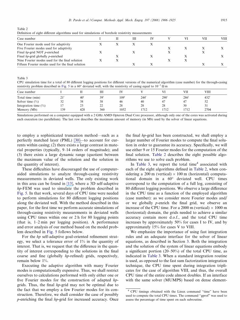
Table 2Definition of eight different algorithms used for simulations of borehole resistivity measurements

Case number I II III IV V VI VII VIII

One Fourier mode used for adaptivity X X X XFive Fourier modes used for adaptivity X X X XFinal hp-grid NOT p-enriched X X X XFinal hp-grid globally p-enriched X X X XNine Fourier modes used for the final solution X X X XFifteen Fourier modes used for the final solution X X X X

Table 3CPU simulation time for a total of 80 different logging positions for different versions of the numerical algorithm (case number) for the through-casingresistivity problem described in Fig. 5 in a 60� deviated well, with the resistivity of casing equal to 10�5 X m

Case number I II III IV V VI VII VIII

Total time (min) 210 400 390 1090 2440 2900 2860 4320

Solver time (%) 32 38 38 46 40 47 47 52Integration time (%) 17 23 22 28 28 28 30 31Memory (Mb) 139 428 360 1052 1712 1712 1712 2704

Simulations performed on a computer equipped with a 2 GHz AMD Opteron Dual Core processor, although only one of the cores was activated duringeach execution (no parallelism). The last row describes the maximum amount of memory (in Mb) used by the solver of linear equations.

4 CPU timings obtained with the Linux command ‘‘time” have beenused to compute the total CPU times. The command ‘‘gprof” was used toassess the percentage of time spent on each subroutine.

D. Pardo et al. / Comput. Methods Appl. Mech. Engrg. 197 (2008) 1906–1925 1915

to employ a sophisticated truncation method—such as aperfectly matched layer (PML) [30]—to account for cur-rents within casing; (2) there exists a large contrast in mate-rial properties (typically, 9–14 orders of magnitude); and(3) there exists a large dynamic range (quotient betweenthe maximum value of the solution and the solution inthe quantity of interest).

These difficulties have discouraged the use of computer-aided simulations to analyze through-casing resistivitymeasurements in deviated wells. The only existing workin this area can be found in [13], where a 3D self-adaptivehp-FEM was used to simulate the problem described inFig. 5. In that work, several days of CPU time were neededto perform simulations for 80 different logging positionsalong the deviated well. With the method described in thispaper, for the first time we perform accurate simulations ofthrough-casing resistivity measurements in deviated wellsusing CPU times within one or 2 h for 80 logging points(that is, 1–2 min per logging position). A performanceand error analysis of our method based on the model prob-lem described in Fig. 5 follows below.

For the hp self-adaptive goal-oriented refinement strat-egy, we select a tolerance error of 1% in the quantity ofinterest. That is, we request that the difference in the quan-tity of interest corresponding to the solutions in the finalcoarse and fine (globally hp-refined) grids, respectively,remain below 1%.

Executing the adaptive algorithm with many Fouriermodes is computationally expensive. Thus, we shall restrictourselves to calculations performed with only either one orfive Fourier modes for the construction of adapted hp-grids. Thus, the final hp-grid may not be optimal due tothe fact that we employ a few Fourier modes for its con-struction. Therefore, we shall consider the case of possiblyp-enriching the final hp-grid for increased accuracy. Once

the final hp-grid has been constructed, we shall employ alarger number of Fourier modes to compute the final solu-tion in order to guarantee its accuracy. Specifically, we willuse either 9 or 15 Fourier modes for the computation of thefinal solution. Table 2 describes the eight possible algo-rithms we use to solve each problem.

In Table 3, we report the total time4 associated witheach of the eight algorithms defined in Table 2, when con-sidering a 200 m (vertical) 100 m (horizontal) computa-tional domain in a 60� deviated well. CPU timescorrespond to the computation of a full log, consisting of80 different logging positions. We observe a large differencein the CPU time as a function of the employed algorithm(case number): as we consider more Fourier modes and/or we globally p-enrich the final grid, we observe anincrease of the CPU time. For a 2000 m (vertical) 1000 m(horizontal) domain, the grids needed to achieve a similaraccuracy contain more d.o.f., and the total CPU timeincreases by approximately 50% for cases I to IV, and byapproximately 15% for cases V to VIII.

We emphasize the importance of using fast integrationrules and an adequate interface for the solver of linearequations, as described in Section 3. Both the integrationand the solution of the system of linear equations embodya significant portion (20–50%) of the total CPU time, asindicated in Table 3. When a standard integration routineis used, as opposed to the fast sum factorization integrationtechnique, the CPU time spent during integration tripli-cates for the case of algorithm VIII, and thus, the overallCPU time of the entire code almost doubles. If an interfacewith the same solver (MUMPS) based on dense element-

1916 D. Pardo et al. / Comput. Methods Appl. Mech. Engrg. 197 (2008) 1906–1925

by-element stiffness matrices is used, then the solver timeincreases by a factor of four or five when considering 15Fourier modes, which severely deteriorates the overall per-formance of the code. The memory used by solverMUMPS also increases significantly as we consider moreFourier modes.

Fig. 6 (top panel) displays the simulated measurementscorresponding to the through-casing resistivity problemdescribed in Fig. 5 in a 60� deviated well, with the resistivityof casing equal to 10�5 X m. Different curves correspond tothe eight algorithms (case numbers) considered in thispaper. We observe that the measured signal is (almost) pro-portional to the formation conductivity. Selecting the solu-tion corresponding to ‘case VIII’ as the reference solution,Fig. 6 (bottom panel) displays the relative error of thequantity of interest corresponding to the remaining seven

10 10 10

0

0.25

0.5

0.75

1

Second difference of potential (V)

Ver

tical

pos

ition

of r

ecei

vers

(m

)V

ertic

al p

ositi

on o

f rec

eive

rs (

m)

Case I

Case II

Case III

Case IV

10 100

102

0

0.25

0.5

0.75

1

Relative error (in %)

Case I

Case II

Case III

Case IV

Fig. 6. Simulated through-casing resistivity measurements in a 60� deviated wDifferent curves correspond to different algorithms summarized in Table 2. TopBottom panel: relative error with respect to the reference solution correspond

cases. For most logging positions, the relative error is con-sistently below 10%. This level of accuracy is enough froman engineering point of view to properly assess the resistiv-ity of the formation. Nonetheless, substantially largererrors (above 100%) are observed in the highly resistivelayer when employing algorithms I and III, which indicatesthe accuracy limitations of those algorithms. Algorithms IIand IV provide a good compromise between accuracy andCPU time.

Fig. 7 displays similar results to those shown in Fig. 6,when considering a larger computational domain, specifi-cally, a domain of size 2000 m (vertical) 1000 m (hori-zontal). These results further illustrate the inaccuratesolutions delivered by algorithms I and III. Again, algo-rithms II and IV provide the best compromise betweenaccuracy and CPU time.

10 10 10

0

0.25

0.5

0.75

1

Second difference of potential (V)

Ver

tical

pos

ition

of r

ecei

vers

(m

)

Case V

Case VI

Case VII

Case VIII

Relative error (in %)10 10

010

2

0

0.25

0.5

0.75

1

Ver

tical

pos

ition

of r

ecei

vers

(m

)

Case V

Case VI

Case VII

ell. Size of computational domain: 200 m (vertical) 100 m (horizontal).panel: solution in the quantity of interest as a function of logging position.

ing to algorithm (case) VIII.

10 10 10

0

0.25

0.5

0.75

1

Second difference of potential (V)

Ver

tical

pos

ition

of r

ecei

vers

(m

)

Case I

Case II

Case III

Case IV

10 10 10

0

0.25

0.5

0.75

1

Second difference of potential (V)

Ver

tical

pos

ition

of r

ecei

vers

(m

)

Case V

Case VI

Case VII

Case VIII

10 10 10

0

0.25

0.5

0.75

1

Second difference of potential (V)

Ver

tical

pos

ition

of r

ecei

vers

(m

)

3D

Case II

Case IV

Case VIII

10 100

102

0

0.25

0.5

0.75

1

Relative error (in %)

Ver

tical

pos

ition

of r

ecei

vers

(m

)CaseV

Case VI

Case VII

Fig. 7. Simulated through-casing resistivity measurements in a 60� deviated well. Size of computational domain: 2000 m (vertical) 1000 m (horizontal).Different curves correspond to different algorithms summarized in Table 2. Top-left, top-right, and bottom-left panels: solution in the quantity of interestas a function of logging position. Bottom-right panel: relative error with respect to the reference solution corresponding to algorithm (case) VIII.

D. Pardo et al. / Comput. Methods Appl. Mech. Engrg. 197 (2008) 1906–1925 1917

From the results shown in Fig. 7 (bottom-left panel), weemphasize the discrepancy between solutions obtained withthis method and the solution obtained with the 3D hp-FEM utilized in [13]. We note that at the points where0.3 m < z < 0.7 m (points of discrepancy between 3D and2D solutions), the 3D hp-FE solution did not converge atthe desired level of accuracy (3%), and the simulationwas stopped after various days of computations. Withthe new method presented in this paper, we have reducedthe computational time from several days to less than 2 h(if we employ, for example, algorithm IV). Also, with thenew method we obtain (almost) identical results as weincrease the number of Fourier modes and/or enrich thefinal hp-grid. This consistency of results among variousgridding algorithms and number of Fourier modes indi-

cates that the discretization errors are small, and therefore,that the solutions obtained with the new method areaccurate.

The above observations confirm that the new method issubstantially more accurate than the 3D hp-FEM. In sum-mary, with the new method we dramatically reduce thecomputational time while we gain accuracy on the finalsolution.

Finally, Fig. 8 analyzes the numerical error due to thetruncation of the computational domain. We comparethe solution obtained with a 200 m (vertical) 100 m (hor-izontal) domain against the solution obtained with a2000 m (vertical) 1000 m (horizontal) domain. A relativedifference below 20% is obtained at all logging points. Fur-thermore, with the exception of a few logging points

10 10 10

0

0.25

0.5

0.75

1

Second difference of potential (V)

Ver

tical

pos

ition

of r

ecei

vers

(m

)

200x100

2000x1000

5 10 15 20

0

0.25

0.5

0.75

1

Relative error (in %)

Ver

tical

pos

ition

of r

ecei

vers

(m

)

200x100 m

Fig. 8. Simulated through-casing resistivity measurements in a 60� deviated well. Different curves correspond to difference sizes of computational domain.Left panel: simulated measurements. Right panel: relative error using the solution on the largest spatial domain (2000 m 1000 m) as the referencesolution.

1918 D. Pardo et al. / Comput. Methods Appl. Mech. Engrg. 197 (2008) 1906–1925

located across the most resistive layer of the formation, thediscrepancy between both solutions remains below 10%.These differences can be neglected from the engineeringpoint of view in the case of through-casing resistivity mea-surements, since the uncertainty of actual field measure-ments is often above the observed level of discrepancy.

Fig. 9. 2D cross-section of an axial-symmetric Laterolog resistivityproblem in a borehole environment. Measurements are based on onecurrent (emitter) and two voltage (collector) electrodes. The subsurfaceearth formation is assumed to be composed of four different horizontallayers with varying resistivities, from 0:5 X m to 20 X m.

4.3.2. Laterolog resistivity measurementsWe now consider Laterolog-type resistivity measure-

ments acquired at zero frequency (DC). This type of mea-surements are widely used by the logging industry when theborehole mud is more electrically conductive than the sur-rounding formation. Fig. 9 describes the correspondinglogging instrument, electrodes, and materials. The current(emitter) electrode is excited by prescribing a constant fluxwith total current equal to 1 A, that is, f ¼ $ � Jimp is equalto one over the volume of the current (emitter) electrode.For the sake of simplicity, we avoid the use of voltagesources (prescribing the electric potential at the source)and bucking electrodes (used to maintain a zero differenceof potential between two electrodes). We note, however,that voltage sources and bucking electrodes may enhancethe dependence of the measurements upon the formationresistivity, and therefore, facilitate a fast inversion of themeasurements. They can be easily modeled using a non-homogeneous Dirichlet BC (for the voltage source) and aslight modification of the resulting system of linear equa-tions as described, for example, in [31] (for modeling buck-ing electrodes).

Table 4 summarizes the CPU time spent by each of theeight algorithms defined in Table 2 for the case of a 60� devi-ated well. CPU times correspond to the computation of afull log, consisting of 80 different logging positions. Eachlogging position is separated by a true vertical distance of

5 cm. In similar fashion to the results summarized in Table3, we observe large differences in the CPU times as a func-tion of the employed algorithm (case number). However,we need only roughly half of the time for simulating Latero-log resistivity measurements compared to that needed tosimulate through-casing resistivity measurements. This

Table 4CPU simulation time for a total of 80 different vertical logging positionsfor different versions of the numerical algorithm (case number) for theLaterolog measurements described in Fig. 9 in a 60� deviated well

Case number I II III IV V VI VII VIII

Total time (min) 110 250 180 830 1260 1530 1580 2790

Simulations performed on a computer equipped with a 2 GHz AMDOpteron Dual Core processor, although only one of the cores was acti-vated during each execution (no parallelism).

D. Pardo et al. / Comput. Methods Appl. Mech. Engrg. 197 (2008) 1906–1925 1919

behavior occurs because fewer unknowns are necessary tosimulate Laterolog resistivity measurements to achieve asimilar level of accuracy.

Fig. 10 (left panel) displays the simulated measure-ments corresponding to the Laterolog resistivity problem

10 10 100

0

0.5

1

1.5

2

2.5

Second difference of potential (V)

Ver

tical

pos

ition

of r

ecei

vers

(m

)

Case ICase IICase IIICase IV

10 100 101 102

0

0.5

1

1.5

2

2.5

Relative error (in %)

Ver

tical

pos

ition

of r

ecei

vers

(m

)

Case ICase IICase IIICase IV

Fig. 10. Simulated Laterolog resistivity measurements acquired in a 60� deviatalgorithm. Left panel: solution in the quantity of interest as a function of losolution corresponding to algorithm (case) VIII.

described in Fig. 9 in a 60� deviated well. Different curvescorrespond to the eight algorithms (case numbers) consid-ered in this paper. We observe a strong correlation betweenthe simulated signal and the formation conductivity.Numerically, we observe that curves obtained using algo-rithms II, IV, V, VI, VII, and VIII are (almost) identical.By selecting the solution corresponding to ‘case VIII’ as ref-erence, Fig. 10 (right panel) displays the relative error of thequantity of interest corresponding to the remaining sevencases. At most logging positions, the relative error remainsbelow 2% for algorithms II, IV, V, VI, and VII. This level ofaccuracy is exceptionally good from the engineering pointof view when assessing the resistivity of the formation.Nonetheless, substantially larger errors (above 60%) areobserved at various logging points when employing algo-

10 10 100

0

0.5

1

1.5

2

2.5

Second difference of potential (V)

Ver

tical

pos

ition

of r

ecei

vers

(m

)

Case VCase VICase VIICase VIII

10 100 101 102

0

0.5

1

1.5

2

2.5

Relative error (in %)

Ver

tical

pos

ition

of r

ecei

vers

(m

)

Case VCase VICase VII

ed well. Different curves correspond to different versions of the simulationgging position. Right panel: Relative error with respect to the reference

1920 D. Pardo et al. / Comput. Methods Appl. Mech. Engrg. 197 (2008) 1906–1925

rithms I and III, as it was also the case with through-casingresistivity measurements. Again, we observe the accuracylimitations associated with these two algorithms: for Late-rolog instruments, algorithms II and IV seem to also pro-vide the best compromise between accuracy and CPU time.

Algorithm IV, which only utilizes one Fourier mode forthe adaptivity, is used to simulate resistivity measurementsin the remainder of this paper.

4.4. Well-logging applications

In this section, we illustrate the applicability of thismethod of solution by studying, for example, the effect ofwater invasion in through-casing resistivity measurementsfor various dip angles. We present the first results, whichare of great interest to the logging industry, and provide aclear physical interpretation of the water invasion effect fordifferent layers in the formation and for various dip angles.

We consider the through-casing resistivity problemdescribed in Fig. 5 and a computational domain of 2000 m(vertical) 1000 m (horizontal). Fig. 11 compares simula-tion results for various dip angles corresponding to casingwith resistivity equal to 10�5 X m (left panel), and 2:310�7 X m (right panel), respectively. We observe that mea-surements simulated in highly deviated wells are propor-tional to the average of the conductivity of formationmaterials surrounding the receivers. As indicated inFig. 11, the minimum and maximum recorded measure-ments increase as we decrease the dip angle. As a functionof the casing resistivity, we observe a dramatic change ofthe intensity of the received signal, as physically expected.However, we observe qualitatively similar results for differ-ent values of casing resistivity. This behavior is consistentwith the result for vertical wells provided by [29], where

10 10 10 10 10

0

0.5

1

1.5

Second difference of potential (V)

Ver

tical

pos

ition

of r

ecei

vers

(m

)

0 degrees

30 degrees

45 degrees

60 degrees

Fig. 11. Simulated through-casing resistivity measurements. Size of computacorrespond to different dip angles: 0�, 30�, 45�, and 60�. Left panel: casin2:3 10�7 X m.

the author indicates that simulation results as a functionof casing resistivity should be qualitatively identical.

In the remainder of this paper, we assume a casing resis-tivity equal to 2:3 10�7 X m, since this is a typical value ofcasing conductivity encountered in actual field applications.

We now consider the effect of water-base mud-filtrateinvasion in the two layers of resistivities equal to0:01 X m (layer 1) and 10; 000 X m (layer 2), respectively.In so doing, we assume a piston-like radial water invasionwith radial length of invasion equal to 10 cm and 50 cm,respectively. For the invaded part of the conductive layer(layer 1), we assume that the layer resistivity after beinginvaded with water is equal to 1 X m. For the invaded partof the resistive layer (layer 2), we assume that the resultingresistivity is equal to 10 X m.

Fig. 12 displays simulation results for the case of invad-ing the conductive layer with water at different dip angles.The effect of water invasion on the simulated measure-ments is qualitatively similar for all dip angles. We observea strong effect on the results due to water injection. Withonly 10 cm of radial length of water invasion, the simulatedmeasurements decrease by approximately one order ofmagnitude. A larger effect ensues when the radius of inva-sion increases to 50 cm. Further increase of the radius ofwater invasion hardly affects the measurements, since theradial length of investigation of these logging instrumentsis relatively short (10–70 cm). We also observe that theeffect of water invasion into layer 1 is non-local, as it affectsmeasurements above and below the layer where water inva-sion takes place.

Fig. 13 displays simulation results for the case of invad-ing the resistive layer with water for different dip angles.We observe that the effect of water invasion on thesimulated measurements is qualitatively similar for all dip

10 10 10 10 10

0

0.5

1

1.5

Second difference of potential (V)

Ver

tical

pos

ition

of r

ecei

vers

(m

)

0 degrees

30 degrees

45 degrees

60 degrees

tional domain: 2000 m (vertical) 1000 m (horizontal). Different curvesg resistivity equal to 10�5 X m. Right panel: casing resistivity equal to

10 10 10 10 10

0

0.5

1

1.5

Second difference of potential (V)

Ver

tical

pos

ition

of r

ecei

vers

(m

)

0 degrees

NO INV

10 cm INV

50 cm INV

10 10 10 10 10

0

0.5

1

1.5

Second difference of potential (V)

Ver

tical

pos

ition

of r

ecei

vers

(m

)

30 degrees

NO INV

10 cm INV

50 cm INV

10 10 10 10 10

0

0.5

1

1.5

Second difference of potential (V)

Ver

tical

pos

ition

of r

ecei

vers

(m

)

45 degrees

NO INV

10 cm INV

50 cm INV

10 10 10 10 10

0

0.5

1

1.5

Second difference of potential (V)

Ver

tical

pos

ition

of r

ecei

vers

(m

)

60 degrees

NO INV

10 cm INV

50 cm INV

Fig. 12. Simulated through-casing resistivity measurements. Casing resistivity equal to 2:3 10�7 X m. Size of computational domain: 2000 m(vertical) 1000 m (horizontal). Different panels correspond to different dip angles: 0 (top-left), 30� (top-right), 45� (bottom-left), and 60� (bottom-right).Different curves correspond to different radial lengths of water invasion into the conductive layer (layer 1): no invasion, 10 cm invasion, and 50 cminvasion.

D. Pardo et al. / Comput. Methods Appl. Mech. Engrg. 197 (2008) 1906–1925 1921

angles. However, in this case we observe that the effect ofwater invasion into layer 2 is local, and that it only affectsthe measurements within the resistive layer. As physicallyexpected, a larger measurement variation ensues when theradius of invasion increases.

5. Discussion about further applications

The method presented in this paper is efficient, reliable,and accurate in various engineering applications, for tworeasons:

� Material properties in the newly defined non-orthogonalsystem of coordinates are constant in the quasi-azi-

muthal direction, and thus, one Fourier mode is suffi-cient to reproduce exactly the material properties (inour case, the conductivity r).� The Jacobian matrix expressing the change of coordi-

nates from Cartesian to the non-orthogonal system ofcoordinates can be represented exactly with only fiveFourier modes.

Thus, the use of this method is limited by the geometri-cal description of the problem. Arbitrary 3D geometrieswill, in general, not satisfy the two properties describedabove. However, the method is physics independent, andcan be applied to simulate diverse measurements in devi-ated wells, such as those based on electrodynamics, sonic

10 10 10 10 10

0

0.5

1

1.5

Second difference of potential (V)

Ver

tical

pos

ition

of r

ecei

vers

(m

)

0 degrees

NO INV

10 cm INV

50 cm INV

10 10 10 10 10

0

0.5

1

1.5

Second difference of potential (V)

Ver

tical

pos

ition

of r

ecei

vers

(m

)

30 degrees

NO INV

10 cm INV

50 cm INV

10 10 10 10 10

0

0.5

1

1.5

Second difference of potential (V)

Ver

tical

pos

ition

of r

ecei

vers

(m

)

45 degrees

NO INV

10 cm INV

50 cm INV

10 10 10 10 10

0

0.5

1

1.5

Second difference of potential (V)

Ver

tical

pos

ition

of r

ecei

vers

(m

)60 degrees

NO INV

10 cm INV

50 cm INV

Fig. 13. Simulated through-casing resistivity measurements. Casing resistivity equal to 2:3 10�7 X m. Size of computational domain: 2000 m(vertical) 1000 m (horizontal). Different panels correspond to different dip angles: 0� (top-left), 30� (top-right), 45� (bottom-left), and 60� (bottom-right).Different curves correspond to different radial lengths of water invasion into the resistive layer (layer 2): no invasion, 10 cm invasion and 50 cm invasion.

1922 D. Pardo et al. / Comput. Methods Appl. Mech. Engrg. 197 (2008) 1906–1925

propagation (acoustics coupled with elasticity), flow inporous media, and geomechanics. An application of thismethod to electrodynamic measurements shall be presentedin a forthcoming paper.

Despite the geometrical limitations inherent to ourmethod, there exists another particular geometry of interestfor logging measurements for which our formulation is alsosuitable: measurements acquired with the logging instru-ment eccentered from the axis of the well. Appendix Bdescribes a suitable change of variables for borehole-eccen-tered measurements. Thus, it is possible to simulate bore-hole-eccentered measurements acquired in deviated wellsby composing the change of coordinates for deviated wellswith the change of coordinates for borehole-eccenteredmeasurements.

The presented method may also be used in combinationwith Perfectly Matched Layers (PML) to truncate the com-

putational domain. Indeed, the interpretation of PML interms of a change of variables in the complex plane(described in [32]), makes the implementation of a PMLtrivial by simply composing the change of variables usedin our method with the change of variables pertaining tothe PML implementation.

In addition, the method described in this paper is idealfor the solution of inverse problems. Since the dip angleof the well is often measured by the logging instrument,and therefore, known a priori, only one Fourier mode isneeded to reproduce exactly the material properties. Inother words, material properties are constant with respectto the quasi-azimuthal variable, whereupon the inverseproblem becomes a 2D problem. Using different grids forthe forward and inverse problems (as proposed in [33]),we realize that only a 2D grid with just one Fourier modeis needed for reproducing the inverse solution (material

D. Pardo et al. / Comput. Methods Appl. Mech. Engrg. 197 (2008) 1906–1925 1923

coefficients). This observation about the dimensionality ofthe inverse problem greatly reduces the computationaleffort needed to solve it. We firmly believe that the methodproposed in this paper will have a great practical impact inthe logging industry, as it allows accurate and inexpensivesimulations of forward and inverse borehole problems.

6. Conclusions

We have introduced and successfully tested a new simu-lation method based on the use of a non-orthogonal systemof coordinates with a Fourier series expansion in one direc-tion. The method is suitable for the simulation of boreholeresistivity logging measurements acquired in deviated wells.For these geometries, material coefficients are constant inthe new system of coordinates, and only five Fourier modesare necessary to reproduce exactly the new materials con-structed by incorporating the change of coordinates. Thenew method is suitable for solving forward and inverseproblems.

The implementation of the new method of solution isbased on the superposition of 2D algorithms. Its imple-mentation requires a fraction of the time needed to developa conventional 3D simulator. In order to achieve efficientcomputer performance, special care was taken during inte-gration, where a sum factorization algorithm is employed.Also, it is essential to use an adequate solver (or solverinterface) that takes advantage of the sparsity of the ensu-ing finite-element matrices.

The new solution method delivers exponential conver-gence rates in terms of the error in the quantity of interestversus the number of Fourier modes. In addition, the band-width of the corresponding system of linear equationsremains bounded (each Fourier mode only interacts withno more than five Fourier modes).

We have validated the method, and illustrated its effi-ciency by solving various forward problems based on bore-hole electrostatic measurements. Results indicate thataccurate solutions are obtained using only a limited num-ber of Fourier modes for the solution (typically, below10), thereby enabling a significant complexity reduction.Specifically, for through-casing borehole resistivity mea-surements, the computational time was dramaticallyreduced from several days (when using a 3D-adaptive hp-FEM code) to less than 2 h (when using the new method).In addition, the consistency and reliability of the resultsindicates that we also gain accuracy.

Acknowledgements

This work was financially supported by The Universityof Texas at Austin’s Joint Industry Research Consortium

on Formation Evaluation sponsored by Anadarko, Aramco,Baker Atlas, British Gas, BHP-Billiton, BP, Chevron,ConocoPhillips, ENI E&P, ExxonMobil, Halliburton,Marathon, Mexican Institute for Petroleum, Hydro, Occi-

dental Petroleum, Petrobras, Schlumberger, Shell E&P,Statoil, TOTAL, and Weatherford International Ltd.

Appendix A. Fourier series expansion of the metric

associated with the non-orthogonal system of coordinates for

deviated wells

All non-zero Fourier modal coefficients

Gk ¼1

2p

Z 2p

0

Gnme�jkf2 df2

of tensor matrix G with respect to variable f2 are given by

G0 ¼1þ 0:5ðh0f 01Þ

2 0 0

0 f21 þ 0:5ðh0f1Þ2 0

0 0 1

0B@

1CA; ðA:1Þ

G1 ¼0 0 0:5h0f 010 0 0:5jh0f1

0:5h0f 01 0:5jh0f1 0

0B@

1CA; ðA:2Þ

G2 ¼0:25ðh0f 01Þ

2 0:25jh20f1f 01 0

0:25jh20f1f 01 �0:25ðh0f1Þ2 0

0 0 0

0B@

1CA; ðA:3Þ

G�1 ¼ G1; and ðA:4ÞG�2 ¼ G2: ðA:5Þ

All non-zero Fourier modal coefficients

ðG�1Þk ¼1

2p

Z 2p

0

Gnme�jkf2 df2

of the inverse tensor matrix G�1 with respect to variable f2

are given by

ðG�1Þ0 ¼

1 0 0

0 1=f21 0

0 0 1þ 0:5h20ððf1=f1Þ2 þ ðf 01Þ

2Þ

0BB@

1CCA; ðA:6Þ

ðG�1Þ1 ¼

0 0 �0:5h0f 01

0 0 �0:5jh0f1=f21

�0:5h0f 01 �0:5jh0f1=f21 0

0BB@

1CCA;

ðA:7Þ

ðG�1Þ2 ¼

0 0 0

0 0 0

0 0 0:25h20ð�ðf1=f1Þ2 þ ðf 01Þ

2Þ

0BB@

1CCA; ðA:8Þ

ðG�1Þ�1 ¼ ðG�1Þ1 and ðA:9Þ

ðG�1Þ�2 ¼ ðG�1Þ2: ðA:10Þ

Remark: We note that G0 6¼ diagð1; f21; 1Þ when h0 6¼ 0.

This fact implies that the axial-symmetric formulation isnot the optimal 2D formulation for approximating results

0 0.5 1

0

0.2

0.4

0.6

0.8

1

x

y

0 0.5 1

0

0.2

0.4

0.6

0.8

1

x

y

Fig. B.1. Left panel: top view of the geometry describing the location of a resistivity tool eccentered in the borehole. The radius of the logging instrumentis equal to q1, and the radius of the borehole is equal to q2, with the distance between the center of the logging instrument and the center of the boreholeequal to q0. Right panel: iso-lines corresponding to the change of coordinates for borehole-eccentered measurements described in Formula B.1, withq0 ¼ 0:3, q1 ¼ 0:5, and q2 ¼ 1.

1924 D. Pardo et al. / Comput. Methods Appl. Mech. Engrg. 197 (2008) 1906–1925

in deviated wells. Furthermore, the optimal 2D formula-tion (in the Fourier sense) for approximating results indeviated wells stems from the approximation G ¼ G0.

Appendix B. Non-orthogonal coordinate system for

borehole-eccentered logging instruments

For borehole-eccentered logging instruments, as the onedescribed in Fig. B.1 (left panel), we introduce the follow-ing non-orthogonal coordinate system f ¼ ðf1; f2; f3Þ interms of the Cartesian coordinate system x ¼ ðx1; x2; x3Þ:

x1 ¼ f1ðf1Þ þ f1 cos f2;

x2 ¼ f1 sin f2;

x3 ¼ f3;

8><>: ðB:1Þ

where f1 is defined by the formula

f1ðf1Þ ¼ f1 ¼q0; f1 < q1;f1�q2

q1�q2q0; q1 6 f1 6 q2;

0; f1 > q2:

8><>: ðB:2Þ

The corresponding derivative is given by

f 01ðf1Þ ¼ f 01 ¼0; f1 < q1;

q0

q1�q2; q1 < f1 < q2;

0; f1 > q2:

8><>: ðB:3Þ

Intuitively, q1 is defined such that f1 < q1 covers the areaoccupied by the eccentered logging instrument, which cor-responds to the interior part of the black circle shown inFig. B.1 (left panel). Outside the borehole, which is identi-fied by the dotted circle shown in Fig. B.1 (left panel), weemploy a cylindrical coordinate system. Finally, the areabetween the logging instrument and the borehole wall is in-tended to ‘‘glue” all subdomains so that the resulting sys-

tem of coordinates is globally continuous, bijective, andwith positive Jacobian.

The Jacobian matrix associated with the above changeof coordinates is given by

J ¼ oxi

ofj

� �i;j¼1;2;3

¼f 01 þ cos f2 �f1 sin f2 0

sin f2 f1 cos f2 0

0 0 1

0B@

1CA:

ðB:4ÞAccordingly, the determinant of the Jacobian jJj is equalto jJj ¼ f1½1þ f 01 cosðf2Þ� > 0 if q0 þ q1 < q2.

For the case of eccentered measurements, the describedchange of coordinates for borehole-eccentered measure-ments has three essential properties that make it suitableand attractive for numerical simulations:

� It is globally continuous, bijective, and with positiveJacobian.� Material properties are constant with respect to the

quasi-azimuthal direction f2.� Only a few Fourier modes in terms of f2 are necessary to

approximate the tensor metric and its inverse.

References

[1] X. Lu, D.L. Alumbaugh, One-dimensional inversion of three-component induction logging in anisotropic media, SEG ExpandedAbstr. 20 (2001) 376–380.

[2] D. Pardo, L. Demkowicz, C. Torres-Verdin, M. Paszynski, Simula-tion of resistivity logging-while-drilling (LWD) measurements using aself-adaptive goal-oriented hp-finite element method, SIAM J. Appl.Math. 66 (2006) 2085–2106.

[3] D. Pardo, C. Torres-Verdin, L. Demkowicz, Simulation of multi-frequency borehole resistivity measurements through metal casingusing a goal-oriented hp-finite element method, IEEE Trans. Geosci.Remote Sens. 44 (2006) 2125–2135.

D. Pardo et al. / Comput. Methods Appl. Mech. Engrg. 197 (2008) 1906–1925 1925

[4] D. Pardo, C. Torres-Verdin, L. Demkowicz, Feasibility study for two-dimensional frequency dependent electromagnetic sensing throughcasing, Geophysics 72 (2007) F111–F118.

[5] L. Tabarovsky, M. Goldman, M. Rabinovich, K. Strack, 2.5Dmodeling in electromagnetic methods of geophysics, J. Appl.Geophys. 35 (1996) 261–284.

[6] J. Zhang, R.L. Mackie, T.R. Madden, 3-D resistivity forwardmodeling and inversion using conjugate gradients, Geophysics 60(1995) 1312–1325.

[7] V.L. Druskin, L.A. Knizhnerman, P. Lee, New spectral Lanczosdecomposition method for induction modeling in arbitrary 3-Dgeometry, Geophysics 64 (3) (1999) 701–706.

[8] G.A. Newman, D.L. Alumbaugh, Three-dimensional inductionlogging problems, part 2: a finite-difference solution, Geophysics 67(2) (2002) 484–491.

[9] S. Davydycheva, V. Druskin, T. Habashy, An efficient finite-difference scheme for electromagnetic logging in 3D anisotropicinhomogeneous media, Geophysics 68 (5) (2003) 1525–1536.

[10] T. Wang, S. Fang, 3-D electromagnetic anisotropy modeling usingfinite differences, Geophysics 66 (5) (2001) 1386–1398.

[11] T. Wang, J. Signorelli, Finite-difference modeling of electromagnetictool response for logging while drilling, Geophysics 69 (1) (2004) 152–160.

[12] D.B. Avdeev, A.V. Kuvshinov, O.V. Pankratov, G.A. Newman, Three-dimensional induction logging problems, part 1: an integral equationsolution and model comparisons, Geophysics 67 (2002) 413–426.

[13] D. Pardo, C. Torres-Verdin, M. Paszynski, Simulation of 3D DCborehole resistivity measurements with a goal-oriented hp finite elementmethod. Part II: through casing resistivity instruments, Comput.Geosci. Preprint available at: www.ices.utexas.edu/%7Epardo, in press.

[14] A. Abubakar, P.M. van den Berg, Nonlinear inversion in electrodelogging in a highly deviated formation with invasion using an obliquecoordinate system, IEEE Trans. Geosci. Remote Sens. 38 (2000) 25–38.

[15] R. Aris, Vectors, Tensors, and the Basic Equations of FluidMechanics, Prentice-Hall, Englewood Cliffs, New Jersey, 1962.

[16] D. Pardo, L. Demkowicz, C. Torres-Verdin, L. Tabarovsky, A goal-oriented hp-adaptive finite element method with electromagneticapplications. Part I: electrostatics, Int. J. Numer. Methods Engrg. 65(2006) 1269–1309.

[17] L. Demkowicz, Computing with hp-Adaptive Finite Elements.Volume I: One and Two Dimensional Elliptic and Maxwell Problems,Chapman and Hall, 2006.

[18] A. Ward, J.B. Pendry, Calculating photonic Green’s functions using anonorthogonal finite-difference time-domain method, Phys. Rev. B 58(1998) 7252–7259.

[19] I. Babuska, B. Guo, Approximation properties of the h–p version ofthe finite element method, Comp. Methods Appl. Mech. Engrg. 133(3–4) (1996) 319–346.

[20] C. Schwab, p- and hp-Finite Element Methods. Theory and Appli-cations in Solid and Fluid Mechanics, in: Numerical Mathematicsand Scientific Computation, The Clarendon Press, Oxford UniversityPress, New York, 1998.

[21] MAPLE: Math Software for Engineers, Educators and Students,www.maplesoft.com, 2007.

[22] P.R. Amestoy, I.S. Duff, J.-Y. L’Excellent, Multifrontal paralleldistributed symmetric and unsymmetric solvers, Comp. MethodsAppl. Mech. Engrg. 184 (2000) 501–520.

[23] P.R. Amestoy, I.S. Duff, J. Koster, J.-Y. L’Excellent, A fullyasynchronous multifrontal solver using distributed dynamic schedul-ing, SIAM J. Matrix Anal. Appl. 23 (1) (2001) 15–41.

[24] P.R. Amestoy, A. Guermouche, J.-Y. L’Excellent, S. Pralet, Hybridscheduling for the parallel solution of linear systems, ParallelComput. 32 (2006) 136–156.

[25] METIS – Family of Multilevel Partitioning Algorithms, www-users.cs.umn.edu/karypis/metis, 2007.

[26] J. Kurtz, Fully automatic hp-adaptivity for acoustic and electromag-netic scattering in three dimensions, Ph.D. Thesis, The University ofTexas at Austin, May 2007.

[27] M. Paszynski, L. Demkowicz, D. Pardo, Verification of goal-orientedhp-adaptivity, Comp. Math. Appl. 50 (2005) 1395–1404.

[28] J.P. Boyd, Chebyshev and Fourier Spectral Methods, second ed.,DOVER Publications Inc., 2000.

[29] A.A. Kaufman, The electrical field in a borehole with casing,Geophysics 55 (1) (1990) 29–38.

[30] D. Pardo, L. Demkowicz, C. Torres-Verdin, C. Michler, PMLenhanced with a self-adaptive goal-oriented hp finite-element methodand applications to through-casing borehole resistivity measurements,SIAM J. Sci. Comput. Preprint available at: www.ices.utexas.edu/%7Epardo, submitted for publication.

[31] B.I. Anderson, Modeling and inversion methods for the interpreta-tion of resistivity logging tool response, Ph.D. thesis, Delft Universityof Technology, 2001.

[32] W.C. Chew, W.H. Weedon, A 3D perfectly matched medium frommodified Maxwell’s equations with stretched coordinates, Microw.Opt. Technol. Lett. 7 (1994) 599–604.

[33] W. Bangerth, A framework for the adaptive finite element solution oflarge inverse problems. I. Basic techniques, Technical Report 2004-39,Institute for Computational Engineering and Sciences, The Universityof Texas at Austin, 2004.