Citation: Liu, L.; Zhang, X.; Ji, Y.;

Wang, X. Acoustic Wave Propagation

in a Borehole with a Gas

Hydrate-Bearing Sediment. J. Mar.

Sci. Eng. 2022, 10, 235. https://

doi.org/10.3390/jmse10020235

Academic Editor: Dimitris

Sakellariou

Received: 13 December 2021

Accepted: 27 January 2022

Published: 10 February 2022

Publisher’s Note: MDPI stays neutral

with regard to jurisdictional claims in

published maps and institutional affil-

iations.

Copyright: © 2022 by the authors.

Licensee MDPI, Basel, Switzerland.

This article is an open access article

distributed under the terms and

conditions of the Creative Commons

Attribution (CC BY) license (https://

creativecommons.org/licenses/by/

4.0/).

Journal of

Marine Science and Engineering

Article

Acoustic Wave Propagation in a Borehole with a GasHydrate-Bearing SedimentLin Liu 1,2,3, Xiumei Zhang 1,2,3,*, Yunjia Ji 1,2,3 and Xiuming Wang 1,2,3

1 State Key Laboratory of Acoustics, Institute of Acoustics, Chinese Academy of Sciences, Beijing 100190, China;liulin@mail.ioa.ac.cn (L.L.); jiyunjia@mail.ioa.ac.cn (Y.J.); wangxm@mail.ioa.ac.cn (X.W.)

2 University of Chinese Academy of Sciences, Beijing 100049, China3 Beijing Engineering Research Center of Sea Deep Drilling and Exploration, Institute of Acoustics,

Chinese Academy of Sciences, Beijing 100190, China* Correspondence: zhangxiumei@mail.ioa.ac.cn

Abstract: A knowledge of wave propagation in boreholes with gas hydrate-bearing sediments,a typical three-phase porous medium, is of great significance for better applications of acousticlogging information on the exploitation of gas hydrate. To study the wave propagation in suchwaveguides based on the Carcione–Leclaire three-phase theory, according to the equations of motionand constitutive relations, a staggered-grid finite-difference time-domain (FDTD) scheme and areal axis integration (RAI) algorithm in a two-dimensional (2D) cylindrical coordinate system areproposed. In the FDTD scheme, the partition method is used to solve the stiff problem, and thenonsplitting perfect matched layer (NPML) scheme is extended to solve the problem of the falsereflection waves from the artificial boundaries of the computational region. In the RAI algorithm,combined with six boundary conditions, the displacement potentials of waves are studied to calculatethe borehole acoustic wavefields. The effectiveness is verified by comparing the results of the twoalgorithms. On this basis, the acoustic logs within a gas hydrate-bearing sediment are investigated.In particular, the wave field in a borehole is analyzed and the amplitude of a Stoneley wave underdifferent hydrate saturations is studied. The results indicate that the attenuation coefficient of theStoneley wave increases with the increase of gas hydrate saturation. The acoustic responses in aborehole embedded in a horizontally stratified hydrate formation are also simulated by using theproposed FDTD scheme. The result shows that the amplitude of the Stoneley wave from the upperinterface is smaller than that from the bottom interface.

Keywords: gas hydrate-bearing sediment; three-phase porous media; borehole acoustic wavefield;staggered-grid finite-difference time-domain; real axis integration; gas hydrate saturation

1. Introduction

Natural gas hydrate is globally widespread in continental margin sediments and per-mafrost regions, it has been recognized as a potential energy source in the 21st century [1,2].The exploration and development technology of natural gas hydrate has been a researchhotspot in recent years [3–7]. Acoustic logging is one of the promising technologies inthe interpretation of formations parameters underground [5,8], where the velocity fromacoustic well logs can be used to distinguish gas hydrate layers along the depth of theborehole. Recent research shows that the attenuation of the first arrival can be used toestimate gas hydrate saturation [9], the precision of the result, however, cannot be guaran-teed [8]. To solve the problem and enrich the applications of borehole acoustic logging datain gas-hydrate production, investigations on wave propagation in the fluid-filled boreholesurrounded by a gas hydrate formation are essential.

In fact, natural gas hydrate-bearing sediments are typical three-phase porous media(solid grain, gas hydrate, and water), which implies a particular topological configuration,

J. Mar. Sci. Eng. 2022, 10, 235. https://doi.org/10.3390/jmse10020235 https://www.mdpi.com/journal/jmse

J. Mar. Sci. Eng. 2022, 10, 235 2 of 26

namely the one where solid grain and gas hydrate form two continuous and interpenetrat-ing solid matrices. Consequently, studies of wave propagation in this complex environmentbecome increasingly important to obtain more detailed reservoir information. Leclaireproposed the percolation theory based on Biot’s theory and analyzed the acoustic wavepropagation in frozen porous media such as frozen soil or permafrost [10]. The theorypredicts three compressional and two shear waves are produced when an acoustic wavepropagates in frozen porous media. However, Leclaire assumed that there was no directcontact between solid grains and ice. On this basis, Carcione et al. put forward a Biot-typethree-phase theory of wave propagation in frozen porous media (three-phase porous media)that allows for the interaction between the solid grain frame and pore solid, which is namedthe Carcione–Leclaire three-phase theory [11]. The Carcione–Leclaire theory predicts threecompressional and two shear waves in a three-phase porous medium: the first kind ofcompressional (P1), shear (S1) waves, the second kind of compressional (P2), shear (S2)waves, and the third kind of compressional (P3) wave. Up to date, much work has beendone to study the characteristics of gas hydrate-bearing sediments [12–18]. However, thereis almost no research on the wave propagation in a borehole surrounded by a hydrateformation, therefore, how to better use the acoustic well logging information to evaluatethe parameters of hydrate formation lacks sufficient theoretical guidance.

RAI and FDTD are two effective methods to simulate the acoustic logs of porous media.Rosenbaum [19] first applied Biot’s theory [20–25] of porous media to the study of acousticlogging in a fluid-saturated porous formation and used the RAI method to simulate thefull waveform of the borehole excited by a monopole source, which is the beginning of thetheoretical study on acoustic logging in porous media. On this basis, several RAI algorithmshave been applied to simulate the acoustic logging in a fluid-saturated porous formation,which is a valid method to deal with the borehole acoustic wavefield of a homogeneousmedium [26–35]. For non-axisymmetric boreholes or inhomogeneous porous media, theRAI has limitations in simulating wave propagating problems. As a complement, the FDTDmethod can deal with the problem of heterogeneity [36]. Guan and Hu [37,38] proposed aparameter averaging technique to deal with the interface of a discontinuous medium andapplied it to the numerical simulation of the wave propagation in fluid-saturated porousmedia. They used the NPML technique [39] to eliminate the false reflected waves from themodel boundaries in numerical simulations of wave propagation. Yan [40] et.al numericallysimulate the acoustic fields excited by a point source in the borehole surrounded by a porousformation using the 3D staggered grid stress–velocity finite difference method. Ou [41]used the FDTD algorithm to simulate the wave propagation in a borehole within a porousmedium and studied the characteristics of the Stoneley wave reflection. These studiesshow that much research has been performed on the acoustic logs with a two-phase porousmedium. However, few attempts have studied the problems related to borehole wavepropagations with a three-phase porous medium.

In this paper, to model the acoustic responses excited by an axisymmetric point sourceon the borehole axis of a gas hydrate-bearing sediment (three-phase porous medium), wepropose both a RAI algorithm and a 2D FDTD scheme. In the RAI algorithm based onthe Carcione–Leclaire three-phase theory [11], we construct the displacement potentials ofthree compressional waves and two shear waves of three phases (solid grain frame, gashydrate, and pore fluid) in the frequency wavenumber domain. In addition, the boundaryconditions of the borehole wall of gas hydrate-bearing sediments are given. On thesebases, combined with the equations of motion and constitutive relations, the boreholeacoustic field of this multiphase porous medium is obtained. In the FDTD scheme, weuse a partition method [11,42,43] to solve the stiff problem. Moreover, to truncate thecomputational region, the NPML scheme is extended to solve the problem of the falsereflection waves from the artificial boundaries of the computational region. In addition,we use the proposed FDTD algorithm to describe the spatial distribution of the acousticfield and the waveforms of the monopole acoustic responses in a gas hydrate-bearingsediment. Further, to explore the influence of gas hydrate saturation on Stoneley wave, we

J. Mar. Sci. Eng. 2022, 10, 235 3 of 26

simulate waveforms in the borehole with different gas hydrate saturations and calculatethe attenuation coefficients. Finally, we simulate the acoustic responses in a horizontallystratified gas hydrate-bearing sediment with the proposed FDTD algorithm. The maincontribution of this paper is to construct and simulate the borehole acoustic fields of naturalgas hydrate-bearing sediments, which expand the knowledge of borehole acoustics inthree-phase media. The research findings can provide a theoretical basis and guidancein applying acoustic logging information for the exploration and evaluation of naturalgas hydrate.

2. Carcione–Leclaire Three-Phase Theory

According to the Carcione–Leclaire three-phase theory [11], combined with the consti-tutive relations and equations of motion, the first-order velocity–stress equations in a gashydrate-bearing sediment can be obtained:

σ(1)ij = (K1θ1 + C12θ2 + C13θ3)δij + 2µ1d(1)ij + µ13d(3)ij , (1)

σ(2) = C12θ1 + K2θ2 + C23θ3, (2)

σ(3)ij = (K3θ3 + C23θ2 + C13θ1)δij + 2µ3d(3)ij + µ13d(1)ij , (3)

where σij is a stress component of the solids; σ represents the stress of the fluid (hereis water); the subscripts and superscripts 1, 2, and 3 denote the solid grains; pore fluidand gas hydrate, respectively; K1, K2, and K3 refer to the bulk moduli; µ1, µ3 and µ13are the shear moduli; C12 denotes the grain–fluid elastic coupling coefficient; C23 is thefluid–hydrate elastic coupling coefficient; C13 represents the grain–hydrate elastic couplingcoefficient; and θm, dij define the strain tensors: θm = ε

(m)ii , d(m)

ij = ε(m)ij − δijθm/3. δ is the

Kronecker symbol.The equations of motion [11] can be expressed as

σ(1)ij,j = ρ11

.v(1)i + ρ12

.v(2)i + ρ13

.v(3)i − b12

(v(2)i − v(1)i

)− b13

(v(3)i − v(1)i

), (4)

σ(2),j = ρ12

.v(1)i + ρ22

.v(2)i + ρ23

.v(3)i + b12

(v(2)i − v(1)i

)+ b23

(v(2)i − v(3)i

), (5)

σ(3)ij,j = ρ13

.v(1)i + ρ23

.v(2)i + ρ33

.v(3)i − b23

(v(2)i − v(3)i

)+ b13

(v(3)i − v(1)i

), (6)

where ρ11, ρ22 and ρ33 represent the mass densities of the effective solid grain, effective fluid,and effective hydrate, respectively; ρ12, ρ13 and ρ23 refer to the coupling mass densities;

b12, b13 and b23 denote the friction coefficients; and.v(m)

i is the temporal derivative of theparticle velocity. Equations (4)–(6) can be rewritten as

.V = γΠ, (7)

where

.V =

(v(1)i , v(2)i , v(3)i

)T,γ =

ρ11 ρ12 ρ13ρ21 ρ22 ρ23ρ31 ρ32 ρ33

−1

, Π =

σ(1)ij,j + b12

(v(2)i − v(1)i

)+ b13

(v(3)i − v(1)i

),

σ(2),i − b12

(v(2)i − v(1)i

)− b23

(v(2)i − v(3)i

),

σ(3)ij,j + b23

(v(2)i − v(3)i

)− b13

(v(3)i − v(1)i

).

In this manner, the following equations of motion are obtained, which are conduciveto the establishing of the numerical simulation method:

.v(1)i = γ11Π1 + γ12Π2 + γ13Π3, (8)

.v(2)i = γ21Π1 + γ22Π2 + γ23Π3, (9)

J. Mar. Sci. Eng. 2022, 10, 235 4 of 26

.v(3)i = γ31Π1 + γ32Π2 + γ33Π3, (10)

where γij and Πi are the elements in the matrices γ and Π. Equations (1)–(3) and (8)–(10)constitute the first-order velocity–stress equations for wave propagation in gas hydratebearing-sediments based on the Carcione–Leclaire theory.

Carcione and Quiroga-Goode discussed the eigenvalues of the propagation matrixof Biot’s acoustic equations in a low-frequency range [42]. Zhao applied the partitionmethod to the staggered high-order finite-difference method [43]. Here, the same methodis employed in our work because of the existence of the friction coefficients b12, b23 andb13 [11,44]. The stiff part can be solved analytically, then the non-stiff part of the velocity–stress equations is treated by the staggered-grid finite-difference method. In this manner,the problem of the small time step caused by the existence of a friction coefficient is avoided.

The stiff part of the velocity–stress differential equations can be written in the matrixform as .

V = AV, (11)

where

A11 = b12(γ12 − γ11) + b13(γ13 − γ11), A12 = b12(γ11 − γ12) + b23(γ13 − γ12),

A13 = b23(γ12 − γ13) + b13(γ11 − γ13), A21 = b12(γ22 − γ12) + b13(γ23 − γ12),

A22 = b23(γ23 − γ22) + b12(γ12 − γ22), A23 = b23(γ22 − γ23) + b13(γ12 − γ23),

A31 = b12(γ23 − γ13) + b13(γ33 − γ13), A32 = b12(γ13 − γ23) + b23(γ33 − γ23),

A33 = b23(γ23 − γ33) + b13(γ13 − γ33).

In the following discussion, the treatment of a porous medium found in Ref. [44]is used for our case. The analytical solution of Equation (11) in a 2D situation can beexpressed as

V(t) = exp(A∆t)V(t− 1), (12)

where

ξ1 = 12

[tr(A)−

√[tr(A)]2 − 4E

], ξ2 = tr(A)− ξ1,

E = A13 A21 − A11 A23 − A13 A31 + A23 A31 + A11 A33 − A21 A33.

exp(A∆t) = I3 − 1−eζ1∆t

ζ1A +

[(1−eζ1∆t)1ζ1(ζ2−ζ1)

− (1−eζ2∆t)ζ1ζ2(ζ2−ζ1)

]A · (A− ζ1I3), · · ·

ξ1 = 12

[tr(A)−

√[tr(A)]2 − 4E

], ξ2 = tr(A)− ξ1,

E = A13 A21 − A11 A23 − A13 A31 + A23 A31 + A11 A33 − A21 A33. ξ1 and ξ2 are twoeigenvalues of exp(S∆t).

A matrix form is used for the non-stiff part of the velocity–stress differential equations, i.e.,

.V = γB, (13)

where B = (σ(1)ij,j , σ

(2),i , σ

(3)ij,j )

T.

3. Finite Difference Scheme3.1. Discretization of Equations in the Carcione–Leclaire Three-Phase Theory

Figure 1 presents a schematic diagram of the acoustic logging model. A fluid-filledborehole is embedded in an unbounded three-phase porous medium (gas hydrate-bearingsediment). With a cylindrical coordinate system (r, z, θ), the borehole axis lies along thecentral axis z of the cylinder, the monopole acoustic source is located at the center of theborehole which is placed at the origin of the coordinate system, the squares representthe receivers. As the medium is axisymmetric, all field quantities are independent of the

J. Mar. Sci. Eng. 2022, 10, 235 5 of 26

θ-coordinate. The borehole radius a is 0.1 m, ρ f denotes the fluid (water) density, and v frepresents the fluid (water) velocity.

Figure 1. Schematic diagram of the acoustic logging model. The fluid-filled borehole is embedded ina three-phase porous medium. The borehole radius a is 0.1 m. The monopole acoustic source andthe receivers are along the borehole axis, and the source is located at the origin of the cylindricalcoordinate system.

First, Equations (1)–(3) in a 2D axisymmetric cylindrical coordinate system can berewritten as

∂

∂t

σ(1)rr

σ(1)θθ

σ(1)zz

σ(1)rz

=

C1

∂∂r +

D1r D1

∂∂z C12

(∂∂r +

1r

)C12

∂∂z E ∂

∂r +Fr F ∂

∂zC1r + D1

∂∂r D1

∂∂z C12

(∂∂r +

1r

)C12

∂∂z

Er + F ∂

∂r F ∂∂z

D1

(∂∂r +

1r

)C1

∂∂z C12

(∂∂r +

1r

)C12

∂∂z F

(∂∂r +

1r

)E ∂

∂z

µ1∂∂z µ1

∂∂r 0 0 1

2 µ13∂∂z

12 µ13

∂∂r

v(1)r

v(1)z

v(2)r

v(2)z

v(3)r

v(3)z

,

(14)

∂σ(2)

∂t = C12(∂v(1)r

∂r + v(1)rr + ∂v(1)z

∂z ) + K2(∂v(2)r

∂r + v(2)rr + ∂v(2)z

∂z )

+C23(∂v(3)r

∂r + v(3)rr + ∂v(3)z

∂z ),(15)

∂

∂t

σ(3)rr

σ(3)θθ

σ(3)zz

σ(3)rz

=

E ∂

∂r +Fr F ∂

∂z C23

(∂∂r +

1r

)C23

∂∂z C2

∂∂r +

D2r D2

∂∂z

Er + F ∂

∂r F ∂∂z C23

(∂∂r +

1r

)C23

∂∂z

C2r + D2

∂∂r D2

∂∂z

F(

∂∂r +

1r

)E ∂

∂z C23

(∂∂r +

1r

)C23

∂∂z D2

(∂∂r +

1r

)C2

∂∂z

12 µ13

∂∂z

12 µ13

∂∂r 0 0 µ3

∂∂z µ3

∂∂r

v(1)r

v(1)z

v(2)r

v(2)z

v(3)r

v(3)z

,

(16)

C1 = K1 +43 µ1, D1 = K1 − 2

3 µ1, C2 = K3 +43 µ3,

D2 = K3 − 23 µ3, E = C13 +

23 µ13, F = C13 − 1

3 µ13,(17)

where σrr, σθθ , σzz and σrz are the components of the bulk stress tensor.

J. Mar. Sci. Eng. 2022, 10, 235 6 of 26

We define the following intermediate vector as the input for the staggered-grid finite-difference algorithm:

W = (v(1)′r , v(1)′z , v(2)′r , v(2)′z , v(3)′r , v(3)′z , σ(1)rr , σ

(1)θθ , σ

(1)zz , σ

(1)rz , σ(2), σ

(3)rr , σ

(3)θθ , σ

(3)zz , σ

(3)rz ). The

non-stiff part in a 2D axisymmetric cylindrical coordinate system can be written as

∂

∂t

v(1)r

v(1)z

v(2)r

v(2)z

v(3)r

v(3)z

=

∂

∂t

v(1)′

r

v(1)′

z

v(2)′

r

v(2)′

z

v(3)′

r

v(3)′

z

+

γ11

(∂∂r +

1r

)− γ11

r 0 γ11∂∂z

0 0 γ11∂∂z γ11

(∂∂r +

1r

)γ21

(∂∂r +

1r

)− γ21

r 0 γ21∂∂z

0 0 γ21∂∂z γ21

(∂∂r +

1r

)γ31

(∂∂r +

1r

)− γ31

r 0 γ31∂∂z

0 0 γ31∂∂z γ31

(∂∂r +

1r

)γ12∂

∂r γ13

(∂∂r +

1r

)− γ13

r 0 γ13∂∂z

γ12∂∂z 0 0 γ13∂

∂z γ13

(∂∂r +

1r

)γ22∂

∂r γ23

(∂∂r +

1r

)− γ23

r 0 γ23∂∂z

γ22∂∂z 0 0 γ23∂

∂z γ23

(∂∂r +

1r

)γ32∂

∂r γ33

(∂∂r +

1r

)− γ33

r 0 γ33∂∂z

γ32∂∂z 0 0 γ33∂

∂z γ33

(∂∂r +

1r

)

σ(1)rr

σ(1)θθ

σ(1)zz

σ(1)rz

σ(2)

σ(3)rr

σ(3)θθ

σ(3)zz

σ(3)rz

,

(18)

where v(1)r and v(1)z , v(2)r and v(2)z , v(3)r and v(3)z refer to the components of the particle-velocity vector of solid grain frame, fluid and gas hydrate, respectively.

To implement a 2D finite-difference algorithm for the solutions of Equations (14)–(16)and (18), all quantities of the stress and velocity components should be discretized instaggered grids. We discretize the velocities and stresses using the staggered-grid finite-difference algorithm. The staggered-grid finite-difference form of the non-stiff part in a2D axisymmetric cylindrical coordinate system can be expressed as (Here we only givethe staggered-grid finite-difference schemes for the solid grain frame including particlevelocity and stress components, which is similar to those of pore fluid and hydrate)

v(1)(n+1/2)r(i+1/2,j) = v(1)r

′ + ∆t[γ11(Drσ(1)(n)rr(i+1/2,j) +

σ(1)(n)rr(i+1/2,j)−σ

(1)(n)θθ(i+1/2,j)

r

+Dzσ(1)(n)rz(i+1/2,j)) + γ12Drσ

(2)(n)(i,j+1/2) + γ13(Drσ

(3)(n)rr(i+1/2,j)

+σ(3)(n)rr(i+1/2,j)−σ

(3)(n)θθ(i+1/2,j)

r + Dzσ(3)(n)rz(i+1/2,j))],

(19)

v(1)(n+1/2)z(i,j+1/2) = v(1)z

′ + ∆t[γ11(Drσ(1)(n)rz(i,j+1/2) +

σ(1)(n)rz(i,j+1/2)

r + Dzσ(1)(n)zz(i,j+1/2))

+γ12Dzσ(2)(n)(i,j+1/2) + γ13(Drσ

(3)(n)rz(i,j+1/2) +

σ(3)(n)rz(i,j+1/2)

r

+Dzσ(3)(n)zz(i,j+1/2))],

(20)

σ(1)(n+1)rr(i,j) = σ

(1)(n)rr(i,j) + ∆t[C1Drv(1)(n+1/2)

r(i,j) + D1v(1)(n+1/2)

r(i,j)r + D1Dzv(1)(n+1/2)

z(i,j)

+C12(Drv(2)(n+1/2)r(i,j) +

v(2)(n+1/2)r(i,j)

r + Dzv(2)(n+1/2)z(i,j) ) + EDrv(3)(n+1/2)

r(i,j)

+Fv(3)(n+1/2)

r(i,j)r + FDzv(3)(n+1/2)

z(i,j) ],

(21)

J. Mar. Sci. Eng. 2022, 10, 235 7 of 26

σ(1)(n+1)θθ(i,j) = σ

(1)(n)θθ(i,j) + ∆t[C1

v(1)(n+1/2)r(i,j)

r + D1Drv(1)(n+1/2)r(i,j) + D1Dzv(1)(n+1/2)

z(i,j)

+C12(Drv(2)(n+1/2)r(i,j) +

v(2)(n+1/2)r(i,j)

r + Dzv(2)(n+1/2)z(i,j) ) + E

v(3)(n+1/2)r(i,j)

r

+FDrv(3)(n+1/2)r(i,j) + FDzv(3)(n+1/2)

z(i,j) ],

(22)

σ(1)(n+1)zz(i,j) = σ

(1)(n)zz(i,j) + ∆t[C1Dzv(1)(n+1/2)

z(i,j) + D1v(1)(n+1/2)

r(i,j)r + D1Drv(1)(n+1/2)

r(i,j)

+C12(Drv(2)(n+1/2)r(i,j) +

v(2)(n+1/2)r(i,j)

r + Dzv(2)(n+1/2)z(i,j) ) + EDzv(3)(n+1/2)

z(i,j)

+Fv(3)(n+1/2)

r(i,j)r + FDrv(3)(n+1/2)

r(i,j) ],

(23)

σ(1)(n+1)rz(i+1/2,j+1/2) = σ

(1)(n)rz(i+1/2,j+1/2) + ∆t[µ1(Dzv(1)(n+1/2)

r(i+1/2,j+1/2) + Drv(1)(n+1/2)z(i+1/2,j+1/2))

+ 12 µ13(Dzv(3)(n+1/2)

r(i+1/2,j+1/2) + Drv(3)(n+1/2)z(i+1/2,j+1/2))],

(24)

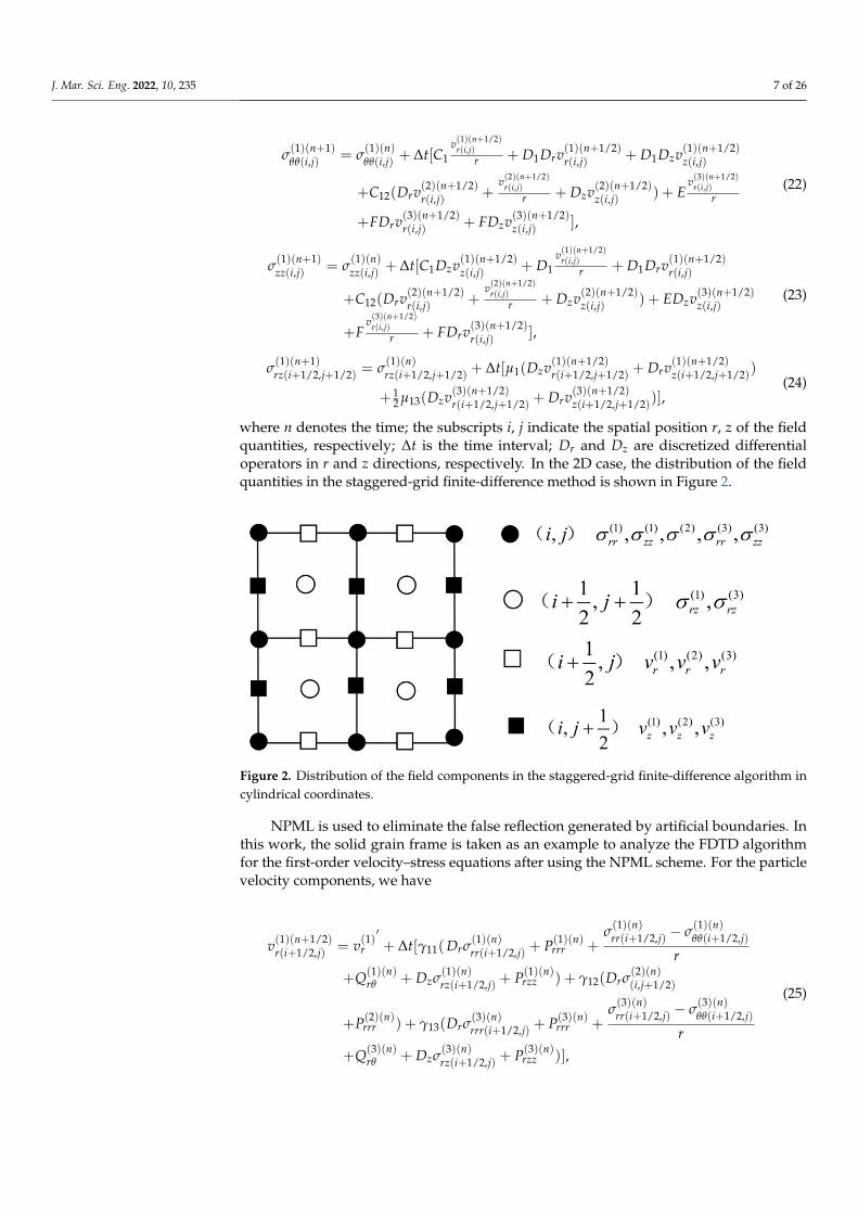
where n denotes the time; the subscripts i, j indicate the spatial position r, z of the fieldquantities, respectively; ∆t is the time interval; Dr and Dz are discretized differentialoperators in r and z directions, respectively. In the 2D case, the distribution of the fieldquantities in the staggered-grid finite-difference method is shown in Figure 2.

Figure 2. Distribution of the field components in the staggered-grid finite-difference algorithm incylindrical coordinates.

NPML is used to eliminate the false reflection generated by artificial boundaries. Inthis work, the solid grain frame is taken as an example to analyze the FDTD algorithmfor the first-order velocity–stress equations after using the NPML scheme. For the particlevelocity components, we have

v(1)(n+1/2)r(i+1/2,j) = v(1)r

′

+ ∆t[γ11(Drσ(1)(n)rr(i+1/2,j) + P(1)(n)

rrr +σ(1)(n)rr(i+1/2,j) − σ

(1)(n)θθ(i+1/2,j)

r+Q(1)(n)

rθ + Dzσ(1)(n)rz(i+1/2,j) + P(1)(n)

rzz ) + γ12(Drσ(2)(n)(i,j+1/2)

+P(2)(n)rrr ) + γ13(Drσ

(3)(n)rrr(i+1/2,j) + P(3)(n)

rrr +σ(3)(n)rr(i+1/2,j) − σ

(3)(n)θθ(i+1/2,j)

r+Q(3)(n)

rθ + Dzσ(3)(n)rz(i+1/2,j) + P(3)(n)

rzz )],

(25)

J. Mar. Sci. Eng. 2022, 10, 235 8 of 26

v(1)(n+1/2)z(i,j+1/2) = v(1)z

′

+ ∆t[γ11(Drσ(1)(n)rz(i,j+1/2) + P(1)(n)

rzr +σ(1)(n)rz(i,j+1/2)

r+Q(1)(n)

rz + Dzσ(1)(n)zz(i,j+1/2) + P(1)(n)

zzz ) + γ12(Dzσ(2)(n)(i,j+1/2)

+P(2)(n)zzz ) + γ13(Drσ

(3)(n)rz(i,j+1/2) + P(3)(n)

rzr +σ(3)(n)rz(i,j+1/2)

r+Q(3)(n)

rz + Dzσ(3)(n)zz(i,j+1/2) + P(3)(n)

zzz )]

(26)

where

Pnrrr = e−Ωr∆tPn−1

rrr −12

Ωr∆t[

e−Ωr∆t ∂σn−1rr∂r

+∂σn

rr∂r

], (27)

Pnzzz = e−Ωz∆tPn−1

zzz −12

Ωz∆t[

e−Ωz∆t ∂σn−1zz∂z

+∂σn

zz∂z

], (28)

Pnrzr = e−Ωr∆tPn−1

rzr −12

Ωr∆t[

e−Ωr∆t ∂σn−1rz∂r

+∂σn

rz∂r

], (29)

Pnrzz = e−Ωz∆tPn−1

rzz −12

Ωz∆t[

e−Ωz∆t ∂σn−1rz∂z

+∂σn

rz∂z

], (30)

Qnrθ = e−Ωr∆tQn−1

rθ − 12

Ωr∆t[e−Ωr∆t

(σn−1

rr − σn−1θθ

)+ σn

rr − σnθθ

], (31)

Qnrz = e−Ωr∆tQn−1

rz − 12

Ωr∆t[e−Ωr∆tσn−1

rz + σnrz

], (32)

Ωp(p) = −Vpml ln α

L

(a

pL+ b

p2

L2

), (33)

Ωr(r) =1r

∫ r

0Ωr(r′)dr′, (34)

where L is the width of the PML, α = 10−6 is a predefined level of wave absorption, andthe coefficients a = 0.25 and b = 0.75 are used.

Similar to the processing of Equations (25) and (26), Equations (21)–(24) can be dis-cretized as

σ(1)(n+1)rr(i,j) = σ

(1)(n)rr(i,j) + ∆t

[C1(Drv(1)(n+1/2)

r(i,j) + P(1)(n+1/2)rr ) + D1(

v(1)(n+1/2)r(i,j)

r+Q(1)(n+1/2)

r ) + D1(Dzv(1)(n+1/2)z(i,j) + P(1)(n+1/2)

zz ) + C12(Drv(2)(n+1/2)r(i,j)

+P(2)(n+1/2)rr +

v(2)(n+1/2)r(i,j)

r+ Q(2)(n+1/2)

r + Dzv(2)(n+1/2)z(i,j) + P(2)(n+1/2)

zz )

+E(Drv(3)(n+1/2)r(i,j) + P(3)(n+1/2)

rr ) + F(v(3)(n+1/2)

r(i,j)

r+ Q(3)(n+1/2)

r )

+F(Dzv(3)(n+1/2)z(i,j) + P(3)(n+1/2)

zz )],

(35)

J. Mar. Sci. Eng. 2022, 10, 235 9 of 26

σ(1)(n+1)θθ(i,j) = σ

(1)(n)θθ(i,j) + ∆t

C1(v(1)(n+1/2)

r(i,j)

r+ Q(1)(n+1/2)

r ) + D1(Drv(1)(n+1/2)r(i,j)

+P(1)(n+1/2)rr ) + D1(Dzv(1)(n+1/2)

z(i,j) + P(1)(n+1/2)zz ) + C12(Drv(2)(n+1/2)

r(i,j)

+P(2)(n+1/2)rr +

v(2)(n+1/2)r(i,j)

r+ Q(2)(n+1/2)

r + Dzv(2)(n+1/2)z(i,j) + P(2)(n+1/2)

zz )

+E(v(3)(n+1/2)

r(i,j)

r+ Q(3)(n+1/2)

r ) + F(Drv(3)(n+1/2)r(i,j) + P(3)(n+1/2)

rr )

+F(Dzv(3)(n+1/2)z(i,j) + P(3)(n+1/2)

zz )],

(36)

σ(1)(n+1)zz(i,j) = σ

(1)(n)zz(i,j) + ∆t[C1(Dzv(1)(n+1/2)

z(i,j) + P(1)(n+1/2)zz

+D1(v(1)(n+1/2)

r(i,j)

r+ Q(1)(n+1/2)

r ) + D1(Drv(1)(n+1/2)r(i,j)

+P(1)(n+1/2)rr ) + C12(Drv(2)(n+1/2)

r(i,j) + P(2)(n+1/2)rr

+v(2)(n+1/2)

r(i,j)

r+ Q(2)(n+1/2)

r + Dzv(2)(n+1/2)z(i,j) + P(2)(n+1/2)

zz )

+E(Dzv(3)(n+1/2)z(i,j) + P(3)(n+1/2)

zz )+F(v(3)(n+1/2)

r(i,j)

r

+Q(3)(n+1/2)r ) + F (Drv(3)(n+1/2)

r(i,j) + P(3)(n+1/2)rr

],

(37)

σ(1)(n+1)rz(i+1/2,j+1/2) = σ

(1)(n)rz(i+1/2,j+1/2) + ∆t[µ1(Dzv(1)(n+1/2)

r(i+1/2,j+1/2) + P(1)(n+1/2)rz

+Drv(1)(n+1/2)z(i+1/2,j+1/2) + P(1)(n+1/2)

zr ) + 12 µ13(Dzv(3)(n+1/2)

r(i+1/2,j+1/2)

+P(3)(n+1/2)rz + Drv(3)(n+1/2)

z(i+1/2,j+1/2) + P(3)(n+1/2)zr )],

(38)

where

Pn+1/2rr = e−Ωr∆tPn−1/2

rr − 12

Ωr∆t

[e−Ωr∆t ∂vn−1/2

r∂r

+∂vn+1/2

r∂r

], (39)

Pn+1/2zz = e−Ωz∆tPn−1/2

zz − 12

Ωz∆t

[e−Ωz∆t ∂vn−1/2

z∂z

+∂vn+1/2

z∂z

], (40)

Pn+1/2zr = e−Ωr∆tPn−1/2

zr − 12

Ωr∆t

[e−Ωr∆t ∂vn−1/2

z∂r

+∂vn+1/2

z∂r

], (41)

Pn+1/2rz = e−Ωz∆tPn−1/2

rz − 12

Ωz∆t

[e−Ωz∆t ∂vn−1/2

r∂z

+∂vn+1/2

r∂z

], (42)

Qn+1/2r = e−Ωr∆tQn−1/2

r − 12

Ωr∆t[e−Ωr∆tvn−1/2

z + vn+1/2z

], (43)

3.2. Discretization of the Equations in the Borehole and Borehole Wall

To unify the equations of acoustic wave propagation in both the outer three-phaseporous medium and the inner fluid in the borehole, the limits of certain field quantitiesand medium parameters in the three-phase porous medium are set to obtain the equationsfor the fluid. In this limiting case, the stresses of the solid grain frame phase and the gas

J. Mar. Sci. Eng. 2022, 10, 235 10 of 26

hydrate phase in the first-order velocity–stress equations of the three-phase porous mediumare zero. The parameters in the Carcione–Leclaire three-phase theory change to

φ = 1,K1 = K3 = 0,K2 = K f ,C12 = C23 = C13 = 0,µ1 = µ13 = µ3 = 0,ρ11 = ρ12 = ρ13 = ρ33 = ρ23 = 0,ρ22 = ρ f .

(44)

In addition, according to the wave equations in fluid, it can be directly defined

exp(A11∆t) = exp(A12∆t) = exp(A13∆t)= exp(A21∆t) = exp(A22∆t) = exp(A23∆t)= exp(A31∆t) = exp(A32∆t) = exp(A33∆t) = 0,γ11 = γ13 = γ21 = γ23 = γ31 = γ33 = 0,γ12 = γ22 = γ32 = 1

ρ f.

(45)

Therefore, the equations of a three-phase porous medium degenerate into governingequations in the fluid.

4. RAI Algorithm

In the frequency wavenumber domain, the acoustic field in the borehole can beexpressed as

ϕ(r, k, ω) =iF

ρ f ω2

[K0

(α f r)+A(k, ω)I0

(α f r)]

, (46)

where F denotes the frequency of the source; A is an undetermined coefficient, which canbe regarded as the reflection coefficient of the wellbore; K0 and I0 are Bessel functions; rrefers to the radial wave number of the fluid.

The acoustic field in a three-phase porous medium can be expressed by the displace-ments of solid grain frame u1, pore fluid u2 and gas hydrate u3. The three displacementsproduced by a point source can be written as

u1 = ∇ϕ1 +∇×∇× (η1z),u2 = ∇ϕ2 +∇×∇× (η2z),u3 = ∇ϕ3 +∇×∇× (η3z),

(47)

where ϕm and ηm represent the displacements of compressional waves (P1, P2 and P3) andshear waves (S1 and S2), respectively. The subscripts m = 1, 2, 3 refer to the solid grain frame,pore fluid and hydrate, respectively. The displacement potentials of the compressionalwaves in the frequency wave number domain can be expressed as

ϕ1(r, k, ω) = iF2ρ f ω2 [B1K0(αP1r) + C1K0(αP2r) + D1K0(αP3r)],

ϕ2(r, k, ω) = iF2ρ f ω2 [B2K0(αP1r) + C2K0(αP2r) + D2K0(αP3r)],

ϕ3(r, k, ω) = iF2ρ f ω2 [B3K0(αP1r) + C3K0(αP2r) + D3K0(αP3r)],

(48)

where Bm, Cm and Dm are the undetermined amplitudes of the three compressional waves,respectively; αP1, αP2 and αP3 are the radial wave numbers of the three compressional

J. Mar. Sci. Eng. 2022, 10, 235 11 of 26

waves, respectively. Moreover, in the frequency wavenumber domain, the displacementpotentials of shear waves are given as

η1(r, k, ω) = iF2ρ f ω2 [E1K0(αS1r) + F1K0(αS2r)],

η2(r, k, ω) = iF2ρ f ω2 [E2K0(αS1r) + F2K0(αS2r)],

η3(r, k, ω) = iF2ρ f ω2 [E3K0(αS1r) + F3K0(αS2r)],

(49)

where Em and Fm are the undetermined amplitudes of the two shear waves, respectively;αS1 and αS2 are the radial wave numbers of the two shear waves, respectively.

In the above formulas, A, Bm, Cm, Dm, Em and Fm are undetermined coefficients, whichare determined by the boundary conditions of the borehole wall. Assuming that there is arelationship between the compressional wave displacement of each phase:

ϕ2 = l1 ϕ1 = l2 ϕ3, (50)

then we can obtainB2 = l11B1, C2 = l12C1, D2 = l13D1,B3 = l11

l21B1, C3 = l12

l22C1, D3 = l13

l23D1.

(51)

Assuming that there is a relationship between the shear wave displacement of each phase:

η2 = l3η1 = l4η3, (52)

then we can getE2 = l31E1, F2 = l32F1,E3 = l31

l41E1, F3 = l32

l42F1.

(53)

The boundary conditions studied in this paper are the open hole boundary conditions,which can be written as

urin = ursout + urhout + w,−φsPf in = σrrsout,−φhPf in = σrrhout,Pf in = Pf out,τrzsout = 0,τrzhout = 0,

(54)

where the subscripts in and out refer to inside and outside the borehole wall, respectively,and the subscripts s, f, and h denote solid grains, pore fluid, and hydrate, respectively. Thefirst equation represents the continuity of fluid flow in the normal direction of the boreholewall. The second and the third equations show that the pressure of fluid in the well in thenormal direction of the borehole wall is equal to the normal stress of the unit body in thegas hydrate formation outside the well in the normal direction of the borehole wall. Thefourth equation represents that the pressure of the fluid in the well in the normal directionof the interface should be equal to that of the unit body in the porous formation outsidethe well. The fifth and sixth equations represent the continuity of shear stresses in thetangential direction of the borehole wall. wp and ws are the flowing displacement of thecompressional and shear wave, which can be expressed as

wP = φ f (u2 − (1− I)u1 − Iu3) = φ f (l1 − (1− I)− Il1l2)u1, (55)

wS = φ f (u2 − (1− I)u1 − Iu3) = φ f (l3 − (1− I)− Il3l4)u1, (56)

where φs, φ f and φh refer to the volume fraction of solid grains, pore fluid, and gas hydrate,respectively. I = φh

φh+φs, φs + φ f + φh = 1, φ f + φh = φ. The number of boundary conditions

is equal to the number of undetermined coefficients in the medium inside and outside the

J. Mar. Sci. Eng. 2022, 10, 235 12 of 26

well. The following linear equations can be obtained by combining the displacement of thecompressional and shear wave potentials and the boundary conditions of each phase

m11 m12 m13 m14 m15 m16m21 m22 m23 m24 m25 m26m31 m32 m33 m34 m35 m36m41 m42 m43 m44 m45 m46m51 m52 m53 m54 m55 m56m61 m62 m63 m64 m65 m66

A1B1C1D1E1F1

=

b1b2b3b400

. (57)

The specific solving process of each parameter in matrix M is shown in Appendix A.The reflection coefficient A in the borehole is given by

A =

b1 m12 m13 m14 m15 m16b2 m22 m23 m24 m25 m26b31 m32 m33 m34 m35 m36b4 m42 m43 m44 m45 m460 m52 m53 m54 m55 m560 m62 m63 m64 m65 m66

|M| . (58)

By substituting Equation (58) into Equation (46), the actual waveform received in thetime domain can be obtained by the double Fourier transform.

5. Numerical Modeling5.1. Homogeneous Three-Phase Porous Media

Figure 3 gives the simulated waveforms of the FDTD and the RAI method at differentlocations from z = 0.5 m to z = 4 m with different source dominant frequencies 6 kHz and10 kHz in the gas hydrate formation. The physical parameters of the gas hydrate-bearingsediment are given in Table 1. The acoustic source pulse width Tc = 0.5 ms is employed inour simulation. The radius of the borehole is 0.1 m. In our FDTD scheme, the time step is2× 10−4 ms and the space steps in the r and z directions are both chosen as 5× 10−4 m.The radial length of the model is 0.5 m, while the axial length is 4.0 m. The width L of theNPML region is 0.5 m. The source pulse function s(t) used in this paper is expressed as

s(t) =

12

[1 + cos 2π

Tc

(t− Tc

2

)]cos 2π f0

(t− Tc

2

), 0 ≤ t ≤ Tc

0 , t > Tc, (59)

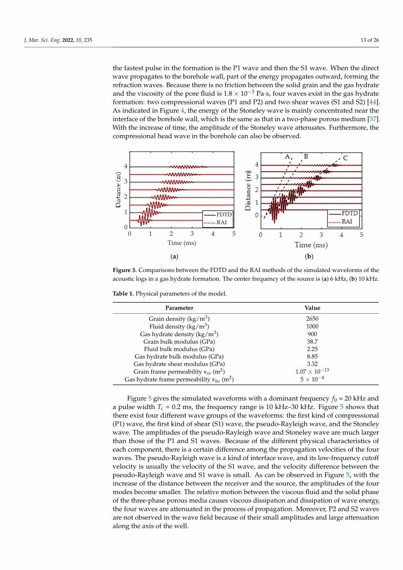
where f0 refers to the center frequency of the source, and t denotes the time. Figure 3bshows that there are three different wave groups of the waveforms: the first kind ofcompressional (P1) wave (A), the first kind of shear (S1) wave (B), and the Stoneley wave(C). The amplitude of the P1 wave is small, while the S1 wave and Stoneley wave are moreevident. As depicted in Figure 3, the FDTD algorithm simulations (black solid lines) agreewell with the RAI solutions (red dash-dot lines) at different locations from z = 0.5 m toz = 4 m. Because of the discrete Fourier transform of the RAI method and the discreteFDTD grids, there are small differences in the amplitudes of the waveforms of the twomethods [41].

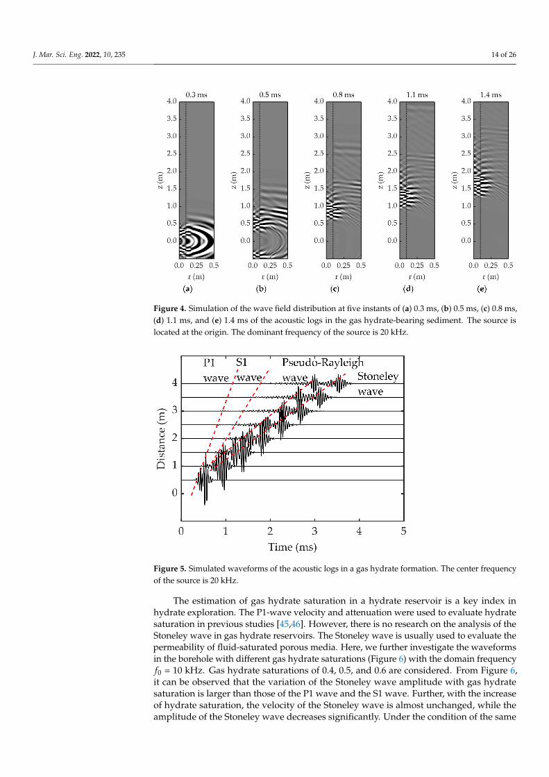
As an example of using the finite-difference scheme proposed above, we simulatethe acoustic field in a wellbore surrounded by a three-phase porous medium. The wavefield distribution at instants of 0.3, 0.5, 0.8, 1.1, and 1.4 ms is displayed in Figure 4. Theblack dotted line represents the borehole wall. To identify different wave groups in thewave field, a domain frequency f0= 20 kHz and a shorter pulse width Tc = 0.2 ms areemployed in our simulation. The time and space steps are consistent with those in Figure 3.Figure 4a–e shows that there is no evident wave reflection from the outer boundaries, whichindicates that the wave field is well absorbed in the NPML. In Figure 4a, we can observe

J. Mar. Sci. Eng. 2022, 10, 235 13 of 26

the fastest pulse in the formation is the P1 wave and then the S1 wave. When the directwave propagates to the borehole wall, part of the energy propagates outward, forming therefraction waves. Because there is no friction between the solid grain and the gas hydrateand the viscosity of the pore fluid is 1.8× 10−3 Pa·s, four waves exist in the gas hydrateformation: two compressional waves (P1 and P2) and two shear waves (S1 and S2) [44].As indicated in Figure 4, the energy of the Stoneley wave is mainly concentrated near theinterface of the borehole wall, which is the same as that in a two-phase porous medium [37].With the increase of time, the amplitude of the Stoneley wave attenuates. Furthermore, thecompressional head wave in the borehole can also be observed.

J. Mar. Sci. Eng. 2022, 10, x. https://doi.org/10.3390/xxxxx www.mdpi.com/journal/jmse

(a) (b)

Figure 3. Comparisons between the FDTD and the RAI methods of the simulated waveforms of the

acoustic logs in a gas hydrate formation. The center frequency of the source is (a) 6 kHz, (b) 10 kHz.

0 1 2 3 4 5

Time (ms)

0

1

2

3

4

FDTD

RAI

Figure 3. Comparisons between the FDTD and the RAI methods of the simulated waveforms of theacoustic logs in a gas hydrate formation. The center frequency of the source is (a) 6 kHz, (b) 10 kHz.

Table 1. Physical parameters of the model.

Parameter Value

Grain density (kg/m3) 2650Fluid density (kg/m3) 1000

Gas hydrate density (kg/m3) 900Grain bulk modulus (GPa) 38.7Fluid bulk modulus (GPa) 2.25

Gas hydrate bulk modulus (GPa) 8.85Gas hydrate shear modulus (GPa) 3.32Grain frame permeability κso (m2) 1.07 × 10−13

Gas hydrate frame permeability κho (m2) 5 × 10−4

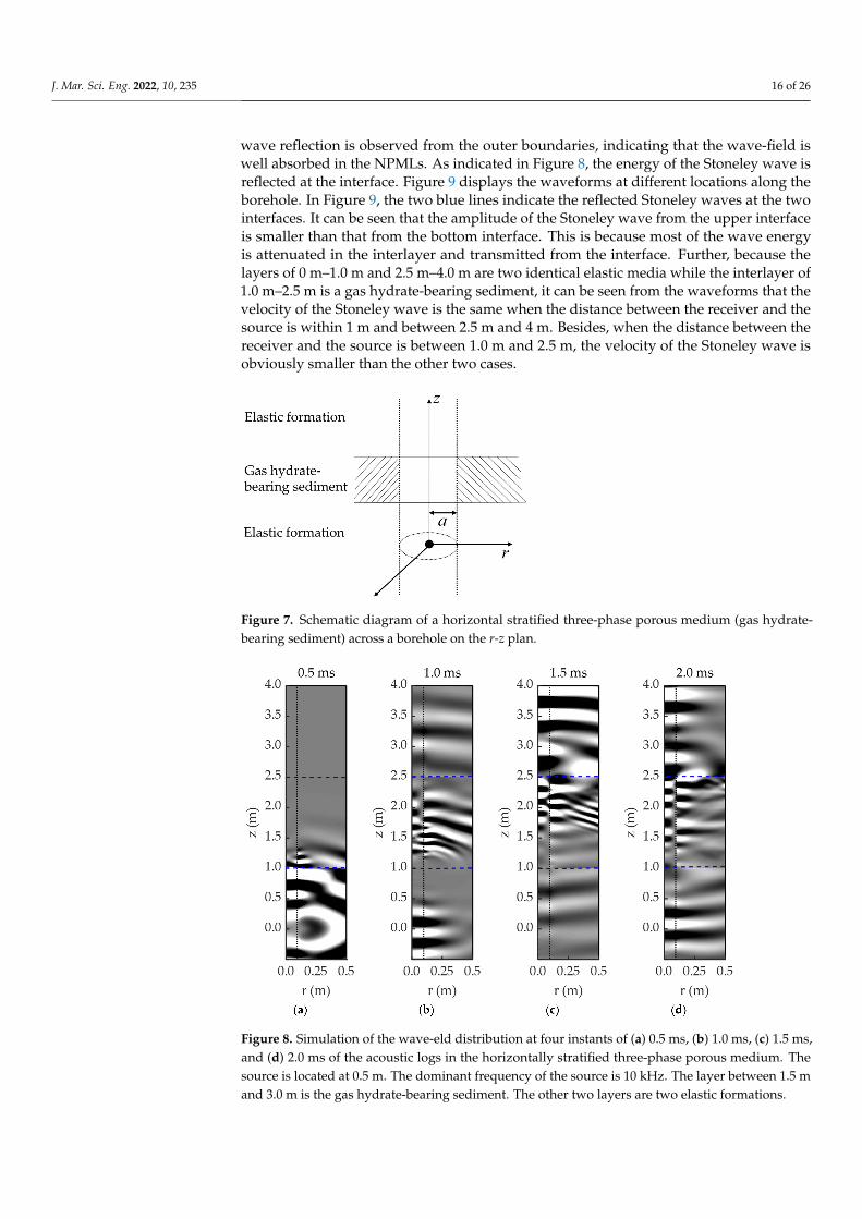
Figure 5 gives the simulated waveforms with a dominant frequency f0 = 20 kHz anda pulse width Tc = 0.2 ms, the frequency range is 10 kHz–30 kHz. Figure 5 shows thatthere exist four different wave groups of the waveforms: the first kind of compressional(P1) wave, the first kind of shear (S1) wave, the pseudo-Rayleigh wave, and the Stoneleywave. The amplitudes of the pseudo-Rayleigh wave and Stoneley wave are much largerthan those of the P1 and S1 waves. Because of the different physical characteristics ofeach component, there is a certain difference among the propagation velocities of the fourwaves. The pseudo-Rayleigh wave is a kind of interface wave, and its low-frequency cutoffvelocity is usually the velocity of the S1 wave, and the velocity difference between thepseudo-Rayleigh wave and S1 wave is small. As can be observed in Figure 5, with theincrease of the distance between the receiver and the source, the amplitudes of the fourmodes become smaller. The relative motion between the viscous fluid and the solid phaseof the three-phase porous media causes viscous dissipation and dissipation of wave energy,the four waves are attenuated in the process of propagation. Moreover, P2 and S2 wavesare not observed in the wave field because of their small amplitudes and large attenuationalong the axis of the well.

J. Mar. Sci. Eng. 2022, 10, 235 14 of 26

Figure 4. Simulation of the wave field distribution at five instants of (a) 0.3 ms, (b) 0.5 ms, (c) 0.8 ms,(d) 1.1 ms, and (e) 1.4 ms of the acoustic logs in the gas hydrate-bearing sediment. The source islocated at the origin. The dominant frequency of the source is 20 kHz.

Figure 5. Simulated waveforms of the acoustic logs in a gas hydrate formation. The center frequencyof the source is 20 kHz.

The estimation of gas hydrate saturation in a hydrate reservoir is a key index inhydrate exploration. The P1-wave velocity and attenuation were used to evaluate hydratesaturation in previous studies [45,46]. However, there is no research on the analysis of theStoneley wave in gas hydrate reservoirs. The Stoneley wave is usually used to evaluate thepermeability of fluid-saturated porous media. Here, we further investigate the waveformsin the borehole with different gas hydrate saturations (Figure 6) with the domain frequencyf0 = 10 kHz. Gas hydrate saturations of 0.4, 0.5, and 0.6 are considered. From Figure 6,it can be observed that the variation of the Stoneley wave amplitude with gas hydratesaturation is larger than those of the P1 wave and the S1 wave. Further, with the increaseof hydrate saturation, the velocity of the Stoneley wave is almost unchanged, while theamplitude of the Stoneley wave decreases significantly. Under the condition of the same

J. Mar. Sci. Eng. 2022, 10, 235 15 of 26

gas hydrate saturation, with the increase of the source-receiver distance, the Stoneley waveattenuates, and its amplitude decreases. Further, the attenuation coefficient of the Stoneleywave is calculated at different gas hydrate saturations. The amplitude of Stoneley waveA [47] can be expressed as

A =

M∑

i=1(Wi)

2

M

12

, (60)

where M is sampling numbers; Wi denotes the amplitude of the sampling point i. Theattenuation coefficient of the Stoneley wave [47] is given by

αST =2lg(An/Am)

(m− n)ds, (61)

where An and Am represent the amplitudes of the received waveforms of the n-th and them-th receivers, respectively; ds is the receiver spacing. After calculation, we find that whenvalues of the hydrate saturation are 0.4, 0.5, and 0.6, the attenuation coefficients of theStoneley wave are 0.35, 0.52, and 0.87, respectively. The results indicate that the attenuationcoefficient of the Stoneley wave increases with the increase of gas hydrate saturation. Thus,we can use the attenuation of the Stoneley wave to estimate the gas hydrate saturation ofthe reservoir.

Figure 6. Simulated waveforms of the acoustic logs in a gas hydrate formation of different gashydrate saturations. Gas hydrate saturation of 0.4, 0.5, and 0.6 are considered. The center frequencyof the source is 10 kHz.

5.2. Horizontally Stratified Three-Phase Porous Medium

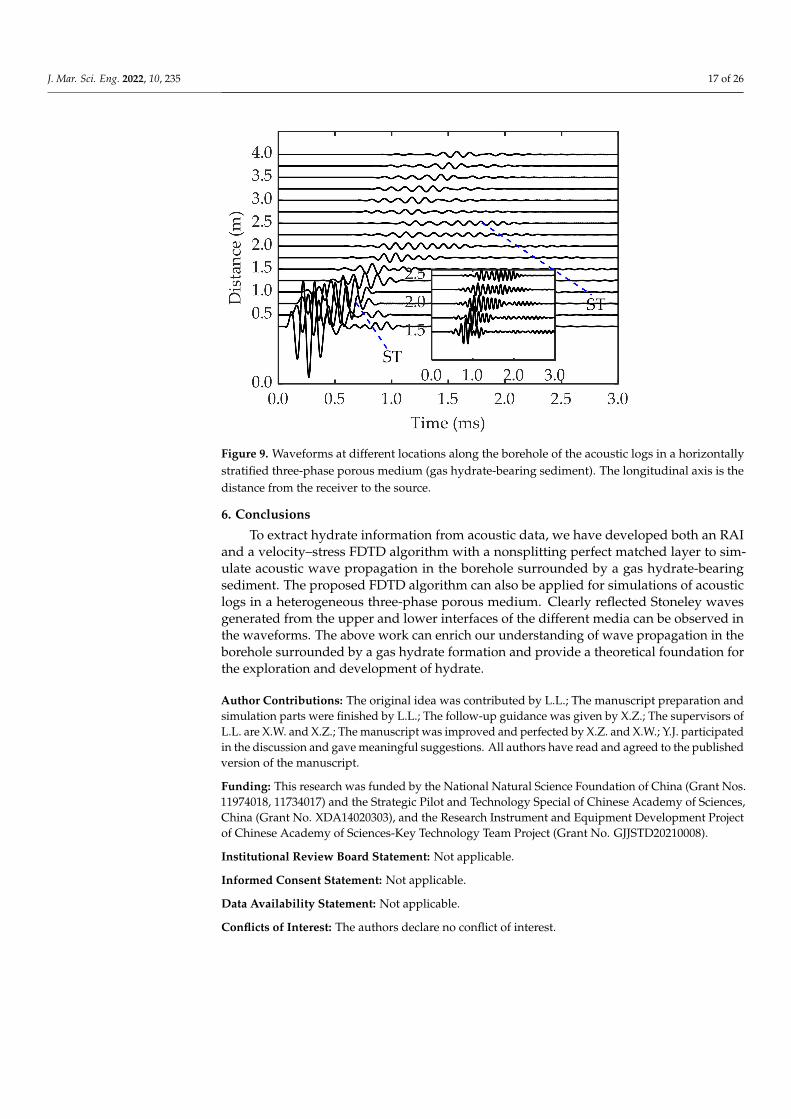
Presented in Figure 7 is a schematic diagram of a horizontally stratified medium acrossa borehole on the r–z plan. The borehole is filled with water. As shown in Figure 7, thereare three layers in the formation around the borehole, the layer between 1.0 m and 2.5 m isthe gas hydrate-bearing sediment, the other two layers are elastic media. The parameters ofthe gas hydrate formation are consistent with those shown in Table 1, while the parametersin the other two elastic layers are the same as those of the solid grains in the hydrateformation. Fluid–hydrate, solid–hydrate, and fluid–solid interfaces exist in this model. Weuse the FDTD algorithm combined with the parameter averaging technique to simulatethe wave propagation in the borehole. Shown in Figure 8 is the wave-field distributionat instants of 0.5, 1.0, 1.5, and 2.0 ms. The interfaces are marked with two blue lines. Inour simulation, the source has a center frequency and a pulse width of f0 = 10 kHz and apulse width Tc = 0.5 ms, the frequency range is 6 kHz–14 kHz. The time and space steps areconsistent with those in the homogeneous three-phase medium. In the figure, no evident

J. Mar. Sci. Eng. 2022, 10, 235 16 of 26

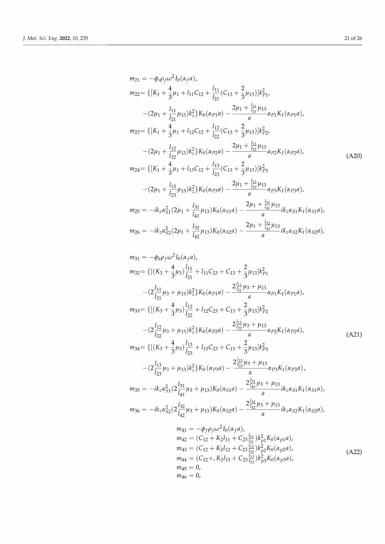
wave reflection is observed from the outer boundaries, indicating that the wave-field iswell absorbed in the NPMLs. As indicated in Figure 8, the energy of the Stoneley wave isreflected at the interface. Figure 9 displays the waveforms at different locations along theborehole. In Figure 9, the two blue lines indicate the reflected Stoneley waves at the twointerfaces. It can be seen that the amplitude of the Stoneley wave from the upper interfaceis smaller than that from the bottom interface. This is because most of the wave energyis attenuated in the interlayer and transmitted from the interface. Further, because thelayers of 0 m–1.0 m and 2.5 m–4.0 m are two identical elastic media while the interlayer of1.0 m–2.5 m is a gas hydrate-bearing sediment, it can be seen from the waveforms that thevelocity of the Stoneley wave is the same when the distance between the receiver and thesource is within 1 m and between 2.5 m and 4 m. Besides, when the distance between thereceiver and the source is between 1.0 m and 2.5 m, the velocity of the Stoneley wave isobviously smaller than the other two cases.

Figure 7. Schematic diagram of a horizontal stratified three-phase porous medium (gas hydrate-bearing sediment) across a borehole on the r-z plan.

Figure 8. Simulation of the wave-eld distribution at four instants of (a) 0.5 ms, (b) 1.0 ms, (c) 1.5 ms,and (d) 2.0 ms of the acoustic logs in the horizontally stratified three-phase porous medium. Thesource is located at 0.5 m. The dominant frequency of the source is 10 kHz. The layer between 1.5 mand 3.0 m is the gas hydrate-bearing sediment. The other two layers are two elastic formations.

J. Mar. Sci. Eng. 2022, 10, 235 17 of 26

Figure 9. Waveforms at different locations along the borehole of the acoustic logs in a horizontallystratified three-phase porous medium (gas hydrate-bearing sediment). The longitudinal axis is thedistance from the receiver to the source.

6. Conclusions

To extract hydrate information from acoustic data, we have developed both an RAIand a velocity–stress FDTD algorithm with a nonsplitting perfect matched layer to sim-ulate acoustic wave propagation in the borehole surrounded by a gas hydrate-bearingsediment. The proposed FDTD algorithm can also be applied for simulations of acousticlogs in a heterogeneous three-phase porous medium. Clearly reflected Stoneley wavesgenerated from the upper and lower interfaces of the different media can be observed inthe waveforms. The above work can enrich our understanding of wave propagation in theborehole surrounded by a gas hydrate formation and provide a theoretical foundation forthe exploration and development of hydrate.

Author Contributions: The original idea was contributed by L.L.; The manuscript preparation andsimulation parts were finished by L.L.; The follow-up guidance was given by X.Z.; The supervisors ofL.L. are X.W. and X.Z.; The manuscript was improved and perfected by X.Z. and X.W.; Y.J. participatedin the discussion and gave meaningful suggestions. All authors have read and agreed to the publishedversion of the manuscript.

Funding: This research was funded by the National Natural Science Foundation of China (Grant Nos.11974018, 11734017) and the Strategic Pilot and Technology Special of Chinese Academy of Sciences,China (Grant No. XDA14020303), and the Research Instrument and Equipment Development Projectof Chinese Academy of Sciences-Key Technology Team Project (Grant No. GJJSTD20210008).

Institutional Review Board Statement: Not applicable.

Informed Consent Statement: Not applicable.

Data Availability Statement: Not applicable.

Conflicts of Interest: The authors declare no conflict of interest.

J. Mar. Sci. Eng. 2022, 10, 235 18 of 26

List of Symbols:b12 friction coefficient between the solid grain frame and pore fluidb13 friction coefficient between the solid grain frame and gas hydrateb23 friction coefficient between the pore fluid and gas hydrateφs volume fraction of solid grainφ f volume fraction of pore fluidφh volume fraction of gas hydrateρs solid grain densityρ f fluid densityρh gas hydrate densityκs0 permeability of solid-grain frameκh0 permeability of gas–hydrate frameKs solid grain bulk modulusK f fluid bulk modulusKh gas hydrate bulk modulusµs solid grain shear modulusµh gas hydrate shear modulusρ11 ρ11 = φsρsa13 + (a21 − 1)φ f ρ f + (a31 − 1)φhρhρ12 ρ12 = −(a21 − 1)φ f ρ f ,ρ22 ρ22 = (a21 + a23 − 1)φ f ρ fρ23 ρ23 = −(a23 − 1)φ f ρ fρ33 ρ33 = φhρha31 + (a23 − 1)φ f ρ f + (a13 − 1)φsρs

a21tortuosity for fluid flowing through the solid grain framea21 = 1 + r12φs(φ f ρ f + φhρh)/φ f ρ f (φw + φh)

a23tortuosity for fluid flowing through the gas hydratea23 = 1 + r23φh(φ f ρ f + φsρs)/φ f ρ f (φ f + φs)

a13tortuosity for solid grain flowing through the gas hydratea13 = 1 + r13φh(φsρs + φhρh)/φsρs(φs + φh)

a31tortuosity for gas hydrate flowing through the solid graina31 = 1 + r31φs(φsρs + φhρh)/φhρh(φs + φh)

K1 K1 = [(1− c1)φs]2Kav + Ksm

K2 φ2f Kav

K3 K3 = [(1− c3)φh]2Kav + Khm

Kavaverage bulk modulus

Kav =[(1− c1)φs/Ks + φ f /K f + (1− c3)φh/Kh

]−1

µ1 µ1 = [(1− g1)φs]2µav + µsm

µ3 µ3 = [(1− g3)φh]2µav + µhm

µ13 µ13 = (1− g1)(1− g3)µav

µavaverage shear modulus

µav =[(1− g1)φs/µs + φ f /iωη f + (1− c3)φh/µh

]−1

c1 and g1consolidation coefficient for the solidc1 = Ksm/φsKs, g1 = µsm/φsµs

c3 and g3consolidation coefficient for the solidc3 = Khm/φhKh, g3 = µhm/φhµh

Appendix A

Equations (50)–(53) show the relationship between the unknown coefficients in dis-placements of compressional and shear waves of each phase. Therefore, in the frequencywavenumber domain, the displacement potential of compressional and shear waves can beexpressed as

ϕ1(r, k, ω) = iF2ρ f ω2 [B1K0(αP1r) + C1K0(αP2r) + D1K0(αP3r)],

ϕ2(r, k, ω) = iF2ρ f ω2 [l11B1K0(αP1r) + l12C1K0(αP2r) + l13D1K0(αP3r)],

ϕ3(r, k, ω) = iF2ρ f ω2 [

l11l21

B1K0(αP1r) + l12l22

C1K0(αP2r) + l13l23

D1K0(αP3r)],

(A1)

J. Mar. Sci. Eng. 2022, 10, 235 19 of 26

η1(r, k, ω) = iF2ρ f ω2 [E1K0(αS1r) + F1K0(αS2r)],

η2(r, k, ω) = iF2ρ f ω2 [l31E1K0(αS1r) + l32F1K0(αS2r)],

η3(r, k, ω) = iF2ρ f ω2 [

l31l41

E1K0(αS1r) + l32l42

F1K0(αS2r)].

(A2)

Substitute the displacement potential of compressional and shear waves into theboundary condition, respectively. For the first boundary condition at the borehole wall

urin = ursout + urhout + w, (A3)

where

ur =∂ϕ

∂r+

∂2η

∂r∂z. (A4)

For the second boundary condition,

− φsPf in = σrrsout. (A5)

The fluid pressure in the borehole Pf is given by

Pf in = ρ f w2 ϕ f . (A6)

The radial stress of solid grain frame in natural gas hydrate formation σrrsout can beexpressed as

σrrsout = K1(e(1)rr + e(1)θθ + e(1)zz ) + C12(e

(2)rr + e(2)θθ + e(2)zz ) + C13(e

(3)rr + e(3)θθ + e(3)zz )

+2µ1[e(1)rr −

13(e(1)rr + e(1)θθ + e(1)zz )] + µ13[e

(3)rr −

13(e(3)rr + e(3)θθ + e(3)zz )]

= (K1 +43

µ1)∇·→u 1 + C12∇·

→u 2 + (C13 +

23

µ13)∇·→u 3

−2µ1(e(1)θθ + e(1)zz )− µ13(e

(3)θθ + e(3)zz ),

(A7)

where err, eθθ and ezz are the strain tensors in three directions, which can be expressed as

err =∂ur

∂r, eθθ =

ur

r, ezz =

∂uz

∂r, (A8)

where uz is the displacement in the z-direction, which is defined as

uz =∂ϕ

∂z+

∂2η

∂z2 + k2s η. (A9)

Besides,∇ ·→u = ∇2 ϕ = −k2

p ϕ. (A10)

For the boundary condition

− φhPf in = σrrhout, (A11)

the radial stress of gas hydrate is given by

J. Mar. Sci. Eng. 2022, 10, 235 20 of 26

σrrhout = K3(e(3)rr + e(3)θθ + e(3)zz ) + C13(e

(1)rr + e(1)θθ + e(1)zz ) + C23(e

(2)rr + e(2)θθ + e(2)zz )

+2µ3[e(3)rr −

13(e(3)rr + e(3)θθ + e(3)zz )] + µ13[e

(1)rr −

13(e(1)rr + e(1)θθ + e(1)zz )]

= (K3 +43

µ3)∇·→u 3 + C23∇·

→u 2 + (C13 +

23

µ13)∇·→u 3

−2µ3(e(3)θθ + e(3)zz )− µ13(e

(1)θθ + e(1)zz ).

(A12)

For the boundary conditionPf in = Pf out, (A13)

the fluid pressure of the gas hydrate reservoir outside the borehole is

Pf out =−σφ f

= − 1φ f[C12(e

(1)rr + e(1)θθ + e(1)zz ) + K2(e

(2)rr + e(2)θθ + e(2)zz ) + C23(e

(3)rr + e(3)θθ + e(3)zz )]

=− 1φ f(C12∇ ·

→u 1 + K2∇ ·

→u 2 + C23∇ ·

→u 3)

= 1φ f(C12k2

p ϕ1 + K2k2p ϕ2 + C23k2

p ϕ3).

(A14)

For the boundary conditionσ(1)rz = 0, (A15)

σ(3)rz = 0. (A16)

The shear stresses of the solid grain frame and hydrate frame outside the well can beexpressed as

σ(1)rz = µ1(

∂u(1)r

∂z+

∂u(1)z

∂r) +

12

µ13(∂u(3)

r∂z

+∂u(3)

z∂r

), (A17)

σ(3)rz = µ3(

∂u(3)r

∂z+

∂u(3)z

∂r) +

12

µ13(∂u(1)

r∂z

+∂u(1)

z∂r

). (A18)

Finally, we can get the values of each parameter in the M matrix, which are given by

m11 = α f I1(α f a),

m12 = αP1[1 + φ f (l11 − 1 + I − Il11

l21) +

l11

l21]K1(αP1a),

m13 = αP2[1 + φ f (l12 − 1 + I − Il12

l22) +

l12

l22]K1(αP2a),

m14 = αP3[1 + φ f (l13 − 1 + I − Il13

l23) +

l13

l23]K1(αP3a),

m15 = ikzαS1[1 + φ f (l31 − 1 + I − Il31

l41) +

l31

l41]K1(αS1a),

m16 = ikzαS2[1 + φ f (l32 − 1 + I − Il32

l42) +

l32

l42]K1(αS2a),

(A19)

J. Mar. Sci. Eng. 2022, 10, 235 21 of 26

m21 = −φsρ f ω2 I0(α f a),

m22= [K1 +43

µ1 + l11C12 +l11

l21(C13 +

23

µ13)]k2P1,

−(2µ1 +l11

l21µ13)k2

zK0(αP1a)−2µ1 +

l11l21

µ13

aαP1K1(αP1a),

m23= [K1 +43

µ1 + l12C12 +l12

l22(C13 +

23

µ13)]k2P2,

−(2µ1 +l12

l22µ13)k2

zK0(αP2a)−2µ1 +

l12l22

µ13

aαP2K1(αP2a),

m24= [K1 +43

µ1 + l13C12 +l13

l23(C13 +

23

µ13)]k2P3

−(2µ1 +l13

l23µ13)k2

zK0(αP3a)−2µ1 +

l13l23

µ13

aαP3K1(αP3a),

m25 = −ikzα2S1(2µ1 +

l31

l41µ13)K0(αS1a)−

2µ1 +l31l41

µ13

aikzαS1K1(αS1a),

m26 = −ikzα2S2(2µ1 +

l32

l42µ13)K0(αS2a)−

2µ1 +l32l42

µ13

aikzαS2K1(αS2a),

(A20)

m31 = −φhρ f ω2 I0(α f a),

m32= [(K3 +43

µ3)l11

l21+ l11C23 + C13 +

23

µ13]k2P1

−(2 l11

l21µ3 + µ13)k2

zK0(αP1a)−2 l11

l21µ3 + µ13

aαP1K1(αP1a),

m33= [(K3 +43

µ3)l12

l22+ l12C23 + C13 +

23

µ13]k2P2

−(2 l12

l22µ3 + µ13)k2

zK0(αP2a)−2 l12

l22µ3 + µ13

aαP2K1(αP2a),

m34= [(K3 +43

µ3)l13

l23+ l13C23 + C13 +

23

µ13]k2P3

−(2 l13

l23µ3 + µ13)k2

zK0 (αP3a)−2 l13

l23µ3 + µ13

aαP3K1(αP3a) ,

m35 = −ikzα2S1(2

l31

l41µ3 + µ13)K0(αS1a)−

2 l31l41

µ3 + µ13

aikzαS1K1(αS1a),

m36 = −ikzα2S2(2

l32

l42µ3 + µ13)K0(αS2a)−

2 l32l42

µ3 + µ13

aikzαS2K1(αS2a),

(A21)

m41 = −φ f ρ f ω2 I0(α f a),m42 = (C12 + K2l11 + C23

l11l21)k2

p1K0(αp1a),

m43 = (C12 + K2l12 + C23l12l22)k2

p2K0(αp2a),

m44 = (C12+, K2l13 + C23l13l23)k2

p3K0(αp3a),m45 = 0,m46 = 0,

(A22)

J. Mar. Sci. Eng. 2022, 10, 235 22 of 26

m51 = 0,m52 = −2ikzαP1(µ1 +

12

l11l21

µ13)K1(αP1a),m53 = −2ikzαP2(µ1 +

12

l12l22

µ13)K1(αP2a),m54 = −2ikzαP3(µ1 +

12

l13l23

µ13)K1(αP3a),m55 = αS1(µ1 +

12

l31l41

µ13)(k2z + α2

S1)K1(αS1a),m56 = αS2(µ1 +

12

l32l42

µ13)(k2z + α2

S2)K1(αS2a),

(A23)

m61 = 0,m62 = −2ikzαP1(µ13 +

12

l11l21

µ3)K1(αP1a),m63 = −2ikzαP2(µ13 +

12

l12l22

µ3)K1(αP2a),m64 = −2ikzαP3(µ13 +

12

l13l23

µ3)K1(αP3a),m65 = αS1(µ13 +

12

l31l41

µ3)(k2z + α2

S1)K1(αS1a),m66 = αS2(µ13 +

12

l32l42

µ3)(k2z + α2

S2)K1(αS2a).

(A24)

In addition,b1 = α f K1(α f a),b2 = φsρ f ω2K0(α f a),b3 = φhρ f ω2K0(α f a),b4 = φ f ρ f

2K0(α f a),b5 = b6 = 0.

(A25)

Among the unknowns of the above parameters, l11, l12, l13 and l21, l22, l23 correspondto three kinds of compressional waves, respectively. l31, l32 and l41, l42 correspond totwo kinds of shear waves, respectively. They are constants determined by the mediumparameters.

The total stress component of the natural gas hydrate reservoir is given by

τij = [(K1 + C12 + C13)∇·→u 1 + (K2 + C12 + C23)∇·

→u 2 + (K3 + C13 + C23)∇·

→u 3]δij

+(2µ1 + µ13)(ε(1)ij −

13

δij∇·→u 1) + (2µ3 + µ13)(ε

(3)ij −

13

δij∇·→u 3)

= [(K1 + C12 + C23 −23

µ1 −13

µ13)∇·→u 1 + (K2 + C12 + C23)∇·

→u 2

+(K3 + C13 + C23 −23

µ3 −13

µ13)∇·→u 3]δij + (2µ1 + µ13)ε

(1)ij + (2µ3 + µ13)ε

(3)ij .

(A26)

The equation of motion can be expressed as

τij,j = (ρ11 + ρ12 + ρ13)..u(1)

i + (ρ12 + ρ22 + ρ23)..u(2)

i + (ρ13 + ρ23 + ρ33)..u(3)

i , (A27)

where ρij refers to the coupling mass density. Substitute the equation of motion into theconstitutive relation, we can obtain

(µ1 +12 µ13)u

(1)i,jj + (µ3 +

12 µ13)u

(3)i,jj + (K1 + C13 + C12 +

13 µ1 +

16 µ13)u

(1)j,ij

+(K2 + C12 + C23)u(2)j,ij + (K3 + C23 + C13 +

13 µ3 +

16 µ13)u

(3)j,ij

= (ρ11 + ρ12 + ρ13)..u(1)

i + (ρ12 + ρ22 + ρ23)..u(2)

i + (ρ13 + ρ23 + ρ33)..u(3)

i .

(A28)

Similarly, the constitutive relations of pore fluid and hydrate phase are defined as

σ = C12∇ ·→u 1 + K2∇ ·

→u 2 + C23∇ ·

→u 3, (A29)

J. Mar. Sci. Eng. 2022, 10, 235 23 of 26

σ(3)ij = (K3∇ ·

→u 3 + C13∇ ·

→u 1 + C23∇ ·

→u 2)δij

+2µ3(e(3)ij −

13 δij∇ ·

→u 3) + µ13(e

(1)ij −

13 δij∇ ·

→u 1)

= [(K3 − 23 µ3)∇ ·

→u 3 + C23∇ ·

→u 2

+(C13 − 13 µ13)∇ ·

→u 1]δij+2µ3e(3)ij + µ13e(1)ij .

(A30)

The equations of motion of pore fluid and hydrate frame are

σ,i = ρ12..u(1)

i + ρ22..u(2)

i + ρ23..u(3)

i + b12(.u(2)

i −.u(1)

i ) + b23(.u(2)

i −.u(3)

i ), (A31)

σ(3)ij,j = ρ13

..u(1)

i + ρ23..u(2)

i + ρ33..u(3)

i − b23(.u(2)

i −.u(3)

i ) + b13(.u(3)

i −.u(1)

i ). (A32)

Substitute the equations of motion into the constitutive relations, we can obtain

C12u(1)j,ij + K2u(2)

j,ij + C23u(3)j,ij

= ρ12..u(1)

i + ρ22..u(2)

i + ρ23..u(3)

i + b12(.u(2)

i −.u(1)

i ) + b23(.u(2)

i −.u(3)

i ),(A33)

µ3u(3)i,jj +

12 µ13u(1)

i,jj + (K3 +13 µ3)u

(3)j,ij

+C23u(2)j,ij + (C13 +

16 µ13)u

(1)j,ij

= ρ13..u(1)

i + ρ23..u(3)

i + ρ33..u(3)

i

−b23(.u(2)

i −.u(3)

i ) + b13(.u(3)

i −.u(1)

i ).

(A34)

Equations (A28), (A33) and (A34) form wave differential equations, the vector form inthe frequency domain is given by

(µ1 +12 µ13)∇2→u 1 + (µ3 +

12 µ13)∇2→u 3 + (K1 + C12 + C13 +

13 µ1 +

16 µ13)∇(∇ ·

→u 1)

+(K2 + C12 + C23)∇(∇ ·→u 2) + (K3 + C13 + C23 +

13 µ3 +

16 µ13)∇(∇ ·

→u 3)

+(ρ11 + ρ12 + ρ13)ω2→u 1 + (ρ12 + ρ22 + ρ23)ω

2→u 2 + (ρ13 + ρ23 + ρ33)ω2→u 3 = 0,

(A35)

µ3∇2→u 3 +12 µ13∇2→u 1 + (K3 +

13 µ3)∇(∇ ·

→u 3)

+C23∇(∇ ·→u 3) + [C13 +

16 µ13]∇(∇ ·

→u 1)

+ρ13ω2→u 1 + ρ23ω2→u 2 + ρ33ω2→u 3

−iωb23(→u 2 −

→u 3) + iωb13(

→u 3 −

→u 1).

(A36)

µ3∇2→u 3 +12 µ13∇2→u 1 + (K3 +

13 µ3)∇(∇ ·

→u 3)

+C23∇(∇ ·→u 3) + [C13 +

16 µ13]∇(∇ ·

→u 1)

+ρ13ω2→u 1 + ρ23ω2→u 2 + ρ33ω2→u 3

−iωb23(→u 2 −

→u 3) + iωb13(

→u 3 −

→u 1).

(A37)

Any vector field can be decomposed into a sum of a P-wave field and two S-wavefields. If the z-axis is in a certain direction in space, we have

→u 1 = ∇ϕ1 +∇× (χ1

→z ) +∇×∇× (η1

→z ),

→w = ∇ϕ2 +∇× (χ2

→z ) +∇×∇× (η2

→z ),

→u 3 = ∇ϕ3 +∇× (χ3

→z ) +∇×∇× (η3

→z ).

(A38)

Substituting Equation (A38) into (A35), (A36) and (A37), we can obtain (where theterm χ is 0, which is because there is no SH wave):

J. Mar. Sci. Eng. 2022, 10, 235 24 of 26

∇(K1 + C12 + C13 +43

µ1 +23

µ13)∇2 ϕ1 + (K2 + C12 + C23)∇2 ϕ2

+(K3 + C13 + C23 +43

µ3 +23

µ13)∇2 ϕ3 + (ρ11 + ρ12 + ρ13)ω2 ϕ1

+(ρ12 + ρ22 + ρ23)ω2 ϕ2 + (ρ13 + ρ23 + ρ33)ω

2 ϕ3

+∇×∇× [ (µ1 +12

µ13)∇2η1 + (µ3 +12

µ13)∇2η3 + (ρ11 + ρ12 + ρ13)ω2η1

+(ρ12 + ρ22 + ρ23)ω2η2 + (ρ13 + ρ23 + ρ33)ω

2η3]→z = 0,

(A39)

∇[C12∇2 ϕ1 + K2∇2 ϕ2 + C23∇2 ϕ3 + ρ12ω2 ϕ1+ρ22ω2 ϕ2 + ρ23ω2 ϕ3 + iωb12(ϕ2 − ϕ1) + iωb23(ϕ2 − ϕ3)] +∇×∇×ρ12ω2η1 + ρ22ω2η2 + ρ23ω2η3 + iωb12(η2 − η1) + iωb23(η2 − η3)]

→z = 0,

(A40)

∇[(K3 +43 µ3)∇2 ϕ3 + (C13 +

23 µ13)∇2 ϕ1 + C23∇2 ϕ2

+ρ13ω2 ϕ1 + ρ23ω2 ϕ2 + ρ33ω2 ϕ3 + iωb23(ϕ2 − ϕ3) + iωb13(ϕ3 − ϕ1)]

+∇×∇×[µ3∇2η3 +

12 µ13∇2η1 + ρ13ω2η1

+ρ23ω2η2 + ρ33ω2η3 + iωb23(η2 − η3) + iωb13(η3 − η1)]→z = 0.

(A41)

Values in gradient and curl in Equations (A39)–(A41) are zero. Thus, there are sixequations, which can be divided into two coupled equations. The first group is the gradientof the three equations, which is the compressional wave potential, and the value of thispart is zero. Besides, ∇2 = −k2

P, the first group can be written in the matrix form as

−(K1 + C12 + C13 +43 µ1

+ 23 µ13)k2

P + (ρ11+ρ12 + ρ13)ω

2

−(K2 + C12 + C23)k2P

+(ρ11 + ρ12 + ρ13)ω2

−(K3 + C13 + C23 +43 µ3

+ 23 µ13)k2

P + (ρ11+ρ12 + ρ13)ω

2

−C12k2P + ρ12ω2 − iωb12

−K2k2p + ρ22ω2

+iω(b12 + b23)−C23k2

P + ρ23ω2 − iωb23

−(C13 +23 µ13)k2

P+ρ13ω2 − iωb13

−C23k2p + ρ23ω2

−iωb23

−(K3 +43 µ3)k2

P+ρ33ω2 + iω(b23 + b13)

ϕ1l1 ϕ1l1l2

ϕ1

= 0. (A42)

ϕ1 in Equation (A42) has a non-zero solution, the determinant of the left matrix should bezero. It is a cubic polynomial k2

P, which has three roots: k2P1, k2

P2 and k2P3. Take the real part

of three wavenumbers as positive, and the real part of kP1 is less than that of kP2 which isless than that of kP3. The corresponding three k2

P can get three l1 and three l2, which is givenby l11, l12, l13 and l21, l22 and l23, corresponding to three kinds of compressional waves.

The second group is the curl of the three equations, which is the shear wave potential,and the value of this part is zero. Besides, ∇2 = −k2

S, the second group can be written inthe matrix form as

−(

µ1 +12 µ13

)k2

S

+(ρ11 + ρ12 + ρ13)ω2

(ρ11 + ρ12 + ρ13)ω2 −

(µ3 +

12 µ13

)k2

S

+(ρ11 + ρ12 + ρ13)ω2

ρ12ω2 − iωb12 ρ22ω2 + iω(b12 + b23) ρ23ω2 − iωb23− 1

2 µ13k2S

+ρ13ω2 − iωb13ρ23ω2 − iωb23

−µ3k2Sρ33ω2

+iω(b23 + b13)

η1

l3η1l3l4

η1

= 0. (A43)

Let the determinant of the left matrix be zero, we can obtain two values of k2S, substitute

k2S into Equation (A43), two l3 and two l4 can be obtained, which can be expressed as l31,

l32, l41 and l42, corresponding to two kinds of shear waves.

J. Mar. Sci. Eng. 2022, 10, 235 25 of 26

References1. Ruppel, C. Tapping methane hydrates for unconventional natural gas. Elements 2007, 3, 193–199. [CrossRef]2. Boswell, R. Is gas hydrate energy within reach. Science 2009, 325, 957–958. [CrossRef] [PubMed]3. Chong, Z.R.; Yang, S.H.B.; Babu, P.; Linga, P.; Li, X.S. Review of natural gas hydrates as an energy resource: Prospects and

challenges. Appl. Energy 2016, 162, 1633–1652. [CrossRef]4. Sadeq, D.; Alef, K.; Iglauer, S.; Lebedev, M.; Barifcani, A. Compressional wave velocity of hydrate-bearing Bernheimer sediments

with varying pore fillings. Int. J. Hydrogen Energy 2018, 43, 23193–23200. [CrossRef]5. Liu, T.; Liu, X.; Zhu, T. Joint analysis of P-wave velocity and resistivity for morphology identification and quantification of gas

hydrate. Mar. Pet. Geol. 2019, 112, 104036–104048. [CrossRef]6. Yuan, Q.M.; Kong, L.; Xu, R.; Zhao, Y.P. A state-dependent constitutive model for gas hydrate-bearing sediments considering

cementing effect. J. Mar. Sci. Eng. 2020, 8, 621. [CrossRef]7. Mahabadi, N.; Dai, S.; Seol, Y.; Jang, J. Impact of hydrate saturation on water permeability in hydrate-bearing sediments. J. Pet.

Sci. Eng. 2019, 174, 696–703. [CrossRef]8. Lee, M.W.; Waite, W.F. Estimating pore-space gas hydrate saturations from well log acoustic data. Geochem. Geophys. Geosyst.

2008, 9, Q07008. [CrossRef]9. Ding, J.P.; Cheng, Y.F.; Deng, F.C.; Yang, C.L.; Sun, H.; Li, Q.C.; Song, B.G. Experimental study on dynamic acoustic characteristics

of natural gas hydrate sediments at different depths. Int. J. Hydrogen Energy 2020, 45, 26877–26889. [CrossRef]10. Leclaire, P.; Cohen-Tenooudji, F.; Puente, J. Extension of Biot’s theory of wave propagation to frozen porous media. J. Acoust. Soc.

Am. 1994, 96, 3753–3768. [CrossRef]11. Carcione, J.M.; Seriani, G. Wave simulation in frozen porous media. J. Comput. Phys. 2001, 170, 676–695. [CrossRef]12. Malinverno, A.; Kastner, M.; Torres, M.E.; Wortmann, U.G. Gas hydrate occurrence from pore fluid chlorinity and downhole logs

in a transect across the northern Cascadia margin (Integrated Ocean Drilling Program Expedition 311). J. Geophys. Res. Solid Earth2008, 113, B08103. [CrossRef]

13. Liu, L.; Jiang, G.S.; Ning, F.L.; Yu, Y.B.; Zhang, L.; Tu, Y.Z. Well logging in gas hydrate-bearing sediment: A review. Adv. Mater.Res. 2012, 524–527, 1660–1670. [CrossRef]

14. Carcione, J.M.; Gei, D. Gas-hydrate concentration estimated from P- and S-wave velocities at the Mallik 2L-38 research well,Mackenzie Delta. J. Appl. Geophys. 2014, 56, 73–78. [CrossRef]

15. Yan, C.L.; Cheng, Y.F.; Li, M.L.; Han, Z.Y.; Zhang, H.W.; Li, Q.C.; Teng, F.; Ding, J.P. Mechanical experiments and constitutivemodel of natural gas hydrate reservoirs. Int. J. Hydrogen Energy 2017, 42, 19810–19818. [CrossRef]

16. Bei, K.Q.; Xu, T.F.; Shang, S.H.; Wei, Z.L.; Yuan, Y.L.; Tian, H.L. Numerical modeling of gas migration and hydrate formation inheterogeneousmarine sediments. J. Mar. Sci. Eng. 2019, 7, 348. [CrossRef]

17. Nair, V.C.; Prasad, S.K.; Sangwai, J.S. Characterization and Rheology of Krishna-Godavari basin Sediments. Mar. Pet. Geol. 2019,110, 275–286. [CrossRef]

18. Kumari, A.; Balomajumder, C.; Arora, A.; Dixit, G.; Gomari, S.R. Physio-Chemical and Mineralogical Characteristics of GasHydrate-Bearing Sediments of the Kerala-Konkan, Krishna-Godavari, and Mahanadi Basins. J. Mar. Sci. Eng. 2021, 9, 808.[CrossRef]

19. Rosenbaum, J.H. Synthetic microseismograms: Logging in porous formations. Geophysics 1974, 39, 14–32. [CrossRef]20. Biot, M.A. General theory of three-dimensional consolidation. J. Appl. Phys. 1941, 12, 155–164. [CrossRef]21. Biot, M.A. Theory of propagation of elastic waves in a fluid-saturated porous solid, I-low frequency range. J. Acoust. Soc. Am.

1956, 28, 168–178. [CrossRef]22. Biot, M.A. Theory of propagation of elastic waves in a fluid-saturated porous solid, II-higher-frequency range. J. Acoust. Soc. Am.

1956, 28, 179–191. [CrossRef]23. Biot, M.A.; Willis, D.G. The elastic coefficients of the theory of consolidation. J. Appl. Mech. 1957, 24, 594–601. [CrossRef]24. Biot, M.A. Mechanics of deformation and acoustic propagation in porous media. J. Appl. Phys. 1962, 33, 1482–1498. [CrossRef]25. Biot, M.A. Generalized theory of acoustic propagation in porous dissipative media. J. Acoust. Soc. Am. 1962, 34, 1254–1264.

[CrossRef]26. Wang, K.X.; Dong, Q.D. Theoretical analysis and calculation of sound field in an oil well surrounded by a permeable formation.

Acta Pet. Sin. 1986, 7, 59–69. [CrossRef]27. Wang, K.X.; White, J.E.; Wu, X.Y. P-wave coupling to hole in Biot solid. Acta Geophys. Sin. 1996, 39, 103–113.28. Schmitt, D.P. Effects of radial layering when logging in saturated porous formations. J. Acoust. Soc. Am. 1988, 84, 2200–2214.

[CrossRef]29. He, X. Mode Waves in a Fluid-Filled Borehole Embedded in a Porous Formation. Master’s Thesis, Harbin Institute of Technology,

Harbin, China, 2006.30. Xu, N. Simulation of Acoustic Fields and Inversion of Permeability from Attenuation of Stoneley Waves in Permeable Borehole.

Master’s Thesis, Jilin University, Jilin, China, 2011.31. Wang, S.L. Study on Permeability Inversion by Using Dipole Acoustic Logging Data. Master’s Thesis, School of Geosciences

China University of Petroleum (EastChina), Qingdao, China, 2011.32. Xu, X.K.; Chen, X.L.; Fan, Y.R.; Li, X.; Liu, M.J.; Hu, H.C. Influence factors of Stoneley wave and permeability inversion of

formation. J. China Univ. Pet. 2012, 36, 97–104. [CrossRef]

J. Mar. Sci. Eng. 2022, 10, 235 26 of 26

33. Liu, X.E.; Sun, X.F. On inversion method of the flexural wave permeability. Well Logging Technol. 2014, 38, 674–677.34. Xu, X.K.; Fan, Y.R.; Zhai, Y.; Wang, S.L.; Liu, M.J. Influence factors analysis of flexural wave permeability inversion in low porosity

and low permeability reservior. Well Logging Technol. 2017, 41, 400–404.35. Zhang, M.Y. Study on the Influence of Viscous Pore Fluid Stress on Body Waves in Porous Media and Borehole Waves. Master’s

Thesis, Harbin Institute of Technology, Harbin, China, 2020.36. Kristek, J.; Moczo, P.; Chaljub, E.; Kristekova, M. An orthorhombic representation of a heterogeneous medium for the finite-

difference modelling of seismic wave propagation. Geophys. J. Int. 2017, 208, 1250–1264. [CrossRef]37. Guan, W.; Hu, H.; He, X. Finite-difference modeling of the monopole acoustic logs in a horizontally stratified porous formation. J.

Acoust. Soc. Am. 2009, 125, 1942–1950. [CrossRef] [PubMed]38. Guan, W.; Hu, H. The parameter averaging technique in finite-difference modeling of elastic waves in combined structures with

solid, fluid and porous subregions. Commun. Comput. Phys. 2011, 10, 695–715. [CrossRef]39. Wang, T.; Tang, X.M. Finite-difference modeling of elastic wave propagation: A nonsplitting perfectly matched layer approach.

Geophysics 2003, 68, 1749–1755. [CrossRef]40. Yan, S.G.; Xie, F.L.; Gong, D.; Zhang, C.G.; Zhang, B.X. Borehole acoustic fields in porous formation with tilted thin fracture. Chin.

J. Geophys. 2015, 58, 307–313. [CrossRef]41. Ou, W.; Wang, Z. Simulation of Stoneley wave reflection from porous formation in borehole using FDTD method. Geophys. J. Int.

2019, 217, 2081–2096. [CrossRef]42. Carcione, J.M.; Quiroga-Goode, G. Some aspects of the physics and numerical modeling of Biot compressional waves. J. Comput.

Acoust. 1995, 3, 261–272. [CrossRef]43. Zhao, H.; Wang, X.; Chen, H. A method of solving the stiffness problem in Biot’s poroelastic equations using a staggered

high-order finite-difference. Chin. Phys. 2006, 15, 2819–2827. [CrossRef]44. Lin, L.; Zhang, X.; Wang, X. Theoretical analysis and numerical simulation of acoustic waves in gas hydrate-bearing sediments.

Chin. Phys. B 2021, 30, 024301. [CrossRef]45. Zhang, R.; Li, H.; Wen, P.; Zhang, B. The velocity dispersion and attenuation of marine hydrate-bearing sediments. Chin. J.

Geophys. 2016, 59, 539–550.46. Lin, L.; Zhang, X.; Wang, X. Wave propagation characteristics in gas hydrate-bearing sediments and estimation of hydrate

saturation. Energies 2021, 14, 804. [CrossRef]47. Mu, Y.; Zhang, L.; Luo, S.; Wu, Y.; Cui, W.; Miao, X.; Mu, H. Permeability evaluation of carbonate reservoirs through Stoneley

wave energies analysis. Well Logging Technol. 2019, 43, 386–390.