PAB: a newly designed potentiometric alternating biosensor system

Laboratory Guide for
Electric Circuits II
Prepared by
Jenith L. Banluta, ECE Rafael L. Gaid, Jr., ECE
Francisco G. Glover, PhD Reyman M. Zamora, ECE
Version 1.1
Copyright 2002, Ateneo de Davao
Electronic and Communication Engineering Ateneo de Davao University
June, 2001
i
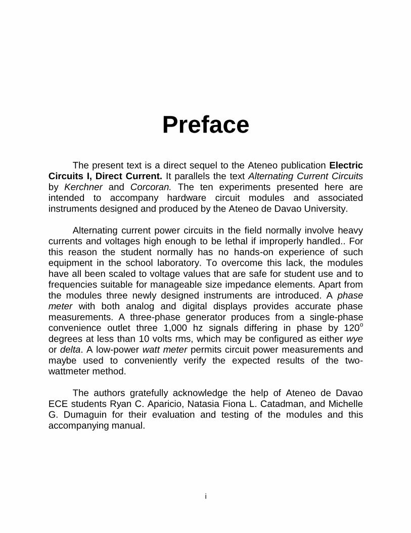
Preface
The present text is a direct sequel to the Ateneo publication Electric Circuits I, Direct Current. It parallels the text Alternating Current Circuits by Kerchner and Corcoran. The ten experiments presented here are intended to accompany hardware circuit modules and associated instruments designed and produced by the Ateneo de Davao University. Alternating current power circuits in the field normally involve heavy currents and voltages high enough to be lethal if improperly handled.. For this reason the student normally has no hands-on experience of such equipment in the school laboratory. To overcome this lack, the modules have all been scaled to voltage values that are safe for student use and to frequencies suitable for manageable size impedance elements. Apart from the modules three newly designed instruments are introduced. A phase meter with both analog and digital displays provides accurate phase measurements. A three-phase generator produces from a single-phase convenience outlet three 1,000 hz signals differing in phase by 120
o
degrees at less than 10 volts rms, which may be configured as either wye or delta. A low-power watt meter permits circuit power measurements and maybe used to conveniently verify the expected results of the two-wattmeter method. The authors gratefully acknowledge the help of Ateneo de Davao ECE students Ryan C. Aparicio, Natasia Fiona L. Catadman, and Michelle G. Dumaguin for their evaluation and testing of the modules and this accompanying manual.
ii
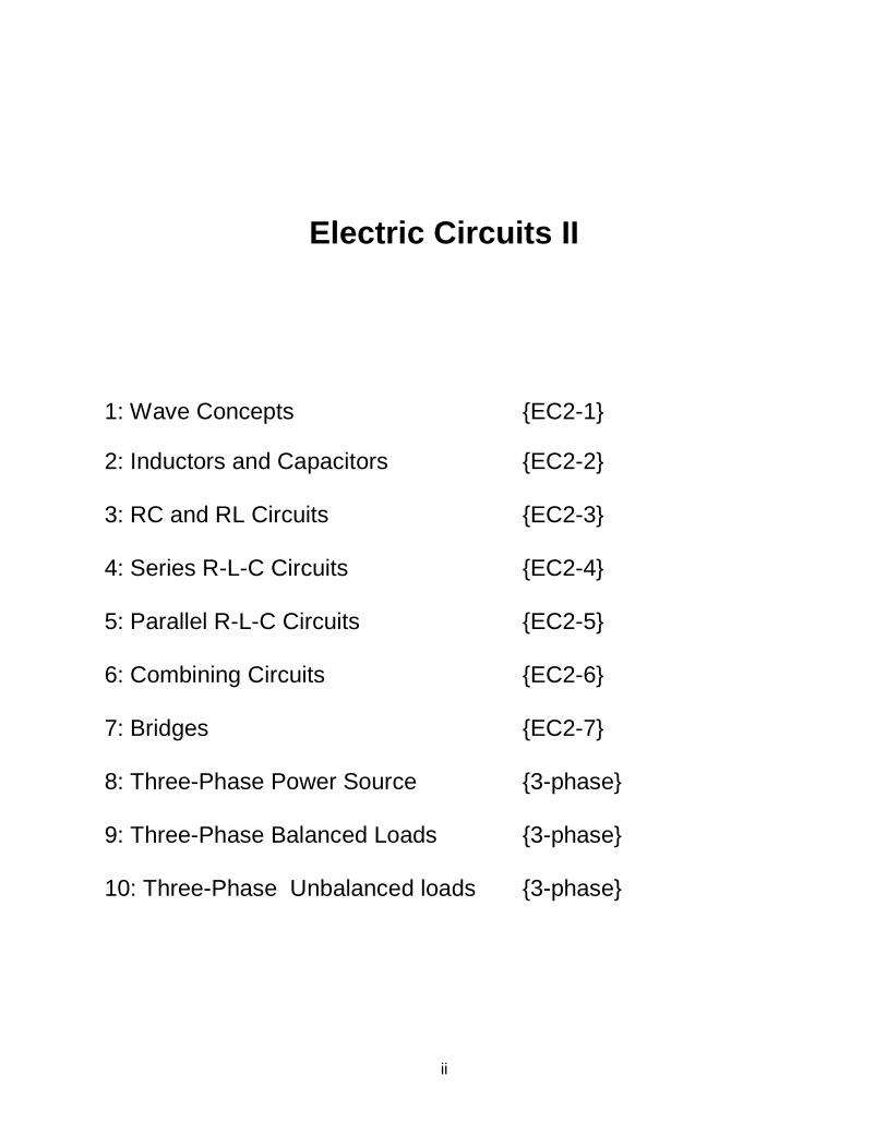
Electric Circuits II
1: Wave Concepts {EC2-1}
2: Inductors and Capacitors {EC2-2} 3: RC and RL Circuits {EC2-3} 4: Series R-L-C Circuits {EC2-4} 5: Parallel R-L-C Circuits {EC2-5} 6: Combining Circuits {EC2-6} 7: Bridges {EC2-7} 8: Three-Phase Power Source {3-phase} 9: Three-Phase Balanced Loads {3-phase} 10: Three-Phase Unbalanced loads {3-phase}
1 1: Wave Concepts
Wave Concepts
Equipment: Function Generator , Phase Shifter, Phase Meter. Oscilloscope
Sines and cosines (often lumped together as sinusoidal) are mathematical functions, the value of which depends on some other quantity, the argument. When used with triangles and vectors the argument is an angle, expressed in degrees or radians. When used to describe vibrating objects or electric currents the argument depends on time, and when used to describe wave motion (water, sound, radio or light) the argument is a particular combination of both position and time.
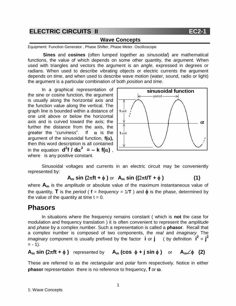
In a graphical representation of the sine or cosine function, the argument is usually along the horizontal axis and the function value along the vertical. The graph line is bounded within a distance of one unit above or below the horizontal axis and is curved toward the axis; the further the distance from the axis, the
greater the “curviness”. If is the
argument of the sinusoidal function, f(), then this word description is all contained
in the equation d2f / d
2 = – k f() ,
where is any positive constant. Sinusoidal voltages and currents in an electric circuit may be conveniently represented by:
Am sin (ft + ) or Am sin ((t/T + ) (1)
where Am is the amplitude or absolute value of the maximum instantaneous value of
the quantity, T is the period ( f = frequency = 1/T ) and is the phase, determined by
the value of the quantity at time t = 0.
Phasors
In situations where the frequency remains constant ( which is not the case for modulation and frequency translation ) it is often convenient to represent the amplitude and phase by a complex number. Such a representation is called a phasor. Recall that a complex number is composed of two components, the real and imaginary. The
imaginary component is usually prefixed by the factor i or j ( by definition i2 = j
2
= - 1).
Am sin (ft + ) represented by Am (cos + j sin ) or Am (2) These are referred to as the rectangular and polar form respectively. Notice in either
phasor representation there is no reference to frequency, f or
ELECTRIC CIRCUITS II EC2-1
2 1: Wave Concepts
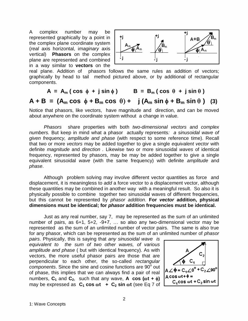
A complex number may be represented graphically by a point in the complex plane coordinate system (real axis horizontal, imaginary axis vertical) Phasors on the complex plane are represented and combined in a way similar to vectors on the real plane. Addition of phasors follows the same rules as addition of vectors; graphically by head to tail method pictured above, or by additional of rectangular components.
A = Am ( cos + j sin ) B = Bm ( cos + j sin )
A + B = (Am cos + Bm cos + j (Am sin + Bm sin ) (3)
Notice that phasors, like vectors, have magnitude and direction, and can be moved about anywhere on the coordinate system without a change in value. Phasors share properties with both two-dimensional vectors and complex numbers. But keep in mind what a phasor actually represents: a sinusoidal wave of given frequency, amplitude and phase (with respect to some reference time). Recall that two or more vectors may be added together to give a single equivalent vector with definite magnitude and direction . Likewise two or more sinusoidal waves of identical frequency, represented by phasors, may be may be added together to give a single equivalent sinusoidal wave (with the same frequency) with definite amplitude and phase. Although problem solving may involve different vector quantities as force and displacement, it is meaningless to add a force vector to a displacement vector, although these quantities may be combined in another way with a meaningful result. So also it is physically possible to combine together two sinusoidal waves of different frequencies, but this cannot be represented by phasor addition. For vector addition, physical dimensions must be identical; for phasor addition frequencies must be identical. Just as any real number, say 7, may be represented as the sum of an unlimited number of pairs, as 6+1, 5+2, -9+7, … so also any two-dimensional vector may be represented as the sum of an unlimited number of vector pairs. The same is also true for any phasor, which can be represented as the sum of an unlimited number of phasor pairs. Physically, this is saying that any sinusoidal wave is equivalent to the sum of two other waves, of various amplitude and phase ( but with identical frequency). As with vectors, the more useful phasor pairs are those that are perpendicular to each other, the so-called rectangular components. Since the sine and cosine functions are 90o out of phase, this implies that we can always find a pair of real
numbers, C1 and C2, such that any wave, A cos (t + )
may be expressed as C1 cos t + C2 sin t (see Eq 7 of

3 1: Wave Concepts
Notes on Trigonometry). For vectors, two forms of multiplication are defined, the dot and cross product. These are not applied to phasors. Multiplication of phasors follows the normal procedures for complex numbers (always recalling that j x j = j2 = –1
A B = [ Am (cos + j sin ) ] x [ Bm (cos + j sin ) ]
= AmBm[cos cos – sin sin j(cos sin + sin cos
which can be simplified by using Eqs. (7) and (9) from Notes on Trigonometry:
A B = AmBm [cos(+ ) + j sin(+ )] = AmBm + ). (4) So, for multiplication of phasors, multiply the magnitudes and add the angles. Since a phasor is basically a complex number, multiplication of a phasor by a complex number follows the example just above. This concept will be important as we extend Ohm’s Law for use with alternating currents.
Oscilloscope methods
We cannot see electricity and try to avoid, as far as possible, ever feeling it. Phasors and trigonometric expressions help us mentally picture its behavior. A cathode-ray oscilloscope produces a real-time voltage display. Other time-varying quantities may also be displayed, provided they are converted to voltage by a suitable transducer.
The display screen of a typical oscilloscope is 8 by 10 centimeters. Vertical displacements of the moving spot represent the input voltage, with selectable amplification settings in discrete steps from 20 volts / cm to 1 microvolt / cm. The input voltage may be fed to the vertical amplifier either directly or through an input capacitor. The oscilloscope may be used as a multi-range DC or AC voltmeter .
Horizontal spot displacements represent time, with a scale typically varying in discrete steps from a few seconds per centimeter to one microsecond per centimeter or less. Even with fixed settings for voltage and time, the trace placement may be positioned anywhere on the screen by adjusting the vertical position and horizontal position knobs. The oscilloscope may also be used as a multi-range frequency meter.
4 1: Wave Concepts
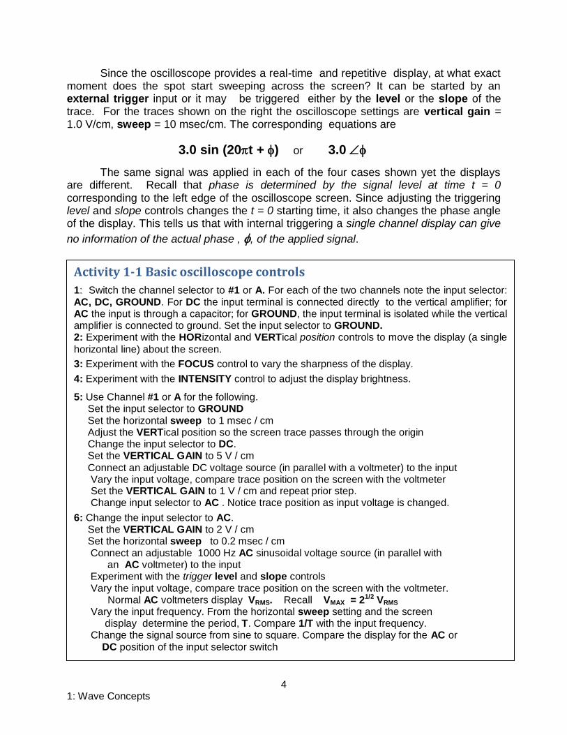
Since the oscilloscope provides a real-time and repetitive display, at what exact moment does the spot start sweeping across the screen? It can be started by an external trigger input or it may be triggered either by the level or the slope of the trace. For the traces shown on the right the oscilloscope settings are vertical gain = 1.0 V/cm, sweep = 10 msec/cm. The corresponding equations are
3.0 sin (20t + ) or 3.0
The same signal was applied in each of the four cases shown yet the displays are different. Recall that phase is determined by the signal level at time t = 0 corresponding to the left edge of the oscilloscope screen. Since adjusting the triggering level and slope controls changes the t = 0 starting time, it also changes the phase angle of the display. This tells us that with internal triggering a single channel display can give
no information of the actual phase , , of the applied signal.
Activity 1-1 Basic oscilloscope controls
1: Switch the channel selector to #1 or A. For each of the two channels note the input selector: AC, DC, GROUND. For DC the input terminal is connected directly to the vertical amplifier; for AC the input is through a capacitor; for GROUND, the input terminal is isolated while the vertical amplifier is connected to ground. Set the input selector to GROUND. 2: Experiment with the HORizontal and VERTical position controls to move the display (a single
horizontal line) about the screen.
3: Experiment with the FOCUS control to vary the sharpness of the display.
4: Experiment with the INTENSITY control to adjust the display brightness.
5: Use Channel #1 or A for the following. Set the input selector to GROUND Set the horizontal sweep to 1 msec / cm Adjust the VERTical position so the screen trace passes through the origin Change the input selector to DC. Set the VERTICAL GAIN to 5 V / cm
Connect an adjustable DC voltage source (in parallel with a voltmeter) to the input Vary the input voltage, compare trace position on the screen with the voltmeter Set the VERTICAL GAIN to 1 V / cm and repeat prior step. Change input selector to AC . Notice trace position as input voltage is changed.
6: Change the input selector to AC. Set the VERTICAL GAIN to 2 V / cm Set the horizontal sweep to 0.2 msec / cm
Connect an adjustable 1000 Hz AC sinusoidal voltage source (in parallel with an AC voltmeter) to the input Experiment with the trigger level and slope controls
Vary the input voltage, compare trace position on the screen with the voltmeter. Normal AC voltmeters display VRMS. Recall VMAX = 21/2 VRMS Vary the input frequency. From the horizontal sweep setting and the screen display determine the period, T. Compare 1/T with the input frequency. Change the signal source from sine to square. Compare the display for the AC or DC position of the input selector switch
5 1: Wave Concepts
Dual-channel display
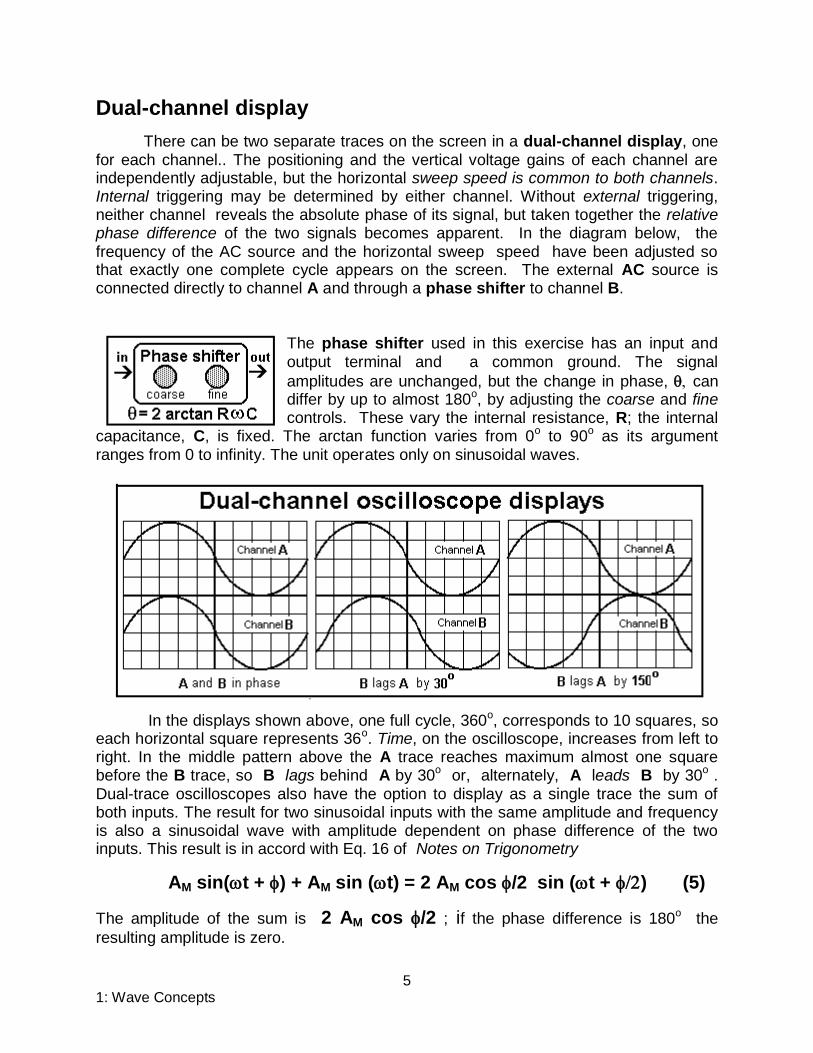
There can be two separate traces on the screen in a dual-channel display, one for each channel.. The positioning and the vertical voltage gains of each channel are independently adjustable, but the horizontal sweep speed is common to both channels. Internal triggering may be determined by either channel. Without external triggering, neither channel reveals the absolute phase of its signal, but taken together the relative phase difference of the two signals becomes apparent. In the diagram below, the frequency of the AC source and the horizontal sweep speed have been adjusted so that exactly one complete cycle appears on the screen. The external AC source is connected directly to channel A and through a phase shifter to channel B.
The phase shifter used in this exercise has an input and output terminal and a common ground. The signal
amplitudes are unchanged, but the change in phase, can differ by up to almost 180o, by adjusting the coarse and fine controls. These vary the internal resistance, R; the internal
capacitance, C, is fixed. The arctan function varies from 0o to 90o as its argument ranges from 0 to infinity. The unit operates only on sinusoidal waves.
In the displays shown above, one full cycle, 360o, corresponds to 10 squares, so each horizontal square represents 36o. Time, on the oscilloscope, increases from left to right. In the middle pattern above the A trace reaches maximum almost one square before the B trace, so B lags behind A by 30o or, alternately, A leads B by 30o . Dual-trace oscilloscopes also have the option to display as a single trace the sum of both inputs. The result for two sinusoidal inputs with the same amplitude and frequency is also a sinusoidal wave with amplitude dependent on phase difference of the two inputs. This result is in accord with Eq. 16 of Notes on Trigonometry
AM sin(t + ) + AM sin (t) = 2 AM cos /2 sin (t + ) (5)
The amplitude of the sum is 2 AM cos /2 ; if the phase difference is 180o the
resulting amplitude is zero.
6 1: Wave Concepts
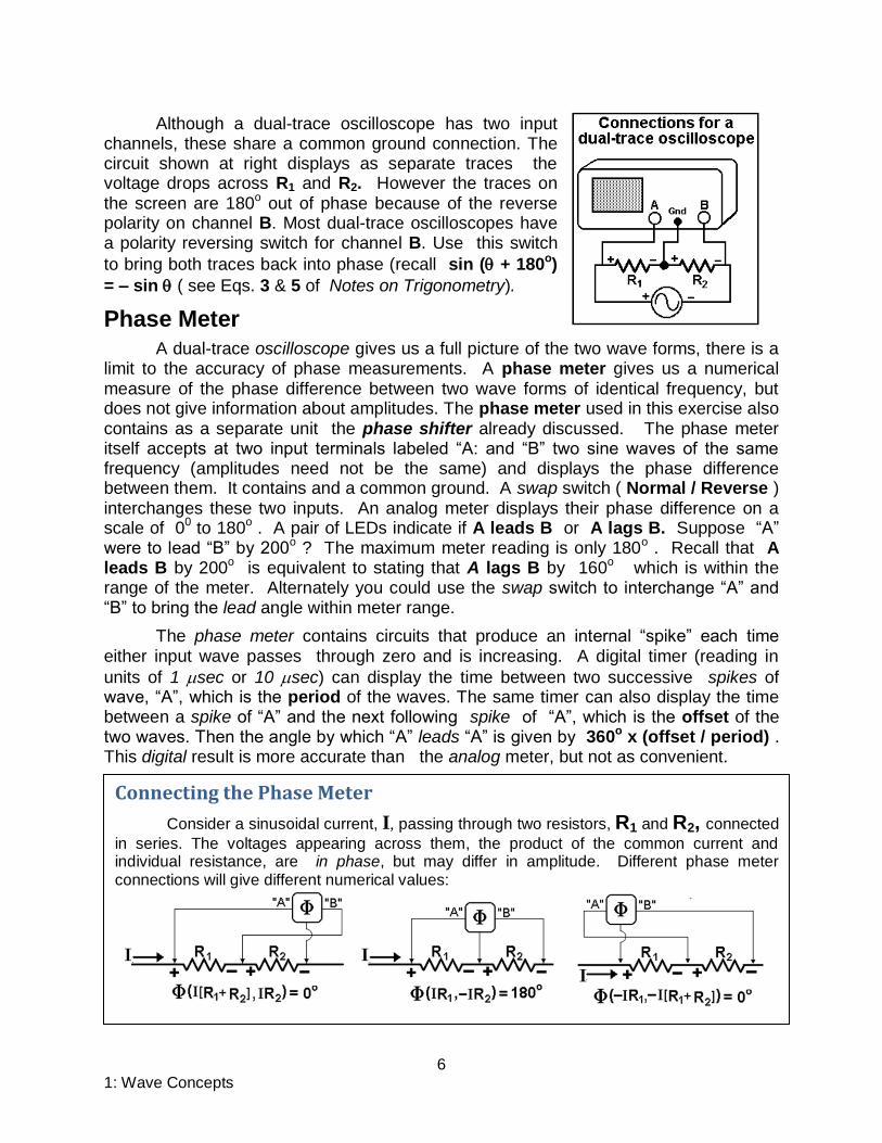
Although a dual-trace oscilloscope has two input channels, these share a common ground connection. The circuit shown at right displays as separate traces the voltage drops across R1 and R2. However the traces on the screen are 180o out of phase because of the reverse polarity on channel B. Most dual-trace oscilloscopes have a polarity reversing switch for channel B. Use this switch
to bring both traces back into phase (recall sin ( + 180o)
= – sin ( see Eqs. 3 & 5 of Notes on Trigonometry).
Phase Meter
A dual-trace oscilloscope gives us a full picture of the two wave forms, there is a limit to the accuracy of phase measurements. A phase meter gives us a numerical measure of the phase difference between two wave forms of identical frequency, but does not give information about amplitudes. The phase meter used in this exercise also contains as a separate unit the phase shifter already discussed. The phase meter itself accepts at two input terminals labeled “A: and “B” two sine waves of the same frequency (amplitudes need not be the same) and displays the phase difference between them. It contains and a common ground. A swap switch ( Normal / Reverse ) interchanges these two inputs. An analog meter displays their phase difference on a scale of 0
0 to 180
o . A pair of LEDs indicate if A leads B or A lags B. Suppose “A”
were to lead “B” by 200o ? The maximum meter reading is only 180o . Recall that A leads B by 200o is equivalent to stating that A lags B by 160o which is within the range of the meter. Alternately you could use the swap switch to interchange “A” and “B” to bring the lead angle within meter range.
The phase meter contains circuits that produce an internal “spike” each time either input wave passes through zero and is increasing. A digital timer (reading in
units of 1 sec or 10 sec) can display the time between two successive spikes of wave, “A”, which is the period of the waves. The same timer can also display the time between a spike of “A” and the next following spike of “A”, which is the offset of the two waves. Then the angle by which “A” leads “A” is given by 360o x (offset / period) . This digital result is more accurate than the analog meter, but not as convenient.
Connecting the Phase Meter
Consider a sinusoidal current, I, passing through two resistors, R1 and R2, connected
in series. The voltages appearing across them, the product of the common current and individual resistance, are in phase, but may differ in amplitude. Different phase meter connections will give different numerical values:

7 1: Wave Concepts
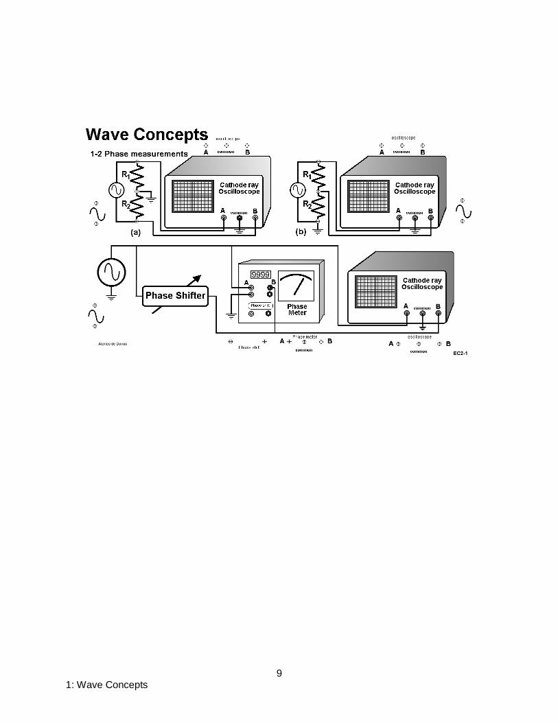
Activity 1- 2 Oscilloscope phase measurements
1: Connect a function generator to the dual-trace oscilloscope, as shown in (a). Use a sine
wave, approximately 1 kHz, five volts peak-to-peak. Let R1 = R2 = any convenient value. Set oscilloscope input selector to AC, VERTICAL GAIN to 1 V/cm. ,SWEEP to 0.5 m/sec/cm and display mode to DUAL
2: Adjust the VERTical POSition control of each channel so no part of the traces overlap.
Change the setting of the polarity-reversing switch for channel B and observe traces. Switch the display mode to ADD and observe traces.
3: Connect the circuit as shown in (b) and repeat the activity of step 2
4: Reconnect the circuit as shown just above with the phase meter and oscilloscope in
parallel. Note that the phase shifter is a part of the phase meter module. Adjust the phase shifter for minimum phase difference between the two traces and observe the display and the readings of the phase meter and calculate the phase difference, in degrees.
5: Again adjust the phase shifter so the two traces differ by just ¼ wavelength. Note the
phase meter readings. Change the phase meter SWAP between normal and reverse and note any change in display or meter readings.
6: Set to maximum the COARSE and FINE controls of the phase shifter. Note the new
phase meter readings. Without changing the phase shifter controls, set the input frequency to 1, 2, 3 and measure the amount of phase shift. new phase meter readings.
The relation = 2 arctan RC may also be expressed as (tan /2)/(2f) =
RC From the data above calculate the probable value of RC

8 1: Wave Concepts
Data Sheet Experiment # EC2-1 Wave Concepts
Name ______________________________ Date__________
Activity 1-2: Oscilloscope phase measurements
With circuit (a): Swap switch normal : Waves in phase? _______ Swap switch reverse : Waves in phase? _______
With circuit (b): Swap switch normal : Waves in phase? _______ Swap switch reverse : Waves in phase? _______ Describe the effect of the ADD switch for waves in-phase and 180o out-of-phase __________________________________________________________________
________________________________________________________ Step 5: Swap switch normal: offset / period ___________ Swap switch reverse: offset / period ___________
frequency phase angle (tan /2)/(2f)
1,000
2,000
3,000
4,000
9 1: Wave Concepts

2: Inductors and Capacitors 10
Inductors and Capacitors
Equipment: Function Generator , Wattmeter, Phase Shifter, Phase Meter. Oscilloscope
An electric circuit is an array of interconnected active and passive elements capable of transferring electromagnetic energy. Active elements supply energy to the circuit; passive elements either store electromagnetic energy (inductors and capacitors) or transform it to another form of energy (resistors, motors, LEDs…). Within the circuit, energy is transferred whenever electric charge moves (current) moves through a potential difference (voltage). In a course on Alternating Current Circuits, attention is focused on the resistor, inductor and capacitor. All are passive, two-terminal elements. Current may pass through the terminals (no net charge is stored in these elements) and a difference in potential may exist between the terminals. If the current flows into the terminal at higher potential and out of the terminal at lower potential (always the case for a resistor) the element absorbs energy from the circuit; if the current is in the other direction the element returns stored energy to the circuit.
The Inductor An inductor stores energy in its magnetic field produced by the current flowing through it; changing the current changes the stored energy just as changing the speed of a moving object changes its stored kinetic energy. To transfer energy in or out there must also be a potential difference across the inductor terminals. If no potential difference then no energy transfer. For a given rate of change in current the potential difference across the terminals depends on the characteristics of the inductor, known as inductance, usually represented by the letter L.
(potential difference) = L (rate of current change) : v = L di/dt (1)
The physical dimensions of inductance are volts /(amperes / second) or henry. If one volt appears across the inductor terminals as the current through it is changing at a rate of one ampere per second, the inductance is one henry.
ELECTRIC CIRCUITS II EC2-2

2: Inductors and Capacitors 11
Consider the case in which the instantaneous current through the inductor, i(t),
is sinusoidal: i(t) = Im sin t . From Eq. (1) the instantaneous voltage, v(t) must be
v(t) = L di/dt = L Im d(sin t)/dt
v(t) = Im L cos t = Vm cos t (2)
where Vm = ImL . Since both i(t) and v(t) are sinusoidal the peak values, Im and
Vm may be replaces by their root-mean-square values (as read by a multimeter),
VRMS = IRMS L (2a)
Impedance
If the current through a resistor, R, is expressed as i(t) = Im sin t , then by
Ohm’s law the voltage across the resistor is given by vR(t) = Im R sin t ; the current
and voltage are in phase. But for an inductor, carrying the same current, the voltage
across it , by Eq. (2), is vL(t) = Im L cos t; here the current and voltage are 90o
out of phase. Here is where the concept of the impedance of an passive circuit element is useful:
Activity 2-1: Inductor sinusoidal response
Equation (2a) may be written as IRMS = VRMS / f L . In this activity you are
to verify this relationship. The current , IRMS, is measured as either VRMS , f or L alone
is changed.
1: Use the approximate settings of f = 1.000 khz, L = 40.0 mh and V = 1,1.5, 2,
2.5, 3 and measure the corresponding current, I , and compare with V/ 2fL .
2: Use the approximate settings of f = 2.000 khz, V = 3 v and L = 40, 50, 60, 70, 80
mh and measure the corresponding current, I , and compare with V/ 2fL
3: Use the approximate settings of V = 2.00 v, L = 50.0 mh and f= 0.5, 1, 1.5, 2, 2.5
khz and measure the corresponding current, I , and compare with V/ 2fL .
.
(voltage across element) = IMPEDANCE x (current through element) (3)
2: Inductors and Capacitors 12
IMPEDANCE = (Resistance) + j (Reactance)
Z = R + jX
= (R2 + X
2) where = tan
–1 (X/R)
impedance of an ideal inductor = 0 + j L
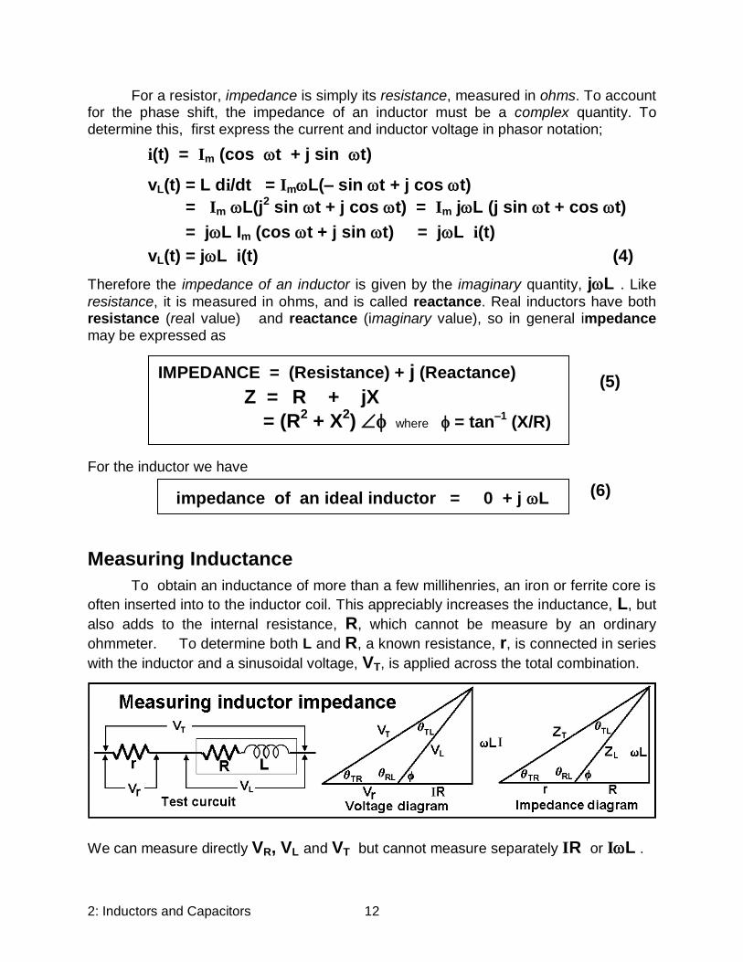
For a resistor, impedance is simply its resistance, measured in ohms. To account for the phase shift, the impedance of an inductor must be a complex quantity. To determine this, first express the current and inductor voltage in phasor notation;
i(t) = Im (cos t + j sin t)
vL(t) = L di/dt = ImL(– sin t + j cos t)
= Im L(j2 sin t + j cos t) = Im jL (j sin t + cos t)
= jL Im (cos t + j sin t) = jL i(t)
vL(t) = jL i(t) (4)
Therefore the impedance of an inductor is given by the imaginary quantity, jL . Like
resistance, it is measured in ohms, and is called reactance. Real inductors have both resistance (real value) and reactance (imaginary value), so in general impedance may be expressed as
(5)
For the inductor we have
(6)
Measuring Inductance
To obtain an inductance of more than a few millihenries, an iron or ferrite core is
often inserted into to the inductor coil. This appreciably increases the inductance, L, but
also adds to the internal resistance, R, which cannot be measure by an ordinary
ohmmeter. To determine both L and R, a known resistance, r, is connected in series
with the inductor and a sinusoidal voltage, VT, is applied across the total combination.
We can measure directly VR, VL and VT but cannot measure separately IR or IL .
2: Inductors and Capacitors 13
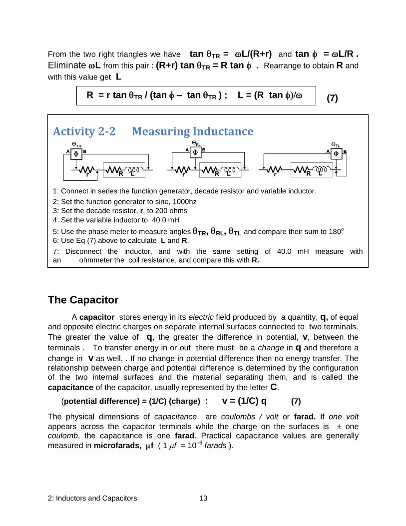
R = r tan TR / (tan – tan TR ) ; L = (R tan
From the two right triangles we have tan TR = L/(R+r) and tan = L/R .
Eliminate L from this pair : (R+r) tan TR = R tan . Rearrange to obtain R and
with this value get L
(7)
The Capacitor
A capacitor stores energy in its electric field produced by a quantity, q, of equal
and opposite electric charges on separate internal surfaces connected to two terminals.
The greater the value of q, the greater the difference in potential, v, between the
terminals . To transfer energy in or out there must be a change in q and therefore a
change in v as well. . If no change in potential difference then no energy transfer. The
relationship between charge and potential difference is determined by the configuration of the two internal surfaces and the material separating them, and is called the
capacitance of the capacitor, usually represented by the letter C.
(potential difference) = (1/C) (charge) : v = (1/C) q (7)
The physical dimensions of capacitance are coulombs / volt or farad. If one volt
appears across the capacitor terminals while the charge on the surfaces is one coulomb, the capacitance is one farad. Practical capacitance values are generally
measured in microfarads, f ( 1 f = 10–6 farads ).
Activity 2-2 Measuring Inductance
1: Connect in series the function generator, decade resistor and variable inductor.
2: Set the function generator to sine, 1000hz
3: Set the decade resistor, r, to 200 ohms
4: Set the variable inductor to 40.0 mH
5: Use the phase meter to measure angles TR, RL, TL and compare their sum to 180o
6: Use Eq (7) above to calculate L and R.
7: Disconnect the inductor, and with the same setting of 40.0 mH measure with
an ohmmeter the coil resistance, and compare this with R.
2: Inductors and Capacitors 14
impedance of a capacitor = 0 – j (1/C)
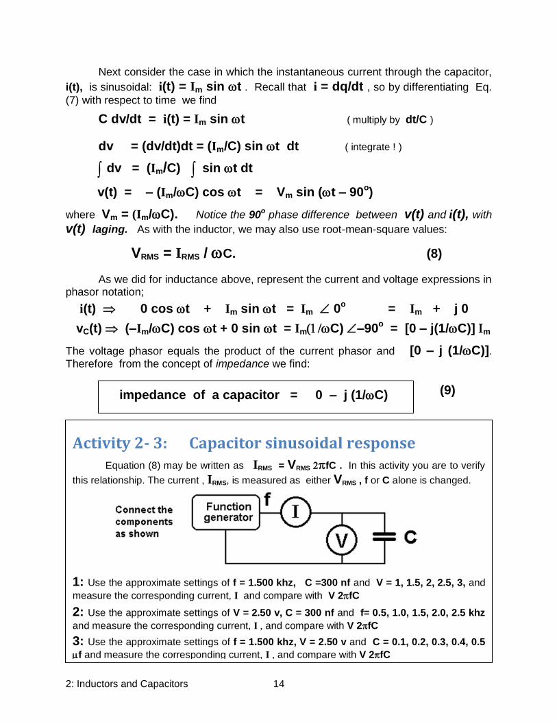
Activity 2- 3: Capacitor sinusoidal response
Equation (8) may be written as IRMS = VRMS fC . In this activity you are to verify
this relationship. The current , IRMS, is measured as either VRMS , f or C alone is changed.
1: Use the approximate settings of f = 1.500 khz, C =300 nf and V = 1, 1.5, 2, 2.5, 3, and
measure the corresponding current, I and compare with V 2fC
2: Use the approximate settings of V = 2.50 v, C = 300 nf and f= 0.5, 1.0, 1.5, 2.0, 2.5 khz
and measure the corresponding current, I , and compare with V 2fC
3: Use the approximate settings of f = 1.500 khz, V = 2.50 v and C = 0.1, 0.2, 0.3, 0.4, 0.5
f and measure the corresponding current, I , and compare with V 2fC
Next consider the case in which the instantaneous current through the capacitor,
i(t), is sinusoidal: i(t) = Im sin t . Recall that i = dq/dt , so by differentiating Eq.
(7) with respect to time we find
C dv/dt = i(t) = Im sin t ( multiply by dt/C )
dv = (dv/dt)dt = (Im/C) sin t dt ( integrate ! )
dv = (Im/C) sin t dt
v(t) = – (Im/C) cos t = Vm sin (t – 90o)
where Vm = (Im/C). Notice the 90o phase difference between v(t) and i(t), with
v(t) laging. As with the inductor, we may also use root-mean-square values:
VRMS = IRMS / C. (8)
As we did for inductance above, represent the current and voltage expressions in phasor notation;
i(t) 0 cos t + Im sin t = Im 0o = Im + j 0
vC(t) (–Im/C) cos t + 0 sin t = ImC) –90o = [0 – j(1/C)] m
The voltage phasor equals the product of the current phasor and [0 – j (1/C)]. Therefore from the concept of impedance we find:
(9)
2: Inductors and Capacitors 15
R = r tan TR / (tan – tan TR ) ; C = 1/(Rtan
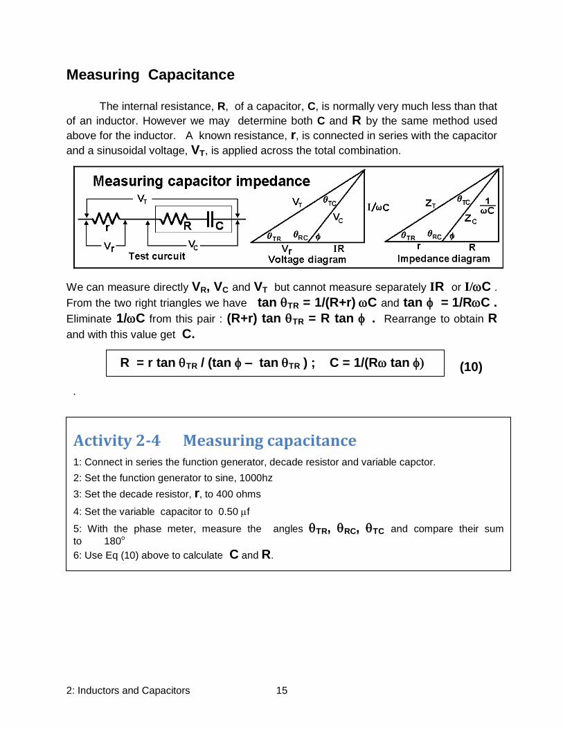
Measuring Capacitance The internal resistance, R, of a capacitor, C, is normally very much less than that
of an inductor. However we may determine both C and R by the same method used
above for the inductor. A known resistance, r, is connected in series with the capacitor
and a sinusoidal voltage, VT, is applied across the total combination.
We can measure directly VR, VC and VT but cannot measure separately IR or I/C .
From the two right triangles we have tan TR = 1/(R+r)C and tan = 1/RC .
Eliminate 1/C from this pair : (R+r) tan TR = R tan . Rearrange to obtain R
and with this value get C.
(10)
.
Activity 2-4 Measuring capacitance
1: Connect in series the function generator, decade resistor and variable capctor.
2: Set the function generator to sine, 1000hz
3: Set the decade resistor, r, to 400 ohms
4: Set the variable capacitor to 0.50 f
5: With the phase meter, measure the angles TR, RC, TC and compare their sum
to 180o
6: Use Eq (10) above to calculate C and R.
2: Inductors and Capacitors 16
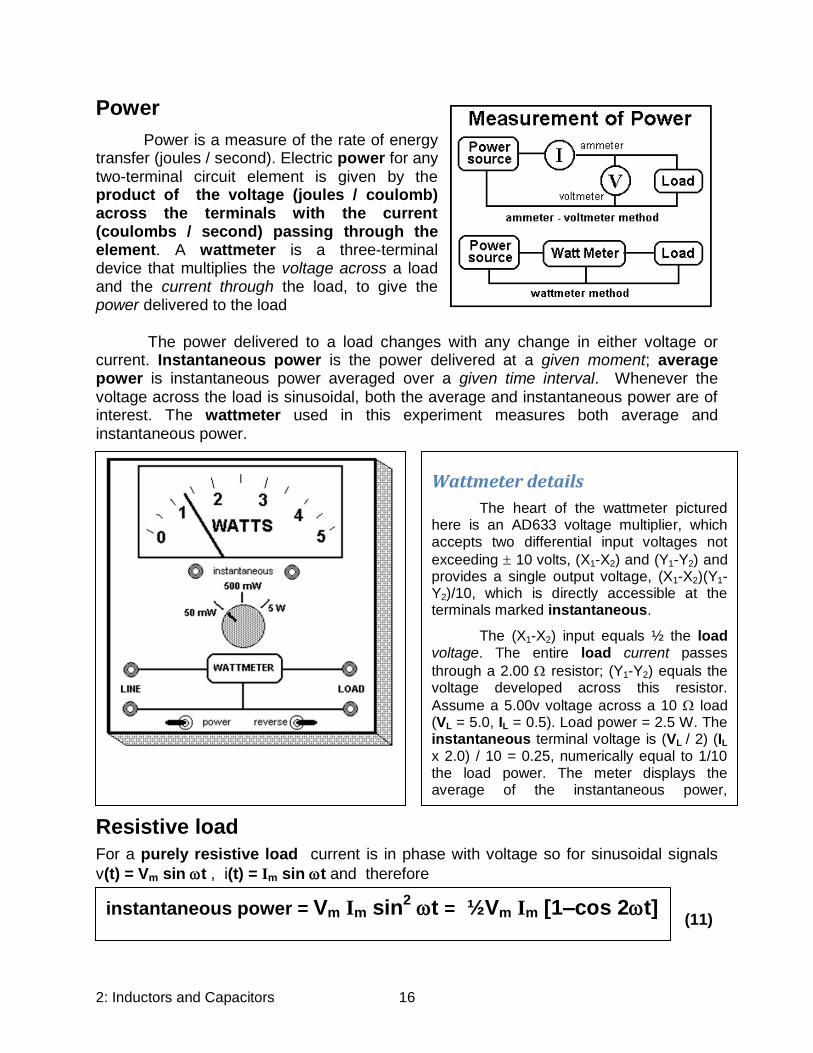
Wattmeter details
The heart of the wattmeter pictured here is an AD633 voltage multiplier, which accepts two differential input voltages not
exceeding 10 volts, (X1-X2) and (Y1-Y2) and provides a single output voltage, (X1-X2)(Y1-Y2)/10, which is directly accessible at the terminals marked instantaneous.
The (X1-X2) input equals ½ the load voltage. The entire load current passes
through a 2.00 resistor; (Y1-Y2) equals the voltage developed across this resistor.
Assume a 5.00v voltage across a 10 load (VL = 5.0, IL = 0.5). Load power = 2.5 W. The instantaneous terminal voltage is (VL / 2) (IL
x 2.0) / 10 = 0.25, numerically equal to 1/10 the load power. The meter displays the average of the instantaneous power, multiplied by a selected range factor
instantaneous power = Vm Im sin2 t = ½Vm Im [1–cos 2t]
Power
Power is a measure of the rate of energy transfer (joules / second). Electric power for any two-terminal circuit element is given by the product of the voltage (joules / coulomb) across the terminals with the current (coulombs / second) passing through the element. A wattmeter is a three-terminal device that multiplies the voltage across a load and the current through the load, to give the power delivered to the load The power delivered to a load changes with any change in either voltage or current. Instantaneous power is the power delivered at a given moment; average power is instantaneous power averaged over a given time interval. Whenever the voltage across the load is sinusoidal, both the average and instantaneous power are of interest. The wattmeter used in this experiment measures both average and instantaneous power.
Resistive load
For a purely resistive load current is in phase with voltage so for sinusoidal signals
v(t) = Vm sin t , i(t) = Im sin t and therefore
(11)
2: Inductors and Capacitors 17
average power = ½ Vm Im
average power = Vrms Irms
using Eq. (12a) of Notes on Trigonometry. Since the average value of cos 2t is zero, (12)
Oscilloscope screens display voltage amplitudes, Vm, while conventional multimeters display root-mean-square values, Vrms , which are related as
Vm = 21/2
Vrms and Im = 21/2
Irms (13)
Substituting (13) into (12) gives
(14)
Since rms values are never negative, for a purely resistive load the average power can never be negative. Also, since the magnitude of the cosine term is never greater than 1.0, Eq. (11) indicate that the instantaneous power can never be negative.
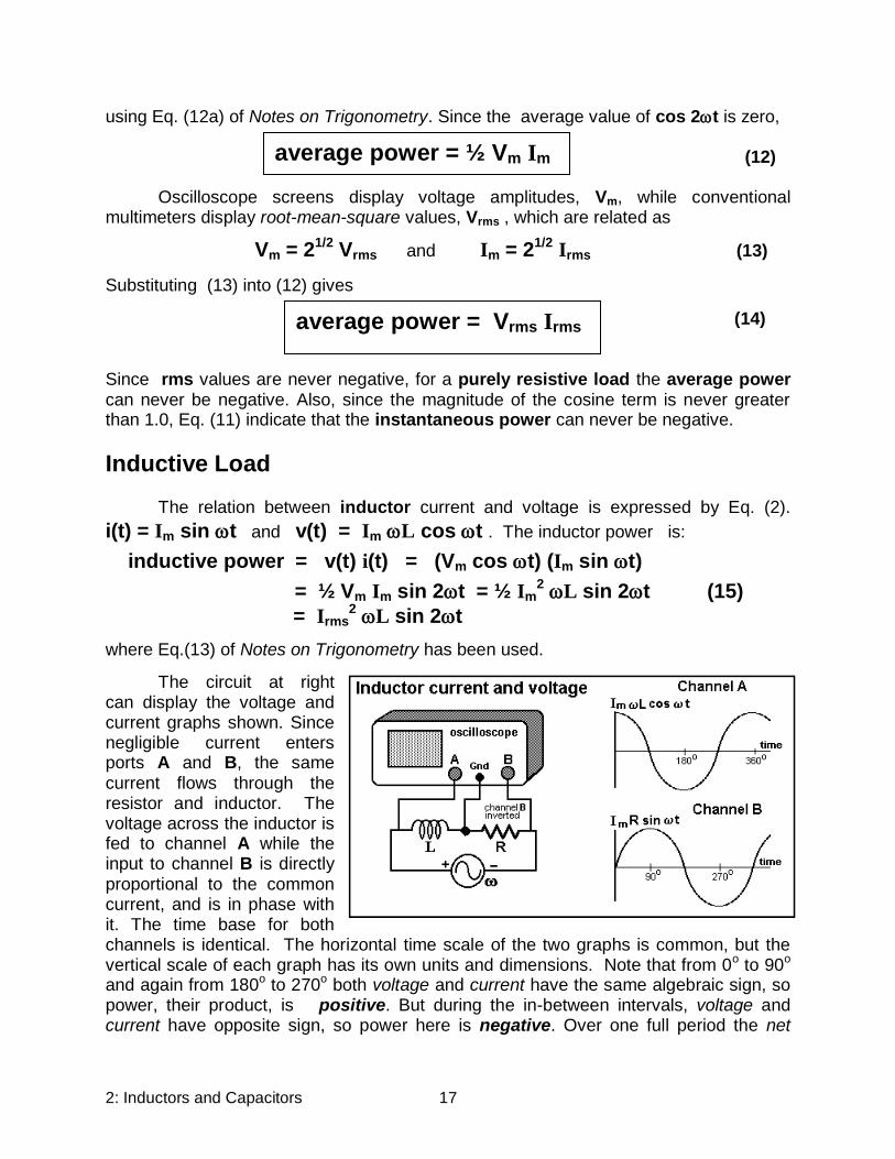
Inductive Load The relation between inductor current and voltage is expressed by Eq. (2). i(t) = Im sin t and v(t) = Im L cos t . The inductor power is:
inductive power = v(t) i(t) = (Vm cos t) (Im sin t)
= ½ Vm Im sin 2t = ½ Im2 L sin 2t (15)
= Irms2 L sin 2t
where Eq.(13) of Notes on Trigonometry has been used.
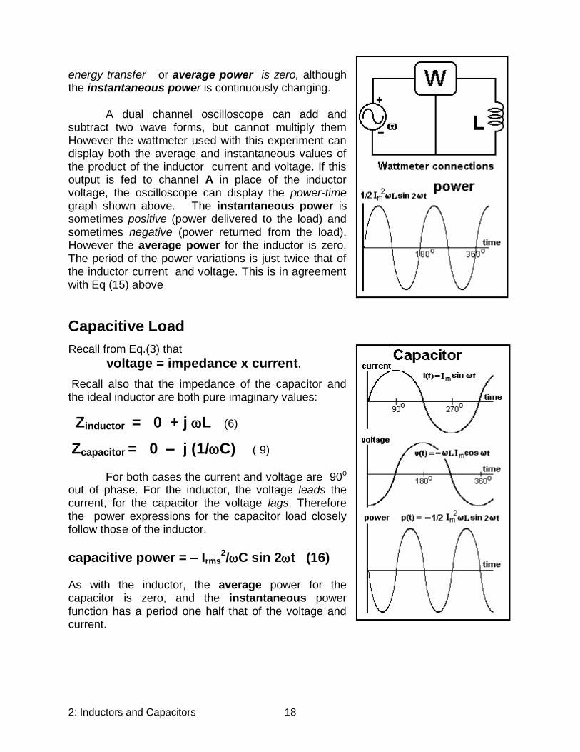
The circuit at right can display the voltage and current graphs shown. Since negligible current enters ports A and B, the same current flows through the resistor and inductor. The voltage across the inductor is fed to channel A while the input to channel B is directly proportional to the common current, and is in phase with it. The time base for both channels is identical. The horizontal time scale of the two graphs is common, but the vertical scale of each graph has its own units and dimensions. Note that from 0o to 90o and again from 180o to 270o both voltage and current have the same algebraic sign, so power, their product, is positive. But during the in-between intervals, voltage and current have opposite sign, so power here is negative. Over one full period the net
2: Inductors and Capacitors 18
energy transfer or average power is zero, although the instantaneous power is continuously changing. A dual channel oscilloscope can add and subtract two wave forms, but cannot multiply them However the wattmeter used with this experiment can display both the average and instantaneous values of the product of the inductor current and voltage. If this output is fed to channel A in place of the inductor voltage, the oscilloscope can display the power-time graph shown above. The instantaneous power is sometimes positive (power delivered to the load) and sometimes negative (power returned from the load). However the average power for the inductor is zero. The period of the power variations is just twice that of the inductor current and voltage. This is in agreement with Eq (15) above
Capacitive Load
Recall from Eq.(3) that
voltage = impedance x current.
Recall also that the impedance of the capacitor and the ideal inductor are both pure imaginary values:
Zinductor = 0 + j L (6)
Zcapacitor = 0 – j (1/C) ( 9)
For both cases the current and voltage are 90o
out of phase. For the inductor, the voltage leads the current, for the capacitor the voltage lags. Therefore the power expressions for the capacitor load closely follow those of the inductor.
capacitive power = – Irms2/C sin 2t (16)
As with the inductor, the average power for the capacitor is zero, and the instantaneous power function has a period one half that of the voltage and current.
2: Inductors and Capacitors 19
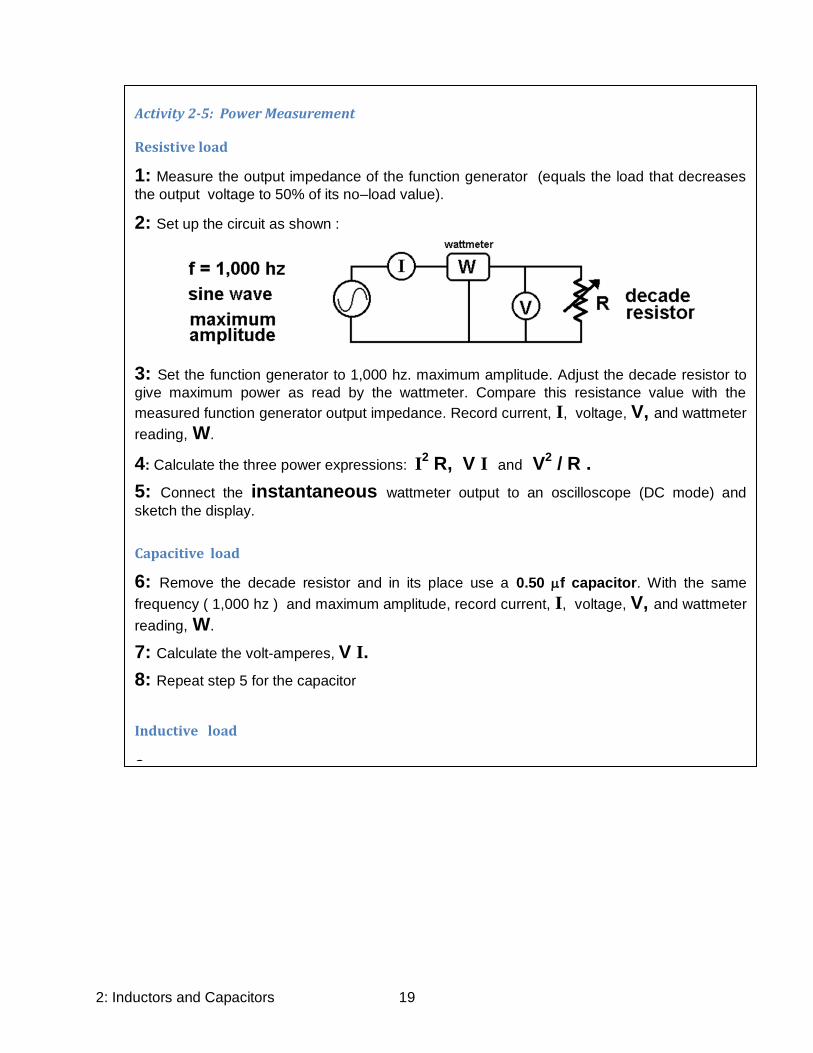
Activity 2-5: Power Measurement
Resistive load
1: Measure the output impedance of the function generator (equals the load that decreases
the output voltage to 50% of its no–load value).
2: Set up the circuit as shown :
3: Set the function generator to 1,000 hz. maximum amplitude. Adjust the decade resistor to
give maximum power as read by the wattmeter. Compare this resistance value with the
measured function generator output impedance. Record current, I, voltage, V, and wattmeter
reading, W.
4: Calculate the three power expressions: I2 R, V I and V
2 / R .
5: Connect the instantaneous wattmeter output to an oscilloscope (DC mode) and
sketch the display.
Capacitive load
6: Remove the decade resistor and in its place use a 0.50 f capacitor. With the same
frequency ( 1,000 hz ) and maximum amplitude, record current, I, voltage, V, and wattmeter
reading, W.
7: Calculate the volt-amperes, V I.
8: Repeat step 5 for the capacitor
Inductive load
9: Repeat steps 6, 7, 8 for an inductive load of 50 mH
2: Inductors and Capacitors 20
Data Sheet Experiment # EC2-2 Inductors and Capacitors
Name ______________________________ Date__________
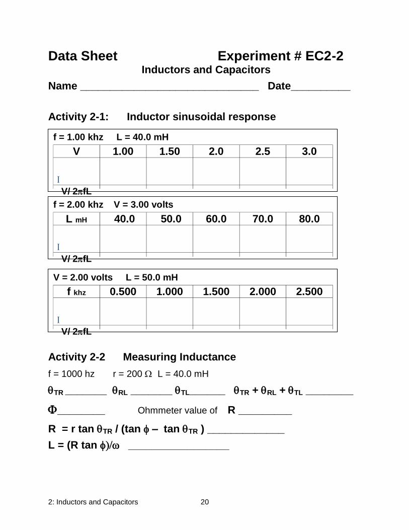
Activity 2-1: Inductor sinusoidal response
Activity 2-2 Measuring Inductance
f = 1000 hz r = 200 L = 40.0 mH
TR _______ RL _______ TL______ TR + RL + TL ________
________ Ohmmeter value of R _________
R = r tan TR / (tan – tan TR ) _____________
L = (R tan _________________
f = 1.00 khz L = 40.0 mH
V 1.00 1.50 2.0 2.5 3.0
I
V/ 2fL
f = 2.00 khz V = 3.00 volts
L mH 40.0 50.0 60.0 70.0 80.0
I
V/ 2fL
V = 2.00 volts L = 50.0 mH
f khz 0.500 1.000 1.500 2.000 2.500
I
V/ 2fL

2: Inductors and Capacitors 21
Data Sheet Experiment # EC2-2 (continued) Activity 2- 3: Capacitor sinusoidal response
Activity 2-4 Measuring Capacitance
f = 1000 hz r = 400 C = 500 nf
TR _______ RC _______ TC______ TR + RC + TC ________
________
R = r tan TR / (tan – tan TR ) _______________
C = 1/(Rtan
f = 1.500 khz C = 300 nf
V 1.00 1.50 2.0 2.5 3.0 I
V 2fC
V = 2.50 volts C = 300 nf
f hz 500 1000 1500 2000 2500 I
V 2fC
V = 2.50 volts f = 1500 hz
C nf 100 200 300 400 500 I
V 2fC

2: Inductors and Capacitors 22
Data Sheet Experiment # EC2-2 (continued)
Activity 2-5: Power Measurement
Resistive load
Source output impedance _______
I ______ V _______ R _______
I2 R ________ V I ________
V2 / R _______ W ________
Sweep = 0.1 mSec /cm Vertical = 20 mV / cm
Capacitive load
I ______ V _______
W _______
V I ________
Sweep = 0.1 mSec /cm Vertical = _____________
Inductive load
I ______ V _______
W _______
V I ________
Sweep = 0.1 mSec /cm Vertical = _____________
2: Inductors and Capacitors 23
3: RC and RL circuits 24
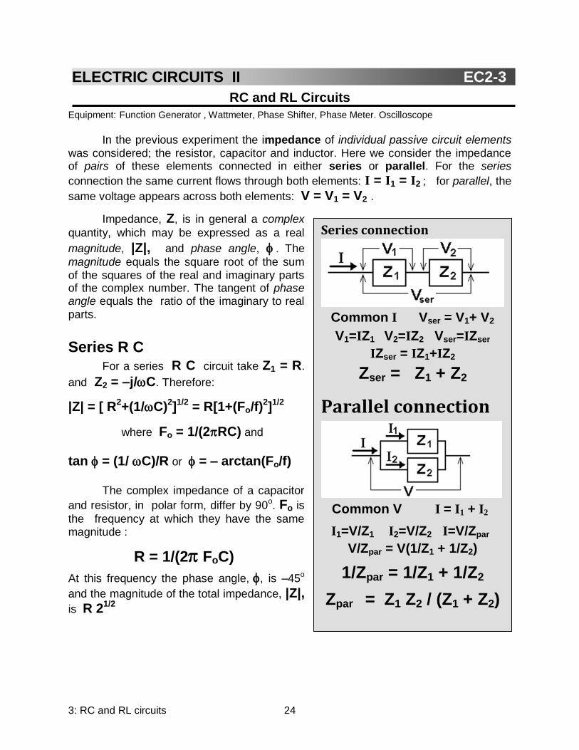
Series connection
Common I Vser = V1+ V2
V1=IZ1 V2=IZ2 Vser=IZser
IZser = IZ1+IZ2
Zser = Z1 + Z2
Parallel connection
Common V I = I1 + I2
I1=V/Z1 I2=V/Z2 I=V/Zpar
V/Zpar = V(1/Z1 + 1/Z2)
1/Zpar = 1/Z1 + 1/Z2
Zpar = Z1 Z2 / (Z1 + Z2)
RC and RL Circuits
Equipment: Function Generator , Wattmeter, Phase Shifter, Phase Meter. Oscilloscope
In the previous experiment the impedance of individual passive circuit elements was considered; the resistor, capacitor and inductor. Here we consider the impedance of pairs of these elements connected in either series or parallel. For the series
connection the same current flows through both elements: I = I1 = I2 ; for parallel, the
same voltage appears across both elements: V = V1 = V2 .
Impedance, Z, is in general a complex
quantity, which may be expressed as a real
magnitude, |Z|, and phase angle, The
magnitude equals the square root of the sum of the squares of the real and imaginary parts of the complex number. The tangent of phase angle equals the ratio of the imaginary to real parts.
Series R C
For a series R C circuit take Z1 = R.
and Z2 = –j/C. Therefore:
|Z| = [ R2+(1/C)
2]1/2
= R[1+(Fo/f)2]1/2
where Fo = 1/(2RC) and
tan = (1/ C)/R or = – arctan(Fo/f) The complex impedance of a capacitor
and resistor, in polar form, differ by 90o. Fo is
the frequency at which they have the same magnitude :
R = 1/(2 FoC)
At this frequency the phase angle,, is –45o
and the magnitude of the total impedance, |Z|, is R 2
1/2
ELECTRIC CIRCUITS II EC2-3

3: RC and RL circuits 25
The above normalized diagrams show that when f = Fo the value of |Z|/R is
21/2 or 1.4 and the phase angle, , is 45o . For f 0 the value of |Z|/R increases
without limit due to the series capacitor. As f ∞ the value of |Z|/R approaches 1.0, for
a very high frequencies the impedance of the capacitor may be neglected in comparison with R.
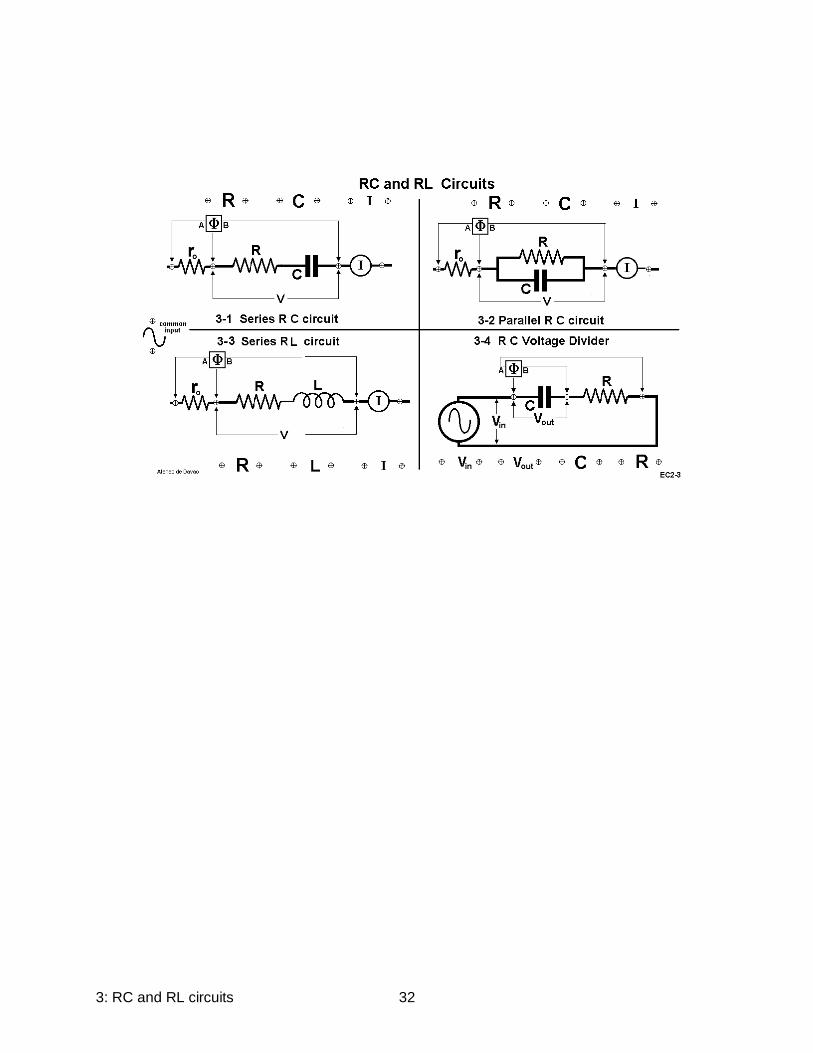
Activity 3-1 Series R C circuit
1: Connect R, C, ro, and the AC voltmeter, ammeter and phase meter and function
generator as shown above. Select R as 500 ohms, C as 500 nano-farads (1 nf = 1.0x10⁻⁹
farads) and ro about five hundred ohms. ( |Z| is independent of ro ; the voltage across ro
is used only as a phase meter reference. In this configuration the phase meter reading,
, differs from , the phase difference between V and I, by 180o ). The function generator
frequency may be determined from the period setting of the phase meter ( 5,000 sec
period corresponds to 200.0 hertz)
2: Adjust the function generator for a period in the neighborhood of seven thousand
microseconds, sine wave, maximum amplitude. Measure and record V and I (in milli-
amperes) from the multimeters and the period and offset (in micro-
3: RC and RL circuits 26
Parallel R C
For a parallel combination of a resistor and capacitor we may easily guess the outcome; at low frequencies the capacitor impedance is many times greater than the R of the resistor in parallel, so the resulting impedance is due to R alone, so |Z|/R ≈ 1. At very high frequencies the capacitor impedance is quite low, effectively short-circuiting
the parallel resistor, so |Z|/R 0
R L Circuits The analysis of R L circuits is quite similar to that of R C circuits already
considered. The complex impedance of the inductor is 2 f L or L and the value
of Fo , the frequency at which | 2 f L | = R is given as Fo = R / 2 L .
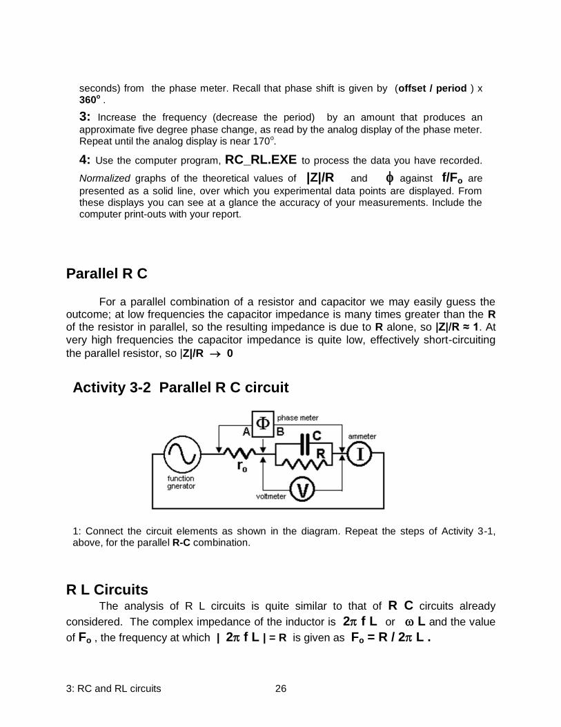
seconds) from the phase meter. Recall that phase shift is given by (offset / period ) x 360o .
3: Increase the frequency (decrease the period) by an amount that produces an
approximate five degree phase change, as read by the analog display of the phase meter. Repeat until the analog display is near 170o.
4: Use the computer program, RC_RL.EXE to process the data you have recorded.
Normalized graphs of the theoretical values of |Z|/R and against f/Fo are
presented as a solid line, over which you experimental data points are displayed. From these displays you can see at a glance the accuracy of your measurements. Include the computer print-outs with your report.
Activity 3-2 Parallel R C circuit
1: Connect the circuit elements as shown in the diagram. Repeat the steps of Activity 3-1, above, for the parallel R-C combination.
3: RC and RL circuits 27
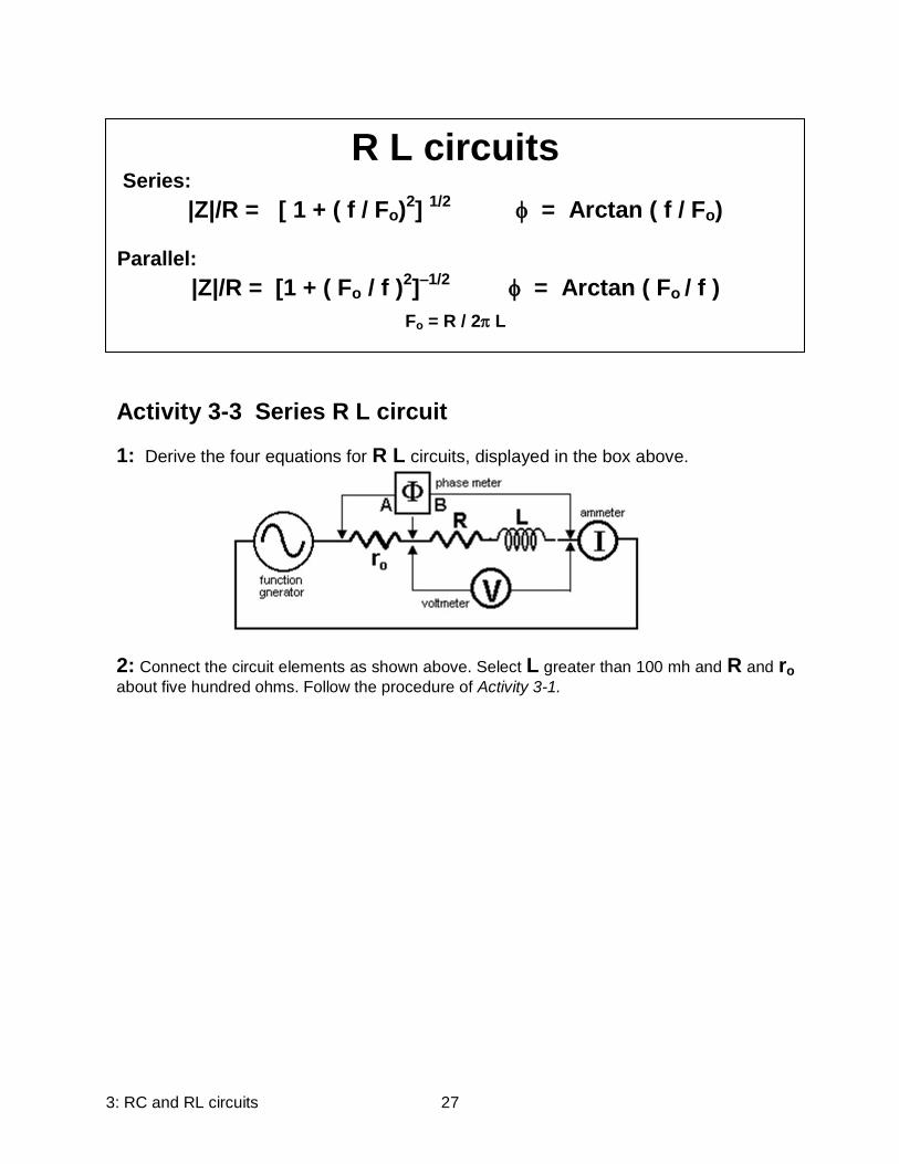
R L circuits Series:
|Z|/R = [ 1 + ( f / Fo)2]
1/2 = Arctan ( f / Fo)
Parallel:
|Z|/R = [1 + ( Fo / f )2]–1/2
= Arctan ( Fo / f )
Fo = R / 2 L
Activity 3-3 Series R L circuit
1: Derive the four equations for R L circuits, displayed in the box above.
2: Connect the circuit elements as shown above. Select L greater than 100 mh and R and ro about five hundred ohms. Follow the procedure of Activity 3-1.
3: RC and RL circuits 28
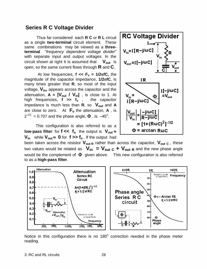
Series R C Voltage Divider
Thus far considered each R C or R L circuit as a single two-terminal circuit element. These same combinations may be viewed as a three-terminal “frequency dependent voltage divider” with separate input and output voltages. In the
circuit shown at right It is assumed that Vout is
open, so the same current flows through R and C.
At low frequencies, f << Fo = 1/2fC, the
magnitude of the capacitor impedance, 1/2fC, is many times greater that R, so most of the input
voltage, Vin, appears across the capacitor and the
attenuation, A = |Vout / Vin| , is close to 1. At
high frequencies, f >> fo , the capacitor
impedance is much less than R, so Vout and A
are close to zero. At Fo the attenuation, A , is
2-1/2 = 0.707 and the phase angle, , is –45o.
This configuration is also referred to as a
low-pass filter: for f << fo the output is Vout
Vin while Vout 0 for f >> fo . If the output had
been taken across the resistor Vout R rather than across the capacitor, Vout C , these
two values would be related as Vin = Vout C + Vout R and the new phase angle
would be the complement of given above. This new configuration is also referred
to as a high-pass filter.
Notice in this configuration there is no 180o correction needed in the phase meter reading.
3: RC and RL circuits 29
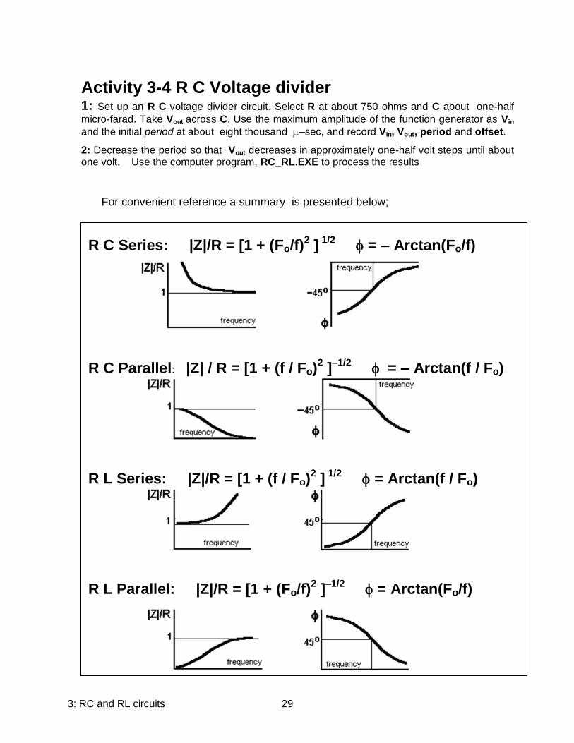
For convenient reference a summary is presented below;
Activity 3-4 R C Voltage divider
1: Set up an R C voltage divider circuit. Select R at about 750 ohms and C about one-half
micro-farad. Take Vout across C. Use the maximum amplitude of the function generator as Vin
and the initial period at about eight thousand –sec, and record Vin, Vout, period and offset.
2: Decrease the period so that Vout decreases in approximately one-half volt steps until about one volt. Use the computer program, RC_RL.EXE to process the results
R C Series: |Z|/R = [1 + (Fo/f)2 ]
1/2 = – Arctan(Fo/f)
R C Parallel: |Z| / R = [1 + (f / Fo)
2 ]
–1/2 = – Arctan(f / Fo)
R L Series: |Z|/R = [1 + (f / Fo)
2 ]
1/2 = Arctan(f / Fo)
R L Parallel: |Z|/R = [1 + (Fo/f)
2 ]
–1/2 = Arctan(Fo/f)
3: RC and RL circuits 30
V Volts
I m Amps
Period -sec
Offset -sec
V Volts
I m Amps
Period -sec
Offset -sec
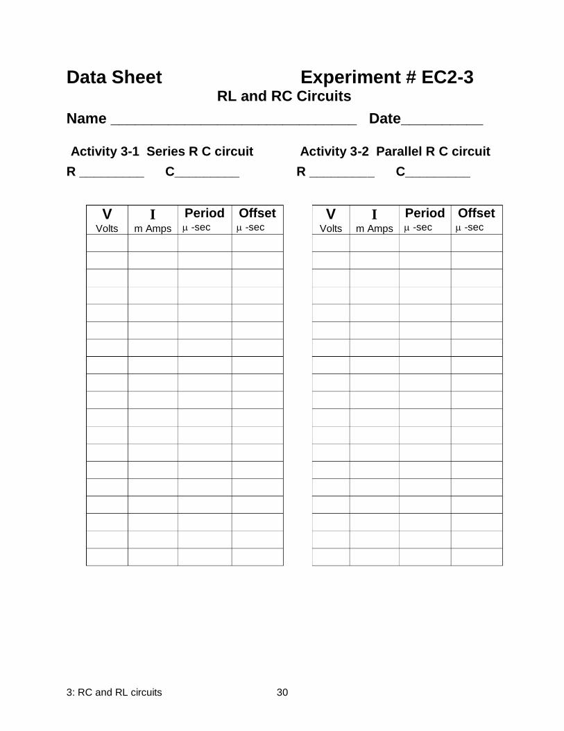
Data Sheet Experiment # EC2-3 RL and RC Circuits
Name ______________________________ Date__________
Activity 3-1 Series R C circuit Activity 3-2 Parallel R C circuit
R _________ C_________ R _________ C_________
3: RC and RL circuits 31
V Volts
I m Amps
Period -sec
Offset -sec
Vin Volts
Vout Volts
Period -sec
Offset -sec
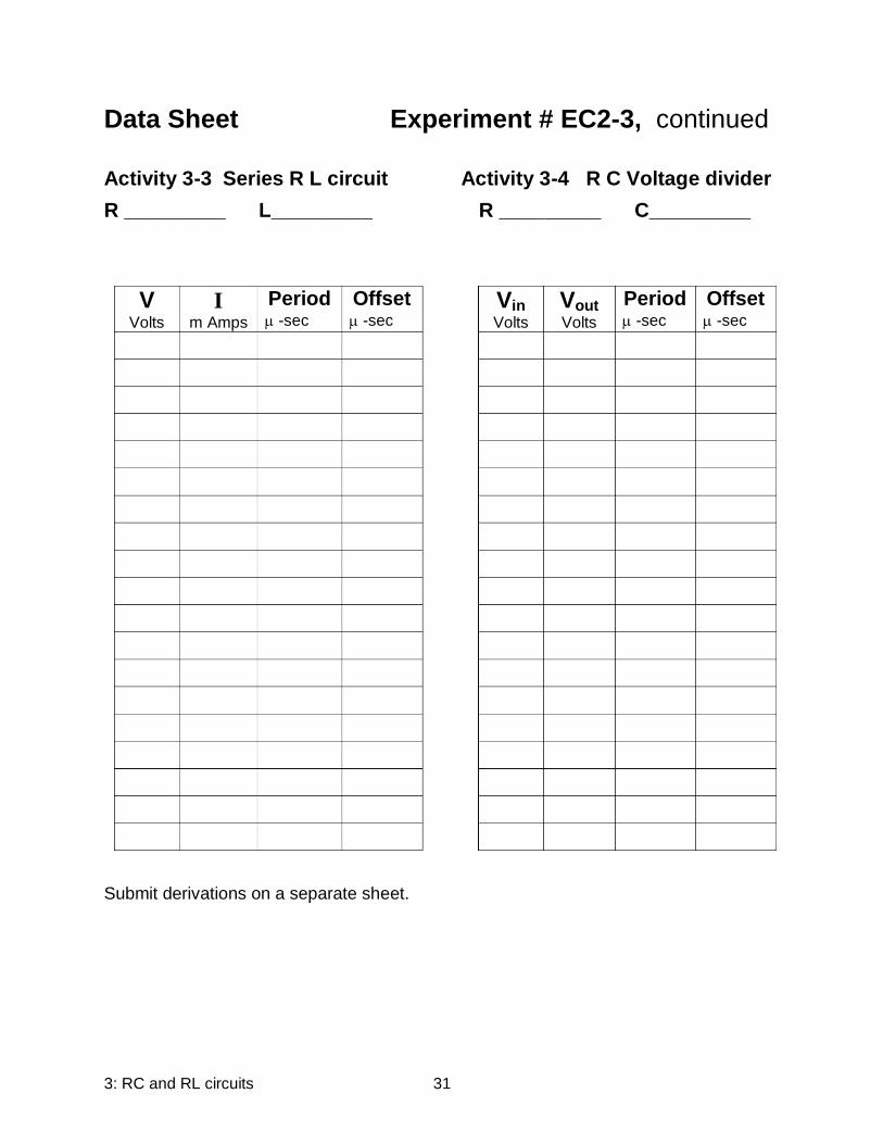
Data Sheet Experiment # EC2-3, continued
Activity 3-3 Series R L circuit Activity 3-4 R C Voltage divider
R _________ L_________ R _________ C_________
Submit derivations on a separate sheet.
3: RC and RL circuits 32
4: Series R-L-C Circuits 33
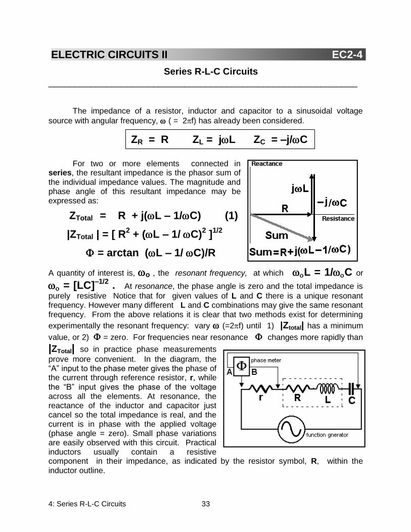
Series R-L-C Circuits ___________________________________________________________ The impedance of a resistor, inductor and capacitor to a sinusoidal voltage
source with angular frequency, ( = 2f) has already been considered.
For two or more elements connected in series, the resultant impedance is the phasor sum of the individual impedance values. The magnitude and phase angle of this resultant impedance may be expressed as:
ZTotal = R + j(L – 1/C) (1)
|ZTotal | = [ R2 + (L – 1/C)
2 ]
1/2
= arctan (L – 1/C)/R
A quantity of interest is, o , the resonant frequency, at which L = 1/C or
= [LC]–1/2
. At resonance, the phase angle is zero and the total impedance is
purely resistive Notice that for given values of L and C there is a unique resonant frequency. However many different L and C combinations may give the same resonant frequency. From the above relations it is clear that two methods exist for determining
experimentally the resonant frequency: vary (=2f) until 1) |Ztotal| has a minimum
value, or 2) = zero. For frequencies near resonance changes more rapidly than
|ZTotal| so in practice phase measurements
prove more convenient. In the diagram, the “A” input to the phase meter gives the phase of the current through reference resistor, r, while the “B” input gives the phase of the voltage across all the elements. At resonance, the reactance of the inductor and capacitor just cancel so the total impedance is real, and the current is in phase with the applied voltage (phase angle = zero). Small phase variations are easily observed with this circuit. Practical inductors usually contain a resistive component in their impedance, as indicated by the resistor symbol, R, within the inductor outline.
ELECTRIC CIRCUITS II EC2-4
ZR = R ZL = jL ZC = –j/C

4: Series R-L-C Circuits 34
Inductor resistance
In Activity 2 of Experiment EL2-2 the resistive component of an inductor’s impedance was measured using a right-triangle impedance diagram. A series resonant circuit provides an alternate method to measure this same value. At series resonance the combined reactance of the capacitor and inductor is zero. Assuming the capacitor resistance is quite small, the voltage
drop across the series resonant circuit is VT .
The external series resistor, r, is used to
calculate the series current, I = Vr / r . The
inductor resistance, R, follows from these
values. Below 100 kHz, the copper resistance of the coil windings does not appreciably change with frequency. Magnetic core material is often used in used to increase dramatically the inductance of the coil windings alone. The magnetic field of the inductor current causes the microscopic magnetic domains of the steel or ferrite core to orient themselves with this field but some “friction” in involved. This adds significantly to the total field but also requires energy. The higher the frequency, the more frequently these domains are rotated and more energy is required. This results in an increase of
resistance, for electric energy is converted into heat ( power = energy / time = I2R )
whenever a current passes through a resistor. If the “inductor” is the field windings of an electric motor, or the coil of a loud-speaker, an additional resistive component
Activity 4-1 Verify the relation = [LC]–1/2
For a given L and C, measure fo (=o/2)
1: Set up the circuit as shown above. Set r = 100.0 .Use the L and C values indicated on
the Data Sheet. Adjust the input signal frequency to give a zero phase angle, as measured by the phase meter and record the corresponding frequency, fo Compare this
with[2LC]
–1/2.
For a given value of L and fo , measure the corresponding value for C
2: Set the input signal to 1000 hz. Use the same circuit configuration as in step 1 above. With the values of L shown on the data sheet, adjust C to give a zero phase angle.
Note: If the signal amplitude to too large or too small the phase meter digital readings
become erratic. Therefore adjust the amplitude accordingly.
4: Series R-L-C Circuits 35
appears, since mechanical or sound energy is provided by the device.
“Quality” of a series resonant circuit
Notice at resonance a one volt input signal, VT. can produce an inductor or
capacitor voltage, VL or VC of five, ten or more volts. This voltage multiplication is one
measure of the “quality”, Q, of a series resonant circuit, defined as
where = [LC]–1/2
. Q has no physical dimensions. It a property of the whole series
resonant circuit, although It is also common practice to speak of the Q of the inductor
alone assuming it is in series with a capacitor C such that C = 1/(L2) .
The total impedance of a series R-L-C circuit is given by Eq. 1. Just at
resonance (f = fo , =o) the capacitive and inductive reactance are equal, XL = XC,
so the circuit total impedance is R alone and the current , I, is VT / R. The individual
capacitor and inductor voltages may be expressed as:
|VC| = I|ZCI = IXC = I (1/C) and |VC /VT|= 1/(RC) = Q
|VL| = I|ZL| = I[R2 + (L)
2]1/2
and |VL/VT| = [1+(L/R)2]1/2
= [1+Q2]1/2
The two voltage ratios are measured by the circuit “quality”, Q. To maximize Q for a
series R-L-C circuit with fixed resonant frequency, , decrease R and C and increase
L ( but keep constant the LC product, . From the prior activity we saw that the L
value of an inductor increases with the square of the number of turns (more resistance in the wire) and with the properties of the core material (effective resistance of increasing core losses) . To obtain a practical maximum Q, trade-offs are necessary.
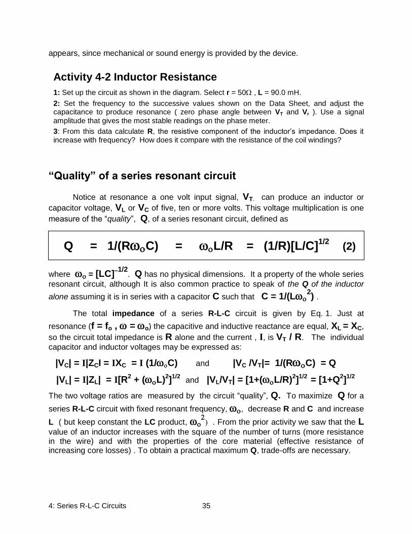
Activity 4-2 Inductor Resistance
1: Set up the circuit as shown in the diagram. Select r = 50 , L = 90.0 mH.
2: Set the frequency to the successive values shown on the Data Sheet, and adjust the capacitance to produce resonance ( zero phase angle between VT and Vr ). Use a signal
amplitude that gives the most stable readings on the phase meter.
3: From this data calculate R, the resistive component of the inductor’s impedance. Does it increase with frequency? How does it compare with the resistance of the coil windings?
Q = 1/(RC) = L/R = (1/R)[L/C]1/2
(2)
4: Series R-L-C Circuits 36
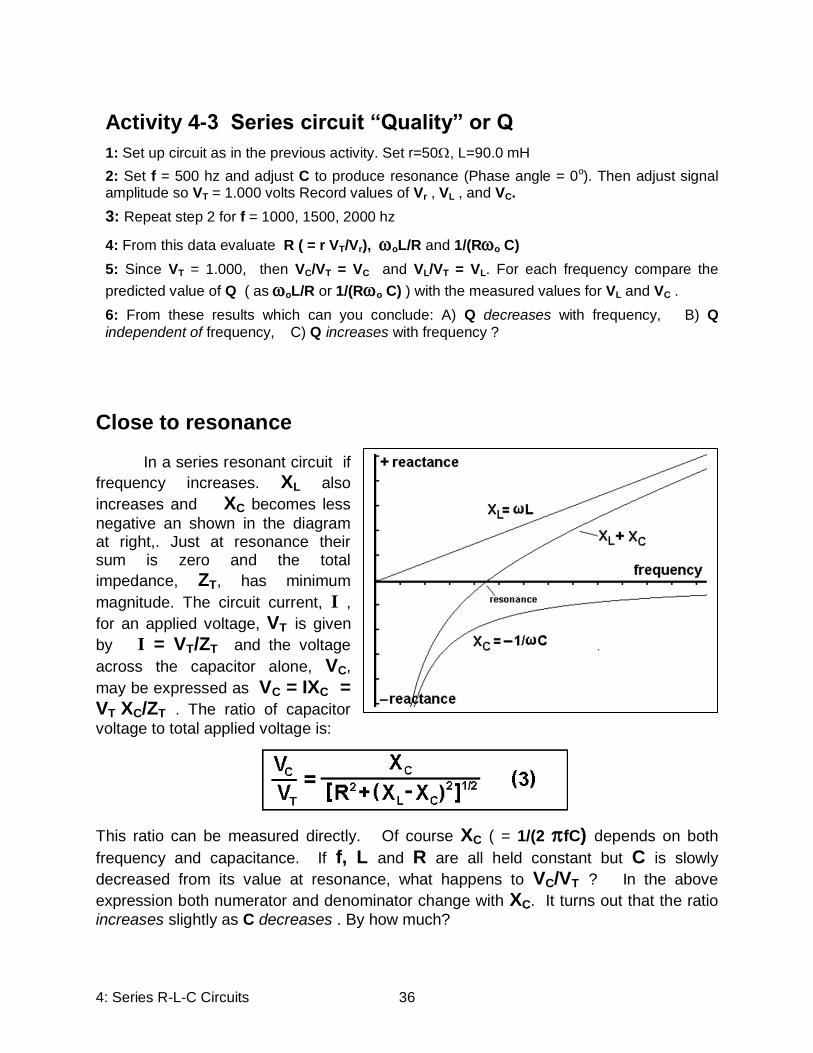
Close to resonance
In a series resonant circuit if
frequency increases. XL also
increases and XC becomes less
negative an shown in the diagram at right,. Just at resonance their sum is zero and the total
impedance, ZT, has minimum
magnitude. The circuit current, I ,
for an applied voltage, VT is given
by I = VT/ZT and the voltage
across the capacitor alone, VC,
may be expressed as VC = IXC = VT XC/ZT . The ratio of capacitor
voltage to total applied voltage is:
This ratio can be measured directly. Of course XC ( = 1/(2 fC) depends on both
frequency and capacitance. If f, L and R are all held constant but C is slowly
decreased from its value at resonance, what happens to VC/VT ? In the above
expression both numerator and denominator change with XC. It turns out that the ratio
increases slightly as C decreases . By how much?
Activity 4-3 Series circuit “Quality” or Q
1: Set up circuit as in the previous activity. Set r=50, L=90.0 mH
2: Set f = 500 hz and adjust C to produce resonance (Phase angle = 0o). Then adjust signal amplitude so VT = 1.000 volts Record values of Vr , VL , and VC.
3: Repeat step 2 for f = 1000, 1500, 2000 hz
4: From this data evaluate R ( = r VT/Vr), oL/R and 1/(Ro C)
5: Since VT = 1.000, then VC/VT = VC and VL/VT = VL. For each frequency compare the
predicted value of Q ( as oL/R or 1/(Ro C) ) with the measured values for VL and VC .
6: From these results which can you conclude: A) Q decreases with frequency, B) Q
independent of frequency, C) Q increases with frequency ?
4: Series R-L-C Circuits 37
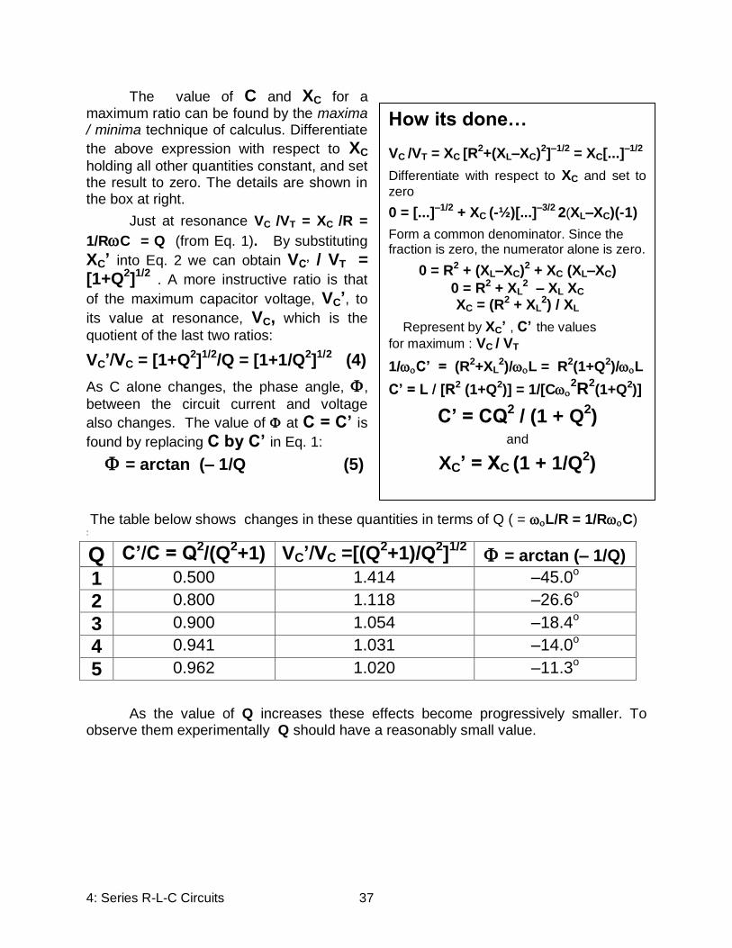
How its done…
VC /VT = XC [R2+(XL–XC)2]–1/2 = XC[...]–1/2
Differentiate with respect to XC and set to
zero
0 = [...]–1/2 + XC (-½)[...]–3/2 2(XL–XC)(-1)
Form a common denominator. Since the fraction is zero, the numerator alone is zero.
0 = R2 + (XL–XC)2 + XC (XL–XC)
0 = R2 + XL2 – XL XC
XC = (R2 + XL2) / XL
Represent by XC’ , C’ the values
for maximum : VC / VT
1/C’ = (R2+XL2)/L = R2(1+Q2)/L
C’ = L / [R2 (1+Q2)] = 1/[C2R
2(1+Q2)]
C’ = CQ2 / (1 + Q
2)
and
XC’ = XC (1 + 1/Q2)
The value of C and XC for a maximum ratio can be found by the maxima / minima technique of calculus. Differentiate
the above expression with respect to XC holding all other quantities constant, and set the result to zero. The details are shown in the box at right.
Just at resonance VC /VT = XC /R =
1/RC = Q (from Eq. 1). By substituting
XC’ into Eq. 2 we can obtain VC’ / VT = [1+Q
2]1/2
. A more instructive ratio is that
of the maximum capacitor voltage, VC’, to
its value at resonance, VC, which is the
quotient of the last two ratios:
VC’/VC = [1+Q2]1/2
/Q = [1+1/Q2]1/2
(4)
As C alone changes, the phase angle, ,
between the circuit current and voltage
also changes. The value of at C = C’ is
found by replacing C by C’ in Eq. 1:
= arctan (– 1/Q (5)
The table below shows changes in these quantities in terms of Q ( = L/R = 1/RC) :
Q C’/C = Q2/(Q
2+1) VC’/VC =[(Q
2+1)/Q
2]1/2
= arctan (– 1/Q)
1 0.500 1.414 –45.0o
2 0.800 1.118 –26.6o
3 0.900 1.054 –18.4o
4 0.941 1.031 –14.0o
5 0.962 1.020 –11.3o
As the value of Q increases these effects become progressively smaller. To
observe them experimentally Q should have a reasonably small value.

4: Series R-L-C Circuits 38
,
Activity 4-4 Close to resonance
Notice the addition of a variable resistor in series with the inductor. This allows you to decrease the Q of the circuit.
1: Set up the circuit as shown above. Set the new adjustable resistor to zero ohms. Set C = 999 nF, f = 500 hertz, sine wave. Record the value of r. Adjust the value of L so that the phase meter indicates 180o (circuit reactance = 0). In measuring the phase angle, adjust signal amplitude to minimize jitter in the display.
2: Measure Q: Set amplitude of function generator so the VT has a maximum value but not exceeding 3.5 volts (make all voltage measurements using the same 4.00 volt meter scale).
Measure Vr using the same meter range, and compute R = r VT/Vr and Q = 1/(2fRC).
3: Compare Q: Set the signal amplitude so that VT = 0.500 volts. Make this adjustment as carefully as possible. Next measure VC. Compare VC/VT with the Q from step 2. Their
values should be quite close to each other.
4: Determine C’. If only C is changed (and signal amplitude is adjusted to maintain VT = 0.500 volts), the value of VC also changes. C’ is the value of C that gives a maximum value for VC. Calculate the theoretical value: C’ = C Q2 /(Q2 + 1). Then set the capacitor to this value, maintain VT = 0.500, and read VC. By trial and error vary the capacitor by small amounts until a maximum value of VC is obtained (maintain VT = 0.500). Record this maximum
value as VC’ and the corresponding capacitance as C’.
5: Note that the VC measurement of step 3 and the VC’ measurement of step 4 were both made with the same total applied voltage, VT = 0.500. Form the ratio, VC’/VC . Compare this ratio with the theoretical value [(Q2 + 1)/Q2]1/2
6: With C = C’, record the phase meter reading. . The phase meter provide two readings,
and 360o – , depending on the position of the Forward / Reverse switch For this phase
reading the signal amplitude may be adjusted to minimize jitter. Compare the measured with the theoretical value of Arctan (1/Q).
7: The table presented above indicates how the values of C’ , VC’ and are expected to change with Q. Repeat the measurements above, but this time set the adjustable series resistor so that the resulting R (this resistor plus the resistive component of the inductor) will provide a Q somewhere between 1 and 2. For measurements of VC and Vc’ set VT at 1.000
Measured values of VC’, C’ and should be larger. However the variations of capacitor voltage with capacitance is more gradual, making it more difficult to determine C’ accurately.
4: Series R-L-C Circuits 39
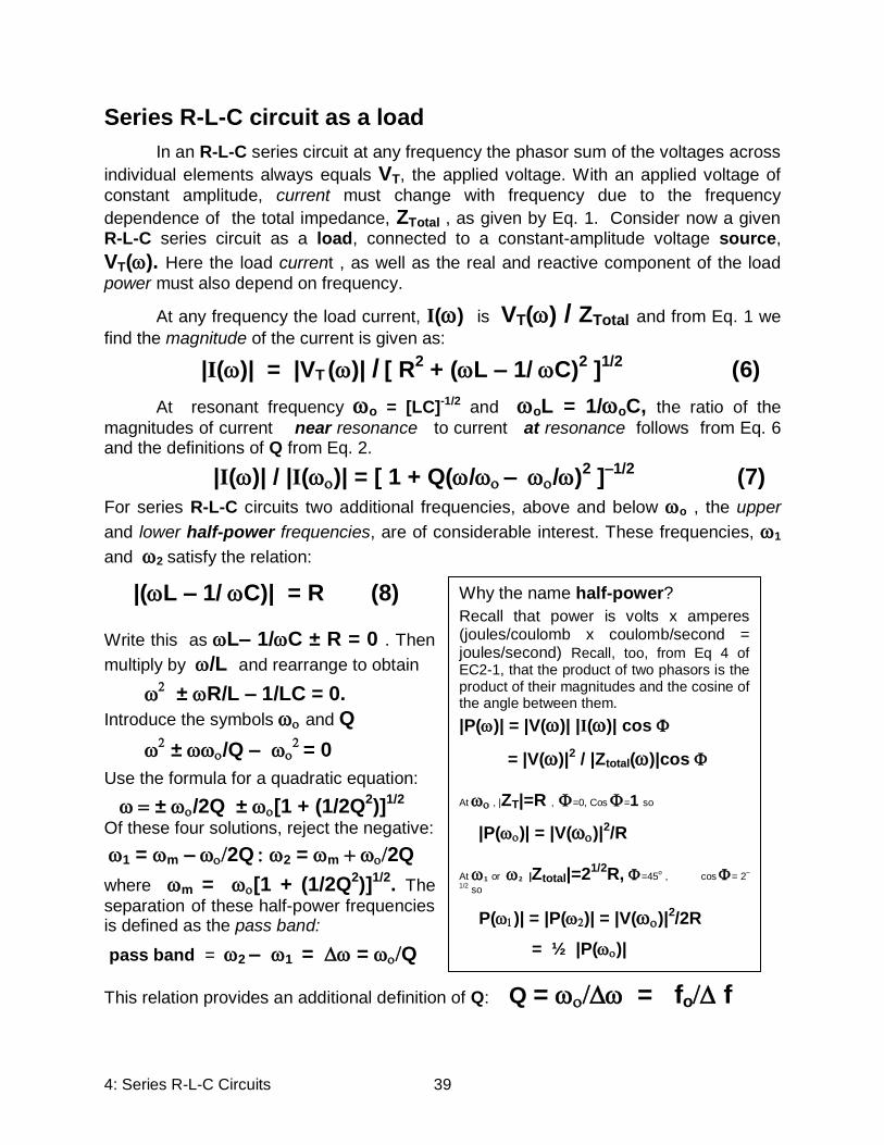
Why the name half-power?
Recall that power is volts x amperes (joules/coulomb x coulomb/second = joules/second) Recall, too, from Eq 4 of EC2-1, that the product of two phasors is the product of their magnitudes and the cosine of the angle between them.
|P()| = |V()| |I()| cos
= |V()|2 / |Ztotal()|cos
At , |ZT|=R , =0, Cos =1 so
|P()| = |V()|2/R
At 1 or 2 |Ztotal|=21/2R,=45o , cos= 2
–
1/2 so
P()| = |P()| = |V()|2/2R
= ½ |P()|
Series R-L-C circuit as a load
In an R-L-C series circuit at any frequency the phasor sum of the voltages across
individual elements always equals VT, the applied voltage. With an applied voltage of
constant amplitude, current must change with frequency due to the frequency
dependence of the total impedance, ZTotal , as given by Eq. 1. Consider now a given R-L-C series circuit as a load, connected to a constant-amplitude voltage source,
VT(). Here the load current , as well as the real and reactive component of the load
power must also depend on frequency.
At any frequency the load current, I() is VT() / ZTotal and from Eq. 1 we
find the magnitude of the current is given as:
|I()| = |VT ()| / [ R2 + (L – 1/C)
2 ]
1/2 (6)
At resonant frequency o = [LC]-1/2 and oL = 1/oC, the ratio of the
magnitudes of current near resonance to current at resonance follows from Eq. 6 and the definitions of Q from Eq. 2.
|I()| / |I()| = [ 1 + Q(/–/)2 ]
–1/2 (7)
For series R-L-C circuits two additional frequencies, above and below o , the upper
and lower half-power frequencies, are of considerable interest. These frequencies, 1
and 2 satisfy the relation:
|(L – 1/C)| = R (8)
Write this as L– 1/C ± R = 0 . Then
multiply by /L and rearrange to obtain
± R/L – 1/LC = 0.
Introduce the symbols and Q
± /Q –
= 0
Use the formula for a quadratic equation:
± /2Q ± [1 + (1/2Q2)]
1/2
Of these four solutions, reject the negative:
1 = m–2Q2 = m2Q
where m = [1 + (1/2Q2)]
1/2. The
separation of these half-power frequencies is defined as the pass band:
pass band = 2 – 1 = = Q
This relation provides an additional definition of Q: Q = = fo f
4: Series R-L-C Circuits 40
Q = Q m =[1 + (1 / 2Q)2]1/2
1.5 0.667 1.054
2 0.500 1.031
3 0.333 1.014
4 0.250 1.008
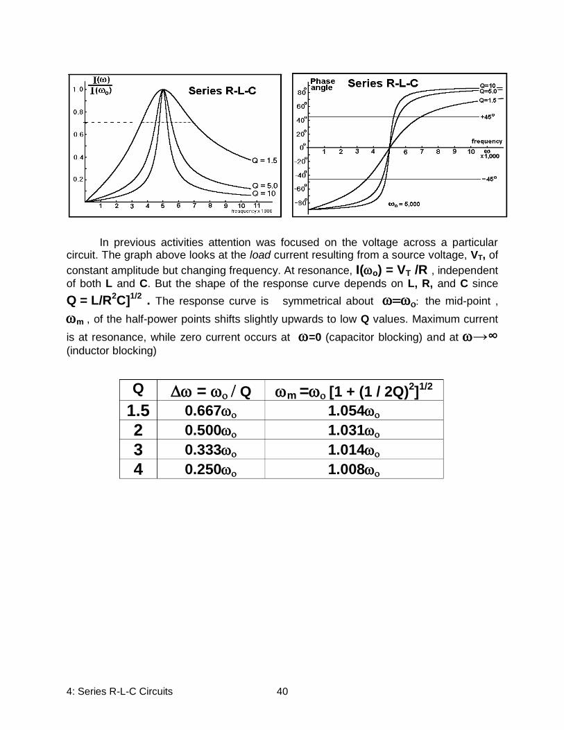
In previous activities attention was focused on the voltage across a particular circuit. The graph above looks at the load current resulting from a source voltage, VT, of
constant amplitude but changing frequency. At resonance, I(o) = VT /R , independent
of both L and C. But the shape of the response curve depends on L, R, and C since
Q = L/R2C]
1/2 . The response curve is symmetrical about the mid-point ,
m ,of the half-power points shifts slightly upwards to low Q values. Maximum current
is at resonance, while zero current occurs at =0 (capacitor blocking) and at →∞ (inductor blocking)

4: Series R-L-C Circuits 41
Activity 4-5 Pass band
High Q
1: Measure r. Set the signal source to f =1000 hz. Set the variable inductor close to maximum.
Set the decade resistor in series with the inductor to 0 Adjust C so that the circuit is in
resonance.
2: Adjust the signal amplitude so that VT has a large but easily-remembered value as 1.000 or 1.500 or greater. Measure VT, Vr and calculate R = r VT/ Vr . Also calculate Io = Vr / r, the current at resonance. Calculate I* = Io 2–1/2 = 0.707 Io
3: Reduce the signal frequency so that the phase meter indicates an approximate phase angle of 45o . Adjust the signal frequency and amplitude so that circuit current, given by Vr/r. equals I* while VT is maintained at its original value. Make these adjustments as carefully as possible. A slight change in voltage corresponds to a significant change in frequency. Record this value
as f1 (1=2f1)
4: Repeat step 3, but this time increase the frequency above 1000 hz
5: Calculate f = f2 – f1 and calculate the ratio fo / f . This is the Q of the circuit.
Compare this value of Q with 1/RoC . . Find the mid-point of f1 and f2 , (f1 + f2) / 2 and compare this with fo [1+ 1/Q2]1/2
Low Q
Recall that Q = [L/R2C] . To reduce Q but maintain the same resonant frequency, reduce L, increase R and C.
6: Reset the variable inductor close to its minimum value. Set the adjustable resistor in series
with the inductor to 150 . Set f = 1000 hz . Then adjust C so that the circuit is in resonance. Then proceed as in steps 2 to 5.

4: Series R-L-C Circuits 42
L mh Cnf [4C]
1/2 fo
80.0 800 629
80.0 500 796 80.0 200 1259
50.0 800 796 50.0 600 919
50.0 400 1126
L mh [4L]
1/2 Cnf
90.0 281
80.0 317
70.0 362
60.0 423
50.0 509
40.0 634
Data Sheet Experiment # EC2-4
Series R-L-C Circuits
Name ______________________________ Date__________
Activity 4-1: Verify the relation = [LC]–1/2
Given L and C, find fo Given L and fo=1000hz, find C
Activity 4-2 Inductor Resistance
L = 90.0 mH r = 50.0 coil _______
f hz Vr VT r(Vr/VT)
600
800
1000
1200
1400
1600
1800

4: Series R-L-C Circuits 43
Data Sheet Experiment # EC2-4, continued Activity 4-3 Series circuit “Quality” or Q
r = 50 , L = 90.0 mH, VT = 1.000 volts
f C nf Vr R VL L/R VC 1/RoC 500
1000 1500 2000
Activity 4-4 Close to resonance
First trial:
C = 999 nF f = 500 hz r ______ VT _______ Vr ________
R _______ Q ______ VT = 0.500 VC________ VC/ VT________
C’ = C Q2 /(Q2 + 1) _______ measured C’ _______ VC’ _________
VC’ / VT _________ [(Q2 + 1)/Q
2]1/2
_________ VC’ / VC ________
Arctan (1/Q) ________________ measured ____________ Second trial:
C = 999 nF f = 500 hz r ______ VT _______ Vr ________
Rtotal _______ Q ______ VT =1.000 VC_______ VC/ VT_______
C’ = C Q2 /(Q2 + 1) _______ measured C’ _______ VC’ _________
VC’ / VT _________ [(Q2 + 1)/Q
2]1/2
_________ VC’ / VC ________
Arctan (1/Q) ________________ measured ____________

4: Series R-L-C Circuits 44
Data Sheet Experiment # EC2-4, continued
Activity 4-5 Pass band
High Q
fo = 1000 hz
r _________ C __________ VT ________ Vr __________
R _________ Io __________ I* __________
f1 _________ f2 __________ f __________
Q = f / f ____________ Q = 1 / RC ____________
fm = (f1 + f2)/2 ________ fo [1+ (1/2Q)2]1/2
__________ Low Q
fo = 1000 hz
r __________ C __________ VT ________ Vr __________
R __________ Io ___________ I* __________
f1 _________ f2 __________ f __________
Q = f / f ____________ Q = 1 / RC ____________
fm = (f1 + f2)/2 ________ fo [1+ (1/2Q)2]1/2
__________

4: Series R-L-C Circuits 45
5: Parallel R-L-C Circuits 46
9xsw*8s20321vfr4*987xsw2
Parallel R-L-C Circuits ___________________________________________________________
Admittance
The equation for a straight line on an X-Y graph is normally written as y = mx
although x = (1/m)y also displays the same line. In the first form x is considered as
the independent variable, y the dependent variable. The dependent variable usually
stands along on the left side of the equation. Change the independent variable, and the dependent variable follows.
How about the complex form of Ohm’s law, V = IZ ? As written, V appears as the dependent variable: change the current and the voltage will also change. But often we think of the current as depending on the applied voltage and the properties of the
element. Current then becomes the dependent variable: I = V(1/Z) . Since this way of
looking at it has proven useful in certain applications, the (1/Z) expression is often
represented by the letter Y, and given the name admittance with the physical dimensions of reciprocal ohms. Often a special dimension name for admittance is used, the mho (ohm spelled backwards). Since impedance is a complex quantity, so its reciprocal, admittance, is also complex
By definition, admittance = 1 / impedance, Y = 1/Z. Therefore
Y = 1/Z = 1/ (R + jX) = (R - jX)/(R2 + X
2)
Two new terms are introduced, conductance, G, and susceptance, B:
Admittance is always the reciprocal of inductance. However conductance is the
reciprocal of resistance only if no reactance, X=0. Likewise susceptance is the
reciprocal of reactance only if no resistance, R=0. When dealing with inductors take
X = L , and with capacitors take X = –1/C
For elements in series the same current, T, passes through each; the total
voltage, VT, is the phasor sum of the voltages across each element:
VT = T (Z1 + Z2 + … + ZN) : Voltage = Current x (sum of impedance)
ELECTRIC CIRCUITS II EC2- 5
impedance = resistance + j reactance Z = R + jX (1)
admittance = conductance – j susceptance Y = G – jB
G = R/(R2 + X
2) B = X/(R
2 + X
2) (2)

5: Parallel R-L-C Circuits 47
For elements in parallel the same voltage, VT, appears across each; the total
current, T, is the phasor sum of the currents through each element:
IT = VT ( Y1 + Y2 + … + YN) Current = Voltage x (sum of admittance).
For elements in series, impedance concepts are generally more convenient; for elements in parallel , admittance concepts are often preferred
Parallel or Series
In an ideal inductor or capacitor (zero resistance) energy may be stored and later retrieved with no energy loss. Such ideal inductors are not readily available. In the previous discussion of series resonance, a real inductor was modeled as an ideal
inductor, LS , with a small series resistor, RS. An alternate and useful model is that of
an ideal inductor, LP , with a large parallel resistor, RP. The impedance of either model
should have the same magnitude and phase angle, that is, ZS = RS + j XS equals
ZP = RP jXP / (RP + jXP) . In the box
at right the denominator of ZP is first
rationalized. Since ZS = ZP their real
and imaginary parts are separately
equal. Likewise the phase angle, ,
for each model must be the same.
From this it follows that XS / RS = RP / XP .
Equation (2) of Experiment EC2-4 introduced the symbol Q as a quality factor for
a series resonant circuit (involving both L and C). Here the same symbol, Q, is
introduced as Q = XS / RS = RP / XP , in terms of L or C alone. With this notation the
results above may be expressed as:
For Q ≥ 10, notice that XP ≈ XS and RP ≈ Q
2 RS. For real capacitors, both
RP and RS are quite small, so the Q of a capacitor may be quite high, even a thousand
or more. For the two models mentioned above, a high Q means a quite small series
resistance and a quite large parallel resistance. Later it will be shown that Q is proportional to the ratio of maximum energy stored in the reactance to the energy dissipated by the resistance during one full cycle .
RS = RP / (1 + Q2) RP = RS (1 + Q
2) (3)
XS = XP 1/(1 + Q–2
) XP = XS (1 +Q–2
) (4)
5: Parallel R-L-C Circuits 48
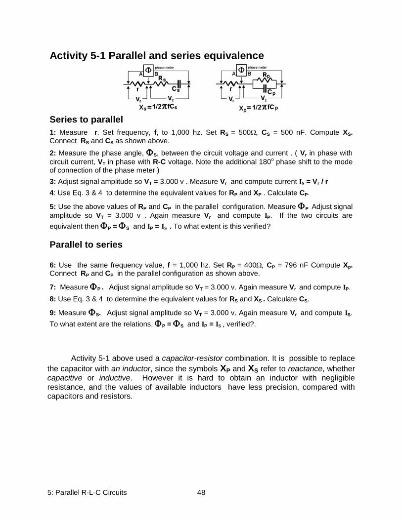
Activity 5-1 above used a capacitor-resistor combination. It is possible to replace
the capacitor with an inductor, since the symbols XP and XS refer to reactance, whether capacitive or inductive. However it is hard to obtain an inductor with negligible resistance, and the values of available inductors have less precision, compared with capacitors and resistors.
Activity 5-1 Parallel and series equivalence
Series to parallel
1: Measure r. Set frequency, f, to 1,000 hz. Set RS = 500 CS = 500 nF. Compute XS. Connect RS and CS as shown above. .
2: Measure the phase angle, S, between the circuit voltage and current . ( Vr in phase with
circuit current, VT in phase with R-C voltage. Note the additional 180o phase shift to the mode of connection of the phase meter )
3: Adjust signal amplitude so VT = 3.000 v . Measure Vr and compute current IS = Vr / r
4: Use Eq. 3 & 4 to determine the equivalent values for RP and XP . Calculate CP.
5: Use the above values of RP and CP in the parallel configuration. Measure P Adjust signal
amplitude so VT = 3.000 v . Again measure Vr and compute IP. If the two circuits are
equivalent then P = S and IP = IS . To what extent is this verified?
Parallel to series 6: Use the same frequency value, f = 1,000 hz. Set RP = 400 CP = 796 nF Compute Xp. Connect RP and CP in the parallel configuration as shown above.
7: Measure P . Adjust signal amplitude so VT = 3.000 v. Again measure Vr and compute IP.
8: Use Eq. 3 & 4 to determine the equivalent values for RS and XS . Calculate CS.
9: Measure S. Adjust signal amplitude so VT = 3.000 v. Again measure Vr and compute IS.
To what extent are the relations, P = S and IP = IS , verified?.
5: Parallel R-L-C Circuits 49
Parallel R-L-C
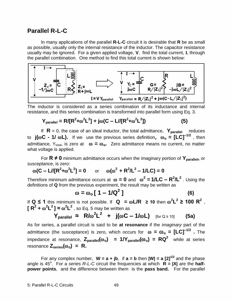
In many applications of the parallel R-L-C circuit it is desirable that R be as small as possible, usually only the internal resistance of the inductor. The capacitor resistance usually may be ignored. For a given applied voltage, V, find the total current, I, through the parallel combination. One method to find this total current is shown below:
The inductor is considered as a series combination of its inductance and internal resistance, and this series combination is transformed into parallel form using Eq. 3.
Yparallel = R/[R2+
2L
2] + j(C – L//[R
2+
2L
2]) (5)
If R = 0, the case of an ideal inductor, the total admittance, Yparallel reduces
to j(C - 1/ L). If we use the previous series definition, o = [LC]–1/2
, then
admittance, Ytotal, is zero at = o. Zero admittance means no current, no matter
what voltage is applied.
For R ≠ 0 minimum admittance occurs when the imaginary portion of Yparallel, or
susceptance, is zero:
(C – L//[R2+
2L
2] = 0 or (
2 + R
2/L
2 – 1/LC) = 0
Therefore minimum admittance occurs at = 0 and 2 =
1/LC – R
2/L
2 . Using the
definitions of Q from the previous experiment, the result may be written as
= o [ 1 – 1/Q2 ] (6)
If Q ≤ 1 this minimum is not possible. If Q = L/R ≥ 10 then 2L
2 ≥ 100 R
2 ,
[ R2 +
2L
2 ] ≈
2L
2 , so Eq. 5 may be written as
Yparallel ≈ R/2L
2 + j(C – 1/L) [for Q ≥ 10] (5a)
As for series, a parallel circuit is said to be at resonance if the imaginary part of the
admittance (the susceptance) is zero, which occurs for = o = [LC]–1/2
. The
impedance at resonance, Zparallel(o) = 1/Yparallel(o) = RQ2 while at series
resonance Zseries(o) = R.
For any complex number, W = a + jb, if a = b then |W| = a [2]1/2 and the phase angle is 45o. For a series R-L-C circuit the frequencies at which R = |X| are the half-power points, and the difference between them is the pass band. For the parallel

5: Parallel R-L-C Circuits 50
R-L-C circuit, at the frequencies where G = |B|, (C – 1/L) = ± R/2L
2 . Multiply
this by /C and re-arrange:
2– 1/LC = ± R/CL
2 or
2 ≈ o
2 ± o Q and ≈ o [ 1 ± 1/Q]
1/2 .
Apply the Taylor’s series approximation to this last form to obtain
≈ o [ 1 ± 1/Q]1/2
= o [ 1 ± ½ (1/Q) ± … ]
or 1 = o+ o 2Q , 2 = o– o/2Q, = 1– 2 = o/Q .
The pass bands for both serial and parallel R-L-C circuits are the same and
Q = o / = fo / f .
Activity 5-2 Parallel Resonance To obtain a higher Q for this activity use the air-core inductors from Experiment 12 of Electric Circuits I. In part A below we first use a series configuration to determine L, R and Q . For an air-core inductor the values of R should be only slightly greater that the DC resistance of the windings.
Part A
1: Set up the circuit as shown above. Set the function generator for f = 1,000 hz, sine wave, maximum amplitude. Adjust the variable capacitance, C, to bring the circuit into resonance
( = 180o ). Note that the phase meter reading is more stable if the values of VT and Vr
exceed one volt, so adjust the value of r accordingly. Compute R = r VT/Vr , L = [()2 C]–
1/2 and Q = 1/(f R C)
Part B
2: Set up the circuit as shown. Set f = 1000hz, r = 2000, and make any small adjustment
in C to bring the circuit into resonance. Measure VT and Vr . Compute I(fo) = Vr / r and
Z(fo) = VT / I .

5: Parallel R-L-C Circuits 51
Parallel R-L-C circuit with constant current source
The frequency-dependent impedance ( or admittance) of R-L-C circuits can sort out signals of differing frequencies. The low impedance at resonance of the series circuit easily accepts a particular signal while the high impedance ( low admittance ) of the parallel circuit can block the sane signal. From Ohm’s law, V = I Z , if the current, I(f), has a constant amplitude, the voltage, V(f), across the element increases with increasing impedance, Z. If Z is frequency dependent, then the amplitude of V(f) changes with frequency even though the amplitude of I(f) remains constant.
The collector current, Ic, of an NPN transistor in the common-emitter configuration is directly proportional to the
input base current, Ib, over a wide range of collector-emitter
voltage, Vce : Ic = Ib . If Ic passes through a load resistor,
Rload, an output voltage, Vload , appears:
Vload = Ic Rload = Ib Rload
Now if Rload, is replaced by a parallel R-L-C circuit, the gain
( ratio of Vload to Ib ) increases the closer the frequency of
Ib approaches the resonant frequency. Such a circuit is
found in most radios.
3: Increase the frequency above 1000 hz until the analog display of the phase meter reads
135o (corresponding to a 45o phase angle between VT and )
of frequency using the digital display of the phase meter where = (offset/period) x 360o.
Represent this frequency by f1 . Again measure Vr and VT and compute I(f1) and Z(f1)
4: Repeat step 3, but this time decreasing the frequency below 1000 hz to obtain f2 . Compute I(f2) and Z(f2).
5: Compute the pass band, f = f1 – f2 , and compare f0 / f with the Q value of step 1.
Compare Z(f1) and Z(f2) with Z(fo) [2]–1/2.
5: Parallel R-L-C Circuits 52
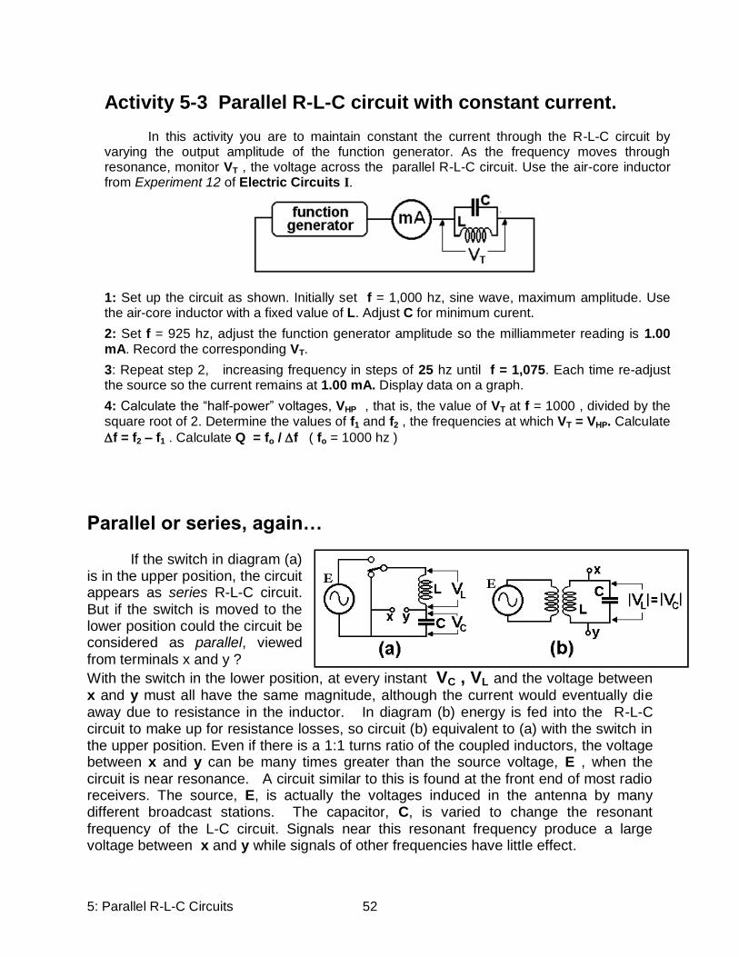
Parallel or series, again… If the switch in diagram (a) is in the upper position, the circuit appears as series R-L-C circuit. But if the switch is moved to the lower position could the circuit be considered as parallel, viewed from terminals x and y ?
With the switch in the lower position, at every instant VC , VL and the voltage between x and y must all have the same magnitude, although the current would eventually die away due to resistance in the inductor. In diagram (b) energy is fed into the R-L-C circuit to make up for resistance losses, so circuit (b) equivalent to (a) with the switch in the upper position. Even if there is a 1:1 turns ratio of the coupled inductors, the voltage between x and y can be many times greater than the source voltage, E , when the circuit is near resonance. A circuit similar to this is found at the front end of most radio receivers. The source, E, is actually the voltages induced in the antenna by many different broadcast stations. The capacitor, C, is varied to change the resonant frequency of the L-C circuit. Signals near this resonant frequency produce a large voltage between x and y while signals of other frequencies have little effect.
Activity 5-3 Parallel R-L-C circuit with constant current. In this activity you are to maintain constant the current through the R-L-C circuit by varying the output amplitude of the function generator. As the frequency moves through resonance, monitor VT , the voltage across the parallel R-L-C circuit. Use the air-core inductor from Experiment 12 of Electric Circuits I.
1: Set up the circuit as shown. Initially set f = 1,000 hz, sine wave, maximum amplitude. Use the air-core inductor with a fixed value of L. Adjust C for minimum curent.
2: Set f = 925 hz, adjust the function generator amplitude so the milliammeter reading is 1.00 mA. Record the corresponding VT.
3: Repeat step 2, increasing frequency in steps of 25 hz until f = 1,075. Each time re-adjust the source so the current remains at 1.00 mA. Display data on a graph.
4: Calculate the “half-power” voltages, VHP , that is, the value of VT at f = 1000 , divided by the square root of 2. Determine the values of f1 and f2 , the frequencies at which VT = VHP. Calculate
f = f2 – f1 . Calculate Q = fo / f ( fo = 1000 hz )
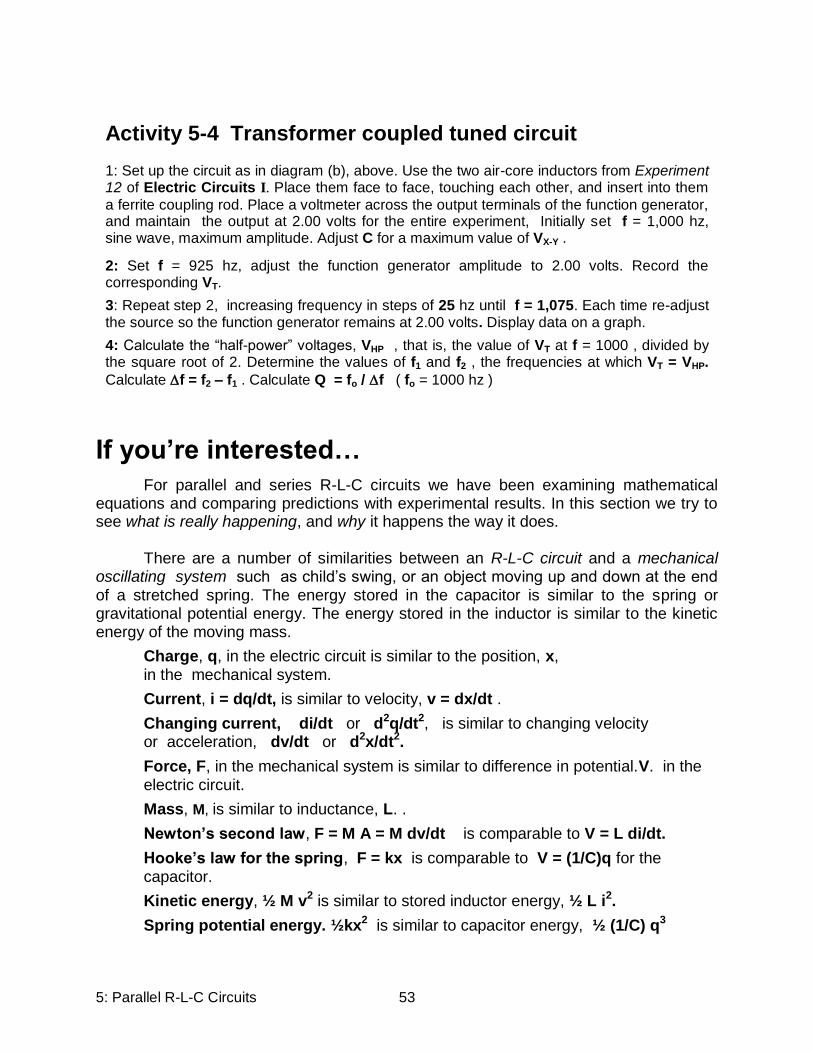
5: Parallel R-L-C Circuits 53
If you’re interested…
For parallel and series R-L-C circuits we have been examining mathematical equations and comparing predictions with experimental results. In this section we try to see what is really happening, and why it happens the way it does. There are a number of similarities between an R-L-C circuit and a mechanical oscillating system such as child’s swing, or an object moving up and down at the end of a stretched spring. The energy stored in the capacitor is similar to the spring or gravitational potential energy. The energy stored in the inductor is similar to the kinetic energy of the moving mass.
Charge, q, in the electric circuit is similar to the position, x, in the mechanical system.
Current, i = dq/dt, is similar to velocity, v = dx/dt .
Changing current, di/dt or d2q/dt2, is similar to changing velocity or acceleration, dv/dt or d2x/dt2.
Force, F, in the mechanical system is similar to difference in potential.V. in the electric circuit.
Mass, M, is similar to inductance, L. .
Newton’s second law, F = M A = M dv/dt is comparable to V = L di/dt.
Hooke’s law for the spring, F = kx is comparable to V = (1/C)q for the capacitor.
Kinetic energy, ½ M v2 is similar to stored inductor energy, ½ L i2.
Spring potential energy. ½kx2 is similar to capacitor energy, ½ (1/C) q3
Activity 5-4 Transformer coupled tuned circuit 1: Set up the circuit as in diagram (b), above. Use the two air-core inductors from Experiment 12 of Electric Circuits I. Place them face to face, touching each other, and insert into them
a ferrite coupling rod. Place a voltmeter across the output terminals of the function generator, and maintain the output at 2.00 volts for the entire experiment, Initially set f = 1,000 hz, sine wave, maximum amplitude. Adjust C for a maximum value of VX-Y .
2: Set f = 925 hz, adjust the function generator amplitude to 2.00 volts. Record the corresponding VT.
3: Repeat step 2, increasing frequency in steps of 25 hz until f = 1,075. Each time re-adjust the source so the function generator remains at 2.00 volts. Display data on a graph.
4: Calculate the “half-power” voltages, VHP , that is, the value of VT at f = 1000 , divided by the square root of 2. Determine the values of f1 and f2 , the frequencies at which VT = VHP.
Calculate f = f2 – f1 . Calculate Q = fo / f ( fo = 1000 hz )

5: Parallel R-L-C Circuits 54
Viscous friction, directly proportional to velocity, is comparable to electrical resistance, R, directly proportional to current..
The mechanical system’s natural frequency in simple harmonic motion is comparable to the electric system’s resonant frequency Stored energy is never negative . It is independent of the algebraic sign for
current and charge, or velocity and position). As an instantaneous quantity, enegy is independent of frequency or time. In R-L-C circuits energy may be passes back and forth between inductor and capacitor and also between the circuit and surrounding components. Recall that electrical energy is transferred whenever a potential difference exists across an element through which a current passes ; mechanical energy is transferred whenever a resultant force acts on an object in motion. If positive charge moves (current) from lower to higher potential (flashlight battery, generator or discharging capacitor), the element delivers energy to the circuit. If from higher to lower potential (resistor, motor, or charging capacitor) the element accepts energy . So also for a mechanical system: a resultant force in the direction of motion adds energy to the system; if opposite the direction of motion energy is subtracted.. A mechanical system without friction can remain in oscillation indefinitely. Natural frequency is determined by mass and the Hooke’s law constant. The maximum potential energy just equals the maximum kinetic energy and their sum at any instant is the total stored energy of the system. To increase or decrease this total energy mechanical work is done on or by the system only to change the system’s total energy. .
At resonance, with no resistance: = o , R = 0
Likewise an L-C circuit without resistance could remain in oscillation
indefinitely. Resonant frequency is determined by L and C; o = [LC]–1/2 . Total energy would remain constant. Maximum values of capacitor and inductor energy are equal Electrical work would be done on or by the system only to change this total energy.
If this idealized resistance-
less L-C circuit is series, current continually flows into and out of the system, but at resonance there is no potential difference ( zero impedance ), so no energy is transferred.

5: Parallel R-L-C Circuits 55
The voltage across any element is the product of current and impedance. Since the same current passes through the inductor and capacitor, and their reactance have
the same magnitude, but differ in phase by 180o, it follows that |VL| = |VC| and differ
in phase by just 180o , and so their phasor sum is VL + VC = VT = 0.
If parallel , a voltage appears across the terminals but no current enters or leaves ( zero admittance ). Since the inductor and capacitor are in parallel, the voltages across each must be equal. At resonance, by definition the reactance of each has the same
magnitude: |oL| = |1/ oC|, so the currents, IC and IL , have the same magnitude.
From Kirchoff’s current law, the algebraic sum of currents entering any node, such as x
or y in the diagram, must total zero. Therefore the currents labeled I? must also be
zero.
At resonance, with resistance: = o , R ≠ 0
If resistance, R, is present, usually inherent in the windings and core material of
the inductor, electrical energy is continuously converted into heat at the rate of I2R .
Therefore to maintain the total energy constant, additional electric energy must be
supplied. This requires a voltage drop, Vtotal , across the series circuit and a current,
Itotal, through the parallel circuit. Power-in equals power-out, or Vtotal Itotal = I2R.
The impedance, Z, of any element is defined as Vtotal / Itotal. For the series
circuit all current passes through the resistance, Itotal = I, so
This is not the case for the parallel R-L-C circuit, for the circulating current through the
capacitor and inductor is not the same as the total current through the circuit: I ≠ Itotal.
The total voltage equals the voltage across the capacitor, |Vtotal| = |I/oC|, so from
the energy relation:
Vtotal Itotal . = (I/oC) Itotal = I2R or I = Itotal (1/RoC) = ItotalQ
Zseries = Vtotal / Itotal = R.
Zparalel = Vtotal / Itotal = Q2 R
5: Parallel R-L-C Circuits 56
Even though the same physical inductor with internal resistance, R, is used, the impedance of the parallel and series R-L-C circuits are quite different
Off resonance: ≠ o
In the series R-L-C circuit, the same current, Itotal , flows through the inductor
and capacitor but when off resonance their reactance is no longer equal since L ≠
1/C . Therefore VL ≠ VC . The combination then behaves as a single element,
inductor or capacitor, depending on which reactance has the greater magnitude.
In the parallel R-L-C circuit, the same voltage, Vtotal , always appears across
the inductor and capacitor. Since their reactance is not the same, |IC| no longer equals |IL| and Kirchoff’s law no longer requires that I? or Itotal be zero. The additional current
flows through the branch with the lesser impedance. The combination then behaves as a single element, inductor or capacitor, depending on which reactance has the lesser magnitude.
Resistance and Resonant Frequency Resonant frequency for the R-L-C circuit is independent of frequency and
amplitude (assuming the R, L and C values do not change), just as the resonant frequency of a mechanical system in simple harmonic motion is independent of frequency and amplitude (assuming that the mass and the force and friction constants do not change). But why does resistance or friction change the natural resonant frequency?
In a mechanical system. such as a swinging pendulum, at the end-points where speed is zero just for a moment, all the stored energy is potential, at the midpoint it is all kinetic. The time to move between end- points is one half the period. Now a friction force proportional to speed slows down the moving object, causing it to take longer to move between end-points, causing a longer period and a lower frequency.
In an electrical system the fully charge capacitor, either positive or negative, corresponds to the end-points; the midpoint is the moment of maximum current through the inductor. The time between the capacitor being fully charged, either positive or negative, is one half the period If resistance, R, is present, which is proportional to
current, I ( = dq/dt, the rate of change of charge) , it will take slightly longer for the capacitor to charge and discharge, since current is less. Therefore the period is greater and the frequency less.
Storing Energy
A very gentle push on a child’s swing, done with the proper timing, can cause the swing to fly high and wide. The timing depends on the natural frequency of the swing.
5: Parallel R-L-C Circuits 57
Each gentle push increases little by little the total energy of the system, until the rate of energy loss due to friction just balances to rate of energy supplied by the gentle pushes.
A similar situation holds for a parallel R-L-C circuit. A very small voltage at the right frequency coupled through transformer action to the inductor can produce a dramatic increase in the circulating current and stored energy. The increase continues until the rate of energy loss due to resistance, R, just balances the rate of energy input through the transformer action.
The greater the circulating current, Imax sin ot, the greater the total stored
energy ( ½ Imax2 L) . The energy lost during one cycle due to resistance can be found
by integrating the quantity I2R ( = Imax
2 R sin2 ot ) from t = 0 to t = T. Use the relation
sin2 = ½ [1 - cos 2] . The ratio of these two energy values is found as
The greater the Q, the smaller the fraction of energy lost each cycle, and the
longer the time for the circulating current to decrease to, say, 1% of its initial value.
Recall that Q is also a measure of the pass band, Q = fo / f . The higher the Q, the
“sharper” is the resonance. The impedance of a parallel R-L-C circuit at resonance is
given by Zparallel(o) = R Q2.
For the series configuration, Vcapacitor / Vtotal = [1 + Q
2]1/2
. Q is aptly called the quality of a resonant circuit.
(stored energy) / (energy loss each cycle) = oL / 2R = Q / 2

5: Parallel R-L-C Circuits 58
Data Sheet Experiment # EC2-5
Parallel R-L-C Circuits
Name ______________________________ Date__________
Activity 5-1: Parallel and series equivalence
f = 1,000 VT = 3.000 v
Series to parallel
RS = 500 CS = 500 nF XS _________
Vr __________ S ____________ IS ____________
computed: RP ________ XP__________ CP_________
Vr __________P ____________ IP ____________ Parallel to series
Rp = 400 CP = 796 nF XP _________
Vr __________ P ____________ IP ____________
computed: RS ________ XS__________ CS_________
Vr __________S ____________ IS ____________ Activity 5-2 Parallel Resonance Part A
VT _________ Vr _________ r _______ C _________
R _________ L _________ Q __________
Part B r = 2000
fo = 1000 VT ______ Vr _______ I(fo) ________ Z(fo) ________
f1 ______ VT ______ Vr _______ I(f1) ________ Z(f2) ________
f2 _____ VT ______ Vr _______ I(f2) ________ Z(f2) ________
f______ fo/f ________ Z(fo)[2]–1/2__________
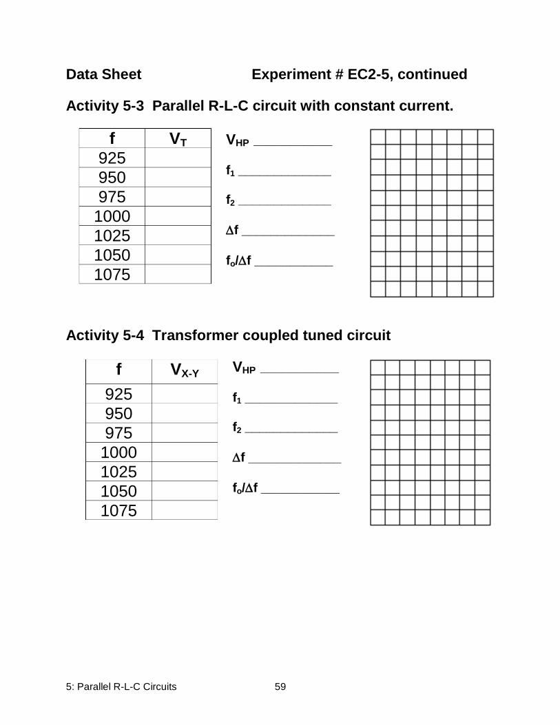
5: Parallel R-L-C Circuits 59
f VT
925
950
975
1000
1025
1050
1075
f VX-Y
925
950
975
1000
1025
1050
1075
Data Sheet Experiment # EC2-5, continued
Activity 5-3 Parallel R-L-C circuit with constant current. VHP ___________ f1 _____________ f2 _____________
f _____________
fo/f ___________
Activity 5-4 Transformer coupled tuned circuit
VHP ___________ f1 _____________ f2 _____________
f _____________
fo/f ___________

5: Parallel R-L-C Circuits 60
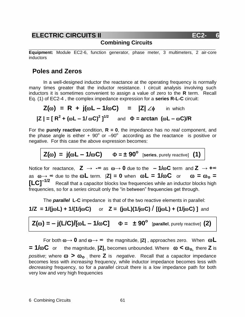
6 Combining Circuits 61
Combining Circuits _____________________________________________________________________________________________ Equipment: Module EC2-6, function generator, phase meter, 3 multimeters, 2 air-core
inductors
Poles and Zeros
In a well-designed inductor the reactance at the operating frequency is normally many times greater that the inductor resistance. I circuit analysis involving such inductors it is sometimes convenient to assign a value of zero to the R term. Recall Eq. (1) of EC2-4 , the complex impedance expression for a series R-L-C circuit:
Z() = R + j(L – 1/C) = |Z| in which
|Z | = [ R2 + (L – 1/C)
2 ]
1/2 and = arctan (L – C)/R
For the purely reactive condition, R = 0, the impedance has no real component, and the phase angle is either + 90o or –90o according as the reactance is positive or negative. For this case the above expression becomes:
Notice for reactance, Z → -∞ as → 0 due to the – 1/C term and Z → +∞
as → ∞ due to the L term. |Z| = 0 when L = 1/C or = o = [LC]
–1/2 Recall that a capacitor blocks low frequencies while an inductor blocks high
frequencies, so for a series circuit only the “in between” frequencies get through.
The parallel L-C impedance is that of the two reactive elements in parallel:
1/Z = 1/(jL) + 1/(1/jC) or Z = (jL)(1/jC) / [(jL) + (1/jC) ] and
For both → 0 and → ∞ the magnitude, |Z| , approaches zero. When L
= 1/C or the magnitude, |Z|, becomes unbounded. Where < o, there Z is
positive; where > o , there Z is negative. Recall that a capacitor impedance
becomes less with increasing frequency, while inductor impedance becomes less with decreasing frequency, so for a parallel circuit there is a low impedance path for both very low and very high frequencies
ELECTRIC CIRCUITS II EC2- 6 656
Z() = j(L – 1/C) = ± 90o
[series, purely reactive] (1)
Z() = – j(L/C)/[L – 1/C] = ± 90o
[parallel, purely reactive] (2)
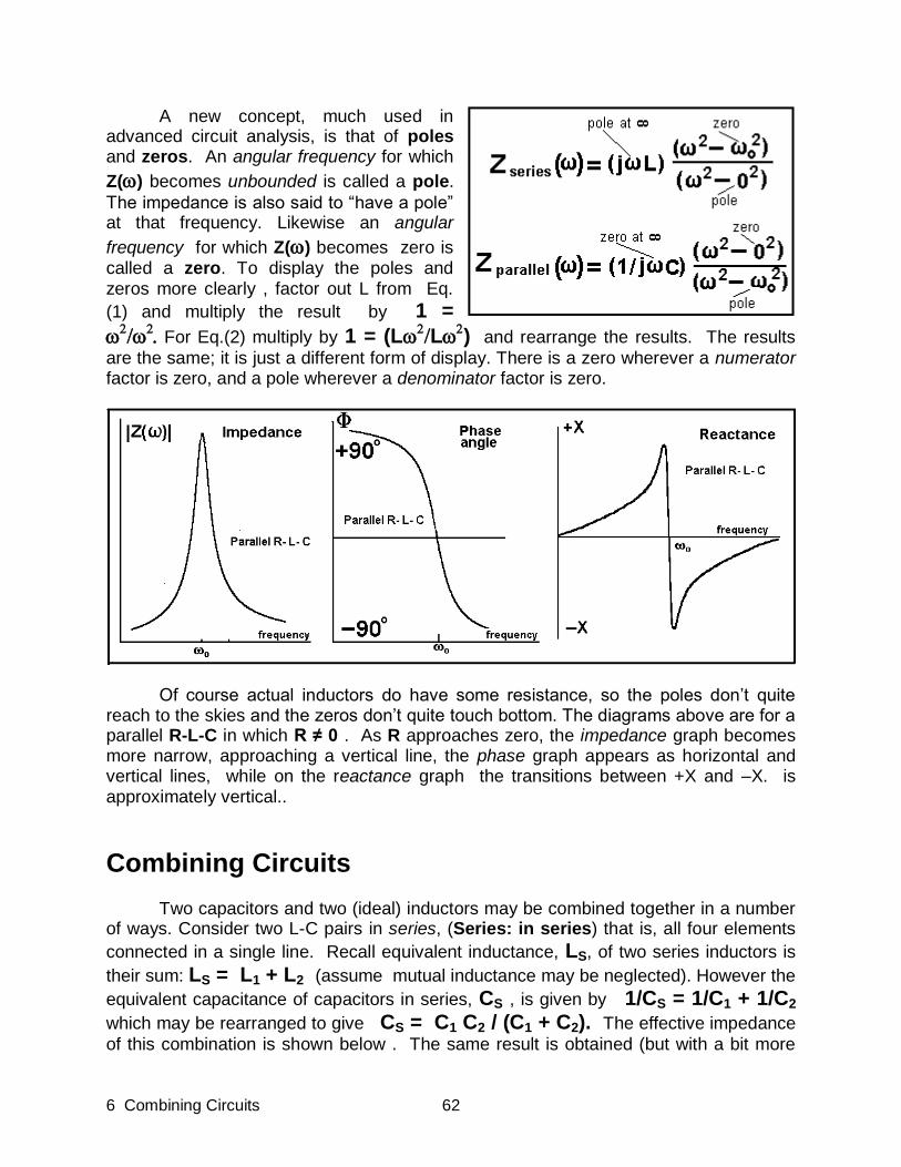
6 Combining Circuits 62
A new concept, much used in advanced circuit analysis, is that of poles and zeros. An angular frequency for which
Z() becomes unbounded is called a pole.
The impedance is also said to “have a pole” at that frequency. Likewise an angular
frequency for which Z() becomes zero is called a zero. To display the poles and zeros more clearly , factor out L from Eq.
(1) and multiply the result by 1 =
For Eq.(2) multiply by 1 = (L
L
) and rearrange the results. The results
are the same; it is just a different form of display. There is a zero wherever a numerator factor is zero, and a pole wherever a denominator factor is zero.
Of course actual inductors do have some resistance, so the poles don’t quite reach to the skies and the zeros don’t quite touch bottom. The diagrams above are for a parallel R-L-C in which R ≠ 0 . As R approaches zero, the impedance graph becomes more narrow, approaching a vertical line, the phase graph appears as horizontal and vertical lines, while on the reactance graph the transitions between +X and –X. is approximately vertical..
Combining Circuits Two capacitors and two (ideal) inductors may be combined together in a number of ways. Consider two L-C pairs in series, (Series: in series) that is, all four elements
connected in a single line. Recall equivalent inductance, LS, of two series inductors is
their sum: LS = L1 + L2 (assume mutual inductance may be neglected). However the
equivalent capacitance of capacitors in series, CS , is given by 1/CS = 1/C1 + 1/C2 which may be rearranged to give CS = C1 C2 / (C1 + C2). The effective impedance
of this combination is shown below . The same result is obtained (but with a bit more
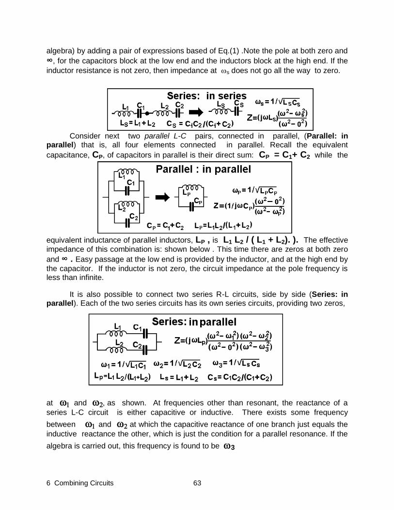
6 Combining Circuits 63
algebra) by adding a pair of expressions based of Eq.(1) .Note the pole at both zero and
∞, for the capacitors block at the low end and the inductors block at the high end. If the
inductor resistance is not zero, then impedance at s does not go all the way to zero.
Consider next two parallel L-C pairs, connected in parallel, (Parallel: in parallel) that is, all four elements connected in parallel. Recall the equivalent
capacitance, CP, of capacitors in parallel is their direct sum: CP = C1+ C2 while the
equivalent inductance of parallel inductors, LP , is L1 L2 / ( L1 + L2). ). The effective
impedance of this combination is: shown below . This time there are zeros at both zero
and ∞ . Easy passage at the low end is provided by the inductor, and at the high end by
the capacitor. If the inductor is not zero, the circuit impedance at the pole frequency is less than infinite.
It is also possible to connect two series R-L circuits, side by side (Series: in parallel). Each of the two series circuits has its own series circuits, providing two zeros,
at andas shown. At frequencies other than resonant, the reactance of a
series L-C circuit is either capacitive or inductive. There exists some frequency
between andat which the capacitive reactance of one branch just equals the
inductive reactance the other, which is just the condition for a parallel resonance. If the
algebra is carried out, this frequency is found to be 3
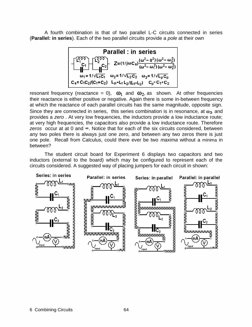
6 Combining Circuits 64
A fourth combination is that of two parallel L-C circuits connected in series (Parallel: in series). Each of the two parallel circuits provide a pole at their own
resonant frequency (reactance = 0), andas shown. At other frequencies
their reactance is either positive or negative. Again there is some in-between frequency at which the reactance of each parallel circuits has the same magnitude, opposite sign.
Since they are connected in series, this series combination is in resonance, at 3. and provides a zero . At very low frequencies, the inductors provide a low inductance route; at very high frequencies, the capacitors also provide a low inductance route. Therefore zeros occur at at 0 and ∞. Notice that for each of the six circuits considered, between any two poles there is always just one zero, and between any two zeros there is just one pole. Recall from Calculus, could there ever be two maxima without a minima in between?
The student circuit board for Experiment 6 displays two capacitors and two inductors (external to the board) which may be configured to represent each of the circuits considered. A suggested way of placing jumpers for each circuit in shown:
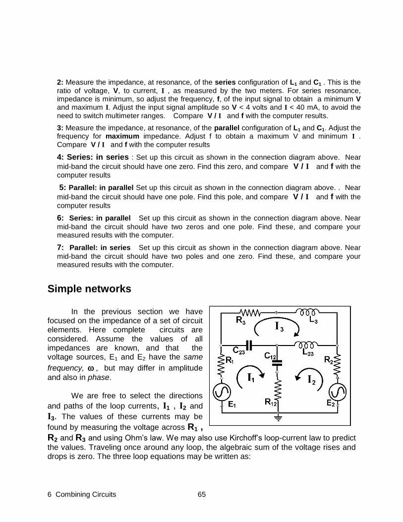
6 Combining Circuits 65
Simple networks In the previous section we have focused on the impedance of a set of circuit elements. Here complete circuits are considered. Assume the values of all impedances are known, and that the voltage sources, E1 and E2 have the same
frequency, but may differ in amplitude
and also in phase. We are free to select the directions
and paths of the loop currents, I1 , I2 and I3. The values of these currents may be
found by measuring the voltage across R1 , R2 and R3 and using Ohm’s law. We may also use Kirchoff’s loop-current law to predict
the values. Traveling once around any loop, the algebraic sum of the voltage rises and drops is zero. The three loop equations may be written as:
2: Measure the impedance, at resonance, of the series configuration of L1 and C1 . This is the ratio of voltage, V, to current, I , as measured by the two meters. For series resonance, impedance is minimum, so adjust the frequency, f, of the input signal to obtain a minimum V and maximum I. Adjust the input signal amplitude so V < 4 volts and I < 40 mA, to avoid the need to switch multimeter ranges. Compare V / I and f with the computer results.
3: Measure the impedance, at resonance, of the parallel configuration of L1 and C1. Adjust the frequency for maximum impedance. Adjust f to obtain a maximum V and minimum I . Compare V / I and f with the computer results
4: Series: in series : Set up this circuit as shown in the connection diagram above. Near
mid-band the circuit should have one zero. Find this zero, and compare V / I and f with the
computer results
5: Parallel: in parallel Set up this circuit as shown in the connection diagram above. . Near
mid-band the circuit should have one pole. Find this pole, and compare V / I and f with the
computer results
6: Series: in parallel Set up this circuit as shown in the connection diagram above. Near
mid-band the circuit should have two zeros and one pole. Find these, and compare your measured results with the computer.
7: Parallel: in series Set up this circuit as shown in the connection diagram above. Near
mid-band the circuit should have two poles and one zero. Find these, and compare your measured results with the computer.
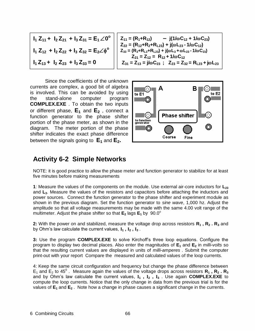
6 Combining Circuits 66
I1 Z11 + I2 Z21 + I3 Z31 = E1 0o
I1 Z12 + I2 Z22 + I3 Z32 = E2o
I1 Z13 + I2 Z23 + I3 Z33 = 0
Z11 = (R1+R12) – j(1/C12 + 1/C23)
Z22 = (R12+R2+RL23) + j(L23 - 1/C12) Z33 = (R3+RL3+RL23) + j(L3 + L23 - 1/C23)
Z21 = Z12 = R12 + 1/C12
Z31 = Z13 = j/C23 ; Z23 = Z32 = RL23 + jL23
Since the coefficients of the unknown currents are complex, a good bit of algebra is involved. This can be avoided by using the stand-alone computer program COMPLEX.EXE . To obtain the two inputs
or different phase, E1 and E2 , connect a
function generator to the phase shifter portion of the phase meter, as shown in the diagram. The meter portion of the phase shifter indicates the exact phase difference
between the signals going to E1 and E2.
Activity 6-2 Simple Networks NOTE: it is good practice to allow the phase meter and function generator to stabilize for at least five minutes before making measurements 1: Measure the values of the components on the module. Use external air-core inductors for L23 and L3. Measure the values of the resistors and capacitors before attaching the inductors and power sources. Connect the function generator to the phase shifter and experiment module as shown in the previous diagram. Set the function generator to sine wave, 1,000 hz. Adjust the amplitude so that all voltage measurements may be made with the same 4.00 volt range of the multimeter. Adjust the phase shifter so that E2 lags E1 by 90.0o 2: With the power on and stabilized, measure the voltage drop across resistors R1 , R2 . R3 and by Ohm’s law calculate the current values, I1 , I2 , I3 . 3: Use the program COMPLEX.EXE to solve Kirchoff’s three loop equations. Configure the program to display two decimal places. Also enter the magnitudes of E1 and E2 in milli-volts so that the resulting current values are displayed in units of milli-amperes . Submit the computer print-out with your report Compare the measured and calculated values of the loop currents. 4: Keep the same circuit configuration and frequency but change the phase difference between E1 and E2 to 450 . Measure again the values of the voltage drops across resistors R1 , R2 . R3 and by Ohm’s law calculate the current values, I1 , I2 , I3 . Use again COMPLEX.EXE to
compute the loop currents. Notice that the only change in data from the previous trial is for the values of E1 and E2 . Note how a change in phase causes a significant change in the currents.

6 Combining Circuits 67
Reciprocity theorem
The reciprocity theorem states:
If a source of emf, E, located at one point in a network
composed of bilateral circuit elements, produces a current, I,
at a second point in the network, the same source of emf, E,
acting at the second point will produce the same current, I, at the first point. Kerchner & Corcoron, AC Circuits 4
th Ed., pg 196
Recall that diodes and transistors are not bilateral elements, for their current-
voltage relation depends on the direction of the applied voltage. In the diagram above the ammeters are assumed to be ideal, that is, zero internal impedance. Notice that the
theorem says nothing about the input currents, Iin and Iin’ ; these depend on the input
impedances Z12 and Z34 which need not be equal.
Activity 6-3 Reciprocity theorem
Use the same network as in 6-2 above. Since zero-impedance ammeters are not readily available, determine the output currents by measuring VR2 and VR1, the voltage drops across the known resistors R1 and R2 and apply Ohm’s law.
1: Place a jumper across the terminals marked E2 .Connect the signal source (sine wave, 1,000 hz) across the E1 terminals as adjust amplitude to 3.500 volts. Measure VR2 and determine I3 , the output current.
2: Move the jumper from E2 to E1 . Place the source at E2 and re-adjust the amplitude to 3.500 volts. Measure VR1 and determine I1 , the output current. According to the reciprocity theorem
I1 should equal I3 .
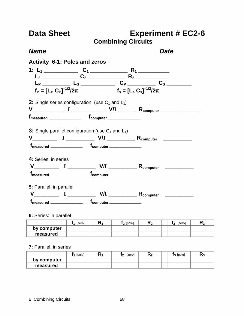
6 Combining Circuits 68
Data Sheet Experiment # EC2-6
Combining Circuits
Name ______________________________ Date__________
Activity 6-1: Poles and zeros
1: L1 ___________ C1 ____________ R1 __________ L2 ___________ C2 ____________ R2 __________ LP _________ LS ___________ CP _________ CS ________
fP = [LP CP]–1/2
/2 ___________ fs = [Ls Cs]–1/2
/2 ___________ 2: Single series configuration (use C1 and L1)
V_________ I __________ V/I _____ Rcomputer ___________ fmeasured _________ fcomputer _________ 3: Single parallel configuration (use C1 and L1)
V_______ I ________ V/I ________ Rcomputer ________ fmeasured _________ fcomputer _________ 4: Series: in series V_______ I ________ V/I ________ Rcomputer ________ fmeasured _________ fcomputer _________ 5: Parallel: in parallel
V_______ I ________ V/I ________ Rcomputer ________ fmeasured _________ fcomputer _________
6: Series: in parallel
f1 [zero] R1 f2 [pole] R2 f3 [zero] R3
by computer
measured
7: Parallel: in series
f1 [pole] R1 f2 [zero] R2 f3 [pole] R3
by computer
measured
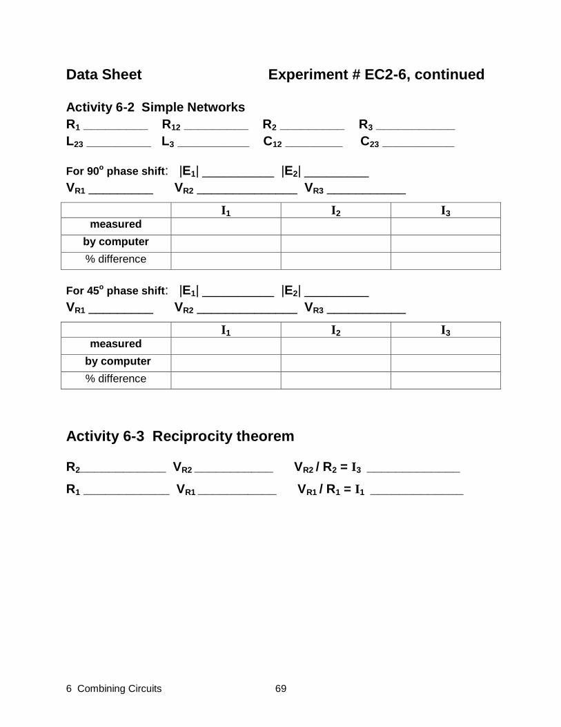
6 Combining Circuits 69
Data Sheet Experiment # EC2-6, continued Activity 6-2 Simple Networks
R1 _________ R12 _________ R2 _________ R3 ___________
L23 _________ L3 __________ C12 ________ C23 __________ For 90o phase shift: |E1| __________ |E2| _________
VR1 _________ VR2 ______________ VR3 ___________
I1 I2 I3 measured
by computer % difference
For 45o phase shift: |E1| __________ |E2| _________
VR1 _________ VR2 ______________ VR3 ___________
I1 I2 I3 measured
by computer % difference
Activity 6-3 Reciprocity theorem
R2____________ VR2 ___________ VR2 / R2 = I3 _____________
R1 ____________ VR1 ___________ VR1 / R1 = I1 _____________
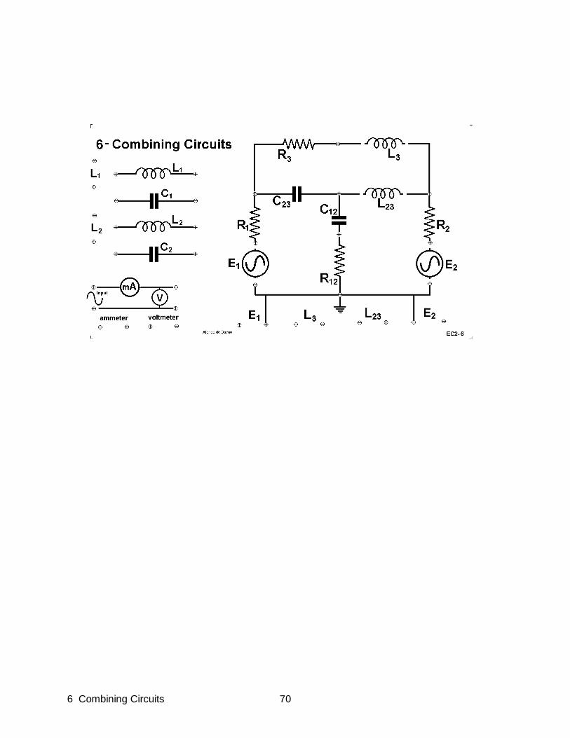
6 Combining Circuits 70
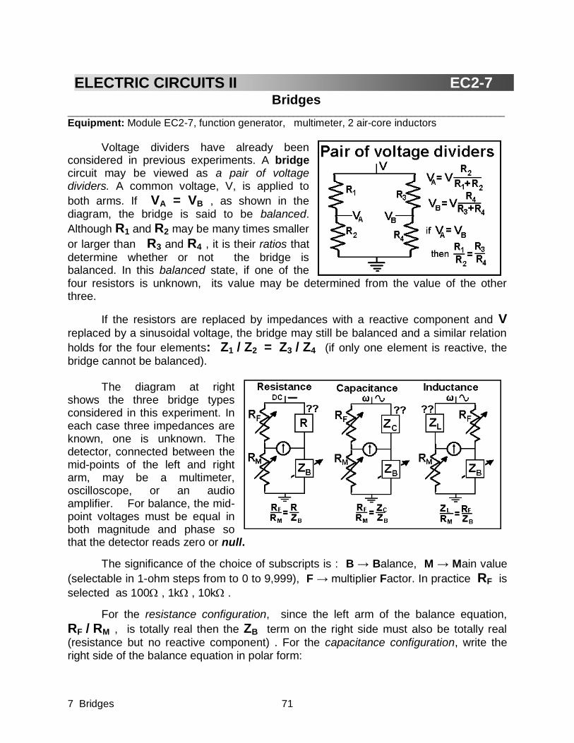
7 Bridges 71
Bridges _____________________________________________________________________________________________ Equipment: Module EC2-7, function generator, multimeter, 2 air-core inductors
Voltage dividers have already been considered in previous experiments. A bridge circuit may be viewed as a pair of voltage dividers. A common voltage, V, is applied to
both arms. If VA = VB , as shown in the diagram, the bridge is said to be balanced.
Although R1 and R2 may be many times smaller
or larger than R3 and R4 , it is their ratios that
determine whether or not the bridge is balanced. In this balanced state, if one of the four resistors is unknown, its value may be determined from the value of the other three.
If the resistors are replaced by impedances with a reactive component and V
replaced by a sinusoidal voltage, the bridge may still be balanced and a similar relation
holds for the four elements: Z1 / Z2 = Z3 / Z4 (if only one element is reactive, the
bridge cannot be balanced).
The diagram at right shows the three bridge types considered in this experiment. In each case three impedances are known, one is unknown. The detector, connected between the mid-points of the left and right arm, may be a multimeter, oscilloscope, or an audio amplifier. For balance, the mid-point voltages must be equal in both magnitude and phase so that the detector reads zero or null.
The significance of the choice of subscripts is : B → Balance, M → Main value
(selectable in 1-ohm steps from to 0 to 9,999), F → multiplier Factor. In practice RF is
selected as 100 , 1k , 10k . For the resistance configuration, since the left arm of the balance equation,
RF / RM , is totally real then the ZB term on the right side must also be totally real
(resistance but no reactive component) . For the capacitance configuration, write the right side of the balance equation in polar form:
ELECTRIC CIRCUITS II EC2-7 656

7 Bridges 72
|ZC|C / |ZB|B = [|ZC|/|ZB|] C –B)
If C –B = 0 the right arm of the bridge is also real, a necessary condition for
bridge balance . For the inductive configuration, cross-multiply its balance equation:
RF RM = ZB ZL = |ZB| |ZL| B +L)
For balance B andL must have opposite sign and sum to zero. Since ZL is
inductive then ZB must be capacitive.
Although the bridge can measure resistance inductance and capacitance, ZB
never has to be inductive. The ZB portion of the bridge of this module may be switched
to give three different configurations; RB alone, or RB either in parallel or in series with
CB. RB is continuously variable between 0 and 25 k However for measuring an
unknown resistance, the variable RB is replaced by one of four fixed resistors. CB is
switch selectable as either 100.0 nf (1.000 x 10⁻⁷ farad) or 10.00 nf (1.000 x 10⁻⁸ farad).
The bridge used is shown. Connections under the board allow attaching power and the detector at side terminals to avoid congestion. A
decade resistor, 0–9999 is
connected at the RM terminals and an
ohmmeter at RB. To measure an
unknown inductor, attach it at L?? and connect the lower end of the
selected RF resistor to point B.
Unknown resistors or capacitors are
to be connected at C?? R?? and the
lower end of the selected RF resistor
connected to point A. Details of ZB are shown.
The value of RB is adjusted with the
Coarse and Fine controls. The Measure RB –Operate switch in the upper position isolates
the resistor from the circuit and connects it
directly to the terminals labeled RB at the
bottom edge of the module, to which an
ohmmeter may be attached. The Parallel–Series switch connects RB and CB either in
parallel or series . The next switch selects two different values for RC .The terminals of
the selected RC are exposed.
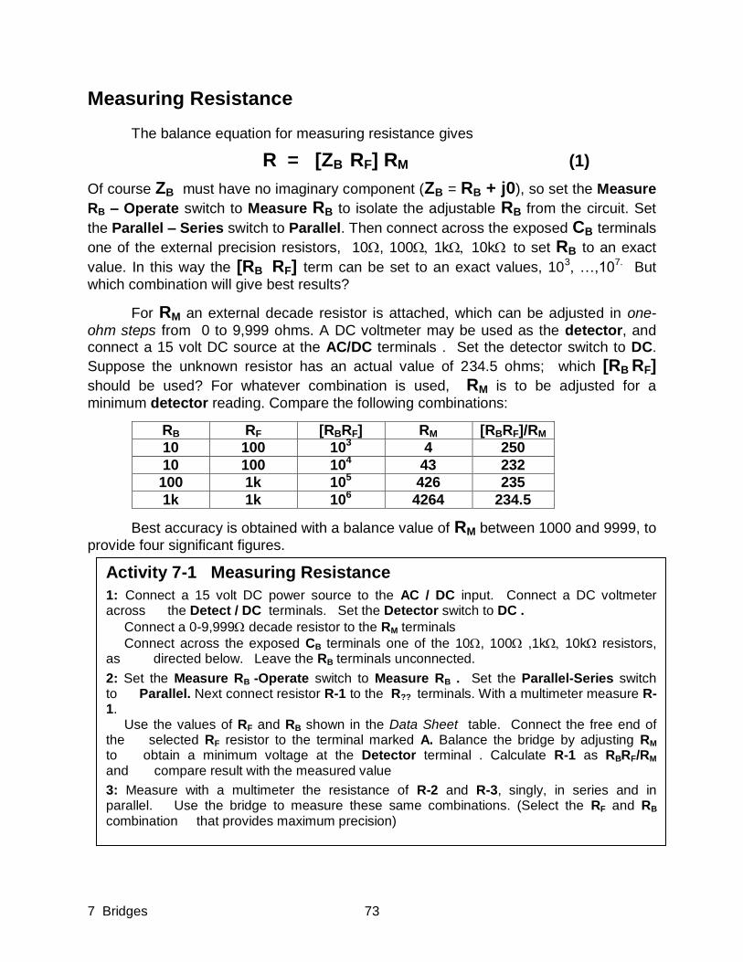
7 Bridges 73
Measuring Resistance
The balance equation for measuring resistance gives
R = [ZB RF] RM (1)
Of course ZB must have no imaginary component (ZB = RB + j0), so set the Measure
RB – Operate switch to Measure RB to isolate the adjustable RB from the circuit. Set
the Parallel – Series switch to Parallel. Then connect across the exposed CB terminals
one of the external precision resistors, 10, 100 1k10kto set RB to an exact
value. In this way the [RB RF] term can be set to an exact values, 103, …,107. But
which combination will give best results?
For RM an external decade resistor is attached, which can be adjusted in one-
ohm steps from 0 to 9,999 ohms. A DC voltmeter may be used as the detector, and connect a 15 volt DC source at the AC/DC terminals . Set the detector switch to DC.
Suppose the unknown resistor has an actual value of 234.5 ohms; which [RB RF] should be used? For whatever combination is used, RM is to be adjusted for a
minimum detector reading. Compare the following combinations:
RB RF [RBRF] RM [RBRF]/RM
10 100 103
4 250
10 100 104 43 232
100 1k 105 426 235
1k 1k 106 4264 234.5
Best accuracy is obtained with a balance value of RM between 1000 and 9999, to
provide four significant figures.
Activity 7-1 Measuring Resistance
1: Connect a 15 volt DC power source to the AC / DC input. Connect a DC voltmeter across the Detect / DC terminals. Set the Detector switch to DC .
Connect a 0-9,999 decade resistor to the RM terminals
Connect across the exposed CB terminals one of the 10, 100 ,1k 10k resistors, as directed below. Leave the RB terminals unconnected.
2: Set the Measure RB -Operate switch to Measure RB . Set the Parallel-Series switch to Parallel. Next connect resistor R-1 to the R??
terminals. With a multimeter measure R-1. Use the values of RF and RB shown in the Data Sheet table. Connect the free end of the selected RF resistor to the terminal marked A. Balance the bridge by adjusting RM to obtain a minimum voltage at the Detector terminal . Calculate R-1 as RBRF/RM and compare result with the measured value
3: Measure with a multimeter the resistance of R-2 and R-3, singly, in series and in parallel. Use the bridge to measure these same combinations. (Select the RF and RB combination that provides maximum precision)
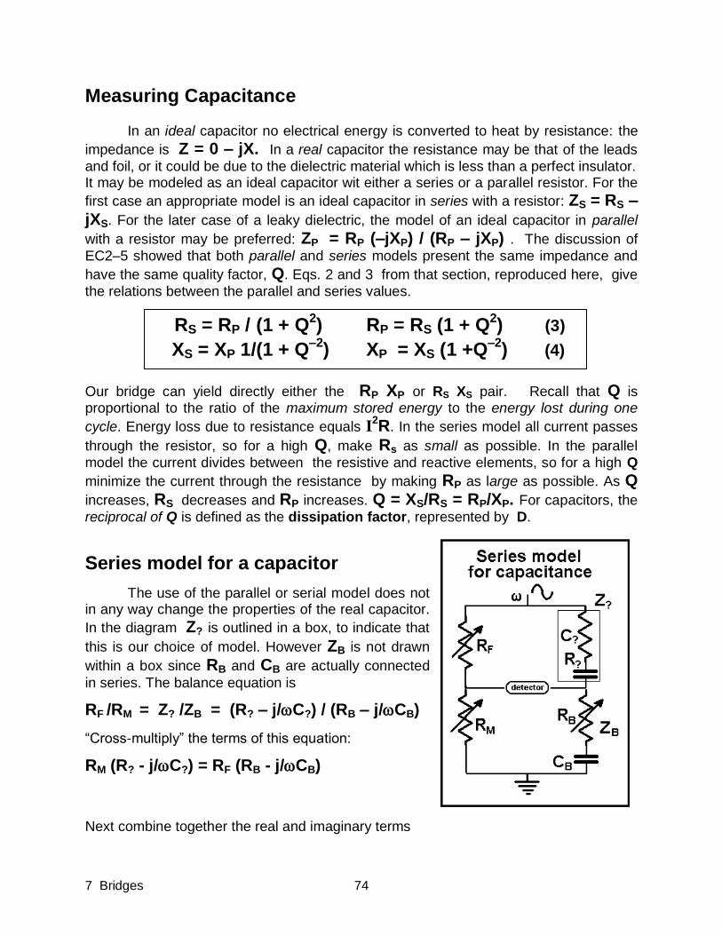
7 Bridges 74
Measuring Capacitance
In an ideal capacitor no electrical energy is converted to heat by resistance: the
impedance is Z = 0 – jX. In a real capacitor the resistance may be that of the leads
and foil, or it could be due to the dielectric material which is less than a perfect insulator. It may be modeled as an ideal capacitor wit either a series or a parallel resistor. For the
first case an appropriate model is an ideal capacitor in series with a resistor: ZS = RS – jXS. For the later case of a leaky dielectric, the model of an ideal capacitor in parallel
with a resistor may be preferred: ZP = RP (–jXP) / (RP – jXP) . The discussion of
EC2–5 showed that both parallel and series models present the same impedance and
have the same quality factor, Q. Eqs. 2 and 3 from that section, reproduced here, give
the relations between the parallel and series values.
Our bridge can yield directly either the RP XP or RS XS pair. Recall that Q is proportional to the ratio of the maximum stored energy to the energy lost during one
cycle. Energy loss due to resistance equals I2R. In the series model all current passes
through the resistor, so for a high Q, make Rs as small as possible. In the parallel
model the current divides between the resistive and reactive elements, so for a high Q
minimize the current through the resistance by making RP as large as possible. As Q
increases, RS decreases and RP increases. Q = XS/RS = RP/XP. For capacitors, the
reciprocal of Q is defined as the dissipation factor, represented by D.
Series model for a capacitor
The use of the parallel or serial model does not in any way change the properties of the real capacitor.
In the diagram Z? is outlined in a box, to indicate that
this is our choice of model. However ZB is not drawn
within a box since RB and CB are actually connected
in series. The balance equation is
RF /RM = Z? /ZB = (R? – j/C?) / (RB – j/CB)
“Cross-multiply” the terms of this equation:
RM (R? - j/C?) = RF (RB - j/CB)
Next combine together the real and imaginary terms
RS = RP / (1 + Q2) RP = RS (1 + Q
2) (3)
XS = XP 1/(1 + Q–2
) XP = XS (1 +Q–2
) (4)
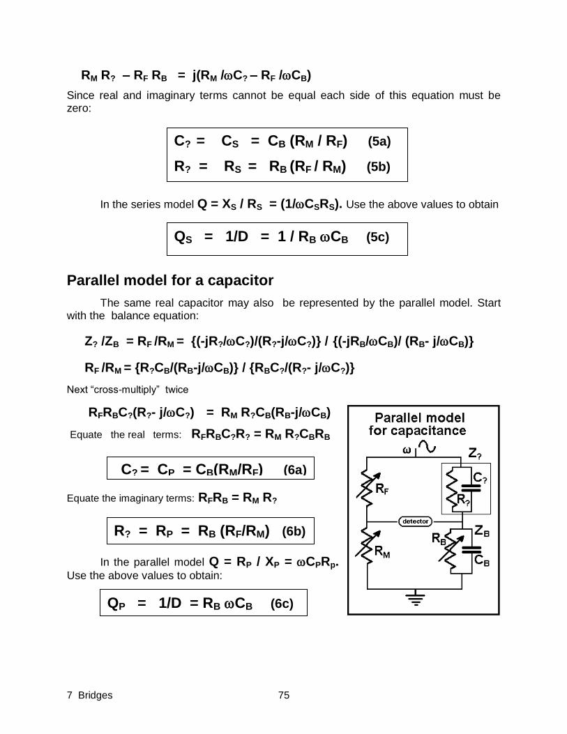
7 Bridges 75
RM R? – RF RB = j(RM /C? – RF /CB)
Since real and imaginary terms cannot be equal each side of this equation must be zero:
In the series model Q = XS / RS = (1/CSRS). Use the above values to obtain
Parallel model for a capacitor
The same real capacitor may also be represented by the parallel model. Start with the balance equation:
Z? /ZB = RF /RM = {(-jR?/C?)/(R?-j/C?)} / {(-jRB/CB)/ (RB- j/CB)}
RF /RM = {R?CB/(RB-j/CB)} / {RBC?/(R?- j/C?)}
Next “cross-multiply” twice
RFRBC?(R?- j/C?) = RM R?CB(RB-j/CB)
Equate the real terms: RFRBC?R? = RM R?CBRB
Equate the imaginary terms: RFRB = RM R?
In the parallel model Q = RP / XP = CPRp. Use the above values to obtain:
C? = CS = CB (RM / RF) (5a)
R? = RS = RB (RF / RM) (5b)
C? = CP = CB(RM/RF) (6a)
R? = RP = RB (RF/RM) (6b)
QS = 1/D = 1 / RB CB (5c)
QP = 1/D = RB CB (6c)

7 Bridges 76
Practical considerations
For a real capacitor a Q value of 100 or more is typical (corresponding to a
dissipation factor, D, of 0.01 or less). For such a case Eq. (4) indicates that XP and XS differ by only 0.01% . Therefore the capacitance may be measured, using either the
parallel or series bridge configuration. However Eq, (3) shows RP to be 10,000 times
RS. This is of some concern.
Notice that the unknown R? and C? results are independent of the angular
frequency However the required value of the balance resistor, RB, does depend on
and also Q. Suppose we are to measure a 0.47 microfarad capacitor with a Q of
200 at 2.00 kHz. Take CB = 100.0 nf . From either Eq. (5a) or (6a) we find that
(RM/RF) = 4.70. With the serial configuration, RB ≈ 4and with the parallel
configuration RB ≈ 159kThis is a problem since the adjustable resistance on the
module, RB, has a maximum of 25kand it is quite difficult to adjust it accurately to
just 4 ohms.
There is a way to work around this limitation. For any capacitor, Q = 1(RC).
Consider a 0.47f capacitor with 4series resistance at 2.00 kHz. Its Q is
approximately 200. Add in series a 25 resistor (adjust Radd) and Q drops from 200
to approximately 27 (XS and XP remain practically unchanged). However the series and
parallel mode RB values required for balance now become 29 and 22k which can be
provided by the bridge components. So if a parallel balance cannot be attained even
with the maximum RB setting, add sufficient Radd in series with C?? to attain balance
Near balance the detector voltage can be quite small, a small fraction of a
millivolt. When a sinusoidal voltage is used, the 60 hertz line voltage could cause appreciable interference at these low levels, and also high frequency oscillations tend to appear. To eliminate these problems a parallel L-C circuit, tuned to 2.0 kHz is inserted across the Detector when the AC / DC switch is set in the AC position
For inductors and capacitors, both RM and RB must be continuously adjusted to
obtain balance. It is a convenient procedure to set to zero the x1, x10 and x100 ranges
of the decade resistor, RM, and adjust only the x1000 range. If a minimum detector
level is not found somewhere in this range for any value of RB,, select a different RF
resistor. Once a minimum level is found on the x1000 range move to the next lower
range and find there the next minimum by further adjustment of RM and RB .

7 Bridges 77
Parallel model for an Inductor
As with capacitors, any real inductor may be modeled by an ideal inductor in series or parallel with a resistor. With our bridge circuits to use the serial model
for a capacitors, Z?, we also set ZB in the serial
configuration. Likewise for the parallel model of Z? we set
ZB in parallel mode. But this is not so for inductors. There is simply no solution for the inductor balance equation if
Z? and ZB are both expressed as serial or both expressed as parallel. This is because we are balancing a
real inductor with a capacitor. The ZB of our bridge cannot
be made inductive.
Activity 7-2 Measuring Capacitance
1: To the AC / DC input connect a function generator set to 2,000 hz, sine wave, maximum amplitude.. To the Detector terminals connect an oscilloscope, set for AC input. Vertical gain may be increased as the exact balance condition is approached. Set AC / DC switch to AC
To the RM terminals connect a 0-9,999 decade resistor. Connect an ohmmeter to the RB terminals to measure its variable setting To the terminal marked A connect the free end of the RF resistor, as selected.
2: Set the Measure RB -Operate switch to Operate Set the Parallel - Series switch to Parallel. Set the capacitor selection switch to 100 nf Attach to the C?? input capacitor C-1 in series with Radd . Use the minimum setting of Radd (full counter clockwise) and balance the bridge by adjusting both RM and RB and possibly Radd to obtain a minimum Detector output
Record RM, RF and measure RB and Radd
Calculate RP , CP and QP using Eq.(6).
3: Radd Set the Parallel - Series switch to Series Do not change the Radd Balance the bridge. Record RM, RF and measure RB Calculate RS , CS and QS using Eq.(5).
4: Assign Q as ½(QS + QP) Using this Q calculate CS/CP and Rp/RS and compare these values with the theoretical values given by Eqs. (3, 4).
5: Repeat steps 2,3,4. but use C-2 in place of C-1 and select CB to give the best value.

7 Bridges 78
L? = LP = [RMRF] CB (7a)
L? = LS = [RM RF] CB (8a)
R? = RS = [RM RF] / RB (8b)
Start with the inductor balance equation:
Z? / RM = RF / ZB
{jR? L? /(R? + jL?)} / RM = RF/(RB – j/CB)
Multiply each side by RM and then “cross-multiply”
jR? L? (RB – j/CB) = RM RF(R? + jL?)
jR? RBL? + R? L? /CB = RMRFR? + jRMRFL?
Equate the real terms:
R? L? /CB = RMRFR?
Equate the imaginary terms to obtain:
jR? RBL? = jRMRFL?
For the parallel model Q = RP / XP so
Q = {[RMRF] / RB} / [RMRF] CB
Serial model for an Inductor Since the serial model is to be used for Z? then
the parallel setting is to be used for ZB .Otherwise no
solution for the balance equation can be found. Start
with the balance equation: Z? / RM = RF / ZB
(R? + jL?) / RM = RF/{(-jRB/CB) / (RB - j/CB)}
(R? + jL?) / RM = RF (RB - j/CB) / (- jRB/CB)
“Cross-multiply”, to obtain:
(R? + jL?) (- jRB/CB) = RM RF (RB - j/CB)
Equate the real terms to obtain
L? RB/CB = RM RF RB or Equate the imaginary terms to obtain
R? RB/CB = RM RF /CB or
R? = RP = [RMRF] / RB (7b)
QP = 1/(CB RB) (7C)
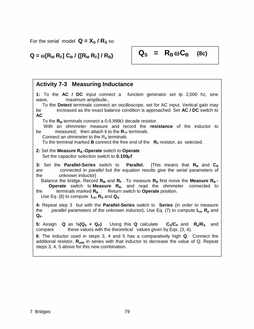
7 Bridges 79
QS = RB CB (8c)
For the serial model Q = XS / RS so
Q = [RM RF] CB / {[RM RF] / RB}
Activity 7-3 Measuring Inductance
1: To the AC / DC input connect a function generator set tp 2,000 hz, sine wave, maximum amplitude.. To the Detect terminals connect an oscilloscope, set for AC input. Vertical gain may be increased as the exact balance condition is approached. Set AC / DC switch to AC
To the RM terminals connect a 0-9,999 decade resistor. With an ohmmeter measure and record the resistance of the inductor to be measured; then attach it to the R?? terminals. Connect an ohmmeter to the RB terminals To the terminal marked B connect the free end of the RF resistor, as selected.
2: Set the Measure RB -Operate switch to Operate
Set the capacitor selection switch to 0.100f
3: Set the Parallel-Series switch to Parallel. [This means that RB and CB are connected in parallel but the equation results give the serial parameters of the unknown inductor] Balance the bridge. Record RM and RF . To measure RB first move the Measure RB - Operate switch to Measure RB, and read the ohmmeter connected to the terminals marked RB . Return switch to Operate position. Use Eq. (8) to compute LS, RS and QS.
4: Repeat step 3 but with the Parallel-Series switch to Series (in order to measure the parallel parameters of the unknown inductor). Use Eq. (7) to compute Lp, Rp and QP.
5: Assign Q as ½(QS + QP) Using this Q calculate CS/CP and Rp/RS and compare these values with the theoretical values given by Eqs. (3, 4).
6: The inductor used in steps 3, 4 and 5 has a comparatively high Q. Connect the additional resistor, Radd in series with that inductor to decrease the value of Q. Repeat steps 3, 4, 5 above for this new combination.

7 Bridges 80
Data Sheet Experiment # EC2-7
Bridges
Name ______________________________ Date__________
Activity 7-1: Measuring Resistance
With R-1
RB 10 10 10 100 100 100 1k 1k 1k
RF 100 1k 10k 100 1k 10k 100 1k 10k
RM
R?
R-1 ________ R-2 ________ R-3 ________ Rseries ____________ (R-2 + R-3) ______________ Rparallel __________ (R-2 x R-3)/ (R-2 + R-3) ____________
Activity 7-2: Measuring Capacitance
For C-1 CB = 100.0 nf f ________
Parallel: RM ________ RF_________ RB_________ Radd __________
CP __________ RP___________ Q P _____________
Series: RM ____________ RF____________ RB___________
CS ______________ RS___________ Q S ____________
Q = ½ (QS + Qp) ________
CS/ CP ___________ (1 + Q–2
) _____________
RP / RS ___________ (1 + Q2) _____________
For C-2 CB __________ f ________
Parallel: RM ________ RF_________ RB_________ Radd __________
CP __________ RP___________ Q P _____________
Series: RM ____________ RF____________ RB___________
CS ______________ RS___________ Q S ____________
Q = ½ (QS + Qp) ________
CS/ CP ___________ (1 + Q–2
) _____________
RP / RS ___________ (1 + Q2) _____________
7 Bridges 81
Data Sheet Experiment # EC2-7, continued Activity 7-3: Measuring Inductance DC inductor resistance __________ Without Radd
Series: RM __________ RF__________ RB_________ CB ____________
LS ____________ RS___________ Q S ____________
Parallel: RM __________ RF__________ RB_________ CB ____________
LP ____________ RP___________ Q P _____________
Q = ½ (QS + Qp) ________
LP/LS ___________ (1 + Q–2
) _____________
RP / RS ___________ (1 + Q2) _____________
With Radd included
Series: RM __________ RF__________ RB_________ CB ____________
LS ____________ RS___________ Q S ____________
Parallel: RM __________ RF__________ RB_________ CB ____________
LP ____________ RP___________ Q P _____________
Q = ½ (QS + Qp) ________
LP/LS ___________ (1 + Q–2
) _____________
RP / RS ___________ (1 + Q2) _____________

7 Bridges 82
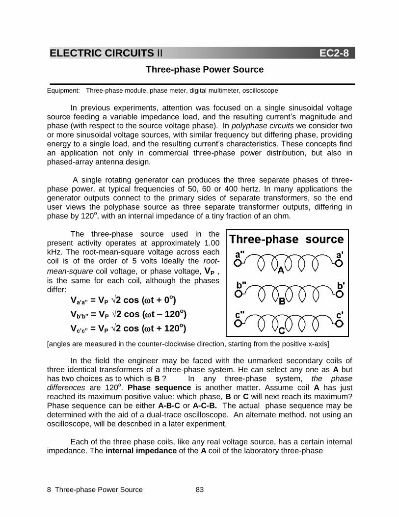
8 Three-phase Power Source 83
Three-phase Power Source
Equipment: Three-phase module, phase meter, digital multimeter, oscilloscope
In previous experiments, attention was focused on a single sinusoidal voltage source feeding a variable impedance load, and the resulting current’s magnitude and phase (with respect to the source voltage phase). In polyphase circuits we consider two or more sinusoidal voltage sources, with similar frequency but differing phase, providing energy to a single load, and the resulting current’s characteristics. These concepts find an application not only in commercial three-phase power distribution, but also in phased-array antenna design. A single rotating generator can produces the three separate phases of three-phase power, at typical frequencies of 50, 60 or 400 hertz. In many applications the generator outputs connect to the primary sides of separate transformers, so the end user views the polyphase source as three separate transformer outputs, differing in phase by 120o, with an internal impedance of a tiny fraction of an ohm. The three-phase source used in the present activity operates at approximately 1.00 kHz. The root-mean-square voltage across each coil is of the order of 5 volts Ideally the root-
mean-square coil voltage, or phase voltage, VP , is the same for each coil, although the phases differ:
Va’a” = VP √2 cos (t + 0o)
Vb’b” = VP √2 cos (t – 120o)
Vc’c” = VP √2 cos (t + 120o)
[angles are measured in the counter-clockwise direction, starting from the positive x-axis]
In the field the engineer may be faced with the unmarked secondary coils of three identical transformers of a three-phase system. He can select any one as A but has two choices as to which is B ? In any three-phase system, the phase differences are 120o. Phase sequence is another matter. Assume coil A has just reached its maximum positive value: which phase, B or C will next reach its maximum? Phase sequence can be either A-B-C or A-C-B. The actual phase sequence may be determined with the aid of a dual-trace oscilloscope. An alternate method. not using an oscilloscope, will be described in a later experiment. Each of the three phase coils, like any real voltage source, has a certain internal impedance. The internal impedance of the A coil of the laboratory three-phase
ELECTRIC CIRCUITS II EC2-8
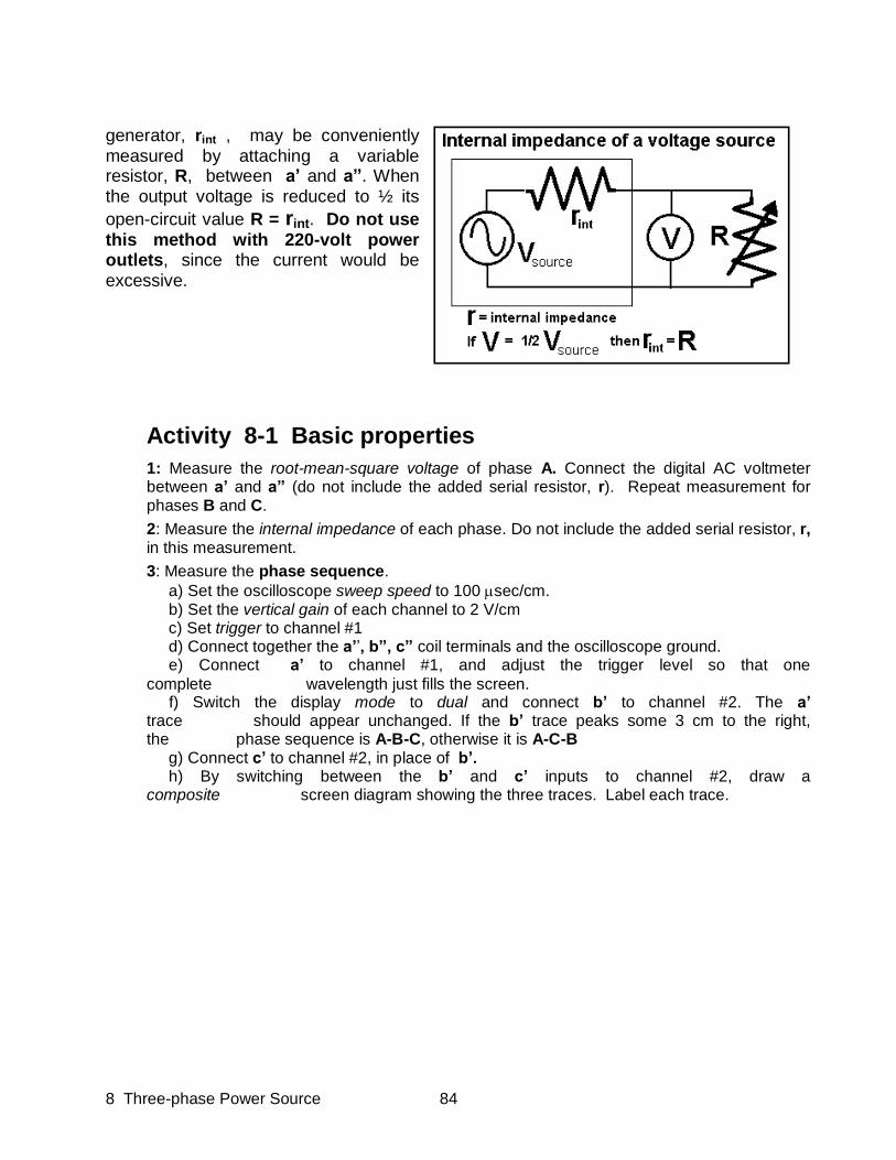
8 Three-phase Power Source 84
generator, rint , may be conveniently measured by attaching a variable resistor, R, between a’ and a”. When the output voltage is reduced to ½ its
open-circuit value R = rint. Do not use this method with 220-volt power outlets, since the current would be excessive.
Activity 8-1 Basic properties
1: Measure the root-mean-square voltage of phase A. Connect the digital AC voltmeter between a’ and a” (do not include the added serial resistor, r). Repeat measurement for phases B and C.
2: Measure the internal impedance of each phase. Do not include the added serial resistor, r, in this measurement.
3: Measure the phase sequence.
a) Set the oscilloscope sweep speed to 100 sec/cm. b) Set the vertical gain of each channel to 2 V/cm c) Set trigger to channel #1 d) Connect together the a’’, b”, c” coil terminals and the oscilloscope ground. e) Connect a’ to channel #1, and adjust the trigger level so that one
complete wavelength just fills the screen. f) Switch the display mode to dual and connect b’ to channel #2. The a’ trace should appear unchanged. If the b’ trace peaks some 3 cm to the right, the phase sequence is A-B-C, otherwise it is A-C-B g) Connect c’ to channel #2, in place of b’. h) By switching between the b’ and c’ inputs to channel #2, draw a composite screen diagram showing the three traces. Label each trace.

8 Three-phase Power Source 85
Connecting just two phases Two identical dry cells may be connected in series in two ways, aiding or opposing. With sinusoidal sources, even if
the amplitude, VP , and angular frequency, are the same, yet the sum depends on their
phase difference, . For = 0, the amplitude
of their sum is 2 while for = 180o it is zero. [See Notes on Trigonometry, Eq .(14)]
As a first step, connect together only two phases, A and B. Although their amplitude and frequency are identical and the differ in phase by 120o , yet there are two wats to connect them in series. One way is to connect together a” and b” terminals, as shown.
We expect the measured rms voltage across each coil to be equal; |VA| = |VB| =
VP, the common coil or phase voltage. Phasors for the A and B coils, connected as
shown, Va’a” and Vb’b” , are drawn with a
common origin, of equal length, and differ in direction by 1200 . Assume the phase sequence to be A-B-C. The voltmeter
reading, |VA–VB| is Va’b’. It is convenient to
select Va’a” as the reference direction. Then
we find:
Va’a” = VP 0o = VP [ cos 0o + j sin 0o ]
= VP [ 1 + j 0]
Vb’b” = VP –120o
= VP [ cos –120o + j sin –120o ] = VP [ –0.500 – j 0.866]
Va’b’ = VP [ 1.500 + j 0.866]
= 31/2 VP 30o
The magnitude of these three phasors may be verified with an AC digital voltmeter, but an oscilloscope or phase meter is needed to verify the angles. With the
oscilloscope connect the common ground to a’ , connect channel #1 to a” and
channel #2 to b’ and change rthe for channel #2.
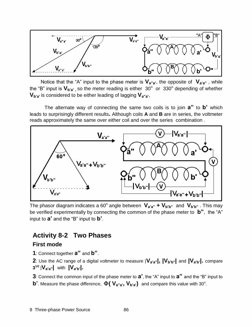
8 Three-phase Power Source 86
Notice that the “A” input to the phase meter is Va”a’, the opposite of Va’a” , while
the “B” input is Vb’a’ , so the meter reading is either 30o or 330o depending of whether
Vb’a’ is considered to be either leading of lagging Va”a’,
The alternate way of connecting the same two coils is to join a” to b’ which
leads to surprisingly different results. Although coils A and B are in series, the voltmeter
reads approximately the same over either coil and over the series combination .
The phasor diagram indicates a 60o angle between Va’a” + Vb’b” and Vb’b” . This may
be verified experimentally by connecting the common of the phase meter to b”, the “A”
input to a’ and the “B” input to b’.
Activity 8-2 Two Phases
First mode
1: Connect together a” and b”.
2: Use the AC range of a digital voltmeter to measure |Va’a”|, |Vb’b”| and |Va’b’|. compare
31/2 |Va’a”| with |Va’b’|.
3: Connect the common input of the phase meter to a’, the “A” input to a” and the “B” input to
b’. Measure the phase difference, ( Va”a’, Vb’a’) and compare this value with 30o.
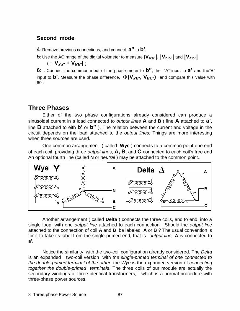
8 Three-phase Power Source 87
Three Phases
Either of the two phase configurations already considered can produce a
sinusoidal current in a load connected to output lines A and B ( line A attached to a’, line B attached to eith b’ or b” ). The relation between the current and voltage in the circuit depends on the load attached to the output lines. Things are more interesting when three sources are used.
One common arrangement ( called Wye ) connects to a common point one end
of each coil providing three output lines, A, B, and C connected to each coil’s free end
An optional fourth line (called N or neutral ) may be attached to the common point..
Another arrangement ( called Delta ) connects the three coils, end to end, into a
single loop, with one output line attached to each connection. Should the output line attached to the connection of coil A and B be labeled A or B ? The usual convention is for it to take its label from the single primed end, that is output line A is connected to a’.
Notice the similarity with the two-coil configuration already considered. The Delta is an expanded two-coil version with the single-primed terminal of one connected to the double-primed terminal of the other; the Wye is the expanded version of connecting together the double-primed terminals. The three coils of our module are actually the secondary windings of three identical transformers, which is a normal procedure with three-phase power sources.
Second mode
4: Remove previous connections, and connect a” to b’.
5: Use the AC range of the digital voltmeter to measure |Va’a”|, |Vb’b”| and |Va’b”| ( = |Va’a” + Vb’b”| ).
6: : Connect the common input of the phase meter to b”, the “A” input to a’ and the”B”
input to b’. Measure the phase difference, (Va’b”, Vb’b”) and compare this value with
60o.

8 Three-phase Power Source 88
When we examine the source side, each coil or transformer secondary winding has a definite voltage across it, and may have its own current, dependent on external connections: these are called phase voltages and currents. Looking at the line side,
definite voltages exist between the lines , as VAB, VCN, etc., and are called line voltages. Depending on any external load there may be currents in individual lines, called line currents. For line voltages the order of subscripts is significant. For
example, VAB = –VBA and, as phasors, they have the same magnitude but point in
opposire directions. In many applications, where the load is reasonably balanced and the source impedance is quite low, the phase voltages have the same magnitude
independent of current: |Va’a”| = |Vb’b”| = |Vc’c”| = |Vp| .
If there is no load (line currents are zero) clearly in the Wye configuration there will be no phase currents But what about the Delta configuration where the three coils form a continuous loop?
A phase diagram of the voltages in the Delta configuration shows that the sum of any two phase voltages just balances out the third phase so the sum of the voltages around the Delta loop just equals zero. Actually, if the loop is opened at any node and an AC voltmeter inserted, the voltage is almost, but not quite, zero. If an oscilloscope is used in place of the voltmeter, the small voltage is seen to have a frequency of about 3,000 hz, a third-harmonic produced by a slight non-linearity in the transformer cores. While the fundamentals of the three phase voltages are 120o apart, the phase differences of the third harmonics are 3 x 120o or 360o apart. Therefore they do not cancel but rather add. However with well designed transformers this third harmonic component is quite small
With algebra we can show that the phasor sum of the three coil voltages is zero:
Va’a” = Vphase 0o = Vphase [1.00 + j 0.000 ]
Vb’b” = Vphase –120o = Vphase [–0.500 – j 0.866 ]
Vc’c” = Vphase +120o = Vphase [–0.500 + j 0.866 ]
Sum = Vphase [0.000 + j 0.000 ]

8 Three-phase Power Source 89
Line voltages with a Wye source
In the Wye configuration with any load attached each of the three line currents must always equal the corresponding phase currents since the line and phase are directly connected. In the four-wire Wye connection we may consider the voltage
between A, B or C lines and the N ( for neutral) line, VAN, VBN, VCN . It is clear from
the Wye diagram that each of these equals the corresponding phase voltage:
VAN = Va’n VBN = Vb’n VCN = Vc’n
We may also consider the voltages between the lines, or line voltages, VAB , VBC or
VCA. Each of these have contributions from two phase voltages differing by 120o. The
line voltage, VAB, is the series combination of Va’n and Vnb’. The phasor diagram
above shows this relation, which is confirmed by algebra:
Va’n = Vphase 0o = Vphase [1 + j 0]
Vb’n = Vphase –120o = Vphase [–0.500 – j 0.866 ]
VAB = Va’n – Vb’n = Vphase [1.500 + j 0.866 ] = 31/2
Vphase 30o
Similar results hold for VBC and VCA. In the Wye configuration line voltages are larger
than the phase voltages by a factor of the square root of three. The AB line voltage lags
Va’n by 30o and leads Vc’n by 90o
Line currents with a Delta source
With a Delta source, the line voltages equal the corresponding phase voltages. To have line currents, there must a load. If the load is balanced, ( the same impedance between each pair of lines ) the line currents must be symetric, that is, each have the same magnitude and differ in phase by 120o. Of course both line and phase currents depend on the characteristics of the load. But for any symetrical load we ask about the relation between line and phase currents in a Delta configuration.
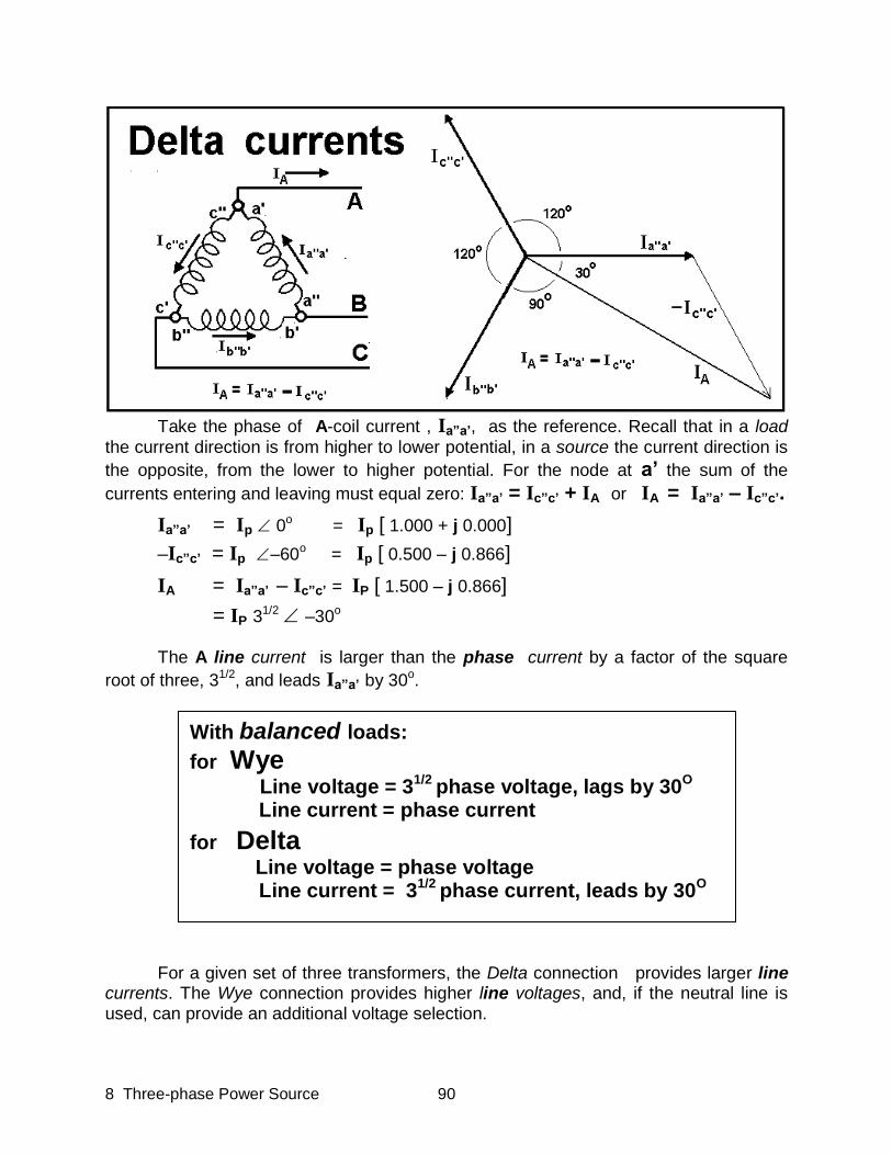
8 Three-phase Power Source 90
Take the phase of A-coil current , Ia”a’, as the reference. Recall that in a load
the current direction is from higher to lower potential, in a source the current direction is
the opposite, from the lower to higher potential. For the node at a’ the sum of the
currents entering and leaving must equal zero: Ia”a’ = Ic”c’ + IA or IA = Ia”a’ – Ic”c’.
Ia”a’ = Ip 0o = Ip [ 1.000 + j 0.000]
–Ic”c’ = Ip –60o = Ip [ 0.500 – j 0.866]
IA = Ia”a’ – Ic”c’ = IP [ 1.500 – j 0.866]
= IP 31/2 –30o
The A line current is larger than the phase current by a factor of the square
root of three, 31/2, and leads Ia”a’ by 30o.
For a given set of three transformers, the Delta connection provides larger line currents. The Wye connection provides higher line voltages, and, if the neutral line is used, can provide an additional voltage selection.
With balanced loads:
for Wye
Line voltage = 31/2
phase voltage, lags by 30O
Line current = phase current
for Delta
Line voltage = phase voltage Line current = 3
1/2 phase current, leads by 30
O
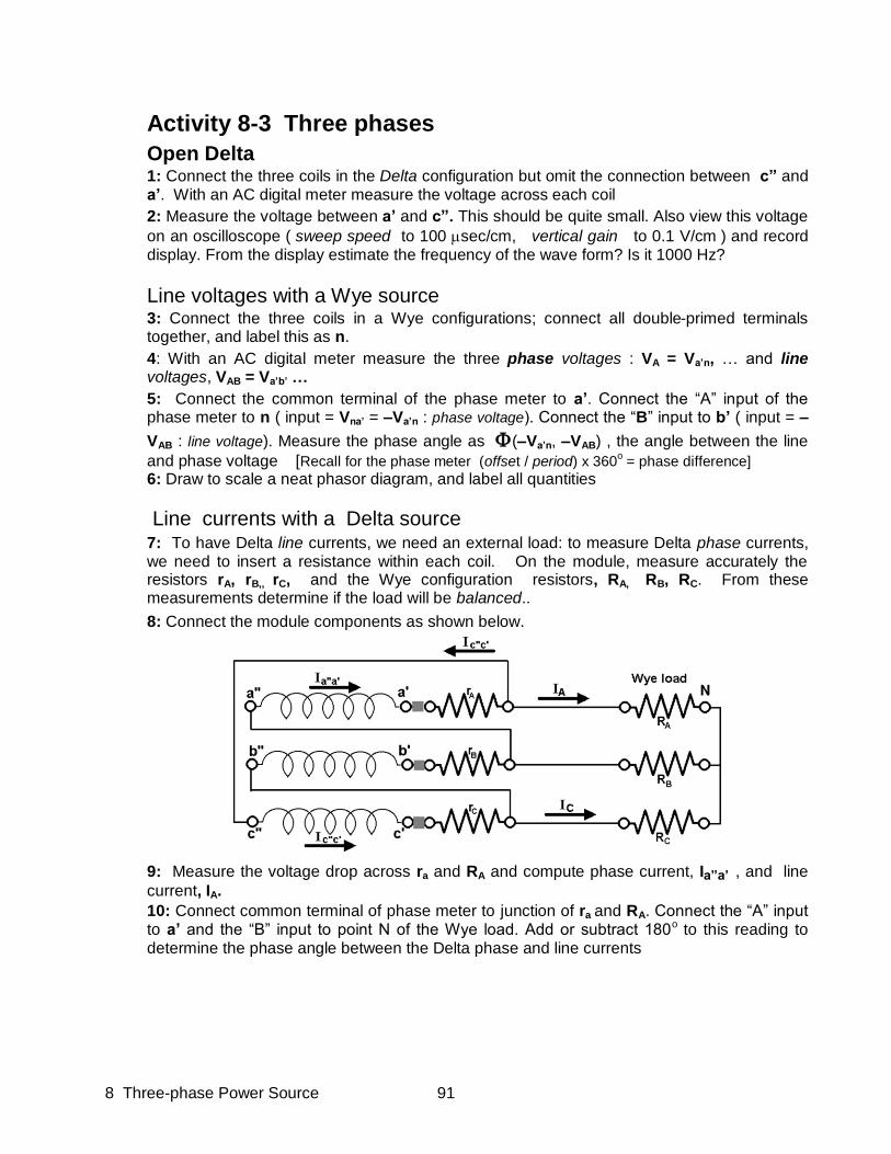
8 Three-phase Power Source 91
Activity 8-3 Three phases
Open Delta
1: Connect the three coils in the Delta configuration but omit the connection between c” and a’. With an AC digital meter measure the voltage across each coil
2: Measure the voltage between a’ and c”. This should be quite small. Also view this voltage
on an oscilloscope ( sweep speed to 100 sec/cm, vertical gain to 0.1 V/cm ) and record display. From the display estimate the frequency of the wave form? Is it 1000 Hz?
Line voltages with a Wye source
3: Connect the three coils in a Wye configurations; connect all double-primed terminals together, and label this as n.
4: With an AC digital meter measure the three phase voltages : VA = Va’n, … and line voltages, VAB = Va’b’ …
5: Connect the common terminal of the phase meter to a’. Connect the “A” input of the phase meter to n ( input = Vna’ = –Va’n : phase voltage). Connect the “B” input to b’ ( input = –
VAB : line voltage). Measure the phase angle as (–Va’n, –VAB) , the angle between the line
and phase voltage [Recall for the phase meter (offset / period) x 360o = phase difference]
6: Draw to scale a neat phasor diagram, and label all quantities
Line currents with a Delta source
7: To have Delta line currents, we need an external load: to measure Delta phase currents, we need to insert a resistance within each coil. On the module, measure accurately the resistors rA, rB,, rC, and the Wye configuration resistors, RA, RB, RC. From these measurements determine if the load will be balanced..
8: Connect the module components as shown below.
9: Measure the voltage drop across ra and RA and compute phase current, Ia”a’ , and line
current, IA.
10: Connect common terminal of phase meter to junction of ra and RA. Connect the “A” input to a’ and the “B” input to point N of the Wye load. Add or subtract 180o to this reading to determine the phase angle between the Delta phase and line currents
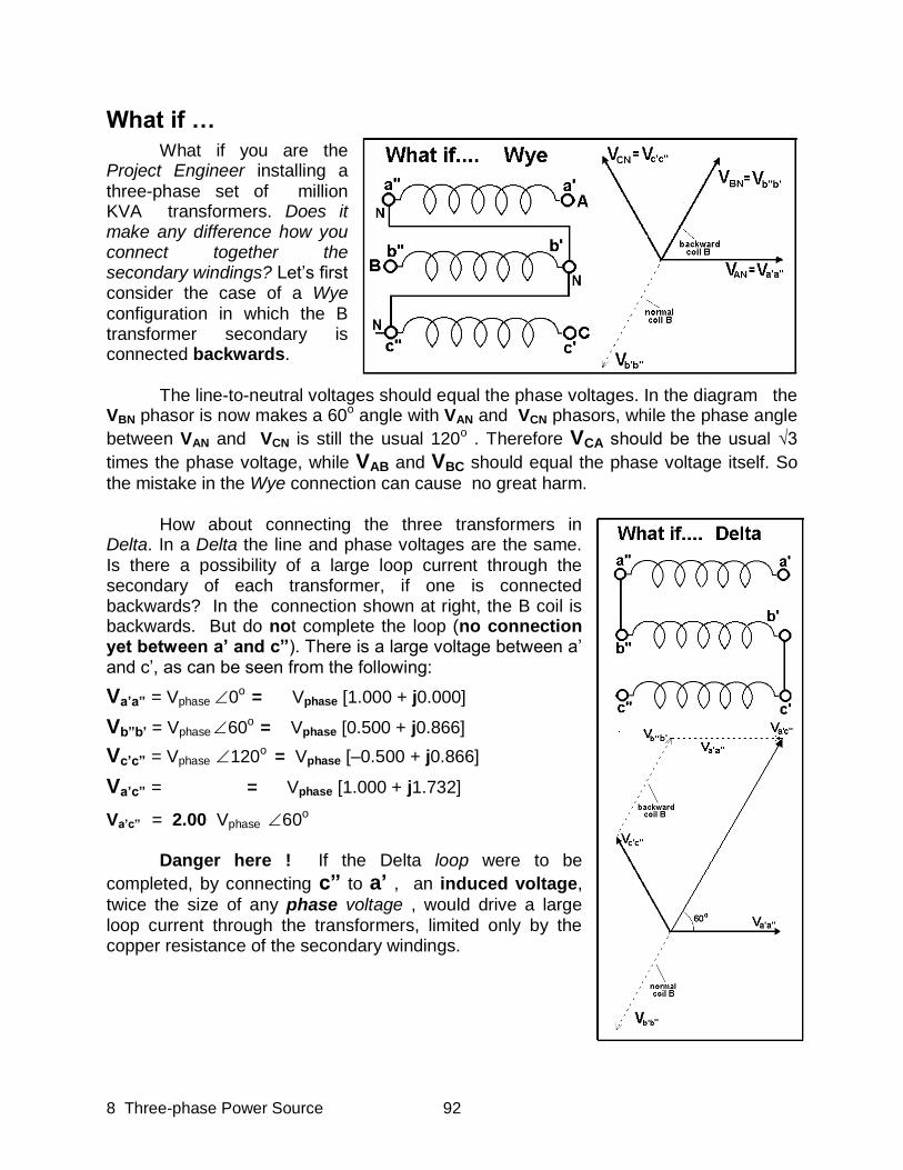
8 Three-phase Power Source 92
What if …
What if you are the Project Engineer installing a three-phase set of million KVA transformers. Does it make any difference how you connect together the secondary windings? Let’s first consider the case of a Wye configuration in which the B transformer secondary is connected backwards. The line-to-neutral voltages should equal the phase voltages. In the diagram the VBN phasor is now makes a 60o angle with VAN and VCN phasors, while the phase angle
between VAN and VCN is still the usual 120o . Therefore VCA should be the usual √3
times the phase voltage, while VAB and VBC should equal the phase voltage itself. So
the mistake in the Wye connection can cause no great harm. How about connecting the three transformers in Delta. In a Delta the line and phase voltages are the same. Is there a possibility of a large loop current through the secondary of each transformer, if one is connected backwards? In the connection shown at right, the B coil is backwards. But do not complete the loop (no connection yet between a’ and c”). There is a large voltage between a’ and c’, as can be seen from the following:
Va’a” = Vphase 0o = Vphase [1.000 + j0.000]
Vb”b’ = Vphase 60o = Vphase [0.500 + j0.866]
Vc’c” = Vphase 120o = Vphase [–0.500 + j0.866]
Va’c” = = Vphase [1.000 + j1.732]
Va’c” = 2.00 Vphase 60o
Danger here ! If the Delta loop were to be
completed, by connecting c” to a’ , an induced voltage,
twice the size of any phase voltage , would drive a large loop current through the transformers, limited only by the copper resistance of the secondary windings.

8 Three-phase Power Source 93
Activity 8-4 What if…
Wye:
1: Measure the phase voltages |Va’a”|, |Vb’b”|, |Vc’c”| and line voltages |VAB|, |VBC|, |VCA| . Compare VCA with √3 phase voltage. CA
2: Connect the phase meter common terminal to N, the “A” input to a’, the “B” input to b” and
measure (Va’N, Vb’N) and compare with 60o.
3: Connect the phase meter common terminal to N, the “A” input to c’, the “B” input to a’ and
measure ( Vc’N, Va’N) and compare with 120o.
Delta:
4: Measure the three phase voltages |Va’a” |, |Vb’b”|, |Vc’c”|. Also measure |Va’c”| , the
voltage between the open terminals a’ and c”
5: Connect the phase meter common terminal to a’, the ”A” input to a”, the “B” input to c”
and measure (–Va’a”,–Vc”a’) and compare with 60o.

8 Three-phase Power Source 94
Data Sheet Experiment # EC2-8 Three-phase Power Source
Name ______________________________ Date__________
Activity 8-1: Basic properties
Vrms: A _________ B _________ C ________
Internal Impedance: A ________ B ________ C ________ Phase sequence: [ ] A-B-C , [ ] A-C-B
sweep speed: 100 sec/cm vertical gain : 2 V/cm
Activity 8-2 Two Phases
a” connected to b”
|Va’a”| _______ |Vb’b”| ______ |Va’b’| _______ 31/2
|Va’a”| _________
( Va”a’, Vb’a’) ___________
a” connected to b’
|Va’a”| __________ |Vb’b”| ___________ |Va’b”| ___________
(Va’b”, Vb’b”) ___________
Data Sheet Experiment # EC2-8 (continued)

8 Three-phase Power Source 95
Activity 8-3 Three phases
Open Delta: |Va’a”| __________
|Vb’b”| __________
|Vc’c”| __________
|Va’c” | __________
sweep speed : 100 sec/cm vertical gain: 0.1 V/cm
estimated frequency _________
Line voltages with a Wye source
|Va’n| _____ |Vb’n| _____ |Vc’n| _____
|Va’b’| _____ |Vb’c’| _____ |Vc’a| _____
(–Va’n, –VAB) _________
Line currents with a Delta source
rA _____ rB _______, rC _______
RA _____ RB ______ RC ________
Is the load balanced? ______
|VRa| _____ |IA| ______
|Vra| _____ |Ia”a’| ______
angle between phase and line current :
( Ia”a’, –IA) ________

8 Three-phase Power Source 96
Data Sheet Experiment # EC2-8 (continued)
Activity 8-4 What if…
Wye
|Va’a” | _______ |Vb’b”| _______ |Vc’c”| _________
|VAB | _______ |VBC| _______ |VCA| _________
(Va’N, Vb’N) _______ ( Vc’N, Va’N) _______
Delta
|Va’a” | _______ |Vb’b”| ______ |Vc’c”| _______ |Va’c”| ___________
(–Va’a”, –Vc”a’) ________
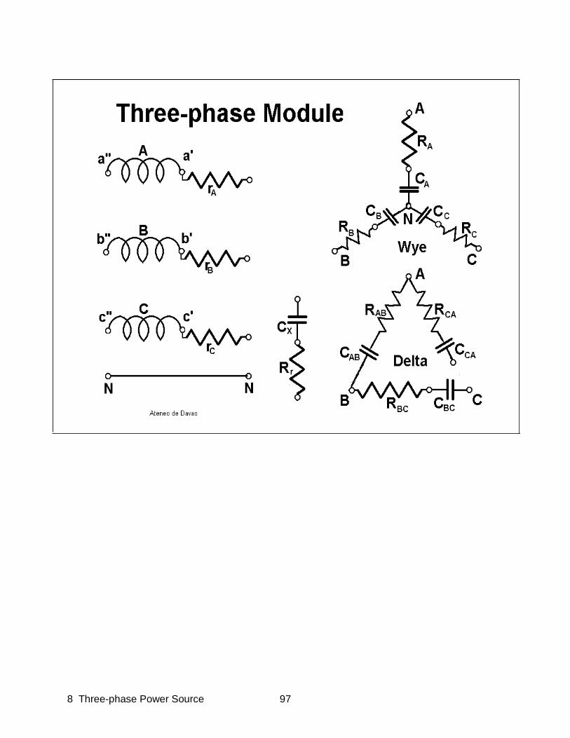
8 Three-phase Power Source 97
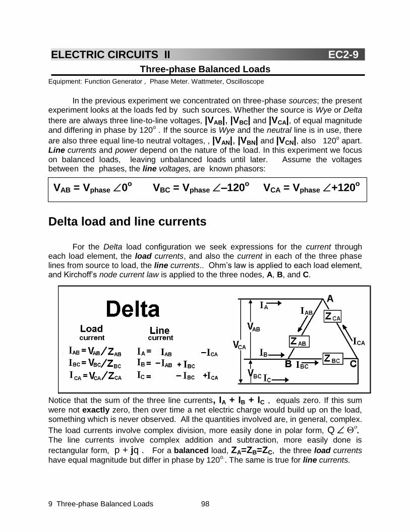
9 Three-phase Balanced Loads 98
Three-phase Balanced Loads
Equipment: Function Generator , Phase Meter. Wattmeter, Oscilloscope
In the previous experiment we concentrated on three-phase sources; the present experiment looks at the loads fed by such sources. Whether the source is Wye or Delta
there are always three line-to-line voltages, |VAB|, |VBC| and |VCA|, of equal magnitude
and differing in phase by 120o . If the source is Wye and the neutral line is in use, there
are also three equal line-to neutral voltages, , |VAN|, |VBN| and |VCN|, also 120o apart. Line currents and power depend on the nature of the load. In this experiment we focus on balanced loads, leaving unbalanced loads until later. Assume the voltages between the phases, the line voltages, are known phasors:
Delta load and line currents
For the Delta load configuration we seek expressions for the current through each load element, the load currents, and also the current in each of the three phase lines from source to load, the line currents.. Ohm’s law is applied to each load element, and Kirchoff’s node current law is applied to the three nodes, A, B, and C.
Notice that the sum of the three line currents, IA + IB + IC , equals zero. If this sum
were not exactly zero, then over time a net electric charge would build up on the load, something which is never observed. All the quantities involved are, in general, complex.
The load currents involve complex division, more easily done in polar form, Q
The line currents involve complex addition and subtraction, more easily done is
rectangular form, p + jq . For a balanced load, ZA=ZB=ZC, the three load currents
have equal magnitude but differ in phase by 120o.. The same is true for line currents.
ELECTRIC CIRCUITS II EC2-9
VAB = Vphase 0o VBC = Vphase –120
o VCA = Vphase +120
o
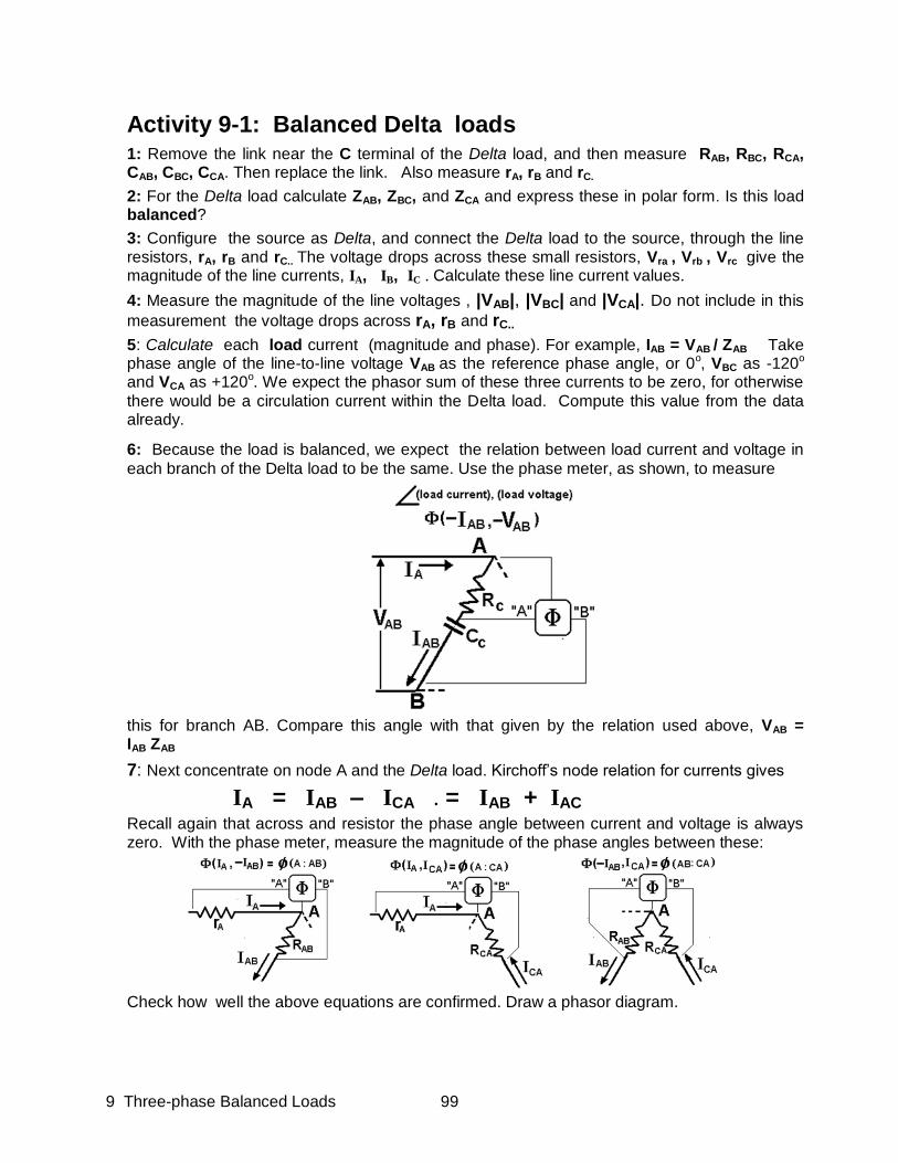
9 Three-phase Balanced Loads 99
Activity 9-1: Balanced Delta loads
1: Remove the link near the C terminal of the Delta load, and then measure RAB, RBC, RCA, CAB, CBC, CCA. Then replace the link. Also measure rA, rB and rC.
2: For the Delta load calculate ZAB, ZBC, and ZCA and express these in polar form. Is this load balanced?
3: Configure the source as Delta, and connect the Delta load to the source, through the line resistors, rA, rB and rC.. The voltage drops across these small resistors, Vra , Vrb , Vrc give the magnitude of the line currents, IA, IB, IC . Calculate these line current values.
4: Measure the magnitude of the line voltages , |VAB|, |VBC| and |VCA|. Do not include in this
measurement the voltage drops across rA, rB and rC..
5: Calculate each load current (magnitude and phase). For example, IAB = VAB / ZAB Take phase angle of the line-to-line voltage VAB as the reference phase angle, or 0o, VBC as -120o and VCA as +120o. We expect the phasor sum of these three currents to be zero, for otherwise
there would be a circulation current within the Delta load. Compute this value from the data already.
6: Because the load is balanced, we expect the relation between load current and voltage in
each branch of the Delta load to be the same. Use the phase meter, as shown, to measure
this for branch AB. Compare this angle with that given by the relation used above, VAB = IAB ZAB
7: Next concentrate on node A and the Delta load. Kirchoff’s node relation for currents gives
IA = IAB – ICA . = IAB + IAC
Recall again that across and resistor the phase angle between current and voltage is always zero. With the phase meter, measure the magnitude of the phase angles between these:
Check how well the above equations are confirmed. Draw a phasor diagram.
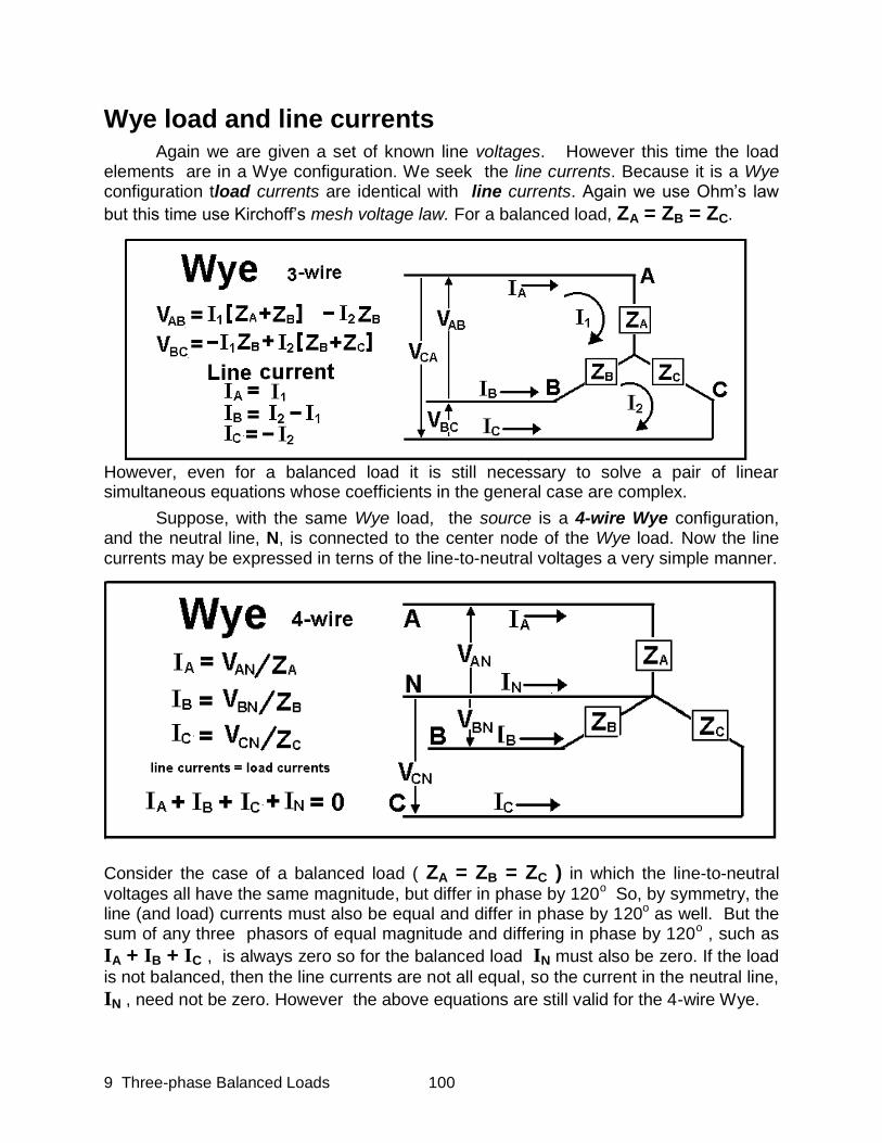
9 Three-phase Balanced Loads 100
Wye load and line currents
Again we are given a set of known line voltages. However this time the load elements are in a Wye configuration. We seek the line currents. Because it is a Wye configuration tload currents are identical with line currents. Again we use Ohm’s law
but this time use Kirchoff’s mesh voltage law. For a balanced load, ZA = ZB = ZC.
However, even for a balanced load it is still necessary to solve a pair of linear simultaneous equations whose coefficients in the general case are complex.
Suppose, with the same Wye load, the source is a 4-wire Wye configuration, and the neutral line, N, is connected to the center node of the Wye load. Now the line currents may be expressed in terns of the line-to-neutral voltages a very simple manner.
Consider the case of a balanced load ( ZA = ZB = ZC ) in which the line-to-neutral
voltages all have the same magnitude, but differ in phase by 120o So, by symmetry, the line (and load) currents must also be equal and differ in phase by 120o as well. But the sum of any three phasors of equal magnitude and differing in phase by 120o , such as
IA + IB + IC , is always zero so for the balanced load IN must also be zero. If the load
is not balanced, then the line currents are not all equal, so the current in the neutral line,
IN , need not be zero. However the above equations are still valid for the 4-wire Wye.

9 Three-phase Balanced Loads 101
Activity 9-2: Balanced Wye loads
1: Measure the Wye load values of RA, RB, RC, CA, CB, CC. From these values, compute ZA , ZB , ZC . Is the load balanced?
2: Also measure rA, rb and rc. and then connect the Wye load to the Wye source, through
the resistors ra, rb and rc..
3: Measure the three line-to-neutral voltages, |VAN|, |VBN| and |VCN| and assume their corresponding phase angle to be 0o, –120o and +120o. From this data compute the
magnitude and phase of the line cirrents, IA , IB and IC, using the equations displayed in
the 4-wire Wye box above. Find the sum of these three line currents.
4: Measure Vra , Vrb and Vrc , the voltages across ra, rb and rc. and from this data
compute the magnitude of the line currents, |IA| , |IB| and |IC|. Compare these with the
results of step 3. If the load is balanced, do the line currents all have the same magnitude?
5: Connect the phase meter to line A as shown in the diagram above and measure the angle between IA and VAN and compare this with the results found in step 3.
6: Disconnect the neutral line, and then measure the voltage between the common point of the Wye source and the Wye load. In theory this should be zero if the load is balanced.
7: Place a jumper across the capacitor in the C branch of the Wye load, so the load is no
longer balanced. Repeat step 6 for this configuration.

9 Three-phase Balanced Loads 102
S = ZAB + ZBC + ZCA
ZYA = ZAB ZCA / S
ZYB = ZAB ZC / S
ZYC = ZCA ZBC / S
SS = ZYAZYB + ZYBZYC + ZYCZYA
ZAB = SS/ZYC
ZBC = SS/ZYA
ZCA = SS /ZYB
Wye-Delta Transformations Wye-Delta transformations were
discussed in Electric Circuits I. The
equations derived there involve purely resistive load elements. For transformations of reactive load elements, the derivation and end results are similar, so we may borrow those
equations, changing only R to Z. If a Delta load is replaced by a Wye load with components given by these equations, the resulting line currents will be identical The two circuits are said to be equivalent. In analyzing Delta configurations it is sometimes useful to transform the load from Delta to Wye to simplify calculations.
Single-phase Power
Activity 9-3 Wye-Delta transformations
The Wye and Delta loads on the module, when all capacitors are by-passed, are approximately electrically equivalent, that is, the line currents are the same for either load.
1 Measure RA , RB and RC of the Wye load. By-pass the three capacitors. Then ZYA = RA, ZYB = RB, ZYC = RC.
2: From the transformation equations, calculate ZAB , ZBC and ZCA . Since the Wye
values are all real, the Delta values should also be real. Measure the values of three Delta resistors, RAB, RBC , RCA . With the capacitors of the Delta load by-passed, are these two loads equivalent, that is, do they satisfy the transformation equations?
3: Measure the three resistors, ra , rb , rc
4: Connect the Wye source to the Wye load (without capacitors) through the three r resistors
and measure the magnitude of the three line currents, |IA|, |IB|, |IC| (voltage across r
divided by r )
5: Repeat step 4 but use the Delta load. Are the line currents approximately the same for
the two configurations?

9 Three-phase Balanced Loads 103
Total power for a balanced load
To apply Eq (1), note that the same is used for each phase, since this depends on the nature of the balanced load. However the timing of the phases
differ by one-third period, or T/3. So replace 2t by
2t+ nT/3) where n = 0,1,2. Recall that = 2/T:
2t+ nT/3 ) = 2t + 2 (2/T) (nT/3)
= 2t + 4n/3 = 2t + n x 240o
Therefore Ptotal (t) = PA(t) + PB(t) + PC(t)
= 3 Vrms Irms cos +
+ Vrms Irms [ cos(t) + cos(t + 240o)
+ cos(t + 480o) ] .
For phase angles, +240o = –120o and +480o = 360o + 120o = +120o. So the expression within the square brackets is just the sum of three phasors of equal magnitude differing in phase by 120o, which is always zero, as already seen. So the instantaneous
total power, Ptotal (t), is actually independent of time!
In a single-phase circuit with constant source voltage and load impedance, the
instantaneous power, P(t), is constant . If the source voltage is sinusoidal, Vw cos t, then even with a constant load the instantaneous power, P(t), varies with time. For an
arbitrary load, let be the phase difference between voltage and current. Then
P(t) = [Vm cos t] [ Im cos (t + ) ]
This expression may be transformed using Eq. 11 of Notes on Trigonometry and the
peak vs root-mean-square relation, Irms = Im / √2
If the load is purely resistive so = 0 and cos = 1, then P(t) is never negative
and varies between 0 and 2 VrmsIrms . If the load has also a reactive component, so
≠ 0 and 0 ≤ cos < 1 then P(t) will be negative twice each cycle, that is energy is returned from the load to the power source, the so-called reactive power.
Three-phase Power
The three separate transformers or generator coils, connected either as Wye or Delta, individually act as single-phase systems. If the three-phase load is balanced, either Wye or Delta, each source must provide just one-third the total power because of the symmetry of the circuit. The surprising result is that for any balanced load the total instantaneous power, Ptotal (t) =
3 Vrms Irms cos does not vary with time even though each phase’s contribution does change with time, as given by Eq. (1). This constant Ptotal is never negative. A negative value would indicate a constant flow of power from the load back to the source, an impossible situation.
P(t) = Vrms Irms [ cos + cos ( 2t + ) ] (1)

9 Three-phase Balanced Loads 104
Note that the in Eq. (2) is the angle between the phase current and phase
voltage.
The torque of an electric motor at any moment is proportional to the supplied power. For a single-phase motor twice each cycle the supplied power is zero. Three-phase motors are balanced loads, so the constant supplied power provides a constant torque.
In the above activity, terminals of the phase-meter were connected at points
“inside” the source and load. In practical measurements such connections may be inconvenient or even impossible. An alternate approach is to connect watt-meters between the source and load and sum their individual readings..
P(t) = 3 Vrms Irms cos [for balanced 3-phase load] (2)
Activity 9-4 Verify P(t) = 3 Vrms Irms cos
1: Connect the source in the Wye 4-wire configuration.
2: Measure value of each resistance, RA , RB , RC of the Wye load. Then connect this Wye
load to the source, and include the capacitor in each branch, as shown in the diagram above.
3: Measure the voltage, VR , across each load resistor. Use the relation, Power = V2/R to
find the power dissipated by each load resistor. Add these to obtain total power, Ptotal . Also
use Ohm;s law to find each load current. and calculate their average, I.
4: Measure the phase voltage, Va’n .
5: Connect the phase meter, as shown, and measure the angle between the phase voltage
and the phase current (for Wye, phase and line currents equal)
6: Compare the predicted power value, 3 Va’n I cos , with Ptotal
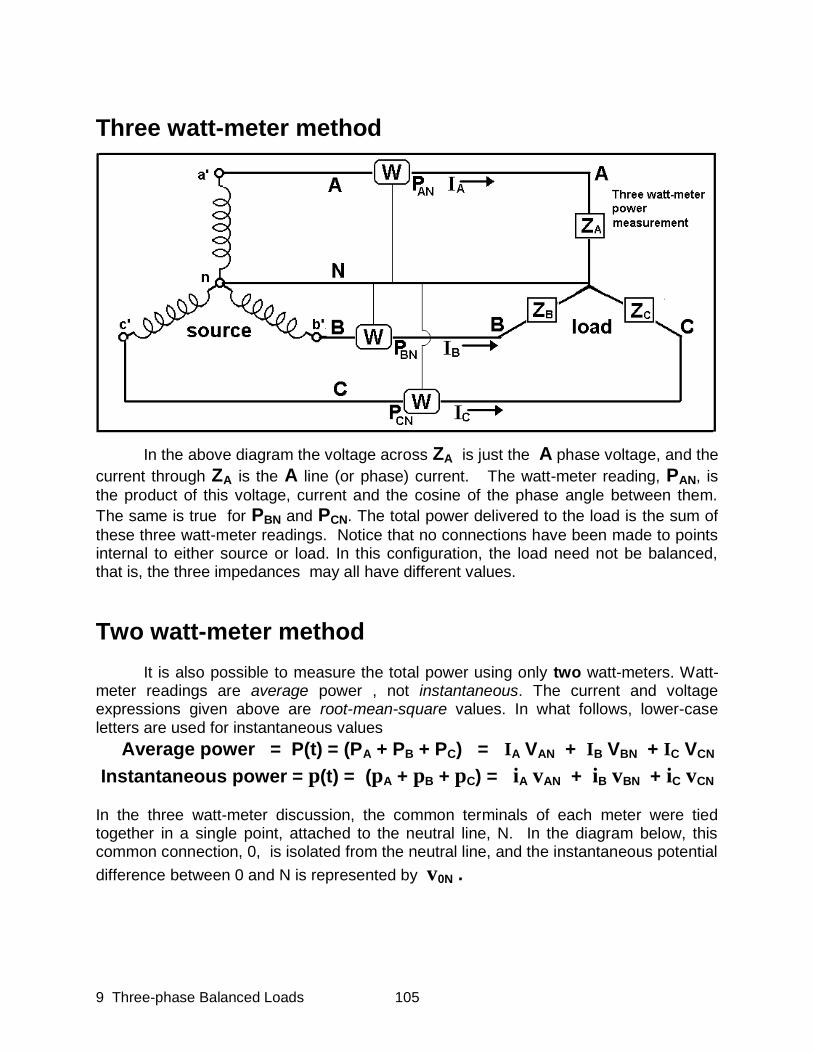
9 Three-phase Balanced Loads 105
Three watt-meter method
In the above diagram the voltage across ZA is just the A phase voltage, and the
current through ZA is the A line (or phase) current. The watt-meter reading, PAN, is
the product of this voltage, current and the cosine of the phase angle between them.
The same is true for PBN and PCN. The total power delivered to the load is the sum of
these three watt-meter readings. Notice that no connections have been made to points internal to either source or load. In this configuration, the load need not be balanced, that is, the three impedances may all have different values.
Two watt-meter method It is also possible to measure the total power using only two watt-meters. Watt-meter readings are average power , not instantaneous. The current and voltage expressions given above are root-mean-square values. In what follows, lower-case letters are used for instantaneous values
Average power = P(t) = (PA + PB + PC) = IA VAN + IB VBN + IC VCN
Instantaneous power = p(t) = (pA + pB + pC) = iA vAN + iB vBN + iC vCN
In the three watt-meter discussion, the common terminals of each meter were tied together in a single point, attached to the neutral line, N. In the diagram below, this common connection, 0, is isolated from the neutral line, and the instantaneous potential
difference between 0 and N is represented by v0N .
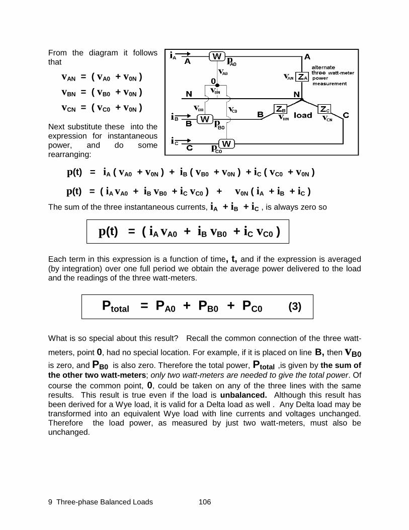
9 Three-phase Balanced Loads 106
From the diagram it follows that
vAN = ( vA0 + v0N )
vBN = ( vB0 + v0N )
vCN = ( vC0 + v0N ) Next substitute these into the expression for instantaneous power, and do some rearranging:
p(t) = iA ( vA0 + v0N ) + iB ( vB0 + v0N ) + iC ( vC0 + v0N )
p(t) = ( iA vA0 + iB vB0 + iC vC0 ) + v0N ( iA + iB + iC )
The sum of the three instantaneous currents, iA + iB + iC , is always zero so
Each term in this expression is a function of time, t, and if the expression is averaged
(by integration) over one full period we obtain the average power delivered to the load and the readings of the three watt-meters.
What is so special about this result? Recall the common connection of the three watt-
meters, point 0, had no special location. For example, if it is placed on line B, then vB0
is zero, and PB0 is also zero. Therefore the total power, Ptotal ,is given by the sum of
the other two watt-meters; only two watt-meters are needed to give the total power. Of
course the common point, 0, could be taken on any of the three lines with the same results. This result is true even if the load is unbalanced. Although this result has been derived for a Wye load, it is valid for a Delta load as well . Any Delta load may be transformed into an equivalent Wye load with line currents and voltages unchanged. Therefore the load power, as measured by just two watt-meters, must also be unchanged.
p(t) = ( iA vA0 + iB vB0 + iC vC0 )
Ptotal = PA0 + PB0 + PC0 (3)
9 Three-phase Balanced Loads 107
In a single-phase circuit with a reactive load, the magnitude of the phase angle
between current and voltage never exceeds 90o , so average power, V cos , is
never negative. In three-phase systems, the phase angle may exceed 90o so a watt-meter reading for a given phase may be negative, although the sum of all readings ( two or three ) may never be negative.
Activity 9-5: Watt-meter measurements
1: Measure the values of the three Wye load resistors, RA , RB and RC
2: Configure the module board as a 4-wire Wye source and load. By-pass the three source
resistors, rA , rB and rC but include the capacitors in the Wye load.
3: Measure the voltage across RA and record this as VRA . Repeat for RB and RC . For each
of these resistors compute the power consumed, PAN = VRA2/ RA , etc.. and compute their
sum, the total load power..
4: Use the three watt-meter method to measure the power provided by each phase, PAN , PBN and PCN , and compute their sum.
5: Use the two watt-meter method to measure the power provided by each phase. Alternately
connect the watt-meters common point to lines A, B and C. For each choice of common point compute the sum of the two readings to obtain total power. How close to each other are these readings?
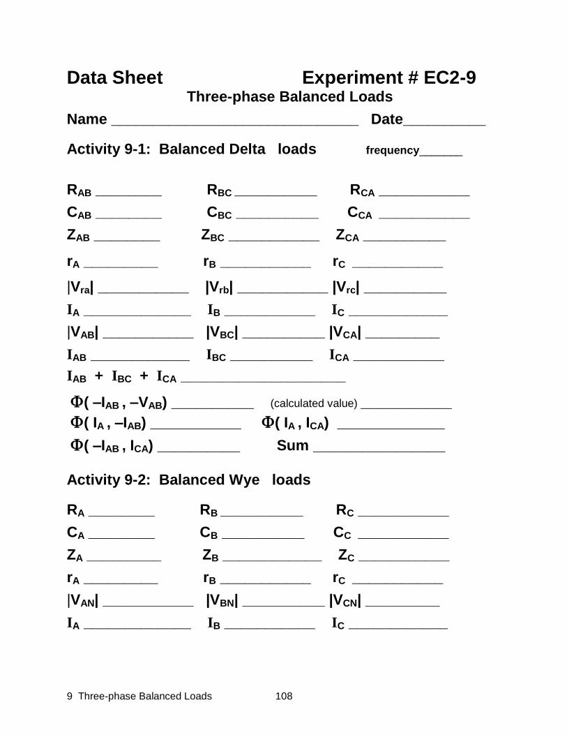
9 Three-phase Balanced Loads 108
Data Sheet Experiment # EC2-9 Three-phase Balanced Loads
Name ______________________________ Date__________
Activity 9-1: Balanced Delta loads frequency_______
RAB ________ RBC __________ RCA ___________
CAB ________ CBC __________ CCA ___________
ZAB ________ ZBC ___________ ZCA __________
rA _________ rB ___________ rC ___________
|Vra| ___________ |Vrb| ___________ |Vrc| __________
IA _____________ IB ___________ IC ____________
|VAB| ___________ |VBC| __________ |VCA| _________
IAB ____________ IBC __________ ICA ___________
IAB + IBC + ICA ____________________
( –IAB , –VAB) __________ (calculated value) ___________
( IA , –IAB) ___________ ( IA , ICA) _____________
( –IAB , ICA) __________ Sum ________________ Activity 9-2: Balanced Wye loads
RA ________ RB __________ RC ___________
CA ________ CB __________ CC ___________
ZA _________ ZB ____________ ZC ___________
rA _________ rB ___________ rC ___________
|VAN| ___________ |VBN| __________ |VCN| _________
IA _____________ IB ___________ IC ____________

9 Three-phase Balanced Loads 109
Data Sheet Experiment # EC2-9, continued
|Vra| ___________ |Vrb| __________ |Vrc| __________
|IA| ____________ |IB| ___________ |IC| ___________
(IA , –VAN) ______
Balanced load : VN-N ______ Unbalanced load : VN-N ______
Activity 9-3: Wye-Delta Transformations
RA ________ RB __________ RC ___________
Calculated values for: ZAB _________ ZBC ____________ ZCA___________
Measured values for:
RAB _________ RBC _____________ RCA ___________
rA _________ rB ___________ rC ___________
|Vra| ___________ |Vrb| __________ |Vrc| __________
|IA|mA |IB|mA |IC|mA
Wye
Delta
Activity 9-4: Verify P(t) = 3 Vrms Irms cos
RA _________ RB _________ RC __________
VRA ________ VRB _________ VRC _________
IA = VRA/RA ______ IB = VRB/RB ______ IC = VRC RC _______
PA = VRA2/RA ______ PB = VRB
2/RB _____ PC = VRC
2/ RC ______
I = I average _______ Ptotal ______ Va’n ______ _______
3 Va’n I cos _______
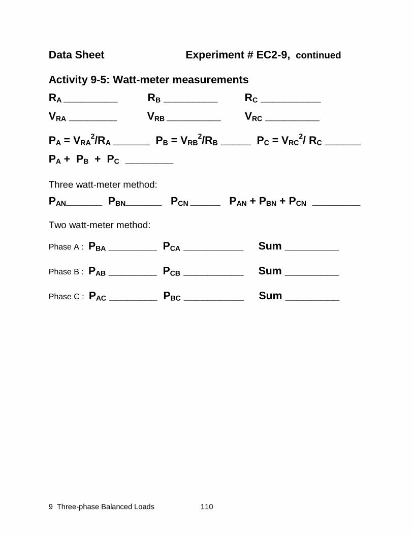
9 Three-phase Balanced Loads 110
Data Sheet Experiment # EC2-9, continued
Activity 9-5: Watt-meter measurements
RA _________ RB _________ RC __________
VRA ________ VRB _________ VRC _________
PA = VRA2/RA ______ PB = VRB
2/RB _____ PC = VRC
2/ RC ______
PA + PB + PC ________
Three watt-meter method:
PAN______ PBN______ PCN _____ PAN + PBN + PCN ________ Two watt-meter method:
Phase A : PBA ________ PCA __________ Sum _________ Phase B : PAB ________ PCB __________ Sum _________ Phase C : PAC ________ PBC __________ Sum _________

9 Three-phase Balanced Loads 111

10 Three-phase Unbalanced Loads 112
Three-phase Unbalanced Loads
Equipment: Function Generator, Phase Meter. Wattmeter, Oscilloscope
The previous experiment considered three-phase balanced loads, examining the line and load currents and power distribution. Because the load was balanced, the line currents were all equal and 120o out of phase with each other. Power distribution and load currents were also symmetrical. In the present experiment we explore unbalanced loads. We expect the line and load currents to differ, phase by phase. However, the basic equations for Delta and Wye loads (three-wire of 4-wire) presented in the previous experiment are still valid, although their application requires more involved calculations. Finding load currents involve complex division; line currents involve complex subtraction. The short stand-alone computer program, COMPLEX.EXE, is provided to facilitate such calculations. As before we assume the three-phase source to have balanced output voltages, and 120o phase differences
Unbalanced Delta loads
The Delta diagram of the previous experiment is reproduced here.
The three branches of the model Delta load are approximately equal. The diagram below suggests three possible methods for changing the capacitance of the CA branch.
ELECTRIC CIRCUITS II EC2-10
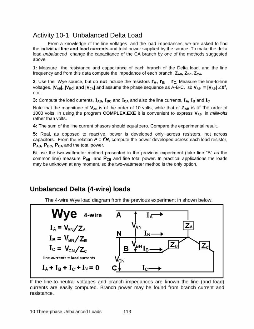
10 Three-phase Unbalanced Loads 113
Unbalanced Delta (4-wire) loads
The 4-wire Wye load diagram from the previous experiment in shown below.
If the line-to-neutral voltages and branch impedances are known the line (and load) currents are easily computed. Branch power may be found from branch current and resistance.
Activity 10-1 Unbalanced Delta Load
From a knowledge of the line voltages and the load impedances, we are asked to find the individual line and load currents and total power supplied by the source. To make the delta load unbalanced change the capacitance of the CA branch by one of the methods suggested
above
1: Measure the resistance and capacitance of each branch of the Delta load, and the line frequency and from this data compute the impedance of each branch, ZAB, ZBC, ZCA.
2: Use the Wye source, but do not include the resistors rA, rB , rC. Measure the line-to-line
voltages, |VAB|, |VBC| and |VCA| and assume the phase sequence as A-B-C, so VAB = |VAB| 0o,
etc..
3: Compute the load currents, IAB, IBC and ICA and also the line currents, IA, IB and IC
Note that the magnitude of VAB is of the order of 10 volts, while that of ZAB is of the order of
1000 volts. In using the program COMPLEX.EXE it is convenient to express VAB in millivolts rather than volts.
4: The sum of the line current phasors should equal zero. Compare the experimental result.
5: Real, as opposed to reactive, power is developed only across resistors, not across
capacitors. From the relation P = I2R, compute the power developed across each load resistor,
PAB, PBC, PCA and the total power.
6: use the two-wattmeter method presented in the previous experiment (take line “B” as the
common line) measure PAB and PCB and fine total power. In practical applications the loads
may be unknown at any moment, so the two-wattmeter method is the only option.
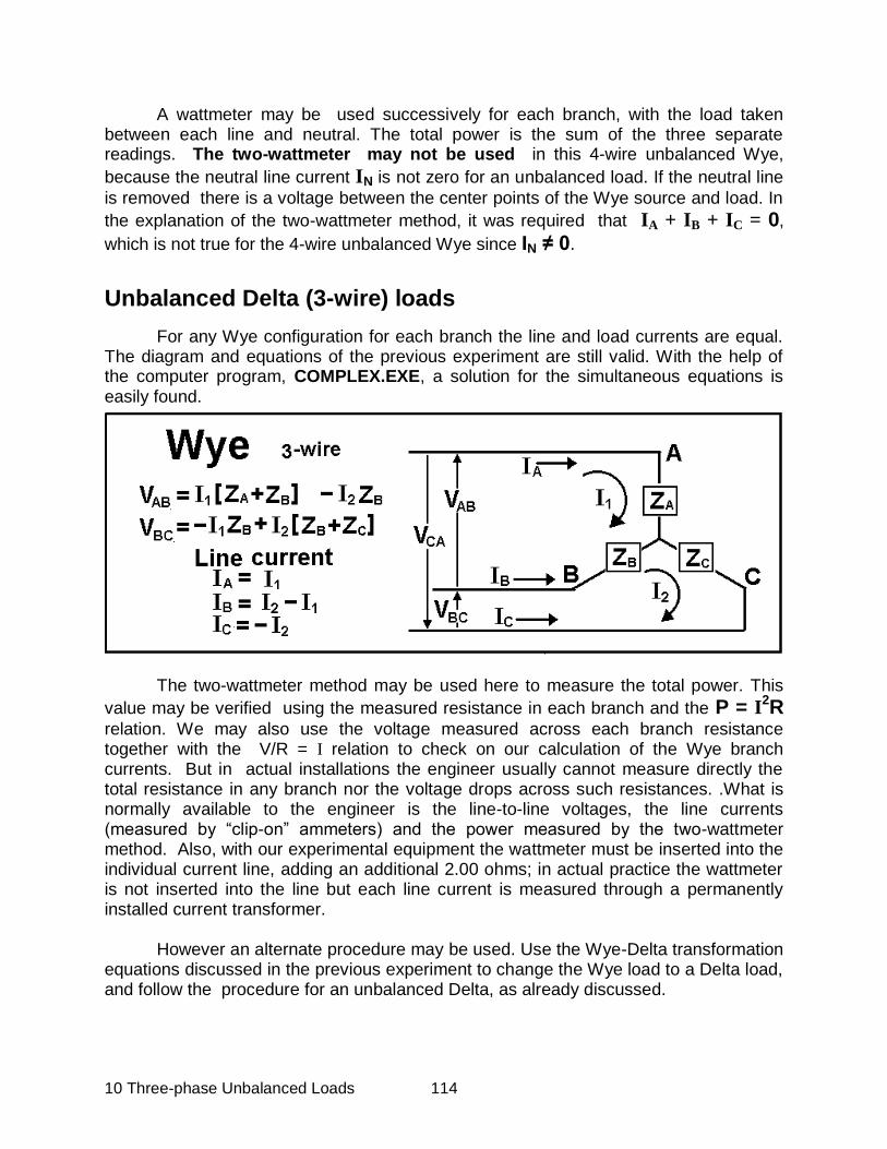
10 Three-phase Unbalanced Loads 114
A wattmeter may be used successively for each branch, with the load taken between each line and neutral. The total power is the sum of the three separate readings. The two-wattmeter may not be used in this 4-wire unbalanced Wye,
because the neutral line current IN is not zero for an unbalanced load. If the neutral line
is removed there is a voltage between the center points of the Wye source and load. In
the explanation of the two-wattmeter method, it was required that IA + IB + IC = 0,
which is not true for the 4-wire unbalanced Wye since IN ≠ 0.
Unbalanced Delta (3-wire) loads
For any Wye configuration for each branch the line and load currents are equal. The diagram and equations of the previous experiment are still valid. With the help of the computer program, COMPLEX.EXE, a solution for the simultaneous equations is easily found.
The two-wattmeter method may be used here to measure the total power. This
value may be verified using the measured resistance in each branch and the P = I2R
relation. We may also use the voltage measured across each branch resistance together with the V/R = I relation to check on our calculation of the Wye branch currents. But in actual installations the engineer usually cannot measure directly the total resistance in any branch nor the voltage drops across such resistances. .What is normally available to the engineer is the line-to-line voltages, the line currents (measured by “clip-on” ammeters) and the power measured by the two-wattmeter method. Also, with our experimental equipment the wattmeter must be inserted into the individual current line, adding an additional 2.00 ohms; in actual practice the wattmeter is not inserted into the line but each line current is measured through a permanently installed current transformer. However an alternate procedure may be used. Use the Wye-Delta transformation equations discussed in the previous experiment to change the Wye load to a Delta load, and follow the procedure for an unbalanced Delta, as already discussed.

10 Three-phase Unbalanced Loads 115
Activity 10-2 Unbalanced Wye Load
1: Change the capacitance of the C branch of the Wye load by adding a capacitor, CX, in
parallel with CC
2: Measure the R and C values for each branch of the Wye load, and also the line
frequency. .From this data calculate the branch impedances, ZA, ZB, ZC
3: Connect the Wye load directly to the Wye source, bypassing resistors rA, rB, rC. Do not use
the neutral line.
4: Measure the line-to-line voltages, |VAB|, |VBC| and |VCA| and assume the phase
sequence as A-B-C, so VAB =| VAB| 0o, etc..
Power calculations
5: Use the two-wattmeter method to determine total power. Make three trials, using different
lines as “common”.
6: As a check on the two-wattmeter method, measure the voltage drop across the three
branch resistors, VRa, VRb, VRc, and from this calculate the power dissipated in each
branch using the relation P = V2/R. Add these to obtain total load power.
Neutral-to-neutral voltage
7: In a 4-wire balanced system, there is no current in the neutral line. Even without this line
no voltage difference exists between the common points of the Wye source and load. This is not the case for unbalances Wye loads. Measure this voltage difference for the present setup.
Line currents by simultaneous equations
8: Use the notation of the Wye 3-wire diagram and calculate the loop currents, I1, I2 and
also the three line currents, IA, IB , IC . When using the computer program,
COMPLEX.EXE express voltages in millivolts whenever necessary to improve precision.
9: As a check on the above results calculate the line currents using the voltage drop across
each branch resistor (not the line-to-line voltage!) and Ohm’s law
Line currents by Wye-Delta transformation
10 Transform the Wye load to a Delta, using COMPLEX.EXE, to obtain values for , ZAB, ZBC, ZCA. Then use the procedure of Activity 13-1 to get the Delta branch currents , IAB, IBC and ICA and also the line currents, IA, IB and IC . Do the Wye-Delta transformation and the
simultaneous equation method give comparable results for the line currents?
11: For a comparison, calculate the magnitude of the line currents by Ohm’s law, as
|IA| = VRa/RA etc..
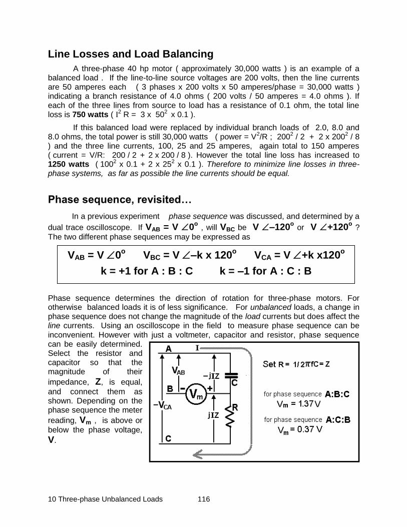
10 Three-phase Unbalanced Loads 116
Line Losses and Load Balancing
A three-phase 40 hp motor ( approximately 30,000 watts ) is an example of a balanced load . If the line-to-line source voltages are 200 volts, then the line currents are 50 amperes each ( 3 phases x 200 volts x 50 amperes/phase = 30,000 watts ) indicating a branch resistance of 4.0 ohms ( 200 volts / 50 amperes = 4.0 ohms ). If each of the three lines from source to load has a resistance of 0.1 ohm, the total line loss is 750 watts ( I2 R = 3 x 502 x 0.1 ).
If this balanced load were replaced by individual branch loads of 2.0, 8.0 and 8.0 ohms, the total power is still 30,000 watts ( power = V2/R ; 2002 / 2 + 2 x 2002 / 8 ) and the three line currents, 100, 25 and 25 amperes, again total to 150 amperes ( current = V/R: 200 / 2 + 2 x 200 / 8 ). However the total line loss has increased to 1250 watts ( 1002 x 0.1 + 2 x 252 x 0.1 ). Therefore to minimize line losses in three-phase systems, as far as possible the line currents should be equal.
Phase sequence, revisited…
In a previous experiment phase sequence was discussed, and determined by a
dual trace oscilloscope. If VAB = V 0o , will VBC be V –120
o or V +120
o ?
The two different phase sequences may be expressed as
Phase sequence determines the direction of rotation for three-phase motors. For otherwise balanced loads it is of less significance. For unbalanced loads, a change in phase sequence does not change the magnitude of the load currents but does affect the line currents. Using an oscilloscope in the field to measure phase sequence can be inconvenient. However with just a voltmeter, capacitor and resistor, phase sequence can be easily determined. Select the resistor and capacitor so that the magnitude of their
impedance, Z, is equal,
and connect them as shown. Depending on the phase sequence the meter
reading, Vm , is above or
below the phase voltage,
V.
VAB = V 0o VBC = V –k x 120
o VCA = V +k x120
o
k = +1 for A : B : C k = –1 for A : C : B
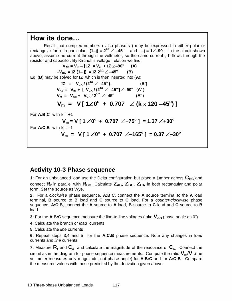
10 Three-phase Unbalanced Loads 117
How its done…
Recall that complex numbers ( also phasors ) may be expressed in either polar or
rectangular form. In particular, (1–j) = 21/2 –45o and –j = 1–90o . In the circuit shown above, assume no current through the voltmeter, so the same current , I, flows through the resistor and capacitor. By Kirchoff’s voltage relation we find:
VAB = Vm – j IZ = Vm + IZ –90o (A)
–VCA = IZ (1– j) = IZ 21/2 –45o (B)
Eq. (B) may be solved for IZ which is then inserted into (A):
IZ = –VCA / (21/2 –45o ) (B’)
VAB = Vm + [–VCA / (21/2 –45o)] –90o (A’ )
Vm = VAB + VCA / 21/2 –45o (A”)
Vm = V [ 10o + 0.707 (k x 120 –45
o) ]
For A:B:C with k = +1
Vm = V [ 1 0o + 0.707 +75
o ] = 1.37 +30
o
For A:C:B with k = –1
Vm = V [ 1 0o + 0.707 –165
o ] = 0.37 –30
o
Activity 10-3 Phase sequence
1: For an unbalanced load use the Delta configuration but place a jumper across CBC and
connect Rr in parallel with RBC. Calculate ZAB, ZBC, ZCA in both rectangular and polar
form. Set the source as Wye.
2: For a clockwise phase sequence, A:B:C, connect the A source terminal to the A load terminal, B source to B load and C source to C load. For a counter-clockwise phase sequence, A:C:B, connect the A source to A load, B source to C load and C source to B
load.
3: For the A:B:C sequence measure the line-to-line voltages (take VAB phase angle as 0o)
4: Calculate the branch or load currents
5: Calculate the line currents
6: Repeat steps 3,4 and 5 for the A:C:B phase sequence. Note any changes in load currents and line currents.
7: Measure Rr and Cx and calculate the magnitude of the reactance of Cx. Connect the
circuit as in the diagram for phase sequence measurements. Compute the ratio Vm/V .(the
voltmeter measures only magnitude, not phase angle) for A:B:C and for A:C:B . Compare
the measured values with those predicted by the derivation given above.
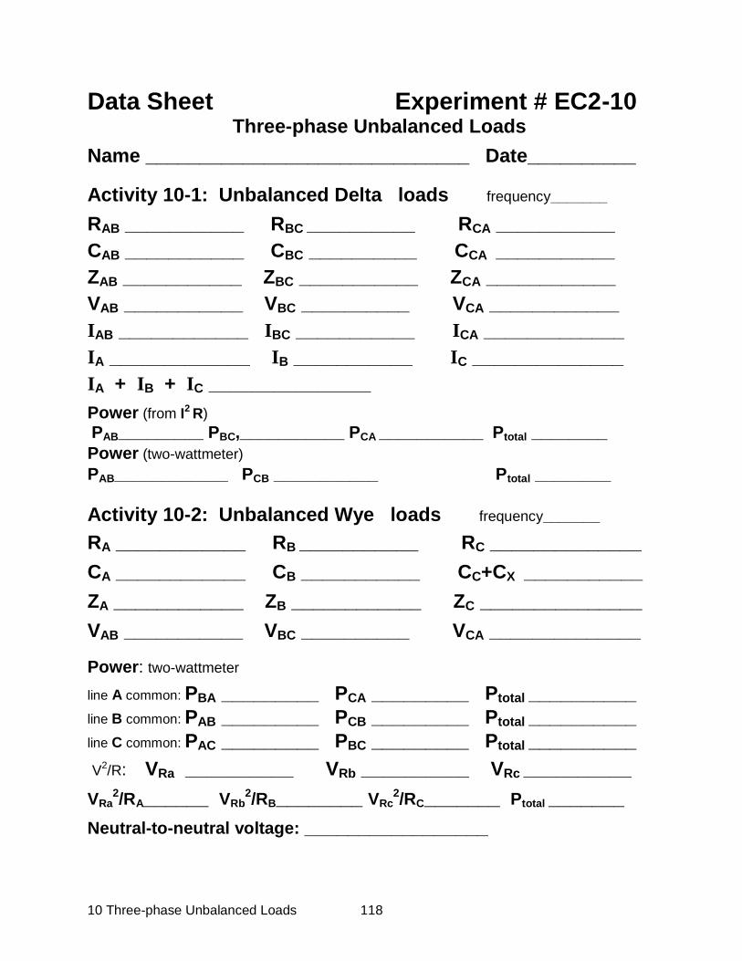
10 Three-phase Unbalanced Loads 118
Data Sheet Experiment # EC2-10
Three-phase Unbalanced Loads
Name ______________________________ Date__________
Activity 10-1: Unbalanced Delta loads frequency_______
RAB ___________ RBC __________ RCA ___________
CAB ___________ CBC __________ CCA ___________
ZAB ___________ ZBC ___________ ZCA ____________
VAB ___________ VBC __________ VCA ____________
IAB ____________ IBC ___________ ICA _____________
IA _____________ IB ___________ IC ______________
IA + IB + IC _______________
Power (from I2 R)
PAB_________ PBC,___________ PCA ___________ Ptotal ________
Power (two-wattmeter)
PAB____________ PCB ___________ Ptotal ________
Activity 10-2: Unbalanced Wye loads frequency_______
RA ____________ RB ___________ RC ______________
CA ____________ CB ___________ CC+CX ___________
ZA ____________ ZB ____________ ZC _______________
VAB ___________ VBC __________ VCA ______________
Power: two-wattmeter
line A common: PBA _________ PCA _________ Ptotal __________
line B common: PAB _________ PCB _________ Ptotal __________
line C common: PAC _________ PBC _________ Ptotal __________
V2/R: VRa __________ VRb __________ VRc __________
VRa2/RA______ VRb
2/RB________ VRc
2/RC_______ Ptotal _______
Neutral-to-neutral voltage: _________________
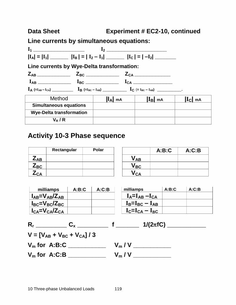
10 Three-phase Unbalanced Loads 119
Rectangular Polar
ZAB
ZBC
ZCA
A:B:C A:C:B
VAB VBC
VCA
milliamps A:B:C A:C:B
IAB=VAB/ZAB
IBC=VBC/ZBC
ICA=VCA/ZCA
milliamps A:B:C A:C:B
IA=IAB –ICA
IB=IBC – IAB
IC=ICA – IBC
Data Sheet Experiment # EC2-10, continued
Line currents by simultaneous equations:
I1 _________________ I2 ____________________
|IA| = |I1| ______ |IB | = | I2 – I1| ______ |IC | = | –I2| _______
Line currents by Wye-Delta transformation:
ZAB ___________ ZBC ___________ ZCA ____________
IAB ___________ IBC ___________ ICA _____________
IA (=IAB – ICA) _______ IB (=IBC – IAB) ________ IC (= IBC – IAB) ________.
Method |IA| mA |IB| mA |IC| mA Simultaneous equations
Wye-Delta transformation VR / R
Activity 10-3 Phase sequence
Rr ________ Cx ________ f ______ 1/(2fC) __________
V = [VAB + VBC + VCA] / 3
Vm for A:B:C ___________ Vm / V ___________
Vm for A:C:B ___________ Vm / V ___________
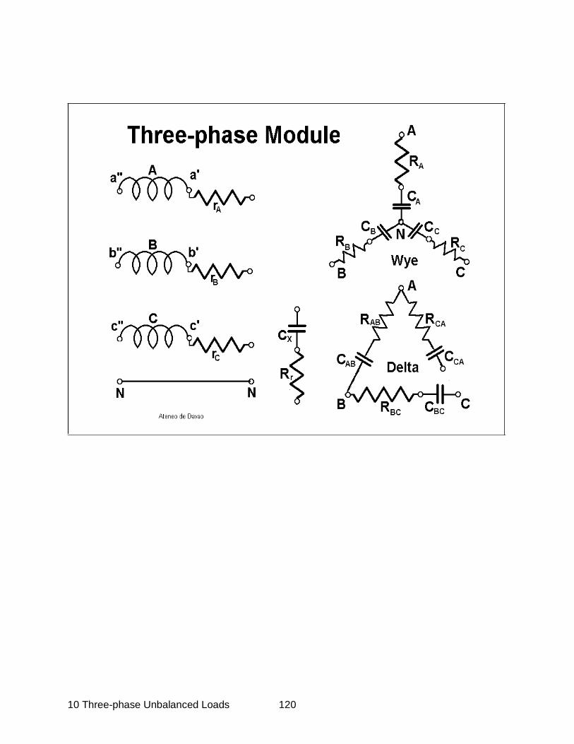
10 Three-phase Unbalanced Loads 120
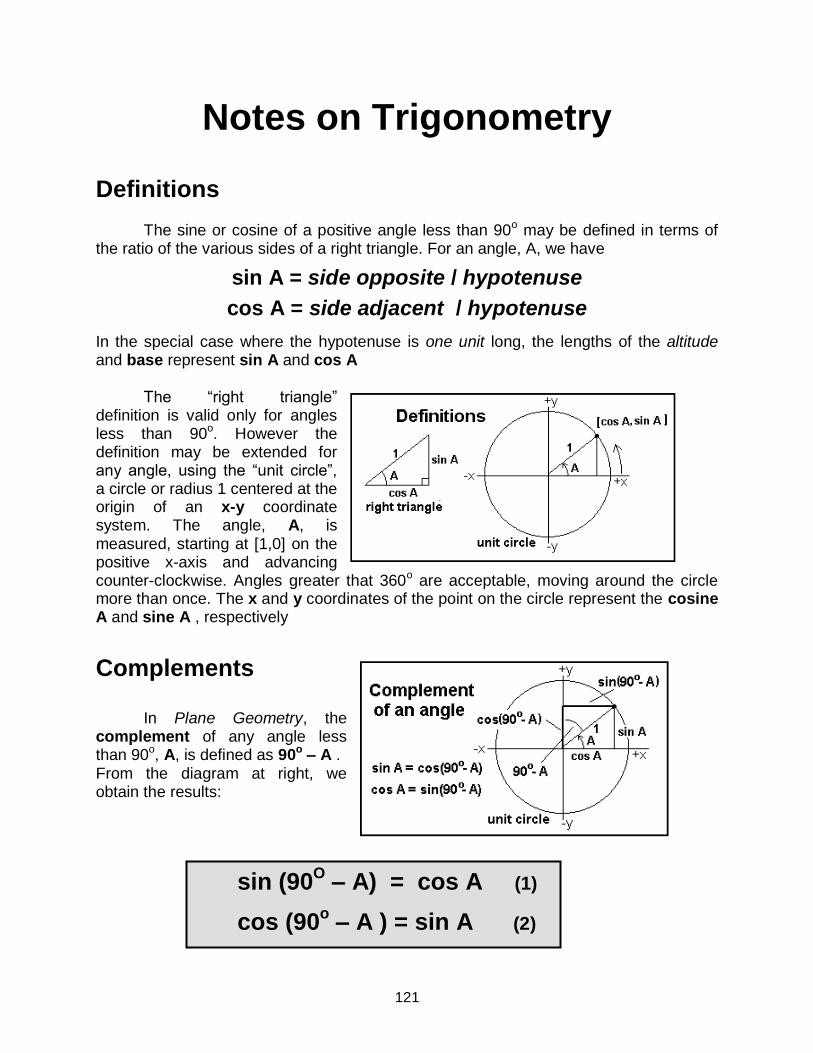
121
Notes on Trigonometry
Definitions The sine or cosine of a positive angle less than 90o may be defined in terms of the ratio of the various sides of a right triangle. For an angle, A, we have
sin A = side opposite / hypotenuse
cos A = side adjacent / hypotenuse
In the special case where the hypotenuse is one unit long, the lengths of the altitude and base represent sin A and cos A The “right triangle” definition is valid only for angles less than 90o. However the definition may be extended for any angle, using the “unit circle”, a circle or radius 1 centered at the origin of an x-y coordinate system. The angle, A, is measured, starting at [1,0] on the positive x-axis and advancing counter-clockwise. Angles greater that 360o are acceptable, moving around the circle more than once. The x and y coordinates of the point on the circle represent the cosine A and sine A , respectively
Complements In Plane Geometry, the complement of any angle less than 90o, A, is defined as 90o – A . From the diagram at right, we obtain the results:
sin (90O – A) = cos A (1)
cos (90o – A ) = sin A (2)

122
Supplements In Plane Geometry, the supplement of any angle less than 180o, A, is defined as 180o – A . From the diagram at right, we obtain the results:
Negative angles Negative angles are represented by moving clockwise from [1,0] on the unit circle diagram, as indicated in the diagram at right.
Sines and cosines of the sum of two angles
The sine of the sum of two angles does not equal the sum of the sines. The diagram below shows two representations of the angle (B – A). In each
case the distance, D, between the two points on the unit circle is the same.
sin (180o – A) = sin A (3)
cos (180o – A) = – cos A (4)
sin –A = – sin A (5)
cos –A = cos A (6)
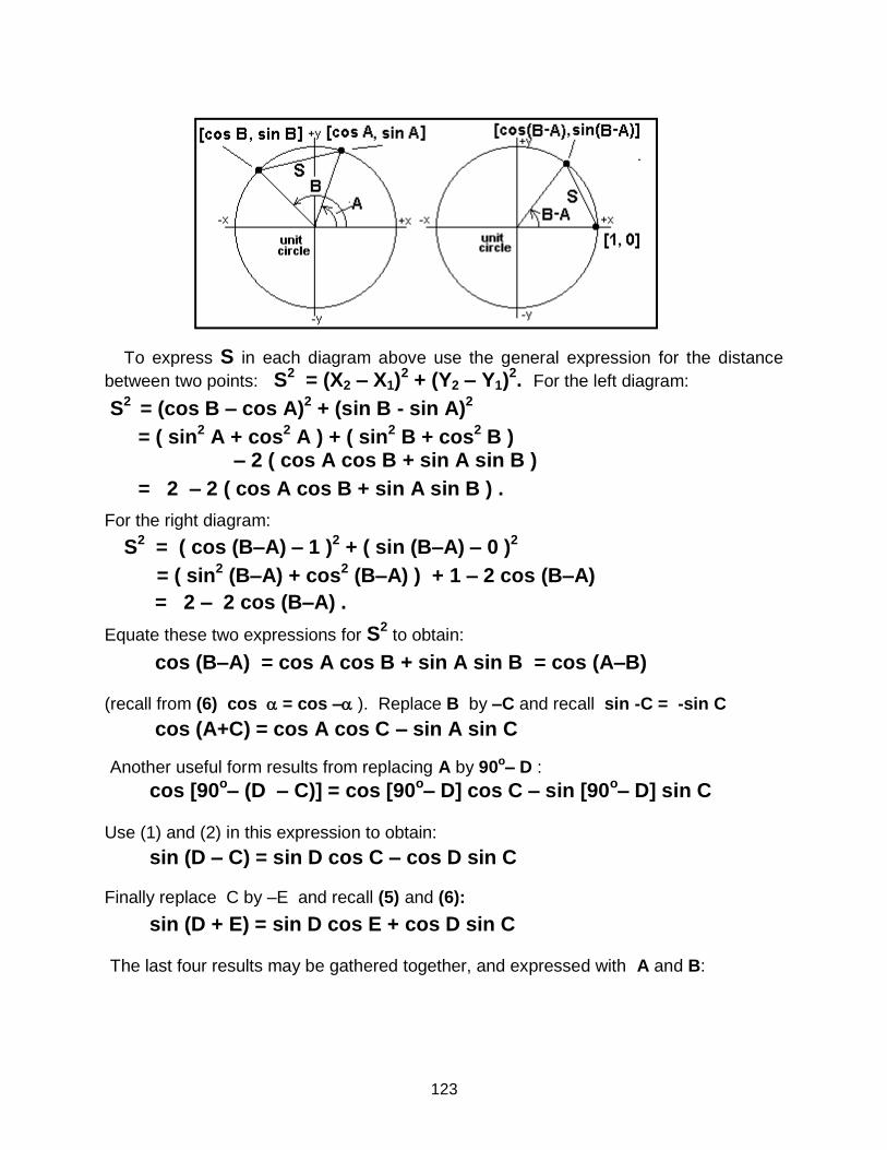
123
To express S in each diagram above use the general expression for the distance
between two points: S2 = (X2 – X1)
2 + (Y2 – Y1)
2. For the left diagram:
S2 = (cos B – cos A)
2 + (sin B - sin A)
2
= ( sin2 A + cos
2 A ) + ( sin
2 B + cos
2 B )
– 2 ( cos A cos B + sin A sin B )
= 2 – 2 ( cos A cos B + sin A sin B ) .
For the right diagram:
S2 = ( cos (B–A) – 1 )
2 + ( sin (B–A) – 0 )
2
= ( sin2 (B–A) + cos
2 (B–A) ) + 1 – 2 cos (B–A)
= 2 – 2 cos (B–A) .
Equate these two expressions for S2 to obtain:
cos (B–A) = cos A cos B + sin A sin B = cos (A–B)
(recall from (6) cos = cos – ). Replace B by –C and recall sin -C = -sin C
cos (A+C) = cos A cos C – sin A sin C
Another useful form results from replacing A by 90o– D :
cos [90o– (D – C)] = cos [90
o– D] cos C – sin [90
o– D] sin C
Use (1) and (2) in this expression to obtain:
sin (D – C) = sin D cos C – cos D sin C
Finally replace C by –E and recall (5) and (6):
sin (D + E) = sin D cos E + cos D sin C The last four results may be gathered together, and expressed with A and B:
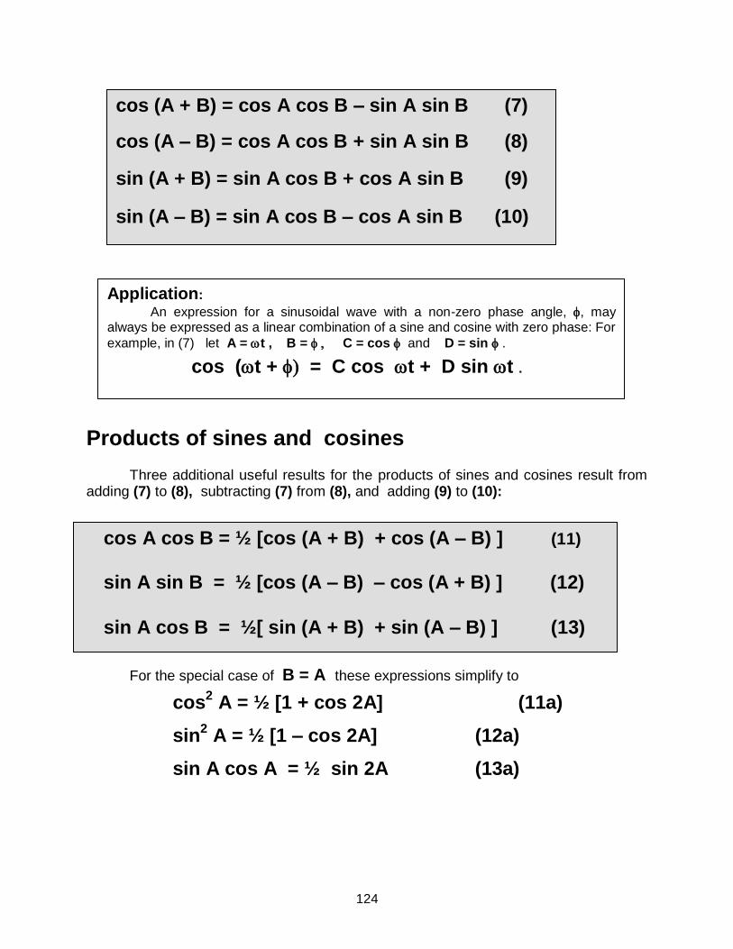
124
Products of sines and cosines Three additional useful results for the products of sines and cosines result from adding (7) to (8), subtracting (7) from (8), and adding (9) to (10):
For the special case of B = A these expressions simplify to
cos2 A = ½ [1 + cos 2A] (11a)
sin2 A = ½ [1 – cos 2A] (12a)
sin A cos A = ½ sin 2A (13a)
Application:
An expression for a sinusoidal wave with a non-zero phase angle, , may always be expressed as a linear combination of a sine and cosine with zero phase: For
example, in (7) let A = t , B = C = cos and D = sin .
cos (t + = C cos t + D sin t .
cos A cos B = ½ [cos (A + B) + cos (A – B) ] (11)
sin A sin B = ½ [cos (A – B) – cos (A + B) ] (12)
sin A cos B = ½[ sin (A + B) + sin (A – B) ] (13)
cos (A + B) = cos A cos B – sin A sin B (7)
cos (A – B) = cos A cos B + sin A sin B (8)
sin (A + B) = sin A cos B + cos A sin B (9)
sin (A – B) = sin A cos B – cos A sin B (10)

125
Sum of sines and cosines Expressions (7) to (10) involved the sine or cosine for the sum or difference of two angles. Here we consider the sum of the sines or cosines themselves. Use the following substitutions in (11) and (12) C = A + B and D = A – B or A = ½(C + D) and B = ½(C – D)
cos C + cos D = 2 cos ½(C + D) cos ½(C – D) (14)
sin C + sin D = 2 sin ½(C + D) cos ½(C – D) (15)
Application:
The sum of two waves of almost the same frequency produces a wave of
varying amplitude (beats). Let C = ( ) t and D = t and use (14):
cos t + cos ( ) t = [2 cos t ] cos ( ) t
126
Ateneo de Davao University
Electronic Communication Series
Electric Circuits I: Direct Current Electric Circuits II: Alternating Current Electronics I: Basic Components Electronics II: Amplifiers and Oscillators Electronics III: Operational Amplifiers Communications I: AM and FM Communications II: Digital Communications Digital Logic Circuits, with Verilog HDL Industrial Electronics LOGO! PLC: Learning a Programmable Logic Controller
We are a university in a Third World country, the Philippines. We believe that more than chalk and whiteboard pens are needed to train a communication engineer for today’s world. “Hands on” is a must for every student. Excellent student laboratory equipment is readily available on the world markets. Yet the funding necessary for us to purchase such equipment, and in the quantity we desired, was completely unavailable. Our only viable option was to design and fabricate locally the materials of which before we only dreamt. For each item of laboratory equipment student instructional material had to be prepared, as shown in the above listing. With a view to share with other institutions the fruit of our own endeavors, we are making these student manuals freely available. Permission is given to copy this material, and to suitably modify it to the needs of a particular institution.
Copyright © 2022 FDOKUMEN