Homotopic Object Reconstruction using NaturalNeighbor Barycentric Coordinates

Ojaswa Sharma1 and Francois Anton2

1 Department of Computer Science and Engineering,Indian Institute of Technology Bombay,

Mumbai, 400076, Indiaojaswa@cse.iitb.ac.in

2 Department of Informatics and Mathematical Modelling,Technical University of Denmark, Lyngby, 2800, Denmark

fa@imm.dtu.dk

Abstract. One of the challenging problems in computer vision is ob-ject reconstruction from cross sections. In this paper, we address theproblem of 2D object reconstruction from arbitrary linear cross sections.This problem has not been much discussed in the literature, but holdsgreat importance since it lifts the requirement of order within the crosssections in a reconstruction problem, consequently making the recon-struction problem harder. Our approach to the reconstruction is viacontinuous deformations of line intersections in the plane. We defineVoronoi diagram based barycentric coordinates on the edges of n-sidedconvex polygons as the area stolen by any point inside a polygon from theVoronoi regions of each open oriented line segment bounding the polygon.These allow us to formulate homotopies on edges of the polygons fromwhich the underlying object can be reconstructed. We provide results ofthe reconstruction including the necessary derivation of the gradient atpolygon edges and the optimal placement of cutting lines. Accuracy ofthe suggested reconstruction is evaluated by means of various metricsand compared with one of the existing methods.

Keywords: Voronoi diagram, natural neighbor, Homotopy, continuousdeformations, reconstruction, linear cross sections

1 Introduction

Object reconstruction from cross sections is a well known problem. Generally aspatial ordering within the cross sections aids reconstruction. We consider theproblem of reconstructing an object from arbitrary linear cross sections. Suchcross sectional data can be obtained from many physical devices. An example isan acoustic probe that can obtain range information of an object by sending anacoustic pulse.

The problem of reconstruction from arbitrary cross sections has been studiedby [15, 9, 10]. Sidlesky et al. [15] define sampling conditions on the reconstruc-tion, while in our reconstruction algorithm, we allow the sampling to be sparse.

2 O. Sharma, F. Anton

Methods proposed by Liu et al. [9], and Memari and Boissonnat [10] are bothbased on Voronoi diagrams. Memari and Boissonnat also provide rigorous proofof their reconstruction. Our approach to reconstruction considers the “presence”or “absence” of information along any intersecting line. This is in contrast to[15], where the authors consider that a line not intersecting the object does notcontribute to the reconstruction. In our algorithm, such a line is considered tocontribute to the reconstruction by defining a linear section, no part of whichbelongs to the reconstruction.

Memari and Boissonnat [10] provide a topological reconstruction methodutilizing the Delaunay triagulation of the set of segments of intersecting lines.They claim an improvement over the method by Liu et al. [9] by producing re-constructions that are not topologically effected by lines that do not intersect theobject under consideration. Their reconstruction boundary, however, is a piece-wise linear approximation of the boundary of the original object. In this work,we produce smooth reconstruction of the object via continuous deformations.Therefore, we anticipate better reconstruction accuracy compared to the workby Memari and Boissonnat [10].

This paper is organized as follows. Section 2 defines the reconstruction prob-lem mathematically. We introduce the concept of homotopy continuation in sec-tion 3 followed by the main reconstruction algorithm in section 4. We discussour Voronoi diagram based edge barycentric coordinates on convex polygonshere and provide details of our homotopy based reconstruction algorithm. Weprovide results of the reconstruction in section 5 and analyze the accuracy ofour algorithm.

2 Problem definition

Given a set of lines {Li : i ∈ [0, n − 1]} in a plane, intersecting an object Oalong segments {Si,j : j ∈ [0,mi − 1]}, the problem of object reconstructionfrom arbitrary linear cross sections is to reconstruct an object O from Si,j suchthat the reconstruction R satisfies

Li⋂O = Li

⋂R, (1)

and that R is homeomorphic to O. Further, the reconstruction should also begeometrically close to the object. We quantify the geometric closeness in ourreconstruction by means of several area based ratios such as the ratio of area ofreconstruction and the area of the object, and the ratio of the absolute differenceof the two areas and the area of the object. Length ratio is also a good indicatorof geometric closeness. Furthermore, Hausdorff distance between the two curvesgives a good measure of the distance between them.

In this context we impose no restrictions on the ordering or arrangementof the intersecting lines. However, the placement of intersecting lines plays animportant role in the correctness of the reconstruction. A placement that coverssalient object features results in a better reconstruction. In order to quantifyan optimal placement, consider a set of intersecting lines in a plane along with

Object Reconstruction using Natural Neighbor Barycentric Coordinates 3

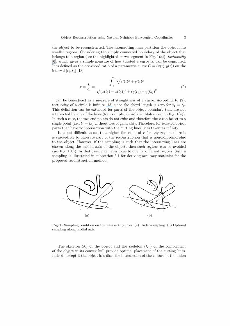
the object to be reconstructed. The intersecting lines partition the object intosmaller regions. Considering the simply connected boundary of the object thatbelongs to a region (see the highlighted curve segment in Fig. 1(a)), tortuousity[6], which gives a simple measure of how twisted a curve is, can be computed.It is defined as the arc-chord ratio of a parametric curve C = (x(t), y(t)) on theinterval [t0, t1] [13]

τ = L

C=

∫ t1

t0

√x′(t)2 + y′(t)2√

(x(t1)− x(t0))2 + (y(t1)− y(t0))2. (2)

τ can be considered as a measure of straightness of a curve. According to (2),tortuosity of a circle is infinite [13] since the chord length is zero for t1 = t0.This definition can be extended for parts of the object boundary that are notintersected by any of the lines (for example, an isolated blob shown in Fig. 1(a)).In such a case, the two end points do not exist and therefore these can be set to asingle point (i.e., t1 = t0) without loss of generality. Therefore, for isolated objectparts that have no intersection with the cutting lines, τ is taken as infinity.

It is not difficult to see that higher the value of τ for any region, more itis susceptible to generate part of the reconstruction that is non-homeomorphicto the object. However, if the sampling is such that the intersecting lines arechosen along the medial axis of the object, then such regions can be avoided(see Fig. 1(b)). In that case, τ remains close to one for different regions. Such asampling is illustrated in subsection 5.1 for deriving accuracy statistics for theproposed reconstruction method.

(a) (b)

Fig. 1. Sampling condition on the intersecting lines. (a) Under-sampling. (b) Optimalsampling along medial axis.

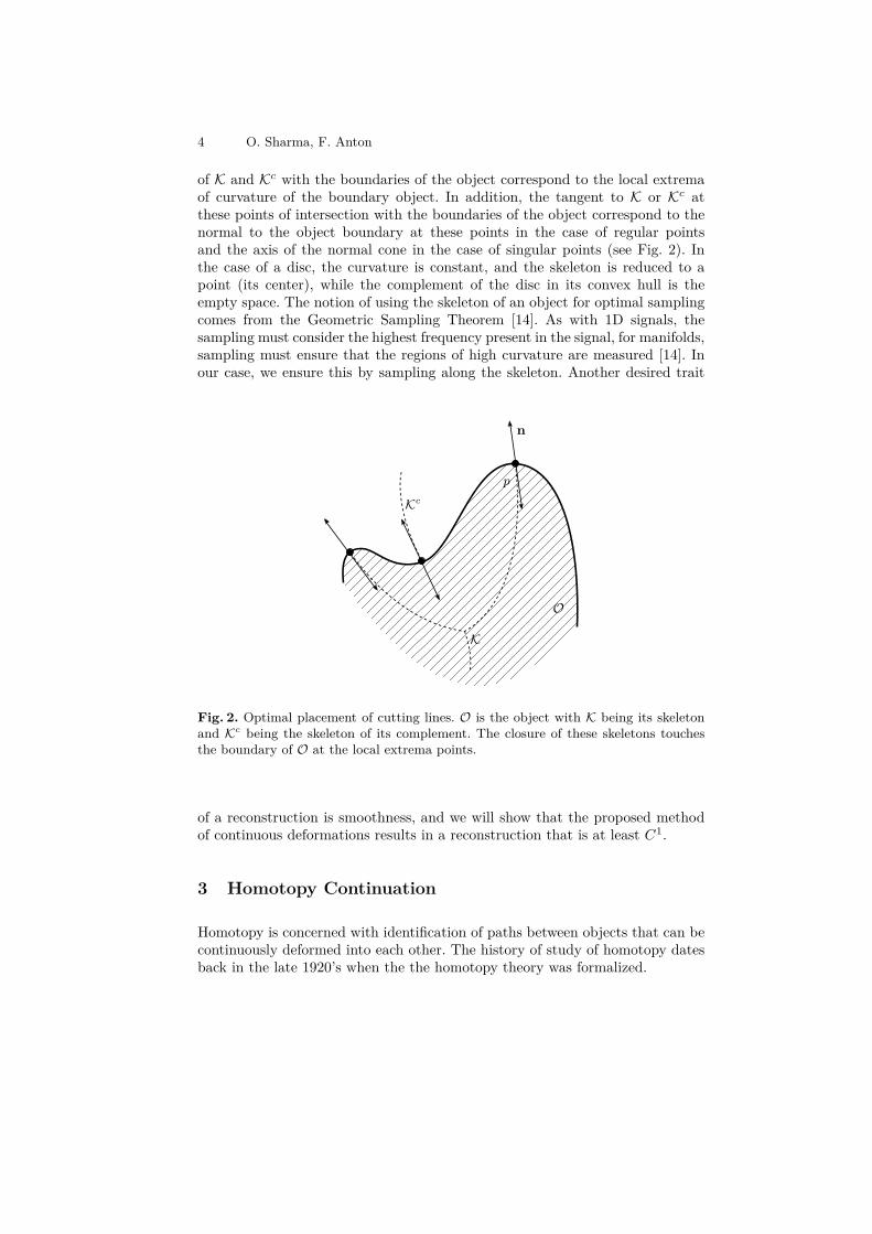
The skeleton (K) of the object and the skeleton (Kc) of the complementof the object in its convex hull provide optimal placement of the cutting lines.Indeed, except if the object is a disc, the intersection of the closure of the union

4 O. Sharma, F. Anton

of K and Kc with the boundaries of the object correspond to the local extremaof curvature of the boundary object. In addition, the tangent to K or Kc atthese points of intersection with the boundaries of the object correspond to thenormal to the object boundary at these points in the case of regular pointsand the axis of the normal cone in the case of singular points (see Fig. 2). Inthe case of a disc, the curvature is constant, and the skeleton is reduced to apoint (its center), while the complement of the disc in its convex hull is theempty space. The notion of using the skeleton of an object for optimal samplingcomes from the Geometric Sampling Theorem [14]. As with 1D signals, thesampling must consider the highest frequency present in the signal, for manifolds,sampling must ensure that the regions of high curvature are measured [14]. Inour case, we ensure this by sampling along the skeleton. Another desired trait

Kc

K

O

p

n

Fig. 2. Optimal placement of cutting lines. O is the object with K being its skeletonand Kc being the skeleton of its complement. The closure of these skeletons touchesthe boundary of O at the local extrema points.

of a reconstruction is smoothness, and we will show that the proposed methodof continuous deformations results in a reconstruction that is at least C1.

3 Homotopy Continuation

Homotopy is concerned with identification of paths between objects that can becontinuously deformed into each other. The history of study of homotopy datesback in the late 1920’s when the the homotopy theory was formalized.

Object Reconstruction using Natural Neighbor Barycentric Coordinates 5

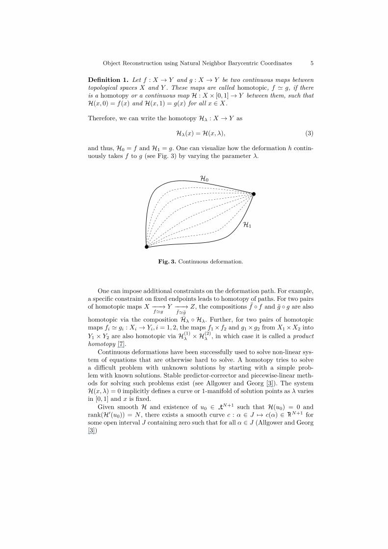
Definition 1. Let f : X → Y and g : X → Y be two continuous maps betweentopological spaces X and Y . These maps are called homotopic, f ' g, if thereis a homotopy or a continuous map H : X × [0, 1]→ Y between them, such thatH(x, 0) = f(x) and H(x, 1) = g(x) for all x ∈ X.

Therefore, we can write the homotopy Hλ : X → Y as

Hλ(x) = H(x, λ), (3)

and thus, H0 = f and H1 = g. One can visualize how the deformation h contin-uously takes f to g (see Fig. 3) by varying the parameter λ.

Fig. 3. Continuous deformation.

One can impose additional constraints on the deformation path. For example,a specific constraint on fixed endpoints leads to homotopy of paths. For two pairsof homotopic maps X −−−→

f'gY −−−→

f'gZ, the compositions f ◦ f and g ◦ g are also

homotopic via the composition Hλ ◦ Hλ. Further, for two pairs of homotopicmaps fi ' gi : Xi → Yi, i = 1, 2, the maps f1×f2 and g1× g2 from X1×X2 intoY1 × Y2 are also homotopic via H(1)

λ ×H(2)λ , in which case it is called a product

homotopy [7].Continuous deformations have been successfully used to solve non-linear sys-

tem of equations that are otherwise hard to solve. A homotopy tries to solvea difficult problem with unknown solutions by starting with a simple prob-lem with known solutions. Stable predictor-corrector and piecewise-linear meth-ods for solving such problems exist (see Allgower and Georg [3]). The systemH(x, λ) = 0 implicitly defines a curve or 1-manifold of solution points as λ variesin [0, 1] and x is fixed.

Given smooth H and existence of u0 ∈ RN+1 such that H(u0) = 0 and

rank(H′(u0)) = N , there exists a smooth curve c : α ∈ J 7→ c(α) ∈ RN+1 forsome open interval J containing zero such that for all α ∈ J (Allgower and Georg[3])

6 O. Sharma, F. Anton

1. c(0) = u0,2. H(c(α)) = 0,3. rank(H′(c(α))) = N ,4. c′(α) 6= 0.

In this work, we use homotopy or continuous deformations for object recon-struction. This is discussed in the next section.

4 Reconstruction Algorithm

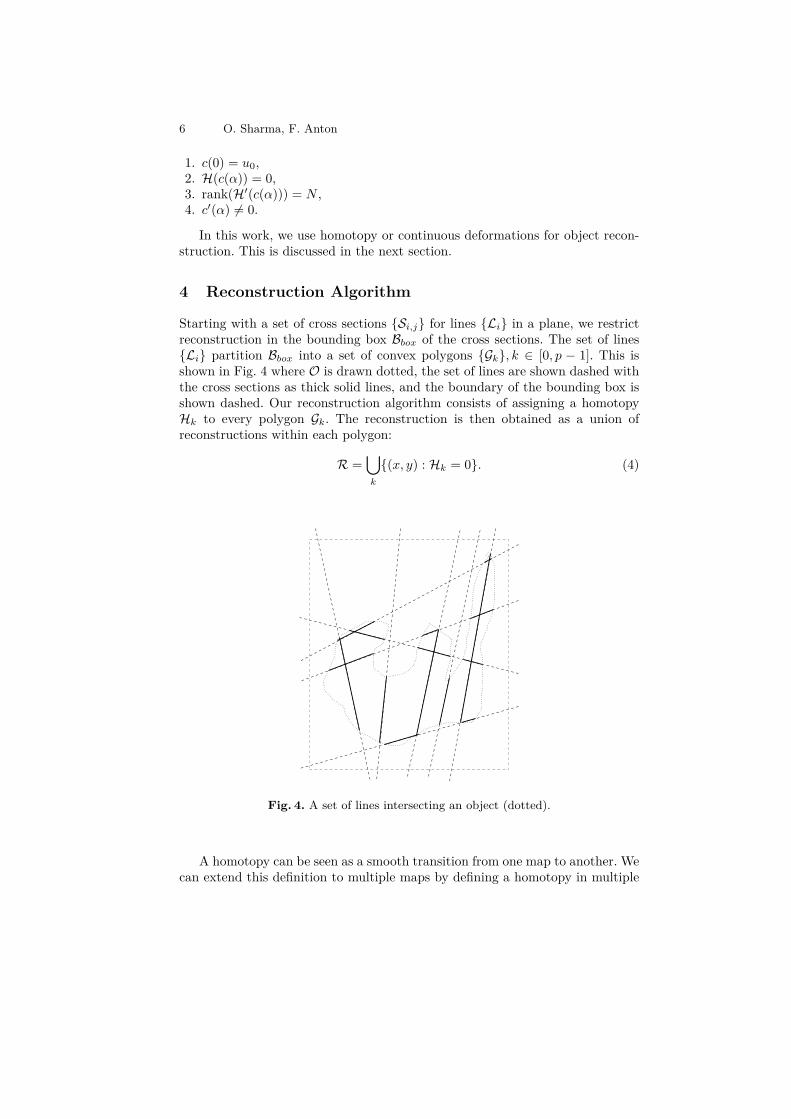
Starting with a set of cross sections {Si,j} for lines {Li} in a plane, we restrictreconstruction in the bounding box Bbox of the cross sections. The set of lines{Li} partition Bbox into a set of convex polygons {Gk}, k ∈ [0, p − 1]. This isshown in Fig. 4 where O is drawn dotted, the set of lines are shown dashed withthe cross sections as thick solid lines, and the boundary of the bounding box isshown dashed. Our reconstruction algorithm consists of assigning a homotopyHk to every polygon Gk. The reconstruction is then obtained as a union ofreconstructions within each polygon:

R =⋃k

{(x, y) : Hk = 0}. (4)

Fig. 4. A set of lines intersecting an object (dotted).

A homotopy can be seen as a smooth transition from one map to another. Wecan extend this definition to multiple maps by defining a homotopy in multiple

Object Reconstruction using Natural Neighbor Barycentric Coordinates 7

variables

H(λ0, λ1, · · · , λs−1) =s−1∑t=0

ftλt, (5)

withs−1∑t=0

λt = 1. (6)

The homotopy parameters must sum up to unity in order to define the defor-mation H inside the convex hull of the domain. In our case, the domain is apolygon formed by straight line segments.

4.1 Edge Maps

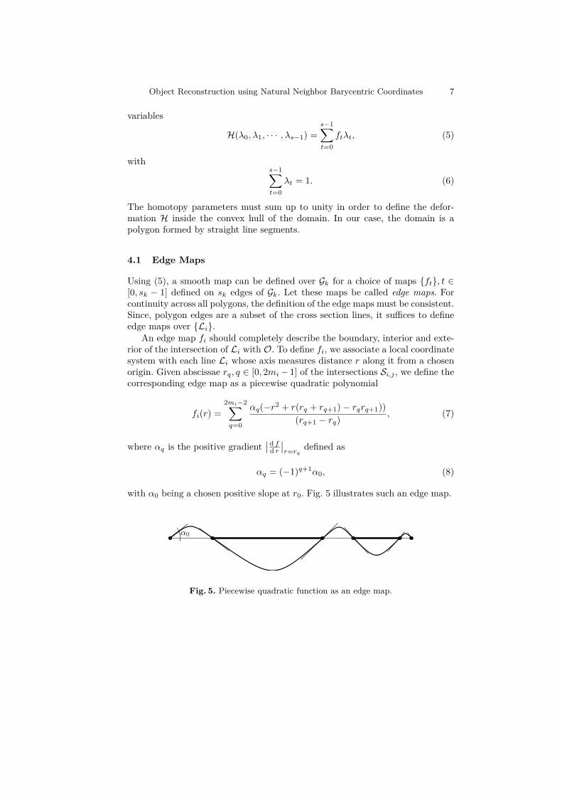
Using (5), a smooth map can be defined over Gk for a choice of maps {ft}, t ∈[0, sk − 1] defined on sk edges of Gk. Let these maps be called edge maps. Forcontinuity across all polygons, the definition of the edge maps must be consistent.Since, polygon edges are a subset of the cross section lines, it suffices to defineedge maps over {Li}.

An edge map fi should completely describe the boundary, interior and exte-rior of the intersection of Li with O. To define fi, we associate a local coordinatesystem with each line Li whose axis measures distance r along it from a chosenorigin. Given abscissae rq, q ∈ [0, 2mi− 1] of the intersections Si,j , we define thecorresponding edge map as a piecewise quadratic polynomial

fi(r) =2mi−2∑q=0

αq(−r2 + r(rq + rq+1)− rqrq+1))(rq+1 − rq)

, (7)

where αq is the positive gradient∣∣d f

d r∣∣r=rq

defined as

αq = (−1)q+1α0, (8)

with α0 being a chosen positive slope at r0. Fig. 5 illustrates such an edge map.

α0

Fig. 5. Piecewise quadratic function as an edge map.

8 O. Sharma, F. Anton

4.2 Barycentric Coordinates

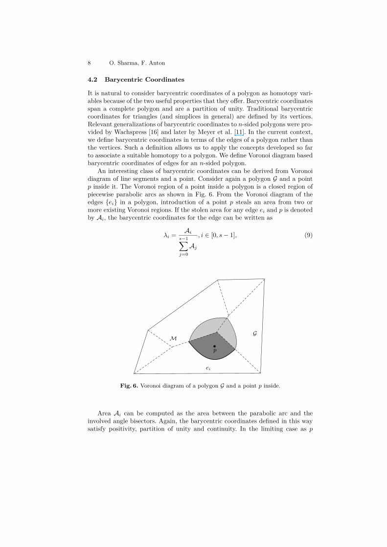
It is natural to consider barycentric coordinates of a polygon as homotopy vari-ables because of the two useful properties that they offer. Barycentric coordinatesspan a complete polygon and are a partition of unity. Traditional barycentriccoordinates for triangles (and simplices in general) are defined by its vertices.Relevant generalizations of barycentric coordinates to n-sided polygons were pro-vided by Wachspress [16] and later by Meyer et al. [11]. In the current context,we define barycentric coordinates in terms of the edges of a polygon rather thanthe vertices. Such a definition allows us to apply the concepts developed so farto associate a suitable homotopy to a polygon. We define Voronoi diagram basedbarycentric coordinates of edges for an n-sided polygon.

An interesting class of barycentric coordinates can be derived from Voronoidiagram of line segments and a point. Consider again a polygon G and a pointp inside it. The Voronoi region of a point inside a polygon is a closed region ofpiecewise parabolic arcs as shown in Fig. 6. From the Voronoi diagram of theedges {ei} in a polygon, introduction of a point p steals an area from two ormore existing Voronoi regions. If the stolen area for any edge ei and p is denotedby Ai, the barycentric coordinates for the edge can be written as

λi = Ais−1∑j=0Aj

, i ∈ [0, s− 1], (9)

p

GM

ei

Fig. 6. Voronoi diagram of a polygon G and a point p inside.

Area Ai can be computed as the area between the parabolic arc and theinvolved angle bisectors. Again, the barycentric coordinates defined in this waysatisfy positivity, partition of unity and continuity. In the limiting case as p

Object Reconstruction using Natural Neighbor Barycentric Coordinates 9

approaches one of the sides ek, the stolen area Ak becomes very small, but si-multaneously areas Ai,i 6=k become smaller (and eventually zero) by a rate higherthan that of the former. Thus as p approaches ek, λk → 1, and λi,i 6=k → 0.

4.3 Homotopy

Equipped with the above defined edge maps and barycentric coordinates for anypolygon Gk, we define a homotopy Hk in sk variables as

Hk(p) =sk−1∑i=0

fi (di(p))λi(p), (10)

where di(p) is the distance along line Lk from a chosen origin Ok on it until thefoot of the perpendicular from point p . We can write

di(p) = ||Ok − pi||+ (p− pi)T(pi+1 − pi)

li, (11)

where pi+1 and pi are two end points of an edge ei of Gk lying on Lk, and||x|| denotes the length of a vector x. Homotopy (10) continuously deforms edgemaps fi within the polygon and thus generates a smooth field. It can be seen asa linear combination of edge maps fi with barycentric coordinates λi. We canfurther extend this so called linear homotopy to a non-linear homotopy as

Hk(p, η) =sk−1∑i=0

fi (di(p))λi(p)η, (12)

with η as a parameter.Across polygons, the homotopy (10) is continuous and is at least C1 smooth

(see Appendix A for the proof). However, at all the intersection points Q ={Qi,j : Qi,j ∈ Li

⋂∂O} of the lines {Li} and the boundary ∂O of the object O,

the generated curve H−1(0) is orthogonal to any line in {Li} (see Appendix A).Therefore, the resulting reconstruction is somewhat unnatural. Given normals atthe intersection points Q (which is the case with many range scanning physicaldevices), we propose a tangent alignment scheme for the resulting curve bylocally warping the domain of the homotopies.

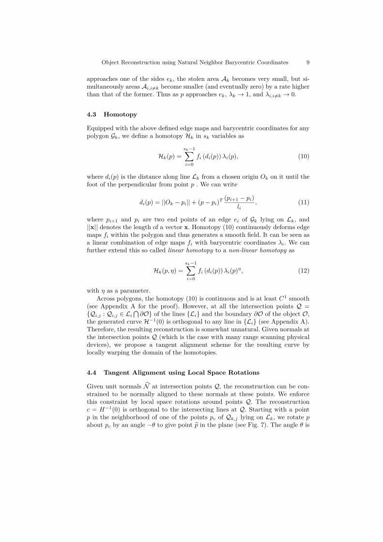
4.4 Tangent Alignment using Local Space Rotations

Given unit normals N at intersection points Q, the reconstruction can be con-strained to be normally aligned to these normals at these points. We enforcethis constraint by local space rotations around points Q. The reconstructionc = H−1(0) is orthogonal to the intersecting lines at Q. Starting with a pointp in the neighborhood of one of the points pc of Qk,j lying on Lk, we rotate pabout pc by an angle −θ to give point p in the plane (see Fig. 7). The angle θ is

10 O. Sharma, F. Anton

Fig. 7. Rotation of a point for tangent alignment.

chosen to be the signed angle between N and ∇Lk at the point pc. The resultinghomotopy H for a polygon G can be written as

H =sk−1∑i=0

fi

(di

)λi, (13)

where,

di = di(p) = ||Ok − pi||+ (p− pi)T(pi+1 − pi)

li, and

λi = λi(p) = Ais−1∑j=0Aj

, i ∈ [0, s− 1].

The rotated point p can be written as

p =pc + R(−θ)(p− pc), (14)

where R is the rotation matrix

R(θ) =[

cos θ − sin θsin θ cos θ

]. (15)

The modified gradient of the homotopy field in the neighborhood of pc can benow computed using the chain rule as:

∇H =s−1∑i=0

(f ′i(di)∇diλi + fi(di)∇λi

). (16)

In the limit as point p → pc (or the orthogonal distance to Lk, µk → 0 ),using a similar derivation as given in Appendix A, we can write

limµk→0

∇H = f ′k(di)∇dk (17)

Object Reconstruction using Natural Neighbor Barycentric Coordinates 11

Computing the gradient of dk,

∇dk = ∇(

(p− pk)T (pk+1 − pk)lk

)= ∇

((pc + R(−θ)(p− pc)− pk)T (pk+1 − pk)

lk

)= R(−θ)T (pk+1 − pk)

lk= R(θ)∇dk (18)

Therefore,

limµk→0

∇H = f ′k(di)R(θ)∇dk (19)

We know that the gradient

limµk→0

∇H = f ′k(di)∇dk. (20)

From (20) and (19) it can be seen that in the limit µk → 0

∇H||∇H||

= R(θ)(∇H||∇H||

). (21)

Therefore, we can achieve the desired rotation of the reconstruction curve byrotating the local coordinates around the points Q in the opposite direction.

4.5 Smooth Rotations of the Reconstruction Curve

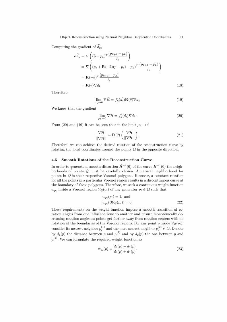
In order to generate a smooth distortion H−1(0) of the curve H−1(0) the neigh-borhoods of points Q must be carefully chosen. A natural neighborhood forpoints in Q is their respective Voronoi polygons. However, a constant rotationfor all the points in a particular Voronoi region results in a discontinuous curve atthe boundary of these polygons. Therefore, we seek a continuous weight functionwpi inside a Voronoi region VQ(pi) of any generator pi ∈ Q such that

wpi(pi) = 1, and

wpi(∂VQ(pi)) = 0. (22)

These requirements on the weight function impose a smooth transition of ro-tation angles from one influence zone to another and ensure monotonically de-creasing rotation angles as points get farther away from rotation centers with norotation at the boundaries of the Voronoi regions. For any point p inside VQ(pi),consider its nearest neighbor p(1)

i and the next nearest neighbor p(2)i ∈ Q. Denote

by d1(p) the distance between p and p(1)i and by d2(p) the one between p and

p(2)i . We can formulate the required weight function as

wpi(p) = d2(p)− d1(p)

d2(p) + d1(p) . (23)

12 O. Sharma, F. Anton

The first nearest neighbor p(1)i is the generator point pi of VQ(pi). The second

nearest neighbor p(2)i can be found by computing the second order voronoi di-

agram of Q. The weight function resulting from (23) is shown in Fig. 8. Weoutline the complete algorithm in Algorithm 1.

0.1

0.2

0.3

0.4

0.5

0.6

0.7

0.8

0.9

Fig. 8. Weights based on higher order Voronoi diagram.

5 Results

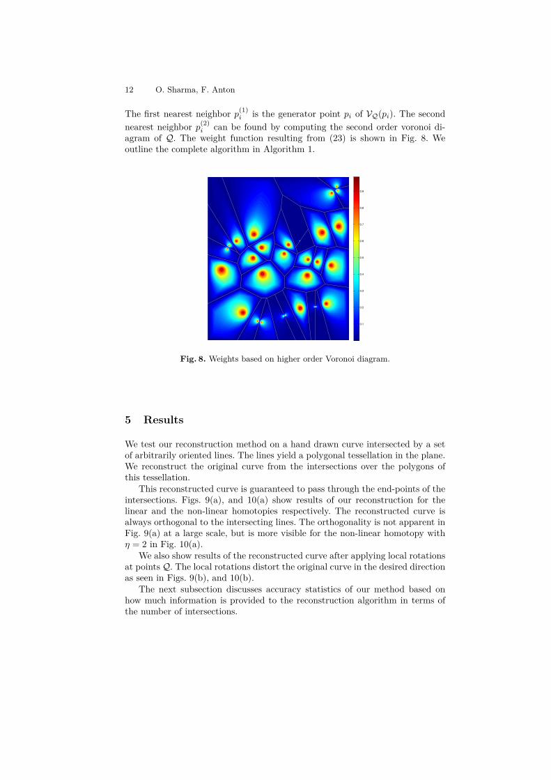
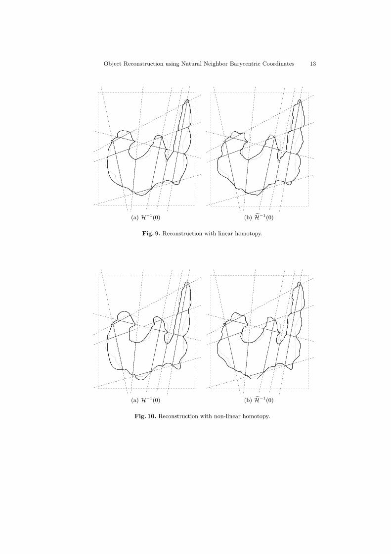
We test our reconstruction method on a hand drawn curve intersected by a setof arbitrarily oriented lines. The lines yield a polygonal tessellation in the plane.We reconstruct the original curve from the intersections over the polygons ofthis tessellation.

This reconstructed curve is guaranteed to pass through the end-points of theintersections. Figs. 9(a), and 10(a) show results of our reconstruction for thelinear and the non-linear homotopies respectively. The reconstructed curve isalways orthogonal to the intersecting lines. The orthogonality is not apparent inFig. 9(a) at a large scale, but is more visible for the non-linear homotopy withη = 2 in Fig. 10(a).

We also show results of the reconstructed curve after applying local rotationsat points Q. The local rotations distort the original curve in the desired directionas seen in Figs. 9(b), and 10(b).

The next subsection discusses accuracy statistics of our method based onhow much information is provided to the reconstruction algorithm in terms ofthe number of intersections.

Object Reconstruction using Natural Neighbor Barycentric Coordinates 13

(a) H−1(0) (b) H−1(0)

Fig. 9. Reconstruction with linear homotopy.

(a) H−1(0) (b) H−1(0)

Fig. 10. Reconstruction with non-linear homotopy.

14 O. Sharma, F. Anton

Input: {Si,j} on {Li}, N at QOutput: RDefine an edge map fi on each Li using {Si,j}Partition Bbox into polygonal tiles {Gk} with {Li}Compute first order Voronoi diagram V1

Q of QCompute second order Voronoi diagram V2

Q of QCompute w from V1

Q and V2Q

for k ∈ [0, p− 1] doCompute Voronoi diagram Vk of Gk

for x ∈ Gk doLet xc ∈ Q be the generator of Voronoi polygon of xx← xc + R(−θ)(x− xc)Compute {λi(x)} for all edges of Gk using Vk

Compute di(x) for all edges of Gk

Compute Hk

endendH ←

⋃Hk

R← ker HAlgorithm 1: The reconstruction algorithm.

5.1 Reconstruction Accuracy

A good reconstruction depends on the choice of cutting lines placed carefullyto cover salient geometric features of the object to be reconstructed. In orderto test the reconstruction algorithm for accuracy, we sample intersecting linesfrom the skeleton of the test object. We choose to sample the skeleton of theobject since it captures the salient details of the object. To show the dependenceof reconstruction accuracy on the number of intersecting lines, a hierarchy ofskeletons is used.

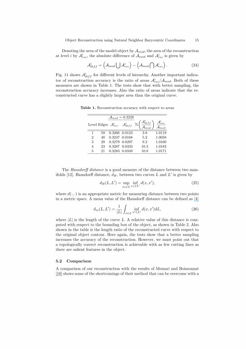
A skeleton hierarchy is computed from a straight line skeleton [2]. The hierar-chy provides an incremental simplification of the skeleton based on discrete curveevolution of the skeleton branches [8, 5]. Curve simplification by discrete curveevolution uses local angles at every vertex of the curve to assign a relevance toeach vertex. Based on the computed relevance values, the curve is evolved (sim-plified) by deletion of vertices. Fig. 11 shows such a skeleton hierarchy with fivelevels. The base skeleton is computed using the straight line skeleton module ofthe CGAL library [1] .

Sampled segments from the skeleton at every level are used as cutting linesfor reconstruction. Thus, for every level of hierarchy of skeletons, we compute areconstruction of the object. We next compute various error metrics for differentreconstructions thus obtained. To get a comprehensive idea of the reconstructionaccuracy, metrics based on area, mean distance error, and curve lengths areconsidered here.

Object Reconstruction using Natural Neighbor Barycentric Coordinates 15

Denoting the area of the model object by Amod, the area of the reconstructionat level i by Airec, the absolute difference of Amod and Airec is given by

Aidiff =(Amod

⋃Airec

)−(Amod

⋂Airec

). (24)

Fig. 11 shows Aidiff for different levels of hierarchy. Another important indica-tor of reconstruction accuracy is the ratio of areas Airec/Amod. Both of thesemeasures are shown in Table 1. The tests show that with better sampling, thereconstruction accuracy increases. Also the ratio of areas indicate that the re-constructed curve has a slightly larger area than the original curve.

Table 1. Reconstruction accuracy with respect to areas

Amod = 0.3228

Level Edges Airec Ai

diff %(Ai

diff

Amod

)Ai

rec

Amod

1 59 0.3266 0.0123 3.8 1.01192 40 0.3247 0.0168 5.2 1.00583 29 0.3279 0.0297 9.2 1.01604 23 0.3287 0.0333 10.3 1.01825 21 0.3283 0.0349 10.8 1.0171

The Hausdorff distance is a good measure of the distance between two man-ifolds [12]. Hausdorff distance, dH , between two curves L and L′ is given by

dH(L,L′) = supx0∈L

infx1∈L′

d(x, x′), (25)

where d(·, ·) is an appropriate metric for measuring distance between two pointsin a metric space. A mean value of the Hausdorff distance can be defined as [4]

dm(L,L′) = 1|L|

∫x∈L

infx′∈L′

d(x, x′)dL, (26)

where |L| is the length of the curve L. A relative value of this distance is com-puted with respect to the bounding box of the object, as shown in Table 2. Alsoshown in the table is the length ratio of the reconstructed curve with respect tothe original object contour. Here again, the tests show that a better samplingincreases the accuracy of the reconstruction. However, we must point out thata topologically correct reconstruction is achievable with as few cutting lines asthere are salient features in the object.

5.2 Comparison

A comparison of our reconstruction with the results of Memari and Boissonnat[10] shows some of the shortcomings of their method that can be overcome with a

16 O. Sharma, F. Anton

(a) Level 1 with 59 edges (b) Level 2 with 40 edges

(c) Level 3 with 29 edges (d) Level 4 with 23 edges

(e) Level 5 with 21 edges

Fig. 11. Skeleton hierarchy and reconstruction accuracy

Object Reconstruction using Natural Neighbor Barycentric Coordinates 17

Table 2. Reconstruction accuracy with respect to lengths

Level Edges %(

dH

Ldiag

)Li

rec

Lmod

1 59 0.75 1.08422 40 0.82 1.09193 29 1.02 1.12274 23 1.08 1.11915 21 1.11 1.1186

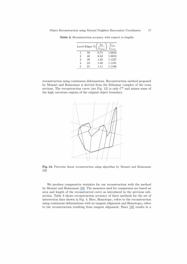
reconstruction using continuous deformations. Reconstruction method proposedby Memari and Boissonnat is derived from the Delaunay complex of the crosssections. The reconstruction curve (see Fig. 12) is only C0 and misses some ofthe high curvature regions of the original object boundary.

Fig. 12. Piecewise linear reconstruction using algorithm by Memari and Boissonnat[10]

We produce comparative statistics for our reconstruction with the methodby Memari and Boissonnat [10]. The measures used for comparison are based onarea and length of the reconstructed curve as introduced in the previous sub-section. Table 3 shows reconstruction accuracy of three methods for the set ofintersection lines shown in Fig. 4. Here, Homotopy1 refers to the reconstructionusing continuous deformations with no tangent alignment and Homotopy2 refersto the reconstruction resulting from tangent alignment. Since [10] results in a

18 O. Sharma, F. Anton

piecewise linear reconstruction, the area (possibly) and length of the curve areunderestimated. The ratio of absolute difference of area with the area of themodel is low for Memari’s reconstruction that matches up with Homotopy2 re-construction, but the relative Hausdorff measure goes bad and turns out to bemore than double of that obtained with either of the Homotopy based recon-structions. Further, the relative ratio of the lengths of the reconstruction andthe original object shows that homotopy based reconstructions perform betterwith estimating the length of the object.

Table 3. Comparison of Reconstructions

Method %(Adiff

Amod

) Arec

Amod%(

dH

Ldiag

)Lrec

Lmod

Memari [10] 14.6025 0.9652 3.9323 0.9149Homotopy1 17.5470 1.0407 1.4831 1.0256Homotopy2 14.6690 1.0425 1.3243 1.0303

6 Conclusion

In this work, we have presented a novel method of curve reconstruction fromarbitrary cross sections in a planar setting. The presented algorithm uses con-tinuous deformations to reconstruct the object smoothly. We also introducedgeneralized barycentric coordinates for polygons defined on its edges using theline and point Voronoi diagram. The presented method is general in nature andcan be applied to higher dimensions. We avaluate accuracy of our algorithmbased on sampling of the original object.

An interesting generalization of the problem of reconstruction from arbitrarycross sections is 3D reconstruction from arbitrary cutting planes. These cuttingplanes partition the domain of computation into polyhedra, and also embed theintersection with the object. Similar to the approach suggested in this paper,a function f : R2 7→ R can be embedded in a cutting plane such that ker(f)represents the boundary of this intersection. An example of one such functionis the signed distance function. Higher degree polynomial functions can be de-signed based on this distance function. A multi-variate homotopy can then beconstructed from the functions defined previously on the faces of a polyhedron. Apossible parameterization of such a homotopy is with respect to the orthogonaldistance of any point inside the polyhedron to the polyhedron faces (see Fig-ure 13). Parameterization in terms of the Voronoi volume (a volume consistingof a paraboloid face and planar faces) stolen by a point inside the polyhedron isanother choice. A union of the zero level set of the derived homotopies providesa reconstruction surface.

Object Reconstruction using Natural Neighbor Barycentric Coordinates 19

Fig. 13. Reconstruction from arbitrary cutting planes in R3. The polyhedron shows

one of the partitions of the domain resulting from cutting planes (one such shown here).The shaded region depicts the cross section of the 3D object with the cutting plane.

References

1. Cgal, Computational Geometry Algorithms Library, http://www.cgal.org2. Aichholzer, O., Aurenhammer, F., Alberts, D., Gartner, B.: A novel type of skeleton

for polygons. Journal of Universal Computer Science 1(12), 752–761 (1995)3. Allgower, E.L., Georg, K.: Numerical continuation methods: an introduction.

Springer-Verlag New York, Inc. New York, NY, USA (1990)4. Aspert, N., Santa-Cruz, D., Ebrahimi, T.: Mesh: Measuring errors between surfaces

using the hausdorff distance. In: Proceedings of the IEEE International Conferenceon Multimedia and Expo. vol. 1, pp. 705–708 (2002)

5. Bai, X., Latecki, L., Liu, W.: Skeleton pruning by contour partitioning with discretecurve evolution. IEEE transactions on pattern analysis and machine intelligence29(3), 449–462 (2007)

6. Dougherty, G., Varro, J.: A quantitative index for the measurement of the tortu-osity of blood vessels. Medical Engineering & Physics 22(8), 567–574 (2000)

7. Janich, K.: Topology, Undergraduate texts in mathematics (1984)8. Latecki, L.J., Lakamper, R.: Polygon evolution by vertex deletion. In: Scale-Space

Theories in Computer Vision. Proc. of Int. Conf. on Scale-SpaceÕ99, volume LNCS1682. pp. 398–409. Springer (1999)

9. Liu, L., Bajaj, C., Deasy, J.O., Low, D.A., Ju, T.: Surface reconstruction fromnon-parallel curve networks. In: Computer Graphics Forum. vol. 27, p. 155 (2008)

10. Memari, P., Boissonnat, J.D.: Provably Good 2D Shape Reconstruction from Un-organized Cross-Sections. In: Computer Graphics Forum. vol. 27, pp. 1403–1410(2008)

11. Meyer, M., Lee, H., Barr, A., Desbrun, M.: Generalized barycentric coordinates onirregular polygons. Journal of graphics, gpu, and game tools 7(1), 13–22 (2002)

12. Munkres, J.: Topology (2nd Edition). Prentice Hall (1999)13. Patasius, M., Marozas, V., Lukosevicius, A., Jegelevicius, D.: Model based inves-

tigation of retinal vessel tortuosity as a function of blood pressure: preliminaryresults. In: Engineering in Medicine and Biology Society, 2007. 29th Annual Inter-national Conference of the IEEE. pp. 6459 –6462 (2007)

14. Saucan, E., Appleboim, E., Zeevi, Y.: Geometric approach to sampling and com-munication. Arxiv preprint arXiv:1002.2959 (2010)

15. Sidlesky, A., Barequet, G., Gotsman, C.: Polygon Reconstruction from Line Cross-Sections. In: Canadian Conference on Computational Geometry (2006)

20 O. Sharma, F. Anton

16. Wachspress, E.L.: A rational finite element basis. Academic Press (1975)

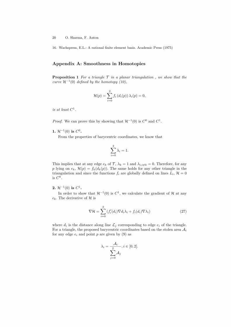
Appendix A: Smoothness in Homotopies

Proposition 1 For a triangle T in a planar triangulation , we show that thecurve H−1(0) defined by the homotopy (10),

H(p) =2∑i=0

fi (di(p))λi(p) = 0,

is at least C1.

Proof. We can prove this by showing that H−1(0) is C0 and C1.

1. H−1(0) is C0.From the properties of barycentric coordinates, we know that

2∑i=0

λi = 1.

This implies that at any edge ek of T , λk = 1 and λi,i 6=k = 0. Therefore, for anyp lying on ek, H(p) = fk(dk(p)). The same holds for any other triangle in thetriangulation and since the functions fi are globally defined on lines Li, H = 0is C0.

2. H−1(0) is C1.In order to show that H−1(0) is C1, we calculate the gradient of H at any

ek. The derivative of H is

∇H =2∑i=0

(f ′i(di)∇diλi + fi(di)∇λi) (27)

where di is the distance along line Lj corresponding to edge ei of the triangle.For a triangle, the proposed barycentric coordinates based on the stolen area Aifor any edge ei and point p are given by (9) as

λi = Ai2∑j=0Aj

, i ∈ [0, 2].

Object Reconstruction using Natural Neighbor Barycentric Coordinates 21

The gradient of λi can be calculated using the chain rule as

∇λi = ∇Ai2∑j=0Aj

− Ai 2∑j=0Aj

2

2∑j=0∇Aj

= ∇Ai2∑j=0Aj

− λi2∑j=0

∇Aj2∑j=0Aj

(28)

Using (27) and (28),

∇H =2∑i=0

f ′i(di)∇diλi + fi(di)

∇Ai2∑j=0Aj

− λi2∑j=0

∇Aj2∑j=0Aj

(29)

To compute the gradient of H at the intersection of line Lj and the object,we must take the derivative at a point p in the limit as p approaches line Lj . Inthis limit,

λk → 1λi,i6=k → 0 (30)

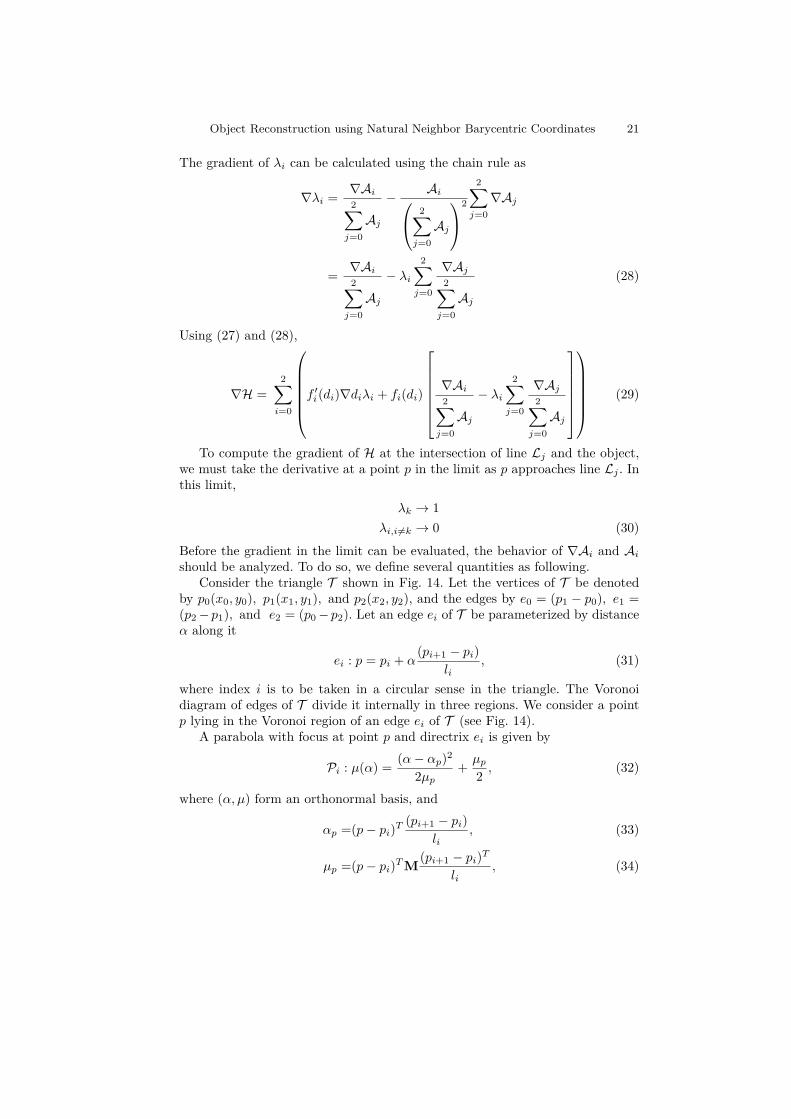
Before the gradient in the limit can be evaluated, the behavior of ∇Ai and Aishould be analyzed. To do so, we define several quantities as following.

Consider the triangle T shown in Fig. 14. Let the vertices of T be denotedby p0(x0, y0), p1(x1, y1), and p2(x2, y2), and the edges by e0 = (p1 − p0), e1 =(p2−p1), and e2 = (p0−p2). Let an edge ei of T be parameterized by distanceα along it

ei : p = pi + α(pi+1 − pi)

li, (31)

where index i is to be taken in a circular sense in the triangle. The Voronoidiagram of edges of T divide it internally in three regions. We consider a pointp lying in the Voronoi region of an edge ei of T (see Fig. 14).

A parabola with focus at point p and directrix ei is given by

Pi : µ(α) = (α− αp)2

2µp+ µp

2 , (32)

where (α, µ) form an orthonormal basis, and

αp =(p− pi)T(pi+1 − pi)

li, (33)

µp =(p− pi)TM (pi+1 − pi)T

li, (34)

22 O. Sharma, F. Anton

Fig. 14. Parameterization along triangle edge.

with

M =[

0 1−1 0

], (35)

and li is the length of ei.Let the parabola Pi intersects the boundary of the Voronoi region at points

bi(α0, µ0) and bi+1(α1, µ1) respectively. Denote by q(αq, µq) the incenter of T .The parabola can intersect the two angle bisectors of the triangle Bi : µ = k0α,and Bi+1 : µ = k1(li − α), ki = tan(θi/2), in three possible ways

I. α1 ≤ αq: both branches of the parabola intersect Bi, and µm = k0αm,m ={0, 1},

II. α0 ≥ αq: both branches of the parabola intersect Bi+1, and µm = k1(li −αm),m = {0, 1}, and

III. α0 < αq and α1 > αq: the branches of the parabola intersect Bi and Bi+1respectively, and µ0 = k0α0 and µ1 = k1(li − α1).

It is sufficient to treat one of these cases here. Considering case I, α0 and α1 arethe roots of

α2 − 2α(αp + k0µp) + (α2p + µ2

p) = 0. (36)

The areas to compute the barycentric coordinates can be written as

Ai = Apari +Atrii (37)

Object Reconstruction using Natural Neighbor Barycentric Coordinates 23

where, Apari is the area enclosed between the parabolic arc and line connectingbi and bi+1, and Atrii is the area of the triangle connecting points bi, bi+1, andq. Using (32)

Apari = µ0 + µ1

2 (α1 − α0)−∫ α1

α0

((α− αp)2

2µp+ µp

2

)dα, (38)

and

Atrii = µ0 + µq2 (αq − α0) + µ1 + µq

2 (α1 − αq)−µ0 + µ1

2 (α1 − α0). (39)

Therefore,

Ai = µ0 + µq2 (αq − α0) + µ1 + µq

2 (α1 − αq)−∫ α1

α0

((α− αp)2

2µp+ µp

2

)dα

(40)

Note that (40) holds for all the three cases above. Simplifying (40), we get

2Ai = (µ0 + µq)(αq − α0) + (µ1 + µq)(α1 − αq)−[

(α− αp)3

3µp− µpα

]α1

α0

= (µ0 + µq)(αq − α0) + (µ1 + µq)(α1 − αq)

− (α1 − αp)3 − (α0 − αp)3

3µp− µp(α1 − α0) (41)

Distance di in (10) can be written as

di(p) = ||Oj − pi||+ αp, (42)

where we know that pi lies on Lj and Oj is the chosen origin on Lj . We notethe following derivatives

2∇Ai = ∇α0(−µ0 − µp) +∇α1(µ1 + µp) +∇µ0(−α0 + αq) +∇µ1(α1 − αq)

+ (α1 − αp)3 − (α0 − αp)3

3µ2p

∇µp −(α1 − αp)2(∇α1 −∇αp)

µp

+ (α0 − αp)2(∇α0 −∇αp)µp

− (α1 − α0)∇µp − µp(∇α1 −∇α0) (43)

∇di = ∇αp = (pi+1 − pi)li

(44)

∇µp = M (pi+1 − pi)li

(45)

∇αm = ∇αp(αm − αp) +∇µp(µm − µp)(αm − αp − k0µp)

,m = {0, 1} (46)

∇µm = k0∇αm, m = {0, 1} (47)

24 O. Sharma, F. Anton

In the limit µp → 0 for some edge ek of T ,

αm → αp, m ∈ {0, 1}µm → k0αp m ∈ {0, 1} (48)

Consequently, Ai → 0, but Ai,i6=k becomes 0 much faster than Ak. Therefore,using (30) and (48), the gradient (29) in the limit is

limµp→0

∇H = f ′k(dk)∇dk + fk(dk)

∇Ak2∑j=0Aj

− ∇Ak2∑j=0Aj

= f ′k(dk)∇dk. (49)

Gradient of line ek is

∇ek = M (pi+1 − pi)li

. (50)

We note that⟨limµp→0

∇H,∇ek⟩

= f ′k(dk) (pi+1 − pi)T

liM (pi+1 − pi)

li

= 0.

A similar result can be shown for the gradient of the homotopy on the other sideof Lj . This implies that the reconstructed curve is orthogonal to the intersectinglines from either side.

Therefore, the curve reconstruction is at least C1. ut