Naval Research Laboratory

Washington, DC 20375-5000

NRL Memorandum Report 6456

Near-Neighbor Algorithms for Processing Bearing Data

J.M. PICONE, J.P. BoRIs, S.G. LAMBRAKOS, J. UHLMANN* AND M. ZUNIGA**

Center for Computational Physics DevelopmentsLaboratory for Computational Physics and Fluid Dynamics (LCPFD)

*Berkeley Research Associates, Springfield, VA 22150

0NJ **Science Applications International Corporation, McLean, VA 22102

oDTICE ALrEe CTrE publ May 10, 1989MAY 19 1989 LI

Approved f or public release: distribution unlimited.

SECURITY CLASSiFiCATiON OF THIS >AGEForm Acoroved

REPORT DOCUMENTATION PAGE OMB o 0704-0188

la. REPORT SECURITY CLASSIFICATION lb RESTRICTIVE MARKiNGSUNCLASSIFIED2a. SECURITY CLASSIFICATION AUTHORITY 3 DISTRIBUTION,'AVAILABILITY OF REPORT

2b. DECLASSIFICATION/DOWNGRADING SCHEDULE Approved for public release; distribution

unlimited.

4. PERFORMING ORGANIZATION REPORT NUMBER(S) S. MONITORING ORGANIZAT,0N PEPOR' '.t3E=S;

NRL Memorandum Report 6456

6a. NAME OF PERFORMING ORGANIZAT;ON 6o OFFCS SYMBOL 7a. NAME OF MONITORING "AN.Z.T -A

I (if applicable)Naval Research Laboratory Code 4440

6C. ADDRESS (City, State, and ZIP Coce) 7 7b. ADDRESS (City, Scare. ana ZIP Cooe)

Washington, DC 20375-5000

Ba. NAME OF FUNDING/SPONSORING B. OFFiCE SYMBOL 9 PROCUREMENT iNSTRUMENT IDENT;FICATOJ NUBER .- "-'ORGANIZATION (If applicable)

SD 10Sc. ADDRESS (City, State, and ZIP Code) 10 SOURCE OF FUNDING NUMBERS

PROGRAM PROJECT TAS K VORK JNT

Washington, DC 20301-7100 ELEMENT NO NO NO ACCESSION NO

11. TITLE (Include Security Classification)

Near-Neighbor Algorithms for Processing Bearing Data

12. PERSONAL AUTHOR(S)

Picone, J.M., Boris, J.P., Lambrakos, S.G.. Uhlmann,* J. and Zuniza,** M.13a. TYPE OF REPORT 13b TIME COVERED 14 DATE OF REPORT (Year, Month Day) 15 PGE COUN

Interim FROM 2/88 TO 2/89 1989 May 10 4916 SUPPLEMENTARY NOTATION

*Berkeley Research Associates, Springfield, VA 22150**Science Applications International Corporation, McLean, VA 2210217. COSATI CODES 18. SUBJECT TERMS (Continue on reverse of necessary and ,centiry Oy block number)

FIELD GROUP SUB-GROUP Near-neighbor algorithms Bearing dataPassive sensors Multisensor data fusion

19 ABSTRACT (Continue on reverse if necessary and identify by block number)

....- ---The authors discuss the use of near-neighbor algorithms for correlating sets of tracks

and sensor data on large numbers of rapidly moving objects. By investigating the scaling

of such algorithms with the numbers of elements in the data sets, one finds that near-

neighbor algorithms need not be universally more cost-effective than brute force methods.

While the data access time of near-neighbor techniques scales with the number of objects

N better than brute force, the cost of setting up the data structure could scale worse than

(Continues)

20 DISTRIBUTIONiAVAILABILITY OF ABSTRACT 21 ABSTRACT SECURITY CLASSI ,CAT,ONERUNCLASSIFED/UNLIMITED [:3 SAME AS RPT 0 DTIC USERS UNCLASSIFIED

22a NAME OF RESPONSIBLE INDIVIDUAL 22b TELEPHONE (Include Area Coce) _ C'iC- V iI.

J.M. Picone (202) 767-3055 Code !.L,4H.

DD Form 1473, JUN 86 Previous editions are obsolete -IS," .AS C- O " --> -c$I'' n!'n-L- '

''"

SECURITY CLASSIFICATION OF THIS PAGE . .

19. ABSTRACTS (Continued)

-tbrute force by a multiplicative factor of log N in an extreme case. For cases in which near-

neighbor algorithms are advantageous, the authors describe how such techniques could

be used to correlate three-dimensional tracks with bearing data recorded as two angles

(6, 0).from a single sensor. The paper then presents a high-speed algorithm for fusing

bearing data from three or more sensors with overlapping fields of view in order to obtain

the three-dimensional positions of the objects being observed. The algorithm permits the

use of near-neighbor techniques, reducing the scaling of the problem from N m to N In N,

where N is te number of objects in the common domain of observation, and m is the

number of sensors involved. Numerical tests indicate the relative efficiencies of typical

near-neighbor techniques in solving the multisensor angle-to-position fusion problem.

DO Form 1473, JUN 86 iReverse) zECuJRITN CLASSIF CA%ON CC "1 :GE

• , . l II I I i

CONTENTS

I. IN T R O D U C T IO N ................................................................................................... I

11. DATA CORRELATION IN MANY-BODY SCENARIOS ................................................. 3

11. WHY NEAR-NEIGHBOR ALGORITHMS .................................................................... !4

1.2 WHEN WILL NN ALGORITHMS WORK BEST FOR TRACKING AND CORRELATION ...... I

MII. SINGLE SENSOR BEARING DATA .................................................. . . ................ 15

M .I HOCKNEY 'S M ETHO D .......................................................................................... 15

M.2 THE MONOTONIC LAGRANGIAN GRID [3,51 .......................................................... 17

IV. THREE SENSORS WITH OVERLAPPING FIELDS OF VIEW ......................................... 22

IV. 1 TRANSFORMATION OF BEARING DATA TO NEW ANGLES ....................................... 24

IV.2 REPRESENTATIVE ALGORITHMS AND TESTS ......................................................... 28

IV.3 PERFORMANCE RESULTS ON A SUN-260 WORKSTATION ....................................... 31

V.4 CONCLUSIONS FROM TESTS ........................................................... . . ............... 35

IV.5 ESTIMATES OF PERFORMANCE ON OTHER HARDWARE ......................................... 35

V . SU M M A R Y ............................................................ .. ......................... 37

VI. ACKNOW LEDGEM ENTS ....................................................................................... 38

R E FE R E N C E S ...................................................................................................... 39

APPENDIX - Details of Multisensor Bearing-to-Position Conversion .................................. 41

i ,,; T,, i

1A -

111(

NEAR-NEIGHBOR ALGORITHMS FOR PROCESSING BEARING DATA

I. Introduction

One of the more pressing problems in Correlator-Tracker (CT) algorithms is the ef-

ficient use of sensor data consisting of only the bearings of objects relative to the sensor.

By assumption, no range information is available, or the range is much less accurately

known than the bearing. Infrared sensors will produce bearing data, for example. Here

we present recent progress in processing and using such data. The paper emphasizes use

of data structures designed for ready access of information on the near neighbors of each

object, such as a track or contact report, within an ensemble. Implicit in the discussion is

the perceived need for optimization on highly parallel or vector computers of the present

and future in order to handle tens or hundreds of thousands of objects as rapidly as possi-

ble. The goal is to perform the same calculation simultaneously on large subsets of these

objects.

Since the likelihood of association of a track with a sensor observation or "report" de-

creases with track-report separation, one usually assumes that rapid access of near neigh-

bors will drastically reduce the work required in updating tracks through the use of new

sensor data. The next section discusses the conditions under which the use of near-neighbor

(NN) algorithms is actually advantageous. This discussion also indicates conditions under

which the use of NN techniques might not be advisable. Section III then considers the

correlation of bearing data with tracks in three-dimensional space. Section IV shows how

to use bearing data derived from sensors with overlapping fields of view to determine the

three-dimensional positions of the objects within the common domain of observation. Here

the pivotal innovation is the reduction of the problem from enumerating the intersections

of bearing vectors recorded by different sensors to evaluating the equality of pairs of special

angles computed from the bearing data. This format facilitates the use of near-neighbor

searches and fast sorting algorithms and vastly reduces the computer time required.

The reader should note that the term "track" might be used here in a less precise sense

than the designers of correlator-tracker software might desire. Define the term "target

Manuscnpt approved March 14. 1989.

map" to be the statistical representation of a state vector at a given time for a possibie

object, as determined from sensor contact reports [1]. A track is then a time sequence of

target maps corresponding to the same object. The statistical nature of the target map

derives from errors implicit in the measurement and estimation process. To determine

near neighbors in the present paper, the authors use the mean locations (or expectation

values of the respective positions) of the contact reports and target maps. Further, the

term "track" stands for the mean location of the taxget map at a given time t.

2

IL Data Correlation in Many-Body Scenarios

In this discussion, a data set will contain "data elements," each of which corresponds to

one of a set of objects being observed. Thus each data element can be a contact report from

one of an array of sensors covering a region of physical space or a target map produced by a

correlator-tracker from such data. The statement that two data elements are *correlated"

means that each data element describes or pertains to the same physical object with a

likelihood that exceeds some threshold value. The statement that two disjoint sets of data

elements are "related" means that each of the sets contains at least one data element that

is correlated to a data element of the other.

The problem considered here is stated as follows: given M > 2 related, disjoint

sets of data (denoted S1, S2, ... ,SM), find the elements of the respective sets which are

correlated with each other. That is, find all sets {ai, bj, ... , Cm} where ai E Si, bj E

S2, ... , and cm E SM, so that ai, bj, ... , cm are all correlated. "Data correi.tion" or

simply "correlation" is the process of identifying correlated data elements. In practice, the

determination that two elements of different data sets are correlated can be approximate

(probability of correlation less than one), and estimating the degree of correlation requires

the calculation of a correlation score. As indicated above, one example is the act of finding

the track (constructed from previous data) which is correlated with a new sensor contact

report. Upon establishing this relationship, one can extend the track to later times, using

the new contact report to refine the track.

The relevant scenarios comprise tens to hundreds of thousands of rapidly moving ob-

jects. We further assume that the period under consideration is a few hours at most.

Because of the large numbers, high speeds and short time scales involved, time delays

of even a minute in data processing could be too large to react to the situation. One

thus immediately concludes that data correlation in this case requires highly parallel com-

puters with large amounts of memory, so the requisite data processing can be as nearly

instantaneous as possible. Only analysis and numerical simulations of realistic scenarios

3

containing such large numbers of objects can provide estimates of the computing needs in

this situation.

11.1 Why Near-Neighbor Algorithms?

Work has begun on the development of highly parallel correlation algorithms under the

assumption that scalar algorithms and hardware would not be adequate for the scenarios

mentioned above. The parallel environment would permit groups of correlation calculations

to be performed simultaneously. Ideally the individual data elements involved in the

parallel calculation correspond to the same observation time or nearly the same observatic-

time t0 . This is where near-neighbor algorithms offer the greatest advantage over brute

force methods.

A "brute force" method computes a correlation score for all possible sets

{ai, bj, ... , cm}. When the data sets S1, S 2 , ... ,SM, contain the same number of elements

N1 = N 2 - ... " NM = N, the brute force calculation scales as NM, where I is the

number of data sets to be correlated at one time. This paper considers problems for which

M = 2 or 3.

A "near-neighbor" algorithm is a method for storing and accessing data on N objects

so that the following conditions hold:

(1) Storage and access of data depends on object parameters: for example, position, ve-

locity, or attributes. In a dynamical system, time can either be explicit or implicit in the

near-neighbor data structure.

(2) The storage and access depend on indexing the data or pointers to the data (a "data

structure") so that the indices themselves contain information on parameter values; and

(3) On average, scaling of the access time with N is better than "brute force" methods by

a factor of approximately N/log N or better.

Near-neighbor algorithms eliminate an appreciable fraction of the combinations

ai,, bp ... , c,} from consideration before correlation scores are computed. Consider

4

the case M = 2. For each ai E S1, one accesses only the data elements in S2 which

satisfy definite criteria for being near neighbors of ai. The resulting subset of S2 is

NN21(i) =_ {b31 bi NN of a1 } C S2 and the correlation score is computed only for the

near neighbors NN2 1 (i). Depending on the particular NN algorithm, the cost of accessing

near neighbors for each ai E S1 scales as either N' (constant) or inN. So the cost for N

such calculations (all elements of S1) scales as N or NlnN, both of which are less than

brute force scaling. For N = 10, 000 objects and M = 2, the use of NN algorithms gives a

potential improvement of three to four orders of magnitude over the brute force approach.

For M = 3, the improvement can be seven to eight orders of magnitude.

To summarize the above discussion, a near-neighbor algorithm involves the construc-

tion and use of an intermediate data structure which permits the rapid identification of

likely candidates (usually a relatively small number) for correlation with a given data el-

ement before the actual correlation score calculation is done. If the same near-neighbor

data structure is used for all data accesses, the scaling with N, the number of elements in

a data set, is faster by several orders of magnitude than is a brute force algorithm, when

N is I-gZ.

Table 1 lists near neighbor algorithms that the authors have developed or tested. The

quantity N is the number of elements of set S1, all of which reside in the near-neighbor

data structure. Column 2 shows the scaling of the time required to set up the NN data

structure. The scaling of the cost for accessing near neighbors of a given element of S.

appears in the third column. For this operation, NN algorithms are superior to brute

force. On the other hand, column 2 indicates that if only a few accesses occur before

the data structure must be set up again or reconstructed, the total cost of using a near

neighbor algorithm could scale more poorly with N than brute force. The NN algorithm

is not necessarily optimal in every case. For use of a NN algorithm to be beneficial, the

cost of organizing the data according to a NN data structure and computing scores for the

resulting limited subsets of S, ® S2 must be less than the total cost (over the entire set

S2) of comparing all elements bj of S2 with all elements ai of S1.

5

0 z z z z

*

QPJ)

vi -

C12I,

Li- -

z z z .- .-

z 0o 0

C12 z z zLi

~,-

:Li~

0

Li

QLi

0

0 Li.4-4--o

0 Li Li0

6

1H.2. When Will NN Algorithms Work Best for Tracking and Correlation?

To see how NN algorithms can increase the speed of data correlation, one can analyze

the following equation for the cost in computer time of correlating all N2 elements of set

S2 with all N 1 elements of S1 :

c=C , + C,. -. 2.-,

In Eq.(2.2.1), C,. is the cost of finding the elements bj E S2 which are near neigh.bors

of the respective ai E SI; and C, is the time required to compute scores for all of the

NN pairings {aj, b,} E NN 2 1(i), for i = 1, 2, ... , N 1 . The scaling of each term with N1

and N 2 provides a basis for initial comparison of NN algorithms with brute force methods.

The constant coefficients multiplying the scaling functions will vary with the cornuter

hardware and the degree to which the software is optimum for that hardware.

In the context of correlation and tracking, define set S, as the set SR of contact

reports, corresponding in the most general case to different observation times {t, ; i =

1,2,... , Nr}, where N1 =- N,, the number of contact reports. The set S2 is then equal to

ST, the set of N-2 =- Nt tracks. Thus for each contact report ai E S, our objective is to

identify all tracks in S2 that are correlated with ai. The tracks in S2 all correspond *o

the same time ti, which is different from the observation times for the set {ai } in the most

general case. The computation of a correlation score requires that a track and a report

correspond to the same time [21, so that, in theory, the set of tracks must be extrapolated

to the time corresponding to each contact report ai E S1. The score can decrease on

average with track-report distance, but is not, in general, a function of the distance alone.

H.2.1. "Brute Force" Methods

A brute force method treats each contact report separately from the others an(i per-

forms calculations (not necessarily scores) for all possible pairings of tracks with contact

reports. Several brute force procedures are possible. Below we assume that e.trapolation

of each track to the time of each report is implicit in any brute force algorithm.

7

Procedure 1. For each contact report aj, compute the "distances" Dij to all tracks 5j.

For each track satisfying Dii < R, where R is a distance chosen to define near neighbors,

compute the correlation score. The scaling of the cost equation (2.2.1) with Nr and Vt is

In this equation, the coefficients .A are constant, and the superscript b signifes 'brute

force." The coefficient Ab depends on the average number of tracks found to be near

neighbors of each contact report and the cost of computing a score. Because the first step

of Procedure 1 culled out the tracks that were poor candidates for correlation, the second

term does not depend on Nt. The coefficients are important, since the actual correlation

calculation will be much more expensive than the calculation of distances in the first step.

Notice that the distances D i are straightforward to calculate only when physical positions

are used to defime "near neighbors". If other attributes are to be considered, the testing

might be on intervals of attribute values rather than on a normalized "distance" function.

A possible drawback of Procedure 1, as described above, is that the value of R is

somewhat arbitrary and in fact might have to be inefficiently large to ensure finding all

the correlations with acceptable scores. The reason is that the score is not a function of

R alone, additionally depending on the statistical distributions defining the track state

vector and the contact report. This means that some tracks with unacceptable correlation

values would be selected in the near-neighbor-access step of Procedure I. Alternatively

one could do a simple comparison to find all tracks within an initial radial interval (0, R0 )

of contact report a, and compute scores for this subset NN2 1 (i). Then choose a radius

R, > Ro. For the remainder of the tracks (the set S 2 - NN 21(i)), find the tracks in the

interval (Ro, R 1), compute their correlation scores, and eliminate those tracks from the

set of candidates for the next radial interval. This process continues to larger distances

RI until all correlation scores for the tracks in the interval (Rt, Ri+1 ) fall below a selected

threshhold. The size of the subset of S2 to be searched and the associated cost decrease

8

with successive radial intervals. In addition the algorithm should identify all correlations

with a score above the threshhold. Testing on realistic scenarios is necessary to determine

the efficiency of Procedure 1 relative to the procedures below.

Procedure 2. For each contact report ai, compute the full correlation score for all tracks.

Keep only those tracks with scores above some minimum acceptable value or threshold.

The scaling of the cost equation (2.2.1) with N, and Nt is

Cb = Ab N, Nt. (2.2.3)

Here no preliminary determination of near neighbors has occurred before the correlation

score calculation, so that Eq.(2.2.3) indicates greater cost than both parts of the previous

procedure, given that calculating the correlation score is the most expensive part of the

algorithm.

Procedure 3. For each contact report a,, compute and sort the distances Dij to all tracks,

and compute correlation scores in order of increasing distance until the score falls below a

minimum acceptable value. The cost of this is harder to quantify because the number of

scores calculated depends on a score threshhold instead of a distance threshhold. A useful

equation is

-- A N Nt + Ab'N, Nt InNt + Ab f Nt Nr. (2.2.4)

The coefficient Ab depends on the cost of computing a score. The quantity f is the average

fraction of the Nt tracks for which correlation scores must be calculated on a "per contact

report" basis. If f is sufficiently small, this procedure should cost less than Procedure 2.

In addition, if f - Nt-', where a > 0, then the scaling of the score calculation (third

term) is better than in Eq.(2.2.3). This method also eliminates the potential drawback of

Procedure I that the value chosen for R is somewhat arbitrary and in fact might have to

be chosen undesirably large to ensure finding all the correlations with acceptable values.

9

Notice that the first two terms have potentially more expensive scaling than the third

but that the coefficients A~'3 and Ab, In Nt could be much smaller than A' f . In addition,

the remote possibility exists that, even for large numbers of objects, the coefficients A

could be more important than the scaling with N,. and Nt.

Procedure 4. Here we mention a nonhierarchical cluster algorithm i, which is discussed

in a companion document [31 and analyzed fully there. This algorithm ideni.es arcxI uses

clusters containing tracks and reports which can only be associated with members of the

cluster in which they reside. Based on this information, the computation of correlation

scores has scaling ranging between N'12 and N 2 , depending almost entirely on the scenario.

We refer the reader to the above reference [3] for further information.

An important factor in the values of the coefficents for the above procedures is the

availability and type of computer hardware. The speed-up through parallelization and the

parallel implementation itself will likely vary with the particular calculation (each term

in the above equations). This could change the scaling with N in the cost equations

or change the relative importance of the individual terms. In addition, for particulz -

multiple-hypothesis-tracking (MHT) algorithms, some of the procedures above might no'

be possible or acceptable. Most importantly for the brute force algorithms, the processing

of each contact report will be the same whether the contact report time stamps {ti} are

different or not. This could result in an advantage over near-neighbor algorithms, which

are considerably more efficient when many of the contact reports have approximately the

same time stamps.

11.2.2 Near-Neighbor (NN) Algorithms

As indicated earlier, NN Algorithms are best suited for processing groups of contact

reports in a parallel or vector fashion. The constraints on the operational sensor system

itself can limit the utility of such algorithms, for example, when only a few objects are

being tracked or when the sensor produces reports corresponding to different times. At

least three cases occur in correlator-tracker problems:

10

Case 1. Appreciable numbers of contact reports in Sp_ correspond to approximately the

same observation time t. In this case, the same near-neighbor data structure containing

the tracks extrapolated to t i = t, can be used to process those contact reports. Then the

cost equation is

1n = An ,In Vt 4+Acn (2.2.5)

or(Cn)' n (2.2.6)

= (Al.) Nt + (An)' r, (

depending on the scaling of the cost for setting up the NN data structure. Notice that in

either case, the scaling with N, and Nt is superior to the brute force methods. Case 1

applies best when the range of contact report observation times is comparable to or smaller

than the minimum time for any track to overtake another, thus disturbing the NN data

structure.

Table 2 shows timings for some of the data structures in Table 1 on a SUN 260 (scalar)

workstation for the case that all of the contact reports have the same time stamp. These

tests distributed 8K sizeless points, designated "tracks," and 8K additional sizeless points.

designated "reports," over a three-dimensional space uniformly and randomly. The "k-d

tree" is a standard k-dimensional binary tree structure and search; in this case, k = 3.

The various methods then found the five nearest tracks for each report. We see that near-

neighbor algorithms provide a tremendous advantage over brute force algorithms when

Case 1 applies.

Case 2. The other end of the spectrum is the situation in which the reports correspond

to a wide range of observation times, all widely separated from each other. To determine

likely track-report pairings, the set of tracks might have to be extrapolated to each different

contact report time ti. The NN data structure containing the tracks might then have to

11

0 o

0

E-4Q

EZ

I--

1. z40.. c12

be set up anew for each report. Given that this happens approximately Nr times, the cost

is

C2 = N, NV In N, +A' N, (2.2.7)

or

=cn 2n4)' N, NVt + (A2')'N, (2.2.3)

Assuming that N, - Nt '- N, the actual number of objects, comparison with the earlier

equations for brute force methods shows that in this case the scaling for NN algorithms

is no better or even worse than brute force. Thus if the contact reports are processed one

at a time and the observation times are all sufficiently different, NN algorithms might not

provide an advantage over brute force algorithms.

Case 3. An intermediate situation prevails if the various objects change their indices in the

NN data structure slowly with time. This means that their relative positions in parameter

space remain the same over appreciable periods of time. The NN data structure then

remains the same for a range of contact report observation times and accessing the near-

neighbors of a contact report can proceed as in Case 1. Of course, the actual spatial

coordinates associated with a given set of indices in the NN data structure do change and

one must account for this change in values when accessing near neighbors. Methods of

doing this are presently under development by the authors (e.g., (3]).

Note that, as in Brute Force Procedure 1, the distance R or the parametric intervals

used to define the concept of "nearness" might have to be larger than optimum to assure

the user of finding all candidate pairs with correlation scores above some threshhold. The

choice of R might be somewhat arbitrary, and because the problem is inherently statistical,

the chance of missing a required candidate on the first pass is still nonzero. This depends

on the form of the scoring function. As in brute force Procedure 1, making a sequence of

13

near-neighbor search and scoring procedures at succesively larger radius might overcome

the limitation:

(1) Using a near-neighbors data structure, find the tracks with Dij _ RO, for some rea-

sonable R0 and compute scores. Record all of the tracks (subset NN 2 i(i)) found in this

step.

(2) Using the same data structure and a larger radius R 1 , find the tracks with R 0 < Dj

R1 in the reduced set S 2 - NN 2 1(i). Compute scores and compare to the threshhold.

Eliminate the tracks found in this step from the subset of tracks subjected to subsequent

searches.

(3) Repeat step (2) in the interval (R 1 , R 2]. Continue this procedure for subsequent con-

tiguous intervals until all scores in an interval fall below the threshhold.

14

I I I I1

III. Single Sensor Bearing Data

The discussion below considers cases in which three-dimensional tracks are to be cor-

related with the two-dimensional bearing data. Figure 1 depicts this situation. The black

dots are the centra of the various "target maps" at the present time. Target maps repre-

sent (statistically) the state vectors of potentially real objects at a given -ime t. Traccks are

then time sequences of target maps, each sequence corresponding to a presumed physical

object. Because tracks are derived from incomplete data and are subject to ambiguous

interpretations, more tracks will usually exist than actual objects. As indicated earlier, we

sometimes use the terms "track" and "target map" interchangeably for convenience.

The coordinate axes at the left side of Fig. 1 are symbolic of any universal coordinate

system in which the tracks are defined. The vector S defines the location of the sensor in

this coordinate system. Because the range of the contact reports is assumed to be unknown,

bearing data from a single sensor could be correlated with any targets lying within a cone,

whose vertex lies at the position of the sensor and whose solid angle corresponds to the

angular resolution of the sensor. In the figure, (AO,, zA4,) define the allowed angular

interval for correlation of tracks with a contact report at the spherical coordinates (0,, 0,).

In this section, the number of dimensions of the parameter space defining near neigh-

bors is n = 2, corresponding to (9, 0), and the data arrays in computer memory will be

two-dimensional. Picone et al. [3] discuss examples of such schemes, two of which are

described in the following subsections.

III.1. Hockney's Method

In Hockney's method [41, an n-dimensional rectangular grid overlays the physical space

containing the tracks and contact reports. Each side of a rectangular cell corresponds to

one of the physical parameters defining the correlation calculation (e.g., spatial coordinates,

velocity components, or physical attributes of the objects being tracked) and has length

Lt. In the present case, I is one of the angular spherical coordinates centered on the sensor

15

TARGETMAPS (Ti)

R.\/-~ ~ 0S , S,, ) !(Os,% (A- (%,4 )

S ]SENSOR(e.g. IR)

Fig. I - Correlation of bearing data, represented by the cone emanating from the sensor, with

tracks, represented by black circles. Our method requires the transformation of the

track locations to a coordinate system whose origin coincides with the sensor location.

16

(8 or 0) and n = 2. To find which rectangle contains a given point, (0i, Oi) requires two

multiply operations

(), (3.1)

where (Ii, Ji) are the indices of the cell in which object i is located and the brackets ([aj)

indicate the greatest integer less than or equal to the quantity a. To handle cells containing

more than one object, one employs linked lists. Thus the near neighbors of a given object

are those within the same cell and the adjacent cells. The cost of partitioning the objects

among the cells according to Eq.(3.1) scales as Nt, the total number of tracks. This method

permits parallel calculations of correlation scores, but should not permit vectorization on a

Cray computer. Because the indexing of the objects in memory bears a direct relationship

to the actual (not relative) values of the parameters (9, €) for each object, this method will

permit the user to find all of the near neighbors corresponding to a given correlation radius

R. For nonuniform distributions of objects, many cells could be empty. In addition, the

values of Le and L, are somewhat arbitrary. Both factors could cause wasted memory,

and the latter could lead to inefficiency and total costs for correlation which scale more

expensively than Eq.(2.2.6) would indicate. In parallel processing, load balancing becomes

a concern because some nodes can have many neighbors while others may have none.

111.2. The Monotonic Lagrangian Grid [3, 5]

The Monotonic Lagrangian Grid (MLG)* correlator could be based on (9, €) in a

spherical coordinate system having its origin (r = 0) at the position of the sensor. The

MLG would then be a two-dimensional data structure containing both the bearings of

the target maps relative to the sensor and the new bearing contact reports. The pairs

(9(i, j), 0(i,j)) would have a "monotonic" order in the sense that

* Early papers used the term "Monotonic Logical Grid" for this data structure.

17

O(ij) < 9(i + 1,j)

0(i1j):< (ij + I)

Then, according to the simplest concept, the identification of potential correlations would

only require computing scores of target maps lying within index neighborhoods of the

contact reports. The ordered partition of Kim and Park [61 provides a way to augment an

MLG so that a tree search can be performed.

The calculation of the MLG indices would proceed precisely as in the Cartesian case [3].

Transformation of the target maps from some universal coordinate system to the (r, 0, 0)

sensor system would require only highly parallel and vectorizable calculations which would

also be necessary for any non-MLG technique! This process scales as order (Nt) or order

(1), depending on the computer architecture and memory and the number of target maps

to be processed. For scalar, MIMD (multiple instruction stream, multiple data stream) or

pipeline architectures, the MLG bearing data structure might consist of only pointers to

the 3D MLG target map data array/file and the sensor contact report array/file. Thus the

contact reports and target maps need not be stored twice. For SIMD (single instruction

stream) architectures, actually combining and storing the data in a contiguous region of

memory might be optimal.

Because the MLG is determined primarily by the relative locations of the target maps

and not the origin of the coordinate system, the motion of the sensor should not have much

of an effect on the structure of the MLG. Only local swaps of the target maps in the data

structure would be necessary to maintain the MLG over the time interval during which

new sensor data are processed, if this is at all necessary. Our studies have shown such

restructuring to be very fast. In passing, we note that the motion of the sensor relative

to another (universal) coordinate system would not affect the speed of transformation of

spatial coordinates from one system to the other. This is so because the motion merely

changes the value of the vector S relating the origins of the two systems.

18

A drawback to the MLG for CT problems is that the storage of data in computer

memory can result in local distortions of the relative configuration of objects in physical

space. If the same index offsets are used to access the tracks that are near neighbors of

each contact report, some of the near neighbors can be missed if these index offsets are

chosen to be too small. Thus large index offsets might be necessary in dense regons o

insure that all of the desired neighbors are found. This would mean that many undesirable

candidates would be found as well, increasing the number of correlation calculations above

the optimum level. This reflects a corresponding situation of many contact reports in

a single cell of the Hockney data structure or many empty cells, if the cells axe small.

Apparently some information about the actual parameter values corresponding to MLG

indices would be necessary to improve MLG performance under such conditions. This is

the essence of the k-nearest neighbor finding algorithm of Kim and Park [6], which can

combined with an MLG data structure.

We assume that the reports all correspond to approximately the same time t0 . If this

is not the case, one might still be able to use the procedure given below with adjusted

values of Ad and AO, the angular uncertainties in the observations (step 3). An outline of

the MLG algorithm is as follows:

(1) If necessary, compute the positions of the target maps (Ti) relative to the location

of sensor S and corresponding to the time t, at which the observations took place.

Derive (9i, Oi) for each map T. Referring to Fig. 1, one obtains the position of track

R H. = Ri - S, (3.2.1)

where

Ri - (ri, 9j, Oi). (3.2.2)

19

(2) Define a convenient 2D MLG containing all (Nr) contact reports received from sensor

S and the angular coordinates of all (Nt) candidate target maps at the corresponding

time t.. Here the subscript "t" signifies "tracks." Ideally, the product of the dimensions

Ni and Ni of the MLG would equal the total number of angle pairs .Vr + NV - Nr,.

However, .Vrt might not be factor;zabie into the .MLG dimensions desired see -e::-

below). In Eq.(3.2.3) below, we, therefore, allow for -he addition of AN .oi, s

to make up this difference. A hole is an element of the -MVILG which, Has sn,.c:.

convenient values of (8h, Ph), but does not correspond to a track or a report. Th'e

MLG data structure thus contains the set

AN

IV 2 E (X j, Yjk)j (X ,y k) 'E{(O i, ) U {(O ,6 )l U Z ( h, h);(3 2.3)h

Xjk X(j+l)k, Yjk S Yj(k+l)} I

(3) Search appropriate index neighborhoods of sensor bearing contact reports {(,, o,)}

for sufficiently correlated target maps. The degree of correlation may be defined by

the requirements that

(3.2.4)

where AZr and AOt are measures of the angular resolution of the sensor or a similar factor

defining the required degree of agreement between contact reports and track bearings.

Item (2) above includes the possibility that 112 would require a few more (AN,)

elements than Nt in order that the total number of elements N.V is factorizable in the

desired manner. For example, suppose we define the two dimensions of 112 by

N, =Nk [S ; + 1, (3.2.3)-

where [x] signifies the greatest integer less than x. Then the quantity

20

AN=N4 -Nt (3.2.6)

is the extra number of empty memory locations or "holes" within M2 , In this case the holes

are just a convenience in setting up the MLG and need not participate in the correlation

calculation. Choosing hole locations in regions with a statistical paucity of real data might

appreciably regularize the ..ILG structure.

21

IV. Three Sensors with Overlapping Fields of View

When one has multiple sensors with overlapping fields of view, the bearing data can

provide enough information to derive the positions of the objects being observed without

reference to tracks. The larger the number of sensors involved, the fewer will be the

pathological cases for which ambiguous results are obtained. In the brute force approach,

the bearing data may be represented graphically as rays (or cones) radiating from each

sensor, and the intersections represent possible positions of objects being observed. For

m, sensors and N. contact reports per sensor, checking the contact reports sequentially for

intersections is very expensive from a combinatorial point of view, scaling approximately

as Nr.

A method for finding these intersections (correlations) based on near-neighbor or

sorting techniques, however, scales as N i Inr, which is a major improvement over brute

force for m. = 3 or higher. Using highly parallel computer architectures could cut this

scaling by a factor of N,. This section describes such an approach for the problem of three

sensors, each of which provides bearing data only. Our interest is in the objects being

observed in a region of space viewed by all three sensors. (As this report was going to

press, the authors received information indicating that the algorithm presented below was

developed earlier by R. Varad and perhaps others [7]. We requested reprints of the papers

in question but have not yet received them to confirm the prior claim.)

Figure 2 shows a schematic diagram of this problem. The three sensors, labelled

by A, B, and C, produce sets of contact reports that are subscripted respectively by

a, b, and c, and labelled respectively by i, j, and k. Originally the reports give the

spherical angles (9, 0) defining a bearing vector, denoted by ea,, relative to a specific

sensor. The subscript a gives the sensor indentification while 3 labels the particular

contact report produced by sensor a. Equation (4.1) represents this progression:

22

30

/ 0,# I1 / 1eck,.. /

/ //ea i I

(Oc (Oa,a)

B (Ob ,,d)

Fig. 2 - Conversion of bearings, produced by multiple passive sensors with a common field of

view, to three-dimensional positions. The sensors are labelled A, B, and C. and the

objects being observed are represented by black circles.

23

A e., = (9. (i),¢,0 (i)); i= 1, 2,..., ,.

B ebi = (Ob(i), O(i));j = 1, 2,..., Nb (4.1)

C eck = (0c(k), c (k)); k 1, 2,.. N,

For the purpose of discussion, assume that the sensors produce exact bearing data. Then,

as Fig. 2 shows, an object observed boy all -hree sensors will reside at thle intersections cf

the bearing vectors ei, eby, and e k, -or specific values of i, j, and k. Notice that the

indices i, j, and k, corresponding to a threeway intersection, also provide unique labels

for the physical object. As indicated above, the number of possible intersections is the

product N, x Nb x Nc or N 3 , if N = Nb = N, =- N. Because this scaling produces a

"combinatorial explosion" as the number of contact reports increases, a better method of

correlating the sensor data is necessary to derive positions for the objects being observed.

The following discussion describes such a method.

IV.1. Transformation of Bearing Data to New Angles

Our solution of this problem is to convert the spherical coordinates (0, €) to two new

angles which define the planes in which the bearing vectors {e,,} lie relative to the plane

containing the three sensors. A further assumption then is that the locations of the three

sensors are also known.

For the purpose of introducing the method, our discussion does not include the angular

resolution of the sensors. Errors in the angular data produced by the sensors translate into

errors in the new angles resulting from the transformation. The Appendix presents a prac-

tical implementation of the ideas presented here and discusses effects of sensor resolution.

The next subsection on practical algorithms and tests includes a simple representation of

the angular error. Another ingredient of errors in the angles is differences in observation

times of the contact reports produced by the sensors. Here we do not compute the effects

of differences in "time stamps" of the reports.

24

I IIIII - -

I ebJ

( 0 (B(C 4(i)A e (D, O

B

(a)

ebN

bDab(J) (c),

A(B>aC

Fig. 3 - Conversion of the bearing angles (Ob(j), O'b(j)) - ebi, corresponding to observation

j by sensor B, to new angles I(.j) and 4'(j). The new angles correspond to the

planes defined by the combination of ebi with each of the lines between sensor B and

the other sensors. Notice that the lines of sight for defining the angles are from sensor

B toward sensor C and from A to B, according to the convention in Section IV. 1 of

the text. The sensor whose letter is in parentheses is hidden from the observer by the

other sensor.

25

Now consider the bearing vector ebi for report j of sensor B. This situation is repro-

duced in Fig. 3a, without the other objects and bearing vectors in Fig. 2. Notice in Fig.

3a that the bearing vector ebj in combination with the vector ebc along the line joining

sensors B and C defines a unique plane. Similarly ebi in combination with eab defines

another unique plane. Further, these planes intersect at the bearing vector ebj, so that

knowledge of the planes is equivalent to the knowledge of the bearing vector.

The next step is to define each of the above planes in terms of a unique angular

coordinate. Figures 3b and 3c indicate how this is done. Figure 3b shows the situation as

viewed by an observer whose line of sight lies in the plane of the sensors and is directed

along the line connecting sensors B and C (vector eb,). The plane of the sensors appears as

a horizontal line to the observer. The line connecting B and C appears to the observer as

a point at the location of sensor B. The plane BCj defined by the bearing vector ebj and

the vector eb& appears as a line intersecting the plane of the sensors. The angle of rotation

(D (j) between the plane B and the plane ABC containing the sensors is unique and

thus defines the plane BCj. Now view the same system along the line from sensor A to

sensor B; the observer sees the situation depicted in Fig. 3c. In the same manner, the

angle -'b(J) uniquely defines the plane ABj.

This method has thus converted the angles (Ob(j), Ob(J)) - ebj to two new angles

(c(j), Ib(j)). The new angles correspond to the planes defined by the bearing vector

ebi and the lines joining sensor B with the other two sensors. These planes intersect to

form the bearing vector eb,. The same procedure performed on all bearing vectors from

sensor A provides the set {(ffDb(i), Pa(i)); i = 1, 2,... N,}, and similarly, the bearing

vectors from sensor C provide the set {(Dc (k), ZDc.(k)); i = 1, 2,... N}. By convention,

the observer views the system in the plane and parallel to the lines joining pairs of sensors

as follows:

(1) For sensors A and B, along the direction from A to B;

(2) For sensors B and C, along the direction from B to C; and

26

(3) For sensors A and C, along the direction from C to A.

This maintains a cyclic order among the triplet A - B - C. The index i, j, or k and the

bold superscript a, b, or c, respectively, tells us which sensor has produced a given angle

( in the above sets.

Now return to Fig. 2 and the case in which all three sensors have observed the same

object. Let us assume that the bearing vectors eai, ebi, and eck intersect at the location

of an object as shown. First consider ea, and eb3 . Because the two vectors intersect. the'.

lie in the same plane. Further the line AB also lies in the same plane. Thus the planeAi corresponding to angle 'ab(i) (derived from sensor A) is equivalent to the plane ABj

corresponding to angle Pab(J) (derived from sensor B). The condition that the bearing

vectors eai and ebi correspond to the same object (i.e., that the vectors intersect) is thus

( --O b(j) (4.1.1a)

Similar reasoning for the bearing vectors from the other pairs of sensors B - C and

A - C gives us the conditions:

-(Do(j) M e (k) (4. 1.l1b)

Ca(k) = 'c,,(i) (4.1.1c)

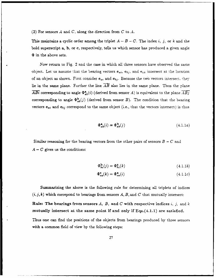
Summarizing the above is the following rule for determining all triplets of indices

(i, j, k) which correpond to bearings from sensors A, B, and C that mutually intersect:

Rule: The bearings from sensors A, B, and C with respective indices i, j, and k

mutually intersect at the same point if and only if Eqs.(4.1.1) are satisfied.

Thus one can find the positions of the objects from bearings produced by three sensors

with a common field of view by the following steps:

27

(1) For each sensor, transform the spherical coordinates for each data point to the angles

ID, as defined above.

(2) Search the sets of transformed angles, for those which satisfy Eqs. (4.1.1).

(3) Compute the intersection location for each triplet of bearings found in step 2.

This formulation permits the use of sorting or near-neighbor algorithms to find the

(i, j, k) corresponding to the same object. For example, to find those i and j satisfying

Eq.(4.1.1a), combine the set {qb(i)} coming from sensor .4 with the set {. b(j)} from

sensor B and then sort the entire set according to the values of these angles. Those angles

that are equal will be near neighbors in the sorted data array and finding all such pairs

will scale as N, the number of elements in the data structure. The next section describes

tests on various sorting and near-neighbor methods designed to find the data satisfying

Eqs.(4.1.1).

IV.2. Representative Algorithms and Tests

The algorithms and tests below account for errors in the bearing data due to finite sen-

sor resolution. Using the notation of the previous subsection, the three sensors A, B, and C

each produce bearing data transformed to the respective sets of angle pairs

Sensor A S, {(bW(i)',$ :(i)) = e,, i i = 1, 2,..., N,}

Sensor B Sb- {(Db ab(j), "(j)) = ebj =1, 2,..., Nb} (4.2.1)

SensorC: I k= 1, 2,..., No}

Given S., Sb, and S, as input, we will examine three algorithms for finding A

{(i,j,k) I such that e~i, eb&, eck satisfy Eq.(4.1.1)}. Thus A is the set of index triplets

that correspond to bearing vectors (one from each sensor) which intersect at the same

"point" (actually a region defined by the errors of the sensors). Given the bearing vectors

eai, ebi, and eck, one can directly compute the coordinates (X, y, z) of the potential object.

28

In the tests below, the quantity e denotes the characteristic error in the bearing data and

is a nonzero parameter.

IV.2.1. Parallel Matching Method

This method requires two one-dimensional sorts of the angle data and thus scales as

N in N. The term "parallel" here refers to the fact that the first two steps of the procedure

may be performed simultaneously on a minimum of two processors. Each of the major steps

of the procedure clearly contains similar searches whose lengths depends on the data sets.

The degree of parallellization will depend on the architecture of the particular computer

being used. The steps are as follows:

(1) Form a set, denoted Sob, by combining the angles #' b(i) E Sa with the angles 'b(j) E

Sb. Sort Sab and search outward from each element b(i) until the difference between

angle values exceeds e. This gives us the following subset of Sab which contains the solution

along with some false solutions:

Slb = {Sab(i) = {j I - e - Ib)(J) I b(i) ±e}li = 1,2,..., N, . (4.2.2)

(2) Perform the same operation with the angles ('(i) E Sa and Da(k) E S, in a set

denoted S.a. This gives us the subset of Sa:

Se ={ 1,2, ... , Na} (4.2.3)

(3) Now for each i, compare all Db(j) for j E S1b() with all -I)c(k) for k E S',(i). This

gives us the index triplets (i, j, k) that we seek.

These subsets S"b and S' should contain few bearings relative to the total number pro-

duced by a sensor, assuming that the sensor resolution ! is small relative to the average

interobject angular separation. In fact, we have assumed that the subsets S'b and S'a are

small relative to the binary logarithms of the number of elements in their parent sets Sab

and Sa. Otherwise the search for the correlated elements making up set Slb, for example,

would be done by constructing a binary tree containing all 6 b(i) E S. and then searching

the tree for the 1 .b(i) correlated with each Db(J) E Sb.

29

IV.2.2. The Monotonic Lagrangian Grid

The first step performed by the MLG method is to construct the set S'b exactly as inthe parallel matching method. For each i, the angles baab(i) E Sa and <Dabb(J) for j e Sb(i)

will then satisfy Eq.(4.1.1a) within the accuracy defined by e. Now take the set of their

counterpart angles

sab = i = 1, Na;j S'1,}4.2.4)

and combine these pairs with their counterpart pairs (Dc(k), (D'(k)) E Sc produced by

Sensor C in a two-dimensional MLG data structure:

A= S US, . (4.2.5)

The four angles satisfying the remaining two equations (4.1.1b) and (4.1.1c) should be

found in proximate pairs in A with one pair from each of the constituent sets in Eq.(4.2.5).

As noted above, when one searches small fixed-size neighborhoods of each point in the

MLG, the search is rapid but some of the correlations might be missed. Thus one first

finds a high percentage of the solutions, as shown by the data in Section IV.3. Then

one can repeat the procedure on a much smaller data set consisting of the remaining few

percent of the contact reports.

IV.2.3. A Shortcut Method

The value of this shortcut method lies in finding an acceptable percentage of possible

correlations rather than all of them while reducing the amount of computation significantly.

As in the previous methods, compute the set Sb defined by Eq.(4.2.4). For each i, find

the element j e Sb(i) which minimizes the deviation of ab(J) from 4"b(i). Then use the

triplet (Ca(i), D'(j), VR.(i)) as the solution. The philosophy behind this approach is that

ife ies small, then S.b will also be small. The best value of j will then have a high likelihood

of representing true correlations even without confirmation from sensor C. Thus, unlike the

30

MLG method which simply fails to report some correlations, the inaccuracy of the shortcut

method results from the fact that some false reports may be generated. Another variation

of this method might be to report every triplet (Z.ab(i), (bb(j), a(i)) as a correlation for

i= 1, 2,..., N, and j E Slb(i). This would ensure that in addition to some false reports.

a report would be generated for each of the real objects observed.

IV.3. Performance Results on a SUN-260 Workstation

The following tables provide relative performance information about the three al-

gorithms described. The tests took place on a SUN-260 Workstation, which is a scalar

machine. A floating point accelerator enhanced the speed. Table 3 displays execution

times and accuracy for N. = N 6 = N =_ N E {16K, 32K,..., 128K} objects, with each

test including an additional 10% spurious sensor readings. The value of e was chosen in

each test so that A(i), the average number of elements in Sb(i), was approximately

1.1. Table 4 presents the results of tests performed with fixed N = 16K and varying e

(or AAB(i)). This table reveals how the size of Slb(i) (as well as S'a(i)) for the paral-

lel matching method) affects the performance of each algorithm. Figure 4 displays the

execution-time breakdown of the parallel matching and MLG methods for N = 128K.

The data for all tests were obtained using a random number generator rand() which

produces a uniform distribution of values between 0 (inclusive) and 1. The first N values

for each sensor were generated as follows to ensure N correlations:

for i = 1 to N and i =j = k;

1:b(i) = rando; Ib (j) = & (i) drand( ) ;

1%(i) = rand); c 6 (k) = -V%(i) -rando. ;,'(j) = rando; c(k) = --- (j) =rand) e;

end;

A random number of spurious readings (amounting to around 10% of N) were then

added to each sensor and the order of the readings permuted so that eai, ebj, and eck

would not necessarily correlate for i = j = k . For simple statistical reasons, none of

31

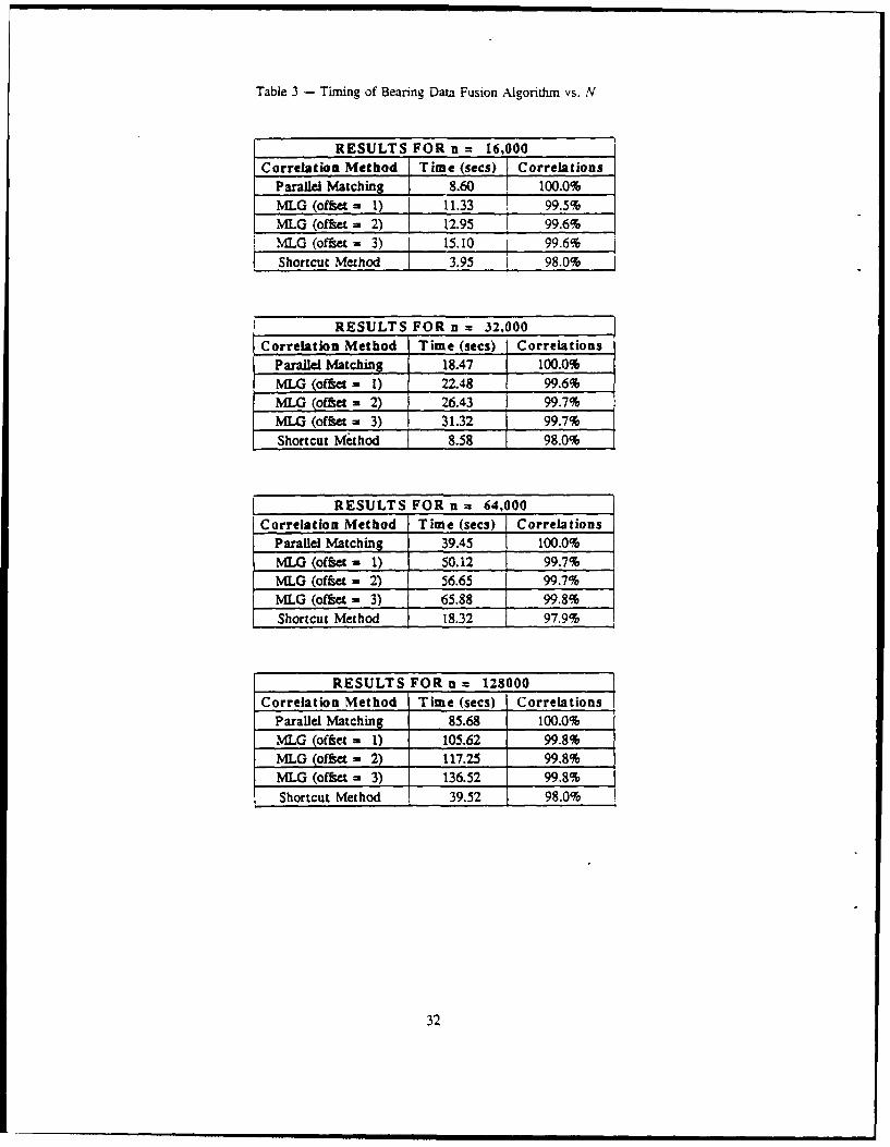
Table 3 - Timing of Bearing Data Fusion Algorithm vs. N

RESULTS FOR n = 16,000

Correlation Method Time (secs) CorrelationsParallel Matching 8.60 100.0%

MLG (oftset - 1) 11.33 99.5%

MLG (offet = 2) 12.95 99.6%

MLG (offer = 3) 15.10 99.6%

Shortcut Method 3.95 98.0%

RESULTS FOR n = 32.000

Correlation Method Time (secs) Correlations

Parallel Matching 18.47 100.0%

MLG (offset = 1) 22.48 99.6%MIO (ot'fit = 2) 26.43 99.7%

ML (offset = 3) 31.32 99.7%

Shortcut Method 8.58 98.0%

RESULTS FOR n = 64,000

Correlation Method Time (secs) Correlations

Parallel Matching 39.45 100.0%

MLG (offset = 1) 50.12 99.7%

MILG (offset = 2) 56.65 99.7%

MLG (offet = 3) 65.88 99.8%

Shortcut Method 18.32 97.9%

RESULTS FOR n = 128000

Correlation Method Time (secs) Correlations

Parallel Matching 85.68 100.0%

MLG (offet = 1) 105.62 99.8%

MLG (offet - 2) 117.25 99.8%

MLG (offset = 3) 136.52 99.8%

Shortcut Method 39.52 98.0%

32

Table 4 - Timing of Bearing Data Fusion Algorithm vs. Average Data Overlap

IAAI(i)I = 1.1 (n= 16000)Correlation Method Time (secs) Correlations

Parallel Matching 8.48 100.0%MLG (offset = 1) 11.15 99.4%Shortcut Method 3.98 98.0%

AS (i)I = 1.2 (n = 16000)

Correlation Method Time (secs) CorrelationsParallel Matching 8.79 100.0%

MLG (offset = 1) 11.34 99.4%Shortcut Method 3.99 95.8%

iAA S (;)I = 1.4 (n = 16000)Correlation Method Time (secs) Correlations

Parallel Matching 8.98 100.0%

MLG (offset = 1) 12.05 99.2%Shortcut Method 3.98 91.8%

IAAS (i) 1 1.8(n= 16000)

Correlation Method Time (secs) CorrelationsParallel Matching 9.33 100.0%

MLG (offset = 1) 13.08 99.0%Shortcut Method 3.97 84.2%

33

Execut ion-T ime BreakdownFor a= 128,000

105100 MOg search

90 . . . . . .

so bccb 6.1%75 Nag ......70 make-time65 ac ca

Time 60 46.7% match-time(secs) 55

so 46.M4540.. . . . . .. . . . . .3S3025 abba abba20 match-time nutch-time

15

0Mig Nkthod Parallel Nbtching Nkthod

Fig. 4 - Execution time breakdowns for the MLG and the Parallel Matching Method. The

notations "abba," "acca," and "bccb" correspond to steps 1, 2, and 3 of the latter

method, respectively.

34

the spurious readings produced false correlations in the tests performed. To produce false

correlations using these algorithms, much larger values of sensor error e or many more

contact reports would be required.

IV.4. Conclusions from Tests

If the accuracy of the shorcut method is acceptable for a particular application. hen

execution speed clearly makes it the method of choice; however, the high sensitivi7ty -o

measurement error (i.e., e) as target densities increase probably makes the shortcut method

impractical for use in a tracking system. This being the case, the parallel matching method

must be considered the superior algorithm on the SUN-260 because it is 100% accurate

and faster than the MLG method. Relative to brute force algorithms, either method is

much faster because of superior scaling with the size of the data set.

IV.5 Estimates of Performance on Other Hardware

Table 5 gives estimates of the performance of our multisensor fusion algorithm on

vanous machines, both sequential and parallel. The numbers are based on tests using the

MLG and on relative speeds of the computers. Under each machine name is the source

of the estimate. The timing estimates, shown correspond to 32.000 objects as viewed by

the three sensors. On various vector and parallel machines, the processing time is on the

order of I cpu second. The algorithm has thus reduced the complexity of the problem to

the point at which existing hardware can process the data rapidly for large numbers of

objects. With expected improvements in processing speed over the next few years, data

processing systems should easily meet the requirements for bearing to position conversion

on large numbers of objects with realistic values of sensor false alarm and error rates.

35

ocIr ct

r~O ~ ~ -0000

Qq w-r-

Z 0j

.5 0

m 0~ 0 r-

Cf 1~) .. o E =3

o-

36

V. Summary

This report has presented a preliminary view of the use of near-neighbor algorithms

in the processing of data on the bearings of the objects being observed. By assumption,

the sensors, such as infrared imaging devices, have provided either poor range information

or none at all. Our orientation has been toward correlation and tracking of large numbers

of high-speed objects. The purpose of the near-neighbor algorithms has been to organize

the data on a set of objects to permit rapid access of the data with a high correlation to

a given member of another set. The combinatorially inefficient "brute force" method, in

which all possible correlations between the two sets are considered, provides a baseline for

assessing the performance of the near-neighbor techniques. An interesting realization is

that, although the NN algorithms permit actual access to be superior, the overall cost of

the NN approach could be greater than brute force. This occurs, for example, if the NN

data structure must be set up too frequently. If the same data structure can be used for

groups of contact reports, then the NN algorithms should be much faster.

Some near-neighbor algorithms are also imperfect in that some near-neighbors, by

whatever definition of "nearness," might be missed if the search is too restricted. Clustering

algorithms can permit ambiguous assigranents of objects to particular clusters, for example.

The MLG algorithm can require searches of irregular regions of index space or of large

regions in order to insure finding all of the near neighbors. Tree-like searches of the MLG

data structure [6] might be necessary in some cases.

We have described the manner in which NN algorithms can be used in correlating

bearing data from a given sensor with a group of three-dimensional tracks. This is straight-

forward, and appropriate test results on data access in this situation are available' for the

MLG and Hockney's method.

The paper has also presented an example of a high-speed algorithm for converting

multisensor bearing data to positions for the objects within the region common to all of

the sensors. These algorithms will be superior to any brute force method for three or

37

more sensors, since the latter scales as N-, where m is the number of sensors, while our

algorithm is particularly suited for NN algorithms, which scale as N In N. The algorithm

also reduces the problem from determining the m-fold intersections of lines to the pairwise

equality of special angles. Thus the complexity is greatly reduced. Performance tests and

estimates indicate that the algorithms might already give existing hardware the capability

to satisfy the estimated processing requirements for situations in which large numbers of

objects are moving at high speeds. Certainly this will be the case in the future, given the

anticipated improvements in speed and memory of computer hardware.

VI. Acknowledgements

The authors acknowledge the support of the Strategic Defensive Initiative Organi-

zation and the Defense Advanced Research Projects Agency for the development of the

ideas presented in this paper. We also appreciate the effort of J. V. W. Reynders in pro-

gramming an initial version of the multisensor fusion algorithm on the Thinking Machines

Corporation Connection Machine.

38

References

1. J. A. Erbacher and B. Belkin, Tracker/Correlator Algorithm Design Document (Ball

Systems Engineering Division, Arlington, Virginia. 1983).

2. S. S. Blackman, Multiple-Target Tracking with Radar Applications (Artech

House, Dedhan, Massachusetts, 1986).

3. J. M. Picone, M. Zuniga, and J. Uhlmann, Tests of Gating Algorithms for Track-

ing of Multiple Objects I. Theory, Requirements, and Performance Measures, NRL

Memorandum Report, to be submitted (1989).

4. R. W. Hockney and J. W. Eastwood, Computer Simulation Using Particles,

McGraw-Hill, New York, chapter 8, pp. 267-309 (1981).

5. J. P. Boris, "A Vectorized 'Near Neighbors' Algorithm of Order N Using a Monotonic

Logical Grid", J. Comp. Phys. 66(1), PP. 1-20 (1986).

6. B. S. Kim and S. B. Park, "A Fast k-Nearest-Neighbor-Finding Algorithm Based

on the Ordered Partition", IEEE Transactions on Pattern Analysis and Machine

Intelligence, Vol. PAMI-8, No. 6, pp. 7 6 1-7 66 (1986).

7. R. Varad, private communication, MITRE Corp., Bedford, Massachusetts (1989).

39

Appendix: Details of Multisensor

Bearing-to-Position Conversion

For completeness, this appendix gives details on the transformation of the bearing

data from each sensor to new angles denoted by D. Figure 5 returns to the example used

previously (Fig. 3) for a bearing vector ebj corresponding to Sensor B. Figure 5b shows

that the angle 'c(j) can be computed from the unit normals to the plahe of the sensors

and the plane defined by ebc (the vector from Sensor B to Sensor C) and the bearing vector

ebi.

First define the unit vector , perpendicular to the plane of the sensors. If the site

producing the bearing vector is I E {A, B, C}, then we define the values of I - 1 and 1 4- 1

by the preceding and following sensor indices in the appropriate cyclic permutation of the

sequenceA-B--C. For example, ifI = B, then I-1 I A and I+1 - C. Then the

desired unit vector is the vector cross product

e(+l) x e(I-1), (A.1)

" ej1+1) x e(I-1)1"

In our example with I = B, this becomes

/34= eb, x eab(A2jebc x eabi

The perpendicular to the plane BCj is

- eb, x eb (4.3)lebi x ebcj

The angle Db (j) then satisfies the equations

sin ,p¢(j) M (f3bc(j) x 0.) ebc (A.4a)

coOS'b'c(j) M &(j)" -, ), (A.4b)

41

%WOO)

__ .77-

C1 . 0,0u

(A A

.-- , 4

~ : -o

42~

in which the centered dot (.) signifies a scalar product. Figure 5c shows the definition of

the second angle -'P (j) corresponding to the bearing vector ebi. This is the angle between

the plane of the sensors and the plane defined by the line joining sensors A and B and the

bearing vector ebi. By convention (Section IV.A), the observer's line of sight runs from

sensor A toward sensor B, producing the view shown in Fig. .5c. A cyclic permutation of

the subscripts A - B - C will define the angles corresponding to bearing vectors produced

by sensors A and B.

The remaining question is that of transforming the uncertainty (o, Ao) to uncer-

tainties in the new angles . Again consider the angle 'Ib'(j) and the bearing vector

ebi =- (Ob(j), Ob(i)). Define the right-handed coordinate axes (visualize with Fig.Sb)

x ebc

y e .b (A.5)

Z=

Then, if the subscripts on the bearing angles are dropped for convenience, the important

unit vectors are

ebj= (sin 0 cos 0, sin 0 sin b, cosO)

, (0, 0, 1) (A.6)

ebc = (1, 0,0)

Equation(A.3) then gives us

O3bc(j) = G (0, cos 8, - sin 8 sin 6) , (A.7)

where

G = (cos20 + sin 2 Osin2 2 (A.S)

Equations(A.4) then become

43

sin 0Db(j) = G cos 9

cos 4 b(j) = -G sin0sinO

Equations (A.7)-(A.9) show that the error in the new angles varies with the bearing vector

eb,. The new angles themselves can become undefined for pathological cases in which the

three bearing vectors are not distinct or for which the bearing vectors He close to -,he plane

of the sensors. An example would be an object lying along or near the line eh,. in which

case (0, 0) = (Z, 0). At the other extreme, for 0 = mir, where m is an integer, and variable

0, the error in PDb(j) is A2 - A92. The general equations for the error become unwieldy

because of the normalization factor G. A detailed examination is necessary to determine

the ranges of bearing vectors for which their intersections yield useful position data. Since

our method is equivalent to the brute force ("intersection") approach, the range of validity

will be the same. One method of determining this range in the context of our method is

to use the equations in this appendix in conjunction with a limit on the allowable size of

the errors in the angles (. An example of such a constraint is

(aA b(j))2 < (A8 + ,O). (4.10)

44