Determination of reaction coordinates via locallyscaled di!usion mapMary A. Rohrdanz !, Wenwei Zheng ! , Mauro Maggioni † and Cecilia Clementi !

!Department of Chemistry, Rice University, Houston, TX 77005 , and †Department of Mathematics, Department of Computer Science, Duke University, Durham, NC 27708

Submitted to Proceedings of the National Academy of Sciences of the United States of America

We present a multiscale method for the determination of collectivereaction coordinates for macromolecular dynamics by combining tworecently developed mathematical techniques: di!usion map and thedetermination of local intrinsic dimensionality of large data sets. Ourmethod is mathematically rigorous and accounts for the fact that thee!ective local dimensionality changes from region to region in thespace of molecular configurations. To illustrate the approach, wepresent results for two model systems: all-atom alanine dipeptideand coarse-grained SH3. We verify that the coordinates emergingfrom our method capture the essential dynamics by calculating tran-sition rates via Kramers escape rate.

reaction coordinates | di!usion map | alanine dipeptide | molecular dynamics

| coarse-grained simulation

Abbreviations: SH3, src homology 3 domain; MD, molecular dynamics; 1stDC , first

di!usion map coordinate; 2nd

DC , second di!usion map coordinate

The pursuit of collective reaction coordinates for macro-molecular dynamics is of great interest in molecular bio-

physics, as such coordinates are crucial for extracting mean-ingful information from the large volume of data routinelyproduced by macromolecular simulations (e.g., molecular dy-namics (MD)). In the last few years, a number of groups haveworked toward defining good collective coordinates for chem-ical and biological processes, and di!erent approaches havebeen proposed, e.g. [1, 2, 3, 4, 5, 6, 7, 8].

Most of the proposed methods are based on the hypothesisthat macromolecular motion over a long time scale can be es-sentially described in terms of a few collective variables. Theso-called “energy landscape theory” of protein folding [9] isone example. This working assumption has been empiricallyverified for a number of di!erent systems, e.g. [7, 10, 11],and motivates the definition of empirical coordinates, oftenbased on physical intuition, with which to study the system’scollective dynamics and identify (meta-)stable states.

This intuition can be interpreted geometrically: the distri-bution of states in configurational space is highly concentratedaround a set, M, of much lower dimensionality than the ambi-ent configurational space. The analysis of such sets embeddedin very high-dimensional spaces is an area of mathematicalresearch that has become a necessity in a broad range of dif-ferent disciplines (e.g., genomics, imaging, machine learning–see [12, 13, 14, 15], and references therein). However, therehas been only a small amount of work to rigorously addressthe estimation of the number of independent variables neededto describe the configurational space of a macromolecular pro-cess [3, 16, 4], that is, to estimate its e!ective dimensionality.The problem is complicated by the fact that any definitionof an intrinsic dimension for these processes requires multiplescales: we expect the number of collective variables neededto describe macromolecular dynamics (i.e. the geometry ofM) to change as a function of time and space. In addition, ifwe describe the long-timescale dynamics in terms of a smallnumber of “slow” variables, we implicitly assume that the re-maining degrees of freedom contribute as “noise” around thelow-dimensional manifold, M. Previous attempts (e.g., [3])

have been limited to consideration of only the longest timescales, and have not taken noise into account.

To address all these issues, we propose a novel multiscaleframework that provides collective coordinates over di!erenttimescales and combines the characterization of the globalmanifold, M, with the notion of local scale, that is, the min-imum length scale above the noise such that the intrinsic ge-ometric properties of M can be captured and characterizedlocally. To obtain global observables, these local models are“glued” together to form an overall consistent picture.

If an infinite amount of data were sampled from a noiselessM, the local scale could be chosen infinitesimally small, trivi-alizing the problem; however we are interested in macromolec-ular simulations, which have limited data clustered around anoisy M. In such situations the local scale must be chosenmore carefully. It must be both larger than the scale of thenoise and large enough to provide adequate sampling for es-timation of geometric properties of M at that scale, whilesimultaneously smaller than the curvature of M. These con-flicting requirements make this problem hard, but recent re-sults provide a near-optimal solution, with associated e"cientalgorithms [17].

The approach we propose is mathematically rigorous, asit builds upon two recently developed mathematical tech-niques for noisy data sets: multiscale analysis of di!usion pro-cesses [18, 19] and estimation of intrinsic dimension [17]. Here,the “noisy data set” is a collection of configurations extractedfrom a molecular dynamics simulation, and the estimation ofthe local dimension around each configuration allows for thedetermination of a local length scale in configuration space.The local length scale is then used as input to characterizea global di!usion process by using a generalized version ofthe recently proposed di!usion map approach [18, 20, 21]. Assuggested by recent literature [18, 22, 23], we use the di!usionmap eigenfunctions as global coordinates.

We apply our framework to characterize the dynamics oftwo very di!erent molecular systems (an all-atom model ofalanine dipeptide, and a coarse-grained model of the src ho-mology 3 domain protein (SH3)), and show that the dynam-ics of these systems can be globally represented by a low-dimensional set; however, the intrinsic dimension of the setvaries from region to region, and this heterogeneity needs tobe accounted for in defining the global coordinates. In thissense, our multiscale approach is in spirit similar to a “renor-

Reserved for Publication Footnotes

www.pnas.org/cgi/doi/10.1073/pnas.0709640104 PNAS Issue Date Volume Issue Number 1–8

malization” of di!erent regions of the configurational spaceaccording to each region’s local scale and geometric structure;a global di!usion process across these “renormalized” regionsis then extracted.

We show that the collective coordinates emerging fromthis approach capture the overall dynamics of the systemsunder consideration; this assertion is quantified by using theextracted coordinates to correctly reproduce the rate of thedi!usion process across the barriers separating the di!erentfree energy minima for both systems considered.

Di!usion mapOur multiscale method builds on and complements the idea of“di!usion maps”, originally proposed by [18] and applied invarious contexts, such as machine learning tasks [15, 24] andmanifold parametrization [22].

We briefly review here the most relevant features of thedi!usion map as it applies to our setting (see also SupportingInformation sections 1, 2, and 3), and refer to the literature(e.g., [23]) for details. The central idea is that for dynamicswhich are approximately di!usive, and for which there is aseparation of timescales between one (or a few) slow relax-ation process(es) and the remaining faster ones, the eigen-functions of the Fokker-Planck operator associated with theslowest timescales can be used to define a set of collectivecoordinates to describe long-time dynamics.

For a system with a given potential energy function, E(x),at constant temperature, T , and in the limit of high friction,the Fokker-Planck equation governs the temporal evolutionof the probability distribution, p(x, t), at any configuration,x ! R

N , of the system:

!p!t

= "N!

i

!!xi

"

1"

!!xi

+!E!xi

#

p = "HFPp, [1]

where " = 1/(kBT ), and kB is Boltzmann’s constant. Underrather general conditions, the operator HFP, which acts on aninfinite-dimensional space of probability distributions, has adiscrete eigenspectrum of non-negative eigenvalues, #i, with#0 = 0 < #1 # #2 # . . . , and corresponding eigenfunctions,$i(x). Formally (and rigorously in an appropriate metric thatdepends on various assumptions on HFP), the general solutionof the Fokker-Planck equation is:

p(x, t) = $0(x) +"!

i=1

ci$i(x)e#!it [2]

where the coe"cients, ci, are determined by the initial distri-bution, p(x, t = 0). The eigenfunction $0(x) is the Boltz-mann distribution, approached by any initial distributionwhen t $ 1/#1.

For systems with one (or a few) slow process(es) domi-nating the dynamics (such as the crossing of a free energybarrier), the eigenspectrum will present a gap, i.e. #k+1 $ #k

for some k, and the evolution of the probability distributiontoward equilibrium may be approximated as

p(x, t) = $0(x) +k

!

i=1

ci$i(x)e#!it, [3]

at least at time scales t $ 1/#k+1. Therefore, in these situa-tions it is “natural” to define the normalized eigenfunctions,$i(x)/$0(x), as collective coordinates1[23]. The geometricintuition is that the Boltzmann distribution, $0, is a mea-sure essentially supported on a k-dimensional set, M, withk % N , and at least when this set is a (not necessarily smooth)

manifold, the eigenfunctions above provide quantitatively andprovably good coordinate systems [22].

An e"cient numerical method to approximate these firstfew eigenfunctions and associated eigenvalues by using onlysamples of the equilibrium distribution has been recently pro-posed [23]. In principle this procedure can be applied to ob-tain collective coordinates from a set of molecular configu-rations extracted from a standard MD simulation (as we dobelow). The approach involves defining a weighted graph, G,on the simulation data {xi}, and determining the first feweigenvalues and eigenvectors of a random walk on the graph.The weights are related to the transition probability betweenconfigurations, and will be larger for configurations that aresimilar in structure. Here we measure similarity by the rootmean square deviation (RMSD) between structures (as op-posed to Euclidean distance used in [23]), in order to quotientout irrelevant translational and rotational degrees of freedom.The transition probability between any two structures is basedon the kernel,

K(xi,xj) = e#

||xi"xj ||2

2!i!j , [4]

where xi and xj represent two molecular configurations, and||xi " xj || is their RMSD. An appropriate renormalization ofK, described in the Supporting Information section 2, leadsto a random walk, P , on {xi} whose eigenfunctions approx-imate those in Equation [2]. The local scale parameter, %i,appearing in Equation [4] can be interpreted as the distancearound the configuration xi at which the motion can be con-sidered locally “flat”, i.e. can be well-approximated by thelow-dimensional hyperplane tangent at xi to the manifold Mon which the Boltzmann distribution is e!ectively supported.

In previous applications of di!usion maps, %i has alwaysbeen chosen equal to a constant value, %, independently of xi.Little is known about the choice of this crucial parameter,with theoretical results providing only some guidance in theasymptotic regime when the number of configurations is verylarge (at least exponential in the intrinsic dimension of the ef-fective configuration space), and often ad-hoc techniques areused in practice. We propose a principled way of selecting thelocal scale parameter; we show below that the dependency of%i on xi plays a fundamental role in the definition of collec-tive coordinates, and in the application of di!usion map ingeneral.

Determination of local dimension and scaleThe information about the local environment of each config-uration, xi, is captured by the local scale parameter, %i. Asdiscussed above, in previous applications of the di!usion mapmethod the parameter % is taken to be a constant [18, 23]. Ifthe data sample is dense and lies on a smooth, non-noisy, low-dimensional manifold, the choice of % is not critical to the nu-merical estimation of the Fokker-Planck eigenfunctions–usinga constant value yields meaningful results (as the number ofsamples grows, the estimated generator of the di!usion con-verges to the true generator of the Fokker-Planck equation).

However a data set of macromolecular configurations fromMD simulations has highly variable density (due to the prop-erties of the Boltzmann distribution), is very noisy (with thecharacteristics of the noise changing with the region of con-figurational space), and it is not infinitely dense. In such asituation, if the parameter % is selected too small, for exam-ple comparable to the scale of the noise, the results will be

1The functions "i(x)/"0(x) are the eigenfunctions of the backward Fokker-Planck opera-tor [23],as explained in the Supplementary Information, section 1.

2 www.pnas.org/cgi/doi/10.1073/pnas.0709640104 Footline Author

corrupted because the “locally flat” region will correspond tothat of the noise rather than that of the actual data. On theother hand, if % is too large, large regions of the system willbe considered artificially flat, again corrupting the results.

In practice one observes that if a uniform value of % isused for every configuration in a noisy sample of macromolec-ular dynamics, the eigenspectrum obtained from the di!usionmap analysis is strongly dependent on the selected value of%, and no straightforward interpretation of the data can beobtained. Examples on the application of di!usion map withconstant % to both systems considered here are discussed inthe Supporting Information section 5.

The changes in density, noise shape, and geometry of Msuggest that a variable value of % is more natural. For exam-ple, one can intuitively guess that at the top of a free energysaddle-point between two minima the e!ective number of de-grees of freedom needed to describe the motion locally (thatis, the local dimension) may be much smaller than at the bot-tom of the free energy minima. In order to obtain results withclear physical meaning, we determine the local dimension andlocal scale parameter, %i, for each data point, xi, of the sam-ple through an analysis of the geometry of the local manifoldaround xi.

Inspired by the results presented in [17], we define a math-ematically robust method for determining the intrinsic dimen-sion and local scale associated with each configuration in ournoisy data set. In essence, as the local scale parameter, %i,indicates the (unknown) lengthscale at which M can be wellapproximated by its (unknown) tangent hyperplane at xi, weobtain an estimate of %i by performing linear dimensionalityreduction, such as Principal Component Analysis (PCA), overincreasingly large neighborhoods of xi. It is shown in [17] thatunder very general assumptions on the geometry of M, thedensity of points, and the noise, such technique leads to robustidentification of the local scale and intrinsic dimension aroundany point on M. Moreover, this technique requires a numberof samples {xi} which is only linear in the intrinsic dimen-sion, k, of M, instead of exponential in k, and independentof the large ambient dimension. Because we are using RMSDbetween samples and not Euclidean distance, we kernelize thetechniques of [17] in order to make them applicable to thissetting. Technical details on this method for the determina-tion of %i are provided in the Supporting Information section4. While other algorithmic approaches for estimating the in-trinsic dimension of embedded manifolds exist, each of themtypically present one or more of the following deficiencies: re-quiring a large sample size, high sensitivity to noise, assumingsmoothness of the underlying manifold, assuming constant di-mension, they do not analyze the geometry at multiple scales,and/or do not identify a characteristic lengthscale. Theoremssupporting such algorithms, when they exist, typically assumea sample size going to infinity, and no noise. We refer thereader to [17] for an in-depth discussion, comparisons and ref-erences.

ApplicationsWe apply the locally scaled di!usion map approach to twotest systems: all-atom alanine dipeptide in implicit water, andcoarse-grained SH3. To quantify our assertion that the di!u-sion map coordinates correctly reproduce the overall long-timedynamics, for both systems we define a free energy as a func-tion of the first di!usion coordinate, and estimate the rates forthe di!usion between free energy minima by using Kramersexpression [25] for the escape rate of a system moving over a

2n

d D

C

!1.5 !1 !0.5 0 0.5

!4

!3

!2

!1

0

Fre

e E

ner

gy

(k

cal/

mo

l)

0

2

4

6

!1.5 !1 !0.5 0 0.50

2

4

1st

DC

Fre

e E

ner

gy

(k

cal/

mo

l)

C5

P!!

"R

"P

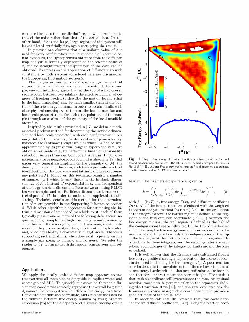
Fig. 1. Top: Free energy of alanine dipeptide as a function of the first andsecond di!usion map coordinates. The labels for the minima correspond to those inFig. 3 of [4]. Bottom: Free energy profile along the first di!usion map coordinate.The Kramers rate along 1stDC is shown in Table 1.

barrier. The Kramers escape rate is given by

k =

"$

barrier

e#F (x)

D(x)dx

$

well

e##F (x#)dx$

##1

, [5]

with " = (kBT )#1, free energy F (x), and di!usion coe"cient

D(x). All of the free energies are calculated with the weightedhistogram analysis method (WHAM) [26]. In the evaluationof the integrals above, the barrier region is defined as the seg-ment of the first di!usion coordinate (1stDC ) between thefree energy minima; the well region is defined as the half ofthe configurational space delimited by the top of the barrierand containing the free energy minimum corresponding to thereactant state. In practice, only the configurations at the topof the barrier, or at the bottom of a minimum will significantlycontribute to these integrals, and the resulting rates are veryrobust upon changes of the integration limits around the onesso defined.

It is well known that the Kramers rate calculated from afree energy profile is strongly dependent on the choice of coor-dinates used in defining the free energy [27]. A poor reactioncoordinate tends to convolute motion directed over the top ofa free energy barrier with motion perpendicular to the barrier,and therefore underestimates the barrier height. The result isthat such a coordinate will overestimate the rate. An optimalreaction coordinate is perpendicular to the separatrix defin-ing the transition state [11], and the rate evaluated via theKramers expression along such a coordinate should provide agood estimate of the actual rate.

In order to calculate the Kramers rate, the coordinate-dependent di!usion coe"cient, D(x), along the reaction coor-

Footline Author PNAS Issue Date Volume Issue Number 3

Fig. 3. The raw molecular configuration data obtained from a long MD trajectoryof alanine dipeptide are plotted as a function of the 1stDC and the dihedral angle! (left panel), and the dihedral angles " and ! (right panel). In both panels, thecolor indicates di!erent values of the 1stDC , as indicated by the colorscale at thetop of the figure. The mapping between the 1stDC and the dihedral angle ! is ap-proximately one-to-one. The labels for the states, C5, P%, !R, and !P correspondto those of the free energy minima shown in Fig. 1.

dinates is required. This was obtained by using the Bayesiananalysis method presented in [28] to extract D(x) from theMD simulation data. Details on our determination of the dif-fusion coe"cients are available in the Supporting Informationsection 6.

Alanine dipeptide.Alanine dipeptide is a typical testbed forcollective dynamics studies. Although the molecule consistsof 22 atoms, multiple steric constraints e!ectively reduce theconfiguration space to two dimensions under standard condi-tions. The two dimensions of choice are the dihedral angles,# and $. As the two angles are a priori known, this systemrepresents an ideal case to test our approach.

The MD data is obtained from a 300 K simulation withthe AMBER99 force field in implicit water. Configurationscollected every 0.1 ps during a 20,000 ps simulation are usedas input to the local scale determination and di!usion mapcalculation. The free energy as a function of the first and sec-ond di!usion map coordinates (1stDC and 2ndDC) is shownin the top panel of Fig. 1.

It is important to emphasize a few points about the trajec-tory data. A much smaller data set can be used to define thedi!usion coordinates by applying our locally scaled di!usionmap approach. The di!usion coordinates and the free energymap as a function of these coordinates constructed by using asmaller set of 10,000 configurations are indistinguishable fromthe corresponding quantities obtained on the larger sample,and can be obtained in a day of computer time on a single-core workstation. The reason for using such a large data sethere is twofold: to test the robustness of the results obtainedon smaller samples, and to provide adequate statistics for thecalculation of the di!usion coe"cients from Bayesian analysis[28] from a single long trajectory. Alternatively, if a smallerdata sample is used, the di!usion coe"cients at a positionx along the 1stDC could be estimated by using many inde-pendent, short simulations starting from di!erent molecularconfigurations at position x [28].

Previous studies of this system show four minima when thefree energy is plotted as a function of # and $ (see, for exam-ple, Fig. 3 of [4]). These same minima are also present in thedi!usion map coordinates. One of the features of the di!usionmap calculation is that each of the di!usion map coordinates(DCs) corresponds to a di!erent time scale in the system’s dy-namics, and therefore usually separates two metastable states.The eigenvalue spectrum of this system (see Fig. S1) presentsa gap between the first and second nontrivial eigenvalues, indi-cating that there is one process dominating the long timescaledynamics. In particular, the first nontrivial eigenvalue and as-sociated 1stDC correspond to the isomerization connecting thetwo pairs of minima C5–P%, and &P –&R, as shown in Fig. 3.The 2ndDC , that is, the second slowest timescale, correspondsto the di!usion from the P% minimum to the C5 minimum.The 3rdDC corresponds to transitions between the &P and &R

minima. The free energy as a function of 1stDC and 3rdDC isshown in Fig. S2; the analogous of Fig. 3 for 2ndDC and3rdDC is shown in Fig. S3.

We quantify the assertion that the 1stDC captures the es-sential dynamics of the isomerization process between C5–P%

and &R–&P by calculating the Kramers rate (Equation [5]),with free energy and di!usion coe"cients calculated as a func-tion of the 1stDC . The results are reported in Table 1, alongwith the rate calculated using free energy and di!usion coef-ficients as a function of the dihedral angle, $. The di!usioncoe"cients along each coordinate are obtained from Bayesiananalysis [28], as detailed in the Supporting Information sec-tion 6. Both the rate along the 1stDC and $ are in excellentagreement with the rate extracted directly from simulation,suggesting that both the 1stDC and $ are good reaction co-ordinates for this transition. Indeed, the 1stDC and $ arestrongly correlated, as shown in Fig. 3.

We have performed these same calculations using a con-stant value of %, and find the constant-' calculations unable tocapture the essential dynamics of this system. The constant-'results are detailed in the Supporting Information section 5,and Figs. S10, S11, and S12.

The relationship between 2ndDC and 3rdDC with the di-hedral angles, # and $, are presented in Fig. S3; informationon the local dimension and local scale for each configurationin our data set are shown in Fig. S6.

Table 1. Alanine dipeptide isomerization rates(ps#1)a

Coordinate C5, P% & &R &P &R &P & C5, P%

From simulationb 0.023 0.0471stDC 0.023 ± 0.001 0.048 ± 0.003$ 0.020 ± 0.001 0.040 ± 0.003aSee the Supporting Information for details on the error analysis.

bStandard deviation for simulation rates are of order 10"4 ps"1

Coarse-grained model of SH3.The folding dynamics of the57-residue protein domain SH3 has been well characterizedboth by simulation studies [29, 30, 31] and wet-lab experi-ments [32]. This protein is known to fold in a two-state man-ner, that is, only the unfolded or folded states are significantlypopulated near the folding transition temperature, Tf . Thefolding/unfolding process is known to be the longest timescalein the protein dynamics, and corresponds to di!usion over thefree energy barrier separating the folded and unfolded states.Previous studies have shown that the free energy landscape

4 www.pnas.org/cgi/doi/10.1073/pnas.0709640104 Footline Author

of SH3 can be well approximated by a few global coordinates,either empirically defined [29, 33], or obtained through non-linear dimension reduction techniques [3, 16]. As with alaninedipeptide, previous work on this system makes it an ideal testcase for our approach.

We apply our method to simulation data obtained withthe coarse-grained model of SH3 described in [34]. MD sim-ulations were performed in GROMACS near Tf , and config-urations collected every 5 ps during a 500,000 ps run. These100,000 configurations were used as input to the local scaledetermination and di!usion map calculation. As with ala-nine, the trajectory used here is at least 10 times longer thanwhat needed to obtain reliable results with our approach; asimilar set of DCs and free energy map is obtained with only10,000 configurations. The reason for such a large data setis the determination of the di!usion coe"cients from a singletrajectory, as discussed above.

2n

d D

C

!4

!2

0

2

Free Energy (kcal/mol)

0 4 8

!1.5 !1 !0.5 0 0.5 10

2

4

6

1st

DC

Fre

e E

ner

gy

(k

cal/

mo

l)

Fig. 2. Top: Free energy of the coarse-grained SH3 model as a function ofthe first and second DCs. Bottom: Free energy profile along the 1stDC . TheKramers rate along 1stDC is shown in Table 2.

The large gap between the first and second nontrivialeigenvalues in the di!usion map eigenspectrum of SH3 (illus-trated in Fig. S1) indicates a clear separation of time scale,with one slow di!usion process dominating the long timescaledynamics.

The free energy as a function of the first two DCs is shownin the top panel of Fig. 2, and the free energy profile alongthe 1stDC is shown in the bottom panel. The free energyminimum on the right corresponds to the folded state, andthe minimum on the left is the unfolded state. These min-ima appear well separated along the 1stDC , indicating thatthe folding/unfolding transition is the longest timescale of thesystem dynamics. Table 2 presents the Kramers rates calcu-lated by using the 1stDC to define the free energy and thedi!usion coe"cients; the rates are compared with the valuesobtained when other coordinates are used, namely the RMSD

Fig. 5. The raw molecular configuration data points, collected during a long tra-jectory of the coarse grained SH3 model, are plotted as a function of the 1stDC andRMSD with respect to the native state (left), and as a function of the fraction of nativecontacts, Q, and RMSD (right). The points are colored according to their 1stDC .The coloration shows the mapping between 1stDC and RMSD to be approximatelyone-to-one.

with respect to the native structure, and the fraction of nativecontacts, Q. The RMSD distance produces a rate comparableto the values obtained with the 1stDC ; indeed, the 1stDC andRMSD appear to be strongly correlated, as shown in Fig. 5.The Pearson correlation coe"cient, r, of 1stDC and RMSDcalculated on the 100,000 data set is r = 0.97; the correla-tion of 1stDC and Q is also high (r = 0.93), although nothigh enough to be able to accurately reproduce the proteinfolding/unfolding rate.

In order to understand the physical meaning of the1stDC and 2ndDC in the dynamics of the SH3 model, we com-pute the probability of contact formation for all the pairs ofresidues in the protein, along the 1stDC and 2ndDC . For eachcontact we compute the Spearman rank and Pearson correla-tion coe"cient between the 1stDC and the probability of for-mation as a function of the 1stDC, and between the 2ndDC andthe probability of formation along the 2ndDC. Fig. 4 displaysthe contacts with both a Spearman rank and Pearson correla-tion coe"cient larger than 0.8 and a probability of formationlarger than 0.1, for the 1stDC (lower contact map), and the2ndDC (upper contact map). The contacts shown in blue inthe lower right of Fig. 4 tend to form as the 1stDC increases.Indeed, these are the native contacts, confirming that the mo-tion along 1stDC corresponds to the folding process. In theupper left of Fig. 4, the contacts in red tend to form as the2ndDC increases. Interestingly, these contacts include the setof non-native contacts involved in the formation of a non-specific hydrophobic nucleus (circled in red in the figure), thathave been previously determined to be important in the fold-ing mechanism of SH3, both experimentally [35] and in sim-ulations (see Fig. 4 of [34] for comparison). This cluster ofnon-native contacts is the only cluster of contacts with botha Spearman rank and Pearson correlation coe"cient largerthan 0.9. Fig. S4 in the Supporting Information shows thatthe 2ndDC presents a maximum at the transition state, anddecreases moving away from the transition state toward boththe native and non-native states. Taken together these resultsindicate that the second slowest time scale in the folding of

Footline Author PNAS Issue Date Volume Issue Number 5

SH3 corresponds to the formation of a folding nucleus involv-ing this set of non-native contacts, which are formed at thetransition state but not formed in the unfolded and foldedstates.

0 5 10 15 20 25 30 35 40 45 50 5505

10152025303540455055

1.00.8

0.8

0.9

0.9

1.0

Fig. 4. Correlation of SH3 probability of contact formation with 1stDC (lowerright) and 2ndDC (upper left). Native contacts are marked by a black dot. Thecolored contacts are those with both a Spearman rank and Pearson correlation coe"-cient greater than 0.8, and an probability for forming greater than 0.1. The contactsshown in blue in the contact map below the diagonal are correlated with the 1stDC ,while those shown in red above the diagonal are correlated with the 2ndDC. Di!erentshades of red or blue indicate di!erent values of the Pearson correlation coe"cient,as indicated in the colorscale on the right.

It is important to point out that the analysis of the correla-tion of the first few DCs with the contact probabilities (and/orother parameters, like the RMSD from the native structure, orthe parameter Q) can be used in general with any other foldingmodel, to identify the physical quantities that are associatedwith the di!erent timescales in the di!usion dynamics.

Table 2. SH3 folding rates (ps#1).a

Coordinate Folded & Unfolded Unfolded & Folded

From simulation (4.4 ± 0.4) ' 10#5 (6.4 ± 0.4) ' 10#5

1stDC (6.9 ± 0.8) ' 10#5 (8.0 ± 0.9) ' 10#5

RMSDb (9 ± 1) ' 10#5 (12 ± 1) ' 10#5

Q (3.1 ± 0.5) ' 10#4 (3.7 ± 0.7) ' 10#4

aSee the Supporting Information for details on error analysis.

bRMSD with respect to the native structure.

ConclusionsWe propose a multiscale, mathematically rigorous approachfor extracting collective coordinates from a configurationalsample of macromolecular motion. The approach is basedon the determination, at each point of the sample, of thelength scale at which the dynamics can be considered locallylinear; this position-dependent length scale is then used tolocally “renormalize” the kernel of the transition probabilitybetween each pair of configurations; a di!usion map is thenconstructed on the global di!usion process. We have shownthat, for systems with a separation of time scales in which theslowest timescale is associated with the di!usion over a freeenergy barrier, the first di!usion map coordinate can be usedas a reaction coordinate. Reaction rates computed by usingKramers rate expression along the first di!usion coordinateare in remarkable agreement with the rates measured directlyfrom simulation data.

The analysis of the correlation of first few di!usion mapcoordinates with physical observables reveals the mechanismsassociated with the di!erent timescales in macromolecular dy-namics. For the folding of a coarse-grained model of SH3, wefind that the collective dynamics associated with the secondtimescale (thus motion along the second di!usion coordinate)corresponds to the formation of a set of non-native contactsat the core of the protein.

At the best of our knowledge, this is the first timerigourous mathematical techniques in multiscale geometrictheory have been developed for the analysis of macromolecu-lar dynamics data. The data are viewed as noisy point cloudsin very high dimensional spaces, that are intrinsically low di-mensional. We think this is a first step in the direction ofquantifying and exploiting geometric properties of trajecto-ries arising from MD simulations.

We believe the approach presented provides a powerfultool that can be used in general to understand the collectiveprocesses at play in complex di!usion reactions over a spec-trum of di!erent time and length scales, when a sample of theequilibrium distribution is available.

ACKNOWLEDGMENTS. This work was supported by NSF (CDI-type I grant0835824 to C.C. and 0835712 to M.M., NSF CAREER award CHE-0349303 to C.C.,and NSF CAREER award DMS-0650413 to M.M.), the Welch Foundation (C-1570to C.C.), and the Sloan Foundation (to M.M.). Simulations and other computa-tions were performed on the following shared resources at Rice University: the RiceComputational Research Clusters funded by NSF under grant CNS-0421109 and inpartnership between Rice University, AMD and Cray; the Cyberinfrastructure for Com-putational Research funded by NSF under grant CNS-0821727; the Shared UniversityGrid at Rice University funded by NSF under grant EIA-0216467 and in partnershipbetween Rice University, Sun Microsystems, and Sigma Solutions, Inc.; and a 2010IBM Shared University Research (SUR) Award on IBM’s Power7 high performancecluster (BlueBioU) to Rice University as part of IBM’s Smarter Planet Initiatives inLife Science/Healthcare and in collaboration with the Texas Medical Center partners,with additional contributions from IBM, CISCO, Qlogic and Adaptive Computing.

6 www.pnas.org/cgi/doi/10.1073/pnas.0709640104 Footline Author

1. Best RB and Hummer G (2005) Reaction coordinates and rates from transition paths.

P Natl Acad Sci USA 102:6732–6737.

2. Peters B and Trout BL (2006) Obtaining reaction coordinates by likelihood maximiza-

tion. J Chem Phys 125:054108.

3. Das P, Moll M, Stamati H, Kavraki LE and Clementi C (2006) Low-dimensional, free-

energy landscapes of protein-folding reactions by nonlinear dimensionality reduction.

P Natl Acad Sci USA 103:9885–9890.

4. Stamati H, Clementi C and Kavraki L (2010) Application of nonlinear dimensionality

reduction to characterize the conformational landscape of small peptides. Proteins:

Structure, Function, and Bioinformatics 78:223–235.

5. Dellago C, Bolhuis P and Chandler D (1998) E"cient transition path sampling: Ap-

plication to Lennard-Jones cluster rearrangements. J Chem Phys 108:9236–9245.

6. E W, Ren W and Vanden-Eijnden E (2002) String method for the study of rare events.

Phys Rev B 66:052301.

7. Qi B, Mu! S, Caflisch A and Dinner AR (2010) Extracting physically intuitive re-

action coordinates from transition networks of a "-sheet miniprotein. J Phys Chem

114:6979–6989.

8. Plotkin S and Wolynes P (1998) Non-Markovian configurational di!usion and reaction

coordinates for protein folding. Phys Rev Lett 80:5015–5018.

9. Onuchic J, Luthey-Schulten Z and Wolynes P (1997) Theory of protein folding: The

energy landscape perspective. Annu Rev Phys Chem 48:545–600.

10. Best RB and Hummer G (2010) Coordinate-dependent di!usion in protein folding. P

Natl Acad Sci USA 107:1088–1093.

11. Berezhkovskii A and Szabo A (2005) One-dimensional reaction coordinates for di!u-

sive activated rate processes in many dimensions. J Chem Phys 122:014503.

12. Tenenbaum JB, de Silva V and Langford JC (2000) A global geometric framework for

nonlinear dimensionality reduction. Science 290:2319–2323.

13. Roweis S and Saul L (2000) Nonlinear dimensionality reduction by locally linear em-

bedding. Science 290:2323–2326.

14. Donoho DL and Grimes C (2003) Hessian eigenmaps: New locally linear embedding

techniques for high-dimensional data. Proc Nat Acad Sciences :5591–5596.

15. Szlam A, Maggioni M and Coifman RR (2008) Regularization on graphs with function-

adapted di!usion processes. JMLR 9:1711–1739.

16. Plaku E, Stamati H, Clementi C and Kavraki LE (2007) Fast and reliable analysis

of molecular motion using proximity relations and dimensionality reduction. Proteins:

Structure, Function, and Bioinformatics 67:897–907.

17. Little A, Lee J, Jung YM and Maggioni M (2009) Estimation of intrinsic dimensional-

ity of samples from noisy low-dimensional manifolds in high dimensions with multiscale

SV D. In Proc. S.S.P.

18. Coifman RR and Lafon S (2006) Di!usion maps. Appl Comput Harmon A 21:5–30.

19. Coifman RR and Maggioni M (2006) Di!usion wavelets. Appl Comp Harm Anal

21:53–94.

20. Coifman RR, Lafon S, Lee AB, Maggioni M, Nadler B, Warner F and Zucker SW

(2005) Geometric di!usions as a tool for harmonic analysis and structure definition of

data: Di!usion maps. PNAS 102:7426–7431.

21. Coifman RR, Lafon S, Lee AB, Maggioni M, Nadler B, Warner F and Zucker SW

(2005) Geometric di!usions as a tool for harmonic analysis and structure definition of

data: Multiscale methods. PNAS 102:7432–7438.

22. Jones P, Maggioni M and Schul R (2008) Manifold parametrizations by eigenfunctions

of the Laplacian and heat kernels. Proc Nat Acad Sci USA 105:1803–1808.

23. Coifman RR, Kevrekidis IG, Lafon S, Maggioni M and Nadler B (2008) Di!usion maps,

reduction coordinates and low dimensional representation of stochastic systems. SIAM

JMMS 7:842–864.

24. Mahadevan S and Maggioni M (2007) Proto-value functions: A spectral framework

for solving Markov decision processes. JMLR 8:2169–2231.

25. Kramers HA (1940) Brownian motion in a field of force and the di!usion model of

chemical reactions. Physica 7:284–304.

26. Ferrenberg AM and Swendsen RH (1989) Optimized Monte Carlo data analysis. Phys

Rev Lett 63:1185–1198.

27. Huang L and Makarov DE (2008) The rate constant of polymer reversal inside a pore.

J Chem Phys 128:114903.

28. Hummer G (2005) Position-dependent di!usion coe"cients and free energies from

Bayesian analysis of equilibrium and replica molecular dynamics simulations. New J

Phys 7:1–14.

29. Clementi C, Nymeyer H and Onuchic J (2000) Topological and energetic factors: What

determines the structural details of the transition state ensemble and ”en-route” in-

termediates for protein folding? An investigation for small globular proteins. J Mol

Biol 298:937–953.

30. Clementi C and Plotkin S (2004) The e!ects of nonnative interactions on protein

folding rates: Theory and simulation. Protein Sci 13:1750–1766.

31. Li L, Mirny L and Shakhnovich E (2000) Kinetics, thermodynamics and evolution of

non-native interactions in a protein folding nucleus. Nat Struct Biol 7:336–342.

32. Grantcharova V, Riddle D, Santiago J and Baker D (1998) Important role of hydrogen

bonds in the structurally polarized transition state for folding of the src SH3 domain.

Nat Struct Biol 5:714–720.

33. Cho S, Levy Y and Wolynes P (2006) P versus Q: Structural reaction coordinates

capture protein folding on smooth landscapes. P Natl Acad Sci USA 103:586–591.

34. Das P, Matysiak S and Clementi C (2005) Balancing energy and entropy: A minimalist

model for the characterization of protein folding landscapes. P Natl Acad Sci USA

102:10141–10146.

35. Viguera A, Vega C and Serrano L (2002) Unspecific hydrophobic stabilization of folding

transition states. P Natl Acad Sci USA 99:5349–5354.

Footline Author PNAS Issue Date Volume Issue Number 7

Supporting information.

1 Details on di!usion map.

We assume that the system is driven by the Langevin equation

dx

dt= !"E(x(t)) +

!

2/! dBt (1)

where x # RN is the configuration vector, E is a smooth function representing thepotential energy, ! = (kBT )!1, kB is Boltzmann’s constant, T is the temperature, and Bt

is standard Brownian motion in N dimensions.The associated Fokker-Planck-Smoluchowski (forward) equation for the transitionprobability density, p(x, t) := p(x, t|x0, 0), of finding the system at location x at time t,given an initial location, x0, at time t = 0, is

"p(x, t)

"t= !

N"

i

"

"xi

#

1

!

"

"xi+

"E

"xi

$

p(x, t) = !HFPp(x, t) . (2)

Under general conditions HFP has discrete spectrum #0 = 0 < #1 $ #2 $ . . ., with#i % +& as i % +&, with associated eigenfunctions {$j}"j=0, which are smoothfunctions on !. The eigenfunction $0(x) is the Boltzmann equilibrium distribution,

$0(x) = CT e!!E(x), (3)

where CT is a normalization constant, and $0 > 0 under our assumptions (in particular,ergodicity). The eigenfunctions $j form an orthogonal basis for L2(!, 1

"0). The dual

picture is to consider the evolution of the observable g(x, t) = E{f(x(t)) |x(0) = x},where f is a smooth real-valued function on !. Then, g satisfies the backwardFokker-Planck-Chapman-Kolmogorov equation,

"g

"t= !HFP

#g = !1

!"g +"g ·"E, (4)

with initial conditions g(x, 0) = f(x). H#FP is the adjoint of HFP in L2(!, dx), and it

therefore has the same eigenvalues as HFP; let %j be the corresponding eigenfunctions.The two sets of eigenfunctions $j and %j can, and from now on will, be normalized to bebi-orthonormal: '$i,%j( = &i,j . Finally, we observe that HFP = e!!EH#

FPe!E , and

therefore up to a normalization constant

%j(x) = $j(x)e!E(x) = $j(x)/$0(x). (5)

1

A result from1 guarantees that a low-dimensional approximation of p(x, t|y) obtained byprojecting on the first k eigenfunctions is optimal under a mean squared cost, being aninfinite-dimensional version of the least squares approximation property of principalcomponents.

2 Computation of di!usion maps from simulation data.

Given data, {xi}Ni=1, sampled along paths of the SDE (1), we approximate the generatorHFP (assuming, up to a change of unit measure, ! = 1) and its first few eigenfunctions asfollows2:

1. Fix " > 0 and construct the N !N matrix

K!(xi,xj) = e!!xi"xj!

2

2!2 . (6)

2. For each xi, compute the quantity D!(xi) =!N

j=1K(xi,xj), and construct

K!(xi,xj) =K!(xi,xj)

"

D!(xi)D!(xj). (7)

3. Define D!(xi) =!N

j=1 K!(xi,xj) and construct a Markov matrix P defined by

P!(xi,xj) =K!(xi,xj)

D!(xi).

4. Compute the few largest eigenvalues and the corresponding right eigenvectors of P .

In 2,3 it is shown that for points xi randomly sampled from a probability density#0(x) = CT e!"E(x), as the number of points N " #, and as " " 0 (at an appropriaterate in N , depending on unknown quantities such as the intrinsic dimension of the data,and possibly the size of the noise), the right eigenvectors of P! converge (in probability)to the eigenfunctions of the backward Fokker-Planck (FP) operator (4). This enablesapproximation of the eigenfunctions of the FP operator from simulated trajectories evenfor high dimensional systems where standard discretization methods are not feasible.

The matrix P! is adjoint to a symmetric matrix P!,s = D!1/2! K!D

!1/2! , and the numerical

computation of the first few eigenvalues and eigenvectors is performed on P!,s.

1Coifman RR, Kevrekidis IG, Lafon S, Maggioni M, and Nadler B (2008) Di!usion Maps, reductioncoordinates and low dimensional representation of stochastic systems SIAM J.M.M.S., 7:2, 842–864.

2Coifman RR, Lafon S, Lee AB, Maggioni M, Nadler B, Warner F, and Zucker SW (2005) Geometricdi!usions as a tool for harmonic analysis and structure definition of data: Di!usion maps Proc. Natl.Acad. Sci. USA, 102:21, 7426-7431.

3Coifman RR and Lafon S (2006) Di!usion Maps Appl. Comp. Harm. Anal., 21:1, 5–30.

2

The complexity of the above algorithm is O(kN2D) for N points in RD and keigenvectors. In practice one may not construct the full matrix K!, but rather a sparseversion where entries below a certain threshold are set to 0. If the cost of identifying thenonzero entries, i.e. finding the !-neighbors of each point, is less than O(N2), and theresulting matrix is sparse, substantial computational savings may be achieved.

3 Computation of locally scaled di!usion maps from

simulation data.

In this paper we use a variation of the di!usion map construction above. First of all wereplace all Euclidean distances ||xi ! xj || between configurations with RMSD distances.The motivation is that the systems under consideration are invariant under rigid motions(because such is the energy, E), and it is therefore natural to quotient the set ofconfigurations by the group of rigid motions: this is exactly what is achieved by using theRMSD distance, which is the quotient of the Euclidean metric by the rigid motion group.The second and most important variation on the di!usion map construction is theselection of the scale parameter, !. Such selection in the calculation of di!usion mapsabove is in general problematic. While ! tends to 0 as N grows, both the appropriateasymptotic rate expressing the relationship between ! and N , and the constants in frontof such rate, need to be estimated from data, and when the data is noisy it is not evenknown what such rates and constants should be. In practice, as discussed in §5 below, inthe setting of molecular dynamics data we observed that results exhibit a strongdependence on the choice of such parameter. In order to obtain robust results, wepropose to select a variable !x, that depends on the configuration x, and is chosen asdescribed in §4 below on local scale selection. Such selection of !x is robust as it takesinto account the local structure of the noise and the local dimension of the data aroundthe configuration x. With such !x, we define the kernel matrix

K!(xi,xj) = e!

!xi"xj!2

2!xi!xj (8)

that replaces the kernel in (6). The other steps in the computation of the di!usion mapare then as above. The variable !x has the e!ect of changing the local averaging scale ofdi!usion, from a fixed scale dependent only on temperature to the location-dependentscale !x. Since !x is comparable with the local scale of noise, the e!ect is that of quicklyaveraging out the local noise, and construct a graph which is more insensitive toperturbation e!ects of noise.

3

4 Determining local dimensionality and scale.

On the base of the theoretical results of Little et. al.4, we construct an algorithm todetermine the local dimensionality and scale around each configuration in our data set.We assume that for any configuration, x ! RN , of the sample, a length scale, !x, exists

such that all the configurations in a !x-ball around x are approximately lying on an-dimensional hyperplane, with n < N . The N " n remaining dimensions can beconsidered as “noise”, with a lengthscale much smaller than !x. In order to extract thevalue of !x we perform multidimensional scaling (MDS), using the RMSD betweenstructures as a distance measure, for all the points in increasingly larger !-balls around x.We then consider the eigenvalue spectrum of the MDS matrix as a function of !, asillustrated in Fig. S5 for two di!erent molecular configurations of alanine dipeptide.The analysis of the changes in the eigenvalue spectrum for increasing values of ! allows

us to determine the optimal value of !: the first step is to distinguish which eigenvaluescorrespond to relevant local coordinates and which correspond to the coordinates thatcan be considered noise (i.e. to determine the intrinsic dimensionality of the localconfiguration space). The following analysis is performed for each point in the data set.From the results of Little et. al.4 we expect, for large enough values of !, the

eigenvalues corresponding to the noise to be detectably smaller than those correspondingto the relevant ones, and to cluster together. Also, we expect to observe a spectral gapseparating the relevant eigenvalues from the ones associated with noise. In order tonumerically distinguish between the non-noise and noise eigenvalues, we calculate the gapbetween each pair of consecutive eigenvalues at three locations along the range of valuesof ! considered: 3/7, 1/2, and 4/7 of the largest value. The reason for performing theanalysis in three distinct points is to ensure robustness of the results. For each of thesethree values of !, we construct a “status vector” as follows. The first entry in each statusvector is associated with the gap between the largest and second largest eigenvalues, thesecond entry with the gap between the second and third largest, etc. The entry for eachpair of consecutive eigenvalues is ‘1’ if the value of the gap for that pair is greater thantwice the value of each of the following 5 gaps at any of the three points considered; theentry is ‘0’ otherwise. The separation between the non-noise and noise eigenvalues isdefined to be between the first pair of consecutive eigenvalues whose entry is ‘1’ and withthe following three entries equal to ‘0’. This analysis is similar in spirit to the oneproposed in Little et. al.4 and provides a robust estimate of the eigenvalues in thespectrum associated with the noise, and therefore an estimate of the local dimensionalityof the space at each molecular configuration.The next step is then to determine the optimal value of ! to use in the di!usion map.

For small values of ! we expect the eigenvalues associated with the noise to becomparable with the non-noise ones. A conservative estimate of ! is to define it as the

4Little AV, Jung YM, and Maggioni M (2009) Multiscale estimation of intrinsic dimensionality of datasets. Proc. A.A.A.I. Fall Symposium: 26-33.

4

length scale at which the noise eigenvalues begin to decrease and clearly separate fromthe non-noise ones. To do so we consider the first derivative of the eigenvaluescorresponding to noise as a function of !. In practice, scanning from the smallest tolargest values of !, we define !x as the value at which the first derivative of each of thenoise eigenvalues is less than a given cuto! (0.03 for alanine dipeptide, 0.04 for SH3 – theresults are robust against variations of these parameters). If no value of ! satisfying thisrequirement is found, we define the noise more conservatively, that is by considering thehighest “noise” eigenvalue as non-noise, and repeat the procedure till convergence.Figures S6 and S7 below illustrate the results of the local analysis for the two systems

considered, alanine dipeptide and coarse-grained SH3.

5 Results from di!usion map with constant scale

parameter

In order to better illustrate the need of the definition of a local scale in the application ofdi!usion map to macromolecular dynamics, we present the results obtained with aconstant length-scale parameter, !, for both systems studied in the paper: all-atomalanine dipeptide in implicit water and coarse-grained SH3. For both systems we applythe procedure described in §2, each time using a di!erent value !, for a broad range ofvalues.Figure S8 summarizes the results; alanine dipeptide on the left, SH3 on the right. The

top panel of each side shows the spectrum of the exponential of the netative of the firstsix Fokker-Planck eigenvalues resulting from the constant-! di!usion map calculation, asa function of ! (in A for alanine dipeptide and nm for SH3). For both systems thespectrum is strongly dependent on !. The lower panel of each side shows the reactionrates computed along 1stDC obtained from the constant-! di!usion map (blue symbols).These rates are obtained with exactly the same procedure as for the locally scaleddi!usion map, that is, from the Kramers integral on the free energy curve as a function ofthe first di!usion map coordinate, and the di!usion coe"cients evaluated along thiscoordinate with Bayesian analysis, as discussed in §6 below. The bottom panel alsodisplays the correlation between the constant-! 1stDC and the locally scaled (local-!)1stDC along the transition region (black symbols).The rate obtained from the constant-! di!usion map depends on !, and, for almost all

values of !, is worse than that obtained from the local-! di!usion map. In addition thecorrelation between the two sets of coordinates decreases significantly for increasingvalues of !, indicating that the di!usion map coordinates obtained with constant ! arenot robust against variation of !. Together with the fact that the eigenspectrum is alsostrongly depending on !, these results indicate that when the length scale ! is keptconstant, the di!usion map coordinates do not necessarily separate processes at di!erenttimescales. Indeed, Figures S9 (for alanine dipeptide), and Figures S10 (for SH3) show

5

that the free energy landscape as a function of the first two di!usion map coordinateschanges significantly with !.Alanine Depeptide. In the left panel of Figure S9 (! = 0.3 A) the free energy looks

similar to that obtained with the local-! di!usion map calculation. However, theartificially small local scale used for configurations along the transition region causes toomany of these configurations to be lumped into the free energy minima. The result is aslightly underestimated rate, as shown in Figure S8. In the right panel, the larger ! valueof 1.0 A artificially flattens the local configuration space, and the resulting free energymap becomes similar to those obtained with linear dimensionality reduction techniques,such as PCA (see, e.g., Stamati et al.5).The rotation of the 4 minima with respect to 1stDC and 2ndDC between the small-!

and large-! free energy graphs, shows that for increasing values of !, 1stDC increasinglymixes together the motion corresponding to the slowest process with faster motions; inother words, while the free energy “path” corresponding to the slowest process is parallelto the first di!usion coordinate when the value of ! is chosen according to the local scale,this is not necessarily the case when the value of ! is kept constant. This lack of aseparation of timescales with increasing ! is also apparent via the lack of a spectral gap inthe upper left panel of Figure S8.The results for alanine dipeptide show that, at least for this system, if the parameter !

is kept constant, it is not possible to identify a range of values of ! that simultaneouslyprovides a precise estimate of the rate and a clear separation of the processes at di!erenttimescales. While smaller values of ! seem to cleanly separate the di!erent timescales,they produce a larger deviation on the rate of the slowest di!usion process. Larger valuesof ! seem to provide precise estimates of the isomerization rate, but this is coincidental,because the 1stDC mixes processes at various isomerizations.SH3. In both the left (! = 0.4 nm) and right (! = 1.6 nm) panels of Figure S10, the

entropy free energy minimum corresponding to the unfolded state almost vanishes. For! = 0.4, the unfolding rate is virtually the same as that of the local scale di!usion mapcalculation, and the correlation between the coordinates of the two calculation is high, asshown in Figure S8. However, a small change in ! causes a large change in the rate, andthere is a corresponding decrease in the correlation. This result suggests that thecalculation is not robust to small changes in !. Note that choosing ! smaller than 0.4 nmresults in no separation of the eigenvalues (top right panel of Figure S8).Finally, even if for some systems a range of ! values that produces correct and robust

results may exist, it is not clear how to identify the optimal ! values without knowing a

priori what the correct results are. As discussed in the text, the locally scaled di!usionmap provides an optimal solution to these problems by “renormalizing” the kernel of thedi!usion process in each region in the configurational space with its intrinsic local scale.

5Stamati H, Clementi C, and Kavraki LE. (2010) Application of nonlinear dimensionality reduction tocharacterize the conformational landscape of small peptides. Proteins: Structure, Function, and Bioinfor-matics 78:223–235.

6

6 Bayesian determination of di!usion coe"cients and

Kramers rate error analysis.

We determine the di!usion coe"cients along the various coordinates (1stDC and # foralanine dipeptide; 1stDC , RMSD, and Q for SH3) using the Bayesian analysis methodpresented in Hummer, 20056. The method is based on the fact that through Bayesinference threorem, given a MD trajectory, the probability distribution ofposition-dependent di!usion coe"cients that gave rise to that trajectory is proportionalto the probability of observing the same trajectory for given values of the di!usioncoe"cients. In order to obtain a likelihood function associated with the MD data, for agiven choice of the collective coordinate, X, the range of values spanned by X isdiscretized in n cells, Xi, i = 1, ..., n. The information associated with a given MDtrajectory (or a set of many short MD trajectories) is then translated into the number oftransitions, Nij , between cells i and j observed in a time t!. Assuming Markovian

dynamics, the position-dependent di!usion coe"cient, Di+1/2 = D(Xi+Xi+1

2 ), at theboundary between two consecutive cells i and i+ 1 can be defined in terms of the ratematrix, R, as:

Di+1/2 = |Xi+1 !Xi|2!

Ri,i+1Ri+1,i. (9)

The likelihood function, L, associated with the observed Nij , for a given rate matrix R is:

lnL =n"

i=1

n"

j=1

Nij ln (et!R)ij (10)

The rate matrix R (and the corresponding di!usion coe"cients) is then determined byperforming a Metropolis Monte Carlo simulation in the space of the matrix elements Rij

in which the negative log-likelihood is used as an ‘energy function’. 7 The resultingdistribution for Rij is sharply peaked around the most probable values of the matrixelements, that are then used to determine the di!usion coe"cients. For each system weuse a long MD trajectory to obtain the Nij matrix elements for the likelihood function.In order to ensure smoothness in the di!usion coe"cients, in the Bayesian analysis we

use the prior in the form:#

i

e![D(Xi)!D(Xi+1)]2/2"2

(11)

as proposed in Eq. 14 of Hummer, 20056. The values of the ! parameter used for alaninedipeptide are 0.1 for both 1stDC and #; and for SH3 are 0.0001 for 1stDC , and 0.00005

6Hummer G. (2005) Position-dependent di!usion coe"cients and free energies from Bayesian analysisof equilibrium and replica molecular dynamics simulations. New J. Of Phys., 7:34.

7As in Hummer’s work, we also perform Metropolis Monte Carlo on Pi, the probability of being in theith cell. The elements of R and P are related through detailed balance: Ri+1,i/Ri,i+1 = Pi+1/Pi. Whilethe Bayesian analysis method provides estimates of the free energy, we use the WHAM free energy for theevaluation of the Kramers integrals.

7

for both RMSD and Q. Some caution must be used in choosing the values of !. Too largea value may produce large spikes in the di!usion coe"cients in the slightly less sampledregions; a value too small may artificially flatten the di!usion coe"cient profile along thecoordinate. For all the coordinates considered, a range of values of ! consistentlyreproducing the same di!usion coe"cients can be defined. Our results are robust againstvariations of the parameter ! around the values reported above.The other parameters to be chosen for the Bayesian analysis are the observation times,

t!, and the number of cells, n, along a collective coordinate. We have determined thedi!usion coe"cients for several sets of these parameters, and calculated the Kramersintegrals from each set of di!usion coe"cients. The final rate values in Tables 1 and 2 ofthe main text are a result of averaging over the following sets of t! and numbers of cells.For alanine dipeptide, along 1stDC : t! = 0.5, 0.6, 0.7, and 0.8 ps, with 20, 24, 28, and 32cells; along #: t! = 0.5 and 0.6 ps, with 24, 28, 32, and 36 cells (see Figure S11). ForSH3, along 1stDC : t! = 60 and 70 ps, with 16, 24, 36, and 48 cells; along RMSD: t! = 60and 70 ps, with 16, 24, 36, and 48 cells; along Q: t! = 60 and 70 ps, with 16, 24, 36, and48 cells (see Figure S12). These choices for t! and the numbers of bins, n, were motivatedby the need to obtain an Nij matrix with transitions between each pair of neighboringcells. Very long t! values result in poor sampling of the transition between cells along thetop of the barrier; very short t! values result in the observation of too few transitionsfrom the cells near free energy minima.The errors reported for each rate in Tables 1 and 2 of the article are calculated as

follows. The Bayesian analysis produces di!usion coe"cients evaluated on the cell edgesas well as their standard deviations (from the distribution obtained in the MetropolisMonte Carlo simulation in the rate matrix elements space). These standard deviationsare the largest errors in the calculation and are propagated through the numericalevaluation of the Kramers integral to yield an estimate of the error for the Kramers ratecalculated for each pair of parameters t! and number of cells. These are the error barsshown in Figures S11 and S12 below. The errors reported in Tables 1 and 2 are theaverage of the errors for each pair of t! and number of cells that were used in determiningthe Kramers rate.

8

0 1 2 3 4 5 6 7 8 90.6

0.65

0.7

0.75

0.8

0.85

0.9

0.95

1

eigenvalue number

exp(!

!)

alanine dipeptide

0 1 2 3 4 5 6 7 8 90

0.2

0.4

0.6

0.8

1

eigenvalue number

SH3

S 1: Fokker-Planck spectrum. Left: alanine dipeptide, Right: SH3. The Fokker-Planck eigenvalues are !0 = 0 < !1 ! !2 ! . . . , as discussed in the ‘Di!usion map’section of the main text. For both systems, exp("!0) = 1 corresponds to the Boltzmanndistribution. The spectral gap between exp("!1) and exp("!2) is indicated with a bar inboth systems. The relatively large gap between the 1st and 2nd nontrivial eigenvalues inboth systems shows that there is a single slow timescale dominating the dynamics, whichcorresponds to the C5, P! # "P , "R isomerization process in alanine dipeptide and thefolding/unfolding transition for SH3.

9

1st

DC

3rd D

C

C5

P!!

"P

"R

!1.5 !1 !0.5 0 0.5

!3

!2

!1

0

1

2

Fre

e E

ner

gy

(k

cal/

mo

l)

0

2

4

6

S 2: Alanine dipeptide. Free energy as a function of 1stDC and 3rdDC (see also Fig. 1of the text). The 3rdDC, corresponding to the third slowest time scale, separates the !P

and !R minima (see Fig. S3 below).

10

S 3: Alanine dipeptide. Raw molecular configuration data points plotted as a functionof the dihedral angles ! and ". On the left, the coloring is according to the 2ndDC; on theright, the coloring is according to the 3rdDC, as indicated on the corresponding colorscale.These plots provide another representation of what is already clear from the free energygraphs: the 2ndDC separates the P! minimum from the C5 minimum, and the 3rdDCseparates the !P and !R minima from one another.

11

S 4: SH3. 2ndDC relation to transition region. The raw molecular configurationdata points plotted as a function of the 2ndDC and RMSD (left) and fraction of nativecontacts, Q, and RMSD (right). The RMSD is with respect to the native structure. Thisfigure qualitatively shows that the 2ndDC increases approaching the transition state. Therelationship between the 2ndDC and the approach to the transition state is quantified bythe contact probability analysis in Fig. 5 of the main text.

12

0.2 0.3 0.4 0.5 0.60

0.05

0.1

0.15

0.2

0.25

0.3

0.35

0.4

!

Eigenvalues

0.1 0.15 0.20

0.01

0.02

0.03

0.04

0.05

0.06

0.07

0.08

!

Eigenvalues

S 5: Multidimensional scaling eigenvalues for the points inside an !-ball around a givenconfiguration of alanine dipeptide, plotted as a function of the radius, !, of the ball. Twodi!erent configurations are considered: one near the free energy barrier (left) and one neara free energy minimum (right). The actual eigenvalues are in blue; the black line representsa 3rd-order fit of the data. The vertical red line denotes the local scale chosen for eachconfiguration (the value of !i to be used in Eq. 2). On the left, the large gap between thelargest and second largest eigenvalues is a hallmark of a configuration approaching a freeenergy barrier, where a very low local dimensionality is expected; for this configuration thelocal intrinsic dimensionality determined by our algorithm is 3. On the right, the lack ofa large spectral gap is a feature of a configuration near a free energy minimum; the localintrinsic dimensionality is 8.

13

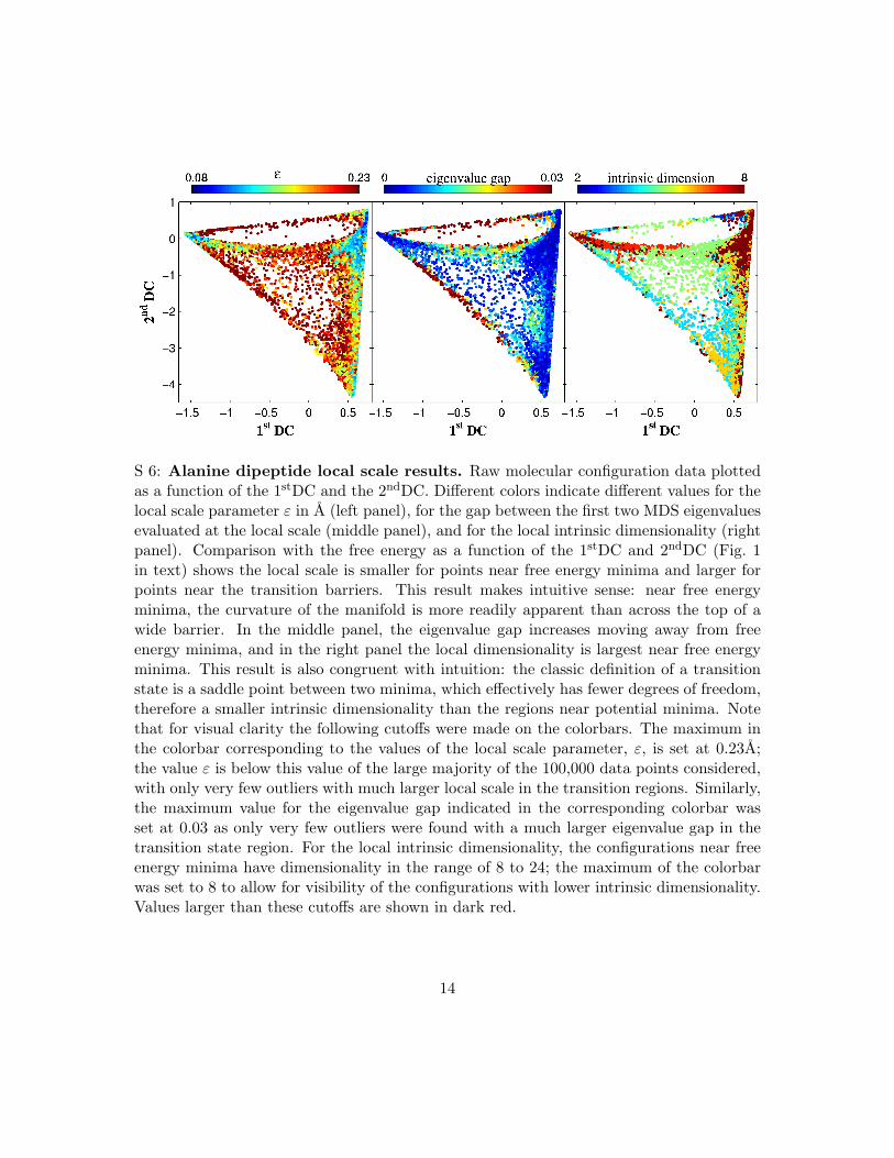
S 6: Alanine dipeptide local scale results. Raw molecular configuration data plottedas a function of the 1stDC and the 2ndDC. Di!erent colors indicate di!erent values for thelocal scale parameter ! in A (left panel), for the gap between the first two MDS eigenvaluesevaluated at the local scale (middle panel), and for the local intrinsic dimensionality (rightpanel). Comparison with the free energy as a function of the 1stDC and 2ndDC (Fig. 1in text) shows the local scale is smaller for points near free energy minima and larger forpoints near the transition barriers. This result makes intuitive sense: near free energyminima, the curvature of the manifold is more readily apparent than across the top of awide barrier. In the middle panel, the eigenvalue gap increases moving away from freeenergy minima, and in the right panel the local dimensionality is largest near free energyminima. This result is also congruent with intuition: the classic definition of a transitionstate is a saddle point between two minima, which e!ectively has fewer degrees of freedom,therefore a smaller intrinsic dimensionality than the regions near potential minima. Notethat for visual clarity the following cuto!s were made on the colorbars. The maximum inthe colorbar corresponding to the values of the local scale parameter, !, is set at 0.23A;the value ! is below this value of the large majority of the 100,000 data points considered,with only very few outliers with much larger local scale in the transition regions. Similarly,the maximum value for the eigenvalue gap indicated in the corresponding colorbar wasset at 0.03 as only very few outliers were found with a much larger eigenvalue gap in thetransition state region. For the local intrinsic dimensionality, the configurations near freeenergy minima have dimensionality in the range of 8 to 24; the maximum of the colorbarwas set to 8 to allow for visibility of the configurations with lower intrinsic dimensionality.Values larger than these cuto!s are shown in dark red.

14

S 7: SH3 local scale results. Raw molecular configuration data plotted as a function ofthe 1stDC and the 2ndDC. The di!erent color indicate di!erent values for the local scale !in nm (left panel), gap between the first two MDS eigenvalues (middle), and local intrinsicdimensionality (right). Comparison with the free energy as a function of the 1stDC and2ndDC (Fig. 3 in text), shows the local scale is smaller for points near the potential energyminimum corresponding to the folded state, and becomes larger for configurations in theentropic free energy minimum corresponding to the unfolded state. A similar trend is ob-served for the eigenvalue gap. This shows that while the curvature of the manifold is readilyapparent in the folded minimum at small length scales, in the unfolded entropic minimum,the manifold is flat for comparatively larger length scales. As for alanine dipeptide, thelocal intrinsic dimensionality is largest for configuration in the free energy minima, bothin the folded and unfolded states, and smallest along the barrier between these two states.Note that for visual clarity the following cuto!s were selected in the colorbars. For theeigenvalue gap, the maximum value was set at 0.08; there are very few outliers with a muchlarger eigenvalue gap near the transition region. Values larger than these cuto!s are shownin dark red.

15

S 8: Analysis of constant-! di!usion map calculation. Left: Alanine dipeptide;

Right: SH3. The top panel of both sides shows the exponential of the negative of theFokker-Planck eigenvalues as a function of ! (units of ! are A for alanine and nm forSH3). As with the locally scaled (local-!) di!usion map calculation, the largest of these,exp(!"0) = 1, corresponds to the Boltzmann distribution, and the presence of a spectralgap between the remaining exp(!"i) indicates a separation of timescales. The bottompanel of both sides shows in blue symbols the reaction rates along the constant-! 1stDC,and in black symbols the correlation of the constant-! 1stDC with the local-! 1stDC forconfigurations in the transition region. For alanine, constant-! isomerization rate for the#R ,#P " C5, P! transition is shown with blue squares. The corresponding rate (anderror) along the local-! 1stDC (from Table 1 in the main text) is indicated by the redshaded region, and the rate obtained directly from simulation is shown as the dot-dashedblack line (the error range is too small to see on this scale). The constant-! isomerizationrate for the C5, P! " #R ,#P transition is shown in blue triangles, the corresponding local-! rate is indicated by gold shaded region, and the simulation rate as the black dashed line.For SH3, both the folding and unfolding rates are similar, and therefore only the unfoldingrate is shown (blue squares). The red shaded region is the rate along the local-! 1stDC;the grey shaded region is the rate obtained directly from simulation (the values reportedin Table 2 of the main text).

16

S 9: Alanine Dipeptide. Left: ! = 0.3 A, Right: ! = 1.0 A. Free energy of alaninedipeptide as a function of 1stDC and 2ndDC obtained from constant-! di!usion map calcu-lations (top panel), and free energy along 1stDC for the same values of ! (bottom panel).For the smaller ! value, the free energy looks very similar to that obtained with the locallyscaled (local-!) di!usion map; however the reaction rate is too low (shown in Figure S8)because the small-! di!usion map calculation places too many molecular configurations inthe free energy wells and too few along the transition region. For the large-! calculation,the di!usion map coordinates are rotated; the free energy along 1stDC has componentsfrom not only "R ,"P ! C5, P!, as in the local-! di!usion map calculation, but also the"R ! "P , and P! ! C5 isomerizations. Therefore there is no clear separation of thedi!erent time scales along the various di!usion map coordinates, as can be expected fromthe lack of a spectral gap for ! = 1.0 in the upper left panel of Figure S8.

17

S 10: SH3. Left: ! = 0.4 nm. Right: ! = 1.6 nm. Free energy of SH3 as afunction of the first two di!usion map coordinates obtained from constant-! di!usion mapcalculations (top panel), and free energy along 1stDC for the same values of ! (bottompanel). For both of these (and for all values of ! considered in Figure S8) the entropyminimum corresponding to the unfolded state almost vanishes. In addition, the crescentshape apparent in the local-! calculation (upper panel of Figure 3 in the main text) is alsodiminished here. Therefore the physical interpretation of 2ndDC in the local-! di!usionmap calculation is not evident here.

18

0.043

0.047

0.051

!R

,!P "

C5,P

##

0.5 0.6 0.7 0.8

0.006 0.009 0.012

0.021

0.023

0.025

C5,P

## "

!R

,!P

cell size2

0.036

0.042

0.048

!R

,!P "

C5,P

##

0.5 0.6

100 150 200

0.018

0.02

0.022

C5,P

## "

!R

,!P

cell size2 (degrees

2)

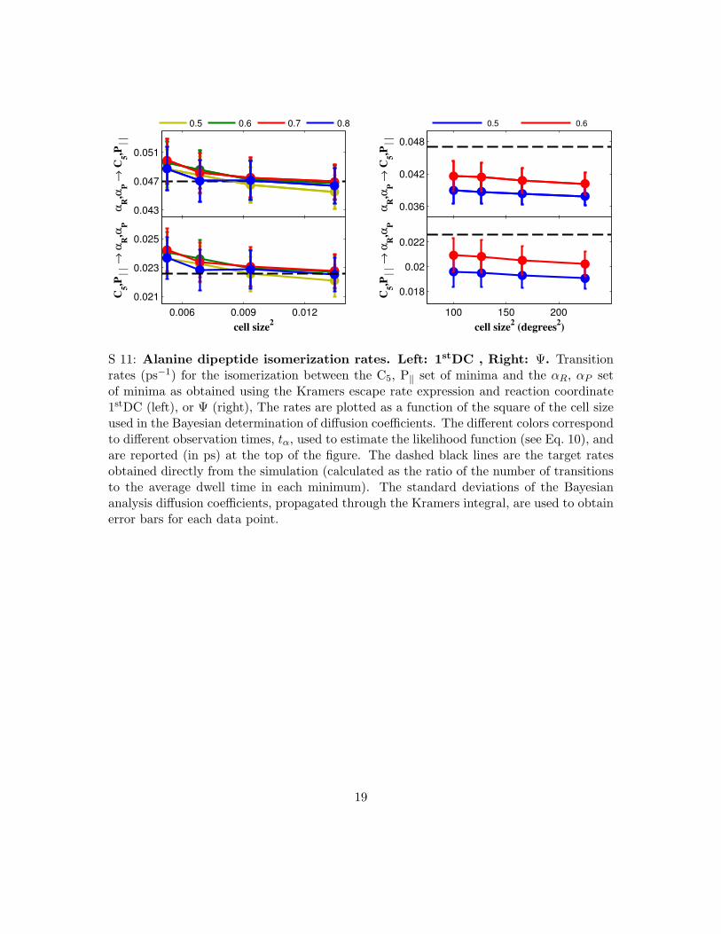
S 11: Alanine dipeptide isomerization rates. Left: 1stDC , Right: !. Transitionrates (ps!1) for the isomerization between the C5, P" set of minima and the !R, !P setof minima as obtained using the Kramers escape rate expression and reaction coordinate1stDC (left), or ! (right), The rates are plotted as a function of the square of the cell sizeused in the Bayesian determination of di"usion coe#cients. The di"erent colors correspondto di"erent observation times, t!, used to estimate the likelihood function (see Eq. 10), andare reported (in ps) at the top of the figure. The dashed black lines are the target ratesobtained directly from the simulation (calculated as the ratio of the number of transitionsto the average dwell time in each minimum). The standard deviations of the Bayesiananalysis di"usion coe#cients, propagated through the Kramers integral, are used to obtainerror bars for each data point.

19

0.001 0.002 0.0030

0.0001

0.0002

0.0003

0.0004

1/(number of cells)2

fold

ed !

un

fold

ed

1st DC RMSD Q

0.001 0.002 0.0030

0.0001

0.0002

0.0003

0.0004

1/(number of cells)2

un

fold

ed !

fo

lded

t" =60 ps t

" =70 ps

S 12: SH3 transition rates. Left: unfolding, Right: folding. Transition rates (ps!1)for the folding/unfolding transition of SH3 calculated by using the Kramers escape rateexpression along the 1stDC (blue), RMSD with respect to the native structure (green),and Q (red). The di!erent symbols correspond to di!erent observation times, t!, in thedefinition of the Bayesian likelihood function for the di!usion coe"cient determination.The grey shaded regions denote the target rates obtained directly from the simulation (cal-culated as the number of transitions from a given minimum divided by average dwell timein that minimum). The standard deviations of the Bayesian analysis di!usion coe"cients,propagated through the Kramers integral, are used as error bars for each data point.

20