Broadcast in the Rendezvous Model

Philippe Duchon, Nicolas Hanusse, Nasser Saheb, and Akka Zemmari

LaBRI - CNRS - Universite Bordeaux I, 351 Cours de la Liberation, 33405 Talence,France. duchon,hanusse,saheb,zemmari@labri.fr

Abstract. In many large, distributed or mobile networks, broadcastalgorithms are used to update information stored at the nodes. In thispaper, we propose a new model of communication based on rendezvousand analyze a multi-hop distributed algorithm to broadcast a message ina synchronous setting. In the rendezvous model, two neighbors u and vcan communicate if and only if u calls v and v calls u simultaneously.Thus nodes u and v obtain a rendezvous at a meeting point.If m is the number of meeting points, the network can be modeled by agraph of n vertices and m edges. At each round, every vertex chooses arandom neighbor and there is a rendezvous if an edge has been chosenby its two extremities. Rendezvous enable an exchange of informationbetween the two entities. We get sharp lower and upper bounds on thetime complexity in terms of number of rounds to broadcast: we showthat, for any graph, the expected number of rounds is between log n andO(n2). For these two bounds, we prove that there exist some graphs forwhich the expected number of rounds is either O(log n) or Ω(n2). Forspecific topologies, additional bounds are given.

Keywords: Algorithms and data structures, distributed algorithms,graph, broadcast, rendezvous model

1 Introduction

Among the numerous algorithms to broadcast in a synchronized setting, weare witnessing a new tendency of distributed and randomized algorithms, alsocalled gossip-based algorithms: at each instant, any number of broadcasts cantake place simultaneously and we do not give any priority to any particular one.In each round, a node chooses a random neighbor and tries to exchange someinformation. Due to the simplicity of gossip-based algorithm, such an approachprovides reliability and scalability. Contrary to deterministic schemes for whichmessages tend to route in a particular subgraph (for instance a tree), a gossip-based algorithm can be fault-tolerant (or efficient for a dynamic network) sincein a strongly connected network, many paths can be used to transmit a messageto almost every node.

The majority of results deal with the uniform random phone call for whicha node chooses a neighbor uniformly at random. However, such a model doesnot take into account that a given node could be “called” by many nodes si-multaneously implying a potential congestion. A more embarrassing situation is

V. Diekert and M. Habib (Eds.): STACS 2004, LNCS 2996, pp. 559–570, 2004.c© Springer-Verlag Berlin Heidelberg 2004

560 P. Duchon et al.

the one of the radio networks in which a node should be called simultaneouslyby a unique neighbor otherwise the received messages are in collision. In therendezvous model, every node chooses a neighbor and if two neighbors choosethemselves mutually, they can exchange some information. The rendezvous modelis useful if a physical meeting is needed to communicate as in the case of robotsnetwork.

Although the rendezvous model can be used in different settings, we describethe problem of broadcasting a message in a network of robots. A robot is anautonomous entity with a bounded amount of memory having the capacity toperform some tasks and to communicate with other entities by radio when theyare geographically close. Examples of use of such robots are numerous: explo-ration [1,7], navigation (see Survey of [16]), capture of an intruder [3], search forinformation, help to handicapped people or rescue, cleaning of buildings, ... Theliterature contains many efficient algorithms for one robot and multiple robotsare seen as a way to speed up the algorithms. However, in a network of robots[4], the coordination of multiple robots implies complex algorithms. Rendezvousbetween robots can be used in the following setting: consider a set of robotsdistributed on a geometric environment. Even if two robots sharing a regionof navigation (called neighbors) might communicate, they should also be closeenough. It may happen that their own tasks do not give them the opportunityto meet (because their routes are deterministic and never cross) or it may take along time if they navigate at random. A solution consists in deciding on a meet-ing point for each pair of neighbor robots. If two neighbors are close to a givenmeeting point at the same time, they have a rendezvous and can communicate.

Although there exist many algorithms to broadcast messages, we only dealwith algorithms working under a very weak assumption: each node or robot onlyknows its neighbors or its own meeting points. This implies that the underlyingtopology is unknown. Depending on the context, we might also be interestedin anonymous networks in which the labeling of the nodes (or history of thevisited nodes) is not used. By anonymous, we mean that unique identities are notavailable to distinguish nodes (processors) or edges (links). In a robot network,the network can have two (or more) meeting points with the same label if theenvironment contains two pairs of regions that do not overlap. The anonymoussetting can be encountered in dynamic, mobile or heterogeneous networks.

1.1 Related Works

How to broadcast efficiently a message with a very poor knowledge on the topol-ogy of an anonymous network ? Depending on the context, this problem isrelated to the way a “rumor” or an “epidemic” spreads in a graph. In the liter-ature, a node is contaminated if it knows the rumor. The broadcast algorithmhighly depends on the communication model. For instance, in the k-ports model,a node can send a message to at most k neighbors. Thus our rendezvous modelis a 1-port model.

The performance of a broadcast algorithm is measured by the time requiredto contaminate all the nodes, the amount of memory stored at each node orthe total number of messages. In this article, we analyze the time complexity

Broadcast in the Rendezvous Model 561

in a synchronous setting of a rendezvous algorithm (although several broadcastalgorithms including ours can work in an asynchronous setting, the theoreticaltime complexity is usually analyzed in a synchronous model).

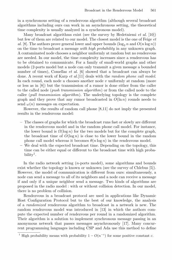
Many broadcast algorithms exist (see the survey by Hedetniemi et al. [10])but few of them are related to our model. The closest model is the one of Feige etal. [8]. The authors prove general lower and upper bounds (log2 n and O(n log n))on the time to broadcast a message with high probability in any unknown graph.A contaminated node chooses a neighbor uniformly at random but no rendezvousare needed. In our model, the time complexity increases since a rendezvous hasto be obtained to communicate. For a family of small-world graphs and othermodels (2-ports model but a node can only transmit a given message a boundednumber of times), Comellas et al. [6] showed that a broadcast can always bedone. A recent work of Karp et al.[11] deals with the random phone call model.In each round, each node u chooses another node v uniformly at random (moreor less as in [8]) but the transmission of a rumor is done either from the callerto the called node (push transmission algorithm) or from the called node to thecaller (pull transmission algorithm). The underlying topology is the completegraph and they prove that any rumor broadcasted in O(lnn) rounds needs tosend ω(n) messages on expectation.

However, the results of random call phone [8,11] do not imply the presentedresults in the rendezvous model:

– The classes of graphs for which the broadcast runs fast or slowly are differentin the rendezvous model and in the random phone call model. For instance,the lower bound is Ω(log n) for the two models but for the complete graph,the broadcast time of O(log n) is close to the lower bound in the randomphone call model whereas it becomes θ(n log n) in the rendezvous model.

– We deal with the expected broadcast time. Depending on the topology, thistime can be either equal or different to the broadcast time with high proba-bility1.

In the radio network setting (n-ports model), some algorithms and boundsexist whether the topology is known or unknown (see the survey of Chlebus [5]).However, the model of communication is different from ours: simultaneously, anode can send a message to all of its neighbors and a node can receive a messageif and only if a unique neighbor send a message. Two kinds of algorithms areproposed in the radio model : with or without collision detection. In our model,there is no problem of collision.

Rendezvous in a broadcast protocol are used in applications like DynamicHost Configuration Protocol but to the best of our knowledge, the analysisof a randomized rendezvous algorithm to broadcast in a network is new. Therandom rendezvous model was introduced in [13] in which the authors com-pute the expected number of rendezvous per round in a randomized algorithm.Their algorithm is a solution to implement synchronous message passing in ananonymous network that passes messages asynchronously [17]. Many concur-rent programming languages including CSP and Ada use this method to define1 High probability means with probability 1 − O(n−c) for some positive constant c.

562 P. Duchon et al.

a communication between pairs of asynchronous processes. Angluin [2] provedthat there is no deterministic algorithm for this problem (see the paper of Lynch[12] containing many problems having no deterministic solutions in distributedcomputing) . In [14], the rendezvous are used to elect randomly a leader in ananonymous graph.

1.2 The Model

Let G = (V, E) be a connected and undirected graph of n vertices and m edges.For convenience and with respect to the problem of spreading an epidemic, avertex is contaminated if it has received the message sent by an initial vertex v0.

The model can be implemented in a fully distributed way. The complexityanalysis, however based on the concept of rounds, is commonly used in similarstudies [8,13,14]. In our article, a round is the following sequence:

– for each v ∈ V , choose uniformly at random an incident edge.– if an edge (vi, vj) has been chosen by vi and vj , there is a rendezvous.– if there is a rendezvous and if only vi is contaminated, then vj becomes

contaminated.

TG is the broadcast time or contamination time, that is the number of roundsuntil all vertices of graph G are contaminated. TG is an integer-valued randomvariable; in this paper, we concentrate the study on its expectation E(TG).

Some remarks can be made on our model. As explained in the introduction,the rendezvous process (the first two steps of the round) keeps repeating foreverand should be seen as a way of maintaining connectivity. Several broadcasts cantake place simultaneously and we do not give any priority to any one of them,even if we study a broadcast starting from a given vertex v0.

We concentrate our effort on E(TG) and we do not require that the algorithmfinds out when the rumor sent by v0 has reached all the nodes. However somehints can be given: we can stop the broadcast algorithm (do not run the thirdstep of the round) using a local control mechanism in each node of the network:if identities of the nodes are available (non anonymous networks), each nodekeeps into its memory a list of contaminated neighbors for each rumor and whenthis list contains all the neighbors, the process may stop trying to contaminatethem (with the same rumor). If the network is anonymous and the number ofnodes n is known, then it is possible to prove that in O(n2 log n) rounds withhigh probability, all the neighbors of a contaminated node know the rumor.

In our algorithm, nodes of large degree and a large diameter increase thecontamination time. Taking two adjacent nodes vi and vj of degrees di and dj

respectively, the expected number of rounds to contaminate vj from vi is didj .For instance, take two stars of n/2 leaves. Join each center by an edge. In therendezvous model, the expected broadcast time is Θ(n2) whereas in [8]’s model,it will be Θ(n log n) on expectation and with high probability. Starting from thisexample, E(TG) can easily be upper bounded by O(n3) but we find a tighterupper bound.

Broadcast in the Rendezvous Model 563

1.3 Our Results

The main result of the paper is to prove in Section 2 that for any graph G,log2 n ≤ E(TG) ≤ O(n2). More precisely, for any graph G of maximal degree ∆,E(TG) = O(∆n).

In Section 3, we show that there are some graphs for which the expectedbroadcast time asymptotically matches either the lower bound or the upperbound up to a constant factor. For instance, for the complete balanced binarytree, E(TG) = O(log2 n) whereas E(TG) = Ω(n2) for the double star graph (twoidentical stars joined by one edge). For graphs of bounded degree ∆ and diameterD, we also prove in Section 3 that E(TG) = O(D∆2 ln∆). This upper bound istight since for ∆-ary complete trees of diameter D, E(TG) = Ω(D∆2 ln∆). Thecomplete graph was proved [13] to have the least expected number of rendezvousper round; nevertheless, its expected broadcast time is Θ(n lnn). Due to spacelimitations, proofs of lemmas and corollaries are not given.

2 Arbitrary Graphs

The first section presents some terminology and basic lemmas that are useful forthe main results.

2.1 Generalities on the Broadcast Process

The rendezvous process induces a broadcast process, that is, for each nonnegativeinteger t, we get a (random) set of vertices, Vt, which is the set of verticesthat have been reached by the broadcast after t rounds of rendezvous. Thesequence (Vt)t∈N is a homogeneous, increasing Markov process with state spaceU : ∅ U ⊂ V . Any state U contains the initial vertex v0 and the subgraphinduced by U is connected. State V as its sole absorbing state; thus, for eachgraph G, this process reaches state V (that is, the broadcast is complete) infinite expected time.

The transition probabilities for this Markov chain (Vk) depend on the ren-dezvous model. Specifically, if U and U ′ are two nonempty subsets of V , thetransition probability pU,U ′ is 0 if U U ′, and, if U ⊆ U ′, pU,U ′ is the proba-bility that, on a given round of rendezvous, U ′ − U is the set of vertices not inU that have a rendezvous with a vertex in U . Thus, the loop probability pU,U isthe probability that each vertex in U either has no rendezvous, or has one withanother vertex in U .

In the sequel, what we call the broadcast sequence is the sequence of distinctstates visited by the broadcast process between the initial state v0 and the finalabsorbing state V . A possible broadcast sequence is any sequence of states thathas a positive probability of being the broadcast sequence; this is any sequenceX = (X1, . . . , Xm) such that X1 = V0 = v0, Xm = V , and pXk,Xk+1 > 0 forall k.

By du we denote the degree of vertex u. For a bounded degree graph, ∆ isthe maximal degree of the graph. By D we denote the diameter of the graph.

564 P. Duchon et al.

If Xk = Vt is the set of the k contaminated vertices at time t then Yk is theset of remaining vertices. We define the cut Ck as the set of edges that have oneendpoint in Xk and the other in Yk.

For any edge a = (u, v) ∈ E, P(a) = (dudv)−1 (resp. P(a)) is the probabilitythat edge a will obtain (resp. not obtain) a rendezvous at a given round. Theproduct (dudv)−1 is also called the weight of the edge a.

We also define two values for any set of edges C ⊂ E : P(EC) (resp. P(EC))where EC is the event of obtaining a rendezvous in a round for at least one edge(resp. no edge) in C; and π(C) =

∑a∈C P(a). While π(C) has no direct proba-

bilistic interpretation, it is much easier to deal with in computations. Obviously,P(EC) ≤ π(C) holds for any C. Lemma 2 provides us with a lower bound forP(EC) of the form Ω(π(C)) provided π(C) is not too large.

With these notations, for any set of vertices U , pU,U = 1 − P(ECU), where

CU is the set of edges that have exactly one endpoint in U (the cut defined bythe partition (U, V − U)).

Lemma 1. Let a ∈ E and for any C ⊂ E, P(a | EC) ≥ P(a).

Lemma 2. For any C ⊂ E, P(EC) ≥ λ min(1, π(C)) with λ = 1 − e−1 wheree = exp(1).

Corollary 1.

1P(EC)

≤ e

e − 1max

(

1,1

π(C)

)

≤ e

e − 1

(

1 +1

π(C)

)

. (1)

Lemma 3. For any graph G, any integer k and any p ∈ (0, 1), if P(TG > k) ≤ pthen E(TG) ≤ k/(1 − p).

Since the number of contaminated vertices can be at most doubled at eachround, we have the following trivial lower bound

Theorem 1. For any graph G, TG ≥ log2 n with probability 1.

2.2 The General Upper Bound

We will prove the following :

Theorem 2. For any connected graph G with n vertices and maximum degree∆, the broadcast time TG satisfies

E(TG) ≤ e

e − 1(n − 1)(6∆ + 1). (2)

Broadcast in the Rendezvous Model 565

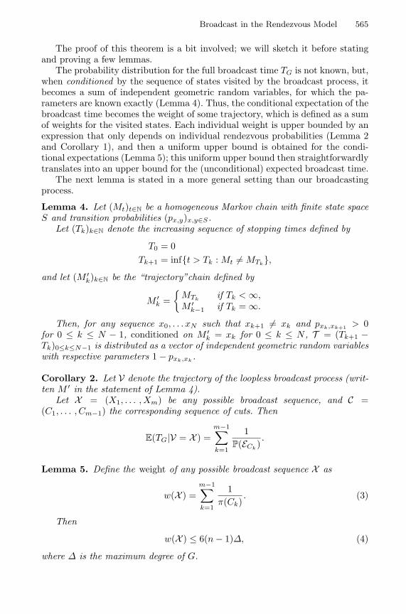
The proof of this theorem is a bit involved; we will sketch it before statingand proving a few lemmas.

The probability distribution for the full broadcast time TG is not known, but,when conditioned by the sequence of states visited by the broadcast process, itbecomes a sum of independent geometric random variables, for which the pa-rameters are known exactly (Lemma 4). Thus, the conditional expectation of thebroadcast time becomes the weight of some trajectory, which is defined as a sumof weights for the visited states. Each individual weight is upper bounded by anexpression that only depends on individual rendezvous probabilities (Lemma 2and Corollary 1), and then a uniform upper bound is obtained for the condi-tional expectations (Lemma 5); this uniform upper bound then straightforwardlytranslates into an upper bound for the (unconditional) expected broadcast time.

The next lemma is stated in a more general setting than our broadcastingprocess.

Lemma 4. Let (Mt)t∈N be a homogeneous Markov chain with finite state spaceS and transition probabilities (px,y)x,y∈S.

Let (Tk)k∈N denote the increasing sequence of stopping times defined by

T0 = 0Tk+1 = inft > Tk : Mt = MTk

,

and let (M ′k)k∈N be the “trajectory”chain defined by

M ′k =

MTk

if Tk < ∞,M ′

k−1 if Tk = ∞.

Then, for any sequence x0, . . . xN such that xk+1 = xk and pxk,xk+1 > 0for 0 ≤ k ≤ N − 1, conditioned on M ′

k = xk for 0 ≤ k ≤ N , T = (Tk+1 −Tk)0≤k≤N−1 is distributed as a vector of independent geometric random variableswith respective parameters 1 − pxk,xk

.

Corollary 2. Let V denote the trajectory of the loopless broadcast process (writ-ten M ′ in the statement of Lemma 4).

Let X = (X1, . . . , Xm) be any possible broadcast sequence, and C =(C1, . . . , Cm−1) the corresponding sequence of cuts. Then

E(TG|V = X ) =m−1∑

k=1

1P(ECk

).

Lemma 5. Define the weight of any possible broadcast sequence X as

w(X ) =m−1∑

k=1

1π(Ck)

. (3)

Then

w(X ) ≤ 6(n − 1)∆, (4)

where ∆ is the maximum degree of G.

566 P. Duchon et al.

Proof. We begin by noting that, since we are looking for a uniform upper boundon the weight, we can assume that m = n, which is equivalent to |Xk| = k for allk. If such is not the case in a sequence X , then we can obtain another possiblesequence X ′ with a higher weight by inserting an additional set X ′ between anytwo consecutive sets Xk and Xk+1 such that |Xk+1−Xk| ≥ 2 (with the conditionthat pXk,X′ and pX′,Xk+1 are both positive; such an X ′ always exists, becauseeach edge of every graph has positive probability of being the only rendezvousedge in a given round). This will just add a positive term to the weight of thesequence; thus, the sequence with the maximum weight satisfies m = n.

To prove that∑n−1

k=1 1/π(Ck) ≤ 6(n−1)∆, we prove that the integer interval[1, n − 1] can be partitioned into a sequence of smaller intervals, such that, oneach interval, the average value of 1/π(Ck) is at most 6∆.

Assume that integers 1 to k − 1 have been thus partitioned, and let us con-sider Ck. If π(Ck) ≥ 1/(4∆) (that is, 1/π(Ck) ≤ 4∆ < 6∆), we put k into aninterval by itself and move on to k + 1. We now assume π(Ck) < 1/(4∆), andset 1/π(Ck) = α∆ with α > 4.

Let v be the next vertex to be reached by the broadcast after Xk, that is,v = Xk+1 − Xk. This vertex must have at least one neighbor u in Xk.

Let d ≥ 1 denote the number of neighbors of v that are in Xk. Each edgeincident to v has weight at least 1/(dv∆), and d of them are in Ck, so that wehave d/(dv∆) ≤ π(Ck) = 1/(α∆), or equivalently,

d ≤ dv/α. (5)

Thus, v ∈ Xk+1 has dv − d neighbors in Yk+1 = V − Xk+1. Since at mostone of them is added to X at each step of the sequence, this means that, for0 ≤ j ≤ dv − d, Yk+1+j contains at least dv − d − j neighbors of v. In otherwords, Ck+1+j contains at least dv − d − j edges that are incident to v, each ofwhich has weight at least 1/(dv∆). Consequently,

1π(Ck+1+j)

≤ dv∆

dv − d − j(6)

holds for 0 ≤ j ≤ dv − d.The right-hand side of (6) increases with j, and for j = dv/4 (recall eq. (5)

and α > 4), it is

dv∆

dv − d − dv/4 ≤ dv∆

dv − 2dv/4

≤ dv∆

dv/2≤ 2∆.

Summing (6) over 0 ≤ j ≤ dv/4, we obtain

dv/4∑

j=0

1π(Ck + 1 + j)

≤ 2∆

(

1 +dv

4

)

. (7)

Broadcast in the Rendezvous Model 567

Since dv ≥ α, we also have 1/π(Ck) ≤ dv∆. Adding this to 7, we now get

1π(Ck)

+∑

0≤j≤dv/4

1π(Ck + 1 + j)

≤ ∆

(

α + 2 +dv

2

)

≤ ∆

(

2 +3dv

2

)

.

There are 2 + dv/4 ≥ 1 + dv

4 terms in the left-hand side of this inequality,so that the average value of 1/π(Ci), when i ranges over [k, k + 1 + dv/4], isat most

∆2 + 3dv

2

1 + dv

4

≤ 6∆. (8)

This concludes the recursion, and the proof.

Proof (Theorem 2).Let X be any possible broadcast sequence as in Lemma 5. Applying Corol-

lary 1 to C = Ck and summing over k, we get

∑

k

1P(ECk

)≤ e

e − 1

(

n − 1 +∑

k

1π(Ck)

)

. (9)

By Lemma 5, the right-hand side of (9) is at most

e

e − 1(n − 1 + 6∆(n − 1)) =

e(n − 1)(6∆ + 1)e − 1

. (10)

By Lemma 4, the left-hand side of (9) is the conditional expectation of TG.The upper bound remains valid upon taking a convex linear combination, sothat we get, as claimed,

E(TG) ≤ e(n − 1)(6∆ + 1)e − 1

. (11)

Note: It should be clear that the constants are not best possible, even with ourmethod of proof. They are, however, quite sufficient for our purpose, which is toobtain a uniform bound on the expected broadcast time.

3 Specific Graphs

Theorems 1 and 2 provide lower and upper bounds on the expected contamina-tion time for any graph. In this section, we prove that there exists some graphsfor which the bounds can be attained.

The well-known coupon-collector problem (that is the number of trials re-quired to obtain n different coupons if each round one is chosen randomly andindependently. See [15] for instance) implies the next lemma:

Lemma 6. For a star S of n leaves, E(TS) = n lnn + O(n).

568 P. Duchon et al.

3.1 The l-Star Graphs

An l-star graph Sl is a graph built with a chain of l + 2 vertices. Then foreach vertex different to the extremities, ∆ − 2 leaves are added. Let Sl be al-star graphs with n = l(∆ − 1) + 2 vertices. According to Theorem 2, E(TSl

) =O(∆n) = O(n2

l ). On the other hand, the expected number of rounds to geta rendezvous between centers of two adjacent stars is ∆2 and, therefore, theexpected number of rounds for contaminating all the centers is Ω(l∆2) = Ω(n∆).As a corollary to this result we have

Proposition 1. There exists an infinite family of graphs F of n vertices andmaximal degree ∆ such that, for any G ∈ F , E(TG) = Ω(∆n).

It follows that the general upper bound O(n2) given by Theorem 2 is tight forthe any l-star graph with l ≥ 2 constant.

3.2 Matching the Lower Bound

To prove that the Ω(log n) bound is tight, we prove an upper bound that onlyinvolves the maximum degree ∆ and the diameter D.

Theorem 3. Let G be any graph with maximum degree ∆ ≥ 3 and diameterD. Then the expected broadcast time in G, starting from any vertex, is at most4∆2 (ln 2 + D + D ln∆).

Our proof of this theorem will make use of the following lemma.

Lemma 7. Fix a constant p > 0, and let Sk denote the sum of k independentgeometric random variables with parameter p.

Then, for any t ≥ k/p, we have

P(Sk > t) ≤ exp

(

− tp

2

(

1 − k

tp

)2)

.

Proof (Theorem 3). We prove that the probability for the broadcast time toexceed half of the claimed bound is at most 1/2 and then use Lemma 3.

Let u be the initial vertex for the broadcast. For each other vertex v, picka path γuv from u to v with length at most D. Since all degrees are at most∆, each edge in γuv has a rendezvous probability at least 1/∆2. Hence, thebroadcast time from u to v along the path γuv (that is, the time until the firstedge has a rendezvous, then the second edge, and so on) is distributed as thesum of independent geometric random variables with parameters equal to therendezvous probabilities, and is thus stochastically dominated by the sum of Dindependent geometric random variables with parameter 1/∆2.

Let Tuv denote the time until broadcast reaches v when the initial vertex isu; Lemma 7 and the above discussion imply, for any t,

P(Tuv > t) ≤ e− t

2∆2

(1− D∆2

t

)2

. (12)

Broadcast in the Rendezvous Model 569

Let 1 + n denote the number of vertices in G. Moore’s bound ensures thatn ≤ ∆D.

It is routine to check that, if t > 2∆2(ln 2+D+D ln∆), then t(1−D∆2/t)2 >2∆2(ln 2 + D ln∆) ≥ 2∆2 ln(2n). Thus, for each of the n vertices v = u, we get

P(Tuv > t) ≤ e− ln(2n) =12n

, (13)

so that, summing over v, we get

P(Tu > t) ≤ 12. (14)

Corollary 3. There exists an infinite family of graphs F such that, for anyG ∈ F , E(TG) = O(log |G|).

3.3 The Complete Graph

It is seems also interesting to point out that the complete graph Kn has theminimal (see [13]) expected rendezvous number in a round:

E(NKn) =

(n2

)

(n − 1)2,

which is asymptotically 12 . We prove in this section that its expected broadcast

time is however O(n lnn), which is significantly shorter than that of the l-stargraph with l constant which is Ω(n2).

Lemma 8. E(TKn) ≤ 2λ−1n lnn + O(n).

Moreover, we have:

Lemma 9. With probability 1 − n−1/2, E(TKn) ≥ 1

2n lnn.

Lemmas 9 and 8 imply:

Proposition 2. E(TKn) = Θ(n lnn).

3.4 Graphs of Bounded Degree and Bounded Diameter

Lemma 10. Let G be a ∆-regular balanced complete rooted tree of depth 2. Theexpected time for the root to contaminate its children is Θ(∆2 ln∆).

Theorem 4. Let G be a ∆-regular balanced complete rooted tree of depth D/2with D even. E(TG) = Ω(D∆2 ln∆).

Proof. Suppose the broadcast starts from the root v0. Let us construct a pathv0, v1, v2, . . . , vD/2 such that vi is the last contaminated child of vi−1. Tvi de-notes the number of rounds to contaminate vj by its parent vi−1 once vi−1 iscontaminated. Since TG ≥

∑D/2i=1 Tvi and from Lemma 10, for every 1 ≤ i ≤ D/2,

E(Tvi) = Θ(∆2 ln∆), we have E(TG) ≥∑D/2

i=1 E(Tvi) = Ω(D∆2 ln∆).

Theorem 4 proves that there exists a graph for which the upper bound ofTheorem 3 is tight.

570 P. Duchon et al.

References

1. S. Albers and M. Henzinger. Exploring unknown environments. SIAM Journal onComputing, 29(4):1164–1188, 2000.

2. D. Angluin. Local and global properties in networks of processors. In Proceedingsof the 12th Symposium on theory of computing, pages 82–93, 1980.

3. L. Barriere, P. Flocchini, P. Fraigniaud, and N. Santoro. Capture of an intruderby mobile agents. In In 14th ACM Symposium on Parallel Algorithms and Archi-tectures (SPAA), pages 200–209, 2002.

4. Michael A. Bender and Donna K. Slonim. The power of team exploration: tworobots can learn unlabeled directed graphs. In Proceedings of the 35rd AnnualSymposium on Foundations of Computer Science, pages 75–85. IEEE ComputerSociety Press, Los Alamitos, CA, 1994.

5. B. Chlebus. Handbook on Randomized Computing, chapter Randomized commu-nication in radio networks. Kluwer Academic, to appear.http://citeseer.nj.nec.com/489613.html.

6. Francesc Comellas, Javier Ozon, and Joseph G. Peters. Deterministic small-worldcommunication networks. Information Processing Letters, 76(1–2):83–90, 2000.

7. Xiaotie Deng, Tiko Kameda, and Christos H. Papadimitriou. How to learn anunknown environment i: The rectilinear case. Journal of the ACM, 45(2):215–245,1998.

8. Uriel Feige, David Peleg, Prabhakar Raghavan, and Eli Upfal. Randomized broad-cast in networks. Random Structures and Algorithms, 1, 1990.

9. M. Habib, C. McDiarmid, J. Ramirez-Alfonsin, and B. Reed, editors. ProbabilisticMethods for Algorithmic Discrete Mathematics. Springer, 1998.

10. S.M. Hedetniemi, S.T. Hedetniemi, and A.L. Liestman. A survey of gossiping andbroadcasting in communication networks. Networks, 18:319–349, 1988.

11. Richard M. Karp, Christian Schindelhauer, Scott Shenker, and Berthold Vocking.Randomized rumor spreading. In IEEE Symposium on Foundations of ComputerScience, pages 565–574, 2000.

12. N. Lynch. A hundred impossibility proofs for distributed computing. In Proceedingsof the 8th ACM Symposium on Principles of Distributed Computing (PODC), pages1–28, New York, NY, 1989. ACM Press.

13. Yves Metivier, Nasser Saheb, and Akka Zemmari. Randomized rendezvous. Trendsin mathematics, pages 183–194, 2000.

14. Yves Metivier, Nasser Saheb, and Akka Zemmari. Randomized local elections.Information processing letters, 82:313–320, 2002.

15. R. Motwani and P. Raghavan. Randomized Algorithms. Cambridge Univ. Press,1995.

16. N. Rao, S. Kareti, W. Shi, and S. Iyenagar. Robot navigation in unknown terrains:Introductory survey of non-heuristic algorithms, 1993.http://citeseer.nj.nec.com/rao93robot.html.

17. G. Tel. Introduction to distributed algorithms. Cambridge University Press, 2000.