Semi-Supervised Learning with Sparse Autoencoders in ...
52
IN DEGREE PROJECT COMPUTER SCIENCE AND ENGINEERING, SECOND CYCLE, 30 CREDITS , STOCKHOLM SWEDEN 2016 Semi-Supervised Learning with Sparse Autoencoders in Automatic Speech Recognition AKASH KUMAR DHAKA KTH ROYAL INSTITUTE OF TECHNOLOGY SCHOOL OF COMPUTER SCIENCE AND COMMUNICATION
-
Upload
khangminh22 -
Category
Documents
-
view
3 -
download
0
Transcript of Semi-Supervised Learning with Sparse Autoencoders in ...
IN DEGREE PROJECT COMPUTER SCIENCE AND ENGINEERING,SECOND CYCLE, 30 CREDITS
, STOCKHOLM SWEDEN 2016
Semi-Supervised Learning with Sparse Autoencoders in Automatic Speech Recognition
AKASH KUMAR DHAKA
KTH ROYAL INSTITUTE OF TECHNOLOGYSCHOOL OF COMPUTER SCIENCE AND COMMUNICATION

Semi-Supervised Learning with SparseAutoencoders in Automatic SpeechRecognition
AKASH KUMAR DHAKA
Master in Machine LearningDate: November 2016Supervisor: Giampiero SalviExaminer: Danica KragicSwedish title: Semi-övervakad inlärning med glesa autoencoders iautomatisk taligenkänningSchool of Computer Science and Communication
Abstract
This work is aimed at exploring semi-supervised learning techniques to improve theperformance of Automatic Speech Recognition systems. Semi-supervised learning takesadvantage of unlabeled data in order to improve the quality of the representations ex-tracted from the data. The proposed model is a neural network where the weights areupdated by minimizing the weighted sum of a supervised and an unsupervised costfunction, simultaneously. These costs are evaluated on the labeled and unlabeled por-tions of the data set, respectively. The combined cost is optimized through mini-batchstochastic gradient descent via standard backpropagation.
The model was tested on a phone classification task on the TIMIT American Englishdata set and on a written digit classification task on the MNIST data set. Our resultsshow that the model outperforms a network trained with standard backpropagation onthe labelled material alone. The results are also in line with state-of-the-art graph-basedsemi-supervised training methods.
Sammanfattning
Detta arbete syftar till att utforska halvövervakade inlärningstekniker (eng: semi-supervisedlearning techniques) för att förbättra prestandan hos automatiska taligenkänningssystem.Halvövervakad maskininlärning använder sig av data ej märkt med klasstillhörighets-information för att förbättra kvaliteten hos den från datan extraherade representationen.Modellen som beskrivs i arbetet är ett neuralt nätverk där vikterna uppdateras genom attsamtidigt minimera den viktade summan av en övervakad och en oövervakad kostnads-funktion. Dessa kostnadsfunktioner evalueras på den märkta respektive den omärkta da-tamängden. De kombinerade kostnadsfunktionerna optimeras genom gradient descentmed hjälp av traditionell backpropagation.
Modellen har evaluerats genom en fonklassificeringsuppgift på datamängden TIMITAmerican English, samt en sifferklassificeringsuppgift på datamängden MNIST. Resul-taten visar att modellen presterar bättre än ett nätverk tränat med backpropagation påendast märkt data. Resultaten är även konkurrenskraftiga med rådande state of the art,grafbaserade halvövervakade inlärningsmetoder.

Contents
1 Introduction 11.1 The Speech Recognition Problem . . . . . . . . . . . . . . . . . . . . . . . . . . 11.2 Motivation For the Thesis . . . . . . . . . . . . . . . . . . . . . . . . . . . . . . 21.3 Research Questions . . . . . . . . . . . . . . . . . . . . . . . . . . . . . . . . . . 31.4 Assumptions . . . . . . . . . . . . . . . . . . . . . . . . . . . . . . . . . . . . . . 31.5 Report Structure . . . . . . . . . . . . . . . . . . . . . . . . . . . . . . . . . . . . 3
2 Relevant Theory 42.1 Automatic Speech Recognition and Phone Classification . . . . . . . . . . . . 42.2 Feature Extraction . . . . . . . . . . . . . . . . . . . . . . . . . . . . . . . . . . . 62.3 Acoustic Modelling . . . . . . . . . . . . . . . . . . . . . . . . . . . . . . . . . . 72.4 MLPs and Deep Neural Networks . . . . . . . . . . . . . . . . . . . . . . . . . 92.5 Autoencoders . . . . . . . . . . . . . . . . . . . . . . . . . . . . . . . . . . . . . 11
2.5.1 Manifold Learning with Autoencoders . . . . . . . . . . . . . . . . . . 112.5.2 Sparse Autoencoders . . . . . . . . . . . . . . . . . . . . . . . . . . . . . 122.5.3 Performance of Sparse Autoencoders . . . . . . . . . . . . . . . . . . . 122.5.4 Applications of Autoencoders . . . . . . . . . . . . . . . . . . . . . . . 13
2.6 Semi-Supervised Learning . . . . . . . . . . . . . . . . . . . . . . . . . . . . . . 132.7 Assumptions . . . . . . . . . . . . . . . . . . . . . . . . . . . . . . . . . . . . . . 14
3 Related Work 153.1 Deep Neural Networks in ASR . . . . . . . . . . . . . . . . . . . . . . . . . . . 15
3.1.1 Deep Belief Networks . . . . . . . . . . . . . . . . . . . . . . . . . . . . 153.1.2 Recurrent Neural Networks . . . . . . . . . . . . . . . . . . . . . . . . 15
3.2 Examples of Semi-Supervised Learning Methods . . . . . . . . . . . . . . . . 163.2.1 Heuristic based SSL/Self-Training . . . . . . . . . . . . . . . . . . . . . 163.2.2 Transductive SVMs . . . . . . . . . . . . . . . . . . . . . . . . . . . . . . 163.2.3 Entropy Based Semi Supervised Learning . . . . . . . . . . . . . . . . 173.2.4 Graph based SSL . . . . . . . . . . . . . . . . . . . . . . . . . . . . . . . 173.2.5 Semi-Supervised Learning with generative models . . . . . . . . . . . 18
3.3 Autoencoder Based Semi-Supervised Learning . . . . . . . . . . . . . . . . . . 19
4 Method 204.1 The Model . . . . . . . . . . . . . . . . . . . . . . . . . . . . . . . . . . . . . . . 204.2 Evaluation . . . . . . . . . . . . . . . . . . . . . . . . . . . . . . . . . . . . . . . 224.3 Monitoring and Debugging . . . . . . . . . . . . . . . . . . . . . . . . . . . . . 23
4.3.1 Design Choices/Tuning Hyperparameters . . . . . . . . . . . . . . . . 23
4.3.2 Learning Rate . . . . . . . . . . . . . . . . . . . . . . . . . . . . . . . . . 244.3.3 Batch Size . . . . . . . . . . . . . . . . . . . . . . . . . . . . . . . . . . . 254.3.4 Weight Initialization . . . . . . . . . . . . . . . . . . . . . . . . . . . . . 254.3.5 Number of Hidden Units . . . . . . . . . . . . . . . . . . . . . . . . . . 254.3.6 Momentum . . . . . . . . . . . . . . . . . . . . . . . . . . . . . . . . . . 264.3.7 Activation Function . . . . . . . . . . . . . . . . . . . . . . . . . . . . . 264.3.8 Training Epochs . . . . . . . . . . . . . . . . . . . . . . . . . . . . . . . 264.3.9 Additive Noise . . . . . . . . . . . . . . . . . . . . . . . . . . . . . . . . 264.3.10 Alpha . . . . . . . . . . . . . . . . . . . . . . . . . . . . . . . . . . . . . 264.3.11 Gradient Checking . . . . . . . . . . . . . . . . . . . . . . . . . . . . . . 27
5 Experiment Setup and Results 285.1 Data . . . . . . . . . . . . . . . . . . . . . . . . . . . . . . . . . . . . . . . . . . . 28
5.1.1 MNIST . . . . . . . . . . . . . . . . . . . . . . . . . . . . . . . . . . . . . 285.1.2 TIMIT . . . . . . . . . . . . . . . . . . . . . . . . . . . . . . . . . . . . . 28
5.2 Experimental Setup . . . . . . . . . . . . . . . . . . . . . . . . . . . . . . . . . . 305.3 Practical Setup . . . . . . . . . . . . . . . . . . . . . . . . . . . . . . . . . . . . . 315.4 Results . . . . . . . . . . . . . . . . . . . . . . . . . . . . . . . . . . . . . . . . . 31
6 Discussion, Conclusion and Future Work 366.1 Hypotheses discussed . . . . . . . . . . . . . . . . . . . . . . . . . . . . . . . . 36
6.1.1 H.1 Do Semi-Supervised Sparse Autoencoders perform better than neu-ral networks on phone classification? . . . . . . . . . . . . . . . . . . . 36
6.1.2 H.2 Does the above result generalize to other domains? . . . . . . . . 366.1.3 H.3: Do Semi-Supervised Sparse Autoencoders perform better than GBL
SSL methods on phoneme classification? . . . . . . . . . . . . . . . . . 366.2 Evaluation Method . . . . . . . . . . . . . . . . . . . . . . . . . . . . . . . . . . 376.3 Effect of α in the model . . . . . . . . . . . . . . . . . . . . . . . . . . . . . . . 376.4 Future Work . . . . . . . . . . . . . . . . . . . . . . . . . . . . . . . . . . . . . . 376.5 Society and Ethics . . . . . . . . . . . . . . . . . . . . . . . . . . . . . . . . . . 38
7 Appendix 39
Bibliography 40
Chapter 1
Introduction
With the invention of computers, the question of whether machines could be made tounderstand human speech emerged. In more recent years, speech technology has startedto change the way we live by becoming an important tool for communication and inter-action with devices. The recent improvements in Spoken Language systems have greatlyimproved Human-Machine Communication. Personal Digital Assistance (PDA) systemsare an example of an intelligent dialogue management system. They have been very pop-ular with the recent launch of products like Apple Siri, Amazon Alexa and Google Allo.Besides human-machine interaction, speech technology has also been applied in assistedhuman-human communication. There could be several barriers even when humans com-municate with each other. One of the most prominent of those barriers occurs if the twospeakers do not speak a common language. In the past, and to great extent in presentdays, this was solved by means of a human interpreter. Speech-to-speech Translation sys-tems are, however, reaching sufficient quality to be of help for example for travellers.These systems accept spoken input in one language and output a spoken translation ofthe input in a target language.
In all the above examples, a key component is Automatic Speech Recognition (ASR).This system has the task of translating spoken utterances into their textual transcriptionthat can be more easily handled in the rest of the system. In dialogue systems, this tex-tual representation is fed to a language understanding module that extracts the semanticinformation to be handled by a dialogue manager. The dialogue manager, in turns, candecide to formulate a spoken response by means of a language generation system and aspeech synthesis system. In speech-to-speech translation, instead, the output of the ASRis fed to an automatic translation system, and the translation is then converted to speechby means of speech synthesis.
1.1 The Speech Recognition Problem
Although humans recognize speech in their mother tongue effortlessly, the problem ofautomatic speech recognition presents a number of challenges. A source of complexityis due to the large variations in speech based on region, accent, age, gender, emotions,physical and mental well-being of the speaker. Another complication, if compared tomany classification tasks, is that speech is a continuous stream of units hierarchicallycombined into speech sounds, syllables, words, phrases and utterances. A speech rec-ognizer must therefore be able to handle sequences of patterns.
1
2 CHAPTER 1. INTRODUCTION
The way the speech recognition problem is approached is by means of statistical meth-ods that can incorporate the variation and model sequences of acoustic events in a ro-bust way. The design of these models makes extensive use of domain knowledge com-ing from the fields of linguistics and phonetics, and incorporates this knowledge intoa machine learning framework that can learn the variability of the spoken units fromlarge collections of recordings of spoken utterances. The building blocks of the statisticalmodels are short segments of speech that can be considered to be stationary. These seg-ments (or the corresponding models) are then combined to form phonemic segments. Aphoneme is the smallest linguistic unit that can distinguish between two words. Phone-mic models are then combined into words and phrases by using lexical and grammaticalrules. Although each language uses a specific set of phonemes, there is a large overlapbetween languages, because the number of sounds that we can produce is constraint bythe physics of our speech organs. An example of phoneme classification for the Ameri-can English is reported in Appendix 7.1.
1.2 Motivation For the Thesis
In order to learn the associations between the constituent speech units and the corre-sponding sounds, most speech recognition methods require carefully annotated speechrecordings. The increasing interest in speech based applications has produced large amountof such data for many languages with a sufficiently broad consumer basis. However,these linguistic resources are extremely expensive to produce because they require in-tense expert labour (phonetic transcriptions are usually created by phoneticians). A con-sequence of this is that most speech databases are not publicly available, and even re-searchers must pay royalties in order to use them. Another consequence is that speechtechnology, and in particular speech recognition, does not easily reach speakers of lan-guages spoken by minorities.
This work will specifically target improvements in ASR in a semi-supervised set-ting, therefore reducing the need for annotated material. The existing methods in Semi-supervised learning in ASR are based on Graph based Learning or self-training usingNeural Networks. Graph based learning is computationally very intensive, while self-training is based on heuristics and prone to error due to wrong predictions. Recently,learning through neural networks has been found to be scalable on industrial levels andhas given state-of-the-art results in automatic speech recognition. Our model is a modi-fication on a single layer network which can be trained using simultaneously unlabeledand labeled data. The method, therefore, incorporates concepts of semi-supervised learn-ing, while retaining all the advantages of a neural network.
A more robust and less resource intensive ASR system will have an immense contri-bution to better connectivity, better aid systems for the disabled, and better systems inlow-resources languages.
CHAPTER 1. INTRODUCTION 3
1.3 Research Questions
The objective of this thesis is to investigate semi-supervised learning using sparse auto-encoders and if they could be used to improve phoneme recognition over a standardneural network when the labeled dataset is very limited. We can break down this state-ment in three seperate hypotheses.
The first hypothesis is to determine if the model we propose here can perform betterat phoneme classification than a neural network trained purely discriminatively when wevary the amount of labelled data.
The second hypothesis to be tested is that if the proposed semi-supervised method isnot domain specific and can produce better results in other machine learning tasks. Forthis purpose we focus on handwriting recognition, when the dataset comprises of imagesof handwritten digits.
Finally, the third hypothesis is to determine if the model we propose here can per-form better at phoneme classification than the different graph based semi-supervisedlearning algorithms under varying percentage of labeled data from a dataset.
1.4 Assumptions
There is one common assumption behind all semi-supervised models which also be-comes an assumption for this work: The distribution of the data, which unlabeled datawill help us to unravel, should be relevant for the classification problem. To state for-mally, the information about distribution p(x) which can be obtained from unlabeleddata should also carry information required for inference of y expressed through p(y|x).If this is not the case, then semi-supervised learning will not work.
1.5 Report Structure
Chapter 2 introduces the theoretical aspects that are relevant to this thesis. These includeaspects from automatic speech recognition and artificial neural networks. Section 2.2 de-scribes how to make fixed length feature vectors out of raw-speech waveform, whichmakes the task of classification and recognition easier for computers. Section 2.4 givesa background starting with the basic principles of a Multi Layer Perceptron (MLP). Thisis then followed with a brief theoretical background on the more recent "deep" neuralnetworks having multiple layers. We will also talk about several different kinds of deepneural networks like RBMs, RNNs which we do not work with but have been exten-sively used in Computer Vision and Speech Recognition. This is followed by a Chapter 3,which describes recent advances in semi supervised learning (SSL) with particular focuson Graph Based Learning (GBL) methods and algorithms that currently provide state-of-the-art results in SSL. The particular SSL algorithm used in this thesis is explained inChapter 4. Chapter 5 reports details on the experimental setup and results. The report isconcluded by a discussion on the results, the implications and possibility of future workin Chapter 6. An appendix giving a mapping from the standard 48-phonemes in Englishto 39-phonemes mapping used in these experiments and used by the community in gen-eral is also given.
Chapter 2
Relevant Theory
This chapter gives a brief insight into the basic concepts of ASR and Neural Networks.This includes a section on transforming the raw speech into features that are suitable forphone classification. We give a brief overview of GMM-HMM models, that have beenstate-of-the-art in speech recognition for many years in the past. Finally, in Section 2.4we introduce MLPs and Deep Neural Networks (DNN) that in recent years have outper-formed GMM-HMM models.
2.1 Automatic Speech Recognition and Phone Classification
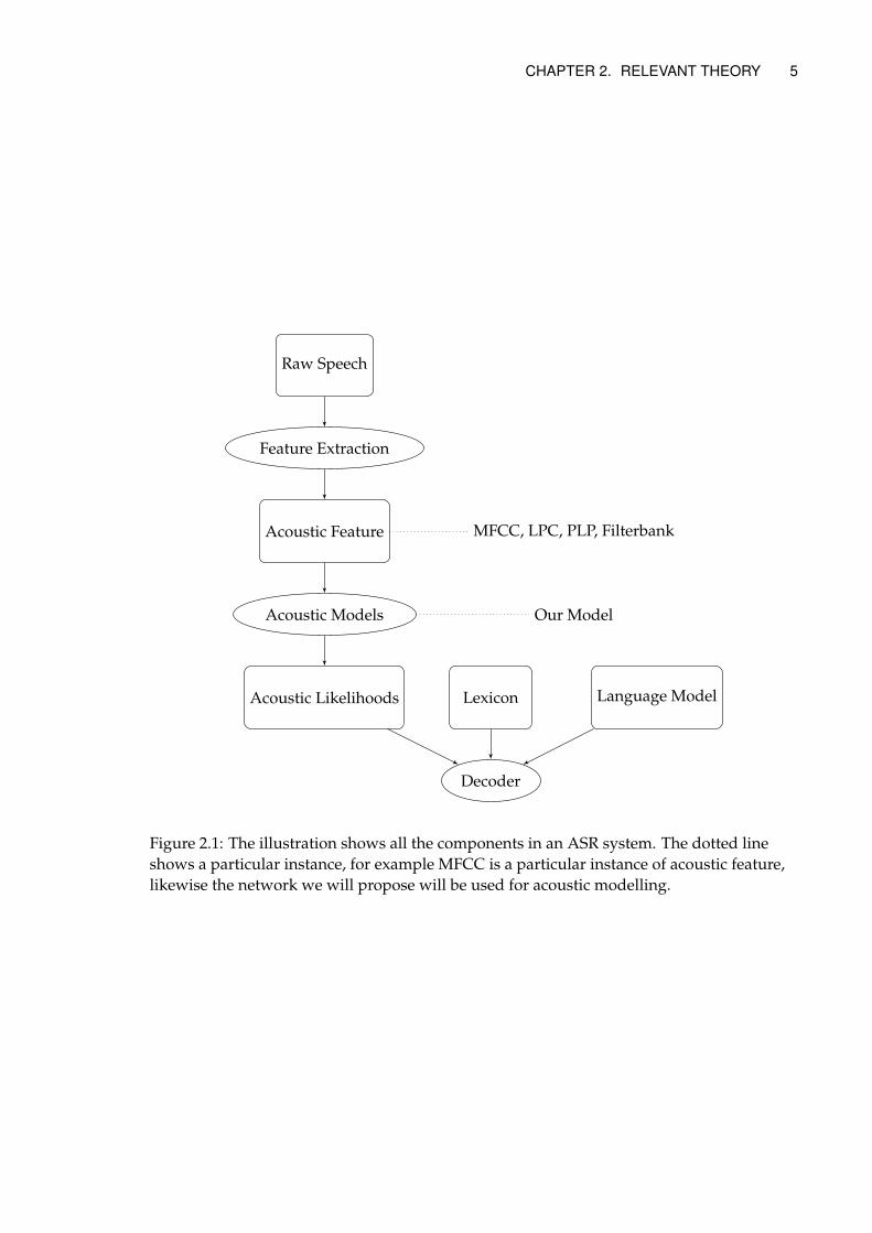
Figure 2.1 illustrates the processes involved with a typical speech recognizer. The differ-ent parts use a combination of signal processing and machine learning methods to tran-scribe a spoken utterance into a sequence of words. Because the problem is intrinsicallyaffected by uncertainty, a probabilistic framework is used.
First, the raw speech waveform is converted into a sequence X = x1, x2, ..., xT of fea-ture vectors spaced at regular time intervals. This process is called feature extraction and isbased on knowledge of speech production and perception. The goal of feature extractionis to convert speech into a representation that is suitable for the classification problem.More information about feature extraction methods is given in Section 2.2.
Given the sequence of observations X , the objective is to predict the most likely wordsequence W = w1, w2, ..., wm. In probabilistic terms this can be written as follows:
W = arg maxW
p(W |X), (2.1)
where p(W |X) is the posterior of the sequence of words W given the observation se-quence X . According to Bayes’ Rule, the above expression can be written as:
W = arg maxW
p(X|W )p(W )
p(X)(2.2)
= arg maxW
p(X|W )p(W ) (2.3)
The term p(W ) in the equation is our prior knowledge about which word sequencesare likely to occur in a language and in a specific task. This is called a language model.The term p(X|W ) in Eq. 2.2 is the likelihood of a sequence X of acoustic features givena particular sequence of words denoted by W . This is computed by acoustic and lexi-cal models. The lexical models describe word’s pronunciations in terms of sequences of
4
CHAPTER 2. RELEVANT THEORY 5
Raw Speech
Feature Extraction
Acoustic Feature MFCC, LPC, PLP, Filterbank
Acoustic Models Our Model
Acoustic Likelihoods Lexicon Language Model
Decoder
Figure 2.1: The illustration shows all the components in an ASR system. The dotted lineshows a particular instance, for example MFCC is a particular instance of acoustic feature,likewise the network we will propose will be used for acoustic modelling.
6 CHAPTER 2. RELEVANT THEORY
phonemes, and the acoustic models describe the likelihood of acoustic features givena certain phoneme. The decoder is a search algorithm that uses the information in theacoustic, lexical and language models to perform the maximization in Eq. 2.2.
The acoustic models are the main focus in this thesis. They encode knowledge aboutacoustics, phonetics, microphone, environment variability, and differences due to gender,accent, dialect and age of the speaker. In order to test the effects of the acoustic modelsalone on the speech recognition task, a slightly simplified task is considered: phone classi-fication. In this case, instead of the optimization in Eq. 2.1, we classify each feature framexn into one of K possible phonemic classes. The assessment of this classification task isonly reliable if the speech data is annotated at the phonetic level (as is the case for theTIMIT database used in this study). Acoustic models that perfrom better phone classi-fication are more likely to perform better speech recognition as well. Although phoneclassification is only the first step in estimating the method performance, this evaluationis an accepted practice when new speech recognition methods are introduced.
In the following sections, we will only describe feature extraction and acoustic mod-els, because the phone classification task considered in this thesis does not require lexicaland language models. We will focus in particular on Multi Layer Perceptrons and DeepNeural Networks that have been successfully used in recent years as acoustic models forspeech.
2.2 Feature Extraction
A speech waveform can be represented as a sequence of samples at a sampling rate thatcan typically vary between 8 and 20 kHz depending on the quality of the recording.The samples are highly correlated and contain variations that are not easily associatedwith phonetic classes without any preprocessing. The goal of feature extraction is to pro-vide a representation for the speech signal that is more suitable for classification. Sev-eral methods for feature extraction have been proposed in the past. The most commonlyused are based on a short time spectral representation of the signal, as, for example, MelFrequency Cepstral Coefficients (MFCCs) and Perceptual Linear Predictive coefficients(PLPs). In order to capture the time evolution of those feature vectors, first-order andsecond-order temporal differences are often appended to the original features.
MFCCs are calculated according to the procedure shown in Algorithm 1:
Algorithm 1 Procedure to calculate MFCCs
1: divide the signal into short, possibly overlapping frames2: For each frame, calculate the short time fourier transform3: Apply the (logarithmic) mel filterbank to power spectra, and take the sum of energy in
each filter.4: Calculate the logarithm of all filterbank energies5: Apply the Discrete Cosine Transform (DCT) of the log filterbank energies.6: Keep DCT coefficients 1-12 and discard the rest, energy coefficient is optional.7: Take the ∆ and ∆∆ of the coefficients w.r.t. preceding frames and append it to original
13 coefficients.
The first step is motivated by the assumption that, though time-varying, the speechsignal is stationary for short time intervals. The length of those intervals is typically be-
CHAPTER 2. RELEVANT THEORY 7
tween 10 and 20 msec. The frames are usually overlapping in time so that there is a smoothertransition in the information captured by two consecutive frames. The following stepsare motivated by perceptual phenomena. The cochlea is known to perform a frequencyanalysis of the signal, and humans are known to have logarithmic resolution both in fre-quency and in loudness. The Mel filterbank is a set of triangular filters, designed in sucha way that filters are logarithmically spaced in frequency.
The application of the Discrete Cosine Transform (DCT) is motivated by modellingconstraints. When the feature vectors are modelled by Gaussian Mixture Models (GMMs),it is desirable to work with uncorrelated features. This allows to greatly simplify themodels by using diagonal covariance matrices. This requirement has become less strin-gent with the advent of acoustic models based on neural networks (NNs), because thesemodels can easily cope with feature correlations. In fact, in NN acoustic modelling it iscommon to work with filterbank features directly, that is, to skip steps number 5 and 6 inAlgorithm 1 [8, 41].
The reason for truncating the MFCC vector to only 12 components is to limit the rep-resentation to a coarse description of the speech spectra, because the details are related tothe frequency of vibration of the vocal fold and, in a first approximation, are a disturbingfactor in phone classification.
This approach of knowledge driven pre-processing of the waveform has proved to besuccessful in discarding information that is irrelevant for discrimination. However, it isalways possible that relevant information is lost in the process. In some very recent stud-ies [1], Convolutional Neural Networks have been applied to the speech samples directly,eliminating the need for feature extraction. Although more difficult to train, these modelscan potentially make use of all the information contained in the signal. This similar trendcan be observed in Computer Vision as well [21].
2.3 Acoustic Modelling
Hidden Markov Models (HMMs) are the most popular statistical models in Speech Recog-nition. A first-order Markov chain is a state-space model, where the probability distribu-tion of the current state depends only on the previous state. A Hidden Markov modelis more complex in the way that the state is not directly observable. We observe an out-put that, given the current state, is conditionally independent from previous outputs andstates. The states follow a first-order Markov chain. In speech recognition, the sequencesof observations correspond to the feature vectors described in the previous section. Thestates roughly correspond to phonetic units.
The model defines two types of probability distributions: transition probabilities, whichdescribe what state is more likely to occur in the next step given the current state, andemission probabilities which describe the likelihood of a specific observation given the cur-rent state. One important inference problem is to calculate the posterior probability of thephoneme states, given a sequence of acoustic observations.
The emission probabilities, for continuous feature vectors (e.g. MFCCs) are in ASRusually modelled by Gaussian Mixture Models. The combined model is called GMM-HMM. GMMs have been state-of-the-art emission probability models in ASR for manyyears, mainly due to their flexibility. Closed form adaptation techniques such as Max-imum likelihood linear regression (MLLR) [29] and feature-based MLLR (fMLLR) [11],made it possbile to quickly adapt those models to new speakers or environmental situa-
8 CHAPTER 2. RELEVANT THEORY
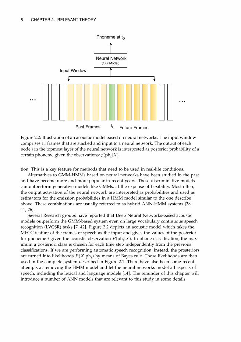
Figure 2.2: Illustration of an acoustic model based on neural networks. The input windowcomprises 11 frames that are stacked and input to a neural network. The output of eachnode i in the topmost layer of the neural network is interpreted as posterior probability of acertain phoneme given the observations: p(phi|X).
tion. This is a key feature for methods that need to be used in real-life conditions.Alternatives to GMM-HMMs based on neural networks have been studied in the past
and have become more and more popular in recent years. These discriminative modelscan outperform generative models like GMMs, at the expense of flexibility. Most often,the output activation of the neural network are interpreted as probabilities and used asestimators for the emission probabilities in a HMM model similar to the one describeabove. These combinations are usually referred to as hybrid ANN-HMM systems [38,41, 26].
Several Research groups have reported that Deep Neural Networks-based acousticmodels outperform the GMM-based system even on large vocabulary continuous speechrecognition (LVCSR) tasks [7, 42]. Figure 2.2 depicts an acoustic model which takes theMFCC feature of the frames of speech as the input and gives the values of the posteriorfor phoneme i given the acoustic observation P (phi|X). In phone classification, the max-imum a posteriori class is chosen for each time step independently from the previousclassifications. If we are performing automatic speech recognition, instead, the prosteriorsare turned into likelihoods P (X|phi) by means of Bayes rule. Those likelihoods are thenused in the complete system described in Figure 2.1. There have also been some recentattempts at removing the HMM model and let the neural networks model all aspects ofspeech, including the lexical and language models [14]. The reminder of this chapter willintroduce a number of ANN models that are relevant to this study in some details.
CHAPTER 2. RELEVANT THEORY 9
2.4 MLPs and Deep Neural Networks
As our model is an autoencoder, a kind of a neural network, we will first describe a sim-ple MLP and then autoencoders more specifically. A Multi Layer Perceptron (MLP), alsocalled feedforward neural network, is a series of logistic regression models stacked ontop of each other. In each layer, the inputs are linearly combined and the combination ispassed through a non-linear function. A basic MLP is made up of three layers, the firstlayer is the input layer. The number of nodes in the input layer is equal to the dimensionof the input. The second layer is called the "hidden layer", because of not being observeddirectly. The output layer is used to perform classification or regression. The dimensionof the output is equal to the number of classes for classification or to the dimensionalityof the output signal for regression. There may be more than one hidden layers in MLPs.Models with several hidden layers are often called Deep Neural Networks (DNNs).
In a fully connected network, all the nodes in one layer are connected to all the nodesof the next layers. A connection between a node in one layer to a node in the next layeris assigned a weight, wij . The activation of a node from the second to the last layer isa non-linear function applied to the weighted sum of all nodes from the previous layer.This non-linear function is also called as an activation function. The expression both inscalar form and matrix form is given in 2.4 and 2.5
yj = f
(∑i
wijxi + bj
)(2.4)
y = f(W Tx + b), (2.5)
where x is the activation of layer n, or the input vector for the input layer, y is the out-put of layer n + 1, b is the bias value of the hidden layer and W is the weight matrixbetween the layers.
The activation functions can vary depending on the position of the node in the net-work. For hidden layers, commonly used activation functions are, for example:
1. Sigmoid function :
yj =1
(1 + e−zj )(2.6)
2. Hyperbolic tangent function :yj = tanh(zj) (2.7)
3. Rectified Linear Unit (ReLu) function [34]:
yj = max(xj , 0) (2.8)
where zj =∑
iwijxi + bj is the linear combination of the activations of all nodes con-nected to node j.
For the output layer, the activation function depends on the task. Linear activation iscommon for regression, whereas for classification it is common to use softmax activations,given by
yj =exp(zj)∑k exp(zk)
(2.9)
10 CHAPTER 2. RELEVANT THEORY
Because the activations sum to 1, they can be interpreted as posterior probabilities of thedifferent classes given the input to the network. The maximum a posteriori classifier isthen implemented by selecting the class that corresponds to the maximum activation:
o = arg maxjyj (2.10)
DNNs are generally discriminatively trained using the Backpropagation algorithm tominimise a cost function. Backpropagation is an algorithm to train a multi-layered net-work so that each layer in the architecture can learn a mapping from input to output thatis optimal according to an optimality criterium. The Backpropagation Learning algorithmrequires an input and a target. First the weights in the network are initialized to randomvalues. In the forward pass, an observation is input to the network and activations aregenerated for each node in each layer based on the current values of the weights. Thisallows us to measure the difference between the output of the network y and the desired(target) output t. This measurement can be a simple square error on one single observa-tion
EE =1
2(t− y)2 (2.11)
or a cross entropy loss measure computed over several observations:
EC = − 1
n
n∑i=1
K∑j=1
[ti log yij + (1− ti)log(1− yij)
], (2.12)
where the summation over j corresponds to the nodes in the output layer, and the sumover i is an average over a number of observations.
In the backward pass, we calculate how the output error is dependent on each weightin the network, and update the weights in order to minimize the error. This is achievedby factorizing the partial derivatives with the help of the chain rule. This way, we canpropagate the deltas back from the ouput layer to the input. If we evaluate the depen-dency of the error on a specific weight wij as ∂E
∂wijand we start from the value of the
weight wij(t) at iteration t, the new value of the weight at iteration t + 1 is calulated bygradient descent as:
wij(t+ 1) = wij(t) + ∆wij(t+ 1) (2.13)
= wij(t)− η∂E
∂wij(2.14)
where η is the learning rate.For very large datasets, calculating the gradient for the entire dataset at once could
be extremely computationally intensive. To mitigate this problem, it is more efficient tocompute the derivatives on a small, random mini batch of training points, and then theweights of the layer are modified proportional to the gradient. To remove the effect ofnoisy spurious training samples, it is common to use an additional momentum term inthe training algorithm to make the training more uniform and less spiky. The weight up-date rule including the momentum term α is given by
∆wij(t) = α∆wij(t)− η∂E
∂wij. (2.15)
CHAPTER 2. RELEVANT THEORY 11
The term α ensures smoother variations in gradient values. The term η gives the learningrate. DNNs with many hidden layers and many units per layer are very flexible modelswith a very large number of parameters, which can easily overfit due to some spuriouscharacteristic of the training set. To reduce overfitting, several techniques like L2 regular-isation or Drop-out are used, which penalise the magnitude of the weights, and preventthem from becoming very large.
2.5 Autoencoders
Multi layer perceptrons require the target value to be specified for each training example.If we do not have this information, we can still learn a representation that is dependenton the distribution of the data by means of an auto-encoder. An auto-encoder is specialkind of neural network with two components: an encoder and a decoder. The encodertakes the input x, and maps it to a hidden representation y, which is given by
y = σ(Wx+ bh). (2.16)
The latent or hidden representation y is mapped back to the original input, using a de-coder which is given as:
z = σ(W’y + bv) (2.17)
where y is the encoded value, y is a possibly corrupted version of the the encoded value,bh, bv are the bias values of encoder and decoder respectively, W is the weight matrix ofthe encoder, while W ′ represents its transpose. This network tries to minimise the recon-struction error given as:
LC(x, z) = ||x− z||2 (2.18)
LB(x, z) = −d∑
k=1
[xk log zk + (1− xk) log(1− zk)] (2.19)
The first equation 2.18 is for continuous input, while the second equation 2.19 is used forclasses and binary vectors. It is basically the cross-entropy error already defined above.Although we have expressed the equations with σ function, the activation function couldbe any other prominent activation functions.
If the hidden layer of the auto-encoder has a lower dimensionality than the input, themodel will perform non-linear dimensionality reduction. If it is of equal or greater di-mensionality, special care must be put to avoid that the model learns a trivial mapping(identity function). For this reason, the input or the hidden representations may be cor-rupted during training.
2.5.1 Manifold Learning with Autoencoders
A reason as to why auto-encoders do so well is that they exploit the idea that data isgenerally concentrated around a manifold, or several subsets of manifolds. The theoreti-cal understanding about how auto-encoders map data manifolds is still a very active areaof research. But to give a brief motivation, the general principle behind all autoencodersis a trade-off between two ideas: first, to learn a representation y of a training examplex such that x can be approximately recovered from y through a decoder. x should be
12 CHAPTER 2. RELEVANT THEORY
x
z
x
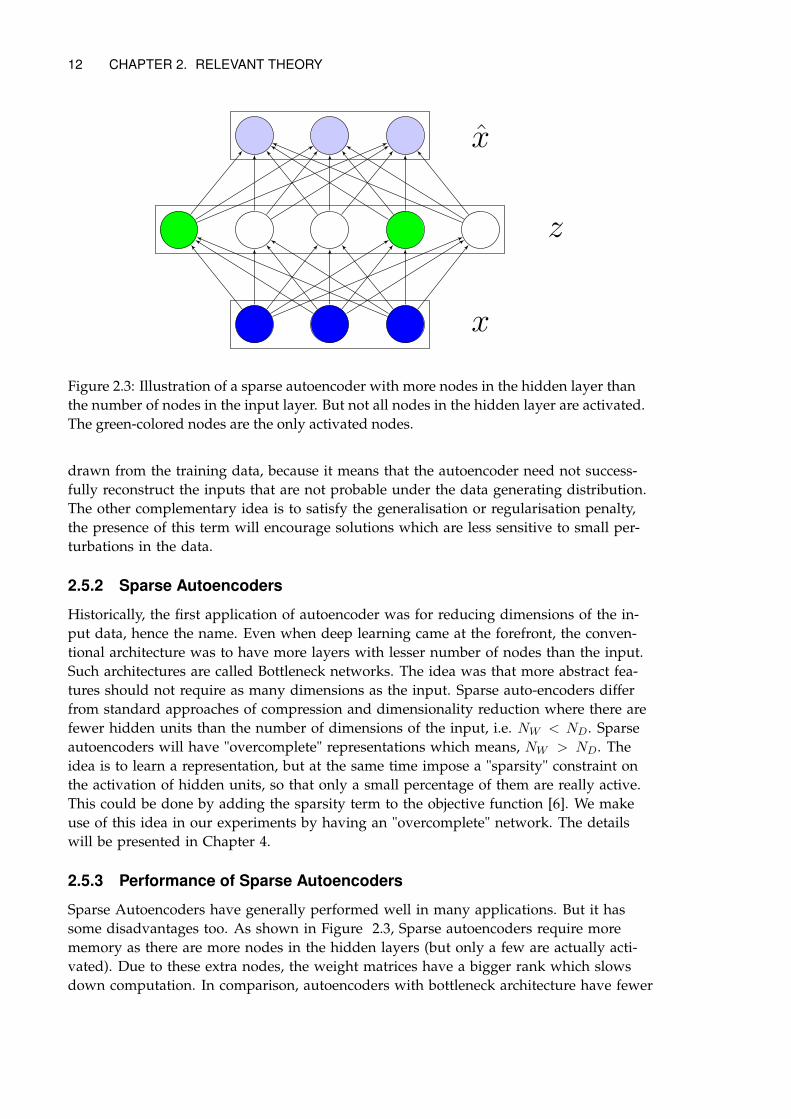
Figure 2.3: Illustration of a sparse autoencoder with more nodes in the hidden layer thanthe number of nodes in the input layer. But not all nodes in the hidden layer are activated.The green-colored nodes are the only activated nodes.
drawn from the training data, because it means that the autoencoder need not success-fully reconstruct the inputs that are not probable under the data generating distribution.The other complementary idea is to satisfy the generalisation or regularisation penalty,the presence of this term will encourage solutions which are less sensitive to small per-turbations in the data.
2.5.2 Sparse Autoencoders
Historically, the first application of autoencoder was for reducing dimensions of the in-put data, hence the name. Even when deep learning came at the forefront, the conven-tional architecture was to have more layers with lesser number of nodes than the input.Such architectures are called Bottleneck networks. The idea was that more abstract fea-tures should not require as many dimensions as the input. Sparse auto-encoders differfrom standard approaches of compression and dimensionality reduction where there arefewer hidden units than the number of dimensions of the input, i.e. NW < ND. Sparseautoencoders will have "overcomplete" representations which means, NW > ND. Theidea is to learn a representation, but at the same time impose a "sparsity" constraint onthe activation of hidden units, so that only a small percentage of them are really active.This could be done by adding the sparsity term to the objective function [6]. We makeuse of this idea in our experiments by having an "overcomplete" network. The detailswill be presented in Chapter 4.
2.5.3 Performance of Sparse Autoencoders
Sparse Autoencoders have generally performed well in many applications. But it hassome disadvantages too. As shown in Figure 2.3, Sparse autoencoders require morememory as there are more nodes in the hidden layers (but only a few are actually acti-vated). Due to these extra nodes, the weight matrices have a bigger rank which slowsdown computation. In comparison, autoencoders with bottleneck architecture have fewer
CHAPTER 2. RELEVANT THEORY 13
nodes in the hidden layer and could possibly have lesser time complexity. The over-all time complexity of the neural network is linear in the number of total connectionspresent and though a sparse autoencoder might have much more connections than a bot-tleneck autoencoder, many of which might not even be used after the first few iterations.So, it is more difficult to find a lower bound on the time complexity for sparse autoen-coders. Sparse autoencoders could offer more flexibility and additional modelling powerthan a bottleneck autoencoder, although the theoretical understanding of their working isstill an active area of research.
2.5.4 Applications of Autoencoders
Autoencoders have been successfully applied to dimensionality reduction and informa-tion retrieval tasks. Dimensionality Reduction, infact was the first application of repre-sentation learning and auto-encoders. One other task that has made successful use ofautoencoders is information retrieval, where the dimensionality reduction algorithm pro-duces a low dimensional and binary code, which can be then stored in a hash table map-ping binary code to entries for fast search. The hash table gives us the capability to per-form information retrieval by returning all database entries having the same binary code.The search is then a lot faster because it is done on "hashed" binary codes.
2.6 Semi-Supervised Learning
While in the above sections, we talked about one popular supervised learning modeland one unsupervised learning model section, in this section we will talk about Semi-Supervised Learning. Semi-Supervised Learning is a field of study in machine learningwhich falls between "supervised" learning (a problem of classification/regression withfull classes labels available in the training data) and unsupervised learning (modellingof input data into classes without any class labels). In most practical applications, it ishard to get fully labeled training data. Unlabeled training data is generally easier and insome cases much cheaper to obtain. Then an interesting question which arises is, howcan the unlabeled data be used in conjunction with labeled data to improve the accuracyof a system trained on just the labeled data. If it can be, what is the minimum relativeproportion at which the unlabeled data will lose any relevance to the problem. We aregiven a set of independent and identically distributed input samples, x1, ..., xl ∈ X , andtheir corresponding targets: y1, ..., yl ∈ Y such that DL = (XL, YL). In addition we alsohave u unlabeled input samples, xl+1, xl+2, ..., xl+u ∈ Xu, such that DU = (XU ), the totalnumber of samples is then given as n = l + u. Supervised classification only utilizes theinformation from DL to learn a decision boundary, whereas in semi-supervised learningframework, the decision boundary is obtained by utilizing information from both DL andDU at the same time. Semi-supervised Learning attempts to make use of this combineddataset D = DL ∪DU to surpass the classification performance that can be obtained eitherby doing supervised learning (discarding unlabeled data) or doing unsupervised learningsuch as clustering (discarding labeled information). Some researchers refer SSL as "trans-ductive learning" or "inductive learning". The goal of transductive learning would be toinfer the correct labels of the unlabeled dataset DU .

14 CHAPTER 2. RELEVANT THEORY
2.7 Assumptions
We make several assumptions in SSL, the key idea for semisupervised learning to workis that, the information about distribution p(x) which can be obtained from unlabeleddata should also carry the information required for inference of y expressed throughp(y|x).
Chapter 3
Related Work
In this chapter, we will talk about existing literature on the application of deep neuralnetworks for ASR and on Semi-Supervised Learning techniques. One prominent suchtechnique is Graph Based Semi-Supervised Learning (GBL SSL).
3.1 Deep Neural Networks in ASR
This section introduces us to the kind of DNNs and different architectures, which havebeen recently used in ASR.
3.1.1 Deep Belief Networks
The first set of results which beat traditional GMM-HMMs were reported by [38], wherethe authors trained DBNs (Deep Belief Networks) for recognising the HMM states ofphonemes, given an input of 9-11 frames of MFCC feature vectors. A DBN contains sev-eral stacked layers of RBMs (Restricted Boltzmann Machine). The RBMs are generativelytrained using the contrastive divergence algorithm outlined in [38]. Initially, the resultswere reported on TIMIT [10]. Further attempts were made to replicate the success ofTIMIT on large scale vocabulary applications. The first such attempt was on data col-lected from Bing mobile voice search application (BMVS). It had about 24 hours of train-ing data with high degree of variability. The DBNs trained on this dataset achieved sen-tence accuracy of 69.6% on the test set compared to just 63.8% achieved by the traditionalGMM-HMM baseline. The DBNs are a kind of unsupervised learning model, and theywere popular as a way to pretrain a neural network. But Further research revealed thatpurely supervised learning of a DNN works comparably, provided a large amount of la-beled data is available, the initial weights are set carefully, and the mini-batch sets are setproperly [43]. Since then, DBNs have fallen a little out of favour in the speech commu-nity as the overhead of pretraining can be replaced by careful tuning of the network.
3.1.2 Recurrent Neural Networks
Recurrent Neural Networks (RNNs) are another kind of neural network with an abilityto model temporal and sequential data. While the above mentioned DBNs is a modelfor unsupervised learning, RNN is purely supervised training. One major advantagewith RNNs is that they do not require fixed input feature length like the above discussedfeed-forward networks. The experiments described in [14], demonstrate how RNNs can
15
16 CHAPTER 3. RELATED WORK
be made to understand multiple levels of representation, a salient feature of deep nets,and combine it with their ability to make flexible use of long range context in ASR. Theauthors reported a test set WER (word error rate) of 17.7%, which beat all the previ-ous benchmarks. RNNs have earlier been used with HMMs, but this is the first instancewhen RNNs have been used from end to end, and proved that stacking multiple recur-rent layer each on top of the other can give better results just like their counterparts indeep feed forward networks.
3.2 Examples of Semi-Supervised Learning Methods
This section introduces us to the different kinds of SSL techniques. The model we usein this thesis falls in the last category of models: Semi Supervised Learning by Autoen-coder.
3.2.1 Heuristic based SSL/Self-Training
Among all the existing and accepted techniques, the simplest algorithm for semi-supervisedlearning is based on "self-training" scheme, where a model is trained just with the la-beled part of dataset, and newly labeled data obtained from its own highly confidentpredictions, until the confidence level of the predictions drops below a certain thresh-old. The training can take several iterations. To state formally, the self-training approachstarts with the labeled set L = {(xi, yi)li=1} and unlabeled set U = {(xi)ni=l+1}. An ini-tial model f is trained using only the labeled data using standard supervised learning.The resulting model is then used to make predictions on U , where the most confidentpredictions are removed from U and added to L together with their corresponding classpredictions. In the next iteration, the model is refined with the new augmented set L. Acritical assumption made in this algorithm is that the predictions added to the initial la-beled set are reliable enough themselves. One big advantage of this approach is that itcan be used as a wrapper for any learning algorithm.
This is quite a general technique, which has been used in many different research aressuch as object classification [40] and speech recognition. In [46, 15, 17], self-training wasused in combination with neural networks, whereas in [24, 25, 47] in combination withGMM-based acoustic models. Although showing promising results, these methods in-volve heuristics and can reinforce "bad" predictions. The confidence level and unit selec-tion are very important in these models and any mistuning of these parameters can leadto bad results in later iterations.
3.2.2 Transductive SVMs
Transductive SVMs [18] work on the the principle of avoiding having decision bound-aries, where input is heavily distributed. Putting a decision boundary in high density re-gions of input, increases the chances of getting "all predictions wrong", this idea is basedon the cluster smoothness, which was discussed in the previous section. TransductiveSupport Vector Machines (TSVMs) is an extension of traditional SVMs with unlabeleddata. They have the same objective of maximising margin between classes, while ensur-ing that there are few unlabeled examples near the margin. Finding the exact solution isNP-hard. Some efficient approximate algorithms have been proposed but they lack scala-bility to problems with very large datasets.
CHAPTER 3. RELATED WORK 17
3.2.3 Entropy Based Semi Supervised Learning
Entropy based Learning jointly model the labeled and unlabeled data. The primary mo-tivation is entropy minimization for these methods and has been proposed in [9, 16].In [16], the authors proposed to jointly model the labeled and unlabeled data in a con-ditional entropy minimisation framework first demonstrated in [13]. The authors alsomaximised the conditional entropy regularisation term posed on the unlabeled data, inaddition to the usual task of maximising the posteriors on the labeled data. This addi-tional regularizer encourages the model to have as great confidence as possible on labelprediction of the unlabeled data. The optimisation of the framework was performed us-ing the extended Baum-Welch algorithm. The method was evaluated on different speechrecognition tasks such as phonetic classification and phonetic recognition tasks, wheresome improvement was obtained on the TIMIT dataset compared to a supervised dis-criminatively trained GMM model with Maximum Mutual Information Criterion [37].These methods have mostly been applied with GMM models in the literature, and thereis further scope for their study in discriminative methods and could be a potential areaof future study.
3.2.4 Graph based SSL
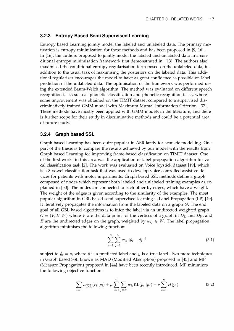
Graph based Learning has been quite popular in ASR lately for acoustic modelling. Onepart of the thesis is to compare the results achieved by our model with the results fromGraph based Learning for improving frame-based classification on TIMIT dataset. Oneof the first works in this area was the application of label propagation algorithm for vo-cal classification task [2]. The work was evaluated on Voice Joystick dataset [19], whichis a 8-vowel classification task that was used to develop voice-controlled assistive de-vices for patients with motor impairments. Graph based SSL methods define a graphcomposed of nodes which represent both labeled and unlabeled training examples as ex-plained in [50]. The nodes are connected to each other by edges, which have a weight.The weight of the edges is given according to the similarity of the examples. The mostpopular algorithm in GBL based semi supervised learning is Label Propagation (LP) [49].It iteratively propagates the information from the labeled data on a graph G. The endgoal of all GBL based algorithms is to infer the label via an undirected weighted graphG = (V,E,W ) where V are the data points of the vertices of a graph in DL and DU , andE are the undirected edges on the graph, weighted by wij ∈ W . The label propagationalgorithm minimises the following function:
n∑i=1
n∑j=1
wij ||yi − yj ||2 (3.1)
subject to yi = yi where y is a predicted label and y is a true label. Two more techniquesin Graph based SSL known as MAD (Modified Absorption) proposed in [45] and MP(Measure Propagation) proposed in [44] have been recently introduced. MP minimizesthe following objective function:
l∑i=1
DKL(ri||pi) + µ
n∑i=1
∑j∈N
wijKL(pi||pj)− νn∑i=1
H(pi) (3.2)
18 CHAPTER 3. RELATED WORK
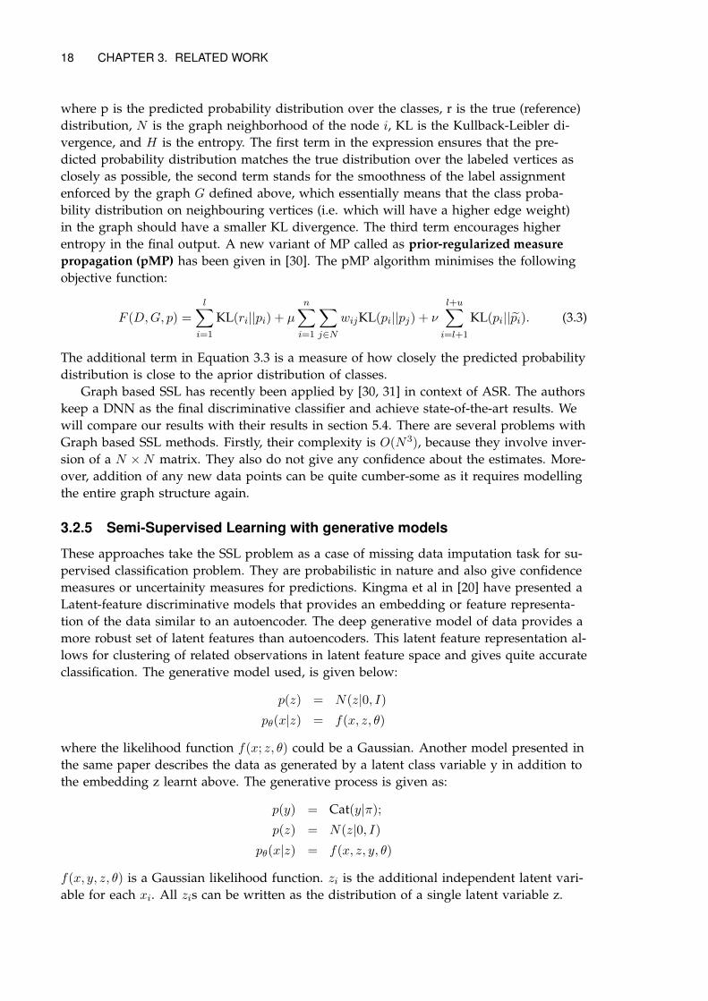
where p is the predicted probability distribution over the classes, r is the true (reference)distribution, N is the graph neighborhood of the node i, KL is the Kullback-Leibler di-vergence, and H is the entropy. The first term in the expression ensures that the pre-dicted probability distribution matches the true distribution over the labeled vertices asclosely as possible, the second term stands for the smoothness of the label assignmentenforced by the graph G defined above, which essentially means that the class proba-bility distribution on neighbouring vertices (i.e. which will have a higher edge weight)in the graph should have a smaller KL divergence. The third term encourages higherentropy in the final output. A new variant of MP called as prior-regularized measurepropagation (pMP) has been given in [30]. The pMP algorithm minimises the followingobjective function:
F (D,G, p) =
l∑i=1
KL(ri||pi) + µ
n∑i=1
∑j∈N
wijKL(pi||pj) + ν
l+u∑i=l+1
KL(pi||pi). (3.3)
The additional term in Equation 3.3 is a measure of how closely the predicted probabilitydistribution is close to the aprior distribution of classes.
Graph based SSL has recently been applied by [30, 31] in context of ASR. The authorskeep a DNN as the final discriminative classifier and achieve state-of-the-art results. Wewill compare our results with their results in section 5.4. There are several problems withGraph based SSL methods. Firstly, their complexity is O(N3), because they involve inver-sion of a N ×N matrix. They also do not give any confidence about the estimates. More-over, addition of any new data points can be quite cumber-some as it requires modellingthe entire graph structure again.
3.2.5 Semi-Supervised Learning with generative models
These approaches take the SSL problem as a case of missing data imputation task for su-pervised classification problem. They are probabilistic in nature and also give confidencemeasures or uncertainity measures for predictions. Kingma et al in [20] have presented aLatent-feature discriminative models that provides an embedding or feature representa-tion of the data similar to an autoencoder. The deep generative model of data provides amore robust set of latent features than autoencoders. This latent feature representation al-lows for clustering of related observations in latent feature space and gives quite accurateclassification. The generative model used, is given below:
p(z) = N(z|0, I)
pθ(x|z) = f(x, z, θ)
where the likelihood function f(x; z, θ) could be a Gaussian. Another model presented inthe same paper describes the data as generated by a latent class variable y in addition tothe embedding z learnt above. The generative process is given as:
p(y) = Cat(y|π);
p(z) = N(z|0, I)
pθ(x|z) = f(x, z, y, θ)
f(x, y, z, θ) is a Gaussian likelihood function. zi is the additional independent latent vari-able for each xi. All zis can be written as the distribution of a single latent variable z.
CHAPTER 3. RELATED WORK 19
3.3 Autoencoder Based Semi-Supervised Learning
This section introduces us to the model we are going to present and motivate about it.Deep Neural Networks are generally trained either from just fully labeled data, or fromjust purely unlabeled data. Both models, when used alone are not ideal. Ranzato et al.in [39] explored the possibility of having a joint objective made of both a supervised andunsupervised objective on documents where bag of word representations were used asinput features. The authors performed their experiments on Reuters and Newsgroupsdatasets. We propose to use a similar approach to frame-based phoneme recognition inASR. Although our objective function is the same as the one proposed in [39], our setup is different in a number of ways. Firstly, instead of the compact and lower dimen-sional encoding used in [39], we employ sparse encoding. Secondly, instead of stackinga number of encoders, decoders and classifiers in a deep architecture as in [39], we usea single layer model. This is motivated by work in [6], where the authors analyse theeffect of several model parameters in unsupervised learning of neural networks on com-puter vision benchmark data sets such as CIFAR-10 and NORB. They conclude that state-of-the-art results can be achieved with single layer networks regardless of the learningmethod, if an optimal model setup is chosen. An introduction to sparse autoencoders canbe found in Stanford Lecture notes given by Andrew NG [35].
Chapter 4
Method
We present our algorithm here. We will try to motivate it from our understanding ofautoencoders and the principles of supervised classification. Neural Networks requireproper-care and attention during training, so we will describe how to initialise the net-work and the practical details to be kept in mind, and the hyperparameter values weused. We will also try to explain why we made certain choices in the network config-uration. We will also describe Gradient Checking, which is an important technique fordebugging Backpropagation in Neural Networks.
4.1 The Model
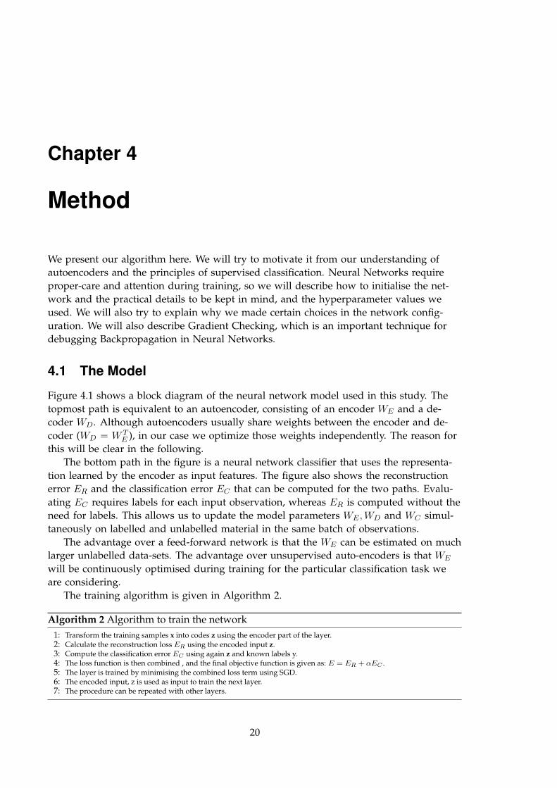
Figure 4.1 shows a block diagram of the neural network model used in this study. Thetopmost path is equivalent to an autoencoder, consisting of an encoder WE and a de-coder WD. Although autoencoders usually share weights between the encoder and de-coder (WD = W T
E ), in our case we optimize those weights independently. The reason forthis will be clear in the following.
The bottom path in the figure is a neural network classifier that uses the representa-tion learned by the encoder as input features. The figure also shows the reconstructionerror ER and the classification error EC that can be computed for the two paths. Evalu-ating EC requires labels for each input observation, whereas ER is computed without theneed for labels. This allows us to update the model parameters WE ,WD and WC simul-taneously on labelled and unlabelled material in the same batch of observations.
The advantage over a feed-forward network is that the WE can be estimated on muchlarger unlabelled data-sets. The advantage over unsupervised auto-encoders is that WE
will be continuously optimised during training for the particular classification task weare considering.
The training algorithm is given in Algorithm 2.
Algorithm 2 Algorithm to train the network1: Transform the training samples x into codes z using the encoder part of the layer.2: Calculate the reconstruction loss ER using the encoded input z.3: Compute the classification error EC using again z and known labels y.4: The loss function is then combined , and the final objective function is given as: E = ER + αEC .5: The layer is trained by minimising the combined loss term using SGD.6: The encoded input, z is used as input to train the next layer.7: The procedure can be repeated with other layers.
20
CHAPTER 4. METHOD 21
x WE tanh WD tanh ER +
WC softmax EC
E
t
x
z x
y α
encoder decoder
classifier
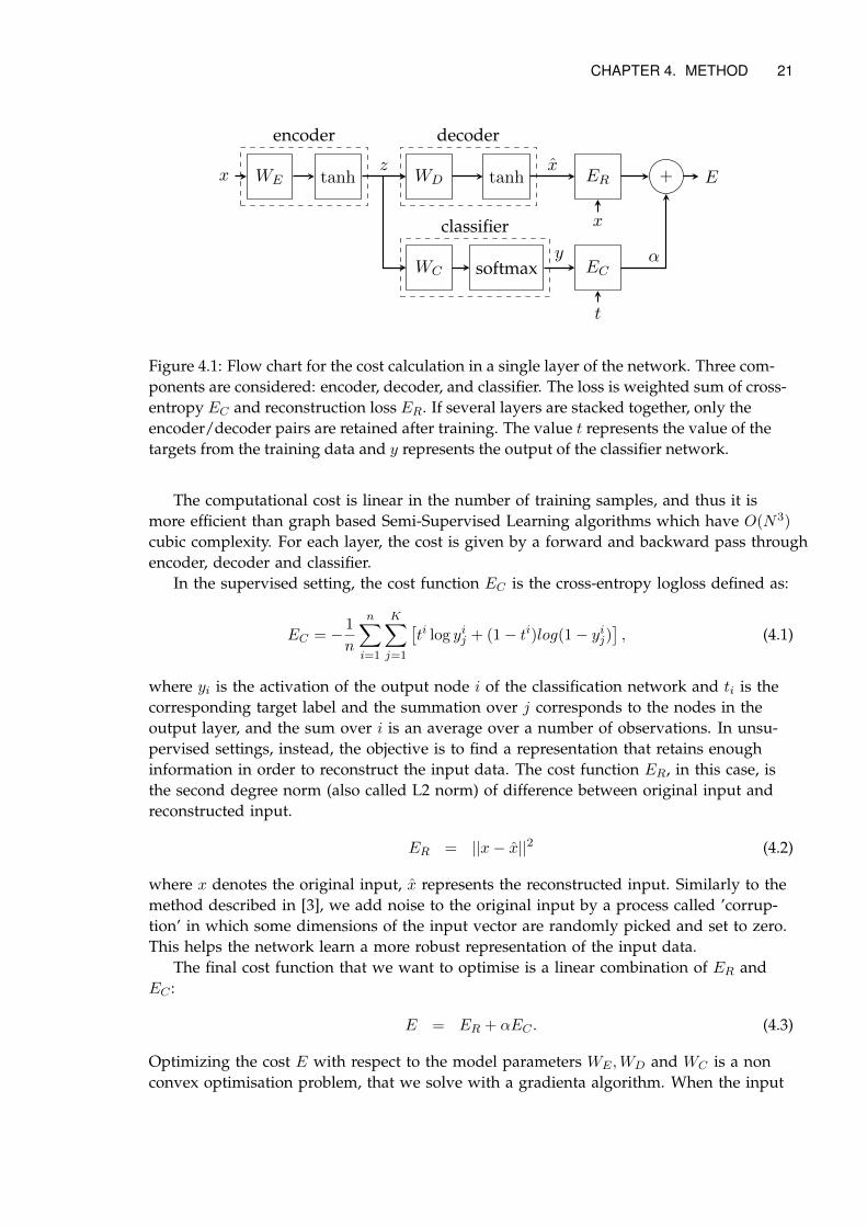
Figure 4.1: Flow chart for the cost calculation in a single layer of the network. Three com-ponents are considered: encoder, decoder, and classifier. The loss is weighted sum of cross-entropy EC and reconstruction loss ER. If several layers are stacked together, only theencoder/decoder pairs are retained after training. The value t represents the value of thetargets from the training data and y represents the output of the classifier network.
The computational cost is linear in the number of training samples, and thus it ismore efficient than graph based Semi-Supervised Learning algorithms which have O(N3)
cubic complexity. For each layer, the cost is given by a forward and backward pass throughencoder, decoder and classifier.
In the supervised setting, the cost function EC is the cross-entropy logloss defined as:
EC = − 1
n
n∑i=1
K∑j=1
[ti log yij + (1− ti)log(1− yij)
], (4.1)
where yi is the activation of the output node i of the classification network and ti is thecorresponding target label and the summation over j corresponds to the nodes in theoutput layer, and the sum over i is an average over a number of observations. In unsu-pervised settings, instead, the objective is to find a representation that retains enoughinformation in order to reconstruct the input data. The cost function ER, in this case, isthe second degree norm (also called L2 norm) of difference between original input andreconstructed input.
ER = ||x− x||2 (4.2)
where x denotes the original input, x represents the reconstructed input. Similarly to themethod described in [3], we add noise to the original input by a process called ’corrup-tion’ in which some dimensions of the input vector are randomly picked and set to zero.This helps the network learn a more robust representation of the input data.
The final cost function that we want to optimise is a linear combination of ER andEC :
E = ER + αEC . (4.3)
Optimizing the cost E with respect to the model parameters WE ,WD and WC is a nonconvex optimisation problem, that we solve with a gradienta algorithm. When the input
22 CHAPTER 4. METHOD
datapoint is not accompanied by a label, the classifier part of the layer is not updated,and the loss function simply reduces to ER.
The data is split into three sets. The optimization is performed on the training set,while a validation set is used to optimize the meta parameters for each run, for exam-ple the value of α in the linear combination of Eq. 4.3. Neural Networks contain manyhyperparameters and tuning could be a challenge.
The final results are given on an independent test set.As we will describe later in 5.1, we run experiments on two datasets: MNIST and
TIMIT. In case of MNIST, the input x is the raw image represented by the pixels con-catenated row-wise into a single vector. The output y is the digit number (0-9). In caseof TIMIT, the input x is the MFCC+ ∆ + ∆∆ feature concatenated together with the fea-tures of 5 previous and 5 next frames as in Figure 2.2. The procedure to obtain these fea-tures has already been explained in Section 2.2 The output y are all the possible speechphonemes. Please note, that recently, it is more prevalent to have senones or the hmmstates of the phonemes as the target labels as in [38], but to compare with other tech-niques in Semi-supervised learning for speech [30, 2], we experimented with phonemes.
The training in this model can be peformed greedly layer by layer if we wish to usedeep networks. However, in our experiments, we use only a single layer for feature rep-resentation.
We use mini-batch SGD as explained in the theory section as the optimizer over thiscost function. The weight matrices, WC and WD are simply updated by normal back-propagation algorithm as shown in the equations 2.14 given in the Theory section. How-ever, the update of the encoder weight matrix is not straightforward as in the other two,and is given by:
∂E
∂WE=∂ER∂WE
+ α∂EC∂WE
(4.4)
WE = WE − η∂E
∂WE. (4.5)
It is important to note that the update of encoder weight WE is dependent both onWD and WC , and the delta propagated in the backpropagation algorithm will be a linearcombination of the deltas calculated in both parts. Because of its sparse properties, wecall this model Semi-Supervised Sparse Autoencoder (SSSAE). The weight update givenin Equation 4.5 was implemented using Theano [23] library.
4.2 Evaluation
The evaluation method was simply classification accuracy given as proportion of cor-rectly classified examples. In machine learning experiments, the standard convention isto partition the data into three sets: training set, validation set, and a test set. The largestof them is the training set, which is used to train the model, or fitting parameters of amodel. When given a model class and a choice of hyperparameters, the parameters areselected which give the minimum error on the training set. Given a type of model, onetunes the hyperparameters on the validation set. The test set is kept untouched dur-ing the entire training process. Finding the error on the test set is the last step. We per-formed experiments on two different datasets. In the MNIST problem, each example
CHAPTER 4. METHOD 23
correspond uniquely to a class (written digit) and the classification accuracy is straight-forward to define. In ASR, however, this is not the case. Because the speech signal is acontinuous stream of linguistic units, many metrics can be defined at different levels ofdetails. We can compute errors at the phonetic level, or word level or even at the levelof full sentences. We can also consider fine alignment of the recognized linguistic unitsin time, or just consider the sequence of linguistic units disregarding errors in alignment.Which metric we use is determined by the application and by the output of our speechrecognizer. The most commonly used metric is called Word Error Rate (WER). This met-ric is defined on sequences of words and disregards the alignment in time. The sequenceof recognized words is aligned with the sequence of labels by means of dynamic pro-gramming, and the mismatch is computed in terms of number of insertions, deletions orsubstitutions. In this thesis, however, we focus on phone recognition, and we thereforeuse a corresponding metric. The most common way to calculate accuracy at the phoneticlevel is to consider each speech frame as an independent classification and count the pro-portion of correctly classified frames. This is possible because the data set that we use(TIMIT) contains carefully annotated phonetic transcriptions. This particular evaluationmethod is usually considered as a first step whenever a new method for ASR is intro-duced because it allowed to find possible problems early before a full large vocabularyspeech recognizer is constucted.
4.3 Monitoring and Debugging
4.3.1 Design Choices/Tuning Hyperparameters
Neural Networks contain many hyperparameters. A model’s parameters are directly fit-ted by a training algorithm, whereas the hyperparameters are fitted by hand or throughtrial and error. For a neural network the value of the weight matrices are the parame-ters of the model. In the model given above, WE , WC and WD serve as the parameters.However, in addition to these parameters, we also generally have another set of parame-ters, that cannot be learned directly from the regular training process. They act one levelabove the normal training process. For example, the value of K is a hyper-parameter inK-Means Clustering model, the learning rate η is a hyperparameter in gradient descentlearning procedure. Setting the hyperparameters properly plays an important role in get-ting the best performance from the network and for the network to converge faster. Aproper configuration of the network can also reduce the amount of computation requiredby reducing the number of epochs required to reach convergence. More recently, it hasbeen shown that the initialization procedure based on unsupervised pretraining withDeep Belief Networks can be avoided if we use better activation functions and a suffi-cienty large training set [43, 12].
In our model as given by Equation 4.3, the value of variable α cannot be determinedby one iteration of the training procedure described in 2. The usual way of determin-ing its value is to iterate the training procedure over a set of possible values and pickthe one which performs best on a validation set. Other hyperparameters in our modelare: the number of nodes in the hidden layer, the learning rate η, momentum term as de-scribed in Section 2.4, batch size B. The procedure for optimising the hyperparameters isshown step-wise below in Algorithm 4.3.1.
Due to limited processing power of our system, we can not perform an exhaustive
24 CHAPTER 4. METHOD
search for hyperparameter optimisation. The strategy we are going to use is called coor-dinate descent. The idea is to change only one hyperparameter at a time, and optimisethe particular hyperparameter, and then use its value along with the best configurationof hyperparameters found until now. Another approach is to start the search by consider-ing only a few values of the hyperparameter values but over a very large range. A morelocal search could be performed in the neighbourhood of the optimal value found in or-der to do finer adjustments with more iterations. For example, the learning rate couldbe optimised over the range: (0.0001, 0.001, 0.01, 0.1, 0.2, 0.3, 0.5). This procedure is de-scribed below:
for p ∈ HP do
for p← pi from p1, p2, pn doTrain the modelEstimate Model Accuracy on Valid set Mi
end forj ← arg maxM
p← pjend forTable 4.1 shows the values of hyperparameters we used for the experiments. We fol-lowed the procedures given in [4, 5] for tuning them to get the best validation set ac-curacy.
4.3.2 Learning Rate
The learning rate determines how fast weight updates happen in one iteration of thetraining procedure. It is also probably the most important hyperparameter. If the rateis too low, then it might take us too many epochs to find the minima/solution. If therate is too high, then we might even jump over the minima. An effective approach tomanage learning rate is to decay the learning rate after every few iterations. The mostcommon and prominent ways to adapt the learning rate are:
1. Exponential Decay :η = η0 exp−kt (4.6)
2. Inverse Decay :η =
η01 + kt
(4.7)
where η0 is the initial learning rate at epoch 0, t is the value of current epoch, kis another hyperparameter to be tuned.
3. Step Decay after delay: Reduce the learning rate by some rate after every fewepochs. We used a simple heuristic by observing the validation error after eachepoch, the learning rate was reduced by a factor whenever the validation errorstopped improving or in some cases, it became bigger.
We tried experimenting with all of the above mentioned schemes, but found the StepDecay scheme easier to work with for our problem as it was easier to tune and moni-tor and did not involve tuning of another hyperparameter, k as in the other two schemes.We took the initial learning rate η0 equal to 0.015. The learning rate was kept constant
CHAPTER 4. METHOD 25
until the change in validation error became quite small, and then after each epoch, itwas halved until the learning rate fell below a small negligible number like 1e-5.
4.3.3 Batch Size
The batch size is another hyperparameter in our model, it is the number of input sam-ples in one batch while optimising the neural network with mini-batch Stochastic Gra-dient Descent (SGD) method. Its value generally ranges from 32 to 500. This param-eters is especially important for our model, as we have to keep a uniform proportionof labeled and unlabeled samples in every batch. If the right proportion is not main-tained, one cost might have too much weight in comparison to the other cost. For ex-ample, for a case when we have 1000 labeled points and 49000 unlabeled datapoints,if the batch size B is too small, we might not capture any labeled point in that batchand the cost will just be the reconstruction cost. On the other hand, if B is too big, itwill slow computation down because of bigger input matrices. We chose B to be ap-proximately between 100 and 200. When the labeled data was too low, we took B tobe between 300-400.
4.3.4 Weight Initialization
Weight Initialisation is also an important decision to make while setting up a neuralnetwork. For each layer in a neural network, while the bias b can generally be ini-tialised to a zero vector, the weight matrix needs to be initialised more carefully tobreak symmetry between hidden units of the same layer. As described in [12], theinitial values for the weights: WD, WE and WC should be uniformly sampled from asymmetric interval.
WC ∼ U [−√
6
nh + nout,
√6
nin + nout] (4.8)
WD ∼ U [−√
6
nh + nin,
√6
nin + nout] (4.9)
WE ∼ U [−√
6
nin + nh,
√6
nin + nout] (4.10)
4.3.5 Number of Hidden Units
The number of units in the hidden layer is another hyperparameter. The size of WE
is (nin, nh), size of WD is (nh, nin) and size of WC is (nh, nout). The number of inputnodes nin and number of output nodes nout is already fixed by the problem, so nhis the only parameter which we can tune. In our experiments, we found that the in-creasing nh improved accuracy to a point and then increasing it further did not haveany impact on the accuracy while slowing the computation down. The exact size de-pends on the dataset and problem, but in general it was much more than the numberof input nodes nin. We found the range 7000-9000 to be the best value for nh for bothdatasets we used.
26 CHAPTER 4. METHOD
4.3.6 Momentum
Some researchers use momentum term to smoothen gradient updates as described byEquation 2.15. We did not use momentum term though in our experiments, as it didnot seem to either improve accuracy or improve convergence.
4.3.7 Activation Function
Activation function is another hyperparameter, as there are several functions which canbe used. The hyperbolic (tanh) function worked well for us, and is better at handlinginputs which are not centered around 0. In our experiments with the two datasets,MNIST dataset is not normalized around 0, while TIMIT is normalised to have mean0.
4.3.8 Training Epochs
The number of training iterations (T ) is one more important hyperparameter, it is notso hard to optimize this hyperparameter, as it can be easily done through early stop-ping. As the training progresses, one can decide for how long to train for for any givensettting of all other hyperparameters. We checked the validation error for the networkat each iteration/epoch, and turned the training off whenever the validation error startedincreasing again. The way we implemented this was to reduce the learning rate as de-scribed above, and when the learning rate went below a certain minimum positivenumber like 1e-5, the training was stopped immediately. Our model needed more it-erations over a single hidden layer neural network. While a neural network took justabout 20-25 epochs for MNIST and about 35-40 epochs for TIMIT, our model tookabout 50-60 epochs for MNIST, and about 70-90 epochs for TIMIT.
4.3.9 Additive Noise
The amount of noise to be added to the input is another decision to be made whentraining autoencoders. As described in 4.2, it is generally preferred to add some noiseto the input to the original input to avoid the network learning identity function. Thisnoise could be Gaussian noise added to the input. Besides Gaussian noise, the morecommon way of adding noise to the input is to randomly zero out a finite percent-age of the dimensions. This procedure is called as "masking corruption". In our ex-periments, we used "masking corruption" procedure to add about 10% noise to the in-put. We found adding more noise to the input did not really affect the performance bymuch.
4.3.10 Alpha
For choosing α, we use the above given algorithm to optimise. Interestingly, we foundthat the optimum value of α depends on the percentage of labeled samples in the dataset.We describe this in more detail in Chapter 6.
CHAPTER 4. METHOD 27
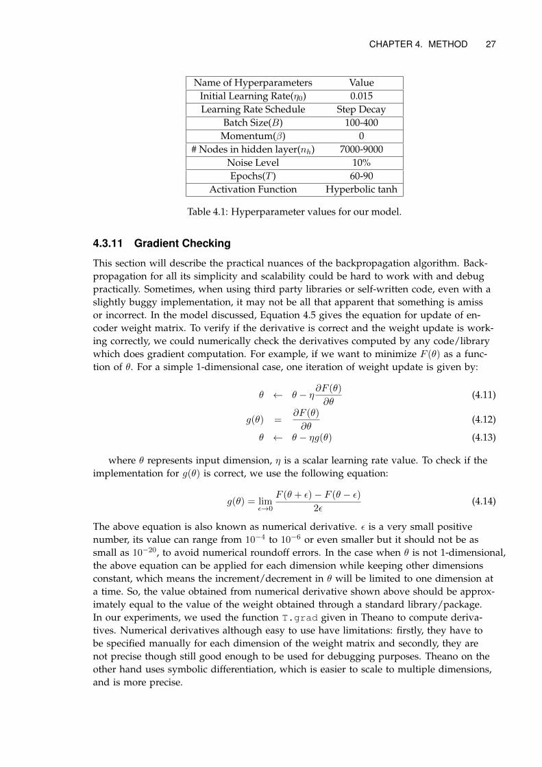
Name of Hyperparameters ValueInitial Learning Rate(η0) 0.015Learning Rate Schedule Step Decay
Batch Size(B) 100-400Momentum(β) 0
# Nodes in hidden layer(nh) 7000-9000Noise Level 10%Epochs(T ) 60-90
Activation Function Hyperbolic tanh
Table 4.1: Hyperparameter values for our model.
4.3.11 Gradient Checking
This section will describe the practical nuances of the backpropagation algorithm. Back-propagation for all its simplicity and scalability could be hard to work with and debugpractically. Sometimes, when using third party libraries or self-written code, even with aslightly buggy implementation, it may not be all that apparent that something is amissor incorrect. In the model discussed, Equation 4.5 gives the equation for update of en-coder weight matrix. To verify if the derivative is correct and the weight update is work-ing correctly, we could numerically check the derivatives computed by any code/librarywhich does gradient computation. For example, if we want to minimize F (θ) as a func-tion of θ. For a simple 1-dimensional case, one iteration of weight update is given by:
θ ← θ − η∂F (θ)
∂θ(4.11)
g(θ) =∂F (θ)
∂θ(4.12)
θ ← θ − ηg(θ) (4.13)
where θ represents input dimension, η is a scalar learning rate value. To check if theimplementation for g(θ) is correct, we use the following equation:
g(θ) = limε→0
F (θ + ε)− F (θ − ε)2ε
(4.14)
The above equation is also known as numerical derivative. ε is a very small positivenumber, its value can range from 10−4 to 10−6 or even smaller but it should not be assmall as 10−20, to avoid numerical roundoff errors. In the case when θ is not 1-dimensional,the above equation can be applied for each dimension while keeping other dimensionsconstant, which means the increment/decrement in θ will be limited to one dimension ata time. So, the value obtained from numerical derivative shown above should be approx-imately equal to the value of the weight obtained through a standard library/package.In our experiments, we used the function T.grad given in Theano to compute deriva-tives. Numerical derivatives although easy to use have limitations: firstly, they have tobe specified manually for each dimension of the weight matrix and secondly, they arenot precise though still good enough to be used for debugging purposes. Theano on theother hand uses symbolic differentiation, which is easier to scale to multiple dimensions,and is more precise.
Chapter 5
Experiment Setup and Results
The model described in Chapter 4 is tested on two different datasets and the results arecompared with a standard two layer neural network. The first dataset is MNIST [27],which is used as a benchmark among the machine learning community for testing semi-supervised algorithms. As this thesis concentrates on improving semi-supervised classifi-cation on ASR, we also test the algorithm on TIMIT [10], which is a much bigger datasetthan MNIST, and quite popular in speech recognition community due to its carefullymanual annotated transcriptions.
5.1 Data
5.1.1 MNIST
We test performance on the standard MNIST [27] digit classification benchmark. Thedataset contains 10 digits from 0 to 9 each having 5000 sample points in the trainingset, and 1000 sample points in validation and test sets. The datapoints for each digitclass represent intra-class variation in the form of different artistic strokes. All the im-ages in the dataset are of size 28*28, which amounts to 784 pixels. The dataset for semi-supervised learning is created by splitting the total 50000 training samples between a la-beled and unlabeled set, and varying the number of the labeled points from 100 to 3000.All digit classes have the same number of points in the training set to avoid any bias forany particular class. This way, we ensure that all classes are balanced and have equalrepresentation in the labeled part of dataset. The MNIST in total contains 70000 samples:50000 in training set, 10000 in validation set and 10000 in test set. Some images from thedataset are shown in Fig. 5.1 The image is vectorised by concatenating all the pixels row-wise. We do not do any pre-processing of the images, and all the pixels of the image rep-resented by the vector is fed as input to the network.
5.1.2 TIMIT
The main part of this thesis is the experiment on the standard TIMIT dataset [10] for thetask of frame-based phone classification. TIMIT has a total of 6300 American English sen-tences corresponding to about 5.4 hours of speech recording, with 630 unique individualspeakers each having spoken 10 sentences. The spoken sentences were carefully chosento be phonetically rich. The speech waveform sampled at 16KHz frequency and stored in
28
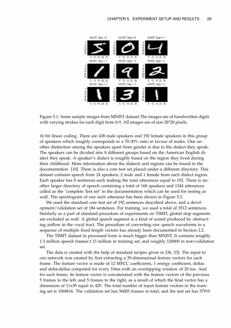
CHAPTER 5. EXPERIMENT SETUP AND RESULTS 29
Figure 5.1: Some sample images from MNIST dataset.The images are of handwritten digitswith varying strokes for each digit from 0-9. All images are of size 28*28 pixels.
16 bit linear coding. There are 438 male speakers and 192 female speakers in this groupof speakers which roughly corresponds to a 70-30% ratio in favour of males. One an-other distinction among the speakers apart from gender is due to the dialect they speak.The speakers can be divided into 8 different groups based on the American English di-alect they speak. A speaker’s dialect is roughly based on the region they lived duringtheir childhood. More information about the dialects and regions can be found in thedocumentation [10]. There is also a core test set placed under a different directory. Thisdataset contains speech from 24 speakers, 2 male and 1 female from each dialect region.Each speaker has 8 sentences each making the total utterances equal to 192. There is an-other larger directory of speech containing a total of 168 speakers and 1344 utterancescalled as the "complete Test set" in the documentation which can be used for testing aswell. The spectrogram of one such utterance has been shown in Figure 5.2.
We used the standard core test set of 192 sentences described above, and a devel-opment/validation set of 184 sentences. For training, we used a total of 3512 sentences.Similarly as a part of standard procedure of experiments on TIMIT, glottal stop segmentsare excluded as well. A glottal speech segment is a kind of sound produced by obstruct-ing airflow in the vocal tract. The procedure of converting raw speech waveforms to asequence of multiple fixed length vectors has already been documented in Section 2.2.
The TIMIT dataset in processed form is much bigger than MNIST, It contains roughly1.3 million speech frames:1.15 million in training set, and roughly 120000 in test+validationset.
The data is created with the help of standard recipes given in [36, 33]. The input toour network was created by first extracting a 39-dimensional feature vectors for eachframe. The feature vector is made of 12 MFCC coefficients, 1 energy coefficient, deltasand delta-deltas computed for every 10ms with an overlapping window of 20 ms. Andfor each frame, its feature vector is concatenated with the feature vectors of the previous5 frames to the left, and 5 frames to the right, as a result of which the final vector has adimension of 11x39 equal to 429. The total number of input feature vectors in the train-ing set is 1068816. The validation set has 56005 frames in total, and the test set has 57919
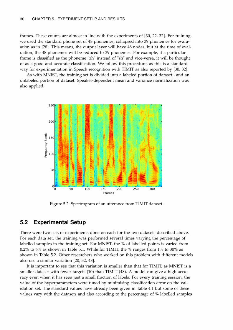
30 CHAPTER 5. EXPERIMENT SETUP AND RESULTS
frames. These counts are almost in line with the experiments of [30, 22, 32]. For training,we used the standard phone set of 48 phonemes, collapsed into 39 phonemes for evalu-ation as in [28]. This means, the output layer will have 48 nodes, but at the time of eval-uation, the 48 phonemes will be reduced to 39 phonemes. For example, if a particularframe is classified as the phoneme "zh" instead of "sh" and vice-versa, it will be thoughtof as a good and accurate classification. We follow this procedure, as this is a standardway for experimentation in Speech recognition with TIMIT as also reported by [30, 32].
As with MNIST, the training set is divided into a labeled portion of dataset , and anunlabeled portion of dataset. Speaker-dependent mean and variance normalization wasalso applied.
0 50 100 150 200 250 300Frames
0
50
100
150
200
250
Freq
uenc
y Ba
nds
Figure 5.2: Spectrogram of an utterance from TIMIT dataset.
5.2 Experimental Setup
There were two sets of experiments done on each for the two datasets described above.For each data set, the training was performed several times varying the percentage oflabelled samples in the training set. For MNIST, the % of labelled points is varied from0.2% to 6% as shown in Table 5.1. While for TIMIT, the % ranges from 1% to 30% asshown in Table 5.2. Other researchers who worked on this problem with different modelsalso use a similar variation [20, 32, 48].
It is important to see that this variation is smaller than that for TIMIT, as MNIST is asmaller dataset with fewer targets (10) than TIMIT (48). A model can give a high accu-racy even when it has seen just a small fraction of labels. For every training session, thevalue of the hyperparameters were tuned by minimising classification error on the val-idation set. The standard values have already been given in Table 4.1 but some of thesevalues vary with the datasets and also according to the percentage of % labelled samples
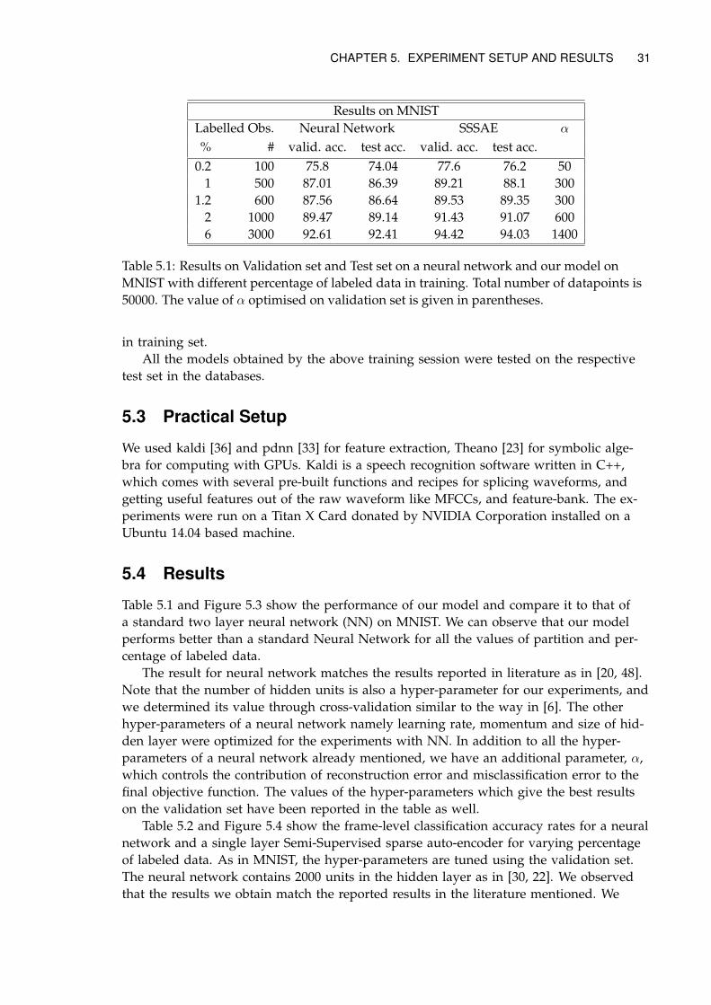
CHAPTER 5. EXPERIMENT SETUP AND RESULTS 31
Results on MNISTLabelled Obs. Neural Network SSSAE α
% # valid. acc. test acc. valid. acc. test acc.0.2 100 75.8 74.04 77.6 76.2 50
1 500 87.01 86.39 89.21 88.1 3001.2 600 87.56 86.64 89.53 89.35 300
2 1000 89.47 89.14 91.43 91.07 6006 3000 92.61 92.41 94.42 94.03 1400
Table 5.1: Results on Validation set and Test set on a neural network and our model onMNIST with different percentage of labeled data in training. Total number of datapoints is50000. The value of α optimised on validation set is given in parentheses.
in training set.All the models obtained by the above training session were tested on the respective
test set in the databases.
5.3 Practical Setup
We used kaldi [36] and pdnn [33] for feature extraction, Theano [23] for symbolic alge-bra for computing with GPUs. Kaldi is a speech recognition software written in C++,which comes with several pre-built functions and recipes for splicing waveforms, andgetting useful features out of the raw waveform like MFCCs, and feature-bank. The ex-periments were run on a Titan X Card donated by NVIDIA Corporation installed on aUbuntu 14.04 based machine.
5.4 Results
Table 5.1 and Figure 5.3 show the performance of our model and compare it to that ofa standard two layer neural network (NN) on MNIST. We can observe that our modelperforms better than a standard Neural Network for all the values of partition and per-centage of labeled data.
The result for neural network matches the results reported in literature as in [20, 48].Note that the number of hidden units is also a hyper-parameter for our experiments, andwe determined its value through cross-validation similar to the way in [6]. The otherhyper-parameters of a neural network namely learning rate, momentum and size of hid-den layer were optimized for the experiments with NN. In addition to all the hyper-parameters of a neural network already mentioned, we have an additional parameter, α,which controls the contribution of reconstruction error and misclassification error to thefinal objective function. The values of the hyper-parameters which give the best resultson the validation set have been reported in the table as well.
Table 5.2 and Figure 5.4 show the frame-level classification accuracy rates for a neuralnetwork and a single layer Semi-Supervised sparse auto-encoder for varying percentageof labeled data. As in MNIST, the hyper-parameters are tuned using the validation set.The neural network contains 2000 units in the hidden layer as in [30, 22]. We observedthat the results we obtain match the reported results in the literature mentioned. We
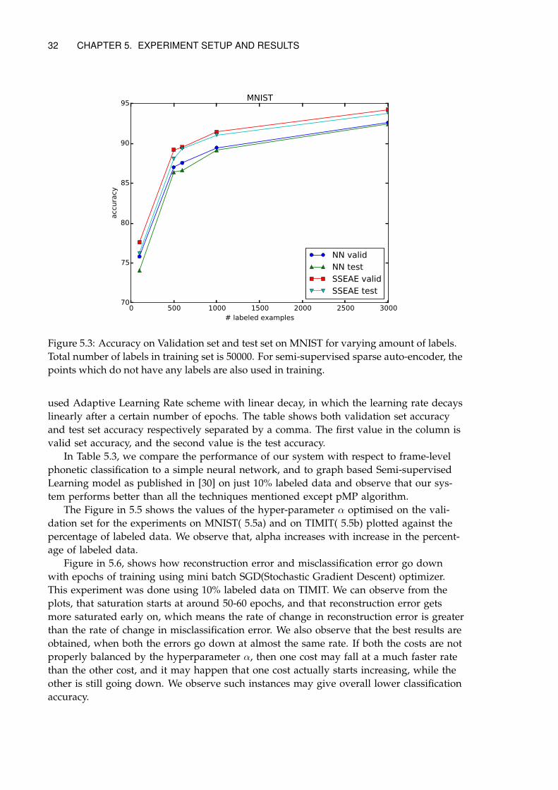
32 CHAPTER 5. EXPERIMENT SETUP AND RESULTS
0 500 1000 1500 2000 2500 3000# labeled examples
70
75
80
85
90
95ac
cura
cy
MNIST
NN validNN testSSEAE validSSEAE test
Figure 5.3: Accuracy on Validation set and test set on MNIST for varying amount of labels.Total number of labels in training set is 50000. For semi-supervised sparse auto-encoder, thepoints which do not have any labels are also used in training.
used Adaptive Learning Rate scheme with linear decay, in which the learning rate decayslinearly after a certain number of epochs. The table shows both validation set accuracyand test set accuracy respectively separated by a comma. The first value in the column isvalid set accuracy, and the second value is the test accuracy.
In Table 5.3, we compare the performance of our system with respect to frame-levelphonetic classification to a simple neural network, and to graph based Semi-supervisedLearning model as published in [30] on just 10% labeled data and observe that our sys-tem performs better than all the techniques mentioned except pMP algorithm.
The Figure in 5.5 shows the values of the hyper-parameter α optimised on the vali-dation set for the experiments on MNIST( 5.5a) and on TIMIT( 5.5b) plotted against thepercentage of labeled data. We observe that, alpha increases with increase in the percent-age of labeled data.
Figure in 5.6, shows how reconstruction error and misclassification error go downwith epochs of training using mini batch SGD(Stochastic Gradient Descent) optimizer.This experiment was done using 10% labeled data on TIMIT. We can observe from theplots, that saturation starts at around 50-60 epochs, and that reconstruction error getsmore saturated early on, which means the rate of change in reconstruction error is greaterthan the rate of change in misclassification error. We also observe that the best results areobtained, when both the errors go down at almost the same rate. If both the costs are notproperly balanced by the hyperparameter α, then one cost may fall at a much faster ratethan the other cost, and it may happen that one cost actually starts increasing, while theother is still going down. We observe such instances may give overall lower classificationaccuracy.
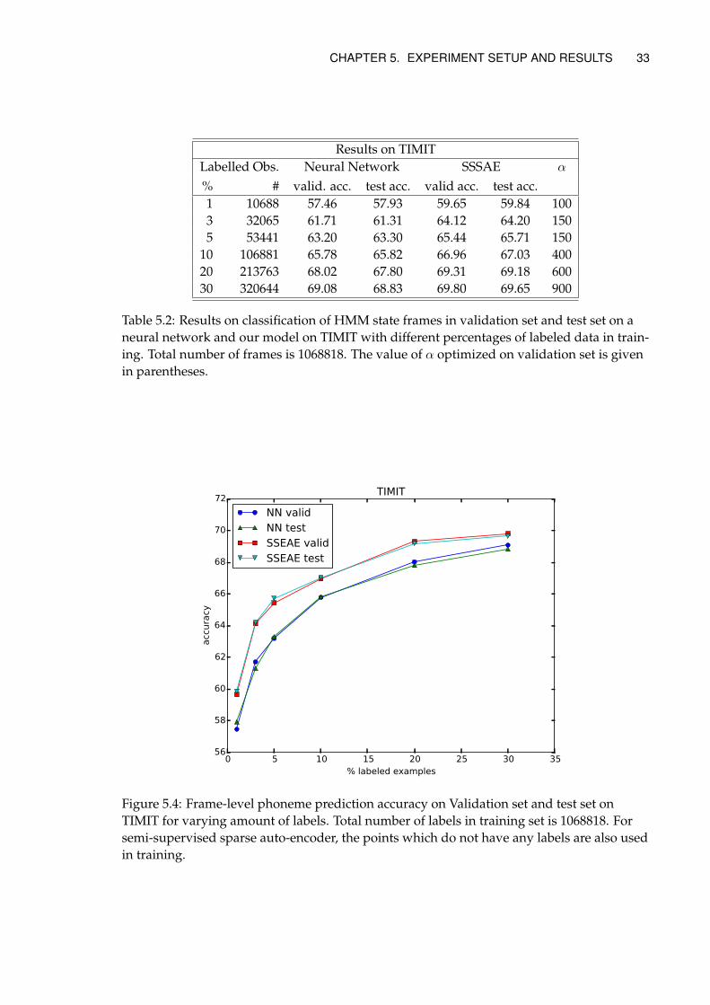
CHAPTER 5. EXPERIMENT SETUP AND RESULTS 33
Results on TIMITLabelled Obs. Neural Network SSSAE α
% # valid. acc. test acc. valid acc. test acc.1 10688 57.46 57.93 59.65 59.84 1003 32065 61.71 61.31 64.12 64.20 1505 53441 63.20 63.30 65.44 65.71 150
10 106881 65.78 65.82 66.96 67.03 40020 213763 68.02 67.80 69.31 69.18 60030 320644 69.08 68.83 69.80 69.65 900
Table 5.2: Results on classification of HMM state frames in validation set and test set on aneural network and our model on TIMIT with different percentages of labeled data in train-ing. Total number of frames is 1068818. The value of α optimized on validation set is givenin parentheses.
0 5 10 15 20 25 30 35% labeled examples
56
58
60
62
64
66
68
70
72
accu
racy
TIMIT
NN validNN testSSEAE validSSEAE test
Figure 5.4: Frame-level phoneme prediction accuracy on Validation set and test set onTIMIT for varying amount of labels. Total number of labels in training set is 1068818. Forsemi-supervised sparse auto-encoder, the points which do not have any labels are also usedin training.
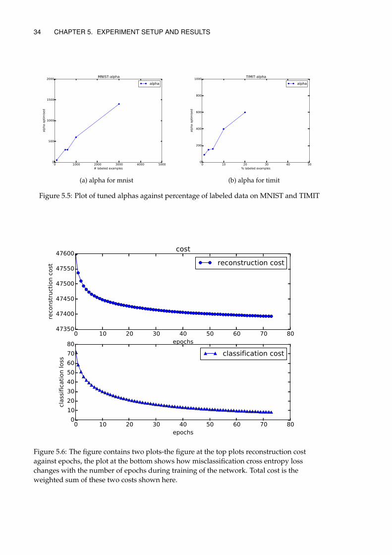
34 CHAPTER 5. EXPERIMENT SETUP AND RESULTS
0 1000 2000 3000 4000 5000# labeled examples
0
500
1000
1500
2000
alph
a op
timis
ed
MNIST-alpha
alpha
(a) alpha for mnist
0 10 20 30 40 50% labeled examples
0
200
400
600
800
1000
alph
a op
timis
ed
TIMIT-alpha
alpha
(b) alpha for timit
Figure 5.5: Plot of tuned alphas against percentage of labeled data on MNIST and TIMIT
0 10 20 30 40 50 60 70 80epochs
47350
47400
47450
47500
47550
47600
reco
nstr
uctio
n co
st
cost
reconstruction cost
0 10 20 30 40 50 60 70 80epochs
01020304050607080
clas
sific
atio
n lo
ss
classification cost
Figure 5.6: The figure contains two plots-the figure at the top plots reconstruction costagainst epochs, the plot at the bottom shows how misclassification cross entropy losschanges with the number of epochs during training of the network. Total cost is theweighted sum of these two costs shown here.
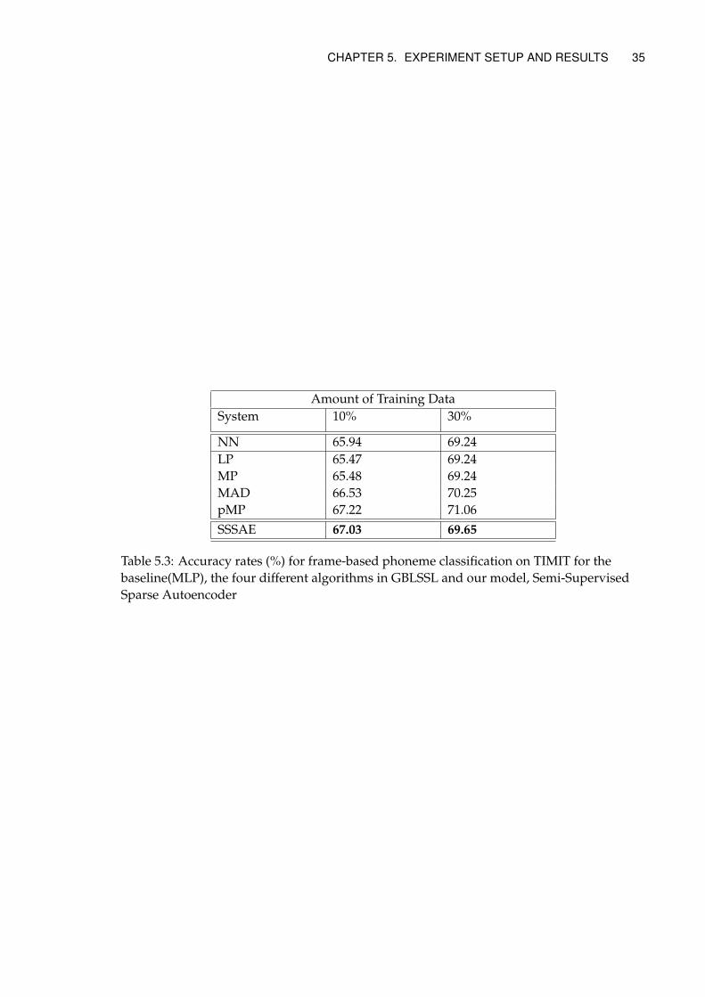
CHAPTER 5. EXPERIMENT SETUP AND RESULTS 35
Amount of Training DataSystem 10% 30%
NN 65.94 69.24LP 65.47 69.24MP 65.48 69.24MAD 66.53 70.25pMP 67.22 71.06SSSAE 67.03 69.65
Table 5.3: Accuracy rates (%) for frame-based phoneme classification on TIMIT for thebaseline(MLP), the four different algorithms in GBLSSL and our model, Semi-SupervisedSparse Autoencoder
Chapter 6
Discussion, Conclusion and Future Work
This report is concluded by a discussion on the performance of the algorithm and theevaluation methods proposed.
6.1 Hypotheses discussed
6.1.1 H.1 Do Semi-Supervised Sparse Autoencoders perform better than neu-ral networks on phone classification?
The results from our experiments validate the ability of autoencoders to use unlabeleddata to find the manifold of the data distribution, which can be effectively used to boostaccuracy on labeled data classification in speech domain for the task of frame-level phonemeclassification.
6.1.2 H.2 Does the above result generalize to other domains?
We have observed a similar improvement in classification accuracy of written digits onthe MNIST dataset. This suggests that the improvements obtained by this model may beextended to a variety of tasks. It can be observed that this improvement is present whenthe percentage of labeled data is varied from 0.2% to 6% .
6.1.3 H.3: Do Semi-Supervised Sparse Autoencoders perform better than GBLSSL methods on phoneme classification?
In this case, the results we obtain are similar to those found in the literature in similarconditions. We can conclude that our method obtains similar results with smaller compu-tational requirements. In order to quantify the difference, however we should perform adetailed complexity analysis of both approaches.
We notice that autoencoders are easy to be modelled, and conceptually easy to be ex-plained. We also observed that we did not need to use any particular initialisation forthe network and pretraining as sometimes required in learning of autoencoders. This isan improvement on a standard auto-encoder which can be explored more in future work.
36
CHAPTER 6. DISCUSSION, CONCLUSION AND FUTURE WORK 37
6.2 Evaluation Method
The evaluation method for the purpose of this thesis was classification accuracy. We per-formed experiments on two different datasets. For MNIST, the criterion was better clas-sification on the test set. For TIMIT, the criterion was better classification accuracy ofphonemes for all the individual speech frames in the test set. Regarding the choice ofthe percentage of labeled data at which the experiments were performed, we can arguethat in nature in general, we always find an abundance of unlabeled data, so it becomesmore important for us to investigate our models when the percentage of labeled data isvery low. Also, as the percentage of labeled datapoints increase, the accuracy starts tosaturate, and any subsequent increase in percentage of labeled examples does not bringin much of improvement in the accuracy as observed in the lower percentages of data.This seems reasonable, as after a certain percentage of data, the model knows the inputdistribution almost completely, and only small improvements in knowledge are observedhenceforth. The size of the labeled points for our experiments is varied from 1% to 30%of the entire training set frames count.
Finally, it is also important to note that most standard and industry-grade speech pro-cessing systems need to handle units like phones, words that are inherently of variablelength. In other-words, improvement in accuracy of frame-level based phoneme classi-fication might be a good indicator, but it cannot be definitely said, that overall speechrecognition accuracy when measured in terms of word-recognition will definitely in-crease. Though, most researchers in the community still focus on frame-level phonemeaccuracy as the first goal, before moving on to the harder challenge of word recognitionand recognition of variable-length "large" speech segments like sentences.
6.3 Effect of α in the model
It can be observed from Figure 5.5, that the value of alpha increases as the proportionof labeled data in the training set is varied. The factor α plays an important role in bal-ancing out the two different kind of costs involved. The two costs are orthogonal andserve different purposes. The classification cost is discriminative in nature, but it can notbe the only objective cost as that will lead to severe overfitting, the reconstruction costacts as a regulariser and makes the network determine the structure or distribution ofthe data. One possible explanation for the monotonic increase, is that the network has al-ready seen enough of unlabeled data to decipher its structure so that it starts optimisingon the classification cost to get a better classification accuracy on the validation set. Weused cross-validation to tune the value of α for each experiment. Generally, the plot oferror on validation set with α is a U-shaped curve. This means that, the accuracy startsincreasing and becomes maximum at a certain value of α and then starts dropping again.
6.4 Future Work
There are many exciting ideas and research directions in which this work could be ex-tended. Firstly, we could use feature-bank features described in Section 2.2 on featureprocessing from raw waveform. Though MFCCs and their deltas have been effective asfeatures for phoneme recognition, they are highly compressed. Using feature banks in-stead might give a higher accuracy. One objective of using MFCCs was to compare with
38 CHAPTER 6. DISCUSSION, CONCLUSION AND FUTURE WORK
the results of [30] who also have used MFCCs for GBL Semi-Supervised Learning. Asdiscussed above, a logical next step would be to apply the algorithm for segment classifi-cation task. That way, it could be definitely said that, the algorithm is good for speechprocessing and recognition applications. One more research direction could be to useeven more advanced and powerful auto-encoders like Variational Autoencoders or Gen-erative Adversarial Autoencoders on speech data in semisupervised setting.
6.5 Society and Ethics
Speech Recognition in the past decade has reached to the end user in the form of hear-ing aids, and through the popularisation of dialogue systems like Apple Siri, Alexa byAmaxon, Cortana by Microsoft. The potential effect of research on these models is to im-prove quality of life especially for people with disabilities. Speech technology-based aidsare often non available for minority languages. For those languages the limited commer-cial interest does not justify the investment required to collect expensive hand-annotatedspeech material that is necessary to train speech recognition models. The purpose of thisthesis is to improve the existing techniques in Speech Recognition so that the need forexpensive annotated recordings is reduced. This would make speech technology avail-able to all citizens regardless if they speak a popular language or a more remote one.
During this thesis we used standardised data sets with speech recordings from Amer-ican English speakers. All the ethical values were considered in this recordings, includinganonymity, gender balance, dialectal balance.

Chapter 7
Appendix
Phoneme MappingPhoneme-48 Phoneme-39aa aaae aeah ahao aaaw awax ahay ayb bch chcl sild ddh dhdx dxeh ehel len nepi siler erey eyf fg ghh hhih ihix ih
Phoneme MappingPhoneme-48 Phoneme-39iy iyjh jhk kl lm mn nng ngow owoy oyp pr rs ssh shsil silt tth thuh uhuw uwv vvcl silw wy yz zzh sh
Table 7.1: Mapping between 48 phonemes used for training and 39 phonemes used forevaluation
39
Bibliography
[1] Ossama Abdel-Hamid, Abdel-Rahman Mohamed, Hui Jiang, Li Deng, Gerald Penn,and Dong Yu. Convolutional neural networks for speech recognition. IEEE/ACMTrans. Audio, Speech and Lang. Proc., 22(10):1533–1545, October 2014.
[2] Andrei Alexandrescu and Katrin Kirchhoff. Graph-based learning for phonetic clas-sification. In IEEE Workshop on Automatic Speech Recognition & Understanding, ASRU2007, Kyoto, Japan, December 9-13, 2007, pages 359–364, 2007.
[3] Y. Bengio, P. Lamblin, D. Popovici, and H. Larochelle. Greedy layer-wise training ofdeep networks. In B. Schölkopf, J. Platt, and T. Hoffman, editors, Advances in NeuralInformation Processing Systems 19, pages 153–160. MIT Press, Cambridge, MA, 2007.
[4] Yoshua Bengio. Practical recommendations for gradient-based training of deep archi-tectures. In Neural Networks: Tricks of the Trade - Second Edition, pages 437–478. 2012.
[5] Léon Bottou. Stochastic gradient descent tricks. In Neural Networks: Tricks of the Trade- Second Edition, pages 421–436. 2012.
[6] A. Coates, H. Lee, and A.Y. Ng. An analysis of single-layer networks in unsuper-vised feature learning. In Geoffrey Gordon, David Dunson, and Miroslav Dudík,editors, Proceedings of the Fourteenth International Conference on Artificial Intelligenceand Statistics, volume 15 of JMLR Workshop and Conference Proceedings, pages 215–223.JMLR W&CP, 2011.
[7] G. E. Dahl, D. Yu, L. Deng, and A. Acero. Context-dependent pre-trained deep neu-ral networks for large-vocabulary speech recognition. IEEE Transactions on Audio,Speech, and Language Processing, 20(1):30–42, Jan 2012.
[8] Steven Davis and Paul Mermelstein. Improvements to filterbank and delta learningwithin a deep neural network framework. In IEEE Transactions on Acoustics, Speech,and Signal Processing, volume 28. IEEE, 1980.
[9] Li Deng Alex Acero Dong Yu, Balakrishnan Varadarajan. Active learning and semi-supervised learning for speech recognition: A unified framework using the globalentropy reduction maximization criterion. Elsevier, January 2009.
[10] William M. Fisher, George R. Doddington, and Kathleen M. Goudie-Marshall. Thedarpa speech recognition research database: Specifications and status. In Proceedingsof DARPA Workshop on Speech Recognition, pages 93–99, 1986.
[11] M.J.F. Gales. Maximum likelihood linear transformations for hmm-based speechrecognition. Computer Speech and Language, 12:75–98, 1998.
40
BIBLIOGRAPHY 41
[12] Xavier Glorot and Yoshua Bengio. Understanding the difficulty of training deepfeedforward neural networks. In Proceedings of the Thirteenth International Conferenceon Artificial Intelligence and Statistics, AISTATS 2010, Chia Laguna Resort, Sardinia, Italy,May 13-15, 2010, pages 249–256, 2010.
[13] Yves Grandvalet and Yoshua Bengio. Semi-supervised learning by entropy min-imization. In François Denis, editor, Actes de CAP 05, Conférence francophone surl’apprentissage automatique - 2005, Nice, France, du 31 mai au 3 juin 2005, pages 281–296.PUG, 2005.
[14] Alex Graves, Abdel rahman Mohamed, and Geoffrey E. Hinton. Speech recognitionwith deep recurrent neural networks. In ICASSP, pages 6645–6649. IEEE, 2013.
[15] Frantisek Grézl and Martin Karafiát. Semi-supervised bootstrapping approach forneural network feature extractor training. In 2013 IEEE Workshop on Automatic SpeechRecognition and Understanding, Olomouc, Czech Republic, December 8-12, 2013, pages470–475, 2013.
[16] Jui-Ting Huang and Mark Hasegawa-Johnson. Semi-supervised training of gaussianmixture models by conditional entropy minimization. In Takao Kobayashi, KeikichiHirose, and Satoshi Nakamura, editors, INTERSPEECH 2010, 11th Annual Conferenceof the International Speech Communication Association, Makuhari, Chiba, Japan, September26-30, 2010, pages 1353–1356. ISCA, 2010.
[17] Yan Huang, Dong Yu, Yifan Gong, and Chaojun Liu. Semi-supervised GMM andDNN acoustic model training with multi-system combination and confidence re-calibration. In INTERSPEECH 2013, 14th Annual Conference of the International SpeechCommunication Association, Lyon, France, August 25-29, 2013, pages 2360–2364, 2013.
[18] Thorsten Joachims. Transductive inference for text classification using support vectormachines. In Ivan Bratko and Saso Dzeroski, editors, Proceedings of ICML-99, 16thInternational Conference on Machine Learning, pages 200–209, Bled, SL, 1999. MorganKaufmann Publishers, San Francisco, US.
[19] Kelley Kilanski, Jonathan Malkin, Xiao Li, Richard Wright, and Jeff A. Bilmes. Thevocal joystick data collection effort and vowel corpus. In INTERSPEECH 2006 - IC-SLP, Ninth International Conference on Spoken Language Processing, Pittsburgh, PA, USA,September 17-21, 2006, 2006.
[20] Diederik P. Kingma, Danilo Jimenez Rezende, Shakir Mohamed, and Max Welling.Semi-supervised learning with deep generative models. CoRR, abs/1406.5298, 2014.
[21] Alex Krizhevsky, Ilya Sutskever, and Geoffrey E. Hinton. Imagenet classificationwith deep convolutional neural networks. In F. Pereira, C. J. C. Burges, L. Bottou,and K. Q. Weinberger, editors, Advances in Neural Information Processing Systems 25,pages 1097–1105. Curran Associates, Inc., 2012.
[22] John Labiak and Karen Livescu. Nearest neighbors with learned distances for pho-netic frame classification. In Interspeech, 2011.
42 BIBLIOGRAPHY
[23] Pascal Lamblin, Razvan Pascanu, James Bergstra, Ian J. Goodfellow, Arnaud Berg-eron, Nicolas Bouchard, and Yoshua Bengio. Theano: new features and speed im-provements. 2012.
[24] Lori Lamel, Jean-Luc Gauvain, and Gilles Adda. Investigating lightly supervisedacoustic model training. In IEEE International Conference on Acoustics, Speech, and Sig-nal Processing, ICASSP 2001, 7-11 May, 2001, Salt Palace Convention Center, Salt Lake City,Utah, USA, Proceedings, pages 477–480. IEEE, 2001.
[25] Lori Lamel, Jean-Luc Gauvain, and Gilles Adda. Lightly supervised and unsuper-vised acoustic model training. Computer Speech & Language, 16(1):115–129, 2002.
[26] T. Landauer, C. Kamm, and S. Singhal. Learning a minimally structured back propa-gation network to recognize speech. In 9th Annu. Conf. Cogn. Sci. Soc., pages 531–536,1987.
[27] Yann LeCun and Corinna Cortes. MNIST handwritten digit database.http://yann.lecun.com/exdb/mnist/, 2010.
[28] K. F. Lee and H. W. Hon. Speaker-independent phone recognition using hid-den markov models. IEEE Transactions on Acoustics, Speech, and Signal Processing,37(11):1641–1648, Nov 1989.
[29] C. J. Leggetter and P. C. Woodland. Maximum likelihood linear regression forspeaker adaptation of continuous density hidden Markov models. Computer Speechand Language, pages 171–185, 1995.
[30] Yuzong Liu and Katrin Kirchhoff. Graph-based semi-supervised learning forphone and segment classification. In Frédéric Bimbot, Christophe Cerisara, CécileFougeron, Guillaume Gravier, Lori Lamel, François Pellegrino, and Pascal Perrier,editors, INTERSPEECH, pages 1840–1843. ISCA, 2013.
[31] Yuzong Liu and Katrin Kirchhoff. Graph-based semi-supervised acoustic modelingin DNN-based speech recognition. In Proceedings of the IEEE Spoken Language Technol-ogy Workshop (SLT), pages 177–182, 2014.
[32] Yuzong Liu and Katrin Kirchhoff. Graph-based semisupervised learning for acousticmodeling in automatic speech recognition. IEEE/ACM Trans. Audio, Speech & LanguageProcessing, 24(11):1946–1956, 2016.
[33] Y. Miao. Kaldi+PDNN: Building DNN-based ASR Systems with Kaldi and PDNN.ArXiv e-prints, January 2014.
[34] Vinod Nair and Geoffrey E. Hinton. Rectified linear units improve restricted boltz-mann machines. In Johannes Fürnkranz and Thorsten Joachims, editors, ICML,pages 807–814. Omnipress, 2010.
[35] Andrew Ng. Stanford university lecture notes on sparse autoencoders. 2011.
[36] Daniel Povey, Arnab Ghoshal, Gilles Boulianne, and Burget. The kaldi speech recog-nition toolkit. In IEEE 2011 Workshop on Automatic Speech Recognition and Understand-ing. IEEE Signal Processing Society, December 2011. IEEE Catalog No.: CFP11SRW-USB.
BIBLIOGRAPHY 43
[37] Daniel Povey, Dimitri Kanevsky, Brian Kingsbury, Bhuvana Ramabhadran, GeorgeSaon, and Karthik Visweswariah. Boosted mmi for model and feature-space discrim-inative training. In ICASSP, pages 4057–4060. IEEE, 2008.
[38] Abdel rahman Mohamed, Tara N. Sainath, George E. Dahl, Bhuvana Ramabhadran,Geoffrey E. Hinton, and Michael A. Picheny. Deep belief networks using discrimina-tive features for phone recognition. In ICASSP, pages 5060–5063. IEEE, 2011.
[39] Marc’Aurelio Ranzato and Martin Szummer. Semi-supervised learning of compactdocument representations with deep networks. In William W. Cohen, Andrew Mc-Callum, and Sam T. Roweis, editors, ICML, volume 307 of ACM International Confer-ence Proceeding Series, pages 792–799. ACM, 2008.
[40] Chuck Rosenberg, Martial Hebert, and Henry Schneiderman. Semi-supervised self-training of object detection models. In WACV/MOTION, pages 29–36. IEEE Com-puter Society, 2005.
[41] Tara Sainath, Brian Kingsbury, Abdel-Rahman Mohamed, and Bhuvana Ramabhad-ran. Learning filter banks within a deep neural network framework. In IEEE Interna-tional Conference on Acoustic, Speech and Signal Processing. IEEE, 2014.
[42] George Saon, Hong-Kwang Jeff Kuo, Steven J. Rennie, and Michael Picheny. TheIBM 2015 english conversational telephone speech recognition system. CoRR,abs/1505.05899, 2015.
[43] Frank Seide, Gang Li, Xie Chen, and Dong Yu. Feature engineering in context-dependent deep neural networks for conversational speech transcription. In 2011IEEE Workshop on Automatic Speech Recognition & Understanding, ASRU 2011, Waikoloa,HI, USA, December 11-15, 2011, pages 24–29, 2011.
[44] Amarnag Subramanya, Jeff Bilmes, and Yoshua Bengio. Semi-supervised learningwith measure propagation. Journal of Machine Learning. Research, pages 3311–3370,2011.
[45] Partha Pratim Talukdar and Koby Crammer. New regularized algorithms for trans-ductive learning. In Wray L. Buntine, Marko Grobelnik, Dunja Mladenic, and JohnShawe-Taylor, editors, ECML/PKDD (2), volume 5782 of Lecture Notes in Computer Sci-ence, pages 442–457. Springer, 2009.
[46] Karel Veselý, Mirko Hannemann, and Lukáš Burget. Semi-supervised training ofdeep neural networks. In Proceedings of IEEE Conference on Automatic Speech Recogni-tion and Understanding (ASRU), pages 267–272, 2013.
[47] Frank Wessel and Hermann Ney. Unsupervised training of acoustic models for largevocabulary continuous speech recognition. IEEE Trans. Speech and Audio Processing,13(1):23–31, 2005.
[48] Jason Weston, Frédéric Ratle, Hossein Mobahi, and Ronan Collobert. Deep learn-ing via semi-supervised embedding. In Grégoire Montavon, Genevieve B. Orr, andKlaus-Robert Müller, editors, Neural Networks: Tricks of the Trade (2nd ed.), volume 7700of Lecture Notes in Computer Science, pages 639–655. Springer, 2012.

44 BIBLIOGRAPHY
[49] Xiaojin Zhu and Zoubin Ghahramani. Learning from labeled and unlabeled datawith label propagation. Technical report, 2002.
[50] Xiaojin Zhu, Jaz S. Kandola, Zoubin Ghahramani, and John D. Lafferty. Nonpara-metric transforms of graph kernels for semi-supervised learning. In NIPS, pages1641–1648, 2004.

www.kth.se