Citation: Samee, N.A.; Atteia, G.;

Alkanhel, R.; Alhussan, A.A.; AlEisa,

H.N. Hybrid Feature Reduction

Using PCC-Stacked Autoencoders for

Gold/Oil Prices Forecasting under

COVID-19 Pandemic. Electronics

2022, 11, 991. https://doi.org/

10.3390/electronics11070991

Academic Editor: Grzegorz Dudek

Received: 15 February 2022

Accepted: 17 March 2022

Published: 23 March 2022

Publisher’s Note: MDPI stays neutral

with regard to jurisdictional claims in

published maps and institutional affil-

iations.

Copyright: © 2022 by the authors.

Licensee MDPI, Basel, Switzerland.

This article is an open access article

distributed under the terms and

conditions of the Creative Commons

Attribution (CC BY) license (https://

creativecommons.org/licenses/by/

4.0/).

electronics

Article

Hybrid Feature Reduction Using PCC-Stacked Autoencodersfor Gold/Oil Prices Forecasting under COVID-19 PandemicNagwan Abdel Samee 1 , Ghada Atteia 1 , Reem Alkanhel 1,* , Amel Ali Alhussan 2

and Hussah Nasser AlEisa 2

1 Department of Information Technology, College of Computer and Information Sciences,Princess Nourah bint Abdulrahman University, P.O. Box 84428, Riyadh 11671, Saudi Arabia;nmabdelsamee@pnu.edu.sa (N.A.S.); geatteiaallah@pnu.edu.sa (G.A.)

2 Department of Computer Sciences, College of Computer and Information Sciences,Princess Nourah bint Abdulrahman University, P.O. Box 84428, Riyadh 11671, Saudi Arabia;aaalhussan@pnu.edu.sa (A.A.A.); haleisa@pnu.edu.as (H.N.A.)

* Correspondence: rialkanhal@pnu.edu.sa; Tel.: +966-55-050-6818

Abstract: The financial markets have been influenced by the emerging spread of Coronavirus disease,COVID-19. The oil, and gold as well have experienced a downward trend due to the increased rate inthe number of confirmed COVID-19 cases. Lately, the published COVID data comprised new variablesthat may influence the accuracy of the oil/gold prices forecasting models including the Stringencyindex, Reproduction rate, Positive Rate, and Vaccinations. In this study, Deep Autoencoders areintroduced and combined with the well-known approach: Pearson Correlation Coefficient, PCC,analysis in selecting the key features that affect the accuracy of the forecasting models of gold andoil prices with respect to COVID-19 pandemic. We have utilized a hybrid approach of PCC alongwith a 2-Stage Stacked Autoencoder, SA, to extract the latent features which are then submitted toNeural Network, NN, regression model. The NN regressor has been trained using the BayesianRegularization-backpropagation algorithm which provides a good generalization for small noisydatasets. The hybrid approach has yielded the minimum MSE values of 8.97× 10−3 and 5.356 × 10−2

on the oil/gold validation set, respectively. Compared to the existing approaches, the proposedapproach has outperformed the ARIMA, ML based regression models in forecasting the oil/goldprices. In addition, the introduced framework has yielded lower Mean Absolute Error, MAE, thanthe Recurrent Neural Network, RNN, and the Principal Component Analysis, PCA, for dimensionreduction. The retrieved results showed that the hybrid method produced more robust features byconsidering the relationship between the input features.

Keywords: stacked autoencoders; neural network; forecasting models

1. Introduction

Forecasting the prices of gold and oil has a great impact on the market participants,and portfolio risk management. Oil and gold are two important commodities for theglobal economy that are frequently included in equities portfolios of investors [1]. Highuncertainty about the oil and gold prices may reduce the investments and increase investorworries, making portfolio risk management and asset allocation a big challenge for equityinvestors, traders, hedgers, and portfolio managers [2]. Oil prices are highly volatile, andthe price fluctuations are a good predictor for forecasting commodities and financial assetprices. On the other hand, gold is often seen as a safe-haven asset during times of crisis [3].Stockholders frequently switch between or bring together, oil and gold to vary their equityportfolios [4]. Lately, both commodities have been indicated by increasing instability andthis has confused the investment decision-making. Therefore, accurate forecasting of the oiland gold prices may help the investors in taking their portfolio risk management decisions.

Electronics 2022, 11, 991. https://doi.org/10.3390/electronics11070991 https://www.mdpi.com/journal/electronics

Electronics 2022, 11, 991 2 of 23

Once the COVID-19 pandemic occurred in China, the virus has been spread all overthe world and it has significantly increased the uncertainty in the prices of the commoditymarkets including gold and oil [5]. The growth in the rate of mortality has forced thegovernments to enforce harsh restrictions including lockdowns and hold many businessoperations which have had serious consequences for economies and financial sectors [6].As most of the economic activities have been halted during the lockdowns in approximatelyall industrialized economies, the price of the crude oil fell during 2020 and while the goldprices have taken an upward trend [7,8].

The existing methods for the forecasting of the oil and gold prices can be divided intotwo categories including spatial-based or historical-based prediction models [9]. Froma spatial point of view, the forecasting model is constructed based on the factors thatinfluence oil/gold prices. However, in the historical perspective, the construction is basedon the historical values of the prices. Basically, the oil/gold prices have direct interactionsamong other market factors including the stock prices, and the US dollar [10]. As wellas during the COVID-19 pandemic, the indirect impact of commodity markets has alsoaffected the oil/gold prices. Therefore, spatial-based forecasting for oil/gold prices is theproper method during the COVID-19 pandemic.

Although the forecasting of the oil and gold prices during the Covid-19 pandemic isemerging, still few studies have been published in the literature in this regard. Mensi et al. [5]have investigated the price-switching spillovers between the stock, gold, and crude oil,futures prices before and during the global health crisis, COVID-19 pandemic. The para-metric autoregressive technique has been employed to detect the connectedness betweenthe stock, oil, and gold prices during the COVID-19. Dimitrios Bakas et al. [7] have empiri-cally estimated the three 5-factor Vector Auto-Regressive, VAR, model for the instability ofcommodity markets including crude oil, broad commodity index, and gold.

Originally, there are various ML algorithms have been utilized for the forecastingof gold and crude oil prices. Such publications include classical ML regressors suchas the ANN, SVM, and GPR [9,11–15] and Deep Learning algorithms [16–21]. Lately,ANNs have yielded outstanding performance in describing the nonlinear relationshipsamong variables [22]. Moshiri and Foroutan [12] have set up a nonlinear ANN model forforecasting the crude oil prices from 1983 to 2003. The retrieved results using the ANN havesurpassed the results yielded from the ARIMA, and GARCH regressors. Wang et al. [20]have utilized the filter and wrapper feature selection approaches to improve the retrievedperformance of the ANN, and the SVM. Kristjanpoller and Minutolo [14] have proposeda hybrid frame including the ANN and GARCH in the prediction of crude oil and thecomposite model has yielded a better performance compared to the stand-alone ones.The overfitting of the ANN in forecasting the financial data has been resolved in [23]by introducing the Bayesian Regularization approach as a training algorithm. The deeplearning-based forecasting models are based on time series analysis for the historical valuesof the gold and crude oil prices. The recurrent neural network, RNN, and the Long-termand Short-term Memory Model, LSTM, are deep learning approaches that consider thejoint relationship of the long-term and short-term factors of crude oil, and gold prices [9].

The accuracy of the forecasting data model is greatly impacted by the significanceof the input features [24]. Selecting the significant input features is accomplished usingfilter or wrapper methods. The PCC analysis is the dominant filter-based feature selectionmethod for building forecasting models [25]. In the PCC analysis, the correlation coefficientbetween the outcome and input features is computed. Significant input features are thosethat are highly correlated with the response variable. Although the correlation-basedfeature selection is an early approach in building a forecasting data model, it does notensure the dependency between the outcome and the selected input predictors. Instead, themulti-layer deep learning models such as Autoencoder [23] lately have yielded outstandingperformance in extracting the latent deep features in the feature matrix [26].

In this study, we are introducing a hybrid approach including Deep Autoencoders,and Pearson correlation analysis in selecting the key features that affect the accuracy of

Electronics 2022, 11, 991 3 of 23

Crude oil and gold forecasting models during the COVID-19 pandemic. The retrievedsignificant features are used in the training and validation of an NN regressor which haslately yielded an outstanding performance in the forecasting of such commodities.

This research article paper is constructed as follows: a literature review is introducedin Section 2. The methods including the data exploration and its preprocessing, andthe proposed PCC-Stacked Autoencoders model are explained in Section 3. Results aredisplayed and examined in Section 4. Lastly, the conclusion of the presented study isdescribed in Section 5.

2. Literature Review

The data models for the prediction of gold and oil prices can be divided into twocategories: empirical, and regression-based methods [27]. The main principle in theEconometrics models in estimating the prices based on the theories that estimate the in-teraction of buyers and sellers. The Random Walk Hypothesis, RWH, and the EfficientMarket Hypothesis, EMH, are the leading theoretical models that describe such interac-tions [28]. Although the empirical models for identifying gold, and crude oil prices areefficient for accurate prediction, they are in some way complicated. Therefore, regressionmethods are utilized to deal with ambiguous relationships between various factors. Inthe regression-based methods, the parametric and non-parametric regression can be uti-lized [29]. Lately, the Autoregressive Integrated Moving Average, ARIMA, and GeneralizedAutoregressive Conditional Heteroskedasticity, GARCH, models have been utilized [11,12].The parametric regression is efficient if there is Gaussian distribution for the values ofthe outcomes [30]. Otherwise, the nonparametric ones are more efficient [31]. Usually,the parametric methods are more powerful than nonparametric for datasets containinga small number of samples [32]. The regression-based model includes autoregression,and artificial intelligence-based methods. The Markov-switching vector is an example forautoregression, while the Artificial intelligence forecasting models include the artificialneural network (ANN) [33], Gaussian process regression (GPR) [34], and support vectormachine (SVM) [35].

The oil/gold prices forecasting is challenging due to its nonlinear characteristics.Therefore, the research in this field never ends. For example, Yu et al. [36] have built ahistorical-based forecasting model for the oil prices during the period (1990–2008). Theyhave used the SVM regressor and compared the performance to the ARIMA regressors.SVM has surpassed the ARIMA, but they cannot describe the nonlinear relationship of oilprices and ignore the relations of short-term influences. Another historical-based predictionis carried out in [37] using the classical ML regression techniques and the retrieved resultswere compared with the well-known regressor, ARIMA. The nonlinear characteristics ofthe oil/gold prices have been handled by utilizing the ANN regression models such as thework carried out by [12]. They have also built a historical-based regression model usingthe ANN approach and compared their performance with the linear methods including theARIMA and GARCH methods during the period (1983 to 2003). Indranil et al. [38] haveutilized the ANN, and LSTM [39] in enhancing an existing stochastic model for analyzingthe commodity market, Barndorff-Nielsen, and Shephard model. The utilization of MLapproaches in that stochastic model has handled its weak points such as the absence oflong-term dependence between influencing factors.

The impact of input features being used in the training of the oil/gold forecastingmodels has been studied in few studies such as the work carried out in [20]. They haveintroduced filter, wrapper, and hybrid feature selection methods to detect the significantfactors that may influence the accuracy of the prediction of the oil price. Linear regression,ANN, and SVM have been utilized in the training of forecasting models. The utilization offeature selection in that study facilitated the achievement of the outstanding performancefor the forecasting models. The dimension reduction of the feature space has been intro-duced in [9] in forecasting the oil prices. The PCA along with locally linear embeddingand the multidimensional scale as dimensional reduction techniques have been used and

Electronics 2022, 11, 991 4 of 23

compared. RNN, and LSTM as historical-based forecasting models have been employed inbuilding the forecasting models.

The common conclusion among the aforementioned studies is that the forecastingof the crude oil and gold prices during the COVID-19 is demanding advanced forecast-ing models to overcome the nonlinearity of its characteristics. The promising resultsyielded using the ANN generally along with the increased accuracy observed using deeplearning methods encourage this study to accomplish better accuracy using the featureextraction methodologies.

This study contributes the following:

• Analysis of recently published COVID-19 data sets along with the crude oil, and goldprices during that global health crisis and studying the impact of high spread andmortality rates, precautionary measures, and vaccinations on the prices ofsuch commodities.

• Deep Autoencoders are integrated with the correlation analysis approach in selectingthe key features that affect the accuracy of the forecasting models.

• The Bayesian regularization-backpropagation algorithm is utilized to avoid the over-fitting of data which is a major drawback of training ANNs on the small-size datasets.

3. Methods

In this study, we have followed the framework depicted in Figure 1. The data set hasbeen integrated from four public data sets including the COVID-19 records published bythe Johns Hopkins University Center for Systems Science and Engineering web site [40],the World Daily Spot Prices for Crude Oil WTI, and Brent [41] published by King AbdullahPetroleum Studies and Research Center, the World Gold Council [42], and the indexes ofthe stock market directions from Yahoo Finance [43]. Five stock markets indexes havebeen utilized in this study including Vanguard Total Stock Market (VUN), Vanguard TotalStock Market Index Fund ETF Shares (VTI), Vanguard Value Index Fund ETF Shares (VTV),Emerging Markets Index (MME), and the Emerging Markets NTR Index (MMN). Theintegrated dataset has been preprocessed to impute the missing values and normalization.Then the data records have been divided randomly into training/testing samples with apercentage of 70/30%, respectively. The training samples are utilized to build the predictionmodels while the testing samples are employed to evaluate their prediction accuracy. Thetraining/testing samples are then fed to a feature selection stage to select the key factorsthat may influence the prediction accuracy. We have conducted three different experimentsto decide the optimum approach. In the first experiments, the relevant features havebeen extracted using the PCC are fed to neural networks regressor. The relevant featuresextracted using the correlation analysis are the ones that have higher Pearson CorrelationCoefficient [44], with the outcomes. In the second experiment, the input variables arepassed to a 2-stages stacked autoencoder deep network to extract a set of distinguishinglatent features. The latent feature set is then fed to the regression model. Finally, in the thirdexperiment, we have combined the PCC analysis with deep autoencoders. The relevantfeatures extracted using the correlation analysis have been fed to the deep autoencoder toextract the latent features which are then submitted to the regression model. The fitting NNregressor that mapped the numeric input features to the numeric targets is two layers offeedforward NN with 10 sigmoid hidden neurons and linear transfer function in its outputneurons. The NN has been trained using the Bayesian Regularization-backpropagationalgorithm which can result in yielding a good generalization for small noisy datasets.

Electronics 2022, 11, 991 5 of 23

Figure 1. The framework of the proposed forecasting system for Gold, and Crude Oil prices.

Electronics 2022, 11, 991 6 of 23

3.1. Data Exploration and Hypothesis Testing3.1.1. Data Exploration and Preprocessing

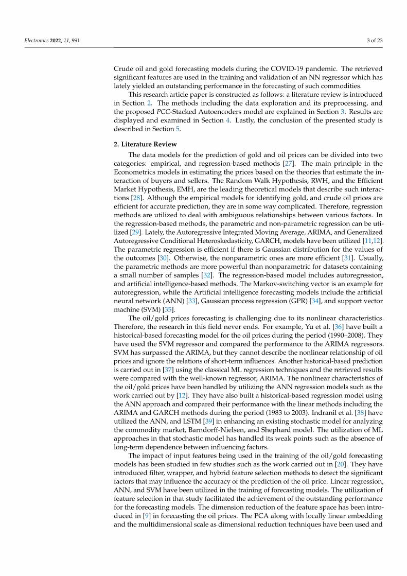
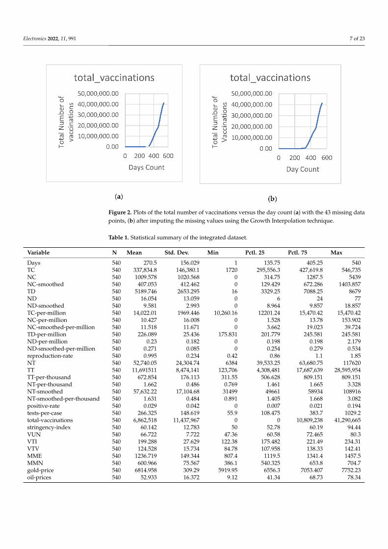
The COVID-19 data set records for Saudi Arabia have been downloaded starting from1 April 2020 to the end of September 2021, along with the corresponding prices for crudeoil, and gold in the same period. The Gold and oil datasets have several missing valuesbecause of market closures for weekends, and holidays. Therefore, the data values werepadded to interpolate the values of the missing entries. The padding is preferred overother interpolation approaches as it is more insightful to refer to the final exchange ratesand values as the current one. Additionally, there were two missing entries for the oilprices on 31 May 2021, and 30 August 2021, and they have been estimated by averagingthe adjacent values. The COVID data contains 36 variables including the number of newconfirmed cases, the total number of confirmed cases, new deaths, the total number ofdeaths, the total number of tests, and other supplementary entries. Lately, the publishedCOVID data contained new variables that may influence the accuracy of the forecastingmodels including the Stringency index, reproduction rate, Positive Rate, and vaccinations.Stringency index is a composite measure of the precautionary measures based on variousresponse indicators such as workplace closures, school closures, and travel bans. Thevalues of the Stringency index range from 0 to 100, the value of 100 denotes the strictestpolicies. The reproduction rate of coronavirus gives an estimate of the possible extent ofthe virus transmission. The Positive Rate is an indicator of the Spread of the Virus. Basedon the criteria announced by WHO in 2020, if the positive rate is less than 5% then thepandemic is under control in a country. The vaccination has been started in Saudi Arabiaon 7 January 2021, therefore all previous values before this date have been set to zero. Therewere 43 missing values in the vaccinations field that have been imputed using the GrowthInterpolation as depicted in Figure 2. The overall records in the data set are 540. Table 1depicts a statistical description of the integrated dataset. The entries of Table 1 provide asummary of the distribution of the data values including the count represented by symbolN, the mean, standard deviation, the minimum, the 1st quantile, the mean, the 2nd quantile,and the maximum. The distribution of varying variables is illustrated by the aid of drawingthe corresponding histogram as shown in Figure 3. The correlation matrix between allvariables except those having zero variance is illustrated in Figure 4. The oils prices showa higher correlation with the variables describing the COVID-19 spread and the marketprices than those for the gold prices.

Plots of the response variables versus the 540 days are shown in Figure 5. To preparethe integrated data records for the analysis, the entries have been normalized using thez-score approach. The normalized values are centralized around zero and have a standarddeviation of one. For a random variable X having a mean value of µ and a standarddeviation σ, the values of its z-scores are defined by Equation (1).

z-score =X− µ

σ(1)

There are several performance metrics to determine the loss in regression modelsincluding the Mean Square Error, MSE, and the R squared. All these metrics try to calculatethe differences between the forecasted, and the actual values as depicted in Equation (2)where N, yi, and yi are the number of observations, the actual, and the predicted values,respectively.

MSE =1N ∑N

i=1(yi − yi)2 (2)

Electronics 2022, 11, 991 7 of 23

Figure 2. Plots of the total number of vaccinations versus the day count (a) with the 43 missing datapoints, (b) after imputing the missing values using the Growth Interpolation technique.

Table 1. Statistical summary of the integrated dataset.

Variable N Mean Std. Dev. Min Pctl. 25 Pctl. 75 Max

Days 540 270.5 156.029 1 135.75 405.25 540TC 540 337,834.8 146,380.1 1720 295,556.3 427,619.8 546,735NC 540 1009.578 1020.568 0 314.75 1287.5 5439NC-smoothed 540 407.053 412.462 0 129.429 672.286 1403.857TD 540 5189.746 2653.295 16 3329.25 7088.25 8679ND 540 16.054 13.059 0 6 24 77ND-smoothed 540 9.581 2.993 0 8.964 9.857 18.857TC-per-million 540 14,022.01 1969.446 10,260.16 12201.24 15,470.42 15,470.42NC-per-million 540 10.427 16.008 0 1.528 13.78 153.902NC-smoothed-per-million 540 11.518 11.671 0 3.662 19.023 39.724TD-per-million 540 226.089 25.436 175.831 201.779 245.581 245.581ND-per-million 540 0.23 0.182 0 0.198 0.198 2.179ND-smoothed-per-million 540 0.271 0.085 0 0.254 0.279 0.534reproduction-rate 540 0.995 0.234 0.42 0.86 1.1 1.85NT 540 52,740.05 24,304.74 6384 39,533.25 63,680.75 117620TT 540 11,691511 8,474,141 123,706 4,308,481 17,687,639 28,595,954TT-per-thousand 540 672.854 176.113 311.55 506.628 809.151 809.151NT-per-thousand 540 1.662 0.486 0.769 1.461 1.665 3.328NT-smoothed 540 57,632.22 17,104.68 31499 49661 58934 108916NT-smoothed-per-thousand 540 1.631 0.484 0.891 1.405 1.668 3.082positive-rate 540 0.029 0.042 0 0.007 0.021 0.194tests-per-case 540 266.325 148.619 55.9 108.475 383.7 1029.2total-vaccinations 540 6,862,518 11,437,967 0 0 10,809,238 41,290,665stringency-index 540 60.142 12.783 50 52.78 60.19 94.44VUN 540 66.722 7.722 47.36 60.58 72.465 80.3VTI 540 199.288 27.629 122.38 175.482 221.49 234.31VTV 540 124.528 15.734 84.78 107.958 138.33 142.41MME 540 1236.719 149.344 807.4 1119.5 1341.4 1457.5MMN 540 600.966 75.567 386.1 540.325 653.8 704.7gold-price 540 6814.958 309.29 5919.95 6556.3 7053.407 7752.23oil-prices 540 52.933 16.372 9.12 41.34 68.73 78.34

Electronics 2022, 11, 991 8 of 23

Figure 3. Cont.

Electronics 2022, 11, 991 9 of 23

Figure 3. Cont.

Electronics 2022, 11, 991 10 of 23

Figure 3. Histograms of varying variables in the integrated dataset.

Electronics 2022, 11, 991 11 of 23

Figure 4. The correlation matrix of the integrated dataset (TC, NC, TD, ND, NT, and TT denotes TotalCases, New Cases, Total Deaths, New Deaths, New Tests, and Total Tests).

Figure 5. Plots of the Gold/Oil prices versus 540 Days under the COVID-19 Pandemic; (a) Goldprices; (b) Oil prices.

3.1.2. Hypothesis Testing

To assess the validity of the proposed models in making good predictions for the pricesof the oil, and gold prices during the COVID-19 pandemic, we have utilized the hypothesistesting for the whole population. In multiple linear regression, the null hypothesis ina population p can be formulated as H0 : β1 = 0, β2 = 0, β3 = 0, . . . βp = 0 whichreveals that there is no relationship between the outcome and the p input predictors.The model is effective if there any β 6= 0 which is called the alternative hypothesis Hawhere Ha : at least one β j 6= 0 (j = 1, . . . p). In this study, we have used the ANOVAF-statistics test as a way of hypothesis testing. We have excluded the variable that has zerovariance from the test. In regression-based problems, the test is performed by measuringthe significance level of the estimated coefficients yielded from linear regression models.The significance of each estimated coefficient is measured by calculating four metricsincluding the sum of squares (SS), the mean sum of squares (MS), the F-statistic, and thep-value. Table 2 displays the retrieved results of the test for the oil/gold prices. Basedon the retrieved values of both the F-value, and the p-value, the null hypothesis must berejected and it is revealed that there is a linear association between the outcomes (oil, andgold prices) and more than one of the input predictors in the integrated dataset.

Electronics 2022, 11, 991 12 of 23

Table 2. ANOVA test for the oil/gold prices and the input predictors.

Variable SymbolOil Prices Gold Prices

SS MSE F Value p-Value SS MSE F Value p-ValueTC 97.27 97.27 19.27 1.45 × 10−5 27,824,836 27,824,836 1511 1.91 × 10−138

NC 2879.85 2879.85 570.56 3.37 × 10−79 211,353.5 211,353.5 11.48 0.0007NC_smoothed 996.57 996.57 197.44 8.81 × 10−37 129,593.1 129,593.1 7.039 0.008

TD 90.75 90.75 17.98 2.77 × 10−5 6075.404 6075.404 0.33 0.565ND 22.07 22.07 4.37 0.037 93.30752 93.30752 0.005 0.943

ND_smoothed 1229.91 1229.91 243.67 2.66 × 10−43 230,428.2 230,428.2 12.51 0.0004TC_per_million 1370.09 1370.09 271.44 5.38 × 10−47 4677.894 4677.894 0.25 0.614NC_per_million 0.54 0.54 0.11 0.743 542.2688 542.2688 0.029 0.863

NC_smoothed_per_million 32.67 32.67 6.47 0.011 7617.666 7617.666 0.41 0.520TD_per_million 474.52 474.52 94.01 4.045 × 10−20 150,517.9 150,517.9 8.17 0.004ND_per_million 23.41 23.41 4.64 0.031 5520.553 5520.553 0.29 0.584

ND_smoothed_per_million 0.03 0.03 0.01 0.940 33,612.67 33,612.67 1.82 0.177reproduction_rate 440.53 440.53 87.28 6.51 × 10−19 149,960.9 149,960.9 8.146 0.004

NT 110.80 110.80 21.95 3.82 × 10−6 686,444.9 686,444.9 37.29 2.397TT 664.40 664.40 131.63 1.46 × 10−26 6409.206 6409.206 0.34 0.555

TT_per_thousand 15.63 15.63 3.10 0.079 266,227.8 266,227.8 14.46 0.0001NT_per_thousand 0.48 0.48 0.09 0.758 50,317.62 50,317.62 2.73 0.099

NT_smoothed 26.45 26.45 5.24 0.022 68,690.21 68,690.21 3.73 0.054NT_smoothed_per_thousand 1.19 1.19 0.24 0.627 38,354.85 38,354.85 2.08 0.149

positive_rate 85.52 85.52 16.94 4.671 × 10−5 10,960.87 10,960.87 0.59 0.44tests_per_case 6.72 6.72 1.33 0.249 130,501 130,501 7.089 0.008

total_vaccinations 556.24 556.24 110.20 5.95 × 10−23 1,404,073 1,404,073 76.27 6.66 × 10−17

stringency_index 3.56 3.56 0.71 0.40 631,517.1 631,517.1 34.3 9.78 × 10−9

VUN 4.68 4.68 0.93 0.33 4290.694 4290.694 0.23 0.629VTI 9.56 9.56 1.89 0.169 1,256,655 1,256,655 68.26 2.08 × 10−15

VTV 36.61 36.61 7.25 0.007 51,795.74 51,795.74 2.81 0.094MME 31.10 31.10 6.16 0.013 1038.809 1038.809 0.05 0.81MMN 19.89 19.89 3.94 0.0477 53,050.65 53,050.65 2.88 0.09

Gold_price 65.14 65.14 12.90 0.0003 237,554.9 237,554.9 12.9 0.0003

Electronics 2022, 11, 991 13 of 23

3.2. Pearson Correlation Coefficient Analysis

The Pearson Correlation Coefficient is an early method that finds the linear correlationbetween two random variables. PCC is a measure of similarity or dependency betweentwo vectors. The PCC can be calculated for a pair of vectors X, and Y using Equation (3).Equation (4) represents the estimation for the PCC. If the input variables, X, and Y arecorrelated, the value of the PCC is between −1, and +1, linearly dependent. Otherwise, it iszero if they are uncorrelated.

PCC =cov(X, Y)

2√

σ(X)σ(Y)(3)

PCC =E(XY)− E(X)E(Y)

2√

σ(X)σ(Y)(4)

where, E() is the expectation operator, σ(X), and σ(Y) are the variances of the variable X,and Y correspondingly, and cov(X, Y) is the covariance matrix between them.

3.3. Stacked Deep Autoencoder

Autoencoder is a deep neural network used to learn a compressed representation ofinput data [22]. The autoencoder is trained to ignore insignificant data, noise, and its outputis an encoding version for a set of data. This is the main idea in using the autoencoderfor dimensional reduction of the feature space. The autoencoder comprises two modulesincluding an encoder followed by a decoder [22]. The encoder module maps the inputvariables to a compressed form while the decoder tries to reverse the mapping to regeneratethe input [22]. In this study, sparse autoencoders have been trained in an unsupervisedmanner using the Scaled Conjugate Gradient Algorithm, SCGA, [24] with 1000 trainingepochs. The autoencoder is used to extract the latent features and ignore the irrelevantones. The input variables have been fed to the autoencoder and the number of neuronsin the hidden layer has been adjusted to be less than the size of the input. We combinedsparsity in the autoencoders by adding up a regularizer for the neurons’ activations tothe cost function [23]. As depicted in Equation (5), the cost function is the mean squarederror function adjusted to contain two terms: the weight regularization, Ω_weights, andthe sparsity regularization, Ω_sparsity [45]. The sparsity regularizer restricts the outputfrom a neuron to be low allowing the autoencoder to discover a representation from asmall portion of the training samples [23]. The weight regularization term avoids thevalues of the neuron weights from increasing which subsequently could reduce the sparsityregularizer. Equations (6) and (7) illustrate the mathematical representations of Ω_weights,and Ω_sparsity, respectively.

E =1M

M

∑n=1

N

∑k=1

(xkn − xkn)2

︸ ︷︷ ︸mean squared error

+λ×Ωweights+β×Ωsparsity

(5)

In Equation (3), M is a number of samples in the training subset, N is the number ofinput variables in the training data, x is a training sample, x is the estimate of the trainingsample, β, and λ are the coefficients of the sparsity, and weight regularizer, respectively [41].

Ωweights =1M

L

∑l

M

∑j

K

∑i

(w(l)

ji

)2(6)

Electronics 2022, 11, 991 14 of 23

In Equation (4), L represents the size of hidden layers, w is the weight matrix [41].

Ωsparsity =D(1)

∑i=1

KL (ρ‖ρi)

=D(1)

∑i=1

ρ log(

ρρi

)+(1− ρ) log

(1−ρ1−ρi

) (7)

f (z) =

0, i f z ≤ 0z, i f 0 < z < 11, i f z ≥ 1

(8)

In Equation (5), ρi denotes the average activation of neuron i, while ρ represent thedesired activation and, KL denotes the Kullback-Leibler divergence value between ρi andρ [41].

As depicted in Figure 6, we have utilized a stacked autoencoders, 2 stages, beginningby training the first autoencoder, Autoencoder 1, on the input variables and using theextracted features from Autoencoder 1 as input to the second stage, Autoencoder 2. Thetransfer function used for the first encoder (Encoder 1) is the positive saturating lineartransfer while the ordinary linear transfer function is used for the first decoder (Decoder1). Positive saturating linear has been utilized in the encoder, and the decoder modulesas depicted in Equation (8). We have set the learning parameters as shown in Table 3. Inour experiment, all input variables: M = 36, N = 540 have been fed to Autoencoder 1.The number of extracted features from stage 1 was 10 features so the number of inputs toAutoencoder 2 have been as follows M = 10, N = 540. We have extracted 5 significant fea-tures from Autoencoder 2 and used them in the prediction phase. However, in experimentc, we have used the relevant features extracted by the correlation analysis, 22 features, asinputs to autoencoder 1. We have conducted many trials to set the values of all the learningparameters and the recorded values here are the ones that have yielded the minimum rootmean squared error for the predicted values of the response variables.

Figure 6. Two- Stages stacked deep autoencoder for Selecting Key features for Forecasting the oil,and gold prices.

Electronics 2022, 11, 991 15 of 23

Table 3. The values for the learning parameters used in the training of Autoencoder 1, and Autoen-coder 2 in the stacked deep autoencoder.

Learning Parameters Values

ρ (Sparsity Proportion) 0.05

β (Sparsity Regularization) 4

λ (coefficient of the weight regularizer) 0.002

No. of Epochs 1000

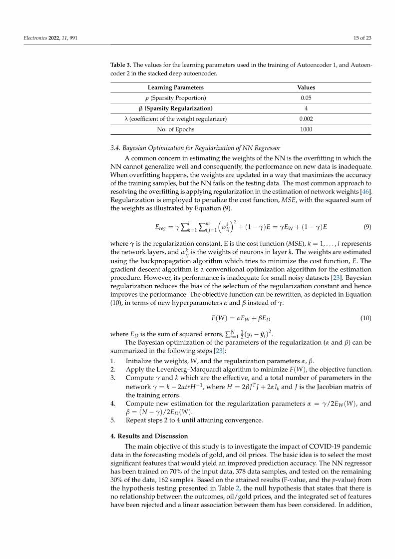
3.4. Bayesian Optimization for Regularization of NN Regressor

A common concern in estimating the weights of the NN is the overfitting in which theNN cannot generalize well and consequently, the performance on new data is inadequate.When overfitting happens, the weights are updated in a way that maximizes the accuracyof the training samples, but the NN fails on the testing data. The most common approach toresolving the overfitting is applying regularization in the estimation of network weights [46].Regularization is employed to penalize the cost function, MSE, with the squared sum ofthe weights as illustrated by Equation (9).

Ereg = γ ∑lk=1 ∑m

i,j=1

(wk

ij

)2+ (1− γ)E = γEW + (1− γ)E (9)

where γ is the regularization constant, E is the cost function (MSE), k = 1, . . . , l representsthe network layers, and wk

ij is the weights of neurons in layer k. The weights are estimatedusing the backpropagation algorithm which tries to minimize the cost function, E. Thegradient descent algorithm is a conventional optimization algorithm for the estimationprocedure. However, its performance is inadequate for small noisy datasets [23]. Bayesianregularization reduces the bias of the selection of the regularization constant and henceimproves the performance. The objective function can be rewritten, as depicted in Equation(10), in terms of new hyperparameters α and β instead of γ.

F(W) = αEW + βED (10)

where ED is the sum of squared errors, ∑Ni=1

12 (yi − yi)

2.The Bayesian optimization of the parameters of the regularization (α and β) can be

summarized in the following steps [23]:

1. Initialize the weights, W, and the regularization parameters α, β.2. Apply the Levenberg–Marquardt algorithm to minimize F(W), the objective function.3. Compute γ and k which are the effective, and a total number of parameters in the

network γ = k− 2αtrH−1, where H = 2βJT J + 2αIk and J is the Jacobian matrix ofthe training errors.

4. Compute new estimation for the regularization parameters α = γ/2EW(W), andβ = (N − γ)/2ED(W).

5. Repeat steps 2 to 4 until attaining convergence.

4. Results and Discussion

The main objective of this study is to investigate the impact of COVID-19 pandemicdata in the forecasting models of gold, and oil prices. The basic idea is to select the mostsignificant features that would yield an improved prediction accuracy. The NN regressorhas been trained on 70% of the input data, 378 data samples, and tested on the remaining30% of the data, 162 samples. Based on the attained results (F-value, and the p-value) fromthe hypothesis testing presented in Table 2, the null hypothesis that states that there isno relationship between the outcomes, oil/gold prices, and the integrated set of featureshave been rejected and a linear association between them has been considered. In addition,

Electronics 2022, 11, 991 16 of 23

the nonlinearity in such interactions can be detected via the deep autoencoder and theBayesian-based NN regression model.

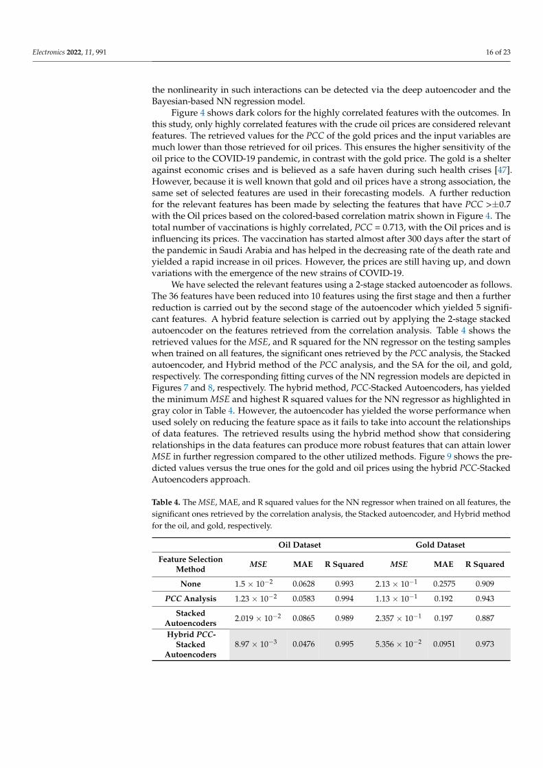
Figure 4 shows dark colors for the highly correlated features with the outcomes. Inthis study, only highly correlated features with the crude oil prices are considered relevantfeatures. The retrieved values for the PCC of the gold prices and the input variables aremuch lower than those retrieved for oil prices. This ensures the higher sensitivity of theoil price to the COVID-19 pandemic, in contrast with the gold price. The gold is a shelteragainst economic crises and is believed as a safe haven during such health crises [47].However, because it is well known that gold and oil prices have a strong association, thesame set of selected features are used in their forecasting models. A further reductionfor the relevant features has been made by selecting the features that have PCC >±0.7with the Oil prices based on the colored-based correlation matrix shown in Figure 4. Thetotal number of vaccinations is highly correlated, PCC = 0.713, with the Oil prices and isinfluencing its prices. The vaccination has started almost after 300 days after the start ofthe pandemic in Saudi Arabia and has helped in the decreasing rate of the death rate andyielded a rapid increase in oil prices. However, the prices are still having up, and downvariations with the emergence of the new strains of COVID-19.

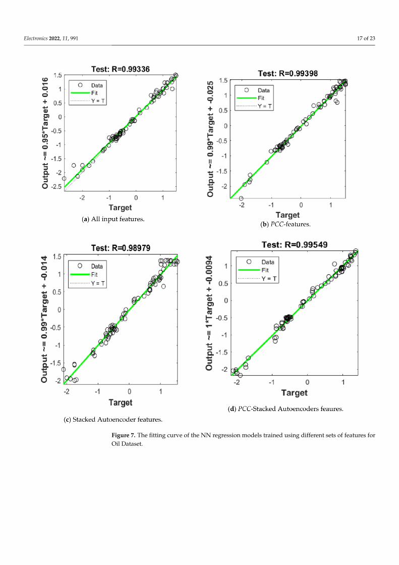
We have selected the relevant features using a 2-stage stacked autoencoder as follows.The 36 features have been reduced into 10 features using the first stage and then a furtherreduction is carried out by the second stage of the autoencoder which yielded 5 signifi-cant features. A hybrid feature selection is carried out by applying the 2-stage stackedautoencoder on the features retrieved from the correlation analysis. Table 4 shows theretrieved values for the MSE, and R squared for the NN regressor on the testing sampleswhen trained on all features, the significant ones retrieved by the PCC analysis, the Stackedautoencoder, and Hybrid method of the PCC analysis, and the SA for the oil, and gold,respectively. The corresponding fitting curves of the NN regression models are depicted inFigures 7 and 8, respectively. The hybrid method, PCC-Stacked Autoencoders, has yieldedthe minimum MSE and highest R squared values for the NN regressor as highlighted ingray color in Table 4. However, the autoencoder has yielded the worse performance whenused solely on reducing the feature space as it fails to take into account the relationshipsof data features. The retrieved results using the hybrid method show that consideringrelationships in the data features can produce more robust features that can attain lowerMSE in further regression compared to the other utilized methods. Figure 9 shows the pre-dicted values versus the true ones for the gold and oil prices using the hybrid PCC-StackedAutoencoders approach.

Table 4. The MSE, MAE, and R squared values for the NN regressor when trained on all features, thesignificant ones retrieved by the correlation analysis, the Stacked autoencoder, and Hybrid methodfor the oil, and gold, respectively.

Oil Dataset Gold Dataset

Feature SelectionMethod MSE MAE R Squared MSE MAE R Squared

None 1.5 × 10−2 0.0628 0.993 2.13 × 10−1 0.2575 0.909

PCC Analysis 1.23 × 10−2 0.0583 0.994 1.13 × 10−1 0.192 0.943

StackedAutoencoders 2.019 × 10−2 0.0865 0.989 2.357 × 10−1 0.197 0.887

Hybrid PCC-Stacked

Autoencoders8.97 × 10−3 0.0476 0.995 5.356 × 10−2 0.0951 0.973

Electronics 2022, 11, 991 17 of 23

Figure 7. The fitting curve of the NN regression models trained using different sets of features forOil Dataset.

Electronics 2022, 11, 991 18 of 23

Figure 8. The fitting curves of the NN regression models trained using different sets of features forGold Dataset.

Electronics 2022, 11, 991 19 of 23

Figure 9. The predicted values versus the true ones for the gold and oil prices versus 540 daysduring the COVID-19 pandemic using the hybrid feature extraction-based approach and NNregression models.

The performance of the proposed framework is evaluated versus several state-of-the-art forecasting models for oil, and gold prices. We compared our framework to thatdeveloped by Yu et al. [37], Xin James [48], Yan et al. [9], Weng et al. [49], He et al. [50],Khani et al. [51], and Jabeur et al. [52] as depicted in Table 5. The comparison shows thatthe proposed framework achieves the minimum RMSE, MSE, and MAE for forecasting theoil prices overall mentioned studies. The results yielded in this study have outperformedthe early regression method, ARIMA, and the classical ML regressors including the SVR,and ANN. High performance has been attained by the help of using the proposed featureselection mechanism. In addition, we have compared our approach to another work [9] thathas employed the feature reduction on the feature space of predicting the oil prices. Theyhave retrieved 0.0844 for the MAE which is higher than the corresponding value yieldedin our approach, 0.0476. Regarding the retrieved results for forecasting the gold prices,it has surpassed the ones yielded by the Multivariate Empirical Mode Decompositionapproach [50] and is comparable with the attained results by Khani et al. [51]. The study ofYan et al. [9] in particular, was picked for comparison as it is very close to our proposedframework so far. Both studies similarly have utilized feature reduction approaches forselecting the significant features for building the forecasting models. However, Yan’sstudy was applied only on oil datasets and used different methods rather than the deepautoencoder for the reduction of the feature space including the principal componentanalysis, PCA, locally linear embedding, LLE, and multidimensional scale, MDS.

Electronics 2022, 11, 991 20 of 23

Table 5. Comparing the results of the proposed framework for forecasting the oil, and gold prices with state-of the-art forecasting models.

Publication Method Dataset MSE R Squared MAE RMSE

Yu et al. [37] Support Vector Regression (SVR), ANN, and ARIMA Crude Oil - - -5.0493(ARIMA)

3.9337(SVR)4.8682(ANN)

Xin James [48] SVR, and ARIMA Crude Oil prices - - 1.1433(ARIMA)1.1246(SVR) -

Yan et al. [9] De-dimension machine learning model using PCA,and RNN/LSTM approach to forecast the oil prices. Crude Oil prices - -

0.0844(RNN)0.0905 (LSTM)0.2784 (SVM)

-

Weng et al. [49] Gold prices prediction using GA-ROSELM, genetic algorithmregularization online extreme learning machine

silver price, oil price,gold price - - 5.681 -

He et al. [50] Denoising model to detect the noise factors in forecasting metalprice using Multivariate Empirical Mode Decomposition Silver, and gold prices 1.222 - - 1.105

Khani et al. [51] Encoder–decoder LSTM model for forecasting gold pricesduring the COVID-19 pandemic.

COVID-19 data records,and gold prices 0.0217 0.858 - 0.147

Jabeur et al. [52] XGBoost machine learning approach for forecasting gold prices. Metals, oil, andgold prices - 0.994 21.948 -

Proposed framework PCC-Stacked Autoencoder Hybrid feature extraction approach forforecasting the oil, and gold prices during the COVID-19 pandemic.

COVID-19 data records,oil, and gold prices

0.0089 (oil)0.0536 (gold)

0.995 (oil)0.973 (gold)

0.0476 (oil)0.0951 (gold)

0.094 (oil)0.231 (gold)

Electronics 2022, 11, 991 21 of 23

5. Conclusions

The global lockdown carried out with respect to the COVID-19 pandemic has severeconsequences on the economy of the whole world. Oil and gold as well as experienced adownward trend due to the increased rate in the number of confirmed COVID-19 cases.Therefore, accurate forecasting for the oil, and gold during the COVID-19 period may assistthe investors and stakeholders in their risk management decisions.

This study is the first one to investigate the impact of the lately published featuresof COVID-19 datasets that may influence the accuracy of the oil/gold prices forecastingmodels including the Stringency index, reproduction rate, Positive Rate, and Vaccina-tions. Based on the PCC analysis, the total number of vaccinations is positively correlated,PCC = 0.713, with the Oil prices and is strongly influencing its prices. The vaccination hasaided in a rapid increase in oil prices. However, the developments of the new strains ofCOVID-19 are causing the instability of its prices. The yielded results provide an indicationthat the gold prices are more stable and have less sensitivity compared to the oil. The goldtends to respond in contrast with the other kinds of commodities which are highly affectedwith respect to the COVID-19 pandemic.

Deep autoencoders along with a Bayesian NN regressor are adopted to investigatethe impact of COVID-19 pandemic datasets on gold/oil prices during the period 1 April2020–30 September 2021 in Saudi Arabia. The key factors in the feature space that mayinfluence the accuracy of the forecasting models are selected using a hybrid approach ofstacked autoencoders and the Pearson Correlation analysis. The applied feature reductionmethods including PCC, 2-stage Stacked Autoencoder, and the PCC-Stacked Autoencodersdemonstrate that the hybrid approach has yielded more significant features by consideringthe relationship between the input features using the PCC. These key features have attainedthe minimum MSE, and highest R squared values for the NN regressor compared to othermethods. The presented approach for forecasting the oil/gold prices has outperformed theearly well-known regression technique, ARIMA, the classical ML (SVR, and ANN), anddeep learning methods (RNN, and LSTM).

Author Contributions: Conceptualization, N.A.S. and G.A.; methodology, N.A.S., G.A., R.A., A.A.A.and H.N.A.; software, N.A.S. and G.A.; validation, N.A.S. and G.A.; formal analysis, N.A.S., G.A.,R.A., A.A.A. and H.N.A.; investigation, N.A.S., G.A., R.A., A.A.A. and H.N.A.; resources, N.A.S.; datacuration, N.A.S.; writing—original draft preparation, N.A.S., G.A., R.A., A.A.A. and H.N.A.; writing—review and editing, N.A.S., G.A., R.A., A.A.A. and H.N.A.; visualization, N.A.S.; supervision, H.N.A.;project administration, R.A.; funding acquisition, R.A. All authors have read and agreed to thepublished version of the manuscript.

Funding: This research was funded by Princess Nourah bint Abdulrahman University ResearchersSupporting Project number (PNURSP2022R323), Princess Nourah bint Abdulrahman University,Riyadh, Saudi Arabia.

Acknowledgments: The authors express their gratitude to Princess Nourah bint AbdulrahmanUniversity Researchers Supporting Project number (PNURSP2022R323), Princess Nourah bint Abdul-rahman University, Riyadh, Saudi Arabia.

Conflicts of Interest: The authors declare no conflict of interest.

References1. Singleton, K.J. Investor Flows and the 2008 Boom/Bust in Oil Prices. Manag. Sci. 2014, 60, 300–318. [CrossRef]2. Bernanke, B.S. Irreversibility, Uncertainty, and Cyclical Investment. Q. J. Econ. 1983, 98, 85. [CrossRef]3. Soytas, U.; Sari, R.; Hammoudeh, S.; Hacihasanoglu, E. World Oil Prices, Precious Metal Prices and Macroeconomy in Turkey.

Energy Policy 2009, 37, 5557–5566. [CrossRef]4. Baur, D.G.; Lucey, B.M. Is Gold a Hedge or a Safe Haven? An Analysis of Stocks, Bonds and Gold. Financ. Rev. 2010, 45, 217–229.

[CrossRef]5. Mensi, W.; Reboredo, J.C.; Ugolini, A. Price-Switching Spillovers between Gold, Oil, and Stock Markets: Evidence from the USA

and China during the COVID-19 Pandemic. Resour. Policy 2021, 73, 102217. [CrossRef]

Electronics 2022, 11, 991 22 of 23

6. Nicola, M.; Alsafi, Z.; Sohrabi, C.; Kerwan, A.; Al-Jabir, A.; Iosifidis, C.; Agha, M.; Agha, R. The Socio-Economic Implications ofthe Coronavirus Pandemic (COVID-19): A Review. Int. J. Surg. 2020, 78, 185–193. [CrossRef]

7. Bakas, D.; Triantafyllou, A. Commodity Price Volatility and the Economic Uncertainty of Pandemics. Econ. Lett. 2020, 193, 109283.[CrossRef]

8. Sharif, A.; Aloui, C.; Yarovaya, L. COVID-19 Pandemic, Oil Prices, Stock Market, Geopolitical Risk and Policy Uncertainty Nexusin the US Economy: Fresh Evidence from the Wavelet-Based Approach. Int. Rev. Financ. Anal. 2020, 70, 101496. [CrossRef]

9. Yan, L.; Zhu, Y.; Wang, H. Selection of Machine Learning Models for Oil Price Forecasting: Based on the Dual Attributes of Oil.Discret. Dyn. Nat. Soc. 2021, 2021, 1–16. [CrossRef]

10. Arfaoui, M.; ben Rejeb, A. Oil, Gold, US Dollar and Stock Market Interdependencies: A Global Analytical Insight. Eur. J. Manag.Bus. Econ. 2017, 26, 278–293. [CrossRef]

11. Zhang, Y.; Hamori, S. Forecasting Crude Oil Market Crashes Using Machine Learning Technologies. Energies 2020, 13, 2440.[CrossRef]

12. Moshiri, S.; Foroutan, F. Forecasting Nonlinear Crude Oil Futures Prices. Energy J. 2006, 27, 81–95. [CrossRef]13. Zhang, J.L.; Zhang, Y.J.; Zhang, L. A Novel Hybrid Method for Crude Oil Price Forecasting. Energy Econ. 2015, 49, 649–659.

[CrossRef]14. Kristjanpoller, R.W.; Hernández, P.E. Volatility of Main Metals Forecasted by a Hybrid ANN-GARCH Model with Regressors.

Expert Syst. Appl. 2017, 84, 290–300. [CrossRef]15. Abdullah, S.N.; Zeng, X. Machine Learning Approach for Crude Oil Price Prediction with Artificial Neural Networks-Quantitative

(ANN-Q) Model. In Proceedings of the International Joint Conference on Neural Networks, Barcelona, Spain, 18–23 July 2010.[CrossRef]

16. Wu, Y.X.; Wu, Q.B.; Zhu, J.Q. Improved EEMD-Based Crude Oil Price Forecasting Using LSTM Networks. Phys. Stat. Mech. Appl.2019, 516, 114–124. [CrossRef]

17. Cen, Z.; Wang, J. Crude Oil Price Prediction Model with Long Short Term Memory Deep Learning Based on Prior KnowledgeData Transfer. Energy 2019, 169, 160–171. [CrossRef]

18. Kim, H.Y.; Won, C.H. Forecasting the Volatility of Stock Price Index: A Hybrid Model Integrating LSTM with Multiple GARCH-Type Models. Expert Syst. Appl. 2018, 103, 25–37. [CrossRef]

19. Rapach, D.E.; Zhou, G. Time-series and Cross-sectional Stock Return Forecasting: New Machine Learning Methods. In MachineLearning for Asset Management; Wiley: Hoboken, NJ, USA, 2020; pp. 1–33.

20. Wang, J.; Zhou, H.; Hong, T.; Li, X.; Wang, S. A Multi-Granularity Heterogeneous Combination Approach to Crude Oil PriceForecasting. Energy Econ. 2020, 91, 104790. [CrossRef]

21. Chen, Y.; He, K.; Tso, G.K.F. Forecasting Crude Oil Prices: A Deep Learning Based Model. Procedia Comput. Sci. 2017, 122, 300–307.[CrossRef]

22. Bashiri Behmiri, N.; Pires Manso, J.R. Crude Oil Price Forecasting Techniques: A Comprehensive Review of Literature. SSRNElectron. J. 2013, 1–32. [CrossRef]

23. Sariev, E.; Germano, G. Bayesian Regularized Artificial Neural Networks for the Estimation of the Probability of Default. Quant.Financ. 2020, 20, 311–328. [CrossRef]

24. Osman, H.; Ghafari, M.; Nierstrasz, O. The Impact of Feature Selection on Predicting the Number of Bugs. arXiv 2018,arXiv:1807.04486.

25. Javed, F.; Thomas, I.; Memedi, M. A Comparison of Feature Selection Methods When Using Motion Sensors Data: A Case Studyin Parkinson’s Disease. In Proceedings of the Annual International Conference of the IEEE Engineering in Medicine and BiologySociety, Honolulu, HI, USA, 18–21 July 2018; Volume 2018, pp. 5426–5429. [CrossRef]

26. Atteia, G.; Abdel Samee, N.; Zohair Hassan, H. DFTSA-Net: Deep Feature Transfer-Based Stacked Autoencoder Network forDME Diagnosis. Entropy 2021, 23, 1251. [CrossRef] [PubMed]

27. Shamshirband, S.; Mosavi, A.; Rabczuk, T.; Nabipour, N.; Chau, K. Prediction of Significant Wave Height; Comparison betweenNested Grid Numerical Model, and Machine Learning Models of Artificial Neural Networks, Extreme Learning and SupportVector Machines. Eng. Appl. Comput. Fluid Mech. 2020, 14, 805–817. [CrossRef]

28. Samuelson, P.A. Proof That Properly Discounted Present Values of Assets Vibrate Randomly. Bell J. Econ. Manag. Sci. 1973, 4, 369.[CrossRef]

29. Atteia, G.E.; Mengash, H.A.; Samee, N.A. Evaluation of Using Parametric and Non-Parametric Machine Learning Algorithms forCOVID-19 Forecasting. Int. J. Adv. Comput. Sci. Appl. 2021, 12, 647–657. [CrossRef]

30. Smalheiser, N.R. Data Literacy: How to Make Your Experiments Robust and Reproducible. In Data Literacy: How to Make YourExperiments Robust and Reproducible; Academic Press: Cambridge, MA, USA, 2017; pp. 1–282. [CrossRef]

31. Arai, K. Combined Non-Parametric and Parametric Classification Method Depending on Normality of PDF of Training Samples.Int. J. Adv. Comput. Sci. Appl. 2021, 12, 310–316. [CrossRef]

32. Chin, R.; Lee, B.Y. Principles and Practice of Clinical Trial Medicine; Elsevier: Amsterdam, The Netherlands, 2008. [CrossRef]33. Oh, J.; Suh, K.D. Real-Time Forecasting of Wave Heights Using EOF—Wavelet—Neural Network Hybrid Model. Ocean Eng. 2018,

150, 48–59. [CrossRef]

Electronics 2022, 11, 991 23 of 23

34. Li, Y.; Bao, T.; Chen, Z.; Gao, Z.; Shu, X.; Zhang, K. A Missing Sensor Measurement Data Reconstruction Framework Poweredby Multi-Task Gaussian Process Regression for Dam Structural Health Monitoring Systems. Measurement 2021, 186, 110085.[CrossRef]

35. Hu, J.; Wang, J.; Ma, K. A Hybrid Technique for Short-Term Wind Speed Prediction. Energy 2015, 81, 563–574. [CrossRef]36. Yu, L.; Zhang, X.; Wang, S. Assessing Potentiality of Support Vector Machine Method in Crude Oil Price Forecasting. Eurasia J.

Math. Sci. Technol. Educ. 2017, 13, 7893–7904. [CrossRef]37. Zhao, C.L.; Wang, B. Forecasting Crude Oil Price with an Autoregressive Integrated Moving Average (ARIMA) Model. Adv. Intell.

Syst. Comput. 2014, 211, 275–286. [CrossRef]38. SenGupta, I.; Nganje, W.; Hanson, E. Refinements of Barndorff-Nielsen and Shephard Model: An Analysis of Crude Oil Price

with Machine Learning. Ann. Data Sci. 2021, 8, 39–55. [CrossRef]39. Gers, F.A.; Schmidhuber, J.; Cummins, F. Learning to Forget: Continual Prediction with LSTM. Neural Comput. 2000, 12, 2451–2471.

[CrossRef]40. Johns Hopkins University Center for Systems Science and Engineering at JHU. Available online: https://coronavirus.jhu.edu/

(accessed on 10 February 2022).41. World Daily Spot Prices for Crude Oil WTI and Brent—KAPSARC Data Portal. Available online: https://datasource.kapsarc.org

(accessed on 16 January 2022).42. Gold Price Historical Data|Gold Price History|World Gold Council. Available online: https://www.gold.org/goldhub/data/

gold-prices (accessed on 16 January 2022).43. Yahoo Finance—Stock Market Live, Quotes, Business & Finance News. Available online: https://finance.yahoo.com/ (accessed

on 14 March 2022).44. Boslaugh, S. The Pearson Correlation Coefficient. In Statistics in a Nutshell, 2nd ed.; O’Reilly Media Inc.: Sebastopol, CA, USA,

2012; pp. 80–92, ISBN 9781449316822.45. Olshausen, B.A.; Field, D.J. Sparse Coding with an Overcomplete Basis Set: A Strategy Employed by V1? Vis. Res. 1997, 37,

3311–3325. [CrossRef]46. Smirnov, E.A.; Timoshenko, D.M.; Andrianov, S.N. Comparison of Regularization Methods for ImageNet Classification with

Deep Convolutional Neural Networks. AASRI Procedia 2014, 6, 89–94. [CrossRef]47. Atri, H.; Kouki, S.; Gallali, M. imen The Impact of COVID-19 News, Panic and Media Coverage on the Oil and Gold Prices: An

ARDL Approach. Resour. Policy 2021, 72, 102061. [CrossRef]48. He, X.J. Crude Oil Prices Forecasting: Time Series vs. SVR Models. J. Int. Technol. Inf. Manag. 2018, 27, 25–42.49. Weng, F.; Chen, Y.; Wang, Z.; Hou, M.; Luo, J.; Tian, Z. Gold Price Forecasting Research Based on an Improved Online Extreme

Learning Machine Algorithm. J. Ambient. Intell. Humaniz. Comput. 2020, 11, 4101–4111. [CrossRef]50. He, K.; Chen, Y.; Tso, G.K.F. Price Forecasting in the Precious Metal Market: A Multivariate EMD Denoising Approach. Resour.

Policy 2017, 54, 9–24. [CrossRef]51. Mohtasham Khani, M.; Vahidnia, S.; Abbasi, A. A Deep Learning-Based Method for Forecasting Gold Price with Respect to

Pandemics. SN Comput. Sci. 2021, 2, 335. [CrossRef] [PubMed]52. Jabeur, S.B.; Mefteh-Wali, S.; Viviani, J.L. Forecasting Gold Price with the XGBoost Algorithm and SHAP Interaction Values. Ann.

Oper. Res. 2021, 937, 1–21. [CrossRef]