Weakly complete axiomatization of exogenous

quantum propositional logic

P. Mateus a A. Sernadas a,∗aCLC, Department of Mathematics, IST, Av. Rovisco Pais, 1049-001 Lisboa,

Portugal

Abstract

A finitary axiomatization for EQPL (exogenous quantum propositional logic) ispresented. The axiomatization is shown to be weakly complete relative to an oraclefor analytical reasoning. The proof is carried out using a non trivial extension of theFagin-Halpern-Megiddo technique together with three Henkin style completions.

1 Introduction

A new logic (EQPL – exogenous quantum propositional logic) was proposed in[1,2] for modeling and reasoning about quantum systems, embodying all thatis stated in the postulates of quantum physics (as presented, for instance, in[3,4]). The logic was designed from the semantics upwards, starting with thekey idea of adopting superpositions of classical models as the models of theproposed quantum logic.

This novel approach to quantum reasoning is quite different from the tradi-tional approach [5,6] to the problem that, as initially proposed by Birkhoff andvon Neumann [7]. That approach focuses on the lattice of closed subspacesof a Hilbert space. Our exogenous semantics approach has the advantage ofclosely guiding the design of the language around the underlying concepts ofquantum physics while keeping the classical connectives and was inspired bythe possible worlds approach originally proposed by Kripke [8] for modal logic.It is also akin to the society semantics introduced in [9] for many-valued logicand to the possible translations semantics proposed in [10] for paraconsistent

∗ Corresponding author.Email addresses: pmat@math.ist.utl.pt (P. Mateus), acs@math.ist.utl.pt

(A. Sernadas).

Preprint submitted to Information and Computation 10 March 2006

logic. The possible worlds approach was also used in [11–16] for probabilisticlogic. Our semantics of quantum logic, although inspired by modal logic, isalso completely different from the alternative Kripke semantics given to tra-ditional quantum logics (as first proposed in [17]) that are also closely relatedto the lattice-oriented operations. For other examples of logics based on theexogenous semantics approach see [18].

The mainstream quantum logics replace the classical connectives by new con-nectives inspired by the lattice-oriented operations. Contrary to that approach,by adopting superpositions of classical models as the models of the quantumlogic, we are led to a natural extension of the classical language containingthe classical connectives (like modal languages are extensions of the classicallanguage).

Furthermore, the new logic allows quantitative reasoning about amplitudesand probabilities, being in this respect much closer to the possible worlds logicsfor probability reasoning than to the traditional quantum logics. For otherdevelopments in this direction, also motivated by applications in quantumcomputation and information, see [19,20].

Herein, we present a finitary Hilbert calculus for EQPL and show that it isweakly complete relative to an oracle for analytical reasoning. Strong com-pleteness is out of question since entailment is not compact. The proof of theweak completeness result was carried out using a non-trivial extension of thetechnique proposed by Fagin, Halpern and Megiddo for simple probabilisticlogics, together with three Henkin completions.

Although EQPL only provides the means for propositional, quantitative rea-soning about quantum states, it is a mandatory step before further develop-ments towards calculi for reasoning about the evolution of quantum systems(as already outlined in [2]). The weak completeness result established here isinteresting from the theoretical point of view and shows that the proposedlanguage fits the proposed exogenous semantics. But, for practical applica-tions in quantum system specification and verification, it seems better to gofor model checking techniques.

Such future developments of our approach to quantum reasoning are brieflydiscussed in Section 6 of the paper. In Section 2, we briefly motivate the EQPLsemantic concepts and key design ideas, directly based on the postulates ofquantum physics. In Section 3, we present the EQPL language and semanticswith some examples. In Section 4, we introduce the axioms and rules of EQPL.Section 5 is fully dedicated to the proof of the main result (weak completenessof EQPL).

2

2 Key design ideas

Starting from the postulates of quantum mechanics (closely following [3]), wepresent the key ideas that guided the design of EQPL (together with a briefreview of the relevant concepts and results of operator theory).

Postulate 1: Every isolated quantum system is described by a Hilbert space.The states of the quantum system are the unit vectors of the correspondingHilbert space.

Recall that a Hilbert space is a complete inner product space over C (the fieldof complex numbers). For example, the states of an isolated qubit are vectors ofthe form z0|0〉+z1|1〉 where z0, z1 ∈ C and |z0|2+|z1|2 = 1. In other words, theyare unit vectors in the (unique up to isomorphism) Hilbert space of dimensiontwo. Concerning EQPL, it is natural to represent each qubit by a propositionalsymbol (more appropriately called a qubit symbol). Furthermore, each qubitstate (better called qubit valuation) should be a superposition of the twopossible classical valuations.

Postulate 2: The Hilbert space of a quantum system composed of a finitenumber of independent components is the tensor product of the componentHilbert spaces.

For example, z00|00〉 + z01|01〉 + z10|10〉 + z11|11〉, where z00, z10, z01, z11 ∈ Cand |z00|2 + |z01|2 + |z10|2 + |z11|2 = 1, is the general form of the states of anisolated pair of qubits. Returning to the design of EQPL, we conclude that weneed two qubit symbols for working with two qubits. Moreover, in this case,a quantum valuation should be a superposition of the four possible classicalvaluations.

It is easy to generalize this idea to a finite set of qubits. However, as usualin logic, we would like to work with a fixed, denumerable alphabet of qubitsymbols:

qB = qbk : k ∈ N.But, then, what should be the Hilbert space for qB? The answer, a key ingre-dient of the envisaged EQPL semantics, is the Hilbert space H = H(2qB) thatwe define by free construction from the set 2qB of all classical valuations overqB. This free construction is as follows.

Definition 2.1 Given an arbitrary set V , the Hilbert space H(V ) is as fol-lows:

• Each element of H is a map |ψ〉 : V → C such that:· supp(|ψ〉) = v : |ψ〉(v) 6= 0 is countable;

3

· ∑

v∈V

||ψ〉(v)|2 =∑

v∈supp(|ψ〉)||ψ〉(v)|2 < ∞.

• |ψ1〉+ |ψ2〉 = λv. |ψ1〉(v) + |ψ2〉(v).• α|ψ〉 = λv. α|ψ〉(v).• 〈ψ1|ψ2〉 =

∑

v∈V

|ψ1〉(v) |ψ2〉(v). .

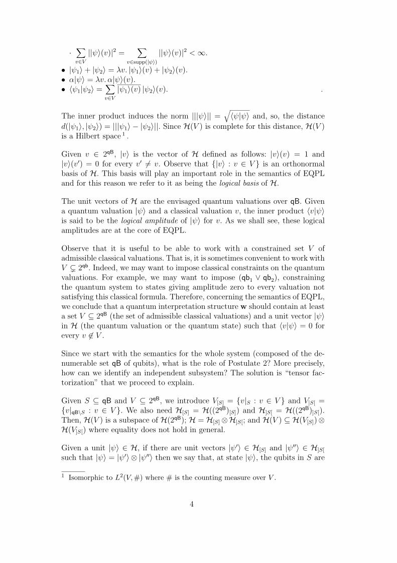
The inner product induces the norm |||ψ〉|| =√〈ψ|ψ〉 and, so, the distance

d(|ψ1〉, |ψ2〉) = |||ψ1〉 − |ψ2〉||. Since H(V ) is complete for this distance, H(V )is a Hilbert space 1 .

Given v ∈ 2qB, |v〉 is the vector of H defined as follows: |v〉(v) = 1 and|v〉(v′) = 0 for every v′ 6= v. Observe that |v〉 : v ∈ V is an orthonormalbasis of H. This basis will play an important role in the semantics of EQPLand for this reason we refer to it as being the logical basis of H.

The unit vectors of H are the envisaged quantum valuations over qB. Givena quantum valuation |ψ〉 and a classical valuation v, the inner product 〈v|ψ〉is said to be the logical amplitude of |ψ〉 for v. As we shall see, these logicalamplitudes are at the core of EQPL.

Observe that it is useful to be able to work with a constrained set V ofadmissible classical valuations. That is, it is sometimes convenient to work withV ( 2qb. Indeed, we may want to impose classical constraints on the quantumvaluations. For example, we may want to impose (qb1 ∨ qb2), constrainingthe quantum system to states giving amplitude zero to every valuation notsatisfying this classical formula. Therefore, concerning the semantics of EQPL,we conclude that a quantum interpretation structure w should contain at leasta set V ⊆ 2qB (the set of admissible classical valuations) and a unit vector |ψ〉in H (the quantum valuation or the quantum state) such that 〈v|ψ〉 = 0 forevery v 6∈ V .

Since we start with the semantics for the whole system (composed of the de-numerable set qB of qubits), what is the role of Postulate 2? More precisely,how can we identify an independent subsystem? The solution is “tensor fac-torization” that we proceed to explain.

Given S ⊆ qB and V ⊆ 2qB, we introduce V[S] = v|S : v ∈ V and V]S[ =v|qB\S : v ∈ V . We also need H[S] = H((2qB)[S]) and H]S[ = H((2qB)]S[).Then, H(V ) is a subspace of H(2qB); H = H[S]⊗H]S[; and H(V ) ⊆ H(V[S])⊗H(V]S[) where equality does not hold in general.

Given a unit |ψ〉 ∈ H, if there are unit vectors |ψ′〉 ∈ H[S] and |ψ′′〉 ∈ H]S[

such that |ψ〉 = |ψ′〉 ⊗ |ψ′′〉 then we say that, at state |ψ〉, the qubits in S are

1 Isomorphic to L2(V,#) where # is the counting measure over V .

4

not entangled with those outside S. In this situation, the state |ψ〉 is said to beS-factorizable. Furthermore, a vector |ψ〉 ∈ H[S] is said to be non-factorizableif there is no proper subset S ′ of S such that there are unit |ψ′〉 ∈ H[S′] andunit |ψ′′〉 ∈ H[S\S′] such that |ψ〉 = |ψ′〉 ⊗ |ψ′′〉.

Having in mind these semantic notions, given a finite set F of qubit symbols,we conclude that the language of EQPL should provide the means for writingassertions about:

• non-entanglement: “the qubits in F are not entangled with the other qubits”(that is, the quantum state at hand is F -factorizable); this assertion is made,as we shall see, with the EQPL formula [F ];

• logical amplitudes: “the amplitude of a classical valuation over F is equalto a complex number”; that is, we need terms denoting arbitrary complexnumbers and terms denoting logical amplitudes; more precisely, as we shallsee, when the quantum state is F -factorizable, the EQPL term |>〉FA de-notes the amplitude of the (unique) classical valuation vF

A over target Fthat satisfies the qubits in A ⊆ F and does not satisfy the qubits in F \A.

Other useful quantum constructions will be introduced as abbreviations, in-cluding inter alia:

• [G|F ] – formula stating that the quantum state is G-factorizable if it isF -factorizable.

• |α〉FA – term roughly denoting the amplitude of vFA if this classical valuation

satisfies α, and equal to zero otherwise.• ([F ]3 α : u) – formula stating that the quantum state is F -factorizable and

that there is a classical valuation v over F in the F -component of the quan-tum state satisfying α such that |v〉[F ] has non-null amplitude u.

Unfortunately, the amplitude terms are not always meaningful on a givenpair (V, |ψ〉). Namely, they require that the target qubits are not entangledwith the others. Therefore, we need more information in the envisaged notionof quantum interpretation structure. But, before we are ready to give thedefinition, we need some additional notation about partitions of qB. Given apartition S of qB, let ∪S be the set of all unions of elements of S. That is,∪S = ⋃S∈R S : R ⊆ S.

Definition 2.2 A quantum interpretation structure is a tuple

w = (V,S, |ψ〉, ν)

where:

• V is a nonempty subset of 2qB.• S is a finite partition of qB.

5

• |ψ〉 = |ψ〉[R]R∈∪S where each |ψ〉[R] is a unit vector of H[R] and such that:

(1) |ψ〉[∅] = ei0;(2) |ψ〉[R] = ⊗

S ∈ SS ⊆ R

|ψ〉[S] for each non-empty R ∈ ∪S;

(3) |ψ〉[S] is non-factorizable for each S ∈ S;(4) 〈v|ψ〉[qB] = 0 if v 6∈ V .

• ν : νFAF⊆finqB,A⊆F where each νFA ∈ C and νFA = 〈vFA |ψ〉[F ] if F ∈ ∪S. .

In such a structure, we recognize the key elements V (the set of admissi-ble classical valuations) and |ψ〉[qB] (the quantum state of the whole system).The additional information is the factorization of |ψ〉[qB] and the map ν thatprovides the means for interpreting amplitude terms even when they are phys-ically undefined. In this way we avoided the need to work with partial inter-pretation structures. Observe also that, although we work in H = H(2qB),clause 4 in the definition above imposes that (up to isomorphism) we onlyconsider quantum states in H(V ).

As we just saw, Postulates 1-2 were sufficient to guide us in the task of settingup the notion of quantum interpretation structure over which we shall be ableto define the semantics of EQPL. Now, we turn our attention to the postulatesconcerning measurements of physical quantities.

Postulate 3: Every measurable physical quantity of an isolated quantum sys-tem is described by an observable acting on its Hilbert space.

Recall that an observable is a Hermitian operator such that the direct sumof its eigensubspaces coincides with the underlying Hilbert space. Since theoperator is Hermitian, its spectrum Ω (the set of its eigenvalues) is a subsetof R. For each e ∈ Ω, we denote the corresponding eigensubspace by Ee andthe projector onto Ee by Pe.

Postulate 4: The possible outcomes of the measurement of a physical quantityare the eigenvalues of the corresponding observable. When the physical quan-tity is measured using observable A on a system in a state |ψ〉, the resultingoutcomes are ruled by the probability space PA

|ψ〉 = (Ω,B|Ω, µA|ψ〉) where in the

case of a countable spectrum

µA|ψ〉 = λB.

∑

e∈Ω

χB(e)‖Pe|ψ〉‖2 .

For the applications we have in mind in quantum computation and infor-mation, only logical projective measurements over a finite set of qubits arerelevant. Given a quantum structure w = (V,S, |ψ〉, ν), for each finite set F ofqubits, such measurements are defined using some observable AF on H suchthat:

6

• The spectrum of AF is equipotent 2 to V[F ].• For each v′ ∈ V[F ], the corresponding eigenspace Ev′ is generated by all

vectors of the form |v′〉⊗|v′′〉 inH. Thus, each projector Pv′ is |v′〉〈v′|⊗1H]F [.

For example, if the system is in the particular state

α00ω1|00ω1〉+ α01ω2|01ω2〉+ α01ω3|01ω3〉+ α10ω4|10ω4〉

then the probability of observing the first two qubits qb0, qb1 in the classicalvaluation 01 is given by |α01ω2|2 + |α01ω3|2.

In general, the stochastic result of making a logical projective measurement ofa finite set F of qubits of the system at w = (V,S, |ψ〉, ν) is fully described bythe finite probability space PF

w = (V[F ], ℘V[F ], µFw) where, for each U ⊆ V[F ]:

µFw(U) =

∑

v′∈U

∑

v′′∈V]F [

|〈(v′ ⊕ v′′)|ψ〉|2 .

Here, v′⊕v′′ denotes the (unique) classical valuation over all qubits determinedby v′ and v′′.

Thus, we are able to say what is the probability in a given quantum stateof observing a classical formula α as being true. That is, given a quantumstructure w, we have the means for interpreting EQPL terms of the form (

∫α)

that denote such probabilities.

Finally, although irrelevant to the design of EQPL, we mention en passantPostulate 5 that rules how quantum systems evolve.

Postulate 5: Excluding measurements, the evolution of a quantum system isdescribed by unitary transformations.

This last postulate becomes relevant only when designing a dynamical exten-sion of EQPL (see [2]).

2 The chosen bijection depends on how the qubits are physically implemented. Forexample, when implementing a qubit using the spin of an electron, we may imposethat spin +1

2 corresponds to true and spin −12 corresponds to false. But, as we shall

see, the semantics of EQPL does not depend on the choice of the bijection, as longas one exists. The same happens in the case of classical logic – its semantics doesnot depend on how bits are implemented. The details of which voltages correspondto which truth values are irrelevant.

7

3 Language and semantics

The language of EQPL is composed of classical formulae, real terms, complexterms and quantum formulae that we introduce using an abstract version ofthe BNF notation [21] for a compact presentation of inductive definitions.

Classical formulae:

α := qb 8⊥ 8 (α⇒ α)

As usual, we introduce through abbreviations other classical connectives like¬,∧,∨,⇔, as well as >. For instance, (¬α) is an abbreviation of (α ⇒ ⊥)and > stands for (¬⊥). We denote the set of qubit symbols occurring in α byqB(α). We say that a classical formula α is over a set S of qubit symbols ifqB(α) ⊆ S.

For building terms, it is convenient to use real variables X = xk : k ∈ Nand complex variables Z = zk : k ∈ N. Real and complex terms (with theprovisos computable real constant 3 r, finite F ⊂ qB and A ⊆ F ):

t := x 8 r 8 (∫α) 8 (t + t) 8 (t t) 8 Re(u) 8 Im(u) 8 arg(u) 8 |u|

u := z 8 |>〉FA 8 (t + it) 8 teit 8 u 8 (u + u) 8 (uu) 8 (α ¤ u; u)

Most of these terms are self-explanatory or already motivated in the previoussection. An explanation is needed concerning complex alternative terms: aterm (α ¤ u1; u2) denotes the value denoted by u1 if α is true, and denotesthe value denoted by u2 otherwise.

Quantum formulae (with the proviso finite F ⊂ qB):

γ := α 8 (t ≤ t) 8 [F ] 8 (γ A γ)

Quantum implication A is a global operator and should not be confused withits classical (local) counterpart. As expected, other quantum connectives willbe introduced as abbreviations. But, before introducing the whole set of usefulabbreviations, we present the semantics of the language.

Given a set S of qubit symbols and a set V of valuations, the extent at V ofclassical formulae over S is as follows (denoting classical satisfaction by °c):

• |α|SV = v ∈ V[S] : v °c α.

3 Following [22], we say that r is a computable real constant if there is a totalcomputable function f : N → Q such that |r − f(n)| ≤ 1/2n for every n ∈ N.Therefore, the set of such constants is countable.

8

By an assignment ρ, we mean a map such that ρ(x) ∈ R for each x ∈ X andρ(z) ∈ C for each z ∈ Z.

The denotation of terms at w = (V,S, |ψ〉, ν) and ρ is inductively defined asfollows:

• [[x]]wρ = ρ(x);• [[r]]wρ = r;

• [[(∫α)]]wρ = µqB(α)

w (|α|qB(α)V );

• [[z]]wρ = ρ(z);• [[|>〉FA]]wρ = νFA;

• [[(α ¤ u1; u2)]]wρ =

[[u1]]wρ if wρ ° α

[[u2]]wρ otherwise;

The denotation of the other terms follow the same lines. For instance,

• [[t1 + t2]]wρ = [[t1]]wρ + [[t2]]wρ.

The satisfaction of quantum formulae at w = (V,S, |ψ〉, ν) and ρ is inductivelydefined as follows:

• wρ ° α iff v °c α for every v ∈ V ;• wρ ° (t1 ≤ t2) iff [[t1]]wρ ≤ [[t2]]wρ;• wρ ° [F ] iff F ∈ ∪S;• wρ ° (γ1 A γ2) iff wρ 6° γ1 or wρ ° γ2.

The exogenous nature of the proposed semantics plays a double role above.First, the denotation of a probability term (

∫α) is the measure of the extent of

α, that is, the measure of the set of classical valuations that satisfy the classicalformula α. Second, a classical formula is satisfied by a quantum structure(roughly a superposition of classical valuations) if all those classical valuationssatisfy the formula.

As anticipated in the previous section, the proposed quantum language withthe semantics above is rich enough to express interesting properties of quan-tum systems. To this end, it is quite useful to introduce other operations,connectives and modalities through abbreviations. We start with some addi-tional quantum connectives:

• quantum negation: (¯ γ) for (γ A⊥);• quantum disjunction: (γ1 t γ2) for ((¯ γ1) A γ2);• quantum conjunction: (γ1 u γ2) for (¯((¯ γ1) t (¯ γ2)));• quantum equivalence: (γ1 ≡ γ2) for ((γ1 A γ2) u (γ2 A γ1)).

Observe that the quantum connectives are classical in the sense that quantum

9

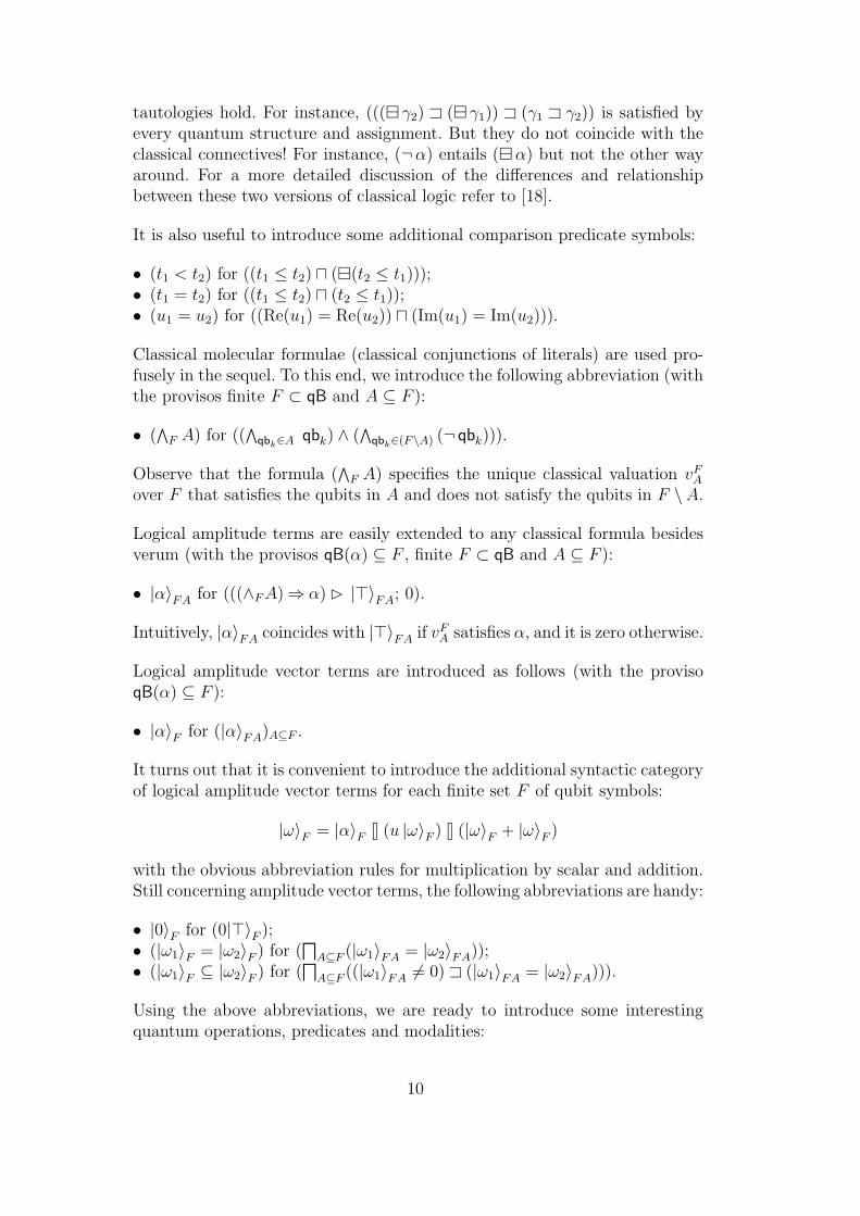
tautologies hold. For instance, (((¯ γ2) A (¯ γ1)) A (γ1 A γ2)) is satisfied byevery quantum structure and assignment. But they do not coincide with theclassical connectives! For instance, (¬α) entails (¯ α) but not the other wayaround. For a more detailed discussion of the differences and relationshipbetween these two versions of classical logic refer to [18].

It is also useful to introduce some additional comparison predicate symbols:

• (t1 < t2) for ((t1 ≤ t2) u (¯(t2 ≤ t1)));• (t1 = t2) for ((t1 ≤ t2) u (t2 ≤ t1));• (u1 = u2) for ((Re(u1) = Re(u2)) u (Im(u1) = Im(u2))).

Classical molecular formulae (classical conjunctions of literals) are used pro-fusely in the sequel. To this end, we introduce the following abbreviation (withthe provisos finite F ⊂ qB and A ⊆ F ):

• (∧

F A) for ((∧

qbk∈A qbk) ∧ (∧

qbk∈(F\A) (¬ qbk))).

Observe that the formula (∧

F A) specifies the unique classical valuation vFA

over F that satisfies the qubits in A and does not satisfy the qubits in F \A.

Logical amplitude terms are easily extended to any classical formula besidesverum (with the provisos qB(α) ⊆ F , finite F ⊂ qB and A ⊆ F ):

• |α〉FA for (((∧F A)⇒ α) ¤ |>〉FA; 0).

Intuitively, |α〉FA coincides with |>〉FA if vFA satisfies α, and it is zero otherwise.

Logical amplitude vector terms are introduced as follows (with the provisoqB(α) ⊆ F ):

• |α〉F for (|α〉FA)A⊆F .

It turns out that it is convenient to introduce the additional syntactic categoryof logical amplitude vector terms for each finite set F of qubit symbols:

|ω〉F = |α〉F 8 (u |ω〉F ) 8 (|ω〉F + |ω〉F )

with the obvious abbreviation rules for multiplication by scalar and addition.Still concerning amplitude vector terms, the following abbreviations are handy:

• |0〉F for (0|>〉F );• (|ω1〉F = |ω2〉F ) for (

dA⊆F (|ω1〉FA = |ω2〉FA));

• (|ω1〉F ⊆ |ω2〉F ) for (d

A⊆F ((|ω1〉FA 6= 0) A (|ω1〉FA = |ω2〉FA))).

Using the above abbreviations, we are ready to introduce some interestingquantum operations, predicates and modalities:

10

• [G|F ] for (d

A′⊆G

dA′′⊆F\G (|>〉F (A′A′′) = |>〉GA′|>〉(F\G)A′′)) with G ⊆ F ;

• (qbk1∼F qbk2

) for (¯(⊔

G ⊂ Fqbk1

∈ Gqbk2

/∈ G

[G]));

• ([F ]3 α : u) for ([F ] u |u| > 0 u (⊔

A⊆F (|α〉FA = u)));• ([F ]3 α1 : u1, . . . , αn : un) for (([F ]3 α1 : u1) u . . . u ([F ]3 αn : un));• (3α) for (0 < (

∫α));

• (2α) for (1 = (∫α)).

Most of these quantum constructions were already discussed in the previoussection. The entanglement formula (qbk1

∼F qbk2) states that the two qubits

are entangled.

Quantum molecular formulae (quantum conjunctions of literals) are also veryuseful. Note that a quantum literal is either a quantum atom or the quantumnegation of a quantum atom. Looking at the grammar of quantum formulae,it is clear that quantum atoms are either classical formulae, or comparisonsbetween real terms or non-entanglement assertions:

qAtom := α 8 (t ≤ t) 8 [F ]

Finally, we introduce the following abbreviation (with the provisos finite Q ⊂qAtom and D ⊆ Q) that will be used extensively in the proof of completeness:

• (d

Q D) for ((d

δ∈D δ) u (d

δ∈(Q\D) (¯ δ))).

Observe that a quantum molecular formula defines a set of quantum structuresthat may be empty because, for instance, the quantum molecular formula(α u (¬α)) has no models (here Q = α, (¬α) = D).

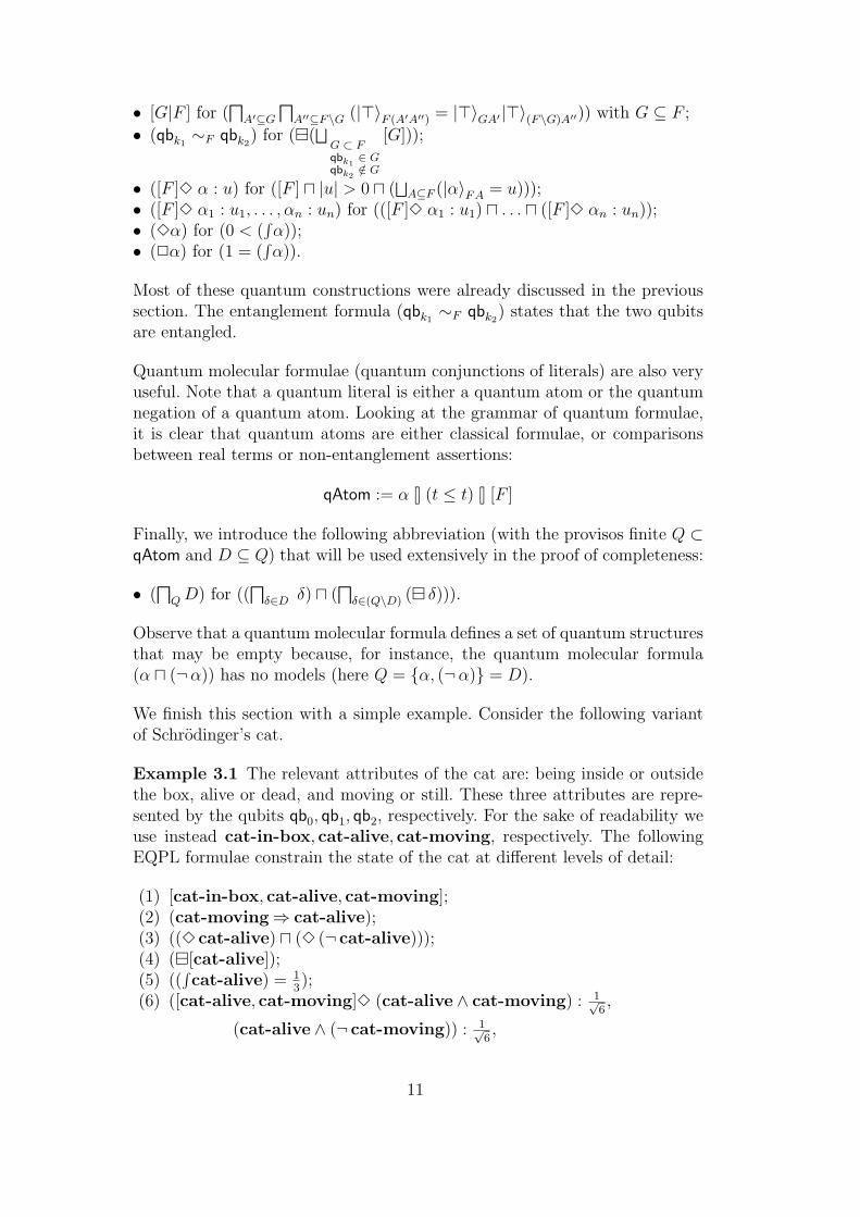
We finish this section with a simple example. Consider the following variantof Schrodinger’s cat.

Example 3.1 The relevant attributes of the cat are: being inside or outsidethe box, alive or dead, and moving or still. These three attributes are repre-sented by the qubits qb0, qb1, qb2, respectively. For the sake of readability weuse instead cat-in-box, cat-alive, cat-moving, respectively. The followingEQPL formulae constrain the state of the cat at different levels of detail:

(1) [cat-in-box, cat-alive, cat-moving];(2) (cat-moving⇒ cat-alive);(3) ((3 cat-alive) u (3 (¬ cat-alive)));(4) (¯[cat-alive]);(5) ((

∫cat-alive) = 1

3);

(6) ([cat-alive, cat-moving]3 (cat-alive ∧ cat-moving) : 1√6,

(cat-alive ∧ (¬ cat-moving)) : 1√6,

11

((¬ cat-alive) ∧ (¬ cat-moving)) : ei π3

√23).

Observe that the assertions above are consistent with each other. Intuitively,assertion 1 states that the qubits cat-in-box, cat-alive, cat-moving are notentangled with the other qubtis of the cat system. Assertion 2 is a classicalconstraint on the set of admissible valuations: if the cat is moving then it isalive. Assertion 3 states the famous paradox: the cat can be in a state where itis possible that the cat is alive and it is possible that the cat is dead. Assertion4 states that the qubit cat-alive is entangled with other qubits. Assertion 5states that the cat is in a state where the probability of observing it alive (aftercollapsing the wave function) is 1

3. Finally, assertion 6 states that the qubits

cat-alive, cat-moving are not entangled with other qubits and that in thequantum state there is a classical valuation with amplitude 1√

6where the cat

is alive and moving, there is another classical valuation also with amplitude1√6

where the cat is alive and not moving, and there is a classical valuation

with amplitude ei π3

√23

where the cat is dead (and, thus, thanks to 2, also not

moving). .

4 Axiomatization

Entailment for EQPL may be defined as expected – we say that Γ entails η,written Γ ² η, if wρ ° η for every w and ρ satisfying every element of Γ. Buta finitely bounded version of entailment turns out to be more relevant. Givena finite set F of qubit symbols, a quantum structure w = (V,S, ψ, ν) is saidto be F -factorizable if F ∈ ∪S. Given a set Γ of quantum formulae over Fand a quantum formula η also over F , we say that the former F -entails thelatter, written Γ ²F η if wρ ° η for every F -factorizable w and ρ satisfyingevery element of Γ.

Observe that Γ ² η implies Γ ²F η for every F . Furthermore, for any Γ andη over F1, if F1 ⊆ F2 and Γ ²F2 η then Γ ²F1 η. Note also that Γ, η1 ²F η2 iffΓ ²F (η1 A η2), and a similar result holds for the unbounded entailment. Thatis, quantum implication does internalize the notion of quantum entailment inEQPL.

Note also that both entailments (unbounded and bounded) are not compactin the sense that there are Γ and η such that η is entailed by Γ but it is notentailed by any finite subset of Γ. Indeed, (z = 0) is entailed from (|z| ≤1/n : n ∈ N). But, (z = 0) is not entailed by any finite subset of this set.

Therefore, there is no hope of setting up a finitary axiomatization (that is,using only finitary rules) achieving strong completeness. But, it is possible toestablish a finitary axiomatization that achieves F -bounded weak completeness

12

for any finite F : ²F η iff `F η. Indeed, the axioms and rules presented beloware sound and adequate for F -validity as will be proved in the next section.

Before listing all axioms and rules we need to introduce the concept of tau-tological quantum formula or quantum tautology. A quantum formula γ issaid to be tautological if there are a classical tautology α and a substitu-tion map σ : qB → qAtom such that γ coincides with α⇒A σ (where α⇒A isthe quantum formula obtained from α by replacing the classical connectivesby the corresponding quantum connectives). For instance, the quantum for-mula ((x1 ≤ x2) A (x1 ≤ x2)) is tautological (obtained, for example, from theclassical tautology (qb1 ⇒ qb1)).

We also need to identify the following sublanguage of EQPL that we shallhenceforth call analytical language:

κ := (a ≤ a) 8⊥ 8 (κ A κ)

a := x 8 r 8 (a + a) 8 (a a) 8 Re(b) 8 Im(b) 8 arg(b) 8 |b|b := z 8 (a + ia) 8 aeia 8 b 8 (b + b) 8 (b b)

Observe that an assignment ρ is enough to interpret formulae of this sub-language. Therefore, an analytical formula κ is valid iff it is satisfied byevery assignment. For instance, (((t1 ≤ t2) u (t2 ≤ t3)) A (t1 ≤ t3)) and((u2

1 = −1) A ((u1 = i) t (u1 = −i))) are both universal analytical formulae(the latter using equality between complex numbers introduced as an abbre-viation).

Proposition 4.1 The set of valid analytical formulae is not recursively enu-merable.

Indeed, assuming that the set is recursively enumerable we reach a contra-diction as follows. Let h be a computable enumeration of the valid analyticalformula. Consider the procedure:

n := 0;

b := True;

while b do if h(n) = (r = 0) then Output(True); b := Falseif h(n) = (r 6= 0) then Outputr(False); b := Falsen := n + 1

This procedure always terminates since either r = 0 or r 6= 0 is valid. Hence,

13

it is a decision algorithm for the problem “equality to zero of a computablereal constant”, contradicting the known undecidability of this problem (see4.23.3 of [22]).

We are now ready to list the axioms and rules of our calculus for each finiteset F of qubit symbols: see Table 1 4 .

`F α for each classical tautology α [CTaut]

α1, (α1 ⇒ α2) `F α2 [CMP]

`F γ for each quantum tautology γ [QTaut]

γ1, (γ1 A γ2) `F γ2 [QMP]

`F κ~x~z~t~u

for each valid analytical formula κ [Oracle]

`F ((α1 ⇒ α2) A (α1 A α2)) [Lift⇒]

`F ((α1 u α2) A (α1 ∧ α2)) [Refu]

`F (α A ((α ¤ u1; u2) = u1)) [If>]

`F ((¯α) A ((α ¤ u1; u2) = u2)) [If⊥]

`F [F ] [NEtgF ]

`F ([G2] A ([G1]≡ [G1|G2])) for any G1 ⊆ G2 [NEtg|]`F ([G1] A ([G2] A [G1 ∪G2])) [NEtg∪]

`F ([G1] A ([G2] A [G1 \G2])) [NEtg\]`F (|>〉∅∅ = 1) [Empty]

`F ((¬(∧F A)) A (|>〉FA = 0)) [NAdm]

`F ([G] A ((∑

A⊆G ||>〉GA|2) = 1)) [Unit]

`F ((∫

α) = (∑

A⊆F ||α〉FA|2)) [Prob].

Table 1Axiomatization of EQPL

In total, we have only two rules (modus ponens for classical implication [CMP]and for quantum implication [QMP] 5 ) and fifteen axiom schemas. The axiom

4 By κ~x~z~t~u

we mean the formula obtained from κ by uniform and simultaneous substi-tution of the variables ~x = xi1 , . . . , xin and ~z = zi1 , . . . , zim by terms ~t = ti1 , . . . , tinand ~u = ui1 , . . . , uim , respectively.5 Actually, [CMP] can be derived from [QMP] and [Lift⇒].

14

schemas are better understood in the following groups.

We have as axiom schemas the classical tautologies and the quantum tau-tologies ([CTaut] and [QTaut], respectively). This is justified by the fact thatthe set of classical tautologies and the set of quantum tautologies are bothrecursive.

Since the set of valid analytical formulae is not recursively enumerable and,thus, not recursive, Axiom schema [Oracle] is controversial. We decided touse an analytical oracle for two reasons. First, we wanted to focus our atten-tion on reasoning about quantum aspects without becoming lost in analyticaldetails. And, second, the alternative of presenting a recursive axiomatizationbased on the theory of real closed fields and their algebraic closures would re-quire a much weaker language (without computable real constants and withoutexponentiation) and, in order to maintain completeness, a relaxation of oursemantics, maybe towards a point too far away from its intuitive roots in thepostulates of quantum mechanics. However, this alternative is interesting alsofor other reasons and we shall come back to the issue in the last section of thepaper.

Axiom schemas [Lif⇒] and [Refu] are sufficient to relate (local) classical rea-soning and (global) quantum tautological reasoning. Again, we refer to [18]for more details.

Axiom schemas [If>] and [If⊥] are self explanatory. They will be used in thecompleteness proof to remove alternative terms.

Axiom schemas [NEtgF ], [NEtg|], [NEtg∪] and [NEtg\] are enough to rea-son about non-entanglement. Among other things they impose that non-entanglement is closed under set theoretic operations (closure under inter-section appears as a theorem as we shall see).

Axiom schemas [Empty], [NAdm] and [Unit] rule logical amplitudes. Each ofthem closely reflects a property of our semantic structures.

Finally, [Prob] relates probabilities and amplitudes, closely following Postulate4 of quantum mechanics.

As expected, we say that a formula η over F is F -derivable from a set Γ offormulae over F , written Γ `F η if we can build a derivation of η from theaxioms and the elements of Γ using the inference rules. Furthermore, we saythat a formula η over F is an F -theorem, written `F η if it is F -derivablefrom the empty set. As an illustration, consider the derivation in Table 2 thatestablishes for any finite F :

• `F ((∫>) = 1) [PUnit].

15

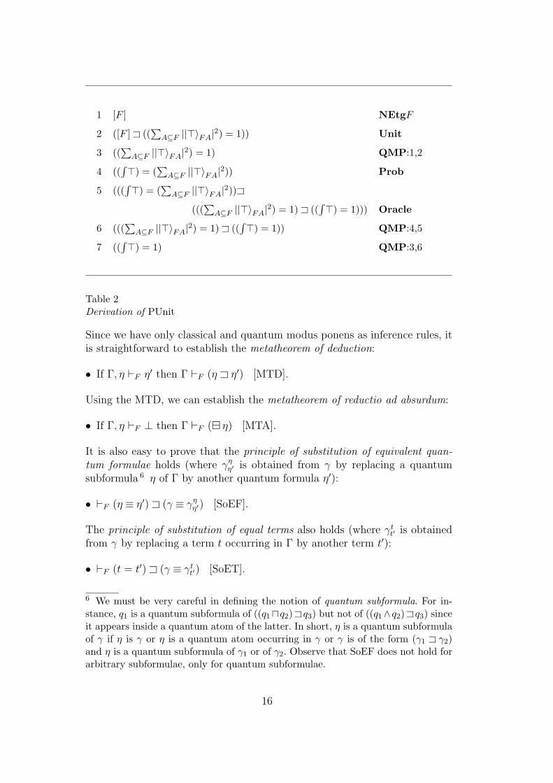
1 [F ] NEtgF

2 ([F ] A ((∑

A⊆F ||>〉FA|2) = 1)) Unit

3 ((∑

A⊆F ||>〉FA|2) = 1) QMP:1,2

4 ((∫>) = (

∑A⊆F ||>〉FA|2)) Prob

5 (((∫>) = (

∑A⊆F ||>〉FA|2))A

(((∑

A⊆F ||>〉FA|2) = 1) A ((∫>) = 1))) Oracle

6 (((∑

A⊆F ||>〉FA|2) = 1) A ((∫>) = 1)) QMP:4,5

7 ((∫>) = 1) QMP:3,6

Table 2Derivation of PUnit

Since we have only classical and quantum modus ponens as inference rules, itis straightforward to establish the metatheorem of deduction:

• If Γ, η `F η′ then Γ `F (η A η′) [MTD].

Using the MTD, we can establish the metatheorem of reductio ad absurdum:

• If Γ, η `F ⊥ then Γ `F (¯ η) [MTA].

It is also easy to prove that the principle of substitution of equivalent quan-tum formulae holds (where γη

η′ is obtained from γ by replacing a quantumsubformula 6 η of Γ by another quantum formula η′):

• `F (η ≡ η′) A (γ ≡ γηη′) [SoEF].

The principle of substitution of equal terms also holds (where γtt′ is obtained

from γ by replacing a term t occurring in Γ by another term t′):

• `F (t = t′) A (γ ≡ γtt′) [SoET].

6 We must be very careful in defining the notion of quantum subformula. For in-stance, q1 is a quantum subformula of ((q1uq2)Aq3) but not of ((q1∧q2)Aq3) sinceit appears inside a quantum atom of the latter. In short, η is a quantum subformulaof γ if η is γ or η is a quantum atom occurring in γ or γ is of the form (γ1 A γ2)and η is a quantum subformula of γ1 or of γ2. Observe that SoEF does not hold forarbitrary subformulae, only for quantum subformulae.

16

1 (α1 ∧ α2)⇒ α1 CTaut

2 ((α1 ∧ α2)⇒ α1) A ((α1 ∧ α2) A α1) Lift⇒3 (α1 ∧ α2) A α1 QMP:1,2

4 (α1 ∧ α2)⇒ α2 CTaut

5 ((α1 ∧ α2)⇒ α2) A ((α1 ∧ α2) A α2) Lift⇒6 (α1 ∧ α2) A α2 QMP:4,5

7 ((α1 ∧ α2) A α1)A

(((α1 ∧ α2) A α2) A ((α1 ∧ α2) A (α1 u α2))) QTaut

8 ((α1 ∧ α2) A α2) A ((α1 ∧ α2) A (α1 u α2)) QMP:3,7

9 (α1 ∧ α2) A (α1 u α2) QMP:6,8

Table 3Derivation of Lift∧We finish this section with a list of interesting F -theorems. Some of them willbe needed in the proof of weak completeness presented in the next section(and for this reason we provide their derivations), but others are mentionedjust for illustration purposes.

First, observe that we have as theorems the following lifting properties thatwe shall use in the proof of completeness.

In Table 3 is a derivation of the lifting of conjunction:

• `F ((α1 ∧ α2) A (α1 u α2)) [Lift∧].

The derivation of the lifting of negation

• `F ((¬α) A (¯ α)) [Lift¬].

is trivial since it is a special case of Axiom Lift⇒.

The following theorem, derived in Table 4 using MTD, completes the pictureof non-entanglement being closed under set theoretic operations.

• `F ([G1] A ([G2] A [G1 ∩G2])) [NEtg∩].

The following theorems give some insight on the major properties of logical

17

1 [F ] NEtgF

2 ([F ] A ([G1] A [F \G1])) NEtg\3 ([G1] A [F \G1]) QMP:1,2

4 [G1] Hyp

5 [F \G1] QMP:4,3

6 ([F ] A ([G2] A [F \G2])) NEtg\7 ([G2] A [F \G2]) QMP:1,6

8 [G2] Hyp

9 [F \G2] QMP:8,7

10 ([F \G1] A ([F \G2] A [(F \G1) ∪ (F \G2)])) NEtg∪11 ([F \G2] A [(F \G1) ∪ (F \G2)]) QMP:5,10

12 [(F \G1) ∪ (F \G2)] QMP:9,11

13 ([F ] A ([(F \G1) ∪ (F \G2)] A [G1 ∩G2])) NEtg\14 ([(F \G1) ∪ (F \G2)] A [G1 ∩G2]) QMP:1,13

15 [G1 ∩G2] QMP:12,14

Table 4Derivation of NEtg∩

amplitudes and how they are related with the (classical and quantum) con-nectives.

• `F ((|(α1 ∨ α2)〉G + |(α1 ∧ α2)〉G) = (|α1〉G + |α2〉G)) [AAdd].• `F ((α1 ⇒ α2) A (|α1〉G ⊆ |α2〉G)) [AMon].• `F ((α1 ⇔ α2) A (|α1〉G = |α2〉G)) [ASoE].• `F (α A (|α〉G = |>〉G)) [ANec].• `F ((|α〉G + |(¬α)〉G) = |>〉G) [AMExc].

The first of the following theorems about probability after measurements juststates finite additivity. The second is an obvious instance of Postulate 4. Thethird relates logical reasoning with probability reasoning (monotonicity).

• `F (((∫(α1 ∨ α2)) + (

∫(α1 ∧ α2))) = ((

∫α1) + (

∫α2))) [PAdd].

• `F (([G]3 (∧

G A) : u) A ((∫(∧

G A)) = |u|2)) [Meas].• `F ((α1 ⇒ α2) A ((

∫α1) ≤ (

∫α2))) [PMon].

18

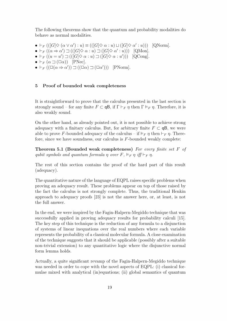
The following theorems show that the quantum and probability modalities dobehave as normal modalities.

• `F (([G]3 (α ∨ α′) : u)≡ (([G]3 α : u) t ([G]3 α′ : u))) [QNorm].• `F ((α⇒ α′) A (([G]3 α : u) A ([G]3 α′ : u))) [QMon].• `F ((u = u′) A (([G]3 α : u) A ([G]3 α : u′))) [QCong].• `F (α A (2α)) [PNec].• `F ((2(α⇒ α′)) A ((2α) A (2α′))) [PNorm].

5 Proof of bounded weak completeness

It is straightforward to prove that the calculus presented in the last section isstrongly sound – for any finite F ⊂ qB, if Γ `F η then Γ ²F η. Therefore, it isalso weakly sound.

On the other hand, as already pointed out, it is not possible to achieve strongadequacy with a finitary calculus. But, for arbitrary finite F ⊂ qB, we wereable to prove F -bounded adequacy of the calculus – if ²F η then `F η. There-fore, since we have soundness, our calculus is F -bounded weakly complete:

Theorem 5.1 (Bounded weak completeness) For every finite set F ofqubit symbols and quantum formula η over F , ²F η iff `F η.

The rest of this section contains the proof of the hard part of this result(adequacy).

The quantitative nature of the language of EQPL raises specific problems whenproving an adequacy result. These problems appear on top of those raised bythe fact the calculus is not strongly complete. Thus, the traditional Henkinapproach to adequacy proofs [23] is not the answer here, or, at least, is notthe full answer.

In the end, we were inspired by the Fagin-Halpern-Megiddo technique that wassuccessfully applied in proving adequacy results for probability calculi [15].The key step of this technique is the reduction of any formula to a disjunctionof systems of linear inequations over the real numbers where each variablerepresents the probability of a classical molecular formula. A close examinationof the technique suggests that it should be applicable (possibly after a suitablenon-trivial extension) to any quantitative logic where the disjunctive normalform lemma holds.

Actually, a quite significant revamp of the Fagin-Halpern-Megiddo techniquewas needed in order to cope with the novel aspects of EQPL: (i) classical for-mulae mixed with analytical (in)equations; (ii) global semantics of quantum

19

connectives; (iii) non-entanglement atoms; (iv) amplitude terms besides prob-ability terms; and (v) quantum structures instead of probability spaces. Notethat the Fagin-Halpern-Meggido technique was first developed for a proba-bilistic logic somewhat simpler than the probabilistic fragment of EQPL.

In addition, we used the Henkin technique thrice: (i) for removing alterna-tive terms; (ii) for constructing the set of admissible valuations; and (iii) forbuilding the finite partition of the set of qubits.

After these comments on the overall strategy, we are now ready to start the(top-down) proof of the F -bounded weak adequacy of EQPL.

Given a quantum formula γ over F we say that it is F -consistent if 6`F (¯ γ).

The proof is carried out by contraposition:

(1) Assume that 6`F γ.(2) So, quantum tautologically, also 6`F (¯(¯ γ)).(3) Thus, (¯ γ) is F -consistent.(4) Therefore, by the model existence lemma proved below, there are F -

factorizable w and ρ such that wρ ° (¯ γ).(5) And, hence, it is not true that every such pair satisfies γ, that is, we

established that 6²F γ.

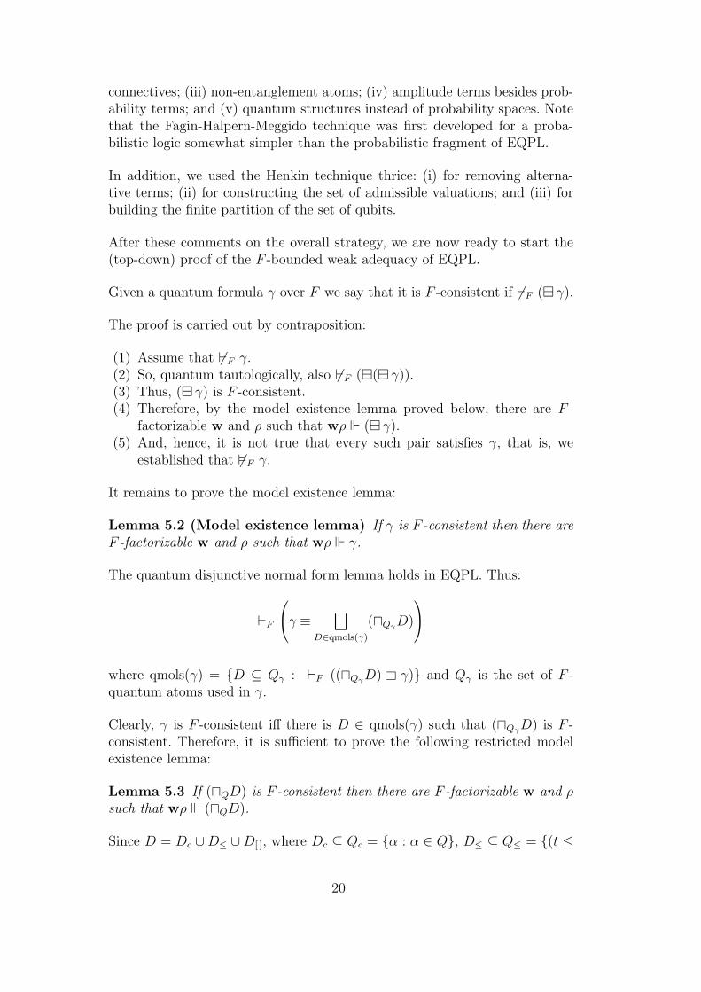
It remains to prove the model existence lemma:

Lemma 5.2 (Model existence lemma) If γ is F -consistent then there areF -factorizable w and ρ such that wρ ° γ.

The quantum disjunctive normal form lemma holds in EQPL. Thus:

`F

γ ≡ ⊔

D∈qmols(γ)

(uQγD)

where qmols(γ) = D ⊆ Qγ : `F ((uQγD) A γ) and Qγ is the set of F -quantum atoms used in γ.

Clearly, γ is F -consistent iff there is D ∈ qmols(γ) such that (uQγD) is F -consistent. Therefore, it is sufficient to prove the following restricted modelexistence lemma:

Lemma 5.3 If (uQD) is F -consistent then there are F -factorizable w and ρsuch that wρ ° (uQD).

Since D = Dc ∪D≤ ∪D[ ], where Dc ⊆ Qc = α : α ∈ Q, D≤ ⊆ Q≤ = (t ≤

20

t′) : (t ≤ t′) ∈ Q, and D[ ] ⊆ Q[ ] = [G] : [G] ∈ Q, we have:

(uQD) = ((uQcDc) u (uQ≤D≤) u (uQ[ ]D[ ])).

Our goal is to reduce everything to inequations. We start by getting rid of thenon-entanglement atoms.

Thanks to NEtgF and NEtg|, we know that there is a quantum formula δ[]

without non-entanglement atoms such that `F ((uQ[ ]D[ ]) ≡ δ[ ]). Thus, `F

((uQD)≡ δ) where δ = ((uQcDc) u (uQ≤D≤) u δ[ ]).

Note that δ[ ] and, hence, δ are not necessarily conjunctions of quantum literals(because it may happen that a [G] appears in Q[ ] \ D[ ] and such a negationinvolves a disjunction). Using again the quantum disjunctive normal formlemma we have:

`F

δ ≡ ⊔

D∈qmols(δ)

(uQδD)

.

So, δ is F -consistent iff there is D ∈ qmols(δ) such that (uQδD) is F -consistent.

Therefore, it is sufficient to prove the following even more restricted modelexistence lemma:

Lemma 5.4 If (uQD) without entanglement atoms is F -consistent then thereare F -factorizable w and ρ such that wρ ° (uQD).

Assume that (uQD) is F -consistent and does not involve non-entanglementatoms (that is, Q = Qc ∪ Q≤ and D = Dc ∪ D≤). Our goal is to find an F -factorizable w = (V,S, |ψ〉, ν) and a ρ satisfying this molecular formula. Westart by looking for V .

Before setting up V , it is necessary to eliminate the probability and alterna-tive terms and to add maximally consistent information about the admissibleclassical valuations. This desideratum is achieved as follows:

(1) First, we replace in (uQD) each term (∫α) by

∑A⊆F ||α〉FA|2. Let (uQD)

be the result.(2) Consider an ordering α1, . . . , αm of the guards of alternative terms occur-

ring in (uQD).(3) Consider the following sequence of formulae:

• η0 = (uQD);

• ηk+1 =

(ηk u αk) if `F (ηk A αk)

(ηk u (¯ αk)) otherwise.

(4) Observe that each ηk is still F -consistent and a quantum molecular for-mula. Furthermore, ηm is maximal with respect to guards.

(5) Now we can replace each term (α ¤ u1; u2) occurring in ηm by:

21

• u1 if α is a quantum literal in ηm;• u2 if (¯ α) is a quantum literal in ηm.Let ηm be the resulting formula.

(6) Consider an ordering A1, . . . , Am′ of the subsets of F .(7) Consider the following sequence of formulae:

• η′0 = ηm;

• η′k+1 =

(η′k u (¬(∧F Ak))) if `F (η′k A (¬(∧F Ak)))

(η′k u (¯(¬(∧F Ak)))) otherwise.

(8) Observe that each η′k is still F -consistent and a quantum molecular for-mula. Furthermore, η′m′ does not contain probability terms or alternativeterms and is maximal with respect to admissible classical valuations.

(9) Thanks to Prob, If> and If⊥, denoting the resulting still F -consistentmolecular formula by (uQ′D

′) = ((uQ′cD′c) u (uQ′≤D′

≤)), we have

`F ((uQ′D′) A (uQD)).

(10) Therefore, we may proceed working towards the envisaged w and ρ withthe new formula.

Having (while preserving F -consistency) eliminated the probability and alter-native terms and having determined the classical valuations, we are ready tobuild V . Let V be composed of each v ∈ 2qB

[F ] such that v °c α for each α ∈ D′c.

Now we have to analyze two cases:

a) Either for each α ∈ Q′c\D′

c there is a v ∈ V such that v 6°c α and, therefore,this V is viable because

(V, . . . ) °F (uQ′cD′c) .

b) Or that is not the case. But, then, we would be able to contradict theF -consistency of (uQ′D

′) as follows:(1) Indeed, if it is not the case then there is a α ∈ Q′

c \D′c such that v °c α

for all v ∈ V . That is, by construction of V , there is α ∈ Q′c \D′

c suchthat

²c

∧

α′∈D′c

α′⇒ α

.

(2) So, by CTaut, there is α ∈ Q′c \D′

c such that

`F

∧

α′∈D′c

α′⇒ α

.

(3) Thus, by Lift⇒, there is α ∈ Q′c \D′

c such that

`F

∧

α′∈D′c

α′ A α

.

22

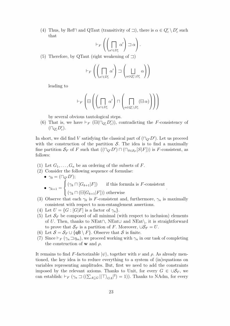
(4) Thus, by Refu and QTaut (transitivity of A), there is α ∈ Q′c \D′

c suchthat

`F

l

α′∈D′c

α′ A α

.

(5) Therefore, by QTaut (right weakening of A)

`F

l

α′∈D′c

α′ A

⊔

α∈Q′c\D′cα

leading to

`F

¯

l

α′∈D′c

α′ u

l

α∈Q′c\D′c(¯ α)

by several obvious tautological steps.(6) That is, we have `F (¯(uQ′cD

′c)), contradicting the F -consistency of

(uQ′cD′c).

In short, we did find V satisfying the classical part of (uQ′D′). Let us proceed

with the construction of the partition S. The idea is to find a maximallyfine partition SF of F such that ((uQ′D

′) u (uS∈SF[S|F ])) is F -consistent, as

follows:

(1) Let G1, . . . , Gn be an ordering of the subsets of F .(2) Consider the following sequence of formulae:

• γ0 = (uQ′D′);

• γk+1 =

(γk u [Gk+1|F ]) if this formula is F -consistent

(γk u (¯[Gk+1|F ])) otherwise.

(3) Observe that each γk is F -consistent and, furthermore, γn is maximallyconsistent with respect to non-entanglement assertions.

(4) Let U = G : [G|F ] is a factor of γn.(5) Let SF be composed of all minimal (with respect to inclusion) elements

of U . Then, thanks to NEnt∩, NEnt∪ and NEnt\, it is straightforwardto prove that SF is a partition of F . Moreover, ∪SF = U .

(6) Let S = SF ∪ qB \ F. Observe that S is finite.(7) Since `F (γn Aηm), we proceed working with γn in our task of completing

the construction of w and ρ.

It remains to find F -factorizable |ψ〉, together with ν and ρ. As already men-tioned, the key idea is to reduce everything to a system of (in)equations onvariables representing amplitudes. But, first we need to add the constraintsimposed by the relevant axioms. Thanks to Unit, for every G ∈ ∪SF , wecan establish: `F (γn A ((

∑A⊆G ||>〉GA|2) = 1)). Thanks to NAdm, for every

23

(¬(∧F A)) occurring in γn, we have: `F (γn A (|>〉FA = 0)).

Let γ•n be the formula

γn u

lG∈∪SF

∑

A⊆G

||>〉GA|2 = 1

u

l

(¬(∧F A)) in γn

(|>〉FA = 0)

.

Observe that we can derive: `F (γn ≡ γ•n). Let (γ•n)≤ the conjunction of the(in)equations in γ•n. Consider the finite system of (in)equations obtained from(γ•n)≤ by replacing at each term of the form |>〉GA by a fresh variable z|>〉GA

.Now we have to analyse two cases:

a) Either the system of (in)equations has no solution. But, in this case wewould be able to contradict the F -consistency of γn as follows (using theanalytical oracle):(1) Let Λ≤ be the (finite) set of analytical literals occurring in (γ•n)≤ and

Λc be the (finite) set of non-analytical literals in (γ•n)c.(2) Since (γ•n)≤ = (uκ∈Λ≤κ), there is a bijection between Λ≤ and the set of

inequations composing the system described above.(3) From the fact that the system of inequations induced by (γ•n)≤ has no

solution, we conclude that there is no assignment ρ such that ρ ° κ forall κ ∈ Λ≤.

(4) In other words, for all assignment ρ there exists κ ∈ Λ≤ such thatρ ° (¯κ) and so, thanks to Oracle, we have: `F (tκ∈Λ≤(¯ κ)).

(5) Hence, a fortiori, we obtain: `F ((tγ∈Λc(¯ γ)) t (tκ∈Λ≤(¯κ))).(6) That is, since

((tγ∈Λc(¯ γ)) t (tκ∈Λ≤(¯κ))) ≡ (¯((uγ∈Λcγ) u (uκ∈Λ≤κ)))

= (¯((γ•n)c u (γ•n)≤))

= (¯ γ•n)

≡ (¯ γn),

we can conclude `F (¯ γn), contradicting the F -consistency of γn.b) Or the system has at least one solution and then we can build the envisaged

F -factorizable w = (V,S, |ψ〉, ν) and ρ from any of the solutions in thefollowing way:• V is as described above.• S is as described above.• |ψ〉 = |ψ〉[R]R∈∪S is obtained as follows:

· |ψ〉[G](vGA) is the solution value of z|>〉GA

for every G ∈ SF (note that

24

|ψ〉[G] is non-factorizable by construction of SF );

· |ψ〉[qB\F ] is any non-factorizable unit vector in H(2qB[qB\F ]) such that

〈v|ψ〉[qB\F ] = 0 for every v 6∈ V[qB\F ];

· |ψ〉[∅] = ei0 and |ψ〉[R] = ⊗S ∈ SS ⊆ R

|ψ〉[S] for each non-empty R ∈ ∪S.

• ν = νGAG⊂finqB,A⊆G is chosen as follows:· If z|>〉GA

is a variable of the system then νGA takes the value of thisvariable in the adopted solution.

· Otherwise:If G ∈ SF then νGA = 〈vG

A |ψ〉[G];otherwise, the value of νGA can be chosen freely in C.

• ρ is established as follows:· ρ(x) is equal to the value of x if this variable occurs in the system,

and given an arbitrary value otherwise;· ρ(z) is equal to the value of z if this variable occurs in the system,

and given an arbitrary value otherwise.Such a pair wρ satisfies (γ•n)≤ and, so, also satisfies (uQD). QED

6 Concluding remarks

Using a non-trivial extension of the Fagin-Halpern-Megiddo technique to-gether with three Henkin like completions we were able to prove the finitelybounded weak completeness of the proposed finitary axiomatization for EQPL.The analytical oracle was used once for obtaining a contradiction in the casewhere the induced system of (in)equations has no solution.

The adoption of an analytical oracle for abstracting away the reasoning aboutreal and complex numbers allowed us to concentrate on the quantum aspectsof the calculus. Since the set of valid analytical formulae is not recursivelyenumerable, there is no hope of replacing the oracle by recursive axioms whilekeeping EQPL as it is. However, it is viable and interesting to weaken thelanguage of terms (by dropping exponentiation and the computable real con-stants) and to relax the semantics (by replacing R and C by arbitrary realclosed fields and their algebraic closures). In this way, we could preserve com-pleteness when replacing the oracle by the recursive theory of real closedfields and their algebraic closures. Parallel developments in probabilistic logic[15,16], give us hope of obtaining even decidable calculi. But, then, we have topay the price of working with relaxed quantum structures that are far awayfrom their roots in the postulates of quantum mechanics. Nevertheless, thisseems the way towards automation techniques for EQPL (and its dynamicaland temporal extensions) to be used in the specification and verification ofquantum procedures and protocols.

25

The weak completeness result obtained in this paper shows that the pro-posed language of EQPL is appropriate for the proposed exogenous seman-tics. Therefore, EQPL constitutes a sound basis for further developments ofour approach to quantum reasoning, namely towards dynamical extensions forreasoning about the evolution of quantum systems and protocols. For prelimi-nary results in this direction, see [2] where DEQPL (a dynamical extension ofEQPL) is outlined. Recent work on dynamical versions of traditional quantumlogic [24] should also be taken into account. Another interesting development,also from the applications point of view, will be directed at a EQFOL (a FOLversion of exogenous quantum logic).

The detailed analysis of the weak completeness proof reinforces the idea (al-ready present in the choice of the EQPL abbreviations) of the key role, whenusing EQPL for reasoning, of a finite context of qubit symbols. One wondersif this assumption can be relaxed to any recursive set of qubits by startingwith classical ω-infinitary propositional logic [25]. At least from a theoreticalpoint of view, this line of work should be explored.

As we saw, the semantics of EQPL is based on pure quantum states of col-lections of qubits. Recall that pure quantum states are unit vectors of theunderlying Hilbert space. In consequence, EQPL provides the means for as-serting properties of and reason about such vectors. Therefore, EQPL is notinsensitive to the global phase of the quantum state. One may argue that itshould be insensitive since no physical measurement will ever be able to distin-guish two quantum states that are equivalent up to global phase. We decidedto make EQPL as it is (that is, sensitive to global phase) for two reasons.In practice, physicists and quantum computer scientists need to work withboth levels of abstraction. Sometimes they want to work with states as unitvectors. Sometimes they want to abstract away the global phase. Therefore, acalculus supporting the former level of abstraction is also useful. The secondreason is a consequence of the fact that forgetting global phase requires a ma-jor semantic shift. Indeed, it is better solved by identifying a quantum state,not with a unit vector of the underlying Hilbert space, but, instead, with adensity operator working on that space, that is, working with ensembles ormixed quantum states in general.

Such shift towards a semantics based on density operators will lead to a quitedifferent quantum logic (but still extending classical logic by applying theexogenous approach) that will also be useful for reasoning about quantumsystems evolving under partial tracing, besides unitary transformations andmeasurements. Clearly, this is yet another line of research that will deserveattention.

Finally, the relationship between the exogenous quantum logics and the moretraditional quantum logics (based on the original Birkhoff and von Neumann

26

proposal) should be explored. At the preliminary stage of work in this direc-tion, it seems that most of the qualitative assertions possible in the latter canbe made in the former and that most of the quantitative assertions possiblein the former can be borrowed by extensions of the latter.

Acknowledgments

The authors wish to express their deep gratitude to the regular participantsin the QCI Seminar at CLC, specially Ana Maria Martins and Vıtor RochaVieira, who attended early presentations of EQPL and gave very useful feed-back that helped us to get over our initial difficulties in and misunderstandingsof quantum physics. The authors are also grateful to Rohit Chadha and theanonymous referees for many suggestions for improving the presentation. Thiswork was partially supported by FCT and FEDER through POCTI and POCI,namely via QuantLog POCI/MAT/55796/2004 Project.

References

[1] P. Mateus, A. Sernadas, Exogenous quantum logic, in: W. A. Carnielli,F. M. Dionısio, P. Mateus (Eds.), Proceedings of CombLog’04, Workshopon Combination of Logics: Theory and Applications, Departamento deMatematica, Instituto Superior Tecnico, 1049-001 Lisboa, Portugal, 2004, pp.141–149, extended abstract.

[2] P. Mateus, A. Sernadas, Reasoning about quantum systems, in: J. Alferes,J. Leite (Eds.), Logics in Artificial Intelligence, Ninth European Conference,JELIA’04, Vol. 3229 of Lecture Notes in Artificial Intelligence, Springer-Verlag,2004, pp. 239–251.

[3] C. Cohen-Tannoudji, B. Diu, F. Laloe, Quantum Mechanics, John Wiley, 1977.

[4] M. A. Nielsen, I. L. Chuang, Quantum Computation and Quantum Information,Cambridge University Press, 2000.

[5] D. J. Foulis, A half-century of quantum logic. What have we learned?, in:Quantum Structures and the Nature of Reality, Vol. 7 of Einstein MeetsMagritte, Kluwer Acad. Publ., 1999, pp. 1–36.

[6] M. L. D. Chiara, R. Giuntini, R. Greechie, Reasoning in Quantum Theory,Kluwer Academic Publishers, 2004.

[7] G. Birkhoff, J. von Neumann, The logic of quantum mechanics, Annals ofMathematics 37 (4) (1936) 823–843.

27

[8] S. A. Kripke, Semantical analysis of modal logic. I. Normal modal propositionalcalculi, Zeitschrift fur Mathematische Logik und Grundlagen der Mathematik9 (1963) 67–96.

[9] W. A. Carnielli, M. Lima-Marques, Society semantics and multiple-valuedlogics, in: Advances in Contemporary Logic and Computer Science (Salvador,1996), Vol. 235 of Contemporary Mathematics, AMS, 1999, pp. 33–52.

[10] W. A. Carnielli, Possible-translations semantics for paraconsistent logics, in:Frontiers of Paraconsistent Logic (Ghent, 1997), Vol. 8 of Studies in Logic andComputation, Research Studies Press, 2000, pp. 149–163.

[11] N. J. Nilsson, Probabilistic logic, Artificial Intelligence 28 (1) (1986) 71–87.

[12] N. J. Nilsson, Probabilistic logic revisited, Artificial Intelligence 59 (1-2) (1993)39–42.

[13] F. Bacchus, Representing and Reasoning with Probabilistic Knowledge, MITPress Series in Artificial Intelligence, MIT Press, 1990.

[14] F. Bacchus, On probability distributions over possible worlds, in: Uncertainty inArtificial Intelligence, 4, Vol. 9 of Machine Intelligence and Pattern Recognition,North-Holland, 1990, pp. 217–226.

[15] R. Fagin, J. Y. Halpern, N. Megiddo, A logic for reasoning about probabilities,Information and Computation 87 (1-2) (1990) 78–128.

[16] M. Abadi, J. Y. Halpern, Decidability and expressiveness for first-order logicsof probability, Information and Computation 112 (1) (1994) 1–36.

[17] H. Dishkant, Semantics of the minimal logic of quantum mechanics, StudiaLogica 30 (1972) 23–32.

[18] P. Mateus, A. Sernadas, C. Sernadas, Exogenous semantics approach toenriching logics, in: G. Sica (Ed.), Essays on the Foundations of Mathematicsand Logic, Vol. 1 of Advanced Studies in Mathematics and Logic, Polimetrica,2005, pp. 165–194.

[19] R. van der Meyden, M. Patra, A logic for probability in quantum systems, in:M. Baaz, J. A. Makowsky (Eds.), Computer Science Logic, Vol. 2803 of LectureNotes in Computer Science, Springer-Verlag, 2003, pp. 427–440.

[20] R. van der Meyden, M. Patra, Knowledge in quantum systems, in:M. Tennenholtz (Ed.), Theoretical Aspects of Rationality and Knowledge,ACM, 2003, pp. 104–117.

[21] P. Naur, Revised report on the algorithmic language Algol 60, The ComputerJournal 5 (1963) 349–367.

[22] D. S. Bridges, Computability – A Mathematical Sketchbook, Graduate Textsin Mathematics, Springer-Verlag, 1994.

[23] L. Henkin, Completeness in the theory of types, Journal of Symbolic Logic 15(1950) 81–91.

28

[24] A. Baltag, S. Smets, The logic of quantum programs, in: P. Selinger (Ed.),Proceeding of the 2nd Workshop on Quantum Programming Languages, TurkuCentre for Computer Science, 2004, pp. 39–56.

[25] C. Karp, Languages with Expressions of Infinite Length, North-Holland, 1964.

29