On-line identification of operational loads using exogenous inputs

ARTICLE IN PRESS

JOURNAL OFSOUND ANDVIBRATION

Journal of Sound and Vibration 285 (2005) 267–279

0022-460X/$ -

doi:10.1016/j.

�CorresponE-mail add

www.elsevier.com/locate/jsvi

On-line identification of operational loads using exogenousinputs

S. Vanlanduit�, P. Guillaume, B. Cauberghe, E. Parloo, G. De Sitter, P. Verboven

Department of Mechanical Engineering (WERK), Vrije Universiteit Brussel, Pleinlaan 2, B-1050 Brussels, Belgium

Received 24 April 2004; received in revised form 23 August 2004; accepted 23 August 2004

Available online 20 December 2004

Abstract

When the FRF matrix describing the dynamical behavior of a structure is available, the operational loadscan be determined by multiplying the pseudo-inverse of the FRF matrix by the operational responses(displacements, velocities or accelerations). In practice, however, the boundary conditions of the structurein operation deviate from the ones in laboratory conditions (due to e.g. aerodynamic loads, fuelconsumption, temperature changes). This means that measurements during operation should be taken inorder to obtain the correct FRF matrix. Unfortunately, it is not always possible to measure all operationalloads acting on the structure (which is needed to calculate the FRFs).

In this paper, a method is proposed that enables the on-line determination of operational forces. As inputthe method uses dynamical response measurements and the measurement of a known force (due to anexogenous excitation input) at one particular location (where it is possible to put an excitation device and aforce sensor). A periodic signal is taken as the exogenous excitation. It is assumed that apart from theknown force there is also an unknown force (at an unknown location) that is acting on the structure. As afirst step in the procedure, the measured responses and the known (i.e. measured) force are compensated inorder to eliminate the contribution due to the unknown force. From these compensated measurements thecomplete FRF matrix is calculated. Then, the forces are calculated from the original (uncompensated)responses and the inverted complete FRF matrix. The method is validated both on a simulation andmeasurements of a steel beam with an applied unknown impact excitation.r 2004 Elsevier Ltd. All rights reserved.

see front matter r 2004 Elsevier Ltd. All rights reserved.

jsv.2004.08.028

ding author. Tel.: +32 2 629 2805; fax: +32 2 629 2865.

ress: [email protected] (S. Vanlanduit).

www.elsevier.com/locate/jsvi

ARTICLE IN PRESS

S. Vanlanduit et al. / Journal of Sound and Vibration 285 (2005) 267–279268

1. Introduction

During the last two decades many methods were developed to estimate the forces acting on astructure starting from experimentally determined responses of the structure (see the overview inRef. [1] or more recent references in Ref. [2]). Most of the methods rely on a numerical model (e.g.a FEM model, a spectral element model, etc.) to solve the inverse problem of determining theforces. More recently, a force localization method was proposed that uses only experimental data[3,4]. The method described in Ref. [3] contains two steps:

(1)
Firstly, a modal analysis is performed (beforehand in laboratory conditions) in order todetermine the complete modal model and the complete re-synthesized FRFs [5].
(2)
The experimentally measured responses are multiplied by the weighted pseudo-inverse of thecomplete FRFs to obtain the force.
Because of the two-step approach, the method only works well when the boundary conditionsin Step 1 are the same as in Step 2. Due to the influence of the operational environment this isusually not the case (e.g. presence of aerodynamic loads, fuel consumption, temperature changes).In Ref. [6], a force identification method based on operational modal analysis was proposed inorder to solve the problem in one step (i.e. without requiring a laboratory modal test). Althoughthe results in Ref. [6] were very promising, the method only works when the operational loadshave a flat broadband spectrum (e.g. not for sines, narrow-band signals, etc.). In addition, inorder to be able to scale the mode shapes one has to be able to apply a mass onto the structure.In this paper, a method is proposed to estimate the location and magnitude of a force from

measurements of a force at another location and responses at different locations. The method usesthe following three steps:

�
Compensate the responses and the measured force to eliminate the contribution of theunknown force.
�
Compute the full modal model (and re-synthesize FRFs) from the compensated measurementsobtained in the previous step.
�
Invert the FRFs and multiply the inverted FRFs with the (uncompensated) responses.
The proposed procedure will be described in detail in Section 2. Validation results on acomputer simulation are given in Section 3, and experimental results are given in Section 4.Finally, conclusions are drawn in Section 5.

2. Theory

Assume that f kðtÞ is a known (i.e. measured) periodic force at output location ik (i.e. the resultof a periodic exogenous input at a certain location) and that f uðtÞ is the unknown operationalforce at an unknown location iu (remark that the location of the force f k is arbitrary but anoptimal placement maximizing the signal-to-noise ratio of the measurements could be used [7]).Furthermore, it is assumed that the responses xi (for i ¼ 1; :::;No) of the system are measured atNo locations. The dynamical behavior of the system can be characterized by a certain unknown

ARTICLE IN PRESS

S. Vanlanduit et al. / Journal of Sound and Vibration 285 (2005) 267–279 269

frequency response function matrix HðoÞ as is schematically illustrated in Fig. 1. The goal of thepaper is to develop a method which can estimate:

(1)

Fig.

resp

the FRF matrix HðoÞ;
(2) the unknown force f uðtÞ
from the measurements of the known force f kðtÞ and the responses xiðtÞ for i ¼ 1; . . . ;No:To do this the following procedure is used:

(1)
Measure two periods of the known periodic force: f kðTs; 2Ts; . . . ; 2TÞ (with Ts ¼ 1=Fs thesample time and T ¼ NTs the period of the exogenous input signal, which equals the period ofthe known force).
(2)
Apply an FFT on the known force f kðTs; . . . ; 2NTsÞ and on the responses xiðTs; . . . ; 2NTsÞ toobtain X ið1f 0; 2f 0; . . .Þ and Fkð1f 0; 2f 0; . . .Þ (with f 0 ¼ 1=ð2TÞ the frequency resolution).
(3)
Now, because two periods are measured, the even frequency lines of the measured signalsX ið2f 0; 4f 0; . . .Þ and Fkð2f 0; 4f 0; . . .Þ will have a contribution of both the known and theunknown force while the odd frequency lines X ið1f 0; 3f 0; . . .Þ and Fkð1f 0; 3f 0; . . .Þ will onlyhave a contribution of the unknown force.
(4)
We assume that there is a correlation between the amplitudes and the phases of the odd andeven frequency lines of the unknown force (i.e. it is assumed that the unknown force is notrandom but e.g. an impulse or a multi-sine). Then, the amplitudes and phases of Fk and X i atthe odd lines 1f 0; 3f 0; . . . ; are interpolated in the even frequency lines 2f 0; 4f 0; . . . : Theobtained spectral lines are denoted F
interpk ð2f 0; 4f 0; . . .Þ and X

interpi ð2f 0; 4f 0; . . .Þ: In the paper a

spline interpolation is used to perform this task(by virtue of the interp1 function in Matlabwith ‘spline’ as an argument).

(5)
Compensated signals Fcompk ð2f 0; 4f 0; . . .Þ and X
compi ð2f 0; 4f 0; . . .Þ are computed by subtracting

the energy of the measured signals at the even lines by the interpolated signals in evenfrequency lines:

Fcompk ð2nf 0Þ ¼ Fkð2nf 0Þ � F

interpk ð2nf 0Þ;

Xcompi ð2nf 0Þ ¼ X ið2nf 0Þ � X

interpi ð2nf 0Þ: ð1Þ

Fk

Fu

X 1

X 2

X 3

X N o

H (ω)

1. Input–output model of the system with HðoÞ the FRF, and Fk;Fu and X i the frequency spectra of forces and

onses.

ARTICLE IN PRESSF

orce

, in

ND

ispl

acem

ent,

in m

(c)

(a)

Fig.

dof


The resulting compensated signals only have a contribution of the known force at the evenfrequency lines (i.e. the contribution due to the unknown force is eliminated). Further detailson the compensation method (for multi-sine signals) can be found in Ref. [8], wherecompensation was used to eliminate background disturbances.

(6)
From the compensated signals Fcompk ð2f 0; 4f 0; . . .Þ and X
compi ð2f 0; 4f 0; . . .Þ a parametric model

parameter model is estimated. The maximum likelihood estimator presented in Ref. [9] is usedfor this purpose. Remark that the mode shapes can be scaled because the direct FRF (betweenthe known force and the response) is available when one measures the response at the locationof the exogenous input. Using the system poles pm and scaled mode shapes Fm (for m ¼

1; . . . ;Nm with Nm the number of modes) the FRF matrix is synthesized at all frequency lines1f 0; 2f 0; 3f 0; . . .:

Hðf Þ ¼XNm

m¼1

FmFtm

2p{f � pm

: (2)

0 20 40 60 80-1

-0.5

0

0.5

1

Time, in seconds0 20 40 60 80

-2

0

2

4

6

8

10

Time, in seconds

For

ce, i

n N

0 20 40 60 80-3

-2

-1

0

1

2

3x 10-3

Time, in seconds0 20 40 60 80

-3

-2

-1

0

1

2

3x 10-3

Time, in seconds

Dis

plac

emen

t, in

m

(d)

(b)

2. Time data: (a) known force f kðtÞ; (b) unknown force f uðtÞ; (c) displacement at dof 1 x1ðtÞ; (d) displacement at

6 x6ðtÞ:

ARTICLE IN PRESS


(7)

(a

(c

Fig.

disp

Finally, the weighted pseudo-inverse Hðf Þþ of the FRF matrix is calculated (as described indetail in Ref. [3]) and the forces are calculated:

Fðf Þ ¼ Hðf ÞþXðf Þ: (3)

In the force vector only two elements ik and iu will be non-zero in case of a localized force:Fik

¼ F estk and Fiu

¼ F estu (the comparison of the estimated Fe

k and the measured Fk is used tovalidate the method).

It has to be remarked that in order that the problem in Eq. (3) has a localized solution(non-zero forces at both known and unknown force locations) both forces should beapplied at one of the output locations. If this is not the case the energy of the identified forceswill be smeared out.

0 5 10 15 20 25-120

-100

-80

-60

-40

-20

Frequency, in Hertz

For

ce, i

n dB

(re

f 1N

) Even frequency lines

Odd frequency lines

)0 5 10 15 20 25

-46.1

-46

-45.9

-45.8

-45.7

-45.6

-45.5

-45.4

Frequency, in Hertz

For

ce, i

n dB

(re

f 1N

)

(b)

0 5 10 15 20 25-150

-140

-130

-120

-110

-100

-90

-80

-70

Frequency, in Hertz

Dis

plac

emen

t, in

dB

(re

f 1m


Odd frequency lines

)

0 5 10 15 20 25-150

-140

-130

-120

-110

-100

-90

-80

-70

Frequency, in Hertz

Dis

plac

emen

t, in

dB

(re

f 1m


Odd frequency lines

(d)

3. Frequency domain data: (a) known force Fkðf Þ; (b) unknown force Fuðf Þ; (c) displacement at dof 1 X 1ðf Þ; (d)lacement at dof 6 X 6ðf Þ:

ARTICLE IN PRESS


3. Simulation results

In order to validate the proposed procedure, a six-degree-of-freedom mass–spring chain systemis simulated (with mi ¼ 1 and ki ¼ 5000 for i ¼ 1; . . . ; 6). The system is excited with an impulse atdof 6 during operation (unknown force f uðtÞ). Furthermore, a periodic exogenous input force f kðtÞis applied at dof 1 (a multi-sine signal was chosen because of its small crest factor although anyperiodic signal could be used). Sixty decibel of Gaussian noise is added to the measurements offorce and responses.The time domain signals of the measured forces are given in Fig. 2. Remark that the unknown

force f uðtÞ in Fig. 2(b) is used only as a reference (it is not used in the computation). In theresponses in Figs. 2(c) and (d) it can be seen that around 4 s a contribution due to the impulse inFig. 2(b) is present. Because of this contribution, the responses are not periodic anymore. This ismore clearly seen in the spectra of the time domain signals in Fig. 3. Because force at the

0 5 10 15 20 25

-30.7

-30.68

-30.66

-30.64

-30.62

-30.6

-30.58

-30.56

-30.54

-30.52

Frequency, in Hertz

For

ce, i

n dB

(re

f 1N

)

(a)

0 5 10 15 20 25-150

-140

-130

-120

-110

-100

-90

-80

-70

Frequency, in Hertz

Dis

plac

emen

t, in

dB

(re

f 1m

)

(b)

0 5 10 15 20 25-150

-140

-130

-120

-110

-100

-90

-80

-70

Frequency, in Hertz

Dis

plac

emen

t, in

dB

(re

f 1m

)

(c)

Fig. 4. Compensated frequency domain data: (a) known force Fcompk ðf Þ; (b) displacement at dof 1 X

comp1 ðf Þ; (c)

displacement at dof 6 Xcomp6 ðf Þ:

ARTICLE IN PRESS

0 5 10 15 20 25-120

-100

-80

-60

-40

-20

Frequency, in Hertz

FR

F, i

n dB

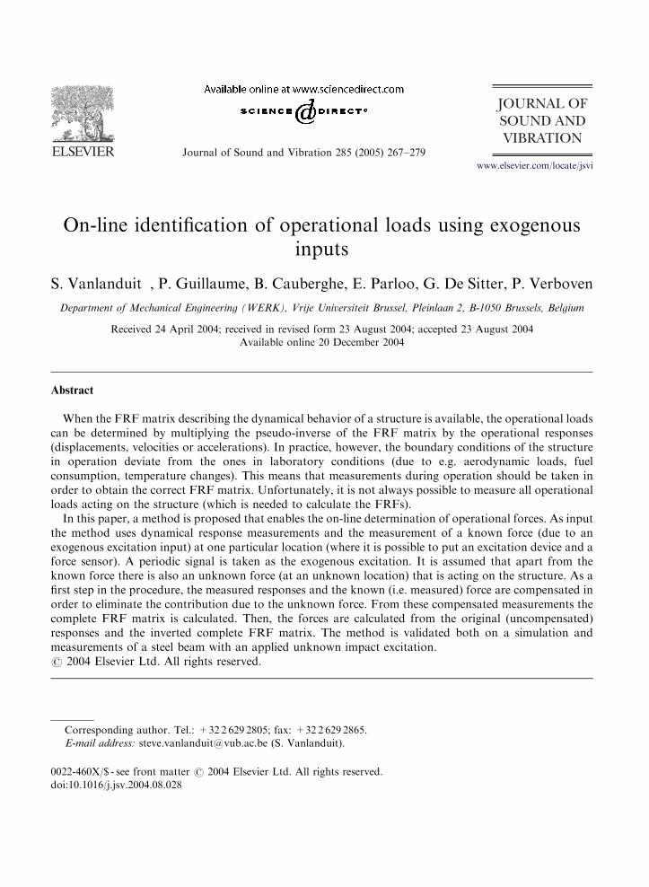
Fig. 5. Re-synthesized FRFs.

0 5 10 15 20-120

-100

-80

-60

-40

-20

Frequency, in Hertz

For

ce, i

n dB

(re

f 1N

)

Known force at even frequency lines: Fk(2nf0)

Unknown force: Fu(nf0)

Known force at odd frequency lines: Fk((2n+1)f0)

(a)

0 5 10 15 20-120

-100

-80

-60

-40

-20

Frequency, in Hertz

For

ce, i

n dB

(re

f 1N

)

Known force at even frequency lines: Fk(2nf0)

Unknown force: Fu(nf0)

Known force at odd frequency lines: Fk((2n+1)f0)

(b)

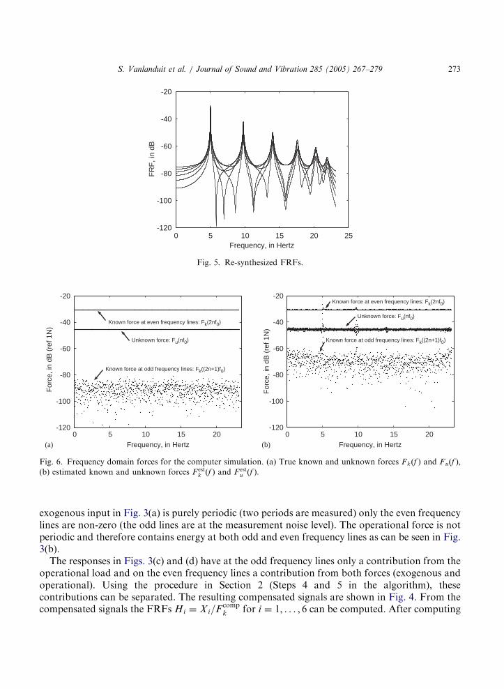
Fig. 6. Frequency domain forces for the computer simulation. (a) True known and unknown forces Fkðf Þ and Fuðf Þ;(b) estimated known and unknown forces F est

k ðf Þ and F estu ðf Þ:


exogenous input in Fig. 3(a) is purely periodic (two periods are measured) only the even frequencylines are non-zero (the odd lines are at the measurement noise level). The operational force is notperiodic and therefore contains energy at both odd and even frequency lines as can be seen in Fig.3(b).The responses in Figs. 3(c) and (d) have at the odd frequency lines only a contribution from the

operational load and on the even frequency lines a contribution from both forces (exogenous andoperational). Using the procedure in Section 2 (Steps 4 and 5 in the algorithm), thesecontributions can be separated. The resulting compensated signals are shown in Fig. 4. From thecompensated signals the FRFs Hi ¼ X i=F

compk for i ¼ 1; . . . ; 6 can be computed. After computing

ARTICLE IN PRESS

0 1 2 3 4 5-1

-0.5

0

0.5

1

Time, in seconds

For

ce, i

n N

(a)

3.5 4 4.5 5-2

0

2

4

6

8

10

Time, in seconds

For

ce, i

n N

(b)

Fig. 7. Time domain forces for the computer simulation. (a) Estimated known force f estk ðtÞ (full line) and difference

between true and estimated known force f estk ðtÞ � f kðtÞ (dotted line) Fkðf Þ; (b) estimated unknown force f est

u ðtÞ (full line)

and difference between true and estimated unknown force f estu ðtÞ � f uðtÞ (dotted line).


the modal parameters using the six FRFs a full modal model is obtained and the full FRF matrixcan be re-synthesized (six re-synthesized FRFs are shown in Fig. 5).By calculating the weighted inverse of the FRF matrix and multiplying these inverse FRFs with

the responses, the forces are estimated. The results—compared with the true values of theunmeasured forces—are shown in Fig. 6. Globally, there is about 1 dB error on the amplitude ofthe estimated unknown force. This is quite good keeping in mind that the inverse forceidentification problem has a bad numerical condition. Near the resonances of the structure up to10 dB error is obtained (this is due to the interpolation error in the compensation step of themethod). When comparing the true and estimated forces in the time domain (see Fig. 7) it can beseen that only a few percent error is made.

4. Experimental results

The experimental validation is performed on a beam which is freely supported. As theoperational load, an impact was generated with a calibrated hammer. The exogenous input (amulti-sine with random phases and uniform amplitudes) was applied with a B&K mini shaker andthe acceleration responses are measured at six locations with PCB accelerometers (the setup isshown in Fig. 8).Time domain and frequency domain measurements are shown in Figs. 9 and 10, respectively.

Again, the separation between the odd contribution (operational load only) and the evenfrequency lines (combination of exogenous and operational contribution) is clear.The compensated responses in Fig. 11 are much clearer (no distortions due to the unknown

operational pulsed force). These responses together with the compensated exogenous load areused to compute the complete modal model and the complete FRFs (see Fig. 12).

ARTICLE IN PRESS

0 0.5 1 1.5 2-10

-5

0

5

10

Time, in seconds

For

ce, i

n N

(a)

0 0.5 1 1.5 2

-20

-10

0

10

20

30

40

50

60

Time, in seconds

For

ce, i

n N

(b)

0 0.5 1 1.5 2

-10

-5

0

5

10

Time, in seconds

Acc

eler

atio

n, in

m/s

2

(c)

0 0.5 1 1.5 2

-10

-5

0

5

10

Time, in seconds

Acc

eler

atio

n, in

m/s

2

(d)

Fig. 9. Time data: (a) known force f kðtÞ; (b) unknown force f uðtÞ; (c) displacement at dof 1 x1ðtÞ; (d) displacement at

dof 6 x6ðtÞ:

Fig. 8. Measurement setup of the impulse identification experiment: (a) beam under test, (b) impact hammer for

application of unknown force f u; (c) shaker for application of known force f kðtÞ; (d) acceleration sensors at six

equidistant positions.


ARTICLE IN PRESS

0 200 400 600 800-70

-60

-50

-40

-30

-20

-10

0

Frequency, in Hertz

For

ce, i

n dB

(re

f 1N

)

Even frequency lines

Odd frequency lines

(a)

0 200 400 600 800-45

-40

-35

-30

-25

Frequency, in Hertz

For

ce, i

n dB

(re

f 1N

)

(b)

0 200 400 600 800-70

-60

-50

-40

-30

-20

-10

0

10

Frequency, in Hertz

Acc

eler

atio

n, in

dB

(re

f 1m

/s2 ) Even frequency lines

Odd frequency lines

(c)

0 200 400 600 800-70

-60

-50

-40

-30

-20

-10

0

10

Frequency, in Hertz

Acc

eler

atio

n, in

dB

(re

f 1m

/s2 ) Even frequency lines

Odd frequency lines

(d)

Fig. 10. Frequency domain data: (a) known force Fkðf Þ; (b) unknown force Fuðf Þ; (c) displacement at dof 1 X 1ðf Þ; (d)displacement at dof 6 X 6ðf Þ:


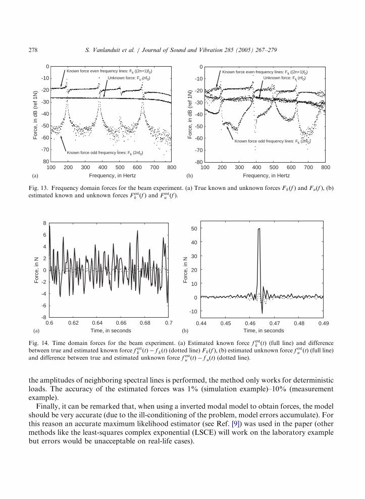
In the comparison of the spectra of the estimated forces (both known and unknown) with themeasured forces in Fig. 13, it can be seen that there is up to 10 dB of distortion on the estimatedload amplitudes. In the time domain, the estimated forces (both known f k and unknown f uðtÞ) hasan error of about 10% compared to the measured force (see Fig. 14). This is much better than onewould obtain without compensating for the unknown force in the calculation of the FRFs.

5. Conclusions

In this article a method was developed to estimated operational forces by using anexogenous periodic excitation signal. After compensating the response signals for thepresence of the operational load the complete FRF matrix is computed. The inverseof this FRF matrix is then used to calculate the loads. In addition to the unknown operationload, also the exogenous load is applied. This can then be used as a validation by comparingthe measured and estimated exogenous forces. Since in interpolation between the phases and

ARTICLE IN PRESS

0 200 400 600 800-70

-60

-50

-40

-30

-20

-10

0

Frequency, in Hertz

For

ce, i

n dB

(re

f 1N

)

(a)

0 200 400 600 800-70

-60

-50

-40

-30

-20

-10

0

10

Frequency, in Hertz

Acc

eler

atio

n, in

dB

(re

f 1m

/s2 )

(b)

0 200 400 600 800-70

-60

-50

-40

-30

-20

-10

0

10

Frequency, in Hertz

Acc

eler

atio

n, in

dB

(re

f 1m

/s2 )

(c)

Fig. 11. Compensated frequency domain data: (a) known force Fcompk ðf Þ; (b) displacement at dof 1 X

comp1 ðf Þ; (c)

displacement at dof 6 Xcomp6 ðf Þ:

0 200 400 600 800-80

-60

-40

-20

0

20

40

Frequency, in Hertz

FR

F, i

n dB

Fig. 12. Re-synthesized FRFs.


ARTICLE IN PRESS

100 200 300 400 500 600 700 800 80

-70

-60

-50

-40

-30

-20

-10

0

Frequency, in Hertz

For

ce, i

n dB

(re

f 1N

)

Known force even frequency lines: Fk ((2n+1)f0)

Known force odd frequency lines: Fk (2nf0)

Unknown force: Fu (nf0)

(a)

100 200 300 400 500 600 700 800-80

-70

-60

-50

-40

-30

-20

-10

0

Frequency, in Hertz

For

ce, i

n dB

(re

f 1N

)

Known force even frequency lines: Fk ((2n+1)f0)

Unknown force: Fk (nf0)

Known force odd frequency lines: Fk (2nf0)

(b)

Fig. 13. Frequency domain forces for the beam experiment. (a) True known and unknown forces Fkðf Þ and Fuðf Þ; (b)estimated known and unknown forces F est

k ðf Þ and F estu ðf Þ:

0.6 0.62 0.64 0.66 0.68 0.7-8

-6

-4

-2

0

2

4

6

8

Time, in seconds

For

ce, i

n N

(a)0.44 0.45 0.46 0.47 0.48 0.49

-10

0

10

20

30

40

50

Time, in seconds

For

ce, i

n N

(b)

Fig. 14. Time domain forces for the beam experiment. (a) Estimated known force f estk ðtÞ (full line) and difference

between true and estimated known force f estk ðtÞ � f kðtÞ (dotted line) Fkðf Þ; (b) estimated unknown force f est

u ðtÞ (full line)

and difference between true and estimated unknown force f estu ðtÞ � f uðtÞ (dotted line).


the amplitudes of neighboring spectral lines is performed, the method only works for deterministicloads. The accuracy of the estimated forces was 1% (simulation example)–10% (measurementexample).Finally, it can be remarked that, when using a inverted modal model to obtain forces, the model

should be very accurate (due to the ill-conditioning of the problem, model errors accumulate). Forthis reason an accurate maximum likelihood estimator (see Ref. [9]) was used in the paper (othermethods like the least-squares complex exponential (LSCE) will work on the laboratory examplebut errors would be unacceptable on real-life cases).

ARTICLE IN PRESS


Acknowledgements

This research has been sponsored by the Flemish Institute for the Improvement of the Scientificand Technological Research in Industry (IWT), the Fund for Scientific Research—Flanders(FWO) Belgium. The authors also acknowledge the Flemish government (GOA-Optimech) andthe research council of the Vrije Universiteit Brussel (OZR) for their funding. The first authorhold a grant as a Postdoctoral Researcher from the FWO Vlaanderen.

References

[1] K.K. Stevens, Force identification problems: an overview, in: Proceedings of the SEM Spring Meeting, Houston,

USA, 1987, pp. 838–844.

[2] M.T. Martin, J.F. Doyle, Impact force identification from wave propagation responses, International Journal of

Impact Engineering 18 (1996) 65–77.

[3] P. Guillaume, E. Parloo, G. De Sitter, Source identification from noisy response measurements using an iterative

weighted pseudo-inverse approach, in: Proceedings of ISMA2002, Leuven, Belgium, 2002, pp. 1817–1824.

[4] P. Guillaume, E. Parloo, P. Verboven, G. De Sitter, An inverse method for the identification of localized excitation

sources, in: Proceedings of the 20th International Modal Analysis Conference, Los Angeles, USA, 2002.

[5] W. Heylen, S. Lammens, P. Sas, Modal Analysis Theory and Testing, PMA, KU Leuven, 1998.

[6] E. Parloo, P. Verboven, P. Guillaume, M. Van Overmeire, Force identification by means of in-operation modal

models, Journal of Sound and Vibration 262 (2003) 161–173.

[7] I. Bruant, G. Coffignal, F. Lene, M. Verge, A methodology for determination of piezoelectric actuator and sensor

location on beam structures, Journal of Sound and Vibration 243 (5) (2001) 861–882.

[8] S. Vanlanduit, P. Guillaume, B. Cauberghe, Elimination of background disturbance from measurement spectra,

Measurement Science and Technology 14 (2003) 155–163.

[9] P. Guillaume, P. Verboven, S. Vanlanduit, Frequency-domain maximum likelihood identification of modal

parameters with confidence intervals, in: Proceedings of ISMA1998, Leuven, Belgium, 1998, pp. 359–366.

On-line identification of operational loads using exogenous inputs

Documents

Transcript of On-line identification of operational loads using exogenous inputs