The Influence of Land-use

Activities on Nutrient Inputs into Upland Catchment Streams, Ghana

Dissertation

zur

Erlangung des Doktorgrades (Dr. rer. nat)

der

Mathematisch-Naturwissenschaftlichen Fakultät

der

Rheinischen Friedrich-Wilhelms-Universität Bonn

vorgelegt von

ADELINA MARIA MENSAH

aus

GHANA

Bonn 2009

1. Referent: Prof. Dr. Paul Vlek 2. Referent: Prof. Dr. Sebastian Schmidtlein Tag der Promotion: 17.07.2009 Erscheinungsjahr: 2009 Diese Dissertation ist auf dem Hochschulschriftenserver der ULB Bonn http://hss.ulb.uni-bonn.de/diss_online elektronisch publiziert

Life is simple. Man complicates it when he doesn’t follow the simple pathways that govern. An honorable intension is the beginning; persistent questioning, the direction; and inner guidance, the key. Then man works with life to create magnificence.

- Adelina Mensah, July 17 2008 -

To my parents, for giving me the opportunity to create

ABSTRACT

In Ghana, increasing agricultural productivity is seen as an essential component of most development programs. The main objective of this study was to assess the implications of increased land-use activities on in-stream nutrients and impacts on the quality of water for domestic use and on aquatic ecosystem health. To guide the evaluation of the land-water interlinkages, the conceptual structure defined by the DPCER (Driving forces-Pressure-Chemical state-Ecological state-Response) framework was used, which is an adapted version of the traditional DPSIR (Driving forces-Pressure-State-Impact-Response) model. The study compares three small upland sub-catchments in the same geo-morphologic Ofin Basin of the Ahafo-Ano South District. Based on the percentage cover of natural land to agricultural land, the catchments were categorized as low (Nyamebekyere), medium (Dunyankwanta), and high (Attakrom) land-use intensities. With simple mathematical tools and selected indicators, the performance of each link within the DPCER framework was evaluated, and with the comparison of each set of indicators between catchments, changes as a function of land-use intensity were assessed.

Despite overall minimal fertilizer use in Ghana, there were significant differences between the sub-catchments regarding the proportion of farmers who applied fertilizers. Attakrom showed the highest numbers of farmers (20.5%) as compared to Dunyankwanta (12.3%) and Nyamebekyere (0.0%), with applications mainly to cash crops such as cocoa and maize. Simple logistic regression explained that fertilizer use was considerably influenced by the farmer’s access to services such as farm loans and agricultural extension services, in addition to property rights and residential status. The Beale’s Ratio method, used to calculate the total annual load (kg yr-1) and yield (kg ha-1) for major nutrients (Ca, K, Mg, Na, NO3-N, NH4-N, and PO4-P), showed that the highest nutrient export was from Dunyankwanta at a relative magnitude of up to 3-fold the values of the other two catchments. The annual water yield was highest in Dunyankwanta (79.91 mm yr-1) as compared to Nyamebekyere (41.33 mm yr-1) and Attakrom (22.87 mm yr-1). Total annual water yield was the main determinant of the total nutrient loads/yields, and ranged between 2.3% and 6.2% of the total annual precipitation. 48-hour grab water samples confirmed that in-stream nutrient concentrations increased with increasing land-use intensity, with significant differences between catchments for the major cations (Ca, Mg, K and Na). Median values for all nutrients were in the optimal range of the Ghana Target Water Quality Range (TWQR) for domestic use and for aquatic ecosystem health. The distribution of macroinvertebrate taxa as a function of stream chemistry also showed significant differences in the ecological states of the upland catchment streams.

The DPCER framework with a comparative catchment component was an effective methodology for describing changes as land-use intensifies. Water yield is important in estimating total nutrient export, and the inclusion of a hydrological component in the DPCER framework is proposed - to form a DHPCER model (Driving forces-Hydrology-Pressure-Chemical state-Ecological state-Response). The significant differences observed in each component of the framework strongly suggest anthropogenic influence. With Ghana’s objectives for increased agricultural productivity, the results of this study demonstrate the need for incorporating integrated water resource management into development agendas.

KURZFASSUNG

Die Auswirkungen der zunehmenden Landnutzung auf die Nährstoffe in den Flussaufwärtsläufen in Ghana In Ghana wird eine Steigerung der landwirtschaftlichen Produktivität als notwendiger Bestandteil der meisten Entwicklungsprogramme betrachtet. Das Hauptziel dieser Studie ist die Bewertung der Auswirkungen der zunehmenden Landnutzungsaktivitäten auf die Nährstoffe in den Wasserläufen sowie auf die Qualität des Wassers für den häuslichen Gebrauch und der Wasserökosysteme. Um die Ermittelung der Land-Wasser-Zusammenhänge zu unterstützen, wurde das DPCER-Modell (Driving forces-Pressure-Chemical state-Ecological state-Response) eingesetzt, eine überarbeitete Version des traditionellen DPSIR- Modells (Driving forces-Pressure-State-Impact-Response). Die Studie vergleicht drei kleine Wassereinzugsgebiete im Hochland im gleichen geo-morphologischen Becken im Ahafo-Ano South Distrikt. Auf der Grundlage des Anteils von Land mit natürlicher Vegetationsbedeckung im Vergleich zu landwirtschaftlichen Flächen wurden diese drei Bereiche klassifiziert als Gebiete mit niedriger (Nyamebekyere), mittlerer (Dunyankwanta) bzw. hoher (Attakrom) Landnutzungsintensität. Mit einfachen mathematischen tools und ausgewählten Indikatoren wurde die Leistung jeder Verknüpfung innerhalb des DPCER bewertet und die Veränderungen als Funktion von Landnutzungsintensität durch den Vergleich der einzelnen Indikatorgruppen der Einzugsgebiete bestimmt.

Trotz einem insgesamt geringen Verbrauch von Dünger in Ghana zeigen sich signifikante Unterschiede zwischen den drei Gebieten in Bezug auf den Anteil der Farmer, die Dünger benutzten. In Attakrom war die Anzahl der Farmer am höchsten (20.5%) verglichen mit Dunyankwanta (12.3%) und Nyamebekyere (0.0%), wobei der Dünger hauptsächlich beim Anbau von Cash Crops wie Kakao und Mais eingesetzt wurde. Die einfache logistische Regression deutet daraufhin, dass der Gebrauch von Dünger stark durch den Zugang der Farmer zu, z.B., Krediten und landwirtschaftlicher Beratung beeinflusst wird sowie durch Landbesitzrechte und Wohnstatus. Die Beale’s Ratio-Methode, die für die Berechnung der jährlichen Gesamtmenge (kg Jahr-1) und Menge per Hektar (kg ha-1) der wichtigsten Nährstoffe (Ca, K, Mg, Na, NO3-N, NH4-N, and PO4-P) eingesetzt wurde, zeigt den höchsten Nährstoffexport aus Dunyankwanta mit einem relativen Wert von bis zu dreimal der Werte der anderen beiden Gebiete. Der jährliche Wasservolumen per Hektar war am höchsten in Dunyankwanta (79.91 mm Jahr-1) verglichen mit Nyamebekyere (41.33 mm Jahr-1) und Attakrom (22.87 mm Jahr-1). Dieser Wert war der Hauptfaktor bei der Bestimmung der Gesamtnährstoffe und lag zwischen 2.3% und 6.2% des jährlichen Niederschlags. Die Ergebnisse der 48-stündlichen Wasserproben (grab sampler) bestätigen, dass die Nährstoffkonzentrationen in den Wasserläufen mit der Landnutzungsintensität steigen mit signifikanten Unterschieden zwischen den Einzugsgebieten bei den wichtigsten Kationen (Ca, Mg, K und Na). Die mittleren Werte für alle Nährstoffe waren im optimalen Bereich der Ghana Target Water Quality Range (TWQR - Qualitätsgrenzwerte) für Haushaltswasser und Wasserökosysteme. Die Verteilung der Taxa der Makrowirbellosen, die von den chemischen Zusammensetzungen der Flüsse beeinflusst ist, zeigte signifikante Unterschiede im ökologischen Zustand der Einzugsgebiete im Hochland.

Das DPCER Modell mit einer Komponente zum Vergleich der Einzugsgebiete ist eine effektive Methode zur Beschreibung der Veränderungen als Folge von zunehmender Landnutzungsintensität. Der Wasservolumen per Hektar ist wichtig bei der Ermittlung des gesamten Nährstoffexports; die Einbeziehung einer hydrologischen Komponente im DPCER zur Bildung eines DHPCER Modells (Driving forces-Hydrology-Pressure-Chemical state-Ecological state-Response) wird vorgeschlagen. Die beobachteten signifikanten Unterschiede deuten stark auf menschlichen Einfluss hin. Ghana hat eine Steigerung der landwirtschaftlichen Produktivität zum Ziel und die Ergebnisse dieser Studie zeigen, dass es notwendig ist, integriertes Wassermanagement bei Entwicklungsprogrammen hierbei zu berücksichtigen.

TABLE OF CONTENTS

1 INTRODUCTION ........................................................................................... 1

1.1 Land-use and impacts to the aquatic ecosystem .............................................. 2 1.2 Conceptual framework and research objectives .............................................. 4 1.2.1 Research structure............................................................................................ 7 1.2.2 Research question and main objectives ........................................................... 9 1.3 Justification of the study ................................................................................ 10 1.4 Structural overview........................................................................................ 11

2 LITERATURE REVIEW .............................................................................. 13

2.1 Introduction ................................................................................................... 13 2.2 Landscape and river ecosystems .................................................................... 14 2.2.1 Integrated assessment .................................................................................... 15 2.3 Interlinkages - using the DPCER approach ................................................... 17 2.3.1 Driving forces - land-use and agriculture ...................................................... 20 2.3.2 Pressure - Nutrient loading ............................................................................ 26 2.3.3 Hydrology .................................................................................................. 27 2.3.4 Chemical state - Stream physico-chemistry .................................................. 37 2.3.5 Ecological state - Biotic fauna ....................................................................... 41 2.3.6 Policy response .............................................................................................. 46

3 STUDY AREA .............................................................................................. 49

3.1 General description ........................................................................................ 49 3.1.1 Climate .................................................................................................. 50 3.1.2 Physical features ............................................................................................ 51 3.1.3 Land use and agriculture ................................................................................ 52 3.1.4 Vegetation .................................................................................................. 53 3.1.5 Social Setting ................................................................................................. 53 3.2 Sample site description .................................................................................. 54 3.2.1 Upland Catchments........................................................................................ 56 3.2.2 Downstream Sites .......................................................................................... 58

4 LAND USE AND FARMING SYSTEMS ................................................... 65

4.1 Introduction ................................................................................................... 65 4.2 Methodology .................................................................................................. 66 4.2.1 Data analysis .................................................................................................. 68 4.3 Results and discussion ................................................................................... 68 4.3.1 Services .................................................................................................. 69 4.3.2 Household characteristics .............................................................................. 71 4.3.3 Wealth .................................................................................................. 78 4.3.4 Farming and cropping system........................................................................ 85 4.3.5 Water resources and sanitation ...................................................................... 98 4.4 Summary ...................................................................................................... 100

5 LAND USE AND STREAM NUTRIENTS ............................................... 102

5.1 Introduction ................................................................................................. 102 5.2 Methodology ................................................................................................ 103 5.2.1 Hydrology ................................................................................................ 103 5.2.2 Physico-chemistry and nutrient ion concentration ...................................... 104 5.3 Data Analysis ............................................................................................... 107 5.3.1 Hydrology ................................................................................................ 107 5.3.2 Stream chemistry ......................................................................................... 112 5.3.3 Nutrient load estimation .............................................................................. 113 5.3.4 Statistical tests ............................................................................................. 117 5.4 Results and Discussion ................................................................................ 119 5.4.1 Annual dynamics ......................................................................................... 119 5.4.2 Temporal dynamics ..................................................................................... 132 5.5 Summary ...................................................................................................... 144

6 AQUATIC MACROINVERTEBRATES AND STREAM PHYSICO-

CHEMISTRY .............................................................................................. 146

6.1 Introduction ................................................................................................. 146 6.2 Methodology ................................................................................................ 147 6.2.1 Watershed/Habitat Approach ...................................................................... 147 6.2.2 Physico-Chemical Condition ....................................................................... 147 6.2.3 Biological Condition ................................................................................... 148 6.2.4 Quality Assurance........................................................................................ 148 6.3 Data Analyses .............................................................................................. 149 6.3.1 Macroinvertebrate assemblage description ................................................. 149 6.3.2 Site grouping based on macroinvertebrate assemblages ............................. 151 6.3.3 Site grouping based on environmental variables ......................................... 151 6.3.4 Community structure and environmental variable linkages ........................ 151 6.3.5 Measurement of community stress .............................................................. 152 6.4 Results ......................................................................................................... 153 6.4.1 Macroinvertebrate assemblage .................................................................... 153 6.4.2 Site grouping based on macroinvertebrate assemblage ............................... 158 6.4.3 Site groupings based on environmental variables ....................................... 161 6.4.4 Linking environmental factors to macroinvertebrate assemblage structure ................................................................................................ 170 6.4.5 Measurement of community stress .............................................................. 173 6.5 Discussion .................................................................................................... 175 6.6 Summary ...................................................................................................... 181

7 DPCER SYNTHESIS .................................................................................. 182

7.1 Interlinkages ................................................................................................ 182 7.1.1 Drivers of land-use intensification .............................................................. 184 7.1.2 Pressure – nutrient loading .......................................................................... 186 7.1.3 Chemical state – physico-chemistry and nutrient ion concentrations ......... 192 7.1.4 Ecological state ............................................................................................ 196 7.2 Integrated research challenges ..................................................................... 198

8 CONCLUSIONS AND RECOMMENDATIONS ...................................... 200

8.1.1 Driving forces .............................................................................................. 200 8.1.2 Pressure – nutrient loads/yields ................................................................... 201 8.1.3 Chemical state.............................................................................................. 202 8.1.4 Ecological state ............................................................................................ 202

9 REFERENCES ............................................................................................ 203

10 APPENDICES ............................................................................................. 232

ACRONYMS

CSIR Council for Scientific and Industrial Research CWSA Community Water and Sanitation Agency DO Dissolved Oxygen DPCER Driving forces-Pressure-Chemical state-Ecological state-Response DPSIR Driving forces-Pressure-State-Impact-Response DSR Driving Force-State-Response EC European Commission EEA European Union Agency EPA Environmental Protection Agency EPT Enteromorpha Plecoptera Trichoptera ET0 Potential Evapotranspiration ETa Actual Evapotranspiration ETO Enteromorpha Trichoptera Odonata EU European Union FAO Food and Agriculture Organisation FPC Flood Pulse Concept GPRS Ghana Poverty Reduction Strategy GVP GLOWA-Volta Project IDA Irrigation Development Authority MA Millennium Assessment framework MCA Millennium Challenge Account OECD Organization for Economic Co-operation and Development PCA Principal Component Analysis PRIMER Plymouth Routines in Multivariate Ecological Research PSR Pressure-State-Response PURC Public Utilities Regulatory Commission RCC River Continuum Concept SEA Strategic Environmental Assessment TWQR Target Water Quality Range UNCSD United Nations Commission for Sustainable Development UNEP United Nations Environment Programme UNSD United Nations Statistics Division WFD Water Framework Directive WRC Water Resources Commission WRI Water Resources Institute

Introduction

1

1 INTRODUCTION

A critical environmental resource that forms the basis of ecosystem functioning and

human well-being is the availability and quality of freshwater (MA 2005a; UNEP

2006a). With global population growth and related increasing land-use activities, the

integrity of aquatic ecosystems has become compromised by point and non-point

sources of pollution. The latter is comparatively more difficult to quantify and control,

as input and its impacts are usually the combined effects of the type of land-use and the

biophysical processes that influence transport and in-stream dynamics of the pollutants.

In many developed countries, the interactions between human and biophysical factors

have been incorporated into integrated management policies to improve the sustainable

use of water. Scientific evaluations to assess, monitor, and advise policy makers are

guided by conceptual frameworks, e.g., the well known Pressure-State-Response (PSR)

structure developed by the Organization for Economic Co-operation and Development

(OECD) (OECD 1998), which eventually evolved into the Driving forces-Pressure-

State-Impact-Response (DPSIR) framework currently used by the European Union (EC

2003). These frameworks consist of sets of indicators that represent major elements in

the interlinkages of driving forces of land-use, the ecological state of the aquatic system,

and policy responses.

With escalating global fuel and food prices, Ghana is reinforcing development

strategies for increasing agricultural productivity, especially for rural smallholder

farmers (GNA, May 2008). The environmental implications of agricultural activities to

freshwater systems are currently not assessed, as water quality monitoring programs

have been limited to routine physico-chemical assessments and minimal integrated

evaluations of terrestrial sources of contribution. With downstream users depending

directly on rivers for their domestic water supply and the environmental/social

implications of increased nutrients to vulnerable freshwater/coastal/marine ecosystems,

there is the need for an integrated research approach to evaluate these interactions

across the human-environment spectrum. The overall objective of this study is,

therefore, to adapt the well-known DPSIR conceptual framework to evaluate the

interlinkages in small catchments in Ghana, between land-use intensification and

impacts on water quality for domestic use and on aquatic ecosystem health.

Introduction

2

1.1 Land-use and impacts to the aquatic ecosystem

According to the Human Development Report 2006 (UNDP 2006), water gives life to

everything and is essential to human development and freedom, and therefore crucial in

providing human security and attaining the Millennium Development Goals (MDGs).

Conversely, increased agriculture is a main negative influence on freshwater quality and

quantity (UNEP 2006b). Food security (i.e., availability, affordability, access) has been

identified as the key solution to poverty alleviation and economic development in sub-

Saharan Africa (General Assembly Resolution 55/2 2000; MA 2005a; World

Development Report 2008). In attempts to address this, considerable effort has been

devoted to strategies for increasing agricultural production in smallholder farming (i.e.,

access to loans, improved seed quality, access to agro-chemicals and technical advice),

as the local communities of the rural poor are highly dependent on subsistence farming

(World Bank 2008a). In Ghana, this effort promises a strong potential for poverty

reduction, as agriculture accounts for 60% of employment and 37.2% (in 2006) of the

GDP (CIA 2008; World Bank 2008b). Various national programmes such as the revised

Ghana Poverty Reduction Strategy (GPRS II), the Food and Agriculture Sector

Development Plan, and internationally supported grants such as the $500 million US-

supported Millennium Challenge Account (MCA) have been launched to ensure

increased agricultural production and productivity of high value cash and food crops in

Ghana. More recently (effective from July 4, 2008), this has included the subsidization

of fertilizers, with prices reduced by 40-50% for poor small holder farmers.

The land-use and land-cover changes (LUCC) that accompany the conversion

of natural lands to agricultural production reduce vegetative cover and deteriorate soil

properties, thus invariably altering hydrological patterns and increasing the potential for

runoff and erosion (DeFries and Eshleman 2004). The increased application of

fertilizers and pesticides to improve productivity per unit area, in addition to inputs from

livestock manure, accumulates nutrient content in soils. Depending on the physical

location, chemical speciation, fate and environmental availability of the agrochemicals

in the soil, they are transported via surface runoff and other hydrological routes and

contribute to pollution of surface water bodies. With significant nutrient enrichment in

the streams during rainfall, the more sensitive taxa within the aquatic community

structure are affected such that the natural balance in community dynamics and

Introduction

3

ecosystem functioning is modified to affect productivity and biodiversity (Rabalais

2002). Services provided by the freshwater ecosystem such as water for human

consumption, nutrient cycling and retention, water filtering, water storage and aquifer

recharge, shoreline protection and erosion control, and a range of food and material

products (fish, shellfish, timber and fiber), are therefore affected (MA 2005a). The

cumulative impacts downstream affect the very productive but fragile coastal wetlands

and marine systems and result in reduced biodiversity, reduced numbers in

economically valuable species, algal blooms, increased sedimentation, and reduced

ecosystem health (Anderson et al. 2002; Seitzinger and Harrison 2005). Significant

amounts of fertilizer have been released into the environment in the past century,

impacting freshwater systems, estuaries and semi-enclosed and enclosed seas (IMBER

2005). Projected increases over the next three decades has suggested a 10-20% global

increase in river nitrogen flows to coastal ecosystems, continuing the trend of an

increase of 29% between 1970 and 1995 (MA 2005a).

In addition to environmental factors, e.g., climate, soil, and hydrogeology, that

affect the transport of nutrients into the aquatic systems, there are also cultural and

socioeconomic influences which explain how and why farmers relate to the soil (e.g.,

intensity and patterns of cropping and tillage). In sub-Saharan Africa, land tenure

arrangements which are not well established and the practice of shifting cultivation can

influence a farmer’s indifference to loss of future economic returns to the land, since

they are not directly affected by the declining land productivity associated with nutrient

mining (Henao and Baanante 2006). Farmers under pressure to engage in the market

may abandon more environmentally friendly practices to produce improved crops

(UNEP 2006b). The Millennium Assessment framework (MA 2005b) illustrates how

the changes in drivers that indirectly affect biodiversity (such as population, market,

governance, technology, lifestyle, etc.) can lead to changes that directly affect

biodiversity (e.g., change in land use, species introduction, technology adaptations,

harvest and resource consumption), which result in changes to ecosystem services that

eventually influence human wellbeing.

Although sub-Saharan Africa is reported to use less than 10% of the world’s

average in fertilizers, i.e., 8 kg ha-1 compared to 100 kg ha-1 worldwide (Henao and

Baanante 2006; Kelly 2006; UNEP 2006b), higher food productivity is being advocated

Introduction

4

for by increasing agro-chemical use. Increasing disposable income, in addition to

growing commercialization and the focus of development agencies on improving yields

of small farmers, is likely to increase the demand for chemical products (UNEP 2006b).

Concerns about the severity of soil degradation and soil nutrient depletion for African

grasslands suggests the need for careful management in strategies for optimizing

productivity (Bationo et al. 1998; Drechsel et al. 2001; Vlek 2005). With the potential

range of negative environmental impacts on soil and water quality, exacerbated by

inappropriate fertilization and irrigation practices, improving the resource base, i.e., soil,

in order to increase productivity in a way which conserves the natural resource and

prevents further degradation is a serious challenge. Trends already show an increase in

the concentration of nitrates and phosphates at river mouths in Africa, mirroring trends

observed in southeast Asia (UNEP 2002).

1.2 Conceptual framework and research objectives

The conceptual framework for this research, i.e., the organizational structure with sets

of indicators that represent the various elements that interact with each other, places the

environment as its central focus, although acknowledging the equal importance of

societal wellbeing. The Driving forces-Pressure-State-Impact-Response (DPSIR)

concept, developed for environmental reporting purposes by the European Commission

(EC 2000, 2003), provides a general framework for organizing information about an

environmental issue by formalizing the relationship between various sectors of human

activity and the environment. An environmental indicator developed under the DPSIR

model can be categorized as a driving force, pressure, state, impact or response

indicator, according to the type of information it provides. Together, these indicators

demonstrate how people’s activities and environmental effects are interconnected, and

the effectiveness of policy and management responses to environmental issues. The

framework elaborates the cause-effect relationships between interacting components of

complex social, economic and environmental systems and has been widely applied

internationally.

For this study, the conceptual definitions for each link within the framework is

based on adaptations provided by the Driving forces-Pressure-Chemical state-

Ecological state-Response (DPCER) method (Rekolainen et al. 2003). According to the

Introduction

5

authors, the change from ‘state’ (S) and ‘impact’ (I) to ‘chemical state’ (C) and

‘ecological impact’ (E) was justified by the fact that surface water status has been

defined by chemical quality elements and ecological quality indicators by the European

Union Water Framework Directives (WFD).

The DPCER framework assumes that there is a dynamic interaction between

land-use activities and aquatic ecosystem functions. In the absence of established risks

and obvious policies that have been taken to improve the chemical or ecological status

of the studied streams, the response component (R) is not assessed. The adaptation of

the DPCER model, therefore, is unidirectional for this study, i.e., begins with assessing

the driving forces in agricultural activities that lead to an observed ecological state. At

each level in the framework, the following specific parameters are defined;

• Driving forces of change are underlying factors that influence the intensity of land-

use (in this case, agriculture) in each of the catchments. In this study, agrochemical

use, for example, can also be influenced by socio-economic parameters such as

education or access to market.

• Pressure is represented by the measurement of the variables which directly lead to

environmental problems. For this study, this is assessed by quantitative estimates of

nutrient loads, measured in kg yr-1, and nutrient yields (kg ha-1) into streams.

• Chemical state is described by indicators which reveal the condition of the

environment, i.e., the stream physico-chemistry and nutrient ion concentration is

affected by nutrient loads and greatly influences biological and ecological

functioning of the system.

• Ecological state is assessed by indicators that represent the ecological effects of the

changes in the chemical state. For this study, community dynamics of

macroinvertebrates are assessed.

There are simple to complex models available to calculate, simulate and

account for various elements within the DPCER framework and their interactions,

depending on the needs of the research (Rekolainen et al. 2003). However, due to the

unavailability of data on hydrological and biophysical processes linking the terrestrial

and aquatic habitats for the studied catchments, the relatively short research period as

Introduction

6

compared to required timelines for effective modeling, and the logistical limitations of

detailed assessments of these processes based on the scope of this research, each of the

elements within the framework are evaluated by simple indicators. The choice of

indicators for each link and the mathematical tools for assessment are discussed,

including the uncertainties inherent in the individual fields and assumptions about

cause-effects in each sub-set of the linkages.

The study was carried out in three small inland valley catchments

(approximately 5 km2 each): (i) Nyamebekyere, a natural forested reserve, (ii)

Dunyankwanta, a moderately cultivated catchment area, and (iii) Attakrom, an

intensively cultivated area, based on classification by the VINVAL project (Meijerink et

al. 2003). These catchments are located in the same agro-ecological basin and share

similar geo-morphological characteristics except for their degree of land-use intensity,

an attribute that is assumed to minimize the natural environmental variations that may

occur. This scenario establishes major factors (based on literature review) that influence

agricultural activities as the main Driving forces (D) and contribute to the input of

nutrients in the streams, represented by Pressure (P) in the framework. Due to the

similarities of the catchments, and lack of information on the hydrological pathways of

nutrients from these soils to the streams, it is assumed that the estimates of total nutrient

loads (P) in the catchment streams are representative of the dilutions of terrestrial

nutrients, via surface runoff, into the streams. The catchment streams are all upland,

ephemeral, and flow only during the rainy season, and in-stream observations are

assumed to be influenced predominantly by land-use intensity and nutrient loads. With

consideration to the financial budget of the research, analyzed nutrients within the

streams (Chemical state, C) were specifically limited to compounds linked to fertilizer

application (nitrogen compounds and orthophosphates) and soil quality (major cations

calcium, magnesium, potassium and sodium). Given the high diversity of aquatic fauna,

macroinvertebrates have been the most widely researched as indicators of aquatic

ecosystem health, and there is a large database on general characteristics, albeit mostly

for temperate taxa. However, with the general standards established for representative

taxa, this research assesses the dynamics of the macroinvertebrate community structure

to reflect the state of the aquatic system (Ecological state, E).

Introduction

7

1.2.1 Research structure

Based on the conceptual framework described above, specific parameters were

measured in order to quantify each of the major components. As there are no standard

indicator sets for specific environmental issues, the selection of indicators was based on

the clearly outlined DPCER framework, with each indicator having a particular function

in the analytical problem solving the logic of the issue (Niemeijer and de Groot 2008a).

A diagrammatic representation of the indicators used for each link within the DPCER

conceptual framework is shown in Figure 1.1. For each element of the framework, the

indicator, method and specific objectives are presented below.

Overall, the research initially assesses specific measures within each of the

component disciplines involved within the framework, compares them to assess whether

there are relevant differences in the nutrient load/chemistry/ecology of streams in

upland catchments of varying degrees of land-use, and finally discusses possible factors

that may contribute to these differences.

DPCER framework

Driving forces Land-use intensity (agriculture)

Indicator Household characteristics and wealth, farming methods, land-use,

water use

Methods Structured questionnaire

• Describe socio-economic factors associated with land-use and agricultural activities

within each catchment at household level

• Statistically determine the significant differences between catchments.

Pressure Total nutrient load/yield in each catchment stream

Indicator Nutrient loads/yields of Ca, K, Mg, Na, NH4-N, NO3-N

and PO4-P

Methods Hydrology, nutrient ion concentration and stream flow data

• Establish basic hydrology for each upland catchment stream.

• Estimate total load (kg yr-1) and yield (kg ha-1) of nutrients transported out of each

of the upland catchment streams in defined periods (monthly, seasonally, and

annually).

• Compare nutrient yields between the catchments.

Introduction

8

Chemical state Temporal dynamics in stream physico-chemistry

Indicator Dissolved oxygen, electro-conductivity, pH and temperature.

Concentrations of Ca, K, Mg, Na, NH4-N, NO3-N and PO4-P

Methods Hydrology, physico-chemistry, nutrient ion concentration

• Establish temporal patterns in flow-weighted concentrations (mg L-1) of ionic

components of the stream.

• Compare stream physico-chemistry and nutrient ion concentrations to Ghana’s

Target Water Quality Ranges (TWQRs) established for domestic use and aquatic

ecosystem health for freshwater

• Assess relevant differences in concentrations between the catchments.

Ecological state Distribution of biotic communities in response to abiotic

parameters

Indicator Community structure of macroinvertebrates

Methods Periodic sampling of macroinvertebrates

• Assess the degree of site similarity or differences based on biotic composition and

the distribution of abiotic variables for the upland catchments.

• Link the patterns of observed taxa distribution to the differences in abiotic

parameters, and identify the specific abiotic variables that may be significant.

• Describe the macroinvertebrate community patterns and occurrences within and

between similarly grouped sites and examine the inter-relationship and contribution

of the observed taxa.

To conclude, the DPCER synthesis discusses significant factors in the application of the

conceptual framework, in order to evaluate interlinkages between land-use, nutrient

concentration and macroinvertebrate distribution in small upland catchments in Ghana.

This study contributes to the existing agro-economical information base

created by the VINVAL project. The 5-year project funded by the EU (2000-2005)

compared the same three catchments (in addition to a similar setup in Burkina Faso) to

examine how various degrees of land-use influence agricultural productivity and impact

terrestrial ecological functions. The effects of the observed changes in land-

Introduction

9

use/agricultural management and ecological functions were to be used to develop tools

for integrated land-use planning on the catchment level (yet unpublished). These tools

are mainly TechnoGIN, a technical coefficient generator, OSARIS, a GIS-based

knowledge system, and VINVAL Land Use Viewer, a community mapping method and

sociological tool for supporting participatory land-use planning (Verzandvoort et al.

2005). The analysis of the impact of different land-use development scenarios on the

ecological and production functions are to be supported by these tools in village

participatory land use planning workshops, where the decision-making process of land

development is carried out.

The research also contributes to the Analysis of Long-Term Environmental

Change component of the overall objectives of the Global Change in Hydrological

Cycle (GLOWA) Volta Project (GVP) that this study forms part of. The GVP assesses

sustainable water use under changing land-use patterns, rainfall reliability and water

demand in the Volta Basin by analyzing the physical and socio-economic determinants

of the basin’s hydrological cycle. The Volta Lake is the largest man-made lake (45% of

Ghana’s total surface area) created to generate hydropower, and has been the focus of

large-scale research on the socio-economic implications of ecosystem changes.

1.2.2 Research question and main objectives

The main research question of this study is “What is the influence of increasing land-use

activity on nutrient inputs into small upland catchment streams in Ghana?” The DPCER

framework provides a conceptual guideline to evaluate each of the contributory

components that describe the cause-effect interlinkage from land to stream. The general

objective of the study is to assess the extent of increasing land-use activity (mainly

agriculture) on in-stream nutrient inputs, and the impacts on water quality for domestic

use and on aquatic ecosystem health for upland catchments. Specifically, the objectives

are to:

• Describe the major socio-economic factors, or driving forces (D), that contribute

significantly to land-use intensity and the farming systems observed in the three

upland catchments.

Introduction

10

• Estimate the total in-stream nutrient loads and yields, which represent the land-use

pressure (P) that directly impacts the stream ecosystem.

• Evaluate the specific physico-chemical parameters and nutrient ion concentrations

(Ca, K, Mg, Na, NH4-N, NO3-N, and PO4-P) that describe the chemical state (C) of

each stream, and assess the differences between catchments.

• Examine macroinvertebrate taxa distribution as a function of the chemical state of

each catchment stream, in order to establish the ecological state (E).

• Explain the interlinkages between different components of the conceptual model as

land-use intensity increases, and assess the efficacy of the DPCER framework in

illustrating these changes.

1.3 Justification of the study

The fundamental concepts in the cause-effect chain described by the DPSIR framework

(EEA 1999; EC 2003) have been used effectively for a variety of environmental

systems to assess the interaction between drivers of land-use and the environmental

consequences in order to propose and monitor appropriate policies. In Ghana, there is a

lack of integrated research on agricultural activities and its impacts on freshwater

systems. Related issues have been mainly disciplinary, since establishing patterns of the

interacting elements between the different study fields requires extensive data to

incorporate processes such as nutrient export, hydrology, transport and fate of nutrients,

toxicology of aquatic biota, etc. To circumvent these limitations, this study proposes

and tests an adapted version of the traditional DPSIR framework, using the DPCER

conceptual definitions, and includes a comparative catchment component. With the

framework as a guideline, selected indicators representing links in the land-water

interaction are assessed for three small catchments in the same geo-morphologic basin

with varying degrees of land-use intensity, i.e., from natural or low intensity to mainly

agricultural or high land-use intensity. As the catchments are located in the same basin,

the comparative approach assumes that the influence of climatic and biophysical factors

on nutrient export and aquatic ecosystem dynamics are similar. The small upland

catchments provide an ideal platform for investigating agricultural impacts on nutrient

export, as the response time of the streams is shorter than for larger systems. In addition,

social assessments on a smaller scale contribute more information on the internal

Introduction

11

household factors that influence agricultural activities in Ghana. The framework enables

the assessment of how specific indicators perform in each catchment, and compares the

behavior between catchments to evaluate interlinkages as a function of land-use

intensity.

1.4 Structural overview

The thesis is divided into eight chapters. Chapter 1 introduces the research objectives

and the need for integrated research to evaluate the interlinkages between development

objectives of society, land-use and aquatic ecosystem health. The research structure is

presented based on the traditional DPSIR conceptual framework. Chapter 2 presents the

theoretical background of the interdisciplinary focus of research in land-use and the

aquatic ecosystem with references to fundamental theories and assessment

methodologies in the various disciplines covered in the study, i.e., agriculture,

hydrology, nutrient loading, physico-chemistry, and macroinvertebrates as

bioindicators. Chapter 3 describes the study area in Ghana and presents a more detailed

account of the sampled sites and associated catchment areas. Chapter 4 presents the

results and discussion of administered questionnaires on community characteristics and

farming practices, with focus on influencing socio-economic parameters on the

households in the catchments, as well as their farming/cropping systems and water

resource use. Chapter 5 describes the field, laboratory and statistical methods used to

determine water yield, assess physico-chemical dynamics and estimate nutrient

load/yield, with the results discussed. Chapter 6 presents a description of the

investigations undertaken for sampling of macroinvertebrate communities, with results

and discussions of the linkages between the observed community patterns and stream

physico-chemistry/nutrient ion concentrations. Chapter 7 addresses the over-arching

issue of the study and discusses the interlinkages between the three different disciplines

covered independently in Chapters 4, 5 and 6, in addition to the challenges of integrated

research. Chapter 8 summarizes key points and new observations of the research, with

recommendations for significant issues.

Introduction

12

Figure 1.1 Adapted DPCER framework (shaded box - major factors investigated; dotted box - assessed or estimated

variable)

Literature Review

13

2 LITERATURE REVIEW

2.1 Introduction

Land as an asset is used as a means to sustain livelihoods with activities based on needs or

underlying driving forces which affect production and consumption – e.g., property rights,

population density, development, available technology, pricing policies, among others. In

explaining the linkages between humans and their environments, most theorists agree that

human pressure on the environment is a product of three factors, population, affluence and

technology (Ehrlich and Ehrlich 1990). The impact of these factors are depicted in the

IPAT formula, where Impact (I) is the product of population (P), affluence (A) or

consumption per capita, and technology (T), which determines how many resources are

used and how much waste or pollution is produced for each unit of consumption. This

relationship, however assumes that the factors are independent of each other and excludes

interactions such as the improvement of technology when affluence increases or the

influence of culture and institutions. Classical theories such as neo-Malthusianism state that

human populations will increase exponentially to exceed the earth’s capacity for resource

renewal and lead to ecological consequences, whilst other theories have suggested that

population growth provides increased labor and capital inputs (Boserupian) as well as

improved human ingenuity and market substitution to avert future resource crises

(Cornucopian). For others, neither theory is totally accurate, as they may all operate at the

same time but under different regional or national economies (de Sherbinin et al. 2007).

The authors believe that inspite of this, continued discussions of interlinkages can lead to

improved policies on important issue areas including agricultural land degradation, water

resource management, and climate change.

Earlier research needing a quantifiable approach to analyze the interactions

between man and the environment focused mostly on population dynamics (size and

growth); however, the importance of other variables such as age, gender, household

demographics and the elements maintaining population equilibrium (fertility, mortality and

migration) have also been realized (McCusker and Carr 2006; de Sherbinin et al. 2008).

More recently, the influence of other interacting non-quantitative factors such as

Literature Review

14

institutions, policies, markets and cultural change are being incorporated (Lambin et al.

2001), with models such as the PEDA (Population, Environment, Development, and

Agriculture) integrating factors such as population, education, rural development, land

degradation, water, food production and food distribution for more effective

communication of these interactions to policy makers (Lutz et al. 2000). The cross-scale

dynamics of social-ecological systems (SESs) has also been described by the Panarchy

Theory (Gunderson et al. 1995) to explain the importance of adaptive evolution by both

systems and the multiple connections between different levels of organization and scales

(Walker et al. 2006). According to the theory, natural systems are linked together in

adaptive cycles of growth, accumulation, restructuring, and renewal. Changes can be

categorized into (i) gradual change, where human responses to ecological changes do not

involve a regime shift, (ii) adaptive change, to describe the ability of social components to

respond to shifts in ecological regimes, and (iii) transformative shifts, where both social

and ecological components transform into new regimes (Gunderson et al. 2006). Currently,

the understanding of the huge number of potential variables suggests the establishment of a

multilevel framework for SESs, where theories are tested as a subset when addressing a

particular issue (Ostrom 2008). Although considering all variables in addressing a specific

problem is close to impossible, users of the SES framework should bear in mind that causal

interactions between factors occur within the investigated system as well with progressive

upwards and downwards layers to larger or smaller systems.

2.2 Landscape and river ecosystems

Landscape ecology, which involves the interactions between aspects of geography, ecology

and social anthropology, considers humans as a significant component of the landscape,

and their perceptions and actions determine its relevance. From this viewpoint, the river is

another element of the landscape that is useful (e.g., for transportation, water sources, waste

disposal) or functional (e.g., exchange of materials, organisms, energy). From the

environmentalists point of view, the river is a dynamic entity of its own with spatial

linkages and processes related to its longitudinal (upstream to downstream), lateral (channel

bank and floodplain) and vertical (atmospheric, stream channel and subsurface) dimensions

Literature Review

15

(Vannote et al. 1980; Junk et al. 1989; Ward and Stanford 1989), with land use activities

influencing the ecological integrity and impacting habitat, water quality, and biota through

a variety of complex pathways (Johnson et al. 1997; Strayer et al. 2003; Turner and

Rabalais 2003; Zampella et al. 2007). With the consideration of river ecosystems as

‘riverscapes’ closely connected with the catchment landscape (Fausch et al. 2002; Wiens

2002), new methodologies for land-use studies are being required, especially when

necessary for the formulation of land-use policies (Rosegrant and Cline 2003). Sustainable

options for development require knowledge and skills from the biophysical system

dynamics, the multiple positions, perceptions, values, beliefs and interests of relevant

stakeholders, and the decisions required to apply simulated linkages to reality (van Paassen

et al. 2007).

2.2.1 Integrated assessment

The concept of connectivity and integration of biophysical, social and economic factors for

efficient environmental monitoring and management schemes requires an explicit structure

of the essential components and their interactions for the appropriate measures to be taken.

The system theory, defined as the description of a complex situation that is composed of a

number of elements and interactions within a specified boundary, provided a method for

conceptualizing the interactions between subsystems found in a society and the aquatic

environment in Bossel’s systemic framework (Bossel 1999, 2001). These interactions were

expanded to include the bi-directional interactions between the drivers that act on the

environment, the changes that as a consequence take place in the environment, and the

societal reaction to those changes. This forms the basis of three main water quality

conceptual frameworks: the pressure-state-response (PSR) typically used by the

Organization for Economic Co-operation and Development (OECD), driving forces-state-

response (DSR) used by the UN Commission on Sustainable Development, and the driving

forces-pressure-state-impact-response (DPSIR) used by the European Union Agency (EEA)

and European institutions (OECD 1998, 1999; Smeets and Weterings 1999; EEA 2000;

Washer 2000; OECD 2001). In comparison, frameworks such as the Millennium

Assessment (MA) is of a different ethical focus and concerned with the interaction of

Literature Review

16

indirect and direct drivers that affect ecosystem services for human wellbeing and poverty

reduction. Depending on the context of the issue, therefore, different frameworks offer

different possibilities for interpreting and integrating data into various conclusions and

policy recommendations – for example, the MA framework concentrates on sustainability

science and the DPSIR’s circular approach tends towards learning oriented management

thinking (Stoll-Kleeman et al. 2006).

Frameworks have various limitations, and the DPSIR and related frameworks

have been criticized for over-simplifying reality, ignoring other linkages within the socio-

ecological system, not incorporating the relations between the elements where responses to

one pressure can become pressure on another part of the system, and not addressing the fact

that some elements may be more relevant than others (Berger and Hodge 1998; Rekolainen

et al. 2003). Other comments suggest that the DPSIR has shortcomings in its function as a

neutral tool and is biased because it was designed to establish proper communication

between researchers and stakeholders/policy makers; and as such there is the need to

research into effective incorporation of the social and economic concerns of all

stakeholders (Svarstad et al. 2008). Due to these criticisms, parameters have to be based on

appropriate definitions, for example, definitions of driver and pressure given by the Water

Framework Directive (WFD) Guidance (EC 2003), before being applied to a specific issue

such as pressures from agricultural land use and impacts on surface water and groundwater

(Giupponi and Vladimirova 2006). In other cases, the framework can be further developed

to suit implementation processes, such as the DPCER (driving forces-pressure-chemical

state-ecological state-response) framework designed for the implementation of the WFD

(Rekolainen et al. 2003).

To qualitatively describe the dynamics within a framework, the representative

aspects are defined and characterized by selected parameters that can be measured.

Environmental indicators, known as key evaluators of the pressures, state, and response to

the environment, are now commonly used in environmental assessments to influence

management and policy making at different scales. An indicator is defined as a parameter

or a value that points to, provides information about, or describes the state of a

phenomenon/environment/area with a significance extending beyond that directly

Literature Review

17

associated with its value, and relays a complex message from numerous sources in a

simplified and useful manner (OECD 2003). Based on the conceptual framework, a

different rationale is used in the selection of indicators, thus the need to define the

context/purpose for monitoring such that the appropriate parameters are investigated.

Although indicators have been found useful, there have been some concerns that selected

indicators fail to capture the full complexity of the ecological system (Dale and Beyeler

2001; Bockstaller and Girardin 2003) and, more recently, the need to incorporate an

indicator’s analytical use or interaction within a set of selected indicators (Niemeijer and

De Groot 2008b). In an extensive list of common criteria for effective indicators, there is

very little mention of the inter-relation of indicators (i.e., integrative, linkable to societal

dimension and links with management), with the most common criteria being

measurability, low resource demand, analytical soundness, policy relevance and sensitivity

to changes within policy time frames (Niemeijer and De Groot 2008a). To incorporate the

real complexities, the interacting and interconnecting multiple causal chains were included

by the authors in a systematic indicator selection procedure known as the enhanced-DPSIR

framework (eDPSIR).

As the priorities of environmental policies have evolved, the need for more

reliable, synchronized and easily understandable information has also grown. Various

international and national programmes have established standardized criteria/guidelines or

sets of indicators to enable the exchange of experiences for strengthening environmental

monitoring and assessment – UN Statistics Division (UNSD), UN Environment Programme

(UNEP), UN Commission for Sustainable Development (UNCSD), European Union

(Commission of the European Communities, Eurostat, the European Environment Agency

– EEA) in addition to specialized agencies and non-governmental agencies (NGOs) – with

collaboration in order to build up synergies and avoid duplication of efforts in data

collection.

2.3 Interlinkages - using the DPCER approach

Accurate predictions of the impacts that landscapes have on stream ecosystems are

complicated by the complex interactions between natural and anthropogenic processes, the

Literature Review

18

influence of scale on responses, the uncertainties of long-term consequences after the

source of a disturbance is removed, and the fact that the magnitude of impact is not always

directly proportional to the pressure (Allan 2004). Different disturbances exert their

influence at different scales and by multiple pathways, which makes the matching of a

response to a specific stressor difficult. Natural variability makes these processes more

complex, and it is impossible to assess the degree of impairment accurately as there is less

certainty regarding the cause (Gergel et al. 2002; Thoms 2006). At various spatial scales,

the aquatic ecosystems are influenced by the prevailing characteristics, for example, stream

fauna is influenced by habitat quality, or the channel morphology by riparian vegetation

and supply of water and sediments. The appropriate temporal scales are also necessary

when delineating pressure and impact analysis, since some pressures may result in future

impacts, and some impacts may be related to past pressure no longer existent (EC 2003). In

addition, the response of stream conditions to a gradient of increasing land-cover change is

not always typical, due to the combined effects of separate responses of various parameters.

A study in West Africa, for example, showed no significant impacts on water yield and

river discharge when deforestation was below 50% of the forested area, overgrazing below

70% of savanna and 80% of grasslands (Li et al. 2007).

The use of indicators in the cause-effect linkage between components of the

agriculture-water quality interaction enables the description of the relationships between the

pressures caused by land-use activities and the impacts on the aquatic ecosystem. Although

criticized for its generic structure and bias, the clear definition of terms in the DPSIR

framework has enabled water resource researchers to identify appropriate indicators to

measure linkages within the framework. According to the WFD (EC 2003), driving forces

refers to an anthropogenic activity that may have an environmental effect, with economic,

social and demographic changes in the society being common indicators. With intensive

production and consumption, pressure is exerted that alter the use of the land and resources

to release substances or emissions. The state indicators describe the changes in quantity and

quality of the physical, chemical and biological characteristics of the environment. The

impact describes the environmental effect of the pressure (e.g., modified ecosystem), and

response, the measures taken to improve the state of the water body (e.g., policies to

Literature Review

19

develop best practices for agriculture). To improve the analytical utility of indicators, the

inter-relationship between selected indicators should be seen within a ‘causal chain

network’, where there are multiple interconnections and interactions between the links in

the framework instead of a single connection (Niemeijer and De Groot 2008a). Here, the

indicators are categorized as ‘root’, ‘central’ and ‘end-of-chain’ nodes, which describe the

source of problem to environmental impacts. This means that indicators are assessed

according to their function within the framework such that (i) those which provide

information on the source of the issue, e.g., fertilizer and manure inputs from agricultural

practices, are associated with the ‘root’ node, (ii) those interlinking indicators which assess

the impact of multiple processes occurring at the same time form the ‘central’ nodes, and

(iii) indicators located at the end of the series of cause-effect chains are the ‘end-of-chain’

nodes. Typically, biological organisms reflect the state or end-of-chain nodes, as they

develop morphological, physiological and/or life-history traits that minimize the impact of

disturbances over evolutionary time (Dίaz et al. 2008). The driving forces-pressure-

chemical state-ecological state-response model (DPCER), for example, is a modified form

of the DPSIR concept, which incorporates cause-consequence relationships and is policy

relevant for monitoring, assessing, and improving water quality resources (Rekolainen et

al., 2003). In this framework, driving forces refer to the specific land-use activities that lead

to the input of material (nutrients, sediments, toxins) (defined as pressures) to change the

chemical state of the environment (i.e., the physicochemical characteristics of the water

body) and result in changes to the ecological state (ecosystem modifications such as

changes in biota), with responses as societal measures to improve the state of the water

body. The assessment of the changes of the ‘state’ and the ‘impacts’ are the key indicators

used in selecting the appropriate ‘responses’ to influence the ‘driving forces’ or ‘pressure’

to the system.

The following sections discuss fundamental concepts for each of the links within

the DPCER framework. They include the assessment of the relationship between socio-

economic trends and land-use intensity, calculation of nutrient loading estimates,

accounting for physico-chemical processes, simulation of causal relationships between

Literature Review

20

chemical status and ecological status, and evaluation of environmental policies and

regulatory measures.

2.3.1 Driving forces - land-use and agriculture

Sustainable land-use has been defined as a unifying concept in which socio-economic

(production and consumption, economic efficiency and social equity) and agro-ecological

(resource stock, effect of land use on natural resources, etc.) variables coincide (Kruseman

et al. 1996). Land-use change is a complex process resulting from the interaction between

natural and social systems at different temporal and spatial scales (Fresco and Kroonenberg

1992; Lambin and Geist 2001; Veldkamp and Lambin 2001), with interactions between the

driving factors and impacts often referred to as feedback mechanisms (Claessens et al.

2008). This feedback of changes in land-use on human well-being, affects future land-use

decisions in a series of complex interactions and plays an important role in land-use studies

(Verburg 2006; Young et al. 2006).

To understand this complexity, a broad array of models and modeling methods are

available to researchers, with each type having certain advantages and disadvantages

depending on the objective of the research (Lambin et al. 2000; Veldkamp and Lambin

2001; Agarwal et al. 2002). In a detailed review of the functionality and ability of different

land-use models, the authors characterize three dimensions incorporated in land-use models

(space, time and human decision-making) and two distinct attributes for each dimension

(scale and complexity) (Agarwal et al. 2002). More recently, models such as the agent-

based models (ABMs) or multi-agent systems (MASs) (both are synonymous terms) are

more case specific, multi-scaled, multi-actor and data-intensive, and simulate the simple to

complex representations of the behavior and cognitive processes of the actors who make

land and resource use decisions (Robinson et al. 2007; Valbuena et al. 2008). In these

models, decision-making entities are represented by agents, and biophysical environment is

defined by spatial data. Five empirical approaches have been identified for obtaining

information on human and social actors, and include (i) sample surveys, (ii) participant

observation, (iii) field and laboratory experiments, (iv) companion modeling, and (v) GIS

Literature Review

21

and remotely sensed data, each of which has its inherent strengths and weaknesses

(Robinson et al. 2007).

Some authors have debunked myths that worldwide only population growth and

poverty are the major underlying causes of land-use change, but rather people’s responses

to economic opportunities, influenced by both local and national markets and policies

(Lambin et al. 2001). In developing countries, land-use dynamics are found within the

agricultural sector, which is the main source of livelihood (Lambin et al. 2000; Soini 2005;

McCusker and Carr 2006; World Bank 2008a). Individual farms, generally for the purpose

of producing food and meeting other household goals, vary due to unique conditions of

available resources and household circumstances, and function within an existing social,

economic and institutional environment (Dixon et al. 2001). Individual farms are usually

grouped into farming systems, i.e., groups categorized by available natural resource base,

dominant patterns of farm activities, and household livelihoods (Ker 1995; Dixon et al.

2001). The analysis of farming systems incorporates the different key internal and external

factors that affect the farming system characteristics, performance and evolution over time

(Figure 2.1).

Figure 2.1 Farming system diagram. (Adapted from Dixon et al. 2001)

Literature Review

22

In the Sudano-Sahelian region, colonial forestry policies have been suggested as the key

determinants of the current land-use patterns with historical and cultural interactions

embedded within the complex social, economic and ecological processes that occur

spatially and temporally (Wardell et al. 2003). Others have modeled the driving forces of

land-use change in the region in two processes - agricultural expansion into uncultivated

lands and deforestation, followed by agricultural intensification once some land threshold

was achieved (Stéphenne and Lambin 2001). Agricultural intensification results from

increased demand for output, and occurs as increasing gross outputs, with or without

technological changes and/or more valuable outputs to raise the value of output per hectare.

In the region, this has also been observed as the shortening of fallow cycles, and increased

use of labor and agricultural inputs (e.g., organic or mineral fertilizers) (Carswell 1997;

Stéphenne and Lambin 2001). Although positive in terms of improving livelihoods overall,

there are some negative effects of intensification on the quantity and quality of livelihoods,

as well as on agricultural sustainability (environmental, economic, etc.). For example,

mechanized labor can affect the numbers of available jobs, lead to the deterioration of

yields with increasing intensification as a result of environmental issues such as the loss of

micronutrients or pest increase, and constrain production due to lack of water supply or

appropriate infrastructure, etc. (Kelly 2006; Poulton et al. 2006; Woelcke 2006).

Land use/agriculture in Ghana

As with most of sub-Saharan Africa, the most common type of farming system in Ghana,

used to be ‘shifting cultivation’ or ‘slash and burn’, where short periods of continuous

cultivation is followed by relatively longer periods of fallow (FAO Forestry Department

1985). In the past, this traditional method of cultivation seemed appropriate in maintaining

ecological and economic equilibrium, since population growth was slow and there was

abundant land, limited capital and limited technical knowledge (Cleaver and Schreiber

1994). As population densities increased, new cash crops were introduced and land

availability decreased. The bush fallow became the more dominant farming system, a

modification of the shifting cultivation in that fallow periods are shorter and vegetation is

cleared by fires. Simple implements such as the machete or hoe are used for cultivation,

Literature Review

23

and crops utilize the accumulated nutrients from the fallow period with observable high

yield in the first season but subsequent decline as the reserves are depleted. In addition to

reduced labor costs, farmers perceive some positive aspects of burning the vegetation, such

as the soil being improved by the provision of carbonates and phosphates obtained from the

ash to the soil surface, an increase in the availability of soil nutrients to plants via leaching,

and the eradication of fungal diseases and harmful insects (FAO 1997). The natural

biophysical cycle of nutrient uptake and return to the soil has been the basis of this farming

system, but with the declining fertility of soils due to shorter fallow periods, which affects

the efficiency of the nutrient cycle, this traditional method is becoming less appropriate

(FAO Forestry Department 1985). In response to this, farmers currently practice additional

soil management techniques such as the preservation of fallow trees in the field, placement

of crops at nutrient-rich sites, mulch with weeds and crop residues, as well as the

application of mineral fertilizers, manure and household refuse (Drechsel and Zimmerman

2005). Agricultural systems such as rotational bush fallow, permanent tree crops,

compound farming, mixed farming with food and cash crops, and special horticultural

farming systems for reducing malnutrition and improving agricultural productivity, are also

being encouraged in Ghana, all of which affect soil properties differently (IAC 2004; Diao

and Sarpong 2007).

The relationship between property rights, natural resources and the environment

also influence how farmers use the land (Quisumbing et al. 1999; Sandberg 2007). In

Ghana, property rights operate within traditional land-tenure systems, which form an

integral part of the culture. Land is generally not privately owned, as it is considered

ancestral property, with authority vested in a traditional chief or community leader on

behalf of the group. The system varies from region to region, but two broad categories exist

between the north and south, as both areas differ in geography, cultural practices and

colonial impact (Kasanga 2001). In the south, ‘stool lands’ are represented by paramount

chiefs or queen mothers with delegation and day-to-day matters administered by sub-chiefs

or caretakers in the villages. In the north, the title of ‘skin lands’ rather belongs to a

spiritual leader or ‘tendana’, who is responsible for agriculture rituals and land allocation

(Gildea Jr. 1964). Leases and rentals are available over a period of time for economic or

Literature Review

24

commercial activities, with permission, but the land eventually reverts to the community at

the end of the lease. Currently, 80% of the land in Ghana is under this customary system,

although under the 1992 Constitution of Ghana, four categories of land ownership are

recognized - public/state, stool/skin, clan/family, and private heads (Kuntu-Mensah 2006).

In general, public/state lands are not owned by the government, except lands acquired by

statutory procedures, and are held in trust for the people of Ghana. In some settlements,

lands are owned and controlled by families, i.e., a group of persons all related through a

family through a matrilineal or patrilineal line. Individuals, on the basis of member of

family or lineage group, have usufruct rights over land and in some cases purchase or

inherit parcels of land not subject to family sanctions.

The land-tenure system was generally considered a progressive structure, as it

enabled communities to be self-sufficient in land requirements and subsistence farming

(GoG/NDPC 2003). However, with the modernization process and advent of new religions,

the traditional religion/culture weakened, local reserves and sacred groves were sacrificed,

informal environmental regulations and enforcement procedures became increasingly

unclear, and social conflicts over land arose (Kasanga 2001). With the subsequent state

land acquisition laws and practices, failed land policy interventions, modernity,

commercialization and urbanization, land-use patterns changed and resulted in land

insecurity and generally weakened poor people’s access to land (Gadzekpo and Waldman

2005).

Access to land and security of land stimulates investments by small scale farmers

in technologies, farm inputs, and off-farm outputs, especially soil improvement investments

that take a longer period to generate benefits (Codjoe 2004). Poor farmers who cannot

afford high rent for farms have no guarantee of long-term access, and incentives for

investment are low. Patterns of land-use are also influenced by socio-economic factors such

as location, availability of roads, communication, markets, prices, credit, or subsidies that

affect the profitability of farming systems (Oduro and Osei-Akoto 2008). A farmer’s choice

in fertilizer purchase, for example, is based on his perception of whether it will be

profitable (relative to alternative expenditures) and whether the right amount of fertilizer

can be acquired and used efficiently (Kelly 2006). With the information, technical and

Literature Review

25

institutional constraints faced by the farmer, the profit maximizing potential of fertilizer use

is usually not achieved. In addition, inadequate and expensive credit, unsatisfactory

marketing arrangements for the produce, dependence on rain and small irrigation areas,

insufficient funding of agricultural projects and inefficient use of fertilizers by farmers,

have been further constraints (FAO 2005).

Individual social characteristics such as social status, knowledge, experience,

perceptions, ambition, farm size, etc., can vary within the community structure and are

factors that affect individuals’ relationships with their farmlands (Ruben 2005). In one

study, the major variable that explained fallowing periods in the eastern region of Ghana

was the individual’s position in the social hierarchy, and not the result of wealth or quality

and quantity of land (Goldstein and Udry 2008). The farmers’ wish to alter their farming

methods has also been recognized as an important component of current innovative

agricultural practices to optimize agricultural systems and increase productivity (Drechsel

and Zimmerman 2005). Personal choices, based on a farmer’s appraisal of the biological

and economic resources at their disposal, strongly influences farming decisions in addition

to biophysical, cultural, economic and social factors (Benneh 1973; Dixon et al. 2001;

Drechsel and Zimmerman 2005).

Assessment

To understand the circumstances and needs that influence a farmer’s perspectives and

underlying causes of practices, and to determine the social, economic and ecological factors

that may influence the choice of options, baseline surveys are usually carried out by

researchers. Common methods are rapid rural appraisals (RRAs), key informant interviews,

focus group interviews and farmer surveys. The most applied form of evaluation are the

RRAs, which involve teamwork, focused collection of information, qualitative analyses and

strategic analyses (Chambers 1994). An earlier study assessing the range of approaches and

techniques for RRAs based on cost of collection and learning, relevance, timeliness,

accuracy and actual beneficial use of information, identified two types of research methods

- the quick-and-dirty and the long-and-dirty, where ‘dirty’ meant not cost-effective

(Chambers 1981). According to the author, biases in quick investigations include

Literature Review

26

misleading replies, failure to listen, reinforced misperceptions and prejudice, activities and

relationships that are not apparent to the researcher, with results often being snapshots that

do not represent trends. The more detailed multi-disciplinary questionnaires of the long-

and-dirty appraisals were considered academically excellent but generally worthless due to

the extensive data generated and long timelines required for data collection and analyses.

The author suggested more appropriate techniques (i.e., less rigid and exhaustive but

rigorous in cost and use) which included the use of existing information, indigenous

technical knowledge, key indicators, multi-disciplinary research, local researchers, direct

observation, key informants, group interviews, guided (or informal) interviews, and aerial

inspection and surveys.

More recently, participatory and RRA methods are being advocated as a means of

improving the relevance and adoption of technologies (Dorward et al. 2007). Although still

criticized for not generating quantitative data and lacking statistical analyses, participatory

methods document farmers’ perceptions to improve the relevance of technologies and

enhance collaboration among farmers and researchers for developing appropriate strategies

for local problems (Gladwin et al. 2002; Phiri et al. 2004). These methods help researchers

understand how farmers experiment on their own and seek partnership when developing

technologies. Furthermore, the incorporation of participatory methods with quantitative

analyses benefits researchers with enhanced accuracy and statistical rigor, and rural

communities benefit from using participatory methods to assess their member’s needs and

practices (e.g., Temu and Due 2000; Gladwin et al. 2002; Phiri et al. 2004).

2.3.2 Pressure - Nutrient loading

Freshwater quality is dependent on wide range of physical, chemical, biological and

societal factors, with the contribution of hydrology as a key element (Walter et al. 2000),

since the hydrological distinctiveness of a catchment influences the dynamics of water

flow. Understanding the various hydrologic processes involved in the transport of solutes

and sediments to streams leads to a more successful implementation of water resource

management guidelines and policies.

Literature Review

27

Hydrology

The hydrologic cycle is a complex system of interactions, and on a catchment scale

involves atmospheric moisture (precipitation, evaporation, interception, and transpiration),

surface water (overland flow, surface runoff, subsurface and groundwater outflow, runoff to

streams and ocean), and subsurface water (infiltration, groundwater recharge, subsurface

flow and groundwater flow). All these interactions direct the changes in the morphology

and habitat of rivers and are intimately connected with climate, geology, topography and

general catchment features (Molnar et al. 2002).

Evapotranspiration is the main process responsible for annual changes in water

yield as a result of alterations in vegetation. Changes in vegetation caused by various land-

use activities have been the focus of many hydrological studies, with four main categories

of vegetation change – afforestation, deforestation, forest conversion and re-growth.

Depending on the activity, water yields from catchments are affected including changes on

a temporal scale (Brown et al. 2005). Water yield changes can be the result of changes in

surface runoff, in base flow or both. In West Africa, hydrological responses are non-linear

and when thresholds are exceeded, lead to dramatic increases in water yield (Li et al. 2007).

Runoff response, where surface flow is generated when the soil is fully saturated,

i.e., Hortonian flow (Horton 1933), or when precipitation exceeds the infiltration capacity

of the soil, i.e., Hewlettian flow (Hewlett and Hibbert 1967), are strongly dependent on the

initial soil moisture content, slope length, infiltration properties and saturated hydraulic

conductivity (which determines the maximum capacity of soil to transit water). These are

factors that also influence flow paths and rainfall runoff responses (Ajayi 2004). In the

West Africa region, the generation of runoff after a storm is dominated by the Hewlettian

flow, or ‘infiltration capacity excess overland flow’. This process begins when rainfall

intensity exceeds the infiltration capacity of the soil such that runoff flows downhill

towards the valley due to the combination of high intensity rainfall (>100 mm/hr, for

between 10 and 30 minutes) and poor infiltration properties of the soils in West Africa

(Ajayi 2004; van de Giesen et al. 2005). The rate of surface runoff is the difference between

the rainfall intensity and the infiltration rate, assuming that evaporation during and

immediately after the event can be considered statistically negligible (Shahin 2002). The

Literature Review

28

amount of runoff varies depending on the scale of investigation, with reducing discharge

rates as scale and slope lengths increase. Field measurements have shown significant

reduction in runoff of 40-75% on 12-m slopes as compared to runoff from 1.25-m slopes

(van de Giesen et al. 2005). These differences are due to functions of rainfall duration and

intensity, slope length and gradient, surface roughness and infiltration capacity – features

important in the understanding of how modifications to land-use and cultivation techniques

can influence water and solute transport at different scales. High nonlinearity of the

rainfall-runoff response also contributes to the observed discharge, as in the Volta Basin,

for example, 340 km3 of rainfall has to occur before a significant amount of runoff can be

observed, with half of the rainfall generated as runoff when the threshold is surpassed

(Andreini et al. 2000). Runoff into streams may occur only from some parts of the

catchment, or source areas, which vary in performance during a storm event (Shahin 2002).

Modifications of any parameters involved in the hydrological processes can therefore have

dire consequences on the entire cycle.

The hydrological regime of a catchment, essential to its ecological functioning, is

significantly influenced by two main parameters – the nature of the flow (intensity and

duration), and the stream flow variability (seasonal cycle, recurrence and predictability)

(Molnar et al. 2002). Extensive ecological consequences can, therefore, result from changes

to the regime caused mainly by anthropogenic activities such as deforestation, land-use

changes, natural variability in large-scale atmospheric circulation patterns, and climate

change due to increase in greenhouse gases and global warming. In Ghana, the hydrological

effects of changes due to anthropogenic land-use, despite the global impacts of climate

change, has been seen in the significant reductions in rainfall amounts in the humid zone of

the south western rivers system (which historically has higher levels of land use change and

deforestation) when compared to the semiarid northern savannah regions. With the higher

annual variability of discharge (57%) than rainfall (7%) in the Volta Basin, for example,

such changes in annual rainfall can lead to considerable changes in discharges (Gyau-

Boakye and Tumbulto 2006). The conversion of natural land and forests into agricultural

lands results in significant changes to hydrological patterns, such as higher water yields

resulting from lower transpiration rates and reduced infiltration due to reduced forest cover,

Literature Review

29

with negative effects on soil fertility and water quality (Mungai et al. 2004). In addition, the

practice of burning cleared vegetation in the traditional bush fallow system exposes the

underlying soils, and changes physical and chemical composition of the soils. This

increases sand proportions (Bagamsah 2005) and reduces the rate of infiltration of

precipitation into the soil (Bijker et al. 2001) due to soil crusting (Mills and Fey 2004),

further affecting surface runoff and stream hydrology.

There is a wide variety of hydrological models that estimate the hydrological

processes within a catchment driven by interactions between climate, soil, vegetation and

surface topography. These models are usually grouped under four main categories – (i)

physics-based or fully distributed models, (ii) conceptual models, (iii) metric models, and

(iv) hybrid metric-conceptual (HMC) models (Amisigo 2005). Physics-based models are

the most complex, with partial differential equations representing all the component

processes of subsurface and surface flow. These equations are based on the physics of the

processes and the model requires the estimation of numerous parameters. Examples of the

fully distributed models include the Système Hydrologique Européen (SHE) model (Abbot

et al. 1986), the Institute of Hydrology Distributed Model (IHDM) (Bevern et al. 1987) and

the Swiss Water balance Simulation Model ETH (WaSiM-ETH) (Schulla and Jasper 1999).

The best known model is the SHE, later developed into MIKE SHE, which simulates the

entire land phase of the hydrologic cycle and allows components to be used independently

and to be customized to local needs (Molnar et al. 2002). Conceptual models are relatively

less complex and identify the structure of the model based only on selected component

processes. One major type of this model is the simplified distributed model, which uses

distribution functions to describe the spatial variability of surface runoff. Examples of such

models are the TOPMODEL (Bevern and Kirkby 1979), Xinanjiang (Zhao et al. 1980), and

the Probability Distributed Model (PDM) (Moore and Clarke 1981). A second type of

conceptual model is the Explicit Soil Moisture Accounting (ESMA) model, which uses a

number of conceptual reservoirs to describe subsurface water storage and transformation

into discharge. Examples of ESMA models include the Sacramento Soil Moisture

Accounting (SAC-SMA) (Burnash et al. 1973; Burnash 1995) and the Australian Large

Scale Catchment Model (LASCAM) (Sivapalan et al. 1996a; b; c).

Literature Review

30

Since physically based and conceptual models are designed to mathematically simulate the

physical mechanisms that determine the hydrological cycle, the model calibration is

complex and requires a comprehensive knowledge of the studied basin. Metric models, on

the other hand, are data-based and rely mostly on statistical estimations of observed data to

describe the runoff responses. These models are usually based on time-series data and are

inadequate for interpreting physical processes. Examples include the Box-Cox type

discrete-time transfer functions (Box and Cox 1964) and neural network models (Bowden

et al. 2005a; b), which have been applied successfully to forecast rainfall-runoff processes

at different temporal stages, (e.g., Castellano-Méndez et al. 2004). The final category of

models, the HMC, integrates the advantages of the statistical characterization of metric

models and the prescribed physical interpretations of conceptual models, as transfer

function models. They are able to represent the rainfall-runoff non-linearity and adequately

characterize the physical processes of the flow mechanisms. Statistical procedures to assess

the validity and quantify the uncertainties in parameter estimates and model outputs are

also well developed (Young and Bevern 1994). Two main HMC approaches are the

Deductive Approach and the Data-Based Mechanistic (DBM) model. The conceptual

model is specified a priori in the deductive approach; the Identification of unit Hydrographs

And Component flows from Rainfall, Evaporation and Streamflow data (IHACRES)

model, for example, estimates only 6 to 7 parameters and has been widely applied in

several regions and climatic conditions (e.g., Hansen et al. 1996; Littlewood and Marsh

1996). The second approach, DBM modeling, allows the data to suggest an appropriate

model structure that is compatible with the available input-output information, and then

evaluates the resulting model for mechanistic interpretation, (e.g., Mwakalila et al. 2001).

With the wide range of simple to complex process-driven hydrologic models

available, researchers have compared the efficiency of numbers of competing models in

order to select the most appropriate one (e.g., Lee et al. 2005; Clarke 2008; Das et al.

2008). The assessment of whether input data with high spatial resolution and high model

resolution leads to improved model results for stream flow simulation, for example, has

shown that more finely resolved input data and model resolution does not necessarily

improve the model performance unless the input data corresponds to an increase of

Literature Review

31

information (Perrin et al. 2001; Das et al. 2008). How a model performs depends on several

factors such as the scale of the catchment, physiographic characteristics of the catchments,

availability of the data required to set up the selected model, the dominating rainfall type,

seasonality of precipitation, season of the year and dominating runoff producing

mechanisms. There is no single model that can perform consistently over the range of

catchment types and conditions, and the choice of a model depends on the researcher’s

preference and familiarity with a particular model, the objectives and available data. In

some cases, instead of selecting a single model, the combination of results from several

hydrologic models by the use of Bayesian statistical techniques can be advantageous in

providing more accurate uncertainty estimates; although this can limit the usefulness of

different models at different times (Niggli and Marsh 2005; Marshall et al. 2007). There are

criticisms, however, that procedures used for comparison are not satisfactory because (i)

they provide no measure of the uncertainty in model differences or model performance, (ii)

validations and calibrations are usually carried out by persons familiar with the use of the

model which results in less effectiveness for the general hydrological community, and (iii)

there are relatively limited practices of good experimental design (i.e., replication and

randomization) as compared to other fields of applied science (Clarke 2008).

Upland Streams

The catchment of a river system is conceptually divided into the headwater basins, the low-

order stream system and the main river corridor, with the headwater basin as the area of

most dynamic response to intense rainfall (White and Garci-Ruiz 1998). The topography,

vegetative cover and soil properties are crucial variables for runoff production and erosion

(Molnar et al. 2002). First- and second-order streams, whose total lengths form more than

70% of the total stream length in a river network, are important as they connect upland and

riparian systems with river systems (Leopold et al. 1964). Their contribution to downstream

stream flow (Winter 2007), nutrient cycling and watershed water quality (Alexander et al.

2007), biodiversity (Meyer et al. 2007), and organic material (Wipfli et al. 2007) is

essential in watershed ecosystem functioning. The understanding of how lower-order

streams influence water quality and flow of downstream systems is fundamental to the

Literature Review

32

effective management of all water resources. For example, first-order streams have been

found to contribute to 70% of the mean annual water volume and 65% of nitrogen fluxes in

second-order streams, and 55% and 40%, respectively, in fourth- and higher order rivers

(Alexander et al. 2007). Since every important aspect of the river ecosystem, i.e., the river

geomorphic system and the river chemical system, begins in lower-order streams, any

change has the potential to reduce ecological integrity on much larger spatial scales

(Freeman et al. 2007) .

Nutrient loads

The riverine ecosystem, as a dynamic system, connects the headwater streams to the

landscape and transfers energy downstream to sites such as estuaries, coastal and marine

ecosystem. The temporal and spatial variability in channel processes and features control

how nutrient transfers along this longitudinal linkage undergo multiple cycles of uptake,

biological, chemical and physical storage and re-mineralization – processes which are

described by the nutrient spiraling concept (Newbold et al. 1981). Ecological models that

have described processes in the natural river ecosystem include the River Continuum

Concept (RCC) (Vannote et al. 1980), an earlier model that considers the river system as

one ecological unit with physical and biological changes along the length of the river as a

result of its terrestrial surroundings. The headstream, shaded by riparian forest canopies

with poor light penetration, obtains energy sources mainly from riparian vegetation. The

wider middle reaches, which are less shaded by vegetation, have increased primary

productivity due to higher irradiation. The lower reaches, characterized by higher turbidity,

depth and substratum instability, and reduced photosynthesis and energy inputs, mostly

process organic material from upstream. The RCC, however, assumed a perennial river

system based on temperate river systems with managed areas, and excluded the

irregularities in small stream flows strongly influenced by local rainfall that resulted in

breaks in the continuum. The Flood Pulse Concept (FPC) (Junk et al. 1989), although more

applicable to larger rivers and the floodplains of downstream sites, suggested that periodic

changes in the water level that led to lateral exchanges between river channel and the

floodplain (the area on the sides of the channel that is inundated by floodwaters at intervals)

Literature Review

33

rather contributed to the energy sources of the river ecosystem. The FPC surmised that, in

addition to the dissolved and suspended material from upstream, the nutrient status and

associated aquatic fauna were influenced strongly by internal processes and nutrient

transfer mechanisms caused by interaction with the terrestrial phase.

Increased contributions from land-use activities are either through a single source

(point source), and thus generally easier to identify, quantify and control, or those that are

from diffuse sources (non-point sources) which are more difficult to control. Fertilizer

production, fossil fuel consumption and planting of leguminous crops, for example, have

doubled the rate at which biologically available nitrogen enters the terrestrial biosphere

(Galloway and Cowling 2004). Phosphate mining and its use in fertilizers have doubled

phosphorus inputs over the natural weathering process (Bennett et al. 2001). There are

multiple loss pathways for nutrients from fields to streams, and although there is much

interest in understanding the nutrient loadings in soil in order to control their input into

aquatic systems, the diffusion and delivery of these pollutants are independent of the

source, and pathways, therefore, are not easily predictable.

One way of establishing nutrient loads in water bodies with respect to the land-use

type, is by the use of an export coefficient, which estimates the mass of a specific nutrient

exported from a particular land use in one year. Computer models have been developed to

estimate pollutant loading from terrestrial sources into the water body, which range from

simple export coefficient models (Arnold and Allen 1996), regression models such as

SPARROW (Newham et al. 2004), to complex models such as SWAT (Matthies et al.

2006), CatchMODS (Dise 2004), and MONERIS (Sharpley et al. 2002). Export coefficient

models estimate organic matter, nutrient sources and nutrient transport as a function of land

area, with assumptions on export characteristics for a specific climatic regime and land-use

types. The Integrated Nitrogen in Catchments (INCA) in Europe, for example, takes all

nitrogen sources, processes them through crops, semi-natural vegetation, microbes and soil,

to predict how much nitrogen will come out into the river or stream. Above 50 mg L-1

which is the EU maximum, different options are used, such as cutting back on fertilizer

application, changing crops or crop rotations, planting forests, shutting down or upgrading

sewage works, or a combination of these strategies (McFarland and Hauck 2001). These

Literature Review

34

models are better at predicting annual averages than daily events or transient peaks that

may come from unknown sources or poorly understood internal processes.

For smaller scale studies, field-scale nutrient load data are required to understand

the nutrient transport mechanisms and variability in soil, land use, climate, topography and

management (Wickam et al. 2003). Small watersheds with a predominant land use and field

plots established to collect runoff from storm events are used for these investigations,

although difficulties exist in identifying and monitoring catchments having a single

homogenous land-use type (Sahoo et al. 2006), or data obtained might not represent the

average conditions and practices such as soils, planting and harvesting dates, slopes, tillage

practices, or proximity to streams (Duan et al. 2003). Partially understood physical

processes that interact at complex non-linear scales and influence solute turnover in the

soil, groundwater and stream water can also lead to underestimates of loads (Rousseau et al.

2002).

In some cases, more accurate estimates of nutrient losses from drainage basins are

needed to predict responses of ecological systems to nutrient inputs; for instance, when

direct estimation of pollutant loading is needed to either calibrate hydrological and water

quality models (Letcher et al. 2002; Quilbé et al. 2006; Shrestha et al. 2008), or there is an

interest in the load-based targets, i.e., the receiving water, where there are requirements to

improve water quality such as the Total Maximum Daily Load (TMDL). Loads are

estimated from measurements of pollutant concentrations in-stream and stream flow data,

although adequate data are not always available due to the time, expense and effort required

to collect and analyze field data. Generally, as continuous flow data are more readily

obtainable than concentrations, several estimation techniques are available with guidelines

to assess the most appropriate method based on the type of available data. Reviews carried

out on various estimation techniques have shown that there are no universal methods

available with precise or minimum variance, and little has been done about quantifying the

uncertainties which surround the estimate loads (Littlewood 1992; Littlewood et al. 1998;

Mukhopadhyay and Smith 2000; Letcher et al. 2002; Etchells et al. 2005; Quilbé et al.

2006). Different methods can even give different results when applied to the same data set

(Walling and Webb 1988).

Literature Review

35

Overall, there are three main classes of methods, with variations available in each

depending on the type of available data: (i) averaging estimators or interpolation methods,

(ii) ratio estimators, and (iii) regression methods. Averaging or interpolation techniques use

the product of the sum of discharge volume and average concentration data sampled at

different frequencies. They are generally biased when the period between sampling times

increase, or if the data set does not represent the entire range of flows and concentration

values; in such cases they are used for a first approximation (Dolan et al. 1981). The ratio

estimator uses the available sampled concentration and flow time series to compute a

fraction that accounts for the covariance between the two parameters. These estimators are

considered unbiased when the relation between load and discharge is linear with an

intercept of zero and when the variance of load is proportional to discharge. Both of these

conditions are often approximately satisfied by the relationships between discharge and

load, and the estimators are considered comparatively more statistically robust

(Mukhopadhyay and Smith 2000; Vieux and Moreda 2003; Quilbé et al. 2006). Regression

analyses generally perform well, but require a strong correlation between stream flow and

nutrient concentration for a wide range of stream flow values, such that the concentration of

non-sampled periods can be inferred from the flow data (Endreny and Hassett 2005; Johnes

2007). Three modifications are known, which include the quasi-maximum likelihood

(QMLE) (Ferguson 1986), the non-parametric smearing estimator (Duan 1983), and the

minimum variance unbiased estimator (MVUE) or Bradu-Mundlak estimator (Cohn et al.

1989; Cohn 1995). Fairly accurate estimates are obtained from the three modifications

when (i) the assumed linear model is correct, (ii) the model is based on 30 or more

observations, and (iii) the model does not extrapolate beyond the range of calibration data

(Cohn 1995). If only the first condition is satisfied, the MVUE estimate is considered the

best option, if all conditions are met, the QMLE is preferable as it is relatively easier to

compute, and if the regression residual is not normally distributed, the smearing estimate is

most appropriate. Regression methods have been applicable mostly to sediments,

particulate and total P as well as pesticides, but more rarely to mobile nitrates (Preston et al.

1989; Coats et al. 2002). In some cases however, such as in agricultural catchments, poor

Literature Review

36

correlation has been found with P because of sparse data or the influence of temporal

fertilization or dilution effects (Mukhopadhyay and Smith 2000).

To compare the effectiveness and accuracy of various estimators, the analyses of

full sampling records have been artificially reduced and compared to a calculated ‘true’

load. Two examples of this approach are the systematic sub-sampling and Monte Carlo

simulation, which either reduce heavy datasets into subsamples to represent a period, or

randomly sample from observations to produce a simulated sample set, respectively. In

these studies, the ratio estimators were assessed to perform better as unbiased estimators

with a correction factor to the estimates, especially in cases with a large number of flow

data but few available concentration data (Mukhopadhyay and Smith 2000; Quilbé et al.

2006; Johnes 2007). In one study that estimated a wider range of pollutants to include Ca,

Mg, and Na parameters, the three best methods were in the order MVUE>Beale>Mean,

although a large variation was observed between NH4 estimates (at 13.7% deviation from

MVUE when estimated with the Mean method but 0.1% with Beale) and NO3 (at -27.5%

deviation with Beale but 0.0 with Mean) (Endreny and Hassett 2005).

To improve the accuracy of load estimates, sampling during periods of high flow

(stratified sampling) has also been recommended to provide increased precision for a

specified number of samples (Stevens and Smith 1978; Dolan et al. 1981). Here, the

assumption is that flows are highly variable and concentration increases with flow, with

most of the load occurring during storm runoff events. Stratification is recommended if

concentrations at high flow are higher than those at low flow, and if at least 70% of the

annual discharge occurs during 30% of the time with the highest flows (Richards 2000), or

when there is a large number of data (Quilbé et al. 2006). To summarize, although there are

well documented advantages and disadvantages of each method, the review of available

research shows that depending on the analysis objective and data constraint, all findings

eventually support the range of averaging, ratio, regression or stratified methods

(Alexander et al. 2002).

Estimates of efficient sampling frequency rates have also been investigated with

the aim of reducing costs of water quality sampling procedures, which involve personnel,

specialized sample handling and transport as well as laboratory analysis. At low sampling

Literature Review

37

frequencies, the incidence of high flow volumes with high pollutant concentrations is more

likely to be missed, which leads to significant underestimations. Overall, the selection of

load estimation techniques determines the sampling frequency, which is influenced by

catchment character. Earlier studies indicate that samples collected on a fortnightly basis

were sufficient to obtain accurate estimates using interpolation methods (Kronvang and

Bruhn 1996); more recently, stratified sampling programs with daily sampling on the 35

highest flow days in the year, combined with weekly sampling during the remainder of the

year return estimates with low bias and imprecision (Johnes 2007). However, as these

suggestions are established for particular areas, extrapolations to other hydrological

systems may not always be appropriate.

2.3.3 Chemical state - Stream physico-chemistry

Primarily, there are three main mechanisms that control natural water chemistry, (i)

atmospheric precipitation, which determines the amount of dissolved salts, (ii) rock

dominance, i.e., the types of rocks and soils that are the dominant source of dissolved salts,

and (iii) the evaporation-fractional crystallization process, which increases the

concentration of dissolved substances (Gibbs 1970; Bluth and Kump 1994). Based on the

combination of interactions, each aquatic system has unique physical (e.g., temperature,

transparency, total solids, electrical conductivity) and chemical characteristics (e.g., pH,

Ca, Mg, nitrogen, phosphates, hardness, dissolved oxygen) (Chapman 1996).

Since water interacts with the rocks and soils before entering streams, the climate

and geology of the catchment have the most significant impacts on stream chemistry, there

are contributions from factors such as the initial chemical composition, amount and

distribution of rain; vegetation, which influences the concentration of ions in the soil and

the delivery rates of ions to streams; and the influence of human activity and land-use in the

catchment (e.g., Hem 1985; Dow et al. 2006). Anthropological and land-use activities have

been the focus of a vast number of water-related studies, with strong associations

established between the scale and type of land-use and the increased impacts on aquatic

ecological integrity (e.g., Allan et al. 1997; Johnson et al. 1997; Scott et al. 2002; Donahue

et al. 2006; Fitzpatrick et al. 2007). Various categories of land-use, i.e., urban, residential,

Literature Review

38

agricultural or forested catchments, have been assessed to understand the dynamics and

variations of nutrients (e.g., Thornton and Dise 1998; Tong and Chen 2002; Salvia-

Castellvi et al. 2005). The comparison of increased nitrates in streams draining forested,

residential and agricultural catchments, for example, has shown that measured values were

constant throughout the year for the residential and forested catchment, but showed

seasonal variations in the agricultural catchments, attributed to fertilizer application periods

(Poor and McDonnel 2007). In agricultural catchments, fluxes of nitrogen and phosphorus

to surface waters have been measured to determine the influences of rate, season, chemical

form, and methods of nutrient application (Carpenter et al. 1998; Schröder et al. 2004). In

addition, there are natural chemical processes that influence cation exchange in upper soil

horizons, weathering release of elements, and production of organic forms of chemicals

(Salmon et al. 2001). Nutrient release from organic sources is more difficult to predict than

from mineral fertilizers although this usually occurs during periods of low crop uptake.

Vegetation builds up stores of nutrients in organic material that accumulate on top of the

soils and bases and is recycled after decomposition. The cultivation of soils leads to the

removal of topsoil litter and reduces the nutrient cycling capabilities of the soils. Also

important is the relationship between amount of water moving through soil and the

probability that individual molecules or ions will be entrained in the flow. The residence

time of the rain water in the soil profile is uncertain as this depends on the surface

vegetation, soil physical processes, slope, drainage, as well as antecedent rainfall which

determine the soil moisture status at the start of the rainfall event (Allan 2004). Even with

heavy rainfall and intense leaching, forest and riparian vegetation can serve as buffers in

nutrient cycling.

The solutes of natural water represent the net effect of chemical, biological and

physical processes that have dissolved material from another phase, altered previously

dissolved components or eliminated them from solution by precipitation (Hem 1985).

Anthropogenic activities not only directly contribute nutrients to surface waters but also

interfere with natural functional processes. One example is the disruption of in-stream

nutrient retention processes by which nutrients are stored, transformed and removed from

the water column, reducing loads and impacts to downstream sites. Riparian vegetation

Literature Review

39

planting, used for stream restoration, serves as vegetation traps and reduces the amount of

nutrients and sediments from land. The increased vegetation limits light availability due to

shading. This changes the way the streams transform and process nutrients by limiting the

growth of the primary producers that assimilate dissolved inorganic nutrients in the water

column (Parkyn et al. 2005; von Schiller et al. 2008). Primary producers upstream convert

inorganic dissolved nutrients to plant biomass, such that the nutrient transport downstream

is of particulate matter and dissolved organic nutrients that have lower bioavailability than

the dissolved inorganic forms.

Nutrient export and in-stream concentration may also vary due to the influences of

flow seasonality or storm events on hydrological connections. For example, both landscape

and geological factors in the US have a strong influence on stream chemistry during

summer stormflows when hydrological connections are strongest, than during autumn

baseflows, when only geological influences are significant (Johnson et al. 1997; Pionke et

al. 1999). Pollutant concentrations for different sites and environmental phases can

therefore be highly variable spatially and temporally, and evaluations and interpretations

have to be carried out carefully (Interlandi and Crockett 2003; Skoulikidis et al. 2006;

Ayoko et al. 2007).

There are many national and international water quality classification schemes

designed to give an indication of the status of a water body, and are based on chemical and

general physico-chemical parameters, on biological indices, and in some cases on a

combination of both (Dallas et al. 1999). These classifications are, fundamentally,

comparisons of measured values of the concentration of a particular pollution parameter

with defined limit values, usually on the basis of water use criteria. In Ghana, for example,

water quality guidelines for both surface and ground water in major river basins have been

established for use in domestic, recreational, industrial, livestock watering, irrigation water,

aquaculture, and the protection of aquatic systems (WRC 2003a). Based on these

guidelines, the three main river networks that drain Ghana have been assessed and

described according to water use criteria (WRC 2003b; c; d). The Water Quality Index

(WQI), is an index that characterizes Ghanaian aquatic systems into four categories – good,

fairly good, poor and grossly polluted (WRC 2003a). The index describes the state of water

Literature Review

40

quality compared to the objectives of its natural state, i.e., the degree to which the natural

water body has been affected, and is calculated from dissolved oxygen (% saturation),

biochemical oxygen demand (BOD), ammonium nitrogen (NH4-N), faecal coliform, pH,

nitrate as nitrogen (NH3-N), phosphate as phosphorus (PO4-P), total suspended solids,

conductivity and temperature. In the south-western river drainage system, where the

catchments of the current study are located, almost all the major rivers assessed belong to

Class II category (fairly good) (Ansa-Asare and Darko 2006).

Effective surface water monitoring programs require the monitoring of a wide

range of physical, chemical and biological parameters, and yield a complex data set of

multiple parameters, monitoring times and monitoring stations, that need to be evaluated.

Chemometric methods, for example, are multivariate statistical techniques that provide

various assessment methods for water quality data sets, and are used to identify the natural

clustering pattern and group variables on the basis of similarities between samples.

Common applications involve (i) basic statistical methods for determination of mean and

median values, standard deviations, minimal and maximal values of measured variables,

and correlation coefficients, (ii) cluster analysis (CA), (iii) principal component analysis

(PCA), (iv) factor analysis (FA), (v) discriminant analysis (DA), etc., and have been

increasingly used in environmental studies (e.g., Brodnjak-Vončina et al. 2002;

Kowalkowski et al. 2006; Kannel et al. 2007). Some studies have attempted to identify the

most effective chemical discriminant variables for river water quality to minimize the costs

associated with multiple parameter analyses, whilst others have identified chemical

variables that can also be used to assess biological groupings that are more expensive and

time-consuming to measure (e.g., Brodnjak-Vončina et al. 2002). Non-parametric multi-

criterion decision-making methods, PROMETHEE and GAIA, for example, assessed the

relationship between physico-chemical properties and water quality in developing

countries, and found that water quality rankings was dependent on calcium, sulfate, sodium

and chloride contents, which can therefore be used to predict a wider range of water

chemistry characteristics (Ayoko et al. 2007)

Literature Review

41

2.3.4 Ecological state - Biotic fauna

The use of biological assemblages as indicators in environmental monitoring protocols, or

bio-monitoring, has been invaluable since physico-chemical information only describes the

condition of the stream at the time of sampling, is limited to a defined set of parameters that

may exclude other important contributory factors, and possible toxic effects on biological

individuals, populations or communities are not indicated (Barbour et al. 1999; Zhou et al.

2008). Biodiversity (species richness and evenness) has been identified as a central issue in

ecosystem processes, as it describes other properties such as biological productivity, habitat

heterogeneity, habitat complexity and disturbance (Pielou 1975). Theories to explain the

patterns in biodiversity include the Intermediate Disturbance Hypothesis (IDH) (Connell

1978), which proposes that biodiversity is highest when disturbance is neither too rare nor

too frequent. With low disturbance, competitive exclusion by the dominant species arises.

With high disturbance, only species tolerant of the stress can persist.

Various groups such as benthic diatoms (Potapova and Charles 2003, 2007),

macrophytes (Schorer et al. 2000; Haury et al. 2006), invertebrates (Sponseller et al. 2001;

Moore and Palmer 2005) and fish (Karr 1981; Moerke and Lamberti 2006) are used, as the

rates and pathways of response to various types of environmental stress depends on their

life cycle, longevity and mobility (Triest et al. 2001; Sawyer et al. 2004; Mazor et al. 2006).

In some cases, the multiple use of indicators has been advocated to provide a more

comprehensive overview than single assemblages, since the contribution of responses from

each group improve the overall sensitivity of the biological assessments (Dolédec et al.

1999; Statzner et al. 2001; Passy et al. 2004; Griffith et al. 2005; USEPA 2005; Carlisle et

al. 2008). Studies have shown that the different assemblages show a weak concordance,

since each responds to different environmental factors, and extrapolations of environmental

conditions from one taxonomic group to another should be done with care (Paavola et al.

2003).

Aquatic macro-invertebrates are, however, most widely used and considered the

most effective bioindicators of land use due to (i) their widespread occurrence, (ii) species

richness, which offers a spectrum of environmental responses, (iii) basic sedentary nature,

which facilitates spatial analysis of pollution effects, (iv) long life cycles, which

Literature Review

42

incorporates pollution effects over longer periods, (v) compatibility with inexpensive

sampling equipment, (vi) well described taxonomy, (vii) established sensitivities for

different types of pollution, and (viii) suitability for experimental pollution studies

(Rosenberg et al. 1986; Bonada et al. 2006a).

Macroinvertebrates as bioindicators

Freshwater benthic macroinvertebrates – composed primarily of insect larvae, mollusks,

and worms – are an essential link in the aquatic food web, providing food for fish and

consuming algae and aquatic vegetation. The most frequently observed macroinvertebrate

response to increased nutrient levels in streams is a change in abundance or density (Cao et

al. 1997; Perrin and Richardson 1997; Stevenson 1997). Macroinvertebrates are also used

as indicators of recovery, although the actual recovery depends not only on the persistence

of residual pollutants in waters and sediments after removal of the source, but also on the

proximity of unpolluted waters that acts as a source of supply of new colonists, with mobile

species re-colonizing much more rapidly than slow moving, such as mollusks (Besley and

Chessman 2008).

The presence and distribution of macroinvertebrates in streams vary across

geographic locations based on elevation, stream gradient, and substrate (Richards et al.

1996; Barbour et al. 1999). However, as indicators of water quality, natural factors such as

dislodging from high river discharge can decrease invertebrate abundance, with density

increasing with the amount of time since the last storm (Ramírez and Pringle 2006; Bonada

et al. 2006a). During periods of no rainfall, the loss of longitudinal and lateral hydrologic

connectivity, or low flows can also cause direct or indirect changes in stream nutrient

concentration, dissolved oxygen or pH, and lead to fluctuations in insect density and

biomass throughout the year (Parr and Mason 2003; Bonada et al. 2006a)

The response of macroinvertebrates to land-use activities, especially agriculture,

has been the most extensively studied ecological topic (Paul and Meyer 2001; Bruns 2005;

Moore and Palmer 2005). The distribution of communities in agricultural fields is

influenced by many factors, such as pesticides (Thiere and Schultz 2004; Berenzen et al.

2005), organic matter (Woodcock and Huryn 2006), or water chemistry (Ometo et al.

Literature Review

43

2000). Some studies have indicated that the detection of impacts on macroinvertebrate

patterns is more sensitive when carried out on a smaller scale (Sponseller et al. 2001;

Mykrä et al. 2007), while others have shown that activities measured at larger scales (sub-

basin and 8-km radius) were linked to decline in taxonomic richness, increase in numerical

and biomass densities, and shifts in size structure (Martel et al. 2007).

Bio-monitoring protocols

Different taxonomy levels (family, genus, or species) have been used in aquatic

invertebrate biomonitoring based on available finances, the precision of the information

provided which differs among taxonomic levels, purpose of a study, the budget provided,

the study area, and its taxon richness (Bailey et al. 2001; Lenat and Resh 2001; Bonada et

al. 2006b). Most indices are based on family level identification, although with increasing

taxonomic resolution, the level of detection of biological change also increases, thus giving

greater detail in the results of stream assessment studies (Haase and Nolte 2007). It has

been suggested that although family-level indictor values may be as effective as genus-level

in some biological assessments, exclusive use of family-level values may be inadequate to

detect some types of stressors (Carlisle et al. 2007).

Community-level approaches (as compared to sub-organismal, organismal,

population, or functional feeding groups) are currently the most widely used method of

monitoring, the concept being that with organic enrichment, taxa that are sensitive to the

stressor reduce in numbers or are eliminated (Bonada et al. 2006b). The more tolerant taxa

persist or multiply with less competition or predation, and their food supply is increased

with organic enrichment. Although this provides useful information about the quality of the

stream habitat, the presence or absence of expected indicator species is limiting when

describing the condition of the stream, as there may be instances when certain streams do

not support these particular species. In designing biomonitoring programmes, information

such as the stream type being addressed, the types of stressors potentially affecting the

integrity of the stream ecosystem, and the time frame of the study are therefore important

(Hering et al. 2006).

Literature Review

44

To overcome these shortcomings, indices which incorporate all species within any

macroinvertebrate community have been developed to characterize the stream community

with the complexity of physical, biological and chemical data summarized as a single

number, which statistically describes this relationship with the stream health. Biotic indices,

for example, are numerical values assigned to a specific organism at a particular taxonomic

level, and represent tolerance levels based on generally accepted organism sensitivities to

pollution and habitat disturbance (Armitage et al. 1983; Rosenberg and Resh 1993). Metric

indices, on the other hand, are calculated measures of the structure, function or other

characteristics of the entire biological assemblage, which change with increased human

impact.

The earliest biotic index was the Saprobian Index (Kolkwitz and Marson 1909)

which used only oxygen as its major criterion of water quality. Other indices were based on

the presence or absence of indicator groups or species, for example the Trent Biotic Index

(T.B.I.) (Woodiwiss 1964), or on simple values that described the degree of pollution, such

as the Chutters empirical biotic index of water quality (Chutter 1972) and Hilsenhoff’s

biotic index (Cook 1976; Hilsenhoff 1987). Recent indices establish a scale of

eutrophication with assigned tolerance levels of taxa based on their distribution in different

ranges of specific environmental variables, e.g., the land-cover optima (Black et al. 2004),

or the nutrient biotic index (NBI). These score thresholds and corresponding nutrient

concentrations for total phosphorus (NBI-P) and nitrate (NBI-N) (Smith et al. 2007) for

macroinvertebrates, such that a taxon will be in greatest abundance at a site with

environmental variables closest to its optimum. Because biotic indices incorporate the

pollution tolerances of indigenous taxa, values and distribution of macroinvertebrates have

been modified to be regionally specific, e.g., Britain’s Biological Monitoring Working

Party (B.M.W.P) (BMWP 1978), SIGNAL in Australia (Chessman 1995, 2003), the ASPT

index in Britain (Hawkes 1997), the ASPT index of the South African Scoring System

(SASS) (Dickens and Graham 2002), or the Spanish average Biological Monitoring Water

Quality (a-BMWQ) score (Carmago 1993).

The most common metrics used in environmental health assessments include the

various diversity indices, e.g., Simpson’s and Shannon diversity index, which describe the

Literature Review

45

distribution of individuals within a taxa, taxa richness, EPT (Enteromorpha Plecoptera

Trichoptera) index, EPT and Chironomidae index, which indicates the balance of

community between sensitive (EPT) and less sensitive Chironomidae taxa, ETO

(Ephemeroptera, Trichoptera and Odonata) index which are sensitive to pollution, percent

(%) contribution of dominant family, community loss index, among others (Plafkin et al.

1989). The more traditional measures of evenness, richness or abundance can, however, be

strongly influenced by sampling size, sampling effort, habitat type of complexity, and may

not be entirely representative of human impacts (Leonard et al. 2006).

To overcome diversity problems resulting from natural variations, the measure of

the average degree to which individuals in an assemblage are related to each other

(taxonomic distinctness) has been proposed. Although applied to marine environments

(Warwick and Clarke 1995, 1998), the theory is that as a result of anthropogenic impacts,

disturbed communities tend to have reduced taxonomic distinctness and are composed of

more closely related species than those in pristine areas, where taxonomic distinctness is

greater due to more taxonomically distant species (Clarke and Warwick 2001a). When

applied to inland waters, the taxonomic diversity measures were not able to identify human

disturbance effects, and did not perform as well as other metrics (Abellán et al. 2006).

Multivariate approaches also assess human impacts, but rather compare patterns

observed at test sites absent of human impact and use statistical analysis to predict expected

patterns at impacted areas. Biological classifications, e.g., the River InVertebrate Prediction

and Classification System (Wright et al. 1984; Clarke et al. 1996), BEnthic Assessment

SedimenT (BEAST) (Reynoldson et al. 1995), and Assessment by Nearest Neighbor

Analysis (Linke et al. 2005), are developed for macroinvertebrates at an unstressed or

reference site, and predictions are made for impacted sites based only on physical and

chemical features of the environment, with the contribution of influencing natural

conditions taken into consideration (Prins and Smith 2007). While metrics reduce

complicated data sets into single values, making it more understandable to non specialists,

potentially important information is lost in the calculation process. The use of biotic indices

in general requires careful interpretation as, in places where human impacts are widespread

and severe, the dominant patterns may be closely related, but where impacts are subtle or

Literature Review

46

affect only a few study sites, the dominant patterns may reflect natural variation (Besley

and Chessman 2008). In contrast, multivariate techniques retain more of the information on

taxa within a sample and are more effective in determining the effects of changes in water

quality on biological assemblages (Bonada et al. 2006b).

2.3.5 Policy response

In developed countries, extensive assessment and monitoring programmes have formed the

basis of various integrated water policies for the protection and improvement of sustainable

use of all waters, for example, the Water Framework Directive of the European Union (EC

2003). Although the specifics vary between countries and regions, four main components

generally contribute to comprehensive management strategies, (i) policy and sector work,

(ii) research and technology, (iii) knowledge sharing and extension, and (iv) incentives,

expenditure priorities and modes of financing (World Bank 2006). Policies are in response

to established linkages between the objectives of the ecological state and the responses

needed to solve the problem. They consist of different decision-making frameworks for

setting environmental objectives, designing and implementing measures to achieve

environmental objectives, and assessment of policies (Rekolainen et al. 2003). In addition

to biophysical parameters, policies incorporate the complex social complexes that govern

human perceptions of their living conditions and ecological conditions. In sub-Saharan

Africa, one major constrain to effective policies is the poor investment in research, less than

5% GDP, needed for appropriate nutrient monitoring and management at the appropriate

scales (World Bank 2006). There is inadequate knowledge and access to appropriate

knowledge and technology to assess, for example, cropping patterns and practices, extent of

degradation, unfamiliar farming systems by immigrants, downstream impacts, etc.

There is a strong dependency on the availability of natural resources in sub-

Saharan Africa, and the socio-economic implications of deteriorating ecosystem health and

biodiversity loss are serious enough to compromise community livelihoods, such as fishing

and agriculture. Vulnerability to the threats of environmental change is increased by

poverty, and results in intensified pressure on the environment such that the ultimate goal

of sustainable development is eventually retarded. With high poverty rates in Africa,

Literature Review

47

vulnerability to environmental threats is also high, as the poor tend to have much lower

coping capacities (UNEP 2007). Sub-Saharan Africa remains the only region in the world

where there was an increase by 23 and 30% of the number of people without access to

potable water and sanitation, respectively (WHO/UNICEF JMP 2006). This means that

more than 300 million people depend on natural streams and rivers for all domestic

purposes like drinking, washing, cooking and bathing. Deteriorating water quality as a

result of increased inputs not only affects the health of those who rely directly on the water

for domestic activities but also can have serious social consequences, as parasitic hosts may

become dominant and leads to increased incidences of bilharzia, malaria, and

onchocerciasis (Shahin 2002).

In Ghana, the Ghana Poverty Reduction Strategy (GPRS), a comprehensive

framework of policies and strategic initiatives that was initially launched in 2002 for the

purpose of achieving economic growth and poverty reduction (GoG/NDPC 2003), was

criticized for not addressing the essential aspects of environmental consequences. The

Strategic Environmental Assessment (SEA) carried out from May 2003 to August 2004

assessed GPRS policies to determine the potential environmental opportunities and risks

involved, and recommended the incorporation of environmentally sustainable policies into

its implementation (GoG/NDPC 2003). In 1996, a Water Resources Management (WARM)

study provided an overview of major water resources issues that enabled the establishment

of institutional frameworks, such as the Water Resources Commission (WRC), for

integrated water resource management (IWRM) on a sustainable basis. Water allocation

and use is the Commission’s major task, and is mandated with regulating and managing the

country’s water resources and coordinating government policies in relation to them. The

main implementing and research institutions for setting environmental standards are the

Environmental Protection Agency (EPA) in collaboration with the Water Research Institute

(WRI) of the Council for Scientific and Industrial Research (CSIR). In support of the

IWRM principles, the Danish International Development Agency (DANIDA) has provided

institutional collaboration and capacity building to WRC, and between 2004 and 2008,

focused on introducing IWRM at decentralized level through the creation of river basin

Literature Review

48

based water management structures, and capacity building and awareness raising at the

District Assembly level (WRC 2009).

Regardless of the types of institutional organization or agricultural intensity,

nutrient losses from agricultural land occur in different countries, and choosing appropriate

policies is a complicated process since farm management responses and environmental

effects do not always coincide in time and space (Novotny 1999). Effective environmental

policies and regulatory measures range from economic incentives and stimulate nutrient

management practices to fees on undesired practices and outputs (Pagiola et al. 2004).

There is a wide variety of indicators available for evaluating the effectiveness of farm

management objectives, with each having its own pros and cons and none being effective,

comprehensive, efficient, responsive and attributable at the same time (Pannel and Glenn

2000; van der Werf and Petit 2002; Schröder et al. 2004; Yli-Viikari et al. 2007). Despite

validation limitations, indicators that are based on the environmental effects of farmer

practices (effect-based) have been found preferable to those based on farmer production

practices (means-based), since the link with the objective is direct and the choice of means

is left to the farmer (van der Werf and Petit 2002).

Study Area

49

3 STUDY AREA

3.1 General description

The study area is located in the Ahafo-Ano South District, northwest of the capital city

Kumasi of the Ashanti Region (Figure 3.1). The sites are upland sub-catchments of the Ofin

River Basin, within the south western river system of Ghana. The district capital is

Mankranso, 32 km away from Kumasi, on the Kumasi-Sunyani road. The district covers an

area of 1,126 km2 and has a population of 133,874 (Ghana Districts 2006). Ahafo Ano is

derived from the Akan word ‘ahayo’, which means hunting - as the district formed part of

the hunting grounds for the Asantehene (the king of the Ashanti ethnic group).

Figure 3.1 Map of Ghana showing the three upland sub-catchments and general study area

in the Ashanti Region.

Study Area

50

3.1.1 Climate

The climate of Ghana, as in the rest of West Africa, is influenced by the position of the

Inter Tropical Convergence Zone (ITCZ) (FAO 2004a). The ITCZ is the boundary between

two air masses: (i) the dry tropical continental air mass which gives rise to the North East

(NE) Trade Winds (‘harmattan’) and blows from the northeast across the Sahara during in

the dry season, and (ii) the South Atlantic Maritime Air Mass referred to as the South

Westerly (SW) Monsoon which brings moisture into the area from the sea during the rainy

season.

The Ashanti Region has a bi-modal rainfall regime typical of a moist semi-

deciduous forest zone. Two defined rainfall seasons occur annually: (i) a major season with

heavier rains from mid March to the end of July with peak rainfall in June, and (ii) a minor

season with lighter rains between September and November, with a relatively short dry

period in July and August. The warm moist SW monsoon winds dominate during the rainy

seasons, and the NE harmattan winds from December to March.

Rainfall

Rainfall in Ghana generally decreases from south to north. The wettest area is the extreme

southwest, where annual rainfall is over 2000 mm, and the driest is a strip in the east

(Takoradi) that extends up to 40 km inland, where rainfall is less than 750 mm (FAO

2004a). In the Ahafo-Ano district, the mean annual rainfall is 1200 mm (Ghana Districts

2006), although monthly and annual totals as well as seasonal distributions vary from year

to year.

Relative humidity

Mean monthly humidity values range from 87-91% from 0900 hours and decrease to 62-

78% by 1500 hours. The relative humidity is usually lowest during the harmattan period

from February to April (83-87% in the morning and 48-67% in the afternoon), and the

highest during the wet season from June to October (Adu 1992).

Study Area

51

Temperature

Temperatures are uniformly high throughout the year. Mean annual figures are around

26°C, with the hottest periods in February and March (28°C), and the coolest in July and

August (24°C) (Meijerink et al. 2003). Variations between day and night temperatures are

greater during the dry than wet seasons. The period July-August is markedly cool, dry and

more cloudy than the rest of the year. The main dry season is less cloudy but more hazy.

The cloud cover is at its maximum in the early mornings and slowly decreases until 2100

hours (Adu 1992).

Wind

Wind speeds are generally low with an average speed of 8 km hr-1 (Adu 1992). Speeds are

lowest at night and during the early morning, during which a high percentage of calm

occurs, and highest in the middle of the afternoon when average values rise to 8-16 km hr-1.

3.1.2 Physical features

Geology

Geomorphologically, the Kumasi region forms part of a dissected peneplain from which

inselbergs or mountain ranges rise. Soils are developed over phyllites, granites, Tarkwaian

and Voltaian sandstone rocks (Junner 1940; Moon 1962). Underneath, most of the Ahafo-

Ano South District is made up of lower Birrimain rocks, which consist mostly of phyllites,

greywackes, schists and gneisses. These contain clay deposits subsequently hardened and

altered by heat and pressure, and due to few soil minerals present, are not rich. Two to three

meters below the surface is weathered phyllite, which is soft and easily broken. During

weathering, uneven distribution of veins and stringers of quartz in the phyllite break up and

produce varying abundance of stones and gravel, which greatly reduce the capacity of the

soil to store water and plant nutrients (Adu 1992).

Drainage

The Ahafo-Ano South District is part of the Ashanti Plateau and has an undulating

landscape with a medium highland area between 150 to 600 m above sea level. Among the

Study Area

52

hills with high elevation are Aya, Kwamisa and Tunte. The major rivers in the district are

the Mankran, Abu and Aboabo. River Abu, the largest river, originates from the Kwamisa

Hills and flows south-west (Ghana Districts 2006). Within the catchment area of the

Ashanti Region, the Ofin River is fed by a number of secondary rivers and streams such as

the Oda and the Jimi.

Soils

The soils in the study area form the Bewai-Nzima/Oda (Class 1) compound association

(Orthi-ferric acrisol classification), and the Bekwai-Zongo/Oda (Class 4) complex

association (Plinthosol classification) (Adu 1992). Associations are defined as larger

groupings of soil series that have related parent material and similar profile morphology but

are differentiated by relief and drainage. The Bewai-Nzima/Oda association occupies a

large part (55%) of the Ashanti region, and the component soils occur in a definite

topographical sequence: soils on the summits, upper and middle slopes are red, well

drained (Bekwai series) and brown, moderately well drained (Nzima series) concretionary,

silty clay loams; soils on the middle to lower slopes are brown to yellow brown imperfectly

drained silty clays and silty clay loams (Kokofu series) developed from colluvium or hill

wash material; and soils on the valley bottoms are grey, poorly drained alluvial loamy

sands (Temang series) and clays (Oda series). The Bekwai-Zongo/Oda class is similar, but

is characterized by large exposures of seepage ironpan soils (Zongo series), which consist

of about 30 cm yellow brown imperfectly drained, clay loams containing ironpan boulders,

which grade below into 90 cm of vesicular ironpan. This layer occurs above weathered

phyllite and occurs extensively on lower slopes to flat land (0-2%) and about 6 m above the

major streams traversing the tract.

3.1.3 Land use and agriculture

Based on the Bewai-Nzima/Oda compound association, the soils of the upland sub-

catchments have been classified as Moderately Good Lands for agriculture (Adu 1992).

These lands are generally medium textured, highly or moderately gravely, or deep and non-

gravely, and well, moderately well and imperfectly drained. They occur on gently

Study Area

53

undulating topography (3-8% slopes), where exposure to erosion is slight to moderate

under mechanical tillage and careful management. The upland and slope soils are

recommended for all tree and arable crops, and the valley bottom soils for rice, sugarcane

and vegetables.

Further downstream are the Bekwai-Zongo/Oda compound association soils,

which have been classified as Fair Lands for agriculture. These soils are very shallow or

shallow, very stony, very gravely or have ironpan subsoils, and range from well to

imperfectly drained and occur along lower slopes to summits (3-12% slopes). Water

holding capacity is fair to very low, and the soils are easily susceptible to drought. Hand

cultivation only has been recommended with land-use being restricted to tree crops or

woodland, and the valley bottom soils used for rice, sugarcane and vegetables.

3.1.4 Vegetation

The natural vegetation is typical of semi-deciduous rain forest and is characterized by plant

species of the Celtis-Triplochiton association (Adu 1992). None of the original vegetation

exists outside of the forest reserves, since most of the lands have been converted to

agriculture. There is also a long history of intensive shifting cultivation such that the

current vegetation is a variety of fallow farmlands consisting of secondary forests, thicket,

forb re-growth and swamp vegetation. There are six forest reserves (Tinte, Opuro River,

Kwamisa, Asufufu, Shelta Basin and Offin North) which cover a total area of 300 km2

(Ghana Districts 2006).

3.1.5 Social Setting

All land in the Ashanti Region is controlled by the Asantehene, with farms owned by

residents through inheritance or leased by immigrants. Production of crop farms is based on

shifting cultivation, and crops are usually grown in mixed stands especially during the first

few years of cocoa farming. Cocoa is considered the main cash tree crop, although small

citrus and oil palm plantations are scattered throughout the region. The major agricultural

cash crops are plantain, cocoyam, cassava, and vegetables such as tomato, okra and garden

egg (Asomaning unpublished in Meijerink et al. 2003).

Study Area

54

The district is mainly populated by Ashantis with settler farmers from the Dagomba, Ewe

Gonja and Basare ethnic groups. The population is 45% Christian, 30% Muslim and 25%

animists, with 80 primary schools, 30 junior secondary schools and one senior school in the

district (Meijerink et al. 2003). There is no district hospital, although there are three health

centres located at Mankranso, Mpasaso and Sabronum. There are also four private clinics

managed by the Roman Catholic and Methodist churches and two village health posts. In

many villages, there are herbalists and chemical sellers.

3.2 Sample site description

In addition to the three upland sub-catchments (Attakrom, Dunyankwanta and

Nyamebekyere), eight sites were also assessed for ecological response to stream physico-

chemistry (see Chapter 6). These include Mankranso, Kunsu, Nyasi, Borosase, Afrensini,

Akuapem, Ntabanu and Beposo, located along the three river systems (Mankrankese,

Mankrankuma and Nyasi) that originate from the upland catchments (Figure 3.2).

The three upstream sub-catchments were characterized by the VINVAL Project

based on the proportion of agricultural and natural land, into three major classes: (i)

Attakrom, a well established community with high land-use intensity, (ii) Dunyankwanta,

with ample land, is characterized as medium land-use intensity, and (iii) Nyamebekyere, a

village that was established relatively recently, is demarcated on one side by the Tano

national forest reserve and has relatively low land-use intensity (Meijerink et al. 2003). The

labeling of the mid- and downstream sites is based only on the typology of the upland

catchments that each stream originates from, and is not representative of nearby land-use

intensity (Table 3.1).

Study Area

55

Figure 3.2 Map of study area showing upland sub-catchments and downstream sites

Study Area

56

Table 3.1 Sampled sites with river systems, identified by stream level and upstream land-use intensity; L=low intensity, M= medium intensity, H = high intensity, 1 = upstream, 2 = midstream, 3 = midstream lower sites; HM4 = merged midstream lower sites (M3 + L3); Ofin1&2 = Ofin River 1 (pre-entry) and 2 (post-entry).

Name of Area Site # River GPS reading

Attakrom H1 Mankrankese 06°49.030’ 001°51.474’

Dunyankwanta M1 Mankrankuma 06°50.137’ 001°51.724’

Nyamebekyere L1 Nyasi 06°52.228’ 001°58.777’

Mankranso H2 Mankrankese 06°49.025’ 001°51.483’

Kunsu M2 Mankrankuma 06°49.359’ 001°53.893’

Nyasiso L2 Nyasi 06°48.689’ 001°55.197’

Borosase M3 Mankrankuma 06°47.834’ 001°53.246’

Afrensini L3 Nyasi 06°.46.983’ 001°54.366’

Akuapem HM4 (Mankrankese + Mankrankuma)

06°44.184’ 001°53.574’

Ntabanu Ofin1 Ofin (before Mankrana merges)

06°46.179’ 001°53.575’

Beposo Ofin2 Ofin (after Mankrana merges)

06°44.535´ 001°55.595´

3.2.1 Upland Catchments

The three upland catchments with varying degrees of land-use intensity were the main

focus of the research. The following sections describe each catchment, with general

characteristics summarised (Table 3.2).

Attakrom

The Attakrom catchment covers an area of 5.14 km2, and represents the high intensity land-

use category. In addition to the main Kumasi-Sunyani road that passes near the village,

there are other minor motor roads and footpaths to the surrounding villages. During the dry

season when there is no water in the stream, the villagers go for water to neighboring

villages such as Bronikrom and Amakom. The rivers there are associated with diseases

such as bilharzia, guinea worm, and leaches, especially when water flow is low (Meijerink

et al. 2005).

Study Area

57

The Obinpeiopyie stream passes through a double opening culvert, under a bridge on the

major road to Sunyani, into the Mankrankese. Stream flow varies depending on the

frequency and duration of storms, and dries up when subsequent rains are more than two

weeks apart.

Dunyankwanta catchment

The Dunyankwanta catchment is classified as medium land-use intensity and covers an area

of 6.41 km2. Farming of food crops is the dominant activity, although about 30% of the

farmers own some livestock (sheep) and poultry (Meijerink et al. 2003). In the early

1980’s, three boreholes were constructed, which have water all year round and are used for

domestic purposes. The main stream is the Mankrankuma that joins the main Mankran

River. The Mankrankuma has 5 tributaries: Ayiwora, Adjuku, Senai, Amapenso and

Danyame. It starts flowing in June and dries up in December.

The Senai stream flows through a constructed W-weir outlet, into the

Mankrankuma. The stream flows at varying periods and depths throughout the rainy season

depending on the intensity and frequency of rainfall. Flows may last up to 5 days after a

heavy storm, and water color varies from clear to reddish-brown as a result of bamboo

leaves and other decaying vegetation. During low flows, there is only one isolated small

deep pool (artificially made by the locals) and the immediate riparian zone consisted of a

thick brush of large bamboo plants and various kinds of natural vegetation.

Nyamebekyere catchment

Nyamebekyere is classified as low land-use intensity catchment and covers an area of 5.74

km2. In the last 50 years, the forest was opened up for agricultural purposes, and from

1958-1960, a timber contractor (Owusu Amankwatia) was given a consignment in the

forest reserve where he constructed the untarred road and the bridge in 1968 (Meijerink et

al. 2003). The village is small and isolated and is not well connected to other villages and

towns. Vehicles come to the village only on Fridays because of the Kunsu market.

Firewood, fruits and other minor products are collected from the forest, but hunting and

logging are prohibited. There is no fishing, as the river dries up almost immediately after a

Study Area

58

storm. There are three first-order streams that are located in the Forest Reserve: the Nyasi,

the Anikokoo and the Aseka, with the latter two flowing very briefly after storms. The

forest reserve has no cultural or religious value for the farmers in Nyamebekyere, and there

is no sacred grove. However, there are various taboos and local customs for natural areas.

The Woramumu stream flows through a double culvert under a bridge of an

untarred road to the Nyamebekyere village, into the Prabon and then the Nyasi further

downstream. It may last from 5-48 hours after a rainstorm.

Table 3.2 Characteristics of the upland sub-catchments Characteristic Attakrom Dunyankwanta Nyamebekyere Unit

Area of watershed 5.14 6.41 5.74 km2

Watershed perimeter 12.46 11.61 11.78 km

Length of watershed 14.61 13.32 11.60 km

Average width 7.66 6.47 5.68 km

Stream length to Ofin 70.92 88.82 80.66 km

Average elevation 213.36 276.50 358.73 masl

Maximum elevation 243.84 320.04 411.48 masl

Minimum elevation 213.36 243.84 289.56 masl

3.2.2 Downstream Sites

To improve the understanding on interlinkages between stream physico-chemistry and

macroinvertebrate communities, selected sites were included in this study. The following

sections provide descriptions of each site.

Mankranso

The sampling point is at N 06°49.025´ and W 001°51.483´ on the Mankran River about 2

km from the Attakrom outlet. The town, Mankranso, is named after the river and is a center

where the district headquarters of the Ahafo-Ano South District, community hospital,

police station, and other public facilities that serve the entire district are located. On the

outskirts of the town along the banks of the river, there is some farming (cocoa, oil palm,

Study Area

59

plantain, rice and cassava). There is also river fishing on both domestic and commercial

bases. The main method of fishing is by hook and net during the rainy season, and it is

illegal to use chemicals for fishing. During the dry season, mostly mudfish is caught. The

smaller villages on the outskirts of the Mankranso burn charcoal for sale in the town.

Five boreholes provide water for the town at a cost of ¢100 (€0.01) per bucket.

The money collected is used for repairs and maintenance. Piped water is also available for

the community, and there is a community reservoir in case of shortages. The river water is

used for washing, and although children normally swim and fish, the water is boiled before

use for bathing, as there have been incidences of bilharzia. It is strictly forbidden to wash

cars near the streams, as locals are aware that oil and car grease can contaminate the

streams for downstream villages. The locals are considerate of any activities that would

affect downstream users. Traditional taboos include forbidding menstruating women near

or into the river, women near the river on Tuesdays, or any utensil that has been used on the

fire (mostly cooking pots).

The Mankran River flows under the bridge that leads off the main Sunyani road to

the Mankranso District area. Two large gutters drain from the town into the stream, but the

sampling point was selected upstream of where the gutters enter the river. The main town

Mankranso town ends about 50 m from the river. The stream flows for most of the year

except for the dry season between February and the start of the rainy season.

Kunsu Mankran

The Kunsu Mankran site is located at N 06°49.359´ and W 001°53.893´, on the

Mankrankuma River, which is approximately 6 km from the Duyankwanta outlet. The river

flows through a large culvert opening under a bridge on the main Kunsu road that leads to

the Nyasiso village about 3 km away. There are no villages immediately surrounding near

this site.

Nyasiso village

The sampling point is located on the Prabon River at N 06°48.689´ and W 001° 55.197´,

approximately 9 km downstream from the Woramumu stream outlet from the

Study Area

60

Nyamebebekyere catchment. The Nyasiso village lies about 20 meters from the stream and

has about 30 homes. There are many other smaller communities on the outskirts of the

village. The bridge over the stream was built in 1935 and is on the main road from Kunsu

that goes to other large villages close to the Ofin River – the Bonkwaso and the Abesua.

Mixed crop farming is the major activity with small plantain, cassava, cocoyam, and maize

farms, in addition to a few cocoa, oil palm and orange plantations. The trees are secondary

forest, with trees depleted by logging. There is still one active logging company. There is

no charcoal burning in the village. About 30% of the villagers own livestock – mostly

chickens, goats and sheep, and only one person owns ducks. Friday is the Kunsu market

day, when there is no farming and produce is taken to the market to be sold. No fishing is

allowed in the stream when it is flowing, only when there is standing water. Lanterns,

cooking pots and any other utensils that are used on a fire are not allowed anywhere near

the streams, although torch lights are allowed. Menstrual women are not allowed near or in

the streams.

The main source of water until 2004 was the stream, which was used for bathing,

washing, cooking and other household uses. When the stream stopped flowing during the

dry season, the locals dug holes in the stream beds to access the underground flow. A

borehole was later constructed for which the villagers pay ¢2,000 (€0.19) per month per

person. The villagers complain of skin worms after contact with the water. Mention was

also made of guinea worms and bilharzia, which the villagers reported last occurred in the

late 1990’s.

In Nyasiso, the locals explain that since they can not afford fertilizers, there is

little application on crops. According to them, there was some application many years ago

but only as part of a demonstration project. Currently, few farmers use herbicides, based on

advice given by the agricultural extension officers who come infrequently. The only other

kind of support that has, up to the time of the survey, been given to the villagers is the

provision of day-old chicks (52 chicks for each individual). The villagers are taught how to

rear these until they are 3 months old when they are then sold.

The river flows through a single opening culvert under a bridge on the main

untarred road that leads from the Kunsu town to Boatenkurom and connects to other

Study Area

61

smaller roads that network various villages throughout the area. The stream flows for most

of the year except from February to the beginning of the major rainy season. During low

flows, the stream channel is approximately 10% filled.

Afrensini

The Afrensini site is located at N 06°46.983´ and W 001°54.366´, on the Nyasi River and is

approximately 10 km from the Nyamebekyere outlet. The river flows through a large

culvert opening under a bridge on an untarred road off the main Kunsu-Mankranso road.

There are no villages near this site. The river starts flowing at the start of the major rainy

season and dries up after December, during the harmattan.

Borosase

The Borosase site is located at N 06°46.179´ and W 001°53.575´, downstream of the

Mankrankuma River. The river flows through a large culvert opening under a bridge on an

untarred road off the main Kunsu-Mankranso road. There are no villages located around

this site. The river also flows for the most part of the year, with discharge at the start of the

major rainy season until early December.

Akuapem

The sampling point is located at N 06°46.184´ and W 001°53.574´ about 0.5 km from the

Akuapem village on the Mankrana River, with the Mankrankuma (from Dunyankwanta

catchment) and the Mankran (from Attakrom) as its major sources. The Akuapem village

has approximately 56 homes, with about 20 small hamlets comprising a few homes near the

village. The nearest largest villages are the Ntabanu and Banchease. Most of the villagers

originated from the Eastern Region of Ghana, and established the village during the 1939

earthquake. Mixed crop farming is the main activity, and some households own ducks,

goats, chicken and sheep. Fishing is not a common activity. Agricultural extension officers

from the district office infrequently visit and advise groups on planting, application of

chemicals, etc.

Study Area

62

The two boreholes in the village are the main source of drinking water, and cost ¢100 per

bucket (€0.01). The river water is used for other domestic activities such as washing and

bathing, although cases of skin disease and bloody urine have been reported. Market days

are on Fridays, when villagers sell harvested produce at the Kunsu town. Tuesdays are

considered as days of rest, when farming and women going near the rivers for fetching

water, bathing or washing is forbidden. Libations are poured into the river on this day to

celebrate special ceremonies for births, deaths, marriages, etc., which may have occurred

during the course of the week.

During the dry season, the Mankrana River is about 20% of the channel is filled

with water, and there are exposed tree roots in the sandy sloping banks. There are some

cocoa and orange plantations in the vicinity of the sampling point. One major complaint of

the farmers is that during the rainy season, for a period of 2 months when the river is

completely flooded, access to the farms is restricted. Plans to build a bridge were halted by

financial constraints. As an alternative, the farmers sometimes hire a car to access the farms

from the other side of the river, but it is expensive. Eventually, most of the harvest is lost,

as crops over-ripen and rot during this period.

Ntabanu

The sampling point is located at 06°46.179´ and W 001°53.575´, 1 km before the Mankrana

River merges into the Ofin River, approximately 0.5 m from the Ntabanu village. The

Ntabanu village is found at the end of the untarred Mile 19 road, which extends off the

main Sunyani road. There are about 55 homes in the village, with 30-40 other smaller

communities on the outskirts of the village. Akuapem is the only other larger village in the

area. Mixed crop farming is the main activity, with some use of herbicides and fertilizers.

Cocoa is the main crop that brings income, but crops such as cassava, plantain, and maize

are planted between the cocoa plants for domestic use. There is some input from the

agricultural extension officers, but their visits are irregular and they can register, advice and

provide financial assistance to only those who are available. This alienates the other

farmers who show disinterest in any information shared. Fishing in the river is mostly for

home consumption and approximately 70% of the homes own only sheep, guinea fowl or

Study Area

63

chickens; goats are considered a taboo in the village. Hunting is not a common activity, not

even the setting of traps. There is irregular logging by different companies at different

periods, and charcoal production is by a few people for domestic use only.

There are no boreholes in the community, and the stream is used for all domestic

purposes. There are plans by the district and the community to construct a borehole, as the

villagers complain about blood in their urine and skin diseases in children. Tuesdays are

rest days when farming is prohibited and libations are poured in the river. Menstruating

women are not allowed near or into the river. There are no sanitary facilities for the

villagers, although some individuals have constructed pits that may be used by others.

There are plans to construct a communal pit, but currently most of the villagers go into the

bushes.

Beposo

The sampling point is located at N 06°44.535´ and W 001°55.595´, 2 km from where the

Mankrana River enters the Ofin River. The village near the Ofin River is called Nigeria and

consists of about 20 homes. There is a large bridge that was built by the military to

transport crops from other villages across the river. Mpasatia is the largest town

approximately 10 km away, off the main highway from Kumasi to Adiambra. There are no

schools in the surrounding villages, expect in two distant villages. Mixed crop farming is

the main activity for domestic and commercial consumption. Common crops are cocoa, oil

palm, plantain, cassava, cocoyam, and maize, and the use of fertilizers and herbicides is

limited. Most villagers own livestock such as chickens and sheep. Goats are however

forbidden, as it is a taboo against the river god.

There is only one borehole for the village 1.5 km away, which was established in

June 2006. The river is used for all domestic activities including bathing, washing, cooking,

drinking, etc. Fishing is done on a domestic scale, with the Tilapia sp. being common

especially in the dry season. There are some health problems associated with the use of the

water, mostly skin diseases and blood in urine, and in the dry season the water is boiled

before use. Traditional taboos include ban of farming on Tuesdays, and no one is allowed

to cross over the bridge with farm products until after 6 pm. Harvest is allowed on Fridays,

Study Area

64

but not any manual work such as weeding or planting. Women are not allowed near the

river when menstruating, not even to cross the bridge. The only hospital/clinic is at

Mpasatia, but one has to wait for a bike or car.

The Ofin River is perennial, and the stream fills about 1% of the flooding area

during the dry season. During severe rainstorms, the river may flood the village, also

affecting farms along the banks of the river.

Land Use and Farming Systems

65

4 LAND USE AND FARMING SYSTEMS

4.1 Introduction

Land-use dynamics result from the interaction between society and the environment, and

methods available to assess its major drivers are usually based on both socio-economic and

biophysical parameters (Lambin et al. 2001; Claessens et al. 2008). These assessments,

which require measurable biophysical parameters (e.g., vegetation cover, crop types,

nutrient inputs) and detailed socio-economic information (e.g., demography, market,

institutions, technology), are beyond the scope of this study since extensive data sets are

usually required for evaluation by land-use models (Agarwal et al. 2002; Robinson et al.

2007). For this study, the determination of the major driving forces of land-use (D in the

DPCER conceptual framework) assumes that there are significant biophysical differences

between the study catchments with varying degrees of land-use intensity, which will be

reflected in the stream nutrient assessments (‘P’ and ‘C’ of the framework), since

differences in vegetative cover, soil inputs, and related processes will influence the release

of nutrients from soil into the aquatic system in different ways. Total stream nutrient loads

and concentrations for each catchment stream are estimated in Chapter 5. Parameters such

as nutrient sources, nutrient transport and pathways, or nutrient transformations from land

to stream are not included in the evaluations.

Since agriculture is the main source of people’s livelihood in developing countries

and in many rural areas, farming systems are the major drivers of land-use. The opportunity

to increase incomes and earn profits is the primary incentive for agricultural intensification,

i.e., a more efficient use of production inputs using improved seed varieties, input of

agrochemicals, more efficient use of labor, and better farm management (Dixon et al. 2001;

Solano et al. 2001; Abdoulaye and Sanders 2005; Dar and Twomlow 2007). However, a

farmer’s perception of benefits and capacity for increased output is influenced by numerous

socio-economic and cultural factors. The objective of this part of the study is to compare

selected socio-economic variables that influence agricultural intensification in Ghana,

assess the basic cropping systems, and to investigate the relationship that farmers have with

the catchment water resources.

Land Use and Farming Systems

66

4.2 Methodology

A meeting was first arranged with the village chief and elders of each community to

introduce the four members of the research team (which included three field assistants who

also acted as translators and handled the protocol) before the field work was undertaken

(i.e., water and biological sampling). The surveys were carried out in stages, with an initial

qualitative exploratory appraisal for both upstream and downstream sites, followed by

quantitative interviews of the communities only in the upland catchments, i.e., Attakrom,

Duyankwanta and Nyamebekyere. The aim of the initial appraisal was to obtain a general

description of the communities (presented in Chapter 2).

The questionnaire (Appendix 1) was pre-tested on two separate occasions (March

and May 2006) in the upland catchments, with adjustments made to improve unclear

questions and incorporate additional important factors. In the first pre-test, the author was

assisted by three researchers from the Soil Research Institute, and in the second by two

community teachers. For each catchment, a team of two teachers, who worked and lived in

the assessed area and were well-known and respected in the community, also administered

the questionnaires. They were selected based on their educational level and personal

knowledge of the community. The second pre-test also served as a training session for these

teachers. Each team had a lead person who was involved in other research duties (daily

recording of the manual rainfall gauge). The actual survey was carried out in July-

September 2006 during the minor dry season when farming activities had slowed down and

the community teachers were on long holidays.

In selecting important socio-economic factors that contribute to increased

agricultural activities in Ghana, different literature sources were consulted (DFID 2001;

Drechsel and Zimmerman 2005; Kelly 2006; Oduro and Osei-Akoto 2008). Livelihood

assets, as described by the Sustainable Livelihoods framework, for example, describes

categories of properties that a farmer has that determines his livelihood (in this case,

farming system) and influences his living standard (DFID 2001). These categories include

(i) human capital, i.e., skills, knowledge, ability to work and health, (ii) social capital, i.e.,

informal networks and membership in formalized groups, (iii) natural capital, i.e., natural

resources such as land, water, air quality, biodiversity, (iv) physical capital, i.e.,

Land Use and Farming Systems

67

infrastructure such as transport, shelter, water supply, energy, information, and (v) financial

capital, i.e., available stocks and regular inflow of money.

For the study catchments, external influencing variables (i.e., biophysical,

political, rural institutions) are generally similar, although structures such as access to

markets and services (bank loans and farming advice) may vary. Based on the general

literature, five broad categories were used to assess factors that contribute to the farmers’

decision for agricultural intensification (services, household characteristics and wealth),

demonstrate various forms agricultural activities (farming systems), and describe the

interaction between the farmer and aquatic resources. These include:

• Access to services, i.e., markets and agricultural extension assistance

• Household characteristics, e.g., age, gender, education, occupation,

• Household wealth, i.e., income, housing type, livestock ownership, etc.,

• Farming and cropping systems, i.e., types of crops, use of fertilizers and pesticides, etc.,

• Relationship with water resources, i.e., stream use, source of potable water types and of

sanitation, and water regulations.

Questions were both quantitative (to assess trends and patterns in the individual’s

behavior) and qualitative (to understand the reasons and understanding of the individual).

Determination of the sample size of any study depends on how representative the sample

size would be with regard to the total population under study. Through the pre-testing of the

questionnaires and discussions with the village chief and teachers, an approximate estimate

for the total number of households was established for each catchment, and 30% of this

number was selected as a representative sample size (Dr. W. Laube, personal

communication). Households were randomly selected, but within an arbitrary pre-

determined income ranking (low, medium and high income levels) for representation (Phiri

et al. 2004; Green et al. 2006), based on discussions with the chief and the teachers. Only

the household heads were interviewed in their homes. Discussion of the results was

supported by information from the VINVAL reports (Meijerink et al. 2003; Verzandvoort

et al. 2005).

Land Use and Farming Systems

68

4.2.1 Data analysis

All statistical analyses were carried out in SPSS. Analyses included (i) simple descriptive

summaries (frequencies and percentages) of the various variables assessed, (ii) one-way

ANOVA to determine whether the means of selected variables between catchments were

significantly different, with a post-hoc test to determine which means differed (equal

variances not assumed) and (iii) binary logistic regression to determine the association

between the dependent variable (fertilizer use), which is representative of increased nutrient

input as land-use intensity increases, and selected influential independent variables.

4.3 Results and discussion

Almost all the crop balances in sub-Saharan Africa show a nutrient deficit, i.e., the

difference between the quantities of plant nutrients applied and the quantities removed or

lost, and there are now various programmes and policies put in place to encourage the use

of fertilizers and soil management techniques (Shapiro and Sanders 1998; FAO 2004b;

Fulginiti et al. 2004). The dependency on irregular and unreliable rainfall in sub-Saharan

Africa, for example, is a major constraint that reduces the efficiency of fertilizers and

therefore a farmer’s incentive to use fertilizers (FAO 2005). However, with favorable agro-

ecological and infrastructural conditions, in addition to available input, credit and output

marketing systems, smallholder farmers can be motivated to increase agricultural

productivity and income (Nubukpo and Galiba 1999). The household’s resources that may

support production and output are influenced by external variables (e.g., infrastructure,

rural institutions and macroeconomic framework) and internal variables (e.g., individual’s

or household heads’ age, gender and educational attainment) (Kelly 2006; Amanor and

Pabi 2007). In the following sections, two categories are used to describe the household

resources of each study catchment: (i) access to services that represent external variables,

and (ii) internal factors such as the households’ characteristics and wealth. The

characteristics of farming/cropping systems and the farmers’ relationship to water resources

are also discussed, and contribute to the understanding of estimated nutrient loading into

streams.

Land Use and Farming Systems

69

4.3.1 Services

One of the main challenges to increasing agricultural production in Africa is the

smallholder farmers’ access to agricultural services (marketing networks, research-

extension-farmer linkages, input supply, strong institutional capacities, information, and

other kinds of support) (Coulter et al. 1999; Sacerdoti 2005; Boateng 2006; Dar and

Twomlow 2007). The participation of farmers in credit/input/output marketing

arrangements for cash crops to promote food-crop productivity not only increases farmers’

incomes. Farmers are also more likely to apply greater amounts of fertilizers on other crops

(Jayne et al. 2004). The importance of this is seen in cases where the effectiveness of

poverty reduction and food security programmes has been hampered by poor facilities,

services and marketing arrangements (CSPR 2005).

Market access

Good access and proximity to markets is one major factor that influences and encourages

agricultural development and inputs to crops (e.g., fertilizers) (Wiggins 2000; Oduro and

Osei-Akoto 2008; Shilpi and Umali-Deininger 2008). Market access also refers to the

output prices for the farmer, which reflects both physical access to the market and the costs

of transport, as well as the prevailing market prices (a function of size of the market,

population income and availability of competing supplies) (Wiggins 2000). Market

proximity has a significant impact on the ‘commercialization ratio’ (i.e., the ratio of

quantity sold to the quantity produced) of farming systems, as it provides demand-driven

opportunities for cash crops (Oduro and Osei-Akoto 2008). A household that basically

farms for subsistence reasons will be more likely to invest and increase production for

commercial purposes if there are marketing opportunities.

Attakrom is located along the main tarred road between two major cities, Kumasi

and Sunyani, and has relatively better access to commercial vehicles, which pass through

the nearby main market at Kunsu or to other major markets in the vicinity. A major tarred

road also passes through Dunyankwanta, giving it access to the Kunsu market (2 km away),

or the main town Mankranso (4 km away). In Nyamebekyere, access is far more limited,

with individuals either trekking or cycling (for those who have bicycles) to the major

Land Use and Farming Systems

70

intersection (3 or 4 km walk), or have access to the commercial vehicles that come to the

community only on Fridays to purchase goods. Due to transportation expenses and access

to the market only once a week, subsistence farming is more common in Nyamebekyere as

compared to the other two catchments where access to the market is easier.

Availability of advice from agricultural extension officers and of farm loans

Soil fertility management practices and agricultural intensification is also dependent on the

appropriate extension services and knowledge transfer. Higher fertilizer acceptance has

been found among farmers in agricultural associations and with more frequent extension-

officer visits, with less impact by radio and TV advertisements (Drechsel and Zimmerman

2005), although farmers around cities are more likely than rural farmers to be exposed to

mass media (Ghana Statistical Service 1999). Positive agricultural returns experienced by

farmers who benefited from extension officers’ advice is also an influential knowledge

transfer due to personal contact and information exchange between farmers. The influence

of social learning from friends and neighbors is important in the adoption of new

techniques by a farmer, although this influence decreases the more experienced a farmer is

(Conley and Udry 2001, 2005). A farmer, for example, is more likely to increase (or

decrease) the use of fertilizer on new cash crops, such as pineapple, when someone he

shares information with achieves higher than expected profits when using more (or less)

fertilizer than he did; but the farmer is less influenced in the case of familiar maize-cassava

technology.

The availability of advice from the agricultural extension officers (who make

routine rounds at farms to advise farmers about pruning, planting and felling trees,

supervise and supply new seedlings) and access to farm loans to farmers was investigated

(Table 4.1Table 4.1). From the survey, Attakrom had more access to or took advantage of

agricultural extension officers (25.6%) and farm loans (16.5%), as compared to

Dunyankwanta (3.0%, 1.5%, respectively) and Nyamebekyere (1.5% and 0.0%,

respectively). From the interviews, however, visits from the extension officers ranged from

every few months to once a year, and not all farmers benefitted because the officers’ visits

were unpredictable (some farmers were on the fields when they came). In Ghana, although

Land Use and Farming Systems

71

the involvement of farmers with extension services has long been promoted, there is still a

poor linkage in the exchange of information (Boateng 2006). The extension staff-to-farmer

ratio is estimated to be 1:1500, which means that extension workers cannot always meet the

needs of farmers, and with the inadequate training of personnel, workers have little impact

on agricultural development (Sraku-Lartey and Sam 2003; Duo and Bruening 2007).

Significant relationships have been found to exist between loan acquisition and

agricultural inputs such as fertilizers, which is important as start-up capital for initial

fertilizer, seed or pump purchases (Drechsel and Zimmerman 2005). An extra US $100 of

credit, for example, received by an average farm household in Zambia, can increase output

by between 2.6 and 4%, even with other inputs being constant (Deininger and Olinto 2000).

For all the respondents who answered yes to loans in this study, loans were obtained from

banks at an average 30% interest annually, with maximum loans of ¢1,000,000 (€ 92.6),

repayable over a period of two years. In Ghana, however, credit facilities for agricultural

ventures have decreased over the years. Credit loans to the agricultural sector have dropped

from 25% in 1998 to 7% in 2006, and bank lending from 9.7% to 4.3% (Mustapha 2008).

Table 4.1 Respondents who benefit from assistance from agriculture extension officers and

farm loans (%) Attakrom Dunyankwanta NyamebekyereAssistance (N = 82 ) (N = 67) (N = 69) Yes 25.6 3.0 1.4 No 74.4 97.0 98.6Farm loans (N = 79) (N = 65) (N = 70) Yes 16.5 1.5 0.0 No 83.5 98.5 100.0

4.3.2 Household characteristics

In addition to environmental, institutional, and economic factors, basic household

characteristics are important factors that affect a farmers’ personal decision for agricultural

intensification practices (Lukanu et al. 2004; Ruben 2005). Household characteristics

include age, education, gender of the household head, marital status, household size,

division of labor, and household food availability.

Land Use and Farming Systems

72

Age

The age of a person has been found to significantly influence preferences and decisions for

innovative agricultural practices (Gockowski and Ndoumbé 2004; Marenya and Barrett

2007). According to the authors, when decision-makers grow older, their planning horizons

shrink and incentives to invest in future productivity diminish. Although younger farmers

may be less experienced, learning costs for adopting new practices are lower, the farmers

are more likely to adopt innovations, and relatively healthier and stronger younger farmers

are more likely to implement them than older farmers. In addition, early in the life of the

farmer, earnings increase with increasing age as the farmer gains experience, but decreases

as the individual gets older (Canagarajah et al. 2001).

The majority of respondents were between the ages of 30 and 59, in Attakrom

(71.5%), Dunyankwanta (65.2%) and Nyamebekyere (67.1%) (Table 4.2). In Attakrom, the

greatest proportion (28.6%) of the respondents was the 50-59 years age group, although an

equally large proportion (25%) was in the age group 30-39 years old. In Dunyankwanta and

Nyamebekyere, a greater proportion (30.4% and 27.1%, respectively) of the respondents

was between 40 and 49 years, although in Nyamebekyere, there was a higher proportion of

farmers in the 30-39 age group. Statistically, there was enough evidence to show that there

were significant differences in the means of the age groups between the three catchments at

p<0.05 (Table 4.3), especially between Attakrom and Nyamebekyere (p=0.007) (Table 4.4).

Table 4.2 Distribution of respondents by age (%) Age (years) Attakrom Dunyankwanta Nyamebekyere N = 84 N = 69 N = 70<20 0.0 4.3 0.020 – 29 8.3 5.8 14.330 – 39 25.0 17.4 24.340 - 49 17.9 30.4 27.150 – 59 28.6 17.4 15.7>60 10.7 24.6 7.1Dont know 9.5 0.0 1.4

Land Use and Farming Systems

73

Table 4.3 One-way ANOVA for differences in the age distribution of respondents between catchments (significance at p<0.05)

Sum of Squares df Mean Square F Sig.

Between Groups 17.827 2 8.914 4.919 .008Within Groups 398.657 220 1.812 Total 416.484 222

Table 4.4 One-way ANOVA post hoc test for differences between catchments for age distribution of respondents

(I) Locality (J) Locality Mean Difference (I-J) Std. Error Sig.

Attakrom Dunyankwanta .12267 .22847 .932 Nyamebekyere .65476(*) .21135 .007Dunyankwanta Attakrom -.12267 .22847 .932 Nyamebekyere .53209(*) .21961 .049Nyamebekyere Attakrom -.65476(*) .21135 .007 Dunyankwanta -.53209(*) .21961 .049* Mean difference is significant at the .05 level.

Gender

Female-headed households are known to be poorer than male-headed households

throughout sub-Saharan Africa, and the association between gender and wealth has been

the focus of many studies (e.g., Quisembing et al. 1995; Phiri et al. 2004). Gender-linked

practices have shown that men and women adopt agricultural technologies, such as new

crop varieties and chemical fertilizers, at different rates; however, female-headed

households have been found to be just as productive as their male counterparts (Deininger

and Olinto 2000). Although the highest proportion of male respondents was in Attakrom

(70.2%) and the highest proportion of females in Dunyankwanta (42.0%) (Table 4.5), there

was not enough evidence to show statistical differences between the catchments in gender

distribution at p<0.05 (Table 4.6).

Table 4.5 Distribution of respondents by gender (%) Gender Attakrom Dunyankwanta Nyamebekyere N = 84 N = 69 N = 70Male 70.2 58.0 67.1Female 29.8 42.0 32.9

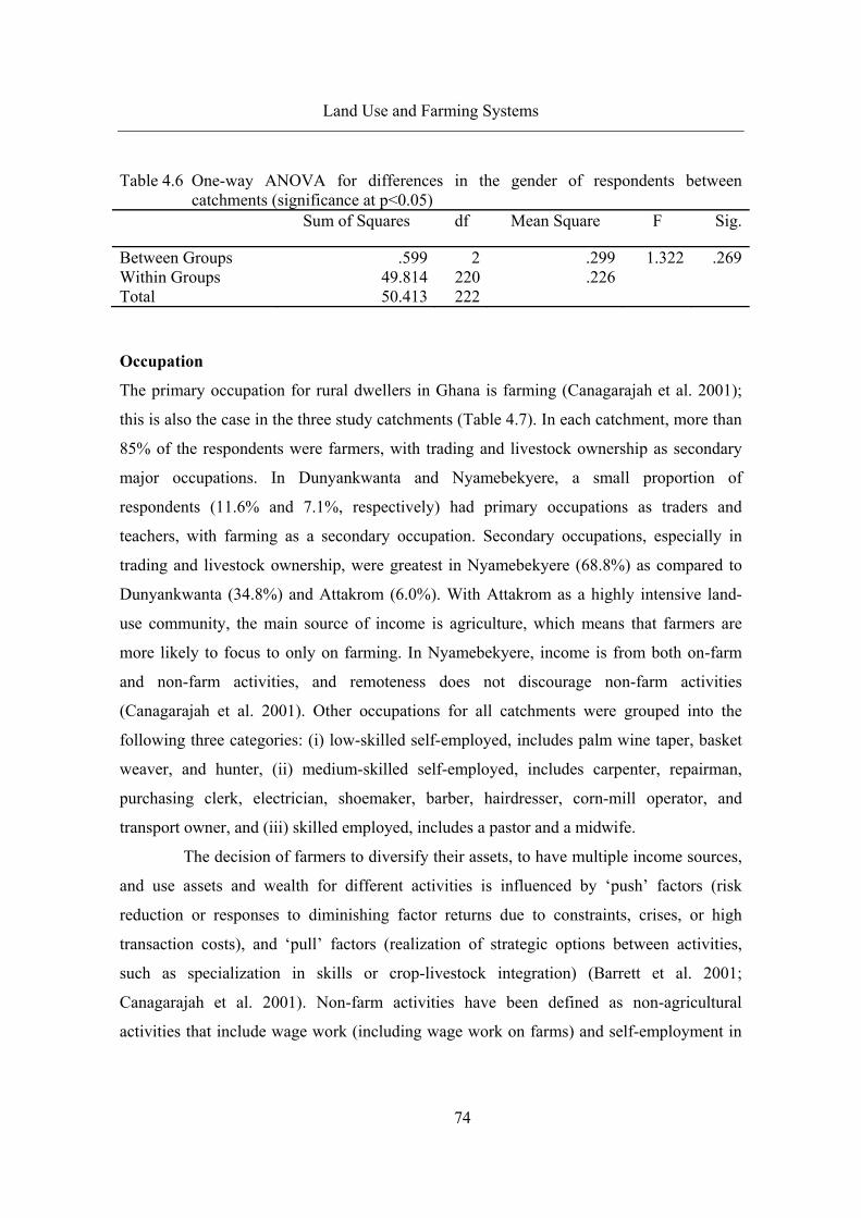
Land Use and Farming Systems

74

Table 4.6 One-way ANOVA for differences in the gender of respondents between catchments (significance at p<0.05)

Sum of Squares df Mean Square F Sig.

Between Groups .599 2 .299 1.322 .269Within Groups 49.814 220 .226 Total 50.413 222

Occupation

The primary occupation for rural dwellers in Ghana is farming (Canagarajah et al. 2001);

this is also the case in the three study catchments (Table 4.7). In each catchment, more than

85% of the respondents were farmers, with trading and livestock ownership as secondary

major occupations. In Dunyankwanta and Nyamebekyere, a small proportion of

respondents (11.6% and 7.1%, respectively) had primary occupations as traders and

teachers, with farming as a secondary occupation. Secondary occupations, especially in

trading and livestock ownership, were greatest in Nyamebekyere (68.8%) as compared to

Dunyankwanta (34.8%) and Attakrom (6.0%). With Attakrom as a highly intensive land-

use community, the main source of income is agriculture, which means that farmers are

more likely to focus to only on farming. In Nyamebekyere, income is from both on-farm

and non-farm activities, and remoteness does not discourage non-farm activities

(Canagarajah et al. 2001). Other occupations for all catchments were grouped into the

following three categories: (i) low-skilled self-employed, includes palm wine taper, basket

weaver, and hunter, (ii) medium-skilled self-employed, includes carpenter, repairman,

purchasing clerk, electrician, shoemaker, barber, hairdresser, corn-mill operator, and

transport owner, and (iii) skilled employed, includes a pastor and a midwife.

The decision of farmers to diversify their assets, to have multiple income sources,

and use assets and wealth for different activities is influenced by ‘push’ factors (risk

reduction or responses to diminishing factor returns due to constraints, crises, or high

transaction costs), and ‘pull’ factors (realization of strategic options between activities,

such as specialization in skills or crop-livestock integration) (Barrett et al. 2001;

Canagarajah et al. 2001). Non-farm activities have been defined as non-agricultural

activities that include wage work (including wage work on farms) and self-employment in

Land Use and Farming Systems

75

any non-agricultural activity, and that is significantly influenced by education, age of the

individual, location, and regional characteristics (Canagarajah et al. 2001). Observations by

Joliffe (2004) that households with higher education are more likely to work in non-farm

activities than those with lower education are also confirmed by the higher education

standards in Nyamebekyere (see next section: Education Level). Between 40% to 45% of

the average household income was achieved by non-farm activities, which is becoming an

increasingly important way out of poverty (Reardon 1997). Involvement in non-farm

activities has been associated with lower poverty, and in some situations the type of

employment is dependent on the incomes derived from agriculture (Newman and

Canagarajah 2000; Oduro and Osei-Akoto 2008). Non-farm activities in African villages

are usually first-stage activities that are a spin off from agricultural activities (FAO 1998),

although some skill-intensive activities were observed in the catchment, e.g., carpentry and

teaching.

Table 4.7 Distribution of primary and secondary occupations, and of types of secondary occupations (%)

Occupation Type Attakrom Dunyankwanta Nyamebekyere

N = 83 N = 69 N = 70Primary Farmer 96.4 87.0 92.9 Teacher 0.0 2.9 7.1 Trader 0.0 8.7 0.0 Other 3.6 1.4 0.0Secondary 6.0 34.8 68.8 Farmer 0.1 3.6 5.0 Livestock owner 0.0 1.5 14.8 Teacher 0.0 0.0 1.0 Trader 0.1 0.8 17.8 Other 0.2 2.5 8.9 None 5.6 22.7 21.5

Educational level

Literacy and the level of formal education affect the kind of information people have access

to and the range of opportunities at their disposal (UNEP 2008). Worldwide, the

educational level of a population is important in determining land-use activities, since

Land Use and Farming Systems

76

education provides more opportunities to increase income, determines the types of

livelihoods found in a community, determines the ability of an individual for skilled labor,

and also directly increases production or improves the allocation of resources to indirectly

increase production (Welsh 1970; Psacharopoulos and Patrinos 2002; Yang and An 2002).

Although studies have shown overall benefits of educating farmers, some authors have

indicated that for developing countries, these benefits are seen mostly in Asia with little or

no evidence of positive effects on productivity in Latin America and Africa (Phillips 1987;

Deininger and Olinto 2000; Jollife 2004). The influence of education is rather seen on input

use despite the market imperfections (Deininger et al. 2000), although in countries like

Ghana, the returns to education are not as significant as in other African countries such as

Uganda (Canagarajah et al. 2001). According to Jollife (2004), the fact that education

affects behavior on the farm and farm productivity has been the focus of most studies, and

non-farm benefits of education have been poorly assessed. Results from Jollife’s (2004)

study, show that in Ghana the value of education is found more in the impact on non-farm

activities, and that education increased non-farm profit far more than on-farm.

The assessment of the educational level of the respondents in the three catchments

(Table 4.8) shows a greater proportion of individuals with no or only primary education

(90.1% of respondents) in Attakrom, and a greater proportion (67.8%) with more advanced

education, i.e., from Middle School Leaver’s Certificate (MSLC) to polytechnic and

teacher training, in Nyamebekyere. This corresponds to the occupation results, where

Nyamebekyere shows a greater proportion of respondents (70%) with secondary

occupations, compared with a significantly smaller percentage (6%) in Attakrom.

Individuals who are more educated than other members in the household are less likely to

work strictly on the farm, more likely to work off the farm, and spend a larger proportion of

their working hours in non-farm activities (Jollife 2004).

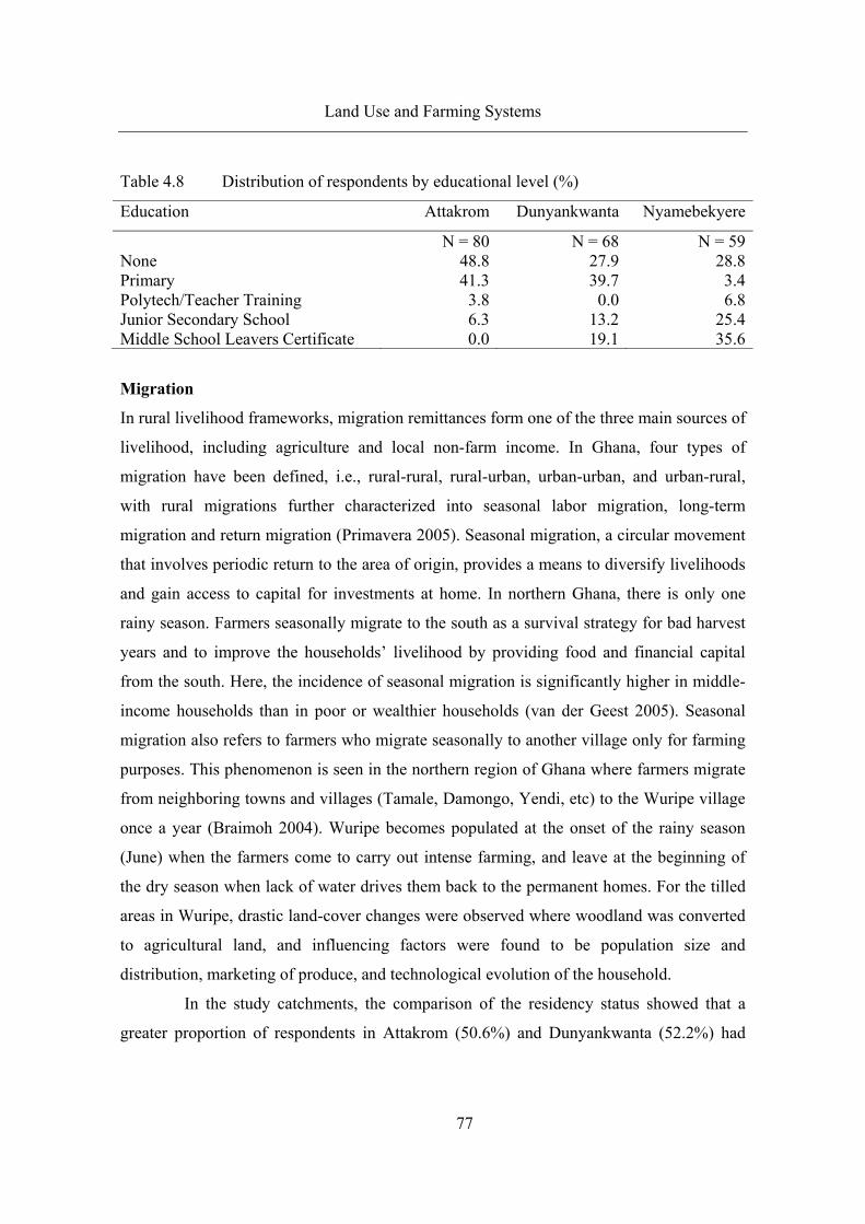
Land Use and Farming Systems

77

Table 4.8 Distribution of respondents by educational level (%)

Education Attakrom Dunyankwanta Nyamebekyere

N = 80 N = 68 N = 59None 48.8 27.9 28.8Primary 41.3 39.7 3.4Polytech/Teacher Training 3.8 0.0 6.8Junior Secondary School 6.3 13.2 25.4Middle School Leavers Certificate 0.0 19.1 35.6

Migration

In rural livelihood frameworks, migration remittances form one of the three main sources of

livelihood, including agriculture and local non-farm income. In Ghana, four types of

migration have been defined, i.e., rural-rural, rural-urban, urban-urban, and urban-rural,

with rural migrations further characterized into seasonal labor migration, long-term

migration and return migration (Primavera 2005). Seasonal migration, a circular movement

that involves periodic return to the area of origin, provides a means to diversify livelihoods

and gain access to capital for investments at home. In northern Ghana, there is only one

rainy season. Farmers seasonally migrate to the south as a survival strategy for bad harvest

years and to improve the households’ livelihood by providing food and financial capital

from the south. Here, the incidence of seasonal migration is significantly higher in middle-

income households than in poor or wealthier households (van der Geest 2005). Seasonal

migration also refers to farmers who migrate seasonally to another village only for farming

purposes. This phenomenon is seen in the northern region of Ghana where farmers migrate

from neighboring towns and villages (Tamale, Damongo, Yendi, etc) to the Wuripe village

once a year (Braimoh 2004). Wuripe becomes populated at the onset of the rainy season

(June) when the farmers come to carry out intense farming, and leave at the beginning of

the dry season when lack of water drives them back to the permanent homes. For the tilled

areas in Wuripe, drastic land-cover changes were observed where woodland was converted

to agricultural land, and influencing factors were found to be population size and

distribution, marketing of produce, and technological evolution of the household.

In the study catchments, the comparison of the residency status showed that a

greater proportion of respondents in Attakrom (50.6%) and Dunyankwanta (52.2%) had

Land Use and Farming Systems

78

migrated into the catchments, as compared to Nyamebekyere (12.9%), mainly from the

Ashanti Region (Table 4.9). Farming was the main reason given by respondents for moving

to Attakrom and Dunyankwanta, with a small percentage (<5%) indicating other reasons

such as trading, moving in with family members, and transfers (for those who were

teachers). Compared to the other catchments, a relatively larger proportion of the

respondents in Attakrom (21.7%) was non-resident, i.e., farmers who did not permanently

reside in the catchment, but owned farms and stayed for short periods (seasonal farmers).

The lower incidence of migrants to Nyamebekyere could be due to its relative isolation and

distance from major roads and markets.

Table 4.9 Respondents who are residents, have migrated, or temporarily live in catchments (%)

Residency Attakrom Dunyankwanta Nyamebekyere

N = 83 N = 69 N = 70Resident 27.8 47.8 85.7Migrated 36.1 50.7 11.4Location Neighboring town 9.5 2.8 2.5 Ashanti region 14.6 39.5 8.7 Outside region 10.3 7.1 0.0 Outside Ghana 1.7 1.4 0.0Non-resident 36.1 1.4 2.9

4.3.3 Wealth

Poverty and social inequity remain the major constraints to sustainable development in

Africa and are a major cause of environmental degradation. Poverty refers to more than the

lack of access to financial resources and material resources, and includes lack of

capabilities that allow access to income, health, education, empowerment and social

inclusion, and human rights (UNEP 2008). One common measure of poverty is wealth,

which influences a farmer’s capacity to invest in the land or financially benefit from

produce (Langyintuo and Mungoma 2006; Shilpi and Umali-Deininger 2008). Definitions

of wealth groups and indicators are often arbitrary with categories frequently based on the

researcher’s definitions. Wealth ranking methods (i.e., participatory research methods in

which community members define wealth criteria and classify themselves based on this)

Land Use and Farming Systems

79

have been recommended as being more reliable in determining wealth groups of

households (Phiri et al. 2004; Green et al. 2006).

Farm households have varying levels of different assets, each of which can

potentially contribute to the wealth status of the household. Wealth indicators, comparable

across villages, generally fall into the following categories: land distribution or land

cultivated, physical assets (such as livestock, mechanical labor, radio set, bicycle, housing

type, etc.), access to cash and credit through non-governmental organization or government

programs, income generated from livelihoods (both on- and non-farm), and expenditure

(food, farm inputs, labor, education) (Phiri et al. 2004; Green et al. 2006; Langyintuo and

Mungoma 2006). From these categories, wealth levels for this study are assessed by

internal and external income, housing status and type, livestock ownership and types of

animals, property rights and number of fields.

Income categories

The overall monthly earned income of respondents show that a greater proportion of

respondents in Nyamebekyere (65.7%) belong to the low income group (<¢400,000 or €37

per month) as compared to Dunyankwanta (56.1%) and Attakrom (48.6%) (Table 4.10). In

Attakrom, the proportion of high income (> ¢1,000,000 or €74 per month) respondents was

relatively larger than in the other two catchments. More than half of the community

(54.2%) receives frequent unearned income as compared to Dunyankwanta (22.7%) and

Nyamebekyere (15.7%), in the form of payments from family members within or outside

the community, and in a few cases, pension payments. This translates into greater financial

resources for respondents in the high land-intensity use catchment. Statistically, there was

not enough evidence to show significant differences in income levels between the

catchments at p=0.106. Differences were significant for external incomes at p<0.05%

(Table 4.11) between Attakrom and Dunyankwanta (p=0.001) and between Attakrom and

Nyamebekyere (p=0.000) (Table 4.12).

Land Use and Farming Systems

80

Table 4.10 Monthly earned income and unearned income (%) (* €1= ¢10.8)

Amount earned per month Attakrom Dunyankwanta Nyamebekyere

(¢‚000)* N = 72 N = 66 N = 70Earned Income Low <400 48.6 56.1 65.7 Medium 400 - 799 23.6 25.7 24.3 High > 800 27.8 18.2 10.0Unearned Income Yes 52.6 22.7 15.7 No 47.4 77.3 84.3 Table 4.11 One-way ANOVA for differences between catchments for earned (Ea_Income)

and unearned (UE_Income) incomes (significance at p<0.05) Sum of Squares df Mean Square F Sig.

Ea_Income Between Groups 7.887 2 3.943 2.265 .106Within Groups 356.883 205 1.741 Total 364.769 207

UE_Income Between Groups 5.643 2 2.822 14.813 .000Within Groups 39.810 209 .190 Total 45.453 211

Table 4.12 One-way ANOVA post hoc test for differences between catchments for

unearned income Dependent Variable: UE_Income

(I) Locality (J) Locality Mean Difference (I-J)

Std. Error

Sig. 95% Confidence Interval

Attakrom Dunyankwanta .29904(*) .07763 .001 .1114 .4866Nyamebekyere .36917(*) .07241 .000 .1941 .5442

Dunyankwanta Attakrom -.29904(*) .07763 .001 -.4866 -.1114 Nyamebekyere .07013 .06798 .663 -.0943 .2346Nyamebekyere Attakrom -.36917(*) .07241 .000 -.5442 -.1941 Dunyankwanta -.07013 .06798 .663 -.2346 .0943* Mean difference is significant at the 0.05 level.

Housing

Since wealthier farmers are able to own and afford better facilities, the housing status and

the quality of building material were used to assess the wealth level of the household. A

greater proportion of the respondents lived with family members in a shared home in

Attakrom (47.6%) and Nyamebekyere (44.9%). In Dunyankwanta (43.5%), the greatest

Land Use and Farming Systems

81

proportion of households owned their own homes (Table 4.13). In Nyamebekyere, there

was an average distribution between those who owned, rented or lived in family homes.

The communities were distinctly different in the quality of material used to build the

homes. In Attakrom, although mud was used by 60% of the respondents, a significant

proportion (40%) could afford more expensive materials such as brick and cement. In

contrast, only 13.4% and 11.6% in Dunyankwanta and Nyamebekyere, respectively, could

afford such materials.

Table 4.13 Housing status and type of building material for home (%) Parameter Attakrom Dunyankwanta Nyamebekyere

N = 72 N = 66 N = 70Housing status Own 35.4 43.5 27.5 Rent 17.1 17.4 27.5 Family/Shared 47.6 39.1 44.9Type of housing Mud 57.1 86.6 88.4 Brick 29.9 11.9 - Cement 10.4 1.5 11.6 Corrugated iron (Zinc) 2.6 - -

Livestock ownership

In improving livelihoods, there is an increasing complexity in the integration of crops and

livestock by smallholder farmers in response to factors such as population increase,

declining soil fertility, climate change and unpredictable weather patterns (Kruska et al.

2003; Herrero et al. 2007). Several species of livestock have different purposes, e.g., the

provision of food for the family, cash from product sales (e.g., milk, beef, and eggs), capital

assets, provision of manure, fiber for clothes, etc. In some countries, draught animals such

as oxen also contribute directly to the productivity of land (ploughing, manure) and can

increase credit access by serving as collateral (Deininger and Olinto 2000).

Nyamebekyere had the highest percentage of respondents who owned livestock

(77.1%) as compared to Attakrom (46.4%) and Dunyankwanta (37.7%) (Table 4.14), which

gave enough evidence for statistical differences between catchments at p<0.05 (Table 4.15).

Differences were significant between Attakrom and Nyamebekyere (p=0.000) and between

Land Use and Farming Systems

82

Dunyankwanta and Nyamebekyere (p=0.000) (Table 4.16). For all catchments, the order of

livestock abundance was chickens>goats>sheep. Since subsistence farming is the major

farming type in Nyamebekyere, meat supplements the protein component of diet and

livestock is considered an asset and investment for the poorer farmers in Nyamebekyere,

who belong to a relatively lower income category than those in the other two catchments.

Table 4.14 Livestock ownership and types of animals (%) (Types columns may add up to more than the total percentage, as different types of livestock are owned by individual farmers)

Types Attakrom Dunyankwanta Nyamebekyere

N = 84 N = 69 N = 70Yes 46.4 37.7 75.7 Chickens 36.9 19.3 58.6 Goats 21.4 4.4 37.1 Pigs - 1.8 1.4 Sheep 13.1 3.5 18.6 Other 7.7 - 2.9No 53.6 62.3 24.3 Table 4.15 One-way ANOVA for differences in livestock ownership between catchments

(groups) with significance at p<0.05 Sum of

Squares df Mean Square F Sig.

Between Groups 6.059 2 3.030 13.481 .000Within Groups 49.439 220 .225 Total 55.498 222 Table 4.16 One-way ANOVA post hoc test for differences between catchments for

livestock ownership (Dependent Variable: Livest_own ) (I) Locality (J) Locality Mean Difference (I-J) Std. Error Sig.

Attakrom Dunyankwanta -.08747 .08031 .623 Nyamebekyere .30714(*) .07451 .000Dunyankwanta Attakrom .08747 .08031 .623 Nyamebekyere .39462(*) .07752 .000Nyamebekyere Attakrom -.30714(*) .07451 .000 Dunyankwanta -.39462(*) .07752 .000* Mean difference is significant at the 0.05 level.

Land Use and Farming Systems

83

Property rights

Property rights to resources such as land, water, and trees are important factors in the role

of poverty reduction, resource management and environmental management linkages. They

may constrain or facilitate sustainable use, protection or resource improving investments, as

well as determine welfare of the households who depend on these resources (World Bank

2006). In the Ashanti Region, property rights are communal with land ownership by the

‘Amakomhene’ (chief) and administration by the village head or the ‘Odikro’. The

sharecropping system (produce is shared between the sharecropper and landowner at a ratio

of 2:1) is more important to the farmers, although other types of land-tenure systems are

available (Meijerink et al. 2003). The family land inheritance is free to use as desired

except when leased, and in this case the chief has to be part of the agreement. In share

tenancy, food crops are for the farmer and tree crops for the land owner; in rentals, the

farmer compensates the land owner by an agreed measure. Food crops on stool lands are

solely for the benefit of the farmer, but this is not as common due to unavailability of land.

Renting of land is also available but there is no standard rent and costs range depending on

the size of the field, the fields are to be used only for food crops.

According to the VINVAL study, more than 50% of the Attakrom community

practices sharecropping, normally applicable to non-permanent crops. Currently, with the

commercialization of food crops, cash payments are being demanded by landowners and

have caused the intensification of agricultural activities by the sharecroppers to maximize

benefits. Landowners also try to maximize benefits from the land and give out the land

irrespective of its cropping history. In Dunyankwanta, 90% of the community own land

through family inheritance, with 50-60% involved in land tenancy where farmers cultivate

cocoa for the land owner and food crops for themselves. In Nyamebekyere, the ‘taungya’

system allows farmers to cultivate any area they wish as long as they replant young forest

tree saplings in assigned areas within the catchment. The saplings are provided by the

Forestry Department.

Land Use and Farming Systems

84

Number of fields per household

In Attakrom, a greater proportion of the population farmed on only one field (Table 4.17).

In Dunyankwanta, there was an almost even spread of respondents who farmed between 1

and 3 fields, and in Nyamebekyere, a larger percentage of the households farmed on 2

fields. Fields in Attakrom were generally rented, in Dunyankwanta they were family lands,

and in Nyamebekyere, there was an even distribution between family land, rentals and

government-provided land.

In Nyamebekyere, the land is within the forest reserves, although the local farmers

have been allowed to pursue subsistence farming by the government, and pay for this by

planting secondary trees. The ‘other’ status refers to the situation where a farmer owns

some of the land and rents it or is a laborer in another, a situation which is more common in

Dunyankwanta and Nyamebekeyere. In all the catchments, field sizes were on average

between 1-5 acres (0.405-2.023 hectares).

Table 4.17 Property rights, number of fields and size of fields (%) Parameter Attakrom Dunyankwanta Nyamebekyere

N = 83 N = 62 N = 67Land ownership Family land 28.0 58.1 32.8 Government 3.7 - 22.4 Laborer 19.5 8.1 3.0 Rent 42.7 8.1 34.3 Other 6.1 25.8 25.8Number of fields 1 52.4 28.4 24.3 2 27.4 31.3 41.4 3 15.5 29.9 25.7 4 3.6 7.5 8.6 >5 1.2 3.0 -Size of fields (acres)* 1-5 62.9 71.6 59.9 6-10 26.5 17.6 25.2 11-15 5.3 4.7 6.8 16-20 4.0 0.7 4.8 21-25 0.7 5.4 1.4 >25 0.7 - 2.0* 1 acre = 0.405 hectares (or 0.004 km2)

Land Use and Farming Systems

85

4.3.4 Farming and cropping system

This section summarizes the responses of the interviewed farmers about factors that

influence soil properties and may affect nutrient export from soils into the aquatic system,

i.e., types of crops and fallow periods, fertilizer and pesticide use, and livestock ownership.

For precise information on the actual differences in nutrient contents of the soil in the three

catchments, detailed research would be required to analyze individual farmland soil

properties and soil nutrient content. However, as the purpose of the research was to

compare the differences in socio-economic characteristics and behavior of farmers that

would contribute to overall nutrient input within each catchment, it is assumed that the

differences in these activities would be reflected in different levels of Impact (measured as

total nutrient loading in the streams), without the need to analyze farmland soils for definite

quantities in nutrient levels.

Fallow and land preparation

Traditionally, long fallow periods were used to restore soil quality and yield levels, but with

demographic pressure, the number of fallow years has been shortened such that fallowing

alone is not sufficient to maintain soil fertility (Nubukpo and Galiba 1999). With the

decreasing land availability and option for long fallow, Drechsel et al. (2005) presumed that

soil management practices (e.g., fertilizer input) would intensify, since most farmers (80%)

were aware of declining yields due to decreasing fallow periods. The authors, however,

found no significant relationship between the length of fallow periods and farmers’ soil

fertility management practices, although there were a few incidences of fertilizer

application, explained as either compensation for shortened fallow periods or more

fertilizer accessibility in areas where fallow periods were shorter (close to the urban areas,

e.g., the city of Kumasi).

From the interviews, post-harvest activities in the catchments were classified into

one of four categories: (i) immediate replanting after harvesting mature crops on

intercropped fields, (ii) replanting of crops, done at the same time of the year and mostly on

intercropped fields, (iii) retaining only tree crops on fields after food crops were harvested,

since trees had relatively longer life spans, and (iv) fallowing, where the entire field is left

Land Use and Farming Systems

86

for a period depending on the history of its use. Only two farmers out of all respondents

interviewed indicated that the land was returned to the owner after harvest. On fields that

had only one crop, fallow periods ranged between 3 months to 3 years depending on the

crop in Attakrom (27.6%) and in Dunyankwanta (9.0%) (Table 4.18). In Nyamebekyere,

most respondents indicated that replanting was immediately after harvest, with no fallow

periods. Most of the farmers in all the catchments practiced intercropping, which means

that harvesting periods varies for different crops, and fallowing cannot be carried out on

these fields. In addition to restoring soil fertility, re-growth of natural vegetation during

fallow periods helps in the control of weeds (Styger and Fernandes 2006). Studies have

shown that fallow periods of >3 years are more effective at weed control than periods of ≤3

years (Awanyo 2008). This is because the larger pool of tree seeds in soils leads to a greater

recruitment of trees in the longer fallow periods, which shade out weeds and reduce weed

seed production. As weed infestations increase with reduced fallow periods, many farmers

use fire during land preparation to control weed growth. The slash-and-burn technique also

provides nutrient-rich ashes, which are used on crops in the fields, and in some areas only

on higher value crops in multiple-cropping fields (Drechsel and Zimmerman 2005).

Mulching (keeping weed and crop residues on the field) is being promoted as an alternative

method being more effective in controlling weeds, maintaining soil fertility and saving

labor costs (Ekboir et al. 2002), but it is still not widespread in Ghana. Burning leaves the

soil bare and recruitment of weed seeds is high, whereas with mulching, germination is

suppressed.

In this study, land preparation was mainly by slash and burn, with planting carried

out immediately after. In Attakrom, preparation included the felling of trees (3%), and the

application of herbicides within approximately two weeks after burning. For fields that had

multiple crops, weeding was continuously carried out under young plants or tree crops that

remained on the land after harvest. For some of the tree crops (cocoa and orange),

herbicides were applied once a year to control weeds. According to Awanyo (2008),

although frequent weeding was effective in suppressing weeds, it was rather how careful

the weeding was done that was more important. Due to the labor-intensive process of land

preparation, i.e., clearing of vegetation and burning, some farmers mentioned that laborers

Land Use and Farming Systems

87

were hired to clear the fields. Labor, one investment in the intensification of cultivation (the

other being the application of nutrients), is related mainly to land clearing and weeding but

not to any other farming input tasks (Drechsel and Zimmerman 2005), and requirements

depend on the kind of vegetation that needs to be cleared (i.e., trees or grasses and

broadleaf weeds).

Table 4.18 Post harvest and fallow (%) Activity Attakrom Dunyankwanta Nyamebekyere

N = 76 N = 67 N = 62Immediate replanting 61.8 19.4 98.6Planting same time each year 7.9 37.3 0.0Tree crops left on land 2.6 34.3 0.0Fallow 27.6 9.0 1.4

Major crop types

In general, farmers growing commercial crops are more likely to invest in soil fertility

improvement (e.g., fertilizers) as a means to improve returns from the harvest (Kelly 2006).

In Ghana, agricultural production is typically of traditional export crops (cocoa and oil

palm), traditional non-export subsistence crops (yam, plantain), and non-traditional export

crops (fruits, vegetables and root crops). In most villages in Ghana, farmers do not

specialize in specific crop types but rather produce a wide range of crops (Oduro and Osei-

Akoto 2008). Compared to the past, declining trends have been observed in cocoa

production with increased growth in oil palm (as an export crop) and more nutrient- and

moisture-efficient crops (e.g., cassava) as subsistence and cash crops. The decline of cocoa

productivity, due to the fact that landowners have no resources for replanting dying trees,

has led to more interest in traditional crops that can be used as cash crops. These include

tree crops such as citrus and oil palm, and recently rice crops (Meijerink et al. 2003). The

general increase in sharecropping is also a response to the decline of cocoa productivity, as

tenants provide extra labor and invest resources into the land.

For each catchment, the ranking of importance of different crops by the VINVAL

project and the results of this research for the top ten crops (total percentage of farmlands

on which the crops were grown) were compared (Table 4.19). Major cropping systems

Land Use and Farming Systems

88

include (i) traditional food crops maize, cassava, plantain and cocoyam, (ii) newly

emerging cash crops such as rice and vegetables (okra, pepper), and (iii) the tree crops

cocoa, citrus and oil palm (Meijerink et al. 2003). The principal crops grown by the

interviewed farmers (cultivated on 30-45% of the farms) were cassava, cocoa, and plantain.

An additional crop was maize in Attakrom and Nyamebekyere, and cocoyam in

Dunyankwanta. Although these were the most common crops, ranking in the VINVAL

project showed different farmer preferences. For example, cocoa and maize were ranked as

the most preferred crops in both Attakrom and Dunyankwanta due to its higher commercial

value; however, cassava and plantain were the most grown crops (ranked 4th and 5th by the

farmers). These crops serve beyond household subsistence requirements as cash crops and

can be regularly harvested, in comparison to the seasonal cocoa. Cocoyam is a high cash

earner in the lean seasons (Meijerink et al. 2003). On the other hand, in Nyamebekyere,

preferences and common crops grown corresponded; plantain (84.4%) and cocoyam

(76.2%) were the most dominant food crops, and ranked as the 1st and 2nd preferred crop,

respectively, by the VINVAL project.

In most cases, mixed tree cropping was practiced, i.e., tree crops were grown

together with a minimum of two or three food crops on the same field. The types of crops

grown were similar within the three catchments, with the exception of pineapple, which

was not found at any of the farms in Attakrom, and rice in Nyamebekyere.

In Ghana, there has been a rapid increase in pineapple production due to incentives such as

the exemption from non-traditional crop export duty, a growing domestic market for

pineapple juice processing companies, and it not being as labor intensive as other non-

traditional crops (Takane 2004). Rice, a relatively new cash crop, requires a considerable

investment in herbicides and labor, and was found on fewer farms in Attakrom (6.6%) and

in Dunyankwanta (2.0%), with none observed in Nyamebekyere. On one rice field in

Attakrom, for example, the farmer spent her entire day shooting birds with a hand-made

sling, as other methods such as scarecrows (rags or clothes on sticks) did not work.

Land Use and Farming Systems

89

Table 4.19 Comparison of the importance of different crops for farmers between the VINVAL project (ranking; 1 highest, 6 lowest) (Meijerink et al. 2003) and research results (% total number of respondents that cultivate the crop).

Crop type Attakrom Dunyankwanta Nyamebekyere Study (%) VINVAL Study (%) VINVAL Study (%) VINVAL Cassava 42.4 4 47.3 3 40.8 3 Cocoa 35.8 1 43.9 1 38.8 6 Cocoyam 31.1 6 31.1 5 76.2 2 Maize 36.4 2 27.0 2 10.2 4 Oil palm 19.2 -- 6.8 -- 15.1 -- Okra 3.3 -- - -- - -- Orange 8.0 -- 6.1 -- 6.1 5 Pepper 2.7 -- 9.5 -- 28.6 -- Pineapple - -- 4.7 -- 13.6 -- Plantain 43.1 5 33.8 4 84.4 1 Rice 6.6 3 - 6 - - Yam - -- 13.5 -- 17.0 -- - food crop not mentioned by respondents -- food crop grown but of lower ranking/percentage than 6

Manure use

Intensity of livestock rearing within a catchment can be an important contribution to soil

nutrients depending on the amount of manure generated. Manure is an important source of

nutrients, as it maintains and replenishes soil fertility for crop production, and has been an

old technology in parts of Africa, where farmers practice mixed livestock and crop farming

(Brouwer and Powell 1998; Lupwayi et al. 2000; Mando et al. 2005; Mkhabela 2006;

Rufino et al. 2006). In Ghana, manure use is more common in the northern region, although

its use is found in parts of the south-western region where commercial poultry farming is

predominant (FAO 2005). It has shown success when applied to crops such as cowpea, and

may be an important source of fertilizer throughout Ghana in the near future.

In the three study catchments, however, manure (poultry, sheep and goat manure)

was not considered a useful resource by most of the communities and was rather discarded,

except by a few farmers (<2% of all respondents). Manure collected from pens was usually

dumped at a general dump site away from the community within the catchment (although

not near the streams). Discussions with farmers indicated that agricultural extension

officers had tried to educate them on the use of manure, but this had not been accepted by

the farmers, although the reason why was unclear. The trend of low manure use

Land Use and Farming Systems

90

corresponds with results for areas located near the study sites, where less than 5% of the

farmers applied manure to fields (Drechsel and Zimmerman 2005). According to that study,

the labor- and time-consuming collection and transport was not considered worthwhile by a

majority of the farmers, as quantities were generally small and fields were far away from

the compounds. Factors that negatively affect the farmers’ decision to use manure include

farm size, distance of fields to the homestead, proportion of cultivated land recently under

fallow, labor and transport requirements for handing manure, lack of technical information

on fertilizer value and management of manure, increased growth of weeds, and bad smell

(Williams 1999; Mkhabela and Matereschera 2003; Abdoulaye and Sanders 2005). The

collection of the manure and transport to the farm sites is considered a tedious process

requiring the use of extra labor, with the perception of the returns not immediately apparent

to the farmers (Abdoulaye and Sanders 2005; FAO 2005).

Pesticide use

Weeds compete with the crops for soil nutrients, and increased weed growth promotes

diseases (insect attacks) and high humidity which, in Ghana, encourages the ‘black pod’

disease (Fosu et al. 2007). Although the assessment of toxic chemicals in streams was not

part of this research, farmers’ responses about pesticide use contributes to the

understanding of the priorities of farmers in relation to investments in crops and land-use

intensity. Attakrom had the highest use in pesticides (68.8%) followed by Dunyankwanta

(43.5%), with minimal use in Nyamebekyere (2.9%) (Table 4.20). The most common

reason for no use was that the farmer could not afford pesticides, although most farmers are

aware of their benefits. Statistically, there were significant differences in pesticide use

between the three catchments at p<0.05 (Table 4.21; Table 4.22).

Land Use and Farming Systems

91

Types of pesticides used in the catchments include the following;

(i) Herbicide – Condemn, Power, and Roundup (active ingredient glyphosate) belong to a

group of broad spectrum herbicides usually used before planting, as part of the land

preparation process. Atrazine is a selective herbicide, with active ingredient atrazine,

used after planting to control broad leaf plants and grass.

(ii) Fungicide – Champion, Fungrian, Foko, and Kocide prevents fungal growth on crops.

Champion and Kocide have the copper based active ingredients (copper hydroxide), and

Foko and Fungrian are manganese-based.

(iii) Insecticide – Thionex for general control and Dursban (Chloropyrifos) usually for the

prevention of termite infestation. Active ingredients include endosulfan. Although DDT

has been banned, 3 of the farmers apparently still had access to it (or probably used

DDT as a generic name for pesticides). In the national annual monitoring and

assessment program for 2005, high values of DDT (0.4 mg L-1) were, in a few cases,

recorded in parts of the south-western basin systems, which is above the WHO

guideline value of 0.001 mg L-1 (Ansa-Asare and Darko 2006). According to the report,

these high values need to be assessed.

The most popular pesticides applied in the catchments were Atrazine, Kocide,

and Roundup. Land preparation generally is done by manual weeding using cutlasses, and

those who can afford it use Roundup approximately 3 weeks after weeding, before the

planting season begins. Roundup is also used to clear the weeds under the tree crops, i.e.,

cocoa, orange and oil palm. Atrazine is applied on an average of 8 weeks after planting, and

mainly to crops such as maize, cassava, plantain, cocoyam and rice. Kocide is usually

applied on the tree crops cocoa and orange once a year, although some farmers applied it

frequently to vegetables. One source of worry for cocoa farmers is the fungus Phytophthora

which causes canker of the stem and in mummified dry pods, husks and roots (Fosu et al.

2007). Two types are found in Ghana – P. palmivora which is less destructive and lives in

the flower cushions and P. megakarya which is more destructive and survives in the soil.

Kocide is typically applied in May when the fungus appears.

Land Use and Farming Systems

92

Table 4.20 Pesticide use in the last 2 years (2004-2006), types used, and the reasons given by respondents who answered ‘No’ (%). (Types columns may add up to more than the total percentage as multiple types of pesticides was used by individual farmers)

Pesticide Use Attakrom Dunyankwanta Nyamebekyere

N = 79 N = 63 N = 69Yes 70.9 44.4 2.9 Types Atrazine 31.6 23.8 - Champion 2.6 6.3 - Condemn 5.0 7.9 1.5 DDT 2.6 - 1.5 Dursban 2.6 - - Foko 3.8 - - Fungrian 7.6 - - Insecticide 2.6 - - Kocide 21.6 4.8 1.5 Power 5.0 - - Roundup 34.2 7.9 - Thionex 1.3 6.3 -No 29.1 55.6 97.1 Reasons Cannot afford 27.6 48.9 95.6 No need 1.5 6.7 1.5 Table 4.21 One-way ANOVA for differences in pesticide use between catchments (groups)

(significance at p<0.05) Sum of

Squares df Mean Square F Sig.

Between Groups 17.146 2 8.573 52.756 .000Within Groups 33.801 208 .163 Total 50.948 210

Land Use and Farming Systems

93

Table 4.22 One-way ANOVA post hoc test for differences between catchments for pesticide use

Dependent Variable: Pesticide (I) Locality (J) Locality Mean

Difference (I-J)Std. Error Sig.

Attakrom Dunyankwanta -.26442(*) .08141 .004 Nyamebekyere -.67988(*) .05532 .000Dunyankwanta Attakrom .26442(*) .08141 .004 Nyamebekyere -.41546(*) .06631 .000Nyamebekyere Attakrom .67988(*) .05532 .000 Dunyankwanta .41546(*) .06631 .000* Mean difference is significant at the 0.05 level.

In Ghana, an estimated 87% of farmers use a wide range of chemicals as

herbicides, fungicides and/or insecticides (Dinham 2003). As also observed in this study

(Table 4.23), herbicides are the predominant pesticide type in Ghana. Herbicides are

perceived to perform longer, be more effective over a wider area than manual weeding, and

result in reduced time, cost and labor (Ntow et al. 2006). Pesticides are available in

agricultural retail stores, and a few pesticide sellers measure out smaller quantities for sale

to those who cannot afford the entire container. Information about pesticide application

comes from pesticide sellers, agricultural extension officers, pesticide labels and other

farmers. The amounts applied vary depending on the farmer, crop and application time,

with applications either by knapsack (for those who can afford it) or spraying bottles. Some

farmers randomly mixed the pesticides, with the understanding that this makes them more

effective, especially when cheaper brands and smaller quantities are all that can be

afforded. Although many farmers use chemical pesticides in Ghana, it is not used correctly

since most have received no training in use and application, which affects making proper

decisions on pesticide selection and leads to poor application and timing rates, and health

risks (Ntow et al. 2006).

Land Use and Farming Systems

94

Table 4.23 Pesticide types used (%). Columns add up to more than total percentage since each respondent used more than one type of pesticide.

Pesticide Name Attakrom Dunyankwanta Nyamebekyere

Herbicide Atrazine Condemn

Power 75.8 15.9 1. 5

Roundup Fungicide Champion

Foko Fungrian Kocide

35.6 11.1 1.5

Insecticide Dursban Thionex 3.9 6.3 0.0

Fertilizer use

In Ghana, fertilizer use has fluctuated over the past few decades. Under the agricultural

policies of the 1970’s and 1980’s, major production incentives for increased input use

existed for farmers and included fertilizers, improved seeds, and bank loans administered

by public agencies. In the early 1980’s, fertilizers was sold to farmers at about half the price

agencies had to pay. From 1987 onwards, subsidies were gradually removed, ending

completely in 1989. By 1999, there was a reduction of 48% of total fertilizer use. In 2008,

the government re-introduced fertilizer subsidies of 40-50% for poor smallholder farmers.

Although subsidized, incentives for purchasing and applying fertilizers are fundamentally

the fertilizer yield response and input and output prices (Kelly 2006). Farmer knowledge

and experience with fertilizers will affect the perception of the yield response and

profitability, which is generally lower than that perceived by researchers and extension

personnel. The incentives are also shaped by relative returns, such as profitability, as

compared to other non-farm or health-related opportunities. These returns are influenced by

different management practices by different farmers, changes in climate and soil quality,

output prices that are usually volatile and can fluctuate from season to season, and even the

variability in the prices of fertilizers in space and time. The use of fertilizers in Ghana

varies according to the region, with the Upper regions being the largest consumer, due to

the production of vegetables under irrigation during the dry season in the Upper East (FAO

2005). Maize accounts for 40% of fertilizer use on food crops.

Land Use and Farming Systems

95

For the study catchments, fertilizer use in 2004-2006 was higher in Attakrom (20.5% of

respondents) than in Dunyankwanta (12.3%) and Nyamebekyere (0%) (Table 4.24), a

phenomenon also observed by the VINVAL project (Meijerink et al. 2003). There is

enough evidence to show significant differences in fertilizer use between catchments

(p<0.05) (Table 4.25), which forms the basis for this study’s hypothesis that nutrient levels,

physico-chemistry and macroinvertebrate community dynamics varies significantly.

Differences are significant between Attakrom and Nyamebekyere (p=0.000) and between

Dunyankwanta and Nyamebekyere (p=0.012) (Table 4.26).

When asked about the reasons for their lack of fertilizer use, a greater proportion

of farmers indicated that they could not afford fertilizers. However, financial capital is not

the only reason that farmers do not purchase fertilizers. There are also no incentives for the

farmers to risk investment in production, as fertilizer prices are unstable, market prices

fluctuate and there may be other priorities such as health and children’s education (Kelly

2006). Another main reason, which is supported by Drechsel and Zimmerman (2005), is the

perception of farmers that there is no need for fertilizers, since they are used only for a

short time in the shifting cultivation cycle. In the above study, a smaller percentage of

farmers (18%) also indicated reduced food quality (e.g. of cassava), lack of information

about fertilizer use (10%), increased weed growth (5%), and degradation of soil quality

(2%). In Attakrom and Duyankwanta, NPK/15-15-15 was the most common fertilizer,

followed by ‘asasewura’ (a premixed cocoa fertilizer), and ammonium sulphate. The

formulation of Asasewura is 0-18-22 plus calcium, sulphur and magnesium, and has been

significant in increasing cocoa yields (FAO 2005). All fertilizers used in Ghana are

imported, with the most important group being the NPK compound fertilizers, followed by

ammonium sulphate and muriate of potash (FAO 2005). Major importers of fertilizers are

private companies (80%), some commercial farms, and the Agricultural Development Bank

(ADB) that imports either for their clients or for their own use.

In the catchments, fertilizers were applied mostly to cocoa and maize, with a few

applications (approximately 6%) to rice, orange, pepper and oil palm. Since cocoa and

maize are cash crops, investment in fertilizers provides greater returns than for subsistence

crops. One farmer, however, used fertilizer on all his crops, which included cassava, oil

Land Use and Farming Systems

96

palm, cassava, pineapple, plantain, yam and cocoyam. Fertilizer application for cocoa is by

broadcasting, i.e., granules are spread around in the beds of large plants. Fertilizers used on

cocoa were Asasewura and NPK/15-15-15 that were applied to the plants once a year,

usually at the onset of the rainy season in June. The fertilizer amounts applied varied per

farmer, and responses ranged from 1 bag (50 kg) per 4 acres (1.6 hectares) to 2 bags per

acre (0.4 hectares). Fertilizer application for maize is by spot/ring application, where

granules are placed 5-30 cm away from the base or in a ring around the plant. Maize is

usually planted between April and June, before or after the rains start, with harvesting 4-5

months later. NPK 15-15-15 is usually applied to maize 2 weeks after planting; ammonium

sulphate was applied 6-8 weeks after planting. For other crops, applications for the tree

crops oil palm and oranges, and for pepper and rice are once a year at the start of the rainy

season.

The logistical regression analysis was applied to explain the use of fertilizer in the

catchments. In addition to high correlation with pesticide use, other important variables are

farm loans, access to agricultural extension officers, land status and residency, in order of

decreasing significance (Table 4.27). The model explained 94.1% of the variability at

p<0.05.

Table 4.24 Fertilizer use in the last 2 years (2004-2006), types used, and the reasons given by respondents who answered ‘No’ (%)

Fertilizer Use Attakrom Dunyankwanta Nyamebekyere

N = 83 N= 65 N = 70Yes 20.5 12.3 0.0Types Asasewura 4.8 1.5 - 7-7-7 1.2 - - NPK/15-15-15 13.3 10.8 - NH42SO4 4.8 1.5 - NPK + Foliar 1.2 - -No 79.5 87.7 100.0Reasons Cannot afford 54.7 87.0 88.2 Land fertile 43.8 13.0 11.8

Land Use and Farming Systems

97

Table 4.25 One-way ANOVA for differences in fertilizer use between catchments (significance at p<0.05)

Sum of Squares df Mean Square F Sig.

Between Groups 1.600 2 .800 8.374 .000Within Groups 20.533 215 .096 Total 22.133 217

Table 4.26 One-way ANOVA post hoc test for differences between catchments for fertilizer use

Dependent Variable: Fertilizer (I) Locality (J) Locality Mean Difference (I-J) Std. Error Sig.

Attakrom Dunyankwanta -.08174 .06060 .448 Nyamebekyere -.20482(*) .04457 .000Dunyankwanta Attakrom .08174 .06060 .448 Nyamebekyere -.12308(*) .04107 .012Nyamebekyere Attakrom .20482(*) .04457 .000 Dunyankwanta .12308(*) .04107 .012* Mean difference is significant at the 0.05 level. Table 4.27 Logistic regression of association between fertilizer use and various parameters

(Ea_Income = earned income, UE_Income = unearned income, Land_own = land ownership, Agric_Ext = agricultural extension officers, Farm_loan = access to farm loan, Livest_own = livestock ownership). df = degree of freedom; Sig = significance, at p<0.05.

B S.E. Wald df Sig. Exp(B)

Step 1(a)

Gender .824 1.133 .529 1 .467 2.280Age -.775 .418 3.442 1 .064 .461Education -.435 .283 2.358 1 .125 .647Ea_Income .363 .322 1.275 1 .259 1.438UE_Income .576 .873 .435 1 .510 1.778Migration -1.630 .752 4.704 1 .030 .196Land_own 1.227 .554 4.897 1 .027 3.410Pesticide 3.252 1.173 7.691 1 .006 25.842Agric_Ext 2.696 1.081 6.218 1 .013 14.823Farm_loan 5.065 1.648 9.445 1 .002 158.407Livest_own -1.108 .956 1.345 1 .246 .330Constant -11.767 4.713 6.235 1 .013 .000

Land Use and Farming Systems

98

4.3.5 Water resources and sanitation

Water is an important environmental resource for development, linked to poverty, human

welfare and health, and impacts household labor due to the efforts to obtain it (Madulu

2003). Potable water for all three catchments is obtained from boreholes, which have

mechanized pumps provided by the government, with a few farmers depending on hand-

drawn wells dug in the fields. Stream flow is seasonal in the catchments, and the

availability of a reliable source of potable water in the village provides a measure of

security and increased standard of living for the residents. The labor costs required for

obtaining and transporting water is reduced, and the relative quality of groundwater

compared to stream water ensures a healthier community. Overall, respondents were

satisfied with the quality of water, which in their perception ranged from good to excellent.

To maintain the running costs of the boreholes and repairs when there is a problem,

communities in Attakrom and Nyamebekyere are charged a minimal fee for the use of the

boreholes. These fees range from >¢1000 (€0.10) per year in Nyamebekyere to ¢100-¢500

(€0.01-€0.05) per use in Attakrom. In Dunyankwanta, there is no payment for water. Water

is stored by households in containers or tanks and does not require any form of

pretreatment before or during use. In circumstances when there is a temporary breakdown

of the borehole pump, residents of the communities obtain water from other parts of the

village, or nearby villages within the vicinity.

With regard to sanitation, refuse dumping and sewage were compared for each of

the catchments. Refuse is usually dumped away from the living areas of the communities at

a specified dump site, which is not located near any of the streams in both Attakrom and

Nyamebekyere. In Dunyankwanta, farmers were aware of and complained of refuse being

dumped near streams, which in their estimation leads to diseases and poor water quality;

and that there was the need for stricter rules by the District Assembly to prevent this. All

the communities have an established place of convenience – the pit latrine in

Nyamebekyere, the KVIP in Dunyankwanta, and a range of facilities at Attakrom (KVIP,

pit latrine, water closet). In Nyamebekyere and Dunyankwanta, all the facilities are public

and use is free of charge. In Attakrom, there are a few private owned water closets and,

Land Use and Farming Systems

99

although some of the public facilities are free, others charge a fee ranging between ¢100

and ¢500 per use, whilst others go to the bush as an alternative place of convenience.

With the exception of Nyamebekyere, due to the inconsistency of stream flows,

most farmers in Attakrom and Dunyankwanta use the streams during the rainy season for a

variety of purposes (Table 4.28), such as mixing the herbicides for spraying, washing,

bathing, cooking, and drinking when on the fields. From discussions, approximately 20% of

the respondents from Attakrom and Dunyankwanta, but none of the respondents from

Nyamebekyere, were aware that activities of their communities could affect the quality of

the streams and downstream communities. These farmers were aware that the applied

chemicals could be washed into the streams, and a few farmers complained that at times

fishing was done illegally with the use of chemicals (chemicals poured in the stream kill

fish, which float up for easier retrieval). Most of the farmers were also aware of the

implications of farming too close to the streams, since flooding periodically destroys the

crops. Downstream sites , with intermittent stream flow, had boreholes constructed within

the past few years by the government, but communities along sites on the Ofin River with

perennial flow, depend mostly on the river for all domestic use. In most of the downstream

sites, villagers complain of skin diseases and bloody urine, especially among the children

who swim in the river.

In the three catchments, traditional regulatory measures still function as a method

of controlling communities and their interaction with the environment, even though there is

the general impression that traditional laws are slowly losing authority. Every week, one

day is assigned a ‘no farming day’, dedicated to the earth gods - Tuesdays in Attakrom and

Dunyankwanta, and Fridays in Nyamebekyere. No one is allowed to work on the farm (i.e.,

weeding or clearing) although some allowance is given for minimal harvesting. Menstrual

women are forbidden to go near the streams until the end of their cycle, and on Tuesdays,

women cannot cross any of the streams nor can any person collect water from the stream.

Animals are not allowed near the streams, and fines are imposed on the owners of animals

that are found free range during prohibited hours, i.e., between 6 a.m. and 3 p.m. daily. To

protect the forests, most of the community members are forbidden to enter, with the

Land Use and Farming Systems

100

exception of ‘authorized persons’. Offenders are sanctioned and have to pay a fine of

usually rum and other drinks in addition to a ‘cleansing’ by the slaughter of animals.

Table 4.28 Stream use in the catchments (%) Stream Use Attakrom Dunyankwanta Nyamebekyere

N = 79 N = 69 N = 67Yes 75.9 60.9 3.0No 24.1 39.1 97.0

4.4 Summary

The farming/cropping systems were evaluated for each catchment as a function of land-use

intensification. Land preparation, as in most parts of sub-Saharan Africa, is by weeding,

burning, and clearing. The crops types are comparable across catchments, with cassava,

cocoa, plantain and maize being the major crops on 30-45% of the fields. Intercropping is

common, either with other vegetable crops or tree crops such as cocoa, oil palm, and

orange. The catchments are located within the same administrative district (Ahafo-Ano

South District) and share similar cultural and institutional setups. However, a large

proportion of the farmers in Attakrom benefited more from institutional facilities, i.e.,

access to agricultural extension officers and bank loans, than Dunyankwanta or

Nyamebekyere, where none of the respondents benefited from these services. Market

access and proximity were better for Attakrom and Dunyankwanta and limited for

Nyamebekyere.

In Attakrom, a greater proportion of the respondents (28.6%) were between 50

and 59 years old, were exclusively farmers (96.4%) who on average had basic education

(90.1%), and had an even distribution of earned and unearned income (from family

members or pension schemes). Sharecropping (produce shared between the sharecropper

and landowner at a ratio of 2:1) was the most common form of land arrangement in

Attakrom, and the proportion of respondents who use pesticides (70.9%) and fertilizers

(20.5%) were highest.

In Dunyankwanta, respondents were mostly 40-49 years old, were predominantly farmers

(87%) although 34.8% had secondary occupations. Education was mainly basic (67.6%).

Land Use and Farming Systems

101

Compared to the other catchments, a larger percentage of the respondents (50.7%) had

migrated into the catchment mostly for farming purposes. More than half the respondents

were in the low earned income category (56.1%), and 22.7% with unearned income.

Livestock ownership was the lowest compared to the other catchments (37.7%), and land

arrangement was mainly by share tenancy, where farmers grow vegetables among tree

crops that belong to the land owner. The proportion of respondents who use pesticides

(44.4%) and fertilizers (12.3%) were comparatively lower than Attakrom.

In Nyamebekyere, the majority of respondents were 40-49 years old (27.1%). Of

the three catchments, a greater proportion had secondary occupations (68.8%) in addition to

farming (92.9%). Education was the highest of all catchments, with a larger proportion of

the respondents having secondary level education (61.0%). Migration was the lowest

(11.4%), and mainly due to teacher transfers. The number of respondents in the low earned

income category was the highest (65.7%), and only 15% reported receiving any form of

unearned income. A large proportion of the respondents owned livestock (77.1%), and

land-use arrangements allowed the cultivation of requested areas as long as forest tree

saplings were replanted. There was no fertilizer application in Nyamebekyere, and pesticide

use was minimal (2.9%).

The most common fertilizer applied in the study was NPK/15-15-15, used mainly

on the commercial crops cocoa and maize. Common herbicides were Atrazine, for maize,

cassava, plantain, cocoyam and rice, and the fungicide Kocide, on cocoa. In addition to a

high correlation to pesticide use, a logistic regression analysis showed that the major factors

explaining use of fertilizer were access to credit, access to extension officers, migration and

land ownership.

In the catchments, there is minimal dependence on stream water because of the

intermittent flows, with boreholes providing potable water of good quality. In Attakrom and

Dunyankwanta, farmers use water from the streams mainly when they are working on the

fields, and there were occasional reports of fishing with chemicals. Most of the respondents

were aware of the consequences to downstream users.

Land Use and Stream Nutrients

102

5 LAND USE AND STREAM NUTRIENTS

5.1 Introduction

Close coupling has been established between land-use and water quality, with surface

runoff and erosion processes being major pathways for the transport of nutrients and

sediments to streams (e.g., Chapman 1996; Carpenter et al. 1998; Moyaka et al. 2004).

Freshwater quality limits have been set for users of water resources in Ghana (WRC

2003a), but there is currently no available information or standards established for nutrient

loads. Literature on water quality in surface waters has focused mainly on physico-

chemical monitoring for large drainage basins (WRC 2003b; c; d), or the assessment of

specific water bodies (e.g., Biney 1987; Ansa-Asare 1992; Ansa-Asare and Asante 1998),

some in mining areas (e.g., Danwka et al. 2005; Serfor-Armah et al. 2006). A few studies

have estimated nutrient loads, although these were for sites along major rivers, and

estimations represented total inputs from domestic, industrial, and agricultural sources (e.g.,

Karikari and Ansa-Asare 2006; Akrasi and Ansa-Asare 2008). Domestic sources, for

example, were presumed to contribute to the observed loads of nitrates, phosphates and

sulphates which increased downstream along the Birim River; and high manganese levels f

in 84.2% of the samples indicated mining sources (Ansa-Asare and Asante 2000).

The objectives in this part of the study were to assess the pressure (P) and

chemical state (C) of the DPCER framework. This chapter is divided into the following

three main sections, (i) hydrology, (ii) physico-chemistry and (iii) nutrient load estimation

of the streams draining the three upland catchments. In the hydrology section, total water

yield is estimated, since nutrient load and yield are based on the magnitude of stream flow.

Nutrient ion concentrations are compared to assess the differences in stream physico-

chemistry, and the nutrient loads and yields for each catchment are calculated as a product

of water yield and nutrient ion concentration. The overall objective of this part of the

research is to depict the range, magnitude and differences in nutrient concentration and

loads/yields between catchments with different land-use intensities. Leaching patterns and

specific sources of nutrient loading, which require detailed soil data and runoff information,

were not incorporated.

Land Use and Stream Nutrients

103

5.2 Methodology

5.2.1 Hydrology

A weather station installed in May 2003 in the Duyankwanta catchment at 6°52.568′ N and

1°55.411′ W (253 masl) by the VINVAL project, measured the following meteorological

parameters for the three catchments – relative humidity, air temperature, wind speed, wind

direction, rainfall, radiation and air pressure. The weather station was an Eijkelkamp Co.

mini electronic meteorological station powered by a small solar panel, with an anemometer

to record wind speed and direction, a tipping bucket rain gauge for rainfall monitoring, and

sensors to measure solar radiation, air temperature and humidity. All parameters were

recorded on an hourly basis and stored in the main unit memory of the station. The data was

downloaded using HogWin software. Climatic data was also obtained from the only

meteorological station in Kumasi at 6°43′ N and 1°36′ W (286.3 masl). In addition to the

weather station, one manual rain gauge was installed at each of the catchments. The volume

of precipitation was recorded at 0900 hours every morning, which was representative of the

previous day’s rainfall.

Stream level

Divers (Van Essen Instruments) installed in the streambed of each catchment outlet

recorded water level changes in a datalogger. Measurements of date, time, water level and

temperature were on an hourly basis. Two CTD-divers were installed at each catchment

outlet, one upstream and one downstream, i.e., on either side of the W-weir (at

Dunyankwanta), and the culverts at Nyamebekyere and Attakrom. Early in the monitoring

process, one diver at the upstream end of Nyamebekyere was stolen, and that at the

upstream end of Attakrom malfunctioned, leaving only one diver per site for

Nyamebekyere and Attakrom. The diver type DI 240, which measures up to 5 m water

column with a usable range of up to 4 m water and an accuracy of ±0.1% FS (full scale)

and resolution of 0.1 cm, was installed at all points except downstream at Dunyankwanta.

This was because a DI 240 was not available. Another diver type DI 241, which measures

up to 10 m water column with a usable range of 9 m, accuracy of ±0.1% FS and resolution

of 0.1 cm, was installed instead. Diver measurements of temperature range between -20°C

Land Use and Stream Nutrients

104

and 80°C with an accuracy of ±0.1°C and resolution of 0.01°C. A Van Essen Baro-Diver

DI250 was installed at Dunyankwanta to measure variations in air pressure in the three

catchments (with the assumption that the variations within the 10-km area of the

catchments were not significant). The diver’s measuring range is up to 1.5 m with 0.3% FS

accuracy and 0.1 cm resolution. The data from the divers were regularly downloaded with a

LoggerDataManager software (LDM 3.0.2) when the streambed was dry.

Discharge and velocity were established for each catchment by a hydrographer

(Mr. Mawuli) from the Ghana Meteorological Department. Instrumentation was checked,

cleaned and downloaded at the start of the dry season. Since the quality of the stage-

discharge relationship is important in determining the total discharge for the stream, and

may be modified by growth of weeds, the area was regularly cleared, especially during the

rainy season.

5.2.2 Physico-chemistry and nutrient ion concentration

For accurate estimations of total load, the frequency of nutrient ion concentrations would

need to be estimated at least daily. Weekly sampling generally provides relatively precise

load estimates (Johnes 2007). However, due to the more variable flows of the upland study

streams, a more frequent sampling regime of every 48 hours was employed in order to

capture a greater proportion of the flow. The total number of water quality samples (Table

5.1) and distribution of the sampling points along the stream level (Figure 5.1) are

presented. The fewer number of 48-hour samples obtained for Nyamebekyere was due to

the shorter discharge periods after a storm, typically lasting for an average of 24 hours.

Table 5.1 Number of water quality samples obtained during study period. (A = Attakrom, D = Dunyankwanta, N = Nyamebekyere)

2005 2006 Sum Sep Oct Nov May Jun Jul Aug Sep Oct Nov

A - 15 10 4 14 8 7 2 11 6 77 D 2 15 10 3 8 6 6 1 11 11 73 N 1 6 - - 1 3 - - 5 - 16

Land Use and Stream Nutrients

105

Figure 5.1 Stream level sampling points for Attakrom, Dunyankwanta and

Nyamebekyere

Physico-chemistry

A Horiba U-10 water quality checker was used in the field to measure conductivity, DO,

pH and temperature (Table 5.2). Although the meter included a turbidity option, there were

difficulties in obtaining accurate readings as single measurements would fluctuate widely

when the probe was immersed in the stream. As a result, turbidity values were not included

in the analyses.

Calibration was done automatically by immersing the probe into the standard

solutions supplied with the meter, with the calibration button pressed once for each of the

parameters. Calibration was once a month during the sampling period.

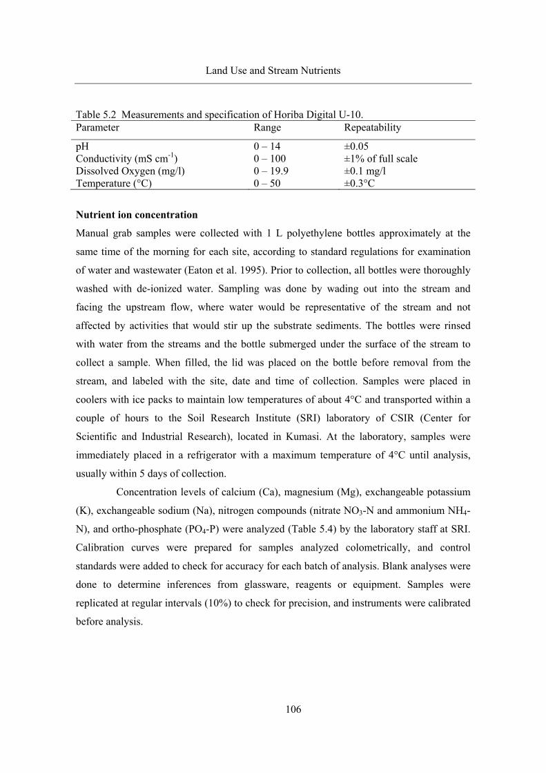
Land Use and Stream Nutrients

106

Table 5.2 Measurements and specification of Horiba Digital U-10. Parameter Range Repeatability

pH 0 – 14 ±0.05 Conductivity (mS cm-1) 0 – 100 ±1% of full scale Dissolved Oxygen (mg/l) 0 – 19.9 ±0.1 mg/l Temperature (°C) 0 – 50 ±0.3°C

Nutrient ion concentration

Manual grab samples were collected with 1 L polyethylene bottles approximately at the

same time of the morning for each site, according to standard regulations for examination

of water and wastewater (Eaton et al. 1995). Prior to collection, all bottles were thoroughly

washed with de-ionized water. Sampling was done by wading out into the stream and

facing the upstream flow, where water would be representative of the stream and not

affected by activities that would stir up the substrate sediments. The bottles were rinsed

with water from the streams and the bottle submerged under the surface of the stream to

collect a sample. When filled, the lid was placed on the bottle before removal from the

stream, and labeled with the site, date and time of collection. Samples were placed in

coolers with ice packs to maintain low temperatures of about 4°C and transported within a

couple of hours to the Soil Research Institute (SRI) laboratory of CSIR (Center for

Scientific and Industrial Research), located in Kumasi. At the laboratory, samples were

immediately placed in a refrigerator with a maximum temperature of 4°C until analysis,

usually within 5 days of collection.

Concentration levels of calcium (Ca), magnesium (Mg), exchangeable potassium

(K), exchangeable sodium (Na), nitrogen compounds (nitrate NO3-N and ammonium NH4-

N), and ortho-phosphate (PO4-P) were analyzed (Table 5.4) by the laboratory staff at SRI.

Calibration curves were prepared for samples analyzed colometrically, and control

standards were added to check for accuracy for each batch of analysis. Blank analyses were

done to determine inferences from glassware, reagents or equipment. Samples were

replicated at regular intervals (10%) to check for precision, and instruments were calibrated

before analysis.

Land Use and Stream Nutrients

107

Table 5.4 Methodology and apparatus used for testing for each nutrient parameter Parameter Apparatus/Method Reference

Ammonia nitrogen (NH4-N) Bertholot Colorimetric method Eaton et al., 1995

Nitrate nitrogen (NO3-N) Colorimetric Determination method

Cataldo et al, 1975

Exchangeable potassium (K)

Exchangeable sodium (Na)

Gallenkamp Flame Analyzer Model FGA-330 Eaton et al., 1995

Orthophosphate (PO4-P) Phosphorus-Molybdenium Blue method

Eaton et al., 1995

Calcium (Ca) EDTA Titrimetric method Eaton et al., 1995 Magnesium (Mg)

5.3 Data Analysis

5.3.1 Hydrology

In order to accurately assess the nutrient yields from each catchment, it is important to

estimate the stream discharge. Miscalculation of the discharge leads to errors in

determining nutrient loads, as this is the function of the amount of water that leaves the

catchment. To assess discharge as a proportion of total rainfall volume, the basic water

balance of each catchment system was established by the mass balance equation (Equation

5.1) (Shahin 2002):

( ) ( ) ( ) ETGWPSMDROPI re +±∆±+=+ (5.1)

Where: I = inflow to the system (e.g., irrigation), Pe = effective precipitation, O = outflow from the system, DR = drainage, ∆SM = change to soil moisture in storage, (GWP)r = groundwater discharge, and ET = evapotranspiration.

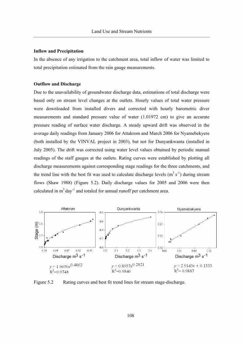
Land Use and Stream Nutrients

108

Inflow and Precipitation

In the absence of any irrigation to the catchment area, total inflow of water was limited to

total precipitation estimated from the rain gauge measurements.

Outflow and Discharge

Due to the unavailability of groundwater discharge data, estimations of total discharge were

based only on stream level changes at the outlets. Hourly values of total water pressure

were downloaded from installed divers and corrected with hourly barometric diver

measurements and standard pressure value of water (1.01972 cm) to give an accurate

pressure reading of surface water discharge. A steady upward drift was observed in the

average daily readings from January 2006 for Attakrom and March 2006 for Nyamebekyere

(both installed by the VINVAL project in 2003), but not for Dunyankwanta (installed in

July 2005). The drift was corrected using water level values obtained by periodic manual

readings of the staff gauges at the outlets. Rating curves were established by plotting all

discharge measurements against corresponding stage readings for the three catchments, and

the trend line with the best fit was used to calculate discharge levels (m3 s-1) during stream

flows (Shaw 1988) (Figure 5.2). Daily discharge values for 2005 and 2006 were then

calculated in m3 day-1 and totaled for annual runoff per catchment area.

Figure 5.2 Rating curves and best fit trend lines for stream stage-discharge.

Land Use and Stream Nutrients

109

Soil water storage

In calculating the changes in soil water storage (∆S), an estimate of the soil’s ability to

store water is required. The available water holding capacity of a soil is based on the

difference between its upper limits, i.e., field capacity (water content of soil at equilibrium),

and lower limits, i.e., permanent wilting point (when plants begin to wilt). Since soil

storage capacity and the initial soil moisture were unknown for the catchments, a balancing

routine was used to set the initial soil moisture at the beginning of each year to 0. This

assumes that there are no changes in major seasonal patterns from one year to the other and

annual soil moisture storage is 0 at the start of each year (Dr. C. Rodgers, personal

communication).

Evapotranspiration

In hydrological studies, evapotranspiration is generally calculated as the amount of

available water after discharge and soil storage changes; in physical meteorology, it is the

combined process of both evaporation from soil and plant surfaces and transpiration

through the stomata of the plant surfaces (Shahin 2002). Potential evapotranspiration is the

rate at which water is removed from the soil surface by evapotranspiration if there is no

restriction on the available water. Actual evapotranspiration is the actual amount for a

specified crop at a designated time, corrected for the possible condition of dry soil.

To determine the evaporative capacity of the atmosphere for the study area, the

FAO Penman-Monteith equation (Equation 5.2) was used to calculate ETo, i.e., or the

reference crop evapotranspiration. This equation estimates evaporation of a hypothetical

crop with an assumed height of 0.12 m, a fixed surface resistance of 70 sm-1 and an albedo

of 0.23, and is recommended as the standard method for best results and minimum possible

errors (Allen et al. 1998).

Land Use and Stream Nutrients

110

( ) ( )( )2

2

34.01273

900408.0

u

eeuT

GRET

asn

o ++∆

−+

+−∆=

γ

γ (5.2)

Where: ETo = reference evapotranspiration [mm day-1], Rn = net radiation at the crop surface [MJ m-2 day-1], G = soil heat flux density [MJ m-2 day-1], T = mean daily air temperature (at 2 m) [°C], u2 = wind speed at 2 m height [m s-1], (es - ea) = saturation vapor pressure deficit [kPa], ∆ = slope vapor pressure curve [kPa°C-1], and γ = psychrometric constant [kPa°C-1]. ETo values were calculated using an Excel spreadsheet.

Climatic parameters required for ETo computation include solar radiation, air

temperature, air humidity and wind speed, which were all obtained from the VINVAL

weather station. Missing data due to infrequent downloading and malfunctioning sensors

for rainfall and humidity in 2006, were estimated using data obtained from the installed

barometer at Duyankwanta, correlations with the regional weather station data (Kumasi), or

calculation procedures recommended by the FAO guidelines for missing or unreliable data

(Allen et al. 1998).

Temperature

For missing air temperature values (12 March to 22 May 2005; 29 October 2005 to 15

September 2006) from the VINVAL weather station, a linear correlation with average daily

temperature data from the weather station and the barometer installed in the same

catchment showed a regression coefficient of R2 = 0.7951 (Figure 5.3). The formula

obtained was used to fill in for the missing data.

Land Use and Stream Nutrients

111

Figure 5.3 Graph and linear correlation between average temperature values obtained

from the Barometer diver and VINVAL weather station. Humidity

In estimating actual vapor pressure (Eaton et al. 1995), the FAO guidelines recommend

using both maximum and minimum values of relative humidity (Equation 5.3).

2100

)(100

)( minmax

maxmin

RHTe

RHTe

e

oo

a

+= (5.3)

Where: ea = actual vapour pressure [kPa], eo (Tmin) = saturation vapour pressure at daily minimum temperature [kPa], eo (Tmax) = saturation vapour pressure at daily maximum temperature [kPa], RHmax = maximum relative humidity [%], and RHmin = minimum relative humidity [%]

The VINVAL weather station humidity sensors malfunctioned for most of 2006. The RH

data of the meteorological department were substituted for the determination of ETo for the

catchments. Since the evaporative capacity of the atmosphere is estimated, variations due to

vegetative cover is not reflected in the results obtained. In addition, since RHmin values for

Land Use and Stream Nutrients

112

July 2006 were missing for the Kumasi meteorological station, FAO’s suggestion for the

estimation of ea when RHmin readings are uncertain (Equation 5.4), was applied.

100)( max

minRH

Tee oa = (5.4)

Wind

FAO’s recommendation is to use 2.0 m s-1 as the average wind speed for missing wind data.

However, an average value of 0.5 m s-1 was used for the catchment areas, which is more

representative of the wind speeds observed from available data from both VINVAL and

Kumasi weather stations (Figure 5.4).

Figure 5.4 Average daily wind speeds (m s-1) from Kumasi and VINVAL weather

stations.

5.3.2 Stream chemistry

Box and whisker plots show the range of all measured concentrations for each catchment

for the entire period; 50% of the data points lies within the box, with the middle horizontal

Land Use and Stream Nutrients

113

line of the box representing the median value, whiskers showing the range of data, and

circles showing the outliers.

Flow-weighted mean ion concentrations

To determine the overall average concentration of nutrient ions for a time period in order to

enable comparisons between catchments, each sample’s contribution with respect to

discharge needs to be accurately estimated. The discharge volume for each sample varies

from one measurement to another, and as such each sample has to be weighted differently

when averages are calculated. Data on the measured concentration (Ci) are weighted by the

sample-time window (ti) and discharge at the time of sampling (Qi). The flow weighted

mean concentration (FWMC) represents the total load for the time period (month, season

and year) divided by the total discharge for the time period (Equation 5.5).

∑

∑

⋅

⋅⋅= n

ii

n

iii

Qt

QtCFWMC

1

1

)(

)( (5.5)

5.3.3 Nutrient load estimation

Ideally, with continuous discharge and concentration data, the actual load of pollutants

transported through the cross section of a river or stream during a time interval (Equation

5.6) is usually expressed as:

∫=2

1

)()(t

t

dttCtQL (5.6)

Where: L represents the load between time t1 and t2, Q(t) the stream flow at time t, and C(t) the chemical concentration at time t.

With C not provided as a continuous measurement (one sample approximately

every 48 hours as compared to the hourly data available for stream flow), the annual

Land Use and Stream Nutrients

114

nutrient load from the catchments was calculated by two different methods – the averaging

or interpolation method and the ratio estimation method. The averaging method includes

commonly used calculations shown below (Littlewood et al. 1998; Letcher et al. 2002; Li et

al. 2003; Quilbé et al. 2006; Johnes 2007) (Equations 5.7 and 5.8).

(i) Average sample concentration times average sample discharge:

QCnQnd

Cnd

nLn

ii

n

ii ⋅⋅=⎟

⎠

⎞⎜⎝

⎛⎟⎠

⎞⎜⎝

⎛= ∑∑

== 111

11 (5.7)

Where: n is the total number of days for the period of load estimation, nd the number of days in the period that concentration data was measured, Ci is the sampled concentration on day i, and Qi the average flow on day i.

(ii) Average concentration (Dann et al. 1986) or mean concentration times annual

discharge

q

n

ii

nd

CL µ⋅=

∑=1

2 (5.8)

Where: µq is mean daily flow for the statistical period. The comparison of annual estimates obtained from Equations 5.7 and 5.8 yielded the same values, so only L2 was used for comparison with the equation presented below.

(iii) Flow-weighted average sample concentration times average sample discharge

(Equation 5.9):

qn

ii

n

iii

FW

Q

QCKL µ∑

∑

=

==

1

1 (5.9)

Land Use and Stream Nutrients

115

The ratio estimator method includes the Beale’s Ratio estimator (Beale 1962) as reported

by Quilbé et al. (2006), which multiplies LFW in Equation 5.9 by a ratio that accounts for

the covariance between load and stream flow values (Equation 5.10). This method has

shown the least biased estimates and inaccuracy in the comparison of estimation methods to

the ‘true load’ (i.e., comparison of nutrient estimation of artificial reduced data to t hat of

the full dataset), especially in cases where there is relatively sparse concentration data and

an absence of strong correlation between concentration and flow data (Preston et al. 1989;

Mukhopadhyay and Smith 2000; Letcher et al. 2002; Endreny and Hassett 2005; Quilbé et

al. 2006; Johnes 2007).

A third method, the Regression Method, has worked well in other studies

(Endreny and Hassett 2005; Johnes 2007). However, for this method, a linear correlation

relationship must first be established between concentration and discharge levels for

nutrients. In addition, a calibration period of at least 75 samples taken over a two-year

period, with 50% during low flow and 50% during high flows, is needed to establish a

reliable linear relationship (Richards 2000). Correlation values higher than a threshold

value of 0.5 has been suggested for the coefficient of determination (r2) before the

regression method can be used, meaning that more than 50% of the variability of

concentration should be explained by the stream flow (Quilbé et al. 2006). For this study,

correlations between nutrients and discharge for the three catchments were all lower than

the r2 = 0.5 screening method suggested (Table 5.4). Since the regression method was not

applicable, the Beale estimator, also a reliable method, was used for estimating nutrient

loads. The annual mean estimates calculated by the averaging methods are presented in the

results only for comparative purposes, with seasonal and monthly values based solely on

the Beale’s ratio method.

The Beale method weights the concentration values by adjusting the mean of daily

loads (i.e., product of concentration and discharge on days when samples are taken) by a

flow ratio (Equation 5.10). This ratio is obtained by dividing the average flow for the

period by the average flow for the days on which samples were obtained. A bias correction

factor is also included in the calculation to compensate for the effects of correlation

between discharge and load. The ratio method assumes increase in concentration with

Land Use and Stream Nutrients

116

increases in flow – a factor which is prominent in small streams and rivers where increased

concentration occurs mostly during storm runoff.

⎟⎟⎟⎟⎟

⎠

⎞

⎜⎜⎜⎜⎜

⎝

⎛

⋅+

⋅⋅+

⋅=

2

' 11

11

Q

Snd

QCQS

ndQ

CQLQ

CQ

qsBeale

µ (5.10)

The parameter SCQ (Equation 5.11) is a modified covariance of the flow and load

and is calculated by:

⎟⎠

⎞⎜⎝

⎛ −−

= ∑=

n

iiiCQ CQQndQC

ndS

111

(5.11)

QS (Equation 5.12) represents a sample variance on the daily flows for sample

size nd and is given by

⎟⎠

⎞⎜⎝

⎛ −−

= ∑=

n

iiQ

QndQnd

S1

22

11

(5.12)

Data was processed to ensure consistency of units, and all concentration units

were converted to milligrams per liter (mg L-1) and discharge units expressed in m3 day-1.

Unit conversions were performed throughout all load calculations to ensure that final loads

were consistently reported in the standard units of kilograms per specified period, i.e., day,

month, season and year.

Land Use and Stream Nutrients

117

Table 5.4 Correlation values (r2) between nutrient concentrations and discharge mg L-1 Attakrom Dunyankwanta Nyamebekyere

Ca 0.10 0.02 0.03K 0.07 0.07 0.01Mg 0.05 0.02 0.00Na 0.07 0.01 0.03NH4-N 0.01 0.00 0.00NO3-N 0.01 0.02 0.05PO4-P 0.00 0.06 0.13

Nutrient yield

In order to assess and compare the pollutant loads from the different catchments, which are

different in size, the pollutant load per unit area, or pollutant yield, was also calculated

(Equation 5.13). This yield normalizes the load of the monitored catchment area allowing

for more relative comparisons to be made between different land-use intensities. Yield, Y

(kg ha-1 yr-1), was obtained by dividing the total pollutant load, L (kg) for a given time

period by the catchment area A (ha).

ALY = (5.13)

5.3.4 Statistical tests

Statistical tests were carried out only for detection of the differences in spatial trends and

not for testing if these differences were significant enough to impact the aquatic system,

although general comparisons are made to established WRC water quality standards for

aquatic ecosystem health and domestic users. A significance level, or α-value, of 5% (0.05)

was used for all comparisons, although it is important to note that significant differences

are not always environmentally consequential. The null hypothesis (H0) is that there are no

differences in nutrient concentrations between catchments for different land-use intensities.

H0 is rejected when p values are less than or equal to the α-value (p<0.05), assuming that

there are significant differences between the catchments. When p>0.05, it is assumed that

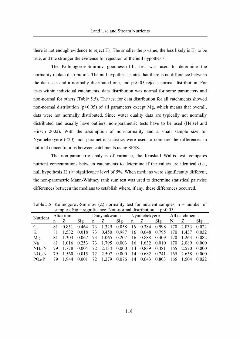
Land Use and Stream Nutrients

118

there is not enough evidence to reject H0. The smaller the p value, the less likely is H0 to be

true, and the stronger the evidence for rejection of the null hypothesis.

The Kolmogorov-Smirnov goodness-of-fit test was used to determine the

normality in data distribution. The null hypothesis states that there is no difference between

the data sets and a normally distributed one, and p<0.05 rejects normal distribution. For

tests within individual catchments, data distribution was normal for some parameters and

non-normal for others (Table 5.5). The test for data distribution for all catchments showed

non-normal distribution (p<0.05) of all parameters except Mg, which means that overall,

data were not normally distributed. Since water quality data are typically not normally

distributed and usually have outliers, non-parametric tests have to be used (Helsel and

Hirsch 2002). With the assumption of non-normality and a small sample size for

Nyamebekyere (<20), non-parametric statistics were used to compare the differences in

nutrient concentrations between catchments using SPSS.

The non-parametric analysis of variance, the Kruskall Wallis test, compares

nutrient concentrations between catchments to determine if the values are identical (i.e.,

null hypothesis H0) at significance level of 5%. When medians were significantly different,

the non-parametric Mann-Whitney rank sum test was used to determine statistical pairwise

differences between the medians to establish where, if any, these differences occurred.

Table 5.5 Kolmogorov-Smirnov (Z) normality test for nutrient samples, n = number of samples, Sig = significance. Non-normal distribution at p<0.05

Nutrient Attakrom Dunyankwanta Nyamebekyere All catchments n Z Sig n Z Sig n Z Sig N Z Sig

Ca 81 0.851 0.464 73 1.329 0.058 16 0.384 0.998 170 2.033 0.022K 81 1.532 0.018 73 0.450 0.987 16 0.648 0.795 170 1.437 0.032Mg 81 1.303 0.067 73 1.065 0.207 16 0.888 0.409 170 1.263 0.082Na 81 1.016 0.253 73 1.795 0.003 16 1.632 0.010 170 2.089 0.000NH4-N 79 1.778 0.004 72 2.134 0.000 14 0.839 0.481 165 2.570 0.000NO3-N 79 1.560 0.015 72 2.507 0.000 14 0.682 0.741 165 2.638 0.000PO4-P 79 1.944 0.001 72 1.279 0.076 14 0.643 0.803 165 1.504 0.022

Land Use and Stream Nutrients

119

5.4 Results and Discussion

5.4.1 Annual dynamics

Hydrology

In the comparison and analysis of nutrient levels and yields for streams, the accuracy of

stream-flow runoff has been determined to be the single most important factor (e.g., Li et

al. 2003; Aulenbach and Hooper 2005; Johnes 2007). The precision of discharge

measurements is, therefore, critical for the appropriate estimation of loads, especially for

small ephemeral streams. Ideally, this accuracy should be supported by more efficient

hydrological background studies, which have not been specifically established for the

catchments in this study. However, inferences are drawn from or compared to various

hydrological studies carried out by the GLOWA project, which have investigated issues

such as rates of surface runoff and infiltration, the impact of climate variability on

hydrology, and tree-water use and evapotranspiration rates within the Volta Basin (Ajayi

2004; Oguntunde 2004; Jung 2006). Although climatic data are available for 2005 and

2006, stream discharge readings for the three catchments began in the minor rainy season

of September 2005. Without any detailed and long-term background hydrological data, an

approximation of evapotranspiration for each catchment was calculated as total water

volume input and output for only 2006 (Table 5.6), as data available for 2005 is partial.

From September to December 2006, the diver datalogger for Nyamebekyere malfunctioned

and measurements for this period were limited to periodic gauge readings.

For 2006, precipitation ranged between 1010.4 mm yr-1 (in Attakrom) and 1679.6

mm yr-1 (in Nyamebekyere), which indicates a large variability between catchments.

Precise estimates of the volume of areal precipitation generally require measurements by

rain gauges at several points within the catchment, since one gauge usually represents an

area of 150 cm2 (Shaw 1988) and can be a source of errors for larger scale estimations. In

addition, the rain gauges were read by non-scientific staff, which could lead to instances of

misreading or unrecorded events. However, in a study modeling the climate years 1936-

1961 for the Volta Basin, results for the south-western parts showed an annual average

precipitation value of 1800 mm, with a large range between 1340 mm and 2175 mm,

similar to that estimated for the catchments (Oguntunde 2004).

Land Use and Stream Nutrients

120

Although discharge volumes varied between catchments, the percentage runoff was similar

for Attakrom (2.3%) and Nyamebekyere (2.5%, but with missing data estimated by manual

gauge readings), but much higher in Dunyankwanta (6.2%). Studies comparing rainfall-

runoff percentages at plot levels in parts of the Volta Basin estimated a 5% runoff fraction

for long runoff plots (2 m x 18 m), and higher discharge fractions of 33% for smaller plots

(2m x 2m) (Ajayi 2004). In the Volta Basin, the average fraction of rainfall which becomes

river discharge is estimated at 9%, although values range for different locations from 4.9%

in the Black Volta, which lies adjacent to the catchment sites, to higher values of 13.5% in

the more northern Oti due to its steeper terrains (Andreini et al. 2000). Despite the

differences between catchments, the fraction of rainfall which became stream discharge in

this study is comparable to the research of Andreini et al. (2000) and Ajayi (2004). The

conversion of land from forested areas to agricultural lands often leads to significant

increases in runoff volumes due to lower infiltration and evapotranspiration rates

(Siriwardena et al. 2006; Li et al. 2007). The estimated lower discharge volumes in

Nyamebekyere, although with the highest precipitation values, may therefore be indicative

of higher evapotranspiration and infiltration typical of the greater vegetation cover of

forested areas (Ajayi 2004; Oguntunde 2004).

To assess the effects of land-use intensity on soil properties in the catchments, soil

compaction was assessed by evaluating soil bulk density, pore size class distribution and

soil water retention parameters (Ungaro et al. 2004). Overall, the soils of the three

catchments are dominated by loams (36%) followed by sandy loams, clays and clay loams

(12% each). A positive trend was observed in bulk density average values with increasing

land-use intensity, although the differences were not statistically significant. The positive

trend in bulk density was correlated to an increase in microporosity (pore Ø< 7.5 µm) and a

decrease in macroporosity (pore Ø>100 µm). Statistical differences were found in

microporosity only between medium and high land-use intensity catchments, and in

macroporosity between (i) low and high land-use intensity, and (ii) medium and high land-

use intensity. A positive trend in soil water retention parameters was also observed with

increasing land-use intensity, although differences were significant only between the low

and high land-use intensity catchments. There are indications that increasing land-use

Land Use and Stream Nutrients

121

intensity influences water retention properties. However, without detailed studies on how

the vertical variability of the soils, hydraulic properties, dominant flow paths, etc. influence

discharge rates, conclusive statements cannot be made about the changes in water yield as

natural land is converted to agricultural land.

Rates of evapotranspiration can be measured and/or estimated from models or

empirical approaches. Direct measurement approaches (e.g., using lysimeters) are difficult

and time-consuming. In models, various parameters which interact to influence

evapotranspiration are incorporated, i.e., weather (radiation, air temperature, humidity,

wind speed), crop factors (crop type, variety and development stage), and environmental

conditions (soil salinity, fertility, diseases, pests, poor soil management, ground cover,

plant density and soil water content) (Oguntunde 2004). Meteorological data was rather

used for this study, as it is also effective at estimating evapotranspiration with improved

frequency and accuracy (Shahin 2002). Potential evapotranspiration values for the south-

western parts of the Volta Basin, seen on evapotranspiration maps created by the

Advection-Aridity (AA) model for 25-year data series (1936-1961) (Oguntunde 2004),

were between 1340 and 1433 mm, and comparable to this study’s estimated ETo (1396.3).

The AA model also shows ETa values between 1297 and 1353 mm annually for the

catchment areas ranges, which is higher than values estimated for Attakrom (987.5 mm),

and lower than that of Nyamebekyere (1638.3 mm, a value that may be biased due to

missing data). This could be due to the variations in surface albedo as a result of land-use

intensity. Surface albedo is a major factor influencing the amount of water available for

evapotranspiration depending on the type of vegetation, with as much as 1492 mm per

annum for land-use comprised of mixed forest, mixed dry/irrigated crops, and crop/wood

mosaic (Oguntunde 2004).

From the above discussions, precipitation values (although with high variation),

discharge estimates (although Nyamebekyere with missing data) and calculated

evapotranspiration rates using meteorological data, are similar to estimates obtained by

other researchers within the study basin. With no supporting hydrological data on how

land-use affects water dynamics from precipitation to surface runoff in small catchments,

these estimates are adequate for the objectives of calculating nutrient load exports.

Land Use and Stream Nutrients

122

Table 5.6 Total precipitation (P), total discharge (Q), discharge as % precipitation, actual evapotranspiration (ETa), potential evapotranspiration (ET0) - 2006

Catchment Total P (mm yr-1)

Total Q (mm yr-1)

Q as % P Total ETa (mm yr-1)

Total ET0 (mm yr-1)

Attakrom 1010.4 22.9 2.3 987.5

1396.3Dunyankwanta 1286.5 79.9 6.2 1206.6

Nyamebekyere 1679.6 41.3* 2.5 1638.3 * Total discharge may be underestimated with only manual gauge readings from Sep to Dec 2006

Chemical State (C)

In order to assess the quality of the streams from the three catchments, measured values for

physico-chemistry and nutrient ion concentrations (Appendix 5) are compared to the Raw

Water Quality Criteria and Guidelines for Ghanaian freshwaters (WRC 2003a). These

standards have been set for specific uses of freshwater in Ghana (such as domestic,

recreational, industrial, agricultural, aquaculture, and for the protection of the aquatic

environment) and establish the specific limits within which nutrient concentrations should

be maintained, i.e., a Target Water Quality Range (TWQR) which is the range of ideal

nutrient concentrations. This ideal range, or the ‘No Effect Range’, means that there are no

adverse effects on the quality of water for a particular use or on aquatic ecosystem health.

For the purpose of this study, the guidelines set for domestic water use (WRC 2003e), i.e.,

for washing, cooking, bathing, drinking, etc., and aquatic ecosystem health (WRC 2003f)

are used (Table 5.7). For those parameters without set guidelines, references from other

literature are used.

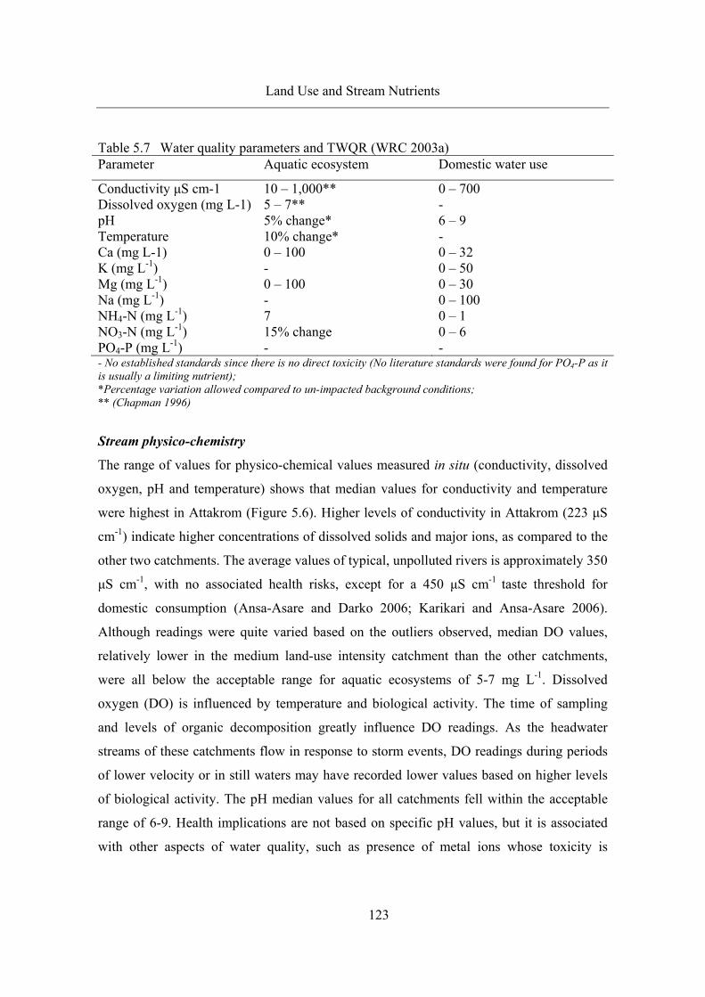
Land Use and Stream Nutrients

123

Table 5.7 Water quality parameters and TWQR (WRC 2003a) Parameter Aquatic ecosystem Domestic water use

Conductivity µS cm-1 10 – 1,000** 0 – 700 Dissolved oxygen (mg L-1) 5 – 7** - pH 5% change* 6 – 9 Temperature 10% change* - Ca (mg L-1) 0 – 100 0 – 32 K (mg L-1) - 0 – 50 Mg (mg L-1) 0 – 100 0 – 30 Na (mg L-1) - 0 – 100 NH4-N (mg L-1) 7 0 – 1 NO3-N (mg L-1) 15% change 0 – 6 PO4-P (mg L-1) - - - No established standards since there is no direct toxicity (No literature standards were found for PO4-P as it is usually a limiting nutrient); *Percentage variation allowed compared to un-impacted background conditions; ** (Chapman 1996)

Stream physico-chemistry

The range of values for physico-chemical values measured in situ (conductivity, dissolved

oxygen, pH and temperature) shows that median values for conductivity and temperature

were highest in Attakrom (Figure 5.6). Higher levels of conductivity in Attakrom (223 µS

cm-1) indicate higher concentrations of dissolved solids and major ions, as compared to the

other two catchments. The average values of typical, unpolluted rivers is approximately 350

µS cm-1, with no associated health risks, except for a 450 µS cm-1 taste threshold for

domestic consumption (Ansa-Asare and Darko 2006; Karikari and Ansa-Asare 2006).

Although readings were quite varied based on the outliers observed, median DO values,

relatively lower in the medium land-use intensity catchment than the other catchments,

were all below the acceptable range for aquatic ecosystems of 5-7 mg L-1. Dissolved

oxygen (DO) is influenced by temperature and biological activity. The time of sampling

and levels of organic decomposition greatly influence DO readings. As the headwater

streams of these catchments flow in response to storm events, DO readings during periods

of lower velocity or in still waters may have recorded lower values based on higher levels

of biological activity. The pH median values for all catchments fell within the acceptable

range of 6-9. Health implications are not based on specific pH values, but it is associated

with other aspects of water quality, such as presence of metal ions whose toxicity is

Land Use and Stream Nutrients

124

influenced by pH levels (WRC 2003e). The pH of surface- and groundwater usually reflects

their humic acids CO2, −23CO and −

3HCO contents. Temperature values are important due to

its effect on other physical phenomena such as rate of biochemical and chemical reactions

in the water body, reduction in solubility of gases and amplifications of taste and odor

(Olajire and Imeokparia 2001). In forested areas, canopies provide shade that maintains the

low stream temperatures that are typical of these catchments, which was also observed in

Nyamebekyere. Results of the Kruskal Wallis test indicate that there is enough evidence of

differences between the catchments at a significance level of 5% (Table 5.8) for

conductivity, dissolved oxygen, and temperature.

Figure 5.5 Box and whisker plots showing range of measurements for conductivity,

DO, pH, and temperature (September 2005-December 2006). Dotted line represents the mean value, solid line represents the median value, and numbers at the bottom represent number of total samples.

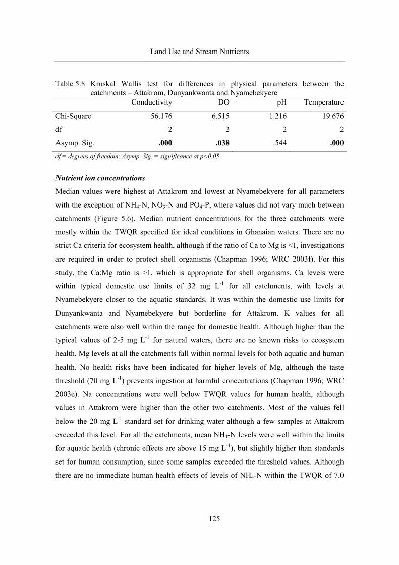
Land Use and Stream Nutrients

125

Table 5.8 Kruskal Wallis test for differences in physical parameters between the catchments – Attakrom, Dunyankwanta and Nyamebekyere

Conductivity DO pH Temperature

Chi-Square 56.176 6.515 1.216 19.676

df 2 2 2 2

Asymp. Sig. .000 .038 .544 .000df = degrees of freedom; Asymp. Sig. = significance at p<0.05

Nutrient ion concentrations

Median values were highest at Attakrom and lowest at Nyamebekyere for all parameters

with the exception of NH4-N, NO3-N and PO4-P, where values did not vary much between

catchments (Figure 5.6). Median nutrient concentrations for the three catchments were

mostly within the TWQR specified for ideal conditions in Ghanaian waters. There are no

strict Ca criteria for ecosystem health, although if the ratio of Ca to Mg is <1, investigations

are required in order to protect shell organisms (Chapman 1996; WRC 2003f). For this

study, the Ca:Mg ratio is >1, which is appropriate for shell organisms. Ca levels were

within typical domestic use limits of 32 mg L-1 for all catchments, with levels at

Nyamebekyere closer to the aquatic standards. It was within the domestic use limits for

Dunyankwanta and Nyamebekyere but borderline for Attakrom. K values for all

catchments were also well within the range for domestic health. Although higher than the

typical values of 2-5 mg L-1 for natural waters, there are no known risks to ecosystem

health. Mg levels at all the catchments fall within normal levels for both aquatic and human

health. No health risks have been indicated for higher levels of Mg, although the taste

threshold (70 mg L-1) prevents ingestion at harmful concentrations (Chapman 1996; WRC

2003e). Na concentrations were well below TWQR values for human health, although

values in Attakrom were higher than the other two catchments. Most of the values fell

below the 20 mg L-1 standard set for drinking water although a few samples at Attakrom

exceeded this level. For all the catchments, mean NH4-N levels were well within the limits

for aquatic health (chronic effects are above 15 mg L-1), but slightly higher than standards

set for human consumption, since some samples exceeded the threshold values. Although

there are no immediate human health effects of levels of NH4-N within the TWQR of 7.0

Land Use and Stream Nutrients

126

mg L-1 for aquatic ecosystems, taste and odor complaints may occur at concentrations

above 1.5 mg L-1. For NO3-N levels, mean and median concentrations were comparable to

the typical concentrations of natural surface waters (5 mg L-1), although many of the

outliers exceeded this for Attakrom and Dunyankwanta. High concentrations above 10.0

mg L-1 can be potentially toxic to human health, as excessive nitrate may result in infant

cyanosis, also known as methemoglobinemia (which interferes with the oxygen carrying

capacity of the blood) or ‘blue baby syndrome’, in children less than one year old

(Carpenter et al. 1998; WRC 2003e). There are no significant health risks for older children

or adults, and boiling water will not remove nitrate. Nitrate can also be toxic to livestock if

reduced to nitrite, and levels of 40-100 mg L-1 in drinking water is considered risky. For

PO4-P, there are no established drinking water standards since it is not considered to be

directly toxic to humans and animals, but can be toxic to aquatic life as a result of

stimulated productivity and increased eutrophication (Carpenter et al. 1998).

Nutrient concentrations were flow weighted over time periods, i.e., adjusted to

discharge levels at sampling time in order to normalize the concentration values for average

discharge, for comparison at varying discharge levels. Concentrations differ between for

Ca, Mg, Na and NO3-N, with lower variations for K, NH4-N and PO4-P. Attakrom showed

the highest flow-weighted concentrations, similar to the median values, with the exception

of K and NH4-N (highest in Dunyankwanta) and NO3-N ( highest in Nyamebekyere). The

dominance in ionic composition for each catchment stream follows the order typical for

natural freshwater systems in Ghana, i.e., Ca>Mg>Na (K) (Chapman 1996; WRC 2003f).

Results of the Kruskal Wallis test show that at a significance level of 5% there are

differences between catchments for all stream nutrient concentrations except NH4-N and

NO3-N (Table 5.9). At p<0.05, the Mann Whitney test results (Table 5.10) show that the

distinctions between Attakrom and Dunyankwanta are based on significant differences in

the measured concentrations of the cations – Ca, Mg, Na and K. Between Attakrom and

Nyamebekyere, differences are significant for all parameters except the nitrogen

compounds; and between Dunyankwanta and Nyamebekyere, differences are significant for

Ca, Mg, Na and PO4-P.

Land Use and Stream Nutrients

127

Since water interacts with the soils before entering streams, nutrient concentrations can be

influenced by the soil properties. The VINVAL project’s soil characterization for the three

study catchments (Ungaro et al. 2004) provides soil quality assessment in terms of

percentage organic carbon. Results showed significant differences in the mean percentage

organic carbon content of the topsoil. Dunyankwanta had the highest amount of organic

carbon (3.14%) compared to Attakrom (2.24%) and Nyamebekyere (1.76%). In order to

compare the soils, the authors based their comparisons on soil organic matter stratification,

which is defined as a property at the soil surface divided by the same property at a lower

depth. A high rate for organic carbon generally indicates relatively undisturbed soil. The

authors found significant differences (p<0.05) between the three catchments, with

Nyamebekyere having the lowest stratification ratio (0.50), followed by Attakrom (1.85),

and the highest ratio in Dunyankwanta (3.04). With no observed correlations between the

carbon levels and soil texture (silt + clay), the VINVAL report proposed that this could be

due to the fact that storage of carbon in forest biomass results in lower levels in the soils of

forests. The report also suggests that a higher proportion of plant residue in grassland

vegetation is of root matter, which decomposes slowly and contributes more efficiently to

soil humus formation than forest leaf litter. However, detailed information on the history

and duration of cultivation, soil formation and organic carbon cycles are required to

properly assess differences between catchments. In neighboring inland valley watersheds, a

study investigating soil properties under different land uses showed that mean nitrogen

contents was high, possibly due to the dense vegetative cover, litter fall and higher

mineralization (Annan-Afful et al. 2005). Contrary to the VINVAL report, the study

suggests that soils under permanent vegetation (such as primary forests) or cropping

systems (cocoa farms) generally have a high organic carbon content. This means that these

systems may be more effective in restoring soil organic matter than in systems where

annual plants were grown. During the soil drying phases in the dry season, reduced forms

of nitrogen, particularly NH4+, are nitrified to NO3

- that may be lost by leaching during the

rains. Phosphorus is low in these areas possibly due to P-fixing compounds in the soil.

These studies confirm that natural background levels of soil nitrogen are generally high and

phosphorus are low, which was observed for the catchments.

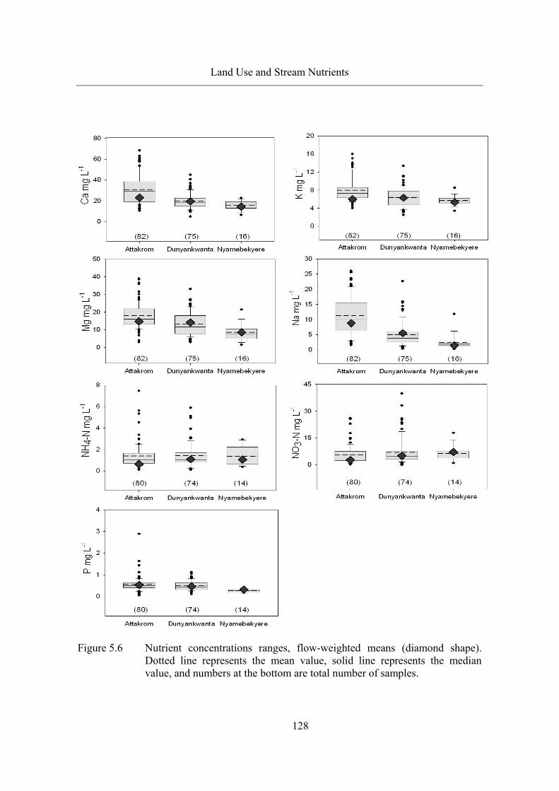
Land Use and Stream Nutrients

128

Figure 5.6 Nutrient concentrations ranges, flow-weighted means (diamond shape).

Dotted line represents the mean value, solid line represents the median value, and numbers at the bottom are total number of samples.

Land Use and Stream Nutrients

129

Table 5.9 Kruskal Wallis Test for differences in nutrient parameters between the catchments - Attakrom, Dunyankwanta and Nyamebekyere.

Ca K Mg Na NH4-N NO3-N PO4-P

Chi-Square 38.922 20.333 31.233 57.173 .103 2.023 20.914df 2 2 2 2 2 2 2Asymp. Sig. .000 .000 .000 .000 .950 .364 .000

df = degrees of freedom; Asymp. Sig. = significance at p<0.05

Table 5.10 Mann Whitney tests for differences in nutrient parameters between Attakrom, Dunyankwanta and Nyamebekyere (Sig. = significance at p<0.05)

a Grouping Variable: Catchment (Attakrom and Dunyankwanta) Ca K Mg Na NH4-N NO3-N PO4-P

Mann-Whitney 1438.000 1976.000 1789.500 1202.000 2800.000 2559.000 2562.000

Wilcoxon 4139.000 4677.000 4490.500 3903.000 5960.000 5719.000 5190.000Z -5.500 -3.548 -4.224 -6.349 -.164 -1.062 -1.051Sig. (2-tailed) .000 .000 .000 .000 .870 .288 .293

b Grouping Variable: Catchment (Attakrom and Nyamebekyere) Ca K Mg Na NH4-N NO3-N PO4-P

Mann-Whitney 172.500 217.500 141.500 69.500 535.000 448.000 146.500Wilcoxon 308.500 353.500 277.500 205.500 640.000 3608.000 251.500Z -4.625 -4.185 -4.925 -5.624 -.193 -1.128 -4.368Sig. (2-tailed) .000 .000 .000 .000 .847 .259 .000 c Grouping Variable: Catchment (Dunyankwanta and Nyamebekyere) Ca K Mg Na NH4-N NO3-N PO4-P

Mann-Whitney 396.500 455.500 325.000 200.000 475.500 441.500 147.000Wilcoxon 532.500 591.500 461.000 336.000 580.500 3069.500 252.000Z -2.007 -1.373 -2.769 -4.103 -.333 -.731 -4.178Sig. (2-tailed) .045 .170 .006 .000 .739 .465 .000

Nutrient load (P)

The mean annual nutrient load was calculated for 2006, as discharge and nutrient

measurements for 2005 were obtained from September and are therefore not representative

of the entire year. The contribution of nutrient loads for this period, which represents the

minor rainy season 2005 (September to December 2005), are assessed in the seasonal and

Land Use and Stream Nutrients

130

monthly loads sections. In the absence of more frequent data, the accuracy of the loads

estimated for the three catchments cannot be validated, especially as there are no available

published data on loads from small catchments as a function of a predominant type of land-

use. The comparison of load estimates to other countries have no real meaning, since

hydrological dynamics, soil properties and pollutant transport processes depend on the

characteristics of the catchment. However, since the purpose of this study was to compare

catchments with similar hydro-morphological characteristics, the load estimates obtained

are informative about the differences between the catchments based on their specific land-

use intensities.

From the results, the magnitude of total load of each nutrient exported from the

three catchments is in the order Dunyankwanta>Nyamebekyere>Attakrom (with the

exception of PO4-P where Attakrom values are higher than those for Nyamebekyere) (Table

5.11). Total annual nutrient loading from Dunyankwanta were higher than Attakrom and

Nyamebekyere. As discussed earlier (Section 5.3.3), Beale’s Ratio method is known to be

relatively more accurate and unbiased in nutrient load estimation, as it weights the

concentration values with discharge levels, and also provides a correction factor for the co-

variance between concentration and load. However, in order to assess the degree of

possible bias or inaccuracies that may result from the calculations, Quilbé et al. (2006)

suggest the comparison of different averaging procedures. The load estimations, obtained

using the equations for L2, LFW and LBeale’s presented in Section 5.3.3, are therefore

compared (Table 5.11). L2 estimates, i.e., values from the averaging calculation method

(un-weighted concentrations), are on average approximately 20% higher than Beale’s Ratio

estimator for the different nutrients, although Duyankwanta shows relatively less variation.

The mean annual load of PO4-P calculated for Nyamebekyere was lower than the Beale’s

estimate, indicating that averaging the sparsely available concentration data led to

underestimations when there were low values with low flow levels, whereas the flow-

weighted formulas adequately weighted the concentration with the flow. The Beale’s

method has performed well when tested in a number of catchments for the estimation of

nutrients and sediment loads, however, it has been noted that the influence of the correction

factor decreases as the number of samples increase (Webb et al. 2000; Johnes 2007). The

Land Use and Stream Nutrients

131

flow-weighted estimates, i.e., LFW, which is essentially minus the correction factor in the

Beale’s equation, confirms this as differences of less than 5% is observed for all nutrients at

all sites. The performance of the correction factor is thus not clear when results are tested

against full records. The sampling regime of every 48 hours, for this study, may have been

frequent enough to reduce the bias between the concentration and flow that usually occurs

with infrequent sampling; however, without any other background concentration or

discharge information for verification, this can only be a tentative conclusion.

Table 5.11 Annual nutrient loads (kg yr-1) for 2006 for the three catchments, calculated by Beale’s Ratio estimator method; and the mean relative difference (%) of load estimates calculated by equations L2 (Equation 5.8) and LFW (Equation 5.9).

Nutrient Attakrom Dunyankwanta Nyamebekyere Beale %L2 %LFW Beale %L2 %LFW Beale %L2 %LFW

Ca 2371.0 30.9 0.8 10669.1 7.9 3.7 3270.5 21.8 4.3K 705.2 24.0 0.8 2681.2 10.9 3.7 1201.8 10.0 4.3Mg 1887.0 16.4 0.8 6467.5 18.2 3.7 1905.7 20.5 4.3Na 917.7 36.9 0.8 2327.9 21.9 3.7 361.7 45.0 4.3NH4-N 157.1 9.8 0.7 744.8 13.5 3.8 343.3 21.7 2.6NO3-N 681.7 17.8 0.7 3021.1 19.9 3.8 1048.9 41.6 2.6PO4-P 70.7 -0.5 0.7 195.8 22.8 3.8 84.6 -23.1 2.6Avg 19.3 0.8 16.5 3.8 19.6 3.5% LFW values for Ca, K, Mg and Na are slightly different from values for NH4-N, NO3-N, and PO4-P due to unequal number of samples (see Figure 5.6)

Total annual yields, which normalize the differences in loading due to catchment

area, are higher in Dunyankwanta for all nutrients, higher yields in Nyamebekyere as

compared to Attakrom for all nutrients except Na, and similar yields for Mg and PO4-P in

Nyamebekyere and Attakrom (Figure 5.7). Since nutrient concentrations were highest in

Attakrom, it was expected that nutrient export from this catchment would be higher than

from medium intensity and forested catchments. However, the results show the lowest

loads in Attakrom. Since differences in runoff can greatly influence nutrient loading

(Harmel et al. 2006), the low nutrient loading from the high intensity catchment could be a

function of total discharge, as Attakrom has the lowest overall total discharge. This stresses

the importance of accurately establishing hydrological dynamics for a catchment when

assessing pollutant loading from various catchment types, since runoff generation processes

Land Use and Stream Nutrients

132

and variations of hydrological sensitive areas (Storm et al., 1988) are important factors that

drive the movement of nutrients.

Figure 5.7 Annual nutrient yields (2006) calculated by Beale’s Ratio estimator method 5.4.2 Temporal dynamics

Temporal and spatial variations in in-stream nutrient concentrations are usually influenced

by the characteristic vegetative cover and hydrological processes governed by climate, soil

properties and type of land-use activity (Gafur et al. 2003). The timing of applications of

fertilizer, manure and litter influences these variations (Harmel et al. 2006), as correlations

have been observed between increasing nitrogen application and annual dissolved nitrogen

stream loads (Harmel et al. 2006). Depending on storm events, the clearing and burning of

vegetation to prepare the field for planting can also influence variations in nutrient loading.

The high temperatures on the soil surface cause the topsoil to become temporarily

hydrophobic and lead to increases in overland flow frequency and intensity, with surface

erosion and accompanying nutrient losses (Bagamsah 2005).

Land Use and Stream Nutrients

133

For this study, the average seasonal and monthly patterns can only be described with

reference to the annual values since establishing definite temporal patterns requires long-

term data. The importance of the above factors on in-stream nutrient dynamics is discussed

in Chapter 7, where the interlinkages between the different components within the DPCER

framework are presented. Nutrient concentrations of each sample are plotted against daily

rainfall for each catchment (Appendices 2; 3; 4). Distinct patterns in nutrient concentrations

during rainfall events were not observed, as the 48-hour sampling frequency could not

capture the variations during and after an event. However, a number of higher

measurements were obtained during periods of low rainfall in June and November for

Attakrom and Dunyankwanta and in October during the minor rainy season for

Nyamebekyere. In Nyamebekyere, concentrations of Ca, K and PO4-P did not vary much

throughout the study period.

Seasonal dynamics

Hydrology

Hydrographs for daily precipitation and discharge in the three catchments are presented

(Figure 5.8a). In Nyamebekyere, the diver malfunctioned from September when the minor

rainy season began and analysis for this period is based only on manual gauge readings

obtained during nutrient sampling periods. The outlet streams all display one discharge

peak during the minor rainy season in 2005, and three peaks in 2006 representing three

major discharge periods: May-June, July-August, and September-November.

Dunyankwanta shows the highest levels and most persistent stream flows, followed by

Attakrom, and Nyamebekyere with the lowest and most fluctuating levels. In the major

rainy season, overall discharge volume was higher but in the minor season, the percentage

rainfall that was converted to runoff was higher. The average annual percentage of

precipitation that left the catchment as surface runoff via the stream channels was about

4%, although it varied between 2% and 7% between years and catchments (Figure 5.8b).

These values were estimated for the duration of each rainy season period to account for the

time lags in runoff, and the results displayed for three separate periods. Relatively lower

precipitation was observed for the minor rainy season of both years, although in 2006, there

Land Use and Stream Nutrients

134

was a higher percentage of rainfall converted into stream flow as compared to the major

rainy season of the same year.

Nutrient ion concentrations (C)

For all catchments, the flow-weighted mean concentrations differed between seasons,

although less markedly in Nyamebekyere, especially for K, Na and PO4-P (Figure 5.9). In

Attakrom, concentrations were generally higher in the 2006 minor rainy season for all

nutrients except PO4-P, where one very high value (2.88 mg L-1) was recorded at the start

of the rainy season (possibly due to increased concentrations in the first flush of rainfall

after the long dry season). In Dunyankwanta, higher values were in the 2006 major rainy

season after the long dry season and the harmattan, with the exception of Ca and the

nitrogen compounds. In Nyamebekyere, variations were generally minimal, except for Ca

and NH4-N that were higher in the 2006 minor rainy season, and NO3-N, in the major.

Land Use and Stream Nutrients

135

Figure 5.8 (a) Total discharge (m3 day-1) and total precipitation (mm day-1), (b) total

discharge (mm day-1) as a proportion of total precipitation (mm day-1), with discharge percentage indicated at the top of bars. (Minor = minor rainy season; Major = major rainy season). Nyamebekyere with manual stream level readings only, in Minor 2006.

Land Use and Stream Nutrients

136

Figure 5.9 Flow-weighted mean for nutrient concentrations during the rainy season

periods of 2005 and 2006.

Land Use and Stream Nutrients

137

Nutrient loads (P)

For all the catchments, higher total nutrient loads were estimated during the major rainy

season of 2006 (Table 5.12). As the previous section shows that flow-weighted mean

concentrations in the major rainy season of 2006 were not always higher than the other

seasons, the high loads during this period were mostly due to the relatively larger volume of

total discharge in this period. The annual nutrient outputs into streams will, therefore, be

influenced by exports that occur during the major rainy season (between the months of May

and July).

Total nutrient yield from each catchment is also dominated by the contributions

from the major rainy season (Figure 5.10). Compared to the other catchments, Attakrom

shows a comparatively regular seasonal yield for all nutrients for the duration of the study.

In Dunyankwanta, nutrient yields are high in 2006 for all nutrients except Na, which was

high only during the major rainy season. In Nyamebekyere, relatively higher yields were

observed only during the major rainy season, with the exception of Mg and Na that

maintained the same yields for the duration of the study. The consistent yields in Attakrom

suggests that sources of nutrient input are constant throughout the year, as compared to

Dunyankwanta, where inputs were increased in 2006, and to Nyamebekyere, where inputs

dominate only during the major rainy season.

Table 5.12 Seasonal total loads (kg) of nutrients during the major (1) and minor (2) rainy seasons in 2005 and 2006 (computed by the Beale equation).

Nutrient Attakrom Dunyankwanta Nyamebekyere 2002-2 2006-1 2006-2 2005-2 2006-1 2006-2 2005-2 2006-1 2006-2

Ca 33.9 40.6 20.6 42.4 133.8 81.0 9.7 65.6 8.5K 1131.0 1263.7 732.5 893.5 6198.4 4849.5 457.3 4590.1 406.8Mg 623.4 969.8 585.7 817.2 3368.1 3045.2 333.0 309.3 199.7Na 305.8 492.2 281.2 234.7 1205.0 1118.5 72.6 61.2 47.4NH4-N 372.4 421.5 204.3 585.3 1264.8 1307.9 273.0 718.6 133.6NO3-N 46.0 83.5 46.8 77.5 385.7 350.5 34.3 437.5 30.2PO4-P 177.5 312.0 210.5 374.3 1150.0 1565.3 339.3 1036.3 99.9

Land Use and Stream Nutrients

138

Figure 5.10 Total seasonal yield (kg ha-1) from each catchment during the major and

minor rainy seasons in 2005 and 2006 (computed with the Beale equation).

Land Use and Stream Nutrients

139

Monthly dynamics

Hydrology

Climate

The observed rainfall patterns follow the bi-modal annual rainfall frequency for the tropical

belt, although the differences in precipitation (mm) at the three catchments may be

indicative of the high spatial variability in precipitation in West Africa (Kunstmann and

Jung 2003). Monthly precipitation values show that in 2005 the highest rainfall occurred in

May and September, and for 2006 in May and October (Figure 5.11). The monthly in-

stream temperatures (calculated monthly mean of hourly diver readings) for Attakrom

showed higher variability throughout the year. Vegetative cover around the Attakrom

stream is far less than the shaded streams of Dunyankwanta and Nyamebekyere. The in-

stream temperature is, therefore, influenced by the atmospheric temperatures and is seen to

follow the same patterns. The highest temperatures occur in May/June and the lowest,

between November and February, during the harmattan period.

Figure 5.11 Climograph for 2005/2006, showing total monthly precipitation (bars), air

temperatures (solid line), and stream temperatures (dotted line). Stream temperatures are averaged hourly diver reading from September 2005.

Discharge

Discharge varied throughout the year, with the highest discharges in May (2006) and in

October (2005 and 2006), and no flows in the dry season months (December to April) and

the transition month between the major and minor rainy season (September) (Figure 5.12).

The monthly total discharge was lower and less variable for Attakrom as compared to the

Land Use and Stream Nutrients

140

other catchments. Monthly discharge at Nyamebekyere was the most variable, with

discharges occurring mostly in the months of September (2005), May, July and October

(2006), which are periods of highest precipitation.

Figure 5.12 Total monthly discharges for the study catchments, September 2005-

December 2006

Potential evapotranspiration

The monthly averages for weather variables (temperature, relative humidity, and sunshine

hours) to calculate ET0 (Table 5.14) showed minimum temperatures in December and

January (17.2°C in December 2006) and maximum temperatures in April (39.1°C). The

highest daily humidity were observed in October (RH = 95%) and lowest in December

(44%). Although these values were estimated for the entire research area, differences in

humidity values may exist for each catchment, especially for Nyamebekyere, where greater

vegetative cover can lead to higher humidity. The daily maximum sunshine hours occurred

in November and the minimum between August and September. The ET0 estimates ranged

from a minimum of 2.7 and maximum of 4.7 mm day-1, with the lowest daily values

observed from July to September and the highest in April. The percentage of rainfall that is

returned as evapotranspiration in the Volta Basin has been estimated at more than 80%

during the rainy season, with ET0 values ranging from 4-7 mm day-1 (Oguntunde 2004).

This corresponds to values obtained in this study, which follow the same patterns of low

values in the rainy months of June to October and higher values between November and

January during the dry season.

Land Use and Stream Nutrients

141

The monthly calculated ET0 patterns were similar to patterns obtained for the Kumasi

regional meteorological average ET0 estimates (Figure 5.14) (Ghana Meteorological

Services Department, personal communication), with calculated values slightly lower than

the meteorological averages from January to September 2005 and higher from September

2005 to December 2006.

Table 5.14 Monthly minimum, maximum mean temperature, relative humidity, sunshine hours, and mean ET0 for the study period (values in parentheses are standard deviations)

Month Air temperature (°C) Relative humidity (%)

Sunshine (hrs) ET0 Min Max Mean Min Max Mean

Sep 05 21.1 29.9 25.5 (0.9) 64.2 90.5 77.4 (4.4) 3.8 (2.2) 3.29 (0.60)

Oct 05 20.6 31.9 26.3 (0.7) 63.0 91.6 77.3 (4.8) 6.9 (2.3) 4.05 (0.56)

Nov 05 20.5 32.9 26.7 (0.5) 58.1 89.7 73.9 (3.1) 7.0 (1.3) 3.92 (0.31)

Dec 05 18.7 32.7 25.7 (1.1) 55.5 91.5 73.5 (4.4) 6.0 (2.0) 3.50 (0.41)

Jan 06 18.4 33.7 26.1 (1.0) 52.9 91.3 72.1 (6.2) 6.3 (2.4) 3.70 (0.55)

Feb 06 20.2 34.3 27.2 (0.8) 54.7 89.9 72.3 (4.3) 6.5 (1.9) 4.09 (0.49)

Mar 06 20.4 36.7 28.6 (1.3) 56.5 88.1 72.3 (3.0) 6.3 (2.3) 4.43 (0.65)

Apr 06 21.1 39.1 30.1 (0.9) 57.8 87.4 72.6 (5.1) 6.7 (2.3) 4.82 (0.76)

May 06 21.1 37.0 29.0 (1.1) 62.8 91.0 76.9 (5.0) 6.6 (2.5) 4.08 (0.82)

Jun 06 21.5 35.4 28.5 (0.9) 64.0 92.1 78.1 (3.7) 5.9 (2.3) 4.42 (0.67)

Jul 06 21.3 32.7 27.0 (0.8) - 92.6 - 3.8 (2.2) 3.01 (0.44)

Aug 06 20.8 31.4 26.1 (0.6) 68.5 93.5 81.0 (4.3) 3.2 (2.2) 3.23 (0.65)

Sep 06 20.7 31.2 26.0 (1.2) 69.6 92.6 81.1 (3.4) 3.1 (1.5) 3.22 (0.43)

Oct 06 21.3 31.6 26.5 (0.9) 64.0 95.4 79.7 (4.0) 5.7 (1.9) 3.75 (0.52)

Nov 06 19.3 32.5 25.9 (0.9) 50.6 93.9 72.2 (4.8) 7.2 (1.3) 3.83 (0.33)

Dec 06 17.2 32.6 24.9 (1.4) 43.9 92.6 68.3 (6.8) 5.9 (2.0) 3.37 (0.36) - Data not available

Land Use and Stream Nutrients

142

Figure 5.13 Calculated ET0 and Ghana Meteorological Services Department (GMSD)

averages for Kumasi

Nutrient ion concentrations and loads

Flow-weighted nutrient concentrations are compared across months for each catchment

(Figure 5.14). In Attakrom, the highest measurements were in August for the cations, and in

July for the nitrogen compounds. The high PO4-P concentration measured in May could be

an outlier, or since it occurred after the long dry harmattan season, could be due to

increased concentrations in the first flush of surface runoff. In Dunyankwanta, flow-

weighted concentrations varied throughout the year, with no particular observable patterns.

In Nyamebekyere, monthly mean values were generally lower than for the other

catchments, with minimal variations except for the nitrogen compounds – where NH4-N

was highest after periods of low flows and NO3-N highest in June 2006. Conclusions

cannot be made for monthly variations since longer periods of investigation are needed to

eliminate the annual variations that may naturally occur.

For nutrient loads, the highest monthly nutrient loads and yields corresponded

with months when discharge volumes were highest (Appendix 6). In Attakrom and

Dunyankwanta, the highest loads were at the start of each rainy season (October and May),

and in Nyamebekyere, with the bias of missing data between September and December

2006, in July 2006.

Land Use and Stream Nutrients

143

Figure 5.14 Flow-weighted means for monthly nutrient concentrations

Land Use and Stream Nutrients

144

5.5 Summary

The main objectives of the work presented in this chapter were to assess the Pressure and

Chemical state of the streams draining the three research catchments within the DPCER

framework. The previous chapter described the differences in land-use activities, with the

expectation that the various activities observed would be reflected in the total nutrient

loading (pressure) into the streams and physico-chemical dynamics (chemical state). In the

absence of any historical data, the focus was to compare the differences between

catchments without making final judgments about the state of the environment, although

some general comparisons are made to overall water quality in Ghana.

Although located within the same geo-morphological basin, the hydrology

between catchments significantly differed. As upland headwater streams, discharge events

occurred during and immediately after storm events, with variations in levels and duration

of flow depending on the catchment hydrology. Overall, rainfall followed the local bi-

modal pattern, with highest discharge periods occurring in May and October, which are

also periods of highest precipitation. The highest rainfall and most inconsistent discharge

occurred in the forested catchment, and lowest rainfall and least variable discharge in the

agricultural catchment. The average percentage of rainfall that left the catchment as

discharge was 4%, comparable to studies carried out in the adjacent areas in the Volta

Basin. However, the total volumes of discharge varied between catchments, with the

highest rates of discharge in Dunyankwanta and the lowest in Attakrom.

Nutrient loading, an indicator for the quantity of nutrients exported from

terrestrial sources into the stream was estimated by the Beale’s ratio equation, a relatively

unbiased method, which weights the concentration values with discharge levels and

provides a correction factor for their covariance. The magnitude of total nutrient loads was

in the order Dunyankwanta>Nyamebekyere>Attakrom for all parameters except Na where

the Attakrom load values were higher than the Nyamebekyere. The higher nutrient loading

in Dunyankwanta could be related to its higher discharge volumes. Most of the export

occurred during the major rainy season (May to August) when discharge volumes were

relatively higher, especially at the start of the season when accumulated nutrients over the

dry season were flushed out with the first rains.

Land Use and Stream Nutrients

145

Stream physico-chemistry and nutrient ion concentrations, which measure the chemical

state of the environment, are crucial to aquatic ecosystem and human health. Overall, the

catchments fell well within the Ghana raw water quality guidelines for domestic use and

aquatic ecosystem health. Between catchments, differences were significant for

conductivity, dissolved oxygen and temperatures. Attakrom showed the highest

conductivity levels indicating higher concentrations of dissolved solids and major ions;

Nyamebekyere with highest DO and pH and lowest temperatures. For the nutrient ions,

there were significant differences in the concentrations of Ca, K, Mg and Na between the

catchments, including PO4-P between Nyamebekyere and each of the other catchments.

Flow-weighted concentrations, which normalize concentration values according to

discharge volumes for each stream in order to compare catchments, were generally highest

in Attakrom. Due to the short sampling period for the study, seasonal variations in physico-

chemistry could not be established. However, the flow weighted nutrient concentrations

were generally higher in the minor rainy season for Attakrom, in the major rainy for

Dunyankwanta, with relatively little variation in Nyamebekyere. The lack of significant

differences of NH4-N and NO3-N indicates that there are considerable sources of organic

material from land sources for all three catchments, which needs to be investigated.

However, based on the concentrations of the major cations, there are significant differences

between the catchments.

DPCER Synthesis

146

6 AQUATIC MACROINVERTEBRATES AND STREAM PHYSICO-

CHEMISTRY

6.1 Introduction

Changes in land-use, especially agriculture, that alter riparian corridors, extract water, and

increase nutrient and sediment inputs, have the strongest impacts on aquatic invertebrate

assemblages (Dίaz et al. 2008). Chapter 5 presented the fact that there are varying

magnitudes of nutrient loads and significant physico-chemical differences between the

streams of the three investigated catchments as a function of increasing land-use.

Macroinvertebrate responses are greatly influenced by local physico-chemical and habitat

conditions (Richards et al. 1996; Richards et al. 1997; Sponseller et al. 2001). This chapter

assesses the ecological state (E of the DPCER framework) in response to the chemical state

(C), by linking the observed distribution of macroinvertebrate taxa to measured physico-

chemical and nutrient variables. In Ghana, there are few documented studies on the

taxonomy and traits of macroinvertebrates (e.g., Petr 1970; Hynes 1975a; b; Gordon 1995),

and even fewer on the implications of increasing nutrients for macroinvertebrate taxa and

community structure (Thorne and Williams 1997; Thorne et al. 2000). The Water Resource

Institute has been developing the Chutter’s Index (based on South Africa’s

macroinvertebrate indicator system) for national water quality assessments, however, there

is still a large number of taxa whose tolerances are yet to be established (WRC 2003a).

Due to the scarcity of information on macroinvertebrate community structures in

Ghana, especially for rural catchments, this part of the research initially examines taxa

distribution as a function of stream physico-chemistry for a number of sites within the Ofin

Basin. This includes the three upland study catchments and selected downstream locations.

Since information is required only on how local stream physico-chemistry may influence

the observed ecological states, a detailed evaluation of the drivers and pressures of the

downstream sites was not required. A general summary of the socio-economic setting is,

however, provided in Chapter 3. Based on the observations, macroinvertebrate community

dynamics at the upland catchments are discussed in response to the measured chemical

state.

DPCER Synthesis

147

6.2 Methodology

Periodic habitat assessments and monthly ecological and water quality surveys were carried

out at the three upland catchment stream outlets (Attakrom, Dunyankwanta, and

Nyamebekyere) and six selected downstream sites (see Table 3.1) for a 16-month period

from September 2005 to December 2006. The lower stream sites were selected based on

access to mid- and downstream locations along each of the streams that drained the selected

upland catchments.

Three different activities were carried out based on methods adapted from the US

EPA manual on rapid bioassessment protocols for use in streams and wadeable rivers

(Barbour et al. 1999) to assess the physical, chemical and biological conditions of the

stream. The watershed/habitat approach was used to classify the physical condition, water

quality sampling to determine the chemical condition of the stream, and macro-invertebrate

sampling to determine the biological condition.

6.2.1 Watershed/Habitat Approach

In addition to information obtained from the VINVAL Working Papers (Meijerink et al.

2003; Verzandvoort et al. 2005) on the upstream sampling points and catchment areas, a

visual assessment of each sampling point was carried out (Appendix 7). The summary of

the assessments include the appearance of the stream water, the width and depth of the

stream channel, a description of activities within 200 m of the sampling site, type of weir, if

present, and a general habitat assessment (Appendix 8).

6.2.2 Physico-Chemical Condition

Grab sampling and meter readings

Monthly manual grab samples of stream water were obtained and processed (see Chapter

5). A Horiba Digital Water Quality Checker Model U-10 was used in the field to measure

conductivity, DO, pH, and temperature in situ on a monthly basis (see Table 5.2).

DPCER Synthesis

148

6.2.3 Biological Condition

Sampling Procedure

The biological survey method for multi-habitats (Barbour et al. 1999) was used to sample

for aquatic invertebrates at each site during stream flow. A D-frame dip net with a frame

area of 0.3 m2 and net of mesh size 500 µm was swept through approximately 0.5 m of open

water and swiftly inserted and withdrawn in areas of aquatic vegetation to obtain the

organisms. A total of 20 jabs were made along a 100-m stretch located upstream from the

access point of each site. Collected material after 10 jabs was rinsed with stream water and

emptied into a pre-labeled plastic 1-liter container with a screw cap. A composite of all

collected organisms at each sampling site was preserved as one large sample with 40%

formaldehyde added to the container, which contained stream water, to a dilution of

approximately 4-6% formalin. A few drops of Rose Bengal dye were also added to stain the

organisms for easier sorting in the laboratory.

Analysis of samples

The obtained samples were transported to the Center for Africa Wetlands (CAW)

laboratory, at the University of Ghana, for further processing. Samples were washed in a

500-µm mesh sieve with tap water to remove excess formalin, sediments and organic

particles (inspected for organisms before discarding), and the organisms were spread out

evenly in a flat, white pan marked into quarters with a grid. Organisms were picked out

with forceps using a hand lens and then counted. In circumstances where the density of

organisms was higher than 100, sub-sampling, where organism numbers within one grid

were counted, were used to extrapolate for the total number. Identification was carried out

with a hand lens or low power binocular microscope up to the family level of the Linnaeus

binomial system of classification using macro-invertebrate identification keys (Needham

and Needham 1962; Croft 1986).

6.2.4 Quality Assurance

In the field, samples were labeled to include the site and stream name, date and time of

collection. After sampling, all nets and pans were rinsed thoroughly, examined, and all

DPCER Synthesis

149

debris removed. In the laboratory, all samples were examined by another person to check

identification and counts. After processing, all sieves, pans and trays in contact with the

sample were rinsed and examined. All specimens were preserved for future reference.

Identified samples were recorded in a logbook with label details.

6.3 Data Analyses

Data analyses was based on descriptive and non-parametric statistics, and was performed

using the Plymouth Routines In Multivariate Ecological Research statistical software

PRIMER version 6 (P6) (Clarke and Gorley 2001). PRIMER is a collection of various

statistical routines used in ecological and environmental studies. It was developed

specifically for ecologists to analyze multivariate data that includes species or sample

abundance (or biomass) together with associated physico-chemical data.

To meet the objectives of the study, standard univariate diversity options were

used only to (i) describe the macroinvertebrate community; multivariate analyses included

physico-chemical data to (ii) discriminate between sites based on biotic and abiotic

variables, (iii) link the patterns of observed taxa distribution to abiotic variables, (iv)

describe the pattern of occurrences of taxa across similarly grouped sites, and (v) determine

‘disturbance’ levels at each site.

6.3.1 Macroinvertebrate assemblage description

The DIVERSE option summarized the diversity indices, which included taxon number,

total individuals, diversity, richness, and evenness. Diversity was represented by the

Shannon diversity index (Equation 6.1) which incorporates richness (measure of the total

number of taxa present per site) and evenness (measure of the degree of distribution among

the different taxonomic groups):

)(log' ii

i ppH ∑−= (6.1)

Where: pi is the proportion of the total count of the ith taxon.

DPCER Synthesis

150

The Simpson Diversity Index (Equation 6.2) incorporates a higher contribution of rare taxa

to the community structure. Comparatively, the Shannon diversity index has a higher

weighting system for common taxa with respect to their distribution within a community.

The Shannon index is more sensitive to changes in dominant species, while the Simpson

index is more sensitive to changes in rare species:

( )} ( )}{{∑ −−−=−i ii NNNN 1/111 'λ (6.2)

Where: 1-λ' is the evenness index, which has its largest value when all taxa have the same abundance, N is total sample size, and Ni is the number of individuals of taxa i.

Taxa richness by the Margalef’s index (d) (Equation 6.3) is a measure of the number of

taxa (S) present for a given number of individuals (N), in the equation:

NSd log/)1( −= (6.3)

Evenness was expressed by the Pielou’s evenness index (Equation 6.4), where H′max is the

maximum possible diversity that would be achieved if all species were equally abundant

(=log S):

max'/)('' HobservedHJ = (6.4)

As an additional measure, cumulative frequencies of 100% of taxa are plotted for

each site, or K-dominance plots. Taxa are ranked in decreasing order of abundance and the

values converted to percentage abundance, relative to the total number of individuals at the

site. The number of pollution intolerant taxa Ephemeroptera, Trichoptera and Odonata, (the

DPCER Synthesis

151

ETO index) and numbers of pollution tolerant taxa, Chironomidae and Oligochaeta, were

also quantified.

6.3.2 Site grouping based on macroinvertebrate assemblages

To compare similarities in macroinvertebrate assemblages between sites, similarity

measures were calculated using the Bray Curtis coefficient following 4th root

transformation of raw data. Relative numbers were initially standardized to reflect the

percentage of total abundance accounted for by each taxa. Graphical representation was by

group-average hierarchical clustering (CLUSTER), which groups samples according to

characteristically similar patterns in community abundance, and the nMDS (non-metric

Multi Dimensional Scaling) ordination, which maps the relative distances of sites in 2-

dimensions based on their similarities. Stress values in nMDS plots <0.05 indicate an

excellent representation of data, <0.1 a good ordination with no misleading interpretation,

and >0.2 not completely reliable especially in the upper half of the range (Clarke and

Warwick 2001b).

6.3.3 Site grouping based on environmental variables

Principal Component Analysis (PCA) was performed separately for the environmental data

obtained in-situ (pH, conductivity, dissolved oxygen and temperature) and the analyzed

nutrient ion concentrations (Ca, K, Mg, Na, NH4-N, NO3-N, and PO4-P), to obtain separate

plots that illustrate the dissimilarities between sites based on Euclidian distance. Data were

initially examined using the Draftsman plot, and skewed parameters appropriately

transformed to reduce the strong contribution of outliers. Data were normalized (subtracting

the mean and dividing by standard deviation for each variable) to change the differing unit

scales of each environmental variable into dimensionless parameters for comparison before

proceeding with the PCA.

6.3.4 Community structure and environmental variable linkages

For linking community analysis to environmental variables, the BIOENV procedure (Bray-

Curtis similarity for biota and Euclidean distance for environmental variables) with

DPCER Synthesis

152

Spearman’s rank correlation coefficient ρ were used to determine which of the measured

physicochemical parameters significantly influenced the distribution of species among

sites. The significance of the results (999 permutations) were compared to the null

hypothesis of ‘no agreement in multivariate pattern’ (ρ=0) at significance level p<5%.

From the BIOENV results, the environmental variables with the highest

correlation was retained and LINKTREE described how biotic factors contributed to the

grouping of assemblage samples. Sites were clustered at separate levels, with each cluster

determined by the differences in values of influencing environmental variable/s. The

significance of the divisions was tested by the similarity profile test (SIMPROF), to test the

null hypothesis that specified divisions in the samples do not differ. The statistic π

measures the departure of the real from the mean of simulated profiles with no further

division when the test is not significant. From the sample groups identified in the

LINKTREE clustering, the SIMPER analysis was used to identify the role of individual

taxa that contributed >80% to the separation between two groups of samples or within a

similar group.

6.3.5 Measurement of community stress

Based on observations that variability in impacted communities is greater than that of non-

impacted sites (Warwick and Clarke 1993), relative dispersion within groups was assessed

by the MVDISP option. This provides complementary information of variability within

each group, with large numbers corresponding to greater within-group dispersion. In

addition, the comparative Index of Multivariate Dispersion (IMD) contrasts the average

rank of similarities among impacted samples with the average rank among non-impacted

samples, such that IMD has a maximum value of +1 when all similarities among impacted

samples are lower than any similarities among non-impacted samples (Clarke and Warwick

1994). The opposite (i.e., similarities among impacted samples are higher than non-

impacted similarities) gives a minimum of -1 for IMD, and values near zero imply no

difference between groups.

DPCER Synthesis

153

6.4 Results

6.4.1 Macroinvertebrate assemblage

From the 80 samples obtained from 11 sites over a period of 16 months, a total of 31

families (Figure 6.1; Appendix 9) from 17 orders (Figure 6.2; Appendix 10) were obtained.

The total number of individuals per taxa for each site is presented (Appendix 11). The 5

most scarce macroinvertebrate families (Table 6.1) may represent temporary population of

migratory adults, or wash off from a nearby location during a storm event.

Diversity indices (Appendix 12) with averages per site (Table 6.2) were also

calculated. The highest average number of taxa (21) was observed at the midstream site H2,

and the lowest numbers at the forested upland stream, L1. The highest average number of

individuals was at the downstream site Ofin2, although the evenness (degree of individual

distribution among taxa) and richness (measure of taxa for given number of individuals)

indices were the lowest. H1 showed the highest values in richness, evenness and diversity

indices. Overall, the mid- and downstream sites had higher taxa and individual numbers.

The upstream sites had higher evenness and diversity indices, indicating an even spread of

individuals per taxa despite the overall lower numbers.

The K-dominance plot (Figure 6.3a) summarizes the diversity indices graphically.

The cumulative frequency of 100% of ranked taxa for all the sites show steeper slopes for

H1, M3 and HM4, indicating higher evenness of individuals per taxa (i.e., lower

dominance) and high taxa richness (fewer taxa per individuals). At the other extremity,

with flatter curves, are the sites L3 and Ofin2, which display lower equitability (higher

dominance of specific taxa) and lower taxa richness. The plot by stream level (Figure 6.3b)

shows steeper slopes for the up- and midstream lower sites. The midstream sites show

intermediate levels of evenness and richness, and the downstream sites display lower

evenness and richness indicated by the flatter curves.

Based on the diversity summaries, the upstream sites show few individuals per

taxa and relatively low numbers of taxa, but there is no dominance as each taxon is equally

represented. The mid- and downstream sites have higher numbers of individuals for a

relatively higher number of taxa. However, with the uneven spread of individuals per taxa

there is greater dominance.

DPCER Synthesis

154

Figure 6.1 Percentage composition (>1%) of most abundant macroinvertebrate families

Figure 6.2 Percentage composition (1> %) of major macroinvertebrate orders

Table 6.1 Occurrences of most rare macroinvertebrate species Order Family Site Period

Odonata Gomphidae M2 & H1 Dec 2006 Trichoptera Hydropsychidae L1, M1 Sep 06, Oct 2006 Diptera Syrphidae M2 Jul 2006 Hemiptera Hydrometridae Ofin1 Nov 2006 Arhynchobdellida Hirudinidae H1 Oct 2006

DPCER Synthesis

155

Table 6.2 Average numbers of macroinvertebrate taxa (S), average numbers of individuals (N), Margalef’s index of richness (d), Pielou’s evenness index (J), Shannon index (H′) and Simpson’s Diversity Index (1-λ).

Site S N d J' H' 1-λH1 11 11.8 4.06 0.82 1.97 0.89M1 6 16.5 1.78 0.81 1.45 0.74L1 4 8.5 1.40 0.75 1.04 0.67H2 21 169.7 3.90 0.36 1.11 0.42M2 13 60.1 2.93 0.48 1.23 0.53L2 17 28.2 4.79 0.45 1.28 0.54M3 8 20.0 2.34 0.81 1.68 0.79L3 6 46.0 1.31 0.30 0.55 0.23HM4 16 54.2 3.76 0.63 1.76 0.78Ofin1 12 64.0 2.64 0.25 0.62 0.24Ofin2 12 212.1 2.05 0.19 0.47 0.18Bold = highest values

Figure 6.3 K-dominance plots for (a) each site and (b) stream level

DPCER Synthesis

156

Diagnostic Taxa

The midstream sites were observed to have the highest numbers of diagnostic taxa, and H2

the highest percentage of individuals (Table 6.3). Ephemeroptera, Trichoptera and Odonata

are sensitive taxa and their numbers decline as the pollution gradient increases. Only two

Trichoptera individuals (from the same family) were observed. The highest numbers of

Ephemeroptera and Odonata (comprising of three families each) were observed at the

midstream sites, with comparatively lower numbers downstream. The highest numbers of

pollution tolerant taxa, Chironomidae and Oligochaeta, were also observed at the

midstream sites, with lower numbers of chironomids downstream but no occurrences of

oligochaetes. In summary, high numbers of both pollutant sensitive and tolerant taxa were

observed at the midstream sites. Depending on the families that make up each of the

diagnostic orders, a wide range of tolerance can be observed (Thorne and Williams 1997).

According to the authors, diagnostic groups are rather more effective where pollution

gradients are higher.

Table 6.3 Summary of diagnostic taxa: #I = number of individuals in each order; %T = percentage of total community of macroinvertebrates at each site; #F = number of families

Site Ephemeroptera Trichoptera Odonata Chironomid Oligochaete

# I %TI # F %TF # I %TI # I %TI # F %TF # I %TI # I %TI

H1 18 37.5 2 16.7 0 0.0 0 0.0 0 0.0 3 6.3 1 2.1

M1 0 0.0 0 0.00 1 2.9 0 0.0 0 0.0 4 11.8 0 0.0

L1 1 5.9 1 25.0 0 0.0 0 0.0 0 0.0 0 0.0 0 0.0

H2 1578 77.5 3 14.3 0 0.0 24 1.2 2 9.5 80 3.9 2 0.1

M2 451 68.0 2 13.3 0 0.0 37 5.6 2 13.3 61 9.2 6 0.9

L2 192 67.8 2 11.1 1 0.4 6 2.1 1 5.6 39 13.8 1 0.4

M3 17 42.5 1 12.5 0 0.0 2 5.0 1 12.5 3 7.5 0 0.0

L3 121 87.7 1 16.7 0 0.0 6 4.4 1 16.7 2 1.5 0 0.0

HM4 31 5.2 2 11.7 0 0.0 4 0.7 2 11.8 174 29.2 1 0.2

Ofin1 21 3.3 1 7.7 0 0.0 5 0.8 2 15.4 12 1.9 0 0.0

Ofin2 67 2.9 2 16.7 0 0.0 5 0.2 2 16.7 26 1.1 0 0.0

DPCER Synthesis

157

Other taxa

Although the distribution of other taxa was not an objective of this study, vertebrate taxa

formed 17.9% of the total aquatic fauna sampled (see Tables 10.5; 10.6), with 88.2%

belonging to fish groups and the rest to Anura (tadpoles). Some of the fish species were

distinct enough to be identified to the genus level, i.e., Barbus (the most abundant), Tilapia,

Clarias and Hemichromis spp. Barbus spp. was greatest at H2, HM4 and the Ofin River.

Fish fry formed 40.9% of the vertebrate individuals and were highest at Ofin2. The

distribution of the most abundant vertebrate taxa is presented in Figure 6.4.

Chordates are considered important in their contribution to describing ecosystem

health. Fish have typically been used in various monitoring programs, although relatively

few studies have investigated their relationship with macroinvertebrate distributions

(Hering et al. 2006; Flinders et al. 2007) In general, fish mobility and longevity signify

environmental influence on a much broader spatial scale than macroinvertebrates (Plafkin

et al. 1989), and predictions of their responses to stressors are based on watershed area and

land-use, whilst macroinvertebrate communities typically respond to lower-scale or site-

specific stressors (Flinders et al. 2007). It was observed that these results are comparable to

the macro-invertebrate distribution, in that the midstream site H2 shows the highest number

of species. Further research is, however, needed before conclusive statements can be made.

Figure 6.4 Distribution of vertebrates

DPCER Synthesis

158

6.4.2 Site grouping based on macroinvertebrate assemblage

For the multivariate analyses, all sampled macroinvertebrate taxa were retained for the

similarity comparisons between sites. In general, macroinvertebrates (as most biological

indicators) are temporally insensitive (Chapman 1996) and some studies have found that

there is no significant correlation between rainfall and macroinvertebrate diversity

(Tumwesigye et al. 2000; Besley and Chessman 2008). With no background data for the

sites and the relatively short time frame of the study, the temporal patterns, if any, could not

be assessed. The monthly samples were, therefore, averaged per site since information

about the average community structure at each site is important for the objectives of the

study.

The cluster analysis of the macroinvertebrate taxa for similarly occurring taxa

shows that there are similarly occurring families (at Bray Curtis >60), with the two most

dominant taxa being Gyrinidae (occurring with Planorbidae, Penaeidae and Chironomidae)

and Gerridae (occurring with Caenidae, Ampullaridae and Oligochaeta) (Figure 6.5).

Based on the distribution of sites based on macroinvertebrate taxa, the cluster

(Figure 6.6) and nMDS (Figure 6.7) analyses show a distinct separation of L1, with all

other sites clumped tightly together. NMDS is based on similarity ranks, which assumes

that all the study sites have taxa in common. Macroinvertebrate taxa occurring at L1 are

also found at other sites (see Appendix 11). However, this extreme outlier could have been

influenced by the relatively different organization of taxa in the community and the

numbers present. With the exclusion of L1 from the analysis, mainly for the purpose of

viewing the division of the other sites, H1 and M1 are observed to separate out individually

from all sites at Bray-Curtis similarity of >60. The rest of the sites cluster into three

separate groups, i.e., (i) the lower midstream sites of L3 and M3, (ii) the upper midstream

sites of H2, M2, L2 and HM4, and (iii) the downstream Ofin sites, all (Figure 6.8). At

Bray-Curtis <55, however, only the upland catchment sites L1 and M1 significantly

separate out, with all other sites displaying similar macroinvertebrate taxa distribution.

DPCER Synthesis

159

Figure 6.5 Macroinvertebrate taxa cluster analysis showing similarly occurring taxa at

Bray Curtis similarity >60%.

Figure 6.6 Cluster of all sites, using group-average clustering from Bray Curtis

similarities on fourth-root transformed abundances.

DPCER Synthesis

160

Figure 6.7 nMDS of all sites, using group-average clustering from Bray Curtis

similarities on fourth-root transformed abundances (stress = 0.01). Site L1 (the forested low land-use intensity catchment) shows a distinct separation from all sites.

Figure 6.8 nMDS of all sites without Nyamebekyere (stress = 0.14)

DPCER Synthesis

161

6.4.3 Site groupings based on environmental variables

Physico-chemistry

The mean and median values for physico-chemical data measured in situ (pH, conductivity,

DO and temperature) were obtained for all sites (Figure 6.9a; Figure 6.9b; Appendix 13).

The highest conductivity values were observed at H1. DO values showed high variations at

all the sites and measured the lowest at M2. The highest median pH values and lowest

temperature readings were observed at L1. With the exception of conductivity, physico-

chemical parameters were highly variable during the research period, possibly due to

seasonal changes. Physico-chemistry for all the sites was within the Target Water Quality

Range (TWQR) set for domestic use and aquatic ecosystem health for Ghanaian rivers,

except DO. Although some measurements extended into the acceptable range (especially in

the downstream sites), the median DO concentrations were generally below the

recommended 5-7 mg L-1 for aquatic ecosystem health. This may be the result of increased

biological activity during low flow in the shallower upper- and midstream sites.

PCA Analysis

Eigenvalues in PCA represent the amount of variance explained by each axis. The PRIMER

software presents these values as a percentage of the total variance. In deciding how many

components to present, the rule of thumb is the ‘80% rule’, where the first axes that explain

80% (cumulative) of the total variation is used. Other tools are available to select the

number of axes (e.g., broken stick model), however, in many scientific publications the

graphical output of PCA consists of the first two axes (Legendre and Legendre 1998). If

these two axes explain a low percentage, then the information is considered unreliable and

a further examination is required (Clarke and Warwick 1994). For this study, PCA yielded

two principle components with eigenvalues >1 that explained 76.6% of the variance of data

(Table 6.4). The PC1 axis, determined mainly by pH and temperature variables, accounted

for 47.0% of the variance, and the PC2 axis (29.6%) was determined by dissolved oxygen

(DO). Sites with increasing pH and decreasing temperature are plotted along the PC1 axis,

and increasing DO along axis 2 (Figure 6.10).

DPCER Synthesis

162

Figure 6.9a Box and whisker plots showing 5th and 95th percentiles of physico-chemical measurements. Dotted line represents the mean value; solid line represents the median value; in parenthesis is the total number of samples.

DPCER Synthesis

163

Figure 6.9b Box and whisker plots showing 5th and 95th percentiles of physico-chemical measurements. Dotted line represents the mean value; solid line represents the median value; in parenthesis is the total number of samples.

DPCER Synthesis

164

Table 6.4 Principal Component Analyses (PCA) of physico-chemical parameters (pH, conductivity, dissolved oxygen and temperature)

Eigenvalues PC Eigenvalues %Variation Cum.%Variation

1 1.88 47.0 47.0 2 1.18 29.6 76.6 3 0.534 13.4 90.0 4 0.401 10.0 100.0

Eigenvectors (Coefficients in the linear combinations of variables making up PC's) Variable PC1 PC2 PC3 PC4pH 0.574 0.265 0.653 0.418Conductivity -0.500 -0.451 0.723 -0.156DO -0.250 0.799 0.217 -0.502Temperature -0.598 0.297 -0.069 0.741 Principle Component Scores Samples SCORE1 SCORE2 SCORE3 SCORE4H1 Attakrom -1.75 -1.79 1.27 -0.745M1 Dunyankwanta 1.87 -1.52 8.95E-2 0.863L1 Nyamebekyere 2.56 0.311 0.499 -0.379H2 Mankranso -0.691 -1.18 -1.55 -4.14E-2M2 Kunsu 4.05E-2 0.609 -6.11E-2 -2.89E-2L2 Nyasi 0.677 0.196 -0.615 -0.852M3 Borosase 0.464 1.37 0.171 -0.693L3 Afrensini -0.581 0.857 -0.244 0.493HM4 Akuapem 0.174 -0.516 5.9E-2 0.468Ofin1 Ntabanu -1.79 0.589 -0.313 -3.27E-2Ofin2 Beposo -0.977 1.08 0.703 0.948

DPCER Synthesis

165

Figure 6.10 PCA ordination (pH, temperature, conductivity and dissolved oxygen)

Nutrient ions

The median nutrient ion concentrations for all sites (Figure 6.11a; Figure 6.11b) showed

significant differences (Table 6.5) only for the cations (Ca, K, Mg and Na) and PO4-P, but

were generally within the Ghana Target Water Quality Range (TWQR) (see Table 5.8)

established for domestic water use and aquatic ecosystem health. Ca and Mg nutrient levels

were within the optimal ranges and the requirements of Ca:Mg ratio of >1 to protect shell

organisms were also met. H1 showed the highest nutrient concentrations that were on the

borderline limits for domestic use. K concentrations were within the TWQR limits,

although higher variability was observed at the sites originating from the high land-use

intensity catchment (i.e., H1, H2, and H3), with the highest median values measured

downstream. Na measurements were the lowest at M1 and L1, and highest at the

downstream sites. Median NH4-N and NO3-N concentrations were on the borderline of the

TWQRs for all sites, and the upper range of measured values over the study period

DPCER Synthesis

166

exceeded the TWQR limits. Median PO4-P concentrations were highest at the high and

medium land-use intensity upland catchments (H1 and M1) and similar for all the other

sites.

Table 6.5 Kruskal Wallis test for differences in nutrient parameters for all sites. (Asymp. sig = not significant at p>0.05, df = degrees of freedom)

Ca K Mg Na NH4-N NO3-N PO4-P

Chi-Square 101.553 131.796 93.349 128.576 9.790 16.333 115.410

df 10 10 10 10 10 10 10

Asymp. Sig. .000 .000 .000 .000 .459 .090 .000

PCA Analysis

PCA ordination of nutrient data resulted in principle components with eigenvalues >1 that

explained 76.5% of the variance of nutrient data (Table 6.6). Of the total variance, the PC1

axis accounted for 55.6% and was influenced by Ca, Mg, and NO3-N, and PC2 (21.0%) by

Na and NH4-N. Streams with higher nutrient ion concentrations are located towards the

bottom right half of the plot (Figure 6.12). The upstream sites are considerably different

from each other, but the midstream and lower midstream sites show similar nutrient

measurements, respectively. H1, Ofin1 and Ofin2 show the highest nutrient loads in

general, although the Ofin sites have higher concentrations of nitrogen products (NO3-N

and NH4-N) and lower Ca, K and Mg as compared to H1.

DPCER Synthesis

167

Figure 6.11a 5th and 95th percentiles of nutrient ion measurements. Dotted line represents

the mean value; solid line represents the median value; bottom number in parenthesis is the total number of samples per site.

DPCER Synthesis

168

Figure 6.11b 5th and 95th percentiles of nutrient ion measurements. Dotted line represents

the mean value; solid line represents the median value; bottom number in parenthesis is the total number of samples per site.

DPCER Synthesis

169

Table 6.6 Principal component analyses for nutrient parameters Eigenvalues PC Eigenvalues %Variation Cum.%Variation 1 3.89 55.6 55.6 2 1.47 21.0 76.5 3 1.06 15.1 91.6 4 0.353 5.0 96.7 5 0.13 1.9 98.5 Eigenvectors (Coefficients in the linear combinations of variables making up PC's) Variable PC1 PC2 PC3 PC4 PC5Ca 0.464 -0.004 -0.252 -0.424 -0.048K 0.393 0.081 0.525 -0.412 0.464Mg 0.450 0.203 -0.332 -0.189 -0.111Na 0.109 0.762 0.237 0.114 -0.529NH4-N -0.243 0.522 -0.559 -0.029 0.549NO3-N -0.439 -0.100 -0.143 -0.734 -0.380PO4-P 0.406 -0.299 -0.403 0.251 -0.211 Principle Component Scores Sample SCORE1 SCORE2 SCORE3 SCORE4 SCORE5Attakrom 4.45 5.9E-2 -1.3 -0.282 -0.327Dunyankwanta 1.48 -1.47 -0.731 0.149 0.281Nyamebekyere -1.02 -2.92 0.745 -0.422 0.164Mankranso -2.64 3.57E-3 -0.597 -8.99E-2 -0.768Kunsu -1.92 0.736 -0.622 -0.582 4.86E-2Nyasi -0.921 -3.01E-2 0.296 0.829 -4.18E-2Borosase -1.17 1.15 -0.915 -0.638 0.556Afrensini -0.599 0.434 -0.76 1.25 0.269Akuapem 9.58E-2 0.191 0.733 -0.105 -0.289Ntabanu 0.912 1.25 1.57 -0.398 0.165Beposo 1.33 0.587 1.59 0.29 -5.83E-2

DPCER Synthesis

170

Figure 6.12 PCA ordination (nutrient ions)

6.4.4 Linking environmental factors to macroinvertebrate assemblage structure

The physico-chemical parameters (pH, DO, and temperature) and a combination of three

nutrient variables (Mg, Na and NH4-N) contributed most to the distribution of

macroinvertebrate assemblages, as measured by the weighted Spearman rank correlation ρw

(Table 6.7). The null hypothesis of the similarity profile test shows a division of sites up to

level D, where further division is not significant at π = 3.21 at p = 0.3% (Table 6.8; Figure

6.13). Based on the six identified abiotic parameters that influenced the macroinvertebrate

assemblages, division of sites were in the following categories:

o Group A: Composed of only L1, based on low values of temperature, NH4-N, Na, and

Mg, and high values of pH.

o Group B: Composed of only M1, based on higher Na and DO values, and lower pH

o Group C: Composed of H1, Ofin1 and Ofin2, based on higher Mg values

o Group D: Composed of all the midstream sites based on lower Mg and DO values

DPCER Synthesis

171

Table 6.7 Physico-chemical variables (conductivity, dissolved oxygen, pH, and temperature) and nutrient ions, showing best matches in bold (weighted Spearman rank correlation ρw)

Physico-chemistry Nutrient ion concentration # Correlation Selection # Correlation Selections

3 0.440 pH, DO, temp 3 0.653 Mg, Na, NH4-N 4 0.392 pH, cond, DO, temp 1 0.627 Na 2 0.363 DO, temp 2 0.621 Na, NH4-N 2 0.346 pH, DO 3 0.620 Na, NH4-N, PO4-P 3 0.341 cond, DO, temp 2 0.607 Mg, Na 3 0.282 pH, cond, DO, 4 0.602 Mg, Na, NH4-N, PO4-P 1 0.279 temp 4 0.600 Ca, Mg, Na, NO3-N 2 0.273 pH, temp 3 0.582 Ca, Na, NO3-N 2 0.268 cond, temp 5 0.576 Ca, Mg, Na, NH4-N, PO4-P 3 0.235 pH, cond, temp 4 0.567 K, Mg, Na, NH4-N Table 6.8 Site grouping to significant level based on most influential physicochemical and

nutrient parameters. R = analysis of similarity between each group set, B% = absolute measure of group differences.

Level π Sig% R B Parameters

A->(3),B 4.75 0.3 1 100 Temperature<23.9(>24.6)or

pH>7.99(<7.89) or

NH4-N<0.887(>0.993) or

Na<1.64(>3.8) or

Mg<7.78(>8.27)

B->C,(2) 2.36 1.9 0.75 72.0 Na>8.04(<3.8) or

DO>2.54(<1.83) or

pH<7.81(>7.89)

C->(1,10,11), D 2.49 1.1 0.54 49.0 Mg>10.7(<10.2)

D->(4-6,9),(7,8)

3.21 0.3 0.79 39.0 Mg<9.72(>9.97) or

DO<3.89(>3.94)

4-6,9 2.13 12.8* * Non-significant division after level D

DPCER Synthesis

172

Figure 6.13 Site grouping based on most influential physicochemical and nutrient

parameters. B% = absolute measure of group differences.

Contributing taxa

Based on the 4 distinctive grouping of sites identified in the LINKTREE analysis, 7 main

macroinvertebrate taxa contributed to more than 50% of the dissimilarities observed

between the groups (Table 6.9). The tolerance levels of these taxa describe the degree of

organic pollution and are based on known standard sensitivities of each family (Thorne and

Williams 1997; Mandaville 2002). The upland catchments of groups A and B, i.e., the

forested and medium land-use intensity sites, respectively, were observed to have a smaller

number of taxa as compared to the other groups. In group A, Psychodidae and

Calopterigidae generally represent moderate levels of organic pollution, and in group B,

Gyrinidae and Notonectidae are indicative of lower levels of pollution. For groups C and D,

a relatively higher number of taxa and individuals were observed, although the distribution

of individuals among taxa was uneven. In group C, the Gyrinidae and other taxa (Baetidae,

and Veliidae), indicative of lower pollution levels, contributed the most to the

DPCER Synthesis

173

dissimilarities, as compared to group D, where Baetidae and other associated taxa (e.g.,

Chironomidae, and Penaidae) are representative of relatively higher levels of pollution.

Table 6.9 Percentage contribution of macroinvertebrate taxa to >90% dissimilarity between groups. *Family index indicates pollution levels: 1-4 = good water quality, 5-6 = low pollution, 7-8 = moderate pollution, 9-10 = gross pollution (adapted from Thorne and Williams 1997; Mandaville 2002)

Taxa Family Index C&B C&A B&A C&D B&D A&D

Baetidae 5 16.30 14.45 7.43 12.97 15.13 13.01

Psychodidae 8 - 12.56 11.64 - - 11.64

Gyrinidae 4 13.80 11.37 10.34 11.72 10.99 4.30

Calopterygidae 6 - 18.47 17.06 6.25 5.04 15.86

Notonectidae 5 16.92 8.14 15.49 2.85 15.08 7.77

Planorbidae 7 9.04 2.04 8.10 5.85 8.92 4.46

Penaeidae 8 8.39 4.94 6.15 12.54 10.98 12.03

Chironomidae 8 12.33 10.24 18.62 11.44 9.26 10.31

Libellulidae 2 6.79 3.04 - 5.35 - 3.12

Veliidae 5 5.22 5.28 - 6.04 - -

Gerridae 5 - - - 3.98 2.58 2.63

Belostomatidae 5 - - - 4.90 3.86 3.91

Caenidae 6 1.92 - - 3.03 - -

Ampullariidae 3 - - - 3.46 2.26 2.32

% Dissimilarity 75.37 88.00 92.04 69.94 73.32 84.97(Bold – highest contribution to dissimilarity between sites)

6.4.5 Measurement of community stress

The principle of higher variability in stressed communities is based on research

observations of marine communities where the habitat is more stable (Warwick and Clarke

1993; Clarke and Warwick 2001b). It is interesting to note, however, that its application in

this study shows relatively higher variability at the upland catchment sites of L1 and M1.

The relative dispersion results show that groups A and B > D > C (Table 6.10). Fewer

individuals distributed among a few distinct taxa at these sites may be indicative of taxa

DPCER Synthesis

174

more resilient to the erratic flow and locally distinctive physico-chemistry as indicated by

the LINKTREE results. The high IMD value of +1 between groups A and B also indicates

the highest dissimilarities between sites, and is based on their typical faunal and stream

physico-chemical characteristics. For groups C and D, lower dispersion values suggest a

comparatively lower variability in macroinvertebrate community structure within each

group, and the IMD value of -0.018 (the closest value to 0) indicates higher similarities

between the two groups as compared to the other groups.

Table 6.10 Relative dispersion and Index of Multivariate Dispersion (IMD) Global Analysis Pairwise Comparisons

Factor value Dispersion Factor values IMD

C 0.985 C, B -0.367

D 1.003 C, A -0.36

A 1.358 C, D -0.018

B 1.36 B, A 1

B, D 0.359

A, D 0.359

DPCER Synthesis

175

6.5 Discussion

Based on the patterns of macroinvertebrate taxa distribution and stream physico-chemistry,

significant ecological differences were found between the up-, mid- and downstream sites

of the Ofin Basin. The results of the multimetric analyses suggest that the nutrient ions

most influential on the distribution of macroinvertebrates are Mg, Na and NH4-N.

Ecological differences were significant between the three upland catchment streams, but

not between the sites that occurred at the mid- and downstream locations, respectively. The

high land-use intensity catchment, however, showed similarities to the downstream sites of

the Ofin River, indicating comparable physico-chemistry and macroinvertebrate

community structure possibly linked to increasing land-use activities.

Water quality at the upstream sites and the lower stream sites was within the

Target Water Quality Range (TWQR) values set for domestic use and aquatic ecosystem

health for freshwater in Ghana. The smaller streams of the upland catchments run through

areas with more riparian vegetation as compared to the more exposed waters downstream,

with shaded areas having lower in-stream temperatures, as seen in the low temperatures of

the forested catchment (Kasangaki et al. 2008). As a result, median values for temperature

were relatively higher at the mid- and downstream sites. Although the higher range of DO

values was within the standard 5-7 mg L-1 for aquatic ecosystem health, median values for

all the sites were mainly lower. DO values were relatively higher in the Ofin River sites,

possibly influenced by the faster flowing nature (WRC 2003a), as compared to upstream

sites which are shallower with lower velocities except after storms. The lower DO

concentrations may also be due to the time of sampling. Sampling during low flows when

there is increased biological activity, especially in shallow streams, may be a contributing

factor.

In Ghana, streams and rivers are relatively well buffered and more or less neutral,

with pH ranging between 6 and 8 (WRC 2003a). The high pH values observed for the low

and medium land-use intensity sites further supports the assumption of measurements

during increased biological activity in standing water, when the major pulse of discharge

after a storm event subsides. Background values of 300 mS cm-1 have been indicated for

Ghanaian waters, although average conductivity values downstream of the Ofin River have

DPCER Synthesis

176

measured 107 mS cm-1 (Ansa-Asare and Darko 2006). The median conductivity values for

most of the study sites were comparable, i.e., between 74 and 117 mS cm-1. However, the

higher values recorded at the upstream site of H1 (233 mS cm-1) may be indicative of

overall higher solute concentrations, confirmed by the high concentrations measured for

Ca, Mg and PO4-P. In Ghanaian rivers, a dominance of Na has been observed in water

quality surveys (Larmie 1993; Ansa-Asare and Darko 2005), which in this study markedly

increased with increasing land-use intensity and along the downstream gradient. With the

exception of the higher levels of Ca and Mg observed for the lower stream sites, nutrient

concentrations are comparable to the ranges observed for the Ofin River downstream

locations in the report by Ansa-Asare and Darko (2006). Although there are inputs from a

number of upland catchments to the mid- and downstream study sites, the source of

nutrients cannot be explained by this research.

Various metric indices have been used to describe macroinvertebrate responses to

environmental gradients, and commonly include measures of richness (total families and

EPT richness), enumerations (total number of individuals), community diversity and similar

indices, biotic indices (tolerance levels of taxa) and functional measures (division into

trophic groups depending on the type of food and mode of acquisition). Recent topical

studies have advocated the use of functional groups, i.e., the aggregation of species with

similar biological traits (e.g., size, life cycle, reproduction, food, feeding habits, respiration

and locomotion) for a more accurate representation of ecosystem functioning (e.g., Dolédec

et al. 2006; Dίaz et al. 2008). In an evaluation of metric systems for bioassessment of

pollution gradients in three developing countries (Brazil, Ghana and Thailand), functional

indices of feeding or trophic groups, i.e., type of food and mode of acquisition, failed to

describe the environmental gradient and were not recommended for use in developing

countries (Thorne and Williams 1997). Detailed local knowledge of the biology of species

is required, as closely related species may display different modes of feeding. In addition,

the transfer of functional group designations at higher taxonomic levels cannot be done

with confidence for developing countries.

According to the evaluation by Thorne and Williams (1997), measures of

richness, similarity and biotic indices of macroinvertebrates were observed to perform

DPCER Synthesis

177

much better than enumerations, diversity indices and functional feeding measures.

Increased diversity, based on measures of richness (measure of total number of taxa) and

evenness (measure of degree of distribution among the different taxonomic groups) was

typically associated with mild levels of pollution before the characteristic decline with

increased organic pollution. Variations in diversity indices, however, can affect deductions

about pollution gradients and are unsuitable when few taxa present at impacted sites are

relatively even in their abundances (and result in higher diversity), or the rich fauna at an

un-impacted site are dominated by few taxa (and result in lower diversity). This was also

observed for this study, where diversity was higher at the upland medium (M1) and low

(L1) land-use intensity catchment streams, although there were few individuals and few

distinctive taxa. At the rest of the sites, although there was higher taxa abundance and

richness, diversity was generally lower.

The pollution sensitive index EPT (Enteromorpha, Plecoptera, and Trichoptera),

used in many environmental monitoring programs, also provides a general categorization of

water quality. Plecoptera are usually found in cool clean streams of temperate regions,

however, in the tropics, only one species has been found in the whole of West Africa

(Durand and Lévêque 1981). The EPT index was, therefore, not applied in this study but an

alternative pollutant sensitive index, numbers of ETO (Ephemeroptera, Trichoptera, and

Odonata).

High numbers of both pollutant sensitive (Enteromorpha and Odonata) and

tolerant taxa (Chironomidae) were observed at the mid- and downstream sites, but this can

be attributed to the wide range of tolerances of families found within each of the diagnostic

groups. The Baetidae and Caenidae, for example, indicate a fair level of pollution, but are

comparatively the most tolerant of the Enteromorpha. High abundances of Ephemeroptera

in temperate regions are indicative of more pristine areas, however, high numbers have

been observed in agricultural and deforested areas in Uganda (Kasangaki et al. 2008),

suggesting different regional tolerances. Due to the wide range of tolerances for the many

species of Chironomidae, the high numbers observed in this study does not provide

information on whether the taxa present are tolerant of fair levels of pollution. The general

absence of the Trichoptera, generally found in a wide range of aquatic habitats but with

DPCER Synthesis

178

greatest diversity in cool running waters with rocky bottoms, could also be explained by the

muddy/clayey substrates of the sites (Prof. Gordon, personal communication). For these

reasons, the diversity and pollution sensitive indices were not appropriate in describing

stream nutrient categories as a function of increasing land-use activity.

Multivariate analyses of macroinvertebrate communities are recommended as

being more efficient for describing responses to water quality than biotic indices (Cao et al.

1996; Thorne and Williams 1997). However, results may be influenced by natural

variations in the assemblages, especially in sites where impacts are subtle (Fore et al. 1996;

Besley et al. 2007). The lack of detailed knowledge of macroinvertebrate life cycles can

also limit the interpretations of species absence. Significant differences have not been

observed in dominant feeding groups as a result of rainfall or season (Tumwesigye et al.

2000) although seasonal variations in Ghana can result in high solutes (major ions) in the

dry season and decrease in the rainy season due to dilution (Ansa-Asare and Darko 2005).

In addition, there are no significant correlations between biotic indices and rainfall,

although storms can influences overall numbers by its scouring effects (Besley and

Chessman 2007). The study assumes that the external factors, i.e., climatic and seasonal

patterns, influencing macroinvertebrate community dynamics are similar for all catchments.

Although macroinvertebrates are temporally insensitive (Chapman 1996), the ephemeral

nature and erratic flow regimes of the upland streams may disrupt colonization and inhibit

development of macroinvertebrate communities. This can lead to the reduced, simplified

fauna of headwater sites that result in a community in which a few species may be abundant

(Mandaville 2002). At the forested low intensity land use site (L1), for example, stream

flows lasted an average of 48 hours after a storm. At the other upland catchments, post

storm flows lasted for four to five days with shallow pools forming after this period.

Monthly samples were not always obtainable and sampling of shallow flows of a few

centimeters was sometimes difficult with the pond net. In addition, during the dry season,

flow in the stream channels of the downstream areas had withdrawn so significantly from

the side vegetation that no biological fauna was obtained after sweeps, indicating some

level of migration (James et al. 2008). Samples throughout the research period therefore

varied for each site.

DPCER Synthesis

179

There is a wide range of environmental habitats that can influence macroinvertebrate

communities, however, conductivity, NH4-N, water temperature, and discharge have been

observed to have the highest influence (Dίaz et al. 2008). For this study, four categories of

sites (Groups A to D) were identified based on biotic and major abiotic parameters (i.e.,

pH, DO, and temperature, and the nutrient ions Mg, Na and NH4-N). Using

macroinvertebrate taxa richness, discharge patterns, stream physico-chemistry, and general

macroinvertebrate tolerance levels, each group is broadly described as follows:

• Group A (L1) – a highly variable community represented by a few individuals and few

distinct taxa. Stream flow is highly sporadic and characterized by low temperatures and

relatively lower nutrient levels. Known tolerance levels of the aquatic biota indicate

moderate levels of organic pollution possibly due to the high litter fall and organic

material found in forested areas.

• Group B (M1) – a variable community of few individuals and few taxa (although

slightly more than for Group A). Stream flow is also sporadic but characterized by

average levels of nutrient concentration. The tolerance levels of the aquatic biota

indicate slight levels of organic pollution.

• Group C (H1 and Ofin1&2) – high individual abundance but few dominant taxa. Stream

flow at H1 is sporadic as compared to the perennial nature of the Ofin sites. The

concentrations of cations and orthophosphate are relatively higher than all the other

groups. Based on tolerance levels, the aquatic biota indicates moderate levels of

pollution.

• Group D (midstream sites) – highly diverse taxa and rich community. Stream flow is

continuous during the rainy season. Nutrient concentrations are mainly average levels

although magnesium ion concentrations are higher than other sites. Tolerance levels of

the aquatic biota indicate slight levels of organic pollution.

Bio-assessments that assign pollution scores to habitats based on macroinvertebrate

tolerance levels have been successful in many parts of the world. The application of biotic

indices such as the British Monitoring Working Party (BMWP) and associated average

DPCER Synthesis

180

score per taxon (ASPT) in Ghana, only worked well with a steep gradient of a priori

classified polluted sites (Thorne and Williams 1997). The authors suggest that modifying

sensitivities to the local conditions and adaptations to suit the local fauna will greatly

enhance the performance of these indices in developing countries. For example, amphipods

and isopods are indicative of intermediate levels of pollution in temperate zones but are

largely replaced by freshwater prawns and crabs in the tropics (Thorne and Williams 1997).

Since indices developed for European countries are more representative of temperate

regions, an index based on the South African Chutters biotic index (Chutter 1972) is being

developed for Ghana. Only a few indicators have been identified for ‘very clean’, ‘polluted’

and ‘grossly polluted’ waters, with a large number of Trichoptera, Coleoptera, Hemiptera

and Diptera whose tolerance levels to pollution have not yet been established (WRC

2003a).

In assessments of the influence of land-use on stream physico-chemistry and

biota, especially in comparisons of forests and agricultural catchments, some aquatic

macroinvertebrate biotic indices widely used in temperate systems did not effectively

differentiate categories in equatorial systems, or some results actually contrasted those

observed in temperature systems (Kibichii et al. 2007; Kasangaki et al. 2008).

Ephemeroptera, for example, normally found in more natural areas of temperate zones,

seemed to be more pollution-tolerant and were rather better indicators of agriculturally

impacted sites in the tropics, especially the Baetidae species (Kibichii et al. 2007). In this

study, the Ephemeroptera were found at almost all the sites, with the exception of the less

intensive land-use upland catchments of L1 (with only one occurrence) and M1. This

verifies the observations by Kibichii et al. (2007). However, due to the varying sensitivities

of taxa within the Ephemeroptera, there is the need to include family level resolutions, e.g.,

Caenidae, as indicators of agricultural areas.

Based on generally known tolerance levels of the observed macroinvertebrate

taxa, the water quality of the studied streams indicate slight to moderate levels of pollution.

However, in order to effectively distinguish between sites that lie in such an intermediate

range or have similar water qualities, there is a need to improve the database to include

appropriate region-specific sensitivities.

DPCER Synthesis

181

6.6 Summary

Due to the lack of information on macroinvertebrate responses to stream physico-chemistry

and nutrient concentrations, a number of selected sites within the Ofin Basin were also

assessed. Based on the general associations established by the PRIMER software between

taxa distribution and stream chemistry, significant differences were found in the ecological

states (E of the DPCER framework) between the three upland catchment streams. The

results show low faunal richness at the upland medium and low land-use intensity

catchments, but higher taxa richness at the high land-use intensity site and the rest of the

mid and downstream sites, indicating greater similarity among these sites.

Univariate methods were generally not effective at describing ecosystem health,

especially due to the wide range of tolerances of diagnostic taxa and the high abundances of

the pollutant-sensitive taxa Enteromorpha at all the sites. The multivariate analyses,

however, presented more information as to how measured environmental parameters may

be influential in the distribution of macroinvertebrate communities. Based on the most

influential abiotic parameters on distribution, i.e., physico-chemical variables (pH, DO and

temperature), nutrient ions Mg, Na and NH4-N, and generally known biotic indices, four

significant groups were defined: (i) Group A (the low land intensity site), a highly variable

habitat of few individuals and few distinct taxa, which are indicative of moderate levels of

pollution, (ii) Group B (medium land use intensity site), a variable community of few

individuals and few taxa, indicative of relatively lower levels of pollution, (iii) Group C

(high land-use intensity site and downstream Ofin sites), with high individual abundance

but few taxa that are indicative of low to moderate levels of pollution, and (iv) Group D

(midstream sites), rich habitat with taxa representative of relatively low levels of pollution.

Multivariate analyses was useful differentiating between ecological states of the

streams, and showed significant differences at the three upland catchments based on their

chemical states. However, further research to improve taxonomic descriptions of local taxa

will enable more appropriate classification systems that can effectively describe various

categories of stream health and influences of land-use activities.

DPCER Synthesis

182

7 DPCER SYNTHESIS

7.1 Interlinkages

Despite the various knowledge gaps about the specific biophysical processes that transport

nutrients from land to streams in small upland catchments in Ghana, the logical sequence of

events using the DPCER framework illustrates the significant variations that occur as land-

use activities intensify. The catchments were categorized by the VINVAL project based on

the percentage of natural to agricultural lands. The results showed that increasing fertilizer

use with agricultural intensification, the basis for higher levels of in-stream nutrients in this

study, was influenced mainly by access to credit and institutional facilities that provide

support to farmers. Fertilizer use, generally, was minimal but there were significant

differences in various socio-economic factors (e.g., age, education, external income,

pesticide use, livestock ownership, proximity to markets, access to facilities, migration,

etc.) between catchments that could influence a farmer’s incentive to increase agricultural

output. Total nutrient loads/yields varied between catchments and were determined mainly

by stream discharge volumes, or water yield. Although the hydrographs showed different

patterns of flow, the percentage runoff from total precipitation was similar between

catchments., and comparable to the estimated 5% runoff observed within the Volta basin.

Nutrient ion concentrations co-related with land-use intensity (i.e., increasing concentration

with increasing intensity) and showed significant differences between catchments, with the

exception of nitrogenous compounds. Water quality evaluation based on the Ghana Target

Water Quality Ranges (TWQRs) for domestic use and aquatic ecosystem health

requirements showed that nutrient concentrations were mainly within limits. The ecological

state, described by macroinvertebrate taxa distribution in response to abiotic parameters,

indicates habitats of slight to moderate levels of disturbance; however, further research is

needed to develop local taxonomic descriptions to effectively describe stream health. The

upland catchments are significantly different from each other, compared to the mid- and

downstream sites. The direct causes, sources, and transport rates of nutrients into streams

still require further research, but for the purposes of this study, increasing stream nutrient

ion concentrations were observed to positively correlate with increasing land-use intensity.

DPCER Synthesis

183

The aim of the DPCER framework in this study was mainly to establish a basic

environmental descriptive cause-effect model, since an understanding of the links between

land-use and in-stream nutrient concentration/loads in Ghana is currently limited. The

inclusion of a comparative catchment component reduced the influence of natural

variability and provided valuable information about how the cause-effect relationship

changed with increasing land-use intensity. The measured values for the selected indicators

represent a quality or state of each element within the framework. These values were

compared to standards available from literature sources and compared across catchments to

evaluate each parameter changed with intensification. Assumptions were made that (i)

estimated nutrient loads and measured ion concentrations reflected agricultural activities,

although there may be other unmeasured or minor inputs from domestic, wild animal or

atmospheric sources, for example, and (ii) factors such as soil properties, nutrient transport

mechanisms, in-stream nutrient dynamics, etc., are similar, although land-cover differences

could influence nutrient ion behavior and transport in various ways. Different models have

been suggested that link the flow of information in a balanced way to account for the

uncertainties within each element and the interlinkages (Rekolainen et al. 2003). For this

study, however, the detailed and extensive datasets required to run models were not

available. Simple mathematical tools proved adequate to measure and compare each of the

defined DPCER elements. Despite the above assumptions, the performance of indicators

clearly illustrates significant differences that generally follow the gradient of land-use

intensity. Generalizations and assumptions to explain the complexity of human-

environment interactions has been one of the main criticisms of the traditional DPSIR

method, on which the DPCER is based. However, the latter’s conceptual structure has still

been useful for establishing environmental cause-effect relationships for policy-supporting

research, and when needed, as was done for this study, innovations can be included to

expand its applicability (e.g., Scheren et al. 2000; Scheren et al. 2004).

In the selection of indicators, the scale of investigation is important for defining

the boundary of impacts (e.g., local or national impacts) or the scale of driving forces and

responses that can influence a system (e.g., how global agreements impact local markets).

Applications of the traditional DPSIR framework are usually large scale, mainly for

DPCER Synthesis

184

national or regional water systems that have different dominant types of land-use activities

and a variety of impacts (e.g., Borja et al. 2006; Jago-on et al. 2009). For this reason, there

have been criticisms that driving forces are usually defined by the prevailing external

parameters, whereas socio-economic drivers at the household level that affect its

characteristics and choices are rarely assessed, even though these are critical to the

decision-making process of land use (Svarstad et al. 2008). The assessment of small upland

catchments in this study provided a suitable platform to assess how the cause-effect system

operates, with added advantages of evaluating household level parameters and providing

more accurate hydrological estimates than would have been obtained for larger systems.

7.1.1 Drivers of land-use intensification

Factors driving a farmer’s decision to manage soil fertility towards increased productivity

have been the focus of regional studies (e.g., Barbier 1998; Omamo et al. 2002; Place et al.

2003; Giller et al. 2006). Agricultural intensification in sub-Saharan Africa has been

described as either labor-led or capital-led or a combination of both (Aune and Bariono

2008). Labor-led intensification requires more use of labor per unit of land for preparation,

weeding, manure application and harvesting, while capital-led intensification implies more

use of inputs such as fertilizers, pesticides, and agricultural equipment. In assessing the

factors influencing increased production in the southwestern parts of Ghana, Drechsel et al.

(2005) found weak links between agricultural intensification and increased inputs, as

farmers were predisposed mostly to low external inputs with minimal investments. In most

cases, farmers preferred fallow periods for as long as possible, with slash-and-burn

techniques providing the required nutrients. Farmers were more likely to look for land in

remote areas (extensification) or invest in off-farm activities (income diversification) where

land is scarce, population pressure was increased and fallow periods reduced, than invest

into increased productivity per unit area of land. This phenomenon is supported by long-

term projections of bioeconomic models that illustrate that intensification per hectare is

more expensive for the farmer than the fallow system, due to the poor economic conditions

of farmers in sub-Saharan Africa (Barbier 1998). The tendency for increased nutrient input

was found only among a few rich rural farmers with high-value crops and urban farmers

DPCER Synthesis

185

with closer proximity to the city markets, indicating that decisions for investment are

largely determined by market access and financial returns (Drechsel and Zimmerman 2005;

Kelly 2006). Studies explaining the adoption of agricultural innovations for hybrid cocoa in

Ghana, for example, also show that the support small-scale farmers obtain via their social

networks, which provide resources such as cooperative labor and network information, was

more relevant than the advantages of the large farm size of large-scale farmers, who

benefited more by access to bank loans (Boahene et al. 1999). Contacts with extension

officers and the availability of hired labor had positive effects on the adoption of

innovations, in addition to the indirect benefits of social status, i.e., farmers with higher

social status are more likely to obtain a bank loan.

One assumption for this study is that increased stream nutrient ion concentrations

and loads due to increasing land-use intensity are the result of increased fertilizer use.

Estimated rates of fertilizer application in Ghana are low, and are only up by 20% of the

farmers in the high intensity land-use catchment. Factors explaining fertilizer use were

mainly access to credit, access to agricultural extension services, migration and land

ownership (i.e., property rights). In addition, farmers who used pesticides were more likely

to apply fertilizers. This corresponds to the above discussions as well as results of other

studies (e.g., Erenstein 2006; Kelly 2006; Oduro and Osei-Akoto 2008) that increasing

fertilizer use or the adoption of new agricultural techniques are not significantly influenced

by access to land, income levels, and education, but rather by factors that influence

incentives and associated costs (i.e., profits), such as agricultural extension support

services, access to informal or formal credit systems, and proximity to markets.

The suitability of each catchment for agriculture is a significant determinant of the

drivers of land-use intensity. Compared to the other catchments, Nyamebekyere for

example, has poorer access and less proximity to the markets. It’s location in a national

forest reserve restricted farming options and strongly influenced farmers’ choices, with

farming mostly for subsistence. The diversity of livelihoods was highest in Nyamebekyere,

where there is minimal settler farming, and most of the respondents are long-term residents.

The proximity of Attakrom and Dunyankwanta to markets had a significant impact on the

prevailing agricultural practices, and both catchment communities had the same access to

DPCER Synthesis

186

extension services and bank loans; however, farming in Attakrom was observed to be more

orientated towards cash crops. Respondents in Attakrom were characterized by their (i) lack

of secondary livelihoods, (ii) low educational standards, (iii) low livestock ownership, and

(iv) high percentage of external income compared to the other catchments. The first three

characteristics are important factors in occupation and wealth diversification, which are

strategic options for reducing risk factors associated with diminishing returns or high costs

(Barrett et al. 2001).

Land-use intensity in the study catchments was assessed by comparing the

relative proportion of cultivated to natural lands (including fallowed fields) (Meijerink et al.

2003; Verzandvoort et al. 2005). The results show that there is minimal fertilizer

application in the catchments and extensification/labor led intensification is still the main

strategy for increasing agricultural productivity. With the subsidization of fertilizers, the

local conditions that influence a farmers’ decision to invest in fertilizers can, however,

eventually change (Lambin and Geist 2001).

7.1.2 Pressure – nutrient loading

Total nutrient yield for the catchments did not follow the trend of land-use, but was in the

order Dunyankwanta>Nyamebekyere>Attakrom for all nutrients except sodium, where

loads/yields in Attakrom were higher than in Nyamebekyere. The magnitude of nutrient

loads/yields correlated with total water yield, as nutrient dynamics are closely linked to the

hydrology of a catchment or basin (Lewis Jr. et al. 1999; Poor and McDonnel 2007). Long-

term studies required to establish the catchment hydrology as a function of geology, soil,

and land-use (Shrestha et al. 2008) were not available for this study. However, the

measured annual water yield for each catchment was used to calculate nutrient loads and

yields.

Hydrology

The water yield of a stream draining any given catchment is an important determinant of

the exported total nutrient loads/yields. In the tropics, evapotranspiration and surface

infiltration are the main factors that influence the flow regime (Brown et al. 2005).

DPCER Synthesis

187

Diminishing tropical forests, as a result of deforestation and conversion to other land-use

types affect the catchment water balance (Calder 1998; Bruijnzeel 2004). The detailed data

needed to determine evapotranspiration, i.e., weather, crop factors and environmental

conditions, were beyond the scope of work of this study based on the specific objectives

and research boundaries presented. Potential evapotranspiration (ET0) was estimated by the

FAO Penman-Monteith equation and actual evapotranspiration (ETa) by simple calculations

of the difference between annual ET0 and stream water yield. The total annual water yield

varied between catchments and was highest in Dunyankwanta (79.9 mm yr-1), followed by

Nyamebekyere (52.5 mm yr-1) and Attakrom (16.4 mm yr-1). Although there were missing

stream-flow data between September and December 2006 for Nyamebekyere, the estimated

percentage runoff (2.3%) was similar to that of Attakrom (2.7%), and both were lower than

estimated for Dunyankwanta (6.2%). Despite these variations, the fraction of rainfall that

becomes stream discharge is comparable to the estimated 4.9-5.0% runoff fraction in

studies carried out in the Volta Basin (Andreini et al. 2000; Ajayi 2004).

Field studies involving the use of two catchments with similar characteristics (in

terms of slope, aspect, soils, area, climate and vegetation located adjacent to or in close

proximity to each other) have been effective at describing the changes in the magnitude of

water yield resulting from changes in vegetation (Brown et al. 2005). One catchment

usually serves as a control as the other is subjected to various types of ‘treatment’ involving

some change in vegetation, e.g., afforestation, re-growth, deforestation, or conversion.

Experimental studies are available that assess how the conversion of forests and natural

vegetation to agricultural land impacts water yields in small upland catchments in the

region. In Benin, for example, the reduced activity of macrofauna (mainly earthworms) in

cultivated soils reduced the soil macroporosity and resulted in lower infiltration capacity

and higher surface runoff (Giertz and Diekkrüger 2003; Giertz et al. 2005).

Increasing land-use intensity is generally associated with soils of higher bulk

density, lower macroporosity and higher microporosity (Ungaro et al. 2004). Water

retention properties are significantly influenced by increasing land-use intensity, as air

entry pressures are higher and available water content, i.e., the difference between water

content at field capacity (-100 cm) and water content at wilting point (-15000 cm), lower.

DPCER Synthesis

188

According to an evaluation of the study catchments by Ungaro et al. (2004), there was no

evident effect on the slope of the water retention curves with increasing land-use intensity.

Hydrological characteristics in Nyamebekyere were typical of forested areas, i.e., higher

rainfall, low percentage runoff and more erratic stream flow (Giertz and Diekkrüger 2003;

Brown et al. 2005). With a higher proportion of agricultural land in Attakrom than in

Dunyankwanta, it was expected that percentage runoff and water yield would be higher.

However, the opposite was observed, with hydrographs showing higher flood peaks, higher

base flow, and longer discharge periods in Dunyankwanta. Although there are indications

that water retention properties are influenced, more information is required on the dominant

flow paths in order to predict changes in water yield as natural land is converted to

agricultural land

Another study comparing West African headwater sub-catchments with different

land-use types established that the observed differences in hydrographs were mainly due to

variations in land cover/vegetation type and bas-fond (an area typologically composed of

sandy soil at the border and more clayey soil in the central part) coverage (Giertz and

Diekkrüger 2003). As cultivated areas increase, lower infiltration results in higher surface

runoff and, depending on history of cultivation, soil erosion can also reduce soil thickness

and lower the water storage capacity of the soil. Variations in surface runoff are also due to

the variability of the rain, the amount and intensity of the event, as well as to the changing

water content and infiltration capacity of the soil (Giertz et al. 2005). As the rainy season

begins, the sandy soils of the bas-fond become gradually saturated with the flow generated

on the hillslopes, and by the high rainy season, the bas-fond is saturated. The clayey part in

the central part has lower permeability but higher water storage capacity, and contributes to

the base flow between rainfall events. At the end of the rainy season, higher peaks can be

observed even after small rainfall events. The high base flow of one catchment may,

therefore, be attributed to a larger bas-fond area. In the study catchments, although there are

two rainy seasons annually, three discharge periods were observed with the second major

peak occurring towards the end of the major rainy season when there were fewer storm

events. However, since hydrological parameters were not evaluated in this study, factors

influencing the observed differences will need to be confirmed by further research.

DPCER Synthesis

189

Nutrient loads/yields

There are generally three sources of errors in estimating pollutant load that contribute to the

overall uncertainties in nutrient load approximation: (i) knowledge uncertainty when

selecting the appropriate techniques or estimation method, (ii) stochastic uncertainty, i.e.,

deviation of the concentrations from established means, and (iii) measurement uncertainty,

i.e., unrepresentative sampling and errors in calibration, data gaps, poor sampling

techniques, etc. (Etchells et al. 2005). In the absence of recommended estimation methods

for nutrient loading in upland stream systems in Ghana, the application of the Beale’s ratio

estimator as an appropriate method was justified based on the literature review. The lack of

historical hydrologic and concentration data was a constraint in quantifying the

uncertainties of the estimated loads and deviations from established means. Admittedly,

general assumptions of nutrient behavior during non-sampling periods may be a source of

error. However, the Beale’s ratio method includes a correction factor to compensate for the

effects of correlation between discharge and nutrient load, and has yielded the least biased

estimates especially when concentration and flow data are sparse (Mukhopadhyay and

Smith 2000; Quilbé et al. 2006; Johnes 2007).

Although discharges in the study catchments are intermittent with stream flows

only after storm events and for limited periods thereafter, the nutrient load estimation

methods used are based on assumptions for perennial flow. The hypotheses of time and

space variability suitable for describing the study site behavior and the pollutant processes

linked to catchment hydrology can be effectively incorporated only in suitable water quality

models that can simulate flash flood events (e.g., Chu et al. 2008). For these flash flood

models, sampling is appropriately done by automated water samplers that are triggered by

the rising hydrographs following storm events and provide representative samples of

nutrient concentrations during surface runoff. However, there are logistical difficulties in

accurately estimating loads of intermittent streams based on observational studies alone.

More accurate and frequent sampling requires costly equipment and technology which are

also at risk from theft and vandalism. For this study, grab sampling was carried out at the

same time of the day every 48 hours, irrespective of the timing of storm events, and may

occur at different positions along the hydrograph. However, the Beale’s ratio method

DPCER Synthesis

190

weights the concentration values by adjusting the mean of the daily loads by a flow ratio

(average flow for the period divided by days on which samples were obtained). The

comparison of nutrient loads calculated by the Beale’s ratio method and flow-weighted

means (similar to the Beale’s method minus the correction factor) show minimal

differences, indicating that sampling may have been frequent enough for the estimation of

nutrient loads.

In general, small catchments show high variability in nutrient loads due to the

differences in the driving forces of population pressure and farming activities, and

hydrological variations that determine the dynamics of surface runoff (EEA 2005). For this

study, annual nutrient estimates from the catchments (in order of lowest to highest yields -

Attakrom, Nyamebekyere and Dunyankwanta) were 1.3, 1.8 and 4.7 kg NO3-N ha-1, 0.3,

0.6 and 1.16 kg NH4-N ha-1, and 0.09, 0.15 and 0.3 kg PO4-P ha-1 for dissolved phosphates.

These values are compared to estimates of nutrient losses established for undisturbed

catchments (described as <5 individuals km-2, 80% natural vegetative cover, and below 2.5

kg ha-1 yr-1 anthropogenic nitrogen deposition) for a broad range of catchment areas,

elevations, and vegetations types, from the American tropics to the Gambia River (Africa)

(Lewis Jr. et al. 1999). According to the authors, annual nutrient losses averaged 2.4 kg

NO3-N ha-1 and 0.39 kg NH4-N ha-1, values which are comparable to the ranges calculated

for the study catchments. These background yields were predicted on the basis of general

environmental variables such as drainage area, elevation and amount of runoff. However,

with increasing land-use intensity, diffuse sources can be increasingly influenced by

anthropogenic inputs. Increasing nutrient loads with increasing land-use intensity have been

observed in the nutrient contribution into the Baltic and North seas in Europe, for example,

where sparsely populated catchments (less than 35 inhabitants km-2) with a low percentage

of agricultural land (<15%) yield total loads of 3-4 kg N ha-1and 0.12-0.17 kg P ha-1, and

medium (44-110 inhabitants km-2) to intensive agricultural catchments, 10 to 15 kg N ha-1

and up to 1.0 kg P ha-1; although P sources are usually dominated by point sources (EEA

2005).

For Ghana, total nutrient loads have been estimated for a few large river systems

such as the Densu River that feeds the Weija reservoir, an important water supply for the

DPCER Synthesis

191

western part of the city Accra (Karikari and Ansa-Asare 2006), and the Pra Basin located in

the southwestern region, also important for water supply (Akrasi and Ansa-Asare 2008).

The estimated nutrient loads calculated by these studies are however representative of total

loads from domestic, agricultural and industrial activities. In addition, the loads are

calculated by different methods and the results are presented in different units, i.e., kg day-1

for the entire basin. For the Densu River, for example, simple load estimations using mean

discharge levels for 30 years and monthly sampled concentration data resulted in values of

15.4-371 kg NO3-N day-1, 16.6-521 kg NH4-N day-1, and 11.3-181 kg PO4-P day-1

estimated for the entire basin. The Densu is known to be one of the most polluted basins in

Ghana (Ansah-Asare et al. 2005). The conversion of estimates obtained in this study into

the same units, is presented only for comparative purposes: 1.8-8.2 kg NO3-N day-1, 0.4-2.0

kg NH4-N day-1, and 0.2-0.5 kg PO4-P day-1 for the upland catchments. For the Pra Basin,

regression analyses were developed to establish the relationship between dependent

variables (suspended sediment yields and nutrient export coefficient, i.e., total nutrient load

divided by catchment area), and independent variables (runoff and catchment area). The

regression equation was used to estimate suspended sediment or nutrient yield at any cross-

section in the Pra drainage basin, using known mean annual runoff and catchment area data.

Based on the model, 797 tonnes of nitrates nitrogen and 3 kilo tonnes for ortho-phosphorus

phosphate are transported into the sea from the basin on an annual basis.

Although agricultural activities have been established as a main contributor to

nutrients in streams, soil nutrient balances in the sub-Saharan region have shown that

inadequate application of inorganic fertilizer and continuous harvesting of nutrient-depleted

soils have rather resulted in net negative balances. In 2000, for example, values in Ghana

were -35 kg N ha-1, -4 kg P ha-1 and -20 kg K ha-1 (Stoorvogel and Smaling 1990; FAO

2003). The general impression is that since soil nutrients are low, and fertilizer use is below

the recommended application rates for optimal productivity, the contribution via leaching

and runoff to the eutrophication of aquatic systems is negligible. Studies quantifying

agricultural nutrients have focused more on nutrient flows out of farmlands via harvested

crops (Bationo et al. 1998; Briggs and Twomlow 2002; Grote et al. 2005). In West African

cities, for example, 64 to 88% of the total inflow of food is from rural agricultural areas,

DPCER Synthesis

192

and up to 80% of the discarded organic material in a city like Kumasi is neither treated nor

recovered as a resource (Belevi 2002; Drechsel et al. 2007). When required, the

quantification of nutrients lost via leaching, denitrification or erosion is usually estimated

by functional transfers found in literature, since high investments and long research periods

are necessary for such environmental monitoring. NUTMON (NUTrient MONitoring), a

budgeting method that analyzes the environmental and financial sustainability of tropical

farming systems (Smaling and Fresco 1993; de Jager et al. 1998a), measures output

parameters such as harvested crops and residue outputs (partial or total loss of nutrients

based on type of residue management by farmers, e.g., by burning or use as building

material). Nutrient losses by natural processes are, however, estimated by multiple

regressions, which have been found to correlate positively with rainfall, soil fertility class

and total application of fertilizer and manure (e.g. De Jager et al. 1998b; van den Bosch et

al. 1998; FAO 2003). Some authors argue that transfer-function estimations are higher for

tropical systems in comparison to similar rates in high-input agriculture in temperate

regions. This has contributed to the overestimation of nutrient losses and exaggerated soil

deficiencies for the sub-Saharan region (de Ridder et al. 2004; Færge and Magid 2004;

Vanlauwe and Giller 2006). The final VINVAL reports on agricultural nutrient flows and

ecosystem nutrient balances for each of the study catchments will provide an invaluable

source of information for comparative evaluations of the terrestrial nutrient losses in this

study.

7.1.3 Chemical state – physico-chemistry and nutrient ion concentrations

Stream physico-chemistry and nutrient ion concentrations for the catchment streams were

below limits established for domestic water and aquatic ecosystem health in Ghanaian

freshwaters. For the purposes of this study, only major cations and dissolved forms of

inorganic nitrogen and phosphorus in the streams were estimated, although the proportion

of particulate forms from land is also important as erosion is a major mechanism of nutrient

loss. Dissolved forms are biologically available and more important in eutrophication

assessments. There were significant differences between catchments regarding increasing

levels of Ca, K, Mg, Na and PO4-P with increasing land-use intensity. Although the

DPCER Synthesis

193

magnitude of total stream nutrient load (i.e., total load, kg yr-1) was lowest in Attakrom,

nutrient concentrations (i.e., in mg L-1) were the highest, as was expected. Catchment

differences in concentrations of nitrate and ammonia were statistically insignificant. Annual

median concentrations were below nitrate limits established for domestic water use (i.e., 0-

6 mg L-1), but were low in Attakrom (3.7 mg L-1) and relatively higher in Nyamebekyere

(5.9 mg L-1).

Tropical forests have higher concentrations of nitrogen than temperate forests due

to higher concentrations in leaf litter (Oladoye et al. 2008). The amount of precipitation

also influences both nitrogen deposition and fixation rates, and the rate at which it is

released through decomposition. In Nyamebekyere, high in-stream nitrate concentrations

could be influenced by the high organic contents in soils and the leaf litter usually found in

semi-deciduous forests, which serve as a nutrient store and slowly release nitrogen,

phosphorus, sulphur and potassium. Periodic surface runoff with storm events may flush

the nutrients such that concentrations in the intermittent stream flow will be high during the

few hours of flow. These values can also reflect higher mineralization and nitrification rates

in forest soils, or a relative change in the proportion of the organic and inorganic N forms

leached from the soil, rather than an absolute increase in total N leached (Chapman and

Edwards 1999).

Differences in PO4-P concentrations were not significant between the high and

medium land-use intensity catchments, but were significant for each of these catchments

and Nyamebekyere. Median concentrations were 0.50 mg L-1 (Attakrom), 0.43 mg L-1

(Dunyankwanta) and 0.26 mg L-1 (Nyamebekyere). These values are similar to the range

for lower-order streams of the neighboring Mankran sub-catchment (0.07-0.75 mg L-1)

(Oppong et al. 2006). In downstream areas of rivers in the same region, the range of

concentrations was slightly lower (0.00-0.35 mg L-1), although higher for River Densu

(0.66 mg L-1), which is known to be polluted (Ansah-Asare and Darko 2006). The soils of

the semi-deciduous forest zone of Ghana are known to be moderately acid and very low in

plant available phosphorus (Owusu-Bennoah et al. 2000). Organic phosphate generally

comprises 30-70% of the phosphate in mineral soils and since only soluble dihydrogen

phosphates are absorbed by plants, there is little leaching of phosphates from the soil

DPCER Synthesis

194

(Banerji 1993). Phosphorus is tightly bound by soil particles (FAO 2003) and the amount

lost to surface waters increases mainly with additional anthropogenic inputs (Carpenter et

al. 1998).

Calcium and magnesium were the major cations in the streams, as these are the

dominant base ions in soils and the most likely cations to be leached (Owusu-Bennoah et al.

2000; Lehmann and Schroth 2003). All soils contain very small amounts of exchangeable

potassium especially in the sub-soils, and potassium is usually leached in smaller quantities

even when there is fertilizer application. These cations are taken up by plant roots, re-

circulated to the surface via plant residues and released when organic matter is mineralized.

In West Africa, the combined concentrations of calcium and magnesium have been found

to show a close association with nitrate fluxes, an indication of the role of nitrate in the

control of the amounts leached (Lehmann and Schroth 2003). In this study, calcium and

magnesium values were much higher in Attakrom, although nitrate values were similar

across catchments.

Environmental monitoring involves measurements of concentrations in the water

column that vary spatially and change rapidly. Diurnal variations could obviously not be

assessed with the sampling protocol, although sampling at the same time of the day for all

sites minimized the inaccuracies that could be introduced by these variations. Seasonal

variations could not be clearly defined for this study, as long-term data for determining the

inter-annual variations are usually required to establish definitive patterns. The frequent

measurements showed, however, that nutrient ion concentrations were generally higher in

June and November for Attakrom and Dunyankwanta, and in October, for some nutrients,

in Nyamebekyere. For the flow-weighted means, variations were observed between the

rainy seasons depending on the nutrient parameter. In Attakrom, for example, mean

seasonal concentrations were higher in the 2006 minor rainy season for the cations, but

were similar to concentrations in the major rainy season for nitrogen compounds indicating

little change between seasons. In Dunyankwanta, higher mean values were observed in the

2006 major rainy season for all nutrients, except for calcium, and mean concentrations of

nitrogen compounds were higher in the 2006 minor season indicating an increase between

September and November.

DPCER Synthesis

195

From the interviews, it was established that a small percentage of farmers in Attakrom

(20.5%) and Dunyankwanta (12.3%) used fertilizers. Applications were mainly on cocoa

and maize crops, since investments in cash crops are profit-driven. For the mature cocoa

trees (in addition to a few incidences of fertilizer applications to orange and oil palm

plantations), the required annual treatments were carried out in June. For maize, fertilizer

applications are at different stages of plant growth, i.e., between 4 and 8 weeks. Maize is

generally planted in April/May just before or just after the start of the major rainy season.

The most common fertilizers used were NPK/15-15-15, ammonium sulphate and asasewura

(NPK/0-18-22, plus calcium, sulphur and magnesium). In Attakrom and Dunyankwanta,

increased concentrations of Ca, Mg, K and NH4-N nutrient ions (components of the

fertilizers used) were observed in June, the time when fertilizers are applied. However, this

relationship will have to be validated by further research. There may be other contributing

land-use factors such as land preparation, which involves weeding and burning of

vegetation and is carried out in April, a few weeks before the expected start of the rainy

season. During slash-and-burn and depending on the intensity of the fires, between 25 and

80% of all Ca, K and P found in the slashed vegetation is released as smoke, and the

nutrients remaining in the ash are vulnerable to removal by leaching (Critchley and

Bruijnzeel 1996). High temperatures cause the topsoil to become temporarily hydrophobic,

and depending on the timing of storm events, the ash left on the topsoil may be washed off

with the first rains (Bagamsah 2005). An excess of exchangeable base cations over the

cation exchange capacity, for example, has been observed at the beginning of the rainy

season when organic litter accumulated during the dry season decomposes and large

amounts of base cations are released (Owusu-Bennoah et al. 2000).

Agricultural activities are assumed to be the main source of nutrients exported to

streams in this study. However, nutrient contributions from atmospheric deposition and leaf

litter are also important. The dust-laden winds of the harmattan period between November

and March are known to have large amounts of Ca and K (Wilke et al. 1984; Orange 1993;

Harris 1998). In Ghana, the amount of dust deposition varies yearly, but higher deposition

values in the north (16 g m-2) have been observed compared to the south (5 g m-2) (Awadzi

and Breuning-Madsen 2007). Direct deposition into small streams is negligible, but the

DPCER Synthesis

196

amounts deposited on land and vegetation can be a significant source of nutrients in surface

runoff. Litterfall is an essential process in nutrient cycling in forests, and transfers organic

matter and mineral elements from the vegetation to the soil surface (Vituosek et al. 1986).

Leaf litter in a Leucaena leucocephala plantation in Nigeria, for example, accounted for

61% of the nutrients returned to the forest floor, with high concentrations of nutrients in the

order N > P > Mg >Ca > K > Na (Oladoye et al. 2008).

7.1.4 Ecological state

Due to the poor database on the influence of the chemical state of streams on

macroinvertebrate taxa distribution, especially within rural catchments of Ghana, stream

physico-chemistry and macroinvertebrate taxa distribution were assessed for selected sites

within the Ofin Basin. Based on the fundamental observations, tentative suggestions were

made about the impacts of land-use on the ecological health of the streams.

Overall, the measured nutrient ion concentrations for all sites were within the

Ghana Target Water Quality Range (TWQR) for domestic use and aquatic ecosystem

health (WRC 2003a; 2003b). Water quality at the downstream sites vary throughout the

year and is more suitable for drinking during the rainy season than in the dry season, when

some form of pre-treatment is required. Most of the village communities depend on

boreholes for potable water, however, a few downstream communities completely rely on

streams for their water supply.

Based on the most influential nutrient ions, i.e., Mg, Na and NH4-N, significant

groupings occurred at the lower stream levels, i.e., sites that occurred mid- and downstream

formed separate groups. However, the assessment of macroinvertebrate taxa distribution

showed significant differences in both abiotic and biotic parameters between each of the

upstream sites as predicted by the hypothesis. The mid- and downstream sites show more

similarity in habitat conditions and community structure than between the upstream sites,

which suggests that the upland catchments may be considerably influenced by the

hydrology and catchment attributes. It is also interesting to note that the high land-use

intensity upland catchment, with high macroinvertebrate richness, was most similar to the

downstream sites.

DPCER Synthesis

197

Species richness and evenness have been identified as key metrics in ecosystem ecology, as

they describe ecosystem properties such as biological productivity, habitat heterogeneity,

habitat complexity and disturbance (Pielou 1975; Ward and Tockner 2001). Various

theories have postulated the relationship between biodiversity and community stress, which

affects population structure and resource availability. The most commonly applied is the

Intermediate Disturbance Hypothesis (Connell 1978), which predicts biodiversity to be

highest with moderate disturbance and to decrease at each end of the spectrum. In other

words, with low or high disturbance, diversity decreases due to competitive exclusion by

dominant species or survival of tolerant species, respectively, as has been observed in some

tropical studies (e.g., Kibichii et al. 2007; Kasangaki et al. 2008). However, as

recommended by Thorne and Williams (1997), diversity indices were found to be

inappropriate for this study since the few occurring taxa with equal numbers resulted in

higher diversity indices.

Most of the research on macroinvertebrate communities has been in temperate

conditions, and the differences between tropical and temperate catchments limit the

application of available knowledge to tropical macroinvertebrates (Ometo et al. 2000).

Observed responses could be the product of combined natural and human interferences

(Hodkinson and Jackson 2005), due to the fact that biological impairments can be

underestimated by indicators based on richness (Cao and Hawkins 2005), or that variations

in distribution and abundance may be related to additional factors not considered in a study

(Mandaville 2002). In comparing sites in the same basin, it is assumed that many of these

variations between catchments would be minimized to provide accurate representation.

Although discharge is one important factor determining macroinvertebrate distribution

(Dίaz et al. 2008), it is important to note that intermittent stream flow upstream resulted in

significant differences in macroinvertebrate community composition, but was not

significant at the midstream sites, which also had irregular flows (although less erratic than

the upstream sites).

The study shows that there are significant differences between the upland

catchments based on the distinct stream physico-chemistry. Four distinct categories of

habitats were identified, which were described mainly by the taxa richness, generally

DPCER Synthesis

198

known tolerances of macroinvertebrates and characteristic stream physico-chemistry.

However, conclusive statements describing the ecological state can not be made at this

stage. For example, it was expected that taxa found at the Nyamebekyere site, a low land-

use intensity catchment with relatively lower cation levels, would be inhabited by more

pollutant sensitive taxa. However, the tolerances of the occurring taxa (Psychodidae and

Calopterygidae) rather indicate high levels of pollution (Thorne and Williams 1997; WRC

2003). This could be due to the higher litter-fall found in forested catchments and flash

flood phenomena, which resulted in higher concentrations of nitrogen compounds.

Currently, there are several projects such as the Darwin Initiative (SWIMMER, University

of Liverpool and Centre of African Wetlands, University of Ghana) underway to develop

the macroinvertebrate database for the local region.

7.2 Integrated research challenges

Research programs that interlink across various disciplines to integrate diverse expertise

and knowledge for a common purpose have become increasingly important in academic

studies (Rodgers 2006). However, there are major difficulties faced in relating the

independent boundaries for each discipline to each other, especially in areas such as

conceptual frameworks, terminology and experimental approaches (Hannah et al. 2004).

There is usually a tendency towards a multidisciplinary approach, which is based on

traditional disciplines without integration, rather than towards an interdisciplinary approach

where there is synergy of disciplines. One major insight from this research is that in the

assessment of different parameters from different disciplines, it is critical to establish from

the onset the position or standpoint of the research. This determines the perspective of the

research and even the presentation of results. Maintaining a neutral outlook when assessing

the conditions in unfamiliar disciplines, e.g., the evaluation of socio-economic parameters

and influences on farming systems by a natural scientist, can be difficult when a reference

point is not established at the beginning of the research.

Although the selected conceptual framework has been criticized for its narrow

linear views, effective assessments can only be made with clearly defined objectives that

address specific issues. It is necessary to focus only on information that enables the

DPCER Synthesis

199

question to be assessed efficiently, even with the threat of loss of information. For example,

coliforms, pesticides and sediment loads were not assessed in this study, although these

parameters would have elaborated on the influence of land use on water quality in general.

In addition, information that did not provide valuable contextual information or data

necessary for each analysis was not considered. From the interviews, most communities

complained of skin diseases and bilharzia, especially in children. Since parasitic

components were not an objective of the study, this information was not incorporated,

although public health issues are critical for effective water resource management.

Environmental monitoring is imperative to effective environmental decision-

making. However, the interpretation of results from monitoring programs can be strongly

influenced by the quality of data gathered. The DPCER framework provided a simple

conceptual guideline for the assessment of specific elements and was effective in keeping

to the objectives of the study. The assessment of each element was guided by specific

definitions proposed by the conceptual framework and analyses methods were determined

by the data available. With the cost and time restrictions of this study, it was difficult to

assess each element in detail. Limitations in data quantity (number of samples taken

spatially and temporally) and quality (time and location of sampling event), and associated

uncertainties in results do not always allow absolute conclusions. However, the outcomes

of the assessment and transparency about limitations form a useful basis for the evaluation

of strategic policy options, and for the identification of areas requiring further research.

Conclusions and Recommendation

200

8 CONCLUSIONS AND RECOMMENDATIONS

With national programs being put in place to increase agricultural productivity for rural

farmers in Ghana, the main objective of this integrated study was to understand how

increasing land-use intensity influences in-stream nutrients and how this impacts on water

quality. The study proved that for small upland catchment streams, there are significant

differences in chemical and ecological states as land-use and associated nutrient inputs

increase. Although fertilizer use is generally minimal and water quality remains within the

Ghanaian Target Water Quality Range (TWQR) for domestic use and aquatic ecosystem

health, anthropogenic influences are already evident. This signifies important

environmental/social implications for developing national policy responses in integrated

water quality management schemes.

Due to the lack of data on nutrient inputs and process-based mechanisms of

nutrient transport as a function of specific land-use types in Ghana, integrated approaches

in evaluating impacts on human and aquatic ecosystem health have been limited. The

DPCER conceptual framework, based on the traditional DPSIR model, proved to be an

adequate guideline in the assessment of the different facets that interlink agricultural

intensification and human/ecological health in small upland catchments. To minimize the

contribution of natural climatic variations and unmeasured biophysical processes,

especially in data-poor areas, this study used a comparative catchment component, i.e., the

comparison of similar or neighboring catchments, using simple mathematical tools. Since

water yield was observed to have a major influence on in-stream nutrient loads/yields in

each catchment and is a parameter that is also affected by the conversion of natural to

agricultural lands, this study recommends the incorporation of a hydrological element to

create a Driving forces-Hydrology-Pressure-Chemical state-Ecological state-Response

(DHPCER) framework.

8.1.1 Driving forces

Increasing fertilizer use in small upland catchments in the southwestern region of Ghana is

mainly driven by access to credit and institutional facilities, in addition to property rights

Conclusions and Recommendation

201

and resident status. The access to facilities as an influencing factor is an advantage when

educating and proposing/offering management techniques, since this enables contact with

farmers who use agrochemicals. From the study, only an estimated 20% of the respondents

applied fertilizer and this was generally to cash crops. This means that land-use

intensification is rather defined by labor input and extensification, and fertilizer inputs are

mainly profit driven. To further assess the relationship between land-use and nutrient

export, there is the need for research to establish how farmers’ activities influence soil

nutrients and the pathways of nutrient export into the aquatic systems.

8.1.2 Pressure - nutrient loads/yields

The Beale’s ratio method provided satisfactory estimates of nutrient loading. The

magnitude of nutrient loads/yields did not follow the land-use gradient. Dunyankwanta had

the highest nutrient loads which were 3-fold the amounts calculated for the other two

catchments. Based on literature review, yields are within ranges estimated for undisturbed

systems, which indicates the export of background levels of nutrients for all catchments.

Measured stream flow was assumed to represent all surface and subsurface

contributions. The hydrographs show variations in levels and duration of flow for each

catchment, indicating different hydrologic conditions possibly influenced by differences in

the degree of land-use intensity. Nyamebekyere displayed the typical characteristics of

forested catchments (erratic flow and low percentage runoff), but the variations in flow

between Attakrom (lowest water yield) and Dunyankwanta (highest water yield) needs

detailed assessments of soil properties and vegetation type to establish whether observed

differences are due to land-use intensity. Since the magnitude of nutrient loads/yields is

determined by water yield and is impacted by increasing land-use intensity, this study

recommends incorporating a hydrological element, which would enrich the integrated

cause-effect assessment. This proposition is suggested only for comparative studies

between catchments with similar characteristics (i.e., slope, aspect, soils, area, climate,

vegetation, and located adjacent or in close proximity to each other), as changes in water

yield are location specific, and accurate assessments require one catchment to serve as a

control/natural system.

Conclusions and Recommendation

202

8.1.3 Chemical state

Despite minimal fertilizer use, there are significant differences between upland catchments

in physico-chemistry (dissolved oxygen, pH, and temperature) and in-stream nutrient ion

concentrations (Ca, K, Mg, Na, and PO4-P), which suggests increasing impacts of

expanding agricultural land on in-stream nutrients. The physico-chemistry and nutrient

concentrations are, however, within the TWQRs established for domestic water use and

aquatic ecosystem health. The insignificant differences between catchments for nitrogen

compounds may be indicative of background organic sources. This further supports the

nutrient load results which indicate that the catchment streams are still natural systems.

It is suggested that for future integrated assessments of land-use intensification,

water quality parameters such as pesticide components and sediment loss as a function of

land-use be incorporated. In this study, pesticide use, for example, was extensive (70.9% of

farmers in Attakrom as compared to 44.4% in Dunyankwanta and 2.9% in Nyamebekyere),

and the impacts on the quality of water for domestic use and on aquatic biota are also very

critical, especially for downstream users.

8.1.4 Ecological state

Due to the paucity of local information on macroinvertebrate community response to

stream physico-chemistry, the study evaluated a number of sites in addition to the three

upland study catchments. The results show that taxa distribution is influenced mainly by

magnesium, sodium and ammonia nutrient ions, and that there are significant ecological

differences between the upstream sites. Hydrological dynamics may play a major role in the

observations, and the similarities between the high land-use intensity and downstream sites

indicate similar biotic and abiotic conditions.

Multivariate analyses were useful in identifying significantly different categories

of habitats at the upstream sites, with indications of slight to moderate levels of pollution.

However, without a reliable local macroinvertebrate database, conclusive statements

describing the ecological state of the habitats cannot be made. Further research is, therefore,

needed to improve local taxonomic descriptions to enable more appropriate classification

systems, especially to land-use, stream conditions and community changes.

References

203

9 REFERENCES

Abbot MB, Bathurst JC, Cunge JA, O'Connell PE, Rasmussen J (1986) An introduction to the European Hydrological System - Systeme Hydrologique Europeen, SHE, 1: History and philosophy of a physically-based, distributed modelling system. J Hydrol 87(1-2):45-59

Abdoulaye T, Sanders JH (2005) Stages and determinants of fertilizer use in semiarid African agriculture: the Niger experience. Agr Econ 32:167-179

Abellán P, Bilton DT, Millán A, Sánchez-Fernández D, Ramsay PM (2006) Can taxonomic distinctness assess anthropogenic impacts in inland waters? A case study from a Mediterranean river basin. Freshwater Biol 51:1744-1756

Adu SV (1992) Soils of the Kumasi Region, Ashanti Region. Kumasi Agarwal C, Green GM, Grove JM, Evans TP, Schweik CM (2002) A review and

assessment of land-use change models: dynamics of space, time and human choice. General Technical Report NE-297, Department of Agriculture, Forest Service, Northeastern Research Station, Newton Square, PA

Ajayi EA (2004) Surface runoff and infiltration processes in the Volta Basin, West Africa: observation and modeling. Ecology and Development Series No. 18, Cuvillier Verlag, Göttingen

Akrasi SA, Ansa-Asare OD (2008) Assessing sediment and nutrient transport in the Pra Basin of Ghana. West African Journal of Applied Ecology 13:45-54

Allen RC, Perieira LS, Raes D, Smith M (1998) Crop evapotranspiration - guidelines for computing crop water requirements. FAO Irrigation and Drainage Paper 56, Food and Agriculture Organization, Rome

Alexander RB, Elliot AH, Shankar U, McBride GB (2002) Estimating the source and transport of nutrients in the Waikoto River Basin, New Zealand. Water Resour Res 38:1268-1290

Alexander RB, Boyer EW, Smith RA, Schwarz GE, Moore RB (2007) The role of headwater streams in downstream water quality. J Am Water Resour As 43(1):41-59

Allan JD (2004) Landscapes and riverscapes: the influence of land use on stream ecosystems. Ann Rev Ecol Syst 35:257-284

Allan JD, Erickson DL, Fay J (1997) The influence of catchment land use on stream integrity across multiple spatial scales. Freshwater Biol 37:149-161

Amanor KS, Pabi O (2007) Space, time, rhetoric and agricultural change in the transition zone of Ghana. Hum Ecol 35(1):1572-9915

Amisigo BA (2005) Modelling riverflow in the Volta Basin of West Africa: a data-driven framework. Ecology and Development Series No 34, Cuvillier Verlag, Göttingen

Anderson DM, Glibert PM, Burkholder JM (2002) Harmful algal blooms and eutrophication: nutrient sources, composition, and consequences. Estuaries 25:704-726

Andreini M, van de Gieson N, van Edig A, Fosu M, Andah W (2000) Volta Basin water balance. ZEF Discussion Papers on Development Policy Center for Development Research, Bonn

References

204

Annan-Afful E, Masunaga T, Wakatsuki T (2005) Soil properties along the toposequence of an inland valley watershed under different land uses in the Ashanti Region of Ghana. J Plant Nutr 28:141-150

Ansa-Asare OD (1992) Limno-chemical characterization and water quality assessment of River Densu. IAB Technical Report 132, Accra

Ansa-Asare OD, Asante KA (1998) A comparative study of the nutrient status of two reservoirs in Southeast Ghana. Lakes & Reservoirs: Research and Management 3:205-217

Ansa-Asare OD, Asante KA (2000) The water quality of Birim River in South-East Ghana. West African Journal of Applied Ecology 1:23-33

Ansa-Asare OD, Darko HF (2005) Annual water quality monitoring and assessment report 2005 - Water Quality Monitoring of the Southwestern and Coastal River Basin Systems, CSIR Water Research Institute, Accra

Ansa-Asare OD, Darko HF (2006) Water quality monitoring of the Southwestern and Coastal River Basin Systems - Annual water quality monitoring and assessment report 2005, CSIR Water Research Institute, Accra

Armitage PD, Moss D, Wright JF, Furse MT (1983) The performance of a new biological water quality score system based on macroinvertebrates over a wide range of unpolluted running-water sites. Water Res 17:333-347

Arnold JG, Allen PM (1996) Estimating hydrologic budgets for three Illinois watersheds. J Hydrol 176:57-77

Aulenbach BT, Hooper RP (2005) Improving stream solute load estimation by the composite method: a comparative analysis using data from the Panola mountain research watershed. Paper presented at the 2005 Georgia Water Resources Conference, University of Georgia, Georgia, 25-27 April 2005

Aune JB, Bariono A (2008) Agricultural intensification in the Sahel - The ladder approach. Agr Syst 98:119-125

Awadzi TW, Breuning-Madsen H (2007) Harmattan dust deposited in Ghana within 2000-2005. West African Journal of Applied Ecology 11:124-133

Awanyo L (2008) Dealing with weedy problems in agriculture: the role of three agricultural land use management practices in the forest-savanna ecological zone of Ghana. Area 40(4):446-458

Ayoko GA, Singh K, Balerea S, Kokot S (2007) Exploratory multivariate modeling and prediction of the physico-chemical properties of surface water and groundwater. J Hydrol 336:115-124

Bagamsah TT (2005) The impact of bushfire on carbon and nutrient stocks as well as albedo in the savanna of Northern Ghana. Ecology and Development Series No 25, Cuvillier Verlag, Göttingen

Bailey RC, Norris RH, Reynoldson TB (2001) Taxonomic resolution of benthic macroinvertebrate communities in bioassessments. J N Am Benthol Soc 20: 280-286

Banerji SK (1993) Environmental chemistry. Prentice-Hall of India Private Limited, New Delhi

Barbier B (1998) Induced innovation and land degradation: results from a bioeconomic model of a village in West Africa. Agr Econ 29:15-25

References

205

Barbour MT, Gerritsen J, Snyder BD Stribling JB (eds) (1999) Rapid bioassessment protocols for use in streams and wadeable rivers: periphyton, benthic macroinvertebrates, and fish. EPA 841-B-99-002, US Environmental Protection Agency, Office of Water, Washington DC

Barrett CB, Reardon T, Webb P (2001) Nonfarm income diversification and household livelihood strategies in rural Africa: concepts, dynamics, and policy implications. Food Policy 26:315-331

Bationo A, Lompo F, Koala S (1998) Research on nutrient flows and balances in West Africa: state-of-the-art. Agr Ecosyst Environ 71:9-35

Beale EML (1962) Some uses of computers in operational research. Industrielle Organization 31:51-52

Belevi H (2002) Material flow analysis as a strategic planning tool for regional waste water and solid waste management. http://wwwnccr-north-southunibech/publications/Infosystem/On-line%20Dokumente/Upload/Belevi_Material%20flow%20analysis_2002pdf. Cited 15 Nov 2008

Benneh G (1973) Small-scale farming systems in Ghana. Journal of the International African Institute 43(2):134-146

Bennett EM, Carpenter SR, Caraco NF (2001) Human impact on erodable phosphorus and eutrophication: A global perspective. Bioscience 51:227-234

Berenzen N, Kumke T, Schultz HK, Schultz R (2005) Macroinvertebrate community structure in agricultural streams: impact of runoff related pesticide contamination. Ecotox Environ Safe 60(1):37-46

Berger AR, Hodge RA (1998) Natural change in the environment: a challenge to the pressure-state-response concept. Soc Indic Res 44:255-540

Besley CH, Chessman BC (2008) Rapid biological assessment charts the recovery of stream macroinvertebrate assemblage after sewage discharges cease. Ecol Indic 8(5):625-638

Bevern K, Kirkby M (1979) A physically based, variable contributing area model of basin hydrology. Hydrological Science Bulletin 24(1):43-69

Bevern K, Calver A, Morris EM (1987) Institute of Hydrology distributed model. Internal Report, Institute of Hydrology, Wallingford

Bijker HJ, Sumner PD, Meiklejohn KL, Beredenkamp GJ (2001) Documenting the effects of veld burning on soil and vegetation characteristics in giant's castle game reserve Kwanzulu-Natal, Drakensberg. S Afr Geogr J 83:28-33

Biney CA (1987) Changes in the chemistry of a tropical man-made lake, the Densu Reservoir, during five years of impoundment. Tropical Ecology 28:222-231

Black RW, Munn MD, Plotnikoff RW (2004) Using macroinvertebrates to identify biota-land cover optima at multiple scales in the Pacific Northwest USA. J N Am Benthol Soc 23(2):340-362

Bluth GJS, Kump LR (1994) Lithologic and climatologic controls of river chemistry. Geochim Cosmochim Ac 58(10):2341-2359

BMWP (1978) Final Report: assessment and presentation of the biological quality of rivers in Great Britain, Biological Monitoring Working Party, Department of the Environment London

References

206

Boahene K, Snijders TAB, Folmer H (1999) An integrated socioeconomic analysis of innovation adoption: the case of hybrid cocoa in Ghana. J Policy Model 21(2):167-184

Boateng W (2006) Knowledge management working tool for agricultural extension: the case of Ghana. Knowledge Management for Development Journal 2(3):19-29

Bockstaller C, Girardin P (2003) How to validate environmental indicators. Agr Syst 76:639-653

Borja A, Galparsoro I, Solaun O, Muxika I, Tello M, Uriarte A, Valencia V (2006) The European Water Framework Directive and the DPSIR, a methodological approach to assess the risk of failing to achieve good ecological status. Estuar Coast Shelf S 66:84-96

Bonada N, Rieradevall M, Prat N (2006a) Benthic macroinvertebrate assemblages and macrohabitat connectivity in Mediterranean-climate streams of northern California. J N Am Benthol Soc 25(1):32-43

Bonada N, Prat N, Resh VH, Statzner B (2006b) Developments in aquatic insect biomonitoring: a comparative analysis of recent approaches. Annu Rev Entomol 51:495-523

Bossel H (1999) Indicators for sustainable development: theory, method, applications. International Institute for Sustainable Development (IISD), Winnipeg, Manitoba

Bossel H (2001) Assessing viability and sustainability: a systems-based approach for deriving comprehensive indicator sets. Conservation Ecology 5(2):12 http://wwwecologyandsocietyorg/vol5/iss2/art12/. Cited 12 May 2008

Bowden GJ, Dandy GC, Maier HR (2005a) Input determination for neural network models in water resources applications. Part 1 Background and methodology. J Hydrol 301:75-92

Bowden GJ, Maier HR, Dandy GC (2005b) Input determination for neural network models in water resources applications. Part 2 Case study: forecasting salinity in a river. J Hydrol 301:93-107

Box GEP, Cox DR (1964) An analysis of transformations. J Roy Stat Soc B 26(2):211-252 Braimoh AK (2004) Seasonal migration and land-use change in Ghana. Land Degrad Dev

15:37-47 Briggs L, Twomlow SJ (2002) Organic material flows within a smallholder highland

farming system of South West Uganda. Agr Ecosyst Environ 89:191-212 Brodnjak-Vončina D, Dobčnik D, Novič M, Zupan J (2002) Chemometrics characterization

of the quality of river water. Anal Chim Acta 462:87-100 Brouwer J, Powell JM (1998) Increasing nutrient use efficiency in West-African

agriculture: the impact of micro-topography on nutrient leaching from cattle and sheep manure. Agr Ecosyst Environ 71:229-239

Brown AE, Zhang L, McMahon TA, Western AW, Vertessy RA (2005) A review of paired catchment studies for determining changes in water yield resulting from alterations in vegetation. J Hydrol 310:28-61

Bruijnzeel LA (2004) Hydrological functions of tropical forests: not seeing the soil for the trees? Agr Ecosyst Environ 104:185-228

References

207

Bruns DA (2005) Macroinvertebrate response to land cover, habitat and water chemistry in a mining-impacted river ecosystem: a GIS watershed analysis. Aquat Sci 67:403-423

Burnash RJC (1995) The NWS River Forecast System-catchment modelling. In Singh P (ed) Computer models of watershed hydrology. Water Resources Publications, Littleton, Colorado

Burnash RJC, Ferral RL, McGuire RA (1973) A generalized stream flow simulation system-conceptual modelling for digital computers. US Department of Commerce, National Weather Service and State of California, Department of Water Resources

Calder IR (1998) Water resource and land-use issues. SWIM Paper 3, International Water Management Institute, Columbo

Canagarajah, S, Newman C, Bhattamishra R (2001) Non-farm income, gender, and inequality: evidence from rural Ghana and Uganda. Food Policy 26:405-420

Cao Y, Bark AW, Williams WP (1996) Measuring the responses of macroinvertebrate communities to water pollution: a comparison of multivariate approaches, biotic and diversity indices. Hydrobiologia 341(1):1-19

Cao Y, Bark AW, Williams WP (1997) Analyzing benthic macroinvertebrate community changes along a pollution gradient: a framework for the development of biotic indices. Water Res 31(4):884-892

Cao Y, Hawkins CP (2005) Simulating biological impairment to evaluate the accuracy of ecological indicators. J Appl Econom 42:954-965

Carlisle DM, Meador MR, Moulton ISR, Ruhl PM (2007) Estimation and application of indicator values for common macroinvertebrate genera and families of the United States. Ecol Indic 7:22-33

Carlisle DM, Hawkins CP, Meandor MR, Potapova M, Falcone J (2008) Biological assessments of Appalachian streams based on predictive models for fish, macroinvertebrate, and diatom assemblages. J N Am Benthol Soc 27(1):16-37

Carmago JA (1993) Macrobenthic surveys as a valuable tool for assessing freshwater quality in the Iberian Peninsula. Environ Monit Assess 24(1):71-90

Carpenter SR, Caraco NF, Correll DL, Howarth RW, Sharpley AN, Smith VH (1998) Non point pollution on surface waters with phosphorus and nitrogen. Ecol Appl 8:559-568

Carswell G (1997) Agricultural intensification and rural sustainable livelihoods: a 'think piece'. http://wwwidsacuk/ids/bookshop/wp/wp64pdf. Cited 2 Jul 2008

Castellano-Méndez M, González-Manteiga W, Febrero-Bande M, Prada-Sánchez JM, Lozano-Calderón R (2004) Modelling of the monthly and daily behavior of the runoff of the Xallas River using Box-Jenkins and neural networks methods. J Hydrol 296:38-58

Cataldo DA, Haroon M, Schrader TE, Youngs VL (1975) Rapid colorimetric determination of nitrate in plant tissue by nitration of salicylic acid. Commun Soil Sci Plan 6:71-80

Chambers R (1981) Rapid rural appraisal: rationale and repertoire. Public Admin Develop 1:95-106

References

208

Chambers R (1994) The origins and practices of Participatory Rural Appraisal. World Dev 22(7):953-969

Chapman D (ed) (1996) Water quality assessments - a guide to use of biota, sediments and water in environmental monitoring - Second Edition UNESCO/WHO/UNEP, E&FN Spon, London

Chapman PJ, Edwards AC (1999) The nitrogen composition of streams draining grassland and forested catchments: influence of afforestation on the nitrogen cycle in upland ecosystems. In: Impact of Land Use Change on Nutrient Loads from Diffuse Sources, Proceedings of IUGG 99 Symposium HS3, IAHS Publ no 257, July 1999

Chessman BC (1995) Rapid assessment of rivers using macroinvertebrates: a procedure based on habitat specific sampling, family-level identification and a biotic index. Austr J Ecol 20(12):122-129

Chessman, BC (2003) New sensitivity grades for Australian river macroinvertebrates. Mar Freshwater Res 54(2):95-103

Chu Y, Salles C, Cernesson F, Perrin JL, Tournoud MG (2008) Nutrient load modelling during floods in intermittent rivers: an operational approach. Environ Modell Softw 23:768-781

Chutter FM (1972) An empirical biotic index of the quality of water in South African streams and rivers. Water Res 6:19-30

CIA (2008) The World Factbook Central Intelligence Agency https://wwwciagov/library/publications/the-world-factbook/geos/ghhtml#Econ. Cited 16 Aug 2008

Claessens L, Schoorl JM, Verburg PH, Geraedts L, Veldkamp A (2009) Modelling interactions and feedback mechanisms between land use change and landscape processes. Agr Ecosyst Environ 129:157-170

Clarke KR, Gorley RN (2001) PRIMER v5 Plymouth: PRIMER-E Ltd Clarke KR, Warwick RM (1994) Change in marine communities: an approach to statistical

analysis and interpretation. Natural Environment Research Council, UK Clarke KR, Warwick RM (2001a) A further biodiversity index applicable to species lists:

variation in taxonomic distinctness. Mar Ecol-Prog Ser 216:265-278 Clarke KR, Warwick RM (eds) (2001b) Change in marine communities: an approach to

statistical analysis and interpretations. PRIMER-E, Plymouth Clarke RT (2008) A critique of present procedures used to compare performance of

rainfall-runoff models. J Hydrol 352:379-387 Clarke RT, Furse MT, Wright JF, Moss D (1996) Derivation of a biological quality index

for river sites: comparison of the observed with the expected fauna. J Appl Stat 23:311-332

Cleaver K, Schreiber G (1994) Fighting the population/agriculture/environment nexus in sub-Saharan Africa. Findings: Africa Region. Number 28, The World Bank

Coats R, Lui F, Goldman CR (2002) A Monte Carlo test of load calculation methods, Lake Tahoe Basin, California-Nevada. J Am Water Resour As 38(3):719-729

Codjoe SNA (2004) Population and land use/cover dynamics in the Volta Basin of Ghana, 1960-2010. Ecology and Development Series 15, Cuvillier Verlag, Göttingen

References

209

Cohn TA (1995) Recent advances in statistical methods for the estimation of sediment and nutrient transport in rivers. Reviews in Geophysics Supplement 33(S1): 1117-1123

Cohn TA, Delong LL, Gilroy EJ, Hirsch RM, Wells DK (1989) Estimating constituent loads. Water Resour Res 25(5):937-942

Conley TG, Udry CR (2001) Social learning through networks: the adoption of new agricultural technologies in Ghana. Am J Agr Econ 83(3):668-673

Conley TG, Udry CR (2005) Learning about a new technology: pineapples in Ghana. http://wwweconyaleedu/~cru2//pdf/july2005apdf. Cited 12 Aug 2008

Connell JH (1978) Diversity in tropical rain forests and coral reefs. Science 199:1302-1310 Cook SEK (1976) Quest for an index of community structure sensitive to water pollution.

Environ Pollut 11:269-288 Coulter J, Goodland A, Tallontire A, and Stringfellow (1999) Marrying farmer cooperation

and contract farming for service provision in a liberalizing Sub-Saharan Africa. Natural Resource Perspectives, Number 48, Department for International Development

Critchley WRS, Bruijnzeel LA (1996) Environmental impacts of converting moist tropical forest to agriculture and plantations. IHP Humid Tropics Programme Series No 10

Croft PS (1986) Key to the major groups of British Freshwater Invertebrates. Field Studies 6(3):531-579

CSPR (2005) An assessment of the implementation and effectiveness of the Fertilizer Support Programme, Targeting small scale farmers in the implementation of Zambia's Poverty Reduction Strategy Paper (PRSP). Civil Society for Poverty Reduction (CSPR), Lusaka

Dale VH, Beyeler SC (2001) Challenges in the development and use of ecological indicators. Ecol Indic 1:3-10

Dallas HF, Janssens MP, Day JA (1999) An aquatic macroinvertebrate and chemical database for riverine ecosystems. Water SA 25(1):1-8

Danwka HR, Biney CA, deGraft-Johnson KA (2005) Impact of mining operations on the ecology of River Offin in Ghana. West African Journal of Applied Economics 7:19-29

Dann MS, Lynch JA, Corbett ES (1986) Comparison of methods for estimating sulfate export from a forested watershed. J Environ Qual 15(2):140-145

Dar WD, Twomlow SJ (2007) Managing agricultural intensification: the role of international research. Crop Prot 26(3):399-407

Das T, Bárdossy A, Zehe E, He Y (2008) Comparison of conceptual model performance using different representations of spatial variability. J Hydrol 356:106-118

DeFries R, Eshleman KN (2004) Land use change and hydrologic processes: a major focus for the future. Hydrol Process 18(11):2183-2186

de Jager A, Nandwa SM, Okoth PE (1998a) Monitoring nutrient flows and economic performance in African farming systems (NUTMON): I Concepts and methodologies. Agr Ecosyst Environ 71:39-50

de Jager A, Kariuku I, Matiri FM, Odendo M, Wanyama JM (1998b) Monitoring nutrient flows and economic performance in African farming systems (NUTMON): IV

References

210

Linking nutrient balances and economic performance in three districts in Kenya. Agr Ecosyst Environ 71:81-92

Deininger K, Olinto P (2000) Why liberalization alone has not improved agricultural productivity in Zambia: the role of asset ownership and working capital constraints. http://papersssrncom/sol3/paperscfm?abstract_id=629152. Cited 18 Jul 2008

de Ridder N, Breman H, van Keulen H, Stomph TJ (2004) Revisiting a 'cure against land hunger': soil fertility management and farming system dynamics in the West African Sahel. Agr Syst 80:109-131

de Sherbinin A, Carr D, Cassels S, Jiang L (2007) Population and environment. Annu Rev Env Resour 32:345-373

de Sherbinin A, VanWey LK, McSweeney K, Aggarwal R, Barbeieri A, Henry S, Hunter LM, Twine W, Walker R (2008) Rural household demographics, livelihoods and the environment. Global Environ Chang 18:38-53

DFID (2001) Sustainable livelihoods guidance sheets. http://wwwlivelihoodsorg/info/ guidance_sheets_pdfs/section2pdf. Cited 14 Nov 2008

Diao X, Sarpong DB (2007) Cost implications of agricultural land degradation in Ghana: an economywide, multimarket model assessment. IFPRI Discussion Paper International Food Policy Research Institute, Washington DC

Dίaz AM, Alonso ML, Gutiérrez MRV (2008) Biological traits of stream macroinvertebrates from a semi-arid catchment: patterns along complex environmental gradients. Freshwater Biol 53:1-21

Dickens CWS, Graham PM (2002) The South African Scoring System (SASS) version 5 rapid bioassessment method for rivers. African Journal of Aquatic Sciences 27(1):1-10

Dinham B (2003) Growing vegetables in developing countries for local urban populations and export markets: problems confronting small-scale producers. Pest Manag Sci 59: 575-582

Dise N (2004) An introduction to INCA: Integrating Nitrogen in CAtchments. Hydrol Earth Syst Sc 8(4):597-600

Dixon J, Gulliver A, Gibbon D (2001) Farming systems and poverty: improving farmer’s livelihoods in a changing world. Food and Agriculture Organization, Rome, and World Bank, Washington DC

Dolan D, Yui K, Geist R (1981) Evaluation of river load estimation methods for total phosphorus. J Great Lakes Res 7:207-214

Dolédec S, Statzner B, Bournard M (1999) Species traits for future biomonitoring across ecoregions: patterns along a human-impacted river. Freshwater Biol 42:737-758

Dolédec S, Phillips N, Scarsbrook M, Riley RH, Townsend CR (2006) Comparison of structural and functional approaches to determining land use effects on grassland stream invertebrate communities. J N Am Benthol Soc 25(1):44-60

Donahue I, McGarrigle ML, Mills P (2006) Linking catchment characteristics and water chemistry with the ecological status of Irish rivers. Water Res 40:91-98

References

211

Dorward P, Shepherd D, Galpin M (2007) Participatory farm management methods for analysis, decision making and communication. http://wwwfaoorg/ag/ags/subjects/en/farmmgmt/pdf/farm_extension/participatory_FMpdf. Cited 5 Aug 2008

Dow CL, Arscott DB, Newbold JD (2006) Relating major ions and nutrients to watershed conditions across a mixed-use, water-supply watershed. J N Am Benthol Soc 25(4):887-911

Drechsel P, Gyiele L, Kunze D, Cofie O (2001) Population density, soil nutrient depletion, and economic growth in sub-Saharan Africa. Ecol Econ 38:251-258

Drechsel P, Zimmerman U (2005) Factors influencing the intensification of farming systems and soil nutrient management in the rural-urban continuum of SW Ghana. J Plant Nutr Soil Sc 168: 94-702

Drechsel P, Graefe S, Fink M (2007) Rural-urban food, nutrient and virtual water flows in selected West African cities. http://wwwiwmicgiarorg/Publications/IWMI_ Research_Reports/ PDF/PUB115/ RR115 pdf. Cited 6 Apr 2008

Duan D, Sorooshian S, Gupta H, Rousseau AN, Turcotte R (2003) Advances in calibration of watershed models. Water Science & Application 6, American Geophysical Union

Duan N (1983) Smearing estimate - a nonparametric retransformation method. J Am Stat Assoc 76(383):605-610

Duo S, Bruening T (2007) Assessment of Sasakawa Africa Fund for extension education in Ghana. Journal of International Agricultural and Extension Education 14(1): 5-13

Durand JR, Lévêque C (eds) (1981) Flore et Faune Aquatiques de l'Afrique Sahelo-Soudanienne Tome II Documentations Techniques no 45. Éditions de l'Office de la Recherche Scientifique et Technique, Outre-Mer Collection Initiations, Paris

Eaton AD, Clesceri L, Greenberg A (eds) (1995) Standard methods for the examination of water and wastewater. 19th Edition, Washington DC

EC (2000) Directive 2000/60/EC of the European Parliament and of Council establishing a framework for Community action in the field of water policy Official Journal, European Commission, Brussels

EC (2003) Common strategy on the implementation of the water framework directive (2000/60/EC), a guidance document N3, analysis of pressures and impacts European Commission (EC). Luxembourg

EEA (1999) Environmental indicators: typology and overview. Report no 25 European Environment Agency (EEA), Copenhagen

EEA (2000) Environmental Signals 2000. European Union Agency, Copenhagen EEA (2005) Source apportionment of nitrogen and phosphorus inputs into the aquatic

environment. EEA Report No 7/2005, European Environment Agency, Copenhagen

Ehrlich PR, Ehrlich AH (1990) The Population Explosion. Simon & Schuster, New York Ekboir J, Boa K, Dankyi AA (2002) Impact of no-till technologies. Economics Program

Paper 02-01 CIMMYT - International Maize and Wheat Improvement Center, Mexico

References

212

Endreny TA, Hassett JM (2005) Robustness of pollutant loading estimators for sample size reduction in a suburban watershed. International Journal of River Basin Management 3(1):53-66

Erenstein O (2006) Intensification or extensification? Factors affecting technology use in peri-urban lowlands along an agro-ecological gradient in West Africa. Agr Syst 90:132-158

Etchells T, Tan KS, Fox D (2005) Quantifying the uncertainty of nutrient load estimates in the Shepparton Irrigation Region. MODSIM 2005 International Congress on Modelling and Simulation, Modelling and Simulation Society of Australia and New Zealand

Færge J, Magid J (2004) Evaluating NUTMON nutrient balancing in sub-Saharan Africa. Nutr Cycl Agroecosys 69:101-110

FAO (1997) Priorities and strategies for soil and water aspects of natural resources management research in the CGIAR FAO Corporate Document Repository Natural Resources Management and Environment Department

FAO (1998) The state of food and agriculture. Food and Agriculture Organization, Rome FAO (2003) Assessment of soil nutrient balance: approach and methodologies. FAO

Fertilizer and Plant Nutrition Bulletin 14, Rome http://staffscienceuvanl/~lesschen/Assessment%20of%20soil%20nutrient%20balancespdf. Cited 20 Jul 2008

FAO (2004a) FAO Country Report on Ghana, 2004. http://wwwfaoorg/ag/agl/swlwpnr/swlwpnrhtm. Cited 13 Jul 2008

FAO (2004b) Scaling soil nutrient balances. FAO Fertilizer & Plant Nutrition Bulletin No 15, Rome

FAO (2005) Fertilizer use by crop in Ghana Food and Agriculture Organization: Land and Water Development Division, Rome

FAO Forestry Department (1985) Changes in shifting cultivation in Africa. Unasylva 37(150). http://wwwfaoorg/docrep/r5265e/r5265e06htm#changes%20in%20shifting%20cultivation%20in%20africa. Cited on 5 Jul 2008

Fausch KD, Torgersen CE, Baxter CV, and Li HW (2002) Landscapes to riverscapes: bridging the gap between research and conservation of stream fishes Bioscience 52(6):483-298

Ferguson RI (1986) River loads under-estimated by rating curves. Water Resour Res 22(1): 155-161

Fitzpatrick ML, Long DT, Pijanowski BC (2007) Exploring the effects of urban and agricultural land use on surface water chemistry, across a regional watershed, using multivariate statistics. Appl Geochem (27):1825-1840

Flinders CA, Horwitz RJ, Belton T (2007) Relationship of fish and macroinvertebrate communities in the mid-Atlantic uplands: implications for integrated assessments. Ecol Indic (8):588-598

Fore LS, Karr JR, Wisseman RW (1996) Assessing invertebrate responses to human activities: evaluating alternative approaches. J N Am Benthol Soc 15(2):212-231

References

213

Fosu KY, Mensah-Bonsu A, Asante EG, Asante E, Clottey EA, Fordjour MO (2007) Manual on improved technology for cocoa production in Ghana. Ghana Sustainable and Competitive Cocoa Systems (SCCS) Project, Accra

Freeman MC, Pringle CM, Jackson RC (2007) Hydrological connectivity and the contribution of stream headwaters to ecological integrity at regional scales. J Am Water Resour As 43(1):5-14

Fresco LO, Kroonenberg SB (1992) Time and spatial scales in ecological sustainability. Land Use Policy 9(3):155-168

Fulginiti LE, Perrin RK, Yu B (2004) Institutions and agricultural productivity in sub-Saharan Africa. Agr Econ 31:169-180

Gadzekpo A, Waldman L (2005) 'I have heard about it but have never seen it': Environmental considerations in the Ghana Poverty Reduction Strategy Study initiated under the Poverty and Environment Partnership (PEP), and jointly funded and managed by CIDA, DFID and GTZ

Gafur AJ, Jensen R, Borggaard OK, Petersen L (2003) Runoff and losses of soil and nutrients from small watersheds under shifting cultivation (Jhum) in the Chittagong Hill Tracts of Bangladesh. J Hydrol 279:293-309

Galloway JN, Cowling EB (2004) Nitrogen cycles: past, present and future. Biogeochemistry 70:153-226

General Assembly Resolution 55/2 (2000) Millennium Declaration. http://wwwunorg/millennium/declaration/ares552ehtm. Cited 18 Jan2008

Gergel SE, Turner MG, Miller JR, Melack JM, Stanley EH (2002) Landscape indicators of human impacts to riverine systems. Aquat Sci 64:118-128

Ghana Districts (2006) Climate of Ahafo-Ano South District. http://wwwghanadistrictscom. Cited 14 Jan 2008

Ghana Statistical Service (1999) Ghana demographic and health survey 1998. Accra Gibbs RJ (1970) Mechanisms controlling world water chemistry. Science 170:1088-1090 Giertz S, Diekkrüger B (2003) Analysis of the hydrological processes in a small headwater

catchment in Benin (West Africa). Phy Chem Earth 28:1333-1341 Giertz S, Junge B, Diekkrüger B (2005) Assessing the effects of land use change on soil

physical properties and hydrological processes in the sub-humid tropical environment of West Africa. Phy Chem Earth 30:485-496

Gildea Jr RY (1964) Culture and land tenure in Ghana Land Economics 40(1):102-104 Giller KE, Rowe EC, de Ridder N, van Keulen H (2006) Resource use dynamics and

interactions in the tropics: scaling up in space and time. Agr Syst 88:8-27 Giupponi C, Vladimirova I (2006) Ag-PIE: A GIS-based screening model for assessing

agricultural pressures and impacts on water quality on a European scale. Sci Total Environ 359:57-75

Gladwin CH, Peterson JS, Mwale AC (2002) The quality of science in participatory research: a case study from eastern Zambia. World Development 30(4):523-543

GNA (2008) Economics Ghana Prices Ghana News Agency (GNA), Accra, May 2008. http://wwwupicom/Official_Government_Wires/Story/20080522-162142-6727/. Cited Jun 2008

Gockowski J, Ndoumbé M (2004) The adoption of intensive monocrop horticulture in southern Cameroon. Agr Econ 30:195-202

References

214

GoG/NDPC (2003) Ghana Poverty Reduction Strategy (2003-2005). Government of Ghana Goldstein M, Udry C (2008) The profits of power: land rights and agricultural investment

in Ghana Yale University. J Polit Econ 116. DOI 10.1086/595561 Gordon C (1995) The use of biological indices for the assessment of water quality in Ghana

Proceedings of the National Workshop on Water Quality, Sustainable Development and Agenda 21, Ghana National Committee for International Hydrology and Water Resources Programmes

Green M, Lukanu G, Worth S, Greenfield PL (2006) Use of wealth ranking to analyze factors influencing smallholder farmers' market participation in northern Mozambique. Development Southern Africa 23(5):669-683

Griffith MB, Hill BH, McCormick FH, Kaufmann PR, Herlihy AT, Selle AR (2005) Comparative application of indices of biotic integrity based on periphyton, macroinvertebrates, and fish to southern Rocky Mountain streams. Ecol Indic 5:117-136

Grote U, Craswell E, Vlek PLG (2005) Nutrient flows in international trade: ecology and policy issues. Env Sci Policy 8:439-451

Gunderson LH, Holling CS, Light SS (1995) Barriers and bridges to the renewal of ecosystems and institutions. Columbia University Press New York, New York, USA

Gunderson LH, Carpenter SR, Folke C, Olsson P, Peterson G (2006) Water RATS (Resilience, Adaptability, and Transformability) in Lake and Wetland Social-Ecological Systems. Ecol Soc 11(1):16. http://wwwecologyandsocietyorg/vol11/iss1/art16/. Cited Jul 2008

Gyau-Boakye P, Tumbulto JW (2006) Comparison of rainfall and runoff in the Humid South-Western and Semi-Arid Northern Savannah Zone in Ghana. African Journal of Science and Technology 7(1):64-72

Haase R, Nolte U (2007) The invertebrate species index (ISI) for streams in southeast Queensland, Australia. Ecol Indic 8:599-613

Hannah DM, Wood PJ, Sadler JP (2004) Ecohydrology and Hydroecology: a 'new paradigm'? Hydrol Process 18:3439-1445

Hansen DP, Ye W, Jakeman AJ, Cooke R, Sharma P (1996) Analysis of the effect of rainfall and streamflow data quality and catchment dynamics on streamflow prediction using the rainfall-runoff model IHACRES. Environ Softw 11:193-202

Harmel D, Potter S, Casebolt P, Reckhow K, Green G, Haney R (2006) Compilation of measured nutrient load data for agricultural land uses in the United States. J Am Water Resour As 42(5):1163-1178

Harris FMA (1998) Farm-level assessment of the nutrient balance in northern Nigeria. Agr Ecosyst Environ 71:201-214

Haury J, Peltre MC, Trémolières M, Barbe J, Thiébaut G, Bernez I, Daniel H, Chatenet P, Haan-Archipof G, Muller S, Duartere A, Laplace-Treyure C, Cazaubon A, Lambert-Servien E (2006) A new method to assess water trophy and organic pollution - the Macrophyte Biological Index for Rivers (IBMR): its application to different types of river and pollution. Hydrobiologia 570(1):153-158

Hawkes HA (1997) Origin and development of the Biological Monitoring Working Party Score System. Water Res 32:964-968

References

215

Helsel DR, Hirsch RM (2002) Techniques in water resources investigations of the United States geological survey. Book 4 Hydrologic Analysis and Interpretation, ChapterA3, U S Department of Interior, United States Geological Survey. http://waterusgsgov/pubs/twri/twri4a3/. Cited Jul 26 2008

Hem JD (1985) Study and interpretation of the chemical characteristics of natural water. Third Edition US Geological Survey Water Supply Paper 2254

Henao J, Baanante C (2006) Summary of the Paper: Agricultural production and soil nutrient mining in Africa - Implications for resource conservation and policy development. IFDC, International Center for Soil Fertility and Agricultural Development

Hering D, Johnson RK, Kramm S, Schmutz S, Szoszkiewicz K, Verdonschot PFM (2006) Assessment of European streams with diatoms, macrophytes, macroinvertebrates and fish: a comparative metric-based analysis of organism response to stress. Freshwater Biol 51:1757-1785

Herrero M, González-Estrada E, Thornton PK, Quirós C, Waithaka MM, Ruiz R Hoogenboom G (2007) IMPACT: Generic household-level databases and diagnostic tools for integrated crop-livestock systems analysis. Agr Syst 92:240-265

Hewlett J, Hibbert A (1967) Factors affecting the response of small watershed to precipitation in humid areas International Symposium on Forest Hydrology. Pergamon, New York

Hilsenhoff WL (1987) An improved biotic index of organic stream pollution. The Great Lakes Entomologist 20(1):31-39

Hodkinson ID, Jackson JK (2005) Terrestrial and aquatic invertebrates as bioindicators for environmental monitoring with particular reference to mountain ecosystems Environ Manage 35: 649-666

Horton RE (1933) The role of infiltration in the hydrologic cycle. Eos Transactions, American Geophysical Union 14:446-460

Hynes JD (1975a) Annual cycles of macro-invertebrates of a river in Southern Ghana. Freshwater Biol 5(1): 71-83

Hynes JD (1975b) Downstream drift of invertebrates in a river in Southern Ghana. Freshwater Biol 5(6):515-531

IAC (2004) Realizing the promise and potential of African culture. Inter Academy Council IMBER (2005) Science Plan and Implementation Strategy IGBP Report, No 52. IGBP

Secretariat, Stockholm Interlandi SJ, Crockett CS (2003) Recent water quality trends in Schuylkill River,

Pennsylvania, USA: a preliminary assessment of the relative influences of climate, river discharge and suburban development. Water Res 37:1737-1748

Jago-on KAB, Kaneko S, Fujikura R, Fujiwara A, Imai T, Matsumoto T, Zhang J, Tanikawa H, Tanaka K, Lee B, Taniguchi M (2009) Urbanization and subsurface environmental issues: An attempt at DPSIR model application in Asian cities. Sci Total Environ 407(9):3089-3104

James ABW, Dewson ZS, Death RG (2008) Do stream macroinvertebrates use instream refugia in response to severe short-term flow reduction in New Zealand streams? Freshwater Biol 53(7):1316-1334

References

216

Jayne TS, Yamano T, Nyoro J (2004) Interlinked credit and farm intensification: evidence from Kenya. Agr Econ 31:209-218

Johnes PJ (2007) Uncertainties in annual riverine phosphorus load estimation: impact of load estimation methodology, sampling frequency, baseflow index and catchment population density. J Hydrol 332:241-258

Johnson LB, Richards C, Host G, Arthur JS (1997) Landscape influences on water chemistry in Midwest stream ecosystems. Freshwater Biol 37:193-208

Jollife D (2004) The impact of education in rural Ghana: examining household labor allocation and returns on and off the farm. J Dev Econ 73:287-314

Jung G (2006) Regional climate change and the impact on hydrology in the Volta Basin of West Africa. IMK-IFU Universität, Augsburg, Bonn

Junk WJ, Bayley PB, Sparks RE (1989) The flood pulse concept in river-floodplain systems. Canadian Special Publication of Fisheries and Aquatic Science 106:110-127

Junner NR (1940) Geology of the Gold Coast and Western Togoland Gold Coast. Geological Survey Bulletin (No 11)

Kannel PR, Lee S, Kanel SR, Khan SP (2007) Chemometric application in classification and assessment of monitoring locations of an urban river system. Anal Chim Acta 582:390-399

Karikari AY, Ansa-Asare OD (2006) Physico-chemical and microbial water quality assessment of Densu River of Ghana. West African J Appl Econom 10:87-100

Karr JR (1981) Assessment of biological integrity using fish communities. Fisheries 6:21-27

Kasanga K (2001) Land resource management for agricultural development in Ghana RICS Our Common Estate. http://wwwricsorg/RICSWEB/getpageaspx?p=mTzm6E4kP0eykjf4NfAn7Q Cited 13 Aug 2008

Kasangaki A, Chapman LJ, Balirwa J (2008) Land use and the ecology of benthic macroinvertebrate assemblages of high-altitude rainforest streams in Uganda. Freshwater Biol 53:681-697

Kelly VA (2006) Factors affecting demand for fertilizer in Sub Saharan Africa Agriculture and Rural Development. Discussion Paper 23, Agriculture and Rural Development Department, World Bank, Washington

Ker A (1995) Farming systems of the African continent: a continent in crisis. International Development Research Centre, Ontario, Canada

Kibichii S, Shivoga WA, Muchiri M, Miller SN (2007) Macroinvertebrate assemblages along a land use gradient in the upper River Njoro watershed of Lake Nakuru drainage basin. Kenya Lakes & Reservoirs: Research and Management 12:107-117

Kolkwitz R, Marson M (1909) Ökologie der tierischen Saprobien Internationale Revue der gesamten. Hydrobiologie 2:126-152

Kowalkowski T, Zbytniewski R, Szpejna J, Buszewski B (2006) Application of chemometrics in river water classification. Water Res 40:744-752

References

217

Kronvang B, Bruhn AJ (1996) Choice of sampling strategy and estimation method for calculating nitrogen and phosphorus transport in small lowland streams. Hydrol Process 10(11):1483-1501

Kruseman G, Ruben R, Kuyvenhoven A, Hengsdijk H, van Keulen H (1996) Analytical framework for disentangling the concept of sustainable land use. Agr Syst 50(2):191-207

Kruska RL, Reid RS, Thornton PK, Henninger N, Kristjanson PM (2003) Mapping livestock-oriented agricultural production systems for the developing world Agr Syst 77:39-63

Kunstmann H, Jung G (2003) Water resources systems - water availability and global change. Proceedings of symposium HS02a held during IUGG2003 at Sapporo, July 2003, IAHS Publ no 280:149-159

Kuntu-Mensah P (2006) On the implementation of land title registration in Ghana 5th FIG Regional Conference: Promoting Land Administration and Good Governance. Accra, Ghana

Lambin EF, Geist HJ (2001) Global land-use and land cover change: what have we learned so far? Global Change Newsletter 46:27-30

Lambin EF, Rounsevell MDA, Geist HJ (2000) Are agricultural land-use models able to predict changes in land-use intensity? Agr Ecosyst Environ 82(1-3):321-331

Lambin EF, Turner BL, Geist HJ, Agbola SB, Angelson A, Bruce JW, Coomes OT, Dirzo R, Fischer G, Folke C, George PS, Homewood K, Imbernon J, Leemans R, Li X, Moran EF, Mortimore M, Ramakrishnan PS, Richards JF, Skånes H, Steffen W, Stone GD, Svedin U, Veldkamp TA, Vogel C, Xu J (2001) The causes of land use and land cover changes: moving beyond the myths. Global Environ Chang 11:261-269

Langyintuo AS, Mungoma C (2006) The effect of household wealth of input market participation in Southern Africa. Paper presented at the 26th Conference of the International Association of Agricultural Economist, , Gold Coast Convention Centre, Queensland, 12-18 August 2006. http://ageconsearchumnedu/bitstream/25630/1/cp061119pdf. Cited 18 Jul 2008

Larmie SA (1993) A statistical and comparative study of water quality characteristics for some water bodies in Ghana. CSIR Water Resources Research Institute, Accra

Lee H, McIntyre N, Wheater H, Young A (2005) Selection of conceptual models for regionalization of the rainfall-runoff relationship. J Hydrol 312:125-147

Legendre P, Legendre L (1998) Numerical ecology. Elsevier, New York Lehmann J, Schroth G (2003) Nutrient leaching. In: Schroth G, Sinclair FL (eds) Trees,

crops and soil fertility-concepts and research methods, CAB International, Wallingford, UK

Lenat DR, Resh VH (2001) Taxonomy and stream ecology - the benefits of genus- and species-level identifications. J N Am Benthol Soc 20:287-298

Leonard DRP, Clarke KR, Somerfield P, Warwick RM (2006) The application of an indicator based on taxonomic distinctness for UK marine biodiversity assessments. J Environ Manage 78:52-62

Leopold LB, Wolman MG, Miller JP (1964) Fluvial processes in geomorphology, WH Freeman and Company, San Francisco

References

218

Letcher RA, Jakeman AJ, Calfas M, Linforth S, Baginska B, Lawrence I (2002) A comparison of catchment water quality models and direct estimation techniques. Environ Modell Softw 17:77-85

Lewis Jr WM, Melack JM, McDowell WH, McClain M, Richey JE (1999) Nitrogen yields from undisturbed watersheds in the Americas. Biogeochemistry 46:149-162

Li H, Lee JH, Cai M (2003) Nutrient load estimation for rivers. Int J Sediment Res 18(4):346-351

Li KY, Coe MT, Ramankutty N, de Jong R (2007) Modeling the hydrological impact of land use change in West Africa. J Hydrol 337:258-268

Linke S, Norris RH, Faith DP, Stockwell D (2005) ANNA: a new prediction method for bioassessment programs. Freshwater Biol 50:147-158

Littlewood IG (1992) Estimating contaminant loads in rivers: a review. Report No 117, Institute of Hydrology, Oxfordshire

Littlewood IG, Marsh TJ (1996) Re-assessment of the monthly naturalized flow record for the River Thames at Kingston since 1883, and the implications for the relative severity of historical droughts. Regul River 12:13-26

Littlewood IG, Watts CD, Custance JM (1998) Systemic application of United Kingdom river flow and quality databases for estimating annual river mass loads (1975-1994). Sci Total Environ 210/211:21-40

Lukanu G, Green GM, Greenfield PL, Worth S (2004) Farmers' cash crop cultivation decisions in Southern Niassa province, Mozambique. Development Southern Africa 21(3):531-554

Lupwayi NZ, Girma M, Haque I (2000) Plant nutrient contents of cattle manures from small-scale farms and experimental stations in the Ethiopian highlands. Agr Ecosyst Environ 78:57-63

Lutz W, Scherbov S, Fürnkranz-Prskawetz A, Dworak M, Feichtinger G (2000) Population, natural resources and food security lessons from comparing full and reduced form models. IIASA Interim Report IR-00-038, International Institute for Applied Systems Analysis Luxemburg, Austria

MA (2005a) Ecosystems and human well-being: wetlands and water synthesis. Millennium Ecosystem Assessment, Island Press, Washington DC

MA (2005b) Ecosystems and human well-being: synthesis. Millennium Ecosystem Assessment, Island Press, Washington DC

Madulu NF (2003) Linking poverty levels to water resource use and conflicts in rural Tanzania. Phy Chem Earth 28:911-917

Mandaville SM (2002) Benthic macroinvertebrates in freshwaters - taxa tolerance values, metrics and protocols. Soil & Water Conservation Society of Metro, Halifax. http://lakes.chebucto.org/H-1/tolerance.pdf. Cited on Jul 5 2007.

Mando A, Ouattara B, Sédogo M, Stroosnijder L, Ouattara K, Brussaard L, Vanlauwe B (2005) Long-term effect of tillage and manure application on soil organic fractions and crop performance under Sudano-Sahelian conditions. Soil Till Res 80:95-101

Marshall L, Nott D, Sharma A (2007) Towards dynamic catchment modelling: a Bayesian hierarchical mixture of experts' framework. Hydrol Process 21:847-861

References

219

Marenya PP, Barrett CB (2007) Household-level determinants of adoption of improved natural resources management practices among smallholder farmers in western Kenya. Food Policy 32:515-536

Martel N, Rodríguez MA, Bérubé P (2007) Multi-scale analysis of responses of stream macrobenthos to forestry activities and environmental context. Freshwater Biol 52:85-97

Matthies M, Berlekamp J, Lautenbach S, Graf N, Reimer S (2006) System analysis of water quality management for the Elbe river basin. Environ Modell Softw 21(9):1309-1318

Mazor RD, Reynoldson TB, Rosenberg DM, Resh VH (2006) Effects of biotic assemblage, classification and assessment method on bioassessment performance. Can J Fish Aquat Sci 63:394-411

McCusker B, Carr ER (2006) The co-production of livelihoods and land use change: case studies from South Africa and Ghana. Geoforum 37:790-804

McFarland AMS, Hauck LM (2001) Determining nutrient export coefficients and source loading uncertainty using in-stream monitoring data. J Am Water Resour As 37(1):223-236

Meijerink G, Andah W, Asubonteng K, Bolfrey-Arku G, Haleegoah J, Marfo K, Otoo E (2003) Agricultural and natural production systems in the Ashanti region of Ghana: a Rapid Diagnostic Appraisal in three inland valleys. VINVAL Research Report, 2003-01

Meyer JL, Strayer DL, Wallace JB, Eggert SL, Helfman GS, Leonard NE (2007) The contribution of headwater streams to biodiversity in river networks. J Am Water Resour As 43(1):86-103

Mills AJ, Fey MV (2004) Frequent fires intensify soil crusting: physicochemical feedback in the pedoderm of long-tern experiments in South Africa. Geoderma 121(1-2):45-64

Mkhabela TS (2006) A review of the use of manure in small-scale crop production systems in South Africa. J Plant Nutr 29(7):1157-1185

Mkhabela TS, Matereschera SA (2003) Factors influencing the utilization of cattle and chicken manure for soil fertility management by emergent farmers in the moist Midlands of KwaZulu-Natal Province, South Africa. Nutr Cycl Agroecosys 65(2):151-162

Moerke EP, Lamberti GA (2006) Scale dependent influences on water quality, habitat and fish communities in the streams of the Kalamazoo River Basin, Michigan (USA). Aquat Sci 68:193-205

Molnar P, Burlando P, Ruf W (2002) Integrated catchment assessment of riverine landscape dynamics. Aquat Sci 64:129-140

Moon PA (1962) The geology of 1/4 Field sheet No 127. Kumasi NW Ghana Geological Survey Bulletin (No 27)

Moore RB, Palmer MA (2005) Invertebrate biodiversity in agricultural and urban headwater streams: Implications for conservation and management. Ecol Appl 15(4):1169-1177

Moore RJ, Clarke RT (1981) A distribution function approach to rainfall-runoff modelling Water Resour Res 17:1367-1382

References

220

Moyaka SK, Mathooko JM, Leichtfried M (2004) Influence of anthropogenic activities on water quality of a tropical stream ecosystem. African Journal of Ecology 42:281-288

Mukhopadhyay B, Smith EH (2000) Comparison of statistical methods for estimation of nutrient load to surface reservoirs for sparse data set. Water Resour 34(12):3258-3268

Mungai DN, Ong CK, Kiteme B, Elkaduwa W, Sakthivadivel R (2004) Lessons from two long-term hydrological studies in Kenya and Sri Lanka. Agr Ecosyst Environ 104:135-143

Mustapha S (2008) Agriculture sector not attracting credit loans, Poultry not doing well. The Statesman, 16 Oct 2008, Accra

Mwakalila S, Campling P, Feyen J, Wyseure G, Bevern K (2001) Application of a Data-based Mechanistic Modelling (DBM) approach for predicting runoff generation in semi-arid regions. Hydrol Process 15(12):2281-2295

Mykrä K, Heino J, Muotka T (2007) Scale-related patterns in the spatial and environmental components of stream macroinvertebrate assemblage variation. Global Ecol Biogeog 16:149-159

Needham JG, Needham PR (eds) (1962) A guide to the study of freshwater biology. Fifth Edition Holden Day Inc., San Francisco

Newbold JD, Elwood JW, O'Neil RV, van Winkle W (1981) Measuring nutrient spiraling in streams. Can J Fish Aquat Sci 38:860-863

Newham LTH, Letcher RA, Jakeman AJ, Kobayashi T (2004) A framework for integrated hydrologic, sediment and nutrient export modeling for catchment-scale management. Environ Modell Softw 19:1029-1038

Newman C, Canagarajah S (2000) Non-farm employment, poverty, and gender linkages: evidence from Ghana and Uganda. Policy Research Working Paper 2367, World Bank

Niemeijer D, de Groot RS (2008a) A conceptual framework for selecting environmental indicator sets. Ecol Indic 8:14- 25

Niemeijer D, de Groot RS (2008b) Framing environmental indicators: moving from causal chains to causal networks. Environment, Development and Sustainability 10(1):89-106

Niggli M, Musy A (2005) A Bayesian combination method of flood models: principles and application results. Agr Water Manage 77:110-127

Novotny V (1999) Diffuse pollution from agriculture: a worldwide outlook. Water Sci & Technol 39(3):1-13

Ntow JW, Gijzen HJ, Kelderman P, Drechsel P (2006) Farmer perceptions and pesticide use practices in vegetable production in Ghana. Pest Manag Sci 62:356-365

Nubukpo K, Galiba M (1999) Agricultural intensification in West Africa: Insights from Sasakawa Global 2000's experience. Workshop on Agricultural Transformation, Nairobi, Kenya

Oduro AD, Osei-Akoto I (2008) Market participation and rural poverty in Ghana in the era of globalization. Blackwell Publishing Ltd. African Development Bank, Oxford

OECD (1998) Towards sustainable development: environmental indicators. Organization for Economic Co-operation and Development, Paris

References

221

OECD (1999) Environmental indicators for agriculture: Volume 1, Concepts and frameworks. Organization for Economic Co-operation and Development, Paris

OECD (2001) Environmental indicators: towards sustainable development. Organization for Economic Co-operation and Development, Paris

OECD (2003) OECD Environmental indicators - development, measurement and use. Organization for Economic Co-operation and Development, Paris

Oguntunde PG (2004) Evapotranspiration and complimentary relations in the water balance of the Volta Basin: Field measurements and GIS-based regional estimates Ecology and Development Series No 22. Cuvillier Verlag, Göttingen

Oladoye AO, Ola-Adams BA, Adedire MO, Agbola DA (2008) Nutrient dynamics and litter decomposition in Leucanena leucocephala (Lam) De Wit Plantation in the Nigerian derived savanna West African. J Appl Econom 13:96-103

Olajire AA, Imeokparia FE (2001) Water quality assessment of Osun River: studies on inorganic nutrients. Environ Monit Assess 69:17-28

Omamo SW, Williams JC, Obare GA, Ndiwa NN (2002) Soil fertility management on small farms in Africa: evidence from Nakuru District. Kenya Food Policy 27:159-170

Ometo JP, Marinelli LA, Ballester MV, Gessner A, Krusche AV, Victoria RL, Williams M (2000) Effects of land use on water chemistry and macroinvertebrates in two streams of the Piracicaba river basin, south-east Brazil. Freshwater Biol 44:327-337

Ostrom E (2008) Frameworks and theories of environmental change. Global Environ Chang 18:249-252

Oppong J, Buri MM, Wakatsuki T (2006) Hydrological characteristics of various rivers within the Mankran Watershed in the Ahafo-Ano South District of Ashanti, Ghana Generating necessary information for sustainable 'sawah' rice cultivation in the lowlands of southern Ghana. SRI Technical Report No 261, Kumasi, Ghana

Orange D (1993) Geochemical assessment of atmospheric deposition including harmattan dust in continental West Africa Tracers in Hydrology. Proceedings of the Yokohama Symposium, July 1993, IAHS Publ No 215 http://wwwcigensmpfr/~iahs/redbooks/a215/iahs_215_0303pdf. Cited 15 Apr 2008

Owusu-Bennoah E, Awadzi TWA, Boateng E, Krogh H, Madsen B, Borggard OK (2000) Soil properties of a toposequence in the moist semi-deciduous forest zone of Ghana. West African Journal of Applied Ecology 1:1-10

Paavola R, Muotka T, Virtanen R, Heino J, Kreivi P (2003) Are biological classifications of headwater streams concordant across multiple taxonomic groups? Freshwater Biol 48:1912-1923

Pagiola S, von Ritter K, Bishop J (2004) Assessing the economic value of ecosystem conservation Environment Department Paper No 101 World Bank Environment Department (Washington, DC) in collaboration with the Nature Conservation and International Union for Conservation of Nature and Natural Resources (IUCN)

Pannel DJ, Glenn NA (2000) A framework for the economic evaluation and selection of sustainability indicators in agriculture. Ecol Econ 33:135-149

References

222

Parkyn SM, Davies-Colley RJ, Bryce Cooper A, Stroud MJ (2005) Predictions of stream nutrient and sediment yield changes following restoration of forested riparian buffers. Ecol Eng 24(5):551-558

Parr LB, Mason CF (2003) Long term trends in water quality and their impact on macroinvertebrate assemblages in eutrophic lowland rivers. Water Res 37:2969-2979

Passy SI, Bode RW, Carlson DM, Novak MA (2004) Comparative environmental assessment in the studies of benthic diatom, macroinvertebrate and fish communities. Intern Rev Hydrobiol 89(2):121-138

Paul MJ, Meyer JL (2001) Streams in the urban landscape. Ann Rev Ecol Syst 32:333-365 Perrin C, Michel C, Andréassian V (2001) Does a large number of parameters enhance

model performance? Comparative assessment of common catchment model structures on 429 catchments. J Hydrol 242:275-301

Perrin CJ, Richardson JS (1997). N and P limitation of benthos abundance in the Nechako River, British Columbia. Canadian Journal of Fisheries and Aquat Sci 54:2574-2583

Petr T (1970) Macroinvertebrates of flooded trees in the man-made Volta Lake (Ghana) with special reference to the burrowing Mayfly Provilla adusta Navas. Hydrobiologia 36(3-4):373-398

Phillips J (1987) A comment on farmer education and farm efficiency: a survey. Econ Dev Cult Change 35:637-641

Phiri D, Franzel S, Mafongoya P, Jere I, Katanga R, Phiri S (2004) Who is using the new technology? The association of wealth status and gender with the planting of improved tree fallows in Eastern Province, Zambia. Agr Syst 79:131-144

Pielou EC (1975) Ecological Diversity. Wiley, New York Pionke HB, Gburek WJ, Schnabel RR, Sharpley AN, Elwinger GF (1999) Seasonal flow,

nutrient concentrations and loading patterns in stream flow draining an agricultural hill-land watershed. J Hydrol 220:62-73

Place F, Barrett CB, Freeman HA, Ramish JJ, Vanlauwe B (2003) Prospects for integrated soil fertility management using organic and inorganic inputs: evidence from smallholder African agricultural systems. Food Policy 28:365-378

Plafkin JL, Barbour MT, Porter KD, Gross SK, Hughes RM (1989) Rapid bioassessment protocols for use in streams and rivers: Benthic macroinvertebrates and fish Environmental Protection Agency, Office of Water Regulations and Standards, Washington DC

Poor CJ, McDonnel JJ (2007) The effects of land use on stream nitrate dynamics. J Hydrol 332:54-68

Potapova M, Charles DF (2003) Distribution of benthic diatoms in US rivers in relation to conductivity and ionic composition. Freshwater Biol 48:1311-1328

Potapova M, Charles DF (2007) Diatom metrics for monitoring eutrophication in rivers of the United States. Ecol Indic 7:48-70

Poulton C, Kydd J, Dorward A (2006) Increasing fertilizer use in Africa: what have we learned? Agriculture and Rural Development Discussion Paper 25, Agriculture and Rural Development Department, World Bank, Washington

References

223

Preston SD, Bierman VJ, Siliman SE (1989) An evaluation of methods for the estimation of tributary mass loads. Water Resour Res 25(6):1379-1389

Primavera C (2005) Rural-rural migration in Ghana: the effects of out-migration on the sustainability of agriculture in the Upper West Region, Ghana. Master of Science Thesis, University of Amsterdam

Prins SCB, Smith EP (2007) Using biological metrics to score and evaluate sites: a nearest-neighbor reference condition approach. Freshwater Biol 52:98-111

Psacharopoulos G, Patrinos GA (2002) Returns to investment in education: a further update. World Bank Policy Research Working Paper 2881, University of Athens, Greece

Quilbé R, Rousseau AN, Duchemin M, Poulin A, Gangbazo G, Villeneuve J (2006) Selecting a calculation method to estimate sediment and nutrient loads in streams: Application to the Beaurivage River (Québec, Canada). J Hydrol 326:295-310

Quisembing AR, Brown LR, Felstein HS, Haddad L, Pena C (1995) Women: the key to food security. Food Policy Report, International Food Policy Research Institute, Washington, DC

Quisumbing AR, Payongayong E, Aidoo JB, Otsuka K (1999) Women's land rights in the transition to individualized ownership: implications for the management of tree resources in western Ghana. FCND Discussion Paper No 58 International Food Policy and Research Institute, Washington

Rabalais NN (2002) Nitrogen in aquatic ecosystems. Ambio 31:102-112 Ramírez A, Pringle CM (2006) Temporal and spatial patterns in stream physicochemistry

and insect assemblages in tropical lowland streams. J N Am Benthol Soc 25(1):108-125

Reardon T (1997) Using evidence of household income diversification to inform study of the rural non-farm labor market in Africa. World Dev 25(5):735-748

Rekolainen S, Kaman J, Hiltunen M (2003) A conceptual framework for identifying the need and role of models in the implementation of the water framework directive. International Journal of River Basin Management 1(4):347-352

Reynoldson TB, Bailey RC, Day KE, Norris RH (1995) Biological guidelines for freshwater sediment based on Benthic Assessment of SedimenT (the BEAST) using a multivariate approach for predicting biological state. Aust J Ecol 20:198-219

Richards C, Johnson LB, Host GH (1996) Landscape scale influences on stream habitats and biota. Can J Fish Aquat Sci 53:295-311

Richards C, Haro RJ, Johnson LB, Host GE (1997) Catchment and reach-scale properties as indicators of macroinvertebrate species traits. Freshwater Biol 37:219-230

Richards P (2000) Estimation of pollutant loads in rivers and streams: a guidance document for NPS Programs. US Environmental Protection Agency, Water Quality Laboratory Tiffin, Ohio

Robinson DT, Brown DG, Parker DC, Schreinemachers P, Jansen MA, Huigen M, Wittmer H, Gotts N, Promburom P, Irwin E, Berger T, Gatzweiler F, Barnaud C (2007) Comparison on empirical methods for building agent-based models in land use science. Journal of Land Use Science 2:31-55

References

224

Rodgers KH (2006) The real river management challenge: integrating scientists, stakeholders and service agencies. River Res Appl 22(2):269-280

Rosegrant MW, Cline SA (2003) Global food security: challenges and policies. Science 302:1917-1919

Rosenberg DM, Resh VH (1993) Freshwater biomonitoring and benthic macroinvertebrates. Chapman & Hall, New York

Rosenberg DM, Danks HV, Lehmkuhl DM (1986) Importance of insects in environmental impact assessment. Environ Manage 10:773-783

Rousseau AN, Mailhot A, Villeneuve J-P (2002) Development of a risk based TMDL assessment approach using the integrated modeling system GIBSI. Water Sci Technol 45(9):317-324

Ruben R (2005) Smallholder farming in less-favored areas: options for pro-poor and sustainable livelihoods. Wageningen University and the International Food Policy Research Institute. http://wwwifpriorg/events/seminars/2005/SmallFarms/sfproc/SO3_Rubenpdf. Cited 23 Nov 2008

Rufino MC, Rowe EC, Delve RJ, Giller KE (2006) Nitrogen cycling efficiencies through resource-poor African crop-livestock systems. Agr Ecosyst Environ 112:261-282

Sacerdoti E (2005) Access to bank credit in Sub-Saharan Africa: key issues and reform strategies. IMF Working Paper WP/05/166 International Monetary Fund: Monetary and Financial Systems Department

Sahoo GB, Ray C, Carlo EHD (2006) Use of neural network to predict flash flood and attendant water qualities of a mountainous stream on Oahu, Hawaii. J Hydrol 327:525-538

Salmon CD, Walter MT, Hedin LO, Brown MG (2001) Hydrological controls on chemical export from an undisturbed old-growth Chilean forest. J Hydrol 253:69-80

Salvia-Castellvi M, Iffly JF, Borght PV, Hoffman L (2005) Dissolved and particulate nutrient export from rural catchments: A case study from Luxembourg. Sci Total Environ 344:51-65

Sandberg A (2007) Property rights and ecosystem properties. Land Use Policy 24:613-623 Sawyer JA, Stewart PM, Mullen MM, Simon TP, Bennett HH (2004) Influence of habitat,

water quality, and land use on macro-invertebrate and fish assemblages of a southeastern coastal plain watershed, USA. Aquat Ecosyst Health 7:85-99

Scheren PAGM, Santing HA, Lemmens AMC (2000) Estimation of water pollution sources in Lake Victoria, East Africa: Application and elaboration of the rapid assessment methodology. J Environ Manage 58:235-248

Scheren PAGM, Kroeze C, Janssen FJJG, Hordijk L, Ptasinski KJ (2004) Integrated water pollution assessment of the Ebrié Lagoon, Ivory Coast, West Africa. J Marine Syst 44:1-17

Schorer A, Schneider S, Melzer A (2000) The importance of submerged macrophytes as indicators for the nutrient concentration in a small stream (Rotbach, Bavaria) .Limnologica-Ecology and Management of Inland Waters 30(4): 351-358

Schröder JJ, Scholefield D, Cabral F, Hofman G (2004) The effects of nutrient losses from agriculture on ground and surface water quality: the position of science in developing indicators for regulation. Env Sci Policy 7:15-23

References

225

Schulla J, Jasper K (1999) Model description. WaSiM-ETH ETH, Zürich Scott M, Helfman GS, McTammany ME, Bensfield EF, Bolstad PV (2002) Multiscale

influences on physical and chemical stream conditions across Blue Ridge landscapes. J Am Water Resour As 38(5):1379-1392

Seitzinger SP, Harrison JA (2005) Sources and delivery of carbon, nitrogen and phosphorus to the coastal zone: An overview of Global Nutrient Export from Watersheds (NEWS) models and their application. Global Biogeochem Cy 19 (GB4S01). DOI 101029/2005GB002606

Serfor-Armah Y, Nyarko BJB, Dampare SB, Adomako D (2006) Levels of arsenic and antimony in water and sediment from Prestea, a gold mining town in Ghana, and its environs. Water Air Soil Poll 175(1-4):181-192

Shahin M (2002) Hydrology and water resources of Africa. Kulwer Academic Publishers, Dordrecht

Shapiro BI, Sanders JH (1998) Fertilizer use in semiarid West Africa: profitability and supporting policy. Agr Syst 56(4):467-482

Sharpley AN, Kleinman PJA, McDowell RW, Gitau M, Bryant RB (2002) Modeling phosphorus transport in agricultural watersheds: processes and possibilities. Journal of Soil and Water Conservation 57(6):425-439

Shaw EM (ed) (1988) Hydrology in practice - 2nd Edition. TJ Press, Cornwall Shilpi F, Umali-Deininger D (2008) Market facilities and agricultural marketing: evidence

from Tamil Nadu, India. Agr Econ 39:281-294 Shrestha S, Kazama F, Newham LTH (2008) A framework for estimating pollutant export

coefficients form long-term in stream water quality monitoring data. Environ Modell Softw 23:182-194

Siriwardena L, Finlayson BL, McMahon TA (2006) The impacts of land use change on catchment hydrology in large catchments: the Comet River, Central Queensland, Australia. J Hydrol 326:199-214

Sivapalan M, Reprecht JK, Viney NR (1996a) Water and salt balance modelling to predict the effects of land-use changes in forested catchments 1: Small catchment water balance model. Hydrol Process 10:393-411

Sivapalan M, Viney NR, Reprecht JK (1996b) Water and salt balance modelling to predict the effects of land-use changes in forested catchments 2: Coupled model of water and salt balances. Hydrol Process 10:413-428

Sivapalan M, Viney NR, Jeevaraj CG (1996c) Water and salt balance modelling to predict the effects of land-use changes in forested catchments 3: The large catchment model. Hydrol Process 10:429-446

Skoulikidis NT, Amazidis Y, Bertahas I, Laschou S, Gritzalis K (2006) Analysis of factors driving stream water composition and synthesis of management tools - a case study on small/medium Greek catchments. Sci Total Environ 362:205-241

Smaling EMA, Fresco LO (1993) A decision-support model for monitoring nutrient balances under agricultural land use (NUTMON). Geoderma 60:235-256

Smeets E, Weterings R (1999) Environmental indicators: typology and overview. European Environment Agency, Copenhagen

Smith AJ, Bode RW, Kleppel GS (2007) A nutrient biotic index (NBI) for use with benthic macroinvertebrate communities. Ecol Indic 7:371-386

References

226

Soini E (2005) Land use change patterns and livelihood dynamics on the slopes of Mt Kilimanjaro, Tanzania. Agr Syst 85:306-323

Solano C, León H, Pérez E, Herrero M (2001) Characterizing objective profiles of Costa Rican dairy farmers. Agr Syst 67:153-179

Sponseller RA, Benfield EF, Valett HM (2001) Relationships between land use, spatial scale and stream macroinvertebrate communities. Freshwater Biol 46:1409-1424

Sraku-Lartey M, Sam J (2003) ICTs and national agricultural research systems - the case of Ghana. Forestry Research Institute, Kumasi

Statzner B, Bis B, Usseglio-Polatera P (2001) Perspectives for biomonitoring at large spatial scales: a unified measure for the functional composition of invertebrate communities in European running waters. Basic Appl Ecol 1:73-85

Stéphenne N, Lambin EF (2001) A dynamic simulation model of land-use changes in Sudano-Sahelian countries of Africa (SALU). Agr Ecosyst Environ 85:145-161

Stevens RJ, Smith V (1978) A comparison of discrete and intensive sampling for measuring the loads of nitrogen and phosphorus in the river Main, County Antrim. Water Res 12:823-830

Stevenson RJ (1997) Resource thresholds and stream ecosystem sustainability. J N Am Benthol Soc 16(2):410-424

Stoll-Kleeman S, Bender S, Berghöfer A, Bertzky M, Fritz-Vietta N, Schliep R, Thierfelder B (2006) Linking governance and management perspectives with conservation success in protected areas and biosphere reserves. Discussion Paper 01 of the GoBi Research Group Humboldt-Universität zu Berlin, Berlin

Stoorvogel JJ, Smaling EMA (1990) Assessment of soil nutrient depletion in Sub-Saharan Africa: 1980-2000. Report 28, The Winand Staring Centre for Integrated Land, Soil and Water Research (SC-DLO) ,Wageningen, Netherlands

Storm DE, Dillaha TA, Mostaghimi S, Shanholtz VO (1988) Modeling phosphorus transport in surface runoff. Transactions of the ASAE 31:117-127

Strayer DL, Beighley RE, Thompson LC, Brooks S, Nilsson C, Pinay G, Naiman RJ (2003) Effects of land cover on stream ecosystems: roles of empirical models and scaling issues. Ecosystems 6(5):407-423

Styger E, Fernandes ECM (2006) Contributions of managed fallows to soil fertility recovery. In: Uphoff N et al (eds) Biological Approaches to Sustainable Soil Systems, CRC Press, Florida, pp 425-437

Svarstad H, Petersen LK, Rothman D, Siepel H and Wätzold F (2008) Discursive biases of the environmental research framework DPSIR. Land Use Policy 23:116-125

Takane T (2004) Smallholders and nontraditional exports under economic liberalization: the case of pineapples in Ghana. African Study Monographs 25(1):29-43

Temu AE, Due JM (2000) Participatory appraisal approaches versus sample survey data collection: a case of smallholder farmers' well-being ranking in Njombe District, Tanzania. J Afr Econ 9(1):44-62

Thiere G, Schultz R (2004) Runoff related agricultural impact in relation to macroinvertebrate communities of the Lourens River, South Africa. Water Res 38:3092-3102

Thoms MC (2006) Variability in riverine ecosystems. River Res Appl 22(2):115-121

References

227

Thorne RSJ, Williams WP (1997) The response of benthic macroinvertebrates to pollution in developing countries: a multimetric system of bioassessment. Freshwater Biol 37:671-686

Thorne RSJ, Williams WP, Gordon C (2000) The macroinvertebrates of a polluted stream in Ghana. J Freshwater Ecol 15:209-217

Thornton GJP, Dise NB (1998) The influence of catchment characteristics, agricultural activities and atmospheric deposition on the chemistry of small streams in the English Lake District. Sci Total Environ 216:63-75

Tong STY, Chen W (2002) Modeling the relationship between land use and surface water quality. J Environ Manage 66:377-393

Triest L, Parminder K, Heylen S, de Pauw N (2001) Comparative monitoring of diatoms, macroinvertebrates and macrophytes in the Woluwe River (Brussels, Belgium). Aquat Ecol 35:183-194

Tumwesigye C, Yusuf SK, Makanga B (2000) Structure and composition of benthic macroinvertebrates of a tropical stream, River Nyamweru, western Uganda. East African Wild Life Society, African Journal of Ecology 38:72-77

Turner RE, Rabalais NN (2003) Linking landscape and water quality in the Mississippi River Basin for 200 years. Bioscience 53(6):563-572

UNDP (2006) Summary: Human Development Report 2006: Beyond scarcity: Power, poverty and the global water crises, New York

UNEP (2002) Vital Water Graphics: An Overview of the State of the World's Fresh and Marine Waters, Nairobi

UNEP (2006a) Challenges to International Waters-Regional Assessments in a Global Perspective. Nairobi

UNEP (2006b) Africa Environment Outlook 2 - Our Environment, Our Wealth. Nairobi UNEP (2007) Global Environment Outlook 4: environment for development (GEO-4).

Malta UNEP (2008) Environmental change and socioeconomic factors in Africa. Encyclopedia of

the Earth http://www.eoearth.org/article/Environmental_change_and_socioeconomic_factors_in_Africa. Cited 3 Nov 2008

Ungaro F, Quaglino E, Gallorini D, Pestarini M (2004) Physical and hydrological properties of soils on three inland valleys of Ghana (Kumasi region) and Burkina Faso (Kompienga region). Working Paper 2004-09 EU 5th Framework INCO2 funded research project, contract no ECA4-CT-2001-10047

USEPA (2005) Use of biological information to better define designated aquatic life uses in state and tribal water quality standards. EPA 822-R-05-001, Office of Water, US Environmental Protection Agency, Washington, DC

Valbuena D, Verburg PH, Bregt AK (2008) A method to define a typology for agent-based analysis in regional land-use research. Agr Ecosyst Environ 128:27-36

van de Giesen N, Stomph TJ, de Ridder N (2005) Surface runoff scale effects in West African watershed: modeling and management options. Agr Water Manage 72:109-130

References

228

van den Bosch H, de Jager A, Vlaming J (1998) Monitoring nutrient flows and economic performance in African farming systems (NUTMON) II Tool development. Agr Ecosyst Environ 71:49-62

van der Geest K (2005) Local perceptions of migration and livelihood in Northwest Ghana: the home community's perspective. Paper presented at the CERES Summer School, The Hague, 27-30 June 2005 http://usersfmguvanl/kgeest/phd/ceres_2005pdf. Cited 1 Oct 2008

van der Werf HMG, Petit J (2002) Evaluation of the environmental impact of agriculture at the farm level: a comparison and analysis of 12 indicator-based methods. Agr Ecosyst Environ 93:131-145

Vanlauwe B, Giller KE (2006) Popular myths around soil fertility management in sub-Saharan Africa. Agr Ecosyst Environ 116:34-46

van Paassen A, Roetter RP, van Keulen H, Hoanh CT (2007) Can computer models stimulate learning about sustainable land use? Experience with LUPAS in the humid (sub) tropics of Asia. Agr Syst 94:874-887

Vannote RL, Minshall GW, Cummis KW, Sedell JR, Cushing C (1980) The river continuum concept. Canadian Journal of Fisheries and Aquatic Science 37:130-137

Veldkamp A, Lambin EF (2001) Predicting land-use change .Agr Ecosyst Environ 85(1-3):1-6

Verburg PH (2006) Simulating feedbacks in land use and land cover change models. Landscape Ecol 21(8):1171-1183

Verzandvoort S, Hessel R, Kaboré O, Haleegoah J, Sekyere O, Amu-Mensah F, Bagayoko F, van de Giesen N, Meijerink G, van den Berg J, Quaglino E, Pestarini M (2005) Impact of changing land cover on the production and ecological functions of vegetation in inland valleys in West Africa VINVAL Final Report, Project Management Report 8 http://wwwsplunl/vinval/download/VINVAL_finalreportpdf. Cited 15 Dec 2007)

Vieux BE, Moreda FG (2003) Nutrient loading assessment in the Illinois River using a synthetic approach. J Am Water Resour As 39 (4):757-769

Vituosek P, Sanfiord RI (1986) Nutrient cycling in moist tropical forest. Ann Rev Ecol Syst 17:137-167

Vlek PLG (2005) Nothing begets nothing - The creeping disaster of land degradation InterSecTions-Interdisciplinary Security ConnecTions No1/2005 United Nations University - Institute for Environment and Human Security Bonn

von Schiller D, Martí E, Riera JL, Ribot M, Marks JC, Sabater F (2008) Influence of land use on stream ecosystem function in a Mediterranean catchment. Freshwater Biol 53:2600-2612

Walker B, Gunderson L, Kinzig A, Folke C, Carpenter S, Schultz L (2006) A handful of heuristics and some propositions for understanding resilience in social-ecological systems. Ecology and Society 11(1):13 http://wwwecologyandsocietyorg/vol11/iss1/art13/. Cited 12 Dec 2007

Walling D, Webb BW (1988) The reliability of rating curve estimates of suspended yield: some further comments, sediment budgets. Proceedings of the Porto Alegre Symposium, IAHS Publication, no 174 pp 337-350

References

229

Walter MT, Walter MF, Brookes S, Steenhuis J, Boll J, Weiler K (2000) Hydrologically sensitive areas: variable source area hydrology implications for water quality risk assessment. J Soil Water Conserv 55(3):277-284

Ward JV, Stanford JA (1989) The Four-Dimensional Nature of Lotic Ecosystems. J N Am Benthol Soc 8:2-8

Wardell DA, Reenberg A, Tөttrup C (2003) Historical footprints in contemporary land use systems: forest cover changes in savannah woodlands in the Sudano-Sahelian zone. Global Environ Chang 13(4):235-254

Warwick RM, Clarke KR (1993) Increased variability as a symptom of stress in marine communities. J Exp Mar Biol Ecol 172:215-226

Warwick RM, Clarke KR (1995) New biodiversity measures reveal a decrease in taxonomic distinctness with increasing stress. Mar Ecol-Prog Ser 129:301-305

Warwick RM, Clarke KR (1998) Taxonomic distinctness and environmental assessment. J Appl Econom 35:352-543

Ward JV, Tockner K (2001) Biodiversity: towards a unifying theme for river ecology. Freshwater Biol 46:807-819

Washer DM (2000) Agri-environmental indicators for sustainable agriculture in Europe. European Centre for Nature Conservation, Tilburg

Webb BW, Phillips JM, Walling DE (2000) A new approach to deriving 'best-estimate' chemical fluxes for rivers draining the LOIS study area. Sci Total Environ 251/252:45-54

Welsh F (1970) Education in production. J Polit Econ 78:35-59 White S, Garci-Ruiz M (1998) Extreme erosional events and their role in mountain areas of

Northern Spain. Ambio 27:300-305 WHO/UNICEF JMP (2006) Meeting the MDG drinking water and sanitation target: the

urban and rural challenge of the decade, Switzerland Wickam JD, Wade TG, Riitters KH, O'Neil RV, Smith JH, Smith ER, Jones KB, Neale AC

(2003) Upstream to downstream changes in nutrient export risk. Landscape Ecology 18: 195-208

Wiens JA (2002) Riverine landscapes: taking landscape ecology into the water. Freshwater Biol 47:501-515

Wiggins S (2000) Interpreting changes from the 1970s to the 1990s in African agriculture through village studies. World Dev 28(4):631-662

Wilke BM, Duke BJ, Jimoh WLO (1984) Mineralogy and chemistry of harmattan dust in Northern Nigeria. CATENA 11:91-96

Williams TO (1999) Factors influencing manure application by farmers in semi-arid West Africa. Nutr Cycl Agroecosys 55(1):15-22

Winter TC (2007) The role of groundwater in generating streamflow in headwater areas and in maintaining baseflow. J Am Water Resour As 43(1):15-25

Wipfli MA, Richardson JS, Naiman RJ (2007) Ecological linkages between headwaters and downstream ecosystems: transport of organic matter, invertebrates, and wood down headwater channels. J Am Water Resour As 43(1):72-85

Woelcke J (2006) Technological and policy options for sustainable agricultural intensification in eastern Uganda. Agr Econ 34:129-139

References

230

Woodcock TS, Huryn AD (2006) The response of macroinvertebrate production to a pollution gradient in a headwater stream Freshwater Biol 52(1):177-196

Woodiwiss FS (1964) The biological system of steam classification used by the Trent River Board. Chem Ind-London 11:443-447

World Bank (2006) Sustainable land management: challenges, opportunities and trade-offs. The International Bank for Reconstruction and Development, The World Bank Washington, DC

World Bank (2008a) Ghana at a glance [online] URL: http://devdataworldbankorg/AAG/gha_aagpdf. Cited 12 Aug 2008

World Bank (2008b) Agriculture and achieving the Millennium Development Goals. Agriculture and Rural Development Department, http://siteresourcesworldbankorg/INTARD/Resources/Ag_MDGs_Completepdf. Cited 15 Jan 2008

World Development Report (2008) Agriculture for Development http://siteresourcesworld bankorg/INTWDR2008/Resources/WDR_00_bookpdf. Cited 14 Jan 2008

WRC (2003a) Ghana raw water quality criteria and guidelines - Target Water Quality Ranges. Water Resources Commission, Accra

WRC (2003b) Raw water quality data assessment: Volume I South-Western River System. CSIR Water Research Institute, Accra

WRC (2003c) Raw water quality data assessment: Volume II Volta River System. CSIR Water Research Institute, Accra

WRC (2003d) Raw water quality data assessment: Volume III Coastal River System .CSIR Water Research Institute, Accra

WRC (2003e) Ghana raw water quality criteria and guidelines - Volume 1 Domestic Water Use. Water Resources Commission, Accra

WRC (2003f) Ghana raw water quality criteria and guidelines - Volume 6 Protection of Aquatic Ecosystems. Water Resources Commission, Accra

WRC (2009) Status of Integrated Water Resources Management in Ghana (1999-2007). http://wwwwrc-ghorg/statushtml. Cited 17 Feb 2009

Wright JF, Moss D, Armitage PD, Furse MT (1984) A preliminary classification of running-water sites in Great Britain based on macroinvertebrate species and the prediction of community type using environmental data. Freshwater Biol 14:221-256

Yang DT, An MY (2002) Human capital, entrepreneurship, and farm household earnings. J Dev Econ 68:65-88

Yli-Viikari A, Hietala-Koivu R, Huusela-Veistola E, Hyvönen T, Perälä P, Turtola E (2007) Evaluating agri-environmental indicators (AEIs) - Use and limitations of international indicators at national level. Ecol Indic 7:150-163

Young OR, Lambin EF, Alcock F, Haberl H, Karlsson SI, McConnell WJ, Iyint T, Pahl-Wostl C, Polsky C, Ramakrishnan P, Schroeder H, Scouvart M, Verburg PH (2006) A portfolio approach to analyzing complex human-environment interactions: institutions and land change. Ecol Soc 11(2):31

Young PC, Bevern KC (1994) Data-based mechanistic modelling and the rainfall-flow non-linearity. Environmetrics 5:335-363

References

231

Zampella RA, Procopio NA, Lathrop RG, Dow CL (2007) Relationship of land use/land cover patterns and surface water quality in the Mullica River Basin. J Am Water Resour As 43(3):594-604

Zhao RJ, Zhang YL, Fang LR, Xiu XR, Zhang QS (1980) The Xinanjiang model Hydrological Forecasting, Proceedings of the Oxford Symposium IAHS Publications 129: 351-356

Zhou Q, Zhang J, Fu J, Shi J, Jiang G (2008) Biomonitoring: an appealing tool for assessment of metal pollution in the aquatic ecosystem. Anal Chim Acta 606:135-150

Appendices

232

10 APPENDICES

Appendix 1: Land Use and Farming Practices Questionnaire

Confidentiality of respondent views is assured. Date Date data entered

Locality Data entered by

Interviewer Data check by

***To interviewers, please continue any answers on blank page facing opposite the question asked*** Background Information of Respondent 1) Name _________________________________________________ 2) Sex □ Male □ Female 3) Age □ < 20 years □ 20-29 □ 30-39 □ 40-49

□50-59 □ > 60 □ Don’t know 4) a) Marital Status □ Single □ Married □ Divorced □Widowed

b) Number of wives □ 1 □ 2 □ 3 □≥ 4 c) Total Dependents Adults (≥18 years) ________ Children (< 18 years) _______

5) Level of Education □ None □ Primary □ Secondary □ Polytechnic/Teacher Training □ Other _______________ 6) Religion □ None □ Christian □ Muslim □Traditional □Other 7) Occupation Primary _____________________________________

Secondary ___________________________________ Tertiary _____________________________________

8) Estimated total monthly income (Cedis) for the household (from all occupations) □ < 400,000 □ 400 – 599,000 □ 600 – 799,000

□ 800 – 1,000,000 □ >1,000,000 □ Other _______________ 9) Are there any external sources of income? □Yes □ No

If yes, where from (e.g. income from family members outside community, pensions, remittances)? ______________________________________________________________ ____________________________________________________________________

10) a) How frequent is this contribution received? □Weekly □ Monthly □ Irregularly

Appendices

233

b) Approximately how much is this contribution per month (Cedis), as indicated above? □ < 99,999 □ 100,000 – 199,999 □ 200,000 – 299,999 □ 300,000 – 399,999 □ 400,000 – 499,999 □ >500,000

11) Wealth level a) Housing status

□ Own □ Rent □ Shared □ Family □Other ____________

b) Housing kind □ Mud □ Brick □ Cement □ Zinc

□Other ____________ c) Property

□ Bicycle □ Car □ Television □ Wheelbarrow □Radio □ Agricultural equipment □Pump □Other

12) a) Residency □ Non-resident (lives in another town) □ Resident □ Local (moved from another town) _______ years

b) If migrated, where did you move from? □ Neighbouring village/town □ Within Ashanti Region

□ Outside Ashanti Region □Outside Ghana □ Other _____

c) Why did you move away?_____________________________________________ d) What was the purpose for moving to this community? __________________________

Knowledge of the Environment 13) In the table below, select resources other than farmed products, which are obtained from the environment.

a) Who collects these resources? [1] Men [2] Women [3] Children [4] All

b) What are these resources used for? [1] Domestic [2] Sale [3] Other [4] Both

c) What periods of the year are these resources obtained (‘Inf’ refers to infrequent periods)

d) What kind of effects do you think these activities may have on the environment? [1] Positive [2] Negative [3] Don’t know

Appendices

234

(a) Resources b) Collector c) Use d) Period of Activity e)Effects

1 2 3 4 1 2 3 4 J F M A M J J A S O N D Inf 1 2 3 1 Wild

animals

2 Snail 3 Fish 4 Crab 5 Firewood 6 Palm

thatches

7 Bamboo 8 Medicinal

herbs

9 Fruits 10 Mushrooms 11 Honey 12 Palm wine 13 Water 14 Charcoal 15 Fufu stick 16 ‘Akpeteshie’ 17 18

14) a) Is there hunting in the community?

□Yes □ No □ Don’t know b) If yes, approximately how many hunters do you think live in this community? □ <10 □ 11- 20 □ 21 - 30 □ 31- 40 □ >41

15) What energy sources are usually used in the preparation of food? □Firewood □ Charcoal □ Other______________

16) a) Is there any fishing in surrounding streams/river? □Yes □ No

a) Are there any regulations to protect fish and other aquatic fauna? □Yes □ No

b) If yes, what kind is it? □ Official □ Local □ Self imposed

Explain ______________________________________________________________________

15) a) Is there any logging around the community? □Yes □ No □Don’t know

b) If yes, do the loggers have concession? □ Yes □ No □Don’t know

Appendices

235

c) How many of these loggers are from this community?

□ None □ <5 □ 5 – 15 □ 16 - 25 □ >25

d) How many members of the community work for the registered loggers?

□ None □ <5 □ 5 – 15 □ 16 - 25 □ >25

e) How many loggers do you think work without a concession?

□ None □ <5 □ 5 – 15 □ 16 - 25 □ >25

18) Charcoal production a) Is there any charcoal production in this community?

□Yes □ No □Don’t know

b) If yes, what is the charcoal used for?

□Domestic □ Sale (small scale) □ Sale (large scale) □ Both

c) Do you think there are any effects of charcoal production on the community or in the forest?

□Yes □ No □Don’t know

If yes, please explain. _______________________________________________ 19) Bush fires

a) Are (uncontrolled) bush fires common?

□Yes □ No □Don’t know

If no, go to 19) e). b) If yes, about how many cases are reported in a year?

□ <5 □ 6-9 □ 10 - 14 □ >15

c) How are these bush fires caused? _____________________________________ d) What is done to those who cause these bush fires? __________________________________________________________________________ e) Is it forbidden to create bush fires?

□Yes □ No □Don’t know

f) Are there any methods to prevent bush fires?

□Yes □ No □Don’t know

g) If yes, can you give a brief description of it? _______________________________ ________________________________________________________________________________________________________________________________________________

Appendices

236

Farming and Land Cover Change 20) How many fields do you farm on?

□ 1 □2 □ 3 □ 4 □ >5 21) Do you own any of these fields?

□All □ None □ Some If not all, what is the status?

□Labourer □Family land □ Rent □ Other___________ 22) For the following questions, please answer in table below.

a) What is the size of each field? (Compare to size of football field if not sure of acreage) b) What is the type of soil for each field? c) How many types of crops are grown on each field? (Use crop list on right side)

No a) Size b) Type of soil c) Type of crops 1 2 3 4 5 6 7 23) Farming calendar (a) Refer to crop list (b) Indicate whether it is [1] Mono-cropping or [2] Intercropping (c) Please tick appropriate months (d) Indicate period after planting (e.g. two months, one year, etc) (a) Crop type

(c) Planting

(d) Seeding period (e) Harvest

J F M A M J J A S O N D

Type of crop 1 Avocado Pear 2 Bananas 3 Beans/Peas 4 Cassava 5 Cocoa 6 Coconut 7 Cocoyam 8 Coffee 9 Cola nut 10 Cotton 11 Cowpea 12 Egg plant/Garden

egg 13 Groundnut/Peanut 14 Leafy vegetables 15 Maize 16 Mango 17 Okra 18 Oil Palm 19 Onion 20 Oranges 21 Pawpaw 22 Pepper 23 Pineapple 24 Plantain 25 Rice 26 Rubber 27 Sorghum/Millet 28 Sugar Cane 29 Sweet Potatoes 30 Tobacco 31 Wood 32 Yam 33 Other fruits 34 Other grain 35 Other vegetables 36 Other

24) How is land prepared for farming? _________________________________________ ______________________________________________________________________

Appendices

237

25) Is the land prepared the same for various crops? □Yes □ No

26) If no, what different methods are there? (a) ________________________________ (b) ________________________________ (c) ________________________________

27) What happens to land after harvest and for how long? _____________________________________________________________________________Are fallow times the same for various fields/crops?

□Yes □ No (a) If yes, what is the average fallow period and when?

____________________________________________________________________________x (b) If no, briefly explain

_____________________________________________________________________________ 28) Has there been any fertiliser application in the last 2 years?

□Yes □ No If no, why? □Can not afford

□ Land is fertile enough □ Other __________ Go to question 33.

If yes, please fill in table for fertiliser applications (For b, and e, refer to list below)

(b) Fertiliser type: [1] NPK/15-15-15 [2] Foliar (Harvest-more, Algua) [3] Ammonium sulphate [4] 7-7-7 Compound [5] Manure [6] Other/s ________________________________

(e) Application: [1] Spraying (knapsack) [2] Broadcasting [3] Spot/Ring application [4]Other/s___________________________________

(a) Crop type/s

(b) Fertiliser type

(c) Time and frequency of application per cropping cycle

(d) Quantity per application

(e) Application

Appendices

238

29) Have you observed any effects of fertiliser application on the crops?

□Yes □ No

If yes, explain _________________________________________________________________

30) On the land? \ □Yes □ No

If yes, explain _________________________________________________________________

31) On the stream/river?

□Yes □ No If yes, explain _________________________________________________________________

32) Is there any application of pesticides/herbicides/fungicides in the past 2 years?

□Yes □ No

If no, why? □Can not afford □ No need □ Other _________________

Go to question 37

If yes, please fill in table for applications (For b, refer to list on right hand) (a) Crop

(b) Type

(c) Time and frequency of application per cropping cycle

(d) Quantity per application

# (b) Pesticide/herbicide/ fungicide

1 Dursban Others

2 Thionex 12

3 Kocide 13

4 Foko 14

5 Champion 15

6 Fungrian

7 Roundup

8 Glycel

9 Condemn

10 Power

11 Atrazine

33) Have you observed any effects of pesticide application on the crops?

□Yes □ No

If yes, explain _________________________________________________________________

34) On the land?

□Yes □ No If yes, explain _________________________________________________________________

Appendices

239

35) On the stream/river?

□Yes □ No

If yes, explain _________________________________________________________________

36) Have you noticed any changes in the soil or land cover within your life time? □ Yes □ No

If yes, Change observed (positive or negative) Observed or assumed cause of change 37) Eroasion on fields

a) Have you observed any erosion on the fields?

□ Yes □ No

b) If yes, which fields was it observed on (including farmed crops)? _____________________

___________________________________________________________________________ c) When was this observed?

□ Last 6 months □ Last 12 months □ >Last 12 months

d) What do you think is the cause? _______________________________________________

e) Did you change the fallow periods for these fields? □ Yes □ No

38) a) Have you observed any changes to water runoff from fields into streams?

□ Yes □ No

b) If yes, which fields was it observed on (including farmed crops)? _____________________ ________________________________________________________________________________

c) When was this observed?

□ Last 6 months □ Last 12 months □ >Last 12 months

d) If yes, what do you think is the cause? _______________________________________ e) Did you change the fallow periods for these fields? □ Yes

□ No

39) a) Do you get support from Agriculture Extension officers?

□ Yes □ No If yes, what specifically do they come to do? ______________________________________

b) How often do they come?

□ Weekly □ Monthly □ > Once a year □ < Once a year

Appendices

240

c) When was the last time they came? ___________________________________________

d) Do you follow their advice? □Yes □ No

Give reasons for your answer __________________________________________________ 40) Do you get a fixed price for your produce?

□ Yes □ No

41) Do you belong to a Farmers Co-operative?

□ Yes □ No 42) a) Have you received any loan for farming activities?

□ Yes □ No

b) If yes, where was it obtained from?

□ Bank □ Money lender □ Other ______________________ c) What kind of loan? __________________________________________________________

d) How much was it? ___________________________________________________________

e) What is the interest rate? ______________________________________________________

Water Quality 43) Does your community use any of the surrounding streams?

□ Yes □ No If yes, what for? _______________________________________________________________

________________________________________________________________________________

44) If no, what other freshwater resources does the community depend on? (e.g. for drinking,

irrigation, watering livestock, etc) (tick as many as applicable) □ Rainwater □ Borehole □ Well □ Pipe water □ Other _______

45) Have you noticed any changes in the streams within your life time (including water quality)?

□ Yes □ No

If yes, Type of change When change started Perceived cause of change

46) a) Are any farms close to the stream?

□ Yes □ No b) If yes, how close to the stream/river?

Appendices

241

□ By stream □ Near stream (500 m) □ Some distance (<500m)

47) What do you think about farming along the banks of the stream? _________________________

________________________________________________________________________________

48) Are the streams protected in anyway? (i.e. grass buffer zone, etc) □Yes □ No □ Don’t know

49) Do you think there are any activities in this community that can affect the quality of the streams

and affect those communities which live down the stream?

□Yes □ No □ Don’t know If yes, what are they? ___________________________________________________________

Livestock

50) Do you own any livestock?

□Yes □ No

If no, go to question 54. If yes,

How many? Where kept? Where watered? Where/how fed? Draught animals, (horse, donkey)

Cattle (cows) Sheep Goats Pigs Chicken Other poultry * Other livestock**

* _______________________ ** _______________________

51) Is any of the livestock allowed to water/graze/feed by the streams?

□Yes □ No If yes, how frequently?

□ >Once a day □ Daily □ ~ 3 x weekly □ Infrequent

52) Are there any regulations about watering/grazing livestock by the streams?

□Yes □ No If yes, is it adhered to?

□Yes □ No

If no, what is done _____________________________________________________________

53) Is any of the manure recycled for fertiliser use?

Appendices

242

□Yes □ No

If yes, please explain __________________________________________________________

If no, what happens to the manure? ________________________________________________

54) Are you aware of any regulations in keeping livestock in the community? □Yes □ No

If yes, what are they? ___________________________________________________________

Regulatory Measures

55) Responsibility Area Who is in charge of

the area? What is their responsibility?

Do you think others should be in charge of the area?

Streams Land/Fields Forest areas

56) Rules Area Traditional rules Punitive measuresStreams Land/Fields Forest areas Public Health and Sanitation

57) Water availability

a) What is your major source of drinking water? □ Pipe □ Borehole □ Well □ Stream □ Other _______

b) How would you rate quality of drinking water available?

□ Poor □ Good □ Excellent

c) Do you have to pay for your water? □Yes □ No

If yes, how much?

□<¢100 □¢100 - ¢499 □ ¢500 - ¢999 □ >¢1000

□ per use □ per month □ per year d) How do you store water in your compound? ______________________________________

e) Is this stored water treated in any way?

□Yes □ No

Appendices

243

If yes, how _____________________________________________________________________

58) Access to water

a) Do you sometimes have problems with access to drinking water?

□Yes □ No If yes, when? _________________________________________________________________

b) Where is your alternative source of drinking water?

□ None □ In village □ In vicinity □ In another village

□ Other _____________________________ 60) Refuse disposal

a) Where do you dump your refuse? ______________________________________________

b) Are you aware of any refuse being dumped into/near water in your community? □Yes □ No

c) Do you think this is a problem? □Yes □ No □ Don’t know

d) Do you think there will be an impact? □Yes □ No

e) Why? ____________________________________________________________________

f) What should be done about this if it’s a problem in the community? ________________

_____________________________________________________________________________

61) Are you aware of any disease(s) transmitted through drinking water or bathing in the stream? □Yes □ No □Don’t know

If yes, what type/s is it? _________________________________________________________

62) What types of diseases are common in this community?____________________________

___________________________________________________________________________ 63) Is there a place of convenience?

□Yes □ No

a) If yes, which type?

□KVIP □ Pit latrine □ Water closet □Other ______________ b) Is it private or public owned?

□Public □ Private

c) How much do you pay (¢) if public owned?

□ per use □ per month □ per year □ Free □<¢99 □¢100 - ¢199 □ ¢200 - ¢499 □ ¢500 - ¢999 □ >¢1000

d) If no, where do you use as a place of convenience? ________________________________

Appendices

244

Appendix 2 Daily nutrient concentration (mg L-1) and daily precipitation (mm day-1) for Attakrom catchment

Appendices

245

Appendix 3 Daily nutrient concentration (mg L-1) and daily precipitation (mm day-1) in Dunyankwanta

Appendices

246

Appendix 4 Daily nutrient concentration (mg L-1) and daily precipitation (mm day-1) in Nyamebekyere

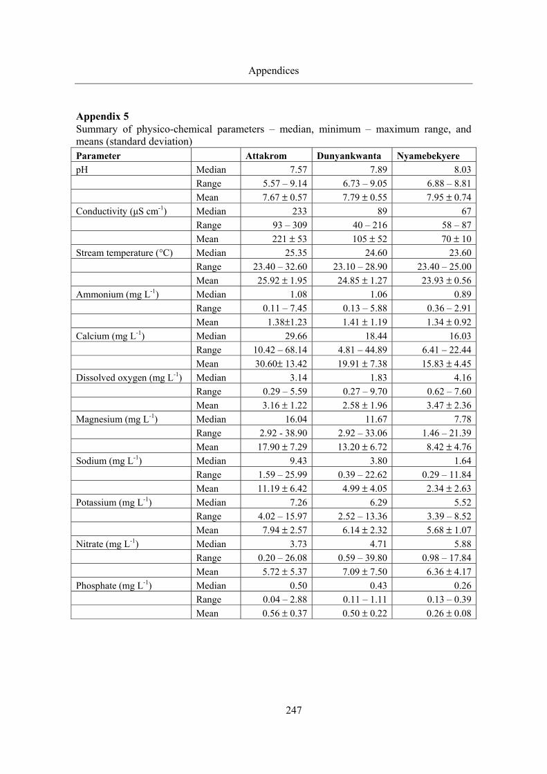
Appendices

247

Appendix 5 Summary of physico-chemical parameters – median, minimum – maximum range, and means (standard deviation) Parameter Attakrom Dunyankwanta Nyamebekyere pH Median 7.57 7.89 8.03 Range 5.57 – 9.14 6.73 – 9.05 6.88 – 8.81 Mean 7.67 ± 0.57 7.79 ± 0.55 7.95 ± 0.74Conductivity (µS cm-1) Median 233 89 67 Range 93 – 309 40 – 216 58 – 87 Mean 221 ± 53 105 ± 52 70 ± 10Stream temperature (°C) Median 25.35 24.60 23.60 Range 23.40 – 32.60 23.10 – 28.90 23.40 – 25.00 Mean 25.92 ± 1.95 24.85 ± 1.27 23.93 ± 0.56Ammonium (mg L-1) Median 1.08 1.06 0.89 Range 0.11 – 7.45 0.13 – 5.88 0.36 – 2.91 Mean 1.38±1.23 1.41 ± 1.19 1.34 ± 0.92Calcium (mg L-1) Median 29.66 18.44 16.03 Range 10.42 – 68.14 4.81 – 44.89 6.41 – 22.44 Mean 30.60± 13.42 19.91 ± 7.38 15.83 ± 4.45Dissolved oxygen (mg L-1) Median 3.14 1.83 4.16 Range 0.29 – 5.59 0.27 – 9.70 0.62 – 7.60 Mean 3.16 ± 1.22 2.58 ± 1.96 3.47 ± 2.36Magnesium (mg L-1) Median 16.04 11.67 7.78 Range 2.92 - 38.90 2.92 – 33.06 1.46 – 21.39 Mean 17.90 ± 7.29 13.20 ± 6.72 8.42 ± 4.76Sodium (mg L-1) Median 9.43 3.80 1.64 Range 1.59 – 25.99 0.39 – 22.62 0.29 – 11.84 Mean 11.19 ± 6.42 4.99 ± 4.05 2.34 ± 2.63Potassium (mg L-1) Median 7.26 6.29 5.52 Range 4.02 – 15.97 2.52 – 13.36 3.39 – 8.52 Mean 7.94 ± 2.57 6.14 ± 2.32 5.68 ± 1.07Nitrate (mg L-1) Median 3.73 4.71 5.88 Range 0.20 – 26.08 0.59 – 39.80 0.98 – 17.84 Mean 5.72 ± 5.37 7.09 ± 7.50 6.36 ± 4.17Phosphate (mg L-1) Median 0.50 0.43 0.26 Range 0.04 – 2.88 0.11 – 1.11 0.13 – 0.39 Mean 0.56 ± 0.37 0.50 ± 0.22 0.26 ± 0.08

Appendices

248

Appendix 6 Total monthly nutrient load (kg) for nutrients from each catchment for the study period (computed with the Beale equation)

Attakrom Ca K Mg Na NH4-N NO3-N PO4-P Oct-05 1015441.2 331663.1 547928.0 260493.9 42162.0 172934.7 31424.7 Nov-05 83186.3 22612.7 44490.0 30186.9 3848.7 5266.9 1700.6 May-06 423201.6 133179.6 318486.7 60572.0 30166.6 88123.5 24304.9 Jun-06 343820.7 126536.5 265221.2 123092.8 22996.5 95473.8 11561.7 Jul-06 312964.1 91550.5 245749.0 147717.5 20636.4 70693.7 6005.5 Aug-06 211666.0 53471.9 153282.9 141396.2 11562.5 33633.8 4807.9 Sep-06 299270.1 52250.5 154222.5 105104.5 7612.2 19684.7 4039.0 Oct-06 774392.0 217529.1 603399.2 290241.9 55575.3 235776.5 23234.4 Nov-06 71683.3 32452.6 125209.1 37886.3 750.9 29696.9 1829.5 Dunyankwanta Ca K Mg Na NH4-N NO3-N PO4-P Oct-05 819229.2 541806.4 760701.8 212938.4 73712.5 354872.1 39832.2 Nov-05 14514.6 6149.6 7975.9 2486.8 1013.2 2034.1 258.9 May-06 3045449.4 1019666.9 2127927.4 643357.6 100166.7 449420.1 67740.7 Jun-06 1351328.2 237251.9 655304.7 85403.1 56981.8 199232.6 27831.6 Jul-06 1301050.3 189717.3 490862.8 316508.0 130374.8 363331.6 24917.9 Aug-06 687821.0 173951.5 554550.2 326360.3 61418.7 131603.8 18718.7 Oct-06 3086887.9 776463.7 1552197.5 628667.2 225976.0 785068.3 37750.0 Nov-06 1324704.2 437292.9 1383350.5 424513.7 91666.5 729389.3 41802.2 Nyamebekyere Ca K Mg Na NH4-N NO3-N PO4-P Oct-05 454428.6 271273.9 330236.0 72176.9 34126.2 337166.9 9666.4 Jun-06 99585.4 22764.4 30201.1 6619.7 6390.9 79168.3 1441.3 Jul-06 1886813.7 295376.0 127158.0 25174.2 182461.7 432183.9 27337.8 Oct-06 406807.1 133622.5 199679.4 47354.9 30235.2 99871.7 8505.3

Appendices

249

Appendix 7 Intensive Stream Biosurvey Form Notes A. General Characteristics 1 Sampling point

description Distinctive color, appearance or smell of stream water

2 Width stream channel Estimation of the width of the streambed covered by water from bank to bank

3 Stream depth Average estimate of stream depth 4 Local Land Use Activities present within 1/4 mile up-stream of and

adjacent to the site 5 Established weir type Type of weir at sampling sites B. Habitat Assessment 1 Shelter The type of shelter (e.g., rocks, branches, debris) available

for fish, insects, and snails 2 Pool substrate Type of bottom substrate (e.g. mud, sand, gravel, or

mixed) 3 Pool variability Types of pools found in stream (e.g. large-shallow, large-

deep, small-shallow, and small-deep) which may be formed during periods of low flow

4 Sediment deposition Occurrence of deposited sediments in stream channel which creates changing stream bottom

5 Channel sinuosity The meandering of a stream, whether winding with variety of habitats or straight with unvarying velocity

6 Channel flow status Percent of the existing channel that is filled with water 7 Bank protection Presence of natural vegetation that covers the stream bank

reducing erosion. 8 Condition of banks Erosion potential and status of stream bank, i.e. slope of

bank, unvegetated banks, exposed tree roots 9 Riparian zone Width of natural vegetation from the edge of the stream

bank that is a buffer zone and controls erosion. Adapted from USEPA, 2005

Appendices

250

Appendix 8 Stream habitat survey summary Site Stream

description Channel width (m)

Stream depth (m)

200-m radius

Stream substrate

Shelter type

Pools Channel flow

Bank slope

Bank erosion

Attakrom Shallow flow 0.5-3.0 0.2-1.0 Maize farms, tall grasses

Sandy with small stones

Bank foliage, debris

Few and isolated

70% of channel to flooding

Little slope, flat

None

Dunyankwanta Reddish brown water after storms

1.5 0.4-1.2 Mixed crops, natural foliage

Sandy, with underlying clay

Bamboo plant roots, natural foliage

Only one observed

40% of channel to flooding

Sharp slope, >50º

None

Nyamebekyere Shallow flow 2 0.5 Forest trees, natural foliage

Sandy, small stones, clayey

Tree roots, leaf litter, natural foliage

Few and isolated

50% of channel to flooding

Flat None

Mankranso Turbid after storms, cloudy with silt or organic matter

5.0-3.0 1.0-3.0 Mainly tall grasses

Sand with gravels

Submerged grasses

Few large shallow

50% of channel to flooding

Slight slope

None

Kunsu Muddy, silted water after storms, brownish from decaying vegetation

5.0-15.0 0.5-1.5 Small trees, brush

Clay Hanging bank foliage

None 40 % - 80%

Sharp slope, >50º

None

Appendices

251

Site Stream description

Channel width (m)

Stream depth (m)

200-m radius

Stream substrate

Shelter type

Pools Channel flow

Bank slope

Bank erosion

Nyasiso Turbid after storms, cloudy with silt or organic matter

7.0 0.5-2.0 Few fields Natural foliage

Submerged and hanging bank foliage

Few large, many small

10% of channel to flooding

Little slope

None

Borosase Turbid after storms, cloudy with silt or organic matter

6.0 -100.0

0.5-7.0 Farm fields, secondary forests

Fine silt, muddy

Tree roots, hanging foliage, debris

None 20% - 80%

Sloping, >45º

Some

Afrensini Clear, fast flowing water

5.0 – 10.0

0.5-1.0 Small trees, brush

Stony, gravelly

Tree roots, hanging foliage

None 20% - 80%

Sloping, >40º

None

Akuapem Milky brown water, perennial

5.0 – 10.0

Small trees, brush

Muddy Tree roots, hanging foliage

None 20% of channel to flooding

Sloping, >40º

None

Ntabanu Natural milky brown color, perennial

15.0-45.0

0.5-6.0 Farms, secondary forests

Muddy Tree roots, hanging foliage

None 10% - 30%

Sloping >45º

Some

Beposo Water color varies throughout year, perennial

7.0-1000.0

1.0-8.0 Farms, trees, brush

Sandy with gravel, small stones

Tree roots and hanging foliage

None 1% of channel to flooding

Sloping <25º

Some

Appendices

252

Appendix 9 Sampled macroinvertebrate taxa, with number of individuals and percentage abundance per Family Family Order Total # % Abundance Macroinvertebrates Gyrinidae Coleoptera 2957 43.21Baetidae Ephemeroptera 2444 35.78Penaeidae Decapoda 427 6.25Chironomidae Diptera 404 5.92Veliidae Hemiptera 96 1.41Calopterygidae Odonata 89 1.30Planorbidae Pulmonata 73 1.07Caenidae Ephemeroptera 50 0.73Belostomatidae Hemiptera 49 0.72Gerridae Hemiptera 43 0.63Notonectidae Hemiptera 36 0.53Libellulidae Odonata 36 0.53Dytiscidae Coleoptera 28 0.41Psychodidae Diptera 24 0.35Ampullariidae Architaenioglossa 20 0.29Culicidae Diptera 14 0.20Oligochaeta Oligochaeta 11 0.16Lymnaeidae Pulmonata 9 0.13Planorbidae Basommatophora 8 0.12Thiaridae Mesogastropoda 4 0.06Nepidae Hemiptera 4 0.06Heptageniidae Ephemeroptera 3 0.04Gomphidae Odonata 2 0.03Hydropsychidae Trichoptera 2 0.03Syrphidae Diptera 1 0.01Hydrometridae Hemiptera 1 0.01Hirudinidae Arhynchobdellida 1 0.01Subtotal individuals 6836 82.06 Other taxa Cyprinidae Cypriniformes 1247 83.52Anura Anura 176 11.79Cichlidae Perciformes 68 4.55Claridae Siluriformes 2 0.13Subtotal individuals 1493 17.94 TOTAL 8329 100.00

Appendices

253

Appendix 10 Sampled macroinvertebrate taxa, with number of Family, number of individuals, and percentage composition per Order. Order # Families # Individuals % Composition

Macroinvertebrates

Coleoptera 2 2979 43.62

Ephemeroptera 3 2497 36.56

Diptera 4 443 6.49

Decapoda 1 427 6.25

Hemiptera 6 229 3.35

Odonata 3 127 1.86

Pulmonata 2 82 1.20

Architaenioglossa 1 20 0.29

Oligochaeta 1 11 0.16

Basommatophora 1 8 0.12

Mesogastropoda 1 4 0.06

Trichoptera 1 2 0.03

Arhynchobdellida 1 1 0.01

Subtotal 27 6830 100.00

Other orders

Cypriniformes 1 709 47.49

Unknown fish fry - 538 36.06

Anura 1 176 11.79

Perciformes 1 68 4.55

Siluriformes 1 2 0.13

Subtotal 4 1493 100.00

Appendices

254

Appendix 11 Total macroinvertebrate numbers sampled per site. A=Attakrom, B=Dunyankwanta, C=Nyamebekyere, D=Mankranso, E=Kunsu, F=Nyasi, G=Borosase, H=Afrensini, I=Akuapem, J=Ntabanu, K=Beposo.

Family Numbers A B C D E F G H I J K

Ampullariidae 20 5 0 0 5 8 2 0 0 0 0 0

Anura 176 2 1 0 8 58 33 50 0 23 0 1

Baetidae 2444 14 0 1 1537 449 191 17 121 29 21 64

Belostomatidae 49 0 0 0 37 4 0 2 0 3 0 3

Caenidae 50 4 0 0 40 2 1 0 0 0 0 3

Calopterygidae 89 0 0 9 24 36 6 2 6 3 1 2

Chironomidae 404 3 4 0 80 61 39 3 2 174 12 26

Cichlidae 68 0 0 0 1 1 4 0 0 1 8 53

Claridae 2 1 0 0 0 0 0 0 0 0 1 0

Culicidae 14 0 0 0 4 0 2 0 0 7 1 0

Cyprinidae 1247 16 0 0 456 31 13 8 0 174 261 288

Dytiscidae 28 0 0 0 3 2 2 0 0 21 0 0

Gerridae 43 2 0 0 28 4 2 0 0 5 1 1

Gomphidae 2 0 0 0 0 1 0 0 0 1 0 0

Gyrinidae 2951 12 16 0 110 7 13 1 6 111 558 2117

Heptageniidae 3 0 0 0 1 0 0 0 0 2 0 0

Hirudinidae 1 1 0 0 0 0 0 0 0 0 0 0

Hydrometridae 1 0 0 0 0 0 0 0 0 0 1 0

Hydropsychidae 2 0 1 0 0 0 1 0 0 0 0 0

Libellulidae 36 3 1 0 20 0 5 0 0 0 4 3

Lymnaeidae 9 0 0 0 1 0 0 0 0 0 0 8

Nepidae 4 0 0 0 0 0 1 0 0 1 1 1

Notonectidae 36 1 4 1 2 0 1 0 0 26 1 0

Oligochaeta 11 1 0 0 2 6 1 0 0 1 0 0

Penaeidae 427 0 2 0 109 40 9 5 2 194 9 57

Planorbidae 73 1 6 0 6 41 4 8 1 1 5 0

Planorbidae 8 0 0 0 7 0 1 0 0 0 0 0

Psychodidae 24 0 0 6 13 0 0 0 0 5 0 0

Syrphidae 1 0 0 0 0 1 0 0 0 0 0 0

Thiaridae 4 0 0 0 4 0 0 0 0 0 0 0

Veliidae 96 1 0 0 3 1 2 2 0 13 26 48

Appendices

255

Appendix 12 Total number of macroinvertebrate taxa (S), total number of individuals (N), Margalef’s index of richness (d), Pielou’s evenness index J), Shannon index (H′) and Simpson’s Diversity Index (1-λ). A=Attakrom, B=Dunyankwanta, C=Nyamebekyere, D=Mankranso, E=Kunsu, F=Nyasi, G=Borosase, H=Afrensini, I=Akuapem, J=Ntabanu, K=Beposo.

S N d J' H' 1-λ A0905 6 20 1.67 0.83 1.5 0.76A1005 4 9 1.37 0.88 1.21 0.75 A0606 2 4 0.72 0.81 0.56 0.5 A0806 7 23 1.91 0.76 1.48 0.74 A1006 6 11 2.09 0.93 1.67 0.87 B0905 5 28 1.2 0.74 1.2 0.63 B1006 4 7 1.54 0.83 1.15 0.71C0905 1 9 0 0 0 0 C1006 3 8 0.96 0.67 0.74 0.46 D0905 9 164 1.57 0.54 1.19 0.54 D1005 7 52 1.52 0.5 0.98 0.43 D1105 9 160 1.58 0.57 1.26 0.65 D1205 10 217 1.67 0.62 1.42 0.7 D0506 8 41 1.88 0.8 1.65 0.78 D0606 9 454 1.31 0.26 0.57 0.27 D0706 8 130 1.44 0.38 0.8 0.35 D0806 12 196 2.08 0.49 1.22 0.6 D0906 4 14 1.14 0.89 1.24 0.74 D1006 6 147 1 0.46 0.82 0.4 D1106 5 153 0.8 0.59 0.94 0.51 D1206 7 773 0.9 0.12 0.23 0.08 E0905 4 11 1.25 0.75 1.03 0.6 E1005 7 175 1.16 0.39 0.77 0.34 E1105 7 48 1.55 0.75 1.45 0.72 E1205 10 40 2.44 0.86 1.98 0.86 E0506 7 175 1.16 0.39 0.77 0.34 E0606 4 18 1.04 0.99 1.37 0.78 E0706 6 131 1.03 0.38 0.68 0.33 E0806 1 19 0 0 0 0 E0906 8 40 1.9 0.89 1.85 0.84 E1006 3 12 0.8 0.87 0.96 0.62 E1106 6 42 1.34 0.8 1.43 0.74 E1206 5 42 1.07 0.86 1.38 0.74F0905 5 6 2.23 0.97 1.56 0.93 F1005 5 12 1.61 0.77 1.23 0.67 F1205 10 33 2.57 0.79 1.81 0.8 F0606 7 182 1.15 0.32 0.61 0.26 F0706 6 18 1.73 0.77 1.38 0.73 F0806 5 12 1.61 0.77 1.23 0.67F0906 5 38 1.1 0.51 0.82 0.41 F1006 4 6 1.67 0.9 1.24 0.8

S N d J' H' 1-λ F1106 6 18 1.73 0.84 1.51 0.78F1206 3 8 0.96 0.89 0.97 0.68 G0606 9 49 2.06 0.86 1.89 0.84 G1006 5 49 1.03 0.54 0.86 0.44 H0905 3 124 0.41 0.15 0.16 0.06 H1006 3 9 0.91 0.77 0.85 0.56 H1206 3 5 1.24 0.86 0.95 0.7I0905 4 10 1.3 0.92 1.28 0.78 I1205 7 241 1.09 0.6 1.17 0.65 I0106 9 45 2.1 0.78 1.71 0.77 I0206 6 42 1.34 0.83 1.5 0.74 I0506 7 215 1.12 0.46 0.89 0.4 I0606 7 58 1.48 0.76 1.48 0.74 I0706 4 13 1.17 0.83 1.16 0.68 I0806 5 30 1.18 0.64 1.04 0.56 I1006 5 49 1.03 0.62 1 0.59 I1106 7 27 1.82 0.67 1.31 0.66 I1206 3 65 0.48 0.56 0.62 0.38 J1005 2 11 0.42 0.99 0.69 0.55 J0106 6 19 1.7 0.75 1.34 0.66 J0206 5 469 0.65 0.14 0.22 0.09 J0506 3 112 0.42 0.16 0.18 0.07 J0606 4 22 0.97 0.48 0.66 0.33 J0706 4 15 1.11 0.52 0.72 0.37 J0806 3 22 0.65 0.55 0.6 0.33 J1006 5 75 0.93 0.54 0.88 0.41 J1106 8 100 1.52 0.36 0.76 0.31 J1206 4 66 0.72 0.32 0.44 0.2 K1005 3 12 0.8 0.81 0.89 0.59 K1205 7 198 1.13 0.46 0.9 0.42 K0106 2 901 0.15 0.01 0.01 0 K0206 2 897 0.15 0.03 0.02 0.01 K0506 7 192 1.14 0.22 0.43 0.17K0606 5 31 1.16 0.58 0.93 0.5 K0706 6 36 1.4 0.77 1.38 0.68 K0806 4 21 0.99 0.87 1.21 0.71 K1006 4 62 0.73 0.9 1.25 0.71 K1106 10 50 2.3 0.69 1.58 0.68 K1206 6 275 0.89 0.51 0.91 0.47

Appendices

256

Appendix 13 Summary of stream physico-chemistry and nutrient ion concentrations. Median, range (minimum and maximum), and mean (standard deviation)

Parameter H2 M2 L1 M3 L3 HM4 Ofin1 Ofin2

pH Median 7.45 7.74 7.67 7.79 7.71 7.75 7.55 7.81

Range 6.74-8.43 6.45-8.64 6.44-8.68 6.90-8.23 7.03-8.22 6.77-8.65 6.61-7.97 6.49-8.14

Mean 7.49±0.44 7.68±0.51 7.63±0.54 7.72±0.37 7.65±0.41 7.71±0.53 7.51±0.39 7.69±0.43

Conductivity

(µS cm-1)

Median 92 88 74 78 88 105 117 115

Range 76-108 68-130 50-720 59-92 73-109 80-147 107-210 100-219

Mean 92±9.3 88±14.5 107±145 77±10.3 89±11.6 109±20.1 133±34.7 130±39.2

Temperature

(ºC)

Median 25.6 25.6 24.6 25.1 26.4 25.6 26.7 27.0

Range 22.4-27.4 21.8-28.1 20.0-25.8 19.9-27.6 21.1-27.1 21.5-27.1 23.0-28.0 23.5-28.4

Mean 25.5±1.08 25.5±1.49 24.4±1.45 24.8±1.96 25.7±1.79 25.1±1.51 26.3±1.45 26.7±1.30

Ammonium

(mg L-1)

Median 1.18 1.41 1.26 1.51 1.32 1.08 1.09 0.99

Range 0.30-6.72 0.23-5.02 0.25-4.52 0.66-4.25 0.28-8.87 0.53-5.05 0.33-5.31 0.19-5.46

Mean 1.98±1.80 1.91±1.48 1.77±1.34 1.95±1.28 2.18±2.25 1.70±1.32 1.67±1.37 1.62±1.60

Calcium

(mg L-1)

Median 14.43 15.23 13.23 16.83 15.23 16.83 17.64 16.83

Range 9.62-47.29 3.21-34.47 8.02-20.84 9.62-22.44 8.82-20.84 9.62-22.44 6.41-22.44 8.02-33.67

Mean 17.52±8.34 15.52±6.32 13.82±3.74 16.34±4.25 14.49±4.24 16.75±4.16 17.09±4.16 17.85±6.27

DO

(mg L-1)

Median 2.54 3.89 3.70 4.78 3.94 2.87 4.27 4.18

Range 0.08-3.88 1.67-5.37 1.95-7.74 0.76-5.54 1.89-7.80 0.11-3.99 0.01-8.70 0.09-8.30

Appendices

257

Parameter H2 M2 L1 M3 L3 HM4 Ofin1 Ofin2

Mean 2.34±1.09 3.65±1.05 3.81±1.24 4.17±1.48 3.85±1.73 2.51±1.43 4.04±2.04 4.28±1.83

Magnesium

(mg L-1)

Median 8.27 9.24 8.75 10.21 9.97 9.72 10.70 10.70

Range 0.49-19.45 1.94-26.45 2.82-15.56 6.81-17.50 5.35-17.50 1.09-16.53 3.89-15.56 3.89-13.61

Mean 8.80±4.42 9.91±5.28 9.10±3.34 10.96±3.58 11.39±3.93 9.37±3.84 10.52±2.75 10.31±2.76

Sodium

(mg L-1)

Median 9.24 9.05 8.04 9.24 8.42 11.07 16.36 14.44

Range 2.79-29.36 3.75-21.66 1.73-13.72 4.19-12.99 3.99-19.25 2.50-16.36 7.51-24.06 5.10-21.18

Mean 11.20±5.79 9.95±4.12 8.23±2.68 9.50±2.47 9.09±3.69 9.99±3.84 15.95±4.72 13.86±5.22

Potassium

(mg L-1)

Median 5.03 4.70 3.58 5.23 4.16 6.29 8.33 7.94

Range 3.39-28.56 2.71-9.29 1.94-5.66 3.39-17.18 2.81-7.84 4.16-12.10 5.13-15.68 6.39-15.00

Mean 7.56±6.77 4.94±1.47 3.69±0.94 6.52±4.13 4.51±1.51 6.74±2.18 9.34±2.85 8.83±2.70

Nitrate

(mg L-1)

Median 4.90 6.47 6.86 5.88 4.31 5.10 4.55 4.12

Range 1.18-30.59 1.57-48.63 1.18-30.39 1.96-26.08 0.01-24.12 1.18-26.27 1.37-32.94 1.96-28.63

Mean 8.80±7.85 11.26±11.12 11.26±9.61 11.00±8.95 8.32±7.85 8.76±7.61 9.23±9.31 9.87±9.34

Phosphate

(mg L-1)

Median 0.27 0.21 0.22 0.22 0.27 0.26 0.21 0.26

Range 0.12-2.07 0.11-0.52 0.13-0.45 0.07-0.35 0.13-0.52 0.21-1.01 0.07-1.09 0.07-0.87

Mean 0.38±0.36 0.23±0.10 0.25±0.09 0.22±0.08 0.29±0.10 0.35±0.20 0.29±0.24 0.30±0.18

ACKNOWLEDGEMENTS

A long journey begins with a first step and is consistently assisted by people whose timely contributions guide the process to its successful end. There are those who have taught, advised, encouraged, guided, opened doors, and even when not immediately apparent, have been instrumental in strengthening my will to achieve my full potential; this PhD is but one facet of an ongoing process. There are many who have contributed in their various ways, on both academic and personal fronts, and I would like to acknowledge my appreciation.

The genesis of my research began in early 1998 with discussions with Prof Chris Gordon of the University of Ghana, who pointed out the lack of basic knowledge on the impact of land based activities on the aquatic realm. In 1999, with the assistance of the Director of the Africa and Madagascar Programme of the World Wild Fund for Nature (WWF), Prof. Yaa Ntiamoa-Baidu, I was awarded a partial travel grant to undergo a three month attachment with the Royal Netherlands Institute of Marine Research - NIOZ, the Netherlands. At NIOZ, the support of Prof. Theunis Piersma and the additional financial support from the LOICZ programme (Land Ocean Interactions in the Coastal Zone) and START (SysTem for Analysis, Research, and Training), both units of the Earth Systems Science Partnership, resulted in the development of first version of the PhD research proposal. Although it would take me a several years (and two sons later) to eventually begin the PhD, this initial investment and collaboration significantly influenced my preparation for the PhD, for which I am sincerely grateful.

In due time, and in my estimation, in the most desirable of circumstances, I became one of the first PhD scholars of United Nations University – Institute of Environment and Human Security (UNU-EHS), in collaboration with ZEF. I am indebted to UNU and the GLOWA project for their financial support, and to those who were involved in the selection process - Prof. Bogardi (UNU-EHS), Prof. Asenso-Okyere (University of Ghana), and Prof. Vlek (ZEF). Prof. Vlek also played a significant role as my principal supervisor. I must also acknowledge the valuable inputs of my other supervisors, Prof. Schmidtlein from the Geography Department, University of Bonn; Prof. Gordon, whose mentoring and consistent encouragement for more than 15 years is deeply valued. I would also like to express my deep gratitude to Dr. Fabrice Renaud (UNU-EHS) for his unrelenting moral support and counsel throughout the entire thesis process. As my academic coach, he reliably provided the appropriate doses of encouragement and space required to maintain my sanity! I appreciate the assistance of Dr. Charles Rodgers, who found the time to guide me through the maze of hydrological calculations; Dr. Luna Bharati, who helped me refine the thesis focus; Dr. Guido Lechters for statistical advice, Mrs. Margaret Jend for her thorough editing, and Dr. Omar Ahmad of the School of Public Health, University of Ghana, not only for impromptu discussions in statistics and systemic thinking, but also for his invaluable friendship. I also want to thank my colleagues at UNU-EHS for their enthusiastic discussions and direction whenever I was ‘stuck’ – Alex, Andrea, Marcus, Maren and Marion.

I would like to express my gratitude to the administrative staff of the various departments I have been affiliated with for the duration of the study – GLOWA, UNU-EHS, and ZEF. I especially thank Mrs. Carlota Schneider for her warm assistance with both

personal and academic issues in Ghana and Germany; Mrs. Rosemary Zabel who has reliably rescued me many times from the complications of various formalities. To those at the Ghana GLOWA office who were extremely supportive in various aspects of the fieldwork set-up - Dr. Barry, Dr. Andreini, Raymond Kasei, Dr. Antwi – I appreciate all your efforts. My work would not have run as smoothly as it did without the extremely reliable field assistants, SK (Soil Research Institute, Kumasi) and Emmanuel (GLOWA) that I consider myself blessed to have found. Wofa, all this would not have been possible without your professional work but yet protective and brotherly care of me for the entire duration of my stay in Kumasi (and even afterwards). It was also a pleasure working with all the community members at the different sites who were involved with various aspects of the field work, especially the teachers at Attakrom, Dunyankwanta and Nyamebekyere. I would also like to express my thanks to Mr. Ankrah and Mr. Ansah of the Volta Basin Research Project, University of Ghana, for their assistance in macroinvertebrate identification and to all the laboratory staff at the Soil Research Institute, Kumasi, for the chemical analyses, especially Tony, Owusu, and Dr. Tetteh. To the Ghanaian researchers who were involved in the VINVAL project, I appreciate the candid interest in my work and assistance with fieldwork set up, data collection, as well as past reports. I especially thank Dr. Winston Andah and Dr. Fred Amu-Mensah for their personal involvement at all stages of the research. I would also like to thank all my colleagues at the Department of Oceanography & Fisheries, University of Ghana, for their support and encouragement to reach the finishing line. I look forward to returning and working with the team once again.

The duration of the research has also been marked with personal achievements and being able to manage parallel lives was made possible with the support and special friendships of those who enriched my life in their very unique ways – Rodrigue Noundou, Xiaomeng Shen and Boris Stähly, Evalyn Katabaro, Olivia Dunn, Francesca Burchi, Hong Ching Goh, Daniel Callo-Concha, Carme Costa, Dilys Kpongor, Kofi Nyarko, Patricia Aidam, Edward Nketiah-Amponsah, Emmanuel Obuobie, Benedicta Fosu-Mensah, Abdul Salam Lodhi, Maria Chambers, Norman Steinmeier.…, and my dear friends in Ghana – George Wiafe, Joshua Ndubuisi, and Jemima Jackson. To Uncle Ken, your assistance during this period, especially with the kids, is deeply appreciated.

To my family, you have been my pillar and my strength and to you I dedicate this thesis. To my mom, whose fierce love for her grandchildren enabled her to make significant and appreciated sacrifices despite her poor state of health; my dad whose calm strength has held us together all through the juggling moments; and my brother Raymond, whose support, love and sense of humor sustained me long before this process began. To the loves of my life, my boys, Levan and Jordan, who have suffered through frequent periods of my absence for most of their short lives, my work here is done and a new chapter finally begins!

In God there is Ultimate Glory…