�����������������

Citation: DeCastro, A.L.; Juliano,

T.W.; Kosovic, B.; Ebrahimian, H.;

Balch, J.K. A Computationally

Efficient Method for Updating Fuel

Inputs for Wildfire Behavior Models

Using Sentinel Imagery and Random

Forest Classification. Remote Sens.

2022, 14, 1447. https://doi.org/

10.3390/rs14061447

Academic Editors: Luis A. Ruiz and

Andrew T. Hudak

Received: 1 February 2022

Accepted: 15 March 2022

Published: 17 March 2022

Publisher’s Note: MDPI stays neutral

with regard to jurisdictional claims in

published maps and institutional affil-

iations.

Copyright: © 2022 by the authors.

Licensee MDPI, Basel, Switzerland.

This article is an open access article

distributed under the terms and

conditions of the Creative Commons

Attribution (CC BY) license (https://

creativecommons.org/licenses/by/

4.0/).

remote sensing

Communication

A Computationally Efficient Method for Updating Fuel Inputsfor Wildfire Behavior Models Using Sentinel Imagery andRandom Forest Classification

Amy L. DeCastro 1,2,* , Timothy W. Juliano 1 , Branko Kosovic 1 , Hamed Ebrahimian 3

and Jennifer K. Balch 2

1 National Center for Atmospheric Research, Boulder, CO 80307, USA; tjuliano@ucar.edu (T.W.J.);branko@ucar.edu (B.K.)

2 Department of Geography, University of Colorado Boulder, Boulder, CO 80309, USA;jennifer.balch@colorado.edu

3 Department of Civil and Environmental Engineering, University of Nevada Reno, Reno, NV 89557, USA;hebrahimian@unr.edu

* Correspondence: decastro@ucar.edu

Abstract: Disturbance events can happen at a temporal scale much faster than wildland fire fueldata updates. When used as input for wildland fire behavior models, outdated fuel datasets cancontribute to misleading forecasts, which have implications for operational firefighting, mitigation,and wildland fire research. Remote sensing and machine learning methods can provide a solutionfor on-demand fuel estimation. Here, we show a proof of concept using C-band synthetic apertureradar and multispectral imagery, land cover classes, and tree mortality surveys to train a randomforest classifier to estimate wildland fire fuel data in the East Troublesome Fire (Colorado) domain.The algorithm classified over 80% of the test dataset correctly, and the resulting wildland fire fueldata was used to simulate the East Troublesome Fire using the coupled atmosphere—wildland firebehavior model, WRF-Fire. The simulation using the modified fuel inputs, where 43% of originalfuels are replaced with fuels representing dead trees, improved the burn area forecast by 38%. Thisstudy demonstrates the need for up-to-date fuel maps available in real time to provide accurateprediction of wildland fire spread, and outlines the methodology based on high-resolution satelliteobservations and machine learning that can accomplish this task.

Keywords: wildland fire behavior model; fuel model; random forest; Sentinel; WRF-Fire

1. Introduction

The coniferous forests of the lower Rocky Mountains are innately disposed to wild-fire [1]. Trends toward a warmer, drier climate and rapid development of the wildland–urban interface (WUI) have increased wildfire risk to human life and property in thisregion [2]. Additionally, fuel accumulation through historic fire suppression and the rise infuel aridity have contributed to the risk of more severe wildfires [3]. Wildfire frequencyand severity are increasing in the Western United States [4], and the largest, most severefires have occurred since 2004 [5], motivating national discussions on risk mitigation [6].

Wildfire behavior models may be used effectively to forecast fire area, propagationdirection, and other metrics essential to operational firefighting, fuel treatment, and ouroverall understanding of wildfire [7]. Fuel characteristics including fuel load depth, percentmoisture of extinction, vegetation type, particle size, and heat content are important inputsfor these models. Quantifying fuel characteristics in an accurate and timely way has beenone of the main challenges of wildfire mitigation and operational management [8]. Thesemodels rely on accurate fuel data, and when data are available, the behavior models maybe used reliably in pre-wildfire mitigation, and in active-fire suppression and management.However, wildfire fuels are dynamic on multiple time scales, from their response to hourly

Remote Sens. 2022, 14, 1447. https://doi.org/10.3390/rs14061447 https://www.mdpi.com/journal/remotesensing

Remote Sens. 2022, 14, 1447 2 of 12

atmospheric conditions to their response to multi-year disturbance events, such as droughtor insect outbreaks. The publication of the fuel inputs commonly used for wildfire behaviormodeling may occur at a frequency outpaced by these disturbance events. However, thesedatasets provide a robust foundation that may be mindfully adjusted to provide wildfirebehavior models with updated fuel information.

LANDFIRE [9], a program that develops and publishes national geospatial datasets,hosts a suite of wildfire fuel datasets used by fire scientists and forest management teamsto suppress active wildfire and plan mitigation strategies. The LANDFIRE datasets includethe Scott and Burgan 40 fuel models [10], which are commonly used in wildfire behaviormodeling. The fuel models are profiles of fuel characteristics including fuel bed depth, fuelload, fuel moisture of extinction, vegetation composition, and surface-area-to-volume ratio.Most fuel data sets are created by mapping (or ‘crosswalking’ in fuel modeling terminology)remotely sensed data, such as satellite reflectance values and fuel characteristics used inwildfire behavior models. To determine the appropriate fuel model for each location in a30 m × 30 m grid across the contiguous United States (CONUS), the fuel data integrateremote sensing data, system ecology, gradient modeling, and landscape simulation. Com-posing fuel data sets is time consuming, and requires significant planning, resources, andfunding. Understandably, the data sets are infrequently updated, which can be problematicwhen used as input for wildfire behavior modeling, particularly when used for operationalwildfire management.

Here we present a method of refreshing fuel layer data using a case study of 2020East Troublesome Fire in Colorado. While the most current LANDFIRE data availableat the time of the fire showed the domain as healthy timber, shrub, and grassland, firerecords show that the East Troublesome Fire burned through significant amounts of deadand downed timber; while this case study requires adjusting the fuel data to reflect beetleinfestation and blowdown due to wind events, the same method could be applied to otherscenarios, such as representing fuels before recursive burning or a shift in vegetation type.The overall goals of this work are to estimate tree mortality severity using a random forest(RF) model trained on C-band synthetic aperture radar (C-SAR) Sentinel-1 data, raw bandsand vegetation indices from Sentinel-2 data, land cover vegetation classes from the UnitedStates Forest Service (USFS) Landscape Change Monitoring System (LCMS), and the Insectand Disease Detection Surveys (IDS) from the US Forest Service. We simulate a case studyof the East Troublesome Fire using both the generated fuel data and the LANDFIRE dataavailable at the time of the fire, and compare the simulations’ results with observed activefire data.

2. Materials and Methods2.1. The East Troublesome Fire Case Study

The East Troublesome Fire was detected on 14 October 2020 northeast of Kremmling,Colorado, in the Arapaho and Roosevelt National Forests. With low humidity recoveryovernight and high winds, the area was perfectly primed for fast wildfire conditions. Withinthe first 3 days, the fire spread to approximately 10,000 acres. Within 9 days, it had coverednearly 200,000 acres and crossed to the east side of the continental divide [11].

The East Troublesome Fire is an especially notable case study because it spread up-wards of 87,000 acres in a 24 h period (21–22 October 2020). At the time of the fire, theavailable LANDFIRE fuel data set reflected fuel conditions from 2016. In 2016, much ofthe fire’s domain was classified as standing healthy timber and shrub. However, between2016 and 2020, the timber in the fire domain experienced pine beetle outbreak, drought,and wind storms resulting in fuel conditions described as jackstraw—a tumble of very dry,downed, and standing trees [11]. Thus, we expect that a simulation of the East TroublesomeFire using the Scott and Burgan 40 fuel model layer available at the time of the fire wouldunderestimate the burned area, as much of the fire domain was represented as healthy,standing timber and shrub in the dataset.

Remote Sens. 2022, 14, 1447 3 of 12

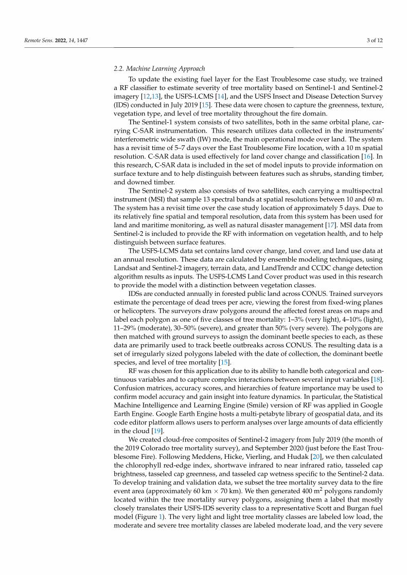
2.2. Machine Learning Approach

To update the existing fuel layer for the East Troublesome case study, we traineda RF classifier to estimate severity of tree mortality based on Sentinel-1 and Sentinel-2imagery [12,13], the USFS-LCMS [14], and the USFS Insect and Disease Detection Survey(IDS) conducted in July 2019 [15]. These data were chosen to capture the greenness, texture,vegetation type, and level of tree mortality throughout the fire domain.

The Sentinel-1 system consists of two satellites, both in the same orbital plane, car-rying C-SAR instrumentation. This research utilizes data collected in the instruments’interferometric wide swath (IW) mode, the main operational mode over land. The systemhas a revisit time of 5–7 days over the East Troublesome Fire location, with a 10 m spatialresolution. C-SAR data is used effectively for land cover change and classification [16]. Inthis research, C-SAR data is included in the set of model inputs to provide information onsurface texture and to help distinguish between features such as shrubs, standing timber,and downed timber.

The Sentinel-2 system also consists of two satellites, each carrying a multispectralinstrument (MSI) that sample 13 spectral bands at spatial resolutions between 10 and 60 m.The system has a revisit time over the case study location of approximately 5 days. Due toits relatively fine spatial and temporal resolution, data from this system has been used forland and maritime monitoring, as well as natural disaster management [17]. MSI data fromSentinel-2 is included to provide the RF with information on vegetation health, and to helpdistinguish between surface features.

The USFS-LCMS data set contains land cover change, land cover, and land use data atan annual resolution. These data are calculated by ensemble modeling techniques, usingLandsat and Sentinel-2 imagery, terrain data, and LandTrendr and CCDC change detectionalgorithm results as inputs. The USFS-LCMS Land Cover product was used in this researchto provide the model with a distinction between vegetation classes.

IDSs are conducted annually in forested public land across CONUS. Trained surveyorsestimate the percentage of dead trees per acre, viewing the forest from fixed-wing planesor helicopters. The surveyors draw polygons around the affected forest areas on maps andlabel each polygon as one of five classes of tree mortality: 1–3% (very light), 4–10% (light),11–29% (moderate), 30–50% (severe), and greater than 50% (very severe). The polygons arethen matched with ground surveys to assign the dominant beetle species to each, as thesedata are primarily used to track beetle outbreaks across CONUS. The resulting data is aset of irregularly sized polygons labeled with the date of collection, the dominant beetlespecies, and level of tree mortality [15].

RF was chosen for this application due to its ability to handle both categorical and con-tinuous variables and to capture complex interactions between several input variables [18].Confusion matrices, accuracy scores, and hierarchies of feature importance may be used toconfirm model accuracy and gain insight into feature dynamics. In particular, the StatisticalMachine Intelligence and Learning Engine (Smile) version of RF was applied in GoogleEarth Engine. Google Earth Engine hosts a multi-petabyte library of geospatial data, and itscode editor platform allows users to perform analyses over large amounts of data efficientlyin the cloud [19].

We created cloud-free composites of Sentinel-2 imagery from July 2019 (the month ofthe 2019 Colorado tree mortality survey), and September 2020 (just before the East Trou-blesome Fire). Following Meddens, Hicke, Vierling, and Hudak [20], we then calculatedthe chlorophyll red-edge index, shortwave infrared to near infrared ratio, tasseled capbrightness, tasseled cap greenness, and tasseled cap wetness specific to the Sentinel-2 data.To develop training and validation data, we subset the tree mortality survey data to the fireevent area (approximately 60 km × 70 km). We then generated 400 m2 polygons randomlylocated within the tree mortality survey polygons, assigning them a label that mostlyclosely translates their USFS-IDS severity class to a representative Scott and Burgan fuelmodel (Figure 1). The very light and light tree mortality classes are labeled low load, themoderate and severe tree mortality classes are labeled moderate load, and the very severe

Remote Sens. 2022, 14, 1447 4 of 12

tree mortality class is labeled high load. Each of the three resulting classes represents a fuelmodel in the slash–blowdown category of the Scott and Burgan fuel models, a categoryused to describe timber slash or downed fuel from wind damage, while ‘crosswalking’ fueldata to fuel models is a common practice [10,21], it should be noted that it is a subjectiveprocess [22]. Effort was made to best match the USFS tree mortality classes to the fuelmodels based on the guidance for choosing representative fuel models provided in theoriginal Scott and Burgan 40 fuel model publication [10]. To provide the RF model withdata that captures all possible surface features within the wildfire domain, 400 m2 polygonscapturing healthy vegetation, bare ground, urban areas, and water comprise an additionalclass of other. Altogether, the RF model is provided multispectral, C-SAR, and land coverclass input in sample spaces labeled either low load, moderate load, high load, or other.

Figure 1. Insect and Disease Detection Survey (IDS) tree mortality classes mapped to Scott andBurgan 40 fuel models from the slash-blowdown class. Polygons from the IDS were mapped to theirmost representative fuel models.

The full set of polygons was split randomly into 70% for training and 30% for testingby class. The image bands, calculated indices, and land cover classes were sampled withinthe polygons. The RF classifier was run for the composite July 2019 image and testedfor accuracy, before being applied to the September 2020 composite image. The modelconfiguration that optimized accuracy of classifying the test dataset included 100 decisiontrees, 5 variables per node split, a minimum leaf population of 1, an unlimited maximumnumber of leaf nodes, and a bag fraction of 0.5. Once classified, the fuel layer is written in.tif format such that it may be analyzed using Python and utilized as input for a wildfirebehavior model.

2.3. WRF-Fire

To examine the impact of the LANDFIRE fuel data on the evolution of the East Trou-blesome Fire, we used the weather research and forecasting (WRF) model [23] coupled to afire behavior model based on the coupled atmosphere–wildland fire environment [24,25].The coupled model is more commonly known as WRF-Fire [26]. In WRF-Fire, the meteo-rological grid is defined as in a typical WRF simulation; however, the fire grid is refinedto compute fine-scale changes in the fuel properties and track the evolution of the fireperimeter via a level-set method [27,28]. Using the Rothermel [29] parametrization, thewinds, fuel characteristics, and terrain slope on the fire grid determine the fire rate ofspread. Once a fire is ignited in the model, the burn rate of the fuel is determined viathe parametrization developed by Albini [30], which computes the amount of heat andmoisture released based on the fuel properties. The released energy then feeds back to theatmosphere, such that there is full coupling between the fire and atmosphere.

Remote Sens. 2022, 14, 1447 5 of 12

Our simulations are conducted using a two-domain setup, with the outer (d01) andinner (d02) domains covering an area of approximately 220,000 km2 and 32,000 km2,respectively, (Figure 2). By and large, our chosen model physics and dynamics optionsfollow the operational WRF-Fire modeling setup, called the Colorado Fire PredictionSystem, developed by the National Center for Atmospheric Research (NCAR). Optionsrelevant to this study include the following: (i) a horizontal grid cell spacing of 1000 mand 111.11 m, respectively, on the meteorological grid in d01 and d02; (ii) a horizontalgrid cell spacing of 27.77 m on the fire grid in d02 (subgrid ratio of 4 compared to themeteorological grid); (iii) 44 vertical grid cells in d01 and d02; and (iv) activating the Mellor–Yamada–Nakanishi–Niino (MYNN) [31] planetary boundary layer (PBL) parametrizationon d01, while d02 is run in large-eddy simulation (LES) mode. Furthermore, to determinethe impact of meteorology on the wildfire evolution and bolster our results related tofuel model sensitivity, we tested two different meteorological datasets used for initial andboundary condition forcing the North American Mesoscale Forecast System (NAM) andthe European Centre for Medium-Range Weather Forecasts Reanalysis v5 (ERA5).

Figure 2. The two-domain setup used in the WRF-Fire simulations. Terrain elevation is color-contoured according to the color bar (units in m) and state outlines are represented by the solid redlines.

During the preprocessing step for WRF-Fire, the fuel categories of the Scott and Burgan40 fuel class model are assigned to each fire grid cell. For the purposes of this study, wegenerate two different input files: one that contains the default Scott and Burgan 40 fuelclass model and one that contains the modified Scott and Burgan 40 fuel class modelfollowing our RF results, as described above. We refer to the former simulation as Controland the latter simulation as ML (abbreviation for modified layer). The original and modifiedScott and Burgan fuel model layers used in our WRF-Fire simulations are shown in Figure 3.We also utilize the 3-arc second Shuttle Radar Topography Mission (SRTM) terrain datafor the fuel grid. Recent developments by NCAR allow us to apply heterogeneous fuelmoisture content (FMC) values to our fire domain [32]. As an additional sensitivity test,we evaluate the impact of FMC by also conducting a simulation with constant FMC setto 9%, which is approximately equal to the domain-averaged value computed from theheterogeneous FMC data set (not shown).

In summary, we conducted a total of five simulations based on the various modelsensitivities discussed above: (1) NAM Control, (2) NAM ML, (3) NAM ML + ConstantFMC, (4) ERA5 Control, and (5) ERA5 ML. Each of our simulations began at 21 October

Remote Sens. 2022, 14, 1447 6 of 12

2020, 1800 UTC and ended at 22 October 2020, 1500 UTC. The fire is ignited from anactive perimeter (provided by the National Inter-agency Fire Center and shown in Figure 3)measured at 22 October 2020, 0020 UTC (6 h and 20 min after the simulation start timeto ensure sufficient spin-up time). We now show results from the various WRF-Firesimulations to highlight the relative impact of varying the fuel categories, meteorologicalforcing data set, and FMC.

Figure 3. The original (left) and modified (right) Scott and Burgan fuel model layers used in theWRF-Fire simulations. The active fire perimeter used to initiate the simulations is shown in white.Fuel categories represent the fuel type of the fuel model; slash–blowdown (SB), timber litter (TL),timber–understory (TU), shrub (SH), grass–shrub (GS), grass (GR), and nonburnable (NB).

3. Results

The RF algorithm correctly classified over 84% of the test data in the fire domain,and performed well at separating the tree mortality classes from the other class. The RFmisclassified 6.1% of the low load, <1% of the moderate load, and 8.7% of the high loadclasses as other. The confusion matrix for the classifier’s performance on the test dataset isgiven in Table 1. Table 2 shows the precision (positive predictive value), recall (true positiverate), and F1 score (weighted average of precision and recall) for each class.

Table 1. Confusion matrix for the classifier’s performance on the test dataset.

Other Low Load Moderate Load High Load

other 8505 337 257 52low load 31 256 120 105

moderate load 8 232 457 196high load 38 148 179 72

Table 2. Precision, recall, and F1-scores for the classifier’s performance on the test dataset.

Precision Recall F1-Score

other 0.927 0.992 0.958low load 0.520 0.252 0.340

moderate load 0.489 0.471 0.480high load 0.162 0.157 0.160

The fuel updating process resulted in changing a significant amount of the timber litterand timber–understory fuel classes in the original fuel model layer to slash–blowdownfuel classes in the modified fuel layer. Timber litter and timber–understory are fuel modelclasses in which the main fire carriers are litter such as pine needles or hardwood leavesshed from timber, and grasses, shrubs, litter, and moss, respectively. These are classestypically designated to healthy timber systems with finer fuels under the tree canopy. In

Remote Sens. 2022, 14, 1447 7 of 12

the semi-arid climate of the East Troublesome Fire case study, the wildfire rate of spreadgenerated from these fuel models is low to moderate. In contrast, the wildfire rate of spreadresulting from the slash–blowdown fuel models is moderate to high.

The WRF-Fire results from all sensitivity simulations are shown for two observedtimes in Figures 4 and 5, with time series of various burn area and burn rate statistics givenin Figure 6. Table 3 summarizes the forecast and observed areas for each of the simulations.

Figure 4. The sensitivity simulation results (solid yellow) using NAM meteorological data with theoriginal fuel inputs, the modified fuel inputs, and the modified fuel inputs with a constant 8% fuelmoisture content (labeled NAM Control, NAM ML, and NAM ML + Constant FMC, respectively),and the simulations using ERA5 with the original fuel inputs and the modified fuel inputs (labeledERA5 Control and ERA5 ML, respectively). The observed fire perimeter (solid magenta line) wascaptured aerially at 06:40 UTC on 22 October 2020 .

Figure 5. As in Figure 4, but for 02:40 UTC on 23 October 2020.

Overall, WRF-Fire underpredicts the East Troublesome Fire burn area regardless ofthe model setup explored in this study. Nonetheless, we find that modifying the fuel layerhas the largest positive impact compared to modifying meteorological forcing data setor the FMC. Conducting simulations using the default Scott and Burgan fuel model (thefuel data that was available to incident commanders at the start time of the fire) resultsin a much more substantial underprediction of the burned area compared with using theupdated fuel layer. As a result, the burned area prediction better matches the observedburned area, shown visually in Figures 4 and 5 and quantitatively in Figure 6 and Table 2.Additionally, our results show that forcing WRF-Fire with NAM leads to better agreement

Remote Sens. 2022, 14, 1447 8 of 12

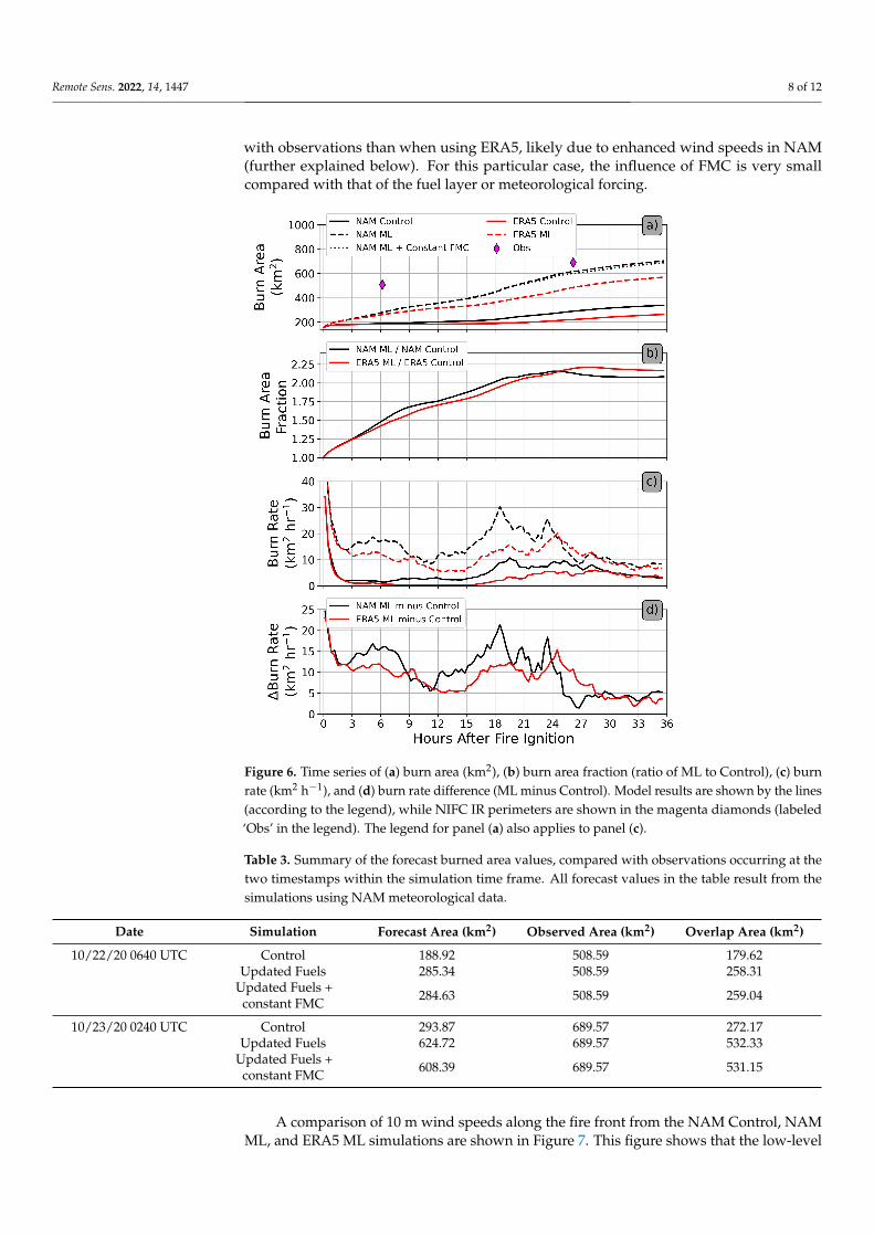
with observations than when using ERA5, likely due to enhanced wind speeds in NAM(further explained below). For this particular case, the influence of FMC is very smallcompared with that of the fuel layer or meteorological forcing.

Figure 6. Time series of (a) burn area (km2), (b) burn area fraction (ratio of ML to Control), (c) burnrate (km2 h−1), and (d) burn rate difference (ML minus Control). Model results are shown by the lines(according to the legend), while NIFC IR perimeters are shown in the magenta diamonds (labeled‘Obs’ in the legend). The legend for panel (a) also applies to panel (c).

Table 3. Summary of the forecast burned area values, compared with observations occurring at thetwo timestamps within the simulation time frame. All forecast values in the table result from thesimulations using NAM meteorological data.

Date Simulation Forecast Area (km2) Observed Area (km2) Overlap Area (km2)

10/22/20 0640 UTC Control 188.92 508.59 179.62Updated Fuels 285.34 508.59 258.31

Updated Fuels +constant FMC 284.63 508.59 259.04

10/23/20 0240 UTC Control 293.87 689.57 272.17Updated Fuels 624.72 689.57 532.33

Updated Fuels +constant FMC 608.39 689.57 531.15

A comparison of 10 m wind speeds along the fire front from the NAM Control, NAMML, and ERA5 ML simulations are shown in Figure 7. This figure shows that the low-level

Remote Sens. 2022, 14, 1447 9 of 12

wind speeds are stronger in NAM ML compared with ERA5 ML supporting the notion thatthe WRF-Fire simulations with NAM initial and boundary condition forcing produce fasterfire spread largely due to enhanced low-level wind speeds. In fact, the largest differencesin the NAM ML and ERA5 ML lines correspond well with the largest difference in burnrate between NAM ML and ERA5 ML (Figure 6c). Furthermore, we find that the 10 mfire front wind speeds are quite similar between NAM Control and NAM ML. This resultsuggest that the large differences in the burned area forecasts between the Control andML simulations may be confidently attributed to the differences between the original andmodified fuel model layers and the resultant differences in fuel properties.

Figure 7. Time series of fire-front-averaged 10 m wind speed at model grid cells with active burning.We average across all horizontal grid cells where the fire rate of spread is >0.05 m s−1. Results fromthree select simulations are shown according to the legend.

4. Discussion

Examining the confusion matrix of the RF classifier output shows that the modelcorrectly classifies approximately 92.7% of the other category correctly, most frequentlymistaking it for the low class (4.2% of the time) in the test data set. A proportion of 52% ofthe low class was correctly classified, and was misclassified as the moderate class 21% ofthe time. The RF correctly classified 48.9% of the moderate class, mistaking it for the lowclass 28.8% of the time. Finally, the high class was correctly classified 16.2% of the time,while mistaken for the moderate class 41.2% of the time. This analysis shows that while themodel performs well at distinguishing between the other class and the slash–blowdownclasses, it has not been provided enough information to excel at classifying the differentseverity levels. This is likely due in part to uncertainty in the training data, particularlyin the tree mortality surveys as the aerial collection practices are subjective in nature [33].Similar issues may arise in applying this method to other scenarios, which highlights theimportance of including ancillary data when available and understanding the limitationsof any included datasets.

The data used to train the RF classifier and to classify images were chosen with theintent of capturing information on tree mortality throughout the fire domain. In the contextof a different set of known conditions, it would be necessary to choose data representativeof those conditions. Regardless, the operator would need an understanding of availabledata and how it translates to on-the-ground conditions. Providing the RF classifier withadditional information about the particular conditions just before a fire will likely improveclassification accuracy when implemented mindfully.

The development and implementation of the RF in this study was performed inGoogle Earth Engine, which gives the Gini impurity decreases of each random forestnode as a metric of feature importance. Examining the hierarchy of these values for theRF features shows that the chlorophyll red-edge index suggested by Meddens, Hicke,Vierling, and Hudak [20] is the most important feature (Figure 8). This index is particularlysensitive to chlorophyll, carotenoids, and anthocyanin production [34], which indicatevegetation senescence. There is an inevitable change in senescence simply due to the

Remote Sens. 2022, 14, 1447 10 of 12

seasonal changes between July 2019 (the time of the tree mortality surveys) and September2020 (the time just before the East Troublesome Fire). As the chlorophyll red-edge index isimportant to classification, senescence may be confounded with the intended classificationof tree mortality in this case. However, the C-SAR bands, which contribute informationon the surface texture and were intended to help distinguish between vegetation typesand standing and downed timber, were also highly important to the classification. Giventhe high degree of classification accuracy, this indicates that collectively the input dataprovided was adequate to train the RF, and that any cells classified as tree mortality due tothe signature of senescence are of minimal consequence.

Figure 8. The sum of the Gini impurity decreases across all node splits for each individual randomforest feature. The bars represent the importance of each feature, measured through the sum of allthe Gini impurity index decreases for each feature included in the random forest classifier.

Google Earth Engine runs in the cloud and houses several relevant remote sensingdata sets. Based on the methodology described in this study, it would be possible to developan operational system that provides fuel updates in real time on an on-demand basis, andwhich would be available to fire behavior analysts and incident commanders. We wouldadvise becoming familiar with the available data sets that are most relevant to the regionbeing simulated. Moving forward more remote sensing data will become available, andmay be used fruitfully for this purpose. Two additional Sentinel-1 satellites, both equippedwith C-SAR instrumentation, are scheduled for launch in 2022 and 2023, and are expectedto shorten the current revisit time for the system. One additional Sentinel-2 satellite isscheduled for launch in 2024, and will likewise shorten the revisit time and contributemultispectral imagery to the already established Sentinel-2 system. The fuel model datacurrently available provides a solid foundation for mindfully adjusting fuel layers priorto running simulations using wildfire behavior models. The incoming wealth of remotesensing data and modeling tools will only provide more opportunity for refreshing thisdata as needed.

5. Conclusions

This work presents an effective workflow for updating fuel data used in wildland firebehavior modeling. It builds on available fuel data and provides a solution to quantifyingfuel characteristics in an accurate and timely manner; while the East Troublesome casestudy focuses on dead, downed timber due to beetle infestation and wind events, theworkflow presented here may be applied to several types of disturbance events that affectwildland fire fuels, given the availability of relevant data. These methods were intentionallydeveloped using freely available data on the analysis and modeling platform, Google EarthEngine, to make them accessible to a broad user base, including wildland fire researchersand incident commanders. We anticipate that with the increase in wildland fire activity,

Remote Sens. 2022, 14, 1447 11 of 12

research, and response, as well as the increase in availability of remotely sensed data, thatthese methods will aid in improving wildland fire forecasts.

Author Contributions: Conceptualization, A.L.D. and T.W.J.; methodology, A.L.D. and T.W.J.; soft-ware, A.L.D. and T.W.J.; validation, A.L.D., B.K. and T.W.J.; formal analysis, T.W.J.; investigation,A.L.D.; resources, B.K.; data curation, A.L.D.; writing—original draft preparation, A.L.D. and T.W.J.;writing—review and editing, B.K., H.E., and J.K.B.; visualization, A.L.D. and T.W.J.; supervision, B.K.,H.E. and J.K.B.; project administration, B.K., H.E. and J.K.B.; funding acquisition, B.K. and H.E. Allauthors have read and agreed to the published version of the manuscript.

Funding: This work is supported through the National Science Foundation’s Leading Engineeringfor America’s Prosperity, Health, and Infrastructure (LEAP HI) program by grant number CMMI-1953333. We would also like to acknowledge high-performance computing support from Cheyenne(doi:10.5065/D6RX99HX) provided by NCAR’s Computational and Information Systems Laboratory,sponsored by the National Science Foundation.

Data Availability Statement: A Google Earth Engine script, which includes data acquisition, isavailable through the GitHub page: https://github.com/amydecastro/wildfire_fuel_update_in_GEE,accessed on 1 February 2022.

Acknowledgments: Michael J. Koontz provided valuable Google Earth Engine support as well asmanuscript feedback.

Conflicts of Interest: The authors declare no conflict of interest. The funders had no role in the designof the study; in the collection, analyses, or interpretation of data; in the writing of the manuscript, orin the decision to publish the results.

References1. Jain, T.B.; Nelson, A.S.; Bright, B.C.; Byrne, J.C.; Hudak, A.T. Biophysical Settings that Influenced Plantation Survival during the

2015 Wildfires in Northern Rocky Mountain Moist Mixed-Conifer Forests. J. For. 2022, 120, 22–36. [CrossRef]2. Radeloff, V.C.; Helmers, D.P.; Kramer, H.A.; Mockrin, M.H.; Alexandre, P.M.; Bar-Massada, A.; Stewart, S.I. Rapid growth of the

US wildland-urban interface raises wildfire risk. Proc. Natl. Acad. Sci. USA 2018, 115, 3314–3319. [CrossRef] [PubMed]3. Burke, M.; Driscoll, A.; Heft-Neal, S.; Xue, J.; Burney, J.; Wara, M. The changing risk and burden of wildfire in the United States.

Proc. Natl. Acad. Sci. USA 2021, 118, 2. [CrossRef] [PubMed]4. Parks, S.A.; Abatzoglou, J.T. Warmer and drier fire seasons contribute to increases in area burned at high severity in western US

forests from 1985 to 2017. Geophys. Res. Lett. 2020, 47, e2020GL089858. [CrossRef]5. Environmental Protection Agency, Climate Change Indicators: Wildfire. Available online: https://www.epa.gov/climate-

indicators/climate-change-indicators-wildfires (accessed on 26 January 2022).6. U.S. Department of Agriculture, Biden-Harris Administration Announces Over $1 Billion in Disaster Relief Funds for Post-

Wildfire and Hurricane Recovery. Available online: https://www.usda.gov/media/press-releases/2022/01/21/biden-harris-administration-announces-over-1-billion-disaster (accessed on 21 January 2022).

7. Cardil, A.; Rodrigues, M.; Ramirez, J.; de-Miguel, S.; Silva, C.A.; Mariani, M.; Ascoli, D. Coupled effects of climate teleconnectionson drought, Santa Ana winds and wildfires in southern Cali-fornia. Sci. Total Environ. 2001, 765, 142788. [CrossRef] [PubMed]

8. Keane, R.E.; Burgan, R.; van Wagtendonk, J. Mapping wildland fuels for fire man-agement across multiple scales: Integratingremote sensing, GIS, and biophysical modeling. Int. J. Wildland Fire 2001, 10, 301–319. [CrossRef]

9. Rollins, M.G. LANDFIRE: A nationally consistent vegetation, wildland fire, and fuel as-sessment. Int. J. Wildland Fire 2009, 18,235–249. [CrossRef]

10. Scott, J.H. Standard Fire Behavior Fuel Models: A Comprehensive Set for Use with Rothermel’s Surface Fire Spread Model; US Departmentof Agriculture, Forest Service, Rocky Mountain Research Station: Fort Collins, CO, USA, 2005.

11. Inciweb, East Troublesome Fire Information. Available online: https://inciweb.nwcg.gov/incident/7242/ (accessed on 1 June2021).

12. Earth Engine Data Catalog, Sentinel-1. Available online: https://developers.google.com/earth-engine/datasets/catalog/COPERNICUS_S1_GRD?hl=en (accessed on 1 June 2021).

13. Earth Engine Data Catalog, Sentinel-2. Available online: https://developers.google.com/earth-engine/datasets/catalog/COPERNICUS_S2_SR (accessed on 1 June 2021).

14. Earth Engine Data Catalog, USFS Landscape Change Monitoring System v2020.5. Available online: https://developers.google.com/earth-engine/datasets/catalog/USFS_GTAC_LCMS_v2020-5?hl=en (accessed on 1 June 2021).

15. U.S. Department of Agriculture, Forest Health. Available online: https://www.fs.fed.us/foresthealth/applied-sciences/mapping-reporting/detection-surveys.shtml (accessed on 10 June 2021).

Remote Sens. 2022, 14, 1447 12 of 12

16. Sentinel Online, Sentinel-1. Available online: https://sentinels.copernicus.eu/web/sentinel/user-guides/sentinel-1-sar/applications/land-monitoring (accessed on 13 January 2022).

17. Sentinel Online, Sentinel-2. Available online: https://sentinels.copernicus.eu/web/sentinel/user-guides/sentinel-2-msi/applications (accessed on 13 January 2022).

18. Breiman, L. Random forests. Mach. Learn. 2001, 45, 5–32. [CrossRef]19. Gorelick, N.; Hancher, M.; Dixon, M.; Ilyushchenko, S.; Thau, D.; Moore, R. Google Earth Engine: Planetary-scale geospatial

analysis for everyone. Remote Sens. Environ. 2017, 202, 18–27. [CrossRef]20. Meddens, A.J.; Hicke, J.A.; Vierling, L.A.; Hudak, A.T. Evaluating methods to detect bark beetle-caused tree mortality using

single-date and multi-date Landsat imagery. Remote Sens. Environ. 2013, 132, 49–58. [CrossRef]21. Anderson, H.E. Aids to Determining Fuel Models for Estimating Fire Behavior [Grass, Shrub, Timber, and Slash, Photographic Examples,

Danger Ratings]; USDA Forest Service General Technical Report; INT-Intermountain Forest and Range Experiment Station (USA):Ogden, UT, USA, 1982.

22. Krasnow, K.; Schoennagel, T.; Veblen, T.T. Forest fuel mapping and evaluation of LANDFIRE fuel maps in Boulder County,Colorado, USA. For. Ecol. Manag. 2009, 257, 1603–1612. [CrossRef]

23. Skamarock, W.C.; Klemp, J.B.; Dudhia, J.; Gill, D.O.; Barker, D.M.; Wang, W.; Powers, J.G. A Description of the Advanced ResearchWRF Version 2; National Center For Atmospheric Research Boulder Co Mesoscale and Microscale Meteorology Div.: Boulder, CO,USA, 2005.

24. Clark, T.L.; Coen, J.; Latham, D. Description of a coupled atmosphere–fire model. J. Wildland Fire 2004, 13, 49–63. [CrossRef]25. Coen, J.L. Modeling Wildland Fires: A Description of the Coupled Atmosphere-Wildland Fire Environment Model (CAWFE); National

Center for Atmospheric Research: Boulder, CO, USA, 2013; Volume 38.26. Coen, J.L.; Cameron, M.; Michalakes, J.; Patton, E.G.; Riggan, P.J.; Yedinak, K.M. WRF-Fire: Coupled weather–wildland fire

modeling with the weather research and forecasting model. J. Appl. Meteorol. Climatol. 2013, 52, 16–38. [CrossRef]27. Mandel, J.; Beezley, J.D.; Kochanski, A.K. Coupled atmosphere-wildland fire mod-eling with WRF 3.3 and SFIRE 2011. Geosci.

Model. Dev. 2011, 4, 591–610. [CrossRef]28. Muñoz-Esparza, D.; Kosovic, B.; Jiménez, P.A.; Coen, J.L. An accurate fire-spread algo-rithm in the Weather Research and

Forecasting model using the level-set method. J. Adv. Model. Earth Syst. 2018, 10, 908–926. [CrossRef]29. Rothermel, R.C. A Mathematical Model for Predicting Fire Spread in Wildland Fuels; Intermountain Forest Range Experiment Station,

Forest Service, US Department of Agriculture: Ogden, UT, USA, 1972; Volume 115, pp. 5–32.30. Albini, F.A.; Brown, J.K.; Reinhardt, E.D.; Ottmar, R.D. Calibration of a large fuel burn-out model. Int. J. Wildland Fire 1995, 5,

173–192. [CrossRef]31. Nakanishi, M.; Niino, H. An improved Mellor–Yamada level-3 model with con-densation physics: Its design and verification.

Bound.-Layer Meteorol. 2004, 112, 1–31. [CrossRef]32. McCandless, T.C.; Kosovic, B.; Petzke, W. Enhancing wildfire spread model-ling by building a gridded fuel moisture content

product with machine learning. Mach. Learn. Sci. Technol. 2020, 1, 305010. [CrossRef]33. Coleman, T.W.; Graves, A.D.; Heath, Z.; Flowers, R.W.; Hanavan, R.P.; Cluck, D.R.; Ryerson, D. Accuracy of aerial detection

surveys for mapping insect and disease disturbances in the United States. For. Ecol. Manag. 2018, 430, 321–336. [CrossRef]34. Gitelson, A.A.; Keydan, G.P.; Merzlyak, M.N. Three-band model for noninvasive estimation of chlorophyll, carotenoids, and

anthocyanin contents in higher plant leaves. Geophys. Res. Lett. 2006, 33. [CrossRef]