1

Computationally efficient and robust BIC-based

speaker segmentation

Margarita Kotti, Emmanouil Benetos, and Constantine Kotropoulos∗, Senior Member, IEEE

Dept. of Informatics, Aristotle University of Thessaloniki, Box 451, Thessaloniki 54124,

Greece, Tel: +30-2310-996361, Fax: +30-2310-998453

mkotti,empeneto,costas@aiia.csd.auth.gr

Abstract

An algorithm for automatic speaker segmentation based on the Bayesian Information Criterion (BIC)

is presented. BIC tests are not performed for every window shift (e.g. every milliseconds), as previously,

but when a speaker change is most probable to occur. This is done by estimating the next probable

change point thanks to a model of utterance durations. It is found that the inverse Gaussian fits best the

distribution of utterance durations. As a result, less BIC tests are needed, making the proposed system

less computationally demanding in time and memory, and considerably more efficient with respect to

missed speaker change points. A feature selection algorithm based on branch and bound search strategy

is applied in order to identify the most efficient features for speaker segmentation. Furthermore, a new

theoretical formulation of BIC is derived by applying centering and simultaneous diagonalization. This

formulation is considerably more computationally efficient than the standard BIC, when the covariance

matrices are estimated by other estimators than the usual maximum likelihood ones. Two commonly used

pairs of figures of merit are employed and their relationshipis established. Computational efficiency is

achieved through the speaker utterance modeling, whereas robustness is achieved by feature selection

and application of BIC tests at appropriately selected timeinstants. Experimental results indicate that the

proposed modifications yield a superior performance compared to existing approaches.

Index Terms

* Corresponding author

March 22, 2008 DRAFT

2

Automatic speaker segmentation, Bayesian Information Criterion, Speaker utterance duration distri-

bution, Inverse Gaussian distribution, Simultaneous diagonalization, Speech analysis.

I. I NTRODUCTION

Nowadays, a vast rise in multimedia archives has occurred, partially due to the increasing number of

broadcast programs, the decreasing cost of mass storage devices, the advances in compression techniques,

and the wide prevalence of personal computers. The functionality of such archives would be in doubt,

unless data management is employed. Data management is necessary for organizing, navigating, and

browsing the multimedia content, as is manifested by the MPEG-7 standard. Here, we focus on speech.

Speaker segmentation is an efficient tool for multimedia archive management. It aims to find the speaker

change points in an audio recording. Speaker segmentation finds numerous applications, since it is

a prerequisite for audio indexing, speaker identification/verification/tracking, automatic transcription,

and dialogue detection in movies. MPEG-7 audio low-level descriptors (e.g. AudioSpectrumProjection,

AudioSpectrumEnvelope) can be used to describe efficiently a speech recording [1]. In addition, MPEG-

7 high-level tools, (e.g. SpokenContent) exploit speakers’word usage or prosodic features that are also

useful for speaker segmentation. A large number of groups and research centers compete for improved

speaker segmentation. An example is the segmentation task administrated by theNational Institute of

Standards and Technology(NIST) [2]. NIST has also been working towards rich transcription evaluation

(NIST/RT). Rich transcription includes speaker segmentationas a part of its diarization task [3].

A. Related Work

Extensive work in speaker segmentation has been carried out for more than two decades. Three major

categories of speaker segmentation algorithms can be found: model-based, metric-based, andhybrid ones.

In model-based segmentation, a set of models is trained for different speaker classes andthe incoming

speech recording is classified using the trained models. Various methods have been used in order to create

generic models. Starting from the less complex case, a universal background model (UBM) is utilized to

separate speech from non-speech [4]. The UBM is trained by using a large volume of speech data off-line.

The algorithm can be used in real-time, because the models have been pre-calculated. Second, instead

of using just one generic model, two universal gender models(UGM), that discriminate between male

and female speakers can be used [5]. Third, the so-called sample speaker model (SSM) can be adopted

March 22, 2008 DRAFT

3

[5]. This is a predetermined, generic, speaker-independentmodel, which is progressively adapted into a

specific speaker-dependent one. Alternatively, an anchor model can be utilized, where a speaker utterance

is projected onto a subspace of reference speakers [6]. Finally, more sophisticated models can be created

with the help of hidden Markov models (HMMs) [7], [8], [9] or support vector machines (SVMs) [10].

Metric-based techniquesdetect the local extrema of a proper distance between neighboring windows

in order to segment an input recording. Various distances have been employed. For example, a weighted

squared Euclidean distance has been used, where the weights are updated by Fisher linear discriminant

analysis [11]. Another criterion is the generalized likelihood ratio (GLR) test [5], [6], [9], [12], [23].

The Kullback-Leibler divergence is also commonly employed. It is used either in conjunction with

the Bayesian Information Criterion (BIC) [12], [13] or independently [14]. Alternatively, second-order

statistics could be used [12]. Another closely related measure is the HotellingT 2 statistic, which is

combined with BIC to achieve a higher accuracy than the standard BIC for turns of short duration [15],

[16]. However, the most popular criterion is BIC [7], [12], [15], [17], [18], [19], [20], [21]. Commonly

used features in speaker segmentation are the mel-cepstrumcoefficients (MFCCs), applied in conjunction

with BIC [1], [4], [5], [7], [8], [9], [11], [12], [13], [15], [18], [20], [22]. A milestone variant of BIC-

based algorithms is DISTBIC, that utilizes distance-based pre-segmentation before applying BIC [12].

Most recently, BIC is compared to agglomerative clustering, minimum description length-based Gaussian

modeling, and exhaustive search. It is found that applying audio classification into speech, noise, and

music prior to speaker segmentation improves speaker segmentation accuracy [22]. An approach to

segmentation and identification of mixed-language speech with BIC has been recently proposed [20].

In particular, BIC is employed to segment an input utteranceinto a sequence of language-dependent

segments, each of which is used then as processing model for mixed language identification.

Many researchers have experimented withhybrid algorithms, where first metric-based segmentation

creates an initial set of speaker models and model-based techniques refine the segmentation next. In [8],

HMMs are combined with BIC. In [23], another hybrid system isproposed, where the audio stream is

recursively divided into two subsegments and speaker segmentation is applied to both of them separately.

Another interesting hybrid system is described in [9], where two systems are coupled, namely the LIA

system and the CLIPS system. The LIA system is based on HMMs, whilethe CLIPS system is based on

BIC speaker segmentation followed by hierarchical clustering. The aforementioned systems are combined

March 22, 2008 DRAFT

4

using different strategies to further improve performance.

B. Proposed Approach

In this paper, an unsupervised, BIC-based system for speaker segmentation is proposed. The first

contribution of the paper is in modeling the distribution ofthe duration of speaker utterances. More

specifically, the next probable change point is estimated by employing the utterance duration model.

In this way, several advantages are gained, because the search is no longer “blind” and exhaustive, as

is the common case in speaker segmentation algorithms. Consequently, a considerably less demanding

algorithm in time and memory is developed. Several distributions have been tested as hypotheses for the

distribution speaker utterance durations and their parameters have been estimated by maximum likelihood

estimation (MLE). Both the log-likelihood criterion and the Kolmogorov-Smirnov criterion yield the

inverse Gaussian (IG) distribution as the best fit. More specifically, distribution fitting in three datasets

having substantially different nature verifies that IG models more accurately the distribution of speaker

utterance duration. The first dataset, contains recorded speech of concatenated short utterances, the second

dataset contains dialogues between actors that follow specific film grammar rules, while the last dataset

contains spontaneous speech.

The second contribution is in feature selection applied prior to segmentation aiming to determine which

MFCCs are most discriminative for the speaker segmentation task. The branch and bound search strategy

using depth-first search and backtracking is employed, sinceits performance is near optimal [24]. In the

search strategy, the performance measure resorts to the ratio of the inter-class dispersion over the intra-

class one. That is, the trace of the product of the inverse within-class scatter matrix and the between-class

scatter matrix is employed.

The third contribution is of theoretical nature. An alternative formulation of BIC for multivariate

Gaussians is derived. The new formulation is obtained by applying centering and simultaneous diagonal-

ization. A detailed proof can be found in Appendix I. It is shown that the new formulation is significantly

less computationally demanding than the standard BIC, whencovariance matrix estimators other than the

sample dispersion matrices are employed, such as the robustestimators [25], [26] or the regularized MLE

[27]. In particular, simultaneous diagonalization replaces matrix inversions and simplifies the quadratic

forms to be computed. A detailed analysis of the computational cost can be found in Appendix II. The

block diagram of the proposed approach is illustrated in Figure 1.

March 22, 2008 DRAFT

5

trainingrecordings

testingrecordings

featureselection

modeling speaker utterance duration

BIC withsimultaneous

diagonalization

featureextraction

featureextraction

best featuresmodelparameters

results

Fig. 1. The block diagram of the proposed approach.

Experimental results are reported with respect to the two commonly used sets of figures of merit,

namely: (i) the precision rate (PRC), the recall rate (RCL), and the associatedF1 measure; (ii) the false

alarm rate (FAR) and the miss detection rate (MDR). By utilizing both sets of figures of merit, a straight-

forward comparison with other experimental results reported in related works is enabled. Furthermore,

relationships between the aforementioned figures of merit are derived. The proposed approach yields a

significant improvement in efficiency compared to previous approaches. Experiments were carried out on

two datasets. The first dataset has been created by concatenating speakers from the TIMIT database [28].

This dataset will be referred to as the conTIMIT test dataset. The second dataset has been derived from

RT-03 MDE Training Data Speech [44]. In essence, the HUB-4 1997 English Broadcast News Speech

part has been utilized. The greatest improvement is achievedfor missed speaker turn points. Compared

with other approaches, the number of missed speaker change points is smaller as explained in Section V.

This is attributed to the fact that BIC tests take place when a speaker change is most probable to occur.

The remainder of the paper is organized as follows. In Section II, various distributions are tested for

modeling the duration of speaker utterance and the IG distribution is demonstrated to be the best fit.

The feature selection algorithm is sketched in Section III. InSection IV, the standard BIC is presented

and its equivalent transformed BIC is derived. In Section V, the evaluation of the proposed approach is

undertaken. Finally, conclusions are drawn in Section VI. The derivation of the transformed BIC can be

found in Appendix I and the computational cost analysis is detailed in Appendix II.

March 22, 2008 DRAFT

6

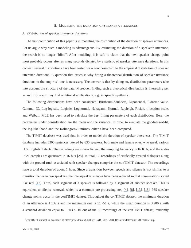
II. M ODELING THE DURATION OF SPEAKER UTTERANCES

A. Distribution of speaker utterance durations

The first contribution of this paper is in modeling the distribution of the duration of speaker utterances.

Let us argue why such a modeling is advantageous. By estimating the duration of a speaker’s utterance,

the search is no longer “blind”. After modeling, it is safe toclaim that the next speaker change point

most probably occurs after as many seconds dictated by a statistic of speaker utterance durations. In this

context, several distributions have been tested for a goodness-of-fit to the empirical distribution of speaker

utterance durations. A question that arises is why fitting a theoretical distribution of speaker utterance

durations to the empirical one is necessary. The answer is that by doing so, distribution parameters take

into account the structure of the data. Moreover, finding sucha theoretical distribution is interesting per

se and this result may find additional applications, e.g. in speech synthesis.

The following distributions have been considered: Birnbaum-Saunders, Exponential, Extreme value,

Gamma, IG, Log-logistic, Logistic, Lognormal, Nakagami, Normal, Rayleigh, Rician, t-location scale,

and Weibull. MLE has been used to calculate the best fitting parameters of each distribution. Here, the

parameters under consideration are the mean and the variance. In order to evaluate the goodness-of-fit,

the log-likelihood and the Kolmogorov-Smirnov criteria have been computed.

The TIMIT database was used first in order to model the duration ofspeaker utterances. The TIMIT

database includes 6300 sentences uttered by 630 speakers, both male and female ones, who speak various

U.S. English dialects. The recordings are mono-channel, the sampling frequency is 16 KHz, and the audio

PCM samples are quantized in 16 bits [28]. In total, 55 recordings of artificially created dialogues along

with the ground-truth associated with speaker changes comprise the conTIMIT dataset.1 The recordings

have a total duration of about 1 hour. Since a transition between speech and silence is not similar to a

transition between two speakers, the inter-speaker silences have been reduced so that conversations sound

like real [12]. Thus, each segment of a speaker is followed by asegment of another speaker. This is

equivalent to silence removal, which is a common pre-processing step [4], [8], [13], [15]. 935 speaker

change points occur in the conTIMIT dataset. Throughout the conTIMIT dataset, the minimum duration

of an utterance is 1.139 s and the maximum one is 11.751 s, while the mean duration is 3.286 s with

a standard deviation equal to 1.503 s. 10 out of the 55 recordings of the conTIMIT dataset, randomly

1conTIMIT dataset is available at http://poseidon.csd.auth.gr/LABRESEARCH/Latest/data/conTIMITdataset.zip

March 22, 2008 DRAFT

7

chosen, were used to create the conTIMIT training-1 dataset,employed in modeling the speaker utterance

duration.

IG distribution has been found to be the best fit with respect toboth log-likelihood and Kolmogorov-

Smirnov test. The values of mean utterance duration and standard deviation for the conTIMIT training-1

dataset under the IG model equal 3.286 s and 1.388 s, respectively. An illustration of the best fit for

the aforementioned distributions to the empirical distribution of speaker utterance durations can be seen

in Figure 2 with respect to the probability-probability (P-P) plots. Let us denote the mean and the

standard deviation of durations byµ and σ. Let Fk(·) be thekth normalized theoretical cumulative

density function (cdf) tested. To make a P-P plot, uniform quantiles qi = iN+1 , i = 1, 2, . . . , N , are

defined in the horizontal axis, whereN is the number of the samples whose distribution is estimated.

The vertical axis represents the value admitted by the theoretical cdf at t(i)−µ

σ, i.e. Fk(

t(i)−µ

σ), wheret(i)

is the ith order statistic of utterance durations. That is, the durations are arranged in an increasing order

and theith sorted value is chosen. The better the theoretical cdf approximates the empirical one, the

closer the points (qi, Fk(t(i)−µ

σ)) are to the diagonal [29].

To validate that IG distribution generally fits best the empirical speaker utterance duration distribution,

another dataset has been employed, to be referred to as the movie dataset [30]. In this dataset, 25 audio

recordings are included that have been extracted from six movies of different genres, namely: Analyze

That, Cold Mountain, Jackie Brown, Lord of the Rings I, Platoon,and Secret Window. Indeed, Analyze

That is a comedy, Platoon is an action, and Cold Mountain is a drama. Thus, dialogues of different natures

are included in the movie dataset. Speaker segmentation has been performed by human agents. Having the

ground-truth speaker change points, the distribution of speaker utterance duration for the movie dataset

is modeled by applying the same procedure as for the conTIMIT training-1 dataset. The best fit is found

to be the IG distribution, once again, with respect to both log-likelihood and Kolmogorov-Smirnov test.

This outcome is of great importance, since the dialogues are not recorded in a clean environment. Longer

pauses or overlaps between the actor utterances exist and background music or noise occurs. However, as

expected, different parameters from those estimated in theconTIMIT training-1 dataset are obtained. In

the movie dataset, the mean duration equals 5.333 s, while the standard deviation is 6.189 s. Accordingly,

modeling the duration of speaker utterances by an IG distribution helps to predict the next speaker change

point.

March 22, 2008 DRAFT

8

qi

F(x

(i)−

µ

σ)

duration (sec)

Birnbaum-SaundersExponentialExtreme valueGamma

120

0 0.2 0.4 0.6 0.8 10

0.1

0.2

0.3

0.4

0.5

0.6

0.7

0.8

0.9

1

(a)

qi

F(t (

i)−

µ

σ)

duration (sec)

Inverse GaussianLog-LogisticLogistic

120

0 0.2 0.4 0.6 0.8 10

0.1

0.2

0.3

0.4

0.5

0.6

0.7

0.8

0.9

1

(b)

qi

F(t (

i)−

µ

σ)

duration (sec)

LognormalNakagamiNormalReyleich

0 12

0 0.2 0.4 0.6 0.8 10

0.1

0.2

0.3

0.4

0.5

0.6

0.7

0.8

0.9

1

(c)

qi

F(t (

i)−

µ

σ)

duration (sec)

Riciant location-scaleWeibull

0 12

0 0.2 0.4 0.6 0.8 10

0.1

0.2

0.3

0.4

0.5

0.6

0.7

0.8

0.9

1

(d)

Fig. 2. (a) The P-P plots for distributions Birnbaum-Saunders, Exponential, Extreme value, Gamma for the conTIMIT training-1dataset. (b) The P-P plots for distributions IG, Log-Logistic, Logistic for the conTIMIT training-1 dataset. (c) The P-P plots fordistributions Lognormal, Nakagami, Normal, Reyleigh for the conTIMIT training-1 dataset. (d) The P-P plots for distributionsRician, t-location scale, Weibull for the conTIMIT training-1 dataset.

B. Mathematical properties of the IG distribution and its application

Some of the main mathematical properties of the IG distribution are briefly discussed next. The IG

distribution, or Wald distribution, has probability density function (pdf) with parametersµ andλIG [31],

[32]:

f(t) =

√λIG

2πt3exp

(−λIG(t − µ)2

2µ2t

)t ∈ (0,∞) (1)

March 22, 2008 DRAFT

9

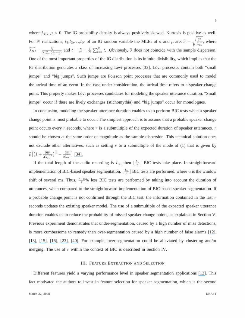
whereλIG, µ > 0. The IG probability density is always positively skewed. Kurtosis is positive as well.

For N realizations,t1,t2,. . .,tN of an IG random variable the MLEs ofσ andµ are: σ =

√t3

λIG

, where

λIG = N∑N

i=1(1

ti

− 1

t)

and t = µ = 1N

∑Ni=1 ti. Obviously,σ does not coincide with the sample dispersion.

One of the most important properties of the IG distribution is its infinite divisibility, which implies that the

IG distribution generates a class of increasing Levi processes [33]. Levi processes contain both “small

jumps” and “big jumps”. Such jumps are Poisson point processesthat are commonly used to model

the arrival time of an event. In the case under consideration, the arrival time refers to a speaker change

point. This property makes Levi processes candidates for modeling the speaker utterance duration. “Small

jumps” occur if there are lively exchanges (stichomythia) and “big jumps” occur for monologues.

In conclusion, modeling the speaker utterance duration enables us to perform BIC tests when a speaker

change point is most probable to occur. The simplest approachis to assume that a probable speaker change

point occurs everyr seconds, wherer is a submultiple of the expected duration of speaker utterances.r

should be chosen at the same order of magnitude as the sample dispersion. This technical solution does

not exclude other alternatives, such as settingr to a submultiple of the mode of (1) that is given by

µ[(

1 + 9µ2

4λIG

2

) 1

2 − 3µ

2λIG

][34].

If the total length of the audio recording isLa, then ⌊La

r⌋ BIC tests take place. In straightforward

implementation of BIC-based speaker segmentation,⌊La

u⌋ BIC tests are performed, whereu is the window

shift of several ms. Thus,r−ur

% less BIC tests are performed by taking into account the duration of

utterances, when compared to the straightforward implementation of BIC-based speaker segmentation. If

a probable change point is not confirmed through the BIC test, the information contained in the lastr

seconds updates the existing speaker model. The use of a submultiple of the expected speaker utterance

duration enables us to reduce the probability of missed speaker change points, as explained in Section V.

Previous experiment demonstrates that under-segmentation, caused by a high number of miss detections,

is more cumbersome to remedy than over-segmentation causedby a high number of false alarms [12],

[13], [15], [16], [23], [40]. For example, over-segmentation could be alleviated by clustering and/or

merging. The use ofr within the context of BIC is described in Section IV.

III. F EATURE EXTRACTION AND SELECTION

Different features yield a varying performance level in speaker segmentation applications [13]. This

fact motivated the authors to invest in feature selection for speaker segmentation, which is the second

March 22, 2008 DRAFT

10

contribution of the paper.

MFCCs, sometimes with their first-order (delta) and/or second-order differences (delta-delta) are the

most commonly used features in speaker segmentation. Furthermore, MFCCs were used in various

techniques besides BIC such as HMMs [9] or SVMs [10]. Still, notall the researchers employ the

same MFCC order in BIC-based approaches. For example, 24 MFCCsare employed in [7], while 12

MFCCs and their first differences are utilized in [12] and [20].32 MFCCs are used in [11]. In [4], 16

MFCCs are applied, while 12 MFCCs along with their delta and delta-delta coefficients are employed

in [9]. 23 MFCCs are utilized in [1], [8] and 24 MFCCs are appliedin [5], [15], [18]. A more detailed

study is presented in [22], where a comparative study between 12 MFCCs, 13 MFCCs and their delta

coefficients, and 13 MFCCs, their delta, and delta-delta coefficients is performed.

A different approach is investigated here. Instead of trying to reveal the MFCC order that yields the

most accurate speaker turn point detection results, an effort is made to find out an MFCC subset that is

more suitable for detecting a speaker change. The MFCCs are calculated every 10 ms with 62.5% overlap

by the algorithm described in [35]. An initial set consisting of 36 MFCCs is formed and the goal is to

derive the subset, which contains the 24 more suitable MFCCs for speaker segmentation, since utilizing

24 coefficients is commonplace in [5], [15], [18].

Let us test the hypothesis there is a speaker change point against the hypothesis there is no speaker

change point. Speakers change once under the first hypothesis,while a monologue is observed under

the second one. For training purposes, an additional dataset of 50 recordings was created from speaker

utterances derived in the TIMIT database, referred to as the conTIMIT training-2 dataset, that is disjoint

to the conTIMIT dataset2. 25 out of the 50 recordings contain a speaker change point and the remaining

25 recordings do not. In this way, two classes are presumed: the first class represents a speaker change

and includes 25 recordings with one speaker change and the second class corresponds to no speaker

changes and includes 25 recordings with monologues. We assume that the mean feature vectors in the

two different classes are different in order to enable discrimination [24]. The goal of feature selection

is to find a feature subsetFi(D) of dimensionD. In our case,D = 24. Let J denote the performance

measure. Feature selection findsFi(D) such thatJ(Fi(D)) ≥ J(Fj(D)), wherej ∈ 1, . . . , q(D) and

2conTIMIT training-2 dataset is available at http://poseidon.csd.auth.gr/LAB RESEARCH/Latest/data/conTIMITtraining-2dataset.zip

March 22, 2008 DRAFT

11

q(D) is the number of distinguishable subsets containingD elements. If 24 out of the 36 coefficients are

to be selected, thenq(24)=

(36

24

)is enormous. As a result, a more efficient search strategy thanexhaustive

search is required. Such an alternative is branch and bound, which attains an almost optimal performance

[24]. The search process is accomplished systematically by means of a tree structure consisting of 36-

24+1=13 levels. A level is composed of a number of nodes and each node corresponds to a coefficient

subset. At the highest level, there is only one node corresponding to the full set of coefficients. At the

lowest level, there are nodes containing 24 coefficients. The search process starts from the highest level

by systematically traversing all levels until the lowest level is reached. The traversing algorithm uses

depth-first search with a backtracking mechanism. This means that if J1 is the best performance found

so far, then branches whose performance is worse thanJ1 are skipped [24].

The selection criterionJ can be defined in terms of scatter matrices. A scatter matrix gives information

about the dispersion of samples around their mean. The within-class scatter matrix,Sw, describes the

within-class dispersion. The between-class scatter matrix, Sb, describes the dispersion of the class-

dependent sample means around the gross mean. Mathematically, J is defined by

J = tr(S−1w Sb) (2)

wheretr(·) stands for the matrix trace operator. J, as defined in (2), is a monotonically increasing function

of the distance between the mean vectors and a monotonicallydecreasing function of the scattering around

the mean vectors. Moreover, (2) is invariant to reversible linear transformations. In addition, it is ideal

for Gaussian distributed feature vectors. To a first approximation, MFCCs are assumed to follow the

Gaussian distribution. Under this assumption, (2) guarantees the best performance [24].

From each recording, 36-order MFCCs are extracted. The selected 24 MFCCs for the conTIMIT

training-2 dataset can be seen in Table I. Although the selection of MFCCs, as in Table I, might depend

on the dataset used for feature selection, the aforementioned feature selection can be applied to any

dataset. MFCCs shown in Table I are used in conjunction with their delta and delta-delta coefficients,

in order to capture their temporal evolution that carries additional useful information. In general, the

temporal evolution is found to increase efficiency [9], [15],[20], [22]. However, in [12], it is reported

that using delta and delta-delta coefficients impairs efficiency.

Alternatively, one could replace (2) with BIC (5) itself. Then feature selection is performed by a

March 22, 2008 DRAFT

12

TABLE ITHE SELECTED24 MFCCS FOR THE CONTIMIT TRAINING-2 DATASET.

# 1 2 3 4 5 6 7 8 9 10 11 12MFCC 1st 3rd 4th 5th 6th 7th 8th 9th 10th 11th 13th 16th

# 13 14 15 16 17 18 19 20 21 22 23 24MFCC 22th 23th 24th 25th 26th 27th 28th 29th 31th 33th 35th 36th

wrapper instead of a filter [36], as (2) implies. In such case, the selected MFCCs are: : 1st-18th, 22nd,

23rd, 27th, 28th, 31st, and 35th. The computation time required by (2) is less by 187.06% than that

required by BIC, when a PC with a 3 GHz Athlon processor and 1 GB of RAM is used. In Section V,

we comment on the accuracy of the latter feature selection method.

IV. BIC- BASED SPEAKER SEGMENTATION

In this section, the BIC criterion is detailed and an equivalent BIC criterion is derived, that is consid-

erably less computationally demanding. It is also explained how the contributions of Sections II and III

are utilized in conjunction with BIC.

BIC is a maximum likelihood, asymptotically optimal, Bayesian model selection criterion penalized

by the model complexity. For speaker turn detection, two different models are employed. Assume that

there are two neighboring chunksX and Y around timetj . The problem is to decide whether or not

a speaker change point exists attj . Let Z = X ∪ Y and NX , NY , NZ be the numbers of samples in

chunksX, Y , and Z, respectively. Obviously,NY = NZ − NX . The problem is formulated as a two

hypothesis testing problem.

Under H0 there is no speaker change point at timetj . MLE is used to compute the parameters of

a Gaussian distribution that models the data samples inZ. Let us denote byθZ the parameters of the

Gaussian distribution, i.e. the mean vectorµZ and the full covariance matrixΣZ . The log-likelihoodL0

underH0 is

L0 =

NX∑

i=1

ln p(zi|θZ) +

NZ∑

i=NX+1

ln p(zi|θZ) (3)

wherezi ∈ Rd, i = 1, 2, . . . , NZ which are assumed to be independent.zi consists of the 24 selected

MFCCs with their delta and delta-delta coefficients, i.e.d = 72. Under H1 there is a speaker change

point at timetj . The chunksX and Y are modeled by distinct multivariate Gaussian densities, whose

March 22, 2008 DRAFT

13

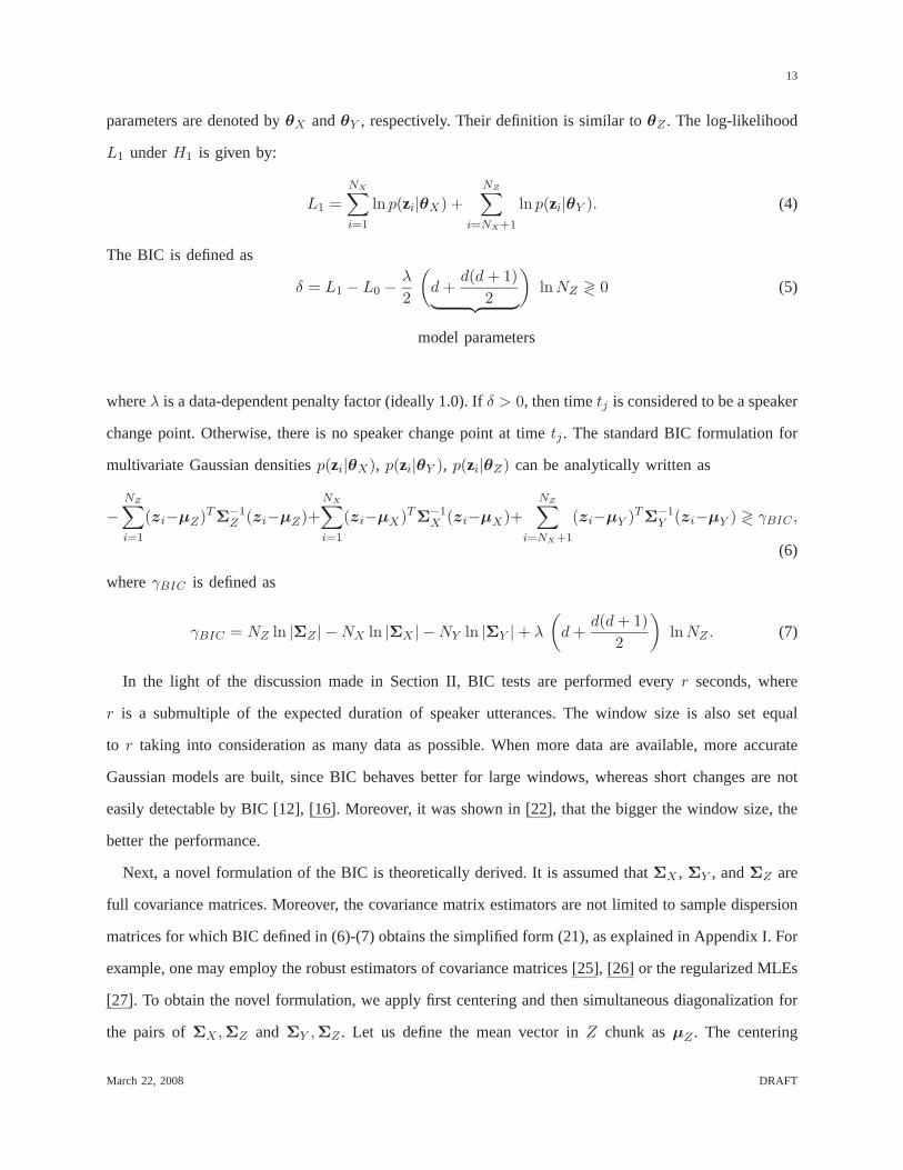
parameters are denoted byθX andθY , respectively. Their definition is similar toθZ . The log-likelihood

L1 underH1 is given by:

L1 =

NX∑

i=1

ln p(zi|θX) +

NZ∑

i=NX+1

ln p(zi|θY ). (4)

The BIC is defined as

δ = L1 − L0 −λ

2

(d +

d(d + 1)

2︸ ︷︷ ︸

)lnNZ ≷ 0 (5)

model parameters

whereλ is a data-dependent penalty factor (ideally 1.0). Ifδ > 0, then timetj is considered to be a speaker

change point. Otherwise, there is no speaker change point attime tj . The standard BIC formulation for

multivariate Gaussian densitiesp(zi|θX), p(zi|θY ), p(zi|θZ) can be analytically written as

−

NZ∑

i=1

(zi−µZ)TΣ

−1Z (zi−µZ)+

NX∑

i=1

(zi−µX)TΣ

−1X (zi−µX)+

NZ∑

i=NX+1

(zi−µY )TΣ

−1Y (zi−µY ) ≷ γBIC ,

(6)

whereγBIC is defined as

γBIC = NZ ln |ΣZ | − NX ln |ΣX | − NY ln |ΣY | + λ

(d +

d(d + 1)

2

)lnNZ . (7)

In the light of the discussion made in Section II, BIC tests areperformed everyr seconds, where

r is a submultiple of the expected duration of speaker utterances. The window size is also set equal

to r taking into consideration as many data as possible. When more data are available, more accurate

Gaussian models are built, since BIC behaves better for large windows, whereas short changes are not

easily detectable by BIC [12], [16]. Moreover, it was shown in [22], that the bigger the window size, the

better the performance.

Next, a novel formulation of the BIC is theoretically derived. It is assumed thatΣX , ΣY , andΣZ are

full covariance matrices. Moreover, the covariance matrixestimators are not limited to sample dispersion

matrices for which BIC defined in (6)-(7) obtains the simplifiedform (21), as explained in Appendix I. For

example, one may employ the robust estimators of covariancematrices [25], [26] or the regularized MLEs

[27]. To obtain the novel formulation, we apply first centering and then simultaneous diagonalization for

the pairs ofΣX ,ΣZ and ΣY ,ΣZ . Let us define the mean vector inZ chunk asµZ . The centering

March 22, 2008 DRAFT

14

transformation iszi = zi − µZ . Next, simultaneous diagonalization ofΣX andΣZ is applied. LetΛZ

be the diagonal matrix of the eigenvalues ofΣZ andΦ be the corresponding modal matrix. Let us define

K = Λ− 1

2

Z ΦTΣXΦΛ

− 1

2

Z = ΨΛKΨT , whereΛK is the diagonal matrix of eigenvalues ofK andΨ is

the corresponding modal matrix. The simultaneous diagonalization transformation yields forzi ∈ Z ∩

X = X

wi = ΨTΛ

− 1

2

Z ΦT zi. (8)

Let H = ΛZ− 1

2 ΦTΣY ΦΛZ

− 1

2 and H = ΞΛHΞT . Following the same strategy, we obtain forzi ∈

Z ∩ Y = Y

vi = ΞTΛ

− 1

2

Z ΦT zi. (9)

In Appendix I, it is shown that (6) is equivalently rewrittenas

NX∑

i=1

wTi (ΛK

−1 − I)wi +

NZ∑

i=NX+1

vTi (ΛH

−1 − I)vi ≷ γ′ (10)

whereγ′ is an appropriate threshold derived analytically in (26).

Concerning the computational cost, simultaneous diagonalization replaces matrix inversions and simpli-

fies the quadratic forms to be computed. This leads to a substantially less computational costly transformed

BIC, as opposed to the standard BIC. As it is detailed in Appendix II, the computational cost of the

standard BIC in flops, excluding the cost ofγBIC , is

3d3 + 6NZd2 + (8NZ + 3)d + 2, (11)

whereas the computational cost of the transformed BIC, excluding the cost ofγBIC , equals

30d3 + (4NZ + 4)d2 + (7NZ + 9)d + 5. (12)

Sinced ≪ NZ , by comparing (11) and (12), it can be seen that the standard BIC is more computationally

costly than its transformed alternative.

To sum up, the algorithm can be roughly sketched as follows:

1) Initialize the interval[a, b] to [0, 2r] and letv = a+b2 .

2) Until the audio recording end, use BIC with the selected MFCCs to evaluate if there is a change

point in [a, b].

March 22, 2008 DRAFT

15

3) If there is no speaker change point in[a, b], thenb = b + r. Go to step 2).

4) If there is a speaker change point in[a, b], thena = v, b = v + r. Go to step 2).

It is reminded thatr is a submultiple of the mean utterance duration, which is obtained by the analysis in

Section II and the term selected MFCCs refers to the MFCCs chosenby the feature selection algorithm,

described in Section III.

V. EXPERIMENTAL RESULTS AND DISCUSSION

A. Figures of Merit

To judge the efficiency of speaker turn point detection algorithms, two sets of figures of merit are

commonly used. On the one hand, one may use the false alarm rate (FAR) and the miss detection rate

(MDR) defined as

FAR = FAGT+ FA

, MDR = MDGT

(13)

whereFA denotes the number of false alarms,MD the number of miss detections, andGT stands for

the number of actual speaker turns, i.e. the ground truth. A false alarm occurs when a speaker turn is

detected although it does not exist, while a miss detection occurs, when the process does not detect an

existing speaker turn [12], [23]. On the other hand, one may employ the precision (PRC), recall (RCL)

andF1 rates given by

PRC = CFCDET

= CFCCFC+FA

, RCL = CFCGT

= CFCCFC+MD

, F1 = 2 PRC RCLPRC+RCL

(14)

whereCFC denotes the number of correctly found changes andDET = CFC + FA is the number

of detected speaker changes.F1 admits a value between 0 and 1. The higher its value is, the better

performance is obtained [8], [18]. Between the pairs (FAR, MDR) and (PRC, RCL), the following

relationships hold:

MDR = 1 − RCL, FAR = RCL FADET PRC+RCL FA

. (15)

In order to facilitate a comparative assessment of our results with others reported in the literature, the

evaluation of the proposed approach is carried out using allthe aforementioned figures of merit.

March 22, 2008 DRAFT

16

B. Evaluation

1) Comparative performance evaluation on the conTIMIT test dataset: The total number of recordings

in the conTIMIT dataset is 55. The evaluation is performed upon49 randomly selected recordings of

the conTIMIT dataset, forming the conTIMIT test dataset. The remaining 6 were used to determine the

value of the BIC penalty-factorλ and to create the conTIMIT training-3 dataset. Although the conTIMIT

dataset is an artificially created dataset and includes no real conversations, performance assessment over

the conTIMIT test dataset is still informative. It is also reminded that 10 randomly chosen recordings out

of the 55 ones of the conTIMIT dataset, are employed to model the speaker utterance duration (conTIMIT

training-1 dataset). Consequently, there is a partial overlap between the conTIMIT test dataset and the

conTIMIT training-1 dataset. It has been reported that BIC performance is likely to reach a limit [20].

There are 4 reasons for that: (a) estimates of the BIC model parameters are used, (b) the penalty-factor

λ may not be tuned properly, (c) the data are assumed to be jointly normal, but this is an assumption,

frequently not validated, for example when voiced speech isembedded into noise [37], and (d) researchers

have found that BIC faces problems for small sample sets [37], [38]. Researchers tend to agree that BIC

performance deteriorates when a speaker utterance does nothave sufficient duration, which should be

more than about 2 s. For the conTIMIT test dataset, the tolerance equals 1 s. That is, 0.5 s before and

after the actual speaker change point.

For evaluation purposes, 4 systems are assessed, namely: (a) The BIC system without speaker utterance

duration estimation and feature selection. This is the baseline system (system 1). (b) The BIC system with

speaker utterance duration estimation (system 2). (c) The BIC system with feature selection (system 3).

(d) The proposed system, that is the BIC system with speaker utterance duration estimation and feature

selection (system 4). The window shiftr is set equal to the half of the average speaker utterance duration

for systems 2 and 4, whereasr is equal to 0.2 s for systems 1 and 3.

BIC performance on the conTIMIT test dataset without modeling the speaker utterance duration and

feature selection is depicted in Table II. The performance ofBIC with modeling the distribution of the

speaker utterance is exhibited in Table III, while its performance when feature selection is applied only

is summarized in Table IV. The overall performance of the proposed system (system 4) is summarized

in Table V. For all systems, the figures of merit are computed for each audio recording and then their

corresponding mean value and standard deviation are reported [43]. Concerning system 4, if (2) is replaced

March 22, 2008 DRAFT

17

TABLE IIPERFORMANCE OFBIC ON THE CONTIMIT TEST DATASET

WITHOUT MODELING THE SPEAKER UTTERANCE DURATION

NOR APPLYING FEATURE SELECTION.

PRC RCL F1 FAR MDR

mean 0.446 0.647 0.516 0.352 0.353standard deviation 0.094 0.137 0.081 0.157 0.137

TABLE IIIPERFORMANCE OFBIC ON THE CONTIMIT TEST DATASET

WITH MODELING THE SPEAKER UTTERANCE DURATION.

PRC RCL F1 FAR MDR

mean 0.613 0.895 0.723 0.311 0.105standard deviation 0.079 0.116 0.077 0.114 0.116

TABLE IVPERFORMANCE OFBIC ON THE CONTIMIT TEST DATASET

WITH FEATURE SELECTION.

PRC RCL F1 FAR MDR

mean 0.527 0.654 0.567 0.295 0.335standard deviation 0.159 0.137 0.110 0.177 0.150

TABLE VPERFORMANCE OF THE PROPOSED SYSTEM ON THE

CONTIMIT TEST DATASET SYSTEM(WITH MODELING THE

SPEAKER UTTERANCE DURATION AND FEATURE SELECTION).

PRC RCL F1 FAR MDR

mean 0.670 0.949 0.777 0.289 0.051standard deviation 0.106 0.056 0.069 0.139 0.056

by BIC, it is found thatPRC=0.685,RCL= 0.951,F1=0.974,FAR= 0.303, andMDR=0.049. However,

it is reminded that the improvement is achieved at the cost ofconstraining the generalization ability.

Our aim is to validate that each system differentiates significantly from the others concerning their

mean figures of merit. First, one-way analysis of variance (one-way ANOVA) is applied. The null

hypothesis tested is that the 4 system mean figures of merit areequal. The alternative hypothesis states

that the differences among the figures of merit are not due to random errors, but due to variation among

unequal mean figures of merit. That is, the null hypothesis declares that the systems do not differentiate

significantly from one another, while the alternative hypothesis suggests that at least one of the systems

differs from the remaining. The F-statistic value and its p-value for all five efficiency measures are

indicated in Table VI. From Table VI, it is evident that the 4 systems are statistically different, with

TABLE VIF-STATISTIC VALUES AND P-VALUES FORPRC , RCL, F1, FAR, AND MDR OF THE 4 SYSTEMS TESTED ON THE

CONTIMIT TEST DATASET.

PRC RCL F1 FAR MDR

F-statistic 36.322 90.295 103.931 1.794 81.576p-value 1.945 10−6 2.743 10−8 1.009 10−9 0.150 9.324 10−7

respect toPRC, RCL, F1, and MDR, whereas there appears to be no significant difference with

respect to theFAR at 95% confidence level.

March 22, 2008 DRAFT

18

TABLE VII95%CONFIDENCE INTERVALS FOR ALL PAIRWISE

COMPARISONS OF THE4 SYSTEMS FORPRC .

systems compared 95% confidence interval1st - 2nd [-0.224,-0.107]1st - 3rd [-0.140,-0.022]1st - 4th [-0.282,-0.164]2nd - 3rd [0.027,0.145]2nd - 4th [-0.116,-0.002]3rd - 4th [-0.201,-0.083]

TABLE VIII95%CONFIDENCE INTERVALS FOR ALL PAIRWISE

COMPARISONS OF THE4 SYSTEMS FORRCL.

systems compared 95% confidence interval1st - 2nd [-0.309,-0.188]1st - 3rd [-0.067,-0.054]1st - 4th [-0.363,-0.241]2nd - 3rd [0.181,0.302]2nd - 4th [-0.114,-0.007]3rd - 4th [-0.356,-0.235]

One-way ANOVA assures us that at least one system is different from the others. However no

information is provided about the pairs of systems that differentiate. Tukey’s method or honestly significant

difference method is applied to find the pairs of systems that differentiate [39]. Tukey’s method is designed

to make all pairwise comparisons of means, while maintaining the confidence level at a pre-defined level.

Moreover, it is optimal for balanced one-way ANOVA, which isour scenario. Fork systems, there are

k

(k−12

)possible combinations (e.g. 6 possible combinations are examined fork = 4). Tukey’s method

for the same number of measurements is applied, i.e. 49. The critical test statistic is obtained from the

Studentized range statistic.

Since one-way ANOVA has validated thatFAR differences are not significant, Tukey’s method is

applied to the remaining figures of merit i.e.PRC, RCL, F1, andMDR for the same confidence level

95%. The corresponding confidence intervals for all pairwise comparisons among the 4 systems for the

aforementioned figures of merit can be seen in Tables VII - X, respectively. If the confidence interval

includes zero, the difference is not significant. It is clear from Tables VII - X that zero is not included in

any interval. Thus, for any pairwise system comparison and any figure of merit fromPCR, RCL, F1,

andMDR the difference is significant.

Accordingly, there is statistical evidence that both speaker utterance modeling and feature selection

improve performance significantly either individually or combinedfor PRC, RCL, F1 andMDR. This

is not the case forFAR.

2) MDR histogram of the conTIMIT test dataset:We focus on the results of the proposed system for

the conTIMIT test dataset depicted in Table V. TheMDR histogram is plotted in Figure 3. A clear peak

exists near to 0, which is the ideal case. The latter is a directoutcome of the fact that two-hypothesis

BIC tests are carried out at times, where a speaker change point is most probable to occur.

March 22, 2008 DRAFT

19

TABLE IX95%CONFIDENCE INTERVALS FOR ALL PAIRWISE

COMPARISONS OF THE4 SYSTEMS FORF1.

systems compared 95% confidence interval1st - 2nd [-0.251,-0.162]1st - 3rd [-0.095,-0.006]1st - 4th [-0.307,-0.218]2nd - 3rd [0.112,0.201]2nd - 4th [-0.101,-0.012]3rd - 4th [-0.257,-0.168]

TABLE X95%CONFIDENCE INTERVALS FOR ALL PAIRWISE

COMPARISONS OF THE4 SYSTEMS FORMDR.

systems compared 95% confidence interval1st - 2nd [0.186,0.311]1st - 3rd [-0.044,-0.081]1st - 4th [0.240,0.364]2nd - 3rd [-0.292,-0.168]2nd - 4th [-0.009,-0.116]3rd - 4th [0.221,0.346]

MDR

freq

uenc

y

0 0.02 0.04 0.06 0.08 0.1 0.12 0.14 0.16 0.180

5

10

15

20

25

Fig. 3. The histogram ofMDR in the conTIMIT test dataset.

3) Correlation among figures of merit on the conTIMIT test dataset: The correlation coefficient

between the figures of merit for the conTIMIT test dataset can beseen in Table XI. The correlation

coefficient betweenRCL andMDR is -1, as a consequence of (15). The pairs: (i) (PRC, RCL) and

(PRC, MDR) (ii) (F1, RCL) and (F1, MDR) (iii) ( FAR, RCL) and (FAR, MDR) have opposite

signs. That is, when the first quantity increases, the second decreases and vice versa. The degree of linear

dependence is indicated by the absolute value of the correlation index. It is seen that (PRC,F1) and

(PRC,FAR) exhibit the strongest correlation.

TABLE XITHE CORRELATION COEFFICIENT BETWEEN THE PAIRS OF FIGURES OF MERIT FOR THE CONTIMIT TEST DATASET.

PRC RCL F1 FAR MDR

PRC 1 -0.344 0.939 -0.945 0.344RCL 1 -0.014 0.628 -1F1 1 -0.778 0.014FAR 1 -0.628MDR 1

March 22, 2008 DRAFT

20

4) Performance evaluation on the HUB-4 1997 English Broadcast News Speech dataset:Aiming

to verify the efficiency of the proposed contributions, i.e. modeling the speaker utterance duration and

feature selection on real data, RT-03 MDE Training Data Speech is utilized [44]. To facilitate performance

comparisons between the proposed system and other systems,we confine ourselves to broadcast news

audio recordings, that is the HUB-4 1997 English Broadcast News Speech dataset [41]. The recordings

are mono-channel, the sampling frequency is 16 KHz, and the audio PCM samples are quantized in 16

bits. The selected audio recordings have a duration of approximately 1 hour.

20% of the selected audio recordings are used for estimatingthe speaker utterance duration distribution.

For the third time, IG distribution is verified to be the best fit for modeling speaker utterance duration

by both the log-likelihood and the Kolmogorov-Smirnov criteria. In this case, the mean duration equals

23.541 s and the standard deviation equals 24.210 s. Since thestandard deviation value is considerably

large,r is set equal to one eighth of the mean speaker utterance duration. This rather small submultiple

aims to reduce the probability of missing a speaker change for the reasons explained in Section II-B.

To assess the robustness of the MFCCs shown in Table I, the samecoefficients along with their

corresponding delta and delta-delta coefficients have been used in the HUB-4 1997 English Broadcast

News Speech dataset. The proposed algorithm is tested on the remaining 80% of the selected audio

recordings. For the HUB-4 1997 English Broadcast News Speech dataset, since the dialogues are real,

the tolerance should be greater, as is explained in [12]. Motivated by [23], that also employs broadcasts,

the tolerance is equal to 2 s. The achieved figures of merit are:PRC = 0.634, RCL = 0.922, F1 = 0.738,

FAR = 0.309, andMDR = 0.078.

5) Performance discussion:Before discussing the performance of the proposed system with respect to

other systems, let us argue why it is generally a good choice to minimizeMD even if FA is high [12].

FA can be more easily removed [13], [15], [16], [40], for example through clustering.PRC andFAR

are associated withFA, while RCL andMDR depend onMD. This means thatPRC andFAR are

less cumbersome to remedy thanRCL andMDR.

The proposed system is evaluated on the conTIMIT test dataset first. It outperforms three other systems

tested on a similar dataset, created by concatenating speakers from the TIMIT database, as described

in [21]. Although the dataset in [21] is substantially smaller than the conTIMIT test dataset, the nature

of the audio recordings is the same enabling us to conduct fair comparisons. The performance achieved

March 22, 2008 DRAFT

21

by the previous approaches is summarized in Table XII. Missing entries are due to the fact that not all

researchers use the same set of figures of merit, which createsfurther implications in direct comparisons.

PRC andFAR of the proposed system on the conTIMIT test dataset are slightly deteriorated than those

obtained by the multiple pass system with a fusion scheme when speakers are modeled by quasi-GMMs

system. However,RCL and MDR are substantially improved.RCL and MDR are also improved

with respect to the two remaining systems. Finally, the superiority of the proposed system against the

three systems developed in [21] is demonstrated by the fact that its F1 value is relatively improved

by 7.917%, 6.438%, and 28.007%, respectively. In [12], the used dataset was created by concatenating

TABLE XIIAVERAGE FIGURES OF MERIT IN[12] AND [21] ON A SIMILAR DATASET CREATED BY CONCATENATING SPEAKERS FROM

THE TIMIT DATABASE.

system Database used PRC RCL F1 FAR MDR

Proposed system concatenated utterances from speakers of theTIMIT database (not the same concatenationas in [12])

0.670 0.949 0.777 0.289 0.051

Multiple pass systemwith a fusion scheme[21]

concatenated utterances from speakers of theTIMIT database

0.780 0.700 0.720 0.218 0.305

Speakers modeled byquasi-GMMs system[21]

concatenated utterances from speakers of theTIMIT database

0.680 0.800 0.730 0.280 0.200

Auxiliary second-orderand T 2 Hotelling statisticsystem[21]

concatenated utterances from speakers of theTIMIT database

0.490 0.812 0.607 0.455 0.188

Delacourt and Wellekens[12]

concatenated utterances from speakers of theTIMIT database

0.282 0.156

speaker utterances from the TIMIT database, too. However, this concatenation is not the same to the one

employed here. AlthoughFAR is slightly better that ours, the reportedMDR for the proposed system

is considerably lower. The relativeMDR improvement equals67.308%.

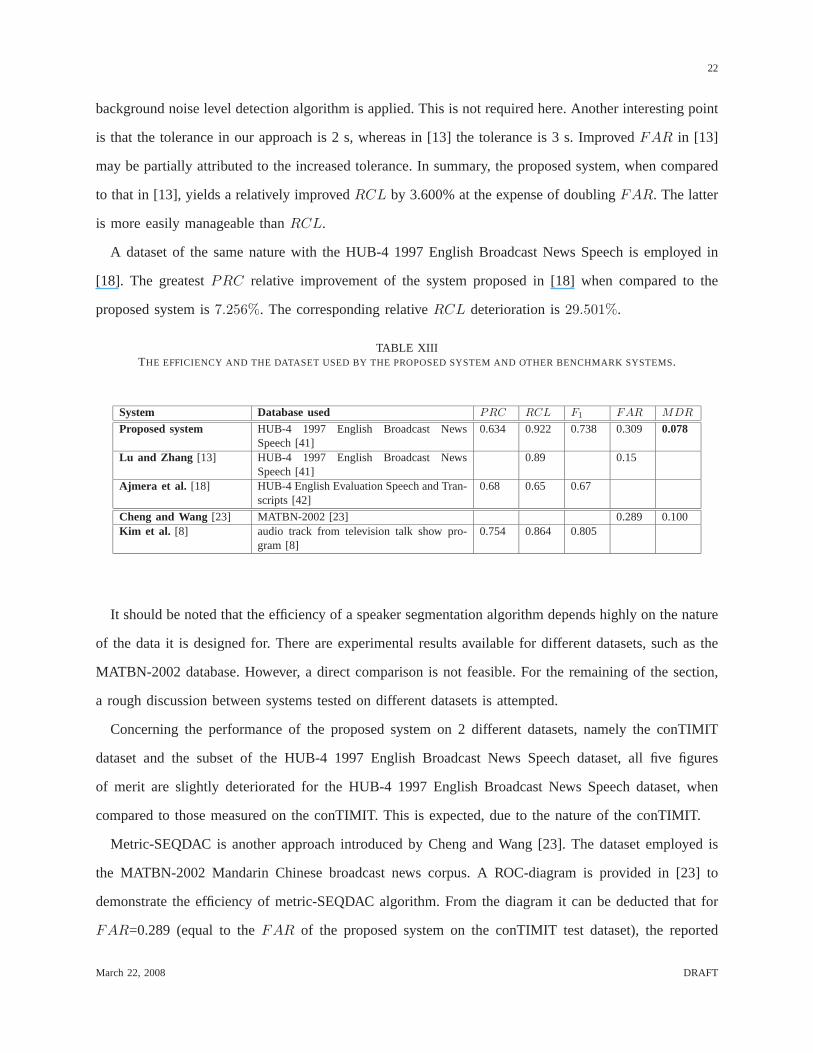
The proposed system is also assessed on the HUB-4 1997 English Broadcast News Speech dataset.

As is demonstrated in Table XIII, the same dataset is utilized in [13]. The system presented in [13] is a

two-step system. The first step is a ”coarse to refine” step, whereas the second step is a refinement one

that aims at reducingFAR. Both our algorithm and the one in [13] apply incremental speaker model

updating to deal with the problem of insufficient data in estimating the speaker model. However, the

updating strategy is not the same. In [13], quasi-GMMs are utilized. Both algorithms considerFAs less

cumbersome thanMDs. In [13], down-sampling takes place from 16 KHz to 8 KHz and an adaptive

March 22, 2008 DRAFT

22

background noise level detection algorithm is applied. Thisis not required here. Another interesting point

is that the tolerance in our approach is 2 s, whereas in [13] the tolerance is 3 s. ImprovedFAR in [13]

may be partially attributed to the increased tolerance. In summary, the proposed system, when compared

to that in [13], yields a relatively improvedRCL by 3.600% at the expense of doublingFAR. The latter

is more easily manageable thanRCL.

A dataset of the same nature with the HUB-4 1997 English Broadcast News Speech is employed in

[18]. The greatestPRC relative improvement of the system proposed in [18] when compared to the

proposed system is7.256%. The corresponding relativeRCL deterioration is29.501%.

TABLE XIIITHE EFFICIENCY AND THE DATASET USED BY THE PROPOSED SYSTEM ANDOTHER BENCHMARK SYSTEMS.

System Database used PRC RCL F1 FAR MDR

Proposed system HUB-4 1997 English Broadcast NewsSpeech [41]

0.634 0.922 0.738 0.309 0.078

Lu and Zhang [13] HUB-4 1997 English Broadcast NewsSpeech [41]

0.89 0.15

Ajmera et al. [18] HUB-4 English Evaluation Speech and Tran-scripts [42]

0.68 0.65 0.67

Cheng and Wang[23] MATBN-2002 [23] 0.289 0.100Kim et al. [8] audio track from television talk show pro-

gram [8]0.754 0.864 0.805

It should be noted that the efficiency of a speaker segmentation algorithm depends highly on the nature

of the data it is designed for. There are experimental resultsavailable for different datasets, such as the

MATBN-2002 database. However, a direct comparison is not feasible. For the remaining of the section,

a rough discussion between systems tested on different datasets is attempted.

Concerning the performance of the proposed system on 2 different datasets, namely the conTIMIT

dataset and the subset of the HUB-4 1997 English Broadcast News Speech dataset, all five figures

of merit are slightly deteriorated for the HUB-4 1997 EnglishBroadcast News Speech dataset, when

compared to those measured on the conTIMIT. This is expected, due to the nature of the conTIMIT.

Metric-SEQDAC is another approach introduced by Cheng and Wang [23]. The dataset employed is

the MATBN-2002 Mandarin Chinese broadcast news corpus. A ROC-diagram is provided in [23] to

demonstrate the efficiency of metric-SEQDAC algorithm. From thediagram it can be deducted that for

FAR=0.289 (equal to theFAR of the proposed system on the conTIMIT test dataset), the reported

March 22, 2008 DRAFT

23

MDR is roughly equal to 0.100. Once again, a great relativeMDR improvement equal to28.205% is

achieved at the expense of a6.472% relativeFAR deterioration.

Kim et al. [8] presented a hybrid speaker-based segmentation, which combines metric-based and model-

based techniques. Audio track from a television talk show program is used to evaluate the performance.

Comparing the proposed system to the one in [8],PRC is relatively deteriorated by15.915%, while

RCL is relatively improved by6.713%.

To sum up, the proposed system demonstrates a very lowMDR compared to state-of-the-art systems.

VI. CONCLUSIONS

A novel efficient and robust approach for automatic BIC-basedspeaker segmentation is proposed.

Computational efficiency is achieved through the speaker utterance modeling and the transformed BIC for-

mulation, whereas robustness is attained by feature selection and application of BIC tests at appropriately

selected time stamps. The first contribution of the paper is in modeling the duration of speaker utterances.

As a result, computational needs are reduced in terms of timeand memory. The IG distribution is found

to be the best fit for the empirical distribution of speaker utterance duration. The second contribution

of the paper is in MFCC selection. The third contribution is in the new theoretical formulation of BIC

after centering and simultaneous diagonalization, whose computational complexity is less than that of the

standard BIC, when covariance matrix estimators other thanthe sample dispersion matrices are used.

In order to attest that speaker utterance duration modelingand feature selection yield more robust

systems, 4 systems are tested on the conTIMIT test dataset: the first utilizes the standard BIC approach,

the second applies speaker utterance duration estimation,the third employs feature selection, and the fourth

is the proposed system that combines all proposals made in this paper. One-way ANOVA and a posteriori

Tukey’s method confirm that the 4 systems, when compared pairwise, are significantly different from one

another forPRC, RCL, F1, and MDR. Accordingly, the proposed contributions either individually

or in combination improve performance. Moreover, to overcome the restrictions posed by the artificial

dialogues in the conTIMIT dataset, first experimental resultson the HUB-4 1997 English Broadcast News

Speech dataset have verified the robustness of the proposed system.

March 22, 2008 DRAFT

24

ACKNOWLEDGEMENT

M. Kotti was supported by the “Propondis” Public Welfare Foundation and E. Benetos by the “Alexan-

der S. Onassis” Public Benefit Foundation through scholarships.

APPENDIX I

A detailed proof of the new formulation of BIC follows. Assuming that the chunksX, Y , andZ are

modeled by Gaussian density functions, we define

A , −NX(d

2ln(2π) +

1

2ln |ΣZ |) −

1

2

NX∑

i=1

(zi − µZ)TΣ

−1Z (zi − µZ)

+NX(d

2ln(2π) +

1

2ln |ΣX |) +

1

2

NX∑

i=1

(zi − µX)TΣ

−1X (zi − µX),

(16)

B , −NY (d

2ln(2π) +

1

2ln |ΣZ |) −

1

2

NZ∑

i=NX+1

(zi − µZ)TΣ

−1Z (zi − µZ)

+NY (d

2ln(2π) +

1

2ln |ΣY |) +

1

2

NZ∑

i=NX+1

(zi − µY )TΣ

−1Y (zi − µY ).

(17)

Under these assumptions, (5) equals to

δ = A + B −λ

2

(d +

d(d + 1)

2

)lnNZ ≷ 0. (18)

If ΣX , ΣY , andΣZ are estimated by sample dispersion matrices, it is true that

NX∑

i=1

(zi − µZ)TΣ

−1Z (zi − µZ) = trΣ−1

Z

NX∑

i=1

(zi − µZ)(zi − µZ)T , (19)

NX∑

i=1

(zi − µX)TΣ

−1X (zi − µX) = trΣ−1

X

NX∑

i=1

(zi − µX)(zi − µX)T = dNX . (20)

So, (16) can be written as:A = −NX(d2 ln(2π) + 1

2 ln |ΣZ |) −12trΣ−1

Z

∑NX

i=1(zi − µZ)(zi − µZ)T

+NX(d2 ln(2π) + 1

2 ln |ΣX |) + d2NX . Applying the same estimation forB allows us to rewrite (18) as

−NZ

2ln |ΣZ | +

NX

2ln |ΣX | +

NY

2ln |ΣY | −

λ

2

(d +

d(d + 1)

2

)lnNZ ≷ 0, (21)

which according to (7) corresponds toγBIC ≶ 0.

March 22, 2008 DRAFT

25

If we apply simultaneous diagonalization toΣX andΣZ , thenΣZ = ΦΛZΦT , whereΛZ andΦ are

the diagonal matrix of eigenvalues and modal matrix ofΣZ , respectively. Moreover, letK=ΛZ− 1

2 ΦTΣX

ΦΛZ− 1

2 . ΛK is the diagonal matrix of eigenvalues ofK andΨ is the corresponding modal matrix, i.e.

ΛK = ΨTKΨ. W is defined asW , ΦΛZ

− 1

2 Ψ. It is straightforward to prove thatWTΣZW = I

and WTΣXW = ΛK . The same procedure for simultaneous diagonalization ofΣY and ΣZ takes

place. LetH = ΛZ− 1

2 ΦTΣY ΦΛZ

− 1

2 . Additionally, ΛH is the diagonal matrix of eigenvalues ofH

and Ξ is the corresponding modal matrix i.e.ΛH = ΞTHΞ. If Ω is defined asΩ , ΦΛZ

− 1

2 Ξ, it is

straightforward to prove thatΩTΣZΩ = I andΩ

TΣY Ω = ΛH . The transformed (21) isNX

2 ln |WΛKWT ||WWT |

+NY

2 ln |ΩΛHΩT ||ΩΩT | -λ

2

(d + d(d+1)

2

)lnNZ ≷ 0 or equivalently,

NX

2

d∑

i=1

lnλi(ΛK) +NY

2

d∑

i=1

lnλi(ΛH) −λ

2

(d +

d(d + 1)

2

)lnNZ ≷ 0, (22)

whereλi(ΛK) stands for theith eigenvalue ofΛK andλi(ΛH) stands for theith eigenvalue ofΛH .

However, sample dispersion matrices are not the only estimators for ΣX , ΣY , and ΣZ . Besides

the sample dispersion matrix, there exist other estimatorsof the covariance matrix, such as the robust

estimators [25], [26] or the regularized MLEs [27]. For that reason, in the remaining of Appendix I, (19)

and (20) are not required. Accordingly, the transformationholds for any covariance matrix estimators.

In the general case, the first transformation that takes placeis centering forzi ∈ X ∩ Z = X

zi = zi − µZ , µ′

X = 1NX

∑NX

i=1 zi − µZ = 1NX

∑NX

i=1 zi, (23)

the centeredA is re-written asA′ = - NX

2 ln |ΣZ ||ΣX | -

12

∑NX

i=1 zTi Σ

−1Z zi+1

2

∑NX

i=1 zTi Σ

−1X zi −

NX

2 µ′TXΣ

−1X µ′

X .

B is transformed toB′ by an exactly similar procedure. Forzi ∈ Y ∩ Z = Y , it holds

zi = zi − µZ , µ′

Y = 1NY

∑NZ

i=NX+1zi − µZ = 1

NY

∑NZ

i=NX+1zi. (24)

By doing so (6) can be written as:

−

NX∑

i=1

zTi Σ

−1Z zi +

NX∑

i=1

zTi Σ

−1X zi −

NZ∑

i=NX+1

zTi Σ

−1Z zi +

NZ∑

i=NX+1

zTi Σ

−1Y zi ≷ γ′ (25)

where

γ′ = γBIC + NXµ′TXΣ

−1X µ′

X + NY µ′TY Σ

−1Y µ′

Y (26)

March 22, 2008 DRAFT

26

with γBIC defined in (7). Let us define the following auxiliary variablesA′′ andB′′ as:A′′ , -∑NX

i=1 zTi

Σ−1Z zi+

∑NX

i=1 zTi Σ

−1X zi, B′′ , −

∑NZ

i=NX+1 zTi Σ

−1Z zi+

∑NZ

i=NX+1 zTi Σ

−1Y zi. The second transformation

is the simultaneous diagonalization ofΣX andΣZ . For that case,zi ∈ X ∩ Z = X are transformed to

wi = ΨTΛZ

− 1

2 ΦT zi = W

T zi. Therefore,A′′ is equal to

A′′ = −

NX∑

i=1

wTi Ψ

TΛZ

1

2 ΦTΣ

−1Z ΦΛZ

1

2 Ψwi +

NX∑

i=1

wTi Ψ

TΛZ

1

2 ΦTΣ

−1X ΦΛZ

1

2 Ψwi

= −

NX∑

i=1

wTi wi +

NX∑

i=1

wTi ΛK

−1wi.

(27)

The same procedure for simultaneous diagonalization ofΣY andΣZ is applied. Then,zi ∈ Y ∩ Z =

Y are transformed tovi = ΞTΛZ

− 1

2 ΦT zi = Ω

T zi. Accordingly, we obtain

B′′ = −

NZ∑

i=NX+1

vTi vi +

NZ∑

i=NX+1

vTi ΛH

−1vi. (28)

By using (27) and (28), (25) is rewritten as:

NX∑

i=1

wTi (ΛK

−1 − I)wi +

NZ∑

i=NX+1

vTi (ΛH

−1 − I)vi ≷ γ′ (29)

whose left side is a weighted sum of squares.

APPENDIX II

The computational cost of the left part of standard BIC, as appears in (6), is calculated here approx-

imately. By flop we denote a single floating point operation, i.e. a floating point addition or a floating

point multiplication [45]. This is a crude method for estimating the computational cost. Robust statistics

[25], [26] are assumed for the computation ofΣX , ΣY , ΣZ . The standard BIC left part computational

cost is detailed in Table XIV.

Adding all the above computational costs plus 2 flops for the additions among the terms (13)-(15) of

Table XIV, the final cost is

3d3 + 6NZd2 + (8NZ + 3)d + 2. (30)

For the left part of the transformed BIC, the calculation is summarized in Table XV. It includes the

cost for all the transformations, as described in Appendix I, and for the computation of the left part of

transformed BIC, as appears in (29). It should be noted that the computational cost for the derivation

March 22, 2008 DRAFT

27

TABLE XIVSTANDARD BIC LEFT PART COMPUTATIONAL

COST.

Term Index Evaluated Term Computational Cost1 ΣX NXd2

2 ΣY NY d2

3 ΣZ NZd2

4 µZ NZd + d

5 µX NXd + d

6 µY NY d + d

7 zi − µZ , i = 1, . . . , NZ NZd

8 zi − µX , i = 1, . . . , NX NXd

9 zi − µY , i = 1, . . . , NY NY d

10 ΣZ−1 d3

11 ΣX−1 d3

12 ΣY−1 d3

13∑NZ

i=1(zi − µZ)TΣZ

−1(zi − µZ) NZ(2d2 + 2d)

14∑NX

i=1(zi − µX)TΣX

−1(zi − µX) NX(2d2 + 2d)

15∑NZ

i=NX+1(zi−µY )T

ΣY−1(zi−µY ) NY (2d2 + 2d)

TABLE XVTRANSFORMEDBIC LEFT PART

COMPUTATIONAL COST.

Term Index Evaluated Term Computational Cost1 ΣX NXd2

2 ΣY NY d2

3 ΣZ NZd2

4 µZ NZd + d

5 zi − µZ , for X ∩ Z in (23) NXd

6 µ′

X in (23) NXd + d

7 zi − µZ , for Y ∩ Z in (24) NY d

8 µ′

Y in (24) NY d + d

9 W 14d3[45]10 Ω 14d3 [45]11 wi = W

T zi, for wi ∈ X 2NXd2

12 vi = ΩT zi, for vi ∈ Y 2NY d2

13 Λ−1K d

14 Λ−1H d

15∑NX

i=1 wTi (ΛK

−1 − I)wi 4NXd

16∑NZ

i=NX+1 vi(ΛH−1 − I)vi 4NY d

of W that simultaneously diagonalizesΣZ , andΣX , such thatWTΣZW = I andW

TΣXW = ΛK

is included [45, pp. 463-464]. This is also true for matrixΩ that simultaneously diagonalizesΣZ , and

ΣY . The total cost of the transformations and the left part of thetransformed BIC equals the sum of

the terms that appear in Table XV plus 1 for the addition between the terms (15) and (16). This cost is

28d3 + 4NZd2 + (7NZ + 5)d + 1. Moreover, as can be seen in (26), there is an additional differential

cost with respect to BIC for the right part of the transformedBIC. This cost is analyzed in Table XVI.

The total differential cost for the right part of the transformed BIC, is the sum of the terms (1)-(4) that

TABLE XVIDIFFERENTIAL COMPUTATIONAL COST FOR THE RIGHT PART OF THE TRANSFORMEDBIC.

Term Index Evaluated Term Computational Cost1 Σ

−1X d3

2 Σ−1Y d3

3 µ′TXΣ

−1X µ′

X 2d2 + 2d

4 µ′TY Σ

−1Y µ′

Y 2d2 + 2d

appear in Table XVI, plus 2 multiplications and 2 additions,i.e. 2d3 + 4d2 + 4d + 4. Accordingly, the

total computational cost for the transformed BIC, excluding the cost ofγBIC is

30d3 + (4NZ + 4)d2 + (7NZ + 9)d + 5. (31)

SinceNZ ≫ d, it is obvious thatNZ bears the main computational cost. In particular, typical values

are d = 72, NZ = 25, 000. By comparing (30) and (31), it is clear that transformed BIChas a

March 22, 2008 DRAFT

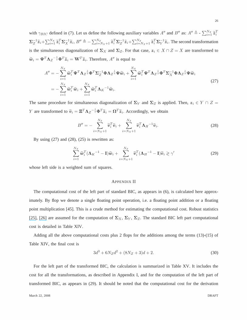
28

significantly reduced computational cost. The computationalgain in flops is defined as the subtraction of

the standard BIC computational cost minus the transformed BIC computational cost. The aforementioned

computational gain, with respect to variousNZ and d values, can be seen in Figure 4. The total

NZ

Com

puta

tiona

lga

inin

flops

d=48d=72d=96

1 1.5 2 2.5 3 3.5 4×104

0

1

2

3

4

5

6

7

8

Fig. 4. The computational gain in flops for severalNZ andd values.

computational cost gain if the speaker utterance duration estimation is used in conjunction with the

transformed BIC rather than the standard BIC with no speakerutterance duration estimation, equals

1 − ur

30d3+(4NZ+4)d2+(7NZ+9)d+53d3+6NZd2+(8NZ+3)d+2 %.

REFERENCES

[1] H. G. Kim and T. Sikora “Comparison of MPEG-7 audio spectrum projection features and MFCC applied to speaker

recognition, sound classification and audio segmentation”, in Proc.2004 IEEE Int. Conf. Acoustics, Speech, and Signal

Processing, vol. 5, pp. 925-928, Montreal, Canada, May 2004.

[2] The Segmentation Task: Find the Story Boundaries, http://www.nist.gov/speech/tests/tdt/tdt99/presentations/NIST

segmentation/index.htm

[3] NIST Rich Transcription Evaluation, http://www.nist.gov/speech/tests/rt/

[4] T. Wu, L. Lu, K. Chen, and H. Zhang, “UBM-based real-time speaker segmentation for broadcasting news”, in Proc.2003

IEEE Int. Conf. Acoustics, Speech, and Signal Processing, vol. 2, pp. 193-196, Hong Kong, April, 2003.

[5] S. Know and S. Narayanan, “Unsupervised speaker indexing using generic models”,IEEE Trans. Audio, Speech, and

Language Processing, vol. 13, no. 5, pp. 1004-1013, September 2005.

[6] M. Collet, D. Charlet, and F. Bimbot, “A correlation metric for speakertracking using anchor models”, in Proc.2005 IEEE

Int. Conf. Acoustics, Speech, and Signal Processing, vol. 1, pp. 713-716, Philadelphia, USA, March 2005.

[7] A. Tritschler and R. Gopinath, “Improved speaker segmentation and segments clustering using the Bayesian information

criterion”, in Proc.6th European Conf. Speech Communication and Techology, pp. 679-682, Budapest, Hungary, September

1999.

March 22, 2008 DRAFT

29

[8] H. Kim, D. Elter, and T. Sikora, “Hybrid speaker-based segmentation system using model-level clustering,” in Proc.2005

IEEE Int. Conf. Acoustics, Speech, and Signal Processing, vol. I, pp. 745-748, Philadelphia, USA, March 2005.

[9] S. Meignier, D. Moraru, C. Fredouille, J. F. Bonastre, and L. Besacier, “Step-by-step and integrated approaches in broadcast

news speaker diarization”,Computer Speech and Language, vol. 20, no. 2-3, pp. 303-330, April-July 2006.

[10] J. A. Arias, J. Pinquier, and R. Andre-Obrecht, “Evaluation of classification techniques for audio indexing”,in Proc.13th

European Signal Processing. Conf., Antalya, Turkey, September 2005.

[11] S. Know and S. Narayanan, “Speaker change detection using a new weighted distance measure,” in Proc.Int. Conf. Spoken

Language, vol. 4, pp. 2537-2540, Colorado, USA, September 2002.

[12] P. Delacourt and C. J. Wellekens, “DISTBIC: A speaker-based segmentation for audio data indexing”,Speech Communi-

cation, vol. 32, pp. 111-126, September 2000.

[13] L. Lu and H. Zhang, “Unsupervised speaker segmentation and tracking in real-time audio content analysis”,Multimedia

Systems, vol. 10, no. 4, pp. 332-343, April 2005.

[14] H. Harb and L. Chen, “Audio-based description and structuring of videos”, Int. J. Digital Libraries, vol. 6, no. 1, pp.

70-81, February 2006.

[15] B. Zhou and J. H. L. Hansen, “Efficient audio stream segmentation via the combinedT 2 statistic and the Bayesian

information criterion”,IEEE Trans. Audio, Speech, and Language Processing, vol. 13, no. 4, pp. 467-474, July 2005.

[16] J. H. L. Hansen, R. Huang, B. Zhou, M. Seadle, J. R. Deller, A.R. Gurijala, M. Kurimo, and P. Angkititrakul, “SpeechFind:

Advances in spoken document retrieval for a national gallery of the spoken word”, IEEE Trans. Audio, Speech, and

Language Processing, vol. 13, no 5, pp. 712- 730, September 2005.

[17] M. Cettolo and M. Vescovi, “Efficient audio segmentation algorithms based on the BIC”, in Proc.2003 IEEE Int. Conf.

Acoustics, Speech, and Signal Processing, vol. 6, pp. 537-540, Hong Kong, April 2003.

[18] J. Ajmera, I. McCowan, and H. Bourlard, “Robust speaker change detection”,IEEE Signal Processing Letters, vol. 11,

no. 8, pp. 649-651, August 2004.

[19] D. A. Reynolds and P. Torres-Carrasquillo, “Approaches andapplications of audio diarization”, in Proc.2005 IEEE Int.

Conf. Acoustics, Speech, and signal Processing,vol. 5, pp. 953-956, Philadelphia, USA, March 2005.

[20] C. H. Wu, Y. H. Chiu, C. J. Shia, and C. Y. Lin, “Automatic segmentation and identification of mixed-language speech

using delta-BIC and LSA-based GMMs”,IEEE Trans. Audio, Speech, and Language Processing, vol. 14, no. 1, pp. 266-

276, January 2006.

[21] M. Kotti, L. G. P. M. Martins, E. Benetos, J. S. Cardoso, and C. Kotropoulos, “Automatic speaker segmentation using

multiple features and distance measures: A comparison of three approaches”, in Proc.2006 IEEE Int. Conf. Multimedia

and Expo, pp. 1101-1104, Toronto, Canada, July 2006.

[22] C. H. Wu and C. H. Hsieh, “Multiple change-point audio segmentationand classification using an MDL-based Gaussian

model”, IEEE Trans. Audio, Speech, and Language Processing, vol. 14, no. 2, pp. 647- 657, March 2006.

[23] S. Cheng and H. Wang, “Metric SEQDAC: A hybrid approach for audio segmentation”, in Proc.8th Int. Conf. Spoken

Language Processing, Jeju, Korea, October 2004.

[24] F. Van der Heijden, R. P. W. Duin, D. de Ridder, and D. M. J. Tax,Classification, Parameter Estimation and State

Estimation: An Engineering Approach Using MATLAB, London, UK: Wiley, 2004.

March 22, 2008 DRAFT

30

[25] N. A. Campbell, “Robust procedures in multivariate analysis I: Robust covariance estimation”,Applied Statistics, vol. 29,

no. 3, pp. 231-237, 1980.

[26] G. A. F. Seber,Multivariate Observations, N.Y.: John Wiley and Sons, 1994.

[27] S. Tadjudin and D. A. Landgrebe, “Covariance estimation with limited training samples,”,IEEE Trans. Geoscience and

Remote Sensing, pp. 2113-2118, vol. 37, no. 4, July 1999.

[28] J. S. Garofolo, “DARPA TIMIT Acoustic-Phonetic Continuous Speech Corpus”, Linguistic Data Consortium, Philadelphia,

1993.

[29] R. D. Reiss and M. Thomas,Statistical Analysis of Extreme Values, Basel : Birkhauser Verlag, 1997.

[30] M. Kotti, E. Benetos, C. Kotropoulos, and I. Pitas, “A neural network approach to audio-assisted movie dialogue detection”,

Neurocomputing, Special Issue: Advances in Neural Networks for Speech and Audio Processing, vol. 71, no. 1-3, pp. 157-

166, December 2007.

[31] J. L. Folks and R. S. Chhikara, “The inverse Gaussian distributionand its statistical application - A review”,J. R. Statist.

Soc. B, vol. 40, pp. 263-289, 1978.

[32] N. L. Johnson, S. Kotz, and S. Balakrishnan,Continuous Univariate Distributions, Volume 1, N.Y.: Wiley, 1994.

[33] S. I. Boyarchenko and S. Z. Levendorskii, “Perpetual american processes under Levi processes”,SIAM J. Control Optim.,

vol. 40, no. 6, pp. 1514-1516, June 2001.

[34] M. C. K. Tweedie, “Statistical properties of inverse Gaussian distributions I”, Annals of Mathematical Statistics, vol. 28,

no. 2, pp. 362-377, June 1957.

[35] X. D. Huang, A. Acero, and H. -S. Hon,Spoken Language Processing: A Guide to Theory, Algorithm, and System

Development, Upper River Saddle: Pearson Education - Prentice Hall, 2001.

[36] R. Kohavi and G. H. John, “Wrappers for feature subset selection”, Artificial Intelligence, pp. 273-324, vol. 97, no. 1-2,

December 1997.

[37] G. Almpanidis and C. Kotropoulos, “Phonemic segmentation using thegeneralised Gamma distribution and small sample

Bayesian information criterion,”Speech Communication, vol. 50, no. 1, pp. 38-55, January 2008.

[38] M. Kotti, V. Moschou, and C. Kotropoulos, “Speaker segmentationand clustering”,Signal Processing, vol. 88, no. 5, pp.

1091-1124, May 2008.

[39] J. J. Barnette and J. E. McLean, “The Tukey honestly significantdifference procedure and its control of the type I error-rate”,

in Proc.Annual meeting Mid-South Educational Research Association, New Orleans, LA, 1998.

[40] C. Barras, X. Zhu, S. Meignier, and J. L. Gauvain, “Multistage speaker diarization of broadcast news”,IEEE Trans. Audio,

Speech, and Language Processing, pp. 1505-1512, vol. 14, no. 5, September 2006.

[41] J. Fiscus, “1997 English Broadcast News Speech (HUB4)”, Linguistic Data Consortium, Philadelphia, 1998.

[42] D. Graff, J. Fiscus, and J. Garofolo, “1997 HUB4 English Evaluation Speech and Transcripts”, Linguistic Data Consortium,

Philadelphia, 2002.

[43] R. R. Korfhage,Information Storage and Retrieval, USA: Wiley and Sons, 1997.

[44] S. Strassel, C. Walker, and H. Lee, “RT-03 MDE Training Data Speech”, Linguistic Data Consortium, Philadelphia, 2004.

[45] G. H. Golub and C. F. Van Loan,Matrix Computations. 3rd Ed., Baltimore, MD, USA: The Johns Hopkins Univ. Press,

1996.

March 22, 2008 DRAFT