continuous reservoir simulation model updating and - CORE

CONTINUOUS RESERVOIR SIMULATION MODEL UPDATING AND

FORECASTING USING A MARKOV CHAIN MONTE CARLO METHOD

A Thesis

by

Chang Liu

Submitted to the Office of Graduate Studies of Texas A&M University

in partial fulfillment of the requirements for the degree of

MASTER OF SCIENCE

December 2008

Major Subject: Petroleum Engineering

CONTINUOUS RESERVOIR SIMULATION MODEL UPDATING AND

FORECASTING USING A MARKOV CHAIN MONTE CARLO METHOD

A Thesis

by

Chang Liu

Submitted to the Office of Graduate Studies of Texas A&M University

in partial fulfillment of the requirements for the degree of

MASTER OF SCIENCE

Approved by: Chair of Committee, Duane A. McVay Committee Members, Akhil Datta-Gupta Jianhua Huang Head of Department, Stephen A. Holditch

December 2008

Major Subject: Petroleum Engineering

iii

ABSTRACT

Continuous Reservoir Simulation Model Updating and Forecasting Using a Markov

Chain Monte Carlo Method.

(December 2008)

Chang Liu, B.A., Peking University, China

Chair of Advisory Committee: Dr. Duane A. McVay

Currently, effective reservoir management systems play a very important part in

exploiting reservoirs. Fully exploiting all the possible events for a petroleum reservoir is a

challenge because of the infinite combinations of reservoir parameters. There is much

unknown about the underlying reservoir model, which has many uncertain parameters.

MCMC (Markov Chain Monte Carlo) is a more statistically rigorous sampling method,

with a stronger theoretical base than other methods. The performance of the MCMC

method on a high dimensional problem is a timely topic in the statistics field.

This thesis suggests a way to quantify uncertainty for high dimensional problems by

using the MCMC sampling process under the Bayesian frame. Based on the improved

method, this thesis reports a new approach in the use of the continuous MCMC method

for automatic history matching. The assimilation of the data in a continuous process is

done sequentially rather than simultaneously. In addition, by doing a continuous process,

the MCMC method becomes more applicable for the industry. Long periods of time to

run just one realization will no longer be a big problem during the sampling process. In

iv

addition, newly observed data will be considered once it is available, leading to a better

estimate.

The PUNQ-S3 reservoir model is used to test two methods in this thesis. The methods are:

STATIC (traditional) SIMULATION PROCESS and CONTINUOUS SIMULATION

PROCESS. The continuous process provides continuously updated probabilistic forecasts

of well and reservoir performance, accessible at any time. It can be used to optimize

long-term reservoir performance at field scale.

v

DEDICATION

To all my friends who have always stood by me

vi

ACKNOWLEDGEMENTS

I would like to thank my parents for their continuing support of my pursuit of knowledge.

vii

TABLE OF CONTENTS

Page ABSTRACT................................................................................................................. iii

DEDICATION...............................................................................................................v

ACKNOWLEDGEMENTS..........................................................................................vi

TABLE OF CONTENTS............................................................................................ vii

LIST OF TABLES ........................................................................................................ix

LIST OF FIGURES .......................................................................................................x

INTRODUCTION .........................................................................................................1

BACKGROUND ...........................................................................................................3

Uncertainty Quantification Techniques....................................................................3 Gradient Methods ............................................................................................................4 MCMC Method................................................................................................................4 Real-Time Data and Ensemble Kalman Filter ...........................................................6

Justification for Continuous Approach.....................................................................8 OBJECTIVE ................................................................................................................10

STATIC SIMULATION PROCESS.............................................................................11

Overview ................................................................................................................11 Parameter Space .....................................................................................................11 Posterior Distribution .............................................................................................12 Metropolis-Hasting MCMC Algorithm..................................................................13 Objective Function .................................................................................................16 Good Mixing and Convergence .............................................................................16 Forecasting .............................................................................................................19

CONTINUOUS SIMULATION PROCESS................................................................22

Overview ................................................................................................................22 Continuous Data and Changed Objective Function ...............................................22 Forecasting .............................................................................................................23

PRIOR MODEL...........................................................................................................25

viii

Page

Overview ................................................................................................................25 Construct the Initial Model ....................................................................................26 Uncertainty Parameters ..........................................................................................37 The Prior Distribution ............................................................................................38

STATIC RESERVOIR STUDY ...................................................................................48

Overview ................................................................................................................48 The Likelihood Function........................................................................................48 The Posterior Distribution......................................................................................50 Parameter Space Search .........................................................................................51 Forecast ..................................................................................................................57 Summary of Results ...............................................................................................66

CONTINUOUS RESERVOIR STUDY ......................................................................67

Overview ................................................................................................................67 The Likelihood Function........................................................................................68 The Posterior Distribution......................................................................................70 Parameter Space Search .........................................................................................71 Forecast ..................................................................................................................74 Calibration of Uncertainty Estimates .....................................................................89 Summary of Results ...............................................................................................97

CONCLUSIONS AND RECOMMENDATIONS ......................................................98

Conclusions ............................................................................................................98 Recommendations for Future Work .......................................................................99

NOMENCLATURE ..................................................................................................100

REFERENCES ..........................................................................................................102

VITA..........................................................................................................................104

ix

LIST OF TABLES

Page

Table 1 - Porosity values at well locations for PUNQ-S3 reservoir .....................35

Table 2 - Average porosity value of each layer for PUNQ-S3 reservoir ..............36

Table 3 - Average permeability value of each layer for PUNQ-S3 reservoir .......37

Table 4 - Porosity distribution factors of initial model .........................................39

Table 5 - Log horizontal permeability distribution factors of initial model..........40

Table 6 - Horizontal permeability distribution factors of initial model ................41

Table 7 - Vertical permeability distribution factors of initial model ....................41

Table 8 - Observed data in static case ...................................................................50

Table 9 - Observed data in the continuous case (each color sequence corresponds to a different data assimilation) .........................................69

x

LIST OF FIGURES

Page

Fig. 1 - Code flow chat .........................................................................................15

Fig. 2 - Objective function vs. models of a MCMC chain in static case ..............19

Fig. 3 - Objective function vs. models of a MCMC chain in continuous case .....23

Fig. 4 - Structure of the PUNQ synthetic reservoir ..............................................27

Fig. 5 - Truth case porosity of Layer 1 .................................................................28





Fig. 10 - Truth case horizontal permeability of Layer 1 .......................................30





Fig. 15 - Truth case vertical permeability of Layer 1 ...........................................33





Fig. 20 - Multiplier regions...................................................................................38

Fig. 21 - Histogram of prior porosity multiplier distribution................................42

Fig. 22 - Histogram of prior permeability multiplier distribution ........................43

xi

Page

Fig. 23 - CDF of prior porosity multiplier ............................................................44

Fig. 24 - CDF of prior permeability multiplier .....................................................45

Fig. 25 - Histogram comparison between high acceptance rate chain and the truth...........................................................................54

Fig. 26 - Histogram comparison between low acceptance

rate chain and the truth...........................................................................55

Fig. 27 - Histogram comparison between proper acceptance rate chain and the truth...........................................................................56

Fig. 28 - Objective function value vs. model number (static case).......................58

Fig. 29 - Mixed well objective function value vs. model number (static case) ....59

Fig. 30 - Histogram of cumulative oil production made by static case ................60

Fig. 31 - CDF of cumulative production by mixed well models in static case.....61

Fig. 32 - Synthetic test forecast compared. A comparison of forecasts from the synthetic static test to published forecast for the PUNQ reservoir .....................................................................................62

Fig. 33 - CDF comparison between prior and posterior (static case). ..................63

Fig. 34 - Posterior permeability assessments (static case). ...................................65

Fig. 35 - Continuous test run number by time. Run number versus point in

reservoir life for the continuous test. .....................................................73

Fig. 36 - Objective function value vs. model number in continuous case ............77

Fig. 37 - Synthetic test forecast using model between 4.5 to 5 years (runs 1-4,500).........................................................................................78

Fig. 38 - Synthetic test forecast using model between 5 to 6 years

(runs 4,501-13,500)................................................................................78

Fig. 39 - Synthetic test forecast using model between 6 to 7 years (runs 13,501-22,500)..............................................................................79


(runs 22,501-31,500)..............................................................................79

xii

Page

Fig. 41 - Synthetic test forecast using model between 7 to 8 years (runs 31,501-40,500)..............................................................................80


(runs 40,501-49,500)..............................................................................80

Fig. 43 - Continuous test forecast CDFs. A comparison of the cumulative distribution functions for various forecasts made during each year (or half year). .........................................................................................81

Fig. 44 - Synthetic test forecast compared. A comparison of forecasts from

the synthetic continuous test to published forecast for the PUNQ reservoir .....................................................................................82

Fig. 45 - Comparison of objective function value between static case and

continuous case, with 9,000 models made between years 9 and 10. .....83

Fig. 46 - Comparison of forecasts between static case and continuous case, with 9,000 models made between years 9 and 10..................................84

Fig. 47 - Comparison of cumulative production CDFs between static case

and continuous case, with 9,000 models made between years 9 and 10. .......................................................................................85

Fig. 48 - Posterior and prior distribution of permeability assessment

(Continuous case)...................................................................................86

Fig. 49 - Continuous test forecast CDFs. A comparison of the cumulative distribution functions for various forecasts made using two years of samples. ...................................................................88

Fig. 50 - Continuous test forecast CDFs. A comparison of the cumulative

distribution functions for various forecasts made using all the models in previous years........................................................................89

Fig. 51 - Continuous test forecast using model between 4.5 to 5 years

(runs 1-4,500) with enlarged prior distribution. ...................................91

Fig. 52 - Continuous test forecast using model between 5 to 6 years (runs 4,501-13,500) with enlarged prior distribution. ..........................92

Fig. 53 - Continuous test forecast using model between 6 to 7 years

(runs 13,501-22,500) with enlarged prior distribution. ........................92

Fig. 54 - Continuous test forecast using model between 7 to 8 years (runs 22,501-31,500) with enlarged prior distribution. ........................93

xiii

Page

Fig. 55 - Continuous test forecast using model between 8 to 9 years (runs 31,501-40,500) with enlarged prior distribution. ........................93

Fig. 56 - Continuous test forecast using model between 9 to 10 years

(runs 40,501-49,500) with enlarged prior distribution. ........................94

Fig. 57 - Continuous test forecast CDFs with enlarged prior. A comparison of the cumulative distribution functions for various forecast made during each year (or half year)...............................................................95

Fig. 58 - Continuous test forecasts compared. A comparison of forecasts

between the original prior distribution and enlarged prior distribution. ...................................................................................96

1

INTRODUCTION

Determining how to effectively exploit oil and gas reservoirs is a central goal in reservoir

management (Thakur 1996). Today’s competitive economic situation requires

cost-effective production technology to profitability produce marginal petroleum

reservoirs. Reservoir simulation is regarded as a critical tool in modern reservoir

management (Thomas 1986). It enables assessment of reservoir properties and, when a

forecast run is made, an assessment of future production and reserves. These assessments

feed directly into the decision-making process.

Capen (1976) demonstrated thirty years ago that people in the petroleum industry often

significantly underestimate uncertainty in their assessments. In keeping with this

tendency, reservoir simulation engineers traditionally take only limited consideration of

uncertainty and in many cases do not try to quantify it at all. Quantifying uncertainty in

production forecasts is not a trivial undertaking. When quantifying the uncertainties, all

possible outcomes of uncertain events should be considered and assigned probabilities in

order to build up a probability density function of the result of interest, e.g., reserves

(Howard 2005). Expressing results in term so probability

__________ This thesis follows the style of SPE Journal.

2

distributions enables better decision making. However, the decision may be poor if the

uncertainty quantification in a forecast is incomplete, or nonexistent. For this reason it is

necessary to rigorously quantify uncertainty in production forecast.

Unfortunately, fully assessing all the possible events for a petroleum reservoir is a quite

challenging because the reservoir parameter space, the set of all possible combinations of

reservoir parameters, is literally infinite. Recent study, e.g., Floris et al. (2001), has

shown that, even when we explicitly try to quantify uncertainty in simulation studies, we

still tend to underestimate it. Therefore, it is worthwhile to explore reservoir simulation

techniques aimed at better quantifying uncertainty in forecasts.

Because of the time and manpower required to tune each parameter in order to history

match a simulation model, reservoir studies are usually expensive. Traditional simulation

studies are usually done only at discrete points in the life of a reservoir, e.g., when

considering a major investment. As such, smaller reservoir management decisions

typically do not warrant the expense of a simulation study and thus must proceed without

simulation results. As a result, uncalibrated forecasts or no forecasts at all could lead to

sub-optimal operations and significant economic consequences. Clearly, reservoir

management would benefit if a calibrated simulation model was available at any time.

3

BACKGROUND

Uncertainty Quantification Techniques

In the past few years, significant work on developing more rigorous uncertainty

quantification has been presented in the literature. Specifically, in the PUNQ work, which

is probably the most thorough treatment of uncertainty quantification in production

forecasts, several industrial and academic partners used different methods to quantify the

uncertainties. The overall objective of the PUNQ project was to determine whether a

methodology can be developed that propagates the combined reservoir modeling,

reservoir parameter and well observation uncertainties to production forecasting

uncertainty in a formally unbiased way.

In this study, we will try to quantify the uncertainty of the reservoir associate with

observed history data, which is called history matching. The main process of performing

a history matching method includes three steps. First, the reservoir is defined in terms of

a reservoir parameter set describing the geometry and flow properties. Next, the

uncertainty parameters of the reservoir are determined by assigning with probabilistic

distributions. Finally, based on the sampled reservoir model, we compare the data from

the simulator with the actual observed data to minimize the objective function, which is

used in the reservoir simulation process to quantify the difference between simulation

results and observed data. Lots of methods exist for searching reasonable models. I will

describe some of them below.

4

Gradient Methods

Gradient methods are used for minimizing the objective function. The Steepest Descent

Method(Bos 1999), the Coordinate Descent Method, and the Conjugate Gradient Method

are three methods widely used to find the direction of variables. Every one of them uses

an iterative formula that contains the gradient of the objective function to find the

minimum, hence the name "Gradient Methods." The goal of these methods is

optimization, which means the result usually comes out to be just one best reservoir

model that fits observation. The method can be stopped when the maximum number of

iterations is exceeded or the requested accuracy is obtained for the solution.

The limitation of the gradient method is that we are usually concerned with getting a

range of what will happen in the future with associated probabilities. Specifically, the

optimum case may not fit our objective in case when we want to get an uncertainty range

instead of one optimum model. Also, the gradient method only works well for smooth

functions. As the reservoir model is usually complicated, the function we are trying to

optimize is usually not smooth. Using gradient methods can lead to biased optimization.

MCMC Method

The Markov Chain Monte Carlo (MCMC) method has been widely used as a strong tool

to sample from a complicated distribution function, especially when we do not know the

exact form of that function. This method originated in physics as a tool for exploring

equilibrium distributions of interacting molecules. In statistical applications, it is used to

5

generate pseudo-random draws from multidimensional and otherwise intractable

probability distributions via Markov chains. A Markov chain is a sequence of random

variables in which each element depends only on the value of the previous one. In

MCMC simulation, one constructs a Markov chain long enough for the distribution of the

elements to stabilize to a stationary distribution, which is the distribution of interest. By

repeatedly simulating steps of the chain, the method simulates draws from the distribution

of interest.

In reservoir modeling research, MCMC has been applied as a method for exploring

posterior distributions in Bayesian inference. The final distribution is simply generated

from a set of samples, which are reservoir models in our study. First, a randomly sampled

model is built up from a prior distribution. It is also the start point of the Markov chain.

Then, the next model is randomly chosen with some constraints related to the previous

model which is already in the chain. After the chain is run long enough, we are able to use

the models in the chain to generate the posterior distribution. Once the distribution is

generated, it is easy to get the range of uncertain parameters with specific probabilities.

Another related method for generating an unknown distribution is called Genetic

Algorithm (Goldberg 1989), which has a variety of applications. Genetic algorithms

(GAs) are a broad class of optimization algorithms based loosely upon the rules that

govern genetics in nature. In a GA, “generations” of unique reservoir models are created

by mixing parameter values of previously run models in a process known as “breeding.”

Finally, all generations are used to generate a distribution (Holmes et al. 2007).

6

Compared to GAs, MCMC is statistically more rigorous by working under the Bayesian

frame. It can also be considered to be a type of GA because the next model relies on some

properties of the previous one, which can be regarded as its parent in GAs.

Although the Markov Chain Monte Carlo methodology is straightforward, how to

efficiently generate the posterior distribution can be quite challenging. The chain often

converges too slowly in history matching, especially when the parameter space is large. A

two-stage MCMC method (Ma et al. 2006) has been used to solve this particular problem

by enhancing the acceptance rate of the next model. Also, Holden (1998) has suggested

an adaptive MCMC method by using all the previous models which are already in the

chain to generate the next one.

Real-Time Data and Ensemble Kalman Filter

Ensemble Kalman Filter (EnKF) techniques are widely used in both statistical field and

petroleum industry field to utilize all available data in order to make probabilistic

forecasts. The EnKF is a Monte Carlo approach, which is promising with respect to

achieving uncertainty quantification through continuous model updating and reservoir

monitoring (Nævdal et al. 2003; Gu and Oliver 2004; Bianco et al. 2007; Devegowda et

al. 2007). The assimilation of data in EnKF is done sequentially rather than

simultaneously as is done in traditional history matching. By doing so the reservoir

models are always kept up to date.

The EnKF starts with an ensemble of reservoir models conditioned to all available static

7

data, e.g., cores, well logs and structural information (Devegowda et al. 2007). These

geologic models constitute the initial ensemble and represent the variability in the

underlying reservoir properties. As and when data become available, the EnKF updates

each of these model realizations using statistical information derived from the ensemble

of models and model predicted data, specifically the cross-covariance between the data

and the model variables. This step is repeated when more data become available. The

underlying algorithm is computationally efficient because the computation of gradients or

sensitivities is eliminated and the updates depend solely on statistical information.

Consequently, the EnKF generates a suite of plausible model realizations conditioned to

production history and, in theory, should honor prior static or geologic information.

However, due to the inherent noise in any statistical measure that is dependent on the

number of samples or model realizations, the EnKF updates can lead to

geologically-inconsistent realizations for small ensemble sizes. Therefore, while the final

realizations may honor historical production data, the models do not conform to the prior

geologic information (Devegowda et al. 2007). The use of a larger ensemble size may

mitigate some of the difficulties in the implementation of the EnKF, but for field-scale

problems this may be computationally expensive. For very small ensemble sizes, the

individual ensemble members tend to converge to a single realization and progressively

ignore future observations. The literature shows examples of the EnKF applied to field

studies (Devegowda et al. 2007), but many of the problems described above remain

unresolved. Some techniques attempt to improve EnKF performance through better

estimates of the cross-covariance matrix using covariance localization techniques. Others

have used the gradient of an appropriately defined objective function to derive other

8

variants of the EnKF. However, the EnKF is still a topic of active research for history

matching purposes and the technique is evolving to address many of the difficulties in its

implementation.

Justification for Continuous Approach

Because of the limitation of geological information, the reservoir parameter uncertainty

space is usually extremely large, even with a coarse parameterization. Obviously, we

cannot test every possible model by making simulation runs. So, the techniques presented

in the PUNQ study (Bos 1999) attempt to quantify uncertainty with relatively few runs.

Techniques like gradient methods attempt to quantify uncertainty using a few hundred

runs, where MCMC and GA applications typically employ one thousand to several

thousand runs to get a better range of uncertainty. Even with MCMC techniques, however,

there are practical limitations. This is because each of these applications has been treated

as a one-time study (fixed period of history data and fixed prediction period). When we

do a one-time study, it has a time limitation issue. We cannot explore the uncertainty

parameter space in a limited time before new available data come out. The problem

becomes more severe for real world simulation models, as it takes hours or even days to

run simulations with complicated reservoir models on powerful servers. If we can

incorporate new data into simulation runs as soon as possible, and the program can run

continuously through the whole span of a reservoir’s life, then our parameter space would

be better explored. Even with large simulation models this offers the potential to make

tens of thousands of simulation runs over the life of the reservoir. These thousands of

runs should yield a more thorough exploration of the parameter space and better

9

probabilistic forecasts. Holmes et al. (2007) demonstrates a continuous updating process

on both PUNQ synthetic reservoir and also a live field test. The production forecast of his

study on PUNQ reservoir does bracket the truth case and also shows a similar uncertainty

range compared to other studies published before (Bos 1999). But unfortunately, the

sampling methodology used in his study is not statistically rigorous compared to MCMC

sampling method. Thus, it would be useful to investigate a statistically rigorous method

which could also cooperate with history data continuously.

10

OBJECTIVE

Based on traditional MCMC, develop an improved continuous MCMC simulation case,

which is more statistically rigorous, by incorporating the data frequently in a continuous

history matching process to evaluate its practicality and effectiveness in generating

probabilistic forecasts. The built-up process will be tested on the PUNQ synthetic

reservoir.

By achieving this objective, I will first implement the traditional MCMC history

matching method on PUNQ as a one-time study. Then, in order to evaluate the

continuous method, I will break up the history data into several parts and add them

sequentially into the history matching process. It is a scenario which imitates the live

field case that we should incorporate with new observed data when it becomes available.

11

STATIC SIMULATION PROCESS

Overview

History matching and generating probabilistic forecasts with the MCMC method requires

the combination of several components. First, the reservoir uncertain parameters and their

associated uncertainties must be determined. Second, as uncertainty in future reservoir

performance is usually evaluated from the simulated performance of a set of reservoir

models, a method of sampling the parameter space and generating reservoir models is

needed. In turn this requires code to automatically run the simulations and read the

production forecast of each single sample. The Markov Chain Monte Carlo Monte

method (MCMC) is applied here to explore the uncertainty parameter space. Finally, the

results of individual runs are combined into probabilistic forecasts. Below, I will describe

the details of each of these components.

Parameter Space

Before doing any simulations, it is necessary to first determine which uncertain

parameters should be considered. In general this is a manual process and relies on the

ability of the reservoir engineer to make assessments based on the available data (Holmes

et al. 2007). In the PUNQ-S3 model simulated here, the parameters considered are

porosity and permeability. Once we identify the parameters of interest, we assign the

prior distributions (usually continuous) to quantitatively represent the uncertainty in these

parameters. The type of distribution that would be appropriate is usually based on

12

reservoir characterization data. In our study of the PUNQ-S3 model, we assume that

permeability adheres to log-normal distribution. Porosity adheres to normal distribution.

This process for identifying uncertain parameters and assigning prior distributions is

fairly consistent with what is traditionally done when assessing input uncertainty in a

simulation study.

Posterior Distribution

The posterior distribution is the refined distribution considering observed data from our

prior distribution. It represents the whole uncertainty with all possible realizations. In this

study, a posterior probability function is built under the Bayesian frame:

( ) ( ) ( )mPmdPdmP obsobs ∝ …………………………………………………………………... (1)

where obsd represents the observed dynamic data from the real field and m represents

the uncertain parameters. ( )mP represents the prior probability distribution of uncertain

parameters determined before. ( )mdP obs is the likelihood function related to our

observed data and ( )obsdmP is our posterior distribution. In particular, if we assume that

the prior model and the data errors follow a Gaussian distribution, then our posterior

distribution ( )obsdmP becomes the following form (Howard 2005):

( ) ( ) ( ) ( )[ ] ( )[ ]⎭⎬⎫

⎩⎨⎧

⎟⎠⎞

⎜⎝⎛ −−−+−−−∝ −−

obsDT

obsmT

obs dmgCdmgmCmdmP 11

21

21exp μμ …. (2)

where ( )mg is the simulated reservoir response, such as water cut, corresponding to the

13

proposed m . mC is the parameter covariance and DC is the data covariance. A more

detailed posterior distribution will be described later in the static case and continuous

case study.

The posterior distribution is typically defined on a high-dimensional parameter space and

often has multiple modes. The Metropolis-Hasting MCMC approach is often applied

(Hastings 1970) to sample from this complicated posterior distribution. The main

objective of the MCMC method is to construct a Markov chain whose stationary

distribution matches the posterior distribution.

Metropolis-Hasting MCMC Algorithm

Metropolis-Hasting MCMC method is used to sample models from our posterior

distribution. Assume we want to sample from the distribution ( )mπ , the posterior

distribution in our study (Hastings 1970).

14

Step 1. At state nm generate m from a specified proposal distribution ( )nmmq

Step 2. Accept m as a sample with the probability

( ) ( ) ( )( ) ( )⎟

⎟⎠

⎞⎜⎜⎝

⎛=

nn

nn mmmq

mmmqmmR

ππ

,1min,

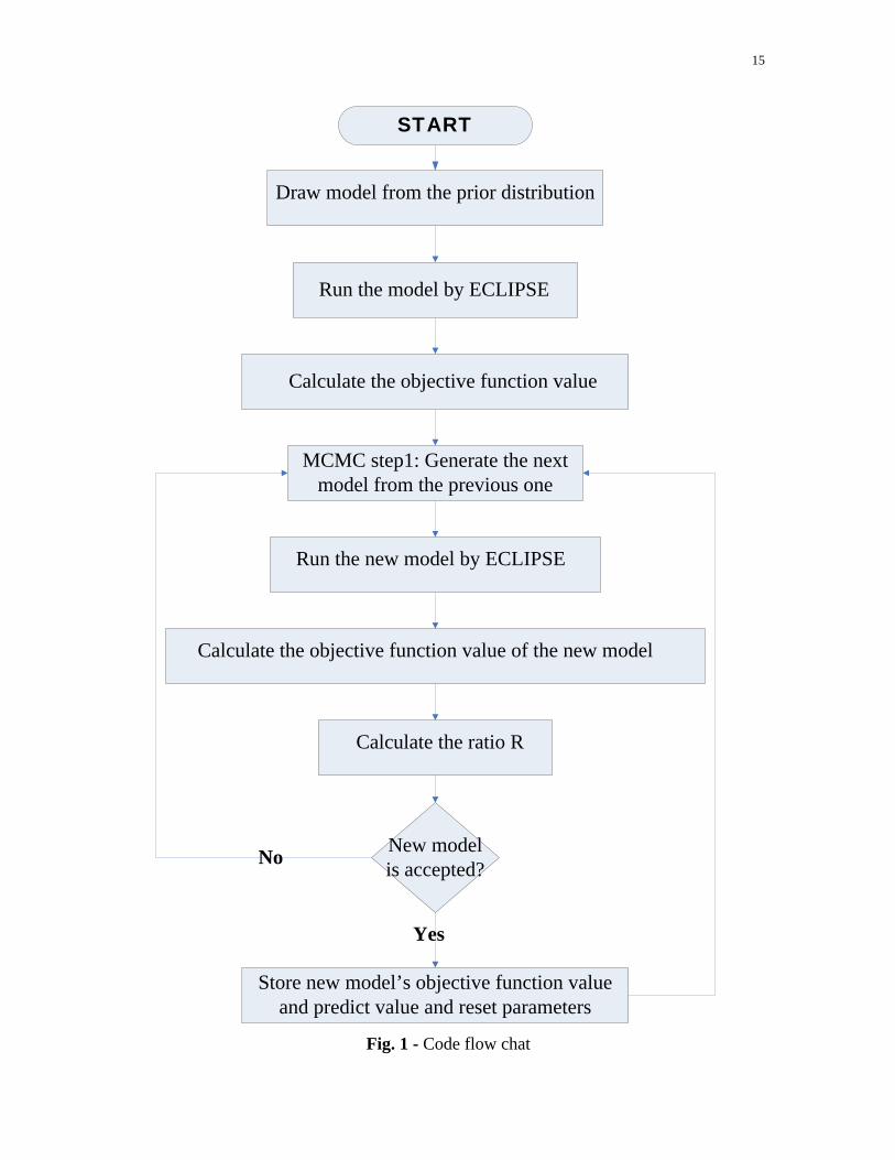
In order for the MCMC process to be practical, simulation runs must run automatically

without human interaction. In this study, a commercial simulator, Eclipse, was used. I did

not have access to the source code, which required the creation of a “wrapper” around the

simulator. This entailed writing additional code to create a file for each run, submit it to

the simulator and read the results. This process obviously could be streamlined by

working directly with the simulator source code. The code flow chart is listed below (Fig.

1):

15

START

Draw model from the prior distribution

Run the model by ECLIPSE

Calculate the objective function value

MCMC step1: Generate the next model from the previous one

Run the new model by ECLIPSE

Calculate the objective function value of the new model

Calculate the ratio R

New model is accepted?

Store new model’s objective function value and predict value and reset parameters

No

Yes

Fig. 1 - Code flow chat

16

Objective Function

An objective function is used to quantitatively evaluate how well an individual model

reproduces the observed data from the field. This term is defined as a part of the posterior

distribution function as

( ) ( ) ( ) ( )[ ] ( )[ ]obsDT

obsmT dmgCdmgmCmmO −−+−−= −− 11 μμ ……………………… (3)

In Eq. 3, ( ) ( )μμ −− − mCm mT 1 is called the prior term and

( )[ ] ( )[ ]obsDT

obs dmgCdmg −− −1 is called the likelihood term. As a result, our objective

function is a combination of prior information and observed information. This is a

consequence of the posterior distribution construction under the Bayesian frame. Also,

we can tell from the posterior distribution expression (Eq.2) that when the value of a

model’s objective function goes down, our posterior distribution value goes up. This

results in a higher possibility model in our posterior distribution. The acceptance ratio R

is defined as the ratio of the posterior values between the new model and the previous

model. The new model with a smaller objective function would have a higher possibility

to be accepted.

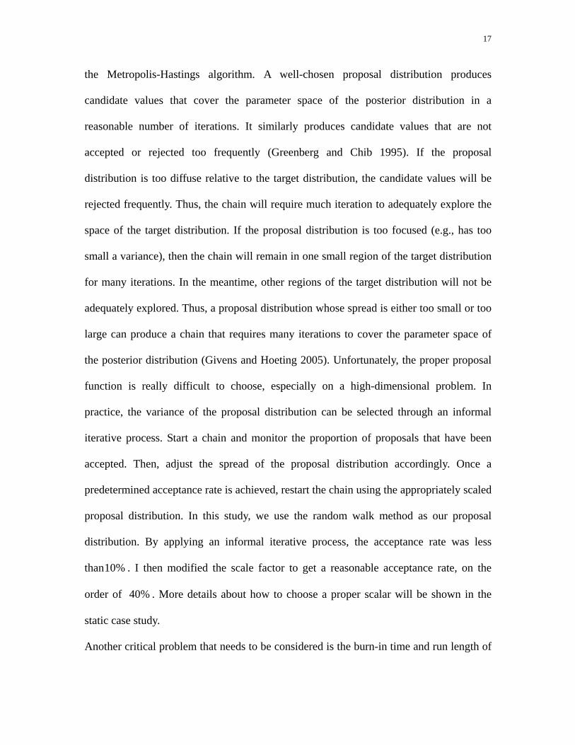
Good Mixing and Convergence

The most important influence during the MCMC sampling process is how to choose the

proposal distribution. Good proposal distributions can greatly enhance the performance of

17

the Metropolis-Hastings algorithm. A well-chosen proposal distribution produces

candidate values that cover the parameter space of the posterior distribution in a

reasonable number of iterations. It similarly produces candidate values that are not

accepted or rejected too frequently (Greenberg and Chib 1995). If the proposal

distribution is too diffuse relative to the target distribution, the candidate values will be

rejected frequently. Thus, the chain will require much iteration to adequately explore the

space of the target distribution. If the proposal distribution is too focused (e.g., has too

small a variance), then the chain will remain in one small region of the target distribution

for many iterations. In the meantime, other regions of the target distribution will not be

adequately explored. Thus, a proposal distribution whose spread is either too small or too

large can produce a chain that requires many iterations to cover the parameter space of

the posterior distribution (Givens and Hoeting 2005). Unfortunately, the proper proposal

function is really difficult to choose, especially on a high-dimensional problem. In

practice, the variance of the proposal distribution can be selected through an informal

iterative process. Start a chain and monitor the proportion of proposals that have been

accepted. Then, adjust the spread of the proposal distribution accordingly. Once a

predetermined acceptance rate is achieved, restart the chain using the appropriately scaled

proposal distribution. In this study, we use the random walk method as our proposal

distribution. By applying an informal iterative process, the acceptance rate was less

than %10 . I then modified the scale factor to get a reasonable acceptance rate, on the

order of %40 . More details about how to choose a proper scalar will be shown in the

static case study.

Another critical problem that needs to be considered is the burn-in time and run length of

18

the chain. With a generated MCMC chain, the iterations may not be enough for the

correct marginal distribution and the dependence on the chain starting point may remain

strong. To reduce the severity of this problem, the early group of elements of the chain is

typically discarded as a burn-in period. The determination of an appropriate burn-in

period and run length is still an active area of research. A commonly used approach is

presented by Gelman and Rubin (1992) but there is potential difficulty with their

approach. For example, selecting suitable starting values in cases of multimodal posterior

distribution may be difficult. Using multiple MCMC chains will not work if all of chains

become stuck in the same sub-region or mode. In our study, we simply cut off the first

group of models, whose objective function’s value is significantly high and use the rest of

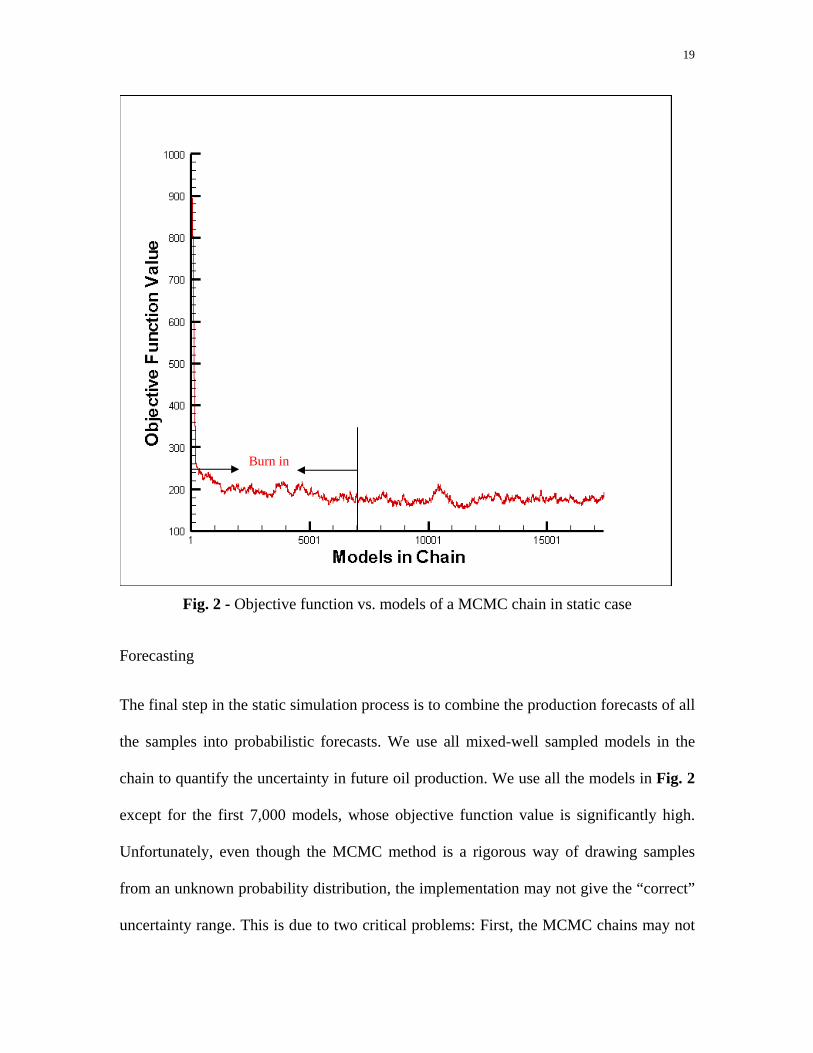
the models to generate our posterior distribution. Fig. 2 shows an objective function

curve in my study, where the first 7,000 models that have high values are considered as

the burn-in period.

19

Fig. 2 - Objective function vs. models of a MCMC chain in static case

Forecasting

The final step in the static simulation process is to combine the production forecasts of all

the samples into probabilistic forecasts. We use all mixed-well sampled models in the

chain to quantify the uncertainty in future oil production. We use all the models in Fig. 2

except for the first 7,000 models, whose objective function value is significantly high.

Unfortunately, even though the MCMC method is a rigorous way of drawing samples

from an unknown probability distribution, the implementation may not give the “correct”

uncertainty range. This is due to two critical problems: First, the MCMC chains may not

Burn in

20

be long enough to fully explore the parameter space or to achieve convergence. This

problem becomes even more difficult to handle as there are too many uncertain

parameters considered in the updating process. Secondly, the choice of the history match

quality definition (i.e., likelihood function) is also crucial. Barker et al. (2001) provide an

alternative approach to create probabilistic forecasts which they claim is statistically

rigorous. Barker models uncertainty using the exponential likelihood function as

⎥⎥⎦

⎤

⎢⎢⎣

⎡⎥⎦

⎤⎢⎣

⎡ −−×= ∑

2

121exp

n

i

obsi

calci yycLσ

…………………………………………………. (4)

Eq. 4 requires that the production data are independent measurements with normally

distributed error, as stated in the paper. Unfortunately, the authors neither reference nor

provide a derivation of this formula. However, Eq. 4 appears to be an adaptation of the

likelihood function for normal distributions, given by Vose (2000) as:

( ) ( )⎥⎦

⎤⎢⎣

⎡ −−⎟⎟

⎠

⎞⎜⎜⎝

⎛= ∑

=

n

i

i

nxL

12

2

2 2exp

21,

σμ

πσσμ ………………………………………… (5)

where ix is the observation from an independent experiment. The major problem with

adapting this formula for use in production forecasts is the assumption of independent

measurements with normally distributed error. In production forecasts the same

observation (such as the pressure in a given well) is made at multiple points in time.

Obviously, the pressure in a well is not completely independent from the pressure at an

21

earlier or later point in time. When dependant data points such as these are used in the

likelihood function, the assumption of independence is violated and the statistical validity

of the approach is called into question. Without any guidance from the authors in the

form of a derivation or reference, this issue cannot be reconciled. In our study, we simply

consider that the observed data are independent of each other. Thus, we use Eq.4 as our

likelihood function, in line with previous researchers.

22

CONTINUOUS SIMULATION PROCESS

Overview

Conducting simulation in the continuous manner is similar to the static case with the

exception of changes made to the objective function. The same initial model is used in the

continuous case. The parameter space is also set to be the same as the static case, in order

to do reasonable comparisons. On the other hand, as we are doing the continuous history

matching process, new data comes from the real field and is added to the objective

function. The updated objective function is then involved in subsequent simulation runs.

Finally, the results of individual runs are combined into probabilistic forecasts.

Continuous Data and Changed Objective Function

At various points in time during the continuous simulation process, new data from the

field become available. It is advantageous to include new data in the process as quickly as

possible, as it is generally assumed that more information from the field leads to better

forecasts and assessments of uncertainty. As more data are added, Eq. 4 will include

more observed data points and simulation data points. As a result, the observed data

misfit term in our objective function will increase. Even though the way changing the

objective function is not statistically rigorous, our objective here is to investigate the

impact of the violation by comparing the forecast results with other researchers. Fig. 3

shows the change of the objective function curve when carrying out the continuous

23

process in my study.

Fig. 3 - Objective function vs. models of a MCMC chain in continuous case

Once the new observed data are incorporated, the current last model in the chain should

be recalculated with a revised objective function. This leads to a bigger objective function

and causes a shift of our objective function curve shown in Fig. 3. New data come in at

model number points 4,500; 13,500; 22,500; 31,500; and 40,500.

Forecasting

Combining the results of the simulation runs into probabilistic forecasts in the continuous

New data added points

24

simulation process is much similar to the static case. In contrast, the continuous case

forecasting can be done at any time by using sampled models in previous years. For

example, in this PUNQ-S3 study we divided the history data into six parts. The process

first starts with all the history data before year 4.5. Then, we add to the history data

sequentially at the 5th, 6th, 7th, 8th and 9th years. If we want to forecast the cumulative

16.5-year oil production at the end of the 9th year, we can simply forecast with the models

sampled in the 9th year.

25

PRIOR MODEL

Overview

Before carrying out the static and continuous MCMC tests on the PUNQ-S3 model, we

first built up the initial model and the prior distribution. The two tests use the same prior

distribution during the history matching process. The PUNQ-S3 synthetic reservoir has

been used in probably the most thorough treatment of uncertainty quantification in

production forecasts. Several industrial and academic partners used different methods to

test a number of history matching techniques. The objectives of the PUNQ project were

to research whether or not a methodology can be developed that propagates the combined

reservoir modeling, reservoir parameter and well observation uncertainties into forecast

uncertainty in a formally unbiased way. The true total oil recovery after the simulation

period is 361087.3 Sm× .

The project provides noisy well porosities and permeabilities and noisy synthetic

production history of the first eight years. This history of the reservoir life includes 1 year

of well testing, 3 years of field shut-in and 4 years of actual field production. The

synthetic production data consisted of the Bottom Hole Pressure (BHP), Water Cut (WCT)

and Gas Oil Ratio (GOR) for each of the 6 wells. Also, within the history period, two

wells show a gas breakthrough and one well shows the onset of water breakthrough (Bos

1999).

26

In our methology, instead of using porosity and permeability values directly, the uncertain

parameters used in our study are porosity and permeability multipliers. These multipliers

are applied to permeability and porosity base maps when running the simulation. The

effect is the same as if porosity and permeability values were used directly, but this

approach simplifies the implementation. As a result, the process for building up the initial

distribution generally breaks into three steps:

1. Construct the initial model.

2. Determine uncertain parameters (multipliers).

3. Build up the prior distributions for uncertain parameters.

Construct the Initial Model

The PUNQ-S3 reservoir model is a five-layer, three-phase synthetic reservoir based on an

actual field operated by Elf. By most standards the PUNQ-S3 reservoir is a small model

with just 1,761 active cells. On a modern desktop computer a single simulation run takes

less than a minute, which is advantageous for making a large number of runs. Based on

available information from the truth case, some properties of the reservoir such as PVT

properties, well information, and schedules were generated. These parts are the same as

the truth case in our initial model.

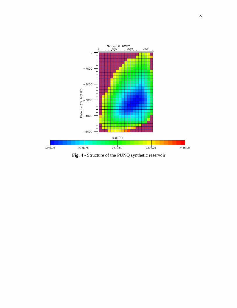
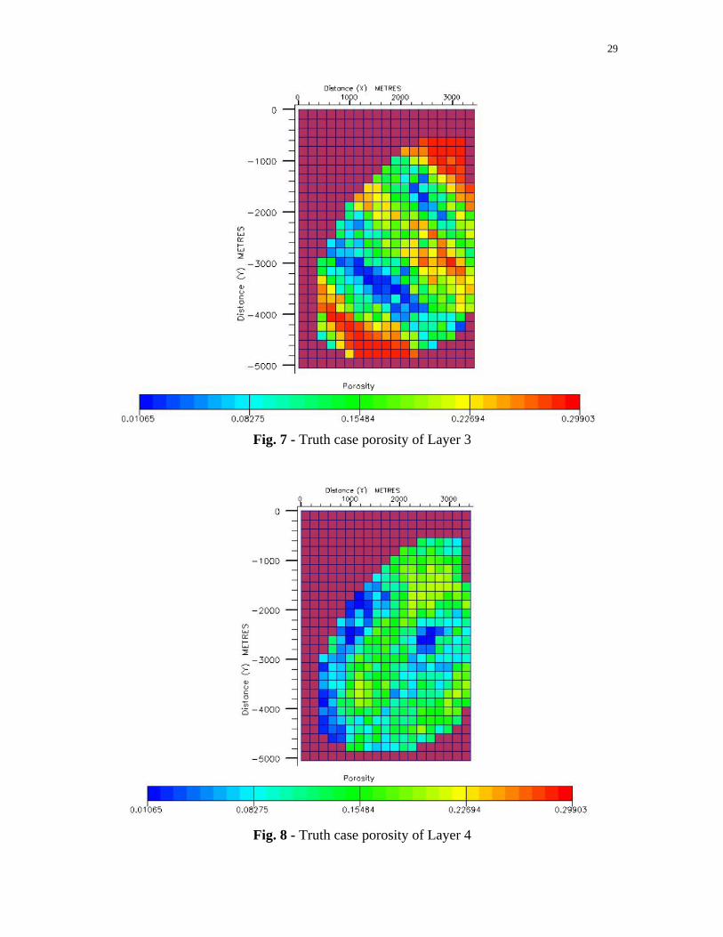
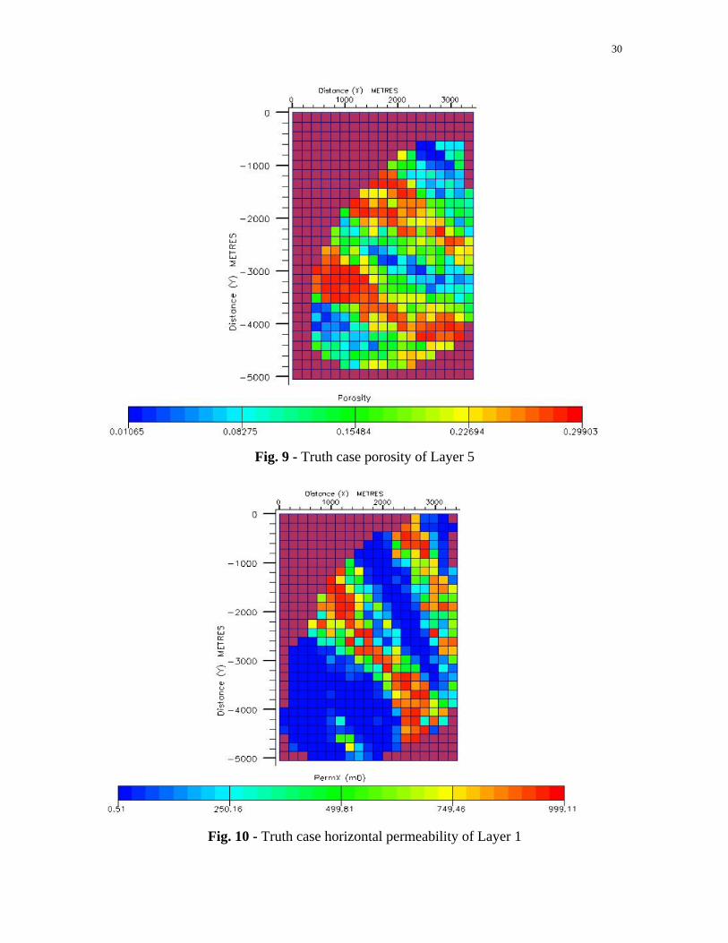
The truth case’s structure map (Fig. 4) and porosity, horizontal and vertical permeability

maps are shown in Figs. 5-20. Since we consider porosity and permeability as our

unknown parameters, the prior model should be set up with a different porosity and

permeability from the truth case for testing purposes.

27

Fig. 4 - Structure of the PUNQ synthetic reservoir

28

Fig. 5 - Truth case porosity of Layer 1


29



30


Fig. 10 - Truth case horizontal permeability of Layer 1

31



32



33

Fig. 15 - Truth case vertical permeability of Layer 1


34



35


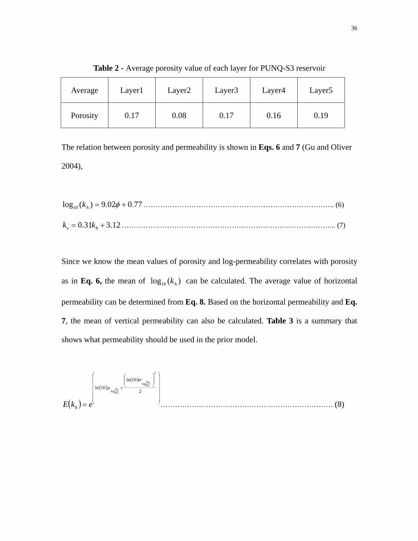
We use the average values of porosity in each layer from well data to generate our prior

porosity. Table 1 (Gu and Oliver 2004) gives the actual porosity values at well locations

and Table 2 shows the average porosity value of each layer.

Table 1 - Porosity values at well locations for PUNQ-S3 reservoir

Well Layer 1 Layer 2 Layer 3 Layer 4 Layer 5

PRO-1 0.0828 0.0616 0.0982 0.1486 0.2445

PRO-4 0.2192 0.0588 0.1114 0.16 0.2137

PRO-5 0.2346 0.0708 0.2115 0.1498 0.0949

PRO-11 0.0828 0.088 0.2434 0.1342 0.151

PRO-12 0.0751 0.1092 0.1048 0.1808 0.2401

PRO-15 0.2783 0.0966 0.1939 0.1995 0.2753

36

Table 2 - Average porosity value of each layer for PUNQ-S3 reservoir

Average Layer1 Layer2 Layer3 Layer4 Layer5

Porosity 0.17 0.08 0.17 0.16 0.19

The relation between porosity and permeability is shown in Eqs. 6 and 7 (Gu and Oliver

2004),

77.002.9)(log10 += φhk …………………………………………………………………….. (6)

12.331.0 += hv kk ……………………………………………………………………………... (7)

Since we know the mean values of porosity and log-permeability correlates with porosity

as in Eq. 6, the mean of )(log10 hk can be calculated. The average value of horizontal

permeability can be determined from Eq. 8. Based on the horizontal permeability and Eq.

7, the mean of vertical permeability can also be calculated. Table 3 is a summary that

shows what permeability should be used in the prior model.

( )

( )( )

⎟⎟⎟⎟⎟⎟

⎠

⎞

⎜⎜⎜⎜⎜⎜

⎝

⎛

⎟⎟⎠

⎞⎜⎜⎝

⎛

+

=

2

10ln10ln

2

10log

10log

hk

hk

ekE h

σ

μ

……………………………………………………………… (8)

37

Table 3 - Average permeability value of each layer for PUNQ-S3 reservoir

Average Layer1 Layer2 Layer3 Layer4 Layer5

Horizontal

permeability 432md 33md 432md 196md 654md

Vertical

permeability 137md 13md 137md 64md 205md

Uncertainty Parameters

Review of the geological description indicates the reservoir is marked by wide

southeast-trending high-quality streaks. As a result, I parameterized the PUNQ-S3 model

using six homogenous regions per layer rather than using rectangular regions. The

defined regions approximate the representation of the shape of these streaks (Fig. 20).

Five layers times 6 regions per layer times three properties (porosity, vertical

permeability and horizontal permeability) yields 90 multipliers that need to be updated

each iteration.

38

Fig. 20 - Multiplier regions

The Prior Distribution

The porosity adheres to a normal distribution and permeability adheres to a log-normal

distribution, which is consistent with practical experience and other research done on the

PUNQ model. Udating the multipliers indirectly is identical with updating permeability

and porosity directly. As shown by Eq. 9, 'φ denotes the constant porosity value in our

base map, φX denotes the porosity multiplier random variable. φ is our final porosity

value in the realization.

'φφ φX= ………………………………………………………………………………………. (9)

39

Eq. 9 shows a linear relationship between porosity multiplier and porosity. So, φX

should follow a normal distribution in order to make our porosity follow a normal

distribution. The mean of our porosity multipliers were chosen to be 1. This is reasonable

because the prior distribution is built up based on our initial model. This means that the

average porosity of each layer should be the most likely realization without any impact by

the observed data. Additionally, the variance and standard deviation of porosity are

shown by Eq. 10 and Eq. 11. Table 4 (Barker et al. 2001), shows the mean and standard

deviation value of porosity in each layer. According to the values in Table 4, the standard

deviation on porosity values should be set to 30% of the mean(an average value). As a

result, the standard deviation of our porosity multiplier should be chosen as 0.3.

( ) )(2'φφφ XVarVar = ……………………………………………………………...………… (10)

( )φφφ Xstdstd ')( = ………………………………………………………………… (11)

Table 4 - Porosity distribution factors of initial model

layer Mean Std Std/Mean 1 0.17 0.06 0.352941 2 0.08 0.02 0.25 3 0.17 0.06 0.352941 4 0.16 0.03 0.1875 5 0.19 0.06 0.315789

The permeability is not as straightforward because we should use a multiplier that applies

to log-normal distribution. This is because our prior permeability follows a log-normal

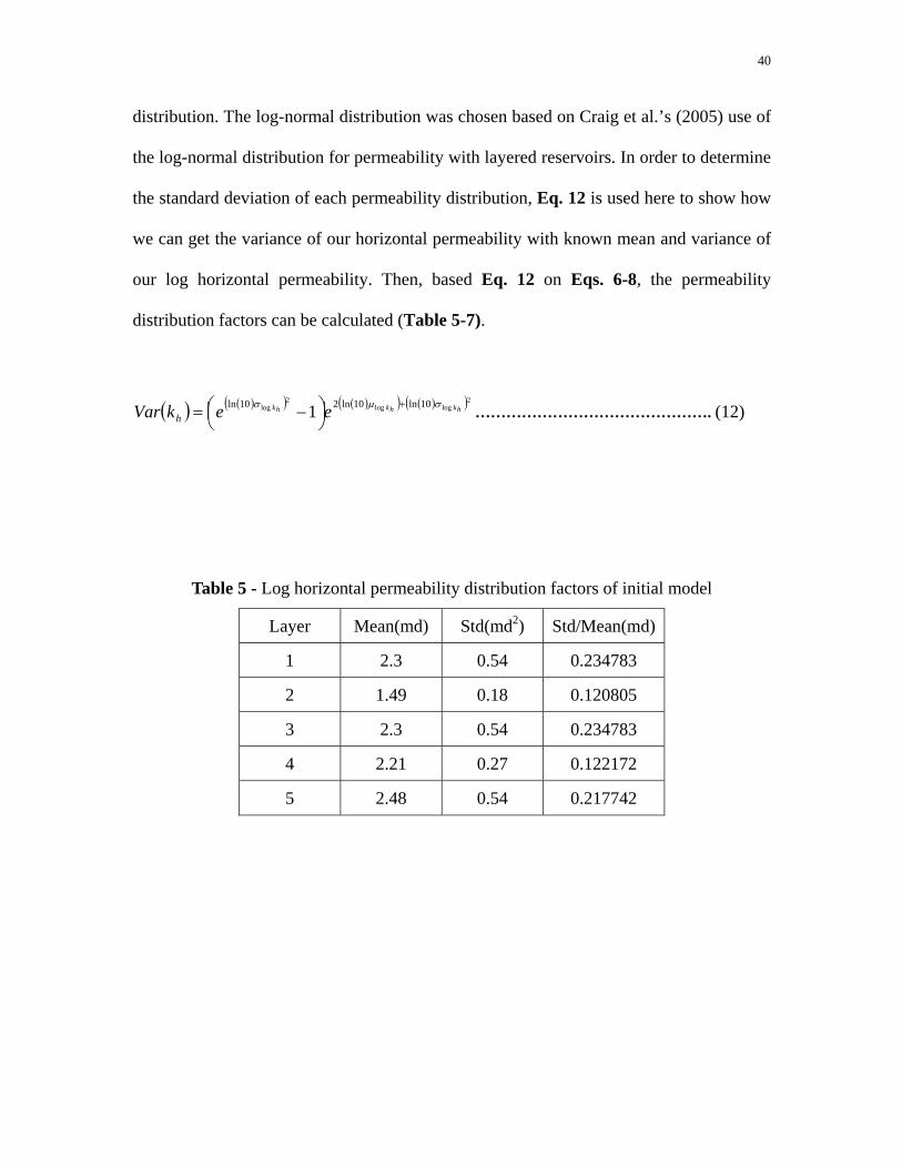
40

distribution. The log-normal distribution was chosen based on Craig et al.’s (2005) use of

the log-normal distribution for permeability with layered reservoirs. In order to determine

the standard deviation of each permeability distribution, Eq. 12 is used here to show how

we can get the variance of our horizontal permeability with known mean and variance of

our log horizontal permeability. Then, based Eq. 12 on Eqs. 6-8, the permeability

distribution factors can be calculated (Table 5-7).

( ) ( )( ) ( )( ) ( )( )2loglog2

log 10ln10ln210ln 1 hkhkhk eekVar hσμσ +⎟

⎠⎞⎜

⎝⎛ −= ………………………………………. (12)

Table 5 - Log horizontal permeability distribution factors of initial model

Layer Mean(md) Std(md2) Std/Mean(md)

1 2.3 0.54 0.234783

2 1.49 0.18 0.120805

3 2.3 0.54 0.234783

4 2.21 0.27 0.122172

5 2.48 0.54 0.217742

41

Table 6 - Horizontal permeability distribution factors of initial model


1 432.232 830.6076 1.921671

2 33.67456 14.57834 0.432918

3 432.232 830.6076 1.921671

4 196.7566 135.1522 0.686901

5 654.2096 1257.176 1.921671

Table 7 - Vertical permeability distribution factors of initial model


1 137.1119 257.4884 1.877943

2 13.55911 4.519284 0.333302

3 137.1119 257.4884 1.877943

4 64.11453 41.89719 0.653474

5 205.925 389.7244 1.892555

Because permeability multiplier applies to a log-normal distribution whose mean is

different from the median, the median of our permeability multiplier is chosen as 1

instead of choosing the mean to be 1. The standard deviation on permeability values was

set to %135 of the mean (an average value of “Std/Mean” from Table 5-7) of initial

permeability, since we only use one prior distribution to characterize the whole reservoir.

Thus, the standard deviation of our log-normal permeability multiplier should be chosen

as 1.35.

So far, all the important factors of our prior distribution have been determined. In order to

prevent extreme and unrealistic values of permeability, the multiplier distribution is

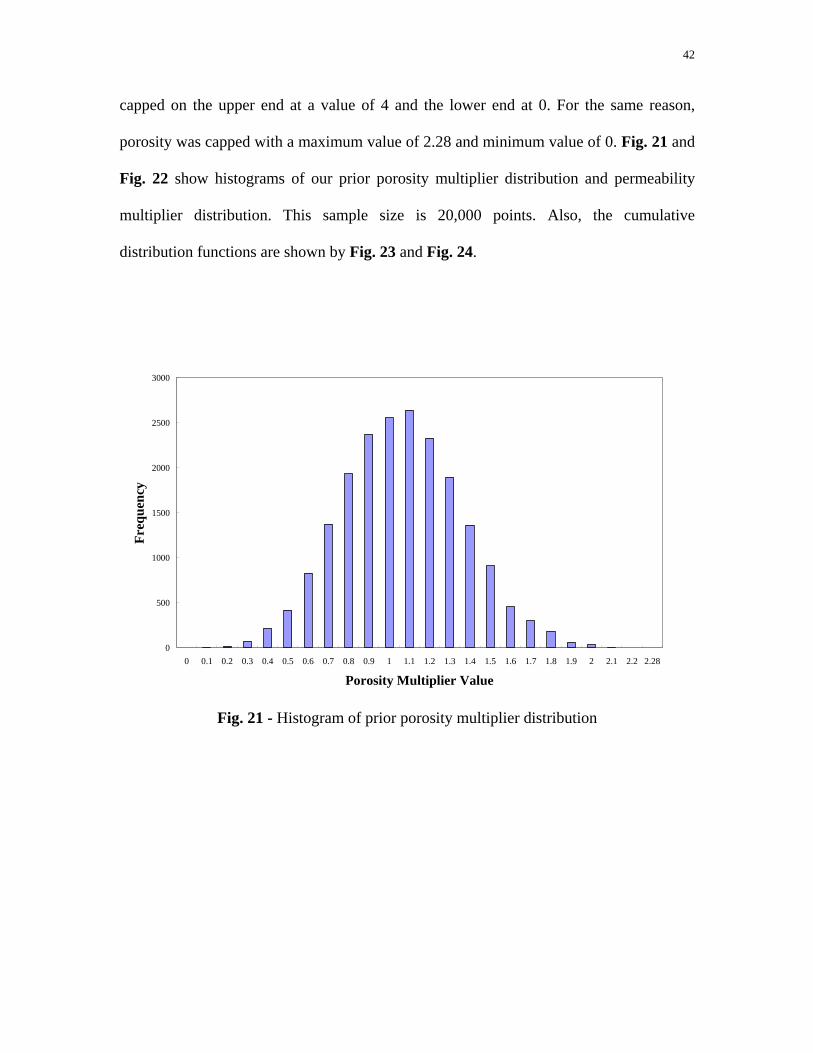
42

capped on the upper end at a value of 4 and the lower end at 0. For the same reason,

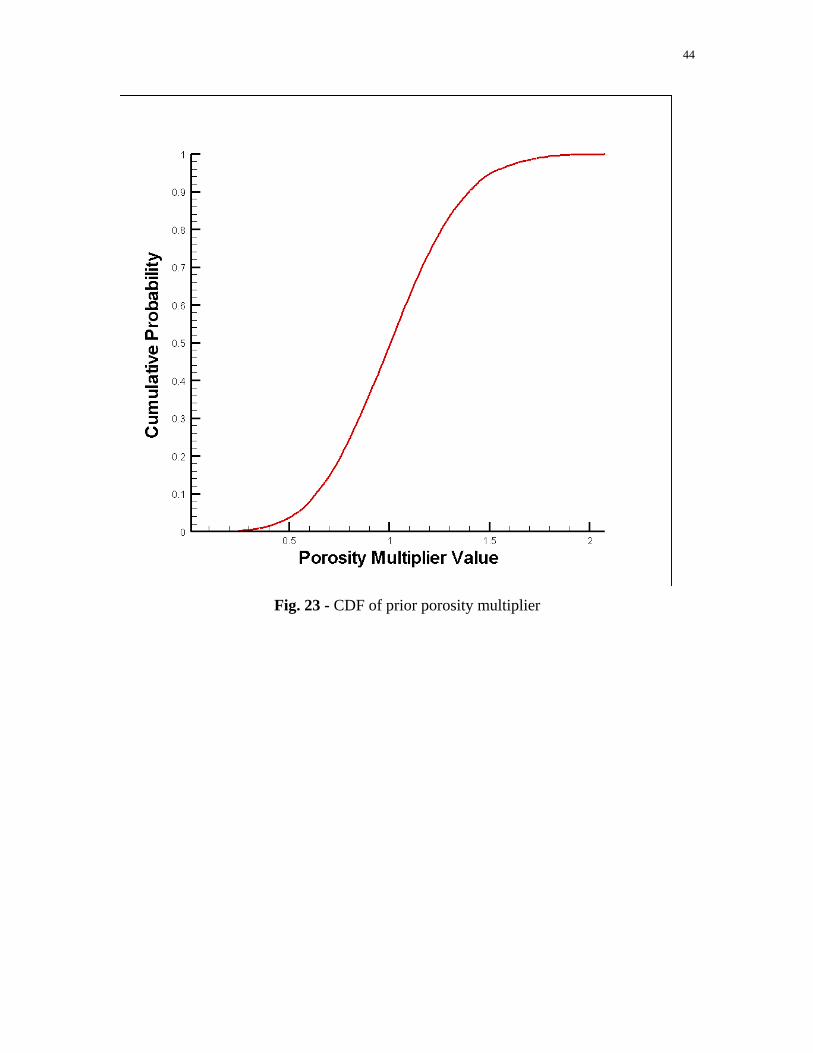
porosity was capped with a maximum value of 2.28 and minimum value of 0. Fig. 21 and

Fig. 22 show histograms of our prior porosity multiplier distribution and permeability

multiplier distribution. This sample size is 20,000 points. Also, the cumulative

distribution functions are shown by Fig. 23 and Fig. 24.

0

500

1000

1500

2000

2500

3000

0 0.1 0.2 0.3 0.4 0.5 0.6 0.7 0.8 0.9 1 1.1 1.2 1.3 1.4 1.5 1.6 1.7 1.8 1.9 2 2.1 2.2 2.28

Porosity Multiplier Value

Freq

uenc

y

Fig. 21 - Histogram of prior porosity multiplier distribution

43

0

500

1000

1500

2000

2500

00.1

5 0.3 0.45 0.6 0.7

5 0.9 1.05 1.2 1.3

5 1.5 1.65 1.8 1.9

5 2.1 2.25 2.4 2.5

5 2.7 2.85 3

3.15 3.3 3.4

5 3.6 3.75 3.9 4

Permeability Multiplier value

Freq

uenc

y

Fig. 22 - Histogram of prior permeability multiplier distribution

44

Fig. 23 - CDF of prior porosity multiplier

45

Fig. 24 - CDF of prior permeability multiplier

In order to simplify the equation derivation for the log-normal permeability multiplier, in

the MCMC history match process, the permeability multiplier was transferred back to a

logarithm form in order to be consistent with porosity multiplier which follows a normal

distribution. With the known ( )kXMedian as 1 and ( )kXVar as 235.1 and Eqs. 13-14,

the mean and standard deviation for the logarithm form permeability multiplier can be

calculated as 0log =KXμ , 354.0log =

kXσ . Together with the porosity multipliers, the prior

90 parameters distribution is shown by Eq. 15.

46

( ) ( )( )kXeXMedian klog10ln μ= ……………………………………………………………..…… (13)

( ) ( )( ) ( )( ) ( )( )2loglog2

log 10ln10ln210ln 1 kXkXkX eeXVar kσμσ +⎟

⎠⎞⎜

⎝⎛ −= ………………………………. (14)

( ) ( ) ( )⎟⎠⎞

⎜⎝⎛ −−−∝ − μμ XCXXP x

T 1

21exp ……………………………………………... (15)

⎥⎥⎥⎥⎥⎥⎥⎥⎥⎥⎥⎥⎥⎥⎥⎥⎥

⎦

⎤

⎢⎢⎢⎢⎢⎢⎢⎢⎢⎢⎢⎢⎢⎢⎢⎢⎢

⎣

⎡

=

30

2

1

60

2

1

.

.

.

log...

loglog

φ

φ

φ

X

XXX

XX

X k

k

k

....................................................................................................... (16)

Where kXlog is the logarithm multiplier of permeability and φX is the multiplier of

porosity. The total number of parameters is 90. xC is a diagonal matrix shown below

because each multiplier is considered independent in our study.

47

⎥⎥⎥⎥⎥⎥⎥⎥⎥⎥⎥⎥⎥⎥⎥⎥⎥⎥

⎦

⎤

⎢⎢⎢⎢⎢⎢⎢⎢⎢⎢⎢⎢⎢⎢⎢⎢⎢⎢

⎣

⎡

=

2

2

2

2log

2log

2log

..

.

..

.

φ

φ

φ

σ

σσ

σ

σσ

X

X

X

X

X

X

xk

k

k

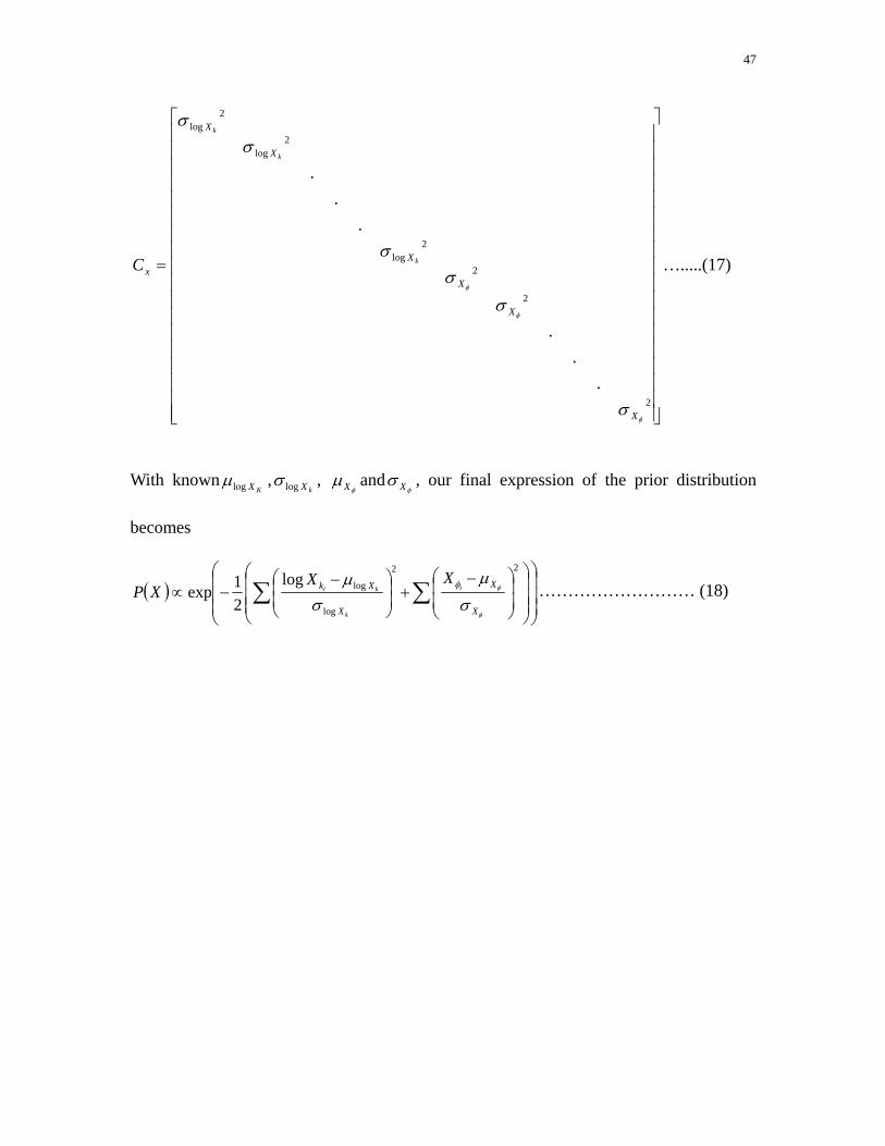
C ….....(17)

With knownKXlogμ ,

kXlogσ , φ

μX andφ

σ X , our final expression of the prior distribution

becomes

( )⎟⎟⎟

⎠

⎞

⎜⎜⎜

⎝

⎛

⎟⎟⎟

⎠

⎞

⎜⎜⎜

⎝

⎛

⎟⎟⎠

⎞⎜⎜⎝

⎛ −+⎟

⎟⎠

⎞⎜⎜⎝

⎛ −−∝ ∑ ∑

22

log

loglog21exp

φ

φ

σμ

σμ φ

X

X

X

Xk i

k

kiXX

XP ……………………… (18)

48

STATIC RESERVOIR STUDY

Overview

With the prior distribution defined as described above, the first test was carried out by

using the static MCMC method. This method is similar to the traditional application of

the MCMC method in a one-time study in which there is no adding of new dynamic data

during the history matching process. There are two main reasons for doing the static test

on the PUNQ-S3 model. First, we can compare our results with other previous work done

on this model. This is done in order to verify that our reservoir model was constructed

correctly and the prior distribution was chosen properly. Second, it lays the foundation

for doing the continuous case.

The likelihood function is also needed in order to construct our posterior distribution.

Using the MCMC method to explore the parameter space in our posterior distribution, we

can make a cumulative oil production forecast with all sampled models. I will describe

the details below.

The Likelihood Function

The definition of the likelihood function relies on the specification of a model for the

uncertainty around the observed production (Bos 1999). In our study, the measurement

errors are assumed to be an independent Gaussian distribution. Thus, our likelihood

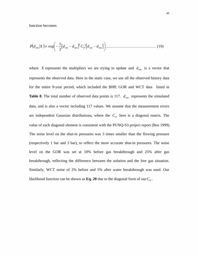
49

function becomes

( ) [ ] [ ]⎟⎠⎞

⎜⎝⎛ −−−∝ −

obssimDT

obssimobs ddCddXdP 1

21exp ………………………………… (19)

where X represents the multipliers we are trying to update and obsd is a vector that

represents the observed data. Here in the static case, we use all the observed history data

for the entire 9-year period, which included the BHP, GOR and WCT data listed in

Table 8. The total number of observed data points is 117. simd represents the simulated

data, and is also a vector including 117 values. We assume that the measurement errors

are independent Gaussian distributions, where the DC here is a diagonal matrix. The

value of each diagonal element is consistent with the PUNQ-S3 project report (Bos 1999).

The noise level on the shut-in pressures was 3 times smaller than the flowing pressure

(respectively 1 bar and 3 bar), to reflect the more accurate shut-in pressures. The noise

level on the GOR was set at 10% before gas breakthrough and 25% after gas

breakthrough, reflecting the difference between the solution and the free gas situation.

Similarly, WCT noise of 2% before and 5% after water breakthrough was used. Our

likelihood function can be shown as Eq. 20 due to the diagonal form of our DC .

50

Table 8 - Observed data in static case

Times(days) WBHP(BARSA) WGOR( 33 / SmSm ) WWCT( 33 / SmSm )

1.01 6 - -

91 6 - -

182 6 - -

274 6 - -

366 6 - -

1461 6 - -

1642 - 1 -

1826 6 5 -

1840 6 - -

1841 - 1 -

2008 - 2 -

2192 6 4 -

2206 6 - -

2373 - 2 -

2557 6 4 -

2571 6 - -

2572 - - 1

2738 - 2 1

2922 6 4 6

2936 6 - -

( ) ( )⎟⎟

⎠

⎞

⎜⎜

⎝

⎛⎟⎟⎠

⎞⎜⎜⎝

⎛ −−∝ ∑

=

2117

1

)(

21exp

i i

isimiobsobs

ddXdP

σ………………………………………. (20)

The Posterior Distribution

Our posterior distribution was constructed under the Bayesian frame based on the prior

51

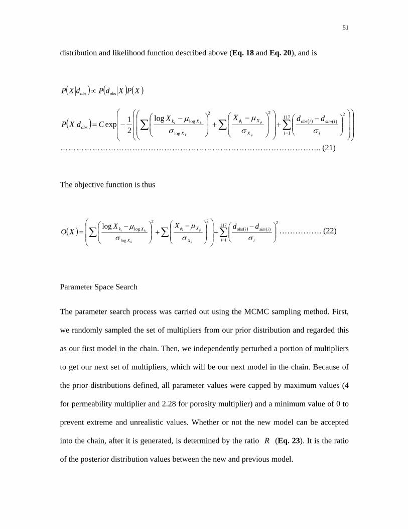
distribution and likelihood function described above (Eq. 18 and Eq. 20), and is

( ) ( ) ( )XPXdPdXP obsobs ∝

( ) ( )

⎟⎟⎟

⎠

⎞

⎜⎜⎜

⎝

⎛

⎟⎟⎟

⎠

⎞

⎜⎜⎜

⎝

⎛

⎟⎟⎠

⎞⎜⎜⎝

⎛ −+

⎟⎟⎟

⎠

⎞

⎜⎜⎜

⎝

⎛

⎟⎟⎠

⎞⎜⎜⎝

⎛ −+⎟

⎟⎠

⎞⎜⎜⎝

⎛ −−= ∑∑ ∑

=

2117

1

)(

22

log

loglog21exp

i i

isimiobs

X

X

X

Xkobs

ddXXCdXP i

k

ki

σσμ

σμ

φ

φφ

…………………………………………………………………………………….. (21)

The objective function is thus

( ) ( )2117

1

)(

22

log

loglog∑∑ ∑=

⎟⎟⎠

⎞⎜⎜⎝

⎛ −+⎟⎟⎟

⎠

⎞

⎜⎜⎜

⎝

⎛

⎟⎟⎠

⎞

⎜⎜⎝

⎛ −+⎟

⎟⎠

⎞⎜⎜⎝

⎛ −=

i i

isimiobs

X

X

X

Xk ddXXXO i

k

ki

σσμ

σμ

φ

φφ ……………. (22)

Parameter Space Search

The parameter search process was carried out using the MCMC sampling method. First,

we randomly sampled the set of multipliers from our prior distribution and regarded this

as our first model in the chain. Then, we independently perturbed a portion of multipliers

to get our next set of multipliers, which will be our next model in the chain. Because of

the prior distributions defined, all parameter values were capped by maximum values (4

for permeability multiplier and 2.28 for porosity multiplier) and a minimum value of 0 to

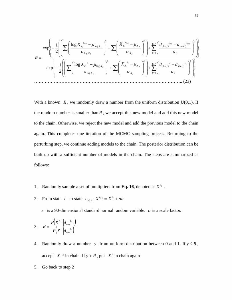
prevent extreme and unrealistic values. Whether or not the new model can be accepted

into the chain, after it is generated, is determined by the ratio R (Eq. 23). It is the ratio

of the posterior distribution values between the new and previous model.

52

( )

( )

⎪⎭

⎪⎬

⎫

⎪⎩

⎪⎨

⎧

⎟⎟⎟

⎠

⎞

⎜⎜⎜

⎝

⎛

⎟⎟⎠

⎞⎜⎜⎝

⎛ −+

⎟⎟⎟

⎠

⎞

⎜⎜⎜

⎝

⎛

⎟⎟

⎠

⎞

⎜⎜

⎝

⎛ −+⎟

⎟⎠

⎞⎜⎜⎝

⎛ −−

⎪⎭

⎪⎬

⎫

⎪⎩

⎪⎨

⎧

⎟⎟⎟

⎠

⎞

⎜⎜⎜

⎝

⎛

⎟⎟⎠

⎞⎜⎜⎝

⎛ −+

⎟⎟⎟

⎠

⎞

⎜⎜⎜

⎝

⎛

⎟⎟

⎠

⎞

⎜⎜

⎝

⎛ −+⎟

⎟⎠

⎞⎜⎜⎝

⎛ −−

=

∑∑ ∑

∑∑ ∑

=

=

++++

2117

1

)(

22

log

log

2117

1

)(

22

log

log

log21exp

log21exp

1111

i i

tisim

tiobs

X

Xt

X

Xt

k

i i

tisim

tiobs

X

Xt

X

Xt

k

iii

i

k

k

i

i

iii

i

k

k

i

i

ddXX

ddXX

R

σσμ

σμ

σσμ

σμ

φ

φ

φ

φ

φ

φ

…………………………………………………………………………………….. (23)

With a known R , we randomly draw a number from the uniform distribution U(0,1). If

the random number is smaller than R , we accept this new model and add this new model

to the chain. Otherwise, we reject the new model and add the previous model to the chain

again. This completes one iteration of the MCMC sampling process. Returning to the

perturbing step, we continue adding models to the chain. The posterior distribution can be

built up with a sufficient number of models in the chain. The steps are summarized as

follows:

1. Randomly sample a set of multipliers from Eq. 16, denoted as 1tX .

2. From state it to state 1+it , σε+=+ ii tt XX 1

ε is a 90-dimensional standard normal random variable. σ is a scale factor.

3. ( )( )ii

ii

tobs

t

tobs

t

dXP

dXPR

11 ++

=

4. Randomly draw a number y from uniform distribution between 0 and 1. If Ry ≤ ,

accept 1+itX in chain. If Ry > , put itX in chain again.

5. Go back to step 2

53

In using this MCMC sampling process, it is very important to choose the scalar σ

properly and to decide how many parameters are perturbed each iteration. They directly

affect if our chain could mix well or converge fast with a reasonable acceptance rate. In

order to show how the acceptance rate affects the sampled distribution, tests were carried

out on the porosity multiplier of our prior distribution with a number of 10,000-sample

models. If the acceptance rate of the whole chain is too high, all the samples would

almost have the same values, which means the parameter space is only partially explored.

Fig. 25 shows the histograms comparison between a high acceptance rate ( %7.99 ) chain

and the truth case, which illustrates this point. On the other hand, if the acceptance rate of

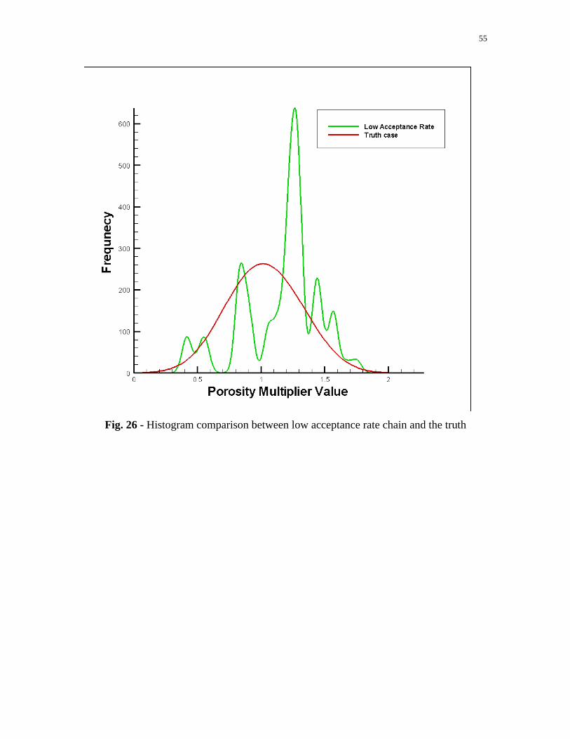
the whole chain is too low, the chain will be stuck on the same model for a long time. The

histogram cannot reproduce the shape of the probability density function with just a few

accepted models. Fig. 26 shows the histograms comparison between a low acceptance

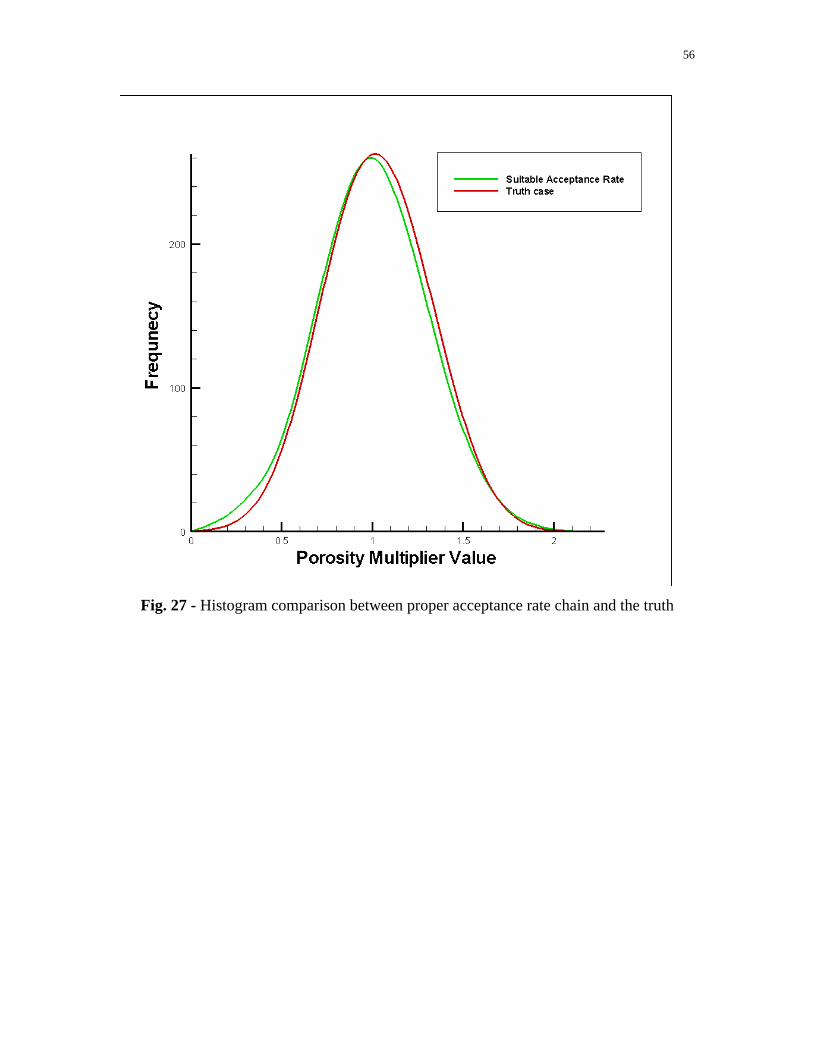
rate chain ( %2.3 ) and the truth case. In some experiments, we set the perturb scalar as

0.1 and perturbed 10 parameters at each time, obtaining an acceptance rate of

approximately %80 . With these MCMC parameters, our prior histogram reproduced the

truth case much closer (Fig. 27).

54

Fig. 25 - Histogram comparison between high acceptance rate chain and the truth

55

Fig. 26 - Histogram comparison between low acceptance rate chain and the truth

56

Fig. 27 - Histogram comparison between proper acceptance rate chain and the truth

57

Forecast

With the determined scalar value and a proper perturbation size of parameters, we can

now start to sample our models from a posterior distribution (Eq. 19). The acceptance

rate of the chain is approximately 40% when the likelihood term is included. This is also

a reasonable acceptance rate to ensure a well mixed chain (Givens and hoeting 2005). The

objective function value of the whole chain is shown by Fig. 28. The program is run to

get 17,400 samples, where we determine by observation that the chain is stable and long

enough to build up the posterior distribution. The first 7,000 models are determined

visually to be in the burn-in period and are eliminated from the chain. We use the rest of

the models to forecast the cumulative oil production at 16.5 years. Fig. 29 shows the

objective function value of all mixed-well models used to forecast. The forecast

histogram and cumulative distribution function are shown in Fig. 30 and Fig. 31,

respectively. Fig. 32 shows our results compared to previous published results.

58

Fig. 28 - Objective function value vs. model number (static case)

Burn in

59

Fig. 29 - Mixed well objective function value vs. model number (static case)

60

0

500

1000

1500

2000

2500

3000

3740000 3760000 3780000 3800000 3820000 3840000 3860000 3880000 3900000 3920000 3940000 3960000

Cumulative Oil Production at 16.5 years(SM3)

Freq

ency

Fig. 30 - Histogram of cumulative oil production made by static case

61

Fig. 31 - CDF of cumulative production by mixed well models in static case

Truth Case

62

3.4 3.3

3.5

3.6 3.73.8

3.9 4.0

4.14.2

3.2

TNO

-1TN

O-2

TNO

-3A

moc

o-is

oA

moc

o-en

iso

Elf

IFP

-STM

IFP

-Oliv

erN

CC

-Oliv

erN

CC

-GA

NC

C-M

CM

CE

nKF-

Initi

alE

nKF-

Cor

rect

edM

CM

C-S

tatic

Truth CaseC

umul

ativ

e P

rodu

ctio

n (S

M3*

10^6

)

PUBLISHED FORECASTS OUR RESULT

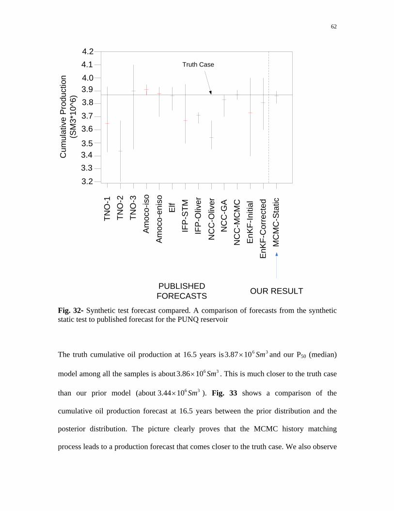
Fig. 32- Synthetic test forecast compared. A comparison of forecasts from the synthetic static test to published forecast for the PUNQ reservoir

The truth cumulative oil production at 16.5 years is 361087.3 Sm× and our P50 (median)

model among all the samples is about 361086.3 Sm× . This is much closer to the truth case

than our prior model (about 361044.3 Sm× ). Fig. 33 shows a comparison of the

cumulative oil production forecast at 16.5 years between the prior distribution and the

posterior distribution. The picture clearly proves that the MCMC history matching

process leads to a production forecast that comes closer to the truth case. We also observe

63

that our uncertainty range narrows significantly after doing the history matching process

(Fig. 33). The P10 model among all samples is about 361080.3 Sm× and the P90 model is

about 361090.3 Sm× .

Fig. 33 - CDF comparison between prior and posterior (static case)

64

In addition to providing probabilistic forecasts, we can also provide a probabilistic

assessment of reservoir properties by building up the multiplier distribution from our

sampled models. Such information could be valuable in routine reservoir management

tasks, such as infill drilling. In layers and regions where wells were completed, and thus

more dynamic data were available, the posterior distributions of parameters varied

significantly from the prior distribution. In layers and regions where wells were not

completed, the posterior distribution deviated only slightly from the prior distribution.

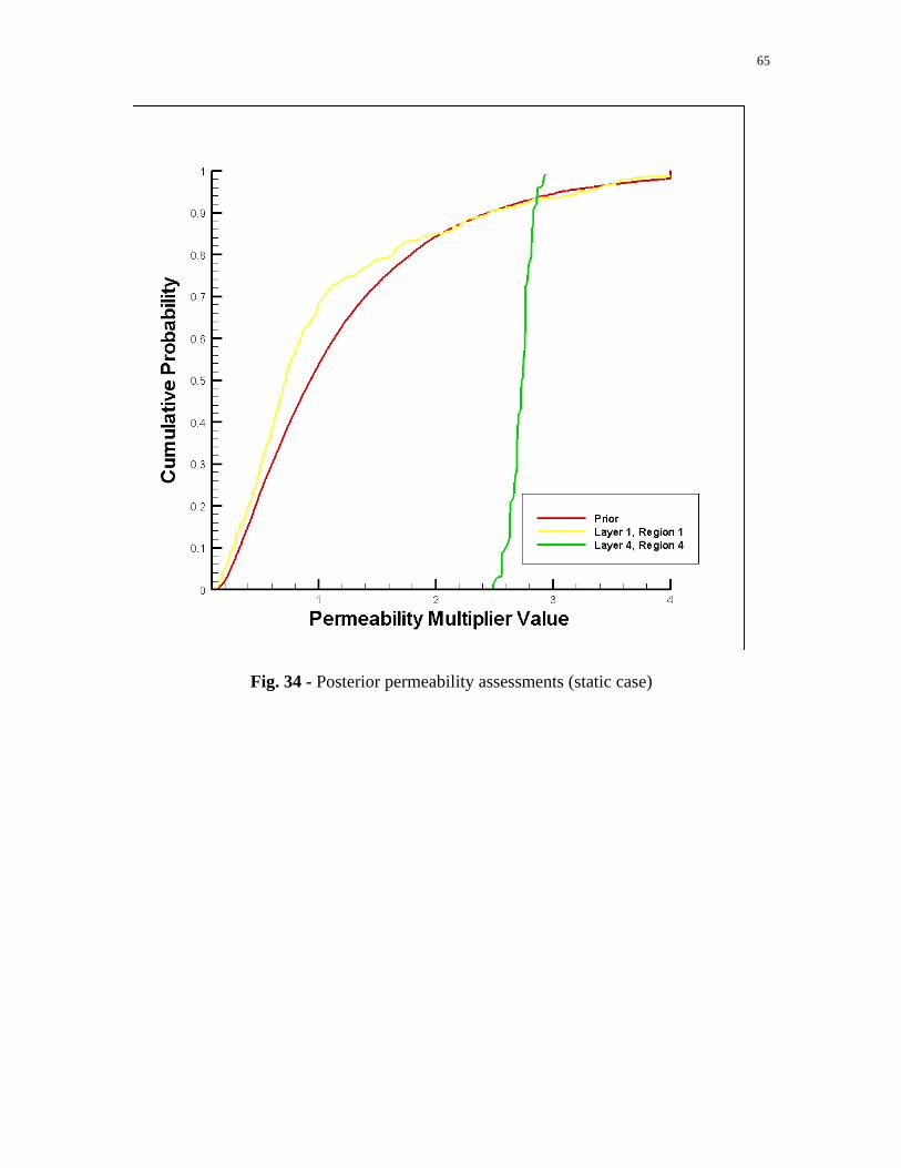
This is illustrated in Fig. 34, which shows the prior and posterior distributions of the

horizontal permeability multiplier in layer 1, region 1 (no wells) and layer 4, region 4

(where a well is completed). The posterior distribution of layer 4, region 4, deviates

significantly from the prior. Meanwhile, the posterior distribution in layer 1, region 1, is

quite similar to the prior distribution. This behavior is typical of the other regions in the

reservoir. Thus, the history matching process allows us to refine and narrow our

assessments of reservoir properties in only those regions and layers in which wells are

present and in which we have dynamic data available.

65

Fig. 34 - Posterior permeability assessments (static case)

66

Summary of Results

Close agreement between our static test forecast and the truth case demonstrates that the

initial model and prior distributions were set up properly. The difference between the

prior and posterior CDFs of the cumulative production forecast demonstrates the value of

the MCMC history matching process. The narrower uncertainty range after the history

match demonstrates that more information leads to less uncertainty. In addition, the test

shows that we can improve our assessments of reservoir properties. The static case also

provides a base for comparison for the continuous case discussed in the next section.

67

CONTINUOUS RESERVOIR STUDY

Overview

The second test was conducted on the PUNQ-S3 synthetic reservoir by using the

continuous MCMC method. An objective of developing this continuous technology is to

include the new observed data as soon as it becomes available, which could lead to a

better estimation of the underlying reservoir.

In this continuous history matching process, the simulation runs were also matched

against observed data for 9 years. The forecasts were made to 16.5 years of production.

The difference is that the PUNQ-S3 model was continuously simulated, starting from

year 4.5 and continuing through the end of year 9, making forecasts to 16.5 years. During

the test, the history data were added in sequence at the 5th, 6th, 7th, 8th and 9th years. For

the first half year (4.5 to 5 years), 4,500 models were sampled and the number of sampled

models was 9,000 per year for the remaining years. As a result, the total number of

simulation samples was 49,500. All of this assumes that 9000 model runs can be made in

a year of actual time. This equates to about one run per hour, which is not atypical in the

petroleum industry today for fieldwide simulation runs. Thus, the comparisons to be

made in this section are between static and continuous simulations at the end of year 10,

one year after the acquisition of the last observed data at the end of year 9.

In this continuous study, our uncertain parameters are also the 90 porosity and

68

permeability multipliers. The initial model and prior multiplier distribution are the same

as we used in our static test. As we add in the observed data sequentially, our likelihood

function (Eq. 19) changes when the new observed data are included. Compared to the

sampled models prior to adding in the new data, the later sampled models’ posterior

distribution would include more observed and simulated data. Results of these runs were

combined into probabilistic forecasts at the time points corresponding to the addition of

new observed data.

The Likelihood Function

In the continuous MCMC test, the history data are divided into six parts and the sampling

process starts in year 4.5. The new history data are added in sequentially; at the 5th, 6th, 7th,

8th and 9th years. Table 9 shows how we divided the history data.

69

Table 9 - Observed data in the continuous case (each color sequence corresponds to a

different data assimilation)

Time(days) WBHP(BARSA) WGOR( 33 / SmSm ) WWCT( 33 / SmSm )1.01 6 - - 91 6 - - 182 6 - - 274 6 - - 366 6 - - 1461 6 - -

1642(before 4.5 year) - 1 - 1826(before 5 year) 6 5 -

1840 6 - - 1841 - 1 - 2008 - 2 -

2192(before 6 year) 6 4 - 2206 6 - - 2373 - 2 -

2557(before 7 year) 6 4 - 2571 6 - - 2572 - - 1 2738 - 2 1

2922(before 8 year) 6 4 6 2936(before 9 year) 6 - -

Recall that Eq. 20 shows the likelihood function with all history data in the static case.

Here, Eqs. 24-29 represent the likelihood functions used in 4.5th, 5th, 6th, 7th, 8th and 9th

years, respectively.

( ) ( )⎟⎟

⎠

⎞

⎜⎜

⎝

⎛⎟⎟⎠

⎞⎜⎜⎝

⎛ −−∝ ∑

=

237

1

)(

21exp

i i

isimiobsobs

ddXdP

σ……………………………………….. (24)

( ) ( )⎟⎟

⎠

⎞

⎜⎜

⎝

⎛⎟⎟⎠

⎞⎜⎜⎝

⎛ −−∝ ∑

=

248

1

)(

21exp

i i

isimiobsobs

ddXdP

σ……………………………………….. (25)

70

( ) ( )⎟⎟

⎠

⎞

⎜⎜

⎝

⎛⎟⎟⎠

⎞⎜⎜⎝

⎛ −−∝ ∑

=

267

1

)(

21exp

i i

isimiobsobs

ddXdP

σ……………………………………….. (26)

( ) ( )⎟⎟

⎠

⎞

⎜⎜

⎝

⎛⎟⎟⎠

⎞⎜⎜⎝

⎛ −−∝ ∑

=

285

1

)(

21exp

i i

isimiobsobs

ddXdP

σ……………………………………...… (27)

( ) ( )⎟⎟

⎠

⎞

⎜⎜

⎝

⎛⎟⎟⎠

⎞⎜⎜⎝

⎛ −−∝ ∑

=

2111

1

)(

21exp

i i

isimiobsobs

ddXdP

σ………...……………………………… (28)

( ) ( )⎟⎟

⎠

⎞

⎜⎜

⎝

⎛⎟⎟⎠

⎞⎜⎜⎝

⎛ −−∝ ∑

=

2117

1

)(

21exp

i i

isimiobsobs

ddXdP

σ…...…………………………………… (29)

The Posterior Distribution

Due to the changes we have made in the likelihood function, the posterior distributions in

different years also differ from each other. Eq. 21 shows the posterior distribution with all

9 year’s history data in the static case. Here, Eqs. 30-35 represent the posterior

distribution used in 4.5th, 5th, 6th, 7th, 8th and 9th years, respectively.

( ) ( )

⎟⎟⎟

⎠

⎞

⎜⎜⎜

⎝

⎛

⎟⎟⎟

⎠

⎞

⎜⎜⎜

⎝

⎛

⎟⎟⎠

⎞⎜⎜⎝

⎛ −+⎟⎟⎟

⎠

⎞

⎜⎜⎜

⎝

⎛

⎟⎟⎠

⎞⎜⎜⎝

⎛ −+⎟

⎟⎠

⎞⎜⎜⎝

⎛ −−= ∑∑ ∑

=

237

1

)(

22

log

loglog21exp

i i

isimiobs

X

X

X

Xkobs

ddXXCdXP i

k

ki

σσμ

σμ

φ

φφ

………………………………………..…………………………………………… (30)

( ) ( )

⎟⎟⎟

⎠

⎞

⎜⎜⎜

⎝

⎛

⎟⎟⎟

⎠

⎞

⎜⎜⎜

⎝

⎛

⎟⎟⎠

⎞⎜⎜⎝

⎛ −+⎟⎟⎟

⎠

⎞

⎜⎜⎜

⎝

⎛

⎟⎟⎠

⎞⎜⎜⎝

⎛ −+⎟

⎟⎠

⎞⎜⎜⎝

⎛ −−= ∑∑ ∑

=

248

1

)(

22

log

loglog21exp

i i

isimiobs

X

X

X

Xkobs

ddXXCdXP i

k

ki

σσμ

σμ

φ

φφ

………………………………..…………………………………………………… (31)

( ) ( )

⎟⎟⎟

⎠

⎞

⎜⎜⎜

⎝

⎛

⎟⎟⎟

⎠

⎞

⎜⎜⎜

⎝

⎛

⎟⎟⎠

⎞⎜⎜⎝

⎛ −+⎟⎟⎟

⎠

⎞

⎜⎜⎜

⎝

⎛

⎟⎟⎠

⎞⎜⎜⎝

⎛ −+⎟

⎟⎠

⎞⎜⎜⎝

⎛ −−= ∑∑ ∑

=

267

1

)(

22

log

loglog21exp

i i

isimiobs

X

X

X

Xkobs

ddXXCdXP i

k

ki

σσμ

σμ

φ

φφ

……………………………………..……………………………………………… (32)

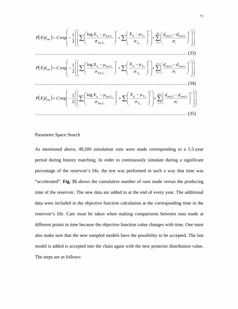
71

( ) ( )

⎟⎟⎟

⎠

⎞

⎜⎜⎜

⎝

⎛

⎟⎟⎟

⎠

⎞

⎜⎜⎜

⎝

⎛

⎟⎟⎠

⎞⎜⎜⎝

⎛ −+⎟⎟⎟

⎠

⎞

⎜⎜⎜

⎝

⎛

⎟⎟⎠

⎞⎜⎜⎝

⎛ −+⎟

⎟⎠

⎞⎜⎜⎝

⎛ −−= ∑∑ ∑

=

285

1

)(

22

log

loglog21exp

i i

isimiobs

X

X

X

Xkobs

ddXXCdXP i

k

ki

σσμ

σμ

φ

φφ

………………………………..…………………………………………………… (33)

( ) ( )

⎟⎟⎟

⎠

⎞

⎜⎜⎜

⎝

⎛

⎟⎟⎟

⎠

⎞

⎜⎜⎜

⎝

⎛

⎟⎟⎠

⎞⎜⎜⎝

⎛ −+⎟⎟⎟

⎠

⎞

⎜⎜⎜

⎝

⎛

⎟⎟⎠

⎞⎜⎜⎝

⎛ −+⎟

⎟⎠

⎞⎜⎜⎝

⎛ −−= ∑∑ ∑

=

2111

1

)(

22

log

loglog21exp

i i

isimiobs

X

X

X

Xkobs

ddXXCdXP i

k

ki

σσμ

σμ

φ

φφ

……………………………………………..……………………………………… (34)

( ) ( )

⎟⎟⎟

⎠

⎞

⎜⎜⎜

⎝

⎛

⎟⎟⎟

⎠

⎞

⎜⎜⎜

⎝

⎛

⎟⎟⎠

⎞⎜⎜⎝

⎛ −+

⎟⎟⎟

⎠

⎞

⎜⎜⎜

⎝

⎛

⎟⎟⎠

⎞⎜⎜⎝

⎛ −+⎟

⎟⎠

⎞⎜⎜⎝

⎛ −−= ∑∑ ∑

=

2117

1

)(

22

log

loglog21exp

i i

isimiobs

X

X

X

Xkobs

ddXXCdXP i

k

ki

σσμ

σμ

φ

φφ

…………………………………………………..………………………………… (35)

Parameter Space Search

As mentioned above, 49,500 simulation runs were made corresponding to a 5.5-year

period during history matching. In order to continuously simulate during a significant

percentage of the reservoir’s life, the test was performed in such a way that time was

“accelerated”. Fig. 35 shows the cumulative number of runs made versus the producing

time of the reservoir. The new data are added in at the end of every year. The additional

data were included in the objective function calculation at the corresponding time in the

reservoir’s life. Care must be taken when making comparisons between runs made at

different points in time because the objective function value changes with time. One must

also make sure that the new sampled models have the possibility to be accepted. The last

model is added is accepted into the chain again with the new posterior distribution value.

The steps are as follows:

72

1. Randomly sample a set of multiplier from Eq. 18, denoted as 1tX .

2. From state it to state 1+it , σε+=+ ii tt XX 1

ε is a 90-dimensional standard normal random variable. σ is a scalar factor.

3. ( )( )ii

ii

tobs

t

tobs

t

dXP

dXPR

11 ++

=

4. Randomly draw a number y from uniform distribution between 0 and 1. If Ry ≤ ,

accept 1+itX in chain. If Ry > , put itX in chain again.

5. Check to see if new observed data are available. If yes, recalculate the last model in

the chain with the new posterior distribution function and go to step 2. If no, go

directly to step 2.

Additionally, in order to make the chain converge fast and mix well, the scalar and

perturbation size used in the continuous case are the same as those used in the static case.

73

0

5000

10000

15000

20000

25000

30000

35000

40000

45000

50000

0 1 2 3 4 5 6 7 8 9 10

Reservior Life, years

Sim

ulat

ion

Run

Num

ber

Fig. 35 - Continuous test run number by time. Run number versus point in reservoir life for the continuous test

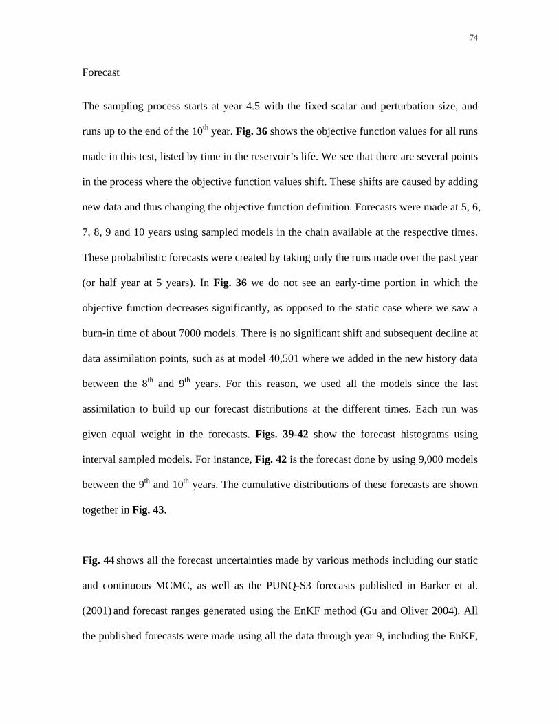
74

Forecast

The sampling process starts at year 4.5 with the fixed scalar and perturbation size, and

runs up to the end of the 10th year. Fig. 36 shows the objective function values for all runs

made in this test, listed by time in the reservoir’s life. We see that there are several points

in the process where the objective function values shift. These shifts are caused by adding

new data and thus changing the objective function definition. Forecasts were made at 5, 6,

7, 8, 9 and 10 years using sampled models in the chain available at the respective times.

These probabilistic forecasts were created by taking only the runs made over the past year

(or half year at 5 years). In Fig. 36 we do not see an early-time portion in which the

objective function decreases significantly, as opposed to the static case where we saw a

burn-in time of about 7000 models. There is no significant shift and subsequent decline at

data assimilation points, such as at model 40,501 where we added in the new history data

between the 8th and 9th years. For this reason, we used all the models since the last

assimilation to build up our forecast distributions at the different times. Each run was

given equal weight in the forecasts. Figs. 39-42 show the forecast histograms using

interval sampled models. For instance, Fig. 42 is the forecast done by using 9,000 models

between the 9th and 10th years. The cumulative distributions of these forecasts are shown

together in Fig. 43.

Fig. 44 shows all the forecast uncertainties made by various methods including our static

and continuous MCMC, as well as the PUNQ-S3 forecasts published in Barker et al.

(2001) and forecast ranges generated using the EnKF method (Gu and Oliver 2004). All

the published forecasts were made using all the data through year 9, including the EnKF,

75

except for the continuous MCMC yearly forecasts with different history data. The median

of our forecast made between the 9th and 10th years, which includes all the history data, is

pretty close to the truth case. Also, from Fig. 44, we can tell our continuous result is

comparable to NCC-MCMC method because of the similar uncertainty rage. This

happens as well as the traditional MCMC method.

We can draw some general conclusions from Fig. 44. First, we see the medians of our

forecasts are moving from the median of the prior distribution ( 361044.3 Sm× made by

the initial model) towards the truth case. This happens year by year while adding in more

yearly history data. This is because the likelihood term in our posterior distribution is

assuming more weight with more observed data, which will lead the forecast result from

prior model to the truth case by involving more history information. Second, we see that

as time progresses, the uncertainty range narrows and shifts. This shows the newly

observed data are of value because they alter our assessments. The narrowing and shifting

are more obvious in the early years’ forecasts, which also seems reasonable. Early on, the

observed data set included in our posterior distribution is smaller and, thus, each new

available data point will have a larger impact on the posterior distribution. As the data set

becomes larger, the impact of new available data during the later year decreases. The

uncertainty range narrows as more data are assimilated. This makes sense, as we would

expect the uncertainty to decrease as we acquire more information about the reservoir.

Fig. 44 shows the production forecasts with all the history data made by the static and

continuous cases (between the 9th and 10th years). Even though both are similar and close

76

to the truth case, the comparison is not quite fair because the static case is using many

more sampled models to build up the uncertainty range as opposed to the continuous case.

In the static case, we ran 17,400 models and used the last 10,400 models to forecast the

uncertainty, considering the first 7000 models to be the burn-in period. In our continuous

case, we simply used all 9,000 models sampled from the beginning of the 9th year. This

saved almost a year’s worth of simulation runs and yielded a slightly better forecast

(smaller uncertainty) than the static case. If we want to compare forecasts at the end of

the 10th year, we can only make a fair comparison by using the 9,000 models sampled

from the continuous case and the first 9,000 models from our static case (assuming only

9000 simulation runs can be made in year). Fig. 45 shows the objective function

comparison for these two cases, while Fig. 46 shows the cumulative production vs. model

number. Fig. 47 shows the CDFs of static case and continuous case by using 9,000

models.

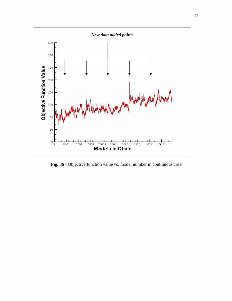
77

Fig. 36 - Objective function value vs. model number in continuous case

New data added points

78

0

200

400

600

800

1000

1200

1400

1600

1800

2000

3300000 3400000 3500000 3600000 3700000 3800000 3900000 4000000


Freq

uenc

y

Fig. 37 - Synthetic test forecast using model between 4.5 to 5 years (runs 1-4,500)

0

500

1000

1500

2000

2500

3000

3300000 3400000 3500000 3600000 3700000 3800000 3900000 4000000


Freq

uenc

y

Fig. 38 - Synthetic test forecast using model between 5 to 6 years (runs 4,501-13,500)

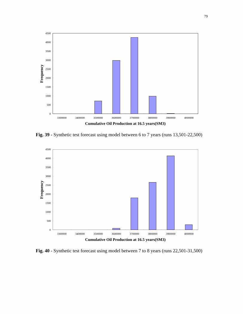
79

0

500

1000

1500

2000

2500

3000

3500

4000

4500

3300000 3400000 3500000 3600000 3700000 3800000 3900000 4000000


Freq

uenc

y


0

500

1000

1500

2000

2500

3000

3500

4000

4500

3300000 3400000 3500000 3600000 3700000 3800000 3900000 4000000


Freq

uenc

y


80

0

1000

2000

3000

4000

5000

6000

7000

3300000 3400000 3500000 3600000 3700000 3800000 3900000 4000000


Freq

uenc

y


0

1000

2000

3000

4000

5000

6000

7000

3300000 3400000 3500000 3600000 3700000 3800000 3900000 4000000


Freq

uenc

y


81

Fig. 43 - Continuous test forecast CDFs. A comparison of the cumulative distribution functions for various forecasts made during each year (or half year)

Truth case

82

Fig. 44 - Synthetic test forecast compared. A comparison of forecasts from the synthetic continuous test to published forecast for the PUNQ reservoir

83

Fig. 45 - Comparison of objective function value between static case and continuous case, with 9,000 models made between years 9 and 10

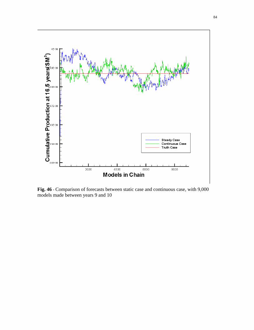
84

Fig. 46 - Comparison of forecasts between static case and continuous case, with 9,000 models made between years 9 and 10

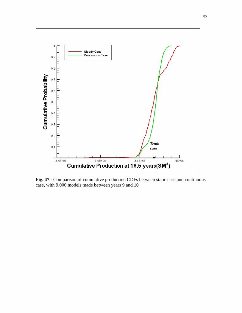
85

Fig. 47 - Comparison of cumulative production CDFs between static case and continuous case, with 9,000 models made between years 9 and 10

Truth case

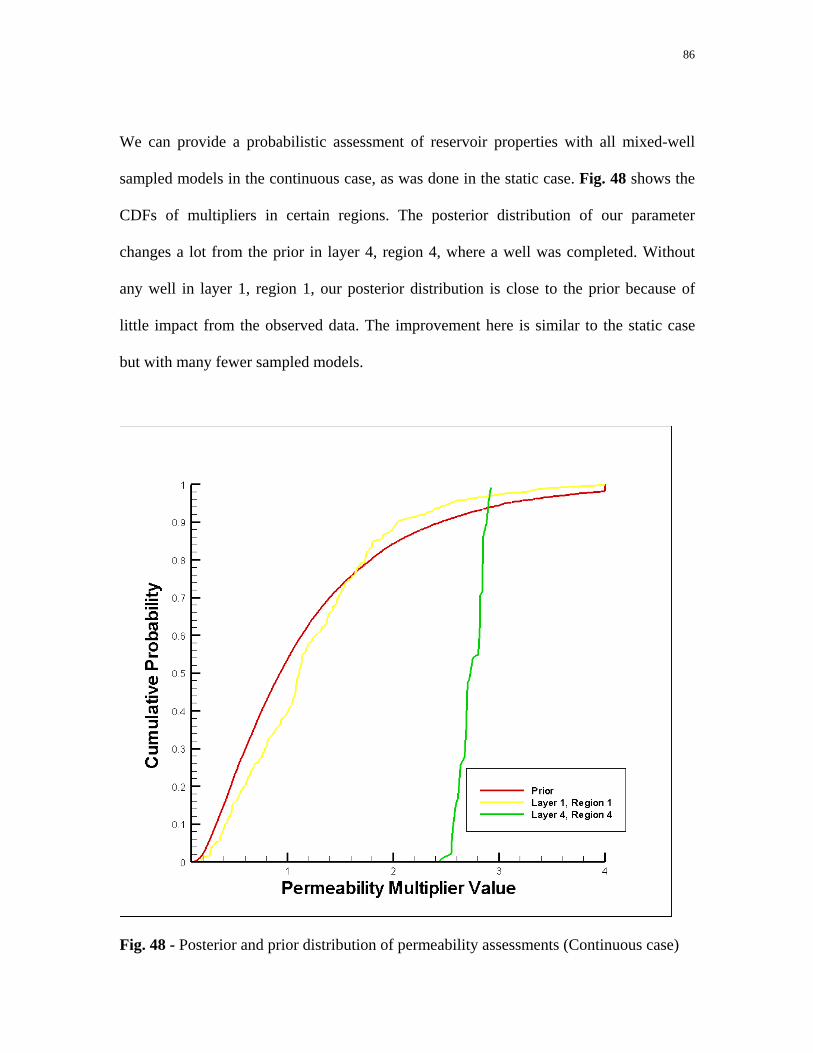
86

We can provide a probabilistic assessment of reservoir properties with all mixed-well

sampled models in the continuous case, as was done in the static case. Fig. 48 shows the

CDFs of multipliers in certain regions. The posterior distribution of our parameter

changes a lot from the prior in layer 4, region 4, where a well was completed. Without

any well in layer 1, region 1, our posterior distribution is close to the prior because of

little impact from the observed data. The improvement here is similar to the static case

but with many fewer sampled models.

Fig. 48 - Posterior and prior distribution of permeability assessments (Continuous case)

87

Consider a more practical problem, one in which we want to generate a forecast CDF at a

time when we do not have enough samples available since the data assimilation. There is

more like what the continuous simulation process will be like in an actual field

application, where the data acquisition rate is likely to be higher than the once per year

assumed in the tests described thus far. In this situation, since the chain will likely not be

long enough to build up the correct distribution, we will have to also rely on models

sampled from previous years to build up the distribution. Fig. 49 shows the CDFs

obtained by combining two years of sampled models together. We can see the truth case

still falls in the range of forecasts in the later years and the distributions move toward the

truth case and narrow as in the forecasts obtained using only one year of models. Since

the distributions were built up with samples over two years, models are sampled with

different objective functions. Fig. 50 shows an extreme case where the CDFs are obtained

using all models from previous years for each forecast. Though the truth case falls in the

range except for the first half year, the uncertainty range does not narrow as much over

time because we retain all the uncertainty from all the previous years. In actual field

applications where the data assimilation rate is much higher than we have assumed, the

question remains of how many models back should be retained to generate reasonable

posterior distributions. This will require a balance between retaining many samples

(resulting in longer chains) versus retaining fewer samples (more uniform objective

function definition).

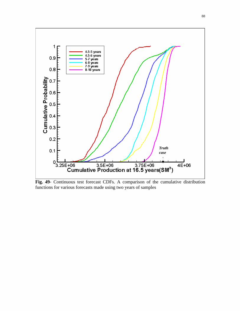
88

Fig. 49- Continuous test forecast CDFs. A comparison of the cumulative distribution functions for various forecasts made using two years of samples

Truth case

89

Fig. 50- Continuous test forecast CDFs. A comparison of the cumulative distribution functions for various forecasts made using all the models in previous years

Calibration of Uncertainty Estimates

Referring back to Fig. 44, we see that the first three forecasts failed to bracket the truth

case, and the forecast made between 4.5 and 5 years is particularly far off. Thus, the

uncertainty is underestimated in the early years. This could be due to either an

underestimation of uncertainty in the prior distribution, or an underestimation in the error

in the observed data. We would like to correctly quantify the uncertainty at all times,

even when there is not much dynamic data available. In order to increase the uncertainty,

Truth case

90

we can use a larger standard deviation in either our prior distribution or the observed data,

or both. I increased the standard deviations of our prior multipliers in order to overcome

this drawback. The permeability multiplier standard deviation was increased from 0..354

to 1 and the porosity multiplier standard deviation was increased from 0.3 to 0.5. Figs.

51-56 show the forecasts generated using one year’s worth of models and the enlarged

prior distributions, while Fig. 57 shows the CDFs of cumulative production for all the

forecasts. Fig. 58 summarizes the uncertainty ranges and compares them to the forecasts

with the original prior distribution. Compared to the forecasts with the original prior, the

enlarged prior standard deviation yields larger uncertainty ranges in the early year which

bracket the truth case (between 4.5 and 5 years and between 5 and 6 years). The forecasts

in the later years, however, are similar because of the larger impact of the likelihood

function (observed data) in later years.

These results suggest another benefit of the continuous simulation approach – calibration

of uncertainty estimates. However, our test was a synthetic test in which we know the

truth case. Since we know the truth case, we could adjust the prior distribution until all

the forecasts bracketed the truth case. How could this work in an actual field application

in which we do not know the correct answer? The solution is suggested in Fig. 58. With

the original prior, the posterior distributions shift in addition to narrowing. Subsequent

distributions are not bracketed by previous distributions. In the enlarged prior case,

however, subsequent distributions are essentially bracketed by all previous distributions,

which is what we should expect to see in practice. To effect this in a continuous

simulation application, one must monitor the posterior distributions generated over time.

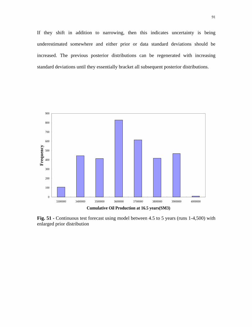
91

If they shift in addition to narrowing, then this indicates uncertainty is being

underestimated somewhere and either prior or data standard deviations should be

increased. The previous posterior distributions can be regenerated with increasing

standard deviations until they essentially bracket all subsequent posterior distributions.

0

100

200

300

400

500

600

700

800

900

3300000 3400000 3500000 3600000 3700000 3800000 3900000 4000000


Freq

uenc

y

Fig. 51 - Continuous test forecast using model between 4.5 to 5 years (runs 1-4,500) with enlarged prior distribution

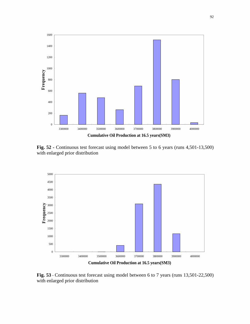
92

0

200

400

600

800

1000

1200

1400

1600

3300000 3400000 3500000 3600000 3700000 3800000 3900000 4000000


Freq

uenc

y

Fig. 52 - Continuous test forecast using model between 5 to 6 years (runs 4,501-13,500) with enlarged prior distribution

0

500

1000

1500

2000

2500

3000

3500

4000

4500

5000

3300000 3400000 3500000 3600000 3700000 3800000 3900000 4000000


Freq

uenc

y


93

0

500

1000

1500

2000

2500

3000

3300000 3400000 3500000 3600000 3700000 3800000 3900000 4000000


Freq

uenc

y


0

500

1000

1500

2000

2500

3000

3500

4000

4500

3300000 3400000 3500000 3600000 3700000 3800000 3900000 4000000


Freq

uenc

y


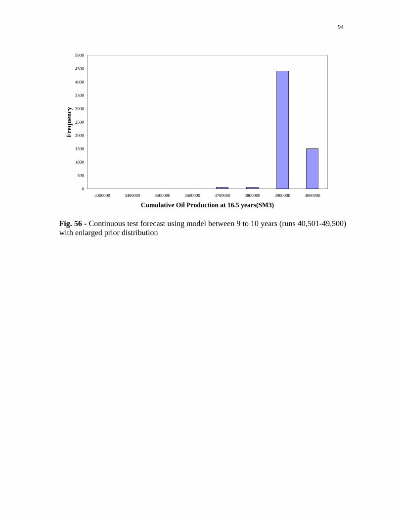
94

0

500

1000

1500

2000

2500

3000

3500

4000

4500

5000

3300000 3400000 3500000 3600000 3700000 3800000 3900000 4000000


Freq

uenc

y


95

Fig. 57 - Continuous test forecast CDFs with enlarged prior. A comparison of the cumulative distribution functions for various forecast made during each year (or half year)

Truth case

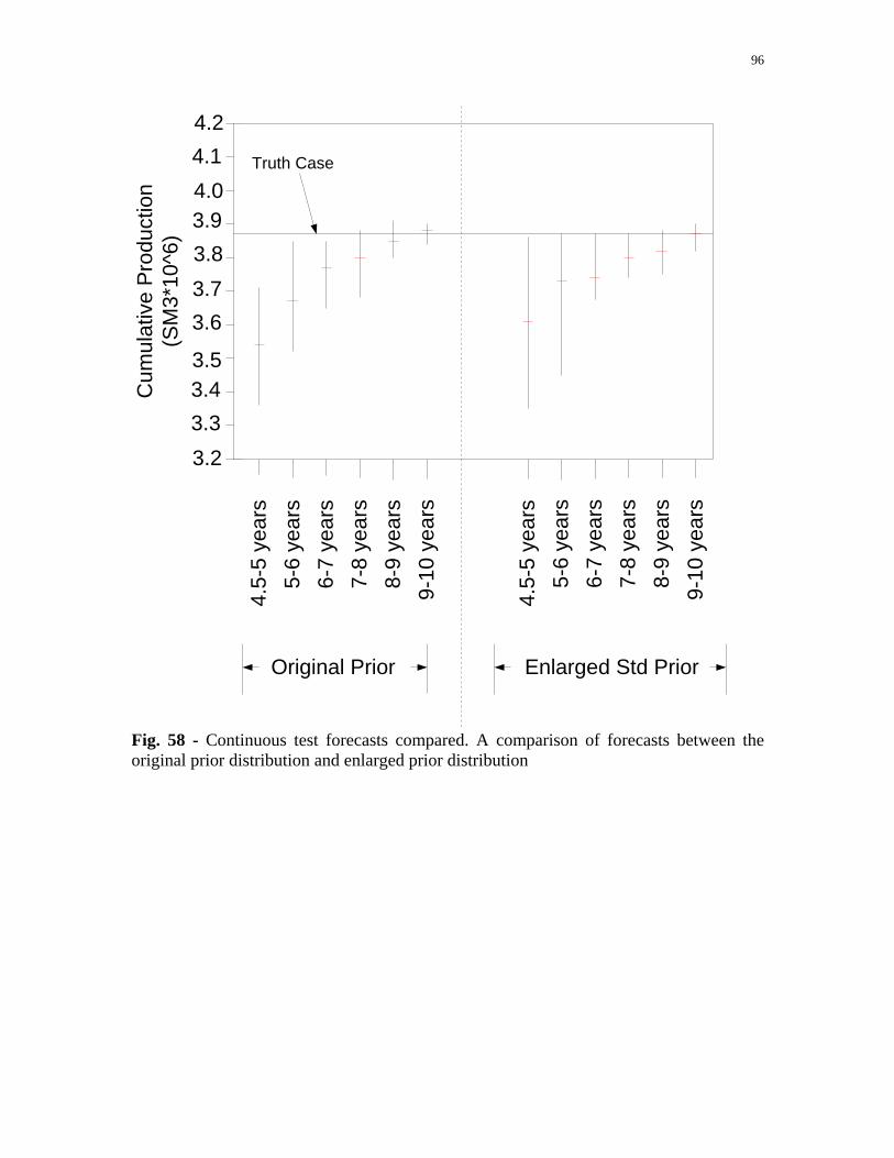
96

3.4 3.3

3.5

3.6 3.73.8

3.9 4.0

4.14.2

3.2

4.5-

5 ye

ars

5-6

year

s6-

7 ye

ars

7-8

year

s8-

9 ye

ars

9-10

yea

rs

4.5-

5 ye

ars

5-6

year

s6-

7 ye

ars

7-8

year

s8-

9 ye

ars

9-10

yea

rs

Truth CaseC

umul

ativ

e P

rodu

ctio

n (S

M3*

10^6

)

Original Prior Enlarged Std Prior

Fig. 58 - Continuous test forecasts compared. A comparison of forecasts between the original prior distribution and enlarged prior distribution

97

Summary of Results

By history matching continuously over the life of a reservoir, we see the uncertainty

range narrowing with time and increased observation data. Compared to the static case,

the continuous approach allows us to generate a reasonable forecast in a much shorter

time (fewer models). This advantage should also allow us to consider more uncertain

parameters in our parameterization, which should result in more reliable forecasts. In

addition, in order to avoid the biased forecasts made in the early years, the continuous

simulation approach provides a way of calibrating uncertainty estimates over time.

98

CONCLUSIONS AND RECOMMENDATIONS

Conclusions

The MCMC method is a strong tool for history matching and quantifying uncertainty. To

the best of my knowledge, the work presented here is the first implementation of this

continuous MCMC history matching process. We can draw the following conclusions

from the tests described above:

1. The static study was consistent with the truth case in forecasts and consistent with

results presented in the literature, demonstrating that a proper initial model and prior

distribution were used. The uncertainty ranges narrow over time, as more information

leads to less uncertainty. In addition, the test shows that we can make improvements

to our assessments of reservoir properties.

2. The continuous study indicates that we can shorten the time to make a reasonable

forecast compared to our static case, by continuing the chain with models that include

more history information as new data are added over time. The continuous approach

allows a more thorough exploration of the parameter than the static case by reducing

the burn-in time of the MCMC process.

3. In the continuous case, the uncertainty ranges shift in addition to narrowing as time

progresses. The continuous simulation approach provides a mechanism for calibrating

uncertainty estimates over time. If it is observed that posterior distributions generated

over time shift in addition to narrowing, then we can either enlarge the standard

deviation of our prior distribution or our observed data to increase the uncertainty.

99

Adjustments should be made until subsequent posterior distributions are bracketed by

all previous distributions.

Recommendations for Future Work

In conducting this study, several additional areas for future work were identified:

1. In my research, the tests were carried out on a synthetic model (PUNQ-S3). Even

though the results demonstrate the benefit of a continuous simulation approach, it

would be helpful to test this method on a live field.

2. Based on the numerous sampled models, it would be useful to withdraw a small set

number of diverse models which represent the posterior distribution reasonably well.

These models could then be used to generate probabilistic forecasts for other

reservoir management decisions (for instance, where and when to drill a new well).

3. In this study, we used the random walk method to get the next sampling candidate.

This method could be replaced by other improved methods which may generate a

better set of samples, especially when the target distribution is multi-modal.

4. Making simulation runs continuously produces a large quantity of output data.

Techniques for storing and managing this data will be necessary in order to run this

process for long periods of time in actual field applications.

100

NOMENCLATURE

obsd = Observed data

m = Uncertain parameters

μ = Prior mean

( )mP = Prior probability distribution

( )mdP obs = Likelihood function

( )obsdmP = Posterior distribution

( )mg = Simulated reservoir response

mC = Parameter covariance matrix

DC = Data covariance matrix

( )mπ = Distribution function

nm = Uncertainty parameters value at state n

( )nmmq = Proposal distribution

R = Acceptance ratio

L = Likelihood function calcy = Calculated data from the simulator obsy = Observed data

c = Constant factor

( )mO = Objective function

vk = Vertical permeability

hk = Horizontal permeability

φ = Porosity

'φ = Porosity value of base map

Kklogμ = Mean of log-normal horizontal permeability

Kklogσ = Standard deviation of log-normal horizontal permeability

101

φX = Uncertainty multiplier of porosity

kX = Uncertainty multiplier of permeability

KXlogμ = Prior mean of log-normal permeability multiplier

kXlogσ = Prior standard deviation of log normal permeability multiplier

( )XP = Prior multiplier distribution

xC = Prior multiplier covariance matrix

φμX = Prior mean of normal porosity multiplier

φσ X = Prior standard deviation of normal porosity multiplier

iσ = Standard deviation of observed data

( )XdP obs = Likelihood function of multiplier

( )obsdXP = Posterior distribution of multiplier

( )XO = Objective function of multiplier

it = State i

1+it = State 1+i

ε = 90-dimensional standard normal random variable

σ = Scale factor

102

REFERENCES

Barker, J.W., Cuypers, M. and Holden, L. 2001. Quantifying Uncertainty in Production Forecasts: Another Look at the PUNQ-S3 Problem. SPE Journal 6 (4): 433-441. SPE-74707-PA.

Bianco, A., Cominelli, A., Dovera, L., Naevdal, G. and Valles, B. 2007. History

Matching and Production Forecast Uncertainty by Means of the Ensemble Kalman Filter: A Real Field Application. Paper SPE 107161 presented at the EUROPEC/EAGE Conference and Exhibition, London, U.K., 11-14 June.

Bos,C.F.M. et al. 1999. Production Forecasting with Uncertainty Quantification (PUNQ).

Final report, Contract No. NITG 99-225 A (December). Capen, E.C. 1976. The Difficulty of Assessing Uncertainty. JPT 28 (8):843-850.

SPE-5579. Craig, David P., Eberhard, Mike J. and Odegard, Chad E. 2005. Permeability, Pore

Pressure, and Leakoff-Type Distributions in Rocky Mountain Basins. SPE Production & Facilities 20 (1): 48-59.

Devegowda, Deepak, Arroyo-Negrete, Elkin, Datta-Gupta, Akhil and Douma, S.G. 2007.

Efficient and Robust Reservoir Model Updating Using Ensemble Kalman Filter With Sensitivity-Based Covariance Localization. Paper SPE 106144 presented at the SPE Reservoir Simulation Symposium, Houston, Texas, 26-28 February.

Floris, F.J.T., Bush, M.D., Cuypers, M., Roggero, F. and Syversveen, A-R. 2001.

Methods for Quantifying the Uncertainty of production Forecasts: A comparative Study. Petroleum Geoscience 7: 87-96.

Gelman, Andrew and Rubin, Donald B. 1992. Inference from iterative simulation using

multiple sequences(with discussion). Statistical Science 7 (4):457-472. Givens, Geof H. and Hoeting, Jennifer Ann 2005. Computational Statistics. New Jersey:

John Wiley & Sons Inc. Goldberg, D.E. 1989. Genetic Algorithms in Search, Optimization, and Machine

Learning. New York city: Addison-Wesley Publishing Co. Greenberg, E. and Chib, S. 1995. Understanding the Metropolis-Hastings algorithm. The

American Statistican 49 (4): 327-335. Gu, Yaqing and Oliver, Dean S. 2004. History Matching of the PUNQ-S3 Reservoir

Model Using the Ensemble Kalman Filter. Paper SPE 89942 presented at the SPE Annual Technical Conference and Exhibition, Houston, Texas, 26-29 September.

103

Hastings, W. K. 1970. Monte Carlo Sampling Methods Using Markov Chains and Their

Applications. Biometrika 57 (1): 97-109. Holden, L. 1998. Adaptive chains. Technical Report. Norwegian Computing Center

(November 1998). Holmes, Jay C., McVay, Duane A. and Senel, O. 2007. A System for Continuous

Reservoir Simulation Model Updating and Forecasting. Paper SPE 107566 presented at the Digital Energy Conference and Exhibition, Houston, Texas, 11-12 April.

Howard, R.A. 2005. Decision Analysis, class notes, Department of Management Science

and Engineering, Stanford University, Stanford,CA. Liu, Ning and Oliver,Dean S. 2003. Evaluation of Monte Carlo Methods for Assessing

Uncertainty. SPE Journal 8 (2): 188-195. SPE- 84936. Ma, X., Al-Harbi, M., Datta-Gupta, Akhil and Efendiev, Y. 2006. A Multistage Sampling

Method for Rapid Quantification of Uncertainty in History Matching Geological Models. Paper SPE 102476 presented at the SPE Annual Technical Conference and Exhibition, San Antonio, Texas, 24-27 September.

Nævdal, Geir, Johnsen, Liv Merethe, Aanonsen, Sigurd Ivar, Hydro, Norsk and Vefring,

Erlend H. 2003. Reservoir Monitoring and Continuous Model Updating Using Ensemble Kalman Filter. Paper SPE 84372 presented at the SPE Annual Technical Conference and Exhibition, Denver, Colorado, 5-8 October.

Thakur, G.C. 1996. What is reservoir management? JPT 48 (6):520-525. Thomas, G.W. 1986. The Role of Reservoir Simulation in Optimal Reservoir

Management. Paper SPE 14129 presented at the SPE International Meeting on Petroleum Engineering, Beijing, 17-20 March.

Vose, D. 2000. Risk Analysis: A Quantitative Guide. Second edition, New York city:

John Wiley&Sons Inc.

104

VITA

Name: Chang Liu

Address: Harold Vance Department of Petroleum Engineering 3116 TAMU, College Station, TX 77843-3116 Email Address: [email protected] Education: B.A., Applied Mathematics, Peking University, 2006 M.S., Petroleum Engineering, Texas A&M University, 2008

continuous reservoir simulation model updating and - CORE

Documents

Transcript of continuous reservoir simulation model updating and - CORE