Proceedings of the XXVI Iberian Latin-American Congress on Computational Methods in Engineering CILAMCE 2005Brazilian Assoc. for Comp. Mechanics & Latin American Assoc. of Comp. Methods in EngineeringGuarapari, Espırito Santo, Brazil, 19th–21st October 2005

Paper CIL0620

ANALYSIS OF TRANSIENT LOADS ON CABLE-REINFORCED CONVEYORBELTS WITH DAMPING CONSIDERATION

R. PascualV. Meruanerpascual@ing.uchile.clvmeruane@ing.uchile.clMechanical Engineering Department, Universidad de Chile, Beauchef 850, Santiago, Chile

G. Barrientosgbarrien@udec.clMechanical Engineering Department, Universidad de Concepcion, Concepcion, Chile

Abstract. This work presents a methodology to compute dynamic stress distributions onlarge conveyor belts considering a viscous-damping model. Results could be very usefulat the conveyor design stage since at starts and stops of the system, large dynamic loadsmay be encountered. Such loads may produce a catastrophic failure of the conveyor, withimportant direct and downtime costs. We present a finite- element based methodology anduse the Newmark time-integration method to solve the transient responses. Our schemeincludes the effects of damping. A real-life industrial case is analyzed and three criticalsituations are considered: normal stop, sudden stop, suddenly aborted start. Results areshown in terms of dynamic loads at critical points of the system. The simulations showthat the damping effects are negligible in the analysis of real-life designs, thus allowingthe use of the analytical solution. For the analized case, maximum loads obtained withthe present methodology are smaller in 5% than those obtained with the conservativeapproach.

Keywords:Structural dynamics, large conveyor belts, finite element, transient analysis.

1. INTRODUCTION

A large variety of industries use large conveyor belts to move raw material betweenprocess units. Recent technology has been developed to meet the industry needs, leadingto systems with improved mechanical properties, increased strength and wear properties,and other specific properties associated to each application. Conveyor belts are also ofgreat use in the mining industry. There, designs consider the use of steel-cable reinforcedbelts in order to support the large static and dynamic loads that appear. At the design stage,it is very important to estimate the dynamic loads that a conveyor belt may suffer in orderto specify system dimensions and material selection. There exists a tradeoff between theinvestment in an oversized belt and the downtime cost associated to a catastrophic failureof an undersized belt. Traditional design standards for belt conveyor with less than 1000m. References (1)-(2) do not consider explicitly the elastic characteristics of the belt.They are based on empirical data from conveyors of medium length, with no input fromcurrent large distance (up to several kilometers) applications.

CILAMCE 2005 – ABMEC & AMC, Guarapari, Espırito Santo, Brazil, 19th – 21st October 2005

The situation may be modelled using the one-dimensional wave equation, whosesolution is well known when the initial velocity conditions are given. When, as in thecase of conveyor belts, initial conditions are given in terms of acceleration, obtaining ananalytical solution is much more complex. Previous works only deal with conservativesystems (3).

Harrison (4; 5; 6) establishes an analytical solution to the problem by modelling interms of stress waves that propagate in time trough the belt, and quantifies the dynamicstress. His model is one-dimensional which does not permit the analysis of other loadslike shear loads and torsion loads.

The objective of this work is to evaluate the effect of damping on the dynamic re-sponses of a large-scale conveyor belt. By doing so, we will be able to understand howdamping may be used to control and reduce the dynamic stress under transient load situ-ations.

Wheeler (7) presents a method to calculate the flexure resistance at the design stage,with the view of minimising these resistances to improve the efficiency of the belt. Platetheory is used to approximate the deflection of the troughed conveyor belt between idlersets. In reference (8), Wheeler analyzes the rotating resistance of belt conveyor idler rollsoccurs due to the friction of the rolling elements in the bearings, the viscous drag of thelubricant and the friction of the contact lip seals. He presents models to estimate therotating resistance of idler rolls and discuss an apparatus designed to measure the rotatingresistance under simulated operating conditions.

2. ANALYTICAL MODEL

Figures 1 and 2 show a typical configuration of an industrial conveyor belt. It iscomposed of a belt, a drive pulley that provides the necessary driving torque; a drivenpulley; rollers to support the belt; and a system to keep the tension which may be a tailmass or a spring system. Under nominal conditions, the belt is loaded on the upper sideand unloaded on the lower side. During starting and stopping of a conveyor system, largestress are on the belt caused by the motor pulley. On one side, we observe traction andcompression waves. Low frequency oscillations are also seen at the tail pulley and at thetail mass(3). Experience shows that the vibration frequency induced on the tail pulley andthe tail mass is about 10 times smaller compared to the frequency of the elastic wave, sowe may consider negligible the first effect with respect to the second (3).

Harrison (3) argues that the propagation velocity of the elastic wave determines thedynamic tension of the belt. For a cable-reinforced belt, such velocity is given by:

vsc =

√Esc

ρsc

=

√EscAsc

µsc

(1)

whereµsc is the mass of the steel cable per unit length andAsc corresponds to its crosssection. If the cables are covered by an elastomeric layer, there exists a delaying effectdue to the mass of the rubber (experimentally verified by Harrison(4)). The rollers andthe raw material also delay the propagation of the wave. In order to consider these effects,we define an equivalent mass per unit length:

µeq = µb + µil + µl (2)

CILAMCE 2005 – ABMEC & AMC, Guarapari, Espırito Santo, Brazil, 19th – 21st October 2005

0

Figure 1: Basic scheme of a conveying system

ANEXO A Análisis experimental. Para obtener las propiedades mecánicas de la correa, se llevan a cabo dos pruebas experimentales en un trozo representativo de una correa transportadora real. Para poder sacar conclusiones sobre las pruebas que se realizan, se debe suponer que el trozo de prueba de que se dispones es representativo de una correa homogénea y que se mantienen las propiedades que se desean evaluar inalteradas, osea es válida la estimación de cualquier parámetro de la correa mediante las estadísticas obtenidas en la muestra. Esta muestra es de tamaño 40x28 cm2 y 3 cm de espesor, fabricada de caucho y reforzada por cables de acero, de 8 mm de diámetro, como se aprecia en la figura 2, cuya masa es de 5.194 Kg, siendo su densidad de 32.46 Kg/m2.

Figura 2

Determinación del coeficiente de amortiguamiento “c”. El primer parámetro que se estima es el coeficiente de amortiguamiento de la correa, para esto se sigue el siguiente procedimiento: -Se realiza un ensayo de golpe sobre la correa montada como se muestra en la figura 3, de manera de generar vibraciones libres en el material. Como la correa se trata de un material compuesto, se toman varias mediciones, dándole los golpes que fuerzan la vibración en ambos materiales, esto es, tanto sobre el caucho como sobre los cables de acero que la refuerzan. Además se hace vibrar longitudinalmente, que es la dirección que interesa par el presente trabajo.

Figure 2: Belt cross section

CILAMCE 2005 – ABMEC & AMC, Guarapari, Espırito Santo, Brazil, 19th – 21st October 2005

whereµb is the belt mass per unit length,µil is an equivalent rollers’ mass per unit length,µl corresponds to the raw material mass per unit length. The equivalent density of theloaded belt is then:

ρb =µeq

Asc

(3)

and the velocity of the wave is estimated as:

vcl =

√Eb

ρb

=

√Esc

ρsc

ρsc

ρb

= vsc

√ρsc

ρb

= vsc

õsc

µeq

(4)

Equation (4) assumes that the material is uniformly distributed along the belt, with norelative movement between the raw material and the belt.vcl represents to a lower boundfor the wave propagation velocity. If the conveyor is unloaded:

vcl = vsc

õsc

µb + µil

(5)

We also must consider that the wave front has different velocities in each side of theconveyor. For the return side, we have:

vr = vsc

õsc

µb + µir

(6)

whereµir is the mass per unit length on the return side.In real-life applications, belts work partially loaded and load adhesion depends on

the nature of the raw material. For these reasons, Harrison (5) proposes a correction tovelocityvc given by:

vc = vcu − αq

q0

(vcu − vcl) (7)

whereα is the coupling factor between the raw material and the belt. He considers 0.8 forgranulated material and humid material, and0.3 for rocks (diameter0.2 m). If we considerahomogeneousbelt model, there will be a single wave propagation speed velocity, whichcorresponds to the average value:

v0 =vr + vc

2(8)

Once we have estimated the velocity at which the wave front advances, we mayevaluate the time interval needed for it to go trough the belt. If we consider constantvelocity propagation, it takes:

Tc =l

2

1

vc

time units to go trough the load side of the belt when it is unloaded.l correspondes to thebelt length. When it is loaded it takes:

Tcl =l

2

1

vcl

CILAMCE 2005 – ABMEC & AMC, Guarapari, Espırito Santo, Brazil, 19th – 21st October 2005

time units. We also know that it takes

Tr =l

2

1

vr

time units to return to the driven pulley.The cycle interval when the belt loaded and unloaded respectively:

Tl = Tcl + Tr

Tu = Tc + Tr

We may also define the propagation interval as:

τ =2l

v0

(9)

According to wave theory (14), the maximum dynamic load occurs at the origin (seefigure 3) and at the instant:

tf max =τ

2=

l

v0

(10)

2.1 System inertias

The mass of the rotating parts (pulleys, gears, couplings) are considered as an equiv-alent mass in traslation, which has the same amount of kinetic energy as the rotatingsystem:

Tsr =1

2

[Imnmω2

m + Igngω2g + Icncω

2c

](11)

wherenm is the number of motors, with a moment of inertiaIm, ng is the number of gears,with a moment of inertiaIg, nc is the number of couplings, with a moment of inertiaIc,andωi is the angular velocity of the componenti.

The equivalent traslation kinetic energy of the rotative parts is:

T =1

2m1v

2b (12)

Using (11) and (12) we obtain:

m1 =1

v2b

[Imnmω2

m + Igngω2g + Icncω

2c

](13)

The mass of the driving pulleym2 and from the driven pulleym3 are computed using thesame scheme. In order to compute the energy at the rollers, we use their mass on bothsides of the belt (µil andµr). The length of both sides is the same so we may define:

m4 =l

2(µr + µil) (14)

CILAMCE 2005 – ABMEC & AMC, Guarapari, Espırito Santo, Brazil, 19th – 21st October 2005

For the belt, we compute its equivalent mass fromµb and define:

m5 = µbl (15)

For the raw material we use:

m6 = µll

2(16)

Now, we are in position to estimate the total mass of the system as:

meq =5∑

i=1

mi + α0m6 (17)

whereα0 correspond to the fraction of the nominal load capacity being transported.Equation (17) corresponds to the mass in movement; nevertheless it does not repre-

sent the mass that effectively transmits the wave front. For that we consider:

mef = meq −m1 −m2 (18)

which allow us to estimate the effective average mass per unit length:

µef =mef

l(19)

2.2 Belt loads

In stationary regime, the belt is subjected to static loadsf1 andf2, respectively. Intransient situations, we need to add the dynamic loadsfd. On the lower side and uppersides of the belt respectively:

fr = f2 + fd (20)

fc = f1 + fd (21)

Harrison (1) determinesmax(fd) using the method of impedance:

max(fd) = mefv0∂u

∂t max(22)

whereu is the axial displacement.

3. NUMERICAL MODEL

The model for the belt is based on the work of Harrison (14). It assumes the belt asa bar clamped on both extremes to a moving rigid structure, as it is shown in figure 3.The bar has lengthl. The system has an initial traslation velocity (i.e., nominal conveyoroperation), which may also be cero (starting). PointsA andB do not have relative motionwith respect to the reference structure.

Existing analytical solutions consider conservative systems where the mass is uni-formly distributed along the belt; as a consequence, it is there assumed constant propa-gation velocity on both load and discharge parts of the belt. On the other hand, the useof a finite elements model allows us to model variable mass distribution and damping. Insuch a way, we take into account that the upper part of the belt carries raw material, whilethe lower part does not. These arguments justify the use of numerical solutions to theproblem.

CILAMCE 2005 – ABMEC & AMC, Guarapari, Espırito Santo, Brazil, 19th – 21st October 2005

0

Figure 3: Mathematical model of the belt

3.1 Finite elements model

Following the finite elements method (9), we discretize the belt inton bar elements,each connected to the next trough a node. For this kind of element, the displacement fieldis approximated with a first order polinomial. The element stiffness and mass matricesare given by:

Ke =EA

le

[1 −1−1 1

](23)

Me =ρAle

2

[1 −1−1 1

](24)

whereE is the Young modulus,A is the cross section of the element,ρ is the massper unit volume. We also assume that movement is exclusively axial.

The elementary damping matrixCe is built considering a single viscous damper withconstantc:

Ce = c

[1 −1−1 1

](25)

After discretization, we solve the matrix equation:

Mx + Cx + Kx = f (26)

wheref is the vector that describes the external loads,M is the mass matrix,C is thedamping matrix,K is the stiffness matrix andx is the displacement vector. In order tosolve (26) we use the Newmark method (9).

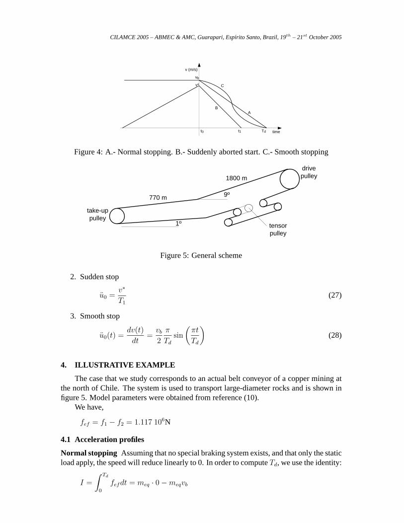
We simulated for three transient situations, as it is shown in figure 4:

1. Normal stop

u0 =vb

Td

CILAMCE 2005 – ABMEC & AMC, Guarapari, Espırito Santo, Brazil, 19th – 21st October 2005

B

C

A

time

v (m/s)

t0 t1 Td

v*

vb

Figure 4: A.- Normal stopping. B.- Suddenly aborted start. C.- Smooth stopping

1º

9º

tensor pulley

drive pulley

take-up pulley

770 m

1800 m

Figure 5: General scheme

2. Sudden stop

u0 =v∗

T1

(27)

3. Smooth stop

u0(t) =dv(t)

dt=

vb

2

π

Td

sin

(πt

Td

)(28)

4. ILLUSTRATIVE EXAMPLE

The case that we study corresponds to an actual belt conveyor of a copper mining atthe north of Chile. The system is used to transport large-diameter rocks and is shown infigure 5. Model parameters were obtained from reference (10).

We have,

fef = f1 − f2 = 1.117 106N

4.1 Acceleration profiles

Normal stopping Assuming that no special braking system exists, and that only the staticload apply, the speed will reduce linearly to 0. In order to computeTd, we use the identity:

I =

∫ Td

0

fefdt = meq · 0−meqvb

CILAMCE 2005 – ABMEC & AMC, Guarapari, Espırito Santo, Brazil, 19th – 21st October 2005

Definition Symbol Value UnitNominal belt speed vb 4.75 m/sbelt half length l/2 2561 mbelt mass per unit length µb 118 kg/mcable mass per unit length µsc 53 kg/mraw material mass per unit length µl 287 kg/mrollers mass per unit length (upper side)µil 67 kg/mrollers mass per unit length (lower side)µir 20 kg/mBelt nominal capacity q0 4.92 106 Kg/hDriving pulley mass 27.3 103 kgOther masses 45.5 103 kgMotor inertia Im 150 kgm2

Gears inertia Ig 10 kgm2

Coupling inertia Ic 10 kgm2

Static load f1 1.417 106 NStatic load f2 0.300 106 NMotors nm 4Gears ng 4Couplings nc 4

Table 1: Model parameters

Element Symbol Value (103 Kg)Drive pulley m2 27.3Driven pulley m3 45.0Rollers m4 222.8Belt m5 604.4Raw material m6 735.0

Table 2: System Inertias

then,

Td =mevb

fef

(29)

From equation (13) we have:

m1 = 359.7 103Kg

The rest of mass parameters is detailed in table (2).So the total mass is:

me =∑

i

mi = 1994.7 103Kg

and

Td =mevb

Te

=1994.7

1117.04.75 = 8.5 s

CILAMCE 2005 – ABMEC & AMC, Guarapari, Espırito Santo, Brazil, 19th – 21st October 2005

v (m/s)

v*

T0 T1

B

t0 t1

time

⎟⎟⎠

⎞⎜⎜⎝

⎛+⎟⎟

⎠

⎞⎜⎜⎝

⎛

1

*

0

*

arctanarctanTv

Tv

Figure 6: Aborted start. Speed of drive pulley vs time.

From which we may compute the constant negative acceleration to be used duringthe integration:

q =−4.75

8.5= −0.5588 m/s2

Suddenly aborted start An aborted start corresponds to a sudden stop of the systemwhen it starts to accelerate to find its nominal speed (i.e., due to an overload trip). Accord-ing to Harrison(10), the sudden change in the acceleration pattern induces an impulsiveeffect on the belt, which takes it to a speed:

v∗∗ = T1 tan

[arctan

(v∗

T0

)+ arctan

(v∗

T1

)](30)

which generates a dynamic load (see figure 6). We assume that there exists an accel-eration betweent0 y t0 + t1:

qa = −v∗∗

T1

From the data:

v∗∗ = 4.44 m/s

qa = −4.44

6.8m/s2

Smooth stopping We consider a system where acceleration follows a sine function intime (figure 4) and its given by equation (28). In such a way, no discontinuities appear inthe acceleration. In our case:

u0(t) =4.75

2

π

8.5sin

(πt

8.5

)

CILAMCE 2005 – ABMEC & AMC, Guarapari, Espırito Santo, Brazil, 19th – 21st October 2005

Figura *

-Sobre el material se ubica un sensor de vibraciones, de tipo acelerómetro; que entrega como respuesta 100 mV/g (g: aceleración de gravedad). Este sensor es fijado mediante cera, por lo que se pueden tomar mediciones desde prácticamente cero Hertz hasta un límite máximo de 32 KHz, que corresponde a una fijación con espárrago, por lo que en la práctica no se alcanza ese valor; pero para el rango requerido no tiene mayor implicancia. -El sensor esta conectado a un analizador de vibraciones “Spectral Dynamics SD380 Signal Analizer”, marca Scientific Atlanta, que se ve en la figura *

Figura 4

Figure 7: Damping identification setup

The equivalent stiffness is estimated from the effective mass per unit length and thepropagation velocity:

k = µefv20 (31)

We also assume a constant propagation velocityv0:

v0 = 2355 m/s

The stiffness of the belt is:

k = 1.74 109 N

For the numerical integration we use the Newmark method with integration parame-tersβ = 1

4andγ = 1

2. These values assure a robust convergence. In what follows, we

show the results for the different cases of study. We first perform an analysis with nodamping, an then we compare results using feasible damping values.

4.2 Damping identification

Figure 7 shows the experimental setup used to estimate the damping factor for thefirst mode shape (elongation mode). The belt is in a free-free border condition and aninitial displacement condition. Assuming that the transient response was dominated bythe first mode shape, we obtained an estimation ofξ1 = 0.06, which is the expected rangefor this kind of material (15).

4.3 Results

Conservative systemWe show results for the aborted start case. The belt conveyor startsto increase to its nominal speed and when it reaches 80% the belt stops suddenly. Accord-ing to Harrison, this can be modelled using a virtual speed of4.44 m/s, so we have theinitial conditions (according to figure 3):

u(x, t) = 4.44 m/s

u(0, t) = −0.6529 m/s2

u(l, t) = −0.6529 m/s2

CILAMCE 2005 – ABMEC & AMC, Guarapari, Espırito Santo, Brazil, 19th – 21st October 2005

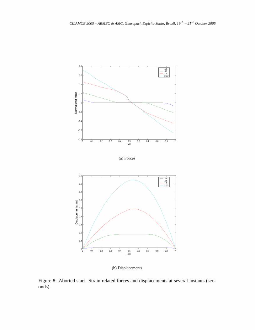
The maximum tension attains a value of1.018 106 N at x = 0, instant2.22 s. Thisvalue is16.8% higher than the one obtained with a normal stop. Figure 8(a) shows thelevel of the dynamic loads for several instants.

Figure 8(b) shows the strain related displacements at several instants. The maximumvalue attains0.86 m att = 2.22 s. We observe asymmetrical responses due to the correc-tion of the mass distribution. Response amplitudes are increased with respect to the casewhere no mass asymmetry is considered.

Damped systemThe stiffness of the belt was estimated from the average effective massof the system as well as with the average wave propagation velocity:

k = µefv20 = 313.8 · 23552 = 1.74 109 N/m (32)

Using this equivalent stiffness and mass parameters we estimate the critical damp-ing from cc = 2

√km. From the experimental damping factorξ = c/cc we obtain an

estimation for the damping parameterc. We have:

k =1.74 109

5122= 339711 N/m

The belt mass is6.044 105 Kg and

cc = 2√

339711 · 604400 Kg/s

ξ = 0.4, and:

c = 3.62 105 Kg/s

We take this value as reference and we used it for the aborted start case. Figure 9 showsthe effect of several damping levels on the maximum load.

We observe that for damping values abovec = 45 104 Kg/s the system shows novibrations and the load profile is similar to the one atx = 0.

5. CONCLUSIONS

This article builds on previous research from Riffo (11), Fuentes (12) and Amigo(13). The work analyzes the effect of non-uniformity in the distribution of mass along thebelt (charge and discharge sides) and also damping effects on transient response due tosuddenly aborted starts and stops. Comparing to previous research, we find a reduction ofonly 4% in maximum reactions, showing that damping effects are negligible. Of course,this result is valid for the configuration in study. To the authors knowledge no previousresults appear in the available literature. The implementation of the method is quite simpleand the strategy shows a lot of flexibility to handle different model parameters and borderand initial conditions.

Acknowledgements

The authors wish to acknowledge the partial financial support of this study by theFOndo Nacional de DEsarrollo Cientifico Y Tecnologico (FONDECYT) of the chileangovernment (projects 1020810 and 1030943).

CILAMCE 2005 – ABMEC & AMC, Guarapari, Espırito Santo, Brazil, 19th – 21st October 2005

0 0.1 0.2 0.3 0.4 0.5 0.6 0.7 0.8 0.9 1-0.8

-0.6

-0.4

-0.2

0

0.2

0.4

0.6

0.8

x/l

Nor

mal

ized

forc

e

.25

.751.52.22

(a) Forces

0 0.1 0.2 0.3 0.4 0.5 0.6 0.7 0.8 0.9 10

0.1

0.2

0.3

0.4

0.5

0.6

0.7

0.8

0.9

x/l

Dis

plac

emen

ts [m

]

.25

.751.52.22

(b) Displacements

Figure 8: Aborted start. Strain related forces and displacements at several instants (sec-onds).

CILAMCE 2005 – ABMEC & AMC, Guarapari, Espırito Santo, Brazil, 19th – 21st October 2005

0 0.1 0.2 0.3 0.4 0.5 0.6 0.7 0.8 0.9 1-0.01

-0.005

0

0.005

0.01

0.015

0.02

0.025

0.03

Normalized time

Nor

mal

ized

forc

e

03 104

105

4.5 105

106

Figure 9: Dynamic load atx = l/2 for several damping levels

REFERENCES

[1] German Industrial Standard, 1982.Belt Conveyers for Bulk Materials, DIN 22101.

[2] CEMA, 1997.Handbook of Belt conveyors for Bulk Materials.

[3] Harrison, A., 1986.Stress front velocity in elastomer belts with bonded steel cablereinforcing, Bulk Solids Handling, 6(1), 27-31.

[4] Harrison, A., 1996.Simulation of conveyor dynamics, Bulk Solids Handling, vol.16, n. 1, pp. 33-36.

[5] Harrison A.,1996.15 Years of conveyor belt nondestructive evaluation, Bulk SolidsHandling, vol. 16 , n. 1, pp. 13-19.

[6] Harrison A., 1998.On the appropriate use of dynamic stress models for conveyordesign, Bulk Solids Handling, vol. 8, n. 6, pp. 677-680.

[7] Wheeler, C.A., Roberts, A.W., Jones, M.G., 2004.Calculating the Flexure Resis-tance of Bulk Solids Transported on Belt Conveyors, Particle & Particle SystemsCharacterization, vol. 21, n. 4, pp. 340-347.

[8] Wheeler, C.A., 2003.Analysis of the Main Resistances of Belt Conveyors, Ph.DThesis, Chapter 5, The University of Newcastle, Australia.

[9] Bathe, K.J., 2003.Finite Element Procedures, Prentice-Hall of India.

CILAMCE 2005 – ABMEC & AMC, Guarapari, Espırito Santo, Brazil, 19th – 21st October 2005

[10] Harrison, A., 1988.Informe tecnico a la empresa Chuquicamata, Chile.

[11] Riffo, F., 2000.Analisis numerico del comportamiento dinamico de una correatransportadora. Thesis, Universidad de Concepcion, Concepcion.

[12] Fuentes J.P., 2002.Modelacion numerica de las fuerzas dinamicas producidas enuna correa transportadora de gran longitud, Thesis, Universidad de Concepcion,2002.

[13] Amigo O., 1990.Analisis dinamico de correas transportadoras, Tesis de Magıster,U. de Concepcion.

[14] Harrison A., 1983.Criteria for minimizing transient stress in conveyor belts, Me-chanics eng. Trans. I.E.Aust., vol. 8, n. 3, pp. 129-134.

[15] Harris, C.M., 1996.Shock and Vibration Handbook, 4th ed., Mc-Graw-Hill.