TRANSIENT ANALYSIS

OF SIX-PHASE SYNCHRONOUS MACHINESby

SAID MOZAFFARI

B.Sc. (Civil E), United States International University, 1987

B.A.Sc. (EE), University of British Columbia, 1990

A MILS'S SUBMITTED IN PARTIAL FULFILLMENT OF

THE REQUIREMENTS FOR 11:it, DEGREE OF

MASTER OF APPLIED SCIENCE

in

Tilt FACULTY OF GRADUATE STUDIES

DEPARTMENT OF ELECTRICAL ENGINEERING

We accept this thesis as conforming

to the required standard

THE UNIVERSITY OF BRITISH COLUMBIA

March 1993

©Said Mozaffari, 1993

In presenting this thesis in partial fulfilment of the requirements for an advanced

degree at the University of British Columbia, I agree that the Library shall make it

freely available for reference and study. I further agree that permission for extensive

copying of this thesis for scholarly purposes may be granted by the head of my

department or by his or her representatives. It is understood that copying or

publication of this thesis for financial gain shall not be allowed without my written

permission.

(Signature)

Department of E6C-17 L•CcIt

The University of British ColumbiaVancouver, Canada

Date 1-fai"ch e3, ict1.5

DE-6 (2/88)

ABSTRACT

Six-phase synchronous machines have been used in the past for high power generation, and

presently are being used in high power electric drives and in ac and/or dc power supplies. This

thesis presents a mathematical model for investigating the transient performance of a six-phase

synchronous machine, and develops a model for the simulation of such machines with the EMTP.

The effect of the mutual leakage coupling between the two sets of three-phase stator windings are

included in the development of a d-q equivalent circuit. The six-phase machine is constructed

from a three-phase machine by splitting the stator windings into two equal three-phase sets. The

six-phase machine reactances and resistances are derived by relating their values to the known

three-phase machine values. The transient performance of the machine is tested by solving the

machine equations for a case of a six-phase short-circuit at the terminals of the machine. The

EMTP model presented is based on representing the six-phase machine as two three-phase

machines in parallel. The EMTP model verification is achieved by comparing the EMTP results

against an independent computer program, for the case of a six-phase short-circuit test at the

terminals of the machine.

ii

TABLE OF CONTENTS

Abstract^ ii

List of Tables

List of Figures^ vi

Acknowledgement^ vii

Dedication^ viii

1. INTRODUCTION 1

1.1 History of Six-Phase Synchronous Machines 1

1.2 Objective of the Thesis 2

2. EQUIVALENT CIRCUIT OF A SIX-PHASE 4SYNCHRONOUS MACHINE

2.1 Introduction 4

2.2 Differential Equations 5

2.3 Stator Mutual Leakage Inductances 9

2.4 Flux Equations 9

2.5 Transformation of the Machine Equations 11

2.6 Equivalent Circuit of the System 14

3. SIX-PHASE MACHINE PARAMETERS 17

3.1 Introduction 17

3.2 Synchronous Self-Reactance of a Three-Phase Machine 17

3.3 Stator Leakage Reactance of a Three-Phase Machine 17

iii

3.4^Relating Six-Phase Machine Parameters to a Three-Phase Machine^19

3.5^Stator Leakage Reactance of a Six-Phase Machine^21

3.6^Machine Parameters^ 23

4. TRANSIENT ANALYSIS^ 27

4.1^Introduction^ 27

4.2^Symmetrical Short-Circuit of a Unloaded Six-Phase Synchronous Machine 27

4.3^Solution of the Differential Equation^ 29

5. EMTP MODEL FOR THE SIX-PHASE^ 35SYNCHRONOUS MACHINE

5.1^Introduction^ 35

5.2^Model of the Machine^ 35

5.3^Method of Current Injection^ 39

5.4^Numerical Instability Caused by Time Delays^ 42

5.5^Testing the EMTP Model^ 44

6.^CONCLUSIONS^ 47

6.1^Results in Thesis^ 47

6.2^Suggestion for Future Work^ 48

REFERENCES^ 50

APPENDIX A^ 52

APPENDIX B^ 57

APPENDIX C^ 59

iv

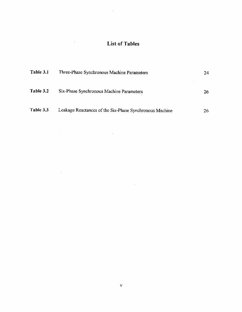
List of Tables

Table 3.1^Three-Phase Synchronous Machine Parameters^ 24

Table 3.2^Six-Phase Synchronous Machine Parameters^ 26

Table 3.3^Leakage Reactances of the Six-Phase Synchronous Machine^26

v

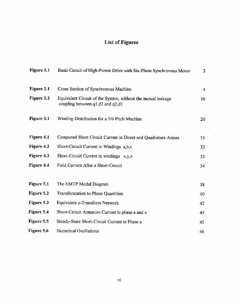
List of Figures

Figure 1.1^Basic Circuit of High-Power Drive with Six-Phase Synchronous Motor^2

Figure 2.1^Cross Section of Synchronous Machine^ 4

Figure 2.2^Equivalent Circuit of the System, without the mutual leakage^16coupling between ql,d2 and q2,d1

Figure 3.1^Winding Distribution for a 5/6 Pitch Machine^ 20

Figure 4.1^Computed Short Circuit Current in Direct and Quadrature Axises^31

Figure 4.2^Short-Circuit Current in Windings a,b,c^ 32

Figure 4.3^Short-Circuit Current in windings x,y,z^ 33

Figure 4.4^Field Current After a Short-Circuit^ 34

Figure 5.1 The EMTP Model Diagram^ 38

Figure 5.2^Transformation to Phase Quantities^ 40

Figure 5.3^Equivalent z-Transform Network^ 42

Figure 5.4^Short-Circuit Armature Current in phase a and x^ 45

Figure 5.5^Steady-State Short-Circuit Current in Phase a^ 45

Figure 5.6^Numerical Oscillations^ 46

vi

ACKNOWLEDGEMENT

I would like to thank my wife Suzanne Belanger for her moral support and constant

encouragement. I send my regards to my parents for their love, nurturing and support.

I am indebted to my supervisor, Dr. H.W. Dommel, for his constant guidance and his

indispensable role in the successful completion of this thesis. I express my gratitude to Dr. M.

Wvong and Dr. L.M. Wedepohl , for their careful examination of this thesis.

I would also like to thank my good friends and fellow students in the Power Group of the

Electrical Engineering Department at U.B.C, for their dedication to providing a friendly and

cooperative environment for research. In particular, I like to thank A. Araujo, and Dr. N.

Santiago for providing me with helpful comments and suggestions.

vii

DEDICATION

I would like to dedicate this work to my father Mohammad Hossein Mozaffari.

viii

Chapter 1

INTRODUCTION

1.1 History of Six-Phase Synchronous Machines

In the late 1920's, the drive toward building larger generating units was hampered by

limitations in circuit breaker interrupting capacity and by the large size of reactors needed to limit

the fault currents. To overcome this problem, six-phase synchronous machines were built with

two sets of three-phase windings [1], in which each set of three-phase stator windings was

connected to its own station bus. The voltages of each set were equal and in phase. Such

generators, rated up to 175 MVA, were in use until the fault current problem was solved by

connecting each generator to its own step-up transformer, with switching accomplished on the

high voltage side where the currents are lower.

During the last few years, six-phase synchronous motors have been used in high power

electric drives. In these inverter-fed synchronous motors, each of the three-phase stator winding

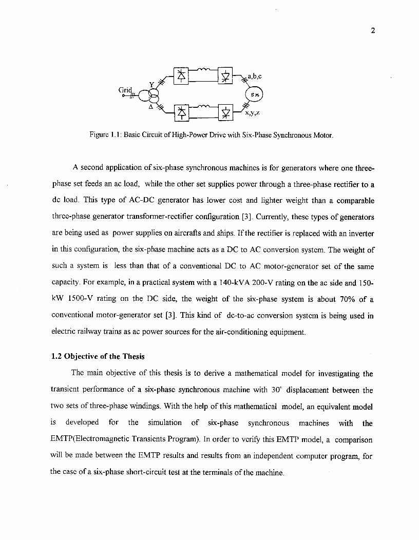
sets is connected to its own inverter. Figure 1.1 shows the basic circuit diagram of such a twelve-

pulse inverter-fed synchronous motor with two three-phase windings. This circuit configuration is

very beneficial for the reduction of harmonic losses and torque pulsations if the two sets of

windings are displaced by 30° [2]. On the supply side, which consists of two bridge rectifiers fed

by a three-winding transformer with Yz\ connection, giving a line shift of 30°, the 5th and 7th

harmonic are canceled out. The two machine-side inverters each feed a set of three-phase

windings of the machine. The two three-phase sets are displaced by 30° and cancel out the field

caused by the 5th and 7th harmonics of the stator winding currents.

1

2

Figure 1.1: Basic Circuit of High-Power Drive with Six-Phase Synchronous Motor.

A second application of six-phase synchronous machines is for generators where one three-

phase set feeds an ac load, while the other set supplies power through a three-phase rectifier to a

dc load. This type of AC-DC generator has lower cost and lighter weight than a comparable

three-phase generator transformer-rectifier configuration [3]. Currently, these types of generators

are being used as power supplies on aircrafts and ships. If the rectifier is replaced with an inverter

in this configuration, the six-phase machine acts as a DC to AC conversion system. The weight of

such a system is less than that of a conventional DC to AC motor-generator set of the same

capacity. For example, in a practical system with a 140-kVA 200-V rating on the ac side and 150-

kW 1500-V rating on the DC side, the weight of the six-phase system is about 70% of a

conventional motor-generator set [3]. This kind of dc-to-ac conversion system is being used in

electric railway trains as ac power sources for the air-conditioning equipment.

1.2 Objective of the Thesis

The main objective of this thesis is to derive a mathematical model for investigating the

transient performance of a six-phase synchronous machine with 30° displacement between the

two sets of three-phase windings. With the help of this mathematical model, an equivalent model

is developed for the simulation of six-phase synchronous machines with the

EMTP(Electromagnetic Transients Program). In order to verify this EMTP model, a comparison

will be made between the EMTP results and results from an independent computer program, for

the case of a six-phase short-circuit test at the terminals of the machine.

3

In Chapter 2, the differential equations of a six-phase synchronous machine are first derived

in phase variables. Park's transformation [4] will then be used to transform the machine equations

to the d-q-O rotor reference frame. This model includes the stator mutual leakage reactances [5],

which have been ignored in earlier works [6,7].

Chapter 3 describes the calculation of the six-phase self and mutual reactances and

resistances, which are needed for the simulation of transient phenomena. The six-phase machine

parameters will be related to the better known three-phase machine parameters, based on turn

ratios and winding factors. The transient performance of such a machine in case of a six-phase

short-circuit at the terminals is presented in Chapter 4.

In Chapter 5, an EMTP model for six-phase synchronous machines is presented. In order to

verify the validity of this model, the EMTP simulation results for a six-phase short circuit test are

compared with the results obtained in the previous chapter. In Chapter 6, general conclusions are

drawn, and recommendations are made for future research.

rotor q-axisx-axis

a-axis

Chapter 2

EQUIVALENT CIRCUIT OF A SIX-PHASE SYNCHRONOUS MACHINE

2.1 Introduction

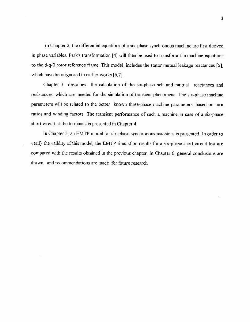
In this chapter, the differential equations for a six-phase synchronous machine and its

equivalent circuit model are derived. The synchronous machine is assumed to have six identical

windings in the stator, in which they are divided into two symmetrical three-phase sets, called a-b-

c and x-y-z. The three-phase system x-y-z is displaced with respect to the system a-b-c by 30°.

The three rotor windings are the field winding f, that produces flux in the direct axis, and two

equivalent damper windings D and Q in the d- and q-axes. These nine windings are magnetically

coupled, and the magnetic coupling between the windings is a function of the rotor position.

Figure 2.1 shows a cross section of the synchronous machine with its six stator and three rotor

windings.

# z-axis^rotor d-axis

Figure 2.1: Cross Section of Synchronous Machine4

5

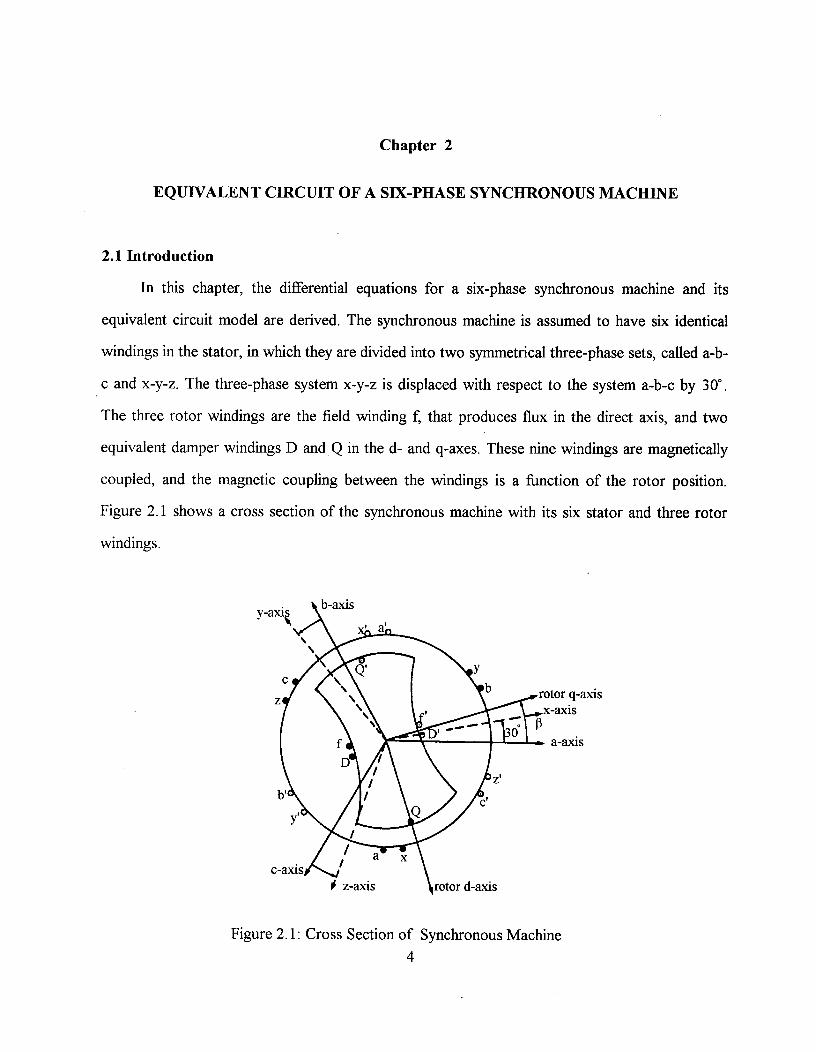
2.2 Differential Equations

The voltage-current-flux relationship of the 9-coil machine in Figure 2.1 is described by the

following equations:

[v] = [R][ddt [x];

[2] [L][d;

f ) ID ,

[v] = [va,vb,vc,vx,vy ,vz ,v f ,0,0 ;

[11]={2a52b)11c,i1x,2y3/1"z,2 f,2D,2Q]T ;and

[R] = diag[ra ,ra ,ra ,ra ,ra ,ra ,rf ,rD ,rQ ].

The elements of the matrix [L] describing the linkage between the fluxes [X] and the currents [i]

depend on the rotor position 13:

[L] = [Lu (0•^ (2.7)

With all the coils having the same number of turns, or with rotor quantities referred to the stator

side, the elements Lu of the matrix in equation 2.7 are given bellow [5] (the lower case "

represents the leakage inductances).

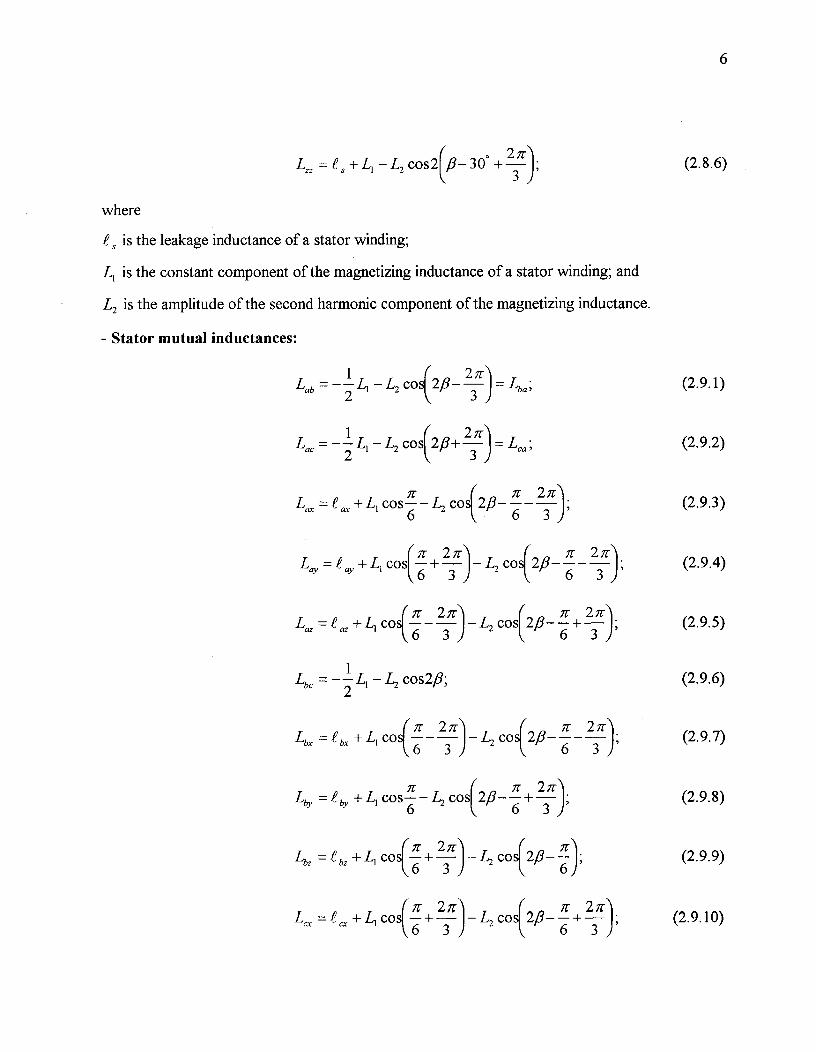
- Stator self inductances:

▪ +L1Laa = ^11 – 1,2 cos2,8;^ (2.8.1)

7"1"Lbb =^

2

•

L1 – L2 cos2(fi– —31;^ (2.8.2)

Lac = s + 11 -4 cos2(f3+ 1.2 );^ (2.8.3)3

L,, = e + L i – 1,2 cos2G6-- 301;^ (2.8.4)s

(2.1)

(2.2)

(2.3)

(2.4)

(2.5)

(2.6)

Lyy =L 5 +L1 –LZ cos2l/3-30 ° – 371;^(2.8.5)

6

Lzz = e + L, — L2 cos2(fi— 30 °

where

(2.8.6)+ —231;

.e s is the leakage inductance of a stator winding;

L, is the constant component of the magnetizing inductance of a stator winding; and

L2 is the amplitude of the second harmonic component of the magnetizing inductance.

- Stator mutual inductances:

1—^1 — L2Lab^—2.L2

Lba; (2.9.1)2flcos^—3

1Lac = — — Li — L22

L.; (2.9.2)71-)=COS(213 + —23

7rLax =^+L, cos—6

—^cos(^7r^2r

32,^—

6 — —); (2.9.3)

Lay = t ay + L,cos(Lr3 -1— L2 cos7r

2,3- 727r1 (2.9.4)— —3 ;

La, =^az + Li cos —

n- — —

2 7r^27r— L2 COS(2)6 — —+—);

6^3(2.9.5)7r)

6^3

1L

b'^—2

LI — 1,2 cos2fi; (2.9.6)

Lbx^bx^L, cos( 7r^27r — L COS 2flLr6

(2.9.7)—6^3

27r) •3

Lby = "e by +^f=cos^—^COS(2g— 671-

6(2.9.8)2

3 71)-± '

Lb:^bz + Li cos( 7I^2 71" — L2 cos 7"C2/3--6

; (2.9.9)6— + —

3

27rL, =^+ L,cos(-7C + —)— L2 cos 7C210— 2g (2.9.10)36^3 6

7

27z-Lc, = +^cos(— — — L2 cos 2)3-6); (2.9.11)6^3

L = +L, cos 1,27- (2.9.12)cos(2fl —^_ 2 31 ;

where

ax , f ay , f a, are the mutual leakage inductances between phase a and phases x, y and z;

bx , 'e by)"e bZ are the mutual leakage inductances between phase b and phases x, y and z; and

are the mutual leakage inductances between phase c and phases x, y and z.

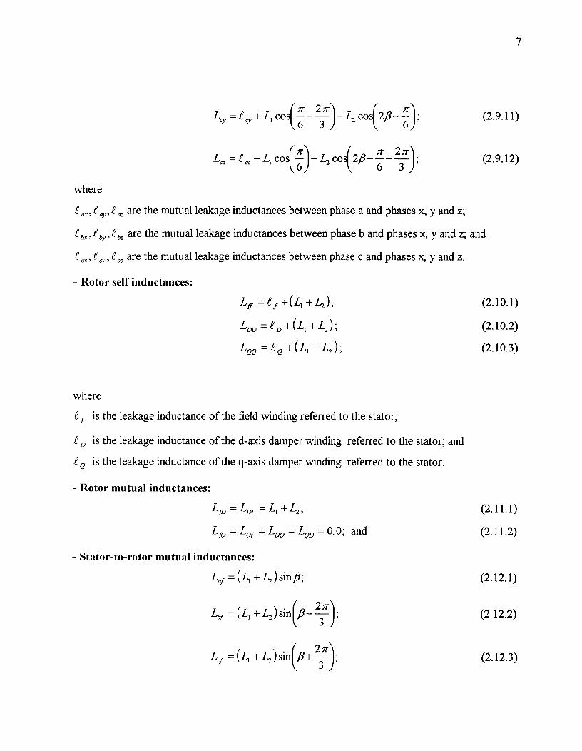
- Rotor self inductances:

Lff = t f + (Li + L2 ) ;^ (2.10.1)

LDD =^+(LI + L2 );^ (2.10.2)

L„ = t + (L 1 — L2 );^ (2.10.3)

where

f is the leakage inductance of the field winding referred to the stator;

.e r, is the leakage inductance of the d-axis damper winding referred to the stator; and

Q is the leakage inductance of the q-axis damper winding referred to the stator.

Rotor mutual inductances:

Ln, = Lpf -7, L, + L2 ;^ (2.11.1)

LiQ = LQt = LDQ = LQD = 0.0; and^ (2.11.2)

- Stator-to-rotor mutual inductances:

Laf = (L1 + L2 )sinf3;^ (2.12.1)

Lbf = (Li + L2 ) sin(fl— 31;^ (2.12.2)

Laf =( L, + L2 ) sin (fl+ —2371;^ (2.12.3)

Lxf = ( L1 + 4 ) sin (fi— , r);

Lyf (L, + L2 ) sin (fl— 2,3r — Y-);

=(L+ L2 )sin(fi—:- + 2-31;

Lap = ( L 1 + 4 )sin

LbD = ( L1 + 1,2) sin( —23

LCD = ( L, + L2 ) sin(fl+

LxD = (Li + L2 ) sin(13 r);

LyD (L1 + L2 ) sin(fl-

LZD = (Li + L2 ) sin (fi— 6+ y);LaQ = (Li — ) cos/3;

2 7rLbQ = (L1 — L2 ) co?— —3--);

LcQ^1=(L — 1,2 )cos(fi+ —237r);

L„Q, =(11 — 1,2 )cos^—6);

2 71"L yo = (L1 — L2 ) cos(/3 — ^—

3);

(2. 12.4)

(2.12.5)

(2.12.6)

(2.12.7)

(2.12.8)

(2.12.9)

(2.12.10)

(2.12.11)

(2.12.12)

(2.12.13)

(2.12.14)

(2.12.15)

(2.12.16)

(2.12.17)

9

7T 2 71"LZQ = (11 — ) COS^

613– — + — .

3(2.12.18)

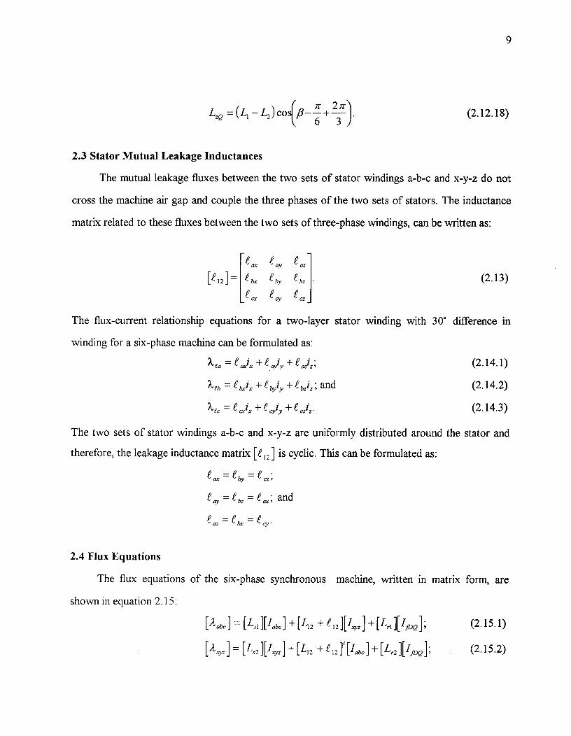
2.3 Stator Mutual Leakage Inductances

The mutual leakage fluxes between the two sets of stator windings a-b-c and x-y-z do not

cross the machine air gap and couple the three phases of the two sets of stators. The inductance

matrix related to these fluxes between the two sets of three-phase windings, can be written as:

t ax ,t ay f a,

e 12] – ebx f by f bz^ (2.13)

cy^cz

The flux-current relationship equations for a two-layer stator winding with 30° difference in

winding for a six-phase machine can be formulated as:

?t, ta = atfx^+ G aziz ;^

(2.14.1)

X = L bxlx + byi y + e bzi z; and^

(2.14.2)

sec – L cxix^cyiy + cziz^ (2.14.3)

The two sets of stator windings a-b-c and x-y-z are uniformly distributed around the stator and

therefore, the leakage inductance matrix rp 12] is cyclic. This can be formulated as:L -

= C by = cz;

f ay = f bz^a,; and

t az = fbx = cy

2.4 Flux Equations

The flux equations of the six-phase synchronous machine, written in matrix form, are

shown in equation 2.15:

[Aabc = [41 ][Iabc^[112 + £12^[Lri ][Ifiv ] ;^(2.15.1)

[2xyz = [Ls2^+[L, 2 +^[lab,]+ [1, ,][IIDQ];^

(2.15.2)

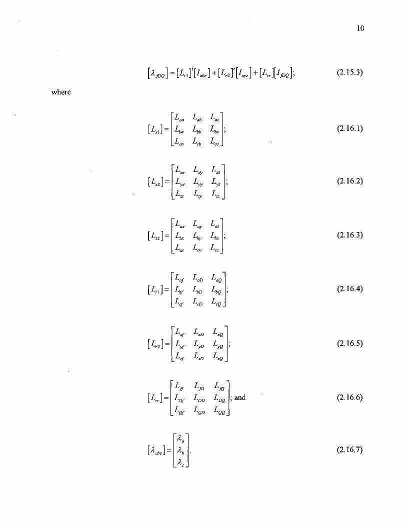
where

10

[2.1,Q]=[L,J[la,]+[L,,2]`[I,,z]+[L,][1],d; (2.15.3)

[Lsi ] =Lac,

Lba

Lab

Lbb

Lac

Lbc (2.16.1)_L„ Lth L„

[42]_

L.Lam.

L,„

Lam,

L,,L2,,

Lay

Lyz

L„

Laz

(2.16.2)

[ 1,12 ]= Lbx Lby Lbz (2.16.3)L,

LLaf

Lay

L

L„

L aQ[4 1 ] = Lbf LbD LbQ (2.16.4)

L LCD LcQ

L L LxQ

[42 ] , L yf

L zf

LyD

L zD

L yQ

LzQ

; (2.16.5)

Li . L JD Liu

[1,„ ]= L Df LDD LDQ ; and (2.16.6)L Qf LQD LQQ

(2.16.7)

[ T] =^[T,^ 0^0

^0^[T ]]

^0 ^0^x„

(2.17)

with

11

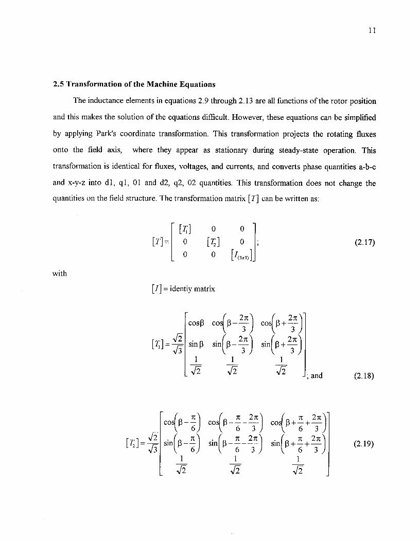
2.5 Transformation of the Machine Equations

The inductance elements in equations 2.9 through 2.13 are all functions of the rotor position

and this makes the solution of the equations difficult. However, these equations can be simplified

by applying Park's coordinate transformation. This transformation projects the rotating fluxes

onto the field axis, where they appear as stationary during steady-state operation. This

transformation is identical for fluxes, voltages, and currents, and converts phase quantities a-b-c

and x-y-z into dl, ql, 01 and d2, q2, 02 quantities. This transformation does not change the

quantities on the field structure. The transformation matrix [T] can be written as:

[I] = identiy matrix

cosI3 cos p - —1■4„ 2

^

3 ^cost/(3

233

sing sin(13 - 2-2 c ) sin(f3+ Lc )3

1^1 3^1

; and^(2.18)

cos` —1 cos 13- —7c — —27c) COS 13 ± —71 + —27c )6^6 3^6 3

sin(13- a6 ) sin(13 -6 — —27c) sin(I3 + 1-c +3^6 3

1^1^1

(2.19)

12

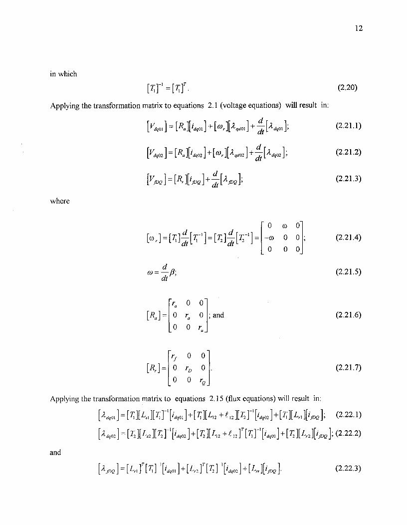
in which

[T]1 = [T]r^ (2.20)

Applying the transformation matrix to equations 2.1 (voltage equations) will result in:

[Vdoi] = lidgod [cor]{2ood+ ydt [2401];^(2.21.1)

[V dqO2] [Ra][' dg02] -1- [ a r][2 qd02] + —dd^dq02 ;^(2.21.2)

[17iD2 ] , [Rr ][iiD2 + Tit [2.11V ];^

(2.21.3)

where

0 o) 0[co r [Ti]ddt [T]ddt [ 7,2- 1

–0) 0 0 ;0 0 0

(2.21.4)

co = —d fi;^ (2.21.5)dt

[Ra ] =ra

00r a

0 -0 ; and

0 0 ra

rf 0 0

[Rd = 0 rD 0

0 0 Q

(2.21.6)

(2.21.7)

Applying the transformation matrix to equations 2.15 (flux equations) will result in:

[2 dqOI] – [ 71 Lsl][T] 1 [i dq01] [ TI][ L12^121-172] 1 [I iq02] + [1il

1][ Lrl][i !EV ];^(2.22.1)

[2 clq02] = [ T2][Ln][T2] -1 [i cio2]±[T2][ 112 e 12 f [ nidq01] + [ T2 ][42 ][iim2 ]; (2.22.2)

and

[2„2 ] = [Lri ]T [T1 ] -1 [idol ]+ [L, ]T [7;][idg02 ] + [Lrr ][ipd.^(2.22.3)

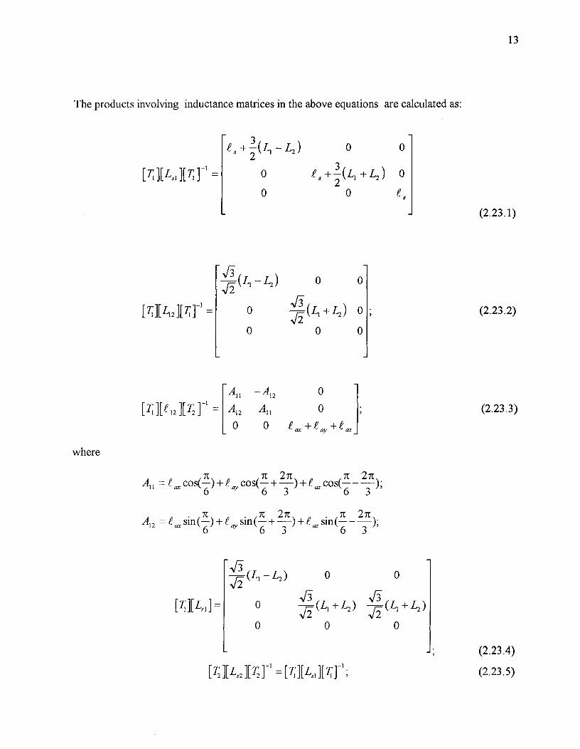
The products involving inductance matrices in the above equations are calculated as:

13

[TaLsa ] =

+ -23 (L I - L2 )^0^0

0^ts+2(LI -1-L2 ) 0

0^0^S

(2.23.1)

(L — L2)^0^0

[ 7142 I T1 = (2.23.2)-Nh+ 1,2) 0

o^o

][ T2 ] 1 = (2.23.3)

where

Ail = ar cos(16-1 )-F ay cos(: + 37---t )+ t cos( 2 ;A:^315

Al2 =t ax sin(:) +f ay sin( +^-1e az sin( 716 ^)

(Li — L2 )^0^

0

o^+ 1.2) 13-

(LI ± )

0^0^0[Ti][Lri =

(2.23.4)

(2.23.5)[12 ][i-s2^r = [TILATI ;

14

[T2][LI2f[Ti] 1 = [ 711,121 7'2r ;

Elatun Td -1 ={[TileidT2Y[}T;

[la42]=[1141];

[L,]T [Ti ]-1 .{[Td[4jy;and

[42]T[T2r ={[T2][42] } T

(2.23.6)

(2.23.7)

(2.23.8)

(2.23.9)

(2.23.10)

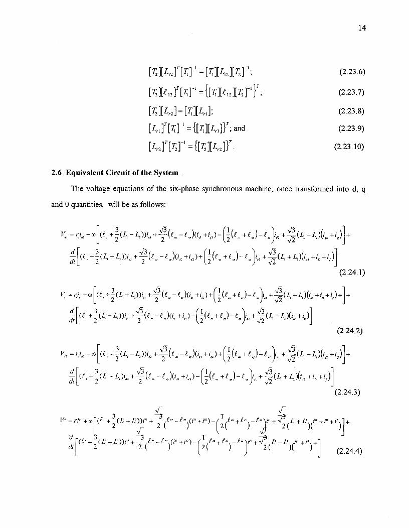
2.6 Equivalent Circuit of the System

The voltage equations of the six-phase synchronous machine, once transformed into d, q

and 0 quantities, will be as follows:

+3

(L, -^ - t „,)(io +io )-(-kt + t )-t i„+ ,̂

•

(L, Lz )(ig +i)]+2^2 -^2 '

dt^

-V2^2

ArJ,^1,

2^-^2 "^"d[ (^-3 (Li + L2))ia,+—

2 kt - t ,)(ia,+id2 )+(kt + t^t^+ L2 )(„+i,,+if )]I

(2.24.1)

V =ri +o)[(t,+-3 (L+L,))id,+ —

2 kt

dt^2^Lmi,,+2(t..—e,)(i,, • )^+^-^+0]

(2.24.2)

(t ,+-(Li - L2 ))i,2 +—

2 kt^t

"

)(i +i,2)+(-kt + t )-^+

Aff

•

(L, L2 )(ig2

+i2 )11-

2 "/

^(t ,+-23 (L,+ L2)id2+

2 V

-

- t i(ia,+04-kt erc

\

•+1 )- t^,+^ (LI +1,2 )(id2 +iD +if )]2^q

^Vj^1 I

(2.24.3)

-,1—^-.I—3P=ri"+6..)(t +

3 (L + D))ia2 +^(^21- --1°, \

)(id' +id2)-(1-

( 1" +1-

) --t-V°' + V3

( L' +1,1

)( id' +i° +if +

2^2 ^2^)-,1— --da^-3dt (e' +

s (L - L))i" +^(^2t" ---e-

),(P' + l' 1 ) - (1-

(^2t" -ft'

)\ --t - \e+V3

( L' - L2

)( io + P

) +[^2^2^1 ^ (2.24.4)

vdl = ria, — [(

Vd2^raid2

dt

15

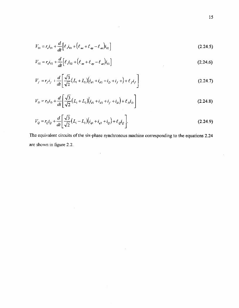
V0 , , ra i01 +dt

[. sio,+(t^t ay – t Jicei

V02 = rai02 +dt

[t 102 +(t ax + t ay – t

Vf =r

f i +—d [—(L +1.2)(idif dt

d [ NdVD ="

+ L2 )(id ,dt 1/2

d [VQ

=rQ iQ

+—dt 15

^–L2 )(iql +ig2 ±/Q )+e Q/Q

(2.24.5)

(2.24.6)

(2.24.7)

(2.24.8)

(2.24.9)

1+id2 -ElD +1f -0 - F .e fif

1-Fid2 -Fif -FiDke DiD

The equivalent circuits of the six-phase synchronous machine corresponding to the equations 2.24

are shown in figure 2.2.

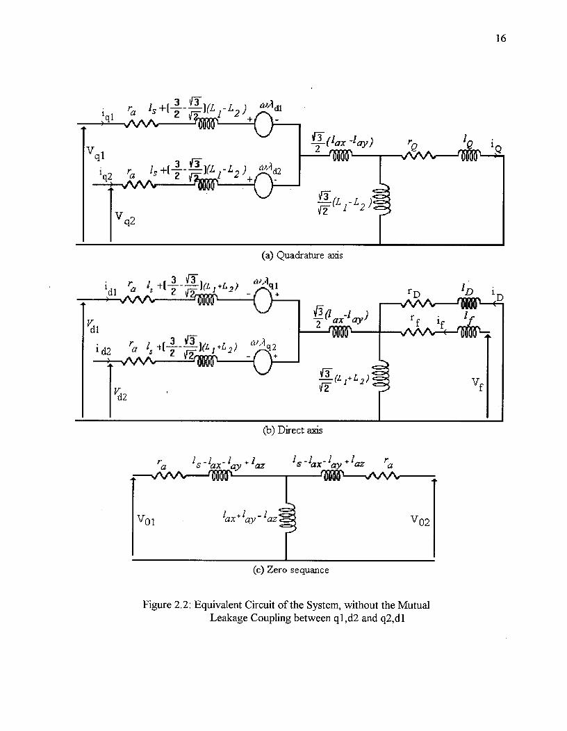
16

Figure 2.2: Equivalent Circuit of the System, without the MutualLeakage Coupling between ql,d2 and q2,d1

Chapter 3

SIX-PHASE MACHINE PARAMETERS

3.1 Introduction

In this chapter, the six-phase synchronous machine reactances and resistances will be

derived, assuming that the machine is constructed by splitting each 60° phase belt of a three-

phase machine into two equal 30° phase belts, one for each three-phase winding set [8]. The six-

phase machine parameters will be related to those of the three-phase machine, based on the turns

ratios and winding factors.

3.2 Synchronous Self-Reactances of a Three-Phase Machine

For a three-phase salient pole synchronous machine with N3 equivalent stator turns per

phase, the reactances in the rotor reference frame can be written as [9]:

Xd 3 = co-3 N 2P : and3 ^3 d

Xq3 = w NP •2 3 q5

wherePd is the d-axis equivalent permeance dependent on machine dimensions;

P is the q-axis equivalent permeance dependent on machine dimensions;

co is the base frequency; andN3 is the turns per coil of a three-phase machine.The subscript 3 is used to denote three-phase machine values.

(3.1.1)

(3.1.2)

3.3 Stator Leakage Reactances of a Three-Phase Machine

The stator leakage reactances will be derived assuming that the stator winding has two

layers with sixty degree phase belts, and that the winding phase belt has either unity or 5/6 pitch.

In both cases, the leakage reactances can be divided into two distinct components:17

18

(a) slot dependent leakage reactance;

(b) all non-slot related leakage reactance including zigzag-leakage reactance, the belt-

leakage reactance, and the coil end leakage reactance.

From the above definitions, the leakage reactances of a three-phase machine can be written as:

Xes. = Xe + XPsiot^ (3.2)

where

Xeslot is the slot dependent leakage reactance; and

Xe is the sum of all non-slot related leakage reactances.

- Slot leakage reactances

The slot leakage reactances are made up of three parts: the self reactance of the coil sides in the

top; the mutual reactances between top and bottom layer coil sides in the stator slots and the self-

reactances of the coil sides in the bottom.

X toot = Xer ± KS XeTB + X eB^ (3.3)

where

X iT is the slot leakage reactance due to coil sides in the top;

Xe.„ is the slot leakage reactance due to coil sides in the bottom;

XeTB is the slot leakage reactance between top and bottom layer coil; and

K is the coupling factor that is dependent on the winding pitch.

The slot leakage reactance components in equation 3.3 are each defined as:

A T 2 T PTX a = COIY 3 L.

" 3

XpB CON3 2 LS3

XtTB cDN32 L TB

3

(3.4.1)

(3.4.2)

(3.4.3)

where

19

PT ,P, are the permeances in top half and bottom half of the slot;

Pm is the permeance of mutual coupling between coils in the top and bottom half,

L is the slot length;

N3 is the turns per coil of a three-phase machine; and

S3 is the number of stator slots per phase of the three-phase machine.

For a three-phase winding, the effective value of the coupling factor Ks will vary linearly with

pitch, so that for pitch values p between 2/3 and 1 [9]

Ks =3p —1.^ (3.5)

Substituting equation 3.5 into 3.3 results in the following slot leakage reactances:

for a unity pitch^ Xeslot = X€7, + 2 X trB ± X tB ; and^ (3.6.1)

for a 5/6 pitch ^Xesiot = XP7' +1 ' 5X/TB + X .^ (3.6.2)

- Non-slot leakage reactances

The non-slot leakage reactances are approximately proportional to the square of the equivalent

stator turns and base frequency,

XP = coKiN3 2 ,^ (3.7)

where

Ke is the proportionality factor dependent upon the end winding and slot dimensions and the

number of turns per pole.

3.4 Relating Six-Phase Machine Parameters to a Three-Phase Machine

A six-phase machine can be constructed by splitting the 60 degrees phase belt of a three-

phase machine into two equal portions each spanning 30 degrees. This technique is illustrated in

figure 3.1 for a machine having six slots per pole.

(3.8.1)

(3.8.2)

(3.8.3)

N =6^2 K pd,

K _ Kp6Kd6

pd Kp3Kd3

S6S3

2

20

a-c

-c-c

-cb

b

-a-a-a

-a -b-b

-b

(a)

a

x

-c-c-z

-zb

b

-a

(b)

6 -b

Mc turns

0 -b

tic turns

aa

b

b

ax

-b^-Y-v

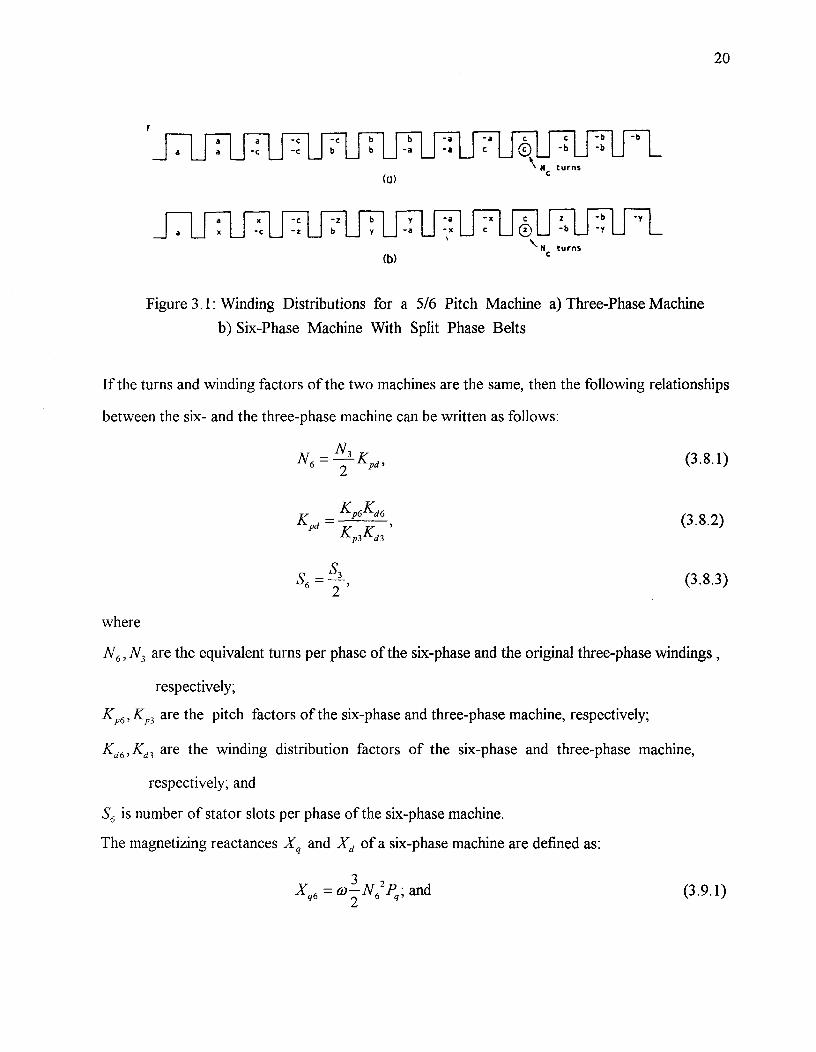
Figure 3.1: Winding Distributions for a 5/6 Pitch Machine a) Three-Phase Machineb) Six-Phase Machine With Split Phase Belts

If the turns and winding factors of the two machines are the same, then the following relationships

between the six- and the three-phase machine can be written as follows:

where

N6 , N3 are the equivalent turns per phase of the six-phase and the original three-phase windings ,

respectively;

Kp6 ,Kp3 are the pitch factors of the six-phase and three-phase machine, respectively;

Kd6 , Kd3 are the winding distribution factors of the six-phase and three-phase machine,

respectively; and

S6 is number of stator slots per phase of the six-phase machine.

The magnetizing reactances Xq and Xd of a six-phase machine are defined as:

X = co-3 N 2P andq6 2 6 ql (3.9.1)

21

2 Pw— N6 2^6 d • (3.9.2)

From equations 3.8 and the impedance relationships of equations 3.1 and 3.9 , the following

equations relating six-phase parameters to their three-phase counterparts can be derived:

Xq6 = X0-14 (Kpd ) 2 ;

X d6 = Xd3 741 (Kpd ) 2 ;

(3.10.1)

(3.10.2)

X tQ6 = X to 4-1- (K pd ) 2 ; (3.10.3)

/^2XiD6 = XiD

3 4 VC d—

1^)

P•• (3.10.4)

X if 6 = X tf 3 —14 (Kpd )2 ; (3.10.5)

1^N2r^=r^ 1CpdQ6^Q3 4 ( (3.10.6)

1^\ 2rD6 = rD3^

Pd) • and (3.10.7)

r^=r^-1-(K^) 2f 6^f 3 4^pd^' (3.10.8)

The stator resistances of a six-phase machine are directly proportional to the number of stator

turns, as in the case of a three-phase machine. Therefore, for an even stator split, the stator

resistance will be

1ra6

2r a3 • (3.11)

3.5 Stator Leakage Reactance of a Six-Phase Machine

As in the case of a three-phase machine the stator leakage reactances of a six-phase machine

can be broken into two parts:

22

Xis = Xt6 + X •

where

Xtriot 6 is the slot dependent leakage reactance of a six-phase machine; and

X16 is the sum of all non-slot related leakage reactances of a six-phase machine.

The slot leakage reactance can be broken into three components so that

Xts1ot6 = XiT6 Ks6X17736 + X06'

(3.12)

(3.13)

For the same number of turns per pole of the three-phase machine, each component of equation

3.13 can be defined as:

XiT6 = ON 2 /,6 s6

PXt B 6 = CON62 s6

2 ^X ^coN L TB€TB 6 —^6^ckl 6

(3.14.1)

(3.14.2)

(3.14.3)

where

Ks6 is the coupling factor that is dependent on the winding pitch.

As with the three-phase case, the coupling factors Ks6 vary linearly with the pitch factor p

Ks6 12p-10 for 5 5p<_ 1.6

(3.15)

From equations 3.13 and 3.15, the slot leakage reactance for a unity pitch can be written as:

X tslot6 XIT6 +2 XCTB6 + X CB6^ (3.16)

and for a 5/6 pitch factor

Xtslot 6 X176 + XCB6'^ (3.17)

The mutual leakage coupling between the two sets of windings is only caused by stator

winding from each three phase set occupying the same stator slot. Therefore, all mutual leakage

reactances can be related to XiTB6 by coupling factors:

23

X Pax KxXPTB6;^ (3.18.1)

Xtay KyX€TB6; and^

(3.18.2)

X taz = KzXtni. 6 .^ (3.18.3)

For a 5/6 pitch winding, the coupling factors can be determined by inspection of figure 3.1 as

follows:

Kx =1;^KY = —1; and Kz = 0,^for 5P =

6(3.19)

From equations 3.4 , 3.7 , 3.8 and 3.14 , the following relationships between the six-phase and

three-phase leakage reactances can be derived:

xt 6 = 3 Kpd ;1(^)2

X PT6 + Xle136 = 2(Xtr3 + XtB3 ); and

XiTB 6 = 12

A 1TB 3 •

(3.20.1)

(3.20.2)

(3.20.3)

3.6 Machine Parameters

The six-phase synchronous machine parameters will be derived from a three-phase, four pole,

salient pole, 125 kVA, 480 V synchronous machine whose parameters are given in table 3.1. For

a machine of this type, the slot component of the leakage reactance is 35% of the total leakage

reactance [9] and therefore

Xisolt 3

35= 0̂0 0.147) = 0.05145 f2 and1

(3.22.1)

65^\X€3 = 00 0.147) = 0.0956 a1

(3.22.2)

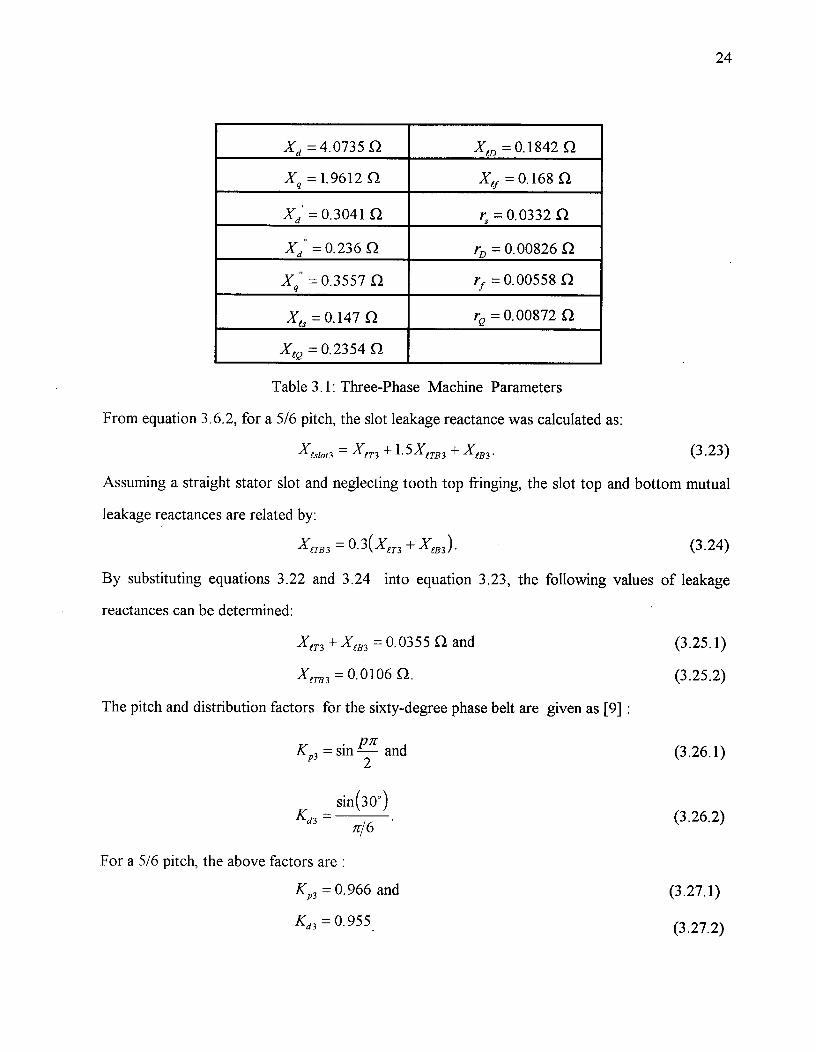
Xd = 4.0735 Q X ii3 = 0.1842 C2

Xq =1.9612 Q Xt./. = 0.168 nXd

' = 0.3041 52 rs= 0.0332 nx; = 0.236 Q rD = 0 ' 00826 Q

Xq = 0.3557 fl rf = 0.00558 fl

Xis = 0.147 fl rQ = 0 . 00872 nX€Q, = 0.2354 f2

Table 3.1: Three-Phase Machine Parameters

From equation 3.6.2, for a 5/6 pitch, the slot leakage reactance was calculated as:

Xis/0f 3 = Xin + 1.5 XiTB 3 + X a33 .

24

(3.23)

Assuming a straight stator slot and neglecting tooth top fringing, the slot top and bottom mutual

leakage reactances are related by:

X €TB 3 = 0.3(X€T3 + X 03 ) .^ (3.24)

By substituting equations 3.22 and 3.24 into equation 3.23, the following values of leakage

reactances can be determined:

X in + X tin -= 0.0355 f2 and

X erB 3 = 0.0106 Q.

The pitch and distribution factors for the sixty-degree phase belt are given as [9] :

Kp3 = sin —PIT and2

sin(30°)Kd =^

3^TC/6

(3.25.1)

(3.25.2)

(3.26.1)

(3.26.2)

For a 5/6 pitch, the above factors are :

Kp3 = 0.966 and^

(3.27.1)

K d3 = 0.955 .^(3.27.2)

25

From all the above parameters for a three-phase machine, their six-phase counterparts can now

be calculated.

- Six-phase synchronous machine parameters

The value of the pitch factor Kp is the same as in the case of a three-phase machine. However, the

value of the distribution factor will depend on the number of phase belts per pole and the number

of slots per phase belt:

Kd6

sin( 2q2q

n sin( n"2nqj

(3.28)

where

q is the number of phase belts per pole; and

n is the number of slots per phase belt.

For a 5/6 pitch the distribution factor is:

Kd6 = 0 . 989 .^ (3.29)

Substituting the values of Kp3 ,Kd3 ,Kp6 and Kd6 into equation 3.8.2 will result in

Kpd = 1.0356.^ (3.30)

Substituting the three-phase impedance values along with equation 3.30 into equation 3.10 will

result in the six-phase machine parameters that are shown in table 3.2. From equations 3.18, 3.19

and 3.20, the leakage reactances and the mutual leakage coupling are calculated and their values

are shown in table 3.3.

X d6 = 1.0921 f2 X iD6 = 0.0493 fl

X q6 = 0.5258 f2 X4/6 = 0.0437 f2

X d6 . = 0.0815 f2 rs6^.= 0 0166 Q

X d6 = 0.0633 f2 rf6 = 0 . 00149 Q

= 0.0953 0 rD = 0 . 0022 nXtQ6 = 0.0631 Q r

Q^'= 0 0023 0

Table 3.2: Six-Phase Machine Parameters

Xt6 = 0.0256 f2 Xta, = 0.0 f2

X €TB 6^0.0053 f2 Xtskt6 = 0.01775 f2

X tay = —0.0053 fl Xts6 = 0.0433 Q

Xtax = 0.0053 f2 X€7. 6 ± X tB6 = 0.01775 Q

Table 3.3: Leakage Reactances of the Six-Phase Machine

26

Chapter 4

TRANSIENT ANALYSIS

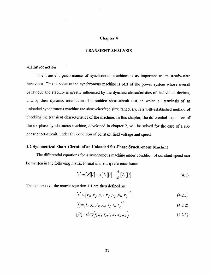
4.1 Introduction

The transient performance of synchronous machines is as important as its steady-state

behaviour. This is because the synchronous machine is part of the power system whose overall

behaviour and stability is greatly influenced by the dynamic characteristics of individual devices,

and by their dynamic interaction. The sudden short-circuit test, in which all terminals of an

unloaded synchronous machine are short-circuited simultaneously, is a well-established method of

checking the transient characteristics of the machine. In this chapter, the differential equations of

the six-phase synchronous machine, developed in chapter 2, will be solved for the case of a six-

phase short-circuit, under the condition of constant field voltage and speed.

4.2 Symmetrical Short -Circuit of an Unloaded Six-Phase Synchronous Machine

The differential equations for a synchronous machine under condition of constant speed can

be written in the following matrix format in the d-q reference frame:

[v] = [R ]p]^[ -Lid^[L2 ] [i ] •

^ (4.1)

The elements of the matrix equation 4.1 are then defined as:

[11]=[Vai ,Vgi ,Vd2 ,Vq2 ,V f ,VD ,Vd ;^ (4.2.1)

[i] [idl iql id2 ,iq2 if iD 3 1dr .3^ (4.2.2)

[R] = diag[r,„ra ,r„,r,„rf ,rp ,re ];^ (4.2.3)

27

0

28

0^IJI (t..-ti+(L, -4)^

0^L1-L,€.+;(4 -L2)^

0

2^2

-t,+2(L,+/.2)^0+1,2)^

-L -L,-4-L,^0

(1° ,+1,,,,)-1,,

2

--‘5 (e -C )- 2(L +L )2^°,^'^2 '^2

000

0 0 01(1.,,-1,,,,)+;(4- L2 ) 1, + ;(1., -4)

4/^+L^).-/2^"^'^"

-1,-1(4 +4)0 -L -1,.., -L,-L,

0 0 0 0 00 0 0 0 0

0 0 0 0 0

and

[4] =L,-L,

0

000_

(4.3)

^1, +(L, +4)^0

0^L,^-L,)

-/ )+ 2 (L, +L,)^2 " " 2 '^2

0

0

0

;(4-4)

)+(L +L2 " " 2^

)^2

4 (t,,,-t,,,,)+ 2 (L, -4)

,e,+2(L+1,2 )^0

t, +(L,-L2 )

0

0

-2-(4 -4)

L,+L2^L,+L,^0

0^ - L,

4+1.2^L,+L,^0

0^0^4-4

1,,+(L+L 2 )^L,+L,^0

L,+L,^1,,+(L+L,)^0

o^0^to+(L-L,)

[L, ]=

(4.4)

The elements of the inductance matrices [L 1 ] and [L2 ] with constant coefficients have already

been defined in chapter 2. However, for each three-phase set, the addition of currents in all three

phases will equal to zero. Therefore by knowing that i„ +iy +i2 = 0 or zZ = —(ix +iy ), the stator

mutual leakage inductances matrix of equation 2.13 can be simplified as :

P12 ] =

ay — C0 —e az

t ay —t az^0

0

ay^az

e^'e az

To solve equation 2.1 for the currents it must be rearranged as follow:

[L2 at [i ] = -[R][i] +0 [L. ][i]± [v],^ (4.5)

=^[R][d ± CD [L2^+ [1'2 ] I M'^(4.6)

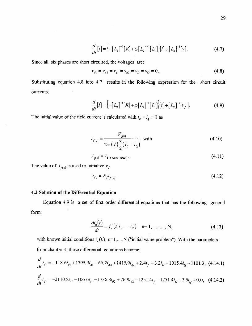
29

c",[i]= {—[4]-I[R]+co[4]1[L1]l[i]+[1,2]-1[v].^(4.7)

Since all six phases are short circuited, the voltages are:

Vdl — Vd2 — Vql — Vq2 — VD — VQ — 0 '^ (4.8)

Substituting equation 4.8 into 4.7 results in the following expression for the short circuit

currents:

',[i],{-[1,2 ]-1[R]+.[Li] 1[L1 ]}[i]+ [4]1[vi ].^(4.9)

The initial value of the field current is calculated with id iq = 0 as

Vq(0) N^ withf^\ 32m (f) (Li + L2 )

Vq(0) — Vt' —P rated (RMS) •

The value of if (0) is used to initialize vf ,

Vf 0 = Rfif (0) •

4.3 Solution of the Differential Equation

Equation 4.9 is a set of first order differential equations that has the following general

form:

di (t)n =f Vidt^n

^iN) n= 1,^ N,^(4.13)

with known initial conditions i,,(0), n=1, ^N ("initial value problem"). With the parameters

from chapter 3, these differential equations become:

—d

idi

= —118.6id,+1795.910 +66.21d2 +1415.91q2 +2.4if +3.2iD +1015.4/2 —1101.3, (4.14.1)dt

—dt

iql

= —2110.81d , — 106.610 —1736.8/d2 +76.9iq2 —1251.4if —1251.4/D +3.5/2 + 0.0, (4.14.2)

30

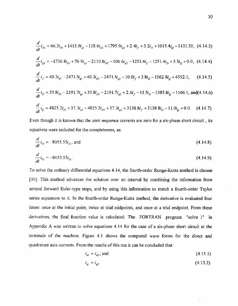
dt

-

id2

= 66.2id, +1415.9i0 –118.6id2 +1795.9iq2 +2.41f +3.2iD +1015.4iQ –1101.30, (4.14.3)

—d

iq2

= –1736.81d , +76.9ig , –2110.81d2 –106.61q2 -1251.41f –1251.4iD +3.5iQ +0.0, (4.14.4)dt

d

-

if = 40. 3id, – 2471.510 + 40.31d2 – 2471.51g2 – 10. Oif + 3. 8iD – 1562. 8iQ + 4552.1,^(4.14.5)

dt

—d in = 35.81d , –2191.7i0 +35.8id2 –2191.71q2 +2.6if –13.5iD –1385.8iQ –1166.1, and(4.14.6)dt

dt -

-

= 4825.2id , +37.3ig , +4825.2id2 +37.3/q2 +3138.8if +3138.8iD –11.0ig, +0.0^(4.14.7)

Even though it is known that the zero sequence currents are zero for a six-phase short circuit , its

equations were included for the completeness, as:

—d i

•

°1 = –8055.55i01 , and^

(4.14.8)

dt—d

in, = –8055.55102 .^ (4.14.9)

To solve the ordinary differential equations 4.14, the fourth-order Runge-Kutta method is chosen

[10]. This method advances the solution over an interval by combining the information from

several forward Euler-type steps, and by using this information to match a fourth-order Taylor

series expansion to it. In the fourth-order Runge-Kutta method, the derivative is evaluated four

times: once at the initial point, twice at trial midpoints, and once at a trial endpoint. From these

derivatives, the final function value is calculated. The FORTRAN program "solve 1" in

Appendix A was written to solve equations 4.14 for the case of a six-phase short circuit at the

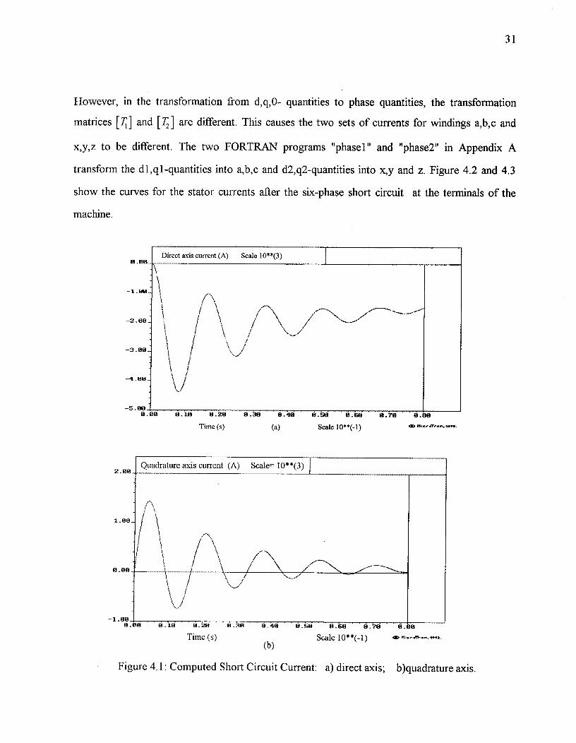
terminals of the machine. Figure 4.1 shows the computed wave forms for the direct and

quadrature axis currents. From the results of this run it can be concluded that:

id1 = id2 ; and^ (4.15.1)

1ql = q2 •^ (4.15.2)

uadrature axis current (A) Scale= 10**(3)

1.00_

00

—1 BB^8.08^8.18^8.13^. 6.13^8.48^0. 58^0. 68^0.78^0.88

Time (s)^ Scale 10**(-1)^CD Mic•-$11-...,:ssz.

(b)

2.00

31

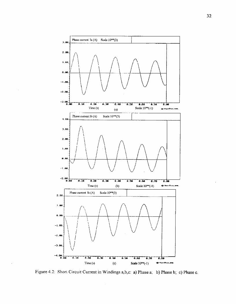
However, in the transformation from d,q,0- quantities to phase quantities, the transformation

matrices [Ti ] and [7'2 ] are different. This causes the two sets of currents for windings a,b,c and

x,y,z to be different. The two FORTRAN programs "phasel" and "phase2" in Appendix A

transform the dl,q1-quantities into a,b,c and d2,q2-quantities into x,y and z. Figure 4.2 and 4.3

show the curves for the stator currents after the six-phase short circuit at the terminals of the

machine.

0 BB

Direct axis current (A)^Scale 10**(3)

- .813

—2.00

—3.00

—4.88

—5 00

0.00^

8.18^8.20^

0.38^8.48^

8.50^8.60^

8.70^

8.88

^Time (s)^(a)^

Scale 10**(-1)

Figure 4.1: Computed Short Circuit Current: a) direct axis; b)quadrature axis.

32

Figure 4.2: Short Circuit Current in Windings a,b,c: a) Phase a; b) Phase b; c) Phase c.

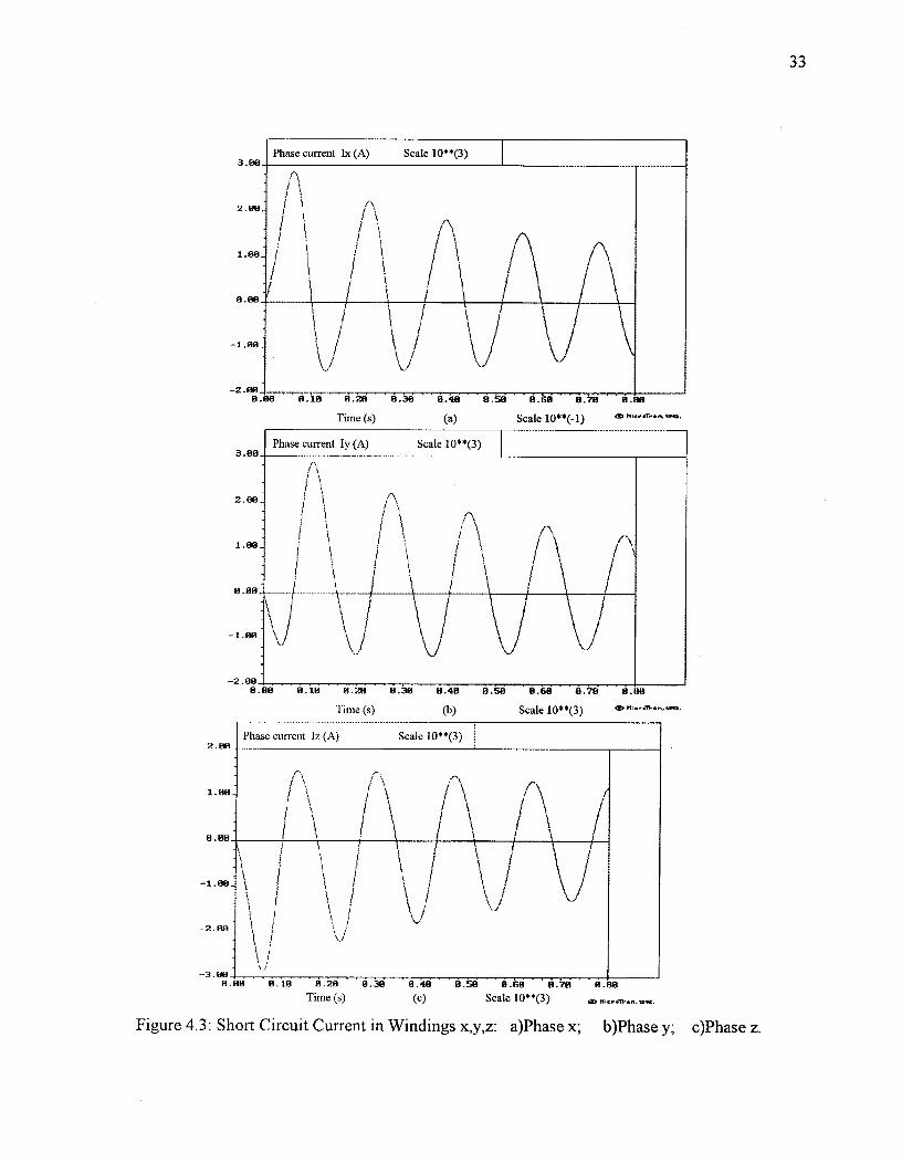
Figure 4.3: Short Circuit Current in Windings x,y,z: a)Phase x; b)Phase y; c)Phase z.

0.08 0.48^8.50^8.60^0.70^0.800.18^8.28^8.38

Time (s) (a) Scale 10**(-1) (4 111 e elre An. nfa.

Time (s) (b) Scale 10**(3) Mi•rell.•■•■.1sva.

0.58^0.68 ^82e0^8.66

Scale 10**(3)8.00 8.18^8.20

Time (s)0.30 8.48

(c) ED Mit D. 71-an. tflGt.

Phase current Ix (A) Scale 10**(3)

.

ii Y \I

f I ‘I i Ii 1 f■i

1 1I

I\ 1. 1/

\\ !

\

i

I^\^(,\

\ I^\

\i' \\i,/^\ \\

-2 080.80^8.10^8.20^8.30^0.48^0.58^0.68

Phase current Iz (A) Scale 10**(3)

._

r/, \ .,•.,\i e/) \

it I^\'''\

7 \\ I^\ \ I

\'I

11 1

‘ /I t t \ / t.

\ /t

f\ t \ /

.1

1I„..

\^1V

33

2 HO

1.80

08

- 1.08

-2.00

-3 00

3.08

2.08

1.08

8 88

-2.08

Field current If (A)^Scale 10**(3)8 00

7.00

6.00

5.08

4.88

3.00

2.00

1.08

8.18^8.28^8.38Time (s)

8.58^8.68^0.78Scale 10**(- 1 )

0 088.80 8.48 0.88

it Micr■Than. "Ma.

34

The short-circuit armature currents in figures 4.2 and 4.3 consist of a exponentially decaying

unidirectional current and a superimposed sinusoidal current with decaying amplitude. The dc

components of the armature currents all decrease to zero exponentially with the same time

constant T. The initial values of these components depend upon the point in the cycle at which the

short-circuit occurs. The ac component can be separated into, steady, transient, and subtransient

components. The transient component with a long time constant 7'; and the subtransient

component with a very short time constant Td".

Figure 4.4 shows the field current, which like the

armature current consists of dc and ac components. The dc component can be divided into

steady, transient, and subtransient components. The transient and subtransient dc components

decrease with the time constant Td ,

and Td . The ac component of field current decay with time

constant T, which is the same as the dc component of the armature currents.

Figure 4.4: Field Current After a Short-Circuit

Chapter 5

EMTP MODEL FOR THE SIX-PHASE SYNCHRONOUS MACHINE

5.1 Introduction

The Electromagnetic Transients Program is a general purpose computer program whose

principal application is the simulation of transient effects in electric power systems. It was

developed by H.W. Dommel in the late 1960's at the Bonneville Power Administration [11]. The

U.B.C. MicroTran version of EMTP has a model for a three-phase synchronous machine, in

which the electrical part of the machine is modelled as an equivalent two-pole machine with seven

windings [12]. These windings are: three armature windings; one field winding which produces

flux in the direct axis; one winding in the quadrature axis to represent fluxes produced by eddy

currents; one winding in the direct axis and one winding in the quadrature axis to represent

damper bar effects. In this chapter, an EMTP model for a six-phase, salient pole synchronous

machine, that includes the stator mutual leakage inductances, will be developed. This is achieved

by paralleling two identical three-phase synchronous machines in such a way that the magnetic

coupling between the two machines is included. The magnetic axes of the two three-phase sets are

displaced by an angle of 30° . The windings of each set are uniformly distributed and have axes

displaced 120° apart. In the first part of this chapter, the equations and the physical aspects of the

model will be discussed. In the second part, the EMTP model will be tested by simulating a six-

phase short circuit test at the terminals of the machine. The results of this simulation are then

compared against the results obtained from chapter 4.

5.2 Model of the Machine

The first proposal for including a multiple coil synchronous machine in the EMTP was

based on the fact that the magnetic coupling between the two three-phase sets can be

35

411

d2

q2

402

36

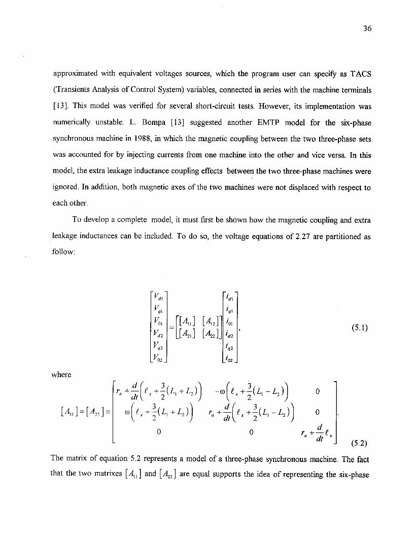
approximated with equivalent voltages sources, which the program user can specify as TACS

(Transients Analysis of Control System) variables, connected in series with the machine terminals

[13]. This model was verified for several short-circuit tests. However, its implementation was

numerically unstable. L. Bompa [13] suggested another EMTP model for the six-phase

synchronous machine in 1988, in which the magnetic coupling between the two three-phase sets

was accounted for by injecting currents from one machine into the other and vice versa. In this

model, the extra leakage inductance coupling effects between the two three-phase machines were

ignored. In addition, both magnetic axes of the two machines were not displaced with respect to

each other.

To develop a complete model, it must first be shown how the magnetic coupling and extra

leakage inductances can be included. To do so, the voltage equations of 2.27 are partitioned as

follow:

- Vd1

Vql

r [ Alli [Al2] -1L[A21] [A22]]

Vol

Vd2

Vq2

V

-

O2

^+—d^+ 1 ( i + L2 ))^dt^2

coLe s +-23 (L, +L2 ))-+ 3 /

,^-L2))^0

ra +-61 1.e s -E(L i -L2 ))^0dt

r +±-1 t0^ 0dt

where

] = [An ]

(5.1)

(5.2)

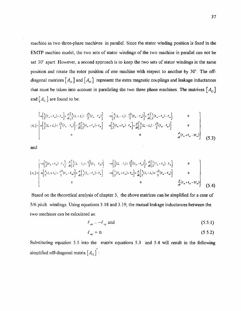
The matrix of equation 5.2 represents a model of a three-phase synchronous machine. The factthat the two matrixes [A„ ] and [A22 ] are equal supports the idea of representing the six-phase

37

machine as two three-phase machines in parallel. Since the stator winding position is fixed in the

EMTP machine model, the two sets of stator windings of the two machine in parallel can not be

set 30° apart. However, a second approach is to keep the two sets of stator windings in the same

position and rotate the rotor position of one machine with respect to another by 30°. The off-

diagonal matrices [Al2 ] and [4 1 ] represent the extra magnetic couplings and leakage inductances

that must be taken into account in paralleling the two three phase machines. The matrixes [A, 2 ]

and [4 1 ] are found to be:

oP (P„+/,)+t,P-P(4+/,,)+-1(t.—Pil2 dt 2 4)

+1(1. - €

.- )] + :7, [( t., + t w ) - ,-] 0

+ 4 )+ 1(c _^÷ i ,)+ t.]^

0

0^ 0^ d

(5.3)

and

2+e"

)—e^dt 2^2

—L )+—^-)^—4 3i (L,-4)+1(1.—i.)1+:71t [!(e.+e.)—e.]^0^-

[41= co[pL,+4)+ \fj.2 (e e,d+:7/ p2 „,+t,)_„]^_co[1(,„,+t,,)+,d,z(,_4)+1 (i.,_ed^

0

^0^ 0^1(t-+t.-2€.)^(5.4)

Based on the theoretical analysis of chapter 3, the above matrices can be simplified for a case of

5/6 pitch windings. Using equations 3.18 and 3.19, the mutual leakage inductances between the

two machines can be calculated as:

= --t ay and^ (5.5.1)

^az = 0.^ (5.5.2)

Substituting equation 5.5 into the matrix equations 5.3 and 5.4 will result in the following

simplified off-diagonal matrix [A, 2 ] :

d [(L +L)+ (t-cit 2^-^2^-

03[(L2, + L2 )±^

2 -

-4-3-(L1- +14-. (t _

d 3(L - L2 ) +^-e

38

01

0

0^ 0(5.6)

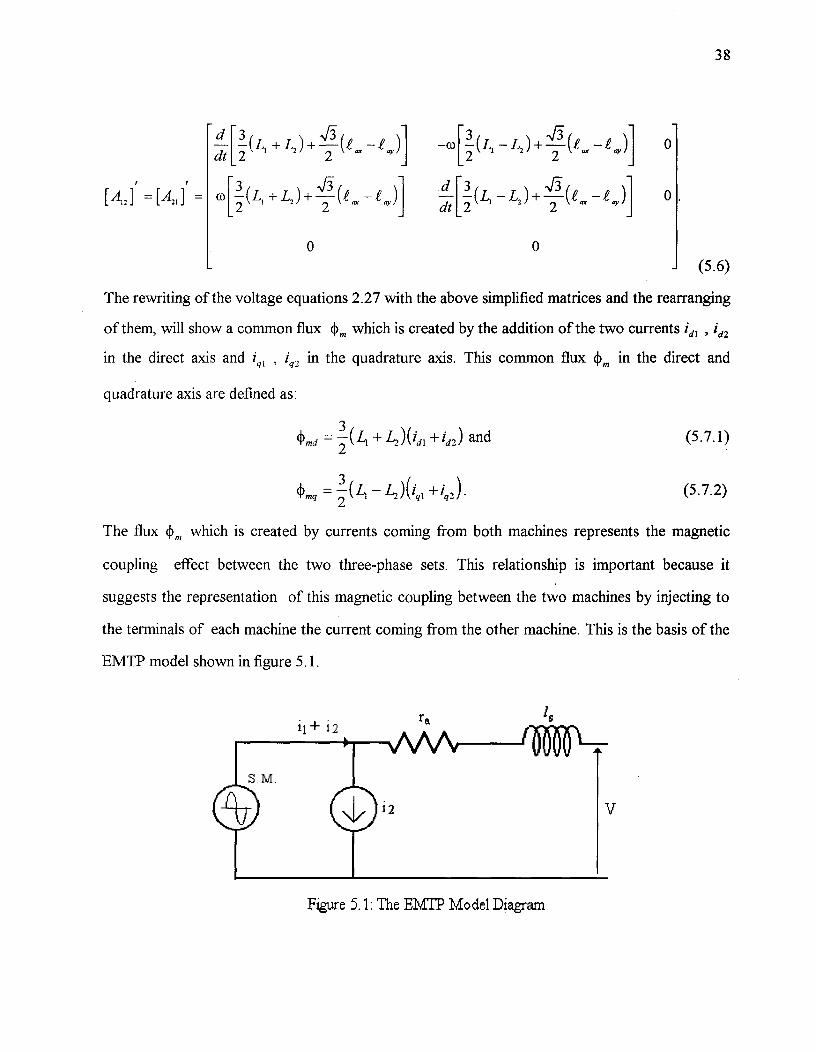
The rewriting of the voltage equations 2.27 with the above simplified matrices and the rearranging

of them, will show a common flux (I)„, which is created by the addition of the two currents id, d2

in the direct axis and igi , iq2 in the quadrature axis. This common flux 4m in the direct and

quadrature axis are defined as:

[ A,^= [A,,] =

,41) md

2^+ L2)( i dl^d2) and

11) =^L2)(mq^ iqlq2) •

(5.7.1)

(5.7.2)

The flux ,4),n which is created by currents coming from both machines represents the magnetic

coupling effect between the two three-phase sets. This relationship is important because it

suggests the representation of this magnetic coupling between the two machines by injecting to

the terminals of each machine the current coming from the other machine. This is the basis of the

EMTP model shown in figure 5.1.

Figure 5.1: The EMTP Model Diagram

39

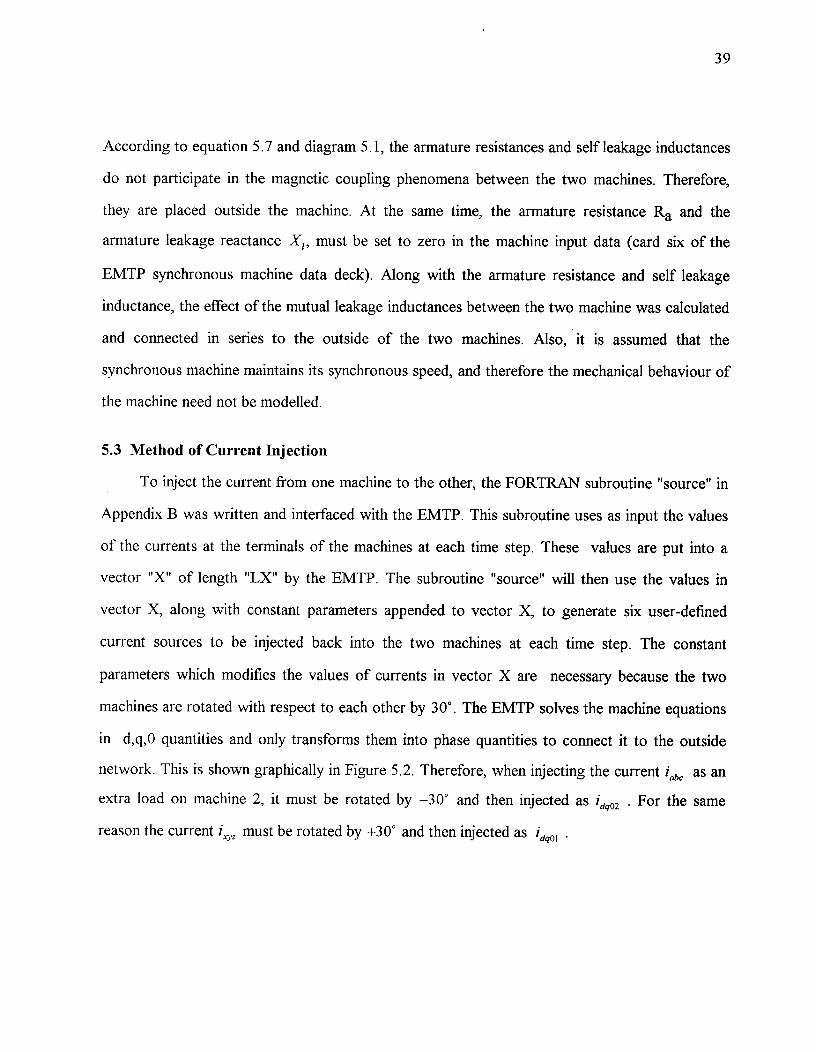
According to equation 5.7 and diagram 5.1, the armature resistances and self leakage inductances

do not participate in the magnetic coupling phenomena between the two machines. Therefore,

they are placed outside the machine. At the same time, the armature resistance R a and the

armature leakage reactance X1 , must be set to zero in the machine input data (card six of the

EMTP synchronous machine data deck). Along with the armature resistance and self leakage

inductance, the effect of the mutual leakage inductances between the two machine was calculated

and connected in series to the outside of the two machines. Also, it is assumed that the

synchronous machine maintains its synchronous speed, and therefore the mechanical behaviour of

the machine need not be modelled.

5.3 Method of Current Injection

To inject the current from one machine to the other, the FORTRAN subroutine "source" in

Appendix B was written and interfaced with the EMTP. This subroutine uses as input the values

of the currents at the terminals of the machines at each time step. These values are put into a

vector "X" of length "LX" by the EMTP. The subroutine "source" will then use the values in

vector X, along with constant parameters appended to vector X, to generate six user-defined

current sources to be injected back into the two machines at each time step. The constant

parameters which modifies the values of currents in vector X are necessary because the two

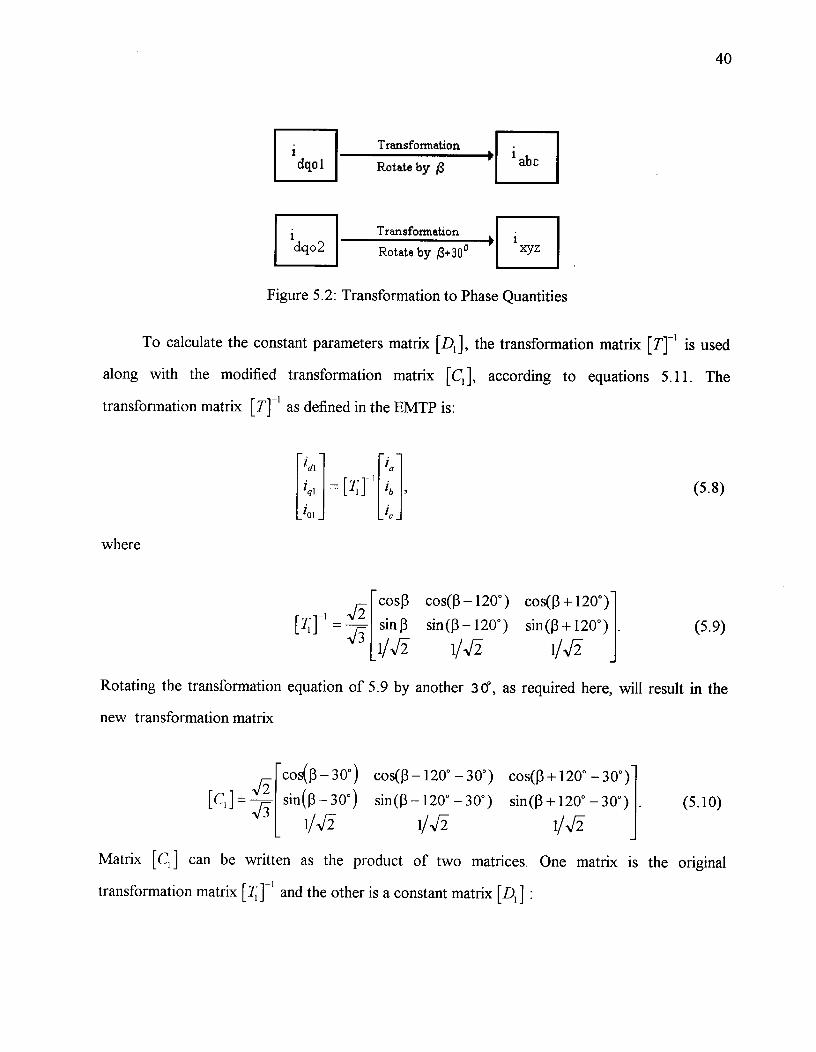
machines are rotated with respect to each other by 30°. The EMTP solves the machine equations

in d,q,0 quantities and only transforms them into phase quantities to connect it to the outside

network. This is shown graphically in Figure 5.2. Therefore, when injecting the current as an

extra load on machine 2, it must be rotated by —30° and then injected as idq02 . For the same

reason the current must be rotated by +30° and then injected as ido, .

1-1

lc_

(5.8)

cosf3^cos((3 -120°) cos((3+120°) -

sin (3^sin ((3 -120°) sin 03 +120°) (5.9)1/Nri^1/-5 1/5

iql

i01

where

[T1] 1 =

40

dqolTransformation i abc0Rotate by 13

Transformationdqo2 Rotate by 13+30 ° xyz

Figure 5.2: Transformation to Phase Quantities

To calculate the constant parameters matrix [DJ, the transformation matrix [T]- ' is used

along with the modified transformation matrix [C I ], according to equations 5.11. The

transformation matrix [7] as defined in the EMTP is:

_ • -'cll.^IQ

Rotating the transformation equation of 5.9 by another 3 0, as required here, will result in the

new transformation matrix

-^,cosQ3 -30°) cos(j3 -120° -30°) cos(3 +120° -30°) -

[C,] = 3 sin ‘ (3 - 30°) sin(13 - 120° -30°) sin03 +120° - 30°)1/5^1/5^1/5

(5.10)

Matrix [Cd can be written as the product of two matrices. One matrix is the original1transformation matrix [7; and the other is a constant matrix [R] :

41

[CI]

[R]= [TIC, ]; and

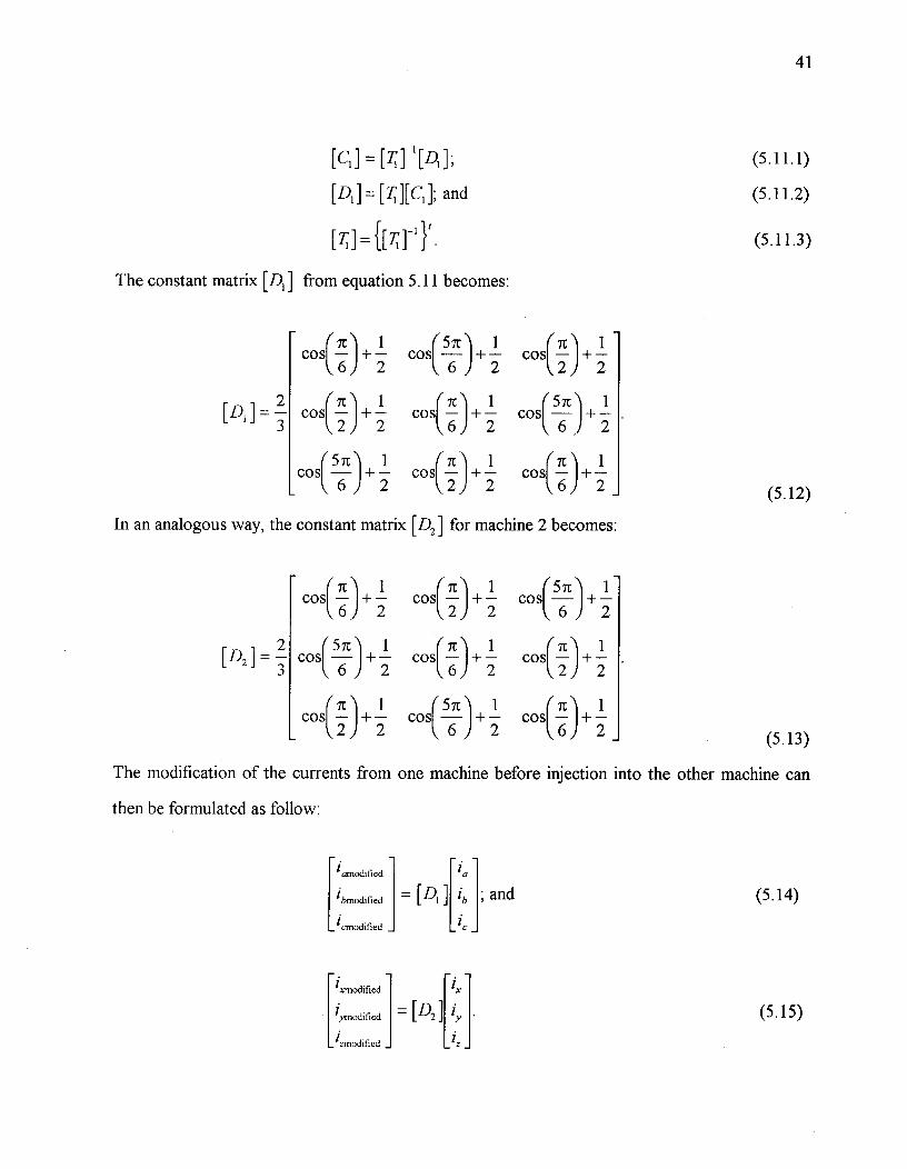
The constant matrix [D1 ] from equation 5.11 becomes:

(5.11.3)

COS( 6

+ 2^6

cos(-51 + 2^2

cos(-71 +-12

(5.12)

In an analogous way, the constant matrix [D 2 ] for machine 2 becomes:

(6^2

+ —1^cos it + —1 cos 57c + —1cos —7t2 2^6^2

[D, 7C(cos—2 2^—6 2

+ —1 cost n + —1 cos(— + —57c) 16^2

57t(cos6 2^—2 2

+ —1 cos 7C)2)+

2 cos( —6 l+ 2n^1)

[D,cos(—

5n ) 21+ — cos it + —1 cos It

6^+

—6 2^2 2

7C ) 1^Sic) 21 ^1cos(—

2 2+ — cos

6(— + — cos( 71 ) +

—6 2 (5.13)

The modification of the currents from one machine before injection into the other machine can

then be formulated as follow:

lamodified la

ibmodified

icmodified _

ixmodified

iymodified

= [4 ]

= [D2

ib

lx

and

_

izmodified _ _iz

(5.14)

(5.15)

This modification is the essential part of subroutine source.

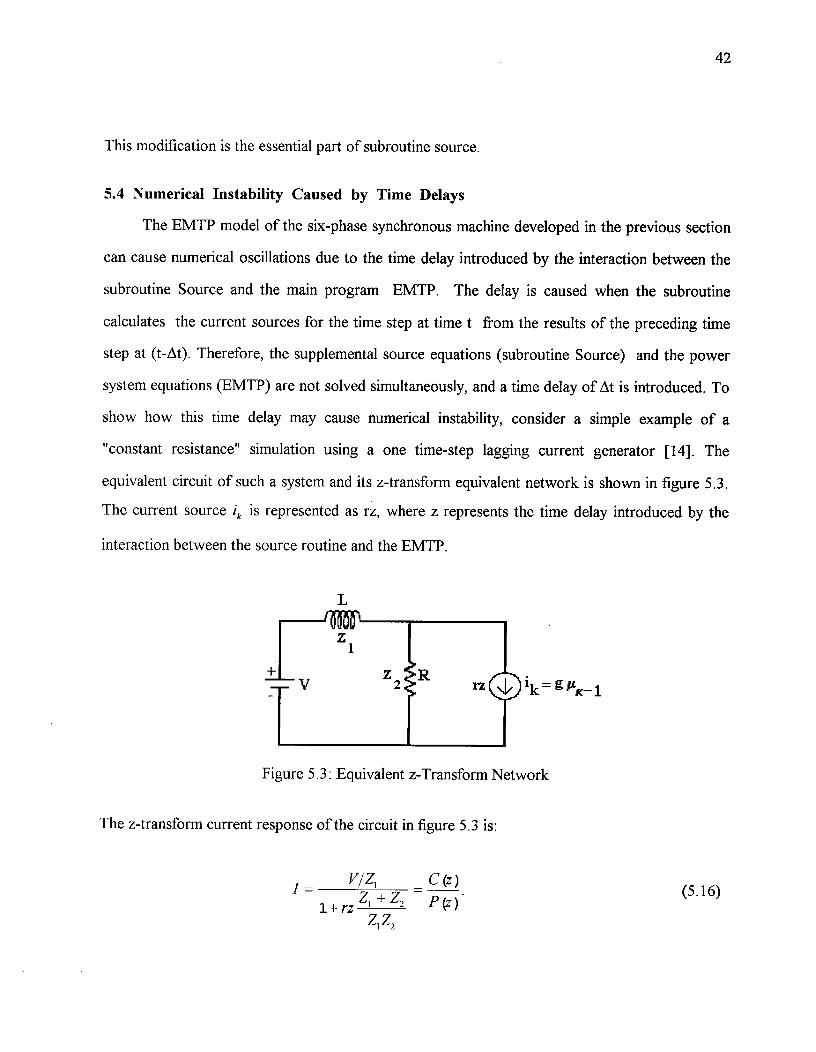
5.4 Numerical Instability Caused by Time Delays

The EMTP model of the six-phase synchronous machine developed in the previous section

can cause numerical oscillations due to the time delay introduced by the interaction between the

subroutine Source and the main program EMTP. The delay is caused when the subroutine

calculates the current sources for the time step at time t from the results of the preceding time

step at (t-At). Therefore, the supplemental source equations (subroutine Source) and the power

system equations (EMTP) are not solved simultaneously, and a time delay of At is introduced. To

show how this time delay may cause numerical instability, consider a simple example of a

"constant resistance" simulation using a one time-step lagging current generator [14]. The

equivalent circuit of such a system and its z-transform equivalent network is shown in figure 5.3.

The current source ik is represented as rz, where z represents the time delay introduced by the

interaction between the source routine and the EMTP.

42

= g AK-1

Figure 5.3: Equivalent z-Transform Network

The z-transform current response of the circuit in figure 5.3 is:

^VIZI ^C (z)I =^, =^Z, i- L^p(z )

^

1+ rz '^2Z, Z,

(5.16)

43

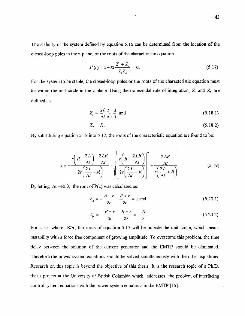
The stability of the system defined by equation 5.16 can be determined from the location of the

closed-loop poles in the z-plane, or the roots of the characteristic equation

P(Z)= ld- rZZ

I 2̂ =0.Zi Z2

(5.17)

For the system to be stable, the closed-loop poles or the roots of the characteristic equation must

lie within the unit circle in the z-plane. Using the trapezoidal rule of integration, Z1 and Z2 are

defined as:

2L z- 1= andAt z + 1

(5.18.1)

Z2 = R .^ (5.18.2)

By substituting equation 5.18 into 5.17, the roots of the characteristic equation are found to be:

r ( R 2 LR) -2^2LR

At)^At riR- 2L)+ 2 LR

At) At

z = (5.19)2r' At +R

At2,-( 2L +R)

Atr(-2L R)•

At

By letting At ->0.0, the root of P(z) was calculated as:

R - r R + rZ a = ^ = 1 and^ (5.20.1)2r^2r

R-r R+r^R(5.20.2)

Zb -^2r^2r

For cases where R>r, the roots of equation 5.17 will be outside the unit circle, which means

instability with a force free component of growing amplitude. To overcome this problem, the time

delay between the solution of the current generator and the EMTP should be eliminated.

Therefore the power system equations should be solved simultaneously with the other equations.

Research on this topic is beyond the objective of this thesis. It is the research topic of a Ph.D.

thesis project at the University of British Columbia which addresses the problem of interfacing

control system equations with the power system equations in the EMTP [15].

44

5.5 Testing the EMTP Model

In order to test the EMTP six-phase synchronous machine model developed in the previous

section , a six-phase short circuit at the terminals of the machine is considered. The results from

this run are then compared against the solution obtained from solving the differential equations

with the fourth order Runge-Kutta method (RK4), as shown in chapter 4. The synchronous

machine model of the EMTP accepts as data input either the transient and subtransient reactances

and time constants, which are then converted to self and mutual impedances, or directly the self

and mutual impedances of the windings. In this thesis, input was in the form of self and mutual

impedances, to insure that the data is identical with that of the Runge-Kutta solution. The

complete EMTP input data listing for modelling the six-phase synchronous machine and the six-

phase short circuit is shown in Appendix C. The numerical simulation with the EMTP has been

carried out from t=Os to t=0.12s, with a step size of 50i,ts. The generator was open circuited

before the fault was applied at time zero. Figure 5.4 shows the comparisons between the EMTP

model and the corresponding solution of the differential equations with the Runge-Kutta method,

for the armature current for the first few cycles, in phase "a" and "x". The EMTP model gives,

practically, the same results than those obtained from chapter 4. The fault current takes a long

time to reach steady state because of the small value of the resistances. Figure 5.5 shows the

comparison of the steady-state short circuit current in phase "a", for the two solution methods.

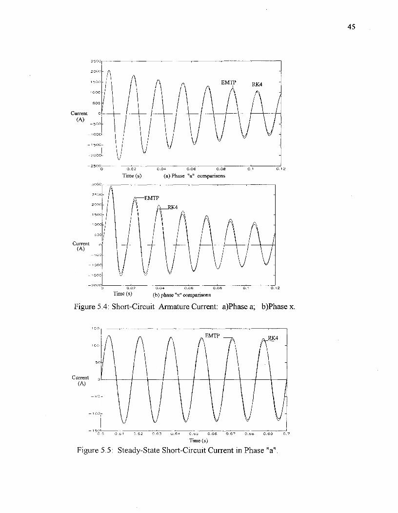
Figure 5.5: Steady-State Short-Circuit Current in Phase "a".

45

3000

2000

1000

Current 0(A)

- 1000

- 2000

- 3000

46

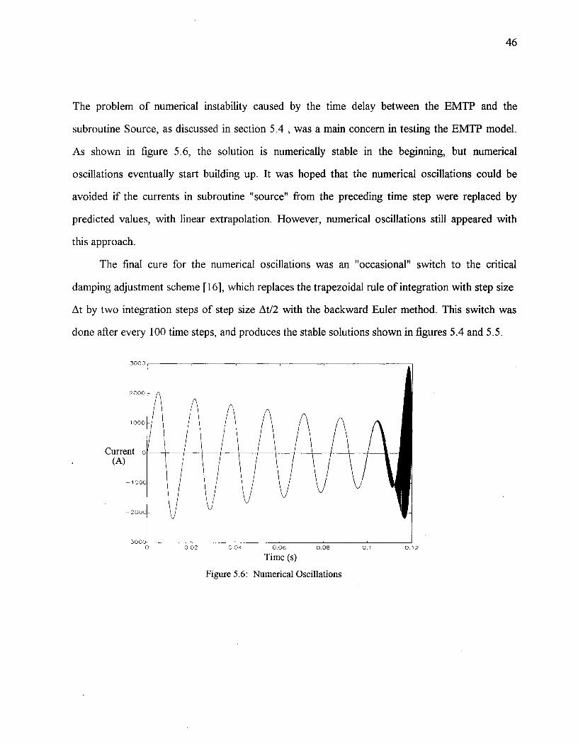
The problem of numerical instability caused by the time delay between the EMTP and the

subroutine Source, as discussed in section 5.4 , was a main concern in testing the EMTP model.

As shown in figure 5.6, the solution is numerically stable in the beginning, but numerical

oscillations eventually start building up. It was hoped that the numerical oscillations could be

avoided if the currents in subroutine "source" from the preceding time step were replaced by

predicted values, with linear extrapolation. However, numerical oscillations still appeared with

this approach.

The final cure for the numerical oscillations was an "occasional" switch to the critical

damping adjustment scheme [16], which replaces the trapezoidal rule of integration with step size

At by two integration steps of step size At/2 with the backward Euler method. This switch was

done after every 100 time steps, and produces the stable solutions shown in figures 5.4 and 5.5.

O^

0.02^0.04^0.06^

0.08^

0.1^

0.12

Time (s)

Figure 5.6: Numerical Oscillations

Chapter 6

CONCLUSIONS

6.1 Results in Thesis

Six-phase synchronous machines are increasingly being used as part of 12-pulse converter-

fed high-power drives. This kind of arrangement, used in power plant auxiliary systems, is very

beneficial for the reduction of harmonic losses and torque pulsations. The aim of this thesis was to

derive a mathematical model for investigating the transient performance of a six-phase

synchronous machine and to develop a model for the simulation of such machines with the EMTP.

The first part of this thesis was devoted to the derivation of the equivalent circuit of a six-

phase synchronous machine with 30° displacements between the two sets of three-phase

windings. This equivalent circuit includes the effects of stator winding mutual leakage coupling

between the two three-phase winding sets. Since the machine inductances are all functions of the

rotor position, Park's coordinate transformation was used to project the rotating fluxes onto the

field axis, where they appear as stationary during steady-state operation. The six-phase machine

reactances and resistances were then derived by relating their values to known three-phase

machine values. These parameters were derived assuming the six-phase machine was constructed

from a three-phase machine by splitting the stator windings into two equal three-phase sets while

retaining the same number of turns per pole.

The transient performance of the six-phase synchronous machine was simulated by solving

the differential equations of the machine, for the case of a six-phase short-circuit at the terminals

of the machine. To solve the ordinary differential equations, the fourth-order Runge-Kutta

method was used. The obtained curves for both, the short-circuit armature currents and the field,

current were consistent with the behaviour of short-circuit currents for three-phase machines

[17] .

47

48

The EMTP model for a six-phase synchronous machine presented in this thesis was based

on the idea of representing the six-phase machine as two three-phase machines in parallel. The

magnetic coupling effect between the two three-phase sets, which was created by currents coming

from both machines, was represented by injecting to the terminals of each machine the current

coming from the other machine. This method of current injection was achieved by adding a

FORTRAN subroutine inside the EMTP source code. This subroutine uses the values of the

currents at the terminals of the machines, and after a phase rotation, generates six user-defined

current sources to be injected back into the two machines at each time step. The test validation of

the proposed EMTP model was carried out by simulating a six-phase sudden short circuit at the

terminals of the machine. The results from this simulation were then compared against the

solution obtained from solving the differential equations with a fourth-order Runge-Kutta method.

The EMTP model gave, practically, the same results as those obtained from solving the

differential equations with the Runge-Kutta method. The results of this comparison confirm the

accuracy of the proposed EMTP model. The problem of numerical oscillations was solved by

using the critical damping adjustment scheme.

6.2 Suggestions for Future Work

In a paper presented at the European EMTP User Group Meeting in October 1992 [18], H.

Knudsen describes an ongoing Ph.D. project, involving the Danish utility company ELKRAFT

and the Technical University of Denmark, on modelling of six-phase synchronous machines with 2

three-phase windings spatially displaced by 30° . In this work the six-phase machine equations

were solved using the "MODELS" input option for control system simulations. With this

approach the results appear in the network modelled by the EMTP in the next time step, as

controlled current sources. Knudsen felt that CDA is needed in the synchronous machine

equations of MODELS to suppress numerical oscillations at time of discontinuities (switch

closing and opening). However, the program version ATP which he uses does not have CDA

49

implementation. There is also the problem of introducing a time delay into the interaction between

the synchronous machine equations in MODELS and the network equations in the EMTP, which

may cause numerical instabilities.

In order to overcome the above limitations, the six-phase synchronous machine equations

should be solved simultaneously with the network. This is possible in UBC's EMTP version

MicroTran with subroutine CONNEC [12], which represents the network as a Thevenin

equivalent circuit, seen from the machine terminals, to the machine equations inside the

subroutine. MicroTran also uses the CDA scheme for the suppression of numerical oscillations,

which is not available in the EMTP version ATP. Implementation of the six-phase machine

equations with the trapezoidal rule of integration, and with the backward Euler method for the

CDA scheme, is a major effort, which was beyond the scope of this thesis.

50

REFERENCES

[1]. Barton T.F., "The Double Winding Generator," General Electric Rev., June 1929, pp.302-308.

[2]. Liyu, C., L. Fahai, Y. Bingshou and G. Jingde, "A Mathematical Model for Converter-FedSynchronous Machines With Dual Three-Phase Windings," International Conference onElectrical Machines, Zurich, Switzerland, August 29, 1991, pp. 347-351.

[3]. Kataoka, Teruo and E.H. Watanabe, "Steady-State Characteristic of a Current-SourceInverter/Double-Wound Synchronous Machine System for Ac Power Supply," IEEETransactions on Industry Applications, Vol. 16, No. 2, 1980, pp. 262-270.

[4]. Park, R.H., "Two-Reaction Theory of Synchronous Machines: Generalized Method ofAnalysis-Part 1," Transactions MEE, Vol. 29, No. 33, 1929, pp. 716-730.

[5]. Schiferl, R.F., "Six Phase Synchronous Machine With AC and DC Stator Connection,"IEEE Transactions on Power Apparatus and Systems, Vol. PAS-102, No.8, August 1983,pp. 2685-2700.

[6]. Bunzel, E. and G. Muller, "General Analysis of a 6-Phase Synchronous Machine,"International Conference on Electrical Machines, Zurich, Switzerland, August 29, 1991,pp. 333-340.

[7]. Fuchs, E.F. and L.T. Rosenberg, "Analysis of Alternator With Two Displaced StatorWindings," IEEE Transactions on Power Apparatus and System, Vol. 93, No. 6, 1974,pp. 1776-1786.

[8]. Moustafa, E., J.P. Chassande and M. Poloujadoff, "A d-q Modelling of A Six-PhaseArmature Synchronous Machine," Paper B6.3, 16th University Power EngineeringConference, Sheffield, England, April 1981.

[9]. Alger, P.L., Induction Machines, 2nd ed., Gordon and Breach Publishers, New York,1970.

[10]. Press, W.H., et. al., Numerical Recipes, Cambridge University Press, New York, 1986.

[11]. Dommel, H.W., "Digital Computer Solution of Electromagnetic Transients in Single andMultiphase Networks," IEEE Trans., Vol. PAS-88, April 1969, pp. 388-399.

51

[12]. Dommel, H.W., Electromagnetic Transients Program Reference Manual (EMTP TheoryBook), Bonneville Power Administration, Portland, U.S.A., August 1986.

[13]. Bompa, L., "EMTP Model for Multiple Coil Synchronous Machines," 14th EMTPEuropean User Group Meeting, Trondheim, Norway, May 1988.

[14]. Lima, J.A., "Numerical Instability Due to EMTP_TACS Inter-relation," EMTPNewsletter, Vol. 5, No. 1, Jan. 1985, pp. 21-33.

[15]. Araujo, A.E.A., H.W. Dommel and J.R. Marti, "Numerical Instabilities in Power SystemTransient Simulations,"^Proceedings of the TASTED International Conference,Vancouver, Canada, August 7, 1992, pp. 176-180.

[16]. Marti, J.R. and Lin-Jiming, "Suppression of Numerical Oscillations in the EMTP," IEEETrans. Power Systems, Vol. 4, May 1989, pp. 739-747.

[17]. Adkins, B. and Harley, R.G., The General Theory of Alternating Current Machines, JohnWiley & Sons, Inc., New York, 1975.

[18]. Knudsen, H., "Implementation of machine model of a 6-phase synchronous machine with2 three-phase windings spatially displaced by 30° using EMTP MODELS," EMTPAutumn Meeting, Heverlee, Belgium, November 9, 1992.

APPENDIX A

Fourth-order Runge-Kutta Procedure

This Appendix shows the FORTRAN listing of the simulation program and its

associated subroutines for the solution of the six-phase synchronous machine current

equations for the case of a six-phase short circuit at the terminals of the machine, as

presented in chapter 4. The FORTRAN program "Solve.for" solves the short-circuit

current equations with the fourth-order Runge-Kutta method, and gives the results as id1 ,

iql and i01 or id2 i92 and i02 . The program "Phasel.for" transforms the d, q and 0

quantities of windings a,b,c into phase quantities. The program "phase2.for" transforms

id2 5 i92 and ice into the phase quantities x, y and z.

PROGRAM SOLVE.FORC This program solves the short-circuit current of the six-phase machine andC gives the result in d, q and 0 quantities for winding a,b,c and x,y,z.C The method used is fourth-order Runge-Kutta.C

PARAMETER(NVAR=9)DIMENSION ISTART(NVAR)EXTERNAL DERIVSREAL*8 XBEGIN,XEND,ISTART,PI,DEITATOPEN(10,FILE='solve 1. OUT',STATUS='UNKNOWN')XBEGIN=0.0D0DELTAT=5.0D-5NSTEP=1600XEND=NSTEP*DELTAT

C ISTART(1) is the initial value of I(1)--x(0)C ISTART(2) is the initial value of I(2)--xdot(0)

ISTART(1)=0.0ISTART(2)=0.0ISTART(3)=0.0

52

ISTART(4)=0.0ISTART(5)=456.35ISTART(6)=0.0ISTART(7)=0.0ISTART(8)=0.0ISTART(9)=0.0CALL RKDUMB(ISTART,NVAR,XBEGIN,XEND,NSTEP,DERIVS)ENDSUBROUTINE DERIVS(T,I,DIDT)DIMENSION I(*),DIDT(*)REAL*8 I,DIDT,TDIDT(1)=-118.6*1(1)+1795.9*1(2)+66.2*1(3)+1415.99(4)+2.49(5)+* 3.2*1(6)+1015.4*I(7)-1101.3DIDT(2)=-2110.8*1(1)-106.69(2)-1736.8*1(3)+76.99(4)-1251.4*1(5)* -1251.4*1(6)+3.5*I(7)+0.0DIDT(3)=66.2*I(1)+1415.9*1(2)-118.6*1(3)+1795.9*1(4)+2.4*1(5)+* 3.2*1(6)+1015.4*1(7)-1101.3DIDT(4)=-1736.8*1(1)+76.99(2)-2110.8*1(3)-106.69(4)-1251.4*1(5)* -1251.4*1(6)+3.5*I(7)+0.0DIDT(5)=40.3*1(1)-2471.5*1(2)+40.39(3)-2471.5*I(4)-10.09(5)+* 3.8*I(6)-1562.8*1(7)+4552.1DIDT(6)=35.8*1(1)-2191.7*1(2)+35.89(3)-2191.7*1(4)+2.6*1(5)-* 13.5*1(6)-1385.8*I(7)-1166.1DIDT(7)=4825.2*1(1)+37.3*I(2)+4825.2*1(3)+37.3*1(4)+3138.8*1(5)+* 3138.8*I(6)-11.0*1(7)+0.0DIDT(8)=-8055.55*I(8)DIDT(9)=-8055.55*I(9)RETURNEND

SUBROUTINE RKDUMB(ISTART,NVAR,X1,X2,NSTEP,DERIVS)PARAMETER (NMAX=10)INTEGER CONTREAL*8 ISTART,V,DV,X1,X2,H,XDIMENSION ISTART(NVAR),V(NMAX),DV(NMAX)DO 11 I=1,NVAR

V(I)=ISTART(I)11 CONTINUE

X=X1H=(X2-X1)/NSTEPCONT=0WRITE(10,100) X1,V(1),V(2),V(8)

C WRITE(10,100) X1,V(3),V(4),V(9)

53

DO 13 K=1,NSTEPCALL DERIVS(X,V,DV)CALL RK4(V,DV,NVAR,X,H,V,DERIVS)

WRITE(10,100) X,V(1),V(2),V(8)C WRITE(10,100)X, V(3), V(4), V(9)

IF(X+H.EQ.X)PAUSE 'Stepsize not significant in RKDUMB.'X=X+H

13 CONTINUE100 FORMAT(F16.6,2X,F10.4,2X,F10.4,2X,F10.4)

RETURNEND

SUBROUTINE RK4(Y,DYDX,N,X,H,YOUT,DERIVS)PARAMETER (NMAX=10)REAL*8 Y,DYDX,YOUT,YT,DYT,DYM,X,H,H6,BH,XHDIMENSIONY(N),DYDX(N),YOUT(N),YT(NMAX),DYT(NMAX),DYM(NMAX)HH=H*0.5H6=H/6.XH=X+HHDO 11 I=1,N

YT(I)=Y(I)+HH*DYDX(I)11 CONTINUE

CALL DERIVS(XH,YT,DYT)DO 12 I=1,N

YT(I)=Y(I)+HH*DYT(I)12 CONTINUE

CALL DERIVS(XH,YT,DYM)DO .13 I=1,N

YT(I)=Y(I)+H*DYM(I)DYM(I)=DYT(I)+DYM(I)

13 CONTINUECALL DERIVS(X+H,YT,DYT)DO 14 I=1,N

YOUT(I)=Y(I)+H6*(DYDX(I)+DYT(I)+2. *DYM(I))14 CONTINUE

RETURNEND

PROGRAM PHASEl.FORC This program transforms the d, q and 0 (1) quantities intoC phase quantities a, b and c.

DIMENSION TINV(3,3),X(3),Y(3)

54

REAL*8 BETA,LAMDA,TIME,TINV,OMEGA,X,PI,YOPEN(12,FILE='PHASE1.OUT',STATUS='UNKNOWN')OPEN(10,FILE= 1 SOLVE1.OUT',STATUS='OLD')PI=DACOS(-1.0D0)WRITE(*, *) 'OMEGA,LAMDA'READ(*,*) OMEGA,LAMDA

300 READ(10,*,END=200) TIME,X(1),X(2),X(3)BETA=OMEGA*TIME+LAMDATINV(1,1)=DSQRT(2.D0)/DSQRT(3.D0)*DCOS(BETA)TINV(1,2)=DSQRT(2.D0)/DSQRT(3.D0)*DSIN(BETA)TINV(1,3)=1/DSQRT(3.D0)TINV(2, 1)=D S QRT(2 . DO)/D S QRT(3 .D0)*DCO S(BETA-2. DO*PI/3 .D0)TINV(2,2)=DSQRT(2.D0)/DSQRT(3.D0)*DSIN(BETA-2.D0*PI/3.D0)TINV(2,3)=1/DSQRT(3.D0)TINV(3, 1)=D S QRT(2 . DO)/D SQRT(3 . DO)*DCO S(BETA+2 DO*PI/3 .D0)TINV(3,2)=DSQRT(2.D0)/DSQRT(3.D0)*DSIN(BETA+2.D0*PI/3.D0)TINV(3,3)=1/DSQRT(3.D0)CALL MULTVECTOR(TINV,X,Y)WRITE(12,100) TIME,Y(1),Y(2),Y(3)

100 FORMAT(F16.6,2X,F16.4,2X,F16.4,2X,F16.4)GO TO 300

200 CONTINUEEND

SUBROUTINE MULTVECTOR(A,X,Y)DIMENSION A(3,3),X(3),Y(3)REAL*8 A,X,SUM,YDO 1 I=1,3SUM=0.D0DO 2 K=1,3SUM=SUM+A(I,K)*X(K)

2 CONTINUEY(I)=SUM

1 CONTINUERETURNEND

PROGRAM PHASE2.FORC This program transforms the d, q, and 0 (2) quantities intoC the phase quantities x, y and z.

DIMENSION TINV(3,3),X(3),Y(3)REAL*8 BETA,LAMDA,TIME,TINV,OMEGA,X,PLYOPEN(12,FILE—'phase2.0UT',STATUS='UNKNOWN')

55

OPEN(10,FILE-2solve2. out', S TATUS='OLD')PI=DACOS(-1.0D0)WRITE(*, *) 'OMEGA,LAMDA'READ (*, *) OMEGA,LAMDA

300 READ(10, *,END=200) TIME, X(1), X(2), X(3)BETA=OMEGA* TIME+LAMDATINV(1, 1)=D S QRT(2. DO)/D SQRT(3 .D0)*DCO S(BETA-PI/6.D0)TINV(1,2)=DSQRT(2.D0)/DSQRT(3.D0)*DSIN(BETA-PI/6.D0)TINV(1,3)=1/D S QRT(3 .D0)TINV(2, 1)=D S QRT(2. DO)/D SQRT(3 .D0)*DCOS(BETA-5.DO*PI/6.D0)TINV(2,2)=DSQRT(2.D0)/DSQRT(3.D0)*DSIN(BETA-5.D0*PI/6.D0)TINV(2,3)=1/D S QRT(3 .D0)TINV(3, 1)=D SQRT(2 . DO)/D SQRT(3 .D0)*DCO S(BETA+5 DO*PU6. DO)TINV(3,2)=DSQRT(2.D0)/DSQRT(3.D0)*DSIN(BETA+5.D0*PI/6.D0)TINV(3 ,3)=1/D S QRT(3 .D0)CALL MULTVECTOR(TINV,X,Y)WRITE(12,100) TIME, Y(1), Y(2), Y(3)

100 FORMAT(F16.6,2X,F16.4,2X,F16.4,2X,F16.4)GO TO 300

200 CONTINUEEND

SUBROUTINE MULTVEC TOR(A, X, Y)DIMENSION A(3 ,3), X(3), Y(3 )REAL*8 A, X, SUM, YDO 1 I=1,3SUM=0.D0DO 2 K=1,3SUM= SUM+A(I,K) * X(K)

2 CONTINUEY(I)=SUM

1 CONTINUERETURNEND

56

APPENDIX B

Subroutine Source

This Appendix shows the FORTRAN listing of the subroutine Source. This

subroutine uses as input the values of the currents at the terminals of the two machines at

each time step. The current values are generated by EMTP and stored in x(1) to x(6). The

subroutine then uses these values, along with the constant parameters x(7) to x(9) needed

for the definition of [D, and [D2 ], to generate six user-defined current sources to be

injected back into the network at each time step. This subroutine also uses a linear

extrapolation, to reduced the severity of the time delay between the EMTP and the

subroutine Source.

PROGRAM SOURCE.FORSUBROUTINE SOURCE(X,LX,SOURC,T,DELTAT,IHALF,KREAD)DIMENSION X(*), SOURC(*),AUX1 (1 0)IMPLICIT REAL*8 (A-H 2 O-Z),INTEGER*4 (I-N)SAVE AUX1KREAD=OSOURC(1)=X(1)*X(7)+X(2)*X(8)+X(3)*X(9)SOURC (2)=X( 1 )*X(9)+X(2)*X(7)+X(3 )*X(8)S OURC (3 )=X( 1 )*X(8)+X(2)*X(9)+X(3 )*X(7)SOURC(4)=X(4)*X(7)+X(5)*X(9)+X(6)*X(8)SOURC(5)=X(4)*X(8)+X(5)*X(7)+X(6)*X(9)SOURC(6)=X(4) *X(9)+X(5)*X(8)+X(6)*X(7)

C

^

^Linear Extrapolation for improving the time delay.IF(X(10).EQ.0.0D0) RETURNIF(T.EQ.0.0D0) THENDO 15 I=1,6

AUX 1 (I)=S OURC(I)15 CONTINUE

END IF

57

DO 20 I=1,6AUX2=2.DO*SOURC(I)-AUX1(I)AUX1(I)=S OURC (I)SOURC(I)=AUX2

20 CONTINUEEND

58

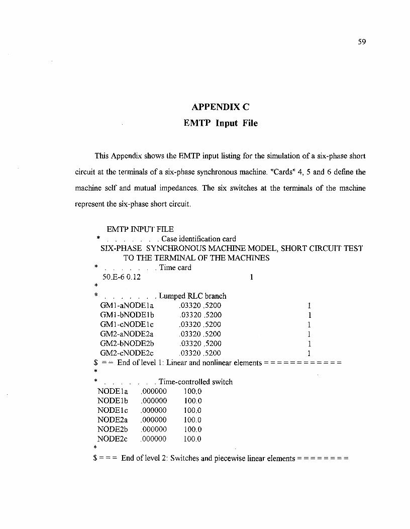
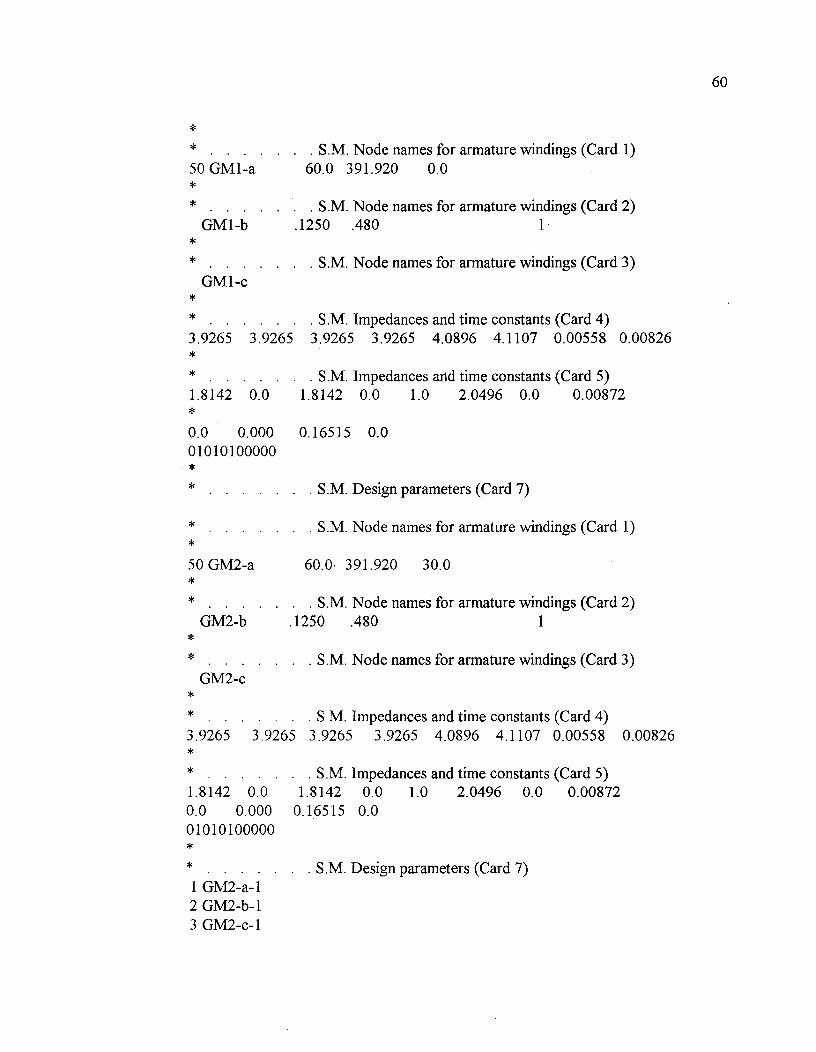
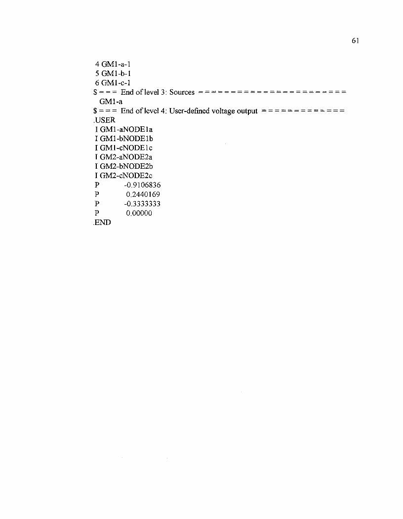
APPENDIX C

EMTP Input File

This Appendix shows the EMTP input listing for the simulation of a six-phase short

circuit at the terminals of a six-phase synchronous machine. "Cards" 4, 5 and 6 define the

machine self and mutual impedances. The six switches at the terminals of the machine

represent the six-phase short circuit.

EMTP INPUT FILE^ Case identification card

SIX-PHASE SYNCHRONOUS MACHINE MODEL, SHORT CIRCUIT TESTTO THE TERMINAL OF THE MACHINES^ Time card

50.E-6 0.12** ^ Lumped RLC branch

1

GM1-aNODEla .03320 .5200 1GM1-bNODE1b .03320 .5200 1GM1-cNODElc .03320 .5200 1GM2-aNODE2a .03320 .5200 1GM2-bNODE2b .03320 .5200 1GM2-cNODE2c .03320 .5200 1

$ = = End of level* 1: Linear and nonlinear elements

Time-controlled switchNODEla .000000 100.0NODElb .000000 100.0NODElc .000000 100.0NODE2a .000000 100.0NODE2b .000000 100.0NODE2c .000000 100.0*

$ = = = End of level 2: Switches and piecewise linear elements

59

S M̂ Design parameters (Card 7)

S M^Node names for armature windings (Card 1)

60.0. 391.920^30.0

S M^Node names for armature windings (Card 2)GM2-b^.1250^.480^1

**50 GM2-a**

**

S M̂ Node names for armature windings (Card 1)

50 GM1-a^60.0 391.920^0.0*S M Node names for armature windings (Card 2)

GM1-b^.1250 .480^1*S M Node names for armature windings (Card 3)

GM1-c*S M Impedances and time constants (Card 4)

3.9265 3.9265 3.9265 3.9265 4.0896 4.1107 0.00558 0.00826*S M Impedances and time constants (Card 5)

1.8142 0.0^1.8142 0.0^1.0^2.0496 0.0^0.00872*0.0^0.000^0.16515 0.001010100000*

60

*^S M^Node names for armature windings (Card 3)

GM2-c*^S M^Impedances and time constants (Card 4)

3.9265^3.9265 3.9265 3.9265 4.0896 4.1107 0.00558 0.00826*^S M^Impedances and time constants (Card 5)

1.8142 0.0^1.8142^0.0^1.0^2.0496^0.0^0.00872

^

0.0^0.000^0.16515^0.001010100000*

^S M^Design parameters (Card 7)1 GM2-a-12 GM2-b-13 GM2-c-1

4 GM1-a-15 GM1-b-16 GM1-c-1$ = = = End of level 3: Sources ^

GM1-a$ = = = End of level 4: User-defined voltage output.USERI GM1-aNODElaI GM1-bNODElbI GM1-cNODElcI GM2-aNODE2aI GM2-bNODE2bI GM2-cNODE2cP -0.9106836P 0.2440169P -0.3333333P 0.00000.END

61