Adaptive finite element analysis of structures under transient dynamic loading using modal...

Finite Elements in Analysis and Design 31 (1999) 255—272

Adaptive finite element analysis of structures under transientdynamic loading using modal superposition

A. Dutta!, C.V. Ramakrishnan",*, P. Mahajan"

! Regional Engineering College, Silchar 788010, India" Applied Mechanics Department, Indian Institute of Technology, Delhi 110016, India

Abstract

In this paper, the error estimation and adaptive strategy developed for the linear elastodynamic problem undertransient dynamic loading based on the Z—Z criterion is utilized for 2D and plate bending problems. An automatic meshgenerator based on “growth meshing” is utilized effectively for adaptive mesh refinement. Optimal meshes are obtainediteratively corresponding to the prescribed domain discretization error limit and for a chosen number of basis modessatisfying modal truncation errors. Numerous examples show the effectiveness of the integrated approach in achievingthe target accuracy in finite element transient dynamic analysis. ( 1999 Elsevier Science B.V. All rights reserved.

Keywords: Finite element; Adaptive; Error estimation; Mesh generation; Stress recovery

1. Introduction

Estimates of errors and adaptive analyses of practical finite element problems are subjects ofgreat importance if confidence in results is needed for engineering applications. Without theassessment of the reliability of the results it is hardly reasonable to use numerical methods like thefinite element method in such safety-sensitive areas as shape optimization of machine parts,construction of aeroplanes or dimensioning of nuclear power plants. Therefore, the a posteriorierror estimation is now considered to be nearly as important as the finite element analysis itself.

Using finite elements, the linear dynamic transient response is usually solved either by modesuperposition or by direct integration schemes. The direct integration method is very highly usefulfor solving nonlinear problems. Procedures describing adaptive time stepping are available in [1,2]and also spatial mesh adaptation [3]. Wiberg and Li [4] have proposed a postprocessed type ofa posteriori estimates in space and also in time when direct integration is used for dynamic

*Corresponding author.

0168-874X/99/$ — see front matter ( 1999 Elsevier Science B.V. All rights reservedPII: S 0 1 6 8 - 8 7 4 X ( 9 8 ) 0 0 0 6 1 - 4

response evaluation. It updates the spatial mesh and time step so that the discretization errors arecontrolled. This process is not only time consuming but also gives rise to new errors as nodal valuesneed to be interpolated from the previous mesh to the newly generated mesh whenever a mesh ischanged. But for large structural problems involving a large time domain, the mode superpositionis widely used. The accuracy obtained by the mode superposition is usually dominated by theaccuracy of the orthogonal modes being used and proper representation of spatially distributedloads by the number of modes selected for the modal analysis. Thus, we find that the followingerrors are introduced. These are (a) domain discretization error, (b) modal truncation error, (c)numerical error in eigen modes and eigen values, and (d) truncation error in numerical integration.While a proper value of time step eliminates truncation error in numerical integration to a greatextent and an appropriate tolerance limit evaluates eigenmodes and eigenvalues accurately,domain discretization error and modal truncation error need elaborate study.

The work reported so far on discretization error estimation under dynamic loading and using themodal superposition scheme are very few. Wilson and Joo [5] have arrived at the final mesh usingRitz vector as the basis of transformation. In their investigation, the authors have made use ofmodal participation and amplification factors and obtained error estimates based on Babuska’scriterion using amplified Ritz modes. This procedure is a bit cumbersome and does not givea measure of the actual error in the transient response. Cook and Avrashi [6] have discussed theprocedure for estimating the discretization error of the finite element modelling as applied to thecalculation of natural frequency of vibrations. Meshes are obtained corresponding to each mode.Dutta and Ramakrishnan [7] proposed a measure for discretization which is a logical extension ofZienkiewicz and Zhu’s [8] error criterion by involving time integration to consider the variation ofresponse with time. Using this error measure, an adaptive mesh refinement strategy is proposedwhich yields good control over the discretization errors in transient dynamic analysis. An optimalmesh is achieved iteratively wherein meshes are refined on the basis of error indicators so that thediscretization errors are within the prescribed limit for a chosen number of basis modes satisfyingthe modal cut-off criteria, when the modal superposition method is used.

In this paper, we have adopted the adaptive strategy given by Dutta and Ramakrishnan [7] forarriving at an optimal mesh for a prescribed domain discretization error limit and for a chosennumber of basis modes satisfying modal cut-off criteria for accurate evaluation of response undertransient dynamic loading. A 2-D quadrilateral automatic mesh generator [9] is used for carryingout adaptive refinement of the finite element mesh. The adaptive strategy is extended to estimationof errors and adaptive analysis for plates and shells where the well-known degenerate shell elementby Ahmad et al. [10] is ued for evaluation of response under dynamic loads.

2. Error measure for domain discretization

The dynamic response of a linear structural dynamic system that is subjected to general dynamicloads is given

Mz(#Kz#Cz"q(t). (1)

The initial conditions are z(0)"z0

and z(0)"z0.

256 A. Dutta et al. /Finite Elements in Analysis and Design 31 (1999) 255—272

Here

z is the vector of nodal displacements,

M is assembled consistent mass matrix"+ne/1

M(e) where n is the number of elements,

K is assembled stiffness matrix"n+e/1

K(e),

C is assembled damping matrix"+ne/1

C(e), (2)

q(t) is external excitation (time dependent).

FE stresses are calculated as

p"DBz, (3)

where D is the elasticity matrix and B is the strain displacement matrix.The approximate solution p containing discretization errors differs from the accurate solution

pH and the difference is the error ep.Thus,

ep"pH!p, (4)

Zienkiewicz and Zhu [8] suggested a simple approach to get better approximation of p by usinga projection tecnique or nodal averaging procedure. In the projection technique, the use ofweighted residual requirement for equality between pH and p leads to the computation of anaccurate solution of pH which is identical to the least-squares smoothing technique of Hinton andCampbell [11]. Nodal averaging, though very simple, gives very good convergence for most of theproblems. A recent and elegant technique of better stress recovery is done using superconvergentpatch recovery method by Zienkiewicz and Zhu [12]. In the recovery process, it is assumed that theaccurate nodal values pN H belong to a polynomial expansion pH

eof the same complete order ‘p’ as

that present in the basis function N and which is valid over an element patch surroundingthe particular assembly node considered. Such a ‘patch’ represents a union of elements containingthis vertex node (Fig. 1). This polynomial expansion will be used for each component of pH

eand

we get

pHe"Pa, (5)

where P contains the appropriate polynomial terms and a is a set of unknown parameters. Fora general plate and shell problem, the polynomial can be expressed as a function of x, y and z.However, since only plate problems are solved in this paper, x and y are considered only as theparameters in the polynomial expression. Thus, it can be written as

P"[1,x, y,x2,2] (6)

and

a"[a1, a

2, a

3, a

4,2]T. (7)

The determination of the unknown parameters a of the expression given in Eq. (5) is best made byensuring a least-squares fit of this to the set of superconvergent points existing in the patch

A. Dutta et al. /Finite Elements in Analysis and Design 31 (1999) 255—272 257

Fig. 1. Computation of superconvergent nodal values: (n) Gauss point, (v) nodal values determined by recoveryprocedure, (() patch assembly point.

considered. To do this we minimize

F(a)"n+i/1

(pe(x

i, y

i)!pH

e(x

i, y

i))2

"

n+i/1

(pe(x

i, y

i)!P(x

i, y

i)a)2, (8)

where (xi, y

i) are the coordinates of a group of sampling points, n"mk is the total number of

sampling points and k is the number of the sampling points on each element mj(m

j"1,2,2,m) of

the element patch. The minimization condition of F(a) implies that a satisfies

n+i/1

PT(xi, y

i)P(x

i, y

i)a"

n+i/1

PT(xi, y

i)p

e(x

i, y

i). (9)

This can be solved in matrix form as

a"A~1b, (10)

where

A"

n+i/1

PT(xi, y

i)P(x

i, y

i) and b"

n+i/1

PT(xi, y

i)p

e(x

i, y

i). (11)

Once the parameters a are determined, the recovered nodal values of pN H are simply calculated byinsertion of appropriate coordinates into the expression for pH

e. The stresses in the nodes inside the

patch are evaluated using a from Eq. (5). The stresses at boundary nodes can be determined usinginterior patches.


For the time-dependent problem, we propose

g"Ee E

!7Eu E

!7

]100%, (12)

where g is the overall discretization error with

EeE!7"

:T0EeE dt¹

. (13)

The integration is carried out numerically using Simpson’s rule. Also

EuE!7"

:T0EuEdt¹

(14)

where ¹ is the duration of response, EeE is the ‘energy norm’ of the error for the whole domain

EeE"Cn+i/1

EeE2i D

1@2, (15)

where

EeEi"CPX

eTpD~1ep dXD1@2

, (16)

the energy norm of the error in the element i,

EuE"xEuM E2#EeE2y1@2, (17)

where

EuM E"Cn+i/1

EuM E2i D

1@2

and

EuM Ei"CPX

pTD~1pdXD1@2

, (18)

the energy norm of the FE solution.The complete procedure of discretization error measure is given below in an algorithmic form:Table 1

3. Estimation of error due to modal truncation

Modal truncation errors are introduced in the response calculation because of the introductionof a reduced system. Since for a specified number of modes, discretization errors have now beenquantified and an appropriate mesh satisfying the prescribed tolerance limit of gN can be properlydesigned, the measure for control of error due to modal truncation can be carried out effectively.Inclusion of higher modes alone without taking care of domain discretization error leads to


Table 1Algorithm for domain discretization error

(1) Solve MVX"KVwhere V is a matrix of eigen vectors and X is matrix of eigenvalues(2) Calculate dynamic response for t"0,¹M(2.1) For i"1, m nos. of eigenvector solve

M yi(t)"

1

u*$

:t0

fi(q)e~fiui(t~q) sinu

*$(t!q) dq

z(t)"+�

iyi(t)N

where ui$

is the ith damped natural frequency, fiis the damping ratio corresponding to mode

i and fiis the load vector corresponding to mode i and can be written as f

i"�T

iq(t).

(2.2) for e"1, n elementsM Retrieve ze

(t)from z

(t)where z

e(t)is the displacement vector corresponding to the element level

for j"1, number of Gaussian pointM calculate p(j)

e(t)"DB(j)ze

(t)calculate smooth stress pH(j)

e(t)N

Nfor e"1, n elements

M for j"1, number of Gaussian pointM e(j)pe

(t)"pH(j)

e(t)!p(j)

e(t)

EeEe(t)"C:X(e(j)pe

(t))TD~1e e(j)pe

(t)dXD

1@2

EuM Ee(t)"C:X(p(j)pe

(t))TD~1e p(j)pe

(t)dXD

1@2

Nfor the whole strutureEeE

(t)"[+EeE2

e(t)]1@2

EuM E(t)"[+EuM E2

e(t)]1@2N

N(3) Overall domain discretization error

EeE!7"

:T0EeE

(t)dt

¹

EuE!7"

:T0EuE

(t)dt

¹

EuE(t)"xEuM E2

(t)#EeE2

(t)y1@2

g"EeE

!7EuE

!7

]100%

(4) Discretization error at element levelFor i"1, n elements

M mi"

EeEi(t)

eNm

is a refinement indicator at element level


Table 1Continued

where

eNm"gN C

EuM E2(t)#EeE2

(t)n D

1@2

is the allowable element errorg is the permissible overall discretization error

m@i"

:T0midt

¹

If g)gN andIf m@

i(1 for i"1, n STOP

Else hi/%8

"

hi0-$

(m@i)1@p1

hi0-$

is the size of element i of the previous mesh,hi/%8

is the size of element i of the new meshEndifNGo to step 1

erroneous results [7], since there is no guarantee that the chosen mesh is suitable for the inclusionof higher modes. Given a finite element mesh, it is possible to control the modal truncation errors infinite element analysis using the ratios of MPF, modal participation factor and its maximum value(MPF

.!9) and MSF, modal significance factor and its maximum value (MSF

.!9) as demonstrated

by Dutta and Ramakrishnan [7]. The modal participation factor for the ith mode can be written as�T*p/u2

i. The ratio of MPF and MPF

.!9is b

1.and b

1.(d where d is the permissible limit. The

modal significance factor for the ith mode can be written as

�T*p

u2i

]1

J(1!b2i)2#2f

ibi)2

where bi"

uNu

i

and u is the exciting frequency and the ratio of MSF and MSF.!9

is b4.(d.

4. Automated meshing algorithm

A general formulation developed by Sinha and Ramakrishnan [9], termed ‘growth meshing’which is characterized by rule based local selection of elements resulting in an inward propagationof the mesh and includes several existing methods of unstructured gridding, is utilized for adaptiverefinement of the domain. The 2-D quadrilateral meshes are generated mainly following thestrategy adopted by Zhu et al. [13], where two triangles which share a common side are combined.The main feature of the quadrilateral generation is that first two triangles which have a commonside are generated and then the triangles are combined to form a quadrilateral. The process


continues until the domain is fully covered by non-overlapping quadrilaterals. Furthermore, it isrule driven and offers flexibility through the incorporated constraints along with the possibility ofadaptive modification. It is very effective in achieving a rapid gradation effect over irregular andcomplicated domains. However, one drawback of this type of quadrilateral generation by combin-ing triangles is that the quality of the raw quadrilateral mesh produced is usually not goodand mesh quality enhancement procedures are adopted following Zhu et al. [13] and Lee andLo [14].

In order to capture the rapid variation of element size which commonly occurs in adaptiverefinement meshes, the mesh generator employs the previous quadrilateral mesh as the backgroundmesh. Nodal spacing values of the previous mesh obtained through error estimation is utilized forcalculating node spacing at a point of the new mesh to be generated. The nodal spacing at a point iscalculated as [15]

d"+n

i/1(1/r2

i)d

i+n

i/11/r2

i

, (19)

where riis the distance between the node to be generated and the nodal point of the previous mesh,

diis the nodal spacing at the nodal point of the previous mesh and ‘n’ is the total number of nodes.

The nodal points of the previous mesh which are neighbouring close to the point under considera-tion influence in arriving at the value of the nodal spacing at that point. For the generation of anentire quadrilateral element mesh over the domain, the boundary of the domain is transformed intoa polygon with an even number of sides. A set of uniformly distributed sample points is first placedalong the boundary line and node spacing on each sample point is calculated by interpolating itsvalue obtained from the background mesh. The boundary nodes are then generated followinga simple formula given by Lo [16] which allows the position of the new nodes to be calculated oneby one along the boundary. The interior nodes are generated following the strategy given byPeraire et al. [17]. Starting from an active front chosen from the boundary segments, the nodalspacing values at the background mesh are utilized such that the elements with acceptable aspectratio and minimum distortion are generated.

5. Computation of optimal mesh using modal superposition

An overall strategy for accurate computation of dynamic response is given by Dutta andRamakrishnan [7] for plane stress/plane strain problems. Following the same strategy, the numberof basis modes are first obtained for a coarse mesh to begin with, which will satisfy the cut-offcriteria based on b

1.pd or b

4.pd adopted. Discretization errors at element level m@

i(i"1, number

of elements) are determined for those number of modes. Average nodal spacing values arecalculated using m@

ivalues and mesh is then adaptively refined based on those nodal spacing values.

The number of modes required for the refined mesh are determined satisfying the modal cut-offcriteria. The overall domain discretization error g and the discretization error at element level m@

iare

determined for chosen number of modes. Iteration is carried out until the mesh is an optimal onesatisfying the prescribed domain discretization error limit gN corresponding to the number of modeschosen on b

1.or b

4.limit.


5.1. Numerical example

A number of plane stress and plate bending problems have been solved to demonstrate theadaptive strategy and use of the automatic mesh generator in obtaining the optimal meshes.

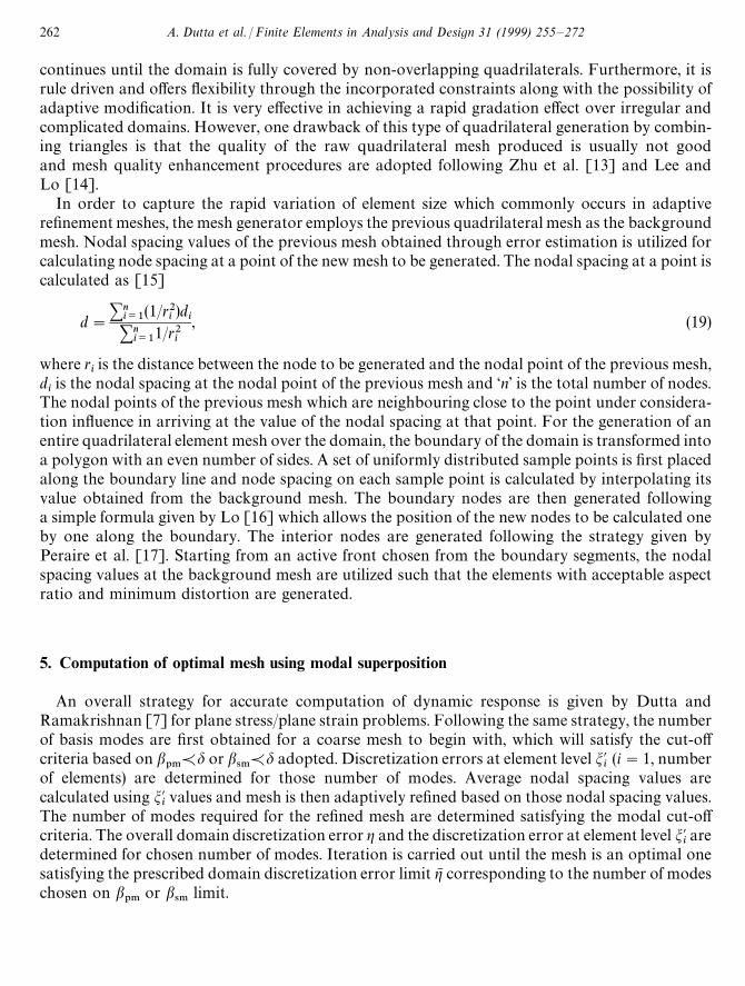
Example 1 (Plane stress plate with a hole). A square plane stress plate with a central holesubjected to harmonic loading of exciting frequency uN "5 rad/s is considered. Because of sym-metry, only a quadrant could be considered for analysis and Fig. 2a is assumed as the startingmesh. The limits of MSF ratios and MPF ratios are chosen as 5e-2. The limit of domaindiscretization error gN is considered as 1%. The geometric and material properties of the plate are asbelow.

Plate: 100 in]100 in]1 in with a central hole of radius of 5, E"0.3e5 lbf/in2, l"0.3;o"1.0 lbm/in2.

For the problem with uN "5 rad/s, 15 eigenmodes are selected to satisfy the modal cut-off criteriacorresponding to the initial mesh (Fig. 2a). The final mesh is obtained after one iteration. Theautomatic mesh generator described earlier is used for adaptive refinement. The exciting frequencyis very low for this example and lies between first and second natural frequencies. The results arepresented in Table 2. The final mesh is shown in Fig. 2b. NIGEN is the number of eigenmodes.

A similar exercise is repeated with exciting frequency uN "25 rad/s and Fig. 3a is assumed as thestarting mesh.

The problem with higher exciting frequency uN "25 rad/s requires 19 basis modes correspondingto the initial mesh (Fig. 3a) in order to satisfy the modal cut-off requirement of b

1.and b

4.p5.e-2.

Fig. 2. Plane stress plate subjected to harmonic loading (u"5): (a) Mesh 1, 12 elements, g"5.38%; (b) Mesh 2, 127elements, g"1.12%.


Table 2Optimal mesh for the problem of a plate with a hole subjected to harmonic loading of uN "5 rad/s

Mesh Limit of NIGEN g (%)b1.

& b4.

Fig. 2a 5.e-2 15 5.383Fig. 2a 5.e-2 17 1.122

Fig. 3. Plane stress plate subjected to harmonic loading (u"25): (a) Mesh 1, 12 elements, g"17.84%; (b) Mesh 2, 348elements, g"2.04%; (c) Mesh 3, 393 elements, g"1.07%.


Table 3Optimal mesh for the problem of a plate with a hole subjected to harmonic loading of uN "25 rad/s

Mesh Limit of NIGEN g (%)b1.

& b4.

Fig. 3a 5.e-2 19 17.842Fig. 3b 5.e-2 23 2.037Fig. 3c 5.e-2 25 1.075

The final mesh is obtained after two iterations and results are shown in Table 3. The excitingfrequency lies between the seventh and eighth natural frequency. The final mesh (Fig. 3c) corre-sponding to this problem is quite different from the one (Fig. 3b) corresponding to uN "5 rad/sbecause of the integration of different numbers of basis modes in the analysis.

Example 2 (Plate problems). A number of plate examples are chosen with different boundaryconditions, loading pattern and geometry of the plates so that the error estimation and adaptiveanalysis can reflect the variation in mesh gradation.

A plate clampled on all the four edges and subjected to suddenly applied pressure load isconsidered. A quadrant is considered because of symmetry. The initial mesh (Fig. 4a) has nineelements. Modal truncation error is controlled by keeping the limit of b

1.and b

4.as 1.e-3 and the

overall domain discretization error tolerance gN is kept as 4%. The geometric and materialproperties of the plate are as below. Plate: 300 in]300 in]3 in; E"3.e7 lbf/in2; l"0.316;o"7.324 e-4 lbm/in3.

The optimal mesh (Fig. 4c) for the clampled plate subjected to suddenly applied pressure load isobtained iteratively following the strategy described in Section 3.8 and the results are shown inTable 4. Two iterations are required to arrive at the mesh for which g is less than the prescribedtolerance limit for overall domain discretization errors and the number of modes selected for theanalysis satisfy the modal cut-off criteria. Intermediate mesh and the number of basis modesrequired at all the stages are mentioned in Table 4. The total number of elements corresponding tothe final mesh (Fig. 4c) are 234 and the mesh clearly shows the refinement requirement near theclamped boundaries where the stress gradient is high.

Similarly, the clamped plate is loaded with a suddenly applied point load at the centre of theplate. The discretization pattern for such a problem under static loading is quite clear; but a studyof this problem under transient dynamic loading is made to understand as to how the meshgradation vary. The optimal mesh is determined using the prescribed limit as mentioned above.Initial mesh used has nine elements as shown in Fig. 5a. The optimal mesh is determined using theprescribed limit as mentioned above.

The optimal mesh (Fig. 5c) for the clamped plate subjected to a suddenly applied point load atthe centre of the plate is also obtained iteratively and the results are shown in Table 5. Table 5 Twoiterations are required to arrive at the optimal mesh satisfying prescribed error limits. Theintermediate mesh (Fig. 5b) and the final mesh (Fig. 5c) show that the refinement requirement is


Fig. 4. Symmetric quadrant of clamped square plate (a/t"100) with uniformly distributed suddenly applied load:(a) Mesh 1, 9 elements, g"31.62%; (b) Mesh 2, 89 elements, g"6.65%; (c) Mesh 3, 234 elements, g"3.45%.


Table 4Optimal mesh for a clamped plate subjected to a suddenly applied pressure load

Mesh Limit of b1.

& b4.

NIGEN No. of elements g (%)

Fig. 4a 1.e-3 7 9 31.62Fig. 4b 1.e-3 9 89 6.65Fig. 4c 1.e-3 10 234 3.45

more near the point of application of the load which is quite obvious. The effective stresses arecalculated along the centroidal line parallel to the ½-axis for all the three meshes and these stressesare plotted as shown in Fig. 6 at some specified time steps. The stress plots clearly show that thestress distribution is affected by the finite element mesh refinement and stresses stabilize to thecorrect value when domain discretization errors g corresponding to a finite element mesh is low.Table 5 shows that the Mesh 1 has quite a high value of g when compared to Meshes 2 and 3. Thus,the differences in stresses corresponding to Meshes 2 and 3 are much lower when compared to thatof Mesh 1 except near the centre of the plate. The refinement requirement near the centre of theplate will be more stringent as the concentrated load is acting at that point and hence the stresspicture near that zone can be further improved accordingly. The study shows that the adaptivemesh refinement can yield a better stress distribution over the entire problem domain and theprocess is fully automatic.

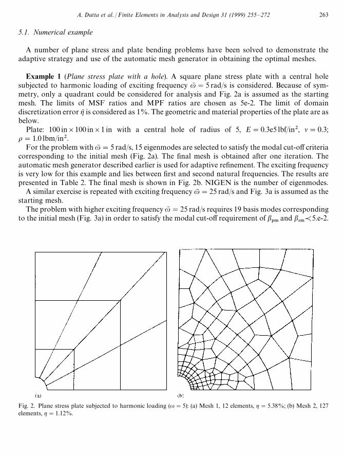
A simply supported skew plate subjected to a suddenly applied pressure load is also considered.Material properties are the same as mentioned above. The overall domain discretization errortolerance gN is kept as 9% and b

1.p1.e-3. The analysis is carried out for the full plate of size

300]300]3 in 3. The initial mesh has nine elements and the mesh is shown in Fig. 7a. Thisproblem is considered since it is expected that stress concentrations will occur near the cornerswhere the edges meet at an obtuse angle and hence such a problem is very interesting from thepoint of view of adaptive analysis.

The optimal mesh (Fig. 7c) for the simply supported skew plate subjected to a suddenly appliedpressure load is obtained following the same strategy adopted above and the results are shown inTable 6. For proper representation of the boundary conditions along the skew edges, the followingconsiderations are made.

Simply supported boundary conditions along an edge are maintained by allowing only therotation about that edge and restraining all other degrees of freedom. At a node ‘i’ (Fig. 8) along theskew edge, the rotations about normal to that skew edge can be written as

b1cos h!b

2sin h.

Using the penalty approach, this amounts to adding a term to the potential energy which can bewritten as

12C(b

1cos h!b

2sin h)2,

where C is a large number.


Fig. 5. Symmetric quadrant of clamped square plate (a/t"100) with suddenly applied point load at the centre of theplate: (a) Mesh 1, 9 elements, g"32.37%; (b) Mesh 2, 167 elements, g"5.01%; (c) Mesh 3, 313 elements, g"3.21%.


Table 5Optimal mesh for a clamped plate subjected to a suddenly applied point load at the centre of the plate

Mesh Limit of b1.

& b4.



Fig. 6. Effective stress (lbf/in2) vs. distance along the centroidal line: (a) At 1/8th cycle; (b) at 1/4th cycle; (c) at 3/8th cycle;(d) at 1/2th cycle.


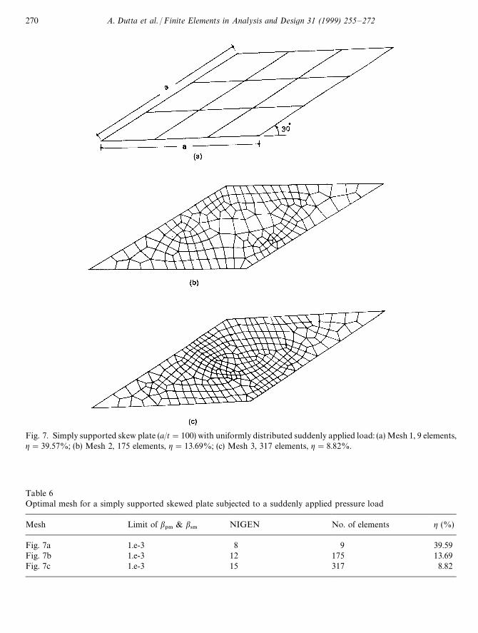
Fig. 7. Simply supported skew plate (a/t"100) with uniformly distributed suddenly applied load: (a) Mesh 1, 9 elements,g"39.57%; (b) Mesh 2, 175 elements, g"13.69%; (c) Mesh 3, 317 elements, g"8.82%.

Table 6Optimal mesh for a simply supported skewed plate subjected to a suddenly applied pressure load

Mesh Limit of b1.

& b4.




Fig. 8. Node ‘i’ along skew edge.

This can be rearranged as

12[b

1b2]C

C cos2 h !C sin h cos h

!C sin h cos h C sin2 h DGb1

b2H.

The terms C cos h2, !C sin h cos h and c sin h2 get added to the stiffness matrix, for every node onthe incline and the new stiffness matrix is solved for the unknown variables. Similar considerationsare made for translational degrees of freedom. Two iterations are required to arrive at the finalmesh. The intermediate mesh (Fig. 7b) and the final mesh (Fig. 7c) show that the refinementrequirement is more near the corners where the two adjoining edges meet at an obtuse angle.

6. Conclusion

The error estimation scheme for plane stress/plane strain and general plate and shell problemssubjected to transient dynamic loads is computationally efficient and easily implementable. Localerror indicators combined with adaptive meshing is very useful, leading to solutions of specifiedaccuracy. The overall strategy is very effective in achieving high level of accuracy introducing onlythe required additional degrees of freedom during mesh refinement.

References

[1] O.C. Zienkiewicz, Y.M. Xie, A simple error estimator and adaptive time stepping procedure for dynamic analysis,Earthquake Eng. Struct. Dyn. 20 (1991) 871—887.

[2] L.F. Zeng, N.-E. Wiberg, X.D. Li, Y.M. Xie, A posteriori local error estimation and adaptive time-stepping forNewmark Integration in dynamic analysis, Earthquake Eng. Struct. Dyn. 21 (1992) 555—571.

[3] L.F. Zeng, N.-E. Wiberg, Spatial mesh adaptation in semidiscrete finite element analysis of linear elastodynamicproblems, Comput. Mech. 9 (1992) 315—332.

[4] N.E. Wiberg, X.D. Li, A post-processed error estimate and an adaptive procedure for the semidiscrete finite elementmethod in dynamic analysis, Int. J. Numer. Meth. Eng. 37 (1994) 3585—3603.

[5] K.J. Joo, E.L. Wilson, An adaptive finite element technique for structural dynamic analysis, Comput. Struct. 30 (6)(1988) 1319—1339.


[6] R.D. Cook, J. Avrashi, Error estimation and adaptive meshing for vibration problems, Comput. Struct. 44 (3) (1992)619—626.

[7] A. Dutta, C.V. Ramakrishnan, Error estimation in finite element transient dynamic analysis using modal superposi-tion method, Eng. Comput. 14 (1) 1997.

[8] O.C. Zienkiewicz, J.Z. Zhu, A simple error estimator and adaptive procedure for practical engineering analysis, Int.J. Numer. Meth. Eng. 24 (1987) 337—357.

[9] A. Sinha, C.V. Ramakrishnan, Growth methods and binary space partitioning for efficient finite element meshgeneration, Internal Report, Applied Mechanics Dept., IIT, Delhi (1998).

[10] S. Ahmad, B.M. Irons, O.C. Zienkiewicz, Analysis of thick and thin shell structures by curved finite elements, Int. J.Num. Meth. Eng. 2 (1970) 419—451.

[11] E. Hinton, J.S. Campbell, Local and global smoothing of discontinuous finite element functions using a leastsquares method, Int. J. Num. Meth. Eng. 8 (1974) 461—480.

[12] O.C. Zienkiewicz, J.Z. Zhu, The superconvergent patch recovery and a posteriori error estimates. Part 1: therecovery technique, Int. J. Num. Meth. Eng. 33 (1992) 1331—1364.

[13] J.Z. Zhu, O.C. Zienkiewicz, E. Hinton, J. Wu, A new approach to the development of automatic quadrilateral meshgeneration, Int. J. Num. Meth. Eng. 32 (1991) 849—866.

[14] C.K. Lee, S.H. Lo, A new scheme for the generation of a graded quadrilateral mesh, Comput. Struct. 52 (5) (1994)847—857.

[15] R.J. Cass, S.E. Benzley, R.J. Meyers, T.D. Blacker, Generalized 3-D paving: An automated quadrilateral surfacemesh generation algorithm, Int. J. Num. Meth. Eng. 39 (1996) 1475—1489.

[16] S.H. Lo, Automatic mesh generation and adaptation by using contours, Int. J. Num. Meth. Eng. 31 (1991) 689—707.[17] J. Peraire, M. Vahdati, K. Morgan, O.C. Zienkiewicz, Adaptive remeshing for compressible flow computations,

J. Comp. Phys. 72 (2) (1987) 449—466.


Adaptive finite element analysis of structures under transient dynamic loading using modal...

Documents

Transcript of Adaptive finite element analysis of structures under transient dynamic loading using modal...