Investigations into the complexity of some propositional calculi
129
INVESTIGATIONS INTO THE COMPLEXITY OF SOME PROPOSITIONAL CALCULI by Marcello D’Agostino Oxford University Computing Laboratory Programming Research Group
Transcript of Investigations into the complexity of some propositional calculi

INVESTIGATIONS INTO THE COMPLEXITY
OF SOME PROPOSITIONAL CALCULI
by
Marcello D’Agostino
Oxford University Computing Laboratory
Programming Research Group

INVESTIGATIONS INTO THE COMPLEXITY
OF SOME PROPOSITIONAL CALCULI
by
Marcello D’Agostino
Technical Monograph PRG-88ISBN 0-902928-67-8
November 1990
Oxford University Computing LaboratoryProgramming Research Group11 Keble RoadOxford OX1 3QDEngland

Copyright c© 1995 Marcello D’Agostino
Oxford University Computing LaboratoryProgramming Research Group11 Keble RoadOxford OX1 3QDEngland
Electronic mail: [email protected] (JANET)

ERRATA
“Investigations into the complexityof some propositional calculi”
by
Marcello D’Agostino
• Page 6, line 21
“in their philophical” should read as “in their philosophical”
• Page 20, line 19
extra right parenthesis
• Page 30, line 15
“. . . to the end or φ . . .” should read as “. . .to the end of φ . . .”.
• Page 31, end of line 14
“. . . in such as” should read as “. . . in such a”
• Page 32, lines 4–5
“Notice that the if part of the condition is trivial, but the only-if part is not sotrivial”should read as“Notice that the only-if part of the condition is trivial, but the if part is not sotrivial”
• Page 39, Table 3.1
The Negation rule should have A as conclusion.
• Page 44
The second rule should have A as conclusion.
• Pages 56–57
The sentence across the two pages should read as: “A proof of A from Γ is a KEND-tree with origin F and such that its undischarged assumptions are in Γ,¬A”.
• Page 62, Definition 4.2.1
“. . . for all x ∈ L.” should read as “. . . for all x ∈ Σ∗
1.”
• Page 63, first line
“. . . h(x) ≤ p(|x|)” should read as “. . . |h(x)| ≤ p(|x|)
• Page 63, lines 3–6 should read as:
“The simulation function h is then a mapping [. . .] The p-simulation relation isobviously a quasi-ordering and its symmetric closure is an equivalence relation.”
• Page 63, first two lines of section 4.3 should read as:
“In this section we shall use the notation S′ ≤p S, where S and S′ are propositionalproof systems, for ‘S p-simulates S′’ ”.
• Pag. 68, line 24
after “c ≥ 2,” add “where k is the number of variables in the input formula”.
• Page 78, line 14
“. . . there are 2m−1 distinct atomic letters” should read as “. . . there are 2m − 1distinct atomic letters”.

• Pag. 120, line 12
“this kind of analysis and that the”
should read as
“this kind of analysis and that of the”
• Bibliography, entry [Gir87b]
“Lineal logic” should read as “Linear logic”
• Bibliography, entry [Gor90]
“and belnap’s” should read as “and Belnap’s”
• Bibliography, entry [Sco73]
“Completness” should read as “Completeness”
• Bibliography, entry [Smu68c]
“gentzen systems” should read as “Gentzen systems”
• Bibliography, entry [Urq90a]
replace the address “Berkeley” with “Berlin”

WARNING
The page numbers of this electronic version do NOT correspond exactly to the pagenumbers of the printed version. Please refer to sections or subsections.

Abstract
Cut-free Gentzen systems and their semantic-oriented variant, the tableau method, con-stitute an established paradigm in proof-theory and are of considerable interest for auto-mated deduction and its applications. In this latter context, their main advantage overresolution-based methods is that they do not require reduction in clausal form; on theother hand, resolution is generally recognized to be considerably more efficient within thedomain of formulae in clausal form.
In this thesis we analyse and develop a recently-proposed alternative to the tableaumethod, the system KE [Mon88a,Mon88b]. We show that KE, though being ‘close’ tothe tableau method and sharing all its desirable features, is essentially more efficient.We trace this phenomenon to the fact that KE establishes a closer connection with theintended (classical, bivalent) semantics. In particular we point out, in Chapter 2, a basic‘redundancy’ in tableau refutations (or cut-free Gentzen proofs) which depends on theform of the propositional inference rules and, therefore, affects any procedure based onthem. In Chapter 3 we present the system KE and show that it is not affected by thiskind of redundancy. An important property of KE is the analytic cut property : cutscannot be eliminated but can be restricted to subformulae of the theorem, so that thesubformula principle is still obeyed. We point out the close relationship between KE andthe resolution method within the domain of formulae in clausal form. In Chapter 4 weundertake an analysis of the complexity of the propositional fragment of KE relative tothe propositional fragments of other proof systems, including the tableau method andnatural deduction, and prove some simulation and separation results. We show, amongother things, that KE and the tableau method are separated with respect to the p-simulation relationship (KE can linearly simulate the tableau method, but the tableaumethod cannot p-simulate KE). In Chapter 5 we consider Belnap’s four-valued logic,which has been proposed as an alternative to classical logic for reasoning in the presenceof inconsistencies, and develop a tableau-based as well as a KE-based refutation system.Finally, in Chapter 6, we generalize on the ideas contained in the previous chapters andprove some more simulation and separation results.
Acknowledgements
This monograph consists of my thesis submitted for the degree of Doctor ofPhilosophy in the University of Oxford. I wish to thank my supervisors, JoeStoy and Roberto Garigliano, for their encouragement, advice and guidanceduring the course of this thesis. Thanks are also due to Marco Mondadorifor his invaluable comments and suggestions. I have also benefitted fromconversations with Ian Gent, Rajev Gore, Angus Macintyre, Paolo Mancosu,Bill McColl, Claudio Pizzi, Alasdair Urquhart, Lincoln Wallen and AlexWilkie.
I also wish to thank Dov Gabbay for providing me with a draft of aforthcoming book of his; Peter Aczel and Alan Bundy for giving me theopportunity to discuss my work in seminars given at Manchester and Edin-burgh, and Michael Mainwaring for doing his best to make my English moreacceptable.
I am grateful to my parents and to all my friends, especially to GabriellaD’Agostino for her usual impassioned support.
This research has been supported by generous grants awarded by theItalian Ministry of Education, the City Council of Palermo (‘Borsa di studioNinni Cassara’) and CNR-NATO.

Contents
1 Introduction 5
2 The redundancy of cut-free proofs 122.1 Invertible sequent calculi . . . . . . . . . . . . . . . . . . . . . 122.2 From sequent proofs to tableau refutations . . . . . . . . . . . 152.3 Cut-free proofs and bivalence . . . . . . . . . . . . . . . . . . 162.4 The redundancy of cut-free proofs . . . . . . . . . . . . . . . 192.5 The culprit . . . . . . . . . . . . . . . . . . . . . . . . . . . . 212.6 Searching for a countermodel . . . . . . . . . . . . . . . . . . 23
2.6.1 Expansion systems . . . . . . . . . . . . . . . . . . . . 262.6.2 Redundant trees . . . . . . . . . . . . . . . . . . . . . 29
3 An alternative approach 313.1 Bivalence restored . . . . . . . . . . . . . . . . . . . . . . . . 313.2 The system KE . . . . . . . . . . . . . . . . . . . . . . . . . . 323.3 Soundness and completeness of KE . . . . . . . . . . . . . . . 36
3.3.1 Completeness of KE: proof one . . . . . . . . . . . . . 383.3.2 Completeness of KE: proof two . . . . . . . . . . . . . 403.3.3 The subformula principle . . . . . . . . . . . . . . . . 42
3.4 KE and the Davis-Putnam Procedure . . . . . . . . . . . . . 443.5 The first-order system KEQ . . . . . . . . . . . . . . . . . . 463.6 Soundness and completeness of KEQ . . . . . . . . . . . . . 473.7 A digression on direct proofs: the system KI . . . . . . . . . 493.8 Analytic natural deduction . . . . . . . . . . . . . . . . . . . 513.9 Non-classical logics . . . . . . . . . . . . . . . . . . . . . . . . 53
4 Computational complexity 544.1 Absolute and relative complexity . . . . . . . . . . . . . . . . 544.2 Relative complexity and simulations . . . . . . . . . . . . . . 574.3 An overview . . . . . . . . . . . . . . . . . . . . . . . . . . . . 584.4 Are tableaux an improvement on truth-tables? . . . . . . . . 61
1

2 CONTENTS
4.5 The relative complexity of KE and KI . . . . . . . . . . . . . 654.5.1 KE versus KI . . . . . . . . . . . . . . . . . . . . . . 664.5.2 KE versus the tableau method . . . . . . . . . . . . . 674.5.3 KE versus Natural Deduction . . . . . . . . . . . . . . 744.5.4 KE and resolution . . . . . . . . . . . . . . . . . . . . 77
4.6 A more general view . . . . . . . . . . . . . . . . . . . . . . . 77
5 Belnap’s four valued logic 835.1 Introduction . . . . . . . . . . . . . . . . . . . . . . . . . . . . 835.2 ‘How a computer should think’ . . . . . . . . . . . . . . . . . 845.3 Belnap’s four-valued model . . . . . . . . . . . . . . . . . . . 845.4 Semantic tableaux for Belnap’s logic . . . . . . . . . . . . . . 87
5.4.1 Propositional tableaux . . . . . . . . . . . . . . . . . . 875.4.2 Detecting inconsistencies . . . . . . . . . . . . . . . . 925.4.3 First-order tableaux . . . . . . . . . . . . . . . . . . . 94
5.5 An efficient alternative . . . . . . . . . . . . . . . . . . . . . . 97
6 A generalization: cut systems 1036.1 Proper derived rules . . . . . . . . . . . . . . . . . . . . . . . 1036.2 Cut systems . . . . . . . . . . . . . . . . . . . . . . . . . . . . 1076.3 Analytic cut systems versus cut-free systems . . . . . . . . . . 109
7 Conclusions 111

List of Figures
2.1 A closed tableau for {A ∨ B,A ∨ ¬B,¬A ∨ C,¬A ∨ ¬C} . . 222.2 A typical pattern. . . . . . . . . . . . . . . . . . . . . . . . . . 232.3 Redundancy of tableau refutations. . . . . . . . . . . . . . . . 24
3.1 Two different analyses. . . . . . . . . . . . . . . . . . . . . . . 333.2 A KE-refutation of {A ∨ B,A ∨ ¬B,¬A ∨ C,¬A ∨ ¬C} . . . 38
4.1 A KE-refutation of HP1,P2,P3. . . . . . . . . . . . . . . . . . 69
4.2 A KE-refutation of H3. . . . . . . . . . . . . . . . . . . . . . 73
5.1 A proof of ((A ∨ B) ∧ ¬A) → (B ∨ (A ∧ ¬A)) . . . . . . . . . 905.2 A failed attempt to prove the disjunctive syllogism . . . . . . 915.3 An REfde-proof of ((A ∨ B) ∧ ¬A) → (B ∨ (A ∧ ¬A)) . . . . 98
3
List of Tables
2.1 Sequent rules for classical propositional logic. . . . . . . . . . 142.2 Propositional tableau rules for unsigned formulae. . . . . . . 17
3.1 KE rules for unsigned formulae. . . . . . . . . . . . . . . . . 373.2 CNF reduction rules. . . . . . . . . . . . . . . . . . . . . . . . 443.3 Generalized KE rules. . . . . . . . . . . . . . . . . . . . . . . 45
4.1 A sequent-conclusion natural deduction system. . . . . . . . 76
5.1 Propositional tableau rules for Belnap’s four valued logic. . . 885.2 Formulae of type α. . . . . . . . . . . . . . . . . . . . . . . . 885.3 Formulae of type β. . . . . . . . . . . . . . . . . . . . . . . . 895.4 The rules of REfde. . . . . . . . . . . . . . . . . . . . . . . . . 97
4

Chapter 1
Introduction
Traditionally, proof theory has been concerned with formal representationsof the notion of proof as it occurs in mathematics or other intellectual activ-ities, regardless of the efficiency of such representations. The rapid develop-ment of computer science has brought about a dramatic change of attitude.Efficiency has become a primary concern and this fact has given rise to awhole new area of research in which the ‘old’ questions about provability,completeness, decidability, etc. have been replaced by new ones, with consid-erations of complexity playing a major role. A formal representation whichis complete in principle may turn out to be ‘practically incomplete’ becausein some cases it requires unrealistic resources (in terms of computer timeand memory). As a result of this change of perspective, formal represen-tations which are equivalent with respect to the consequence relation thatthey represent, can be seen to be essentially separated as to their practicalscope.
Nowhere has this shift of emphasis been more apparent than in the fieldof propositional logic. Here the neglected star is back in the limelight. Openquestions of theoretical computer science like P =?NP and NP =?co-NPhave revitalized a subject which seemed to be ‘saturated’ and to deserveonly a brief mention as a stepping stone to the ‘real thing’. But the interestin propositional logic is not restricted to these fundamental open questions.There is a plethora of problems which are perhaps less fundamental but ofpractical and theoretical importance. Many of them arise when we considerlogic as a tool. This was certainly the attitude of the pioneers of formallogic, from Aristotle to Leibniz. The latter dreamt of a calculus ratiocinatorof which mathematical logic would be the heart, and explicitly related theimportance of his project to its potential ‘usefulness’:
For if praise is given to the men who have determined the number
5

6 CHAPTER 1. INTRODUCTION
of regular solids — which is of no use, except insofar as it ispleasant to contemplate — and if it is thought to be an exerciseworthy of a mathematical genius to have brought to light themore elegant property of a conchoid or cissoid, or some otherfigure which rarely has any use, how much better will it be tobring under mathematical laws human reasoning, which is themost excellent and useful thing we have1.
Later the role of logic in the foundations of mathematics took over and,while this opened up an entire world of conceptual and technical subtleties,it also brought about the neglect of many interesting questions2. Amongsuch questions are all those related to the direct use of logic to solve prob-lems about our ‘world’ (or our database), that is as a partial realizationof Leibniz’s dream. In the second half of this century, the revival of Leib-niz’s program (known as ‘automated deduction’) as well as the significantrole played by a variety of logical methods in both theoretical and appliedcomputer science, has resulted in a greater awareness of the computationalaspects of logical systems and a closer (or at least a fresh) attention to theirproof-theoretical representations. As Gabbay has stressed [Gab91, Gab90]logical systems ‘which may be conceptually far apart (in their philosophi-cal motivation and mathematical definitions), when it comes to automatedtechniques and proof-theoretical presentation turn out to be brother andsister’[Gab91, Section 1.1]. On the other hand, the same logical system(intended as a set-theoretical definition of a consequence relation) usuallyadmits of a wide variety of proof-theoretical representations which may re-veal or hide its similarities with other logical systems3. The considerationof these phenomena has prompted Gabbay to put forward the view that
[. . . ] a logical system L is not just the traditional consequence re-lation ⊢, but a pair (⊢,S⊢), where ⊢ is a mathematically defined
1[Par66, page 166].2In his survey paper [Urq92a] Alasdair Urquhart mentions the simplification of Boolean
formulae. ‘Here the general problem takes the form: how many logical gates do we need torepresent a given Boolean function? This is surely as simple and central a logical problemthat one could hope to find; yet, in spite of Quine’s early contributions, the whole areahas been simply abandoned by most logicians, and is apparently thought to be fit only forengineers.’ He also remarks that ‘our lack of understanding of the simplification problemretards our progress in the area of the complexity of proofs.’
3As an example of this approach, Gabbay observes that ‘it is very easy to move fromthe truth-table presentation of classical logic to a truth-table system for Lukasiewicz’sn-valued logic. It is not so easy to move to an algorithmic system for intuitionistic logic.In comparison, for a Gentzen system presentation, exactly the opposite is true. Intu-itionistic and classical logic are neighbours, while Lukasiewicz’s logics seem completeleydifferent.’[Gab91, Section 1.1].

7
consequence relation (i.e. a set of pairs (∆, Q) such that ∆ ⊢ Q)and S⊢ is an algorithmic system for generating all those pairs.Thus, according to this definition, classical logic ⊢ perceived asa set of tautologies together with a Gentzen system S⊢ is notthe same as classical logic together with the two-valued truth-table decision procedure T⊢ for it. In our conceptual framework,(⊢,S⊢) is not the same logic as (⊢,T⊢)4.
Gabbay’s proposal seems even more suggestive when considerations of com-putational complexity enter the picture. Different proof-theoretical algo-rithms for generating the same consequence relation may have different com-plexities. Even more interesting: algorithmic representations which appear‘close’ to each other from the proof-theoretical point of view may show dra-matic differences as far as their efficiency is concerned. A significant part ofthis work will be devoted to illustrate this somewhat surprising phenomenon.
In the tradition which considers formal logic as an organon of thought5 acentral role has been played by the ‘method of analysis’, which amounts towhat today, in the computer science circles, is called a ‘bottom-up’ or ‘goal-oriented’ procedure. Though the method was largely used in the mathemat-ical practice of the ancient Greeks, its fullest description can be found inPappus (3rd century A.D.), who writes:
Now analysis is a method of taking that which is sought asthough it were admitted and passing from it through its con-sequences in order, to something which is admitted as a resultof synthesis; for in analysis we suppose that which is sought bealready done, and we inquire what it is from which this comesabout, and again what is the antecedent cause of the latter, andso on until, by retracing our steps, we light upon something al-
4[Gab91, Section 1.1].5Of course, as a matter of historical fact, logicians do not need to be full-time repre-
sentatives of a single tradition. Leibniz is perhaps the best example: while he emphasizedthe practical utility of his dreamt-of calculus of reason to solve verbal disputes, he alsoclaimed that the whole of mathematics could be reduced to logical principles, indeed tothe sole principle of identity; this made him a precursor of the logicist tradition in the phi-losophy of mathematics. Gentzen, who certainly belonged to the ‘foundational’ tradition,showed some concern for the practical aspects of his own work. Among the advantagesof his calculus of natural deduction he mentioned that ‘in most cases the derivations fortrue formulae are shorter [. . . ] than their counterparts in logistic calculi’[Gen35, page 80].A brilliant representative of both traditions is Beth: he was involved in the practical aswell as the foundational aspects of logic. His emphasis on the advantages of the tableaumethod as a tool for drawing inferences is pervasive and, as we will see, even excessive.
8 CHAPTER 1. INTRODUCTION
ready known or ranking as a first principle; and such a methodwe call analysis, as being a solution backwards6.
This is the so-called directional sense of analysis. The idea of an ‘analyticmethod’, however, is often associated with another sense of ‘analysis’ whichis related to the ‘purity’ of the concepts employed to obtain a result and,in the framework of proof-theory, to the subformula principle of proofs.In Gentzen’s words: ‘No concepts enter into the proof other than thosecontained in its final result, and their use was therefore essential to theachievement of that result’[Gen35, p. 69] so that ‘the final result is, as itwere, gradually built up from its constituent elements [Gen35, p.88]. Bothmeanings of analysis have been represented, in the last fifty years, by thenotion of a cut-free proof in Gentzen’s sense: not only cut-free proofs employno concepts outside those contained in the statement of the theorem, butthey can also be discovered by means of simple ‘backwards’ procedures likethat described by Pappus. Therefore Gentzen-style cut-free methods (whichinclude their semantic-flavoured descendant, known as ‘the tableau method’)were among the first used in automated deduction7 and are today enjoyinga deserved revival8 which is threatening the unchallenged supremacy thatresolution and its refinements9 have had for over two decades in the area ofautomated deduction and logic programming.
There are indeed several reasons which may lead us to prefer cut-freeGentzen methods to resolution as a basis for automated deduction as wellas for other applications, like program verification. First, unlike resolution,these methods do not require reduction in any normal form, which fact allowsthem to exploit the full power of first order logic10. Second, the derivationsobtained constitute an acceptable compromise between ‘machine-oriented’tests for validity, like resolution derivations, and ‘human-oriented’proofs, likethose constructed in the framework of natural deduction calculi; this makesthem more suitable for ‘interactive’ use. Third, they admit of natural exten-sions to a wide variety of non-classical logics11 which appear less contrived
6[Tho41] pp. 596–599.7See, for example, [Bet58], [Wan60], [Kan63]. Cfr. also [Dav83] and [MMO83].8[Fit90] and [Gal86] are recent textbooks on ‘logic for computer science’ which are en-
tirely based on the tableau method and on cut-free Gentzen systems respectively. [Wal90]is a book which combines the technical power of Bibel’s connection method [Bib82] withthe conceptual clarity of the tableau representation of classical as well as non-classicallogic. [OS88] is a recent example of a complete theorem-prover based on the tableaumethod.
9See [CL73] and [Sti86] for an overview.10On this point see [Cel87].11For Intuitionistic and Modal logics, see [Fit83]; see also [Wal90] for a tableau-oriented
extension of Bibel’s connection method to intuitionistic and modal logics; for relevance

9
than their resolution-based counterparts12.On the other hand, there is one reason, which usually leads us to prefer
some form of resolution: efficiency. As will be shown in Chapter 4 cut-free methods are hopelessly inefficient and lead to combinatorial explosionin fairly simple examples which are easily solved not only by resolutionbut even by the old, despised truth-tables. What is the ultimate cause ofthis inefficiency? Can it be remedied? The main contribution of our workis a clarification of this issue and a positive proposal motivated thereby.The clarification can be expressed as a paradox: the ultimate cause of theinefficiency of cut-free methods is exactly what has traditionally made themso useful both from the theoretical and practical point of view, namely theirbeing cut-free. But, as Smullyan once remarked, ‘The real importance ofcut-free proofs is not the elimination of cuts per se, but rather that suchproofs obey the subformula principle.’13 Apart from Smullyan’s short papercited above, however, the proof-theory of analytic cut systems, i.e. systemswhich allow cuts but limit their application so that the resulting proofs stillobey the subformula principle, has not been adequately studied, and thesame is true of their relative complexity14. In this work we shall take somesteps in a forward direction. Moreover, while considerations of efficiency areusually strictly technical and unconnected with more conceptual issues, forexample semantical issues, we shall make a special and, we hope, successfuleffort to bring out a clear connection between computational efficiency onthe one hand, and a close correspondence with the underlying (classical)semantics on the other.
We shall base our study on a particular system, the system KE, recentlyproposed by Mondadori [Mon88a, Mon88b] as an alternative to the tableaumethod for classical logic. As will be argued, KE is in some sense idealfor our purposes in that it constitutes a refutation system which, thoughbeing proof-theoretically ‘close’ to the tableau method, is essentially moreefficient. Moreover, it is especially suited to the purpose of illustrating theconnection between efficiency, analytic cut and classical semantics, which isthe object of our study.
In Chapter 2, we examine what we call the ‘redundancy of cut-free proofs’as a phenomenon which depends on the form of the cut-free rules themselves
logics see [TMM88]; for many-valued logics see [Car87]; for linear logic see [Gir87b] and[Avr88].
12See [FE89] and [Fit87]. For a review of these and other resolution-based methods fornon-classical logics, see [Wal90].
13[Smu68b], p. 560.14For a recent exception see [Urq92b].

10 CHAPTER 1. INTRODUCTION
and not on the way in which they are applied : this phenomenon affects cut-free systems intended as non-deterministic algorithms for generating proofsand therefore affects every proof generated by them. We relate this intrinsicredundancy to the fact that the cut-free rules do not reflect, in some sense,the (classical bivalent) structure of their intended semantics. In Chapter 3we develop an alternative approach based on Mondadori’s system KE whichis not cut-free yet obeys the subformula principle (and also a stronger nor-mal form principle), so preserving the most important property of cut-freesystems. The system KE is a refutation system which, like the tableaumethod, generates trees of (signed or unsigned) formulae by means of treeexpansion rules. Its distinguishing feature is that its only branching ruleis the rule PB (Principle of Bivalence) which is closely related to the cutrule of Gentzen systems. So, in spite of all the similarities, KE hinges upona rule whose absence is typical of the tableau method (and of all cut-freesystems). An important related property of KE is the analytic cut property :cuts are not eliminable but can be restricted to analytic ones, involving onlysubformulae of the theorem. We also show that the set of formulae to beconsidered as cut formulae can be further restricted as a result of a strongnormal form theorem.
In Chapter 4, after briefly reviewing the most important results on therelative complexity of propositional calculi, we examine how the use of ana-lytic cuts affects the complexity of proofs. We show that KE (and, in fact,any analytic cut system) is essentially more efficient than the tableau method(or any cut-free system). These results should be read in parallel with thesemantic-oriented analysis carried out in Chapter 2: KE establishes a closeconnection with classical (bivalent) semantics which the tableau method failsto do, and this very fact has important consequences from the computationalpoint of view.
Like the tableau method, KE can be adapted to a variety of non-classicallogics including intuitionistic and modal logics. All these non-classical ver-sions can be obtained trivially, given the corresponding tableau-based sys-tems, as explained in Section 3.9. In Chapter 5 we shall examine a newcase: Belnap’s four-valued logic. This is a form of relevant logic which hasalso an interesting motivation from the point of view of computer science,since it is intended to formalize the notion of deduction from inconsistentdatabases. We formulate a tableau-based and a KE-based system both ofwhich, as in the case of classical two-valued logic, generate simple binarytrees. These systems are based on a reformulation of Belnap’s four-valuedsemantics which ‘mimics’ the bivalent structure of classical semantics and,to the best of our knowledge, is new to the literature. Although Belnap’slogic is a restriction of classical logic (intended as a consequence relation),

11
our systems can be seen as extensions of the corresponding classical systemsin that they allow us to characterize simultaneously the classical two-valuedand Belnap’s four-valued consequence relations using the same formal ma-chinery.
Finally, in Chapter 6, we generalize on the ideas contained in the previouschapters. We show that, as far as the complexity of ‘conventional’ (analyticand non-analytic) proof systems is concerned, the cut rule is all that mattersand the form of the logical rules (under certain conditions) does not play anysignificant role. This chapter finalizes the process started in Chapter 2: whatin Gentzen-type systems is eliminable (and indeed its eliminability providesa major motivation for the form of the rules) becomes, in ‘cut systems’, theonly essential feature.

Chapter 2
The redundancy of cut-free
proofs
2.1 Invertible sequent calculi
Gentzen introduced the sequent calculi LK and LJ as well as the natural de-duction calculi NK and NJ in his famous 1935 paper [Gen35]. Apparentlyhe considered the sequent calculi as technically more convenient for meta-logical investigation1. In particular he thought that they were ‘especiallysuited to the purpose’ of proving the Hauptsatz and that their form was‘largely determined by considerations connected with [this purpose]’2. Hecalled these calculi ‘logistic’ because, unlike the natural deduction calculi,they do not involve the introduction and subsequent discharge of assump-tions, but deal with formulae which are ‘true in themselves, i.e. whose truthis no longer conditional on the truth of certain assumption formulae’3. Such‘unconditional’ formulae are sequents, i.e. expressions of the form
A1, . . . , An ⊢ B1, . . . , Bn(2.1)
(where the Ai’s and the Bi’s are formulae) with the same informal meaningas the formula
A1 ∧ . . . ∧ An → B1 ∨ . . . ∨ Bm.
The sequence to the left of the turnstyle is called ‘the antecedent’ and thesequence to the right is called ‘the succedent’. In the case of intuitionisticlogic the succedent may contain at most one formula. In this chapter weshall consider the classical system and focus on the propositional rules.
1[Gen35], p. 69.2[Gen35, p. 89].3[Gen35], p. 82.
12

2.1. INVERTIBLE SEQUENT CALCULI 13
Although Gentzen considered the antecedent and the succedent as se-quences, it is often more convenient to use sets, which eliminates the needfor ‘structural’ rules to deal with permutations and repetitions of formulae4.Table 2.1 shows the rules of Gentzen’s LK once sequences have been re-placed by sets (we use Γ,∆, etc. for sets of formulae and write Γ, A as anabbreviation of Γ ∪ {A}). A proof of a sequent Γ ⊢ ∆ consists of a tree ofsequents built up in accordance with the rules and on which all the leavesare axioms. Gentzen’s celebrated Hauptsatz says that the cut rule can beeliminated from proofs. This obviously implies that the cut-free fragment iscomplete. Furthermore, one can discard the last structural rule left — thethinning rule — and do without structural rules altogether without affect-ing completeness, provided that the axioms are allowed to have the moregeneral form
Γ, A ⊢ ∆, A.
This well-known variant corresponds to Kleene’s system G4 [Kle67, chapterVI].
Gentzen’s rules have become a paradigm both in proof-theory and in itsapplications. This is not without reason. First, like the natural deductioncalculi, they provide a precise analysis of the logical operators by specifyinghow each operator can be introduced in the antecedent or in the succedent ofa sequent5. Second, their form ensures the validity of the Hauptsatz : eachproof can be transformed into one which is cut-free, and cut-free proofsenjoy the subformula property : every sequent in the proof tree contains onlysubformulae of the formulae in the sequent to be proved.
From a conceptual viewpoint this property represents the notion of apurely analytic or ‘direct’ argument6: ‘no concepts enter into the proof other
4This reformulation is adequate for classical and intuitionistic logic, but not if one wantsto use sequents for some other logic, like relevance or linear logic, in which the numberof occurrences of formulae counts. For such logics the antecedent and the succedent areusually represented as multisets; see [TMM88] and [Avr88].
5Whereas in the natural deduction calculi there are, for each operator, an introductionand an elimination rule, in the sequent calculi there are only introduction rules and theeliminations take the form of introductions in the antecedent. Gentzen seemed to considerthe difference between the two formulations as a purely technical aspect. See [Sun83]. Healso suggested that the rules of the natural deduction calculus could be seen as definitions
of the operators themselves. In fact he argued that the introduction rules alone aresufficient for this purpose and that the elimination rules are ‘no more, in the final analysis,than consequences of these definitions’[Gen35, p. 80]. He also observed that this ‘harmony’is exhibited by the intuitionistic calculus but breaks down in the classical case. For athorough discussion of this subtle meaning-theoretical issue the reader is referred to thewritings of Michael Dummett and Dag Prawitz, in particular [Dum78] and [Pra78].
6On this point see [Sta77].

14 CHAPTER 2. THE REDUNDANCY OF CUT-FREE PROOFS
Axioms
A ⊢ A
Structural rules
Γ ⊢ ∆[Thinning]
Γ,Θ ⊢ ∆,Λ
Γ, A ⊢ ∆ Γ ⊢ ∆, A[Cut]
Γ ⊢ ∆
Operational rules
Γ, A ⊢ ∆ Γ, B ⊢ ∆[I-∨left]
Γ, A ∨ B ⊢ ∆
Γ ⊢ ∆, A Γ ⊢ ∆, B[I-∧right]
Γ ⊢ ∆, A ∧ B
Γ, A,B ⊢ ∆[I-∧left]
Γ, A ∧ B ⊢ ∆
Γ ⊢ ∆, A,B[I-∨right]
Γ ⊢ ∆, A ∨ B
Γ ⊢ ∆, A Γ, B ⊢ ∆[I-→left]
Γ, A → B ⊢ ∆
Γ, A ⊢ ∆, B[I-→right]
Γ ⊢ ∆, A → B
Γ ⊢ ∆, A[I-¬left]
Γ,¬A ⊢ ∆
Γ, A ⊢ ∆[I-¬right]
Γ ⊢ ∆,¬A
Table 2.1: Sequent rules for classical propositional logic.
2.2. FROM SEQUENT PROOFS TO TABLEAU REFUTATIONS 15
than those contained in its final result, and their use was therefore essentialto the achievement of that result’[Gen35, p. 69]. Third, the rules of a cut-freesystem, like Kleene’s G4, seem to be particularly suited to a ‘goal-oriented’search for proofs: instead of going from the axioms to the endsequent, onecan start from the endsequent and use the rules in the reverse direction,going from the conclusion to suitable premises from which it can be derived.This method, which is clearly reminiscent of Pappus’ ‘theoretical analysis’7,works only in virtue of an important property of the rules of G4 describedin Lemma 6 of [Kle67], namely their invertibility.
Definition 2.1.1 A rule is invertible if the provability of the sequent belowthe line in each application of the rule implies the provability of all thesequents above the line.
As was early recognized by the pioneers of Automated Deduction8, if a log-ical calculus has to be employed for this kind of ‘bottom-up’ proof-searchit is essential that its rules be invertible: this allows us to stop as soon aswe reach a sequent that we can recognize as unprovable (for instance onecontaining only atomic formulae and in which the antecedent and the succe-dent are disjoint) and conclude that the initial sequent is also unprovable.We should notice that the absence of the thinning rule is crucial in thiscontext because it is easy to see that the thinning rule is not invertible: theprovability of its conclusion does not imply, in general, the provability of thepremise.
2.2 From sequent proofs to tableau refutations
As far as classical logic is concerned, a system like G4 admits of an inter-esting semantic interpretation.
Let us say that a sequent Γ ⊢ ∆ is valid if every situation (i.e. a booleanvaluation) which makes all the formulae in Γ true, also makes true at leastone formula in ∆. Otherwise if some situation makes all the formulae in Γtrue and all the formulae in ∆ false, we say that the sequent is falsifiableand that the situation provides a countermodel to the sequent.
According to this semantic viewpoint we prove that a sequent is validby ruling out all possible falsifying situations. So a sequent Γ ⊢ ∆ repre-sents a valuation problem: find a boolean valuation which falsifies it. Thesoundness of the rules ensures that a valuation which falsifies the conclusionmust also falsify at least one of the premises. Thus, if applying the rules
7See the Introduction above.8See for instance [Mat62].

16 CHAPTER 2. THE REDUNDANCY OF CUT-FREE PROOFS
backwards we reach an axiom in every branch, we are allowed to concludethat no falsifying valuation is possible (since no valuation can falsify an ax-iom) and that the endsequent is therefore valid. On the other hand, theinvertibility of the rules allows us to stop as soon as we reach a falsifiablesequent and claim that any falsifying valuation provides a countermodel tothe endsequent. Again, if the thinning rule were allowed, we would not bebe able, in general, to retransmit falsifiability back to the endsequent. So, ifemployed in bottom-up search procedures, the thinning rule may result inthe loss of crucial semantic information.
Beth, Hintikka, Schutte and Kanger (and maybe more) independently showed,in the ‘50s, how this semantic interpretation provided a strikingly simple andinformative proof of Godel’s completeness theorem9. Their results suggestedthat the semantic interpretation could be presented as a proof method onits own, in which sequents do not appear and complex formulae are progres-sively ‘analysed’ into their successive components. This approach was laterdeveloped and perfected by Smullyan with his method of ‘analytic tableaux’[Smu68a].
The construction of an analytic tableau for a sequent Γ ⊢ ∆ closelycorresponds to the systematic search for a countermodel outlined aboveexcept that Smullyan’s presentation uses trees of formulae instead of treesof sequents. The correspondence between the tableau formulation and thesequent formulation is illustrated in detail in Smullyan’s book [Smu68a] towhich we refer the reader10. The propositional tableau rules (for unsignedformulae) are listed in Table 2.2.
2.3 Cut-free proofs and bivalence
This evolution from the original LK system to Smullyan’s system of ‘analytictableaux’ took over thirty years but did not change Gentzen’s formulationsignificantly. However, Gentzen’s rules are not the only possible way ofanalysing the classical operators and not necessarily the best for all purposes.The form of Gentzen’s rules was influenced by considerations which werepartly philosophical, partly technical. In the first place he wanted to setup a formal system which ‘comes as close as possible to actual reasoning’11.In this context he introduced the natural deduction calculi in which theinferences are analysed essentially in a constructive way and classical logic is
9[Bet55], [Hin55], [Sch56], [Kan57].10See also [Smu68c] and [Sun83]11[Gen35], p. 68.

2.3. CUT-FREE PROOFS AND BIVALENCE 17
A ∧ B
AB
E∧ ¬(A ∧ B)
¬A ¬BE¬∧
¬(A ∨ B)
¬A¬B
E¬∨ A ∨ B
A BE∨
¬(A → B)
A¬B
E¬ → A → B
¬A BE→
¬¬A
AE¬¬
Table 2.2: Propositional tableau rules for unsigned formulae.
obtained by adding the law of excluded middle in a purely external manner.Then he recognized that the special position occupied by this law would haveprevented him from proving the Hauptsatz in the case of classical logic. Sohe introduced the sequent calculi as a technical device in order to enunciateand prove the Hauptsatz in a convenient form12 both for intuitionistic andclassical logic. These calculi still have a strong deduction-theoretical flavourand Gentzen did not show any sign of considering the relationship betweenthe classical calculus and the semantic notion of entailment which, at thetime, was considered as highly suspicious.
The approach developed in the ‘50’s by Beth and Hintikka was mainlyintended to bridge the gap between classical semantics and the theory offormal derivability. In his 1955 paper, where he introduced the method ofsemantic tableaux, Beth thought he had reached a formal method which was‘in complete harmony with the standpoint of [classical bivalent] semantics’[Bet55, p. 317]. He also claimed that this method would allow for the ‘purelymechanical’ construction of proofs which were at the same time ‘remarkablyconcise’ and could even be ‘proved to be, in a sense, the shortest ones whichare possible’ [Bet55, p. 323]. On the other hand Hintikka, who indepen-dently and simultaneously developed what amounts to the same approach,hoped that in this way he would ‘obtain a semantical theory of quantifica-tion which satisfies the highest standard of constructiveness’ [Hin55, p. 21].Both authors explicitly stressed the correspondence between their own rules
12[Gen35], p. 69.

18 CHAPTER 2. THE REDUNDANCY OF CUT-FREE PROOFS
and those put forward by Gentzen13. So two apparently incompatible aimsseemed to be achieved in the formal framework of Gentzen-type rules.
The solution to this puzzle is that the so-called semantic interpretation ofGentzen’s rules does not establish those ‘close connections between [classical]semantics and derivability theory’ that Beth tried to point out. In fact ifone takes the cut-free rules as a formal representation of classical logic, thesituation seems odd. The rule which the Hauptsatz shows to be eliminableis the cut rule:
Γ, A ⊢ ∆ Γ ⊢ ∆, A[CUT]
Γ ⊢ ∆
If we read this rule upside-down, following the same semantic interpretationthat we adopt for the operational rules, then what the cut rule says is:
In all circumstances and for all propositions A, either A is trueor A is false.
But this is the Principle of Bivalence, namely the basic principle of classicallogic. By contrast, none of the rules of the cut-free fragment implies biva-lence (as is shown by the three-valued semantics for this fragment14). Theelimination of cuts from proofs is, so to speak, the elimination of bivalencefrom the underlying semantics15.
We have, then, a rather ambiguous situation: on the one hand we havea complete set of rules which are usually taken as a convenient analyticrepresentation of classical logic; on the other hand, these rules do not assignto the basic feature of classical semantics — the Principle of Bivalence — anyspecial role in the analysis of classical inferences16. We can ask ourselves twoquestions: is the elimination of bivalence (cut) necessary? Is it harmless?
As Smullyan once remarked: ‘The real importance of cut-free proofs isnot the elimination of cuts per se, but rather that such proofs obey thesubformula principle.’17 So, our two questions can be reformulated as fol-lows: (1) Can we think of an analysis of classical inferences which gives the
13[Bet55], p. 318 and p. 323; [Hin55], p.47.14See [Gir87a], chapter 3; see also [Sch77].15Of course, the fact that the cut-free rules, in the semantic interpretation, are sound
from the standpoint of classical semantics does not necessarely mean that they are in‘complete harmony’ with this standpoint.
16Hintikka was fully aware that in his approach he was depriving the principle of biva-lence of any role. In fact he did it intentionally in order to pursue his quasi-constructivistprogram. Cfr. [Hin55], chapter III, pp. 24–26
17[Smu68b, p.560]. A problem: is there any application of cut-elimination which requiresthe proofs to be cut-free, not just to satisfy the subformula property?

2.4. THE REDUNDANCY OF CUT-FREE PROOFS 19
Principle of Bivalence the prominent role that it should have in a formalrepresentation of classical logic? (2) Would such an analysis accomplish amore concise and efficient representation of classical proofs which preservesthe most important property of the cut-free analysis (the subformula prin-ciple)?
The two questions are independent, but it is only to be expected that apositive answer to the second will be a by-product of a good answer to thefirst.
In the rest of this chapter we shall argue that the Principle of Biva-lence (i.e. some form of cut) should indeed play a role in classical analyticdeduction18; that the reintroduction of bivalence in the analysis not onlydoes not affect the subformula principle, but also allows for much shorterproofs, because it eliminates a kind of redundancy which is inherent to thecut-free analysis. In the next section we shall discuss a typical example ofthis redundancy.
2.4 The redundancy of cut-free proofs
Gentzen said that the essential property of a cut-free proof is that ‘it isnot roundabout’ [Gen35, p.69]. By this he meant that: ‘the final resultis, as it were, gradually built up from its constituent elements. The proofrepresented by the derivation is not roundabout in that it contains onlyconcepts which recur in the final result’ [Gen35, p.88]. However there is asense in which cut-free proofs are roundabout.
Let us consider, as a simple example, a cut-free proof of the sequent:
A ∨ B,A ∨ ¬B,¬A ∨ C,¬A ∨ ¬C ⊢ ∅
expressing the fact that the antecedent is inconsistent.
A minimal proof is as follows (we write the proof upside-down according tothe interpretation of the sequent rules as reduction rules in the search fora counterexample; by Γ ⊢, we mean Γ ⊢ ∅ and consider as axioms all thesequents of the form Γ, A,¬A ⊢):
18By this we do not mean that some form of cut should be ‘thrown into’ the cut-freesystem, but that some of the rules for the logical operators should be modified to allowthe cut rule to play a role in the analysis.

20 CHAPTER 2. THE REDUNDANCY OF CUT-FREE PROOFS
A ∨ B, A ∨ ¬B,¬A ∨ C,¬A ∨ ¬C ⊢
A,A ∨ ¬B,¬A ∨ C,¬A ∨ ¬C ⊢
T1
����� HHHHHB, A ∨ ¬B,¬A ∨ C,¬A ∨ ¬C ⊢
T2
Where T1 =
A, A ∨ ¬B,¬A ∨ C,¬A ∨ ¬C ⊢
A, A ∨ ¬B,¬A,¬A ∨ ¬C ⊢"
""" b
bbb
A, A ∨ ¬B, C,¬A ∨ ¬C ⊢
A,A ∨ ¬B, C,¬A ⊢#
## c
cc
A,A ∨ ¬B, C,¬C ⊢
and T2 =
B, A ∨ ¬B,¬A ∨ C,¬A ∨ ¬C ⊢
B,A,¬A ∨ C,¬A ∨ ¬C ⊢
B, A,¬A,¬A ∨ ¬C ⊢�
�� Z
ZZ
B, A, C,¬A ∨ ¬C ⊢
B, A,C,¬A ⊢�
�� @@@
B, A, C,¬C ⊢
""
"" bb
bbB,¬B,¬A ∨ C,¬A ∨ ¬C ⊢
Such a proof is, in some sense, redundant when it is interpreted as a (failed)systematic search for a countermodel to the endsequent (i.e. a model ofthe antecedent): the subtree T1 encodes the information that there are nocountermodels which make A true, but this information cannot be used inother parts of the tree and, in fact, T2 still tries (in its left subtree) toconstruct a countermodel which makes A true, only to show again that sucha countermodel is impossible.
Notice that (i) the proof in the example is minimal; (ii) the redundancydoes not depend on our representation of the proof as a tree: the reader caneasily check that all the sequents which label the nodes are different from
2.5. THE CULPRIT 21
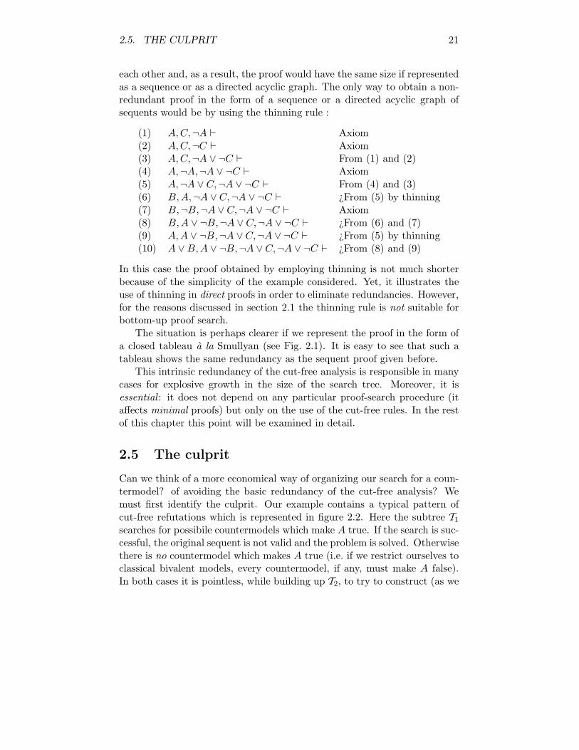
each other and, as a result, the proof would have the same size if representedas a sequence or as a directed acyclic graph. The only way to obtain a non-redundant proof in the form of a sequence or a directed acyclic graph ofsequents would be by using the thinning rule :
(1) A,C,¬A ⊢ Axiom(2) A,C,¬C ⊢ Axiom(3) A,C,¬A ∨ ¬C ⊢ From (1) and (2)(4) A,¬A,¬A ∨ ¬C ⊢ Axiom(5) A,¬A ∨ C,¬A ∨ ¬C ⊢ From (4) and (3)(6) B,A,¬A ∨ C,¬A ∨ ¬C ⊢ ¿From (5) by thinning(7) B,¬B,¬A ∨ C,¬A ∨ ¬C ⊢ Axiom(8) B,A ∨ ¬B,¬A ∨ C,¬A ∨ ¬C ⊢ ¿From (6) and (7)(9) A,A ∨ ¬B,¬A ∨ C,¬A ∨ ¬C ⊢ ¿From (5) by thinning(10) A ∨ B,A ∨ ¬B,¬A ∨ C,¬A ∨ ¬C ⊢ ¿From (8) and (9)
In this case the proof obtained by employing thinning is not much shorterbecause of the simplicity of the example considered. Yet, it illustrates theuse of thinning in direct proofs in order to eliminate redundancies. However,for the reasons discussed in section 2.1 the thinning rule is not suitable forbottom-up proof search.
The situation is perhaps clearer if we represent the proof in the form ofa closed tableau a la Smullyan (see Fig. 2.1). It is easy to see that such atableau shows the same redundancy as the sequent proof given before.
This intrinsic redundancy of the cut-free analysis is responsible in manycases for explosive growth in the size of the search tree. Moreover, it isessential : it does not depend on any particular proof-search procedure (itaffects minimal proofs) but only on the use of the cut-free rules. In the restof this chapter this point will be examined in detail.
2.5 The culprit
Can we think of a more economical way of organizing our search for a coun-termodel? of avoiding the basic redundancy of the cut-free analysis? Wemust first identify the culprit. Our example contains a typical pattern ofcut-free refutations which is represented in figure 2.2. Here the subtree T1
searches for possibile countermodels which make A true. If the search is suc-cessful, the original sequent is not valid and the problem is solved. Otherwisethere is no countermodel which makes A true (i.e. if we restrict ourselves toclassical bivalent models, every countermodel, if any, must make A false).In both cases it is pointless, while building up T2, to try to construct (as we

22 CHAPTER 2. THE REDUNDANCY OF CUT-FREE PROOFS
A ∨ B
A ∨ ¬B
¬A ∨ C
¬A ∨ ¬C
A
¬A
��� L
LLC
¬A
��� A
AA¬C
��
� ZZ
ZB
A
¬A
��� L
LLC
¬A
��� A
AA¬C
��� L
LL¬B
Figure 2.1: A closed tableau for {A ∨ B,A ∨ ¬B,¬A ∨ C,¬A ∨ ¬C}

2.6. SEARCHING FOR A COUNTERMODEL 23
T1
A is true
��
��
A ∨ ¬B is true
A ∨ B is true
...
@@
@@
B is true
T2
Figure 2.2: A typical pattern.
do if our search is governed by Gentzen’s rules) countermodels which makeA true, because this kind of countermodel is already sought in T1.
In general, we may have to reiterate this redundant pattern an arbitrarynumber of times, depending on the composition of our input set of formulae.For instance, if a branch contains n disjunctions A ∨ B1, . . . , A ∨ Bn whichare all to be analysed in order to obtain a closed subtableau, it is often thecase that the shortest tableau has to contain higly redundant configurationslike the one shown in figure 2.3: where the subtree T ∗ has to be repeatedn times. Each copy of T ∗ may, in turn, contain a similar pattern. It is notdifficult to see how this may rapidly lead to a combinatorial explosion whichis by no means related to any ‘intrinsic difficulty’ of the problem consideredbut only to the redundant behaviour of the cut-free rules.
2.6 Searching for a countermodel
The example discussed in sections 2.4 and 2.5 suggests that, in some sense,analytic tableaux constructed according to the cut-free tradition are notwell-suited to the nature of the problem they are intended to solve. In thissection we shall render this claim more precise.
Let us call a partial valuation of Γ, where Γ is a set of formulae, any partialfunction v : Γ 7→ {1, 0} where 1 and 0 stand as usual for the truth-valuestrue and false respectively. It is convenient for our purposes to representpartial functions as total functions with values in {1, 0, ∗} where ∗ standsfor the ‘undefined’ value. By a total valuation of Γ we shall mean a partial

24 CHAPTER 2. THE REDUNDANCY OF CUT-FREE PROOFS
...
A
T ∗
��� L
LLB1
A
T ∗
��� L
LLB2
A
T ∗
��� L
LLB3
...
Figure 2.3: Redundancy of tableau refutations.
valuation which for no element of Γ yields the value ∗. For every element Aof Γ we say that A is true under v if v(A) = 1, false under v if v(A) = 0 andundefined under v if v(A) = ∗. We say that a sequent Γ ⊢ ∆ is true underv if v(A) = 0 for some A ∈ Γ or v(A) = 1 for some A ∈ ∆. We say that itis false under v if v(A) = 1 for all A ∈ Γ and v(A) = 0 for all A ∈ ∆.
Let F denote the set of all formulae of propositional logic. A booleanvaluation, defined as usual, is regarded from this point of view as a specialcase of a partial valuation of F , namely one which is total and is faithful tothe usual truth-table rules.
In the no-countermodel approach to validity we start from a sequent Γ ⊢ ∆intended as a valuation problem and try to find a countermodel to it — at thepropositional level a boolean valuation which falsifies it. Here the direction ofthe procedure is characteristic: one moves from complex formulae to theircomponents in a typical ‘analytic’ way. In this context it is sufficient toconstruct some partial valuation which satisfies certain closure conditions.Such partial valuations have been extensively studied in the literature andare known under different names and shapes. They constitute the basic ideaunderlying the simple completeness proofs discovered in the ‘50’s which havebeen mentioned in the first two sections of this chapter. Following Prawitz[Pra74] we shall call them ‘semivaluations’:
Definition 2.6.1 Let Γ denote the closure of the set of formulae Γ under thesubformula relation. A (boolean) semivaluation of Γ is a partial valuation vof Γ which satisfies the following conditions:
1. if v(A ∨ B) = 1, then v(A) = 1 or v(B) = 1;

2.6. SEARCHING FOR A COUNTERMODEL 25
2. if v(A ∨ B) = 0, then v(A) = 0 and v(B) = 0;
3. if v(A ∧ B) = 1, then v(A) = 1 and v(B) = 1;
4. if v(A ∧ B) = 0, then v(A) = 0 or v(B) = 0;
5. if v(A → B) = 1, then v(A) = 0 or v(B) = 1;
6. if v(A → B) = 0, then v(A) = 1 and v(B) = 0;
7. if v(¬A) = 1, then v(A) = 0;
8. if v(¬A) = 0, then v(A) = 1.
The property of semivaluations which justifies their use is that they can bereadily extended to boolean valuations, i.e. models in the traditional sense:
Lemma 2.6.1 Every semivaluation of Γ can be extended to a boolean valu-ation.
Each stage of our attempt to construct a semivaluation which falsifies agiven sequent Γ ⊢ ∆ can, therefore, be described as a partial valuationv : Γ∪ ∆ 7→ {1, 0, ∗}. We start from the partial valuation which assigns 1 toall the formulae in Γ and 0 to all the formulae in ∆ and try to refine it byextending step by step its domain of definition, taking care that the classicalrules of truth are not infringed. If we eventually reach a partial valuationwhich is a semivaluation, we have successfully described a countermodel tothe original sequent. Otherwise we have to ensure that no way of refiningthe initial partial valuation will ever lead to a semivaluation.
The search space, then, is a set of partial valuations which are naturallyordered by the approximation relationship (in Scott’s sense [Sco70]):
v ⊑ v′ if and only if v(A) � v′(A) for all formulae A
where � is the usual partial ordering over {1, 0, ∗}, namely
∗@
@@
@
��
��
1 0

26 CHAPTER 2. THE REDUNDANCY OF CUT-FREE PROOFS
The set of all these partial valuations, together with the approximation re-lationship defined above, forms a complete semilattice. It can be convenientto transform this semilattice into a complete lattice by adding an ‘overde-fined’ element ⊤. This ‘fictitious’ element of the lattice does not correspondto any real partial valuation and is used to provide a least upper bound forpairs of partial valuations which have no common refinement19. Hence wecan regard the equation
v ⊔ v′ = ⊤
as meaning intuitively that v and v′ are inconsistent.Having described the primitive structure of the search space, we are left
with the problem of formulating efficient methods for exploring it. Con-structing an analytic tableau is one method and, as we will see, certainlynot the most efficient. This point is best seen by generalizing the basic ideaunderlying the tableau method. This is what will be done in the next twosubsections.
2.6.1 Expansion systems
We assume a 0-order language defined as usual. We shall denote by X,Y,Z(possibly with subscripts) arbitrary signed formulae (s-formulae), i.e. ex-pressions of the form t(A) or f(A) where A is a formula. The conjugate of ans-formula is the result of changing its sign (so t(A) is the conjugate of f(A)and viceversa). Sets of signed formulae will be denoted by S,U, V (possiblywith subscripts). We shall use the upper case greek letters Γ,∆, . . . for setsof unsigned formulae. We shall often write S,X for S ∪ {X} and S,U forS ∪U . Given a formula A, the set of its subformulae is defined in the usualway. We shall call subformulae of an s-formula s(A) (s = t, f) all the for-mulae of the form t(B) or f(B) where B is a subformula of A. For instancet(A), t(B), f(A), f(B) will all be subformulae of t(A ∨ B).
Definition 2.6.2 We say that an s-formula X is satisfied by a booleanvaluation v if X = t(A) and v(A) = 1 or X = f(A) and v(A) = 0. A set Sof s-formulae is satisfiable if there is a boolean valuation v which satisfies allits elements.
A set of s-formulae S is explicitly inconsistent if S contains both t(A)and f(A) for some formula A. If S is not explicitly inconsistent we say thatit is surface-consistent.
Sets of s-formulae correspond to the partial valuations of the previous sectionin the obvious way (we shall omit the adjective ‘partial’ from now on):
19Namely partial valuations v and v′ such that for some A in their common domain ofdefinition v(A) = 1 and v′(A) = 0.

2.6. SEARCHING FOR A COUNTERMODEL 27
given a surface-consistent set S of s-formulae its associated valuation is thevaluation vS defined as follows:
vS(A) =
1 if t(A) ∈ S0 if f(A) ∈ S∗ otherwise
(An explicitly inconsistent set of s-formulae is associated with the top el-ement ⊤.) Conversely, given a partial valuation v its associated set of s-formulae will be the set Sv containing t(A) for every formula A such thatv(A) = 1, and f(A) for every formula A such that v(A) = 0 (and nothingelse).
So we can always regard the s-formulae t(A) and f(A) as ‘meaning’v(A) = 1 and v(A) = 0 respectively.
The sets of s-formulae corresponding to semivaluations are known in theliterature as Hintikka sets.
Definition 2.6.3 A set of s-formulae S is a (propositional) Hintikka set ifit satisfies the following conditions (for every A,B):
1. For no variable P , t(P ) and f(P ) are both in S.
2. If t(¬A) ∈ S, then f(A) ∈ S.
3. If f(¬A) ∈ S, then t(A) ∈ S.
4. If t(A ∨ B) ∈ S, then t(A) ∈ S or t(B) ∈ S.
5. If f(A ∨ B) ∈ S, then f(A) ∈ S and f(B) ∈ S.
6. If t(A ∧ B) ∈ S, then t(A) ∈ S and t(B) ∈ S.
7. If f(A ∧ B) ∈ S, then f(A) ∈ S or f(B) ∈ S.
8. If t(A → B) ∈ S, then f(A) ∈ S or t(B) ∈ S.
9. If f(A → B) ∈ S, then t(A) ∈ S and f(B) ∈ S.
The sets of s-formulae corresponding, in a similar way, to a boolean valuationare often called truth sets or saturated sets. The translation of lemma 2.6.1is known as the (propositional) Hintikka lemma.
Lemma 2.6.2 (Propositional Hintikka lemma) Every propositional Hin-tikka set is satisfiable.

28 CHAPTER 2. THE REDUNDANCY OF CUT-FREE PROOFS
In other words, every Hintikka set can be embedded in a truth set.We shall now define the notion of expansion system which generalizes
the tableau method.
Definition 2.6.4
1. An n×m expansion rule R is a relation between n-tuples of s-formulaeand m-tuples of s-formulae, with n ≥ 0 and m ≥ 1. Expansion rulesmay be represented as follows:
χ1...
χn
υ1| . . . |υm
where the χi’s and the υi’s are schemes of s-formulae. We say that therule has n premises and m conclusions. If m = 1 we say that the ruleis of linear type, otherwise we say that the rule is of branching type.
2. An expansion system S is a finite set of expansion rules.
3. We say that S,X is an expansion of S under an n×m rule R if thereis an n-tuple a of elements of S such that X belongs to some m-tupleb in the set of the images of a under R.
4. Let R be an n × m expansion rule. A set U is saturated under R orR-saturated, if for every n-tuple a of elements of U and every m-tupleb in the set of the images of a under R, at least one element of b isalso in U .
5. A set U is S-saturated if it is R-saturated for every rule R of S.
The rules of an expansion system are to be read as rules which allow us toturn a tree of s-formulae into another such tree. Suppose we have a finitetree T and φ is one of its branches. Let R be an n × m expansion rule and(Y1, . . . , Ym) an image under R of some n-tuple of s-formulae occurring in φ.Then we can extend T by appending m immediate successors (Y1, . . . , Ym)(in different branches) to the end of φ. Let us call T ′ the result. We saythat T ′ results from T by an application of R.
We also say that the application of R is analytic if it has the subformulaproperty, i.e. all the new s-formulae appended to the end of φ are subformulaeof s-formulae occurring in φ. A rule R is analytic if every application of Ris analytic (i.e. all the conclusions are subformulae of the premises).

2.6. SEARCHING FOR A COUNTERMODEL 29
We can then use an expansion system S to give a recursive definition ofthe notion of (analytic) S-tree for S, where S is a finite set of s-formulae.
Definition 2.6.5 Let S = {X1, . . . ,Xn}.
1. The following one branch tree is an (analytic) S-tree for S:
X1
X2...
Xn
2. If T is an (analytic) S-tree for S and T ′ results from T by an (analytic)application of an expansion rule of S, then T ′ is also an (analytic) S-tree for S.
3. Nothing else is an (analytic) S-tree for S.
Let φ be a branch of an S-tree. We say that φ is closed if the set of itsnodes is explicitly inconsistent. Otherwise it is open. A tree T is closed ifall its branches are closed and open otherwise. We also say that a branch φis complete if it is closed or the set of its nodes is S-saturated. A tree T iscompleted if all its branches are complete.
As far as this chapter is concerned we are interested in expansion systemswhich represent (analytic) refutation systems for classical propositional logic,i.e. systems S such that, for every finite set of s-formulae S, S is classicallyunsatisfiable if and only if there is a closed S-tree for S.
2.6.2 Redundant trees
Any set of rules meeting our definition of analytic refutation system can beconsidered an adequate formalization of the idea of proving validity by afailed attempt to construct a countermodel. Each expansion step in such asystem reduces a problem concerning a set S (is S satisfiable?) to a finite setof ‘easier’ subproblems of the same kind concerning supersets of S. Thinkingin terms of partial valuations, each step yields a finite set of more accurateapproximations to the sought-for semivaluation(s).
However, we have observed that the search space has a natural structureof its own. It is therefore reasonable to require that the rules we adopt inour systematic search reflect this structure. This can be made precise asfollows: given an S-tree T we can associate with each node n of T , the setof the s-formulae occurring in the path from the root to n or, equivalently,

30 CHAPTER 2. THE REDUNDANCY OF CUT-FREE PROOFS
the partial valuation vn which assigns 1 to all the formulae A such that t(A)occurs in the path to n, and 0 to all the formulae A such that f(A) occursin the path to n (and leaves all the other formulae undefined). We can thenrequire that the relations between the nodes in an S-tree correspond to therelations between the associated partial valuations.
Definition 2.6.6 Let T be an S-tree and let �T the partial ordering definedby T on the set of its nodes (i.e. for all nodes n1, n2, n1 �T n2 if an only if n1
is a predecessor of n2). We say that a refutation system S is non-redundantif the following condition is satisfied for every S-tree T and every pair n1, n2
of nodes of T :n1 �T n2 ⇐⇒ vn1
⊑ vn2.
Non-redundancy as defined above seems a very natural requirement on refu-tation systems: we essentially ask that our refutation system generate treeswhich follow the structure of the approximation problems they set out tosolve. (Notice that the only-if part of the condition is trivial, but the ifpart is not so trivial.) One corollary of non-redundancy, which justifies thischoice of terminology, is the following: let us say that an S-tree T is redun-dant if for some pair of nodes n1, n2 belonging to different branches of T ,we have that vn1
⊑ vn2. Such a tree is obviously redundant for the reasons
discussed in section 2.5: if vn1can be extended to a semivaluation, we have
found a countermodel to the original sequent and the problem is solved.Otherwise, if no extension of vn1
is a semivaluation, the same applies to vn2.
It immediately follows from our definitions that:
Corollary 2.6.1 If S is a non-redundant system, no S-tree is redundant.
The importance of non-redundancy for a system is both conceptual andpractical. A redundant tree does not reflect the structure of the semanticspace of partial valuations which it is supposed to explore and this veryfact has disastrous computational consequences: redundant systems are ill-designed, from an algorithmic point of view, in that, in some cases, they forceus to repeat over and over again what is essentially the same computationalprocess.
It is easy to see that the non-redundancy condition is not satisfied bythe tableau method (and in general by cut-free Gentzen systems). We cantherefore say that, in some sense, such systems are not natural for classicallogic20.
20This suggestion may be contrasted with Prawitz’s suggestion, advanced in [Pra74],that ‘Gentzen’s calculus of sequents may be understood as the natural system for gener-ating logical truths’.

Chapter 3
An alternative approach
3.1 Bivalence restored
The main feature of the tableau method and of all the variants of Gentzen’scut-free systems is the close correspondence between their rules and theclauses of the semantic definition of semivaluation1. This is the reason thatsuch systems are usually regarded as ‘natural’. But, as we have argued,the tree-structure generated by the semivaluation clauses bears a tortuousrelation to the structure of the space of partial valuations, i.e. the partialsemantic objects by which we represent our successive approximations tothe sought-for countermodel. So, our non-redundancy condition suggeststhat we should not use such clauses as rules in our search.
Is there a simple way out? There is. We need only to take into consid-eration that models, or countermodels, in classical logic, are bivalent. Asseen is section 2.3, this crucial piece of semantic information is hidden bythe cut-free Gentzen rules. So in order to establish a close correspondencebetween formal derivability and classical semantics we have to reintroducethe notion of bivalence in our analysis. It will transpire that this is in factall we need to do.
The non-redundancy condition given in definition 2.6.6 is automatically sat-isfied by any refutation system S which satisfies the stronger condition that,for all S-trees T and all nodes n1, n2
n1 6�T n2 and n2 6�T n1 =⇒ vn1⊔ vn2
= ⊤(3.1)
i.e., any two different branches define inconsistent partial valuations.
1This correspondence is discussed thoroughly in [Pra74].
31

32 CHAPTER 3. AN ALTERNATIVE APPROACH
It is obvious that the only rule of the branching type which generatestrees with this property is a 0-premise rule, corresponding to the principleof bivalence:
t(A)�
��
�@@
@@f(A)
So our discussion strongly suggests that the principle of bivalence should bere-introduced in some way as a rule in the search for a countermodel andthat, indeed, it should be the only ‘branching’ rule to govern this search.
Three problems immediately arise in connection with the use of PB in arefutation system:
1. Are there simple analytic rules of linear type which combined with PByield a refutation system for classical logic?
2. Since a 0-premise rule like PB can introduce arbitrary formulae, canwe restrict ourselves to analytic applications of PB without affectingcompleteness?
3. Even if the previous question has a positive answer, we shall be leftwith a large choice of formulae to introduce via PB. This could be aproblem from a practical point of view. Can we further restrict thischoice?
The rest of this chapter will be devoted to studying an alternative approachbased on the system KE, recently proposed in [Mon88a, Mon88b], whichgives our three questions positive answers.
3.2 The system KE
Let us consider the case in which, at a certain point of the search tree, weexamine a partial function which renders a disjunction, A ∨ B, true. Then,instead of applying the tableau branching rule as in the left diagram offigure 3.1, we apply the rule PB as in the diagram on the right2. Next, we
2In this example we apply PB to the formula A. A similar configuration is obtainedby applying PB to the formula B. We need only one of these applications. Although thechoice of the formula does not affect completeness, it may affect the complexity of theresulting refutation. See below p. 72.

3.2. THE SYSTEM KE 33
t(A ∨ B)
��
��
@@
@@
t(A) t(B)
t(A ∨ B)
��
��
@@
@@
t(A) f(A)
t(B)
Figure 3.1: Two different analyses.
observe that any boolean valuation which makes A ∨ B true and A falsemust make B true.
If we compare the result of this way of analysing the disjunction with theresult of applying the tableau branching rule, we notice that (i) the lefthandbranch represents the same partial valuation, but (ii) the partial valuationrepresented by the righthand branch is more defined, i.e. contains more in-formation: precisely the information that if A is not true, it must be false;so if there are no countermodels which make A true, every countermodel, ifany, must make A false. We can then use this information to exclude fromthe search space associated with the righthand branch all the partial valua-tions which make A true, whereas such partial valuations are not excludedif we apply the standard tableau rule. In other words, our chances of closingbranches are significantly increased.
The example suggests that we can find a set of rules of the linear type which,combined with PB, provides a complete refutation system for propositionallogic. We need only to notice that the following eleven facts hold true (forany formulae A,B) under any boolean valuation:
1. If A ∨ B is true and A is false, then B is true.
2. If A ∨ B is true and B is false, then A is true.
3. If A ∨ B is false then both A and B are false.
4. If A ∧ B is false and A is true, then B is false.
5. If A ∧ B is false and B is true, then A is false.

34 CHAPTER 3. AN ALTERNATIVE APPROACH
6. If A ∧ B is true then both A and B are true.
7. If A → B is true and A is true, then B is true.
8. If A → B is true and B is false, then A is false.
9. If A → B is false, then A is true and B is false.
10. If ¬A is true, then A is false.
11. If ¬A is false, then A is true.
These facts can immediately be used to provide a set of expansion rulesof the linear type which, with the addition of PB, correspond to the thepropositional fragment of the system KE proposed in [Mon88a, Mon88b].The rules of KE are shown below. Notice that those with two s-formulaebelow the line represent a pair of expansion rules of the linear type, one foreach s-formula.
Disjunction Rules
t(A ∨ B)f(A)
t(B)Et∨1
t(A ∨ B)f(B)
t(A)Et∨2
f(A ∨ B)
f(A)f(B)
Ef∨
Conjunction Rules
f(A ∧ B)t(A)
f(B)Ef∧1
f(A ∧ B)t(B)
f(A)Ef∧2
t(A ∧ B)
t(A)t(B)
Et∧
Implication Rules
t(A → B)t(A)
t(B)Et →1
t(A → B)f(B)
f(A)Et →2
f(A → B)
t(A)f(B)
Ef →
Negation Rules
t(¬A)
f(A)Et¬
f(¬A)
t(A)Ef¬
3.2. THE SYSTEM KE 35
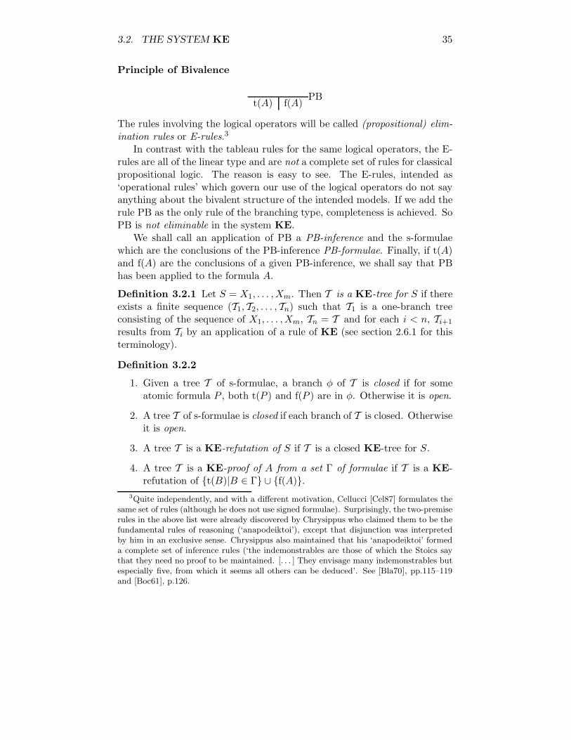
Principle of Bivalence
t(A) f(A)PB
The rules involving the logical operators will be called (propositional) elim-ination rules or E-rules.3
In contrast with the tableau rules for the same logical operators, the E-rules are all of the linear type and are not a complete set of rules for classicalpropositional logic. The reason is easy to see. The E-rules, intended as‘operational rules’ which govern our use of the logical operators do not sayanything about the bivalent structure of the intended models. If we add therule PB as the only rule of the branching type, completeness is achieved. SoPB is not eliminable in the system KE.
We shall call an application of PB a PB-inference and the s-formulaewhich are the conclusions of the PB-inference PB-formulae. Finally, if t(A)and f(A) are the conclusions of a given PB-inference, we shall say that PBhas been applied to the formula A.
Definition 3.2.1 Let S = X1, . . . ,Xm. Then T is a KE-tree for S if thereexists a finite sequence (T1,T2, . . . ,Tn) such that T1 is a one-branch treeconsisting of the sequence of X1, . . . ,Xm, Tn = T and for each i < n, Ti+1
results from Ti by an application of a rule of KE (see section 2.6.1 for thisterminology).
Definition 3.2.2
1. Given a tree T of s-formulae, a branch φ of T is closed if for someatomic formula P , both t(P ) and f(P ) are in φ. Otherwise it is open.
2. A tree T of s-formulae is closed if each branch of T is closed. Otherwiseit is open.
3. A tree T is a KE-refutation of S if T is a closed KE-tree for S.
4. A tree T is a KE-proof of A from a set Γ of formulae if T is a KE-refutation of {t(B)|B ∈ Γ} ∪ {f(A)}.
3Quite independently, and with a different motivation, Cellucci [Cel87] formulates thesame set of rules (although he does not use signed formulae). Surprisingly, the two-premiserules in the above list were already discovered by Chrysippus who claimed them to be thefundamental rules of reasoning (‘anapodeiktoi’), except that disjunction was interpretedby him in an exclusive sense. Chrysippus also maintained that his ‘anapodeiktoi’ formeda complete set of inference rules (‘the indemonstrables are those of which the Stoics saythat they need no proof to be maintained. [. . . ] They envisage many indemonstrables butespecially five, from which it seems all others can be deduced’. See [Bla70], pp.115–119and [Boc61], p.126.

36 CHAPTER 3. AN ALTERNATIVE APPROACH
5. A is KE-provable from Γ if there is a KE-proof of A from Γ.
6. A is a KE-theorem if A is KE-provable from the empty set of formulae.
Remark: it is easy to prove that if a branch φ of T contains both t(A)and f(A) for some formula A (not necessarily atomic), φ can be extendedby means of the E-rules only to a branch φ′ which is closed in the sense ofthe previous definition. Hence, in what follows we shall consider a branchclosed as soon as both t(A) and f(A) appear in it.
As pointed out in Section 2.3, there is a close correspondence between thesemantic rule PB and the cut rule of the sequent calculus. We shall returnto this point in Section 4.5.2.
We can give a version of KE which works with unsigned formulae. Therules are shown in Table 3.1. It is intended that all definitions be modifiedin the obvious way.
We can see from the unsigned version that the two-premise rules corre-spond to well-known principles of inference: modus ponens, modus tollens,disjunctive syllogism and the dual of disjunctive syllogism. This gives KEa certain natural-deduction flavour (see Section 3.8). However, the clas-sical operators are analysed as such and not as ‘stretched’ versions of theconstructive ones.
In Fig. 3.2 we give a KE-refutation (using unsigned formulae) of thesame set for which a minimal tableau was given on p. 22; the reader cancompare the different structure of the two refutations and the crucial use of(the unsigned version of) PB to eliminate the redundancy exhibited by thetableau refutation.
3.3 Soundness and completeness of KE
We shall give the proofs for KE-trees using signed formulae. The modifica-tions for KE-trees using unsigned formulae are obvious.
Proposition 3.3.1 (Soundness of KE) If there is a closed KE-tree forS, then S is unsatisfiable.
Proof. The proof is essentially the same as the soundness proof for thetableau method. See [Smu68a, p. 25].
The completeness of KE can be shown in several ways. One is by prov-ing that the set of KE-theorems includes some standard set of axioms forpropositional logic and is closed under modus ponens. Another way is by

3.3. SOUNDNESS AND COMPLETENESS OF KE 37
Disjunction Rules
A ∨ B
¬A
BE∨1
A ∨ B
¬B
AE∨2
¬(A ∨ B)
¬A
¬B
E¬∨
Conjunction Rules
¬(A ∧ B)A
¬BE¬∧1
¬(A ∧ B)B
¬AE¬∧2
A ∧ B
A
B
E∧
Implication Rules
A → B
A
BE→1
A → B
¬B
¬AE→2
¬(A → B)
A
¬B
E¬ →
Negation Rule
¬¬A
AE¬¬
Principle of Bivalence
A ¬APB
Table 3.1: KE rules for unsigned formulae.

38 CHAPTER 3. AN ALTERNATIVE APPROACH
×
¬B
B
¬A
×
¬C
C
¬¬A
��
��
@@
@@
¬A ∨ ¬C
¬A ∨ C
A ∨ ¬B
A ∨ B
Figure 3.2: A KE-refutation of {A ∨ B,A ∨ ¬B,¬A ∨ C,¬A ∨ ¬C}
modifying the traditional completeness proof for the tableau method. Weshall give both these proofs because they provide us with different kindsof information. (One can also obtain a proof a la Kalmar [Kal34]. See[Mon88a].)
3.3.1 Completeness of KE: proof one
Theorem 3.3.1 If A is a valid formula than there is a KE-proof of A.
Proof. The theorem immediately follows from the following facts whichat the same time provide examples of KE-refutations (we write just ⊢ for⊢KE):
Fact 3.3.1 ⊢ A → (B → A)
f(A → (B → A))
t(A)f(B → A)t(B)f(A)×

3.3. SOUNDNESS AND COMPLETENESS OF KE 39
Fact 3.3.2 ⊢ (A → (B → C)) → ((A → B) → (A → C))
f((A → (B → C)) → ((A → B) → (A → C)))
t(A → (B → C))f((A → B) → (A → C))t(A → B)f(A → C)t(A)f(C)t(B → C)f(B)t(B)×
Fact 3.3.3 ⊢ (¬B → ¬A) → (A → B)
f((¬B → ¬A) → (A → B))
t(¬B → ¬A)f(A → B)
t(A)f(B)
t(¬B) | f(¬B)t(¬A) t(B)f(A) ××
Fact 3.3.4 If ⊢ A and ⊢ A → B, then ⊢ B
Proof. It follows from the hypothesis that there are refutations T1 and T2
respectively of {f(A)} and {f(A → B)}. Then the following tree:
f(B)
t(A → B) | f(A → B)f(A) T2
T1
is a refutation of {f(B)}.2
This kind of proof provides a simulation of a standard axiomatic system.

40 CHAPTER 3. AN ALTERNATIVE APPROACH
In this simulation it is essential to apply the rule PB to formulae whichare not subformulae of the theorem to be proved. We notice that such asimulation cannot be directly obtained by the tableau method, since it isnon-analytic. Are such non-analytic applications of PB necessary or can theybe eliminated without loss of completeness? i.e. can we restrict ourselves toanalytic applications? Let us say that a KE-tree T for Γ is analytic if PBis applied in T only to (proper) subformulae of formulae in Γ. Let us callKE∗ the analytic restriction of KE, i.e. the system in which the applicationsof PB are restricted to subformulae of the formulae occurring above in thesame branch. So our problem becomes: is KE∗ complete?
A positive answer to this question can be obtained from the second com-pleteness proof which follows the lines traced by Beth [Bet55] and Hintikka[Hin55]. This proof not only ensures that we can restrict ourselves to an-alytic applications of PB so that our refutations will obey the subformulaprinciple, but also provides more information concerning the formulae to beconsidered in these applications.
3.3.2 Completeness of KE: proof two
It is convenient to use Smullyan’s unifying notation in order to reduce thenumber of cases to be considered.
We use the letter ‘α’ to stand for any signed formula of one of the forms:t(A ∧ B), f(A ∨ B), f(A → B), t(¬A), f(¬A).
For every such formula α, its components α1 and α2 are defined as in thefollowing table:
α α1 α2
t(A ∧ B) t(A) t(B)
f(A ∨ B) f(A) f(B)
f(A → B) t(A) f(B)
t(¬A) f(A) f(A)
f(¬A) t(A) t(A)
We use ‘β’ to stand for any formula of one of the forms: f(A∧B), t(A∨B),t(A → B). For every such formula β, its components β1 and β2 are definedas in the following table:
β β1 β2
f(A ∧ B) f(A) f(B)
t(A ∨ B) t(A) t(B)
t(A → B) f(A) t(B)

3.3. SOUNDNESS AND COMPLETENESS OF KE 41
So the E-rules of KE can be ‘packed’ into the following three rules (whereβ′
i, i = 1, 2 denotes the conjugate of βi):
Rule A
α
α1
α2
Rule B1
ββ′
1
β2
Rule B2
ββ′
2
β1
Remarks. The unifying notation can be easily adapted to unsigned for-mulae: simply delete all the signs ‘t’ and replace all the signs ‘f’ by ‘¬’.The ‘packed’ version of the rules then suggests a more economical versionof KE for unsigned formulae when β′
i is taken to denote the complement ofβi defined as follows: the complement of an unsigned formula A, is equal to¬B if A = B and to B if A = ¬B. In this version the rules E∨1, E∨2 andE→2 become:
A ∨ BA′
B
A ∨ BB′
C
A → BB′
A′
This version is to be preferred for practical application. Notice also that theRule A represents a pair of expansion rules, one with conclusion α1 and theother with conclusion α2.
In each application of the rules, the signed formulae α and β are called majorpremises. In each application of rules B1 and B2 the signed formulae β′
i,i = 1, 2 are called minor premises (rule A has no minor premise).
We first define a notion akin to that of a Hintikka set:
Definition 3.3.1 Let us say that a set of s-formulae S is a propositionalanalytic set if and only if it satisfies the following conditions:
A0: For no atomic formula P , t(P ) and f(P ) are both in S.
A1: If α ∈ S, then α1 ∈ S and α2 ∈ S.
A2: If β ∈ S and β′1 ∈ S, then β2 ∈ S.
A3: If β ∈ S and β′2 ∈ S, then β1 ∈ S.

42 CHAPTER 3. AN ALTERNATIVE APPROACH
An analytic set differs from a Hintikka set in that it may be the case thatfor some β in the set neither β1 nor β2 is in the set.
Definition 3.3.2 We say that an analytic set S is β-complete if for everyβ in S one of the following two conditions is satisfied:
Ba: either β1 ∈ S or β′1 ∈ S;
Bb: either β2 ∈ S or β′2 ∈ S.
It is then easy to verify that:
Fact 3.3.5 If S is a propositional analytic set and S is β-complete, then Sis a propositional Hintikka set.
Let us say that a branch φ of a KE-tree is E-complete if the set Sφ of thes-formulae occurring in it is saturated under the E-rules of KE. Let us alsosay that φ is β-complete if for every formula of type β occurring in it andsome i = 1, 2, either βi or β′
i occurs in φ. We say that φ is complete if it isE-complete and β-complete. Finally, we say that a KE-tree T is completedif every branch of T is either closed or complete. Of course if φ is an openbranch in a completed KE-tree, the set Sφ of its s-formulae is a β-completeanalytic set and, hence, a Hintikka set.
Thus, completeness follows from fact 3.3.5 and the propositional Hintikkalemma.
Theorem 3.3.2 (Completeness Theorem) If Γ |= A, then there is aclosed KE-tree for {t(B)|B ∈ Γ} ∪ {f(A)}. In particular every completedKE-tree is closed.
3.3.3 The subformula principle
Our proof of the completeness of KE yields the subformula principle as acorollary. Since all the rules except PB are analytic, we need only to observethat the completeness proof given above immediately implies:
Corollary 3.3.1 (Analytic cut property) If S is unsatisfiable, then thereis a closed KE-tree T ′ for S such that all the applications of PB are analytic.Equivalently, the analytic restriction of KE is complete.
A constructive proof of the subformula principle, which yields a procedurefor transforming any KE-proof in an equivalent KE-proof which enjoys thesubformula property, is given in [Mon88b].
Our completeness proof also gives us some additional information. Let us

3.3. SOUNDNESS AND COMPLETENESS OF KE 43
say that a formula of type β is analysed in a branch φ if either β1 or β2
occurs in φ. An application of PB in a branch φ of a KE-tree is canonical ifthe s-formulae of this application are βi and β′
i for some i = 1, 2 and somenon-analysed formula of type β occurring in φ. A KE-tree is canonical if itcontains only canonical applications of PB. It follows from our completenessproof that
Corollary 3.3.2 If S is unsatisfiable, then there is a closed canonical KE-tree for S.
In other words, our proof establishes the completeness of the restricted sys-tem KE′ obtained by replacing the ‘liberal’ version of PB with one whichallows only canonical applications.
There are several procedures which, given a finite or denumerable set ofsigned formulae S, generate a completed (canonical) KE-tree. Here is onepossibility (adapted from [Smu68a, [pp. 33–34]). Let us say that a node isfulfilled if (1) it is an atomic s-formula or (2) it is of type α and both α1 andα2 occur in all the branches passing through the node or (3) it is of typeβ and for every branch φ passing through the node all the following threeconditions are satisfied: (3a) if β′
1 occurs in φ, β2 also occurs in φ; (3b) if β′2
occurs in φ, β1 also occurs in φ; (3c) for some i = 1, 2 either βi or β′i occurs
in φ. Obviously a KE-tree is completed if and only if every node is fulfilled.We can now describe a simple procedure to construct a completed KE-
tree for every denumerable set of s-formulae. Let S be arranged in a denu-merable sequence X1,X2, . . .. Start the tree with X1. This node constitutesthe level 1. Then fulfil4 the origin and append X2 to every open branch.Call all the nodes so obtained nodes of level 2. At the i-th step fulfil allthe nodes of level i − 1 and append Xi to the end of each open branch. Soevery node gets fulfilled after a finite number of steps. The procedure eitherterminates with a closed KE-tree or runs forever. (If S is finite, the proce-dure always terminates). In this case we ‘obtain’ an infinite tree which isa completed KE-tree for S. Since the tree is finitely generated, by Konig’slemma it must contain an infinite branch which is obviously open. The setof s-formulae in this branch is a Hintikka set. Therefore S is satisfiable. IfS is unsatisfiable the procedure generates a finite tree.
The procedure just described is a simple variant of a similar procedurebased on the tableau method which is used to provide (among other things)a proof of the compactness theorem. Our adaptation is an example of howall the useful theoretical properties of cut-free systems can be almost imme-diately transferred to a system like KE which is not cut-free.
4By ‘fulfilling a node’ we mean applying the KE-rules so that the node becomes fulfilled.

44 CHAPTER 3. AN ALTERNATIVE APPROACH
Remark. Like the tableau method, KE (with PB restricted to canonicalapplications) can be used as a method for turning arbitrary formulae intodisjunctive normal form. However, the DNFs obtained by means of thetableau method may often be highly redundant and contain a number ofconjunctions which are subsumed by other conjunctions (a conjunction C1
subsumes another conjunction C2, if all the literals occurring in C1 occuralso in C2). By contrast the DNFs obtained by means of KE are in mostcases remarkably concise. The dual versions of the rules (i.e. the rules ob-tained from rules A, B1 and B2 by swapping α and β) provide a method forturning an arbitrary formula into conjunctive (or ‘clausal’) normal form.
¬¬A
A
β
β1
β2
αα′
1
α2
αα′
2
α1A ¬A
Table 3.2: CNF reduction rules.
Again, the CNFs yielded by this method are in most cases much moreconcise than those yielded by the analogous dual version of the tableaumethod (see [Fit90, p. 26]). It is a consequence of results in Section 4.5.2that in the worst case the number of (disjunctions) conjunctions in theshortest5 normal form of A yielded by the (duals of the) tableau rules is noteven polynomially related to the corresponding number of (disjunctions)conjunctions yielded by the (duals of the) KE rules. By contrast the (dualsof the) KE rules never yield normal forms which are longer than thoseyielded by the (duals of the) tableau rules.
3.4 KE and the Davis-Putnam Procedure
The Davis-Putnam procedure was introduced in 1960 [DP60] and later re-fined in [DLL62]. It was meant as an efficient theorem proving method6
for (prenex normal form) first-order logic, but it was soon recognized that itcombined an efficient test for truth-functional validity with a wasteful searchthrough the Herbrand universe7. This situation was later remedied by theemergence of unification. However, at the propositional level, the procedureis still considered among the most efficient, and is clearly connected with theresolution method, so that Robinson’s resolution [Rob65] can be viewed as a
5That is to say, we consider the non-deterministic version of the algorithm.6The version given in [DP60] was not in fact a completely deterministic procedure: it
involved the choice of which literal to eliminate at each step.7See [Dav83].

3.4. KE AND THE DAVIS-PUTNAM PROCEDURE 45
A1 ∨ . . . ∨ An
A′i
(A1 ∨ . . . ∨ An) \ Ai
¬(A1 ∧ . . . ∧ An)Ai
¬((A1 ∧ . . . ∧ An) \ Ai)
¬(A1 ∨ . . . ∨ An)
¬A1...
¬An
A1 ∧ . . . ∧ An
A1...
An
Table 3.3: Generalized KE rules.
(non-deterministic) combination of the Davis-Putnam propositional moduleand unification, in a single inference rule. It is not difficult to see that, ifwe extend our language to deal with ‘generalized’ disjunctions and conjunc-tions, the Davis-Putnam procedure (in the version of [DLL62] which is alsothe one exposed in [CL73, Section 4.6] and in Fitting’s recent book [Fit90,Section 4.4]), can be represented as a special case of the canonical procedurefor KE outlined in the previous section. So, from this point of view, KEprovides a generalization of the Davis-Putnam procedure which does notrequire reduction in clausal form.
We enrich our language to include expression of the form A1 ∨ . . . ∨ An
and A1 ∧ . . . ∧ An, where A1, . . . , An are formulae, and use the notationA1 ◦ . . . ◦ An \ Ai, where ◦ is ∨ or ∧, i = 1, . . . , n, to denote the result ofremoving Ai from A1 ◦ . . . ◦ An. We then replace the rules E∨i, E¬ ∧ i,i = 1, 2, E¬∨, E∧ of KE with the generalized versions shown in Table 3.3(we use the notation A′ for the complement of A).
We can generalize Smullyan’s notation to cover the new language includ-ing n-ary conjunctions and disjunctions: use the notation αn for an n-aryconjunction or the negation of an n-ary disjunction, and the notation βn foran n-ary disjunction or the negation of an n-ary conjunction (or an n-aryimplication A1 → (. . . (An−1 → An) . . .)). The components αn
i and βni , for
i = 1, . . . , n are defined in the obvious way. The notation βn\i, i = 1, . . . , nis used as follows:
βn\i =
{(A1 ∨ . . . ∨ An) \ Ai if βn = A1 ∨ . . . ∨ An
¬((A1 ∨ . . . ∨ An) \ Ai) if βn = ¬(A1 ∧ . . . ∧ An)
Let us consider now the procedure given in the previous section and replace

46 CHAPTER 3. AN ALTERNATIVE APPROACH
the definition of fulfilled node as follows: let us say that a node is fulfilledif (1′) it is a literal or (2′) it is of type αn and, for every i = 1, . . . , n, αn
i
occurs in all the branches passing through the node or (3′) it is of type βn
and for every branch φ passing through the node all the following conditionsare satisfied: (3′a) if βn
i′ occurs in φ, βn\i also occurs in φ; (3′b) for some
i = 1, 2, . . . , n either βni or βn
i′ occurs in φ.
It is not difficult to see that the same procedure described in the previoussection is complete for this extended language. Moreover, if we restrict ourattention to formulae in CNF and add two simplification rules correspondingto the ‘affirmative-negative’ rule and to the ‘subsumption rule’ (see [DLL62]and [Fit90]), the procedure becomes equivalent to the Davis-Putnam pro-cedure. So KE incorporates the basic idea underlying resolution theoremproving in a tableau-like set up. From this point of view it is somehowrelated to non-clausal resolution [Mur82, MW80].
We also notice that the system resulting from this generalized versionof KE by disallowing the branching rule PB includes, as a special case, therestriction of resolution known as unit resolution [Cha70]. This restrictedversion of KE can then be seen as an extension of unit resolution (it is there-fore a complete system for Horn clauses, although its scope is not confinedto formulae in clausal form).
3.5 The first-order system KEQ
In this section we consider a standard first-order language with no func-tional symbols. We use the letters x, y, z, . . . (possibly with subscripts) asindividual variables and the letters a, b, c, . . . (possibly with subscripts) asparameters. For any variable x and parameter a, A(x/a) will be the resultof substituting all the free occurrences of x in A with a. Subformulae are de-fined in the usual way, so that for every parameter a, A(x/a) is a subformulaof ∀xA(x).
The rules of the first-order system KEQ consist of the rules of thepropositional fragment (with the obvious assumption that the metavari-ables range over closed first-order formulae) plus the quantifier rules of thetableau method, namely:
Universal Quantifier Rules
t((∀x)A)
t(A(x/a))Et∀
f((∀x)A)
f(A(x/a))Ef∀ with a new

3.6. SOUNDNESS AND COMPLETENESS OF KEQ 47
Existential Quantifier Rules
f((∃x)A)
f(A(x/a))Ef∃
t((∃x)A)
t(A(x/a))Et∃ with a new
The versions for unsigned formulae are obtained, as before, by changing thesign f into ‘¬’ and deleting the sign t.
We shall use Smullyan’s unifying notation for first-order formulae. For-mulae of type α and β are defined as in the propositional case (except thatformulae here means closed first-order formulae). In addition we use γ todenote any formula of one of the forms t(∀xA(x)), f(∃xA(x)), and by γ(a)we shall mean, respectively, t(A(x/a)), f(A(x/a)). Similarly δ will denoteany formula of one of the forms t(∃xA(x)), f(∀xA(x)) and by δ(a) we shallmean, respectively, t(A(x/a)), f(A(x/a)).
Using the unifying notation the quantifier rules are:
Rule Cγ
γ(a) for any parameter a
Rule Dδ
δ(a) for a new parameter a
3.6 Soundness and completeness of KEQ
The first-order system KEQ is obviously sound for the same reasons as thetableau method. It is easy to extend the first completeness proof given forthe propositional fragment in section 3.3.1. We just need to observe thatthe set of KEQ-theorems is closed under the standard quantifier rules of afirst-order axiomatic system.
Fact 3.6.1 If ⊢KEQ A → B(a) and a does not occur in A, then⊢KEQ A → (∀x)B(a/x)
Fact 3.6.2 If ⊢KEQ B(a) → A and a does not occur in A, then⊢KEQ (∃x)B → A.
The second completeness proof given in section 3.3.2 can also be readilyextended to the first-order system.
We recall the notion of first-order Hintikka set.
Definition 3.6.1 By a first-order Hintikka set (for a universe U) we mean aset S of s-formulae (with constants in U) such that the following conditionsare satisfied for every α, β, γ, δ over U :

48 CHAPTER 3. AN ALTERNATIVE APPROACH
H0: No signed variable and its complement are both in S.
H1: If α ∈ S, then α1 ∈ S and α2 ∈ S.
H3: If β ∈ S, then β1 ∈ S or β2 ∈ S.
H4: If γ ∈ S, then for every a in U , γ(a) ∈ S.
H5: If δ ∈ S, then for some a in U , δ(a) ∈ S.
The notion of first-order analytic set over U is the analogous extension ofthe propositional notion:
Definition 3.6.2 By a first-order analytic set (for a universe U we mean aset S of s-formulae (with constants in U) such that the following conditionsare satisfied for every α, β, γ, δ over U :
A0: No signed variable and its complement are both in X.
A1: If α ∈ S, then α1 ∈ S and α2 ∈ S.
A2: If β ∈ S and β′1 ∈ S, then β2 ∈ S.
A3: If β ∈ S and β′2 ∈ S, then β1 ∈ S.
A4: If γ ∈ S, then for every a in U , γ(a) ∈ X.
A5: If δ ∈ S, then for some a in U , δ(a) ∈ S.
Again we observe that if S is a first-order analytic set and S is β-complete,S is a first-order Hintikka set.
It is not difficult to define a procedure which, given a set of s-formulaeS, generates either a (canonical) closed KEQ-tree or an open KEQ-treesuch that for every (possibly infinite) open branch φ, the set Sφ of the s-formulae occurring in φ is an analytic set which is also β-complete (theonly tricky part of such a procedure concerns condition A4 and can be dealtwith as in [Smu68a, pp.58–60]). Thus, completeness follows from Fact 3.3.5and Hintikka’s lemma for first-order logic. This completeness proof estab-lishes the analogs for the first-order system of Propositions 3.3.1 and 3.3.2.In formulating a refutation procedure to be used in practical applications,Skolem functions and unification can be employed exactly as with the stan-dard tableau method. The reader is referred to [Fit90] on this topic. A‘naive’ Prolog implementation of a KE-based theorem prover for classicalfirst order logic has been developed by Rajev Gore [Gor90]. Comparisonswith a similar implementation of the tableau method given in [Fit90] (see

3.7. A DIGRESSION ON DIRECT PROOFS: THE SYSTEM KI 49
also [Fit88]) fully confirm our theoretical predictions about the relative effi-ciency of the two systems.
We have therefore shown that KEQ provides positive answers to the threequestions at the end of the previous section: that KEQ is complete for clas-sical first-order logic; that we can restrict ourselves to analytic applicationsof PB; moreover, we are able to determine the formulae to be consideredfor these analytic applications with a degree of precision which leaves littleroom for guesswork8.
3.7 A digression on direct proofs: the system KI
The abstract notion of expansion system outlined in Section 2.6.1 is byno means restricted to representing refutation systems. Nor is there anyassumption that the expansion rules should be elimination rules. We canin fact obtain a proof system for classical propositional logic if, instead ofconsidering the ‘analytic’ rules of KE, we consider the following ‘synthetic’rules, corresponding to those of the system KI [Mon88d, Mon89, Mon88c]:
Disjunction Rules
f(A)f(B)
f(A ∨ B)If∨
t(A)
t(A ∨ B)It∨1
t(B)
t(A ∨ B)It∨2
Conjunction Rules
t(A)t(B)
t(A ∧ B)It∧
f(A)
f(A ∧ B)If∧1
f(B)
f(A ∧ B)If∧2
Implication Rules
t(A)f(B)
f(A → B)If →
f(A)
t(A → B)It →1
f(B)
t(A → B)It →2
8Of course there is still plenty of room for heuristics which help us to choose whichformula should be analysed next.

50 CHAPTER 3. AN ALTERNATIVE APPROACH
Negation Rules
t(A)
f(¬A)If¬
f(A)
t(¬A)It¬
Principle of Bivalence
t(A) f(A)PB
The rules involving the logical operators will be called introduction rules orI-rules. A KI-tree for S will be, as usual, an expansion tree regulated bythe rules of KI starting from s-formulae in S (when S is empty, the originof the tree is labelled with ⊘). Closed and open branches are defined in theusual way. A KI-proof of A from Γ is a KI-tree for {t(B)|B ∈ Γ}, such thatt(A) occurs in every open branch. We say that A is a KI-theorem if A isprovable from the empty set of formulae. A version for unsigned formulaecan be obtained, as before, by changing all f’s into ¬, and deleting all t’s.Mondadori [Mon88c, Mon89] has also formulated a first-order version of thesystem which will not concern us here.
The I-rules of KI correspond to the notion of inductive valuation (see[Pra74]).
Definition 3.7.1 We shall call inductive set a set of s-formulae saturatedunder the I-rules. We shall call a set of s-formulae a base when it is used forthe inductive definition of an inductive set. So the inductive set generatedby a base U will be the smallest inductive set which includes U . Finally, asynthetic set will be an inductive set generated by a base U such that allthe elements of U are atomic s-formulae and for no atomic formula P botht(P ) and f(P ) are in U .
The notion of a synthetic set bears the same relation to the calculus KI asdoes the notion of an analytic set to KE.
Our definitions make sense if, instead of considering the set E of all theformulae of propositional calculus, we restrict our attention to a subset whichis closed under subformulae. If we denote by Γ the set of all subformulaeof formulae in Γ, by a set of s-formulae over Γ we mean a set of s-formulaes(A) (s = t, f), with A ∈ Γ. The related notions of a synthetic set, a truthset and saturation under a rule, with reference to sets over Γ, are intendedto be modified in the obvious way. For example, by saying that a set S overΓ is saturated under PB, we shall mean that for every formula A in Γ eithert(A) ∈ S or f(A) ∈ S.

3.8. ANALYTIC NATURAL DEDUCTION 51
It is easy to verify that:
Proposition 3.7.1 (Inversion Principle) If S is a synthetic (analytic)set over Γ and S is saturated under PB, then S is an analytic (synthetic)set over Γ.
Corollary 3.7.1 If S is a synthetic (analytic) set over Γ and S is saturatedunder PB, then S is a truth set over Γ.
The completeness of KI as well as the subformula principle follow immedi-ately from corollary 3.7.1.
Let us say that an application of PB is atomic if the s-formulae resultingfrom the application are t(P ) and f(P ) for some atomic formula P . Let usdenote by PB* the expansion rule resulting from restricting PB to atomicapplications. Intuitively, it is obvious that KI is complete for classical logiceven if we replace PB with PB*. Formally, this can be seen to be a conse-quence of the following lemma:
Lemma 3.7.1 (Truth-table lemma) If S is a synthetic set over Γ, andS is saturated under PB*, then S is a truth set over Γ.
So, given an arbitrary formula A to be tested for tautologyhood, we can useKI as a simulation in tree form of the familiar truth-tables. However, if wepostpone the applications of PB* until no further application of an I-rule(over the set of subformulae of A) is possible, we may in many cases stopexpanding a branch before PB* has been applied to all the atomic formulae.This kind of procedure amounts to a ‘lazy evaluation’ of boolean formulaevia partial truth-assignments.
3.8 Analytic natural deduction
As mentioned before, the rules of KE have a certain natural deductionflavour. We can make this more evident by changing the format of therules (in the version for unsigned formulae). It is convenient to extend thelanguage to include the constant F , standing for ‘the absurd’. The naturaldeduction system KEND is characterized by the following rules:
Disjunction Rules
A ∨ B ¬A
B
A ∨ B ¬B
A
¬(A ∨ B)
¬A
¬(A ∨ B)
¬B

52 CHAPTER 3. AN ALTERNATIVE APPROACH
Conjunction Rules
¬(A ∧ B) A
¬B
¬(A ∧ B) B
¬A
A ∧ B
A
A ∧ B
B
Implication Rules
A → B A
B
A → B ¬B
¬A
¬(A → B)
A
¬(A → B)
¬B
Negation Rule
¬¬A
A
Absurdum Rule
A ¬A
F
PB
[A]...F
[¬A]...F
F
Every application of PB discharges the assumptions A and ¬A. A KEND-tree is a tree of formulae regulated by the above rules. A proof of A from Γis a KEND-tree with origin F and such that its undischarged assumptionsare in Γ,¬A.
The rules can be put in linear form by using a Fitch-style representationor nested boxes (as in [Smu65]). In this case instead of PB we can use aversion of classical Reductio ad Absurdum:
[¬A]...F
[RA]A
In this last format the rules of KEND have been independently proposedby Cellucci [Cel87].

3.9. NON-CLASSICAL LOGICS 53
3.9 Non-classical logics
One of the attractions of the tableau method is that it can be adapted to avariety of non-classical logics in a relatively simple way. In all the cases inwhich a Kripke-style characterization exists9, these adaptations essentiallyconsist of systems for reasoning classically about Kripke models. For exam-ple, in the case of intuitionistic and standard modal logics, the tableau rulessystematically search for a Kripke model which is a countermodel of thealleged theorem (whereas in the case of modal logics the use of signed for-mulae is optional, in the case of intuitionistic logic it is compulsory). As inthe classical case, a proof of A is a frustrated attempt to construct a Kripkemodel in which A is not true. Signed formulae t(B) and f(B) are interpretedas ‘B is true in the current world’ and ‘B is not true in the current world’,respectively. The crucial feature of these non-classical tableaux is the useof ‘up-dating’ or ‘branch modification rules’ (see [Fit83]) to reflect the jumpfrom one possible world to another. We just mention here that exactly thesame devices can be used in the context of KE. The typical KE rule, namelyPB, expresses the classical postulate that for every proposition A and everyKripke model M, either A is true in M or A is not true in M. Given thebranch modification rules defined by Fitting, the KE-style versions of intu-itionistic and analytic modal logics are obtained by means of trivial adap-tations. Moreover, the rule PB is necessary in the context of non-analyticmodal logics (like S5) so that the KE-version looks, in these cases, less adhoc. The same redundancy of the cut-free rules pointed out in the case ofclassical logic can also be observed for these non-classical logics. Thereforethe KE-versions also result in an improvement in efficiency. In Chapter 5we shall study a non-classical logic, Belnap’s four-valued logic, which has aninteresting interpretation from a computer science viewpoint, and shall for-mulate two new methods corresponding to both kinds of tableaux (standardand KE-like) which provide particularly simple characterizations of it.
9See [Fit83].

Chapter 4
Computational complexity
4.1 Absolute and relative complexity
The subject of computational complexity can be seen as a refinement of thetraditional theory of computability. The refinement, which is motivated bypractical considerations and above all by the rapid development of computerscience, consists of replacing the fundamental question, ‘Is the problem Pcomputationally solvable?’ with the question, ‘Is P solvable within boundedresources (time and space)?’. Workers in computational complexity agreein identifying the class of ‘practically solvable’ or ‘feasible’ problems withthe class P of the problems that can be solved by a Turing machine withinpolynomial time, i.e. time bounded above by a polynomial in the length ofthe input.
Most computational problems can be viewed as language-recognitionproblems i.e. problems which ask whether or not a word over a given al-phabet is a member of some distinguished set of words. For instance, theproblem of deciding whether a formula of the propositional calculus is a tau-tology can be identified with the set TAUT of all the words over the alphabetof propositional calculus which express tautologies, and an algorithm whichsolves the problem is one which decides, given a word over the alphabet,whether or not it belongs to TAUT. So the class P can be described asthe class of the languages which can be recognized in polynomial time by aTuring machine.
The rationale of this identification of feasible problems with sets in P isthat, as the length of the input grows, exponential time algorithms requireresources which quickly precipitate beyond any practical constraint. Need-less to say, an exponential time algorithm may be preferable in practice toa polynomial time algorithm with running time, say, n1000. However, the
54

4.1. ABSOLUTE AND RELATIVE COMPLEXITY 55
notion of polynomial time computability is theoretically useful because it isparticularly robust: it is invariant under any reasonable choice of models ofcomputation. In fact, there is an analog of the Church-Turing thesis in thefield of computational complexity, namely the thesis that a Turing machinecan simulate any ‘reasonable’ model of computation with at most a polyno-mial increase in time and space. Moreover polynomial time computability isinvariant under any reasonable choice of ‘encoding scheme’ for the problemunder consideration. Finally, ‘natural problems’, i.e. problems which arisein practice and are not specifically constructed in order to defy the power ofour computational devices, seem to show a tendency to be either intractableor solvable in time bounded by a polynomial of reasonably low degree.
The analog of the class P, when non-deterministic models of computationare considered, for example non-deterministic Turing machines1, is the classNP of the problems which are ‘solved’ in polynomial time by some non-deterministic algorithm. The class NP can be viewed as the class of alllanguages L such that, for every word w ∈ L, there is a ‘short’ proof ofits membership in L, where ‘short’ means that the length of the proof isbounded above by some polynomial function of the length of w. (See [GJ79]and [Sto87] for definitions in terms of non-deterministic Turing machines.)The central role played by propositional logic in theoretical computer scienceis related to the following well-known results [Coo71, CR74]:
1. There is a deterministic polynomial time algorithm for the tautologyproblem if and only if P = NP .
2. There is a non-deterministic polynomial time algorithm for the tau-tology problem if and only if NP is closed under complementation.
As far as the first result is concerned, the theory of NP-completeness2 isproviding growing evidence for the conjecture that P 6= NP, which wouldimply that no proof procedure can be uniformly feasible for the whole classof tautologies (it can of course be feasible for a number of infinite subclassesof this class).
The second result involves the notion of a proof system rather than thenotion of a proof procedure. The following definitions are due to Cook andRechow [CR74] (Σ∗ denotes the set of all finite strings or ‘words’ over thealphabet Σ):
Definition 4.1.1 If L ⊂ Σ∗, a proof system for L is a function f : Σ∗1 7→ L
for some alphabet Σ1, where f ∈ L (the class of functions computable inpolynomial time).
1See [GJ79] and [Sto87].2We refer the reader to [GJ79].

56 CHAPTER 4. COMPUTATIONAL COMPLEXITY
The condition that f ∈ L is intended to ensure that there is a feasible way,when given a string over Σ1, of checking whether it represents a proof andwhat it is a proof of. So, for example, a proof system S is associated with afunction f such that f(x) = A if x is a string of symbols which representsa legitimate proof of A in S. If x does not represent a proof in S, then f(x)is taken to denote some fixed tautology in L.
Definition 4.1.2 A proof system f is polynomially bounded if there is apolynomial p(n) such that for all y ∈ L, there is an x ∈ Σ∗
1 such thaty = f(x) and |x| ≤ p(|y|), where |z| is the length of the string z.
This definition captures the idea of a proof system in which, for every el-ement of L, there exists a ‘short’ proof of its membership in L. If a proofsystem is polynomially bounded, this does not imply (unless P = NP) thatthere is a proof procedure based on it (namely a deterministic version) whichis polynomially bounded. On the other hand if a proof system is not polyno-mially bounded, a fortiori there is no polynomially bounded proof procedurebased on it.
The question of whether a proof system is polynomially bounded or notis one concerning its absolute complexity. As we will see, most conventionalproof systems for propositional logic have been shown not to be polyno-mially bounded by exhibiting for each system some infinite class of ‘hardexamples’ which have no polynomial size proofs. One consequence of theseresults (which will be reviewed later), as far as the use of proof systems forautomated deduction is concerned, is that we should not expect a completeproof system to be feasible and should be prepared either to give up com-pleteness and restrict our language in order to attain feasibility (this is theline chosen for most of the resolution-based applications), or to appeal tosuitable heuristics, namely fallible ‘strategies’ to guide our proofs. In factthe results mentioned above imply that heuristics alone is not sufficient if wewant to be able to obtain proofs expressible as formal derivations in someconventional system. So we should be prepared to use heuristics and giveup completeness.
However the importance of the complexity analysis of proof systems is byno means restricted to the P versus NP question. Nor should we concludethat all conventional systems are to be regarded as equivalent and that theonly difference is caused by the heuristics that we use. Besides the questionsconcerning the absolute complexity of proof systems, there are many inter-esting ones concerning their relative complexity which are computationallysignificant even when the systems have been proved intractable. As far asautomated deduction is concerned, such questions of relative complexity are

4.2. RELATIVE COMPLEXITY AND SIMULATIONS 57
relevant, before any heuristic considerations, to the choice of an appropriateformal system to start with.
4.2 Relative complexity and simulations
Let S be a proof system for propositional logic. We write
Γn
⊢S A
to mean that there is a proof π of A from Γ in the system S such that|π| ≤ n (where |π| denotes as usual the length of π intended as a string ofsymbols over the alphabet of S).
Suppose that, given two systems S and S′, there is a function g suchthat for all Γ, A:
Γn
⊢S′ A =⇒ Γg(n)
⊢S A(4.1)
we are interested in the rate of growth of g for particular systems S and S′.Positive results about the above relation are usually obtained by means ofsimulation procedures:
Definition 4.2.1 If f1 : Σ∗1 7→ L and f2 : Σ∗
2 7→ L are proof systems forL, a simulation of f1 in f2 is a computable function h : Σ∗
1 7→ Σ∗2 such that
f2(h(x)) = f1(x) for all x ∈ Σ∗1.
Negative results consist of lower bounds for the function g.An important special case of the relation in (4.1) occurs when g(n) is a
polynomial in n. This can be shown by exhibiting a simulation function (asin definition 4.2.1) h such that for some polynomial p(n), |h(x)| ≤ p(|x|) forall x. In this case S is said to polynomially simulate3, or shortly p-simulate,S′. The simulation function h is then a mapping from proofs in S′ to proofsin S which preserves feasibility: if S′ is a polynomially bounded system for L,so is S (where L can be any infinite subset of TAUT). The p-simulation rela-tion is obviously a quasi-ordering and its symmetric closure is an equivalencerelation. We can therefore order proof systems and put them into equiva-lence classes with respect to their relative complexity. Systems belonging tothe same equivalence class can be considered as having ‘essentially’ (i.e. upto a polynomial) the same complexity. On the other hand if S p-simulatesS′, but there is no p-simulation in the reverse direction, we can say that S
3Our definition of p-simulation is slightly different from the original one given, forinstance, in [CR79]. However it is easy to see that it serves exactly the same purposes asfar as the study of the relative complexity of proof systems is concerned. Our definitionis the same as the one used in [Bus87].

58 CHAPTER 4. COMPUTATIONAL COMPLEXITY
is essentially more efficient than S′ — S is polynomially bounded for everyL ⊂ TAUT for which S′ is polynomially bounded but the opposite is nottrue; therefore S has a larger ‘practical’ scope than S′.
The study of the relative complexity of proof systems was started byCook and Rechow [CR74, CR79]. Later on, some open questions were settledand new ones have been raised. In section 4.5 we shall analyse the relativecomplexity of KE and KI with respect to other proof systems. First, in thenext section, we shall briefly review the most important results concerningthe absolute and relative complexity of conventional proof systems.
4.3 An overview
In this section we shall use the notation S′≤p S, where S and S′ are proposi-tional proof systems, for ‘S p-simulates S′’. The notations S′<p S and S′≡p
S are used in the obvious way.The tableau method was among the first systems to be recognized as
intractable for fairly simple examples [CR74]. Cook and Rechow remarkedthat their hard examples had easy (linear) resolution proofs, i.e.
Tableau method 6≥p Resolution4.(4.2)
The intractability of the tableau method obviously implies the intractabilityof the Gentzen cut-free system in tree form (with or without thinning), giventhe easy correspondence between tableau refutations and cut-free proofs intree form. A rigorous proof of the latter result, using a different class of hardexamples, is contained in [Sta78]. Statman remarked that his examples hadpolynomial size proofs in the Gentzen system with cut. Hence
Cut-free Gentzen (tree) 6≥p Gentzen with cut (tree)(4.3)
Since it is obvious that
Gentzen with cut (tree) ≥p Cut-free Gentzen (tree)(4.4)
Statman’s result showed that the system with cut is strictly more powerfulthan the cut-free system, even at the propositional level. The intractabilityof the cut-free Gentzen system without thinning, when proofs are arrangedas sequences or directed acyclic graphs (d.a.g.’s) of sequents instead of trees,was proved by Cook and Rackoff [Coo78] using a class of tautologies known
4Because resolution is restricted to clausal form any comparison with other proof sys-tems is intended to be made in the domain of formulae in clausal form (or some suitablesyntactical variant).

4.3. AN OVERVIEW 59
as the ‘pigeonhole principle’ encoding the so-called ‘occupancy problem’studied by Cook and Karp5.
In [CR79] the authors consider families of proof systems which generalizethe traditional Gentzen system with cut, Natural Deduction and the Hilbert-style axiomatic systems (called ‘Frege systems’), and show that p-simulationis possible between any two members of each family. Moreover, they showthat all three families are in the same complexity class, namely:
Gentzen with cut (d.a.g.) ≡p Natural Deduction (d.a.g.)(4.5)
≡p Frege systems(4.6)
An exponential lower bound for cut-free Gentzen systems had been provedby Tseitin in [Tse68] (the first paper on the topic), with the proviso thatproofs are regular, i.e. (moving from the root to the leaves) a formulawhich has been eliminated in a branch cannot be reintroduced in the samebranch. Urquhart has recently proved an exponential lower bound for un-restricted cut-free Gentzen systems (with proofs defined as sequences ordirected acyclic graphs of sequents) using a class of examples involving thebiconditional operator [Urq89]. Again Urquhart’s examples have polynomialsize proofs if cut is allowed. Hence
Cut-free Gentzen (d.a.g.) 6≥p Gentzen with cut (d.a.g.)(4.7)
whereas there is a trivial p-simulation in the opposite direction. Therefore:
Cut-free Gentzen (d.a.g.) <p Gentzen with cut (d.a.g.),(4.8)
It then follows from (4.5) and (4.6) that
Cut-free Gentzen (d.a.g.) <p Natural Deduction (d.a.g.)(4.9)
<p Frege systems.(4.10)
As far as resolution is concerned6, an early intractability result was provedby Tseitin [Tse68], again under the assumption that derivations are reg-ular (a literal cannot be eliminated and reintroduced on the same path),and later refined by Galil [Gal77]. The intractability of unrestricted resolu-tion has been proved by Hacken [Hak85] and Urquhart [Urq87]. Hacken’sproof also uses ‘the pigeonhole principle’ and provides a lower bound onthe complexity of resolution proofs of this class of tautologies which is ex-ponential on the cube root of the input size. Hacken’s technique has been
5See [Coo71] and [Kar72]. See also [DW76], in which the authors give a decisionprocedure to solve this problem efficiently.
6See footnote 4.

60 CHAPTER 4. COMPUTATIONAL COMPLEXITY
extended by Buss and Turan to give an exponential lower bound for res-olution proofs of the generalized pigeonhole principle [BG88]. Urquhart’sproof is based on a different construction which evolves from an idea usedby Tseitin [Tse68] in order to prove an exponential lower bound for regularresolution, and it provides a lower bound which is exponential in the inputsize. Urquhart explicitly notices that his examples have polynomial sizeproofs in Frege systems. Since Frege systems can p-simulate resolution (see[CR74]), Urquhart’s result implies
Resolution <p Frege systems(4.11)
which in turn, by (4.5) and (4.6) implies
Resolution <p Natural deduction (d.a.g.)(4.12)
Resolution <p Gentzen with cut (d.a.g.)(4.13)
Hacken’s and Urquhart’s results show that there are families of tautologieswhich have no feasible resolution proofs. A recently result by Chvatal andSzemeredi [CS88] shows that these are not isolated examples. Using a prob-abilistic analysis they prove that randomly generated sparse sets of clausesare very likely to be ‘hard’ for resolution.
Cook and Rechow [CR79] had considered the pigeonhole principle in re-lation to Frege systems (as the Hilbert-style axiomatic systems are knownin the complexity literature) and had conjectured that there were no poly-nomial size proofs. This conjecture has been recently disproved by Buss[Bus87] who has exhibited polynomial size Frege proofs of this class of tau-tologies, so establishing (4.11) in a different way. However Ajtai has morerecently proved that no such polynomial size proofs are possible if the depth(that is the number of alternations of ∨ and ∧) of the formulae is bounded[Ajt88].
This series of negative results leaves, among the conventional proof systems7,only unrestricted Frege systems and natural deduction as well as Gentzen
7We have not mentioned extended systems, which involve the introduction of new vari-ables as abbreviations of formulae. This device was first introduced and used by Tseitin[Tse68] in the context of resolution. Cook and Rechow [CR79] defined extended Frege sys-
tems in a similar way and showed that the pigeonhole principle has polynomial size proofsin such systems. It is open whether or not conventional Frege systems can polynomiallysimulate extended Frege systems. In the cited paper Cook and Rechow had conjecturedthat the pigeonhole principle provided a class of examples sufficient to establish a separa-tion result. But Buss has recently shown that the two families are not discriminated bythis class of examples, since there are polynomial size proofs in conventional Frege systemsas well.

4.4. ARE TABLEAUX AN IMPROVEMENT ON TRUTH-TABLES? 61
systems with cut, as possible candidates for a polynomially bounded system.However Ajtai’s theorem offers little hope for any reasonable restriction ofthe search space which is compatible with the existence of polynomial-sizeproofs of the entire class of tautologies, not to mention that even if such arestricted system were possible, the widespread conjecture that P 6= NPwould imply, if true, that we would not be able to formulate a polynomialtime proof procedure based on it.
As said before, the fact that the existence of a polynomially boundedproof system seems to be higly improbable does not decrease our interest inthe relative efficiency of alternative formalizations. Indeed, considerations ofrelative efficiency are now even more important because intractable systemsmay have quite different ‘practical scopes’, i.e. may differ considerably withrespect to the extension and the type of the subsets of TAUT for which theyare polynomially bounded. From this point of view a minimal requirementfor a proof system seems to be that its practical scope properly include that ofthe truth-table method which consists of using the very semantic definitionof tautology (combined with the semantic definitions of the logical operators)as a proof system. In the next section we shall see that this requirement isnot as trivial as is usually assumed.
4.4 Are tableaux an improvement on truth-tables?
The truth-table method, introduced by Wittgenstein in his Tractatus Logico-Philosophicus, provides a decision procedure for propositional logic which isimmediately implementable on a machine. However, in the literature onAutomated Deduction, this time-honoured method is usually mentioned,only to be immediately dismissed because of its incurable inefficiency. Hereis a typical quotation from a recent textbook on this topic 8:
Is there a better way of testing whether a proposition A is a tau-tology than computing its truth table (which requires computingat least 2n entries where n is the number of proposition symbolsoccurring in A)? One possibility is to work backwards, trying tofind a truth assignment which makes the proposition false. Inthis way, one may detect failure much earlier. This is the essenceof Gentzen [cut-free] systems . . .
Similarly, in another recent textbook in which the author advocates the useof Smullyan’s semantic tableaux, we find the remark that ‘tableau proofscan be very much shorter than truth-table verifications’9. Beth himself,
8[Gal86, pages 44–45].9[Fit90, page 39].

62 CHAPTER 4. COMPUTATIONAL COMPLEXITY
who was (in the ‘50’s) one of the inventors of tableaux, also stressed thatthey ‘may be considered in the first place as a more convenient presentationof the familiar truth-table analysis’10 Richard Jeffrey, in his well-known bookFormal Logic, takes over this point and says:
The truth-table test is straightforward but needlessly laboriouswhen statement letters are numerous, for the number of casesto be searched doubles with each additional letter (so that, e.g.,with 10 letters there are over 1,000 cases). The truth-tree [i.e.tableau] test [. . . ] is equally straightforward but saves labor bysearching whole blocks of cases at once11.
This appraisal of the relative efficiency of tableau proofs with respect totruth-table verifications, however, may turn out to be rather unfair. In fact,the situation is not nearly as clear-cut as it appears. It is, of course, true thata complete truth-table always requires the computation of a number of rowswhich grows exponentially with the number of variables in the expression tobe decided, and also that in some cases a tableau proof can be much shorter.However, what usually goes unnoticed is that in other cases tableau proofscan be much longer than truth-table verifications. The reason is simple: thecomplexity of tableau proofs depends essentially on the length of the formulato be decided, whereas the complexity of truth-tables depends essentiallyon the number of distinct propositional variables which occur in it. If anexpression is ‘fat’12, i.e. its length is large compared to the number of distinctvariables in it, the number of branches generated by its tableau analysismay be large compared to the number of rows in its truth-table. One caneasily find fat expressions for which this is the case. If we consider theasymptotic behaviour of the two systems, we can observe that if there is aninfinite sequence S of expressions for which the shortest tableau proofs areexponential in the input size, and the input size is kc (where k is the numberof variables in the input formula) with c ≥ 2, the truth-table method wouldperform essentially better, even asymptotically, over this sequence than thetableau method: the complexity of the truth-table verifications would beO(2k ·kc) = O(2k+c log k). So, in this case, the size of the tableau proofs wouldnot even be polynomially related to the size of the truth-tables. Moreover,if S is an infinite sequence of ‘truly fat’ expressions of length 2k, where kis the number of variables involved, any tableau-based refutation procedureis very likely to be ridiculed by the old truth-table method: if f(n) is afunction expressing a lower bound on the number of branches in a closed
10[Bet58, page 82].11[Jef81, page 18].12This rather fancy terminology is used in [DW76].

4.4. ARE TABLEAUX AN IMPROVEMENT ON TRUTH-TABLES? 63
tableau for an expression of length n, then the fastest possible procedurebased on the tableau method will generate, for each element of S, at leastf(2k) branches, whereas the ‘slow’ truth-table method will always require 2k
rows. The faster f(n) grows, the worse for the tableau-based procedure13.An extreme example is represented by the sequence of truly fat expres-
sions in conjunctive normal form, defined as follows: given a sequence of katomic variables P1, . . . , Pk, consider all the possible clauses containing asmembers, for each i = 1, 2, . . . , k, either Pi or ¬Pi and no other member.There are 2k of such clauses. Let HP1,...,Pk
denote the conjunction of these2k clauses. The expression HP1,...,Pk
is unsatisfiable. For instance, HP1,P2is
the following expression in CNF:
P1 ∨ P2 ∧ P1 ∨ ¬P2 ∧ ¬P1 ∨ P2 ∧ ¬P1 ∨ ¬P2
Notice that in this case the truth-table procedure contains as many rows asclauses in the expressions, namely 2k. In other words, this class of expres-sions is not ‘hard’ for the truth-table method. However we claim that it ishard for the tableau method14, and therefore:
Claim 4.4.1 The tableau method cannot p-simulate the truth-table method.
The nature of these considerations is not only technical but also conceptual.They confirm that there is something inadequate about the tableau (and thecut-free) analysis of classical inferences. It seems that, in order to pursuethe ‘ideal of purity of methods’ the cut-free tradition has sacrificed aspects(bivalence, cut) that are compatible with this ideal and, indeed, essentialto establish a close connection between (analytic) formal derivability andclassical semantics. After all, truth-tables are nothing but a literally-mindedimplementation of the classical definition of logical truth (or falsity) as truth(or falsity) in all possible worlds (or under all possible truth-assignments touse a less suggestive terminology) combined with the classical definition ofthe logical operators. In general, given a decidable logic L which admits ofcharacterization by means of m-valued truth-tables, the complexity of thesemantic decision procedure for L is essentially O(n · mk) where n is thelength of the input formula and k is the number of distinct variables in it.This is an upper bound which can be derived immediately from the semanticcharacterization of L. In the case of classical logic, in which m = 2, this
13In most interesting cases f(n) grows at least linearly with n and so does the numberof nodes in each branch, therefore for such a sequence the truth-table method is uniformlymore efficient than the tableau method.
14In a recent personal communication Alasdair Urquhart has suggested a way of provingour claim.

64 CHAPTER 4. COMPUTATIONAL COMPLEXITY
upper bound is essentially O(n · 2k). This can be taken as a ‘natural’ upperbound on every proof system for classical logic. In other words, it is odd fora classical proof system to generate proofs which, in some simple cases, aremuch more complex than the direct, unimaginative, computation based onclassical semantics. This applies especially to the tableau method which isusually claimed to be a direct translation of the semantics of classical logicinto a formal system (this aspect was certainly one of the motivations forits inventors, in particular for Beth). So the point we are making may alsobe considered as an argument against this claim.
If we take the upper bound for the truth-table computation as a ‘natural’upper bound on the tautology problem, we can turn our considerations intoa precise requirement on a ‘natural’ proof system for classical logic:
A ‘natural’ proof system for classical logic should never generateproofs whose complexity (significantly) exceeds the complexity ofthe corresponding truth-tables.
The example given above shows that the tableau method does not satisfythis requirement. As suggested before, its poor performance is related to theway in which the tableau rules analyse classical inferences and unfold theinformation content of the formulae. As we have shown in Chapter 2, thetableau rules ‘hide’ a considerable amount of information which is containedin the input formulae and this is indeed the origin of their odd (and some-times monstrous) computational behaviour: they hide all the informationpertaining to the ‘bivalent’ structure of classical logic.
So our negative considerations raise a positive problem. Are there proofsystems which can be considered as a real (uniform) improvement on thetruth-table method (and on the tableau method)?
Let us say that a proof system is standard if its complexity is O(n · 2k)where n is the length of the input formula and k the number of distinct vari-able occurring in it. It is not difficult to show that the analytic restrictions15
of both KE and KI are standard proof systems. This is obvious in the caseof KI: as seen in Section 3.7 KI can be viewed as a uniform improvementof the truth-table method. For KE it will appear as a corollary of the factthat this system can linearly simulate KI, to be shown in the next section.
15By ‘analytic restriction’ of KE and KI we mean the systems obtained by restrictingthe applications of PB in a proof of A from Γ to subformulae of A or of formulae in Γ.

4.5. THE RELATIVE COMPLEXITY OF KE AND KI 65
4.5 The relative complexity of KE and KI
In this section we compare the propositional fragments of the systems KEand KI with the propositional fragments of other well-known proof systems.All the proof systems we shall consider here enjoy the so-called (weak) sub-formula property, that is: to prove a formula A one only needs to considerits weak subformulae, where a weak subformula of A is either a subformulaof A or the negation of a subformula of A. We call a proof analytic if it en-joys this property. Some systems of deduction (like the tableau method andGentzen’s sequent calculus without cut) yield only analytic proofs. Others(like Natural Deduction, Gentzen’s sequent calculus with cut, KE and KI)allow for a more general notion of proof which includes non-analytic proofs,although in all these cases the systems obtained by restricting the rules toanalytic applications are still complete. Since we are interested, for theoret-ical and practical reasons, in analytic proofs, we shall pay special attentionto simulation procedures which preserve the subformula property.
Definition 4.5.1 The length of a proof π, denoted by |π| is the total numberof symbols occurring in π (intended as a string).
The λ-complexity, of π, denoted by λ(π), is the number of lines in theproof π (each ‘line’ being a sequent, a formula, or any other expression asso-ciated with an inference step, depending on the system under consideration).Finally the ρ-complexity of π, denoted by ρ(π) is the length (total numberof symbols) of a line of maximal length occurring in π.
Our complexity measures are obviously connected by the relation
|π| ≤ λ(π) · ρ(π).
Now, observe that the λ-measure is sufficient to establish negative resultsabout the simulation relation in 4.1, but is not sufficient in general for posi-tive results. It may, however, be adequate also for positive results wheneverone can show that the ρ-measure (the length of lines) is not significantlyincreased by the simulation procedure under consideration. All the proce-dures that we shall consider in the sequel will be of this kind. So we shallforget about the ρ-measure and restrict our attention to the λ-measure.
As said before, we are interested in the complexity not of proofs in gen-eral but of analytic proofs. We shall then appeal to the notion of analyticrestriction of a system: let S be a system which enjoys the subformula prop-erty. We can take S as defined not by its inference rules, but extensionally,by the set of proofs which it recognizes as sound. Then we can denote byS∗ its analytic restriction, i.e. the subset of S consisting of the proofs which

66 CHAPTER 4. COMPUTATIONAL COMPLEXITY
enjoy the subformula property. All the notions defined for proof systemscan be extended to analytic restrictions in a natural way.
We shall consider the versions of KE and KI which use unsigned formu-lae.
4.5.1 KE versus KI
We start by showing that proofs in KE and KI have essentially the samecomplexity:
Theorem 4.5.1 KE and KI can linearly simulate each other. Moreover,the simulation preserves the subformula property.
Proof. First, observe that the rules of KI can be simulated in KE as follows(we show the procedure only for the rules I∧ and I¬∨, the other cases beingsimilar):
I∧
A
B
��
��
@@
@@
A ∧ B ¬(A ∧ B)
¬B
×
I¬∨
¬A
¬B
��
��
@@
@@
A ∨ B ¬(A ∨ B)
B
×
where × marks a closed branch.Now, if T is a KI-tree with assumptions Γ, then replace each applica-
tion of a KI-rule with its KE-simulation (the applications of PB can beleft unchanged since PB is also a rule of KE). The result is a KE-tree T ′
containing at most λ(T ) + c · λ(T ) nodes, where c is the maximum numberof additional nodes generated by a KE-simulation of a KI-rule (namely 2).Thus, if T is a KI-proof of A from Γ, T ′ is a KE-tree such that all its openbranches have A as terminal node. Moreover, λ(T ′) ≤ 3λ(T ) and T ′ doesnot contain any formulae which do not occur in T . Simply adding ¬A tothe assumptions will provide a closed KE-tree for Γ,¬A.
The inference rules of KE can be easily simulated in KI as follows (weshow the procedure only for the rules E∨1 and E¬∧1, the other cases beingsimilar):

4.5. THE RELATIVE COMPLEXITY OF KE AND KI 67
E∨1
¬A
A ∨ B
��
��
@@
@@
B ¬B
¬(A ∨ B)
×
E¬∧1
A
¬(A ∧ B)
��
��
@@
@@
B ¬B
A ∧ B
×
Now, if T is a KE-tree with assumptions Γ,¬A, then replace each appli-cation of a KE-rule with its KI-simulation (the applications of PB can beleft unchanged since PB is also a rule of KI). The result is a KI-tree T ′
containing at most λ(T ) + c · λ(T ) nodes, where c is the maximum numberof additional nodes generated by a KI-simulation of a KE-rule (namely 2).Thus, if T is a closed KE-tree for Γ,¬A, then T ′ is a closed KI-tree forΓ,¬A. Moreover, λ(T ′) ≤ 3λ(T ) and T ′ does not contain any formula whichdoes not occur in T . Hence, by applying PB to A, one obtains the requiredKI-proof of A from Γ.2
Let us say that a KI-tree is atomic if PB is applied to atomic formulaeonly.
Proposition 4.5.1 If A is a tautology of length n and containing k distinctvariables, there is an atomic KI-proof T of A with λ(T ) ≤ n · 2k.
Proof. Trivial. (See above, Section 3.7.)
Theorem 4.5.2 KE and KI are standard proof systems, i.e. for every tau-tology A of length n and containing k distinct variables, there is a KI-proofT of A and a KE-refutation T ′ of ¬A with λ(T ′) = O(λ(T )) = O(n · 2k)
The theorem is obvious for KI (see above Section 3.7). For KE it is animmediate corollary of theorem 4.5.1.
4.5.2 KE versus the tableau method
First we notice that, given a tableau refutation T of Γ we can effectivelyconstruct an analytic KE-refutation T ′ of Γ which is not essentially longer.
Theorem 4.5.3 Γn
⊢TM A =⇒ Γ2n
⊢KE∗ A

68 CHAPTER 4. COMPUTATIONAL COMPLEXITY
Proof. Observe that the connective rules of KE, combined with PB, caneasily simulate the branching rules of the tableau method, as is shown belowin the case of the branching rule for eliminating disjunctions (all the othercases are similar):
A ∨ B
��
��
@@
@@
B ¬B
A
Such a simulation lengthens the original tableau by one node for each ap-plication of a branching rule. Since the linear rules of the tableau methodare also rules of KE, it follows that there is a KE-refutation T ′ of Γ suchthat λ(T ′) ≤ λ(T ) + k, where k is the number of applications of branchingrules in T . Since k is obviously ≤ λ(T ), then λ(T ′) ≤ 2λ(T ).2
We have seen that in spite of their similarity, KE and the tableau methodappear to be separated with respect to their complexity. This fact is alreadysuggested by Claim 4.4.1, and Theorems 4.5.2 and 4.5.3, and will later beproved as a consequence of a result in [CR74]. In accordance with Theo-rem 4.5.2, the ‘hard examples’ on which Claim 4.4.1 was based (see aboveSection 4.4) can be seen to have short KE-refutations. Figure 4.1 shows aKE-refutation of the set of clauses HP1,P2,P3
. It is apparent that, in general,the number of branches in the KE-tree for HP1,...,Pk
, constructed accordingto the same pattern, is exactly 2k−1 (which is the number of clauses in theexpression divided 2) and that the refutation trees have size O(k · 2k).
While all the tableau rules can be easily simulated by means of KE-rules,KE includes a rule, namely PB, which cannot be easily simulated by meansof the tableau rules. Although it is well-known that the addition of this ruleto the tableau rules does not increase the stock of inferences that can beshown valid (since PB is classically valid and the tableau method is classi-cally complete), its absence, in some cases, is responsible for an explosivegrowth in the size of tableau proofs. In chapter 2 we have given a semantic

4.5. THE RELATIVE COMPLEXITY OF KE AND KI 69
HP1,P2,P3
P1
P2 ∨ P3
P2 ∨ ¬P3
¬P2 ∨ P3
¬P2 ∨ ¬P3
P2
P3
¬P3
×
��� A
AA¬P2
P3
¬P3
×
��� @
@@¬P1
P2 ∨ P3
P2 ∨ ¬P3
¬P2 ∨ P3
¬P2 ∨ ¬P3
P2
P3
¬P3
×
��� A
AA¬P2
P3
¬P3
×
Figure 4.1: A KE-refutation of HP1,P2,P3.
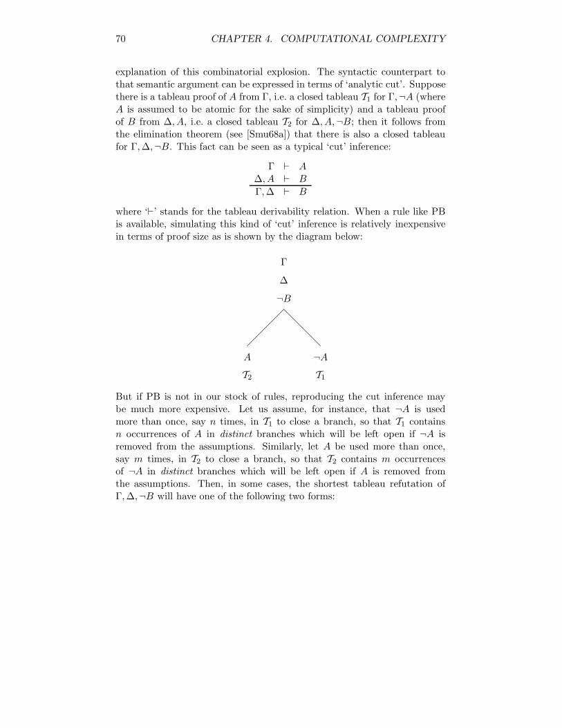
70 CHAPTER 4. COMPUTATIONAL COMPLEXITY
explanation of this combinatorial explosion. The syntactic counterpart tothat semantic argument can be expressed in terms of ‘analytic cut’. Supposethere is a tableau proof of A from Γ, i.e. a closed tableau T1 for Γ,¬A (whereA is assumed to be atomic for the sake of simplicity) and a tableau proofof B from ∆, A, i.e. a closed tableau T2 for ∆, A,¬B; then it follows fromthe elimination theorem (see [Smu68a]) that there is also a closed tableaufor Γ,∆,¬B. This fact can be seen as a typical ‘cut’ inference:
Γ ⊢ A∆, A ⊢ B
Γ,∆ ⊢ B
where ‘⊢’ stands for the tableau derivability relation. When a rule like PBis available, simulating this kind of ‘cut’ inference is relatively inexpensivein terms of proof size as is shown by the diagram below:
Γ
∆
¬B
��
��
@@
@@
A ¬A
T2 T1
But if PB is not in our stock of rules, reproducing the cut inference maybe much more expensive. Let us assume, for instance, that ¬A is usedmore than once, say n times, in T1 to close a branch, so that T1 containsn occurrences of A in distinct branches which will be left open if ¬A isremoved from the assumptions. Similarly, let A be used more than once,say m times, in T2 to close a branch, so that T2 contains m occurrencesof ¬A in distinct branches which will be left open if A is removed fromthe assumptions. Then, in some cases, the shortest tableau refutation ofΓ,∆,¬B will have one of the following two forms:
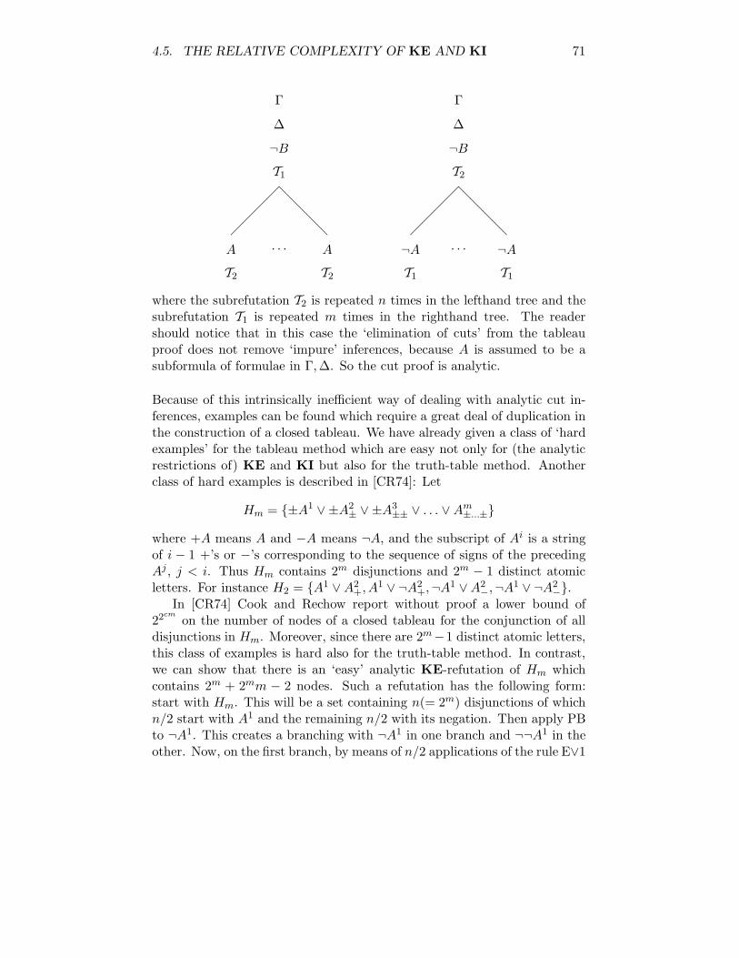
4.5. THE RELATIVE COMPLEXITY OF KE AND KI 71
Γ
∆
¬B
T1
��
��
@@
@@
· · ·A A
T2 T2
Γ
∆
¬B
T2
��
��
@@
@@
· · ·¬A ¬A
T1 T1
where the subrefutation T2 is repeated n times in the lefthand tree and thesubrefutation T1 is repeated m times in the righthand tree. The readershould notice that in this case the ‘elimination of cuts’ from the tableauproof does not remove ‘impure’ inferences, because A is assumed to be asubformula of formulae in Γ,∆. So the cut proof is analytic.
Because of this intrinsically inefficient way of dealing with analytic cut in-ferences, examples can be found which require a great deal of duplication inthe construction of a closed tableau. We have already given a class of ‘hardexamples’ for the tableau method which are easy not only for (the analyticrestrictions of) KE and KI but also for the truth-table method. Anotherclass of hard examples is described in [CR74]: Let
Hm = {±A1 ∨ ±A2± ∨ ±A3
±± ∨ . . . ∨ Am±...±}
where +A means A and −A means ¬A, and the subscript of Ai is a stringof i − 1 +’s or −’s corresponding to the sequence of signs of the precedingAj , j < i. Thus Hm contains 2m disjunctions and 2m − 1 distinct atomicletters. For instance H2 = {A1 ∨ A2
+, A1 ∨ ¬A2+,¬A1 ∨ A2
−,¬A1 ∨ ¬A2−}.
In [CR74] Cook and Rechow report without proof a lower bound of22cm
on the number of nodes of a closed tableau for the conjunction of alldisjunctions in Hm. Moreover, since there are 2m−1 distinct atomic letters,this class of examples is hard also for the truth-table method. In contrast,we can show that there is an ‘easy’ analytic KE-refutation of Hm whichcontains 2m + 2mm − 2 nodes. Such a refutation has the following form:start with Hm. This will be a set containing n(= 2m) disjunctions of whichn/2 start with A1 and the remaining n/2 with its negation. Then apply PBto ¬A1. This creates a branching with ¬A1 in one branch and ¬¬A1 in theother. Now, on the first branch, by means of n/2 applications of the rule E∨1
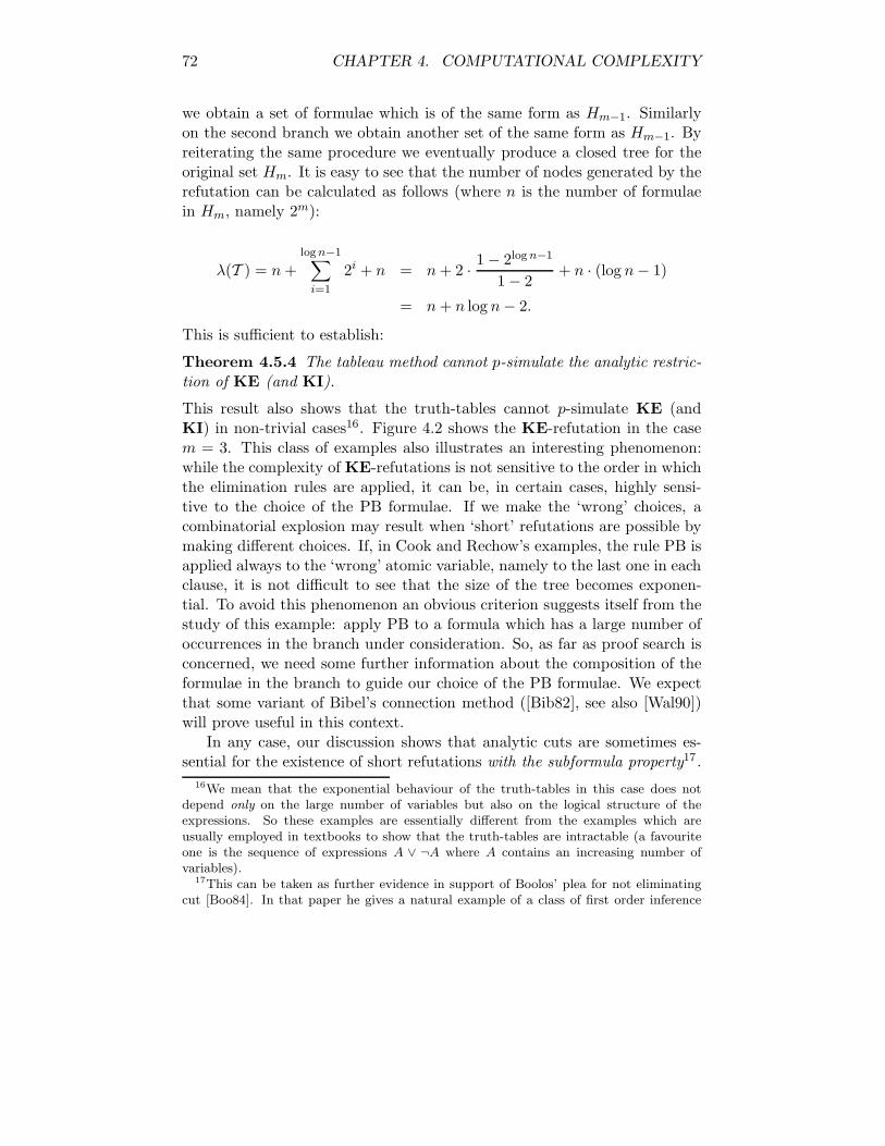
72 CHAPTER 4. COMPUTATIONAL COMPLEXITY
we obtain a set of formulae which is of the same form as Hm−1. Similarlyon the second branch we obtain another set of the same form as Hm−1. Byreiterating the same procedure we eventually produce a closed tree for theoriginal set Hm. It is easy to see that the number of nodes generated by therefutation can be calculated as follows (where n is the number of formulaein Hm, namely 2m):
λ(T ) = n +log n−1∑
i=1
2i + n = n + 2 ·1 − 2log n−1
1 − 2+ n · (log n − 1)
= n + n log n − 2.
This is sufficient to establish:
Theorem 4.5.4 The tableau method cannot p-simulate the analytic restric-tion of KE (and KI).
This result also shows that the truth-tables cannot p-simulate KE (andKI) in non-trivial cases16. Figure 4.2 shows the KE-refutation in the casem = 3. This class of examples also illustrates an interesting phenomenon:while the complexity of KE-refutations is not sensitive to the order in whichthe elimination rules are applied, it can be, in certain cases, highly sensi-tive to the choice of the PB formulae. If we make the ‘wrong’ choices, acombinatorial explosion may result when ‘short’ refutations are possible bymaking different choices. If, in Cook and Rechow’s examples, the rule PB isapplied always to the ‘wrong’ atomic variable, namely to the last one in eachclause, it is not difficult to see that the size of the tree becomes exponen-tial. To avoid this phenomenon an obvious criterion suggests itself from thestudy of this example: apply PB to a formula which has a large number ofoccurrences in the branch under consideration. So, as far as proof search isconcerned, we need some further information about the composition of theformulae in the branch to guide our choice of the PB formulae. We expectthat some variant of Bibel’s connection method ([Bib82], see also [Wal90])will prove useful in this context.
In any case, our discussion shows that analytic cuts are sometimes es-sential for the existence of short refutations with the subformula property17 .
16We mean that the exponential behaviour of the truth-tables in this case does notdepend only on the large number of variables but also on the logical structure of theexpressions. So these examples are essentially different from the examples which areusually employed in textbooks to show that the truth-tables are intractable (a favouriteone is the sequence of expressions A ∨ ¬A where A contains an increasing number ofvariables).
17This can be taken as further evidence in support of Boolos’ plea for not eliminatingcut [Boo84]. In that paper he gives a natural example of a class of first order inference

4.5. THE RELATIVE COMPLEXITY OF KE AND KI 73
H3
A1−
A2− ∨ A3
−+
A2− ∨ ¬A3
−+
¬A2− ∨ A3
−−
¬A2− ∨ ¬A3
−−
A2−
A3−+
¬A3−+
×
��� T
TT¬A2
−
A3−−
¬A3−−
×
,,, l
ll
¬A1
A2+ ∨ A3
++
A2+ ∨ ¬A3
++
¬A2+ ∨ A3
+−
¬A2+ ∨ ¬A3
+−
A2+
A3+−
¬A3+−
×
��� T
TT¬A2
+
A3++
¬A3++
×
Figure 4.2: A KE-refutation of H3.

74 CHAPTER 4. COMPUTATIONAL COMPLEXITY
4.5.3 KE versus Natural Deduction
It can also be shown that KE can linearly simulate natural deduction (intree form). Moreover the simulation procedure preserves the subformulaproperty. We shall sketch this procedure for the natural deduction systemgiven in [Pra65], the procedure being similar for other formulations.
We want to give an effective proof of the following theorem (where NDstands for Natural Deduction):
Theorem 4.5.5 If there is an ND-proof T of A from Γ, then there is aKE-proof T ′ of A from Γ such that λ(T ′) ≤ 3λ(T ) and T ′ contains onlyformulae A such that A occurs in T .
Proof. By induction on λ(T ).If λ(T ) = 1, then the ND-tree consists of only one node which is an as-sumption, say C. The corresponding KE-tree is the closed sequence C,¬C.If λ(T ) = k, with k > 1, then there are several cases depending on whichrule has been applied in the last inference of T . We shall consider only thecases in which the rule is elimination of conjunction (E∧) and elimination ofdisjunction (E∨), and leave the others to the reader. If the last rule appliedin T is E∧, then T has the form:
T =
∆T1
A ∧ B
A
By inductive hypothesis there is a KE-refutation T ′1 of ∆,¬(A ∧ B) such
that λ(T ′1 ) ≤ 3λ(T1). Then the following KE-tree:
schemata which are ‘hard’ for the tableau method while admitting of ‘easy’ (non-analytic)natural deduction proofs. Boolos’ example is a particularly clear illustration of the well-known fact that the elimination of cuts from proofs in a system in which cuts are eliminablecan greatly increase the complexity of proofs. (For a related technical result see [Sta78].)KE and KI provide an elegant solution to Boolos’ problem by making cut non-eliminablewhile preserving the subformula property of proofs. Our discussion also shows that elim-inating analytic cuts can result in a combinatorial explosion.

4.5. THE RELATIVE COMPLEXITY OF KE AND KI 75
T ′ =
∆
¬A
��
��
@@
@@
A ∧ B ¬(A ∧ B)
T ′1A
×
is the required KE-proof and it is easy to verify that λ(T ′) ≤ 3λ(T ).
If the last rule applied in T is the rule of elimination of disjunction, then Thas the form:
T =
∆1 ∆2, [A] ∆3, [B]T1 T2 T3
A ∨ B C C
C
By inductive hypothesis there are KE-refutations T ′1 of ∆1,¬(A∨B), T ′
2 of∆2, A,¬C, and T ′
3 of ∆3, B,¬C, such that λ(T ′i ) ≤ 3λ(Ti), i = 1, 2, 3. Then
the following KE-tree:
T ′ =
∆1
∆2
∆3
¬C
��
��
@@
@@
A ∨ B ¬(A ∨ B)
T ′1�
��
�
@@
@@
A ¬A
T ′2 B
T ′3

76 CHAPTER 4. COMPUTATIONAL COMPLEXITY
Structural rules
∆[Thin]
∆, A
∆, A, B, Λ[Perm]
∆, B, A, Λ
∆, A, A[Cont]
∆, A
Logical rules
∆, A Λ, B[∧I]
∆, Λ, A ∧ B
∆, A ∧ B[∧E-1]
∆, A
∆, A ∧ B[∧E-2]
∆, B
∆, A,B[∨I]
∆, A ∨ B
∆, A ∨ B[∨E]
∆, A,B
[A]∆, B
[→I]∆, A → B
∆, A Λ, A → B[→E]
∆, Λ, B
[A]∆
[¬I]∆,¬A
∆, A Λ,¬A[¬E]
∆, Λ
Table 4.1: A sequent-conclusion natural deduction system.
is the required proof and it is easy to verify that λ(T ′) ≤ 3λ(T ).2
In [Cel88] Cellucci has proposed a new form of natural deduction whichhe has shown in several examples to produce shorter proofs than Prawitz’sstyle natural deduction. In Cellucci’s system, as in natural deduction, as-sumptions are introduced which may subsequently be discharged; howeverthe inference rules involve sequents rather than single formulae. The rulesof the propositional fragment are shown in table 4.1. (∆ and Λ representssequences of formulae, not sets. If they are taken to represent sets, the rulesPerm and Cont become redundant.)
According to Cellucci, derivations in his system are ‘significantly simpler(i.e. contain fewer symbols) than in [Prawitz’s style] system’18. It is notdifficult to show, by means of an argument analogous to the one given above
18[Cel88, p.29].

4.6. A MORE GENERAL VIEW 77
for Prawitz’s style natural deduction, that:
Theorem 4.5.6 If there is a proof π in Cellucci’s system of the sequent ∆from assumptions Γ, then there is a KE-refutation π′ of Γ,∆, where ∆ isequal to {¬B | B ∈ ∆}, such that λ(π′) ≤ 3λ(π). Moreover, the simulationpreserves the subformula property.
4.5.4 KE and resolution
The relationship between KE and resolution-like methods has been dis-cussed in Section 3.4. We can easily adapt the KE-rules to deal with for-mulae in clausal form and, once this has been done, the system is seen toincorporate the basic idea underlying resolution theorem proving as a specialcase. As far as the relative complexity of KE and resolution is concerned,within the domain of clausal form logic, it depends on how refutations arerepresented. If propositional resolution is represented as in [DLL62], i.e. asa combination of unit resolution and the splitting rule, its complexity is thesame as that of the clausal form fragment of KE. This way of representingresolution is much clearer and appears to be more convenient from a prac-tical point of view, in that it seems to reduce the generation of redundantclauses. If the resolution rule is defined in the more usual way as a singlerule, and refutations are represented as sequences or directed acyclic graphsof clauses, it is easy to see that KE can linearly simulate resolution witha procedure which involves only subformulae of the formulae occurring inthe given resolution refutation. Such a refutation will be, strictly speaking,non-analytic because the resolution rule does not have the subformula prop-erty. An open question is whether or not the analytic restriction of KE canefficiently simulate the standard version of resolution. We conjecture thatit can19.
4.6 A more general view
As seen in section 4.5.2, the speed-up of KE over the tableau method can betraced to the fact that KE, unlike the tableau method, can easily simulateinference steps based on ‘cuts’, like the example on p.70. In other words,KE allows a uniform method for grafting proofs of subsidiary conclusions,or lemmata, in the proof of a theorem. However, the existence of such a uni-form method is by no means sufficient. In Natural Deduction, for instance,replacing every occurrence of an assumption A with its proof provides an
19If resolution refutations are represented in tree form, it is not difficult to see that sucha simulation is possible.

78 CHAPTER 4. COMPUTATIONAL COMPLEXITY
obvious grafting method which, though very perspicuous, is highly ineffi-cient, leading to much unwanted duplication in the resulting proof-tree. Weshould then require that the method be also efficient. A way of making thisrequirement precise is to ask that the following condition be satisfied by aproof system S:
(C) Let π1 be a proof of A from Γ and let π2 be a proof of B from ∆, A, thenthere is a uniform method for constructing from π1 and π2 a proof π3
of B from Γ,∆ such that λ(π3) ≤ λ(π1) + λ(π2) + c for some constantc.
It can be easily seen that condition (C) is satisfied by KE and KI, therequired method being the one described on p.70. In contrast, the standardway of grafting proofs of subsidiary conclusions in Natural Deduction proofs,though providing a uniform method, does not satisfy the further conditionon the complexity of the resulting proof. The rules of Natural Deduction,however, permit us to bypass this difficulty and produce a method satisfyingthe whole of condition (C). Consider the rule of Non-Constructive Dilemma(NCD):
Γ, [A] ∆, [¬A]...
...B B
B
This is a derived rule in Prawitz’s style Natural Deduction which yieldsclassical logic if added to the intuitionistically valid rules (see [Ten78, section4.5]). We can show Natural Deduction to satisfy condition (C) by means ofthe following construction:
∆...
Γ, [A] A [¬A]... FB B
B
Notice that the construction does not depend on the number of occurrencesof the assumption A in the subproof of B from Γ, A.
In analogy to condition (C) we can formulate a condition requiring aproof system to simulate efficiently another form of cut which holds forclassical systems and is closely related to the rule PB:

4.6. A MORE GENERAL VIEW 79
(C*) Let π1 be a proof of B from Γ, A and π2 be a proof of B from ∆,¬A.Then there is a uniform method for constructing from π1 and π2 aproof π3 of B from Γ,∆ such that λ(π3) ≤ λ(π1) + λ(π2) + c for someconstant c.
Similarly, the next condition requires that proof systems can efficiently sim-ulate the ex falso inference scheme:
(XF) Let π1 be a proof of A from Γ and π2 be a proof of ¬A from ∆. Thenthere is a uniform method for constructing from π1 and π2 a proof π3
of B from Γ,∆, for any B, such that λ(π3) ≤ λ(π1) + λ(π2) + c forsome constant c.
So, let us say that a classical proof system is a classical cut system if itsatisfies conditions (C*) and (XF). It is easy to show that every classical cutsystem satisfies also condition (C) above and, therefore, allows for an efficientimplementation of the transitivity property of natural proofs. The nexttheorem shows that every classical cut system can simulate KE without asignificant increase in proof complexity and with a procedure which preservesthe subformula property20. This clearly shows that it is only the use of(analytic) cut and not the form of the operational rules which is crucialfrom a complexity viewpoint (this will be further discussed in chapter 6).
Theorem 4.6.1 If S is a classical cut system, then S can linearly simulateKE (and KI) with a procedure which preserves the subformula property.
To prove the theorem it is convenient to assume that our language includesa 0-ary operator F (Falsum) and that the proof systems include suitablerules to deal with it21. For KE this involves only adding the obvious rulewhich allows us to append F to any branch containing both A and ¬A forsome formula A, so that every closed branch in a KE-tree ends with a nodelabelled with F . The assumption is made only for convenience’s sake andcan be dropped without consequence. Moreover we shall make the obviousassumption that, for every system S, the complexity of a proof of A from Ain S is equal to 1.
Let τ(π) denote the number of nodes generated by a KE-refutation π ofΓ (i.e. the assumptions are not counted)22. Let S be a classical cut system.
20In this chapter we are restricting ourselves to analytic proof systems, i.e. proof systemswhich enjoy the subformula property.
21Systems which are not already defined over a language containing F can usually beredefined over such an extended language without difficulty.
22The reader should be aware that our τ -measure applies to KE-refutations and not
to trees: the same tree can represent different refutations yielding different values of theτ -measure.

80 CHAPTER 4. COMPUTATIONAL COMPLEXITY
If S is complete, then for every rule r of KE there is an S-proof πr of theconclusion of r from its premises. Let b1 = Maxr(λ(πr)) and let b2 and b3 bethe constants representing, respectively, the λ-cost of simulating classical cutin S — associated with condition (C*) above — and the λ-cost of simulatingthe ex falso inference scheme in S — associated with condition (XF) above.As mentioned before, every classical cut system satisfies also condition (C)and it is easy to verify that the constant associated with this condition,representing the λ-cost of simulating ‘absolute’ cut in S, is ≤ b2 + b3 + 1.We set c = b1 + b2 + b3 + 1.
The theorem is an immediate consequence of the following Lemma:
Lemma 4.6.1 For every classical cut system S, if there is a KE-refutationπ of Γ, then there is an S-proof π′ of F from Γ with λ(π′) ≤ c · τ(π).
Proof. The proof is by induction on τ(π), where π is a KE-refutationof Γ.
τ(π) = 1. Then Γ is explicitly inconsistent, i.e. contains a pair of com-plementary formulae, say B and ¬B, and the only node generated by therefutation is F , which is obtained by means of an application of the KE-rulefor F to B and ¬B. Since there is an S-proof of the KE-rule for F , we canobtain an S-proof π′ of the particular application contained in π simply byperforming the suitable substitutions and λ(π′) ≤ b1 < c.
τ(π) > 1. Case 1. The KE-refutation π has the form:
Γ
C
T1
where C follows from premises in Γ by means of an E-rule. So there is a KE-refutation π1 of Γ, C such that τ(π) = τ(π1) + 1. By inductive hypothesis,there is an S-proof π′
1 of F from Γ, C such that λ(π′1) ≤ c · τ(π1). Moreover,
there is an S-proof π2 of C from the premises from which it is inferred inπ such that λ(π2) ≤ b1. So, from the hypothesis that S is a classical cutsystem, it follows that there is an S-proof π′ of F from Γ such that
λ(π′) ≤ c · τ(π1) + b1 + b2 + b3 + 1
≤ c · τ(π1) + c
≤ c · (τ(π1) + 1)
≤ c · τ(π)

4.6. A MORE GENERAL VIEW 81
Case 2. π has the following form:
Γ
��
��
@@
@@
C ¬C
T1 T2
So there are KE-refutations π1 and π2 of Γ, C and Γ,¬C respectively suchthat τ(π) = τ(π1) + τ(π2) + 2. Now, by inductive hypothesis there is anS-proof π′
1 of F from Γ, C and an S-proof π′2 of F from Γ,¬C with λ(π′
i) ≤c · τ(πi), i = 1, 2. Since S is a classical cut system, it follows that there is anS-proof π′ of F from Γ such that
λ(π′) ≤ c · τ(π1) + c · τ(π2) + b2
< c · τ(π1) + c · τ(π2) + c
< c · (τ(π1) + τ(π2) + 2)
< c · τ(π)
2
It follows from Theorem 4.6.1 and Theorem 4.5.2 that:
Corollary 4.6.1 Every analytic cut system is a standard proof system, i.e.for every tautology A of length n and containing k distinct variables there isa proof π, with λ(π) = O(n · 2k).
Moreover, Theorem 4.6.1, Theorem 4.5.3 and Theorem 4.5.4 imply that:
Corollary 4.6.2 Every analytic cut system can linearly simulate the tableaumethod, but the tableau method cannot p-simulate any analytic cut system.
Since (the classical version of) Prawitz’s style natural deduction is a classicalcut system, it follows that it can linearly simulate KE. The same holds alsofor Cellucci’s system and for the ‘natural deduction’ variant of KE describedin Section 3.8 under the name KEND. Moreover, for all these systems, thesimulation preserves the subformula property (i.e. it maps analytic proofs toanalytic proofs). Therefore Theorem 4.6.1, together with Theorems 4.5.1,4.5.5 and 4.5.6, imply that Prawitz’s style natural deduction, Cellucci’s nat-ural deduction, KE, KEND and KI can linearly simulate each other with

82 CHAPTER 4. COMPUTATIONAL COMPLEXITY
a procedure which preserves the subformula property. Corollary 4.2 im-plies that all these systems are essentially more efficient than the tableaumethod, even if we restrict our attention to analytic proofs (the tableaumethod cannot p-simulate any analytic cut system). Finally Corollary 4.6.1implies that, unlike the tableau method, all these systems are standard proofsystems, i.e. have the same upper bound as the truth-table method.
Chapter 5
Belnap’s four valued logic
5.1 Introduction
The study of first-degree entailment occupies a special position in the field ofrelevance logics: it can be seen either as the study of the validity of formulaeof the form A → B, where → is Anderson and Belnap’s relevant implicationand A, B are implication-free formulae, or as the study of the notion of rele-vant deducibility between standard formulae built-up from the usual connec-tives. In the latter interpretation it is associated with the problem — well-known to computer scientists who work in the area of Automated Deduction— of obtaining sound information from possibly inconsistent databases1. Aninteresting semantic characterization of first-degree entailment was given byBelnap in [Bel77] who also emphasized its connections with the problem of‘how a computer should think’[Bel76]. In [Dun76] Dunn presented a tableausystem based on a modification of Jeffrey’s method of ‘coupled trees’ [Jef81].In this chapter we study the consequence relation associated with Belnap’ssemantics and produce two different calculi which are sound and completefor it. Unlike Dunn’s ‘coupled tree’ calculus, our calculi use one tree only.This simplification allows us to exploit fully the formal analogy with thecorresponding classical calculi, and to obtain simple extensions to a firstorder version of Belnap’s logic (neither Jeffrey nor Dunn explain how themethod of ‘coupled trees’ can be extended to deal with quantifiers).
In sections 5.2 and 5.3 we briefly discuss the background problem andillustrate Belnap’s semantics. In section 5.4 we formulate a tableau methodwhich produces ‘single’ instead of ‘coupled’ tableaux, and prove it sound andcomplete for (the first-order version of) the consequence relation associated
1For recent contributions in this area and in the related one of logic programming, see[DCHLS90] and [BS89].
83
84 CHAPTER 5. BELNAP’S FOUR VALUED LOGIC
with Belnap’s semantics. Then, in section 5.5, we define another calculusbased on the classical systems KE which has been studied in Chapter 3.
5.2 ‘How a computer should think’
Deductive Reasoning is often described as a process of revealing ‘hidden’information from explicit data and, as such, it is a basic tool in the area of‘intelligent’ database management or question-answering systems. Unfortu-nately, the most time-honoured and well-developed framework for deductivereasoning — classical logic — is unsuitable to this purpose. The reasonis that databases, especially large ones, have a great propensity to becomeinconsistent : first, the information stored is usually obtained from differentsources which might conflict with each other; second, the information ob-tained from each source, even if it is not obviously inconsistent, may ‘hide’contradictions. But it is well-known that classical two-valued logic is over-sensitive to contradictions: if Γ is an inconsistent set of sentences, then— according to classical logic — any sentence follows from Γ. This doesnot imply, of course, that classical logic is incorrect, but only suggests thatthere are circumstances in which it is highly recommendable to abandon itand use another. A radical solution to this problem would be to requireany database to be consistent before starting deductive processing. But, forpractical reasons, this ‘solution’ is no better than the original problem: first,contradictions do not always lie on the surface, and the only way to detectsuch implicit contradictions is to apply deductive reasoning itself; second,even explicit contradictions may not be removable because they originatein conflicting data fed into the computer by different and equally reliablesources.
But if classical logic is not to be recommended for application in de-ductive database management, what kind of logic is the one with which acomputer should ‘think’?
5.3 Belnap’s four-valued model
In this chapter we shall make use of the approach developed by Belnap[Bel77, Bel76] on the basis of a work of Dunn [Dun76]. Let 4 denote the set{T, F, Both, None}. The elements of 4 are called truth-values. Belnapcalls them ‘told values’ to emphasize their epistemic character. We maythink of them as the four possible ways in which an atomic sentence P canbelong to the ‘present state of information’ : (1) the computer is told thatP is true (and is not told that P is false); (2) the computer is told that P

5.3. BELNAP’S FOUR-VALUED MODEL 85
is false (and is not told that P is true); (3) the computer is told that P isboth true and false (perhaps from different sources, or in different instantsof time); (4) the computer is not told anything about the truth value of P .
The values of complex sentences are obtained by Belnap by means ofmonotony considerations, based on Scott’s approximation lattices, resultingin the following tables:
None F T Both
¬ None T F Both
∧ None F T Both
None None F None F
F F F F F
T None F T Both
Both F F Both Both
∨ None F T Both
None None None T T
F None F T Both
T T T T T
Both T Both T Both
These tables represent a lattice which is called L4:
F
@@
@@
None ��
��
T
@@
@@ Both�
��
�
We define a set-up as a mapping of atomic formulae into 4. Using the
86 CHAPTER 5. BELNAP’S FOUR VALUED LOGIC
truth-tables given above, every set-up can be extended to a mapping of allformulae into 4 in the usual inductive way. We shall call such an extendedmapping a 4-valuation .
Definition 5.3.1 We say that A entails B, and write A → B, if for all 4-valuations v, v(A) � v(B), where � is the partial ordering associated withthe lattice L4. We also say that a non empty set of formulae Γ entails A,and write Γ ⊢ A, if the conjunction of all formulae in Γ entails A.
Notice that the relation ⊢ mentioned in Def. 5.3.1 is a monotonic conse-quence relation.
The logic characterized by Belnap’s semantics corresponds to the logic offirst-degree entailment (see [AB75, section 15.2]). This system admits ofthe following Hilbert-style formulation:
Axioms:
A ∧ B → A(5.1)
A ∧ B → B(5.2)
A → A ∨ B(5.3)
B → A ∨ B(5.4)
A ∧ (C ∨ B) → (A ∧ B) ∨ C(5.5)
A → ¬¬A(5.6)
¬¬A → A(5.7)
Rules:
A → B,B → C ⊢ A → C(5.8)
A → B,A → C ⊢ A → B ∧ C(5.9)
A → C,B → C ⊢ A ∨ B → C(5.10)
A → B ⊢ ¬B → ¬A(5.11)
Let us now introduce some useful terminology:
Definition 5.3.2 Let us say, given a 4-valuation v, that a formula A is:
1. at least true under v if v(A) = T or v(A) = Both.
2. non-true under v if v(A) = F or v(A) = None.
3. at least false under v if v(A) = F or v(A) = Both.
5.4. SEMANTIC TABLEAUX FOR BELNAP’S LOGIC 87
4. non-false under v if v(A) = T or v(A) = None.
It is not difficult to see that the definition of Γ ⊢ A given in Definition 5.3.1is equivalent to the following one:
Definition 5.3.3 Γ ⊢ A if and only if for every 4-valuation v, (i) if all theelements of Γ are at least true under v, then A is at least true under v and(ii) if all the elements of Γ are non-false under v, then A is non-false underv.
5.4 Semantic tableaux for Belnap’s logic
In this section we suggest a tableau method which, unlike Dunn’s one, usesonly one tree. The resulting tableaux are binary trees and are identical toclassical tableaux of signed formulae except that they contain four types ofs-formulae instead of two.
5.4.1 Propositional tableaux
Signed Formulae. We introduce the symbols t, f, t∗, f∗ and define a signedformula as an expression of the form t(A), f(A), t∗(A) or f∗(A), where A isan unsigned formula. Intuitively we interpret ‘t(A)’ as ‘A is at least true’,‘f(A)’ as ‘A is non-true’, ‘t∗(A)’ as ‘A is non-false’ and ‘f∗(A)’ as ‘A is atleast false’.
The conjugate of an s-formula s(A) is:
f(A) if s = tt(A) if s = ff∗(A) if s = t∗
t∗(A) if s = f∗
The converse of an s-formula s(A) is:
t∗(A) if s = tt(A) if s = t∗
f∗(A) if s = ff(A) if s = f∗
We are now in a position to formulate our tableau rules which are given inTable 5.1. The reader will notice the formal analogy with the classical rules.

88 CHAPTER 5. BELNAP’S FOUR VALUED LOGIC
t(A ∧ B)
t(A)t(B)
t∗(A ∧ B)
t∗(A)t∗(B)
f(A ∨ B)
f(A)f(B)
f∗(A ∨ B)
f∗(A)f∗(B)
f(A ∧ B)
f(A) f(B)
f∗(A ∧ B)
f∗(A) f∗(B)
t(A ∨ B)
t(A) t(B)
t∗(A ∨ B)
t∗(A) t∗(B)
t(¬A)
f∗(A)
t∗(¬A)
f(A)
f(¬A)
t∗(A)
f∗(¬A)
t(A)
Table 5.1: Propositional tableau rules for Belnap’s four valued logic.
α α1 α2
t(A ∧ B) t(A) t(B)
t∗(A ∧ B) t∗(A) t∗(B)
f(A ∨ B) f(A) f(B)
f∗(A ∨ B) f∗(A) f∗(B)
t(¬A) f∗(A) f∗(A)
t∗(¬A) f(A) f(A)
f(¬A) t∗(A) t∗(A)
f∗(¬A) t(A) t(A)
Table 5.2: Formulae of type α.
It may be useful to extend Smullyan’s unifying notation to cover the newtypes of s-formulae which occur in our language.
We use the letter ‘α’ to stand for any s-formula of one of the forms:t(A∧B), t∗(A∧B), f(A∨B), f∗(A∨B), t(¬A), t∗(¬A), f(¬A) and f∗(¬A). Forevery such formula α, its components α1 and α2 are defined as in Table 5.2.We use ‘β’ to stand for any formula of one of the forms: f(A∧B), f∗(A∧B),t(A ∨ B) or t∗(A ∨B). For every such formula β, its components β1 and β2
are defined as in the Table 5.3. So our tableau rules can be ‘packed’ intothe following two rules:
Rule A
α
α1
α2
Rule Bβ
β1 β2
We say that a branch φ of a tableau is closed if it contains both an s-formula and its conjugate. Otherwise we say that φ is open. A tableau isclosed if all its branches are closed. Otherwise it is open. A formula A isprovable from the set of formulae Γ if and only if there is a closed tableau

5.4. SEMANTIC TABLEAUX FOR BELNAP’S LOGIC 89
β β1 β2
f(A ∧ B) f(A) f(B)
f∗(A ∧ B) f∗(A) f∗(B)
t(A ∨ B) t(A) t(B)
t∗(A ∨ B) t∗(A) t∗(B)
Table 5.3: Formulae of type β.
for {t(B)|B ∈ Γ} ∪ {f(A)}.
An example of a closed tableau representing a proof of ((A ∨ B) ∧ ¬A) →(B∨(A∧¬A)) is given in Fig. 5.1. A failed attempt at proving the disjunctivesyllogism is shown in Fig. 5.2.
Soundness.
Definition 5.4.1 Let us say that a 4-valuation v realizes s(A) if
1. s(A) = t(A) and A is at least true under v.
2. s(A) = f(A) and A is non-true under v.
3. s(A) = t∗(A) and A is non-false under v
4. s(A) = f∗(A) and A is at least false under v.
A set U of s-formulae is said to be realizable if there is a 4-valuation v whichrealizes every element of U .
In order to prove soundness we need the following lemma:
Lemma 5.4.1 If T is a closed tableau for U , where U is a set of signedformulae, then the tableau T ′ obtained from T by replacing every (occurrenceof an) s-formula with (an occurrence of) its converse is a closed tableau forthe set U∗ of the converses of the s-formulae in U .
The proof is a straightforward induction on the number of nodes in a closedtableau.
Now, it is easy to verify that our tableau rules are correct in the sense thatevery 4-valuation which realizes the premise of the rule A realizes also boththe conclusions of the rule, and every 4-valuation which realizes the premise

90 CHAPTER 5. BELNAP’S FOUR VALUED LOGIC
t(A) t(B) t∗(A)
��
��
@@
@@
f(A) f(¬A)
��
��
@@
@@
f(A ∧ ¬A)
f(B)
f∗(A)
t(¬A)
t(A ∨ B)
f(B ∨ (A ∧ ¬A))
t((A ∨ B) ∧ ¬A)
Figure 5.1: A proof of ((A ∨ B) ∧ ¬A) → (B ∨ (A ∧ ¬A))

5.4. SEMANTIC TABLEAUX FOR BELNAP’S LOGIC 91
t(A) t(B)
��
��
@@
@@
f∗(A)
t(¬A)
t(A ∨ B)
f(B)
t((A ∨ B) ∧ ¬A)
Figure 5.2: A failed attempt to prove the disjunctive syllogism
of the rule B realizes also at least one of the conclusions of the rule. Thereforeit follows, by an elementary inductive argument, that if a 4-valuation vrealizes all the initial s-formulae of a tableau T , then there is at least onebranch φ of T such that v realizes all the s-formulae occurring in φ. But, ofcourse, no 4-valuation can realize two conjugate s-formulae simultaneously.Therefore if T is a a closed tableau, no 4-valuation can realize all the initials-formulae of T . So, if T is a closed tableau for {t(B)|B ∈ Γ} ∪ {f(A)},it follows that for every 4-valuation v, A is at least true in v whenever allformulae in Γ are. Moreover it follows from lemma 5.4.1 that no 4-valuationcan realize the converses of all the initial signed formulae of T , i.e. no 4-valuation can realize {t∗(B)|B ∈ Γ} ∪ {f∗(A)}. Hence for every 4-valuationv, A is non-false in v whenever all the formulae in Γ are. So, by def. 5.3.3,Γ ⊢ A. This concludes the proof.
Completeness. Let us say that a branch φ of a tableau T is complete if (i)for every α in φ both α1 and α2 occur in φ and (ii) for every β in φ at leastone of β1, β2 occurs in φ. Let us also say that a tableau T is completed whenevery branch of T is complete. We have the following theorem:
Theorem 5.4.1 Every complete open branch of any tableau is realizable.
We shall first define the analog of Hintikka sets within our framework. Thetheorem will then immediately follow from the analog of Hintikka’s lemma.

92 CHAPTER 5. BELNAP’S FOUR VALUED LOGIC
Definition 5.4.2 Let us say that a set of signed formulae U is an R-Hintikkaset if and only if it satisfies the following conditions:
H0: No signed variable and its conjugate are both in U .
H1: If α ∈ U , then α1 ∈ U and α2 ∈ U .
H2: If β ∈ U , then β1 ∈ U or β2 ∈ U .
It follows from our definitions that the set of s-formulae in a complete openbranch of any tableau is an R-Hintikka set. Then the theorem is an imme-diate consequence of the following lemma:
Lemma 5.4.2 Every R-Hintikka set is realizable.
Proof. Let U be an R-Hintikkka set. Let us assign to each variable P whichoccurs in at least an element of U a value in 4 as follows:
(1) If t(P ) ∈ U , and f∗(P ) 6∈ U , give P the value T.(2) If t(P ) ∈ U , and f∗(P ) ∈ U , give P the value Both.(3) If f(P ) ∈ U , and t∗(P ) 6∈ U , give P the value F.(4) If f(P ) ∈ U , and t∗(P ) ∈ U , give P the value None.(5) if t∗(P ) ∈ U , and f(P ) 6∈ U , give P the value T.(6) if f∗(P ) ∈ U , and t(P ) 6∈ U , give P the value F.
Now it is obvious that the 4-valuation induced by this assignment realizesall the signed variables occurring in U . Then we only need to observe that
(i) If a 4-valuation realizes both α1 and α2, then it realizes also α.
(ii) If a 4-valuation realizes at least one of β1,β2 then it realizes also β.
The lemma then follows from an easy induction on the complexity of thes-formulae in U .
Theorem 5.4.1 implies
Theorem 5.4.2 (Completeness Theorem) If Γ ⊢ A then there is a closedtableau for {t(B)|B ∈ Γ} ∪ {f(A)}.
5.4.2 Detecting inconsistencies
Although we do not want inconsistencies to have the catastrophic effect thatthey have in classical logic, it would be desirable to be able to check our

5.4. SEMANTIC TABLEAUX FOR BELNAP’S LOGIC 93
databases for consistency. After all, we do not want to ‘glorify’ contradic-tions. On the contrary we usually want to remove them.
Fortunately, consistency checks are quite easy to carry out without mod-ifying our framework. We shall show that, in fact, our tableaux ‘contain’their classical version: to obtain classical tableaux we only need to modifythe closure condition on a branch.
Definition 5.4.3 The weak conjugate of an s-formula is defined as in thefollowing table:
Signed formula Weak conjugate
t(A) f∗(A)f(A) t∗(A)t∗(A) f(A)f∗(A) t(A)
We say that a branch φ of a tableau T is weakly closed if φ contains ans-formula and its weak conjugate. The tableau T is weakly closed if all itsbranches are weakly closed.
Let us use s as a variable ranging over signs, i.e. over the symbols {t, f, t∗, f∗}.By s we mean:
f if s = tt if s = ff∗ if s = t∗
t∗ if s = f∗
By s∗ se mean:
t∗ if s = tf∗ if s = ft if s = t∗
f if s = f∗
We have the following lemma:
Lemma 5.4.3 Let us say that a set of s-formulae S is homogeneous if allthe s-formulae in it have the same sign s. Then if S is a homogeneous setof s-formulae, every tableau T for S contains only s-formulae with sign s ors∗.
Proof: By inspection of the rules and induction on the rank of the s-formulae occurring in T .

94 CHAPTER 5. BELNAP’S FOUR VALUED LOGIC
The following theorem states the connection between classical and relevantderivability:
Theorem 5.4.3 Γ is a (classically) unsatisfiable set of formulae if and onlyif there is a weakly closed tableau for {t(B)|B ∈ Γ}. Therefore A is clas-sically deducible from Γ if and only if there is a weakly closed tableau for{t(B)|B ∈ Γ} ∪ {t(¬A)}.
Proof: If Γ is classically unsatisfiable, there is a closed classical tableaufor {t(B)|B ∈ Γ}. It is easy to see that the tableau obtained from it byreplacing each sign f with f∗ is a weakly closed tableau for {t(B)|B ∈ Γ}.
Suppose there is a weakly-closed tableau T for {t(B)|B ∈ Γ}. ByLemma 5.4.3 this tableau can contain only formulae signed with t or f∗.Therefore every weakly-closed branch contains t(A) and f∗(A) for some A.It follows that every 4-valuation which realizes the initial formulae, mustrealize both t(A) and f∗(A) for some A, i.e. it must assign Both to A forsome A. Hence there is no boolean valuation which satisfies Γ.
As we said before, the notion of weakly closed tableau is useful in that aweakly closed tableau shows an inconsistency in our database and, there-fore, the need for revision. So our tableaux are sensitive to contradictionslike classical tableaux; unlike classical tableaux, however, when they detecta contradiction they do not panic but keep on making ‘sensible’ deductions.
We observe that, in our approach, an initial formula of the form f(A)always represents a ‘query’, whereas data are represented by initial formulaeof the form t(A). So, checking our data for consistency and answeringquestions on the base of our data are formally distinct tasks.
5.4.3 First-order tableaux
Another advantage of our single-tableau formulation is in the treatment ofquantifiers. These are dealt with by means of rules obtained, as in thecase of the binary connective rules, by taking over the standard classicalrules (for s-formulae) and supplementing them with their ‘starred’ versions.By contrast, the suitable quantifier rules for the first-order version of themethod of coupled-trees are not so straightforward.
We consider a standard first-order language with no functional symbols.We use the letters x, y, z, . . . (possibly with subscripts) as individual variablesand the letters a, b, c, . . . (possibly with subscripts) as parameters. For anyvariable x and parameter a, A(x/a) will be the result of substituting all thefree occurrences of x in A with a. Subformulae are defined in the usual way,so that for every parameter a, A(x/a) is a subformula of ∀xA(x).

5.4. SEMANTIC TABLEAUX FOR BELNAP’S LOGIC 95
An obvious way of extending Belnap’s semantics to formulae containingquantifiers is the following:
Let U be a non-empty universe. We assume a set U of constants namingthe elements of U (of course neither U nor U need to be denumerable).By a U -formula we mean a formula built up from the logical operators, therelation symbols, the individual variables and the constants in U . (Thusa U -formula is like a formula with parameters but with elements of U inplace of parameters.) Let FU be the set of closed U -formulae. A first-ordervaluation over U is defined as a mapping v of all elements of FU into 4 suchthat (i) v is a 4-valuation (see above p. 86) and (ii) v satisfies the followingadditional conditions for quantifiers (where ⊓V and ⊔V denote, respectively,the g.l.b. and the l.u.b. of the set V in L4):
v(∀x(A(x)) = ⊓{v(A(k/x))|k ∈ U}
v(∃x(A(x)) = ⊔{v(A(k/x))|k ∈ U}
The first-order consequence relation associated with this extended semanticsis then:
Definition 5.4.4 Γ ⊢ A if and only if for every universe U and all first-order valuations v over U, (i) if all elements of Γ are at least true under v,then A is at least true under v and (ii) if all the elements of Γ are non-falseunder v, then A is non-false under v.
The quantifier rules are the expected ones:
t(∀xA(x))
t(A(a/x))for all a
t∗(∀xA(x))
t∗(A(a/x))
f(∀xA(x))
f(A(a/x))with a new
f∗(∀xA(x))
f∗(A(a/x))
t(∃xA(x))
t(A(a/x))with a new
t∗(∃xA(x))
t∗(A(a/x))
f(∃xA(x))
f(A(a/x))for all a
f∗(∃xA(x))
f∗(A(a/x))
It is convenient to use Smullyan’s notation for quantified formulae. So γwill denote any formula of one of the four forms t(∀xA(x)), t∗(∀xA(x)),f(∃xA(x)), f∗(∃xA(x)) and by γ(a) we shall mean, respectively, t(A(x/a)),t∗(A(x/a)), f(A(x/a)), f∗(A(x/a)). Similarly δ will denote any formula ofone of the four forms t(∃xA(x)), t∗(∃xA(x)), f(∀xA(x)), f∗(∀xA(x)) and

96 CHAPTER 5. BELNAP’S FOUR VALUED LOGIC
and by δ(a) we shall mean, respectively, t(A(x/a)), t∗(A(x/a)), f(A(x/a)),f∗(A(x/a)).
Thus, our first-order rules can be succintly expressed by the followingtwo rules:
Rule Cγ
γ(a) for any parameter a
Rule Dδ
δ(a) for a new parameter a
Soundness and completeness of this first-order system can be proved —given the corresponding proofs for the propositional fragment — by meansof straightforward adaptations of the standard proofs for classical tableaux(as given in [Smu68a]). In fact, in our framework, quantifiers do not involveany non-standard notion which does not arise already at the propositionallevel. For instance, in order to prove completeness, we define the first-orderanalog of a complete tableau (where, of course, a complete branch may beinfinite) and a procedure which generates a complete tableau for a set U ofs-formulae. We can then define first-order R-Hintikka sets (over a universeU) by adding to the clauses in definition 5.4.2 the following two clauses:
H3: If γ ∈ U , then for every k in U , γ(k) ∈ U .
H4: If δ ∈ U , then for some k in U , δ(k) ∈ U .
It is easy to see that the set of s-formulae occurring in every open branch ofa complete tableau is an R-Hintikka set. Then, completeness follows fromthe lemma:
Lemma 5.4.4 Every R-Hintikka set for a universe U is realizable.
The previous discussion about the completeness of the first-order systemsshows the heuristic advantage of this approach. The proofs of the analogsof most of the theorems which hold for the classical version can simplybe carried over to the non-standard version with minor modifications. Infact this is true of most of the theorems included in [Smu68a]. We justmention here that the proofs of the compactness theorem and of the analogof Lowenheim-Skolem theorem require virtually no modification. Moreover,any implementation of a classical tableau-based theorem prover can be easilyadapted to our framework, so providing a theorem prover for Belnap’s logicand classical logic (via the notion of ‘weak closure’) simultaneously. A ‘naive’implementation in Prolog, adapted from a program by Fitting, is given in[Gor90]

5.5. AN EFFICIENT ALTERNATIVE 97
t(A ∧ B)
t(A)t(B)
t∗(A ∧ B)
t∗(A)t∗(B)
f(A ∧ B)t(A)
f(B)
f(A ∧ B)t(B)
f(A)
f∗(A ∧ B)t∗(A)
f∗(B)
f∗(A ∧ B)t∗(B)
f∗(A)
f(A ∨ B)
f(A)f(B)
f∗(A ∨ B)
f∗(A)f∗(B)
t(A ∨ B)f(A)
t(B)
t(A ∨ B)f(B)
t(A)
t∗(A ∨ B)f∗(A)
t∗(A)
t∗(A ∨ B)f∗(B)
t∗(A)
t(¬A)
f∗(A)
f(¬A)
t∗(A)
t∗(¬A)
f(A)
f∗(¬A)
t(A)
t(A) f(A) t∗(A) f∗(A)
Table 5.4: The rules of REfde.
5.5 An efficient alternative
Another simple tree method for first-degree entailment is obtained by adapt-ing the rules of the system KE (see above, Chapter 3). The system so ob-tained will be baptised REfde. The propositional rules of REfde are givenin Table 5.4. The quantifier rules are the same as the rules for the tableaumethod given in the previous section.
Again, the logical rules can be expressed in a succint form by meansof our extended use of Smullyan’s notation (where β′
i, i = 1, 2 denotes theconjugate of βi):
Rule A
α
α1
α2
Rule B1
ββ′
1
β2
Rule B2
ββ′
2
β1
Rule Cγ
γ(a) for any parameter a
Rule Dδ
δ(a) for a new parameter a
In each application of the rules, the s-formulae α, β, γ and δ are called major
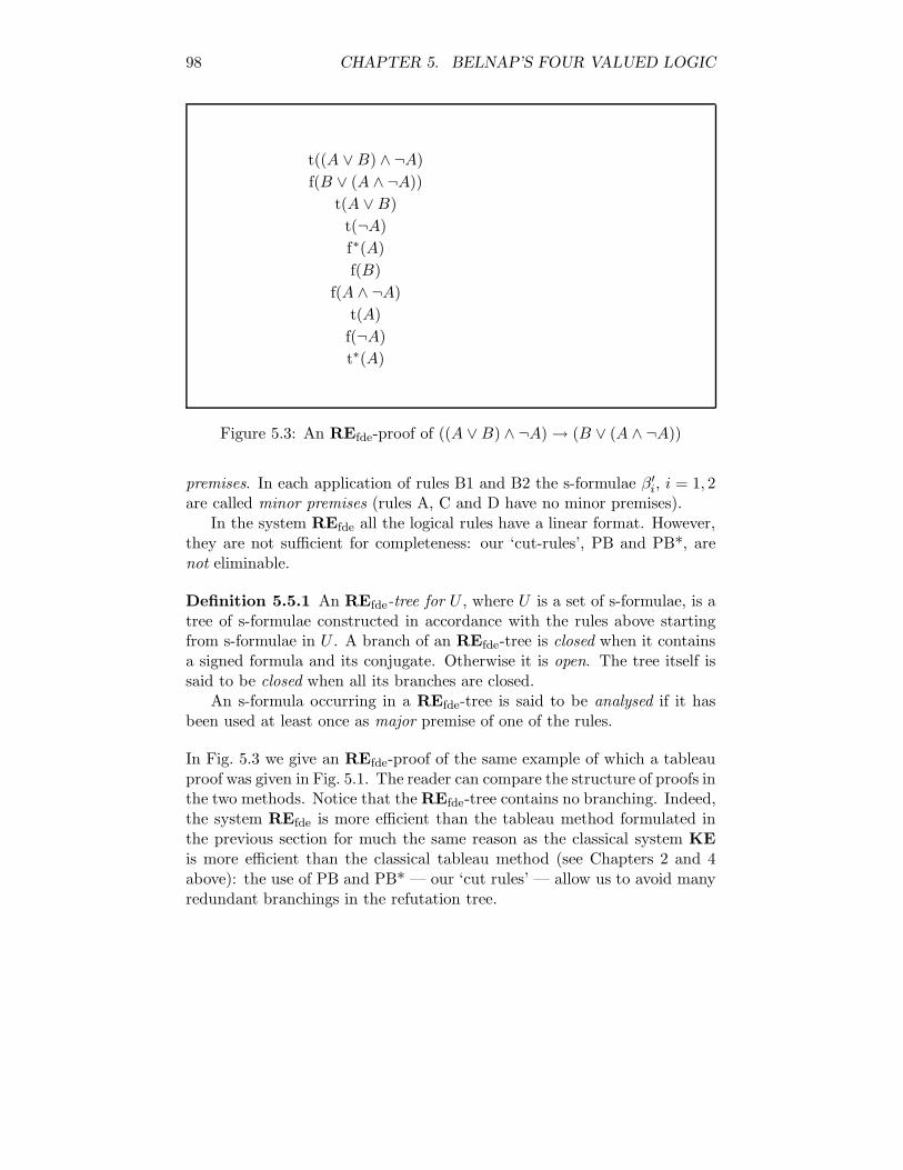
98 CHAPTER 5. BELNAP’S FOUR VALUED LOGIC
t∗(A)
f(¬A)
t(A)
f(A ∧ ¬A)
f(B)
f∗(A)
t(¬A)
t(A ∨ B)
f(B ∨ (A ∧ ¬A))
t((A ∨ B) ∧ ¬A)
Figure 5.3: An REfde-proof of ((A ∨ B) ∧ ¬A) → (B ∨ (A ∧ ¬A))
premises. In each application of rules B1 and B2 the s-formulae β′i, i = 1, 2
are called minor premises (rules A, C and D have no minor premises).In the system REfde all the logical rules have a linear format. However,
they are not sufficient for completeness: our ‘cut-rules’, PB and PB*, arenot eliminable.
Definition 5.5.1 An REfde-tree for U , where U is a set of s-formulae, is atree of s-formulae constructed in accordance with the rules above startingfrom s-formulae in U . A branch of an REfde-tree is closed when it containsa signed formula and its conjugate. Otherwise it is open. The tree itself issaid to be closed when all its branches are closed.
An s-formula occurring in a REfde-tree is said to be analysed if it hasbeen used at least once as major premise of one of the rules.
In Fig. 5.3 we give an REfde-proof of the same example of which a tableauproof was given in Fig. 5.1. The reader can compare the structure of proofs inthe two methods. Notice that the REfde-tree contains no branching. Indeed,the system REfde is more efficient than the tableau method formulated inthe previous section for much the same reason as the classical system KEis more efficient than the classical tableau method (see Chapters 2 and 4above): the use of PB and PB* — our ‘cut rules’ — allow us to avoid manyredundant branchings in the refutation tree.
5.5. AN EFFICIENT ALTERNATIVE 99
A lemma analogous to Lemma 5.4.1 holds:
Lemma 5.5.1 If T is an REfde-tree for U , where U is a set of signedformulae, then the tree T ′ obtained from T by replacing every (occurrenceof an) s-formula with (an occurrence of) its converse is an REfde-tree forthe set U∗ of the converses of the s-formulae in U .
Soundness. The proof is strictly analogous to the one given for the tableaumethod.
Completeness. We define a notion akin to the notion of R-Hintikka set :
Definition 5.5.2 Let us say that a set of signed formulae U is an R-analyticset if and only if it satisfies the following conditions:
A0: No signed variable and its conjugate are both in U .
A1: If α ∈ U , then α1 ∈ U and α2 ∈ U .
A2: If β ∈ U and β′1 ∈ U , then β2 ∈ U .
A3: If β ∈ U and β′2 ∈ U , then β1 ∈ U .
A4: If γ ∈ U , then for every k in U , γ(k) ∈ U .
A5: If δ ∈ U , then for some k in U , δ(k) ∈ U .
An R-analytic set differs from a R-Hintikka set in that it may be the casethat for some β in the set neither β1 nor β2 are in the set.
Definition 5.5.3 We say that an R-analytic set is β-complete if for everyβ in U either of the following two conditions is satisfied:
1. either β1 ∈ U or β′1 ∈ U ;
2. either β2 ∈ U or β′2 ∈ U ;
It is then easy to verify that:
Fact 5.5.1 If U is an R-analytic set and U is β-complete, then U is anR-Hintikka set.
It is not difficult to define a procedure which, given a set of s-formulaeU , generates either a closed REfde-tree or an open REfde-tree such that forevery (possibly infinite) open branch φ the set of all the s-formulae occurringin φ is a R-analytic set which is also β-complete (the only tricky part of such

100 CHAPTER 5. BELNAP’S FOUR VALUED LOGIC
a procedure concerns condition A4 and can be dealt with as in [Smu68a,pp.58–60]). Thus, completeness follows from fact 5.5.1 and lemma 5.4.4.
We can define the notions of weakly closed branch and weakly closedtree in exactly the same way as we did for the tableau method discussedin the previous section. Again the relation between classical and relevantdeducibility is the same mutatis mutandis.
Our proof of the completeness of REfde yields the subformula principleas a corollary:
Corollary 5.5.1 (Analytic Cut Property) If there is a closed REfde-tree T for U , then there is a closed REfde-tree T ′ for U such that the rulesPB and PB* are applied only to subformulae of s-formulae in U .
In fact, the proof shows that, when applying PB or PB*, we need toconsider only the immediate signed subformulae of signed formulae of typeβ occurring above in the same branch and which have not been already‘analysed’. Since all the logical rules preserve the subformula property, wehave:
Corollary 5.5.2 (Subformula Principle) If there is a closed REfde-treeT for U , then there is a closed REfde-tree T ′ for U such that every s-formulaoccurring in T ′ is a signed subformula of s-formulae in U
A constructive proof of the subformula principle, which yields a proce-dure for transforming any REfde-proof in an equivalent REfde-proof whichenjoys the subformula property, can be obtained by adapting the proof givenby Mondadori for the system KE [Mon88b].
The completeness of the (propositional fragment of the) system REfde
can also be proved by showing that all the axioms of the Hilbert-style for-mulation (given on p. 86) are theorems of REfde and REfde-derivability isclosed under the rules (8)-(11). All these facts are shown below.
In what follows ⊢ stands for ⊢REfde.
Fact 5.5.2 A ∧ B ⊢ A
(1) t(A ∧ B) Assumption(2) f(A) Assumption(3) t(A) Et∧ (1)(4) t(B) Et∧ (1)
Fact 5.5.3 A ∧ B ⊢ B
Proof as above.

5.5. AN EFFICIENT ALTERNATIVE 101
Fact 5.5.4 A ⊢ A ∨ B
(1) t(A) Assumption(2) f(A ∨ B) Assumption(3) f(A) Ef∨ (2)(4) f(B) Ef∨ (2)
Fact 5.5.5 B ⊢ A ∨ B
Proof as above.
Fact 5.5.6 A ∧ (B ∨ C) ⊢ (A ∧ B) ∨ C
(1) t(A ∧ (B ∨ C)) Assumption(2) f((A ∧ B) ∨ C) Assumption(3) t(A) Et∧ (1)(4) t(B ∨ C) Et∧ (1)(5) f(A ∧ B) Ef∨ (2)(6) f(C) Ef∨ (2)(7) t(B) Et ∨ 2 (4,6)(8) f(B) Ef ∧ 1 (5,3)
Fact 5.5.7 A ⊢ ¬¬A
(1) t(A) Assumption(2) f(¬¬A) Assumption(3) t∗(¬A) Ef¬ (2)(4) f(A) Et∗¬ (3)
Fact 5.5.8 ¬¬A ⊢ A
(1) t(¬¬A) Assumption(2) f(A) Assumption(3) f∗(¬A) Ef¬ (1)(4) t(A) Ef∗¬ (3)
Fact 5.5.9 If A ⊢ B and B ⊢ C, then A ⊢ C
It follows from the hypothesis that there are closed trees T1 and T2 for{t(A), f(B)} and {t(B), f(C)} respectively. Therefore the following is aclosed tree for {t(A), f(C)}:
t(A)f(C)
t(B) | f(B)T2 T1

102 CHAPTER 5. BELNAP’S FOUR VALUED LOGIC
Fact 5.5.10 If A ⊢ B and A ⊢ C, then A ⊢ B ∧ C
It follows from the hypothesis that there are closed trees T1 and T2 for{t(A), f(B)} and {t(A), f(C)} respectively. Therefore the following is a closedtree for {t(A), f(B ∧ C)}:
t(A)f(B ∧ C)
t(B) | f(B)f(C) T1
T2
Fact 5.5.11 If A ⊢ C and B ⊢ C, then A ∨ B ⊢ C
It follows from the hypothesis that there are closed trees T1 and T2 for{t(A), f(C)} and {t(B), f(C)} respectively. Therefore the following is aclosed tree for {t(A ∨ B), f(C)}:
t(A ∨ B)f(C)
t(A) | f(A)T1 t(B)
T2
Fact 5.5.12 If A ⊢ B, then ¬B ⊢ ¬A.
By hypothesis there is a closed trees T for {t(A), f(B)}. It follows fromLemma 5.5.1 that there is a closed tree T ′ for{t∗(A), f∗(B)}. Therefore thefollowing is a closed tree for {t(¬B), f(¬A)}:
t(¬B)f(¬A)f∗(B)t∗(A)T ′
We conclude by mentioning that a ‘naive’ implementation in Prolog of thesystem REfde has been developed by Rajev Gore [Gor90].

Chapter 6
A generalization: cut
systems
6.1 Proper derived rules
We want to address the following problem:
WHAT IS A DERIVED RULE ?
As background for our investigation we assume the Gentzen-style formaliza-tion which uses sequents, i.e. expressions of the form:
A0, A1, . . . , An ⊢ B0, B1, . . . , Bm(6.1)
with the usual meaning: if all of the Ai’s hold, then at least one of the Bi’sholds. It is convenient to treat the antecedent and the succedent as setsinstead of sequences.
By a Gentzen rule R we mean a schematic figure for passing from sev-eral sequents to another sequent, a typical example being the rule of ModusPonens:
(MP)Γ ⊢ A ∆ ⊢ A → B
Γ,∆ ⊢ B
A finite set of Gentzen rules defines a Gentzen system. Given a Gentzensystem S, there are at least three natural ways of representing proofs in it:as trees, as directed acyclic graphs or as sequences of sequents generated inaccordance with the rules of S. Whereas there is no difference in complexitybetween a proof in the form of directed acyclic graph (or ‘d.a.g.’) and a
103

104 CHAPTER 6. A GENERALIZATION: CUT SYSTEMS
proof in the form of a sequence of sequents, it is well-known that represent-ing proofs in tree-form may introduce a great deal of redundancy, becauseidentical subtrees may appear many times. However, we shall observe in thesequel that the format in which proofs are represented seems to be signifi-cant only in some special cases.
The paradigmatic Gentzen system is the calculus of sequents. There areother systems, like Natural Deduction, which can also be represented asGentzen systems, though their original formulation is not in terms of se-quents. In this chapter we restrict our attention to classical systems.
Definition 6.1.1 We say that a sequent is correct for a Gentzen system Sif and only if it is provable in S. A rule R is correct for S if and only if theconclusion of R is correct for S whenever all the premises are correct for S.
The notion of correctness of a sequent (and of a rule) makes sense even forsystems which are not formulated in terms of sequents. Given a sequentΓ ⊢ ∆, with ∆ = {A1, . . . , An}, by a single-conclusion sequent associatedwith Γ ⊢ ∆ we mean any sequent:
Γ,¬A1, . . . ,¬Ai−1,¬Ai+1, . . . ,¬An ⊢ Ai
for i = 1, . . . , n. In classical logic, every sequent is equivalent to everysingle-conclusion sequent associated with it. So, given an arbitrary proofsystem S (not necessarily formulated in term of sequents), we take as a proofof a multiple-conclusion sequent any proof of a single-conclusion sequentassociated with it, that is a proof of the single formula in the succedentfrom the formulae in the antecedent.
Let us go back to our initial problem: what is a derived rule? A first (as weshall argue, unsatisfactory) answer is the following:
(1) A rule R is a derived rule of a system S if and only if R is correct for S.
Incidentally, this answer is assumed in many logic textbooks. It is motivatedby the fact that when a rule is correct for a system S its addition to S doesnot increase the stock of provable sequents.
If we accept such a definition of derived rule, then saying that R is aderived rule of S means only that the relation ⊢ is closed under R (there isa proof of the sequent below the inference line whenever there are proofs ofthe sequents above the inference line).
¿From a proof-theoretical point of view, however, we are not interestedin the mere existence of a proof of the conclusion of a rule R, but in an

6.1. PROPER DERIVED RULES 105
effective procedure for constructing such a proof from proofs of the premises.This leads us to a different notion of derived rule:
(2) A rule R is a derived rule of S if and only if there is an effective proce-dure for constructing a proof of the conclusion of R from proofs of itspremises.
But, if we are interested in the complexity of proofs, we should also requirethat the procedure be efficient. A natural requirement, for instance, isthat the complexity of the resulting proof does not exceed the sum of thecomplexities of the component proofs plus a constant c. To make this furtherrequirement precise we can use the λ-measure used in Chapter 4:
Definition 6.1.2 The complexity of a proof π, denoted by λ(π), is the num-ber of lines in π (each ‘line’ being a sequent, a formula, or any other ex-pression associated with an inference step, depending on the system underconsideration).
We are now ready to give a definition of derived rule which takes into accountthe complexity of the procedure associated with it:
(3) An n-premise rule R is a derived rule of S if and only if there is aneffective procedure, consisting of applications of the primitive rulesof S, for constructing a proof π of the conclusion of R from proofsπ1, . . . , πn of its premises, such that λ(π) ≤ λ(π1) + · · ·+ λ(πn) + c forsome constant c.
We shall call a derived rule satisfying (3) proper derived rule.
We suggest that this notion of proper derived rule can be useful for theanalysis of the relative complexity of formal proofs. In the rest of thischapter we shall illustrate this claim in a few simple examples.
Again, we point out that the λ-measure is sufficient to establish negativeresults, but is not sufficient in general for positive results. It may, however,be adequate also for positive results whenever one can show that the lengthof lines is not significantly increased by the simulation procedure underconsideration. All the procedures that we shall consider in the sequel willbe of this kind. We assume the notions of simulation and p-simulation asdefined in Chapter 4.
Definition 6.1.3 Let us say that S′ linearly simulates S if and only if thereis a constant c such that for every S-proof π of A from Γ there is an S′-proofπ′ of A from Γ such that λ(π′) ≤ c · λ(π).

106 CHAPTER 6. A GENERALIZATION: CUT SYSTEMS
In other words λ(π′) = O(λ(π)).
The following proposition is a straightforward consequence of our definitions:
Proposition 6.1.1 Let S be a Gentzen system in tree form and S′ be anarbitrary proof system. If all the rules of S are proper derived rules of S′,then S′ linearly simulates S.
Among all the possible rules a special role is played by four rules whichare correct for an important class of logics (including, of course, the topicof this chapter: classical logic).The rule of reflexivity:
(REFL) Γ ⊢ A whenever A ∈ Γ
the rule of monotonicity
(MONO)Γ ⊢ ∆
Γ,Γ′ ⊢ ∆,∆′
the rule of substitutivity
(SUBST)Γ ⊢ ∆
sΓ ⊢ s∆
for any substitution function s (sΓ for a set Γ is defined in the obvious way),and the rule of transitivity or cut
(CUT)Γ ⊢ A,∆ Γ′, A ⊢ ∆′
Γ,Γ′ ⊢ ∆,∆′
These rules will be called common rules. They are, of course, correct forall classical systems. Since it is difficult to imagine a sensible proof systemin which REFL, MONO and SUBST are not proper derived rules, we shallrestrict our attention to systems in which they are proper derived rules andshall assume, for simplicity’s sake, that the constant c, representing the λ-complexity of the derivation of the rule, is equal to 0. On the other hand,there are well-known proof systems in which CUT, though being obviouslya correct rule (that is a ‘derived rule’ in the weak sense), is not a proper

6.2. CUT SYSTEMS 107
derived rule. Since CUT expresses the basic transitivity property of proofs,these systems can hardly claim to represent a realistic model of the notionof classical proof.
6.2 Cut systems
It is somewhat surprising how far one can go by assuming only that cut is aproper derived rule of a system. The next proposition, for example, statesthat any such system is as powerful (from the point of view of complexity)as any Frege system (another denomination of Hilbert-style proof systems).
Proposition 6.2.1 If cut is a proper derived rule of S, S linearly simulatesany Frege system.
Proof. A Frege proof π is a sequence of formulae A1, . . . , An, where An isthe theorem and Ai, i = 1, . . . , n is either an axiom or follows from previouslines by means of a rule. We shall consider axioms as rules with 0 premises.Since S is complete, then for each rule R = B1, . . . , Bm/C, m ≥ 0, there isan S-proof πR of C from B1, . . . , Bm. Let c = max(λ(πR)) for R rangingover the set of rules of the Frege system. Let An follow from Aj1, . . . , Ajk,with ji ≤ n − 1. Then, there is an S-proof of An from Aj1, . . . , Ajk and,by MONO, from A1, . . . , An−1 with λ-complexity less than or equal to c.Now, let An−1 follow from Ap1, . . . , Apq, with pi ≤ n − 2. Then there is anS-proof of An−1 from Ap1, . . . , Apq and, by MONO, from A1, . . . , An−2 withλ-complexity less than or equal to c. Since CUT is a proper derived ruleof S, there is a proof of An from A1, . . . , An−2 with complexity less than orequal to 2c + d, where d is the constant associated with the simulation ofCUT in S. It is easy to verify that by repeating this procedure we eventuallyobtain an S-proof π′ of An with λ(π′) ≤ c · λ(π) + d · (λ(π) − 1). 2
Remarks: It follows from results in [CR79] that Frege systems can poly-nomially simulate all natural deduction systems and all Gentzen systems.More recently Buss [Bus87] and Urquhart [Urq87] have shown that resolu-tion cannot polynomially simulate Frege systems. Urquhart has also shown[Urq89] that the cut-free sequent calculus in d.a.g. form cannot p-simulatethe sequent calculus with cut. Thus Proposition 6.2.1 above implies that nei-ther resolution nor the cut-free sequent calculus can p-simulate any systemin which cut is a proper derived rule.
Notice that our definition of proper derived rule does not make anyassumption about the format in which proofs are represented. In particu-lar there are many systems in tree form (including Natural Deduction and

108 CHAPTER 6. A GENERALIZATION: CUT SYSTEMS
Gentzen’s sequent calculus with cut) in which cut is a proper derived rule(or can be rendered such by means of minor transformations, see chapter 4).The proposition above then implies that neither resolution nor the cut-freesequent calculus in d.a.g. form can p-simulate any system in tree form inwhich cut is a proper derived rule.
Finally notice that the assumption that the system is classical does notplay any role in the proof. Therefore it can be extended to any logical sys-tem in which the common rules and cut are proper derived rules.
The rule of CUT we have given above is completely general and does notinvolve any logical constant. Another form of CUT which is typical of clas-sical systems is the following:
(CUT*)Γ, A ⊢ ∆ Γ′,¬A ⊢ ∆′
Γ,Γ′ ⊢ ∆,∆′
This form of cut involves the negation operator and implies that it behavesin a classical way. In classical logic the behaviour of negation is captured bytwo basic rules. The first one is also correct in intuitionistic logic:
(I¬)Γ ⊢ ∆, A
Γ,¬A ⊢ ∆
The second one is peculiar to classical logic:
(E¬)Γ,¬A ⊢ ∆
Γ ⊢ A,∆
It is easy to verify that (i) if CUT* and I¬ are proper derived rules of asystem S, so are CUT and E¬, and (ii) if CUT and E¬ are proper derivedrules of S, so are CUT* and I¬.
Definition 6.2.1 Say that a system S is a classical cut system or simply acut system if both CUT* and I¬ are proper derived rules of S or, equivalently,if both CUT and E¬ are proper derived rules of S.
We have already considered cut systems in relation to KE in chapter 4.The definition adopted there was slightly different, but can be easily provedequivalent to the present one under the assumption that the common rulesare proper derived rules. Incidentally, this is an illustration of how the

6.3. ANALYTIC CUT SYSTEMS VERSUS CUT-FREE SYSTEMS 109
notion of cut system is robust under reasonable changes of definition. Thefollowing proposition states a property of cut systems:
Proposition 6.2.2 If S is a cut system, then all the rules of Gentzen’s nat-ural deduction and sequent calculus in tree form are proper derived rules ofS. Moreover, if S enjoys the subformula property, the derivation of each ruleinvolves only formulae which are (weak) subformulae of formulae occurringin the premises or in the conclusion of the rule.
The proof is left to the reader.
6.3 Analytic cut systems versus cut-free systems
The appeal of some well-known systems in which CUT is not a proper derivedrule, like Gentzen’s sequent calculus without cut or the tableau method, ismainly due to the fact that these systems yield proofs with the subfor-mula property (SFP). In contrast, a system in which CUT is a primitiveor a proper derived rule allows for proofs without the subformula property.However, it may well be that such ‘non-analytic’ proofs are not necessaryfor completeness, i.e. that the existence of a proof with the SFP is alwaysguaranteed. This is trivially true of all systems in which CUT is eliminable.On the other hand, it is obvious that we do not need to eliminate CUT in or-der to obtain proofs with the subformula property: it is sufficient to restrictourselves to ‘analytic cuts’, i.e. to cut inferences in which the cut formulais a subformula of the assumptions or of the conclusion. It is well-knownthat the elimination of cuts can greatly increase the complexity of proofs.But we have seen in Chapter 4 that — if we consider proofs in tree-form —proofs including ‘analytic cuts’ can be essentially shorter than any equiva-lent cut-free proof while still enjoying the SFP. In particular, we have seenin Section 4.6 that any analytic cut system is essentially more efficient thanthe tableau method. For the reader’s convenience we restate this result herein a different form:
Proposition 6.3.1 Let S be any analytic cut system. Then the analyticrestriction of S linearly simulates Gentzen’s sequent calculus without cut (intree form). But Gentzen’s sequent calculus without cut (in tree form) cannotp-simulate the analytic restriction of S.
Sketch of the proof. The positive part follows from Proposition 6.1.1 andProposition 6.2.2. The negative part follows from Theorem 4.5.4 and The-orem 4.6.1.

110 CHAPTER 6. A GENERALIZATION: CUT SYSTEMS
The interest of these results lies mainly in the fact that the cut-free sequentcalculus in tree-form (or the tableau method) seems to lend itself well tocomputer search. The tree-form, in this case, is more natural. Moreover, asfar as the cut-free sequent calculus is concerned, it seems that one can findrelatively short proofs in d.a.g. or linear form only by employing the Thin-ning rule (for some results see [Urq92b]). However, as argued in Section 2.1,this rule does not suit the usual ‘bottom-up’ search procedures used in au-tomated deduction, essentially because it is not invertible. On the otherhand there are analytic cut systems, like our KE, which are as suitable forautomation as cut-free Gentzen systems but are essentially more efficient.
Chapter 7
Conclusions
Our discussion shows that KE constitutes a refutation system which lendsitself well to computer search. We propose it as an alternative both to thetableau method and resolution which combines features of both systems andremedies some of their drawbacks. It is sufficiently similar to the tableaumethod to share all its ‘desirable’ features: it does not require reduction toany normal form, obeys the subformula principle, works in the ‘analytic’ (or‘bottom-up’) direction, is ‘natural’, easy to implement and can be adaptedto a wide variety of non-classical logics. On the other hand it avoids thebasic redundancy of cut-free methods and establishes a closer connectionwith classical semantics as a result of the crucial role played by the rule PBin the analysis of the formulae of the ‘disjunctive’ (β) type. We have ex-plicitly stressed the connection between this kind of analysis and that of theDavis-Putnam procedure which is, in turn, closely related to resolution. So,from this point of view, KE can be seen as an extension of a resolution-styleanalysis to the domain of full first-order logic. Our semantic-oriented argu-ment, presented in Chapter 2, is sufficient to ensure that this kind of analysisrepresents a uniform improvement over the traditional cut-free analysis, atleast as far as the complexity of proofs is concerned. The results containedin Chapter 4 confirm and strengthen this argument in the more conventionalframework of complexity theory: the KE analysis stands with the cut-freein a relation of dominance with respect to p-simulation (KE linearly simu-lates the tableau method but the tableau method cannot p-simulate KE).Whether or not such considerations of complexity be relevant to the choiceof a formal representation for purposes other than the practical ones, is amatter which is still to be explored. Our discussion in Chapter 2, however,strongly suggests that the tableau method is not a ‘natural’ formalizationof the notion of a classical refutation and goes near to characterizing KE as
111
112 CHAPTER 7. CONCLUSIONS
the natural one.From the vantage-point of KE cut-free systems are seen as too restricted,
in a way which is not justified by their own purposes (subformula propertyand easy proof-search). Similarly, resolution is too restricted from the syn-tactical point of view: efficient classical refutations can be obtained withoutconfining ourselves to the domain of formulae in clausal form. There are, infact, connections between KE and non-clausal resolution [Mur82, MW80].However KE represents refutations in a completely different way: its rulesare genuine inference rules, in the sense that they formalize traditional in-ference principles. We have also emphasized (in Section 3.8) that KE canbe represented as a kind of ‘natural deduction’ system. Moreover, the pres-ence of a rule like PB, which can be used in a non-analytic way, makes itpossible to use KE to formalize non-analytic arguments as well as analyticones. This should be considered as an advantage from many points of view.First, as Dana Scott pointed out [Sco73], analytic logics, i.e. logics which ad-mit of formal representations that obey the subformula principle, are morean exception than the rule. Therefore KE provides a logical frameworkwhich can be extended in a natural way to non-classical logics for whicha cut-free representation is impossible. Second, even within the domainof classical logic, the possibility of representing non-analytic proofs can bean advantage. For example, it has been known since the earliest work onautomated theorem proving (see for instance [Wan60]) that biconditionalstend to cause combinatorial explosion in proof search procedures based ona cut-free Gentzen system. Recent results by Urquhart [Urq89, Urq92b]have not only proved that this phenomenon is unavoidable, but also thatthe use of analytic cut cannot help as far as pure biconditional expressionsare concerned (see Theorem 6.1 in [Urq92b]). In this case, non-analyticmethods are definitely more efficient. This is one example of the well-knownfact that using non-analytic, ‘external’, lemmata can considerably shortenproofs. Boolos [Boo84] has illustrated this fact strikingly by exhibiting anatural class of first-order schemata which have no feasible tableau proofsbut do have short natural deduction proofs. He traced the fact that naturaldeduction methods are essentially more efficient than the tableau methodto the fact that ‘modus ponens, or cut, is obviously a valid derived rule ofstandard natural deduction systems, but not obviously a valid derived rule ofthe method of trees’1, and adds that ‘the most significant feature possessedby natural deduction methods but not by the tree method, a feature thatcan easily seem like a virtue, is [. . . ] that it permits the development and
1[Boo84], p.373.

113
the utilization within derivations of subsidiary conclusions’2. Our notions of‘proper derived rule’ and ‘cut-system’, defined and used in Chapter 6, werealso meant to formalize some of the intuitions underlying Boolos’ remark.
So, there are many contexts in which purely analytic methods are hope-lessly inefficient. As Boolos himself pointed out, there is a trivial solutionto this problem: simply add cut to the cut-free rules. But this move wouldnot eliminate the redundancy of the cut-free rules that we have pointed outin Chapter 2. Moreover, the cut rule would be, so to speak, ‘thrown into’the cut-free system in a purely external way, and we would be left with noobvious criteria concerning its application. We claim that KE represents anatural and elegant solution to this problem: it does not employ any rulewhich generates redundancy in the sense of Chapter 2; the cut rule comesinto play only when the operational rules cannot be further applied; al-though its applications can be restricted to analytic ones, the unrestrictedsystem can be used to simulate efficiently all the conventional non-analyticproof systems and therefore any algorithm based on them.
Given our previous considerations, some future directions of reasearchsuggest themselves. One concerns the development of efficient proof searchprocedures for classical logic based on KE. We expect that, for analyticprocedures, some variant of Bibel’s connection method ([Bib82]; see alsothe exposition in [Wal90]), should prove useful. Similar proof-search pro-cedures for non-classical logics could be developed by adapting Wallen’smethods [Wal90]. Moreover, as suggested above, we expect KE to be usefulin formulating non-analytic proof-search algorithms both for classical andnon-classical logics, especially when non-analytic methods are the only effi-cient ones, or even, in the case of some non-classical logics, the only possibleones.
2[Boo84], p.377.

Bibliography
[AB75] A. R. Anderson and N.D. Belnap Jr. Entailment: the Logic ofRelevance and Necessity, volume 1. Princeton University Press,Princeton, 1975.
[Ajt88] Miklos Ajtai. The complexity of the pigeonhole principle. InProceedings of the 29th Annual Symposium on the Foundationsof Computer Science, 1988. Preliminary version.
[Avr88] Arnold Avron. The semantics and proof theory of linear logic.Theoretical Computer Science, 57:161–184, 1988.
[Bel76] N. D. Belnap Jr. How a computer should think. In G. Ryle,editor, Contemporary Aspects of Philosophy, pages 30–55. OrielPress, 1976.
[Bel77] N. D. Belnap Jr. A useful four-valued logic. In J. M. Dunnand G. Epstein, editors, Modern uses of multiple-valued logics,pages 8–37. Reidel, Dordrecht, 1977.
[Bet55] Evert W. Beth. Semantic entailment and formal derivabil-ity. Mededelingen der Koninklijke Nederlandse Akademie vanWetenschappen, 18:309–342, 1955.
[Bet58] Evert W. Beth. On machines which prove theorems. Si-mon Stevin Wissen Natur-kundig Tijdschrift, 32:49–60, 1958.Reprinted in [SW83], vol. 1, pages 79–90.
[BG88] Samuel R. Buss and Turan Gyorgy. Resolution proofs of gen-eralized pigeonhole principles. Theoretical Computer Science,62:311–17, 1988.
[Bib82] W. Bibel. Automated Theorem Proving. Vieweg, Braunschweig,1982.
114

BIBLIOGRAPHY 115
[Bla70] R. Blanche. La logique et son histoire. Armand Colin, Paris,1970.
[Boc61] I. M. Bochensky. A History of Formal Logic. University ofNotre Dame, Notre Dame (Indiana), 1961.
[Boo84] G. Boolos. Don’t eliminate cut. Journal of Philosophical Logic,7:373–378, 1984.
[BS89] H. A. Blair and V. S. Subrahmanian. Paraconsistent logic pro-gramming. Theoretical Computer Science, 68:135–154, 1989.
[Bus87] S. R. Buss. Polynomial size proofs of the pigeon-hole principle.The Journal of Symbolic Logic, 52:916–927, 1987.
[Car87] W.A. Carnielli. Systematization of finite many-valued logicsthrough the method of tableaux. The Journal of Symbolic Logic,52:473–493, 1987.
[Cel87] Carlo Cellucci. Using full first order logic as a programminglanguage. In Rendiconti del Seminario Matematico Universitae Politecnico di Torino. Fascicolo Speciale 1987, pages 115–152,1987. Proceedings of the conference on ‘Logic and ComputerScience: New Trends and Applications’.
[Cel88] Carlo Cellucci. Efficient natural deduction. In Temi e prospet-tive della logica e della filosofia della scienza contemporanee,volume I, pages 29–57, Bologna, 1988. CLUEB.
[Cha70] C.L. Chang. The unit proof and the input proof in theoremproving. Journal of the Association for Computing Machinery,17:698–707, 1970.
[CL73] C.L Chang and R.C.T. Lee. Symbolic Logic and MechanicalTheorem Proving. Academic Press, Boston, 1973.
[Coo71] S. A. Cook. The cmplexity of theorem proving procedures.In Proceedings of the 3rd Annual Symposium on the Theory ofComputing, 1971.
[Coo78] S. Cook. Letter to Richard Statman. Unpublished, 4, April1978.
[CR74] S. A. Cook and R. Reckhow. On the length of proofs in thepropositional calculus. In Proceedings of the 6th Annual Sym-posium on the Theory of Computing, pages 135–148, 1974.

116 BIBLIOGRAPHY
[CR79] S. A. Cook and R. Reckhow. The relative efficiency of proposi-tional proof systems. The Journal of Symbolic Logic, 44:36–50,1979.
[CS88] V. Chvatal and E. Szemeredi. Many hard examples for reso-lution. Journal of the Association for Computing Machinery,35:759–768, 1988.
[Dav83] M. Davis. The prehistory and early history of automated de-duction. In [SW83], pages 1–28. 1983.
[DCHLS90] N.C.A. Da Costa, L.J. Henschen, J.J. Lu, and V.S. Subrah-manian. Automatic theorem proving in paraconsistent logics:Theory and implementation. In M.E. Stickel, editor, LectureNotes in Artificial Intelligence, volume 449, pages 72–86, 1990.10th International Conference on Automated Deduction.
[DLL62] M. Davis, G. Logemann, and D. Loveland. A machine programfor theorem proving. Communications of the Association forComputing Machinery, 5:394–397, 1962. Reprinted in [SW83],pp. 267–270.
[DP60] M. Davis and H. Putnam. A computing procedure for quantifi-cation theory. Journal of the Association for Computing Ma-chinery, 7:201–215, 1960. Reprinted in [SW83], pp. 125–139.
[Dum78] Michael Dummett. Truth and other Enigmas. Duckworth, Lon-don, 1978.
[Dun76] J. M. Dunn. Intuitive semantics for first-degree entailment andcoupled trees. Philosophical Studies, 29:149–168, 1976.
[DW76] Bradford Dunham and Hao Wang. Towards feasible solutions ofthe tautology problem. Annals of Mathematical Logic, 10:117–154, 1976.
[FE89] L. Farinas del Cerro and P. Enjalbert. Modal resolution inclausal form. Theoretical Computer Science, 65:1–33, 1989.
[Fit83] M. Fitting. Proof Methods for Modal and Intuitionistic Logics.Reidel, Dordrecht, 1983.
[Fit87] M. Fitting. Resolution for intuitionistic logic. In Z.W. Ras andM. Zemankova, editors, Methodologies for Intelligent Systems,pages 400–407. North-Holland, Amsterdam, 1987.

BIBLIOGRAPHY 117
[Fit88] M. Fitting. First-order modal tableaux. Journal of AutomatedReasoning, 4:191–213, 1988.
[Fit90] Melvin Fitting. First-Order Logic and Automated TheoremProving. Springer-Verlag, Berlin, 1990.
[Gab90] D.M. Gabbay. Elements of algorithmic proof. In S. Abramsky,D.M. Gabbay, and T.S.E. Maibaum, editors, Handbook of Logicin Theoretical Computer Science, volume 1. Oxford UniversityPress, 1990. To appear.
[Gab91] D.M. Gabbay. Labelled deductive systems, part I. TechnicalReport CIS-Bericht-90-22, CIS-Universitat Munchen, February1991. Preliminary partial draft of a book intended for OxfordUniversity Press.
[Gal77] Z. Galil. On the complexity of regular resolution and the Davis-Putnam procedure. Theoretical Computer Science, 4:23–46,1977.
[Gal86] Jean H. Gallier. Logic for Computer Science. Harper & Row,New York, 1986.
[Gen35] Gerhard Gentzen. Unstersuchungen uber das logischeSchliessen. Math. Zeitschrift, 39:176–210, 1935. English trans-lation in [Sza69].
[Gir87a] I. Girard. Proof Theory and Logical Complexity. Bibliopolis,Napoli, 1987.
[Gir87b] J.Y. Girard. Linear logic. Theoretical Computer Science, 50:1–101, 1987.
[GJ79] M. R. Garey and D. S. Johnson. Computers and Intractability.A Guide to the theory of NP-Completeness. W.H. Freeman &Co., San Francisco, 1979.
[Gor90] Rajev Gore. Naive implementations of semantic tableaux withand without cut for classical logic, asserted 3-valued logic andBelnap’s 4-valued logic. Technical report, Cambridge UniversityComputer Laboratory, 1990. Forthcoming.
[Hak85] A. Haken. The intractability of resolution. Theoretical Com-puter Science, 39:297–308, 1985.

118 BIBLIOGRAPHY
[Hin55] Jaakko K. J. Hintikka. Form and content in quantification the-ory. Acta Philosophica Fennica, VIII, 1955.
[Jef81] Richard. C. Jeffrey. Formal Logic: its Scope and Limits.McGraw-Hill Book Company, New York, second edition, 1981.first edition 1967.
[Kal34] L. Kalmar. Uber die Axiomatisierbarkeit des Aussagenkalkulus.Acta Scient. Math. Szeged, 7:222–243, 1934.
[Kan57] Stig Kanger. Provability in logic. Acta Universitatis Stock-olmiensis, Stockolm studies in Philosophy, 1, 1957.
[Kan63] S. Kanger. A simplified proof method for elementary logic.In Computer Programming and Formal Systems, pages 87–94.North-Holland, Amsterdam, 1963. Reprinted in [SW83], pp. .
[Kar72] R.M. Karp. Reducibility among combinatorial problems. InR.E. Miller and J.W. Thatcher, editors, Complexity of Com-puter Computations, pages 85–103. 1972.
[Kle67] Stephen C. Kleene. Mathematical Logic. John Wiley & Sons,Inc., New York, 1967.
[Mat62] V. A. Matulis. Two versions of classical computation of pred-icates without structural rules. Soviet Mathematics, 3:1770–1773, 1962.
[MMO83] S. Yu. Maslov, G. E. Mints, and V.P Orevkov. Mechanicalproof-search and the theory of logical deduction in the USSR.In [SW83], pages 29–38. 1983.
[Mon88a] Marco Mondadori. Classical analytical deduction. Annalidell’Universita di Ferrara; Sez. III; Discussion paper 1, Uni-versita di Ferrara, 1988.
[Mon88b] Marco Mondadori. Classical analytical deduction, part II. An-nali dell’Universita di Ferrara; Sez. III; Discussion paper 5, Uni-versita di Ferrara, 1988.
[Mon88c] Marco Mondadori. On the notion of a classical proof. In Temie prospettive della logica e della filosofia della scienza contem-poranee, volume I, pages 211–224, Bologna, 1988. CLUEB.

BIBLIOGRAPHY 119
[Mon88d] Marco Mondadori. Sulla nozione di dimostrazione classica. An-nali dell’Universita di Ferrara; Sez. III; Discussion paper 3, Uni-versita di Ferrara, 1988.
[Mon89] Marco Mondadori. An improvement of Jeffrey’s deductive trees.Annali dell’Universita di Ferrara; Sez. III; Discussion paper 7,Universita di Ferrara, 1989.
[Mur82] N.V. Murray. Completely non-clausal theorem proving. Artifi-cial Intelligence, 18:67–85, 1982.
[MW80] Z. Manna and R. Waldinger. A deductive approach for programsynthesis. ACM Transactions on Programming Languages andSystems, 2:90–121, 1980.
[OS88] F. Oppacher and E. Suen. HARP: A tableau-based theoremprover. Journal of Automated Reasoning, 4:69–100, 1988.
[Par66] G. H. R. Parkinson, editor. Leibniz. Logical Papers. OxfordUniversity Press, 1966.
[Pra65] D. Prawitz. Natural Deduction. A Proof-Theoretical Study.Almqvist & Wilksell, Uppsala, 1965.
[Pra74] Dag Prawitz. Comments on Gentzen-type procedures and theclassical notion of truth. In A. Dold and B. Eckman, editors,ISILC Proof Theory Symposium. Lecture Notes in Mathematics,500, pages 290–319, Berlin, 1974. Springer.
[Pra78] Dag Prawitz. Proofs and the meaning and completeness of thelogical constants. In J. Hintikka, I. Niinduoto, and E. Saarinen,editors, Essays on Mathematical and Philosphical Logic, pages25–40. Reidel, Dordrecht, 1978.
[Rob65] J.A. Robinson. A machine-oriented logic based on the resolutionprinciple. Journal of the Association for Computing Machinery,12:23–41, 1965.
[Sch56] Kurt Schutte. Ein System des verknupfenden Schliessens.Archiv fur matematische Logik und Grundlagenforschung, 2:34–67, 1956.
[Sch77] Kurt Schutte. Proof Theory. Springer-Verlag, Berlin, 1977.

120 BIBLIOGRAPHY
[Sco70] Dana Scott. Outline of a mathematical theory of computation.PRG Technical Monograph 2, Oxford University ComputingLaboratory, Programming Research Group, 1970. Revised andexpanded version of a paper under the same title in the Proceed-ings of the Fourth Annual Princeton Conference on InformationSciences and Systems (1970).
[Sco73] D. Scott. Completeness and axiomatizability in many-valuedlogic. In L. Henkin, editor, Tarsky Symposium. American Math-ematical Society, 1973.
[Smu65] Raymond M. Smullyan. Analytic natural deduction. The Jour-nal of Symbolic Logic, 30:549–559, 1965.
[Smu68a] R. Smullyan. First-Order Logic. Springer, Berlin, 1968.
[Smu68b] Raymond M. Smullyan. Analytic cut. The Journal of SymbolicLogic, 33:560–564, 1968.
[Smu68c] Raymond M. Smullyan. Uniform Gentzen systems. The Journalof Symbolic Logic, 33:549–559, 1968.
[Sta77] Richard Statman. Herbrand’s theorem and Gentzen’s notion ofa direct proof. In J. Barwise, editor, Handbook of MathematicalLogic, pages 897–912. North-Holland, Amsterdam, 1977.
[Sta78] R. Statman. Bounds for proof-search and speed-up in the pred-icate calculus. Annals of Mathematical Logic, 15:225–287, 1978.
[Sti86] M.E. Stickel. An introduction to automated deduction. InW. Bibel and P. Jorrand, editors, Fundamentals of ArtificialIntelligence, pages 75–132. Springer-Verlag, 1986.
[Sto87] Larry Stockmeyer. Classifying the computational complexity ofproblems. The Journal of Symbolic Logic, 52:1–43, 1987.
[Sun83] Goran Sundholm. Systems of deduction. In D. Gabbay andF. Guenthner, editors, Handbook of Philosophical Logic, vol-ume I, chapter I.2, pages 133–188. Reidel, Dordrecht, 1983.
[SW83] Jorg Siekman and Graham Wrightson, editors. Automation ofReasoning. Springer-Verlag, New York, 1983.
[Sza69] M. Szabo, editor. The Collected Papers of Gerhard Gentzen.North-Holland, Amsterdam, 1969.

BIBLIOGRAPHY 121
[Ten78] N. Tennant. Natural Logic. Edimburgh University Press, Edin-burgh, 1978.
[Tho41] I. Thomas, editor. Greek Mathematics, volume 2. WilliamHeinemann and Harvard University Press, London and Cam-bridge, Mass., 1941.
[TMM88] P. B. Thistlewaite, M. A. McRobbie, and B. K. Meyer. Auto-mated Theorem Proving in Non Classical Logics. Pitman, 1988.
[Tse68] G. S. Tseitin. On the complexity of derivations in propositionalcalculus. Studies in constructive mathematics and mathematicallogic. Part 2, pages 115–125, 1968. Seminars in mathematics,V. A. Stkelov Mathematical Institute.
[Urq87] Alasdair Urquhart. Hard examples for resolution. Journal ofthe Association for Computing Machinery, 34:209–219, 1987.
[Urq89] A. Urquhart. The complexity of Gentzen systems for proposi-tional logic. Theoretical Computer Science, 66:87–97, 1989.
[Urq92a] A. Urquhart. Complexity of proofs in classical propositionallogic. In Y. Moschovakis, editor, Logic from Computer Science,pages 596–608. Springer-Verlag, 1992.
[Urq92b] A. Urquhart. The relative complexity of resolution and cut-free Gentzen systems. Annals of Mathematics and ArtificialIntelligence, 6:157–168, 1992.
[Wal90] L.A. Wallen. Automated Deduction in Non-Classical Logics.The MIT Press, Cambridge, Mass., 1990.
[Wan60] Hao Wang. Towards mechanical mathematics. IBM Journalfor Research Development, 4:2–22, 1960. Reprinted in [SW83],pp. 244-264.