Temporalizing Spatial Calculi:On Generalized Neighborhood Graphs

Marco Ragni and Stefan Wolfl

Institut fur Informatik, Albert-Ludwigs-Universitat Freiburg,Georges-Kohler-Allee, 79110 Freiburg, Germany

{ragni, woelfl}@informatik.uni-freiburg.de

Abstract. To reason about geographical objects, it is not only necessary to havemore or less complete information about where these objects are located in space,but also how they can change their position, shape, and size over time. In thispaper we investigate how calculi discussed in the field of qualitative spatial rea-soning (QSR) can be temporalized in order to gain reasoning formalisms that canbe used to express spatial configurations and their dynamics. In a first step, webriefly discuss temporalized spatial constraint languages. In particular, we inves-tigate how the notion of continuous change can be expressed in such languagesand how continuous change is represented in the so-called conceptual neighbor-hood graph of the spatial calculus at hand. In a second step, we focus on a specialreasoning problem, which occurs quite naturally in the context of temporalizedspatial calculi: Given an initial spatial scenario of some physical objects, whichscenarios are accessible if the set of all possible paths of these objects is con-strained by some further conditions? We show that for many spatial calculi thisgeneral problem cannot be dealt with by using the information encoded in theclassical neighborhood graphs, as usually discussed in the literature. Rather, weintroduce a generalized concept of neighborhood graph, which allows for reason-ing about objects in such dynamic settings.

1 Introduction

To reason about geographical objects, it is not only important to have information aboutwhere these objects are located in space, but also how they can change their position,shape, and size over time. Some physical objects such as chairs, towers, and stars areusually assumed to be rather robust to changes in shape and size (at least from thepoint of what we can experience without using scientific instruments). Other objectssuch as hurricanes, clouds, and balloons may vary their size and shape quite rapidly.Obviously, how physical objects can change such spatial properties depends on thephysical quality structure of the respective object and its environment. A crucial notionin this context is the notion of continuous change since it seems common-sense thatmany property changes occur continuously. Topic of the paper will be to discuss howcontinuity concepts can be integrated into the formal calculi discussed in the qualitativespatial reasoning literature.

Under the heading of qualitative spatial reasoning, many formalisms for represent-ing, and reasoning with, spatial configurations have been discussed in the past two

U. Furbach (Ed.): KI 2005, LNAI 3698, pp. 64–78, 2005.c© Springer-Verlag Berlin Heidelberg 2005

Temporalizing Spatial Calculi 65

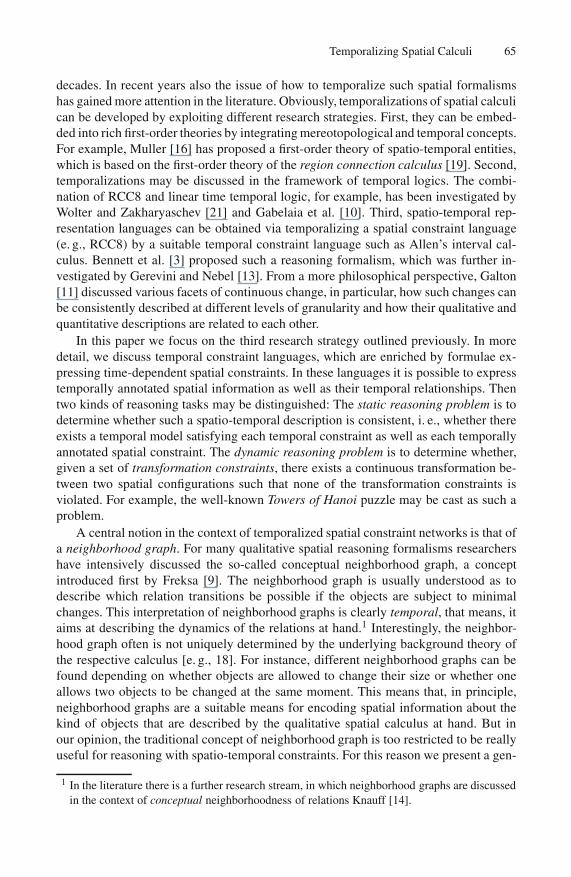
decades. In recent years also the issue of how to temporalize such spatial formalismshas gained more attention in the literature. Obviously, temporalizations of spatial calculican be developed by exploiting different research strategies. First, they can be embed-ded into rich first-order theories by integrating mereotopological and temporal concepts.For example, Muller [16] has proposed a first-order theory of spatio-temporal entities,which is based on the first-order theory of the region connection calculus [19]. Second,temporalizations may be discussed in the framework of temporal logics. The combi-nation of RCC8 and linear time temporal logic, for example, has been investigated byWolter and Zakharyaschev [21] and Gabelaia et al. [10]. Third, spatio-temporal rep-resentation languages can be obtained via temporalizing a spatial constraint language(e. g., RCC8) by a suitable temporal constraint language such as Allen’s interval cal-culus. Bennett et al. [3] proposed such a reasoning formalism, which was further in-vestigated by Gerevini and Nebel [13]. From a more philosophical perspective, Galton[11] discussed various facets of continuous change, in particular, how such changes canbe consistently described at different levels of granularity and how their qualitative andquantitative descriptions are related to each other.

In this paper we focus on the third research strategy outlined previously. In moredetail, we discuss temporal constraint languages, which are enriched by formulae ex-pressing time-dependent spatial constraints. In these languages it is possible to expresstemporally annotated spatial information as well as their temporal relationships. Thentwo kinds of reasoning tasks may be distinguished: The static reasoning problem is todetermine whether such a spatio-temporal description is consistent, i. e., whether thereexists a temporal model satisfying each temporal constraint as well as each temporallyannotated spatial constraint. The dynamic reasoning problem is to determine whether,given a set of transformation constraints, there exists a continuous transformation be-tween two spatial configurations such that none of the transformation constraints isviolated. For example, the well-known Towers of Hanoi puzzle may be cast as such aproblem.

A central notion in the context of temporalized spatial constraint networks is that ofa neighborhood graph. For many qualitative spatial reasoning formalisms researchershave intensively discussed the so-called conceptual neighborhood graph, a conceptintroduced first by Freksa [9]. The neighborhood graph is usually understood as todescribe which relation transitions be possible if the objects are subject to minimalchanges. This interpretation of neighborhood graphs is clearly temporal, that means, itaims at describing the dynamics of the relations at hand.1 Interestingly, the neighbor-hood graph often is not uniquely determined by the underlying background theory ofthe respective calculus [e. g., 18]. For instance, different neighborhood graphs can befound depending on whether objects are allowed to change their size or whether oneallows two objects to be changed at the same moment. This means that, in principle,neighborhood graphs are a suitable means for encoding spatial information about thekind of objects that are described by the qualitative spatial calculus at hand. But inour opinion, the traditional concept of neighborhood graph is too restricted to be reallyuseful for reasoning with spatio-temporal constraints. For this reason we present a gen-

1 In the literature there is a further research stream, in which neighborhood graphs are discussedin the context of conceptual neighborhoodness of relations Knauff [14].

66 M. Ragni and S. Wolfl

eralized concept of neighborhood graph, which may be considered a first step towardsdeveloping a more general theory on dynamic reasoning problems.

The paper is organized as follows: In section 2 we briefly introduce the calculi thatwill be of interest in the following sections. In section 3 we discuss spatio-temporalizedconstraint languages and their models. Moreover, we present a precise notion of con-tinuous change that enables us to analytically prove the correctness of neighborhoodgraphs. In section 4 we explain how generalized neighborhood graphs can be applied inorder to solve dynamic reasoning problems. In more detail, we present the generalizedneighborhood graphs for the point algebra and for RCC5. Finally, section 5 gives a shortsummary of our results and a brief outlook on interesting future work.

2 Preliminaries

Let us start by briefly sketching the qualitative calculi that will be of interest in thefollowing sections. Readers familiar with these calculi may wish to skip this section.

Constraint Satisfaction Problems. Qualitative reasoning problems are usually cast asconstraint satisfaction problems (CSP), i. e., as a problem to determine whether a con-straint network (a finite set of constraints) is satisfiable or entailed by another constraintnetwork. Typically, a qualitative constraint network is a finite set of constraints of theform xRy where x and y are variables taking values in a given domain D, and a binaryrelation R defined on D. For modelling imprecise knowledge, one usually considerssets of relations that are closed with respect to unions. In more detail, given a specificlevel of granularity chosen describing the domain at hand, one starts by identifing a(finite) set jointly exhaustive and pairwise disjoint sets of base relations on the domain.A composition table gives information about which constraints xRy are possible if onehas complete knowledge about how x and y are related (via base relations) to a thirdobject z. Speaking more algebraically, from a set of base relations (containing the iden-tity relation) and a composition table (satisfying some requirements), one can build upa relation algebra, i. e., a set of relations that contains the identy relation and is closedwith respect to unions, intersections, converse formation, and composition of relations.

To put these notions in a more precise context, we introduce the following terminol-ogy: A qualitative constraint satisfaction problem is defined by a constraint languageL and a class of (intended) models. The constraint language usually consists of an in-finite set of variables and a finite set of (binary) base relation symbols. A constraint isa formula of the form x{R1, . . . ,Rn}y (meaning xR1 y∨·· · ∨ xRn y), where x and y arevariables and each Ri is a base relation symbol. Finite sets of constraints are referred toas constraint networks. A model is a first- or higher-order structure M = 〈. . . ,D, . . . 〉assigning an interpretation RM ⊆ D2 to each base relation symbol R. A (variable) as-signment in M is a function a that assigns an element a(x) ∈ D to each variable x.Given an assignment a and an element d ∈ D, the function a(x/d) is defined as thefunction that coincided with a in all variables distinct from x and assigns object d tovariable x. A constraint x{R1, . . . ,Rn}y is said to be satisfied in M by a (denoted byM ,a |= x{R1, . . . ,Rn}y) if (a(x),a(y)) ∈ RM

i for some 1 ≤ i ≤ n. A constraint networkC is said to be satisfiable in a class of models if there exists a model M in this class as

Temporalizing Spatial Calculi 67

well as an assignment a in M such that all constraints in C are satisfied. Furthermore,a composition table is a map assigning to each pair of base relations Ri and R j a set ofbase relations Ri ◦R j = {Rk1 , . . . ,Rkm}. A composition table is said to be extensionallycorrect for M if for each pair of base relations Ri and R j and each assignment a,

M ,a |= x(Ri ◦R j)y ⇐⇒ ∃d ∈ D s. t. M ,a(z/d) |= xRi z and M ,a(z/d) |= zR j y.

If the base relations defined by M are (a) jointly exhaustive (i. e.,⋃

1≤i≤n RMi = D2),

(b) pairwise disjoint (i. e., RMi ∩RM

j = /0 for i = j), (c) closed with respect to converses

(i. e., RMi = (RM

j )� := {(x,y) : (y,x) ∈ RMj }), and (d) have an extensionally correct

composition table, then there exists a uniquely determined algebra of binary relationson the domain set D.

Point Algebra. The point algebra (for linear time) may be considered the most simplequalitative calculus. The point algebra (PA) describes the relations between instants oflinear flows of time. Hence, this algebra considers the three base relations < (“earlier”),= (“equal”), and > (“later”), as well as unions of them. Point algebras can also bedefined for much weaker relational structures such as branching flows of time, partialorders, etc.

Interval Algebra. Given a linear flow of time, an Allen interval is a pair of instants〈t1,t2〉 with t1 < t2. By comparing the relative positions of start and endpoints of twointervals, one can identify thirteen jointly exhaustive and pairwise disjoint base rela-tions between intervals, which are known in the literature as the Allen 13 relations (cf.Table 1).

RCC5 and RCC8. The most prominent calculi in the domain of spatial qualitative rea-soning are the region connection calculi RCC5 and RCC8. These calculi allow for

Table 1. The 13 base relations of Allen’s interval algebra

Relation Converse Pictorial Representation

I b J J bi II

J

I m J J mi II

J

I o J J oi II

J

I d J J di I IJ

I s J J si I IJ

I f J J fi I IJ

I e J J e I IJ

68 M. Ragni and S. Wolfl

X Y X YY

X YX

XY

X DR Y X PO Y X EQ Y X PP Y X PPi Y

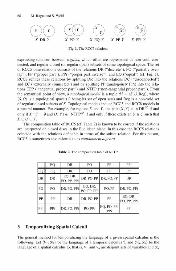
Fig. 1. The RCC5 relations

expressing relations between regions, which often are represented as non-void, con-nected, and regular closed (or regular open) subsets of some topological space. The setof RCC5 base relations consists of the relations DR (“discrete”), PO (“partially over-lap”), PP (“proper part”), PPi (“proper part inverse”), and EQ (“equal”) (cf. Fig. 1).RCC8 refines these relations by splitting DR into the relations DC (“disconnected”)and EC (“externally connected”) and by splitting PP (analogously PPi) into the rela-tions TPP (“tangential proper part”) and NTPP (“non-tangential proper part”). Fromthe semantical point of view, a topological model is a tuple M = 〈S,O,Reg〉, where〈S,O〉 is a topological space (O being its set of open sets) and Reg is a non-void setof regular closed subsets of S. Topological models induce RCC5 and RCC8 models ina natural manner: For example, for regions X and Y , the pair (X ,Y ) is in DRM if andonly if X ∩Y = /0 and (X ,Y ) ∈ NTPPM if and only if there exists an U ∈ O such thatX � U ⊆ Y .

The composition table of RCC5 (cf. Table 2) is known to be correct if the relationsare interpreted on closed discs in the Euclidean plane. In this case the RCC5 relationscoincide with the relations definable in terms of the subset relation. For this reason,RCC5 is sometimes also referred to as containment algebra.

Table 2. The composition table of RCC5

EQ DR PO PP PPi

EQ EQ DR PO PP PPi

DR DREQ, DR,

PO, PP, PPiDR,PO,PP DR,PO,PP DR

PO PO DR,PO,PPiEQ, DR,

PO, PP, PPiPO,PP DR,PO,PPi

PP PP DR DR,PO,PP PPEQ, DR,

PO, PP, PPi

PPi PPi DR,PO,PPi PO,PPi EQ, PO, PP,PPi

PPi

3 Temporalizing Spatial Calculi

The general method for temporalizing the language of a given spatial calculus is thefollowing: Let 〈VT,RT〉 be the language of a temporal calculus T and 〈VS,RS〉 be thelanguage of a spatial calculus S, that is, VT and VS are disjoint sets of variables and RS

Temporalizing Spatial Calculi 69

and RT are the sets of base relation symbols of the respective calculi. In general, thetemporal calculus will be the point algebra or the interval algebra for linear time (but,of course, the method is not restricted to these calculi). In what follows, constraints ofthe temporal calculus, i. e., formulae of the form

i{R1, . . . ,Rn} j (i, j ∈VT, R1, . . . ,Rn ∈ RT)

are referred to as temporal constraints. We now enrich the language of T by temporal-ized spatial constraints, namely formulae of the form:

i : x{S1, . . . ,Sn}y (i ∈VT, x,y ∈VS, S1, . . . ,Sn ∈ RS).

In the sequel, the combined calculus will be referred to as T :S.How can we define models for this language in terms of respective models for the

temporal and spatial languages? To illustrate this, let us start by defining the modelsof a spatial calculus chosen from the RCC-family (denoted by RCCx), which is tem-poralized by PA. The key concept for defining such models is that of a temporalizedtopological model (note that the concept used here presents a modified version of theconcept introduced by Wolter and Zakharyaschev [21]):

Definition 1. A temporalized topological model (abbr. by tt-model) is a tuple M =〈T,<,S,O,Reg,Π〉, where 〈T,<〉 is a linear flow of time, 〈S,O〉 is a topological space,Reg is a set of regions (i. e., non-void, connected, and regular closed subsets of S), andΠ is a non-void set of (object) paths π : T −→ Reg.

The idea on which the definition is based is the following: We assume that at eachinstant, an object occupies a specific region in a fixed topological space. Since we areonly interested in the path of an object, i. e., in the sequence of regions occupied by theobject, it is reasonable to represent objects as functions assigning regions to instants.

Obviously, each temporalized topological model M induces a (temporal) model forPA (denoted by MT) and a (spatial) model for RCCx (denoted by MS). A PA :RCCx(variable) assignment in a tt-model is a pair a = 〈aT,aS〉, where aT : VT −→ T is afunction assigning instants to temporal variables and aS : VS ×T −→ Reg is a functionassigning a region to each spatial variable at each instant t such that aS,x(t) := aS(t,x)defines an object path of M . Note that for each instant t, aS also defines an RCC5assignment by aS,t(x) := aS(t,x). The model relation is then introduced as follows: Fortemporal PA:RCCx constraints we set

M ,a |= i{R1, . . . ,Rn} j ⇐⇒ MT,aT |= i{R1, . . . ,Rn} j,

and for temporalized spatial constraints we define

M ,a |= i : x{S1, . . . ,Sn}y ⇐⇒ MS,aS,t |= x{S1, . . . ,Sn}y,

where t = aT(i).In the case that a spatial calculus is temporalized with respect to the interval algebra,

we need to modify this semantics as follows: An IA : RCC5 assignment in a tt-modelis a pair a = 〈aT,aS〉, where aT assigns an ordered pair (aT(i)−,aT(i)+) ∈ T 2 with

70 M. Ragni and S. Wolfl

aT(i)− < aT(i)+ to each interval variable and aS is defined as above. Here the modelrelation is defined as follows:

M ,a |= i : x{S1, . . . ,Sn}y ⇐⇒ MS,aS,t |= x{S1, . . . ,Sn}y, for eacht ∈ T with aT(i)− < t < aT(i)+.

Note that we only require that the spatial constraints hold in the interior of the interval.This is necessary since if these spatial constraints need to hold at starting and endpointsof the interval as well, then it would not be possible that a base relation holding betweenobjects X and Y in interval I changes to a different base relation between these objectsin any interval met by I. Hence, it would follow that a base relation holding betweentwo object would remain the same all the time, which is apparently unacceptable.

Let us illustrate these notions by some examples: If we temporalize the region con-nection calculus RCC5 with respect to the point algebra, we can express that two ob-jects X and Y are disjoint at some instant t, but overlap at some later instant t ′ by thefollowing constraints:

t : X DR Y, t < t ′, t ′ : X PO Y.

If we temporalize RCC8 with respect to the interval algebra, we obtain the calculusSTCC introduced by Gerevini and Nebel [13]. Here we can state constraints such as

I{m,b}J, I : X DC Y, I : Y DC Z, J : X{NTPP,TPP}Y, J : Y PO Z,

which express that interval I (weakly) precedes interval J, that during I region X isdisconnected from region Y and Y is disconnected from region Z, that during J regionX is proper part of region Y , and so on.

The semantical definitions presented so far do not impose any restrictions on howobjects can change their size, shape, or position. But how can we introduce such con-ditions on the semantic level? To explain this, let us focus on the condition that objectsneed to change their position, size, and shape continuously. For the sake of simplic-ity, we will assume that each region in a tt-model is a homeomorphic image of then-dimensional closed unit circle En (for n = 2,3) — these circles provide typical exam-ples of connected, regular closed subsets. This means that for each region X ∈ Reg, wehave a continuous function εX : En −→ S induced by a fixed homeomorphism betweenEn and X . We will be refer to such models as simple tt-models.

Definition 2. Let M be a simple tt-model. A path π : T −→ Reg of M is said to becontinuous if the function

τ : En ×T −→ S, τ(p, t) := επ(t)(p)

is continuous (in both variables, think of T as equipped with the order topology). Asimple tt-model is said to be continuous if each of its object paths is continuous, andit is strictly continuous if Π consists exactly of all continuous object paths possible forthe regions of M .

Apparently, this concept of continuous object paths is closely related to the topologi-cal notion of homotopic functions, i. e., continuous transformations between continuous

Temporalizing Spatial Calculi 71

functions. In fact, a continuous object path π defines homotopies between arbitrary re-gions π(t) and π(t ′). The important point is not that π(t) and π(t ′) are homotopic (whichis trivial since both are homeomorphic to En), but that the object path itself defines sucha homotopy. For example, let π be an object path from R into a suitable set of all subsetsof Rn assigning the unit circle to each t = 0 and the unit cube at t = 0. Then obviouslythis object path cannot be continuous.

Prepared with these notions, we can define a precise notion of the neighborhoodgraph of a spatial calculus. For this let M be a simple tt-model. We define the RCCxneighborhood graph associated to M as follows: Let S be an RCCx base relation. Theset of M -neighbors of S is defined as the smallest set of base relations, N(S), satisfyingthe following two conditions:

– S /∈ N(S);– For each pair of object paths π,π′ and each pair of instants t0 < t1 of M with

π(t0)SM π′(t0) and not π(t1)SM π′(t1), there exists a relation S′ ∈N(S) and an instantt0 < t ≤ t1 such that π(t)S′M π′(t).

Thus the RCCx neighborhood graph w. r. t. M is defined as the directed graph GRCCx,Mthat has the RCCx base relations as vertices and for each base relation an edge to eachof its M -neighbors. A graph G with vertex set RRCCx is said to be correct for a class ofmodels if G is the neighborhood graphs w. r. t. all models of that class.

Lemma 3. The neighborhood graph of RCC5 (cf. Fig. 2) is correct for each class ofstrictly continuous tt-models that instantiate all RCC5 base relations.

PP

DC PO EQ

PPi

Fig. 2. The neighborhood graph of RCC5

Given a neighborhood graph G, we define the neighborhood distance between spa-tial relations as follows: For base relations B and B′, ∆G(B,B′) is defined as the lengthof the shortest path in G between B and B′. For arbitrary relations S and S′ we set

∆G(S,S′) = minB∈S,B′∈S′

∆G(B,B′).

Obviously, ∆G(S,S′) = 0 if and only if S intersects with S′, and ∆G(S,S′) = 1 if and onlyif S and S′ are disjoint, but contain base relations B and B′ respectively such that B′ is aneighbor of B in G.

Finally, let us turn to the question whether continuity is expressible in the tempo-ralized spatial constraint language presented here. The quick answer is that continuity

72 M. Ragni and S. Wolfl

is not expressible by formulae, but is expressible via rules in the language IA:RCCx.To see this, suppose that we have a constraint set, which contains the temporalized spa-tial constraint I : X{DC,PP,EQ}Y . This constraint is satisfied by an assignment in acontinuous tt-model if and only if either I : X DC Y or I : X{PP,EQ}Y is satisfied bythat assignment. To show this, let t0 be an instant such that I− < t0 < I+ and X DC Yis false at t0, and let t1 be an arbitrary instant in the interior of I. Then we obtain thatat t1 X{DC,PP,EQ}Y is true. Without restriction we may assume that t1 < t0. Now ifX{DC}Y holds at t1, there must be an instant t1 < t ≤ t0 such that X{PO}Y is true at t.But this cannot be since at t one of the constraints X DC Y , X PP Y , or X EQ Y must betrue.

In fact, continuity rules could be applied in tableau algorithms as well as in naturaldeduction systems. But this goes beyond the scope of this paper.

4 Generalized Neighborhood Graphs

In the previous section we presented a precise notion of continuous change in spatialsettings, which can be described in terms of the RCC relations. In this section we willdeal with the question whether there exists a continuous transformation from an initialspatial scenario to a final spatial scenario, even when the set of all possible transforma-tions is restricted by some further constraints (so-called transformation constraints).

In the following, we will argue within concrete models (i. e., within the reals asflow of time and a fixed topological model such as as the Euclidean plane or the three-dimensional Euclidean space). Then the reasoning problems we are now concernedwith have the following form: Let σs and σ f be two spatial scenarios, each describingthe same set of objects X1, . . .Xn, i. e., σs and σ f are sets of “interpreted” constraintswhere between each pair of objects a spatial base relation holds. Furthermore, let Σ bea set of constraints in which at most variables for X1, . . . ,Xn occur. Now the questionis whether these objects can be continuously transformed from the first into the secondscenario so that none of the constraints in Σ is violated. In terms of Definition 1, wemay reformulate this as follows: Are there continuous paths for the objects X1, . . . ,Xn

so that the constraints of σs and σ f hold at the starting and the endpoint, respectively,and the constraints of Σ hold everywhere in the closed interval defined by starting andendpoint.

It is clear that this problem can also be expressed in terms of the temporalizedspatial constraint language presented in the previous section since a problem instance⟨Σ,σs,σ f

⟩is satisfiable in a fixed topological model if and only if the constraint set

Is m J, J m I f , Is : σs ∪Σ, J : Σ, I f : σ f ∪Σ

is satisfiable in a suitably chosen strictly continuous tt-model based on the reals and thetopological model at hand (here Is, I f , and J denote intervals: Is is an interval in whichthe start scenario holds, I f an interval in which the final scenario is true, and J is theinterval in which the transformation occurs).

Transformation problems⟨Σ,σs,σ f

⟩can easily be solved by using the informa-

tion encoded in the classical neighborhood graph of the spatial calculus at hand (e. g.,Fig. 2) if transformations of at most two objects are considered. But, in general, this

Temporalizing Spatial Calculi 73

method already fails for more than two objects. As an examples consider the scenario{X EQ Y,Y EQ Z,X EQ Z}. By only applying the information encoded in the classi-cal neighborhood graph, we cannot conclude that every change of the first constraintX EQ Y results in a change of at least one of the other two constraints [cf. 13].

The main idea to solve transformation problems is the following: Try to find a parti-tioning of the transformation interval into subintervals such that in each of these subin-tervals only a minimal number of objects has to be transformed, but the sequence ofsubintervals describes for all objects a continuous transformation from the start into thefinal scenario. This means that a transformation problem is satisfiable if there exists a se-quence of satisfiable transformation problems 〈Σ,σ1

s ,σ1f 〉, . . . ,〈Σ,σm

s ,σmf 〉 with σ1

s = σs,

σmf = σ f , and σk

f = σk+1s . This means, there is a chance to solve large and complicated

transformation problems by solving transformation problems for a restricted number ofobjects.

For such restricted problems it is interesting to precompute a generalized neighbor-hood graph, which encodes possible transformations for a fixed number of objects. Forthis we represent possible scenarios for n objects X1, . . . ,Xn as

(n2

)-tuples of spatial base

relations (Si j)1≤i< j≤n where Si j is the spatial base relation that holds between Xi and Xj

in that scenario. Note that not each such tuple is a consistent representation of a spatialconfiguration, but when it does, we will refer to it as an n-scenario. Note that, for a

spatial calculus with k relations, usually only a subset of all k(n2) many tuples represents

a scenario. For RCC5, for example, only 54 from 53 = 125 possible triples are scenariosof three objects.

Definition 4. The (n, l)-neighborhood graph (for a fixed spatial model of some spatialcalculus) is the directed graph G = (V,E) defined by the following data: V is the setof all n-scenarios and E contains a directed edge from an n-scenario s to a distinctn-scenario s′ if and only if s can be continuously transformed to s′ by changing at mostl objects.

In the case of RCC5, both the (2,1)- and the (2,2)-neighborhood graph coincidewith the classical neighborhood graph presented in Fig. 2.2 But as previously argued,a necessary condition for solving transformation problems is to solve for each triple ofobjects Xi,Xj,Xk, the transformation problem restricted to these three objects. Hence inwhat follows we focus on the (3,1)-neighborhood graph. In this graph an edge fromone vertex to another edge represents that exactly one object is subject to a continuoustransformation, while all others are considered fixed (i. e., their object paths are (locally)constant functions). If, for instance, the first object changes its position with respect tothe second object, then a scenario (r1,r2,r3) can be connected to (r′1,r

′2,r

′3) only if (in

the classical neighborhood graph) ∆(r1,r′1) = 1, ∆(r2,r′2) = 0, and ∆(r3,r′3) ≤ 1.The (3,1)-neighborhood has the nice feature that it can be computed easily by ex-

tensively using the information encoded in the classical neighborhood graph and in thecomposition table of the spatial calculus at hand. More precisely, the algorithm GNGpresented in Fig. 3 takes as input a list of base relations (denoted by rel list[ ]) and anarray representing the composition table (compTable[i][ j] refers to the set of base re-

2 Note that the (2,1)- and the (2,2)-neighborhood are not necessarily identical [cf. 18].

74 M. Ragni and S. Wolfl

lations obtained by composing relations i and j). The function neighbor(i) assigns toeach base relation its set of neighbors w. r. t. the classical neighborhood graph.

The algorithm GNG works as follows: First, it generates a possible scenario (i, j,k),checks if it is consistent. If so, it calls a function that generates a list of all continu-ous successors of the scenario (i, j,k). Finally, this list is returned. In more detail, theBoolean function isConsistent() checks for a triple (i, j,k), whether k is contained incompTable[i][ j], in other words, whether relation k can hold between objects X and Y ifthere exists an object Z such that X iZ and Z jY are true. The function Succ() generatesfor a triple (i, j,k) all consistent successors into which the scenario can be transformed.This is done in the following way: For the input (i, j,k) the algorithm successively gen-erates a neighbor relation for each relation of the triple. If, for instance, l is a neighborrelation of i, the algorithm checks if (l, j,k) is consistent. If so, the relation is added tothe list of possible successors. This models the qualitative change of object X in relationto some fixed objects Y and Z. By changing object X , its qualitative relation to Z canalso be affected. Since in this case object Y and Z are considered fixed, the relation jcannot change. The same is analogously done for the second and third relation of thetriple.

Proposition 5. The (3,1)-neighborhood graph computed by the algorithm GNG is (se-mantically) correct, if the algorithm is applied to a correct (2,1)-neighborhood graphand a correct composition table.

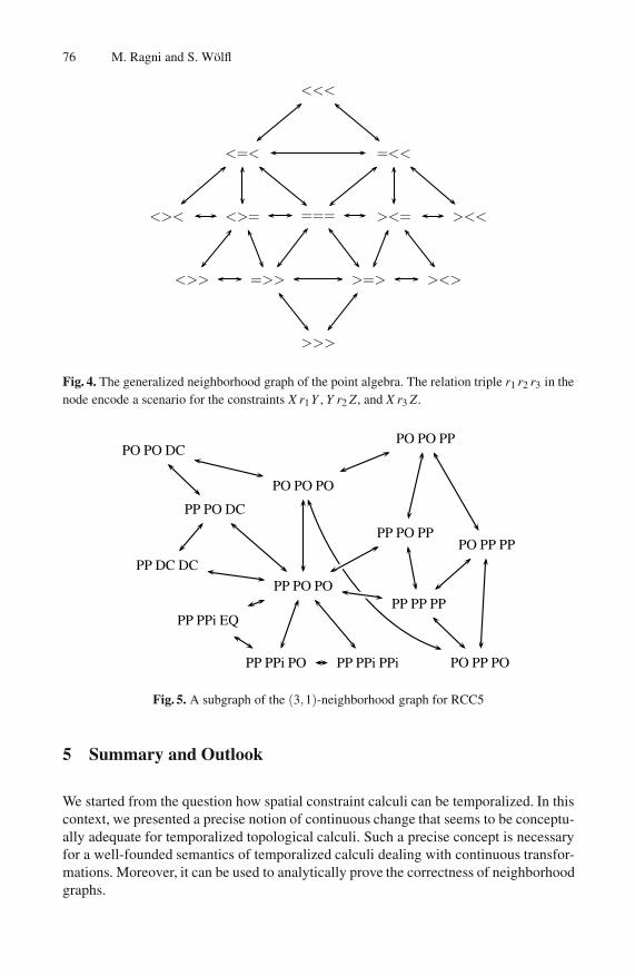
By applying this proposition to Lemma 2 we obtain that for RCC5 the (3,1)-graphcomputed by GNG is correct for each class of strictly continuous tt-models that instan-tiate all base relations. This graph (a subgraph of it is depicted in Fig. 5) has 54 verticesand 291 edges.3 We also applied this algorithm for computing the (3,1)-neighborhoodgraphs of the point algebra (PA) thought of as a spatial calculus. In this case the graphconsists of 13 vertices and 24 edges (cf. Fig. 4).

To put things a little bit further, we can define a refined consistency concept fortransformation problems.

Definition 6. A transformation problem⟨Σ,σs,σ f

⟩is said to be (n, l)-consistent if for

each subscenario of σs consisting of n objects X1, . . . ,Xn, there exists a path in the(n, l)-neighborhood graph to the corresponding subscenario of σ f (the subscenario forX1, . . . ,Xn) such that no constraint of Σ is violated.

This consistency concept can be useful, when impossible transformations are to beidentified. Since a problem instance with m objects is satisfiable only if it is (n, l)-consistent for all n, l ≤ m, we can apply the (n, l)-neighborhood graph in order tofind impossible transformations. To illustrate this, let us discuss the following exam-ple for the point algebra: Consider the PA-scenarios σs = {a < b,b < c,a < c} andσ f = {a < b,b > c,a < c}. Can σs be transformed into σ f if we forbid that b = c, i. e.,b{<,>}c∈ Σ? Certainly not, because a lookup in the (3,1)-neighborhood graph showsthat there is no path between the corresponding vertices. This can of course also be used

3 A representation of the full (3,1)-neighborhood graph for RCC5 is available to the public atftp://ftp.informatik.uni-freiburg.de/documents/papers/ki/ragni-woelfl-nghood.pdf.

Temporalizing Spatial Calculi 75

def GNG ( rel list [ ], compTable[ ][ ])for i, j,k in rel list[ ]:

if isConsistent (i, j,k) :Succ(i, j,k)

else :output “scenario (i, j,k) is inconsistent”;

output “all successors of (i, j,k)”: Succ(i, j,k);

def function isConsistent (i, j,k)if k ∈ compTable[i][ j]:

return true ;else return false ;

def function Succ(i, j,k)succArray[ ];for l ∈ {i, j,k}:

if l = i :for m ∈ neighbor(i):

if isConsistent (m, j,k) && (m, j,k) /∈ succArray[ ]:succArray[ ] = succArray[ ]∪ (m, j,k);

for n ∈ neighbor(k):if isConsistent (m, j,n) && (m, j,n) /∈ succArray[ ]:

succArray[ ] = succArray[ ]∪ (m, j,n);if l = j :

for m ∈ neighbor( j):if isConsistent (i,m,k) && (i,m,k) /∈ succArray[ ]:

succArray[ ] = succArray[ ]∪ (i,m,k);for n ∈ neighbor(i):

if isConsistent (n,m,k) && (n,m,k) /∈ succArray[ ]:succArray[ ] = succArray[ ]∪ (n,m,k);

if l = k:for m ∈ neighbor(k):

if isConsistent (i, j,m) && (i, j,m) /∈ succArray[ ]:succArray[ ] = succArray[ ]∪ (i, j,m);

for n ∈ neighbor( j):if isConsistent (n, j,m) && (n, j,m) /∈ succArray[ ]:

succArray[ ] = succArray[ ]∪ (n, j,k);output succArray[ ]

Fig. 3. The algorithm GNG computes the (3,1)-neighborhood graph from a set of base relations,a composition table, and a classical neighborhood graph

in more complex formal calculi. For a given transformation problem, check first if foreach pair of objects X and Y with X r1 Y ∈ σs and X r2 Y ∈ σ f , there is a path from r1

to r2 in the classical neighborhood graph. Then for each triple of objects X , Y , and Zwith X r1 Y,Y r2 Z,X r3 Z ∈ σs and X r′1 Y,Y r′2 Z,X r′3 Z ∈ σ f , check if there is a path inthe (3,1)-, (3,2)-, or (3,3)-neighborhood graph from (r1,r2,r3) to (r′1,r

′2,r

′3) so that

during that none of the constraints in Σ is violated, and so on.

76 M. Ragni and S. Wolfl

<<<

<=< =<<

<>< <>= === ><= ><<

<>> =>> >=> ><>

>>>

Fig. 4. The generalized neighborhood graph of the point algebra. The relation triple r1 r2 r3 in thenode encode a scenario for the constraints X r1Y , Y r2 Z, and X r3 Z.

PO PO PO

PP PO PO

PP PO DC

PP DC DC

PP PPi EQPP PP PP

PP PPi PPi

PP PO PP

PP PPi PO

PO PP PP

PO PP PO

PO PO DCPO PO PP

Fig. 5. A subgraph of the (3,1)-neighborhood graph for RCC5

5 Summary and Outlook

We started from the question how spatial constraint calculi can be temporalized. In thiscontext, we presented a precise notion of continuous change that seems to be conceptu-ally adequate for temporalized topological calculi. Such a precise concept is necessaryfor a well-founded semantics of temporalized calculi dealing with continuous transfor-mations. Moreover, it can be used to analytically prove the correctness of neighborhoodgraphs.

Temporalizing Spatial Calculi 77

In a second step we considered so-called transformation problems, i. e., problems ofthe kind whether some spatial configuration can be continuously transformed into an-other configuration, even if these transformations are constrained by further conditions.Solving such problems may be especially interesting, for instance, if we want to planhow objects have to be moved in space in order to reach a specific goal state.

The classical neighborhood graphs discussed in the literature only represent pos-sible continuous transformations of at most two objects. We proposed a concept thateliminates this limitation. These generalized neighborhood graphs may also be consid-ered an appropriate tool for solving transformation problems, because they mirror thenotion of k-consistency known from static reasoning problems. This idea is reflected inour definition of (n, l)-consistency.

Future work will be concerned with the following questions: What is the exact rela-tionship between (n, l)-consistency and satisfiability of transformation problems? Arethere tractable classes of these problems? How can the notion of (n, l)-consistency beused to identify such classes? Finally, how can temporalized QSR be used to solvespatial planning scenarios?

Acknowledgments

This work was partially supported by the Deutsche Forschungsgemeinschaft (DFG) aspart of the Transregional Collaborative Research Center SFB/TR 8 Spatial Cognition.We would like to thank Bernhard Nebel for helpful discussions. We also gratefullyacknowledge the suggestions of three anonymous reviewers, who helped improving thepaper.

References

[1] J. F. Allen. Maintaining knowledge about temporal intervals. Communications of the ACM,26(11):832–843, 1983.

[2] B. Bennett. Space, time, matter and things. In FOIS, pages 105–116, 2001.[3] B. Bennett, A. G. Cohn, F. Wolter, and M. Zakharyaschev. Multi-dimensional modal logic

as a framework for spatio-temporal reasoning. Applied Intelligence, 17(3):239–251, 2002.[4] B. Bennett, A. Isli, and A. G. Cohn. When does a composition table provide a complete

and tractable proof procedure for a relational constraint language? In Proceedings of theIJCAI97 Workshop on Spatial and Temporal Reasoning, Nagoya, Japan, 1997.

[5] A. G. Cohn. Qualitative spatial representation and reasoning techniques. In G. Brewka,C. Habel, and B. Nebel, editors, KI-97: Advances in Artificial Intelligence. Springer, 1997.

[6] E. Davis. Continuous shape transformation and metrics on regions. Fundamenta Informat-icae, 46(1-2):31–54, 2001.

[7] M. J. Egenhofer and K. K. Al-Taha. Reasoning about gradual changes of topological rela-tionships. In A. U. Frank, I. Campari, and U. Formentini, editors, Spatio-Temporal Reason-ing, Lecture Notes in Computer Science 639, pages 196–219. Springer, 1992.

[8] M. Erwig and M. Schneider. Spatio-temporal predicates. IEEE Transactions on Knowledgeand Data Engineering, 14(4):881–901, 2002.

[9] C. Freksa. Conceptual neighborhood and its role in temporal and spatial reasoning. In De-cision Support Systems and Qualitative Reasoning, pages 181–187. North-Holland, 1991.

78 M. Ragni and S. Wolfl

[10] D. Gabelaia, R. Kontchakov, A. Kurucz, F. Wolter, and M. Zakharyaschev. Combiningspatial and temporal logics: Expressiveness vs. complexity. To appear in Journal of ArtificialIntelligence Research, 2005.

[11] A. Galton. Qualitative Spatial Change. Oxford University Press, 2000.[12] A. Galton. A generalized topological view of motion in discrete space. Theoretical Com-

pututer Science, 305(1-3):111–134, 2003.[13] A. Gerevini and B. Nebel. Qualitative spatio-temporal reasoning with RCC-8 and Allen’s

interval calculus: Computational complexity. In Proceedings of the 15th European Confer-ence on Artificial Intelligence (ECAI-02), pages 312–316. IOS Press, 2002.

[14] M. Knauff. The cognitive adequacy of allen’s interval calculus for qualitative spatial repre-sentation and reasoning. Spatial Cognition and Computation, 1:261–290, 1999.

[15] P. Muller. A qualitative theory of motion based on spatio-temporal primitives. In A. G.Cohn, L. K. Schubert, and S. C. Shapiro, editors, Proceedings of the Sixth InternationalConference on Principles of Knowledge Representation and Reasoning (KR’98), Trento,Italy, June 2-5, 1998, pages 131–143. Morgan Kaufmann, 1998.

[16] P. Muller. Topological spatio-temporal reasoning and representation. Computational Intel-ligence, 18(3):420–450, 2002.

[17] B. Nebel and H.-J. Burckert. Reasoning about temporal relations: A maximal tractable sub-class of Allen’s interval algebra. Technical Report RR-93-11, Deutsches Forschungszen-trum fur Kunstliche Intelligenz GmbH, Kaiserslautern, Germany, 1993.

[18] M. Ragni and S. Wolfl. Branching Allen: Reasoning with intervals in branching time. InC. Freksa, M. Knauff, B. Krieg-Bruckner, B. Nebel, and T. Barkowsky, editors, SpatialCognition, Lecture Notes in Computer Science 3343, pages 323–343. Springer, 2004.

[19] D. A. Randell, Z. Cui, and A. G. Cohn. A spatial logic based on regions and connection.In B. Nebel, W. Swartout, and C. Rich, editors, Principles of Knowledge Representationand Reasoning: Proceedings of the 3rd International Conference (KR-92), pages 165–176.Morgan Kaufmann, 1992.

[20] M. B. Vilain, H. A. Kautz, and P. G. van Beek. Contraint propagation algorithms for tem-poral reasoning: A revised report. In D. S. Weld and J. de Kleer, editors, Readings inQualitative Reasoning about Physical Systems, pages 373–381. Morgan Kaufmann, 1989.

[21] F. Wolter and M. Zakharyaschev. Spatio-temporal representation and reasoning based onRCC-8. In A. Cohn, F. Giunchiglia, and B. Selman, editors, Principles of Knowledge Rep-resentation and Reasoning: Proceedings of the 7th International Conference (KR2000).Morgan Kaufmann, 2000.