
A conceptual framework for comparing instructional design models
Upload
independentCategory
view
4download
0
J. Symbolic Computation (1994) 11, 1–000
Consolution as a Framework for Comparing Calculi
PETER BAUMGARTNER and ULRICH FURBACH
University of Koblenz, Rheinau 1,
56075 Koblenz, Germany�peter,uli� @informatik.uni-koblenz.de
(Received 20 May 1994)
In this paper, stepwise and nearly stepwise simulation results for a number of first-order proof calculiare presented and an overview is given that illustrates the relations between these calculi. For thispurpose, we modify the consolution calculus in such a way that it can be instantiated to resolution,tableaux model elimination, a connection method and Loveland’s model elimination.
1. Introduction
In (Eder, 1991) the consolution method is introduced as a bridge between the idea of matrixmethods (see (Bibel, 1987)) and resolution. Eder defines a consolution calculus together witha construction which yields a consolution refutation for every resolution refutation. This givesboth a demonstration that resolution can be seen as a special strategy within consolution anda completeness proof for consolution. However, Eder did not investigate a formal treatment ofmatrix methods with consolution; he only gave an informal description of matrix methods as astarting point for consolution.
It appeared fascinating to us to see how easily the two ideas of a matrix method and a resolutioncalculus can be combined in the consolutionmethod. We tried to followthis line to use consolutionas a framework to relate matrix methods and resolution by defining special consolution calculi.It turned out that this is not as straightforward as we expected. However we can reach this goalby making numerous changes to the definition of consolution. The changes are harmless in thesense that the inference rules of the modified calculus subsume that of the original calculus. Thedocumentation of these changes is one purpose of this paper.
Another purpose is to demonstrate that consolution is well suited for comparing calculi. Thisis a topic of significant importance for anyone trying to understand the essence of deduction orto implement a deduction system.
In particular we show that when defined appropriately, consolution can simulate step by stepa certain model elimination calculus (model elimination as defined by Loveland), a connectionmethod calculus and a tableau model elimination calculus on which proof procedures like PTTP(Stickel, 1989; Stickel, 1988) and SETHEO (Letz et al., 1992) are based. The result for resolutionand consolution was shown in (Eder, 1991). Altogether we will prove the diagram from figure1, where the � � � means that calculus � can be simulated stepwise by calculus � ; dashedarrows indicate a “weaker” simulatability relation after certain calculus restrictions.
0747–7171/90/000000 + 00 $03.00/0 c�
1994 Academic Press Limited

2 P. Baumgartner and U. Furbach
� � � � � � � � � � � � �
� � � � � � � � � � � �
����
����
����
Connection
Sequence Consolution
Resolution Calculus
Tableau-Model-Elimination
Loveland’sModel-Elimination
Consolution
Figure 1. Relations between calculi.
Furthermore all these calculi are defined in a uniform and consolution-like language, making iteasy to relate them among each other. This is a significant difference when compared with otherwork — we use one formal framework for the definition of the various calculi, which allowsrigorous comparisons together with proofs.
In the next section we briefly review the idea and the consolutioncalculus as it is given in (Eder,1991). In section 3 we define a model elimination calculus in a consolution-like language, whichwe call “tableau model elimination”, and show how to modify consolution in order to simulatetableau model elimination. As a result we come up with a consolution method called “sequenceconsolution”which loses part of its elegance and simplicity compared with the original, but whichmakes some of its parameters explicit. Section 4 relates consolution to sequence consolution in aformal way. Sequence consolution then serves as a framework for the definition and comparisonof other calculi. This is done in section 5 for Loveland’s original model elimination calculus andin section 6 for a connection calculus. Section 7 relates the tableau model elimination calculus toresolution. Finally section 8 contains the discussion.
2. The Idea of Consolution
Consolution can be seen as a procedure for converting a formula given in one normal forminto another normal form: assume we are given a (for simplicity: ground) formula in disjunctivenormal form (DNF) and want to prove its validity. This can be done by converting it in a first stepinto conjunctive normal form (CNF). The second step then uses the fact that a formula in CNF isvalid iff every conjunct contains complementary literals. Thus, a simple test for complementaryliterals in every conjunct suffices to decide the validity of the CNF and also the DNF. Now,with some additional optimizations this is just how consolution works. Consider for example theDNF-formula � � � � � � �
� � � �
� � �
�

Consolution as a Framework for Comparing Calculi 3
Conversion to CNF can be begun by applying the law of distributivity to the underbraced part,yielding � � � �
� � � � � � � � � � � �
� � � � � � � � � �
�
This operation is also carried out as a first step in an consolution inference. The subsequent stepsdeal with the above-mentioned optimizations: first, disjuncts such as
� �
�which contain
complementary literals are tautological and thus can be removed. Second, disjuncts may beshortened; for example,
� � �
� �may be replaced by
�. This corresponds in some sense to
the “weakening” rule in Gentzen’s sequent calculus (see e.g. (Gallier, 1987) for the sequentcalculus). The shortening step is sound since it preserves non-tautologyhood. However, it maycause incompleteness by throwing away the “wrong” literal, i.e. the literal that contributes to acomplementary pair in a later stage. Third,
� � �can be replaced by
�. This rule corresponds to
the “contraction” rule in the sequent calculus. It is implicitly present in consolution by means ofthe set data structure, which collapses multiple occurences of literals into a single one. Similarly,identical conjuncts such as
�in
� � �can be contracted to a single one. Carrying out these
suggested operations results in the formula� � � � � � � � � �
�
This formula is the result of an application of the consolution inference rule. Applying the ruleagain yields by the law of distributivity the formula� � � � �
� � � � � �
� �
This formula can be simplified as explained above towards the “empty” conjunct, which is aproof for the validity of the given formula.
Consolution is slightly more general than just explained: instead of logical formulas in DNF,consolution works on sets of clauses, where a clause is a set of literals. The semantics of clausesets is then obtained by interpreting the outer commas by “
�” and the inner commas by “
�”.
The clause set data structure is more general, since the interpretation of the outer comma andinner comma can be exchanged. In other words, one starts with a CNF instead of a DNF. Aderivation of the empty clause can then be interpreted as proof of the unsatisfiablity of the DNF-formula, instead of a proof of the validity of a (logically different) CNF-formula. This dualityis not specific to consolution but applies to every calculus with clause sets as data structure. Itgives us the freedom to directly relate derivations in e.g. model elimination (which is usuallyformulated in the refutational setting) and consolution (which was formulated in Eder’s theoremin the affirmative setting).
Consolution can also be explained from the background of the connection method (cf. (Bibel,1987)). Here, sets of clauses are called matrices, and the method is concerned with proving thatevery path through this matrix contains two complementary literals, called connections in thisframework (a path through a matrix is built by selecting exactly one literal from every clause inthe matrix).
To illustrate consolution we use an example from (Eder, 1991):The three clauses �
��
� �, �
��
� �and
�are represented in the connection method as a
matrix � :

4 P. Baumgartner and U. Furbach
��
��
�
Thus the possible paths through this matrix are ��
� �
� � �
, ��
��
� � �
, ��
� �
� � �
and��
� � �
. Consolution shares with the connection method the idea of showing that every pathcontains a connection. Consolution does so by combining partial paths through a matrix to evenlonger partial paths and thereby ruling out paths containing a connection. The following tree isa proof tree in consolution. The nodes are marked with path sets, e.g. � �
��
� �� �
��
� �� �
� � �is a set with three partial paths through the two leftmost clauses in the matrix � . Now, in aninference the cross product of the elements of the parent nodes is built, and paths containingconnections are deleted.
� �� �
� �� � �
� � � �
� �� � �
� ��
�� �
� ��
� � �
� �� � �
� � � � �
��
� � � � � � � � � � � � � �
� � � � � � � � � � � � � � � �
The root of this tree is the empty path set, which proves that all paths through � are comple-mentary.
To introduce consolution formally we need only the following definitions.A connection in a set of clauses or a matrix is a pair
� � � ��
of literals which can be madecomplementary by application of a substitution.
DEFINITION 2.1. (Eder’s Consolution (Eder, 1991)) A path is a finite set of literals.If p and q are paths and � and � are path sets, then pq :� p q and � � :� � pq � p �� and q � �
�. For ease of notation we write p � as an abbreviation for � p
� � . If C is a clause
then its path set is � C :� � � L
�� L � C
�.
A path set � is obtained from a path set � by elimination of complementary paths if thereis a set of connections in � and a most general unifier of this set of connections such that �is the set of non-complementary elements in � . A path set � is obtained from a path set � byshortening of paths if there is a surjective mapping f : � � � such that f
�p
� �p holds for all
p � � .A path set � is obtained from a path set � by simplification (Version 0)� if there exists a path
set � such that � is obtained from � by elimination of complementary paths and such that � isobtained from � by shortening of paths.
The inference rule consolution is defined as follows� ��
�Later on we will introduce different versions of simplification.
Consolution as a Framework for Comparing Calculi 5
if there exists a variant � � of � which does not have variables in common with � such that � isobtained from � � � by simplification. � is called a consolvent of � and � .
�
To recognize the soundness of the consolution inference rule consider again the explanation atthe beginning of the previous section. In particular, multiplication of paths corresponds to theapplication of the law of distributivity, which is an equivalence transformation. Furthermore,if path sets are interpreted as conjunctions of disjunctions then shortening of paths preservesnon-tautologyhood; or dually, if path sets are interpreted as disjunctions of conjunctions thenshortening of paths preserves satisfiability.
DEFINITION 2.2. (Derivation) A derivation of a matrix M is a finite sequence
�� 1 � � � � � � n
�of
path sets, where n � 1 and for all k � 1 � � � � � n the set � k equals � C for some C � M, or � k is aconsolvent of � i and � j for some i � j � k. A derivation ending in a path set � n � � is also called
a refutation.� �
The reader is invited to figure out in detail the derivation which led to the consolution prooftree given above.
THEOREM 2.1. (Eder, 1991) A formula in disjunctive normal form is valid if and only if there isa refutation of its matrix by consolution.
Eder gave a proof of this theorem which used the completeness of resolution. The proofis by constructing a consolution derivation for every resolution refutation, which gives thecompleteness of consolution (see theorem 8.1 in section 8).
3. Model Elimination and Consolution
In this section we will informally introduce a model elimination calculus. Then a formalizationin a consolution-like language follows. Building on this, we define a more refined consolutionmethod, which can then be shown to simulate stepwise the model elimination calculus.
Model elimination was originally introduced by Loveland (cf. (Loveland, 1968; Loveland,1969; Loveland, 1978)). It can be seen as a restricted form of linear resolution (see (Loveland,1978) and section 7). However, model elimination and its linear proof format was invented beforelinear resolution, which came up in 1970. More recently it became obvious that model eliminationcan be understood very naturally as a matrix method; here we will follow the lines from (Letzet al., 1992) and define the inference rules as tree-transforming operators. Then the calculus ismuch in the spirit of semantic tableaux with unification for clauses (see (Fitting, 1990)), but withan important restriction. This restriction will be explained below and justifies using the new name— “tableau model elimination” — instead of qualifying it as “analytical tableaux for clauses withunification”.
Compared to Loveland’s model elimination, the calculus presented below is weaker, in that itlacks some efficiency improvements. Of course, these could be added, but for our purpose theyare not essential and hence are omitted for the sake of simplicity.
As an example for model elimination in our format take the following tree, which is nothingmore than a representation of the clause �
��
� �of the matrix � in the consolution example.�
Here we are not compatible with (Eder, 1991). What he calls “derivation” is called “refutation” by us; this was doneto be compatible with subsequent calculi and to standard text books (e.g. (Chang and Lee, 1973)).

6 P. Baumgartner and U. Furbach
� ��
��
��
��
��
�
An extension step can be performed by selecting one branch of the tree, say the one leading to�, and an input clause that contains a literal which can be made complementary by unification
with the leaf of that path; in the notation of matrix methods this is a connection. In our examplethe clause �
��
� �can be used to construct a new tree:
� �
�
�
�
��
��
�� �
��
��
�
��
��
���
��
��
The selected path is extended with the literals of the clause as new leaves. As usual, the groundcase for the connection is lifted to the general case by means of a most general unifier (MGU),and this unifier has to be applied to the entire tree. As a result of this operation, (at least) oneextension of the selected path contains complementary literals and can be closed, i.e. it need notbe considered further; this is marked with an asterisk. The other extensions remain unmarked.However, closing a branch can be achieved even without extending the tree with a new clause:whenever a leaf of a path has a connection with one of its ancestor literals, the path may be closedand the used MGU is applied to the entire tree. Such steps are called reduction steps. Unlessthe used MGU is empty there is a don’t-know nondeterminism here wrt. the application of anextension step or a reduction step.
In our example, after two more extension steps we arrive at a tree which contains only closedpaths, and thus serves as a refutation:
� �
�
�
�
��
�
�
��
��
��
� � � � � � � � ��
��
��
���
��
��
Let us use now the notation from consolution to describe tableau model elimination. Sinceconsolution manipulates sets of paths our trees should be coded as consolution path sets. Then,neglecting already closed paths, for example, the second tree in the derivation above is naturallyrepresented by the path set � � � �
��
� �� �
� � �. For the extension step we have to select one
path, say ��
�� �
, and within that path we have to select the leaf as part of a connection. Butwhich element of the set is the leaf? Due to set notation, the information about which literal isthe leaf is lost. What we need are paths as sequences instead of sets:

Consolution as a Framework for Comparing Calculi 7
DEFINITION 3.1. (Path) A path is a sequence of literals, written as p � L1 � � Ln. Ln is calledthe leaf of p, which is also denoted by leaf
�p
�. By abuse of notation, ‘� ’ denotes also the append
function for literal sequences.The operations “elimination of complementary paths” and multiplication (“ ”) are modified as
expected.A path q is obtained from a path p � L1 � � Ln by immediate shortening of p, q � p, iff
�i
�1 � i � n
�: q � L1 � � Li� 1 � Li� 1 � � Ln
For the transitive closure we say that q is obtained by shortening of p iff q � � p.The partial order � on paths is defined as
p � q iff p � q or else p � � q
The definition of shortening of paths (cf. def. 2.1) is modified to take care of the new datastructure: a path set � is obtained from a path set � by shortening of paths if there is a surjectivemapping f : � � � such that f
�p
�� p holds for all p � � .
�
Now, when using sequences instead of sets we can identify a leaf in a path, i.e. in the firstextension step of the above example we take in consolution the path
�and multiply it with the
path set � �
�� �
, which is derived from the clause � �
�� �
. This gives ��
� �
��
�
� �; to
get the closing effect from model elimination in consolution, we have to choose only connectionswe have just introduced during the multiplication. (In this example this is the only one). Then wehave to apply the unifier for these connections to the path set and subsequently have to eliminatecomplementary paths. In our case the only complementary path we want to eliminate is the onewhich contained the connection chosen for this step.
Another property of tableau model elimination is that it only manipulates one path at a time,even if there are identical paths within a tableau. Thus, the paths of a tableau model eliminationtree are technically a multiset. In consolution however we deal with sets of paths. In otherwords, multiple occurrences of identical paths in model elimination are collapsed into a singleoccurrence in consolution. As a consequence, a consolution inference may accidentally closeseveral occurrences of identical paths in a single step — which is clearly not intended (at leastfor this simulation). As a solution we offer:
In the following path sets are multisets of paths.
Next we want to treat the mapping from tableau model elimination to consolution morerigorously. For this we first introduce tableau model elimination in a formal way. This is done ina consolution-like language. Then we describe the necessary changes to consolution.
DEFINITION 3.2. (Tableau Model Elimination) Given a matrix M.
The inference rule extension is defined as follows:� � p
�� C
�where
� � p
�is a path set, and C is a variable disjoint variant of a clause in M, and
there is a literal L � C such that
�leaf
�p
�� L
�is a connection with MGU , and

8 P. Baumgartner and U. Furbach
� ���
�p � C� � L�
� �
The inference rule reduction is defined as follows:� � p
�
� where
� � p
�is a path set, and
there is a literal L in p such that
�L � leaf
�p
� �is a connection with MGU .
A sequence
�� 1 � � � � � � n
�is called a model elimination derivation iff
� 1 is a path set � C, with C in M, and� i� 1 is obtained from � i by means of an extension step with an appropriate � C, or� i� 1 is obtained from � i by means of a reduction step.
The path p is called selected path in both inference rules.�
In order to simulate the closing of tableau model elimination of only one path at a time, inconsolution we make explicit the step of fixing the set of connections:
DEFINITION 3.3. (Spanning MGU) A substitution is a spanning MGU for a path set � iffthere is a set of connections, one connection in each path of � , such that is a most generalsubstitution unifying each of these connections, i.e., making the two literals of each of theseconnections syntactically complementary.
�
Building on this, simplification is modified:
DEFINITION 3.4. (Simplification, Version 1) A path set � is obtained from a path set � bysimplification iff
A) there exists a spanning MGU for some subset Q
�� , and
B) � B is obtained from � by deleting zero or more paths containing complementary literals,and
C) � is obtained from � B by shortening of zero or more paths.
�
The definition of consolution, Version 1 is literally the same as for consolution, with the onlyexception that the modified simplification, Version 1 is used.
However, this modification does not yet suffice to prove that consolution stepwisely simulatesmodel elimination. The problem is that in tableau model elimination during an extension of� � �
�we must extend only � . In consolution, however, by multiplication all paths from� � �
�will be lengthened. As a consequence all paths from � will also be lengthened, and, in a
subsequent simplification step they can be shortened again. This however leads to duplication ofpaths, and therefore these multiple occurrences must be eliminated again. This leads to an extraoperation in simplification:
DEFINITION 3.5. (Simplification, Version 2) A path set � is obtained from a path set � bysimplification, Version 2 iff

Consolution as a Framework for Comparing Calculi 9
A) there exists a spanning MGU for some subset Q
�P, and
B) � B is obtained from � by deleting zero or more paths containing complementary literals,and
C) � C is obtained from � B by shortening of zero or more paths, andD) � is obtained from � C in the following way: for every path p � � C, zero or more, but not
all, paths are deleted that are equal to p as a set of literals.
�
DEFINITION 3.6. (Sequence Consolution) The inference rule sequence consolution is defined asfollows � �
�if there exists a variant � � of � which does not have variables in common with � such that � isobtained from � � � by simplification, Version 2. � is called a sequence consolvent of � and� .
The definition of a sequence consolution derivation is the same as for a consolution derivation,except that the sequence consolution inference rule is used.
�
Deletion of duplicate paths (the term “equal as a set of literals” in item D in definition 3.5)is slightly more general than needed for the simulation of tableau model elimination. This willbecome clear in the next section.
The next theorem shows that sequence consolution is a framework to express tableau modelelimination. Together with the completeness of tableau model elimination (Baumgartner, 1992)the theorem also yields completeness of sequence consolution.
THEOREM 3.1. (Sequence Consolution Simulates Tableau Model Elimination) Let M be amatrix and
�� 1 � � � � � � n
�a tableau model elimination derivation. Then there exist variants of
clauses C1 � � � � � Cn from M, such that
�� 1 � � C1
� � � � � n � 1 � � Cn� 1� � n
�is a sequence consolution
derivation of M.
PROOF. Let � � � 1 be derived by extension with � � and � � � ; we construct the following sequenceconsolvent:� � has the form � �� � �
�and
� � is a variant of a clause in � , hence � � and � � � do not havevariables in common. According to the sequence consolution inference rule we may then multiplythese two to obtain � � � � � �
�� �� � �
� � � � � �
�� �� � � �
�
�� � � �
�. Using simplification
Version 2 from definition 3.5 we build:
A) is obtained by unifying the connection
�� � � � � �
��
� �, which was used in the extension
step.B) � � is obtained from
�� � � � �
� by deleting the path
�� � �
� � from
�� � � �
� ; thus� � �
� �� �� � � �
�
�� � � � � � �
� �
C,D) from � � we shorten all paths from
�� �� � � �
� and delete multiple occurrences to obtain� �� which finally gives � �
�� ��
�� � � � � � �
� �
Clearly � is the result of the extension step as well, i.e. � � � � � 1. The case in which � � � 1 isobtained by a reduction step is handled analogously. Here any variable disjoint variant
� � can be
10 P. Baumgartner and U. Furbach
used to perform a sequence consolution step; by appropriate shortening and deletion of multipleoccurrences of paths, the undesired path extensions with
� � can be cancelled again. �
4. Consolution and Sequence Consolution
Sequence consolution is a true generalization of consolution with respect to data structuresand inference rules. Thus, any consolution derivation can be reflected in a sequence consolutionderivation. For the case of data structures, the set data structure of path sets in consolution canbe simulated by deletion of duplicate paths (simplification, step D) in sequence consolution.Deletion of duplicate paths is defined without regard to the ordering of literals. This is importantfor the following reason: in sequence consolution a path set might contain the two different paths�
�
�and
��
�, while in consolution these are collapsed into the single path �
��
� �. But then
in sequence consolution we can delete one of the two paths and will thus be compatible withconsolution.
Similarly, appropriate shortening of paths (simplification, step C) in sequence consolutionsimulates the set data structure of paths in consolution. With that we obtain the following trivialtheorem:
THEOREM 4.1. (Sequence Consolution Simulates Consolution) Let
�� 1 � � � � � � n
�be a consolu-
tion derivation. Then there is a sequence consolution derivation
�� �1 � � � � � � �n
�of the same matrix
such that for every i � 1 � � � n there exists a bijective mapping fi : � i �� � �i such that for everyp � � i, p and fi
�p
�are equal as multisets of literals.
The converse of this theorem does, of course, not hold. This results from the following facts:firstly, due to set data structures, consolution collapses multiple occurrences into one occurrence;thus, in the course of a sequence consolution refutation more paths have to be eliminated. Se-condly, the consolution inference deletes all complementary paths, whereas sequence consolutiondeletes only some; thus, in a sequence consolution refutation more inferences may have beenemployed. However a weaker notion of simulatability can be established (theorem 4.2 below).This will be done next. As a technical preliminary, we have to say how to relate data structuresof consolution and sequence consolution: if a sequence appears where a multiset is required, thetranslation from sequences to multisets is done in the obvious way; similarly, if a multiset appearswhere a set is required, the translation is also done in the obvious way. For example, if � is apath set in sequence consolution, i.e. a multiset of sequences, and � � is a path set in consolution,i.e. a set of sets, then � �
�� means the subset relation where � is mapped in the above way to
a set of sets.
THEOREM 4.2. (Consolution Simulates Sequence Consolution) Let M be a matrix and�� 1 � � � � � � n
�be a sequence consolution derivation of M. Then there is an integer m � n and
there is a consolution derivation
�� �1 � � � � � � �m
�of M and there is a monotonic mapping � such
that for every k � 1 � � � n there is a substitution � k and � �� �k � � k
�� k.
The consolution derivation may be shorter than the sequence consolution derivation, since insequence consolution some complementary paths may persist through simplification, whereasthey are definitively removed in consolution. These paths in the sequence consolution derivationmay furthermore be used in inference steps that do not have a counterpart in the consolutionderivation. The consolution derivation pauses meanwhile; however, these steps further instantiatethe path set, giving the need for the substitution � � .

Consolution as a Framework for Comparing Calculi 11
PROOF. (Theorem 4.2) We show that a consolution derivation of the same length exists, forwhich the theorem holds when � is the identity function. This derivation may contain consecutiveidentical elements � �� � � �� � 1 � � � � � � �� � � . Clearly, we may drop � �� � 1 to � �� � � and redefine � so that�
�� �
1
�� �
�� �
2
�� �
�� � �
�� �
, and the theorem will hold for the resulting derivation.The proof is by induction on the length � of the sequence consolution derivation.
Base case: If � � 1 then the sequence consolution derivation
�� 1
�consists of a single path
set � � (a multiset of sequences) for some� � � . Let the consolution derivation be
�� �1
�which
consists of a single path set � � (a set of sets). When read as a set of sets, it evidently holds that� 1 equals � �1. Hence with � 1 :� � the claim holds.Induction step: Suppose the result to hold for all sequence consolution derivations�
� 1 � � � � � � � � 1
�(for some � � 1). Thus there exists a consolution derivation (of the same length)�
� �1 � � � � � � �� � 1
�for � and for � � 1 � � � � 1 there is a substitution � � and � �� � �
�� � .
We have to show that the result holds for � �� as well, i.e. that a substitution � � such that� �� � ��
� � exists. According to the definition of derivation, we distinguish two cases:Subcase 1: � � is the path set � � of a clause
� � � . In this case the same argumentationapplies as for the base case.
Subcase 2: � � is obtained as a sequence consolvent of some � � and � � with� � � � � . Without
loss of generality assume that � � is already variable disjoint from � � . We will trace through thesimplification of the product � :� � � � � and construct an appropriate consolvent of � �� and � �� .Assume also that � �� and � �� are variable disjoint and hence can be used for the multiplication� �� � �� without renaming.
In the simplification of � in the first step (Step A) a spanning MGU for some subset of � isdetermined and applied to � . Hence let � :� � .
Now for the intended consolution step we build first the product � � :� � �� � �� . Since � ��and � �� are variable disjoint, the domains of � � and � � can be supposed to be disjoint. Hence� �� � � � � �� � � � � and � �� � � � � �� � � � � . It follows
� � � � � � ��� �� � ��
�� � � �
(Consequence of def. of product) � � �� � � � � � �� � � � �� � �� � � � �� � � (4.1)
By the induction hypothesis we learn that substitutions � � and � � exist such that � �� � ��
� � and� �� � ��
� � . From this and (4.1) it follows
� � � � � � � � �� � � � �� � ��4 �1 �� � � � � � � (4.2)
Applying to both sides yields
� � � � � � � � � � (4.3)
Next, in step B of simplification in sequence consolution, zero or more paths containing comple-mentary literals are deleted from � , which yields � � . We distinguish two disjoint cases now inorder to determine the operation “elimination of complementary paths” for the consolution step:
Case 1: Only paths which are not contained in � � � � � � are deleted from � , i.e. it holds � � �� � � � � � . In this case consider the empty set of connections for “elimination of complementarypaths” in � � . Clearly � :� � is an MGU for this set. Let � � � be the path set obtained from � � �� � � by removing all the paths containing complementary literals. Finally define � � :� � � � � .Using this definition � � � � �
�� � holds
In case 2, the negation of case 1, some paths are deleted from � that are also contained in� � � � � � . Define the path set � ��
� � , which corresponds to the deleted paths in � � � (� �

12 P. Baumgartner and U. Furbach
will be subject to step A in simplification):
� � :� � � � � � � � � � � � � � � ��
(4.4)
Every deleted path in � � � contains complementary literals. By definition of � � every pathin � � � � � � is contained in � � � and hence also contains complementary literals. Thus anMGU � and a substitution � � exist such that � � � � � � � � . Since, by definition, � �
�� � we
can continue the simplification of the consolution step with � � by selecting � � for eliminationof complementary paths, where the MGU used is � . Let � � � be the path set obtained from� � � by removing all the paths containing complementary literals, i.e. at least the elements of� � � are removed. Using these definitions it follows from the definition of � � and with (4.3) that� � � � �
�� � . This concludes case 2 (with the same result as case 1).
The next step in simplification is shortening of paths. Let � � be obtained from � � byshortening of the paths in �
�� � . Define a corresponding subset � � �
�� � � as
� � � :� � � � � � � � � � � � ��
Since � � � � ��
� � we can shorten the paths given by � � � in � � � in such a way that for theresulting path set � � it holds � � � �
�� � . Note that � � is the result of the consolution step. To
obtain the result of the sequence consolution step, � � , zero or more, but not all duplicate pathsare deleted from � � . But since for every path each of its duplicate paths when read as a set iscollapsed into a single set of sets when compared to the paths in consolution, deletion of some,but not all duplicate paths preserves � � � �
�� � . Thus we can set � �� :� � � to complete the
proof. �
The last two theorems have established the correspondence between our two versions of con-solution, consolution and sequence consolution. The theorems might suggest that both versionsare equivalent on a certain level of abstraction. But this rough equivalence does not help to solveour main goal: recall from the introduction that we are mainly interested in expressing (defining)other calculi, such as model elimination, in the consolution framework. Technically this means,again for model elimination, that we have to find a bijection between the traditional model eli-mination derivations and the model elimination expressed in the consolution framework. Thisapproach, however, does not work for Eder’s consolution (see the previous section about modelelimination for a discussion of the reasons why). Sequence consolution offers a solution.
5. Model Elimination with Chains
In this section we will investigate an original chain-based model elimination calculus, as it isgiven in (Loveland, 1978). Among the several variants presented there we have chosen a versioncalled “weak model elimination”; weak model elimination is the same as “model elimination”but lacks a factorization rule (which is not necessary for completeness).
In order to distinguish this calculus from the one given in the previous section we will prefixthe inference rules with “ME”.
The main data structure is a chain, i.e. a sequence of literals of distinguished type. Literalsmay be of type A or of type B. Chains are written by juxtaposing their literals, and A-literals arewritten in brackets. Example: the chain � � � � � contains the B-literals � and � and the A-literal� .
A chain is called admissible iff
1 complementary B-literals are separated by an A-literal;

Consolution as a Framework for Comparing Calculi 13
2 no B-literal is to the right of an identical A-literal;3 no A-literal is identical or complementary to another A-literal; and4 the rightmost literal is a B-literal.
To simulate those chains in the sequence consolution calculus we need a further refinement ofour principal data structure:
In the following we have to use sequences of paths instead of multisets.
Admissible chains can be understood as trees, where the A-literals are inner nodes and B-literalsare leaves:
DEFINITION 5.1. Let � ��p1 � � � � � pm
�and � �
�q1 � � � � � qn
�be sequences of paths. Then� � � denotes their concatenation
�p1 � � � � � pm � q1 � � � � � qn
�, and the dot product (cf. also the
corresponding definition 2.1 for consolution) is the path sequence
� � :��p1 � q1 � � � � � p1 � qn � � � � � pm � q1 � � � � � pm � qn
�
Let a1b1 � � � anbn be an admissible chain, where ai (resp. bi) is a sequence of A-( resp. B-)literals. The transformation
�transforms an admissible chain into a path set which represents
a tree (depicted in figure 2):�
� � � ��
� ��
�aiK
��
�ai
� �
�K
��
�biK
��
� �b1
i
�� � � � �
�bki
i
� ���
�K
��
where bi ��b1
i � � � � � bkii
��
Such degenerated, linear shaped trees are called ferns in (Baumgartner et al., 1992). Moreformally, ferns are trees, where every inner node lies on one single path from the root to a leaf.The following lemma can be shown after rigorous formalization by induction on the length ofchains:
LEMMA 5.1. Let c be an admissible chain. Then�
�c
�is a fern.
Take as an example the chain
���
��
, where the A-literal is in brackets. This chain is admissibleand
�� �
��
�� �
�� �
��
�
� �
is the corresponding path sequence. This is obviously one of the trees we depicted on page 6 withthe closed path being omitted (and right and left interchanged).
Note that this interpretation of chains is based on the rightmost strategy used by the modelelimination calculus of Loveland. More precisely, it is the transformation
�which takes into
account the way the chains are handled by Loveland’s ME procedure.From the above definition we immediately conclude that if
�is a clause, then � � � �
� � �,
where�
is a chain containing only B-literals, which are exactly the literals from�
.Admissibility after the transformation
�reads as follows:
PROPOSITION 5.1. If K is an admissible chain, then for�
�K
��
�p1 � � � � � pn
�the following
holds:
14 P. Baumgartner and U. Furbach
� � �
��
��
��
��
� � �
��
��
� � � � ��� � � �
��
��
��
��
���� � � �
��
��
��b1
a1
a2
an
bn
� �a1b1 � � � anbn �
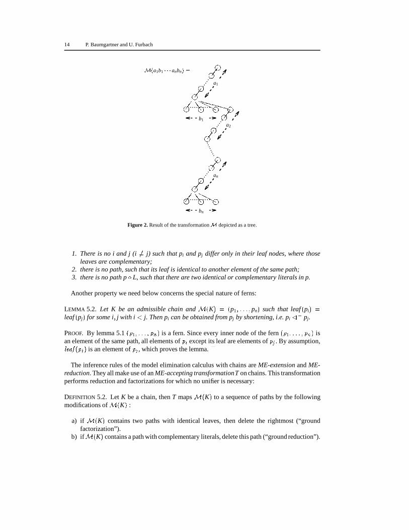
Figure 2. Result of the transformation�
depicted as a tree.
1. There is no i and j (i � j) such that pi and pj differ only in their leaf nodes, where thoseleaves are complementary;
2. there is no path, such that its leaf is identical to another element of the same path;3. there is no path p � L, such that there are two identical or complementary literals in p.
Another property we need below concerns the special nature of ferns:
LEMMA 5.2. Let K be an admissible chain and�
�K
��
�p1 � � � � � pn
�such that leaf
�pi
��
leaf
�pj
�for some i � j with i � j. Then pi can be obtained from pj by shortening, i.e. pi � � pj.
PROOF. By lemma 5.1
�� 1 � � � � � � �
�is a fern. Since every inner node of the fern
�� 1 � � � � � � �
�is
an element of the same path, all elements of � � except its leaf are elements of � � . By assumption,� � � �
�� �
�is an element of � � , which proves the lemma. �
The inference rules of the model elimination calculus with chains are ME-extension and ME-reduction. They all make use of an ME-accepting transformationT on chains. This transformationperforms reduction and factorizations for which no unifier is necessary:
DEFINITION 5.2. Let K be a chain, then T maps�
�K
�to a sequence of paths by the following
modifications of�
�K
�:
a) if�
�K
�contains two paths with identical leaves, then delete the rightmost (“ground
factorization”).b) if
��K
�contains a path with complementary literals, delete this path (“ground reduction”).

Consolution as a Framework for Comparing Calculi 15
�
In the original definition from (Loveland, 1978) there is an additional case, which allows theelimination of certain A-literals to the right of the right-most B-literal. Since we are dealing withan explicit representation of paths this is not necessary in our case. It is left as a simple exercise tothe reader to show that the transformation � as defined above for sequences of paths is identicalto the one given in Loveland’s’ calculus for chains.
The inference rules are similar to the ones of tableau model elimination, namely extension andreduction.
DEFINITION 5.3. Given a matrix M and an admissible chain K with�
�K
��
�p1 � � � � � pn
�.
The inference rule ME-extension is defined by:�p1 � � � � � pn
�� C
T
��
�
where
C is a variable disjoint (from p1 � � � � � pn) variant of a clause from M�leaf
�pn
�� L
�is a connection with MGU , where L which is the last (rightmost) literal
of the sequence � C,� ��p�1 � � � � � p�m� 1 � p�m rearrange
�T
�� C� � L�
� � �
with
�p�1 � � � � � p�m
�� T
�p1 � � � � � pn
�
and
�p�1 � � � � � p�m
�is admissible
and p�m � pn and T
�� C
�still contains L and is admissible.
The function rearrange sorts the paths of T
�� C� � L�
�, which all have length 1,
according to a given order. This will be discussed below.
The inference rule ME-reduction is defined by:�p1 � � � � � pn
�
T
�p1 � � � � � pn
�
where
there is an L in pn, such that
�L � leaf
�pn
� �is a connection with MGU .
�
We omitted an important feature of this sort of model elimination, namely the use of an orderingrule. It is explained in detail in (Loveland, 1978); for our purposes it is sufficient to note thatit determines the order of these literals, which are added to a path in an extension step. Thefunction rearrange in the ME-extension can be defined in a way which expresses the meaning ofthe ordering rule.
Analogously to the previous section, we use the notion of an ME derivation .As an example take the Matrix � � �
��
�� �
��
�� �
��
�and the two sequences of (unit-
)paths
� �� �
��
�and
� �� �
��
�. The intermediate sequence of paths � is
� �� �
� ��
� �
��
�
An application of the transformation � to this sequence deletes the rightmost path. Hence

16 P. Baumgartner and U. Furbach
we get �
��
��
� ��
�as the result of one ME-extension step. In the tableau model elimination
calculus an extension step would give � �� �
� ��
� �
��
�; the “ground factorization” performed
by the � -operation, however, can only be simulated by an additional deduction, which eliminatesthe path
�� �
�� .
THEOREM 5.1. (Sequence Consolution Simulates ME) Let M be a Matrix and
�� 1 � � � � � � s
�an
ME derivation. Then there are variants of clauses C1 � � � � � Cs� 1 from M, such that
�� 1 � � C1
� � � � �� s� 1 �� Cs � 1� � s
�is a sequence consolution derivation of M.
PROOF. In the first case let � � � 1 be derived from � � ��� 1 � � � � � � �
�by an ME-extension step with
“auxiliary chain” � � � . We construct a sequence consolvent by first multiplying path sequences:
� � � � � ��� 1 � � � � � � � � � � � � �
�
We perform the following simplification:
A) The substitution is obtained by unifying the connection
�� � � � � �
�� �
� �, which was used
in the extension step, where � is the rightmost literal of � � � .B) – From
�� � � � �
� we can delete the complementary path
�� �
��
� � to obtain�
� 1 � � � � � � � � � � � 1 � � � � � � � � � � � �
� ��
� 1 � � � � � � � � � � � 1 � � � � � � � � � � � � �
The result is depicted in figure 3.– From this path sequence we delete those paths which contain a ground connection in
the prefix � � , 1 � � � � and get:�� �1
�� � �
�� � � � � � �� � 1
�� � �
�� � ��
�� � � � � �
� �
Note, that by definition of the ME-extension rule � � does not have a connection,hence we know � �� � � � .
C) Now we shorten
- paths to obtain �� �1 � � � � � � �� � 1 � � ��
�� � � � � �
� �
- from this we shorten all � �� for which a path � �� exists with� � �
and � � � ��� ��
��
� � � ��� ��
�, such that � �� � � �� . This is possible because of lemma 5.2.
D) From the above results we delete rightmost multiple occurrences of paths, to obtain finally
�
��
�� 1 � � � � � � � � 1
��
�� � �
�� � � � � �
� � �
which is exactly the sequence �
��
�from the definition of the ME-extension rule. Note that
by the outermost application of � only paths with identical leaves are deleted, paths containingcomplementary literals are already deleted by the inner applications. These paths are alreadyeliminated by the second shortening in step C).
In the other case let � � � 1 be derived from � � ��� 1 � � � � � � �
�by an ME-reduction step. Let
� �be an arbitrary “auxiliary chain”. There is a , such that � � is complementary. As before, weconstruct a consolvent by first multiplying path sequences:
� � � � � ��� 1 � � � � � � � � � � � � �
�
From
�� 1 � � � � � � � � � � � � �
� we delete those complementary paths
�� � � � �
� , which contain

Consolution as a Framework for Comparing Calculi 17
����
��
��
��
�
����
��� � � � ������ �
��
�
��
�
����
��� � � � ������
( (L L
) � )�
pn� 1 � pn �
��
��
��
�
����
��� � � � ������
( )L
p1 �
�
. . .
Figure 3. A sequence of paths from theorem 5.1.
their connection in the prefix � � . Next we shorten paths and delete those multiple occurrencessuch that we finally obtain
�
�� 1 � � � � � �
��
�
Let us conclude this section with remarks on a comparison of model elimination and tableaumodel elimination. In tableau model elimination extension and reduction steps are possible on anypath from the tableau � . ME-extension and ME-reduction steps, however, are only possible onthe last path from � , where � is understood as a sequence of paths. Another significant differenceis that model elimination applies the T-operation, which corresponds to ground factorization andground reduction at various opportunities within one application of an inference rule. In tableaumodel elimination these steps have to be simulated by additional inference steps. It is interestingto note that consolution has a direct counterpart to the ground-reduction part of the T-operation.After applying the MGU to a path set, all complementary paths have to be deleted, which isexactly the effect of a T-operation.
6. The Connection Method
As mentioned in the introduction, consolution is intended to bridge the gap between matrixmethods, such as the connection method, and resolution. Hence, it should be possible to carryon in the spirit of the previous sections and show that consolution simulates the connectionmethod. Such a result was not established in (Eder, 1991) and will be done in this section. Asanother interesting aspect we will discuss the relation of the connection method to tableau modelelimination.
In order to do all this, one has to lay down the connection calculus. However, according to(Bibel, 1987) the connection method should not be understood as a single calculus, but as amethodology to design calculi; every calculus that proceeds by discovering a connection in everypath through a given matrix (i.e. finds a “spanning set of connections”) should be consideredas a connection method. Clearly, for our purpose we have to commit ourselves to a single such“connection calculus”. Here we will define a connection calculus that is very similar to the onein (Eder, 1992).

18 P. Baumgartner and U. Furbach
THE CONNECTION METHOD AND TABLEAU MODEL ELIMINATION
The example in section 3 can serve to illustrate the connection method in relation to tableaumodel elimination. The sequence of the trees depicted there can also be read as a connectionmethod refutation. In general the following differences have to be obeyed:
1 In selecting the next branch to be extended, only a longest branch among the collection ofopen branches may be considered. This corresponds to the stack-like search organizationin Eder’s calculus. In other words, when deleting the branches already closed, every treein a derivation then takes the form of a fern.
2 The clauses in Eder’s calculus are sets. As a consequence, identically labeled brancheshave to be collapsed into a single occurrence.
3 Eder’s calculus permits several of the new branches to be closed in one single extensionstep, i.e. several connections may be established in the step. This corresponds in tableaumodel elimination to one single extension step (with one single connection) followed by asequence of reduction steps. This correspondence will be put more precisely below. A wordof warning: the set of connections is allowed to be empty. Thus we may extend withoutclosing any branch. Such steps have no counterpart in model elimination.
4 Most importantly, with regard to the search space, a connection need not be establishedbetween a literal of the extending clause and the leaf of the extended branch, but any otherliteral in the branch will do as well. Thus the search space in this connection method ismuch broader.
These observations are reflected in the following definition.
DEFINITION 6.1. (Connection Calculus) Given a matrix M. A path is a sequence of literals. Apath set is a set of paths. The inference rule (connection) extension is defined as follows:
� � p
�� C
�where
� � p
�is a path set with longest branch p, and
C is a variable disjoint variant of a clause in M, andlet D
�C (D possibly empty) such that there is a set of connections between every literal
in D and literals in p with MGU , and� ���
�p � C� D
� �
The path p is called the selected path. Derivation is defined with respect to the single inferencerule “connection extension” as for model elimination (def. 3.2).
�
Note the differences between connection extension and extension in tableau model elimination,which mirror the above informal consideration. In particular, � is a set of several literals andthe paths resulting from the elements in � are all closed. Thus the connection calculus extensionstep can be viewed as a “macro” combination of a single tableau model elimination extensionstep, followed by some reduction steps with the remaining literals. This observation is the keyfor the stepwise simulation of tableau model elimination by the connection method. However,some precautions must be taken to achieve this goal: first, model elimination must be restricted

Consolution as a Framework for Comparing Calculi 19
to work on a longest branch. This is motivated by the longest-branch restriction of extension inthe connection method. The second point is more serious and concerns the macroscopic natureof connection extension: suppose we have executed a model elimination extension step � whichresults in the new open paths � 1 � � � � � � � . In the subsequent refutation each of these paths willeither be closed by a reduction step or will be extended to closed paths. Now, in order to enablethe stepwise simulation by a connection extension step, tableau model elimination is restricted inthe following way: if in the subsequent derivation there is an extension step on one of the paths� 1 � � � � � � � , then every reduction step on (another) of the paths � 1 � � � � � � � must be executed priorto that extension step. Such derivations will be called compact in the next definition, which startsthe formal treatment of this matter.
DEFINITION 6.2. (Compact Model Elimination Derivation) Let
�� 1 � � � � � � n
�be a model eli-
mination derivation, and suppose the selected paths are denoted by p1 � � � � � pn� 1 (in order). If theinference rule applied to some � i (i � � 1 � � � n 1
�) is an extension step, then define the set of
“new” paths brought in by that extension step as
newi :��pi � Ci � � Li �
� i
where Ci is the variant of the clause used, Li is the literal to build the connection and i is theMGU used (cf. def. 3.2).
A model elimination derivation is called compact iff whenever an extension step is applied to� i (i � � 1 � � � n 1
�) the following holds:
if some pj (n � j � i) is the selected path in a reduction step, and pj is an instanceof an occurence of a path in newi
then every selected path pk (i � k � j) is an instance of an occurence of a path innewi and is subject to a reduction step.
�
The completeness of compact tableau model elimination follows from the completeness resultin (Baumgartner, 1992) and its “independence of the computation rule”, that allows for arbitraryre-ordering of inferences in a derivation.
Note that the connection method deals with sets of sequences, whereas tableau model elimina-tion deals with multisets of sequences. Whenever required for relationships, multisets are mappedto sets in the obvious way (cf. also the similar discussion on data structures in section 4).
Building on this, we arrive at the following theorem:
THEOREM 6.1. (The Connection Method Simulates Tableau Model Elimination) Let M be amatrix and let
�� 1 � � � � � � n
�be a compact tableau model elimination derivation from M, such
that in every inference step the selected path is of maximal length. Then there exists a connectionmethod derivation
�� 1 � � � � � � k
�, for some k � n, from M and a substitution � such that � k�
�� n.
PROOF. Induction on the length � of the given derivation.Base case: If � � 1 then the model elimination derivation
�� 1
�consists of a single path set� � (a multiset of sequences) for some
� � � . Let the connection method derivation be
�� 1
�
which consists of a single path set � � (a set of sequences). When read as a set of sets it evidentlyholds that � 1 equals � 1. Hence with � :� � the claim holds.

20 P. Baumgartner and U. Furbach
Induction step: We observe that for derivations of length � 1 the given model eliminationderivation has a very special structure: first, the sequences in � 1 are all of length 1. Hence the firststep is an extension step, since no reduction step is applicable to a sequence of length 1. Second,due to this, for every compact model elimination derivation the sequence of selected paths canevidently be written as
� 01 � � 1
1 � � � � � � � 11 � �
� � � 1
� � � � � � 0� � � 1� � � � � � � � �� � �
� � � �
where precisely the � 0� (� � 1 � � � � ) are selected for an extension step, and all other �
� �� ( � � � 0)are selected for a reduction step with membership in � � � � as indicated. We will make use of thisstructure below.
By the induction hypothesis suppose the result to hold for the model elimination derivations�� 1 � � � � � � �
�(for all � � � ). Hence, a connection method derivation
�� 1 � � � � � � �
�exists with
� � � and a substitution � such that � � ��
� � . We have to show that a connection methodderivation
�� 1 � � � � � � � �
�exists with � � � � such that for some � � : � � � � �
�� � . In order to do so,
we have to trace back to the most recent extension step, and assemble this step and all subsequentreduction steps to a single connection method extension step. More formally, according to theabove consideration about the structure of compact model elimination derivations, the sequenceof selected paths in the given model elimination derivation is
� 01 � � 1
1 � � � � � � � 11 � � � � � � 0� � � 1� � � � � � �
� ��
where � 0� is the selected path in the most recent model elimination extension step, all subsequent
steps are reduction steps, and �� �� is the selected path in � � � 1. Note that if � � � 0 then � � � 1 is
obtained by a model elimination extension step, otherwise by a model elimination reduction step.Suppose
� � is the variant of the clause used in the model elimination extension step of � 0� ,which can be partitioned as
� 0� � � � 0� � � 0��
(6.1)
and 0 is the MGU used. Hence � � � � ��� 0� � � � � � � �
� 0 where � � is the literal in
� � that buildsthe connection. Since the model elimination derivation is compact, all subsequent reduction stepsremove instances of paths in � � � � from the path set. More precisely, in the reduction step where� �� (
� � � 1 � � � � ��) is the selected path and � is the MGU used, a path in � � � � 0 1 � is
removed from � �� . Now let
� �� :� � � � � � � � �: � 0� � � 0 1 � � � � � � 0 1 � is removed in � ��
�
be those literals from� � which extend the selected path � 0� to those paths being removed in the
reduction steps. It somewhat eases argumentation to use � � :� � �� � � ��
in the sequel. Then theextension step and the subsequent reduction steps each remove exactly one instance (by MGU 0 1 � ) of an element of � 0� � � from � �� (for
� � � 0 � � � � � ��). As the result of the final
reduction step we can write with (6.1)
� � ��� � 0� � 0� � � � � � �
� 0 1 � � (6.2)
Let
�� 0
1 � � 11 � � � � � � � 1
1� � � � � � 0�
�be a prefix of the given model elimination derivation leading to
the last extension step. By the induction hypothesis there exists a (not longer than the derivationending in � 0� ) connection method derivation
�� 1 � � � � � � �
�and a substitution � with � � �
�� 0� .
We further distinguish two cases:Case 1: p0
i � � l � . In words: the model elimination derivation extends a path that is not present

Consolution as a Framework for Comparing Calculi 21
in the corresponding connection method path set. Thus with � � ��
� � 0� it follows
� � � 0 1 � ��� � 0� 0 1 � �� �� � 0�
�� 0� � � � � � �
� � 0 1 � �
� � �Hence � � and the substitution � 0 1 � � satisfies the claim for � � .
Case 2 ( case 1): p0i � � l � . We intend to simulate the model elimination extension step of� 0� and the subsequent reduction steps (if any), including the final one which led to � � , by a
single connection method extension step (figure 4). The one premise path set for the connectionmethod extension step is � � � � �� � � �
�, where the selected path � � corresponds to � 0� , i.e.
� � � � � 0� (6.3)
For the other path set recall from the definition that we have to find a variable disjoint variant�
of an input clause from � and determine a set ��
�which forms a set of connections with
the selected path � � by an MGU. In this case we take for�
the same clause as used in the lastextension step in the model elimination derivation, i.e.
�:� � � . For � we choose the literals
used to build the deleted paths , i.e. � :� � � in the connection method extension step. In orderto carry out the inference it has to be shown that by some MGU � every path in
�� � � �
�� is
complementary (by this we mean that the leaf of a path is complementary to another elementin the path). This can be shown as follows: every MGU 0 1 � renders a path in � 0� � � �complementary (
� � � 1 � � � � � � ��). Hence also the more specific substitution 0 1 � � does.
Thus every path in
�� 0� � � �
� 0 1 � � is also complementary. With (6.3) and the assumption
that � does not act upon the variables of� � (without loss of generality
� � can also be assumed tobe variable disjoint from � 0� ) it follows�
� 0� � � �� 0 1 � � �
�� � � � �
�� 0 1 � � (6.4)
Since � 0 1 � � renders every path in � � � � � complementary, there is an MGU � and a
substitution � � such that�� � � � � � � � � �
0�
1 � � � � � � � � � 0 1 � � (6.5)
Using � the desired connection method extension step can be carried out, yielding the path set
� � � 1 ��� ��
�� � � � � � � �
� �� (6.6)
From the induction hypothesis and (6.3) we conclude
� �� ��
� � 0� (6.7)
Now things can be put together:
� � � 1 � ��6 �6 ��
�� ��
�� � � � � � � �
� �� � �
� � �� � � � �� � � � � � � �
�� � �
�6 �5 �� � �� � 0 1 � �
�� � � � � � � �
�� � �
�By an expression of the form � �dom� we mean the restriction of � to the domain of � , i.e. from � just those
assignments to variables are selected which have also an assignment in � .

22 P. Baumgartner and U. Furbach
�6 �5 � 6 �4 �� � �� � 0 1 � �
�� 0� � � � � � �
� 0 1 � �
�6 �7 �� �
� � 0� �� 0� � � � � � �
� � 0 1 � �
�6 �2 �� � �
Hence � � � 1 and � � satisfy the claim. �
The converse of the theorem does not hold. This is due to the restriction in tableau modelelimination that in inferences the leaf of the selected path must be part of the connection.
THE CONNECTION METHOD AND SEQUENCE CONSOLUTION
Let us now relate the connection method to consolution. Note that the observation we madeduring the discussion of tableau model elimination that led to the definition of sequence conso-lution can be made with the connection calculus as well. In the connection calculus one is notforced to delete all complementary paths, whereas by Eder’s consolution one is forced to do this.
As a consequence we need sequence consolution to establish the following result:
THEOREM 6.2. (Sequence Consolution Simulates the Connection Method) Let M be a matrixand
�� 1 � � � � � � n
�a connection calculus derivation. Then variants of clauses C1 � � � � � Cn from M
exist, such that
�� 1 � � C1
� � � � � n� 1 � � Cn� 1� � n
�is a sequence consolution derivation of M.
PROOF. Let � � � 1 be derived by extension with � � , then we construct the following sequenceconsolvent:� � has the form � �� � �
�and
� � is a variant of a clause in � , hence � � and � � � do not havevariables in common. Let � �
�� � be the set of literals selected for closing. According to the
sequence consolution inference rule we then have to multiply these two to obtain � � � � � ��� �� � �
� � � � � �
�� �� � � �
�
�� � � �
�, which further has to be modified with our simplification
rule, Version 2 from definition 3.5:
A) is obtained by unifying the connection
�� � � � � �
��
� �, which was used in the extension
step.B) � � is obtained from
�� � � � �
� by deleting the paths
�� � �
� � for every � � � � from�
� � � �� ; thus � � �
� �� �� � � �
�
�� � � � � � �
� �
C,D) from � � we shorten all paths from
�� �� � � �
� and delete all duplicate occurrences to
obtain � �� which finally gives � ��� ��
�� � � � � � �
� �
Clearly � is the result of the extension step as well. �
7. Resolution Simulates Tableau Model Elimination
Up to now we know the relation of several calculi to consolution; these include resolution,tableau model elimination, Loveland’s model elimination and a connection calculus. In order tolearn more about the relationships of these calculi, we show here the relation between resolutionand tableau model elimination. More specifically, we will show that resolution stepwise simulatestableau model elimination.
To express the result, we define the multiset of open leaves of a path set � as the multiset

Consolution as a Framework for Comparing Calculi 23
���
�:� � � � � �
��
�� � � �
�. In order to compare multisets to sets, we map multisets � to sets
in the obvious way by � � :� � � � � occurs at least once in ��. Now we claim:
THEOREM 7.1. (Resolution Simulates Tableau Model Elimination) Let M be a matrix andlet
�� 1 � � � � � � n
�be a tableau model elimination derivation from M such that in every � i (i �
1 � � � n 1) a longest branch is selected. Then there exist a resolution derivation
�C1 � � � � � Ck
�,
for some k � n, from M and a substitution � such that Ck ��
O
�� n
�� .
Let us call the elements of a tableau model elimination derivation tableaux.In every tableau � � in a derivation,
��� �
�(the set of leaves of open paths) can be seen as the
goal set still to be proved. Furthermore, since the leaf of a branch selected for an inference hasto be part of the connection (cf. definition 3.2), one could say that this goal set is consecutivelyprocessed in a linear way. It is thus quite natural to relate a tableau model elimination refutationto a linear resolution refutation by relating every
��� �
�in the model elimination refutation to the
near parent in a linear resolution refutation (see e.g. (Chang and Lee, 1973) for linear resolution).This relationship is given in the theorem as the subset relation
� � ��
��� �
�� . Thus the model
elimination-tableau can be seen, modulo instantiation, as an “upper bound” for the correspondinggoal clause in resolution. In other words, the resolution goal clause subsumes the tableau modelelimination goal.
The inference rules of model elimination and resolution correspond as follows: an extensionstep corresponds to a resolution step of the goal clause with an input clause, and a reduction stepcorresponds to a resolution step of the goal clause with an ancestor clause. This will be put moreprecisely in the proof below.
The following example is typical for the simulation; it shows the mapping of data structures,the mapping of inference rules, and also where factoring comes into resolution, which is notneeded in model elimination:
� � � ��� �
��
� � � �
� � � �
�� �
��
�
� ��
� ��
� � � �
� � � �
�
�� �
��
�
� � �
� ��
� � � � � � � � � � � � � � � � � � � � � � � ��
� �� �
� � �
� ��
�
� ��
�
�1 :
�� �
� �� �
2 : �
� �� �
� �3 :
��
� ��
� � � � � � � � � � � � � � � � � � � � � � � � � � � �
� 1 : � 2 : � 3 :
The set of open nodes�
�� 1
�� of � 1 is exactly the clause
�1; the same holds for � 2 and�
2, where � 2 is obtained from � 1 by extension with �
� ��
�
� � . The interesting case is thereduction step with MGU � � � � �
�applied to obtain � 3. In general, reduction steps with
an ancestor literal � are mapped to linear resolution steps, where the far parent clause is theclause corresponding to a previously derived tableau that contains � as open leaf. In the example� �
�� � , the previously derived tableau is � 1, and the corresponding clause is
�1. However,
resolution forces the parent clauses to be variable disjoint. Hence we have to use a variant of�
1,

24 P. Baumgartner and U. Furbach
e.g.� �1 �
�� � � �
� �� � . Using an appropriate unifier we arrive at the resolvent
��
� �� of
�2
and� �1. Note that with � � � � � �
�we can find a substitution such that the theorem holds.
Here we can see where factorization comes in: suppose that e.g. a unit clause �
� were given.�
� can be used to close � 3, but if�
3 were not factorized prior to binary resolution to the clause�� , then the resolvent would be
�� and the theorem would not hold.
It turns out that the simulation cannot be done precisely step by step. One could say thatresolution is more “optimal” than model elimination in the following sense: in resolution dueto the set data structure identical literals are collapsed into one single occurrence, whereas thecorresponding data structure in tableau model elimination are multisets and thus permit multipleoccurrences of identical literals. As a consequence for derivations, in tableau model eliminationidentical subgoals have to be proven independently from each other, whereas resolution treatsthem in one step. So it is not surprising that the resolution refutation may be shorter than themodel elimination refutation. Informally, the resolution refutation has to “pause” while in thetableau model elimination refutation a subgoal is proved that is absent in the resolution clausedue to the set data structure. Note that this property of resolution has nothing to do with the useof lemmas.
We will use the following standard definition of resolution (Chang and Lee, 1973):
DEFINITION 7.1. (Resolution, (Chang and Lee, 1973)) Let C1 and C2 be clauses and � 1 and� 2 respectively be most general factorization substitutions for some subsets of C1 and C2,respectively. Let L1 � C1 and L2 � C2 such that L1� 1 and L2 � 2 are unifiable by MGU . Thenthe resolvent of C1 and C2 is the clause
�C1 � 1 � L1
�� 1
�
�C2 � 2 � L2
�� 2
��
PROOF. (theorem 7.1) Induction on � , the length of the ME derivation.Base case: If � � 1 then � 1 is a path set � � with
� � � . With � � � the result holds trivially.Induction step: Suppose by the induction hypothesis that the result holds for derivations of
length � , i.e. there is a resolution derivation for� � from � and a � such that
� � ��
��� �
�� (7.1)
We show that the claim holds also for derivations of length � �1. This is done by case analyses
with respect to the inference rule applied to � � .Case 1: an extension step applied (cf figure 5). By definition of tableau model elimination 3.2,� � � � � �
�, � � � �
��
�� �
and�
is a variant of a clause in � such that for some � � �,�
� � � �is a connection. Let be the MGU used for that connection. Then
��� � � 1
��
��
�� �
� � � � �
�
� � �� �
� (7.2)
We do a further case analysis. In the first (and trivial) case� � � � � . But then it follows
from (7.1) and (7.2)� � �
��
�� � � 1
�� . Setting � :� � proves the claim. In the second case� � � � � . Here the extension step of � � with
�has to be simulated in a resolution step of
� �with
�. As mentioned in the introductory example, a little care must be taken to factorize on
“enough” literals of the parent clauses. For the extension step it suffices to factor only� � . For
this,� � can be partitioned as
� � � � � , where � and � are disjoint and � is a maximal setsuch that � � � � �
�. Let � 1 be a most general factorization substitution for �
�� � (by this
we mean a most general substitution with domain and range as the variables of� � such that �
becomes a singleton). � 1 is more general than � . Hence there exists a substitution � 1 such that� � � 1 � 1 � � � � (7.3)

Consolution as a Framework for Comparing Calculi 25
Now consider�
. Let � 2 be the restriction of to the variables of�
. Then� � 2 � � (7.4)
Since � 1 does not introduce new variables to� � it follows that � 1, which is applied to
� � � 1,can be assumed to act on the variables of
� � only. Without loss of generality assume�
to be a“new” variant. Hence � 1 does not act upon the variables of
�. Thus also
� � � � 1. Applying � 2
to both sides yields� � 2 � � � 1 � 2 (7.5)
Since�
is a new variant, � 2 acts on the variables of�
only. It follows� � � 1 � 1 � � � � 1 � 1 � 2 (7.6)
Concerning � it follows from this, (7.3) and � � � � � �
� � 1 � 1 � 2 � � � �
(7.7)
Since is a unifier for � and�
(modulo sign) we have with (7.7), (7.5) and (7.4) that � 1 � 2 is aunifier (modulo sign) for � � 1 and � �
�. But then there is also an MGU � for � � 1 and � �
�and
a substitution � � such that� � � 1 � � � � � � � 1 � 1 � 2 and (7.8)
� � � � � � � 1 � 2 (7.9)
Hence we can resolve the factor� � � 1 of
� � with selected literal � � 1 against�
with selectedliteral � and MGU � . The resolvent
� � � 1 is the clause� � � 1 �
�� � � 1 � � � 1 �
�
�� � � �
� �
�
� � � 1 � �
� � � �� �
�
Here we have used the fact that � and � are disjoint, even after instantiation with � 1 � . Nextwe will prove that
� � � 1 is the desired clause and � � is the desired substitution, i.e.� � � 1 � �
��
�� � � 1
�� .
� � � 1 � � ��� � 1 �
�� � � �
� �
� �� �
� � � 1 � � � �
� � � �� �
�� �
�7 �8 �7 �6 �7 �3 �� � �
�� � � �
� �
�� ��
� � �
� � �� �
� � ��7 �9 �7 �5 �7 �4 �� � �
�� � �
� � � � ��
�� � � � �
� �
�� � �
� � �
7 �1 �� �
��� �
�� � � � �
�
� � �� �
�7 �2 ��
��� � � 1
��
In
��
�we used the disjointness and maximality properties of � and � as defined above.
Thus the derivation of� � � 1 and the substitution � � proves the claim.
Case 2: a reduction step applied. By definition of reduction step (def. 3.2), � � � � � �
�,
� � � ���
�� �
and � contains a literal � such that
�� � � �
is a connection. Let � � 1 be the MGUused for that connection. As a result of the reduction step we obtain
��� � � 1
��
��
�� �
� � � � �
� � 1 (7.10)
26 P. Baumgartner and U. Furbach
The literal � that is used in the reduction step must have been the leaf of a path � in apreviously derived tableau � � (for some � � � ), i.e. � � �
�� �
�. We may assume that � �
is the last tableau in the derivation that contains that occurrence of � . Thus � � � 1 is obtainedfrom � � by extending the path � . Concerning the set of open leaves we have
��� � � 1
��� �
��� �
� � �
� � �
� � 1
� � � 1, where
�� � 1 is the (possibly empty) set of open leaves stemming
from this extension step, and � � 1 is the MGU used. By the given assumption in every inferencestep a longest path is selected. As a consequence of this and the fact that every inference removesexactly the selected path, the paths eliminated in the tableaux � � � 1 � � � � � � � are all (instances of)a longest extension of q. Thus no (instance of) a path already contained in � � � �
�is removed.
Hence�
�� � � �
� �� �
�� �
� � �
�persists; more formally we have:
� � � ��
1 � � � � �1 :
��
�� �
� � �
� � � � 1 �
��
�� �
�(7.11)
Since � � � by the induction hypothesis there is a� � and a � � such that
� � � ��
��� �
�� (7.12)
Also by the induction hypothesis there is a� � and a � � such that
� � � ��
��� �
�� (7.13)
Let � (� � �
�1 � � � � ) be the MGU applied in the derivation of � � from � � � 1. Since the MGUs
are applied to the whole path set, � is instantiated to � � � 1 � in � � . Let � � 1 be the MGUused in the reduction step. Thus� � � 1 � � � � 1 � � � 1 (7.14)
In the sequel we will abbreviate � � 1 � � � 1 as � .Now we distinguish three cases. In the first (trivial) case,
� � � � � � . This is similar to thefirst trivial case in extension step, i.e.
� � and � :� � � � � 1 will do. In the second (also trivial)case � � � � � � , i.e. the clause
� � corresponding to the previous tableau � � does not contain theancestor literal. Thus
� � and the substitution � :� � � � will do.In the non-trivial case
� � � � � ��
� � � � � � . It is similar to the non-trivial case in theextension step, except that resolution of
� � with an input clause�
is replaced by resolution of� � with the ancestor clause� � . Unlike in the extension step,
� � this time has to be factorized:take e.g.
� � �� �
�� � � �
��
and � has the leaf � �� �
��. Suppose � is extended and contains
the leaf � �
��
which is subject to a reduction step with
� ��
�now. Let
� � � � �
�� �
� �
��.
After the reduction step the set of open leaves contains neither
� ��
�nor
� ��
�. Hence the
corresponding literals from the corresponding clauses have to be resolved away. Note that this ispossible only after factoring both
� ��
� � � ��
�as well as
� ��
� �
� ��
�to a singleton.� � can be partitioned as
� � � � � , where � and � are disjoint and � is a maximal set suchthat � � � � � 1 � � � � � 1
�. Let � 1 be a most general factorization substitution for �
�� � . � 1
is more general than � � � � 1. Hence there is a substitution � 1 such that� � � 1 � 1 � � � � � � � 1 (7.15)
Now consider� � . Similarly to
� � ,� � can be partitioned as
� � � � � , where � and � aredisjoint and � is a maximal set such that � � � � � � � �
�. Let � 2 be a most general factorization
substitution for � . Since � 2 is more general than � � � there is a substitution � 2 such that� � � 2 � 2 � � � � � � (7.16)
Since � 1 does not introduce new variables to� � it follows that � 1, which is applied to
� � � 1,can be assumed to act on the variables of
� � only. Without loss of generality assume� � to be a

Consolution as a Framework for Comparing Calculi 27
“new” variant, variable disjoint from� � . Hence � 1 does not act upon the variables of
� � . Thusalso
� � � 2 � � � � 2 � 1. Applying � 2 to both sides yields� � � 2 � 2 � � � � 2 � 1 � 2 (7.17)
Concerning � it follows from this equation, (7.16) and � � � � � � � ��
� � 2 � 1 � 2 � � � ��
(7.18)
Since� � is a new variant and � 2 does not introduce new variables, � 2 acts on the variables of� � only. It follows
� � � 1 � 1 � � � � 1 � 1 � 2 (7.19)
Concerning � it follows from this equation, (7.15) and � � � � � 1 � � � � � 1
�
� � 1 � 1 � 2 � � � � � 1
�(7.20)
Since � � 1 is a unifier for � � � 1 � and�
(modulo sign) we have with (7.18) and (7.20)that � 1 � 2 is a unifier (modulo sign) for � � 1 and � � 2. But then there is also an MGU � for � � 1
and � � 2 and a substitution � � such that� � � 1 � � � � � � � 1 � 1 � 2 and (7.21)� � � 2 � � � � � � � 2 � 1 � 2 (7.22)
Hence we can resolve the factor� � � 1 of
� � with selected literal � � 1 against the factor� � � 2 of� � with selected literal � � 2 and MGU � . The resolvent
� � � 1 is the clause� � � 1 �
�� � � 1 � � � 1 �
�
�� � � 2 � � � 2 �
�
� � � 1 � � � 2 �Here we have used the fact that � and � (or � and � respectively) are disjoint, even afterinstantiation with � 1 � (or � 2 � ). Next we will prove that
� � � 1 is the desired clause and � � is thedesired substitution, i.e.
� � � 1 � ��
��� � � 1
�� .
� � � 1 � � ��� � 1 � � � 2 �
�� �
� � � 1 � � � � � 2 � � ��7 �21 �7 �19 � 7 �15 �� � � � � � 1 � � 2 � � �
�7 �22 �7 �17 � 7 �16 �� � � � � � 1 � � � �
� � ���
� � � � � � 1 � � � � 1
� � � � � �
� � � ���
� � � � � � 1 � � � � 1
� �
�� � � � � � � �
� ��7 �12 � 7 �13 �
� ��
�� �
�� � � � �
� � 1 ��
�� �
�� � �
� ��
�7 �10 �� �
��� � � 1
�
��
�� �
� � �
� ��
��
�7 �11 �� �
�� � � 1
��
In
��
�we used the disjointness and maximality properties of � and � as defined above. The
same holds in
�� �
�for � and � .
Thus the derivation of� � � 1 and the substitution � � proves the claim. �
In (Eder, 1992) Eder gives a theorem that relates the connection calculus to resolution. This

28 P. Baumgartner and U. Furbach
theorem is also relevant for tableau model elimination, since tableau model elimination can beseen as a restricted variant of the connection method. In fact, the theorem can easily be adapted totableau model elimination. Then it states, similarly to our theorem above, that for every tableaumodel elimination refutation there is a resolution refutation that is no longer. However there aresome differences: firstly, his proof is informal, whereas we feel the need for a rigorous formaltreatment. Using our notation, he states that either
��� �
�� subsumes
� � or else an input clausesubsumes
� � . Note that we do not need the input clause set and thus have a tighter coupling ofthe refutations. Furthermore note that we use the converse subsumption relation, i.e. we claimthat
� � subsumes�
�� �
�� . It might seem obvious then to conclude that
� � and�
�� �
�� are
equivalent. However this is not true since Eder uses a different resolution calculus from the onewe do: we use Chang and Lee’s definition, where factorization is carried out on the parent clauses.Eder treats factorization by an extra inference rule and thus can even factor resolvents; but moreimportant than the order of factoring is the fact that for Eder’s proof the factorization inferencerule has to be replaced by a subsumption inference rule. His subsumption rule however works ina highly non-standard way: it allows the derivation of a clause � from a clause
�if
�subsumes
� . Note that this rule reverses the standard subsumption rule; in Eder’s calculus the clause �is obtained from
�by introducing arbitrary literals and by arbitrary instantiation. The rule is
applied in place of factorization in the traditional calculus, i.e. it is applied to the parent clausesbefore the binary resolution inference. In our view, this is a counter-intuitive inference rule thatalso destroys the idea of simulating extension steps by resolution steps.Using Eder’s resolution it might be possible to prove the theorem the way we stated it (althoughwe did not check it). However it is not possible to show Eder’s subsumption relation with ourcalculus.
8. Discussion
RESUMEE
One starting point for this work was Eder’s consolution together with his investigation on itsrelation to resolution. We gave a variant of consolution, which is stronger than consolution, in thesense that every consolution derivation can be simulated stepwise by this variant. This sequenceconsolution was used as a framework for comparing other calculi. For this we presented thecalculi under consideration in the language of consolution, i.e. using paths and sets or sequencesof paths. For the sake of completeness we cite from (Eder, 1991) the following theorem, whichrelates resolution and consolution:
THEOREM 8.1. (Eder, 1991)(Consolution Simulates Resolution) Let Mbe a matrix and
�C0 � � � � �Cn
�
be a resolution refutation of M. Then
�� C1
� � � � � � Cn
�is a consolution refutation of M.
Together with the results from this paper we arrive at the diagram in figure 6. There, � � �means that calculus � can be simulated stepwise by calculus � , and dashed arrows indicate a“weaker” simulatability relation after certain calculus restrictions.
Although our main concern was to demonstrate the advantages of sequence consolution forthese investigations, we obtained several new results and formal proofs of folklore-like theorems.

Consolution as a Framework for Comparing Calculi 29
RELATION TO OTHER WORK
In (Letz, 1993) the “clausal tableau calculus” is chosen as a starting point for a comparisonof various calculi and proof procedures. It corresponds exactly to Beth’s or Smullyan’s analytictableaux calculus (Beth, 1959; Smullyan, 1968) when restricted to propositional formulas whichare given in clause form. This calculus can be further restricted, such that tableau expansions areallowed only when the clause used for the extension step introduces at least one complementaryliteral compared with the leaf choosen for extension. This calculus is exactly our tableau modelelimination calculus; it is called “connection tableau calculus” in (Letz, 1993). However, thistaxonomy is not so straightforward when first order calculi are compared. In this case, there isa significant difference, in that analytic tableaux use an instantiation rule, whereas the tableaumodel elimination calculus needs unification; this is the reason why, at least in the first order case,the tableau model elimination resembles very much the model elimination calculus introducedby Loveland in (Loveland, 1968).Another interesting property discussed by Letz is proof-confluence. The tableau calculus forexample is proof-confluent, because any tableau can be completed to a closed one if the input setis unsatisfiable, whereas tableau model elimination is not proof-confluent; i.e. a proof procedurebased on the latter has to perform some kind of backtracking.
In (Wrightson, 1989) the relation of analytic tableaux to various calculi and strategies isdiscussed. Wrightson gives in his paper a transformation of some sample resolution and modelelimination proofs into proofs using clausal tableaux. His work addresses very much the sameproblems as our work does; whereas Wrightson gives a number of example deductions togetherwith transformations, our main concern was to present rigorous theorems, stating how somecalculi can be related to each other. For example, Wrightson transforms one resolution refutationfor a propositional formula into an analytic tableaux proof; the resolution proof is a linear inputrefutation and to us it is not clear if and how this approach works for non-linear resolution proofsas well.
Bibel gave a comparative study of several proof procedures in (Bibel, 1982). There, a numberof proof procedures are compared with three versions of the connection method (which werecalled “matrix methods” at that time). Bibel gave a theorem which establishes a relation betweenthe “pure model elimination” (PME) calculus and the connection method. This PME calculuscorresponds to our tableau model elimination and hence our theorem 5.1 is a proof of Bibel’stheorem by means of the consolution-framework. It is obvious that a similar one-to-one simulationfor Loveland’s model elimination is not possible. We are confident that our approach, usingsequence consolution as a framework calculus, helps to understand the common ground and thedifferences between those calculi.
In (Loveland, 1972), the relation between ME and several other calculi is investigated. Asa main result, which is also contained and proved in a similar form in (Loveland, 1978), itdemonstrated that ME and a certain restriction of linear resolution simulate each other by steps atthe ground level. On the non-ground level ME may require additional extension steps that do nothave a counterpart in resolution. This is shown by means of an example, and this example canalso be used to show the same negative result for tableau model elimination. Also in that paper thelinked conjunct procedure and a matrix reduction procedure (Prawitz, 1970) are discussed, and itis demonstrated at the ground level that under certain circumstances there is a 1-to-1 relationshipbetween matrix reduction and ME.
Plaisted (Plaisted, 1990) has obtained a mapping (on the ground level) from model eliminationto a sequent calculus (see e.g. (Gallier, 1987)). Using this setting he shows that it suffices to applyreduction steps to leaves with one (say: negative) polarity only.

30 P. Baumgartner and U. Furbach
ON COMPLEXITY
Let us finally make some remarks on complexity results. All results of this paper depicted infigure 6 state a stepwise or shorter – and hence p(olynomial) – simulatability relation betweencalculi. There are a lot of interesting problems when one tries to establish simulatability indirections opposite to those shown in figure 6 by giving up stepwise simulatability. In (Eder,1992) it is shown that the connection calculus simulates resolution only exponentially withrespect to proof length. With the same argumentation we can conclude that the tableau modelelimination calculus exponentially simulates resolution.
Negative results with respect to stepwise simulatabilityare also contained in (Schreiber, 1974).He relates an early presentation of the connection method according to Bibel and two variantsof the resolution calculus (binary resolution with factoring and linear resolution). By means ofexamples he shows several relationships between Bibel’s method and the two resolution variants.
In (Letz, 1993) it is proven that the tableau model elimination calculus (in this paper calledconnection tableau as mentioned above) cannot polynomially simulate clausal tableaux. Since theconnection calculus can be understood as a clausal tableau calculus with a special path-selectionfunction, that result fits into our scenario. Letz further investigated the difference between regularversions of calculi, i.e. where multiple occurences of a literal within one path are forbidden.Among others, it then turns out that regular tableau model elimination cannot polynomiallysimulate (non-regular) tableau model elimination.
The importance of regularity and its detection in derivations is another argument for introducingsequence consolution. Recall that sequence consolution does not merge occurrences of the sameliterals along a path (as consolution does). Hence regularity, or the violation of regularity, can bedetected easily.
ACKNOWLEDGEMENTS
Thanks to Elmar Eder and Don Loveland for commenting on previous versions of this work.Three anonymous referees gave many valuable hints for improvement.
References
Baumgartner, P. (1992). A Model Elimination Calculus with Built-inTheories. In Ohlbach, H.-J.,editor, Proceedings of the 16-th German AI-Conference (GWAI-92), pages 30–42. Springer.LNAI 671.
Baumgartner, P., Furbach, U., and Petermann, U. (1992). A Unified Approach to Theory Reaso-ning. Forschungsbericht 15/92, University of Koblenz. (submitted to Journal of AutomatedReasoning).
Beth, E. (1959). The Foundations of Mathematics. Noth Holland.Bibel, W. (1982). A Comparative Study of Several Proof Procedures. Artificial Intelligence,
18:269–293.Bibel, W. (1987). Automated Theorem Proving. Vieweg, 2nd edition.Chang, C. and Lee, R. (1973). Symbolic Logic and Mechanical Theorem Proving. Academic
Press.Eder, E. (1991). Consolution and its Relation with Resolution. In Proc. IJCAI ’91.Eder, E. (1992). Relative Complexities of First Order Languages. Vieweg.Fitting, M. (1990). First Order Logic and Automated Theorem Proving. Texts and Monographs
in Computer Science. Springer.

Consolution as a Framework for Comparing Calculi 31
Gallier, J. (1987). Logic for Computer Science: Foundations of Automatic Theorem Proving.Wiley.
Letz, R. (1993). First-Order Proof Calculi and Proof Procedures for Automated Deduction. PhDthesis, Technische Hochschule Darmstadt.
Letz, R., Schumann, J., Bayerl, S., and Bibel, W. (1992). SETHEO: A High-Performace TheoremProver. Journal of Automated Reasoning, 8(2).
Loveland, D. (1968). Mechanical Theorem Proving by Model Elimination. JACM, 15(2).Loveland, D. (1969). A Simplified Version for the Model Elimination Theorem Proving Proce-
dure. JACM, 16(3).Loveland, D. (1972). A Unifying View of Some Linear Herbrand Procedures. JACM, 19(2).Loveland, D. (1978). Automated Theorem Proving - A Logical Basis. North Holland.Plaisted, D. (1990). A Sequent-Style Model Elimination Strategy and a Positive Refinement.
Journal of Automated Reasoning, 4(6):389–402.Prawitz, D. (1970). A Proof Procedure with Matrix Reduction. In Symposium on Automatic
Demonstration, pages 207–214. Springer. Lecture Notes in Mathematics 125.Schreiber, J. (1974). Vergleichende qualitative and quantitative Untersuchungen von Beweisver-
fahren. Technical Report 7411, Techn. Universitat Munchen, Abteilung Mathematik.Smullyan, R. (1968). First Order Logic. Springer.Stickel, M. (1988). A Prolog Technology Theorem Prover: Implementation by an Extended
Prolog Compiler. Journal of Automated Reasoning, 4:353–380.Stickel, M. (1989). A Prolog Technology Theorem Prover: A New Exposition and Implementation
in Prolog. Technical note 464, SRI International.Wrightson, G. (1989). Resolution and Analytical Tableaux. A Mapping. Technical Report
UNARP–89–4, University of Newcastle, Australia.
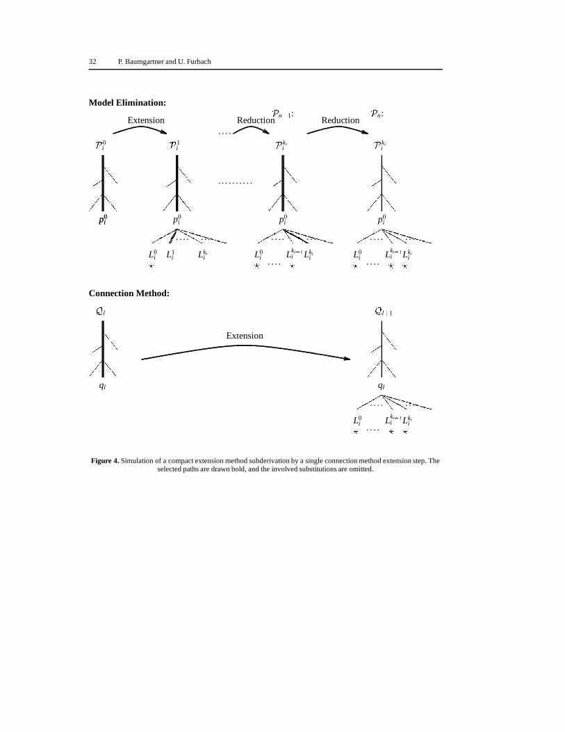
32 P. Baumgartner and U. Furbach
���� � � � � � �
��
��
��
��
��� � �
L0i Lki
i�
p0i
� kii
Lki � 1i� �
� n:
���� � � � � � �
��
��
��
��
��� � �
L0i Lki
i� Lki � 1i� �
� l� 1
ql
���� � �� � � � � � �
��
��
��
��
���� � � � � � �
��
��
��
��
���� � � ��� � � ��� � � �
��
��
��
��
��
��
��
��
L0i L1
i Lkii�
p0i
� 1i
L0i Lki
i�
p0i
� kii
Lki � 1i�
Extension� n� 1:
Reduction
� l
ql
Extension
Model Elimination:
Connection Method:
Reduction
� 0i
p0ip0i
Figure 4. Simulation of a compact extension method subderivation by a single connection method extension step. Theselected paths are drawn bold, and the involved substitutions are omitted.

Consolution as a Framework for Comparing Calculi 33
L
(by induction)
���
��
���
��
��
��
��
�
���
��
���
���
��
�
��
�
� � � � �
p p
K K
L
C �
Model Elimination:
Resolution:
KCk � � �
C �Ck �
L
D E E� 1
� 1 � Ck� 1
(with � � )
Extension with
FactorResolution
� n : � n� 1 :
�
D� 1
Figure 5. Simulating a model elimination extension step.
� � � � � � � � � � � � � �
�������������
����
����
����4.2
4.1
Resolution
7.1 6.1
Connection
Sequence Consolution
Tableau-Model-Elimination
Loveland’sModel-Elimination
Calculus
Consolution
8.1 3.16.2
5.1
Figure 6. Theorems of this paper.
Copyright © 2022 FDOKUMEN