Intersection typesfor the resource control lambda calculi

S. Ghilezan1,⋆, J. Ivetic1,⋆ , P. Lescanne2, S. Likavec3,⋆

1 University of Novi Sad, Faculty of Technical Sciences, Serbiagsilvia@uns.ac.rs jelenaivetic@uns.ac.rs

2 University of Lyon, Ecole Normal Superieure de Lyon, Francepierre.lescanne@ens-lyon.fr

3 Dipartimento di Informatica, Universita di Torino, Italylikavec@di.unito.it

Abstract. We propose intersection type assignment systems for two resourcecontrol term calculi: the lambda calculus and the sequent lambda calculus withexplicit operators for weakening and contraction. These resource control calculi,λr and λGtz

r , respectively, capture the computational content of intuitionistic nat-ural deduction and intuitionistic sequent logic with explicit structural rules. Ourmain contribution is the characterisation of strong normalisation of reductions inboth calculi. We first prove that typability implies strong normalisation in λr byadapting the reducibility method. Then we prove that typability implies strongnormalisation in λGtz

r by using a combination of well-orders and a suitable em-bedding of λGtz

r -terms into λr-terms which preserves types and enables the sim-ulation of all its reductions by the operational semantics of the λr-calculus. Fi-nally, we prove that strong normalisation implies typability in both systems usinghead subject expansion.

Introduction

It is well known that simply typed λ-calculus captures the computational content ofintuitionistic natural deduction through Curry-Howard correspondence [21]. This con-nection between logic and computation can be extended to other calculi and logicalsystems [19]: Parigot’s λµ-calculus [28] corresponds to classical natural deduction,whereas in the realm of sequent calculus, Herbelin’s λ-calculus [20], Espırito Santo’sλGtz-calculus [14], Barbanera and Berardi’s symmetric calculus [3] and Curien and Her-belin’s λµµ-calculus [11] correspond to its intuitionistic and classical versions. Extend-ing λ-calculus (λGtz-calculus) with explicit operators for weakening and contractionbrings the same correspondence to intuitionistic natural deduction (intuitionistic se-quent calculus) with explicit structural rules, as investigated in [22, 23, 18].

Among many extensions of the simple type discipline is the one with intersec-tion types, originally introduced in [9, 10, 29, 33] in order to characterise terminationproperties of term calculi [36, 16, 17]. The extension of Curry-Howard correspondenceto other formalisms brought the need for intersection types into many different set-tings [13, 24–26].⋆ Partially supported by the Ministry of Education and Science of Serbia, projects III44006 and ON174026

Our work is inspired by Kesner and Lengrand’s work on resource operators for λ-calculus [22]. Their linear λlxr calculus introduces operators for substitution, erasureand duplication, preserving at the same time strong normalisation, confluence and sub-ject reduction property of its predecessor λx [8].

Explicit control of erasure and duplication leads to decomposing of reduction stepsinto more atomic steps, thus revealing the details of computation which are usually leftimplicit. Since erasing and duplicating of (sub)terms essentially changes the structureof a program, it is important to see how this mechanism really works and to be able tocontrol this part of computation. We choose a direct approach to term calculi, namelylambda calculus and sequent lambda calculus, rather than taking a more common paththrough linear logic [1, 7]. In practice, for instance in the description of compilers byrules with binders [31, 32], the implementation of substitutions of linear variables byinlining is simple and efficient when substitution of duplicated variables requires thecumbersome and time consuming mechanism of pointers and it is therefore importantto tightly control duplication. On the other hand, precise control of erasing does notrequire a garbage collector and prevents memory leaking.

We introduce the intersection types into λr and λGtzr , λ-calculus and λGtz-calculus

with explicit rules for weakening and contraction. To the best of our knowledge, this isa first treatment of intersection types in the presence of resource control operators. Ourintersection type assignment systems λr∩ and λGtz

r ∩ integrate intersection into logicalrules, thus preserving syntax-directedness of the system. We assign restricted form ofintersection types, namely strict types, therefore minimizing the need for pre-order ontypes. Using these intersection type assignment systems we prove that terms in bothcalculi enjoy the strong normalisation property if and only if they are typable.

We first prove that typability implies strong normalisation in λr-calculus by adapt-ing the reducibility method for explicit resource control operators. Then we prove strongnormalisation for λGtz

r by using a combination of well-orders and a suitable embeddingof λGtz

r -terms into λr-terms which preserves types and enables the simulation of allits reductions by the operational semantics of the λr-calculus. Finally, we prove thatstrong normalisation implies typability in both systems using head subject expansion.

The paper is organised as follows. In Section 1 we extend the λ-calculus and λGtz-calculus with explicit operators for weakening and contraction obtaining λr-calculusand λGtz

r -calculus, respectively. Intersection type assignment systems with strict typesare introduced to these calculi in Section 2. In Section 3 we first prove that typabilityimplies strong normalization in λr-calculus by adapting the reducibility method. Thenwe prove that typability implies strong normalization in λGtz

r -calculus by using a com-bination of well-orders and a suitable embedding of λGtz

r -terms into λr-terms whichpreserves types and enables the simulation of all its reductions by the operational se-mantics of the λr-calculus. Section 4 gives a proof of strong normalization of typableterms for both calculi using head subject expansion. We conclude in Section 5.

1 Untyped resource control calculi

1.1 Resource control lambda calculus λr

The resource control lambda calculus, λr, is an extension of the λ-calculus with ex-plicit operators for weakening and contraction. It corresponds to the λcw-calculus ofKesner and Renaud, proposed in [23] as a vertex of ”the prismoid of resources”.

The pre-terms of λr-calculus are given by the following abstract syntax:

Pre-terms f ::= x |λx. f | f f |x⊙ f |x <x1x2 f

where x ranges over a denumerable set of term variables. λx. f is an abstraction, f f is anapplication, x⊙ f is a weakening and x <x1

x2 f is a contraction. The contraction operatoris assumed to be insensitive to order of the arguments x1 and x2 i.e. x <x1

x2 f = x <x2x1 f .

The set of free variables of a pre-term f , denoted by Fv( f ), is defined as follows:Fv(x) = x; Fv(λx. f ) = Fv( f )\{x}; Fv( f g) = Fv( f )∪Fv(g);Fv(x⊙ f ) = {x}∪Fv( f ); Fv(x <x1

x2 f ) = {x}∪Fv( f )\{x1,x2}.In x <x1

x2 f , the contraction binds the variables x1 and x2 and a free variable x isintroduced. The operator x⊙ f also introduces a free variable x. In order to avoid paren-theses, we let the scope of all binders extend to the right as much as possible.

The set of λr-terms, denoted by Λr and ranged over by M,N,P,M1, .... is a subsetof the set of pre-terms, defined in Figure 1.

x ∈ Λr

f ∈ Λr x ∈ Fv( f )

λx. f ∈ Λr

f ∈ Λr g ∈ Λr Fv( f )∩Fv(g) = /0f g ∈ Λr

f ∈ Λr x /∈ Fv( f )x⊙ f ∈ Λr

f ∈ Λr x1,x2 ∈ Fv( f ) x /∈ Fv( f )

x <x1x2 f ∈ Λr

Fig. 1. Λr: λr-terms

Informally, we say that a term is a pre-term in which in every subterm every freevariable occurs exactly once, and every binder binds (exactly one occurrence of) a freevariable. This notion corresponds to the notion of linear terms in [22]. In that sense,only linear expressions are in the focus of our investigation. This assumption is not arestriction, since every non linear λ-term has its linear correspondent, as illustrated bythe following example.

Example 1. Pre-terms λx.y and λx.xx are not λr-terms, on the other hand pre-termsλx.(x⊙ y) and λx.x <x1

x2 (x1x2) are λr-terms.In the sequel, we use the notation X ⊙M for x1 ⊙ ... xn ⊙M and X <Y

Z M for x1 <y1z1

... xn <ynzn M, where X , Y and Z are lists of the size n, consisting of all distinct variables

x1, ...,xn,y1, ...,yn,z1, ...,zn.

(β) (λx.M)N → M[N/x]

(γ1) x <x1x2 (λy.M) → λy.x <x1

x2 M (ω1) λx.(y⊙M) → y⊙ (λx.M), x = y(γ2) x <x1

x2 (MN) → (x <x1x2 M)N, if x1,x2 ∈ Fv(M) (ω2) (x⊙M)N → x⊙ (MN)

(γ3) x <x1x2 (MN) → M(x <x1

x2 N), if x1,x2 ∈ Fv(N) (ω3) M(x⊙N) → x⊙ (MN)

(γω1) x <x1x2 (y⊙M) → y⊙ (x <x1

x2 M), y = x1,x2 (γω2) x <x1x2 (x1 ⊙M) → M[x/x2]

Fig. 2. Reduction rules of λr-calculus

The reduction rules of λr-calculus are presented in Figure 2.The inductive definition of the meta operator [ / ], representing the substitution of

free variables, is given in Figure 3. In this definition, the terms N1 and N2 are obtainedfrom N by renaming of all the free variables in N by fresh variables.

x[N/x] , N (y⊙M)[N/x] , y⊙M[N/x], x = y(λy.M)[N/x] , λy.M[N/x], x = y (x⊙M)[N/x] , Fv(N)⊙M(MP)[N/x] , M[N/x]P, x ∈ Fv(M) (y <y1

y2 M)[N/x] , y <y1y2 M[N/x], x = y

(MP)[N/x] , MP[N/x], x ∈ Fv(P) (x <x1x2 M)[N/x] , Fv(N)<

Fv(N1)Fv(N2)

M[N1/x1][N2/x2]

Fig. 3. Substitution in λr-calculus

In the λr, one works modulo equivalencies given in Figure 4.

x⊙ (y⊙M) ≡ y⊙ (x⊙M) x <x1x2 M ≡ x <x2

x1 Mx <y

z (y <uv M) ≡ x <y

u (y <zv M) x <x1

x2 (y <y1y2 M) ≡ y <y1

y2 (x <x1x2 M), x = y1,y2, y = x1,x2

M[(y⊙N)/x] ≡ y⊙M[N/x] M[(y <y1y2 N)/x] ≡ y <y1

y2 M[N/x], y1,y2 ∈ Fv(N)

Fig. 4. Equivalences in λr-calculus

1.2 Resource control sequent lambda calculus λGtzr

The resource control lambda Gentzen calculus λGtzr is derived from the λGtz-calculus

(more precisely its confluent sub-calculus λGtzV ) by adding the explicit operators for

weakening and contraction. It is proposed in [18]. The abstract syntax of λGtzr pre-

expressions is the following:

Pre-values F ::= x |λx. f |x⊙ f |x <x1x2 f

Pre-terms f ::= F | f cPre-contexts c ::= x. f | f :: c |x⊙ c |x <x1

x2 c

where x ranges over a denumerable set of term variables.

A pre-value can be a variable, an abstraction, a weakening or a contraction; a pre-term is either a value or a cut (an application). A pre-context is one of the following:a selection, a context constructor (usually called cons), a weakening on pre-contextor a contraction on a pre-context. Pre-terms and pre-contexts are together referred toas the pre-expressions and will be ranged over by E. Pre-contexts x⊙ c and x <x1

x2 cbehave exactly like corresponding pre-terms x⊙ f and x <x1

x2 f in the untyped calculus,so they will not be treated separately. The set of free variables of a pre-expression isdefined analogously to the free variables in λr-calculus with the following additions:

Fv( f c) = Fv( f )∪Fv(c); Fv(x. f ) = Fv( f )\{x}; Fv( f :: c) = Fv( f )∪Fv(c).Like in the case of λr-calculus, the set of λGtz

r -expressions (namely values, termsand contexts), denoted by ΛGtz

r ∪ΛGtzr,C, is a subset of the set of pre-expressions, defined

as in Figure 1 plus:

f ∈ ΛGtzr x ∈ Fv( f )

x. f ∈ ΛGtzr,C

f ∈ ΛGtzr c ∈ ΛGtz

r,C Fv( f )∩Fv(c) = /0

f :: c ∈ ΛGtzr,C

Values are denoted by T, terms by t,u,v..., contexts by k,k′, ... and expressions by e,e′.The computation over the set of λGtz

r -expressions reflects the cut-elimination pro-cess. Four groups of reductions in λGtz

r -calculus are given in Figure 5.

(β) (λx.t)(u :: k) → u(x.tk) (σ) T (x.v) → v[T/x](π) (tk)k′ → t(k@k′) (µ) x.xk → k

(γ1) x <x1x2 (λy.t) → λy.x <x1

x2 t (ω1) λx.(y⊙ t) → y⊙ (λx.t), x = y(γ2) x <x1

x2 (tk) → (x <x1x2 t)k, if x1,x2 ∈ Fv(t) (ω2) (x⊙ t)k → x⊙ (tk)

(γ3) x <x1x2 (tk) → t(x <x1

x2 k), if x1,x2 ∈ Fv(k) (ω3) t(x⊙ k) → x⊙ (tk)(γ4) x <x1

x2 (y.t) → y.(x <x1x2 t) (ω4) x.(y⊙ t) → y⊙ (x.t), x = y

(γ5) x <x1x2 (t :: k) → (x <x1

x2 t) :: k, if x1,x2 ∈ Fv(t) (ω5) (x⊙ t) :: k → x⊙ (t :: k)(γ6) x <x1

x2 (t :: k) → t :: (x <x1x2 k), if x1,x2 ∈ Fv(k) (ω6) t :: (x⊙ k) → x⊙ (t :: k)

(γω1) x <x1x2 (y⊙ e) → y⊙ (x <x1

x2 e) x1 = y = x2 (γω2) x <x1x2 (x1 ⊙ e) → e[x/x2]

Fig. 5. Reduction rules of λGtzr -calculus

The first group consists of β, π, σ and µ reductions from λGtz. New reductions areadded to deal with explicit contraction (γ reductions) and weakening (ω reductions). Thegroups of γ and ω reductions consist of rules that perform propagation of contractioninto the expression and extraction of weakening out of the expression. This disciplineallows us to optimize the computation by delaying the duplication of terms on the onehand, and by performing the erasure of terms as soon as possible on the other.

The meta-substitution v[T/x] is defined as in Figure 3 with the following additions:

(tk)[u/x] = t[u/x]k, x ∈ Fv(t) (tk)[u/x] = tk[u/x], x ∈ Fv(k)(y.t)[u/x] = y.t[u/x]

(t :: k)[u/x] = t[u/x] :: k, x ∈ Fv(t) (t :: k)[u/x] = t :: k[u/x], x ∈ Fv(k)

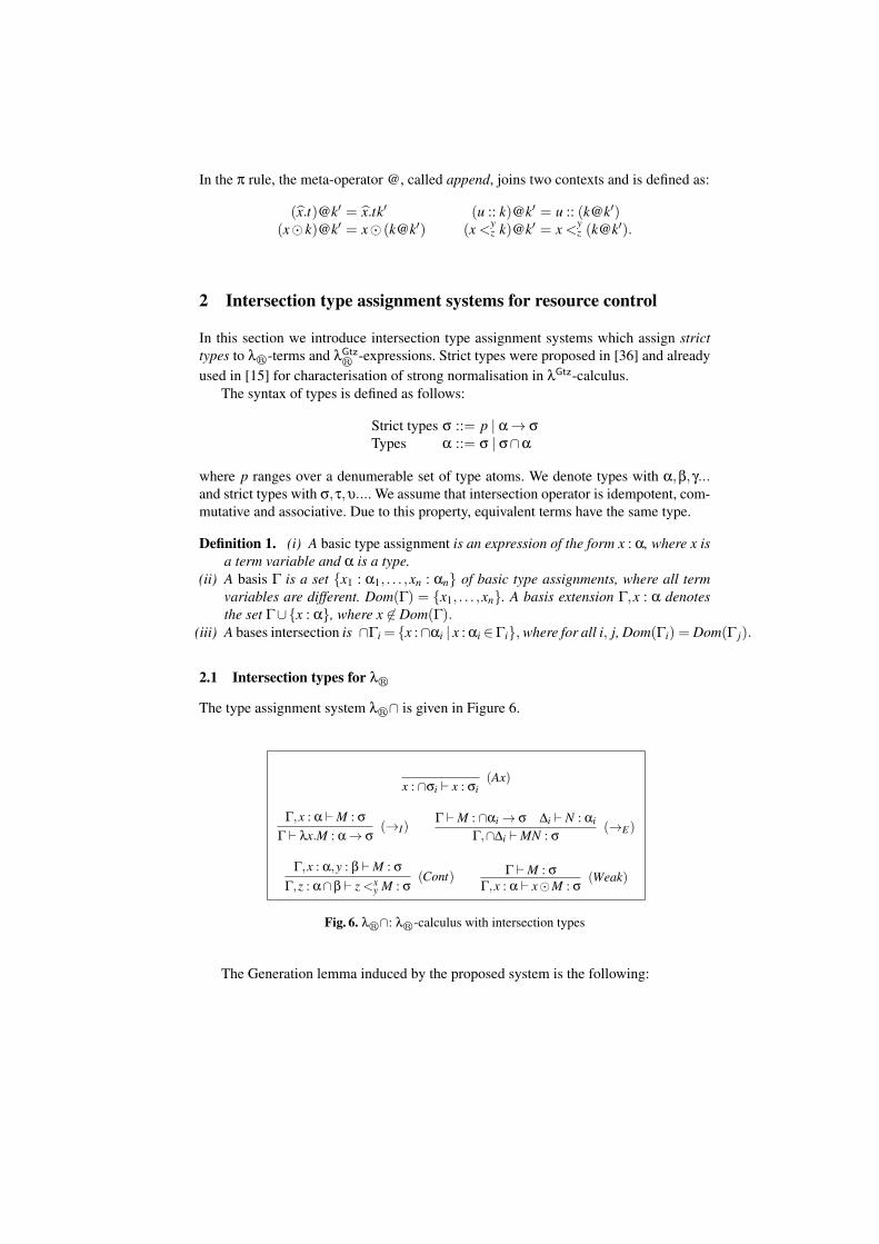
In the π rule, the meta-operator @, called append, joins two contexts and is defined as:

(x.t)@k′ = x.tk′ (u :: k)@k′ = u :: (k@k′)(x⊙ k)@k′ = x⊙ (k@k′) (x <y

z k)@k′ = x <yz (k@k′).

2 Intersection type assignment systems for resource control

In this section we introduce intersection type assignment systems which assign stricttypes to λr-terms and λGtz

r -expressions. Strict types were proposed in [36] and alreadyused in [15] for characterisation of strong normalisation in λGtz-calculus.

The syntax of types is defined as follows:

Strict types σ ::= p | α → σTypes α ::= σ | σ∩α

where p ranges over a denumerable set of type atoms. We denote types with α,β,γ...and strict types with σ,τ,υ.... We assume that intersection operator is idempotent, com-mutative and associative. Due to this property, equivalent terms have the same type.

Definition 1. (i) A basic type assignment is an expression of the form x : α, where x isa term variable and α is a type.

(ii) A basis Γ is a set {x1 : α1, . . . ,xn : αn} of basic type assignments, where all termvariables are different. Dom(Γ) = {x1, . . . ,xn}. A basis extension Γ,x : α denotesthe set Γ∪{x : α}, where x ∈ Dom(Γ).

(iii) A bases intersection is ∩Γi = {x :∩αi | x : αi ∈Γi}, where for all i, j, Dom(Γi) = Dom(Γ j).

2.1 Intersection types for λr

The type assignment system λr∩ is given in Figure 6.

x : ∩σi ⊢ x : σi(Ax)

Γ,x : α ⊢ M : σΓ ⊢ λx.M : α → σ

(→I)Γ ⊢ M : ∩αi → σ ∆i ⊢ N : αi

Γ,∩∆i ⊢ MN : σ(→E)

Γ,x : α,y : β ⊢ M : σΓ,z : α∩β ⊢ z <x

y M : σ(Cont) Γ ⊢ M : σ

Γ,x : α ⊢ x⊙M : σ(Weak)

Fig. 6. λr∩: λr-calculus with intersection types

The Generation lemma induced by the proposed system is the following:

Proposition 2 (Generation lemma for λr∩).

(i) Γ ⊢ λx.M : β iff there exist α and σ such that β ≡ α → σ and Γ,x : α ⊢ M : σ.(ii) Γ ⊢ MN : σ iff Γ = Γ′,∩∆i and there exists a type ∩αi such that

Γ′ ⊢ M : ∩αi → σ and for all i ∆i ⊢ N : αi.(iii) Γ ⊢ z <x

y M : σ iff there exist Γ′,α,β such that Γ = Γ′,z : α∩βand Γ′,x : α,y : β ⊢ M : σ.

(iv) Γ ⊢ x⊙M : σ iff there exist Γ′,β such that Γ = Γ′,x : β and Γ′ ⊢ M : σ.

The proposed system satisfies the following properties.

Proposition 3. If M → M′ then Fv(M) = Fv(M′).

Proposition 4. (i) If Γ ⊢ M : , then Dom(Γ) = Fv(M).(ii) If Γ1 ⊢ M : σ and Γ2 ⊢ M : σ , then Γ1 ∩Γ2 ⊢ M : σ .

Proposition 5 (Substitution lemma). If Γ,x : ∩αi ⊢ M : σ and for all i, ∆i ⊢ N : αi,then Γ,∩∆i ⊢ M[N/x] : σ.

Proposition 6 (Subject reduction and equivalence). For every λr-term M: if Γ ⊢ M : σand M → M′ or M ≡ M, then Γ ⊢ M′ : σ.

2.2 Intersection types for λGtzr

The type assignment system λGtzr ∩ is given in Figure 7.

x : ∩σi ⊢ x : σi(Ax)

Γ,x : α ⊢ t : σΓ ⊢ λx.t : α → σ

(→R)Γi ⊢ t : αi ∆;σ ⊢ k : τ

∩Γi,∆;∩αi → σ ⊢ t :: k : τ(→L)

Γi ⊢ t : αi ∆;∩αi ⊢ k : σ∩Γi,∆ ⊢ tk : σ

(Cut)Γ,x : α ⊢ t : σΓ;α ⊢ x.t : σ

(Sel)

Γ,x : α,y : β ⊢ t : σΓ,z : α∩β ⊢ z <x

y t : σ(Contt)

Γ ⊢ t : σΓ,x : α ⊢ x⊙ t : σ

(Weakt)

Γ,x : α,y : β;γ ⊢ k : σΓ,z : α∩β;γ ⊢ z <x

y k : σ(Contk)

Γ;γ ⊢ k : σΓ,x : α;γ ⊢ x⊙ k : σ

(Weakk)

Fig. 7. λGtzr ∩: λGtz

r -calculus with intersection types

The Generation lemma induced by the proposed system is the following:

Proposition 7 (Generation lemma for λGtzr ∩).

(i) Γ ⊢ λx.t : β iff there exist α and σ such that β ≡ α → σ and Γ,x : α ⊢ t : σ.(ii) Γ;γ ⊢ t :: k : τ iff Γ = ∩Γi,∆, γ ≡∩αi → σ, and Γi ⊢ t : αi,∀i and ∆;σ ⊢ k : τ .

(iii) Γ ⊢ tk : σ iff Γ = ∩Γi,∆ and there exists a type ∩αi such that Γi ⊢ t : αi, ∀i and∆;∩αi ⊢ k : σ.

(iv) Γ;α ⊢ x.t : σ iff Γ,x : α ⊢ t : σ.(v) Γ ⊢ z <x

y t : σ iff there exist Γ′,α,β such that Γ = Γ′,z : α∩β andΓ′,x : α,y : β ⊢ t : σ.

(vi) Γ ⊢ x⊙ t : σ iff there exist Γ′,β such that Γ = Γ′,x : β and Γ′ ⊢ t : σ.(vii) Γ;ε ⊢ z <x

y k : σ iff there exist Γ′,α,β such that Γ = Γ′,z : α∩β andΓ,x : α,y : β;ε ⊢ k : σ.

(viii) Γ;γ ⊢ x⊙ k : σ iff there exist Γ,β such that Γ = Γ′,x : β and Γ;γ ⊢ k : σ.

3 Typability ⇒ SN in both systems

3.1 Typeability ⇒ SN in λr∩

The main idea of the reducibility method, introduced in Tait [35] for proving the strongnormalization property for the simply typed lambda calculus, is to interpret types bysuitable sets of lambda terms which satisfy certain realizability properties.

In the remainder of the paper we consider Λr as the applicative structure whosedomain are λr-terms and where the application is just the application of λr-terms. Werecall some notions from [4]. The set of strongly normalizing terms is defined as

SN = {M ∈ Λr | ¬(∃M1,M2, . . . ∈ Λr)M → M1 → M2 → . . .}.

Definition 8. For M ,N ⊆ Λr, we define M // N ⊆ Λr as

M // N = {N ∈ Λr | ∀M ∈ M . ( f v(M )∩ f v(N ) = /0 ⇒ NM ∈ N )}.

Definition 9. The type interpretation [[−]] : Types → 2Λr is defined by:

(I1) [[p]] = SN , where p is a type atom;(I2) [[σ∩α]] = [[σ]]∩ [[α]];(I3) [[α → σ]] = ([[α]] // [[σ]]) = {M ∈ Λr | ∀N ∈ [[α]] MN ∈ [[σ]]}.

Next, we introduce the notions of saturation property, obtained by extending thesaturation property given in [5], and weakening property. To this aim we introduce thefollowing notation: if R denotes the set of reductions given in Figure 2, r ∈ R \ (β),then redexr (contrr) denote the left (right) hand side of the reduction r (its redex andcontractum, respectively).

Definition 10.

– A set X ⊆ SN satisfies the saturation property, notation SAT(X ), if• VAR(X ): (∀n ≥ 0) (∀x ∈ var) (∀M1, . . . ,Mn ∈ SN )

(x∩ f v(M1)∩ . . .∩ f v(Mn) = /0 ⇒ xM1 . . .Mn ∈ X .

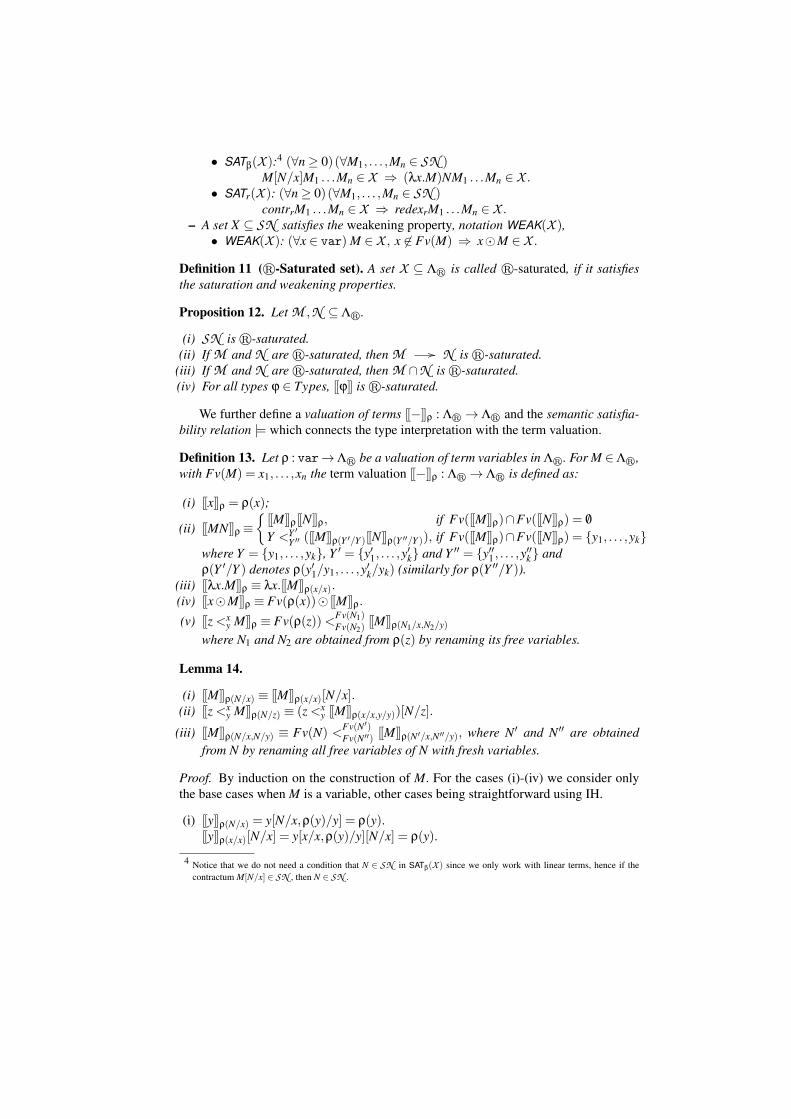
• SATβ(X ):4 (∀n ≥ 0)(∀M1, . . . ,Mn ∈ SN )M[N/x]M1 . . .Mn ∈ X ⇒ (λx.M)NM1 . . .Mn ∈ X .

• SATr(X ): (∀n ≥ 0)(∀M1, . . . ,Mn ∈ SN )contrrM1 . . .Mn ∈ X ⇒ redexrM1 . . .Mn ∈ X .

– A set X ⊆ SN satisfies the weakening property, notation WEAK(X ),• WEAK(X ): (∀x ∈ var) M ∈ X , x ∈ Fv(M) ⇒ x⊙M ∈ X .

Definition 11 (r-Saturated set). A set X ⊆ Λr is called r-saturated, if it satisfiesthe saturation and weakening properties.

Proposition 12. Let M ,N ⊆ Λr.

(i) SN is r-saturated.(ii) If M and N are r-saturated, then M // N is r-saturated.

(iii) If M and N are r-saturated, then M ∩N is r-saturated.(iv) For all types φ ∈ Types, [[φ]] is r-saturated.

We further define a valuation of terms [[−]]ρ : Λr → Λr and the semantic satisfia-bility relation |= which connects the type interpretation with the term valuation.

Definition 13. Let ρ : var→ Λr be a valuation of term variables in Λr. For M ∈ Λr,with Fv(M) = x1, . . . ,xn the term valuation [[−]]ρ : Λr → Λr is defined as:

(i) [[x]]ρ = ρ(x);

(ii) [[MN]]ρ ≡{[[M]]ρ[[N]]ρ, if Fv([[M]]ρ)∩Fv([[N]]ρ) = /0Y <Y ′

Y ′′ ([[M]]ρ(Y ′/Y )[[N]]ρ(Y ′′/Y )), if Fv([[M]]ρ)∩Fv([[N]]ρ) = {y1, . . . ,yk}where Y = {y1, . . . ,yk}, Y ′ = {y′1, . . . ,y

′k} and Y ′′ = {y′′1 , . . . ,y

′′k} and

ρ(Y ′/Y ) denotes ρ(y′1/y1, . . . ,y′k/yk) (similarly for ρ(Y ′′/Y )).(iii) [[λx.M]]ρ ≡ λx.[[M]]ρ(x/x).(iv) [[x⊙M]]ρ ≡ Fv(ρ(x))⊙ [[M]]ρ.

(v) [[z <xy M]]ρ ≡ Fv(ρ(z))<Fv(N1)

Fv(N2)[[M]]ρ(N1/x,N2/y)

where N1 and N2 are obtained from ρ(z) by renaming its free variables.

Lemma 14.

(i) [[M]]ρ(N/x) ≡ [[M]]ρ(x/x)[N/x].(ii) [[z <x

y M]]ρ(N/z) ≡ (z <xy [[M]]ρ(x/x,y/y))[N/z].

(iii) [[M]]ρ(N/x,N/y) ≡ Fv(N) <Fv(N′)Fv(N′′) [[M]]ρ(N′/x,N′′/y), where N′ and N′′ are obtained

from N by renaming all free variables of N with fresh variables.

Proof. By induction on the construction of M. For the cases (i)-(iv) we consider onlythe base cases when M is a variable, other cases being straightforward using IH.

(i) [[y]]ρ(N/x) = y[N/x,ρ(y)/y] = ρ(y).[[y]]ρ(x/x)[N/x] = y[x/x,ρ(y)/y][N/x] = ρ(y).

4 Notice that we do not need a condition that N ∈ SN in SATβ(X ) since we only work with linear terms, hence if thecontractum M[N/x] ∈ SN , then N ∈ SN .

(ii) Using (i) and the definition of substitution.[[z <x

y M]]ρ(N/z) = [[z <xy M]]ρ(z/z)[N/z] = (z <x

y [[M]]ρ(x/x,y/y))[N/z] =

Fv(N)<Fv(N1)Fv(N2)

[[M]]ρ(x/x,y/y)[N1/x][N2/y] = Fv(N)<Fv(N1)Fv(N2)

[[M]]ρ(N1/x,N2/y) =

Fv(N)<Fv(N1)Fv(N2)

[[M]]ρ(x/x,y/y)[N1/x][N2/y] = (z <xy [[M]]ρ(x/x,y/y))[N/z].

(iii) By straightforward application od Definition 13.

Definition 15.(i) ρ |= M : α ⇐⇒ [[M]]ρ ∈ [[α]];

(ii) ρ |= Γ ⇐⇒ (∀(x : α) ∈ Γ) ρ(x) ∈ [[α]];(iii) Γ |= M : α ⇐⇒ (∀ρ,ρ |= Γ ⇒ ρ |= M : α).

Proposition 16 (Soundness of λr∩). If Γ ⊢ M : α, then Γ |= M : α.

Proof. By induction on the derivation of Γ ⊢ M : α. The cases (Ax) and (→I) are anal-ogous to the corresponding rules in ordinary λ calculus. We prove the statement for theremaining inference rules.

– The last rule applied is (→E), i.e., Γ ⊢ M : ∩αi → σ,∆i ⊢ N : αi ⇒ Γ,∩∆i ⊢ MN : σ.By the IH Γ |= M : ∩αi → σ and ∆i |= N : αi,∀i. Suppose that ρ |= Γ,∩∆i, thenρ |= Γ and ρ |= ∩∆i. From ρ |= Γ, using the IH we deduce that [[M]]ρ ∈ [[∩αi → σ]].From ρ |= ∩∆i, we deduce that ρ |= ∆i,∀i (since every variable x : α ∈ ∩∆i is ofthe form x : ∩αi,x : αi ∈ ∆i), hence using the IH we deduce that [[N]]ρ ∈ [[αi]],∀i.This means that [[N]]ρ ∈ ∩[[αi]]ρ = [[∩αi]]ρ. Using Definition 13(ii) we obtain that[[M]]ρ[[N]]ρ = [[MN]]ρ ∈ [[σ]].

– The last rule applied is (Weak), i.e., Γ ⊢ M : α ⇒ Γ,x : β ⊢ x⊙M : α. By the IHΓ |= M : α. Suppose that ρ |= Γ,x : β ⇔ ρ |= Γ and ρ |= x : β. From ρ |= Γ we obtain[[M]]ρ ∈ [[α]]. Using the weakening property WEAK and Definition 13(iv) we obtainFv(ρ(x))⊙ [[M]]ρ = [[x⊙M]]ρ ∈ [[α]], since Fv(ρ(x))∩Fv([[M]]ρ) = /0.

– The last rule applied is (Cont), i.e., Γ,x : α,y : β ⊢ M : γ ⇒ Γ,z : α ∩ β ⊢ z <xy

M : γ. By the IH Γ,x : α,y : β |= M : γ. Suppose that ρ |= Γ,z : α ∩ β, in orderto prove [[z <x

y M]]ρ ∈ [[γ]]. This means that ρ |= Γ and ρ |= z : α∩ β ⇔ ρ(z) ∈[[α]] and ρ(z) ∈ [[β]]. For the sake of simplicity let ρ(z) ≡ N. We define a new ρ′

such that ρ′ = ρ(N/x,N/y). Then ρ′ |= Γ,x : α,y : β since x,y ∈ Dom(Γ), N ∈[[α]] and N ∈ [[β]]. By the IH [[M]]ρ′ ∈ [[γ]]. By the definition of term valuation(Definition 13), Lemma 14(i), (ii) and (iii) and the definition of substitution weobtain [[M]]ρ′ = [[M]]ρ(N/x,N/y) = Fv(N) <

Fv(N′)Fv(N′′) [[M]]ρ(N′/x,N′′/y) = Fv(N) <

Fv(N′)Fv(N′′)

[[M]]ρ(x/x,y/y)[N′/x][N′′/y] = (z<xy [[M]]ρ(x/x,y/y)[N/z] = ([[z<x

y M]]ρ(z/z))[N/z] = [[z<xy

M]]ρ(N/z) = [[z <xy M]]ρ, since ρ(z) = N. Hence, [[z <x

y M]]ρ ∈ [[γ]]. ⊓⊔

Theorem 17 (SN for λr∩). If Γ⊢M : α, then M is strongly normalizing, i.e. M ∈ SN .

Proof. Suppose Γ⊢M : α. By Proposition 16 Γ |=M : α. According to Definition 15(iii),this means that (∀ρ |= Γ) ρ |= M : α. We can choose a particular ρ0(x) = x for allx ∈ var. By Proposition 12(iv), [[β]] is saturated for each type β, hence x = [[x]]ρ ∈ [[β]](variable condition for n= 0). Therefore, ρ0 |=Γ and we can conclude that [[M]]ρ0 ∈ [[α]].On the other hand, M = [[M]]ρ0 and [[α]]⊆ SN (Proposition 12), hence M ∈ SN . ⊓⊔

3.2 Typeability ⇒ SN in λGtzr ∩

In this section, we prove the strong normalisation property of the λGtzr -calculus with

intersection types. The termination is proved by showing that the reduction on the setΛGtzr ∪ΛGtz

r,C of the typeable λGtzr -expressions is included in a particular well-founded

relation, which we define as the lexicographic product of three well-founded componentrelations. The first one is based on the mapping of λGtz

r -expressions into λr-terms. Weshow that this mapping preserves types and that all λGtz

r -reductions can be simulated bythe reductions or identities of the λr-calculus. The other two well-founded orders arebased on the introduction of quantities designed to decrease a global measure associatedwith specific λGtz

r -expressions during the computation.

Definition 18. The mapping ⌊ ⌋ : ΛGtzr → Λr is defined together with the auxiliary

mapping ⌊ ⌋k : ΛGtzr,C → (Λr → Λr) in the following way:

⌊x⌋ = x ⌊x.t⌋k(M) = (λx.⌊t⌋)M⌊λx.t⌋ = λx.⌊t⌋ ⌊t :: k⌋k(M) = ⌊k⌋k(M⌊t⌋)⌊x⊙ t⌋ = x⊙⌊t⌋ ⌊x⊙ k⌋k(M) = x⊙⌊k⌋k(M)⌊x <y

z t⌋ = x <yz ⌊t⌋ ⌊x <y

z k⌋k(M) = x <yz ⌊k⌋k(M)

⌊tk⌋ = ⌊k⌋k(⌊t⌋)

Lemma 19. (i) Fv(t) = Fv(⌊t⌋), for t ∈ ΛGtzr .

(ii) ⌊v[t/x]⌋= ⌊v⌋[⌊t⌋/x], for v, t ∈ ΛGtzr .

We prove that the mappings ⌊ ⌋ and ⌊ ⌋k preserve types. In the sequel, the notationΛr(Γ′⊢λrα) stands for {M | M ∈ Λr & Γ′ ⊢λr M : α}.

Proposition 20 (Type preservation with ⌊ ⌋).

(i) If Γ′ ⊢ t : α, then Γ′ ⊢λr ⌊t⌋ : α.(ii) If Γ′;α ⊢ k : β, then ⌊k⌋k : Λr(Γ′′⊢λrα) → Λr(Γ′,Γ′′⊢λr β), for some Γ′′.

Proof. The proposition is proved by simultaneous induction on derivations. We distin-guish cases according to the last typing rule used.

– Cases (Ax), (→R), (Weakt) and (Contt) are easy, because the intersection type as-signment system of λr has exactly the same rules.

– Case (Sel): the derivation ends with the rule

Γ′,x : α ⊢ t : σΓ′;α ⊢ x.t : σ

(Sel)

By IH we have that Γ′,x : α ⊢λr ⌊t⌋ : σ. For any M ∈ Λr such that Γ′′ ⊢λr M : α,for some Γ′′, we have

Γ′,x : α ⊢λr ⌊t⌋ : σ(→I)

Γ′ ⊢λr λx.⌊t⌋ : α → σ Γ′′ ⊢λr M : α(→E)

Γ′,Γ′′ ⊢λr (λx.⌊t⌋)M : σ

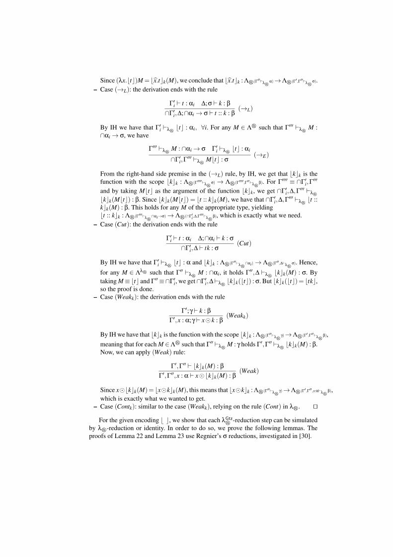
Since (λx.⌊t⌋)M = ⌊x.t⌋k(M), we conclude that ⌊x.t⌋k : Λr(Γ′′⊢λrα)→Λr(Γ′,Γ′′⊢λrσ).– Case (→L): the derivation ends with the rule

Γ′i ⊢ t : αi ∆;σ ⊢ k : β

∩Γ′i,∆;∩αi → σ ⊢ t :: k : β

(→L)

By IH we have that Γ′i ⊢λr ⌊t⌋ : αi, ∀i. For any M ∈ Λr such that Γ′′′ ⊢λr M :

∩αi → σ, we have

Γ′′′ ⊢λr M : ∩αi → σ Γ′i ⊢λr ⌊t⌋ : αi

∩Γ′i,Γ′′′ ⊢λr M⌊t⌋ : σ

(→E)

From the right-hand side premise in the (→L) rule, by IH, we get that ⌊k⌋k is thefunction with the scope ⌊k⌋k : Λr(Γ′′′′⊢λrσ) → Λr(Γ′′′′,Γ′′⊢λr β). For Γ′′′′ ≡ ∩Γ′

i,Γ′′′

and by taking M⌊t⌋ as the argument of the function ⌊k⌋k, we get ∩Γ′i,∆,Γ′′′ ⊢λr

⌊k⌋k(M⌊t⌋) : β. Since ⌊k⌋k(M⌊t⌋) = ⌊t :: k⌋k(M), we have that ∩Γ′i,∆,Γ′′′ ⊢λr ⌊t ::

k⌋k(M) : β. This holds for any M of the appropriate type, yielding⌊t :: k⌋k : Λr(Γ′′′⊢λr∩αi→σ) → Λr(∩Γ′i,∆,Γ

′′′⊢λr β), which is exactly what we need.– Case (Cut): the derivation ends with the rule

Γ′i ⊢ t : αi ∆;∩αi ⊢ k : σ

∩Γ′i,∆ ⊢ tk : σ

(Cut)

By IH we have that Γ′i ⊢λr ⌊t⌋ : α and ⌊k⌋k : Λr(Γ′′⊢λr∩αi) → Λr(Γ′′,∆⊢λrσ). Hence,

for any M ∈ Λλr such that Γ′′ ⊢λr M : ∩αi, it holds Γ′′,∆ ⊢λr ⌊k⌋k(M) : σ. Bytaking M ≡⌊t⌋ and Γ′′ ≡∩Γ′

i, we get ∩Γ′i,∆⊢λr ⌊k⌋k(⌊t⌋) : σ. But ⌊k⌋k(⌊t⌋)= ⌊tk⌋,

so the proof is done.– Case (Weakk): the derivation ends with the rule

Γ′;γ ⊢ k : βΓ′,x : α;γ ⊢ x⊙ k : β

(Weakk)

By IH we have that ⌊k⌋k is the function with the scope ⌊k⌋k : Λr(Γ′′⊢λr γ)→Λr(Γ′,Γ′′⊢λr β),meaning that for each M ∈Λr such that Γ′′ ⊢λr M : γ holds Γ′,Γ′′ ⊢λr ⌊k⌋k(M) : β.Now, we can apply (Weak) rule:

Γ′,Γ′′ ⊢ ⌊k⌋k(M) : βΓ′,Γ′′,x : α ⊢ x⊙⌊k⌋k(M) : β

(Weak)

Since x⊙⌊k⌋k(M)= ⌊x⊙k⌋k(M), this means that ⌊x⊙k⌋k : Λr(Γ′′⊢λr γ)→Λr(Γ′,Γ′′ ,x:α⊢λr β),which is exactly what we wanted to get.

– Case (Contk): similar to the case (Weakk), relying on the rule (Cont) in λr. ⊓⊔

For the given encoding ⌊ ⌋, we show that each λGtzr -reduction step can be simulated

by λr-reduction or identity. In order to do so, we prove the following lemmas. Theproofs of Lemma 22 and Lemma 23 use Regnier’s σ reductions, investigated in [30].

Lemma 21. If M →λr M′, then ⌊k⌋k(M)→λr ⌊k⌋k(M′).

Lemma 22. ⌊k⌋k((λx.P)N)→λr (λx.⌊k⌋k(P))N.

Lemma 23. If M ∈ Λr and k,k′ ∈ ΛGtzr,C, then ⌊k′⌋k ◦⌊k⌋k(M)→λr ⌊k@k′⌋k(M).

Lemma 24. (i) If x /∈ Fv(k), then (⌊k⌋k(M))[N/x] = ⌊k⌋k(M[N/x]).(ii) If x,y /∈ Fv(k), then z <x

y (⌊k⌋k(M))→λr ⌊k⌋k(z <xy M).

(iii) ⌊k⌋k(x⊙M)→λr x⊙⌊k⌋k(M).

Now we can prove that the reduction rules of λGtzr can be simulated by the reduction

rules or identities in λr-calculus.

Theorem 25 (Simulation of λGtzr -reduction by λr-reduction).

(i) If term M → M′, then ⌊M⌋ →λr ⌊M′⌋.(ii) If context k → k′ by γ6 or ω6 reduction, then ⌊k⌋k(M)≡ ⌊k′⌋k(M), for any M ∈ Λr.

(iii) If context k → k′ by some other reduction, then ⌊k⌋k(M) →λr ⌊k′⌋k(M), for anyM ∈ Λr.

The previous proposition shows that each λGtzr -reduction step is interpreted either by

a λr-reduction or by an identity. If one wants to prove that there is no infinite sequenceof λGtz

r -reductions one has to prove that there cannot exist an infinite sequence of λGtzr -

reductions which are all interpreted as identities. To prove this, one shows that if aterm is reduced with such a λGtz

r -reduction, it is reduced for another order that forbidsinfinite decreasing chains. This order is itself composed of several orders, free of infinitedecreasing chains (Definition 29).

Definition 26. The functions S , || ||C, || ||W : (ΛGtzr ∪ Λr)→N are defined in Figure 8.

S(x) = 1 ||x||C = 0 ||x||W = 1S(λx.t) = 1+S(t) ||λx.t||C = ||t||C ||λx.t||W = 1+ ||t||W

S(x⊙ e) = 1+S(e) ||x⊙ e||C = ||e||C ||x⊙ e||W = 0S(x <y

z e) = 1+S(e) ||x <yz e||C = ||e||C +S(e) ||x <y

z e||W = 1+ ||e||WS(tk) = S(t)+S(k) ||tk||C = ||t||C + ||k||C ||tk||W = 1+ ||t||W + ||k||W

S(x.t) = 1+S(t) ||x.t||C = ||t||C ||x.t||W = 1+ ||t||WS(t :: k) = S(t)+S(k) ||t :: k||C = ||t||C + ||k||C ||t :: k||W = 1+ ||t||W + ||k||W

Fig. 8. Definitions of S(e), ||e||C, ||e||W

Lemma 27. For all e,e′ : Λr:

(i) If e →γ6 e′, then ||e||C > ||e′||C.(ii) If e →ω6 e′, then ||e||C = ||e′||C.

Lemma 28. For all e,e′ ∈ Λr: If e →ω6 e′, then ||e||W > ||e′||W .

Now we can define the following orders based on the previously introduced map-ping and norms.

Definition 29. We define the following strict orders and equivalencies on ΛGtzr ∩:

(i) t >λr t ′ iff ⌊t⌋ →+λr

⌊t ′⌋; t =λr t ′ iff ⌊t⌋ ≡ ⌊t ′⌋;

k >λr k′ iff ⌊k⌋k(M)→+λr

⌊k′⌋(M) for every λr term M ;k =λr k′ iff ⌊k⌋k(M)≡ ⌊k′⌋k(M) for every λr term M;

(ii) e >c e′ iff ||e||C > ||e′||C; e =c e′ iff ||e||C = ||e′||C;(iii) e >w e′ iff ||e||W > ||e′||W ; e =w e′ iff ||e||W = ||e′||W ;

A lexicographic product of two orders >1 and >2 is usually defined as follows ([2]):a >1 ×lex >2 b ⇔ a >1 b or (a =1 b and a >2 b).

Definition 30. We define the relation ≫ on ΛGtzr as the lexicographic product:

≫ = >λr ×lex >c ×lex >w .

The following propositions proves that the reduction relation on the set of typedλGtzr -expressions is included in the given lexicographic product ≫.

Proposition 31. For each e ∈ ΛGtzr : if e → e′, then e ≫ e′.

Proof. The proof is by case analysis on the kind of reduction and the structure of ≫.If e → e′ by β, σ, π, µ, γ1, γ2, γ3, γ4 γ5, γω1, γω2, ω1, ω2, ω3 ω4 or ω5 reduction, thene >λr e′ by Proposition 25.If e → e′ by γ6, then e =λr e′ by Proposition 25, and e >c e′ by Lemma 27.Finally, if e → e′ by ω6, then e =λr e′ by Proposition 25, e =c e′ by Lemma 27 ande >w e′ by Lemma 28. ⊓⊔

SN of → is another terminology for the well-foundness of the relation → and it iswell-known that a relation included in a well-founded relation is well-founded and thatthe lexicographic product of well-founded relations is well-founded.

Theorem 32 (Strong normalization). Each expression in ΛGtzr ∩ is SN.

Proof. The reduction → is well-founded on ΛGtzr ∩ as it is included (Proposition 31) in

the relation ≫ which is well-founded as the lexicographic product of the well-foundedrelations >λr , >c and >w. Relation >λr is based on the interpretation ⌊ ⌋ : ΛGtz

r →Λr.By Proposition 20 typeability is preserved by the interpretation ⌊ ⌋ and →λr is SN (i.e.,well-founded) on Λr∩ (Section 3.1), hence >λr is well-founded on ΛGtz

r ∩. Similarly,>c and >w are well-founded, as they are based on interpretations into the well-foundedrelation > on the set N of natural numbers. ⊓⊔

4 SN ⇒ Typability in both systems

4.1 SN ⇒ Typability in λr∩

We want to prove that if a λr-term is SN, then it is typable in the system λr∩. Weproceed in two steps: 1) we show that all λr-normal forms are typable and 2) we proveThe head subject expansion property. First, let us observe the structure of the λr-normalforms, given by the following abstract syntax:

Mn f ::= x |λx.Mn f |λx.x⊙Mn f |xM1n f . . .M

nn f |x <

x1x2 Mn f Nn f , if x1 ∈ Fv(Mn f ),x2 ∈ Fv(Nn f )

Wn f ::= x⊙Mn f |x⊙Wn f

Proposition 33. λr-normal forms are typable in the system λr∩.

Proposition 34 (Inverse substitution lemma). Let Γ ⊢ M[N/x] : α and N typable.Then, there are ∆i and βi, i ∈ I such that ∆i ⊢ N : βi, ∀i and Γ′,x : ∩βi ⊢ M : α, whereΓ = Γ′,∩∆i.

Proof. By induction on the structure of M. ⊓⊔

Proposition 35 (Head subject expansion). For every λr-term M: if M → M′, M iscontracted redex and Γ ⊢ M′ : α , then Γ ⊢ M : α, provided that if M ≡ (λx.N)P →βN[P/x]≡ M′, P is typable.

Proof. By the case study according to the applied reduction. ⊓⊔

Theorem 36 (SN ⇒ typability). All strongly normalising λr-terms are typable in theλr∩ system.

Proof. The proof is by induction on the length of the longest reduction path out of astrongly normalising term M, with a subinduction on the size of M.

– If M is a normal form, then M is typable by Proposition 33.– If M is itself a redex, let M′ be the term obtained by contracting the redex M.

M′ is also strongly normalising, hence by IH it is typable. Then M is typable, byProposition 35. Notice that, if M ≡ (λx.N)P →β N[P/x] ≡ M′, then, by IH, P istypable, since the length of the longest reduction path out of P is smaller than thatof M, and the size of P is smaller than the size of M.

– Next, suppose that M is not itself a redex nor a normal form. Then M is of one of thefollowing forms: λx.N, λx.x⊙N, xM1 . . .Mn, x⊙N, or x <x1

x2 NP, x1 ∈ Fv(N), x2 ∈Fv(P) (where M1, . . . ,Mn, and NP are not normal forms). M1, . . . ,Mn and NP aretypable by IH, as subterms of M. Then, it is easy to build the typing for M. Forinstance, let us consider the case x <x1

x2 NP with x1 ∈ Fv(N), x2 ∈ Fv(P). By in-duction NP is typable, hence N is typable with say Γ,x1 : β ⊢ N : ∩αi → σ andP is typable with say ∆i,x2 : γi ⊢ P : αi. Then using the rule (E →) we obtainΓ,∩∆i,x1 : β,x2 : ∩γi ⊢ NP : σ. Finally, the rule (Cont) yields Γ,∩∆i,x : β∩(∩γi) ⊢x <x1

x2 NP : σ. ⊓⊔

4.2 SN ⇒ Typability in λGtzr ∩

Finally, we want to prove that if a λGtzr -term is SN, then it is typable in the system

λGtzr ∩. We follow the procedure used in Section 4.1. The proofs are similar to the ones

in Section 4.1 and omitted due to the lack of space.The abstract syntax of λGtz

r -normal forms is the following:tn f ::= x |λx.tn f |λx.x⊙ tn f |x(tn f :: kn f ) |x <y

z y(tn f :: kn f )kn f ::= x.tn f | x.x⊙ tn f | tn f :: kn f |x <y

z (tn f :: kn f ), y ∈ Fv(tn f ),z ∈ Fv(kn f )wn f ::= x⊙ en f |x⊙wn f

We use en f for any λGtzr -expression in the normal form.

Proposition 37. λGtzr -normal forms are typable in the system λGtz

r ∩.

The following two lemmas explain the behavior of the meta operators [ / ] and @ duringexpansion.

Lemma 38 (Inverse substitution lemma).

(i) Let Γ ⊢ t[u/x] : α and u typable. Then, there exist ∩∆i and ∩βi, i ∈ I such that∆i ⊢ u : βi, ∀i and Γ′,x : ∩βi ⊢ t : α, where Γ = Γ′,∩∆i.

(ii) Let Γ;γ ⊢ k[u/x] : α and u typable. Then, there exist ∩∆i and ∩βi, i ∈ I such that∆i ⊢ u : βi, ∀i and Γ′,x : ∩βi;γ ⊢ k : α, where Γ = Γ′,∩∆i.

Lemma 39 (Inverse append lemma). If Γ;α ⊢ k@k′ : σ, then Γ = Γ′,Γ′′ and there isa type ∩βi such that Γ′;α ⊢ k : βi, ∀i and Γ′′;∩βi ⊢ k′ : σ.

Now we prove that the type of a term is preserved during the expansion.

Proposition 40 (Head subject expansion). For every λGtzr -term t: if t → t ′, t is con-

tracted redex and Γ ⊢ t ′ : α , then Γ ⊢ t : α.

Theorem 41 (SN ⇒ typability). All strongly normalising λGtzr terms are typable in the

λGtzr ∩ system.

5 Conclusions

In this paper, we have proposed intersection type assignment systems for λr-calculus(λCW of [23]) and λGtz

r -calculus of [18]. The two intersection type systems proposedhere, for resource control lambda and sequent lambda calculus, give a complete char-acterisation of strongly normalising terms for both calculi. The strong normalisationof typeable resource lambda terms is proved directly by appropriate modification ofthe reducibility method, whereas the same property for resource sequent lambda termsis proved by well-founded lexicographic order based on suitable embedding into theformer calculus. Although the obtained results are not surprising, this paper expandsthe range of the intersection type techniques and combines different methods in thestrict types environment. Unlike the approach of introducing non-idempotent intersec-tion into the calculus with some kind of resource management [27], our intersection is

idempotent. As a consequence, our type assignment system corresponds to full intu-itionistic logic, while non-idempotent intersection type assignment systems correspondto intuitionistic linear logic.

Resource control lambda and sequent lambda calculi are good candidates to inves-tigate the computational content of substructural logics ([34]) both in natural deductionand sequent calculus. The motivation for these logics comes from philosophy (Rele-vant Logics), linguistics (Lambek Calculus) to computing (Linear Logic). The basicidea of resource control is to explicitly handle structural rules, so the absence of (some)structural rules in substructural logics such as weakening, contraction, commutativity,associativity can possibly be handled by resource control operators, which is in the do-main of further research. Another direction will involve the investigation of the use ofintersection types, being a powerful means for building models of lambda calculus ([6,12]), in constructing models for sequent lambda calculi.

Acknowledgements: We would like to thank the anonymous referees for carefulreading and many valuable comments, which helped us improve the final version of thepaper. We would also like to thank Dragisa Zunic for participating in the earlier stagesof the work.

References

1. S. Abramsky. Computational interpretations of linear logic. Theor. Comput Sci.,111(1&2):3–57, 1993.

2. F. Baader and T. Nipkow. Term Rewriting and All That. Cambridge University Press, UK,1998.

3. F. Barbanera and S. Berardi. A symmetric lambda calculus for classical program extraction.Inform. Comput., 125(2):103–117, 1996.

4. H. P. Barendregt. The Lambda Calculus: its Syntax and Semantics. North-Holland, Amster-dam, revised edition, 1984.

5. H. P. Barendregt. Lambda calculi with types. In S. Abramsky, D. M. Gabbay, and T. S. E.Maibaum, editors, Handbook of Logic in Computer Science, pages 117–309. Oxford Univer-sity Press, UK, 1992.

6. H. P. Barendregt, M. Coppo, and M. Dezani-Ciancaglini. A filter lambda model and thecompleteness of type assignment. J. Symb. Logic, 48(4):931–940 (1984), 1983.

7. N. Benton, G. Bierman, V. de Paiva, and M. Hyland. A term calculus for intuitionistic linearlogic. In 1st International Conference on Typed Lambda Calculus, TLCA ’93, volume 664of LNCS, pages 75–90. Springer, 1993.

8. R. Bloo and K. H. Rose. Preservation of strong normalisation in named lambda calculi withexplicit substitution and garbage collection. In Computer Science in the Netherlands, CSN’95, pages 62–72, 1995.

9. M. Coppo and M. Dezani-Ciancaglini. A new type-assignment for lambda terms. Archiv furMathematische Logik, 19:139–156, 1978.

10. M. Coppo and M. Dezani-Ciancaglini. An extension of the basic functionality theory for theλ-calculus. Notre Dame J. Formal Logic, 21(4):685–693, 1980.

11. P.-L. Curien and H. Herbelin. The duality of computation. In 5th International Conferenceon Functional Programming, ICFP’00, pages 233–243. ACM Press, 2000.

12. M. Dezani-Ciancaglini, S. Ghilezan, and S. Likavec. Behavioural Inverse Limit Models.Theor. Comput Sci., 316(1–3):49–74, 2004.

13. D. J. Dougherty, S. Ghilezan, and P. Lescanne. Characterizing strong normalization in theCurien-Herbelin symmetric lambda calculus: extending the Coppo-Dezani heritage. Theor.Comput Sci., 398:114–128, 2008.

14. J. Espırito Santo. Completing Herbelin’s programme. In S. R. D. Rocca, editor, 9th Interna-tional Conference on Typed Lambda Calculi and Applications, TLCA ’07, volume 4583 ofLNCS, pages 118–132. Springer, 2007.

15. J. Espırito Santo, J. Ivetic, and S. Likavec. Characterising strongly normalising intuitionisticterms. Fundamenta Informaticae, 2011. to appear.

16. J. Gallier. Typing untyped λ-terms, or reducibility strikes again! Ann. Pure Appl. Logic,91:231–270, 1998.

17. S. Ghilezan. Strong normalization and typability with intersection types. Notre Dame J.Formal Logic, 37(1):44–52, 1996.

18. S. Ghilezan, J. Ivetic, P. Lescanne, and D. Zunic. Intuitionistic sequent-style calculus withexplicit structural rules. In 8th International Tbilisi Symposium on Language, Logic andComputation, volume 6618 of LNAI, pages 101–124, 2011.

19. S. Ghilezan and S. Likavec. Computational interpretations of logics. In Z. Ognjanovic,editor, Collection of Papers, special issue Logic in Computer Science 20(12), pages 159–215. Mathematical Institute of Serbian Academy of Sciences and Arts, 2009.

20. H. Herbelin. A lambda calculus structure isomorphic to Gentzen-style sequent calculusstructure. In L. Pacholski and J. Tiuryn, editors, Computer Science Logic, CSL ’94, volume933 of LNCS, pages 61–75. Springer, 1995.

21. W. A. Howard. The formulas-as-types notion of construction. In J. P. Seldin and J. R. Hind-ley, editors, To H. B. Curry: Essays on Combinatory Logic, Lambda Calculus and Formalism,pages 479–490. Academic Press, London, 1980.

22. D. Kesner and S. Lengrand. Resource operators for lambda-calculus. Inform. Comput.,205(4):419–473, 2007.

23. D. Kesner and F. Renaud. The prismoid of resources. In R. K. c and D. Niwinski, editors,34th International Symposium on Mathematical Foundations of Computer Science, MFCS’09, volume 5734 of LNCS, pages 464–476. Springer, 2009.

24. K. Kikuchi. Simple proofs of characterizing strong normalisation for explicit substitutioncalculi. In F. Baader, editor, 18th International Conference on Term Rewriting and Applica-tions, RTA’07, volume 4533 of LNCS, pages 257–272. Springer, 2007.

25. R. Matthes. Characterizing strongly normalizing terms of a λ-calculus with generalizedapplications via intersection types. In J. R. et al., editor, ICALP Workshops 2000. CarletonScientific, 2000.

26. P. M. Neergaard. Theoretical pearls: A bargain for intersection types: a simple strong nor-malization proof. J. Funct. Program., 15(5):669–677, 2005.

27. M. Pagani and S. R. D. Rocca. Solvability in resource lambda-calculus. In C.-H. L. Ong, ed-itor, 13th International Conference on Foundations of Software Science and ComputationalStructures, FOSSACS 2010, volume 6014 of LNCS, pages 358–373. Springer, 2010.

28. M. Parigot. Lambda-mu-calculus: An algorithmic interpretation of classical natural deduc-tion. In A. Voronkov, editor, 3rd International Conference on Logic Programming and Au-tomated Reasoning, LPAR ’92, volume 624 of LNCS, pages 190–201. Springer, 1992.

29. G. Pottinger. A type assignment for the strongly normalizable λ-terms. In J. P. Seldin andJ. R. Hindley, editors, To H. B. Curry: Essays on Combinatory Logic, Lambda Calculus andFormalism, pages 561–577. Academic Press, London, 1980.

30. L. Regnier. Une equivalence sur les lambda-termes. Theor. Comput Sci., 126(2):281–292,1994.

31. K. H. Rose. CRSX - Combinatory Reduction Systems with Extensions. In M. Schmidt-Schauß, editor, 22nd International Conference on Rewriting Techniques and Applications,

RTA’11, volume 10 of Leibniz International Proceedings in Informatics (LIPIcs), pages 81–90. Schloss Dagstuhl–Leibniz-Zentrum fuer Informatik, 2011.

32. K. H. Rose. Implementation Tricks That Make CRSX Tick. Talk at IFIP 1.6 workshop,RDP’2011, May 2011.

33. P. Salle. Une extension de la theorie des types en lambda-calcul. In G. Ausiello and C. Bohm,editors, 5th International Conference on Automata, Languages and Programming, ICALP’78, volume 62 of LNCS, pages 398–410. Springer, 1978.

34. P. Schroeder-Heister and K. Dosen. Substructural Logics. Oxford University Press, UK,1993.

35. W. W. Tait. Intensional interpretations of functionals of finite type I. J. Symb. Logic, 32:198–212, 1967.

36. S. van Bakel. Complete restrictions of the intersection type discipline. Theor. Comput Sci.,102(1):135–163, 1992.