Supereulerian graphs, hamiltonicity of graphs and several ...
Upload
khangminh22Category
view
4download
0
XX
Knowledge Graphs
AIDAN HOGAN, DCC, Universidad de Chile; IMFD, Chile
EVA BLOMQVIST, Linköping University, Sweden
MICHAEL COCHEZ, Vrije Universiteit and Discovery Lab, Elsevier, The Netherlands
CLAUDIA D’AMATO, University of Bari, Italy
GERARD DE MELO, Rutgers University, USACLAUDIO GUTIERREZ, DCC, Universidad de Chile; IMFD, Chile
SABRINA KIRRANE,WU Vienna, Austria
JOSÉ EMILIO LABRA GAYO, Universidad de Oviedo, Spain
ROBERTO NAVIGLI, Sapienza University of Rome, Italy
SEBASTIAN NEUMAIER,WU Vienna, Austria
AXEL-CYRILLE NGONGA NGOMO, DICE, Universität Paderborn, Germany
AXEL POLLERES,WU Vienna, Austria
SABBIR M. RASHID, Tetherless World Constellation, Rensselaer Polytechnic Institute, USA
ANISA RULA, University of Milano-Bicocca, Italy and University of Bonn, Germany
LUKAS SCHMELZEISEN, Universität Stuttgart, Germany
JUAN SEQUEDA, data.world, USASTEFFEN STAAB, Universität Stuttgart, Germany and University of Southampton, UK
ANTOINE ZIMMERMANN, École des mines de Saint-Étienne, France
In this paper we provide a comprehensive introduction to knowledge graphs, which have recently garnered
significant attention from both industry and academia in scenarios that require exploiting diverse, dynamic,
large-scale collections of data. After some opening remarks, we motivate and contrast various graph-based
data models, as well as languages used to query and validate knowledge graphs. We explain how knowledge
can be represented and extracted using a combination of deductive and inductive techniques. We conclude
with high-level future research directions for knowledge graphs.
CCS Concepts: • Information systems→Graph-based database models; Information integration; • Com-puting methodologies→ Artificial intelligence;
Additional Key Words and Phrases: knowledge graphs, graph databases, graph query langauges, shapes,
ontologies, graph algorithms, embeddings, graph neural networks, rule mining
Authors’ addresses: Aidan Hogan, DCC, Universidad de Chile; IMFD, Chile, [email protected]; Eva Blomqvist, Linköping
University, Sweden; Michael Cochez, Vrije Universiteit and Discovery Lab, Elsevier, The Netherlands; Claudia d’Amato,
University of Bari, Italy; Gerard de Melo, Rutgers University, USA; Claudio Gutierrez, DCC, Universidad de Chile; IMFD,
Chile; Sabrina Kirrane, WU Vienna, Austria; José Emilio Labra Gayo, Universidad de Oviedo, Spain; Roberto Navigli, Sapienza
University of Rome, Italy; Sebastian Neumaier, WU Vienna, Austria; Axel-Cyrille Ngonga Ngomo, DICE, Universität Pader-
born, Germany; Axel Polleres, WU Vienna, Austria; Sabbir M. Rashid, Tetherless World Constellation, Rensselaer Polytechnic
Institute, USA; Anisa Rula, University of Milano-Bicocca, Italy, University of Bonn, Germany; Lukas Schmelzeisen, Uni-
versität Stuttgart, Germany; Juan Sequeda, data.world, USA; Steffen Staab, Universität Stuttgart, Germany, University of
Southampton, UK; Antoine Zimmermann, École des mines de Saint-Étienne, France.
Permission to make digital or hard copies of part or all of this work for personal or classroom use is granted without fee
provided that copies are not made or distributed for profit or commercial advantage and that copies bear this notice and
the full citation on the first page. Copyrights for third-party components of this work must be honored. For all other uses,
contact the owner/author(s).
© 2021 Copyright held by the owner/author(s).
0360-0300/2021/03-ARTXX
https://doi.org/0000001.0000001
ACM Comput. Surv., Vol. X, No. X, Article XX. Publication date: March 2021.

ACM Reference Format:Aidan Hogan, Eva Blomqvist, Michael Cochez, Claudia d’Amato, Gerard de Melo, Claudio Gutierrez, Sab-
rina Kirrane, José Emilio Labra Gayo, Roberto Navigli, Sebastian Neumaier, Axel-Cyrille Ngonga Ngomo,
Axel Polleres, Sabbir M. Rashid, Anisa Rula, Lukas Schmelzeisen, Juan Sequeda, Steffen Staab, and An-
toine Zimmermann. 2021. Knowledge Graphs. ACM Comput. Surv. X, X, Article XX (March 2021), 35 pages.
https://doi.org/0000001.0000001
1 INTRODUCTIONThough the phrase “knowledge graph” has been used in the literature since at least 1972 [117], the
modern incarnation of the phrase stems from the 2012 announcement of the Google Knowledge
Graph [121], followed by further announcements of knowledge graphs by Airbnb, Amazon, eBay,
Facebook, IBM, LinkedIn, Microsoft, Uber, and more besides [56, 94]. The growing industrial uptake
of the concept proved difficult for academia to ignore, with more and more scientific literature
being published on knowledge graphs [32, 76, 99, 104, 105, 139, 143].
Knowledge graphs use a graph-based data model to capture knowledge in application scenarios
that involve integrating, managing and extracting value from diverse sources of data at large
scale [94]. Employing a graph-based abstraction of knowledge has a number of benefits when
compared with a relational model or NoSQL alternatives. Graphs provide a concise and intuitive
abstraction for a variety of domains, where edges and paths capture different, potentially complex
relations between the entities of a domain [6]. Graphs allow maintainers to postpone the definition
of a schema, allowing the data to evolve in a more flexible manner [4]. Graph query languages
support not only standard relational operators (joins, unions, projections, etc.), but also navigational
operators for finding entities connected through arbitrary-length paths [4]. Ontologies [18, 52, 88]
and rules [58, 69] can be used to define and reason about the semantics of the terms used in
the graph. Scalable frameworks for graph analytics [79, 125, 147] can be leveraged for computing
centrality, clustering, summarisation, etc., in order to gain insights about the domain being described.
Promising techniques are now emerging for applying machine learning over graphs [139, 144].
1.1 Overview and NoveltyThe goal of this tutorial paper is to motivate and give a comprehensive introduction to knowledge
graphs, to describe their foundational data models and how they can be queried and validated, and
to discuss deductive and inductive ways to make knowledge explicit. Our focus is on introducing
key concepts and techniques, rather than specific implementations, optimisations, tools or systems.
A number of related surveys, books, etc., have been published relating to knowledge graphs. In
Table 1, we provide an overview of the tertiary literature – surveys, books, tutorials, etc. – relating
to knowledge graphs, comparing the topics covered to those specifically covered in this paper.
We see that the existing literature tends to focus on particular topics shown. Some of the related
literature provides more details on particular topics than this paper; we will often refer to these
works for further reading. Unlike these works, our goal as a tutorial paper is to provide a broad
and accessible introduction to knowledge graphs. In the final row of the table, we indicate the
topics covered in this paper ( ✓ ) and an extended version ( E ) published online [56]. While this
paper focuses on the core of knowledge graphs, the extended online version further discusses
knowledge graph creation, enrichment, quality assessment, refinement, publication, as well as
providing further details of the use of knowledge graphs in practice, their historical background,
and formal definitions that complement this paper. We also provide concrete examples relating to
the paper in the following repository: https://github.com/knowledge-graphs-tutorial/examples.
Our intended audience includes researchers and practitioners who are new to knowledge graphs.
As such, we do not assume that readers have specific expertise on knowledge graphs.

Knowledge Graphs XX:3
Table 1. Related tertiary literature on knowledge graphs; * denotes informal publication (arXiv), ✓ denotesin-depth discussion, denotes brief discussion, E denotes discussion in the extended version of this paper [56]
Publication Year Type Mod
els
Que
rying
Shap
esCon
text
Ontolog
ies
Entailmen
tRules
DLs
Ana
lytics
Embe
ddings
GNNs
Sym. L
earn
ing
Con
stru
ction
Qua
lity
Refi
nemen
tPu
blication
Enterprise
KGs
Ope
nKGs
App
lication
sHistory
Defi
nition
s
Pan et al. [96] 2017 Book ✓ ✓ ✓ ✓ ✓
Paulheim [99] 2017 Survey ✓
Wang et al. [139] 2017 Survey ✓
Yan et al. [150] 2018 Survey ✓ ✓ ✓ ✓ ✓
Gesese et al. [38] 2019 Survey ✓
Kazemi et al. [66] 2019 Survey* ✓ ✓ ✓
Kejriwal [68] 2019 Book ✓
Xiao et al. [146] 2019 Survey ✓
Wang and Yang [142] 2019 Survey ✓ ✓
Al-Moslmi et al. [2] 2020 Survey ✓
Fensel et al. [33] 2020 Book ✓ ✓
Heist et al. [49] 2020 Survey* ✓
Ji et al. [64] 2020 Survey* ✓ ✓ ✓ ✓
Hogan et al. 2021 Tutorial ✓ ✓ ✓ ✓ ✓ ✓ ✓ ✓ ✓ ✓ ✓ ✓ E E E E E E E E E
1.2 TerminologyWe now establish some core terminology used throughout the paper.
Knowledge graph. The definition of a “knowledge graph” remains contentious [13, 15, 32], where
a number of (sometimes conflicting) definitions have emerged, varying from specific technical
proposals to more inclusive general proposals.1Herein we define a knowledge graph as a graph of
data intended to accumulate and convey knowledge of the real world, whose nodes represent entities of
interest and whose edges represent potentially different relations between these entities. The graph of
data (aka data graph) conforms to a graph-based data model, which may be a directed edge-labelled
graph,a heterogeneous graph, a property graph, etc. (we discuss concrete alternatives in Section 2).
Knowledge. While many definitions for knowledge have been proposed, we refer to what Nonaka
and Takeuchi [93] call “explicit knowledge”, i.e., something that is known and can be written down.
Knowledge may be composed of simple statements, such as “Santiago is the capital of Chile”, or
quantified statements, such as “all capitals are cities”. Simple statements can be accumulated as
edges in the data graph. For quantified statements, a more expressive way to represent knowledge –
such as ontologies or rules – is required. Deductive methods can then be used to entail and accumulate
further knowledge (e.g., “Santiago is a city”). Knowledge may be extracted from external sources.
Additional knowledge can also be extracted from the knowledge graph itself using inductive methods.
Open vs. enterprise knowledge graphs. Knowledge graphs aim to become an ever-evolving shared
substrate of knowledge within an organisation or community [94]. Depending on the organisation
or community the result may be an open or enterprise knowledge graph. Open knowledge graphs
are published online, making their content accessible for the public good. The most prominent
examples – BabelNet [89], DBpedia [75], Freebase [14], Wikidata [137], YAGO [55], etc. – cover
many domains, offer multilingual lexicalisations (e.g., names, aliases and descriptions of entities),
and are either extracted from sources such as Wikipedia [55, 75, 89], or built by communities of
volunteers [14, 137]. Open knowledge graphs have also been publishedwithin specific domains, such
as media, government, geography, tourism, life sciences, and more besides. Enterprise knowledge
1A comprehensive discussion of prior definitions can be found in Appendix A of the extended version [56].
ACM Comput. Surv., Vol. X, No. X, Article XX. Publication date: March 2021.

XX:4 Hogan et al.
graphs are typically internal to a company and applied for commercial use-cases [94]. Prominent
industries using enterprise knowledge graphs include Web search, commerce, social networks,
finance, among others, where applications include search, recommendations, information extraction,
personal agents, advertising, business analytics, risk assessment, automation, and more besides [56].
1.3 Paper StructureWe introduce a running example used throughout the paper, and the paper’s structure.
Running example. To keep the discussion accessible, we present concrete examples for a hypo-
thetical knowledge graph relating to tourism in Chile (loosely inspired by, e.g., [65, 78]), aiming to
increase tourism in the country and promote new attractions in strategic areas through an online
tourist information portal. The knowledge graph itself will eventually describe tourist attractions,
cultural events, services, and businesses, as well as cities and popular travel routes.
Structure. The remainder of the paper is structured as follows:
Section 2 outlines graph data models and the languages used to query and validate them.
Section 3 presents deductive formalisms by which knowledge can be represented and entailed.
Section 4 describes inductive techniques by which additional knowledge can be extracted.
Section 5 concludes with a summary and future research directions for knowledge graphs.
2 DATA GRAPHSAt the foundation of any knowledge graph is the principle of first modelling data as a graph. We
now discuss a selection of popular graph-structured data models, languages used to query and
validate graphs, as well as representations of context in graphs.
2.1 ModelsGraphs offer a flexible way to conceptualise, represent and integrate diverse and incomplete data.
We now introduce the graph data models most commonly used in practice [4].
2.1.1 Directed edge-labelled graphs. A directed edge-labelled graph, or del graph for short (also
known as a multi-relational graph [9, 17, 92]) is defined as a set of nodes – like Santiago , Arica ,
2018-03-22 12:00 – and a set of directed labelled edges between those nodes, like Santa Lucía Santiagocity .
In knowledge graphs, nodes represent entities (the city Santiago; the hill Santa Lucía; noon on
March 22nd, 2018; etc.) and edges represent binary relations between those entities (e.g., Santa
Lucía is in the city Santiago). Figure 1 exemplifies how the tourism board could model event data
as a del graph. Adding data to such a graph typically involves adding new nodes and edges (with
some exceptions discussed later). Representing incomplete information requires simply omitting a
particular edge (e.g., the graph does not yet define a start/end date-time for the Food Truck festival).
Modelling data in this way offers more flexibility for integrating new sources of data, compared
to the standard relational model, where a schema must be defined upfront and followed at each step.
While other structured data models such as trees (XML, JSON, etc.) would offer similar flexibility,
graphs do not require organising the data hierarchically (should venue be a parent, child, or siblingof type for example?). They also allow cycles to be represented and queried (e.g., in Figure 1, note
the directed cycle in the routes between Santiago, Arica, and Viña del Mar).
A standard data model based on del graphs is the Resource Description Framework (RDF) [24].
RDF defines three types of nodes: Internationalised Resource Identifiers (IRIs), used for globally
identifying entities and relations on the Web; literals, used to represent strings and other datatype
values (integers, dates, etc.); and blank nodes, used to denote the existence of an entity.
ACM Comput. Surv., Vol. X, No. X, Article XX. Publication date: March 2021.

Knowledge Graphs XX:5
EID15
Ñam
name
Food Festivaltype
Drinks Festival
type
Open Market
type
Santa Lucía
venue
Santiago
city
EID16type
type
Food Truck
name
2018-03-22 12:00 start
2018-03-29 20:00
end
Piscina Olímpica
venue
Arica
city
flight
Sotomayor
venue
Viña del Mar
cityflightbus bus
Fig. 1. Directed-edge labelled graph describing events and their venues.
Santiago
City
type
Chilecapital Perúborders
borders
Country
type type
(a) Del graph
Santiago : City Chile : Countrycapital Perú : Countryborders
borders
(b) Heterogeneous graph
Fig. 2. Data about capitals and countries in a del graph and a heterogeneous graph
2.1.2 Heterogeneous graphs. A heterogeneous graph [60, 141, 153] (or heterogeneous information
network [127, 128]) is a graph where each node and edge is assigned one type. Heterogeneous graphs
are thus akin to del graphs – with edge labels corresponding to edge types – but where the type of
node forms part of the graph model itself, rather than being expressed as a special relation, as seen
in Figure 2. An edge is called homogeneous if it is between two nodes of the same type (e.g., borders);otherwise it is called heterogeneous (e.g., capital). Heterogeneous graphs allow for partitioning nodes
according to their type, for example, for the purposes of machine learning tasks [60, 141, 153].
However, unlike del graphs, they typically assume a one-to-one relation between nodes and types
(notice the node Santiago with zero types and EID15 with multiple types in Figure 1).
2.1.3 Property graphs. A property graph allows a set of property–value pairs and a label to be
associatedwith nodes and edges, offering additional flexibility whenmodelling data [4, 83]. Consider,
for example, modelling the airline companies that offer flights. In a del graph, we cannot directly
annotate an edge like Santiago Aricaflight with the company, but we could add a new node denoting
a flight and connect it with the source, destination, companies, and mode, as shown in Figure 3a.
Applying this pattern to a large graph may require significant changes. Conversely, Figure 3b
exemplifies a property graph with analogous data, where property–value pairs on edges model
companies, property–value pairs on nodes indicate latitudes and longitudes, and node/edge labels
indicate the type of node/edge. Though not yet standardised, property graphs are used in popular
graph databases, such as Neo4j [4, 83]. While the more intricate model offers greater flexibility in
terms of how to encode data as a property graph (e.g., using property graphs, we can continue
modelling flights as edges in Figure 3b) potentially leading to a more intuitive representation, these
additional details likewise require more intricate query languages, formal semantics, and inductive
techniques versus simpler graph models such as del graphs or heterogeneous graphs.
2.1.4 Graph dataset. A graph dataset allows for managing several graphs, and consists of a set
of named graphs and a default graph. Each named graph is a pair of a graph ID and a graph. The
default graph is a graph without an ID, and is referenced “by default” if a graph ID is not specified.
Figure 4 provides an example where events and routes are stored in two named graphs, and the
ACM Comput. Surv., Vol. X, No. X, Article XX. Publication date: March 2021.

XX:6 Hogan et al.
Santiago
Capital City
type
−33.45
lat
−70.66
long
Flight LATAM Arica
−18.48
lat
−70.33
long
Port City
type
LA381
to fromcompanymode
LA380
from tocompanymode
(a) Del graph
lat = −33.45
long = −70.66
Santiago : Capital City
lat = −18.48
long = −70.33
Arica : Port Citycompany = LATAM
LA380 : flight
company = LATAM
LA381 : flight
(b) Property graph
Fig. 3. Flight data in a del graph and a property graph
Events
Ñam
EID15
name
Food Festivaltype
Drinks Festival
type
Open Market
type
Santa Lucía
venue
Santiago
city
EID16type
type
Food Truck
name
2018-03-22 12:00 start
2018-03-29 20:00
end
Piscina Olímpica
venue
Arica
city
Sotomayor
venue
Viña del Mar
city
Routes
Santiago Arica
flight
Viña del Marflightbus bus
Default Routes 2018-04-03updated Events 2018-06-14updated
Fig. 4. Graph dataset with two named graphs and a default graph describing events and routes
default graph manages meta-data about the named graphs; though the example uses del graphs,
graph datasets can be generalised to other types of graphs. Graph datasets are useful for managing
and querying data from multiple sources [48], where each source can be managed as a separate
graph, allowing individual graphs to be queried, updated, removed, etc., as needed.
2.1.5 Other graph data models. The graph models presented thus far are the most popular ones in
practice [4]. Other graph data models exist with nodes that may contain individual edges or even
nested graphs (aka. hypernodes) [6]. Likewise hypergraphs allow edges that connect sets rather
than pairs of nodes. Nonetheless, data can typically be converted from one model to another; in
our view, a knowledge graph can thus adopt any such graph data model. In this paper we discuss
del graphs given their relative succinctness, but most discussion extends naturally to other models.
2.1.6 Graph stores. A variety of techniques have been proposed for storing and indexing graphs,
facilitating the efficient evaluation of queries (as discussed next). Directed-edge labelled graphs can
be stored in relational databases either as a single relation of arity three (triple table), as a binary
relation for each property (vertical partitioning), or as n-ary relations for entities of a given type
(property tables) [145]. Custom storage techniques have also been developed for a variety of graph
models, providing efficient access for finding nodes, edges and their adjacent elements [6, 83, 145].
A number of systems further allow for distributing graphs over multiple machines based on popular
NoSQL stores or custom partitioning schemes [62, 145]. For further details we refer to the book
chapter by Janke and Staab [62] and the survey by Wylot et al. [145] dedicated to this topic.
ACM Comput. Surv., Vol. X, No. X, Article XX. Publication date: March 2021.

Knowledge Graphs XX:7
Food Festival ?evtype
?vn1
venue
?vn2
venue
?ev ?vn1 ?vn2
EID16 Piscina Olímpica SotomayorEID16 Sotomayor Piscina OlímpicaEID16 Piscina Olímpica Piscina OlímpicaEID16 Sotomayor SotomayorEID15 Santa Lucía Santa Lucía
Fig. 5. Graph pattern (left) with mappings generated over the graph of Figure 1 (right)
2.1.7 Creation. We have seen how knowledge graphs can be modelled and stored, but how are
they created? Creation often involves integrating data from diverse sources, including direct
human input; extraction from existing text, markup, legacy file formats, relational databases, other
knowledge graphs; etc. [56]. Further discussion on knowledge graph creation, enrichment, quality
assessment, refinement and publication is provided in the extended version [56].
2.2 QueryingA number of languages have been proposed for querying graphs [4, 120], including the SPARQL
query language for RDF graphs [46]; and Cypher [34], Gremlin [111], and G-CORE [5] for querying
property graphs. We now describe some common primitives that underlie these languages [4].
2.2.1 Graph patterns. A (basic) graph pattern [4] is a graph just like the data graph being queried,
but that may also contain variables. Terms in graph patterns are thus divided into constants, such
as Arica or venue, and variables, which we prefix with question marks, such as ?event or ?rel. A graph
pattern is then evaluated against the data graph by generating mappings from the variables of the
graph pattern to constants in the data graph such that the image of the graph pattern under the
mapping (replacing variables with the assigned constants) is contained within the data graph.
Figure 5 shows a graph pattern looking for the venues of Food Festivals, along with the mappings
generated by the graph pattern against the data graph of Figure 1. In the latter two mappings,
multiple variables are mapped to the same term, which may or may not be desirable depending on
the application. Hence a number of semantics have been proposed for evaluating graph patterns [4],
amongst which the most important are: homomorphism-based semantics, which allows multiple
variables to be mapped to the same term such that all mappings shown in Figure 5 would be
considered results (this semantics is adopted by SPARQL); and isomorphism-based semantics, which
requires variables on nodes and/or edges to be mapped to unique terms, thus excluding the latter
three mappings of Figure 5 from the results (this semantics is adopted by Cypher for edge variables).
2.2.2 Complex graph patterns. A graph pattern transforms an input graph into a table of results
(as shown in Figure 5). A complex graph pattern [4] then allows the tabular results of one or more
graph patterns to be transformed using the relational algebra, as supported in query languages
such as SQL, including operators such as projection (π , aka. SELECT), selection (σ , aka. WHERE orFILTER), union (∪, aka. UNION), difference (−, aka. EXCEPT orMINUS), inner joins (Z, aka. NATURALJOIN), left outer join (Z, aka. LEFT OUTER JOIN or OPTIONAL), anti-join (◃, aka. MINUS), etc. Graphquery languages such as SPARQL [46] and Cypher [34] then support complex graph patterns.
Figure 6 shows a complex graph pattern looking for food festivals or drinks festivals not held in
Santiago, optionally returning their name and start date (where available). We denote projected
variables in bold. The complex graph pattern combines the tables of mappings for five basic graph
patterns (Q1, . . . ,Q5) using relational operators (∪, −, Z) in order to generate the results shown.
Complex graph patterns can give rise to duplicate results; for example, if we project only
the variable ?ev in Figure 5, then EID16 appears (alone) as a result four times. Query languages
ACM Comput. Surv., Vol. X, No. X, Article XX. Publication date: March 2021.

XX:8 Hogan et al.
?event Food FestivaltypeQ1:?event Drinks FestivaltypeQ2:
?event ?startstartQ3:
?event ?namenameQ4:?event ?venvenue SantiagocityQ5:
Q := ((((Q1 ∪Q2) −Q5) Z Q3) Z Q4), Q(G) =?event ?name ?start
EID16 Food Truck
Fig. 6. Complex graph pattern (Q) with mappings generated (Q(G)) over the graph of Figure 1 (G)
Food Festival ?eventtype ?namename
?city
(venue · city)−
Arica (bus | flight)*
?event ?name ?city
EID15 Ñam SantiagoEID16 Food Truck AricaEID16 Food Truck Viña del Mar
Fig. 7. Navigational graph pattern (left) with mappings generated over the graph of Figure 1 (right)
typically offer two semantics: bag semantics preserves duplicates according to the multiplicity of
the underlying mappings, while set semantics (aka. DISTINCT) removes duplicates from the results.
2.2.3 Navigational graph patterns. A path expression r is a regular expression that can be used in a
regular path query (x, r ,y), where x and y can be variables or constants, in order to match paths of
arbitrary length. The base path expression is where r is a constant (an edge label). If r is a pathexpression, then r− (inverse)
2and r ∗ (Kleene star : 0-or-more) are also path expressions. If r1 and r2
are path expressions, then r1 | r2 (disjunction) and r1 · r2 (concatenation) are also path expressions.
Regular path queries can then be evaluated under a number of different semantics. For example,
(Arica, bus*, ?city) evaluated against the graph of Figure 1 may match the following paths:
Arica1 Arica Viña del Marbus2 Arica Viña del Marbus Aricabus3 ...
In fact, since a cycle is present, an infinite number of paths are potentially matched. For this reason,
restricted semantics are often applied, returning only the shortest paths, or paths without repeated
nodes or edges (as in the case of Cypher).3Rather than returning paths, another option is to instead
return the (finite) set of pairs of nodes connected by a matching path (as in the case of SPARQL 1.1).
Regular path queries can then be used in graph patterns to express navigational graph patterns [4],
as shown in Figure 7, which illustrates a query searching for food festivals in cities reachable
(recursively) from Arica by bus or flight. Combining regular paths queries with complex graph
patterns gives rise to complex navigational graph patterns [4], which are supported by SPARQL 1.1.
2.2.4 Other features. Graph query languages may support other features beyond those we have
discussed, such as aggregation, complex filters and datatype operators, sub-queries, federated
queries, graph updates, entailment regimes, etc. For more information, we refer to the respective
query languages (e.g., [5, 46]) and to the survey by Angles et al. [4].
2.3 ValidationWhile graphs offer a flexible representation for diverse, incomplete data at large-scale, we may
wish to validate that our data graph follows a particular structure, or is in some sense “complete”.
In Figure 1, for example, we may wish to ensure that all events have at least a name, venue, start
2Some authors distinguish 2-way regular path queries from regular path queries, where only the former supports inverses.
3Mapping variables to paths requires special treatment [4]. Cypher [34] returns a string that encodes a path, upon which
certain functions such as length(·) can be applied. G-CORE [5], on the other hand, allows for returning paths, and supports
additional operators on them, including projecting them as graphs, applying cost functions, and more besides.
ACM Comput. Surv., Vol. X, No. X, Article XX. Publication date: March 2021.

Knowledge Graphs XX:9
venue
1..*
city
0..1
bus0..*flight 0..*
Event
name: string[1. .∗]
start: dateTime[1. .1]
end: dateTime[1. .1]
type: any[1. .∗]
Venue
indoor: boolean[0. .1]
City
population: int ∧ >5000 [0. .1]
Place
lat: float[0. .1]
long: float[0. .1]
Fig. 8. Example shapes graph depicted as a UML-like diagram
and end date, such that applications using the data – e.g., one notifying users of events – have the
minimal information required. One mechanism to facilitate such validation is to use shapes graphs.
2.3.1 Shapes graphs. A shape [71, 74, 103] targets a set of nodes in a data graph and specifies
constraints on those nodes. The shape’s target can be specified manually, using a query, etc.
A shapes graph is then formed from a set of interrelated shapes. Shapes graphs can be depicted
as UML-like class diagrams, where Figure 8 illustrates an example of a shapes graph based on
Figure 1, defining constraints on four interrelated shapes. Each shape – denoted with a box like
Place , Event , etc. – is associated with a set of constraints. Nodes conform to a shape if and only if
they satisfy all constraints defined on the shape. Inside each shape box constraints are placed on
the number (e.g., [1..*] denotes one-to-many, [1..1] denotes precisely one, etc.) and types (e.g., string,dateTime, etc.) of nodes that conforming nodes can relate to with an edge label (e.g., name, start,etc.). Another option is to place constraints on the number of nodes conforming to a particular
shape that the conforming node can relate to with an edge-label (thus generating edges between
shapes); for example, Event Venue
venue1..* denotes that conforming nodes for Event must link to
at least one node that conforms to the Venue shape with the edge label venue. Shapes can inherit
the constraints of parent shapes (denoted with △) as per City and Venue whose parent is Place .
Boolean combinations of shapes can be defined using conjunction (and), disjunction (or), and
negation (not); for example, we may say that all the values of venue should conform to the shape
Venue and (not City) , making explicit that venues in the data should not be directly given as cities.
When declaring shapes, the data modeller may not know in advance the entire set of prop-
erties that some nodes can have. An open shape allows the node to have additional proper-
ties not specified by the shape, while a closed shape does not. For example, if we add the edge
Santiago Pedro de Valdiviafounder to the graph represented in Figure 1, then Santiago only conforms to the
City shape if that shape is defined as open (since the shape does not mention founder).
2.3.2 Conformance. A node conforms to a shape if it satisfies all of the constraints of the shape. The
conformance of a node to a shape may depend on the conformance of other nodes to other shapes;
for example, the node EID15 conforms to the Event shape not only based on its local properties, but
also based on conformance of Santa Lucía to Venue and Santiago to City . Conformance dependencies
may also be recursive, where the conformance of Santiago to City requires that it conform to Place ,
which requires that Viña del Mar and Arica conform to Place , and so on. Conversely, EID16 does not
conform to Event , as it does not have the start and end properties required by the shapes graph.
A graph is valid with respect to a shapes graph (and its targets) if and only if every node that
each shape targets conforms to that shape; for example, if Event targets EID15 and EID16 , the graph
of Figure 1 will not be valid with respect to the shapes graph of Figure 8 ( EID16 does not conform
to Event ), whereas if Event targets EID15 only, and no other target is defined, the graph is valid.
ACM Comput. Surv., Vol. X, No. X, Article XX. Publication date: March 2021.
XX:10 Hogan et al.
Santiago Aricaflight
e
subject predicate object
1956valid from
(a) RDF Reification
Santiago eflight
1956
valid from
Arica
value
(b) n-ary Relations
Santiago Aricae
1956
valid from
flight
singleton
(c) Singleton properties
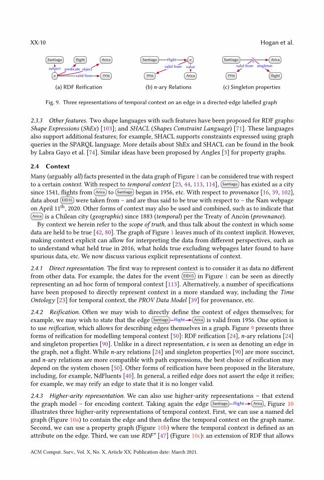
Fig. 9. Three representations of temporal context on an edge in a directed-edge labelled graph
2.3.3 Other features. Two shape languages with such features have been proposed for RDF graphs:
Shape Expressions (ShEx) [103]; and SHACL (Shapes Constraint Language) [71]. These languages
also support additional features; for example, SHACL supports constraints expressed using graph
queries in the SPARQL language. More details about ShEx and SHACL can be found in the book
by Labra Gayo et al. [74]. Similar ideas have been proposed by Angles [3] for property graphs.
2.4 ContextMany (arguably all) facts presented in the data graph of Figure 1 can be considered true with respect
to a certain context. With respect to temporal context [23, 44, 113, 114], Santiago has existed as a city
since 1541, flights from Arica to Santiago began in 1956, etc. With respect to provenance [16, 39, 102],
data about EID15 were taken from – and are thus said to be true with respect to – the Ñam webpage
on April 11th, 2020. Other forms of context may also be used and combined, such as to indicate that
Arica is a Chilean city (geographic) since 1883 (temporal) per the Treaty of Ancón (provenance).
By context we herein refer to the scope of truth, and thus talk about the context in which some
data are held to be true [42, 80]. The graph of Figure 1 leaves much of its context implicit. However,
making context explicit can allow for interpreting the data from different perspectives, such as
to understand what held true in 2016, what holds true excluding webpages later found to have
spurious data, etc. We now discuss various explicit representations of context.
2.4.1 Direct representation. The first way to represent context is to consider it as data no different
from other data. For example, the dates for the event EID15 in Figure 1 can be seen as directly
representing an ad hoc form of temporal context [113]. Alternatively, a number of specifications
have been proposed to directly represent context in a more standard way, including the Time
Ontology [23] for temporal context, the PROV Data Model [39] for provenance, etc.
2.4.2 Reification. Often we may wish to directly define the context of edges themselves; for
example, we may wish to state that the edge Santiago Aricaflight is valid from 1956. One option is
to use reification, which allows for describing edges themselves in a graph. Figure 9 presents three
forms of reification for modelling temporal context [50]: RDF reification [24], n-ary relations [24]
and singleton properties [90]. Unlike in a direct representation, e is seen as denoting an edge in
the graph, not a flight. While n-ary relations [24] and singleton properties [90] are more succinct,
and n-ary relations are more compatible with path expressions, the best choice of reification may
depend on the system chosen [50]. Other forms of reification have been proposed in the literature,
including, for example, NdFluents [40]. In general, a reified edge does not assert the edge it reifies;
for example, we may reify an edge to state that it is no longer valid.
2.4.3 Higher-arity representation. We can also use higher-arity representations – that extend
the graph model – for encoding context. Taking again the edge Santiago Aricaflight , Figure 10
illustrates three higher-arity representations of temporal context. First, we can use a named del
graph (Figure 10a) to contain the edge and then define the temporal context on the graph name.
Second, we can use a property graph (Figure 10b) where the temporal context is defined as an
attribute on the edge. Third, we can use RDF* [47] (Figure 10c): an extension of RDF that allows
ACM Comput. Surv., Vol. X, No. X, Article XX. Publication date: March 2021.

Knowledge Graphs XX:11
Santiago Aricaflight
e 1956valid from
(a) Named graph
Santiago Arica
valid from = 1956
e : flight
(b) Property graph
Santiago Aricaflight 1956valid from
(c) RDF*
Fig. 10. Three higher-arity representations of temporal context on an edge
SantiagoArica flight{[1, 125], [200, 365]}
EID17
city{[276, 279]}
EID16
city{[123, 130]}
Punta Arenasflight{[1, 120], [220, 365]}
EID18
city{[150, 152]}
G: Santiago ?cityflight ?eventcityQ :
Q (G) :?city context
Arica {[123, 125], [276, 279]}
Fig. 11. Example query on a temporally annotated graph
edges to be defined as nodes. The most flexible of the three is the named graph representation, where
we can assign context to multiple edges at once by placing them in one named graph, for example,
adding more edges valid from 1956 to the named graph of Figure 10a. The least flexible option is
RDF*, which, without an edge id, cannot capture different groups of contextual values on an edge;
for example, we can add four values to the edge Chile M. Bacheletpresident stating that it was valid
from 2006 until 2010 and valid from 2014 until 2018, but we cannot pair the values [50, 114].
2.4.4 Annotations. While the previous alternatives are concerned with representing context, an-
notations allow for defining contexts, which enables automated context-aware processing of data.
Some annotations model a particular contextual domain; for example, Temporal RDF [44] allows for
annotating edges with time intervals, such as Chile M. Bacheletpresident
[2006, 2010] , while Fuzzy RDF [124]
allows for annotating edges with a degree of truth such as Santiago Semi-Aridclimate0.8
, indicating
that it is more-or-less true – with a degree of 0.8 – that Santiago has a semi-arid climate.
Other frameworks are domain-independent. Annotated RDF [30, 133, 155] allows for representing
various forms of context modelled as semi-rings: algebraic structures consisting of domain values
(e.g., temporal intervals, fuzzy values, etc.) and two main operators to combine domain values:meet
and join (different from the relational algebra operator). Figure 11 gives an example where G is
annotated with integers (1–365) denoting days of the year. We use an interval notation such that
{[150, 152]} indicates the set {150, 151, 152}. Query Q asks for flights from Santiago to cities with
events and returns the temporal validity of each answer. To derive these answers, we first apply
the meet operator – defined here as set intersection – to compute the annotation for which a flightand city edge hold; for example, applying meet on {[150,152]} and {[1,120],[220,365]} for Punta Arenas
gives the empty time interval {}, and thus it may be omitted from the results (depending on the
semantics chosen). However, for Arica , we find two non-empty intersections: {[123,125]} for EID16
and {[276,279]} for EID17 . Since we are interested in the city, rather than the event, we combine these
two annotations for Arica using the join operator, returning the annotation in which either result
holds true. In our scenario, we define join as the union of sets, giving {[123,125],[276,279]}.
2.4.5 Other contextual frameworks. Other frameworks for modelling and reasoning about context
in graphs include that of contextual knowledge repositories [57], which assign (sub-)graphs to
contexts with one or more partially-ordered dimensions (e.g., 2020-03-22 ≼ 2020-03 ≼ 2020 ) allowing to
select sub-graphs at different levels of contextual granularity. A similar framework, proposed by
Schuetz et al. [119], is based on OLAP-like operations over contextual dimensions.
ACM Comput. Surv., Vol. X, No. X, Article XX. Publication date: March 2021.

XX:12 Hogan et al.
Q : ?festivalFestival
type
Santiagolocation
?name name
Fig. 12. Graph pattern querying for names of festivals in Santiago
3 DEDUCTIVE KNOWLEDGEAs humans, we can deduce more from the data graph of Figure 1 than what the edges explicitly
indicate. We may deduce, for example, that the Ñam festival ( EID15 ) will be located in Santiago, that
the cities connected by flights must have some airport nearby, etc. Given the data as premises, and
some general rules about the world that we may know a priori, we can use a deductive process to
derive new data, allowing us to know more than what is explicitly given to us by the data.
Machines do not have inherent deductive faculties, but rather need entailment regimes to formalise
the logical consequence of a given set of premises. Once instructed in this manner, machines can
(often) apply deductions with a precision, efficiency, and scale beyond human performance. These
deductions may serve a range of applications, such as improving query answering, (deductive)
classification, finding inconsistencies, etc. As an example, take the query in Figure 12 asking for the
festivals located in Santiago. The query returns no results for the graph in Figure 1: there is no node
with type Festival , and nothing has the location Santiago . However, an answer ( Ñam ) could be entailed
if we stated that x being a Food Festival entails that x is a Festival, or that x having venue y in city
z entails that x has location z. Entailment regimes automate such deductions.
In this section, we discuss ways in which potentially complex entailments can be expressed and
automated. Though we could leverage a number of logical frameworks for these purposes – such as
First-Order Logic, Datalog, Prolog, Answer Set Programming, etc. – we focus on ontologies, which
constitute a formal representation of knowledge that, importantly for us, can be represented as a
graph; in other words, ontologies can be seen as knowledge graphs with well-defined meaning [32].
3.1 OntologiesTo enable entailment, we must be precise about what the terms we use mean. For example, we have
referred to the nodes EID15 and EID16 in Figure 1 as “events”. But what if, for example, we wish to
define two pairs of start and end dates for EID16 corresponding to the different venues? Should we
rather consider what takes place in each venue as a different event? What if an event has various
start and end dates in a single venue: would these be considered one (recurring) event, or many
events? These questions are facets of a more general question: what do we mean by an “event”? The
term “event” may be interpreted in many ways, where the answers are a matter of convention.
In computing, an ontology is then a concrete, formal representation – a convention – on what
terms mean within the scope in which they are used (e.g., a given domain). Like all conventions,
the usefulness of an ontology depends on how broadly and consistently it is adopted, and how
detailed it is. Knowledge graphs that use a shared ontology will be more interoperable. Given that
ontologies are formal representations, they can further be used to automate entailment.
Amongst the most popular ontology languages used in practice are the Web Ontology Language
(OWL) [52], recommended by the W3C and compatible with RDF graphs; and the Open Biomedical
Ontologies Format (OBOF ) [88], used mostly in the biomedical domain. Since OWL is the more
widely adopted, we focus on its features, though many similar features are found in both [88].
Before introducing such features, however, we must discuss how graphs are to be interpreted.
3.1.1 Interpretations. We as humans may interpret the node Santiago in the data graph of Figure 1
as referring to the real-world city that is the capital of Chile. We may further interpret an edge
ACM Comput. Surv., Vol. X, No. X, Article XX. Publication date: March 2021.
Knowledge Graphs XX:13
Arica Santiagoflight as stating that there are flights from the city of Arica to this city. We thus
interpret the data graph as another graph – what we here call the domain graph – composed of
real-world entities connected by real-world relations. The process of interpretation, here, involves
mapping the nodes and edges in the data graph to nodes and edges of the domain graph.
We can thus abstractly define an interpretation [7] of a data graph as the combination of a domain
graph and a mapping from the terms (nodes and edge-labels) of the data graph to those of the
domain graph. The domain graph follows the same model as the data graph. We refer to the nodes
of the domain graph as entities, and the edges of the domain graph as relations. Given a node Santiago
in the data graph, we denote the entity it refers to in the domain graph (per a given interpretation)
by Santiago . Likewise, for an edge Arica Santiagoflight , we will denote the relation it refers to by
Arica Santiagoflight . In this abstract notion of an interpretation, we do not require that Santiago or
Arica be the real-world cities: an interpretation can have any domain graph and mapping.
3.1.2 Assumptions. Why is this abstract notion of interpretation useful? The distinction between
nodes/edges and entities/relations becomes clear when we define the meaning of ontology features
and entailment. To illustrate, if we ask whether there is an edge labelled flight between Arica and
Viña del Mar for the data graph in Figure 1, the answer is no. However, if we ask if the entities Arica
and Viña del Mar are connected by the relation flight, then the answer depends on what assumptions
we make when interpreting the graph. Under the Closed World Assumption (CWA) – which asserts
that what is not known is assumed false – without further knowledge the answer is no. Conversely,
under the Open World Assumption (OWA), it is possible for the relation to exist without being
described by the graph [7]. Under the Unique Name Assumption (UNA), which states that no two
nodes can map to the same entity, we can say that the data graph describes at least two flights
to Santiago (since Viña del Mar and Arica must be different entities). Conversely, under the No Unique
Name Assumption (NUNA), we can only say that there is at least one such flight since Viña del Mar
and Arica may be the same entity with two “names” (i.e., two nodes referring to the same entity).
These assumptions definewhich interpretations are valid, andwhich interpretations satisfy which
data graphs. The UNA forbids interpretations that map two nodes to the same entity, while the
NUNA does not. Under CWA, an interpretation that contains an edge x yp in its domain graph
can only satisfy a data graph from which we can entail x yp . Under OWA, an interpretation
containing the edge x yp can satisfy a data graph not entailing x yp so long it does not
contradict that edge. Ontologies typically adopt the NUNA and OWA, i.e., the most general case,
which considers that data may be incomplete, and two nodes may refer to the same entity.
3.1.3 Semantic conditions. Beyond our base assumptions, we can associate certain patterns in the
data graph with semantic conditions that define which interpretations satisfy it [7]; for example, we
can add a semantic condition on a special edge label subp. of (subproperty of) to enforce that if our
data graph contains the edge venue locationsubp. of , then any edge x yvenue in the domain graph
of the interpretation must also have a corresponding edge x ylocation in order to satisfy the data
graph. These semantic conditions then form the features of an ontology language.
3.1.4 Individuals. In Table 2, we list the main features supported by ontologies for describing
individuals [52] (aka., entities). First, we can assert (binary) relations between individuals using
edges such as Santa Lucía Santiagocity . In the condition column, whenwewrite x zy , for example,
we refer to the condition that the given relation holds in the interpretation; if so, the interpretation
satisfies the assertion. We may further assert that two terms refer to the same entity, where, e.g.,
Región V Región de Valparaísosame as states that both refer to the same region; or that two terms refer
to different entities, where, e.g., Valparaíso Región de Valparaísodiff. from distinguishes the city from the
region of the same name. We may also state that a relation does not hold using negation.
ACM Comput. Surv., Vol. X, No. X, Article XX. Publication date: March 2021.

XX:14 Hogan et al.
Table 2. Ontology features for individuals
Feature Axiom Condition Example
Assertion x zy x zy Chile Santiagocapital
Negation nx
sub
ypre
z
obj
Neg
type
not x zy nChile
sub
capitalpre
Arica
obj
Neg
type
Same As x1 x2same as x1 = x2 Región V Región de Valparaísosame as
Different From x1 x2diff. from x1 , x2 Valparaíso Región de Valparaísodiff. from
3.1.5 Properties. Properties denote terms that can be used as edge-labels [52]. We may use a
variety of features for defining the semantics of properties, as listed in Table 3. First we may define
subproperties as exemplified before. We may also associate classes with properties by defining
their domain and range. We may further state that a pair of properties are equivalent, inverses, or
disjoint, or define a particular property to denote a transitive, symmetric, asymmetric, reflexive, or
irreflexive relation. We can also define the multiplicity of the relation denoted by properties, based
on being functional (many-to-one) or inverse-functional (one-to-many). We may further define a
key for a class, denoting the set of properties whose values uniquely identify the entities of that
class. Without adopting a Unique Name Assumption (UNA), from these latter three features we
may conclude that two or more terms refer to the same entity. Finally, we can relate a property to
a chain (a path expression only allowing concatenation of properties) such that pairs of entities
related by the chain are also related by the given property. For the latter two features in Table 3 we
use the vertical notation... to represent lists (for example, OWL uses RDF lists [24]).
3.1.6 Classes. Often we can group nodes in a graph into classes – such as Event, City, etc. – with
a type property. Table 4 then lists a range of features for defining the semantics of classes. First,
subclass can be used to define class hierarchies.We can further define pairs of classes to be equivalent,
or disjoint. We may also define novel classes based on set operators: as being the complement of
another class, the union or intersection of a list of other classes, or as an enumeration of all of its
instances. One can also define classes based on restrictions on the values its instances take for a
property p, such as defining the class that has some value or all values from a given class on p;4
have a specific individual (has value) or themselves (has self ) as a value on p; have at least, at most
or exactly some number of values on p (cardinality); and have at least, at most or exactly some
number of values on p from a given class (qualified cardinality). For the latter two cases, in Table 4,
we use the notation “#{ a | ϕ}” to count distinct entities satisfying ϕ in the interpretation. Features
can be combined to create complex classes, where combining the examples for Intersection and
Has Self in Table 4 gives the definition: self-driving taxis are taxis having themselves as a driver.
3.1.7 Other features. Ontology languages may support further features, including datatype vs.
object properties, which distinguish properties that take datatype values from those that do not;
and datatype facets, which allow for defining new datatypes by applying restrictions to existing
datatypes, such as to define that places in Chile must have a float between -66.0 and -110.0 as their
value for the (datatype) property latitude. For more details we refer to the OWL 2 standard [52].
4While DomesticAirport NationalFlightallflight prop might be a tempting definition, its condition would be vacuously
satisfied by individuals that cannot have any flight (e.g., an instance of Bus Station where Bus Station 0=flight prop ).
ACM Comput. Surv., Vol. X, No. X, Article XX. Publication date: March 2021.

Knowledge Graphs XX:15
Table 3. Ontology features for property axioms
Feature Axiom Condition (for all x∗, y∗, z∗) Example
Subproperty p qsubp. of x yp implies x yq venue locationsubp. of
Domain p cdomain x yp implies x ctype venue Eventdomain
Range p crange x yp implies y ctype venue Venuerange
Eqivalence p qequiv. p. x yp iff x yq start beginsequiv. p.
Inverse p qinv. of x yp iff y xq venue hostsinv. of
Disjoint p qdisj. p. not x ypq
venue hostsdisj. p.
Transitive p Transitivetype x yp zp implies x zp part of Transitivetype
Symmetric p Symmetrictype x yp iff y xp nearby Symmetrictype
Asymmetric p Asymmetrictype not x ypp
capital Asymmetrictype
Reflexive p Reflexivetype x p part of Reflexivetype
Irreflexive p Irreflexivetype not x p flight Irreflexivetype
Functional p Functionaltype y1 xp y2p implies y1 = y2 population Functionaltype
Inv. Functional p Inv. Functionaltype x1 yp x2p implies x1 = x2 capital Inv. Functionaltype
Key cp1...pn
key x1
c
type
x2
typey1p1 p1
...... ...
yn
pn pn
implies x1 = x2 City latlongkey
Chain pq1...qn
chainx y1q1 yn−1... zqn. implies x zp
location locationpart ofchain
3.2 Semantics and EntailmentThe conditions listed in the previous tables give rise to entailments; for example, the definition
nearby Symmetrictype and edge Santiago Santiago Airportnearby entail Santiago Airport Santiagonearby per
the Symmetric condition of Table 3. We now describe how these conditions lead to entailments.
3.2.1 Model-theoretic semantics. Each axiom described by the previous tables, when added to a
graph, enforces some condition(s) on the interpretations that satisfy the graph. The interpretations
that satisfy a graph are calledmodels of the graph [7]. If we considered only the base condition of the
Assertion feature in Table 2, for example, then the models of a graph would be any interpretation
such that for every edge x zy in the graph, there exists a relation x zy in the model. Given
that there may be other relations in the model (under the OWA), the number of models of any such
graph is infinite. Furthermore, given that we can map multiple nodes in the graph to one entity
in the model (under the NUNA), any interpretation with (for example) the relation a aa is
a model of any graph so long as for every edge x zy in the graph, it holds that x = y = z
= a in the interpretation (in other words, the interpretation maps everything to a ). As we add
axioms with their associated conditions to the graph, we restrict models for the graph; for example,
considering a graph with two edges – x zy and y Irreflexivetype – the interpretation with
a aa , x = y = ... = a is no longer a model as it breaks the condition for the irreflexive axiom.
ACM Comput. Surv., Vol. X, No. X, Article XX. Publication date: March 2021.

XX:16 Hogan et al.
Table 4. Ontology features for class axioms and definitions
Feature Axiom Condition (for all x∗, y∗, z∗) Example
Subclass c dsubc. of x ctype implies x dtype City Placesubc. of
Eqivalence c dequiv. c. x ctype iff x dtype Human Personequiv. c.
Disjoint c ddisj. c. not c xtype dtype City Regiondisj. c.
Complement c dcomp. x ctype iff not x dtype Dead Alivecomp.
Union cd1...dn
union x ctype iff
x d1type or
x ...type or
x dntype
Flight DomesticFlightInternationalFlightunion
Intersection cd1...dn
inter. x ctype iff x ...type
d1
type
dn
typeSelfDrivingTaxi Taxi
SelfDrivinginter.
Enumeration cx1...xn
one of x ctype iff x ∈ { x1 , . . . , xn } EUState
Austria...
Swedenone of
Some Values cd
some
pprop x ctype iff
there exists a such that
x ap dtypeEUCitizen
EUStatesome
nationalityprop
All Values cd
all
pprop x ctype iff
for all a with x ap
it holds that a dtypeWeightless
Weightlessall
has partprop
Has Value cyvalue
pprop x ctype iff x yp ChileanCitizen
Chilevalue
nationalityprop
Has Self ctrue
self
pprop x ctype iff x xp SelfDriving
trueself
driverprop
Cardinality
⋆ ∈ {=, ≤, ≥}c
n⋆
pprop x ctype iff
. #{ a | x ap } ⋆ nPolyglot
2≥
fluentprop
Qualified
Cardinality
⋆ ∈ {=, ≤, ≥}
c dclass
n⋆
pprop x ctype iff
. #{ a | x ap dtype } ⋆ nBinaryStarSystem Starclass
2
=
bodyprop
3.2.2 Entailment. We say that one graph entails another if and only if any model of the former
graph is also a model of the latter graph [7]. Intuitively this means that the latter graph says
nothing new over the former graph and thus holds as a logical consequence of the former graph. For
example, consider the graph Santiago Citytype Placesubc. of and the graph Santiago Placetype . All
models of the latter must have that Santiago Placetype , but so must all models of the former, which
must have Santiago Citytype Placesubc. of and further must satisfy the condition for Subclass,
which requires that Santiago Placetype also hold. Hence we conclude that any model of the former
graph must be a model of the latter graph, and thus the former graph entails the latter graph.
3.3 ReasoningGiven two graphs, deciding if the first entails the second – per all of the features in Tables 2–4
– is undecidable: no (finite) algorithm for such entailment can exist that halts on all inputs with
the correct true/false answer [53]. However, we can provide practical reasoning algorithms for
ontologies that (1) halt on any input ontology but may miss entailments, returning false instead
ACM Comput. Surv., Vol. X, No. X, Article XX. Publication date: March 2021.

Knowledge Graphs XX:17
O : locationcityvenue
chain FestivalFood Festival subc. of Drinks Festivalsubc. of
O(Q) :( ?festival Festivaltype ∪ ?festival Food Festivaltype ∪ ?festival Drinks Festivaltype )
Z ( ?festival Santiagolocation ∪ ?festival ?xvenue Santiagocity ) Z ?festival ?namename
Fig. 13. Query rewriting example for the query Q of Figure 12
of true, (2) always halt with the correct answer but only accept input ontologies with restricted
features, or (3) only return correct answers for any input ontology but may never halt on certain
inputs. Though option (3) has been explored using, e.g., theorem provers for First Order Logic [118],
options (1) and (2) are more commonly pursued using rules and/or Description Logics. Option (1)
often allows for more efficient and scalable reasoning algorithms and is useful where data are
incomplete and having some entailments is valuable. Option (2) may be a better choice in domains
– such as medical ontologies – where missing entailments may have undesirable outcomes.
3.3.1 Rules. A straightforward way to implement reasoning is through inference rules (or simply
rules), composed of a body (if) and a head (then). Both the body and head are given as graph
patterns. A rule indicates that if we can replace the variables of the body with terms from the data
graph and form a subgraph of a given data graph, then using the same replacement of variables
in the head will yield a valid entailment. The head must typically use a subset of the variables
appearing in the body to ensure that the conclusion leaves no variables unreplaced. Rules of this
form correspond to (positive) Datalog in databases, Horn clauses in logic programming, etc.
Rules can be used to capture entailments under ontological conditions. Here we provide an
example of two rules for capturing some of the entailments valid for Subclass:
?x ?ctype ?dsubc. of ⇒ ?x ?dtype
?c ?dsubc. of ?esubc. of ⇒ ?c ?esubc. of
A comprehensive set of rules for OWL have been standardised as OWL 2 RL/RDF [86]. These
rules are, however, incomplete as such rules cannot fully capture negation (e.g., Complement),
existentials (e.g., Some Values), universals (e.g., All Values), or counting (e.g., Cardinality and
Qualified Cardinality). Other rule languages can, however, support additional such features,
including existentials (see, e.g., Datalog±[12]), disjunction (see, e.g., Disjunctive Datalog [112]), etc.
Rules can be used for reasoning in a number of ways.Materialisation applies rules recursively to a
graph, adding entailments back to the graph until nothing new can be added. The materialised graph
can then be treated as any other graph; however the materialised graph may become unfeasibly
large to manage. Another strategy is to use rules for query rewriting, which extends an input query
in order to find entailed solutions. Figure 13 provides an example ontology whose rules are used to
rewrite the query of Figure 12; if evaluated over the graph of Figure 1, Ñam will be returned as a
solution. While not all ontological features can be supported in this manner, query rewriting is
sufficient to support complete reasoning over lightweight ontology languages [86].
While rules can be used to (partially) capture ontological entailments, they can also be defined
independently of an ontology, capturing entailments for a given domain. In fact, some rules – such
as the following – cannot be emulated with the ontology features previously seen, as they do not
support ways to infer binary relations from cyclical graph patterns (for computability reasons):
?x ?yflight ?z
countrycountry ⇒ ?x ?ydomestic flight
Various languages allow for expressing rules over graphs (possibly alongside ontological definitions)
including: Rule Interchange Format (RIF) [69], Semantic Web Rule Language [58], etc.
ACM Comput. Surv., Vol. X, No. X, Article XX. Publication date: March 2021.

XX:18 Hogan et al.
3.3.2 Description Logics. Description Logics (DLs) hold an important place in the logical formali-
sation of knowledge graphs: they were initially introduced as a way to formalise the meaning of
frames [84] and semantic networks [106] (which can be seen as predecessors of knowledge graphs)
and also heavily influenced OWL. DLs are a family of logics rather than a particular logic. Initially,
DLs were restricted fragments of First Order Logic (FOL) that permit decidable reasoning tasks,
such as entailment checking [7]. DLs would later be extended with useful features for modelling
graph data that go beyond FOL, such as transitive closure, datatypes, etc. Different DLs strike
different balances between expressive power and the computational complexity of reasoning.
DLs are based on three types of elements: individuals, such as Santiago; classes (aka concepts) suchas City; and properties (aka roles) such as flight. DLs then allow for making claims, known as axioms,
about these elements. Assertional axioms can be either unary class relations on individuals, such as
City(Santiago), or binary property relations on individuals, such as flight(Santiago,Arica). Such axioms
form the Assertional Box (A-Box). DLs further introduce logical symbols to allow for defining class
axioms (forming the Terminology Box, or T-Box for short), and property axioms (forming the Role
Box, or R-Box); for example, the class axiom City ⊑ Place states that the former class is a subclass
of the latter one, while the property axiom flight ⊑ connectsTo states that the former property is
a subproperty of the latter one. DLs also allow for defining classes based on existing terms; for
example, we can define a class ∃nearby.Airport as the class of individuals that have some airport(s)
nearby. Noting that the symbol ⊤ is used in DLs to denote the class of all individuals, we can then
add a class axiom ∃flight.⊤ ⊑ ∃nearby.Airport to state that individuals with an outgoing flight must
have some airport nearby. Noting that the symbol ⊔ can be used in DL to define that a class is the
union of other classes, we can further define that Airport ⊑ DomesticAirport ⊔ InternationalAirport,i.e., that an airport is either a domestic airport or an international airport (or both).
The similarities between DLs and OWL are not coincidental: the OWL standard was heavily
influenced by DLs, where the OWL 2 DL language is a restricted fragment of OWL with decidable
entailment. To exemplify one such restriction, with DomesticAirport ⊑ =1 destination ◦ country.⊤we can define in DL syntax that domestic airports have flights destined to precisely one country
(where p ◦ q denotes a chain of properties). However, counting chains is often disallowed in DLs to
ensure decidability. For further reading, we refer to the textbook by Baader et al. [7].
Expressive DLs support complex entailments involving existentials, universals, counting, etc.
A common strategy for deciding such entailments is to reduce entailment to satisfiability, which
decides if an ontology is consistent or not.5Thereafter methods such as tableau can be used to
check satisfiability, cautiously constructing models by completing them along similar lines to the
materialisation strategy previously described, but additionally branching models in the case of
disjunction, introducing new elements to represent existentials, etc. If any model is successfully
“completed”, the process concludes that the original definitions are satisfiable (see, e.g., [87]). Due to
their prohibitive computational complexity [86], such reasoning strategies are not typically applied
to large-scale data, but may be useful when modelling complex domains.
4 INDUCTIVE KNOWLEDGEInductive reasoning generalises patterns from input observations, which are used to generate
novel but potentially imprecise predictions. For example, from a graph with geographical and
flight information, we may observe that almost all capital cities of countries have international
airports serving them, and hence predict that since Santiago is a capital city, it likely has an
international airport serving it; however, some capitals (e.g., Vaduz) do not have international
airports. Predictions may thus have a level of confidence; for example, if we see that 187 of 195
5G entails G′if and only if G ∪ not(G′) is not satisfiable.
ACM Comput. Surv., Vol. X, No. X, Article XX. Publication date: March 2021.

Knowledge Graphs XX:19
Inductive Knowledge
Symbolic
Self-supervised
Axiom MiningRule Mining
Numeric
Supervised
GNNs
Self-supervised
Embeddings
Unsupervised
Graph Analytics
Fig. 14. Conceptual overview of inductive techniques for knowledge graphs
Calama
San Pedro
bus
Piedras Rojas
Moon Valley
busbus
Los Flamencos
bus bus
Santiago
flight
Arica
flightbus
Iquique
flight
flight
Easter Island
flight
Puerto Monttflight
Punta Arenas
flightflight
bus
Puerto Varas
busbus
Torres del Painebus
Grey Glacier
busbus
Osorno Volcanobus
Fig. 15. Data graph representing transport routes in Chile
capitals have an international airport, we may assign a confidence of 0.959 for predictions made
with that pattern. We then refer to knowledge acquired inductively as inductive knowledge, which
includes both the models that encode patterns, and the predictions made by those models.
Inductive knowledge can be acquired from graphs using supervised or unsupervised methods.
Supervised methods learn a function (aka model) to map a set of example inputs to their labelled
outputs; the model can then be applied to unlabelled inputs. To avoid costly labelling, some
supervised methods can generate the input–output pairs automatically from the (unlabelled) input,
which are then fed into a supervised process to learn a model; herein we refer to this approach as
self-supervision. Alternatively, unsupervised processes do not require labelled input–output pairs,
but rather apply a predefined function (typically statistical in nature) to map inputs to outputs.
In Figure 14 we provide an overview of the inductive techniques typically applied to knowledge
graphs. In the case of unsupervised methods, there is a rich body of work on graph analytics,
wherein well-known algorithms are used to detect communities or clusters, find central nodes and
edges, etc., in a graph. Alternatively, knowledge graph embeddings use self-supervision to learn a
low-dimensional numerical model of elements of a knowledge graph. The structure of graphs can
also be directly leveraged for supervised learning through graph neural networks. Finally, symbolic
learning can learn symbolic models – i.e., logical formulae in the form of rules or axioms – from a
graph in a self-supervised manner. We now discuss each of the aforementioned techniques in turn.
4.1 Graph AnalyticsGraph analytics is the application of analytical algorithms to (often large) graphs. Such algorithms
often analyse the topology of the graph, i.e., how nodes and groups thereof are connected. In this
section, we provide a brief overview of some popular graph algorithms applicable to knowledge
graphs, and then discuss graph processing frameworks onwhich such algorithms can be implemented.
4.1.1 Graph algorithms. A wide variety of graph algorithms can be applied for analytical purposes,
where we briefly introduce five categories of algorithms that are often used in practice [61].
First, centrality analysis aims to identify the most important (“central”) nodes or edges of a graph.
Specific node centrality measures include degree, betweenness, closeness, Eigenvector, PageRank,
HITS, Katz, among others. Betweenness centrality can also be applied to edges. A node centrality
ACM Comput. Surv., Vol. X, No. X, Article XX. Publication date: March 2021.

XX:20 Hogan et al.
Easter Island
AricaCalamaIquique
Puerto MonttPunta ArenasSantiago
flight
flight
Grey GlacierLos FlamencosMoon Valley
Osorno VolcanoPiedras RojasPuerto VarasSan Pedro
Torres del Paine
bus
bus
Fig. 16. Example quotient graph summarising the data graph in Figure 15
measure would allow, e.g., to predict the busiest transport hubs in Figure 15, while edge centrality
would allow us to find the edges on which many shortest routes depend for predicting traffic.
Second, community detection aims to identify sub-graphs that are more densely connected
internally than to the rest of the graph (aka. communities). Community detection algorithms include
minimum-cut algorithms, label propagation, Louvain modularity, etc. Community detection applied
to Figure 15 may, for example, detect a community to the left (referring to the north of Chile), to the
right (referring to the south of Chile), and perhaps also the centre (referring to cities with airports).
Third, connectivity analysis aims to estimate how well-connected and resilient the graph is.
Specific techniques include measuring graph density or k-connectivity, detecting strongly connected
components and weakly connected components, computing spanning trees or minimum cuts, etc. In
the context of Figure 15, such analysis may tell us that routes to Osorno Volcano and Piedras Rojas are the
most “brittle”, becoming disconnected from the main hubs if one of two bus routes fail.Fourth, node similarity aims to find nodes that are similar to other nodes by virtue of how they are
connected within their neighbourhood. Node similarity metrics may be computed using structural
equivalence, random walks, diffusion kernels, etc. These methods provide an understanding of what
connects nodes, and in what ways they are similar. In Figure 15, such analysis may tell us that
Calama and Arica are similar nodes as both have return flights to Santiago and return buses to San Pedro .
Fifth, graph summarisation aims to extract high-level structures from a graph, often based on
quotient graphs, where nodes in the input graph are merged while preserving the edges between the
input nodes [21, 56]. Such methods help to provide an overview for a large-scale graph. Figure 16
provides an example of a quotient graph that summarises the graph of Figure 15, such that if there
is an edge s op in the input graph, there is an edge S Op in the quotient graph with s ∈ Sand o ∈ O . In this case, quotient nodes are defined in terms of outgoing edge-labels, where we may
detect that they represent islands, cities, and towns/attractions, respectively, from left to right.
Many such techniques have been proposed and studied for simple graphs or directed graphs
without edge labels. An open research challenge in the context of knowledge graphs is to adapt such
algorithms for graph models such as del graphs, heterogeneous graphs and property graphs [15].
4.1.2 Graph processing frameworks. Various graph parallel frameworks have been proposed for
large-scale graph processing, including Apache Spark (GraphX) [26, 147], GraphLab [77], Pregel [79],
Signal–Collect [125], Shark [148], etc. Computation in these frameworks is iterative, where in each
iteration, each node reads messages received through inward edges (and possibly its own previous
state), performs a computation, and then sends messages through outward edges using the result.
To illustrate, assume we wish to compute the places that are most (or least) easily reached in the
graph of Figure 15. A good way to measure this is using centrality, where we choose PageRank [95],
which computes the probability of a tourist that randomly follows the routes shown in the graph
being at a particular place after a given number of “hops”. We can implement PageRank on large
graphs using a graph parallel framework. In Figure 17, we provide an example of an iteration of
PageRank for a sub-graph of Figure 15. The nodes are initialised with a score of1
|V |= 1
6 : a tourist
ACM Comput. Surv., Vol. X, No. X, Article XX. Publication date: March 2021.

Knowledge Graphs XX:21
Piedras Rojas
Los Flamencos
d6·1
San Pedro
d6·1
d6·4
Calama
d6·4
d6·1
Arica
d6·4
d6·1
Moon Valley
d6·4
d6·1
Msg (iter = 1)
1
6
1
6
1
6
1
6
1
6
1
6
Piedras Rojas
Los Flamencos
d6·1
San Pedro
d6·1
d6·4
Calama
d6·4
d6·1
Arica
d6·4
d6·1
Moon Valley
d6·4
d6·1
Agg (iter = 1)
d6·4+ 1−d
6
d6·1+ 1−d
6
d6·4+ d
6·1+ 1−d
6
d6·1+ d
6·1+ d
6·1+ 1−d
6
d6·4+ 1−d
6
d6·4+ 1−d
6
Fig. 17. Example of a graph-parallel iteration of PageRank for a sample sub-graph of Figure 15
is assumed to have an equal chance of starting at any point. In the message phase (Msg), each node
v passes a score ofdRi (v )
|E(v )| on each of its outgoing edges, where we denote by d a “damping factor”
(typically d = 0.85) used to ensure convergence, by Ri (v) the score of node v in iteration i (theprobability of the tourist being at node v after i hops), and by |E(v)| the number of outgoing edges
of v . The aggregation phase (Agg) for v then sums all incoming messages along with its share of
the damping factor (1−d|V |
) to compute Ri+1(v). We then proceed to the message phase of the next
iteration, continuing until some termination criterion is reached and results are output.
While the given example is for PageRank, this abstraction is general enough to support a wide
variety of (though not all [149]) graph algorithms. An algorithm in this framework consists of the
functions to compute message values (Msg), and to accumulate messages (Agg). The framework
will then take care of distribution, message passing, fault tolerance, etc.
4.2 Knowledge Graph EmbeddingsMachine learning can be used for directly refining a knowledge graph [99]; or for downstream tasks
using the knowledge graph, such as recommendation [154], information extraction [134], question
answering [59], query relaxation [138], query approximation [45], etc. However, machine learning
techniques typically assume dense numeric representations (e.g., vectors), distinct from how graphs
are usually expressed. So how can graphs be encoded numerically for machine learning purposes?
A first attempt to represent a graph using vectors would be to use a one-hot encoding, generating
a vector of length |L| · |V | for each node – with |V | the number of nodes in the input graph and |L|the number of edge labels – placing a one at the corresponding index to indicate the existence of
the respective edge in the graph, or zero otherwise. Such a representation will, however, typically
result in large and sparse vectors, which will be detrimental for most machine learning models.
The main goal of knowledge graph embedding techniques is to create a dense representation of
the graph (i.e., embed the graph) in a continuous, low-dimensional vector space that can then be
used for machine learning tasks. The dimensionality d of the embedding is fixed and typically low
(often, e.g., 50 ≥ d ≥ 1000). Typically the graph embedding is composed of an entity embedding
for each node: a vector with d dimensions that we denote by e; and a relation embedding for each
edge label: (typically) a vector with O(d) dimensions that we denote by r. The overall goal of thesevectors is to abstract and preserve latent structures in the graph. There are many ways in which
this notion of an embedding can be instantiated. Most commonly, given an edge s op , a specific
embedding approach defines a scoring function that accepts es (the entity embedding of node s ), rp(the relation embedding of edge label p) and eo (the entity embedding of node o ) and computes the
plausibility of the edge: how likely it is to be true. Given a data graph, the goal is then to compute
the embeddings of dimension d that maximise the plausibility of positive edges (typically edges in
the graph) and minimise the plausibility of negative examples (typically edges in the graph with a
ACM Comput. Surv., Vol. X, No. X, Article XX. Publication date: March 2021.

XX:22 Hogan et al.
Valparaíso Santiagowest of
Curico
north of
Licantén west of
north of
Toconao
north of
Antofagasta
north of
(a) Original graph
rwo.
rno.
(b) Relation embeddings
eA. eT.
eV. eS.
eL. eC.
rwo.
(c) Entity embeddings
Fig. 18. Toy example of two-dimensional relation and entity embeddings learnt by TransE
node or edge label changed such that they are no longer in the graph) according to the given scoring
function. The resulting embeddings can then be seen as models learnt through self-supervision
that encode (latent) features of the graph, mapping input edges to output plausibility scores.
Embeddings can then be used for a number of low-level tasks. The plausibility scoring function
can be used to assign confidence to edges (possibly extracted from an external source), or to
complete edges with missing nodes/edge labels (aka. link prediction). Additionally, embeddings will
typically assign similar vectors to similar terms, and can thus be used for similarity measures.
A wide range of knowledge graph embedding techniques have been proposed [139], where we
summarise the most prominent. First we discuss translational models where relations are seen as
translating subject entities to object entities. We then describe tensor decomposition models that
extract latent factors approximating the graph’s structure. Thereafter we discuss neural models based
on neural networks. Finally, we discuss language models based on word embedding techniques.
4.2.1 Translational models. Translational models interpret edge labels as transformations from
subject nodes (aka the source or head) to object nodes (aka the target or tail); for example, in the
edge San Pedro Moon Valleybus , the edge label bus is seen as transforming San Pedro to Moon Valley , and
likewise for other bus edges. A seminal approach is TransE [17]. Over all positive edges s op ,
TransE learns vectors es, rp, and eo aiming to make es + rp as close as possible to eo. Conversely,if the edge is negative, TransE attempts to learn a representation that keeps es + rp away from
eo. Figure 18 provides a toy example of two-dimensional (d = 2) entity and relation embeddings
computed by TransE. We keep the orientation of the vectors similar to the original graph for clarity.
For any edge s op in the original graph, adding the vectors es+ rp should approximate eo. In this
toy example, the vectors correspond precisely where, for instance, adding the vectors for Licantén
(eL.) and west of (rwo.) gives a vector corresponding to Curico (eC.). We can use these embeddings to
predict edges (among other tasks); for example, in order to predict which node in the graph is most
likely to be west of Antofagasta (A.), by computing eA. + rwo. we find that the resulting vector (dotted
in Figure 18c) is closest to eT., thus predicting Toconao (T.) to be the most plausible such node.
Aside from this toy example, TransE can be too simplistic; for example, in Figure 15, bus notonly transforms San Pedro to Moon Valley , but also to Arica , Calama , where TransE will try to give similar
vectors to all such target locations, which may not be feasible given other edges. To resolve such
issues, many variants of TransE have been investigated, typically using a distinct hyperplane
(e.g., TransH [143]) or vector space (e.g., TransR [76], TransD [63]) for each type of relation.
Recently, RotatE [129] proposes translational embeddings in complex space, which allows to
capture more characteristics of relations, such as direction, symmetry, inversion, antisymmetry,
and composition. Embeddings have also been proposed in non-Euclidean space, e.g., MuRP [9] uses
relation embeddings that transform entity embeddings in the hyperbolic space of the Poincaré ball
mode, whose curvature provides more “space” to separate entities with respect to the dimensionality.
ACM Comput. Surv., Vol. X, No. X, Article XX. Publication date: March 2021.

Knowledge Graphs XX:23
A.C.L.S.T.V.
A.C.L.S.T.V.
west ofnorth of
0 0 0 1 0 0
0 0 0 0 0 0
0 0 0 0 0 0
0 1 0 0 0 0
0 0 0 0 0 0
0 0 0 0 0 0
x1
z1y1
xd
zdyd
≈ ⊗ + . . .+ ⊗
G ≈ x1 ⊗ y1 ⊗ z1 + . . .+ xd ⊗ yd ⊗ zd
Fig. 19. Abstract illustration of a CP d-rank decomposition of a tensor representing the graph of Figure 18a
4.2.2 Tensor decomposition models. A second approach to derive graph embeddings is to apply
methods based on tensor decomposition. A tensor is a multidimensional numeric field that generalises
scalars (0-order tensors), vectors (1-order tensors) and matrices (2-order tensors) towards arbitrary
dimension/order. Tensor decomposition involves decomposing a tensor into more “elemental”
tensors (e.g., of lower order) from which the original tensor can be recomposed (or approximated)
by a fixed sequence of basic operations. These elemental tensors can be seen as capturing latent
factors in the original tensor. There are many approaches to tensor decomposition, where we will
now briefly introduce the main ideas behind rank decompositions [107].
Leaving aside graphs, consider an (a × b)-matrix (i.e., an order-2 tensor) C, where each element
(C)i j denotes the average temperature of the ith city of Chile in the jth month of the year. Since
Chile is a long, thin country – ranging from subpolar to desert climates – we may decompose Cinto two vectors representing latent factors – x (with a elements) giving lower values for cities with
lower latitude, and y (with b elements), giving lower values for months with lower temperatures
– such that computing the outer product6of the two vectors approximates C reasonably well:
x ⊗ y ≈ C. If there exist x and y such that x ⊗ y = C, we call C a rank-1 matrix. Otherwise, the
rank r of C is the minimum number of rank-1 matrices we need to sum to get precisely C, i.e.,x1 ⊗ y1 + . . . xr ⊗ yr = C. In the temperature example, x2 ⊗ y2 might correspond to a correction for
altitude, x3 ⊗ y3 for higher temperature variance further south, etc. A (low) rank decomposition
of a matrix then sets a limit d on the rank and computes the vectors (x1, y1, . . . , xd , yd ) such that
x1 ⊗ y1 + . . . + xd ⊗ yd gives the best d-rank approximation of C. Noting that to generate n-ordertensors we need to compute the outer product of n vectors, we can generalise this idea towards low
rank decomposition of tensors; this method is called Canonical Polyadic (CP) decomposition [51].
To compute knowledge graph embeddings with such techniques, a graph can be encoded as a one-
hot order-3 tensor G with |V | × |L| × |V | elements, where the element (G)i jk = 1 if the ith node links
to the k th node with the jth edge label (otherwise (G)i jk = 0). A CP decomposition [51] can compute
a sequence of vectors (x1, y1, z1, . . . , xd , yd , zd ) such that x1 ⊗ y1 ⊗ z1 + . . . + xd ⊗ yd ⊗ zd ≈ G,
as illustrated in Figure 19. Letting X,Y,Z denote the matrices formed by
[x1 · · · xd
],
[y1 · · · yd
],[
z1 · · · zd], respectively, with each vector forming a matrix column, we can extract the ith row of
Y as an embedding for the ith relation, and the jth rows of X and Z as two embeddings for the jth
entity. However, knowledge graph embeddings typically aim to assign one vector to each entity.
DistMult [151] is a seminal method for computing knowledge graph embeddings based on rank
decompositions, where each entity and relation is associated with a vector of dimension d , such
that for an edge s op , a plausibility scoring function
∑di=1(es)i (rp)i (eo)i is defined, where (es)i ,
(rp)i and (eo)i denote the ith elements of vectors es, rp, eo, respectively. The goal, then, is to learn
6The outer product of two (column) vectors x of length a and y of length b , denoted x ⊗ y, is defined as xyT, yielding an(a × b)-matrix M such that (M)i j = (x)i · (y)j . Analogously, the outer product of k vectors is a k-order tensor.
ACM Comput. Surv., Vol. X, No. X, Article XX. Publication date: March 2021.

XX:24 Hogan et al.
vectors for each node and edge label that maximise the plausibility of positive edges and minimise
the plausibility of negative edges. This approach equates to a CP decomposition of the graph tensor
G, but where entities have one vector that is used twice: x1 ⊗ y1 ⊗ x1 + . . . + xd ⊗ yd ⊗ xd ≈ G. A
weakness of this approach is that per the scoring function, the plausibility of s op will always
be equal to that of o sp ; in other words, DistMult does not consider edge direction.
Rather than use a vector as a relation embedding, RESCAL [92] uses a matrix, which allows
for combining values from es and eo across all dimensions, and thus can capture (e.g.) edge direc-
tion. However, RESCAL incurs a higher cost in terms of space and time than DistMult. Recently,
ComplEx [131] and HolE [91] both use vectors for relation and entity embeddings, but ComplEx
uses complex vectors, while HolE uses a circular correlation operator (on reals) [56] in order to
capture edge-direction. SimplE [67] proposes to compute a standard CP decomposition, averaging
terms across X, Y, Z to compute the final plausibility scores. TuckER [10] employs a different
type of decomposition – called a Tucker Decomposition [132], which computes a smaller “core”
tensor T and a sequence of three matrices A, B and C, such that G ≈ T ⊗ A ⊗ B ⊗ C – where
entity embeddings are taken from A and C, while relation embeddings are taken from B. Of theseapproaches, TuckER [10] currently provides state-of-the-art results on standard benchmarks.
4.2.3 Neural models. A number of approaches rather use neural networks in order to learn knowl-
edge graph embeddings with non-linear scoring functions for plausibility.
An early neural model was Semantic Matching Energy (SME) [41], which learns parameters
(aka weights: w, w′) for two functions – fw(es, rp) and дw′(eo, rp) – such that the dot product of
the result of both functions gives the plausibility score. Both linear and bilinear variants of fwand дw′ are proposed. Another early proposal was Neural Tensor Networks (NTN) [122], which
maintains a tensorW of weights and computes plausibility scores by combining the outer product
es ⊗W⊗ eo with rp and a standard neural layer over es and eo. The tensorW yields a high number
of parameters, limiting scalability [139]. Multi Layer Perceptron (MLP) [31] is a simpler model,
where es, rp and eo are concatenated and fed into a hidden layer to compute the plausibility score.
More recent models use convolutional kernels. ConvE [29] generates a matrix from es and rpby “wrapping” each vector over several rows and concatenating both matrices, over which (2D)
convolutional layers generate the embeddings. A disadvantage is that wrapping vectors imposes
an arbitrary two-dimensional structure on the embeddings. HypER [8] also uses convolutions, but
avoids such wrapping by applying a fully connected layer (called the “hypernetwork”) to rp in order
to generate relation-specific convolutional filters through which the embeddings are generated.
The presented approaches strike different balances in terms of expressivity and the number of
parameters than need to be trained. While more expressive models, such as NTN, may better fit
more complex plausibility functions over lower dimensional embeddings by using more hidden
parameters, simplermodels, such as that proposed byDong et al. [31], and convolutional networks [8,
29] that enable parameter sharing by applying the same (typically small) kernels over different
regions of a matrix, require handling fewer parameters overall and are more scalable.
4.2.4 Language models. Embedding techniques were first explored as a way to represent natural
language within machine learning frameworks, with word2vec [82] and GloVe [101] being two
seminal approaches. Both approaches compute embeddings for words based on large corpora of
text such that words used in similar contexts (e.g., “frog”, “toad”) have similar vectors.
Approaches for language embeddings can be applied for graphs. However, while graphs consist
of an unordered set of sequences of three terms (i.e., a set of edges), text in natural language consists
of arbitrary-length sequences of terms (i.e., sentences of words). Along these lines, RDF2Vec [108]
performs biased random walks on the graph and records the paths traversed as “sentences”, which
are then fed as input into the word2vec [82] model. An example of such a path extracted from
ACM Comput. Surv., Vol. X, No. X, Article XX. Publication date: March 2021.

Knowledge Graphs XX:25
Figure 15 might be, for example, San Pedro Calamabus Iquiqueflight Santiagoflight ; the paper experi-
ments with 500 paths of length 8 per entity. RDF2Vec also proposes a second mode where sequences
are generated for nodes from canonically-labelled sub-trees of which they are a root node, where the
paper experiments with sub-trees of depth 1 and 2. Conversely, KGloVe [22] is based on the GloVe
model. Much like how the original GloVe model [101] considers words that co-occur frequently in
windows of text to be more related, KGloVe uses personalised PageRank to determine the most
related nodes to a given node, whose results are then fed into the GloVe model.
4.2.5 Entailment-aware models. The embeddings thus far consider the data graph alone. But what
if an ontology or set of rules is provided? One may first consider using constraint rules to refine the
predictions made by embeddings. Wang et al. [140] use functional and inverse-functional definitions
as constraints (under UNA); for example, if we define that an event can have at most one value for
venue, the plausibility of edges that would assign multiple venues to an event is lowered.
More recent approaches rather propose joint embeddings that consider both the data graph and
rules. KALE [43] computes entity and relation embeddings using a translational model (specifically
TransE) that is adapted to further consider rules using t-norm fuzzy logics. With reference to
Figure 15, consider a simple rule ?x ?ybus ⇒ ?x ?yconnects to . We can use embeddings to assign
plausibility scores to new edges, such as e1: Piedras Rojas Moon Valleybus . We can further apply the
previous rule to generate a new edge e2: Piedras Rojas Moon Valleyconnects to from the predicted edge e1.But what plausibility should we assign to e2? Letting p1 and p2 be the current plausibility scores
of e1 and e2 (initialised using the standard embedding), then t-norm fuzzy logics suggests that
the plausibility be updated as p1p2 − p1 + 1. Embeddings are then trained to jointly assign larger
plausibility scores to positive examples of both edges and ground rules, i.e., rules with variables
replaced by constants from the graph, such as Arica San Pedrobus ⇒ Arica San Pedroconnects to .
Generating ground rules can be costly. An alternative approach, adopted by FSL [28], observes
that in the case of a simple rule, such as ?x ?ybus ⇒ ?x ?yconnects to , the relation embedding
bus should always return a lower plausibility than connects to. Thus, for all such rules, FSL pro-
poses to train relation embeddings while avoiding violations of such inequalities. While relatively
straightforward, FSL only supports simple rules, while KALE also supports more complex rules.
4.3 Graph Neural NetworksRather than compute numerical representations for graphs, an alternative is to define custom ma-
chine learning architectures for graphs. Most such architectures are based on neural networks [144]
given that a neural network is already a directed weighted graph, where nodes serve as artificial
neurons, and edges serve as weighted connections (axons). However, the topology of a traditional
(fully-connected feed-forward) neural network is quite homogeneous, having sequential layers of
fully-connected nodes. Conversely, the topology of a data graph is typically more heterogeneous.
A graph neural network (GNN) [116] is a neural network where nodes are connected to their
neighbours in the data graph. Unlike embeddings, GNNs support end-to-end supervised learning for
specific tasks: given a set of labelled examples, GNNs can be used to classify elements of the graph
or the graph itself. GNNs have been used to perform classification over graphs encoding compounds,
objects in images, documents, etc.; as well as to predict traffic, build recommender systems, verify
software, etc. [144]. Given labelled examples, GNNs can even replace graph algorithms; for example,
GNNs have been used to find central nodes in knowledge graphs in a supervisedmanner [97, 98, 116].
We now introduce two flavours of GNNs: recursive and convolutional.
4.3.1 Recursive graph neural networks. Recursive graph neural networks (RecGNNs) are the sem-
inal approach to graph neural networks [116, 123]. The approach is conceptually similar to the
ACM Comput. Surv., Vol. X, No. X, Article XX. Publication date: March 2021.
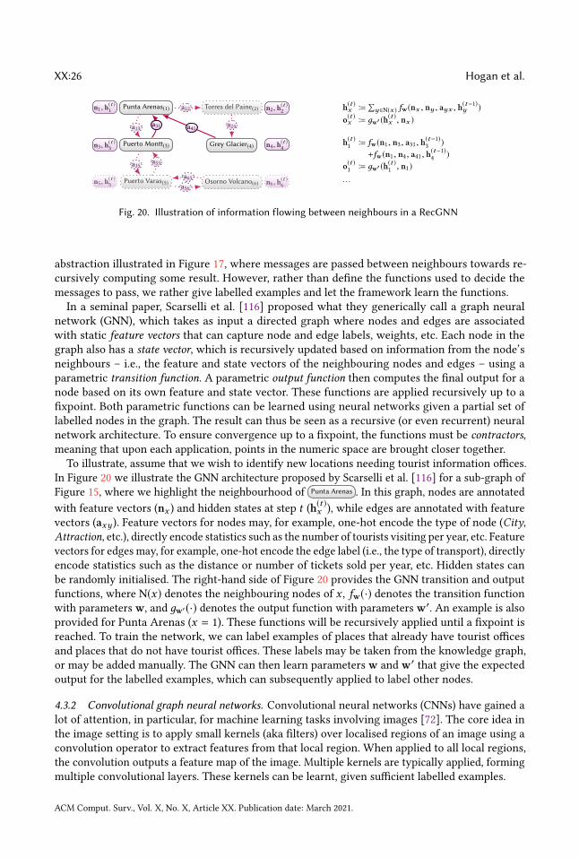
XX:26 Hogan et al.
Puerto Montt(3)n3, h(t )3
Punta Arenas(1)
a31a13
n1, h(t )1
Puerto Varas(5)
a35 a53
n5, h(t )5
Torres del Paine(2)a12 n2, h(t )2
Grey Glacier(4)
a24a41
n4, h(t )4
Osorno Volcano(6)a56
a65n6, h
(t )6
h(t )x B∑y∈N(x ) fw(nx , ny , ayx , h
(t−1)y )
o(t )x B дw′ (h(t )x , nx )
h(t )1B fw(n1, n3, a31, h
(t−1)3
)
+fw(n1, n4, a41, h(t−1)4
)
o(t )1B дw′ (h(t )
1, n1)
. . .
Fig. 20. Illustration of information flowing between neighbours in a RecGNN
abstraction illustrated in Figure 17, where messages are passed between neighbours towards re-
cursively computing some result. However, rather than define the functions used to decide the
messages to pass, we rather give labelled examples and let the framework learn the functions.
In a seminal paper, Scarselli et al. [116] proposed what they generically call a graph neural
network (GNN), which takes as input a directed graph where nodes and edges are associated
with static feature vectors that can capture node and edge labels, weights, etc. Each node in the
graph also has a state vector, which is recursively updated based on information from the node’s
neighbours – i.e., the feature and state vectors of the neighbouring nodes and edges – using a
parametric transition function. A parametric output function then computes the final output for a
node based on its own feature and state vector. These functions are applied recursively up to a
fixpoint. Both parametric functions can be learned using neural networks given a partial set of
labelled nodes in the graph. The result can thus be seen as a recursive (or even recurrent) neural
network architecture. To ensure convergence up to a fixpoint, the functions must be contractors,
meaning that upon each application, points in the numeric space are brought closer together.
To illustrate, assume that we wish to identify new locations needing tourist information offices.
In Figure 20 we illustrate the GNN architecture proposed by Scarselli et al. [116] for a sub-graph of
Figure 15, where we highlight the neighbourhood of Punta Arenas . In this graph, nodes are annotated
with feature vectors (nx ) and hidden states at step t (h(t )x ), while edges are annotated with feature
vectors (axy ). Feature vectors for nodes may, for example, one-hot encode the type of node (City,
Attraction, etc.), directly encode statistics such as the number of tourists visiting per year, etc. Feature
vectors for edges may, for example, one-hot encode the edge label (i.e., the type of transport), directly
encode statistics such as the distance or number of tickets sold per year, etc. Hidden states can
be randomly initialised. The right-hand side of Figure 20 provides the GNN transition and output
functions, where N(x) denotes the neighbouring nodes of x , fw(·) denotes the transition function
with parameters w, and дw′(·) denotes the output function with parameters w′. An example is also
provided for Punta Arenas (x = 1). These functions will be recursively applied until a fixpoint is
reached. To train the network, we can label examples of places that already have tourist offices
and places that do not have tourist offices. These labels may be taken from the knowledge graph,
or may be added manually. The GNN can then learn parameters w and w′that give the expected
output for the labelled examples, which can subsequently applied to label other nodes.
4.3.2 Convolutional graph neural networks. Convolutional neural networks (CNNs) have gained a
lot of attention, in particular, for machine learning tasks involving images [72]. The core idea in
the image setting is to apply small kernels (aka filters) over localised regions of an image using a
convolution operator to extract features from that local region. When applied to all local regions,
the convolution outputs a feature map of the image. Multiple kernels are typically applied, forming
multiple convolutional layers. These kernels can be learnt, given sufficient labelled examples.
ACM Comput. Surv., Vol. X, No. X, Article XX. Publication date: March 2021.

Knowledge Graphs XX:27
Santiago
SCL
nearby
Lima
LIM
nearby
flight
international flight
Peru
capital
countryArica
Chile
capital
countrycountry
Country typetype
ARI
nearby
flight
domestic flight
countryIquique
country
IQQ
nearby
country
flight
domestic flight
Domestic Airport
type type
International Airport
type type
Airport
type
typetype
type
Fig. 21. An incomplete del graph describing flights between airports
One commonality between GNNs and CNNs is that they work over local regions of the input
data: GNNs operate over a node and its neighbours in the graph, while (in the case of images)
CNNs operate over a pixel and its neighbours in the image. Following this intuition, a number
of convolutional graph neural networks (ConvGNNs) [19, 70, 144] have been proposed, where the
transition function is implemented by means of convolutions. A benefit of CNNs is that the same
kernel can be applied over all the regions of an image, but this creates a challenge for ConvGNNs
since – unlike in the case of images, where pixels have a predictable number of neighbours –
the neighbourhoods of different nodes in a graph can be diverse. Approaches to address these
challenges involve working with spectral (e.g. [19, 70]) or spatial (e.g., [85]) representations of
graphs that induce a more regular structure from the graph. An alternative is to use an attention
mechanism [135] to learn the nodes whose features are most important to the current node.
Aside from architectural considerations, there are two main differences between RecGNNs and
ConvGNNs. First, RecGNNs aggregate information from neighbours recursively up to a fixpoint,
whereas ConvGNNs typically apply a fixed number of convolutional layers. Second, RecGNNs
typically use the same function/parameters in uniform steps, while different convolutional layers
of a ConvGNN can apply different kernels/weights at each distinct step.
4.4 Symbolic LearningThe supervised techniques discussed thus far learn numerical models that are hard to interpret;
for example, taking the graph of Figure 21, knowledge graph embeddings might predict the edge
SCL ARIflight as being highly plausible, but the reason lies implicit in a complex matrix of learnt
parameters. Embeddings further suffer from the out-of-vocabulary problem, where they are often
unable to provide results for inputs involving previously unseen nodes or edge-labels. An alternative
is to use symbolic learning to learn hypotheses in a logical (symbolic) language that “explain” sets of
positive and negative edges. Such hypotheses are interpretable; furthermore, they are quantified
(e.g., “all airports are domestic or international”), partially addressing the out-of-vocabulary issue.
In this section, we discuss two forms of symbolic learning for knowledge graphs: rule mining for
learning rules, and axiom mining for learning other forms of logical axioms.
4.4.1 Rule mining. Rule mining, in the general sense, refers to discovering meaningful patterns
in the form of rules from large collections of background knowledge. In the context of knowl-
edge graphs, we assume a set of positive and negative edges as given. The goal of rule min-
ing is to identify new rules that entail a high ratio of positive edges from other positive edges,
but entail a low ratio of negative edges from positive edges. The types of rules considered may
vary from more simple cases, such as ?x ?yflight ⇒ ?y ?xflight , to more complex rules, such
ACM Comput. Surv., Vol. X, No. X, Article XX. Publication date: March 2021.
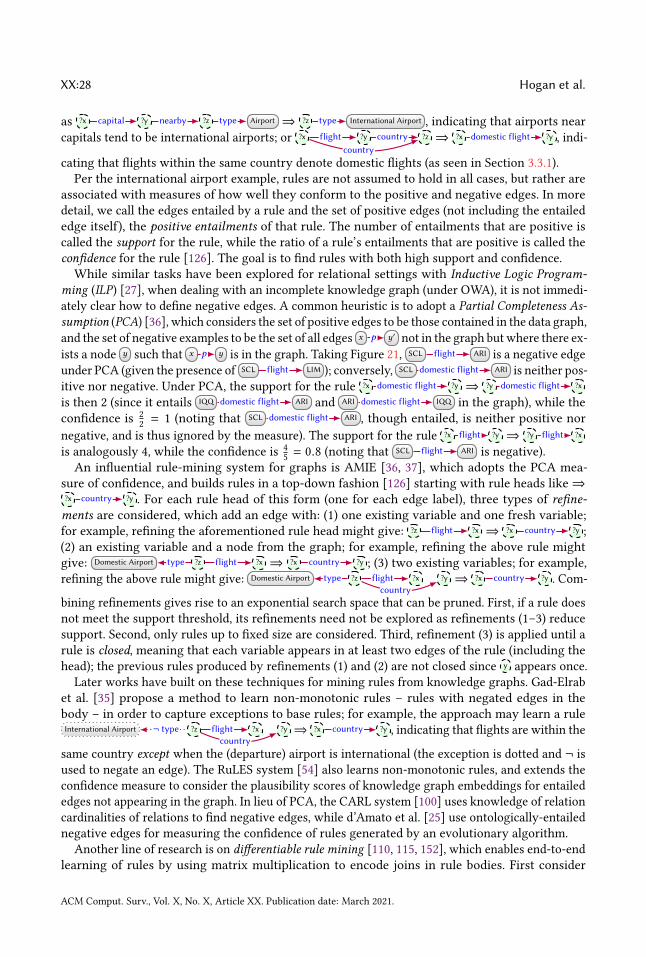
XX:28 Hogan et al.
as ?x ?ycapital ?znearby Airporttype ⇒ ?z International Airporttype , indicating that airports near
capitals tend to be international airports; or ?x ?yflight ?z
countrycountry ⇒ ?x ?ydomestic flight , indi-
cating that flights within the same country denote domestic flights (as seen in Section 3.3.1).
Per the international airport example, rules are not assumed to hold in all cases, but rather are
associated with measures of how well they conform to the positive and negative edges. In more
detail, we call the edges entailed by a rule and the set of positive edges (not including the entailed
edge itself), the positive entailments of that rule. The number of entailments that are positive is
called the support for the rule, while the ratio of a rule’s entailments that are positive is called the
confidence for the rule [126]. The goal is to find rules with both high support and confidence.
While similar tasks have been explored for relational settings with Inductive Logic Program-
ming (ILP) [27], when dealing with an incomplete knowledge graph (under OWA), it is not immedi-
ately clear how to define negative edges. A common heuristic is to adopt a Partial Completeness As-
sumption (PCA) [36], which considers the set of positive edges to be those contained in the data graph,
and the set of negative examples to be the set of all edges x y′p not in the graph but where there ex-
ists a node y such that x yp is in the graph. Taking Figure 21, SCL ARIflight is a negative edge
under PCA (given the presence of SCL LIMflight ); conversely, SCL ARIdomestic flight is neither pos-
itive nor negative. Under PCA, the support for the rule ?x ?ydomestic flight ⇒ ?y ?xdomestic flight
is then 2 (since it entails IQQ ARIdomestic flight and ARI IQQdomestic flight in the graph), while the
confidence is2
2= 1 (noting that SCL ARIdomestic flight , though entailed, is neither positive nor
negative, and is thus ignored by the measure). The support for the rule ?x ?yflight ⇒ ?y ?xflight
is analogously 4, while the confidence is4
5= 0.8 (noting that SCL ARIflight is negative).
An influential rule-mining system for graphs is AMIE [36, 37], which adopts the PCA mea-
sure of confidence, and builds rules in a top-down fashion [126] starting with rule heads like⇒?x ?ycountry . For each rule head of this form (one for each edge label), three types of refine-
ments are considered, which add an edge with: (1) one existing variable and one fresh variable;
for example, refining the aforementioned rule head might give: ?z ?xflight ⇒ ?x ?ycountry ;
(2) an existing variable and a node from the graph; for example, refining the above rule might
give: ?zDomestic Airport type ?xflight ⇒ ?x ?ycountry ; (3) two existing variables; for example,
refining the above rule might give: ?zDomestic Airport type ?xflight ?y
country⇒ ?x ?ycountry . Com-
bining refinements gives rise to an exponential search space that can be pruned. First, if a rule does
not meet the support threshold, its refinements need not be explored as refinements (1–3) reduce
support. Second, only rules up to fixed size are considered. Third, refinement (3) is applied until a
rule is closed, meaning that each variable appears in at least two edges of the rule (including the
head); the previous rules produced by refinements (1) and (2) are not closed since y appears once.
Later works have built on these techniques for mining rules from knowledge graphs. Gad-Elrab
et al. [35] propose a method to learn non-monotonic rules – rules with negated edges in the
body – in order to capture exceptions to base rules; for example, the approach may learn a rule
?zInternational Airport ¬ type ?xflight ?y
country⇒ ?x ?ycountry , indicating that flights are within the
same country except when the (departure) airport is international (the exception is dotted and ¬ is
used to negate an edge). The RuLES system [54] also learns non-monotonic rules, and extends the
confidence measure to consider the plausibility scores of knowledge graph embeddings for entailed
edges not appearing in the graph. In lieu of PCA, the CARL system [100] uses knowledge of relation
cardinalities of relations to find negative edges, while d’Amato et al. [25] use ontologically-entailed
negative edges for measuring the confidence of rules generated by an evolutionary algorithm.
Another line of research is on differentiable rule mining [110, 115, 152], which enables end-to-end
learning of rules by using matrix multiplication to encode joins in rule bodies. First consider
ACM Comput. Surv., Vol. X, No. X, Article XX. Publication date: March 2021.
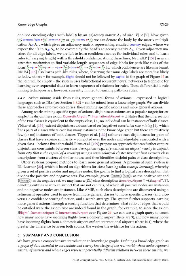
Knowledge Graphs XX:29
one-hot encoding edges with label p by an adjacency matrix Ap of size |V | × |V |. Now given
?x ?ydomestic flight ?zcountry ⇒ ?x ?zcountry , we can denote the body by the matrix multipli-
cation Adf.Ac., which gives an adjacency matrix representing entailed country edges, where we
expect the 1’s in Adf.Ac. to be covered by the head’s adjacency matrix Ac.. Given adjacency ma-
trices for all edge labels, we are left to learn confidence scores for individual rules, and to learn
rules (of varying length) with a threshold confidence. Along these lines, NeuralLP [152] uses an
attention mechanism to find variable-length sequences of edge labels for path-like rules of the
form ?x ?y1p1 . . .p2 ?ynpn ?zpn+1 ⇒ ?x ?zp , for which confidences are likewise learnt.
DRUM [115] also learns path-like rules, where, observing that some edge labels are more/less likely
to follow others – for example, flight should not be followed by capital in the graph of Figure 15 as
the join will be empty – the system uses bidirectional recurrent neural networks (a technique for
learning over sequential data) to learn sequences of relations for rules. These differentiable rule
mining techniques are, however, currently limited to learning path-like rules.
4.4.2 Axiom mining. Aside from rules, more general forms of axioms – expressed in logical
languages such as DLs (see Section 3.3.2) – can be mined from a knowledge graph. We can divide
these approaches into two categories: those mining specific axioms and more general axioms.
Among works mining specific types of axioms, disjointness axioms are a popular target; for ex-
ample, the disjointness axiom DomesticAirport ⊓ InternationalAirport ≡ ⊥ states that the intersection
of the two classes is equivalent to the empty class, i.e., no individual can be instances of both classes.
Völker et al. [136] extract disjointness axioms based on (negative) association rule mining [1], which
finds pairs of classes where each has many instances in the knowledge graph but there are relatively
few (or no) instances of both classes. Töpper et al. [130] rather extract disjointness for pairs of
classes that have a cosine similarity – computed over the nodes and edge-labels associated with a
given class – below a fixed threshold. Rizzo et al. [109] propose an approach that can further capture
disjointness constraints between class descriptions (e.g., city without an airport nearby is disjoint
from city that is the capital of a country) using a terminological cluster tree that first extracts class
descriptions from clusters of similar nodes, and then identifies disjoint pairs of class descriptions.
Other systems propose methods to learn more general axioms. A prominent such system is
DL-Learner [20], which is based on algorithms for class learning (aka concept learning), whereby
given a set of positive nodes and negative nodes, the goal is to find a logical class description that
divides the positive and negative sets. For example, given { Iquique , Arica } as the positive set and
{ Santiago } as the negative set, we may learn a (DL) class description ∃nearby.Airport⊓¬(∃capital−.⊤),denoting entities near to an airport that are not capitals, of which all positive nodes are instances
and no negative nodes are instances. Like AMIE, such class descriptions are discovered using a
refinement operator used to move from more general classes to more specific classes (and vice-
versa), a confidence scoring function, and a search strategy. The system further supports learning
more general axioms through a scoring function that determines what ratio of edges that would
be entailed were the axiom true are indeed found in the graph; for example, to score the axiom
∃flight−.DomesticAirport ⊑ InternationalAirport over Figure 21, we can use a graph query to count
how many nodes have incoming flights from a domestic airport (there are 3), and how many nodes
have incoming flights from a domestic airport and are international airports (there is 1), where the
greater the difference between both counts, the weaker the evidence for the axiom.
5 SUMMARY AND CONCLUSIONWe have given a comprehensive introduction to knowledge graphs. Defining a knowledge graph as
a graph of data intended to accumulate and convey knowledge of the real world, whose nodes represent
entities of interest and whose edges represent potentially different relations between these entities, we
ACM Comput. Surv., Vol. X, No. X, Article XX. Publication date: March 2021.

XX:30 Hogan et al.
have discussed models by which data can be structured, queried and validated as graphs; we also
discussed techniques for leveraging deductive and inductive knowledge over graphs.
Knowledge graphs serve as a common substrate of knowledge within an organisation or com-
munity, enabling the representation, accumulation, curation, and dissemination of knowledge over
time [94]. In this role, knowledge graphs have been applied for diverse use-cases, ranging from
commercial applications – involving semantic search, user recommendations, conversational agents,
targetted advertising, transport automation, etc. – to open knowledge graphs made available for the
public good [56]. General trends include: (1) the use of knowledge graphs to integrate and leverage
data from diverse sources at large scale; and (2) the combination of deductive (rules, ontologies, etc.)
and inductive techniques (machine learning, analytics, etc.) to represent and accumulate knowledge.
Future directions. Research on knowledge graphs can become a confluence of techniques from
different areas with the common objective of maximising the knowledge – and thus value – that
can be distilled from diverse sources at large scale using a graph-based data abstraction.
Particularly interesting topics for knowledge graphs arise from the intersections of areas. In
the intersection of data graphs and deductive knowledge, we emphasise emerging topics such
as formal semantics for property graphs, with languages that can take into account the meaning
of labels and property–value pairs on nodes and edges [73]; and reasoning and querying over
contextual data, in order to derive conclusions and results valid in a particular setting [57, 119, 155].
In the intersection of data graphs and inductive knowledge, we highlight topics such as similarity-
based query relaxation, allowing to find approximate answers to exact queries based on numerical
representations (e.g., embeddings) [138]; shape induction, in order to extract and formalise inherent
patterns in the knowledge graph as constraints [81]; and contextual knowledge graph embeddings that
provide numeric representations of nodes and edges that vary with time, place, etc. [66, 153]. Finally,
in the intersection of deductive and inductive knowledge, we mention the topics of entailment-aware
knowledge graph embeddings [28, 43], that incorporate rules and/or ontologies when computing
plausibility; expressive graph neural networks proven capable of complex classification analogous to
expressive ontology languages [11]; as well as further advances on rule and axiom mining, allowing
to extract symbolic, deductive representations from the knowledge graphs [20, 37].
Aside from specific topics, more general challenges for knowledge graphs include scalability,
particularly for deductive and inductive reasoning; quality, not only in terms of data, but also the
models induced from knowledge graphs; diversity, such as managing contextual or multi-modal
data; dynamicity, considering temporal or streaming data; and finally usability, which is key to
increasing adoption. Though techniques are continuously being proposed to address precisely these
challenges, they are unlikely to ever be completely “solved”; rather they serve as dimensions along
which knowledge graphs, and their techniques, tools, etc., will continue to mature.
Extended version and online material: We refer to the extended version [56] for discussion of further
topics relating to knowledge graphs and formal definitions. We provide concrete examples relating
to the paper in the following repository: https://github.com/knowledge-graphs-tutorial/examples.
Acknowledgements: We thank the organisers and attendees of the Dagstuhl Seminar on “Knowledge
Graphs”, and those who provided feedback on this paper. Hogan was supported by Fondecyt Grant
No. 1181896. Hogan and Gutierrez were funded by ANID – Millennium Science Initiative Program
– Code ICN17_002. Cochez did part of the work while employed at Fraunhofer FIT, Germany and
was later partially funded by Elsevier’s Discovery Lab. Kirrane and Polleres were supported by the
European Union’s Horizon 2020 research and innovation programme under grant 731601. Kirrane,
Ngonga Ngomo, Polleres and Staab received funding through the project “KnowGraphs” from the
European Union’s Horizon programme under the Marie Skłodowska-Curie grant agreement No.
ACM Comput. Surv., Vol. X, No. X, Article XX. Publication date: March 2021.

Knowledge Graphs XX:31
860801. Labra was supported by the Spanish Ministry of Economy and Competitiveness (Society
challenges: TIN2017-88877-R). Navigli was supported by the MOUSSE ERC Grant No. 726487 under
the European Union’s Horizon 2020 research and innovation programme. Rashid was supported by
IBM Research AI through the AI Horizons Network. Schmelzeisen was supported by the German
Research Foundation (DFG) grant STA 572/18-1.
REFERENCES[1] R. Agrawal, T. Imieliński, and A. Swami. 1993. Mining association rules between sets of items in large databases. In
Proc. of SIGMOD.
[2] T. Al-Moslmi, M.G. Ocaña, A.L. Opdahl, and C. Veres. 2020. Named Entity Extraction for Knowledge Graphs: A
Literature Overview. IEEE Access 8 (2020), 32862–32881.
[3] R. Angles. 2018. The Property Graph Database Model. In Proc. of AMW.
[4] R. Angles, M. Arenas, P. Barceló, A. Hogan, J.L. Reutter, and D. Vrgoc. 2017. Foundations of Modern Query Languages
for Graph Databases. ACM Comp. Surveys 50, 5 (2017).
[5] R. Angles, P. Arenas, M. Barceló, P.A. Boncz, G.H.L. Fletcher, C. Gutierrez, T. Lindaaker, M. Paradies, S. Plantikow, J.F.
Sequeda, O. van Rest, and H. Voigt. 2018. G-CORE: A Core for Future Graph Query Languages. In Proc. of SIGMOD.
[6] R. Angles and C. Gutiérrez. 2008. Survey of graph database models. ACM Comp. Surveys 40, 1 (2008).
[7] F. Baader, I. Horrocks, C. Lutz, and U. Sattler. 2017. An Introduction to Description Logic.
[8] I. Balazevic, C. Allen, and M. Hospedales, T. 2019. Hypernetwork Knowledge Graph Embeddings. In Proc. of ICANN
workshops.
[9] I. Balazevic, C. Allen, and T.M. Hospedales. 2019. Multi-relational Poincaré Graph Embeddings. In Proc. of NeurIPs.
[10] I. Balazevic, C. Allen, and T.M. Hospedales. 2019. TuckER: Tensor Factorization for Knowledge Graph Completion. In
Proc. of EMNLP.
[11] P. Barceló, E.V. Kostylev, M. Monet, J. Peréz, J. Reutter, and J.P. Silva. 2020. The Logical Expressiveness of Graph
Neural Networks. In Proc. of ICLR.
[12] L. Bellomarini, E. Sallinger, and G. Gottlob. 2018. The Vadalog System: Datalog-based Reasoning for Knowledge
Graphs. Proc. of the VLDB Endowment 11, 9 (2018).
[13] M.K. Bergman. 2019. A Common Sense View of Knowledge Graphs. Adaptive Information, Adaptive Innovation,
Adaptive Infrastructure Blog. http://www.mkbergman.com/2244/a-common-sense-view-of-knowledge-graphs/.
[14] K. Bollacker, P. Tufts, T. Pierce, and R. Cook. 2007. A platform for scalable, collaborative, structured information
integration. In Intl. Workshop on Information Integration on the Web (IIWeb’07), Ullas Nambiar and Zaiqing Nie (Eds.).
[15] P.A. Bonatti, S. Decker, A. Polleres, and V. Presutti. 2018. Knowledge Graphs: New Directions for Knowledge
Representation on the Semantic Web (Dagstuhl Seminar 18371). Dagstuhl Reports 8, 9 (2018).
[16] P.A. Bonatti, A. Hogan, A. Polleres, and L. Sauro. 2011. Robust and scalable Linked Data reasoning incorporating
provenance and trust annotations. JWS 9, 2 (2011).
[17] A. Bordes, N. Usunier, A. García-Durán, J. Weston, and O. Yakhnenko. 2013. Translating Embeddings for Modeling
Multi-relational Data. In Proc. of NIPS.
[18] D. Brickley and R.V. Guha. 2014. RDF Schema 1.1. W3C Recommendation. W3C.
[19] J. Bruna, W. Zaremba, A. Szlam, and Y. LeCun. 2014. Spectral Networks and Locally Connected Networks on Graphs.
In Proc. of ICLR.
[20] L. Bühmann, J. Lehmann, and P. Westphal. 2016. DL-Learner – A framework for inductive learning on the Semantic
Web. JWS 39 (2016).
[21] Š. Čebirić, F. Goasdoué, H. Kondylakis, D. Kotzinos, I. Manolescu, G. Troullinou, and M. Zneika. 2019. Summarizing
semantic graphs: a survey. VLDB Jour. 28, 3 (2019).
[22] M. Cochez, P. Ristoski, S.P. Ponzetto, and H. Paulheim. 2017. Global RDF Vector Space Embeddings. In Proc. of ISWC
part 1.
[23] S. Cox, C. Little, J.R. Hobbs, and F. Pan. 2017. Time Ontology in OWL. W3C Recommendation / OGC 16-071r2. W3C
and OGC.
[24] R. Cyganiak, D. Wood, and M. Lanthaler. 2014. RDF 1.1 Concepts and Abstract Syntax. W3C Recommendation. W3C.
[25] C. d’Amato, S. Staab, A.G.B. Tettamanzi, D.M. Tran, and F.L. Gandon. 2016. Ontology enrichment by discovering
multi-relational association rules from ontological knowledge bases. In Proc. of SAC.
[26] A. Dave, A. Jindal, L.E. Li, R. Xin, J. Gonzalez, and M. Zaharia. 2016. GraphFrames: an integrated API for mixing
graph and relational queries. In Proc. of GRADES.
[27] L. De Raedt (Ed.). 2008. Logical and Relational Learning: From ILP to MRDM (Cognitive Technologies).
[28] T. Demeester, T. Rocktäschel, and S. Riedel. 2016. Lifted Rule Injection for Relation Embeddings. In Proc. of EMNLP.
ACM Comput. Surv., Vol. X, No. X, Article XX. Publication date: March 2021.
XX:32 Hogan et al.
[29] T. Dettmers, P. Minervini, P. Stenetorp, and S. Riedel. 2018. Convolutional 2D Knowledge Graph Embeddings. In Proc.
of AAAI.
[30] R.Q. Dividino, S. Sizov, S. Staab, and B. Schueler. 2009. Querying for provenance, trust, uncertainty and other meta
knowledge in RDF. JWS 7, 3 (2009).
[31] X. Dong, E. Gabrilovich, G. Heitz, W. Horn, N. Lao, K. Murphy, T. Strohmann, S. Sun, and W. Zhang. 2014. Knowledge
vault: a web-scale approach to probabilistic knowledge fusion. In Proc. of KDD.
[32] L. Ehrlinger and W. Wöß. 2016. Towards a Definition of Knowledge Graphs. In Proc. of SEMANTiCS posters & demos.
[33] D. Fensel, U. Simsek, K. Angele, E. Huaman, E. Kärle, O. Panasiuk, I. Toma, J. Umbrich, and A. Wahler. 2020. Knowledge
Graphs - Methodology, Tools and Selected Use Cases. Springer.
[34] N. Francis, A. Green, P. Guagliardo, L. Libkin, T. Lindaaker, V. Marsault, S. Plantikow, M. Rydberg, P. Selmer, and A.
Taylor. 2018. Cypher: An Evolving Query Language for Property Graphs. In Proc. of SIGMOD.
[35] M.H. Gad-Elrab, D. Stepanova, J. Urbani, and G. Weikum. 2016. Exception-Enriched Rule Learning from Knowledge
Graphs. In Proc. of ISWC part 1.
[36] L.A. Galárraga, C. Teflioudi, K. Hose, and F. Suchanek. 2013. AMIE: association rule mining under incomplete evidence
in ontological knowledge bases. In Proc. of WWW.
[37] L. Galárraga, C. Teflioudi, K. Hose, and F.M. Suchanek. 2015. Fast rule mining in ontological knowledge bases with
AMIE+. VLDB Jour. 24, 6 (2015).
[38] G.A. Gesese, R. Biswas, and Sack H. 2019. A Comprehensive Survey of Knowledge Graph Embeddings with Literals:
Techniques and Applications. In Proc. of DL4KG.
[39] Y. Gil, S. Miles, K. Belhajjame, D. Garijo, G. Klyne, P. Missier, S. Soiland-Reyes, and S. Zednik. 2013. PROV Model
Primer. W3C Working Group Note. W3C.
[40] J.M. Giménez-García, A. Zimmermann, and P. Maret. 2017. NdFluents: An Ontology for Annotated Statements with
Inference Preservation. In Proc. of ESWC part 1.
[41] X. Glorot, A. Bordes, J. Weston, and Y. Bengio. 2013. A Semantic Matching Energy Function for Learning with
Multi-relational Data. In Proc. of ICLR workshops.
[42] R.V. Guha, R. McCool, and R. Fikes. 2004. Contexts for the Semantic Web. In Proc. of ISWC.
[43] S. Guo, Q. Wang, L. Wang, B. Wang, and L. Guo. 2016. Jointly Embedding Knowledge Graphs and Logical Rules. In
Proc. of EMNLP.
[44] C. Gutiérrez, C.A. Hurtado, and A.A. Vaisman. 2007. Introducing Time into RDF. IEEE Trans. on Know. & Data Eng.
19, 2 (2007).
[45] W. L. Hamilton, P. Bajaj, M. Zitnik, D. Jurafsky, and J. Leskovec. 2018. Embedding Logical Queries on Knowledge
Graphs. In Proc. of NIPS.
[46] S. Harris, A. Seaborne, and E. Prud’hommeaux. 2013. SPARQL 1.1 Query Language. W3C Recommendation. W3C.
[47] O. Hartig. 2017. Foundations of RDF* and SPARQL* – An Alternative Approach to Statement-Level Metadata in RDF.
In Proc. of AMW.
[48] T. Heath and C. Bizer. 2011. Linked Data: Evolving the Web into a Global Data Space (1st Edition). Vol. 1.
[49] N. Heist, S. Hertling, R. Ringler, and H. Paulheim. 2020. Knowledge Graphs on the Web – an Overview. CoRR
abs/2003.00719 (2020). https://arxiv.org/abs/2003.00719
[50] D. Hernández, A. Hogan, and M. Krötzsch. 2015. Reifying RDF: What Works Well With Wikidata?. In Proc. of SSWS.
[51] F.L. Hitchcock. 1927. The Expression of a Tensor or a Polyadic as a Sum of Products. Jour. of Math. & Physics 6, 1–4
(1927).
[52] P. Hitzler, M. Krötzsch, B. Parsia, P.F. Patel-Schneider, and S. Rudolph. 2012. OWL 2 Web Ontology Language Primer
(Second Edition). W3C Recommendation. W3C.
[53] P. Hitzler, M. Krötzsch, and S. Rudolph. 2010. Foundations of Semantic Web Technologies.
[54] V.T. Ho, D. Stepanova, M.H. Gad-Elrab, E. Kharlamov, and G. Weikum. 2018. Rule Learning from Knowledge Graphs
Guided by Embedding Models. In Proc. of ISWC part 1.
[55] J. Hoffart, F.M. Suchanek, K. Berberich, E. Lewis-Kelham, G. de Melo, and G. Weikum. 2011. YAGO2: Exploring and
Querying World Knowledge in Time, Space, Context, and Many Languages. In Proc. of WWW companion volume.
[56] A. Hogan, E. Blomqvist, M. Cochez, C. d’Amato, G. de Melo, C. Gutierrez, J.E. Labra Gayo, S. Kirrane, S. Neumaier,
A. Polleres, R. Navigli, A.C. Ngonga Ngomo, S.M. Rashid, A. Rula, L. Schmelzeisen, J.F. Sequeda, S. Staab, and A.
Zimmermann. 2020. Knowledge Graphs. CoRR (2020). arXiv:2003.02320 https://arxiv.org/abs/2003.02320
[57] M. Homola and L. Serafini. 2012. Contextualized Knowledge Repositories for the Semantic Web. JWS 12 (2012).
[58] I. Horrocks, P.F. Patel-Schneider, H. Boley, S. Tabet, B. Grosof, and M. Dean. 2004. SWRL: A Semantic Web Rule
Language Combining OWL and RuleML. W3C Member Submission.
[59] x. Huang, J. Zhang, D. Li, and P. Li. 2019. Knowledge Graph Embedding Based Question Answering. In Proc. of
WSDM.
ACM Comput. Surv., Vol. X, No. X, Article XX. Publication date: March 2021.
Knowledge Graphs XX:33
[60] R. Hussein, D. Yang, and P. Cudré-Mauroux. 2018. Are Meta-Paths Necessary?: Revisiting Heterogeneous Graph
Embeddings.
[61] A. Iosup, T. Hegeman, W.L. Ngai, S. Heldens, A. Prat-Pérez, T. Manhardt, H. Chafi, M. Capota, N. Sundaram, M.J.
Anderson, I.G. Tanase, Y. Xia, L. Nai, and P.A. Boncz. 2016. LDBC Graphalytics: A Benchmark for Large-Scale Graph
on Parallel and Distributed Platforms. Proc. of the VLDB Endowment 9, 13 (2016).
[62] D. Janke and S. Staab. 2018. Storing and Querying Semantic Data in the Cloud. In Proc. of RW.
[63] G. Ji, S. He, L. Xu, K. Liu, and J. Zhao. 2015. Knowledge graph embedding via dynamic mapping matrix. In Proc. of
ACL part 1.
[64] S. Ji, S. Pan, E. Cambria, P. Marttinen, and P.S. Yu. 2020. A Survey on Knowledge Graphs: Representation, Acquisition
and Applications. CoRR abs/2002.00388 (2020).
[65] E. Kärle, U. Simsek, O. Panasiuk, and D. Fensel. 2018. Building an Ecosystem for the Tyrolean Tourism Knowledge
Graph. CoRR abs/1805.05744 (2018).
[66] S.M. Kazemi, R. Goel, K. Jain, I. Kobyzev, A. Sethi, P. Forsyth, and P. Poupart. 2019. Relational Representation Learning
for Dynamic (Knowledge) Graphs: A Survey. CoRR abs/1905.11485 (2019).
[67] S.M. Kazemi and D. Poole. 2018. SimplE Embedding for Link Prediction in Knowledge Graphs. In Proc. of NIPS.
[68] M. Kejriwal. 2019. Domain-Specific Knowledge Graph Construction. Springer.
[69] M. Kifer and H. Boley. 2013. RIF Overview (Second Edition). W3C Working Group Note. W3C.
[70] T.N. Kipf and M. Welling. 2017. Semi-Supervised Classification with Graph Convolutional Networks. In Proc. of ICLR.
[71] H. Knublauch and D. Kontokostas. 2017. Shapes Constraint Language (SHACL). W3C Recommendation. W3C.
[72] A. Krizhevsky, I. Sutskever, and G.E. Hinton. 2017. ImageNet classification with deep convolutional neural networks.
ACM Comm. 60, 6 (2017).
[73] M. Krötzsch, M. Marx, A. Ozaki, and V. Thost. 2018. Attributed Description Logics: Reasoning on Knowledge Graphs.
In Proc. of IJCAI.
[74] J.E. Labra Gayo, E. Prud’hommeaux, I. Boneva, and D. Kontokostas. 2017. Validating RDF Data. Vol. 7.
[75] J. Lehmann, R. Isele, M. Jakob, A. Jentzsch, D. Kontokostas, P.N. Mendes, S. Hellmann, M. Morsey, P. van Kleef, S.
Auer, and C. Bizer. 2015. DBpedia - A large-scale, multilingual knowledge base extracted from Wikipedia. SWJ 6, 2
(2015).
[76] Y. Lin, Z. Liu, M. Sun, Y. Liu, and X. Zhu. 2015. Learning entity and relation embeddings for knowledge graph
completion. In Proc. of AAAI.
[77] Y. Low, J. Gonzalez, A. Kyrola, D. Bickson, C. Guestrin, and J.M. Hellerstein. 2012. Distributed GraphLab: A Framework
for Machine Learning in the Cloud. Proc. of the VLDB Endowment 5, 8 (2012).
[78] C. Lu, P. Laublet, and M. Stankovic. 2016. Travel Attractions Recommendation with Knowledge Graphs. In Proc. of
EKAW.
[79] G. Malewicz, M.H. Austern, A.J.C. Bik, J.C. Dehnert, I. Horn, N. Leiser, and G. Czajkowski. 2010. Pregel: a system for
large-scale graph processing. In Proc. of SIGMOD.
[80] J. McCarthy. 1993. Notes on Formalizing Context. In Proc. of IJCAI.
[81] N. Mihindukulasooriya, M. Rashid, G. Rizzo, R. García-Castro, Ó. Corcho, and M. Torchiano. 2018. RDF shape
induction using knowledge base profiling. In Proc. of SAC.
[82] T. Mikolov, K. Chen, G. Corrado, and J. Dean. 2013. Efficient estimation of word representations in vector space. In
Proc. of ICLR workshops. arXiv preprint arXiv:1301.3781.
[83] J.J. Miller. 2013. Graph Database Applications and Concepts with Neo4j. In Proceedings of the Southern Association for
Information Systems Conference, Atlanta, GA, USA March 23rd-24th, 2013. Article 24.
[84] M. Minsky. 1974. A Framework for representing knowledge. MIT-AI Memo 306, Santa Monica (1974).
[85] F. Monti, D. Boscaini, J. Masci, E. Rodolà, J. Svoboda, and M.M. Bronstein. 2017. Geometric Deep Learning on Graphs
and Manifolds Using Mixture Model CNNs. In Proc. of CVPR.
[86] B. Motik, B.C. Grau, I. Horrocks, Z. Wu, A. Fokoue, and C. Lutz. 2012. OWL 2 Web Ontology Language Profiles (Second
Edition). W3C Recommendation. W3C.
[87] B. Motik, R. Shearer, and I. Horrocks. 2009. Hypertableau Reasoning for Description Logics. JAIR 36 (2009).
[88] C. Mungall, A. Ruttenberg, I. Horrocks, and D. Osumi-Sutherland. 2012. OBO Flat File Format 1.4 Syntax and Semantics.
Editor’s Draft.
[89] R. Navigli and S.P. Ponzetto. 2012. BabelNet: The automatic construction, evaluation and application of a wide-coverage
multilingual semantic network. AI Jour. 193 (2012).
[90] V. Nguyen, O. Bodenreider, and A. Sheth. 2014. Don’t Like RDF Reification?: Making Statements About Statements
Using Singleton Property. In Proc. of WWW.
[91] M. Nickel, L. Rosasco, and T.A. Poggio. 2016. Holographic Embeddings of Knowledge Graphs. In Proc. of AAAI.
[92] M. Nickel and V. Tresp. 2013. Tensor factorization for multi-relational learning. In Proc. of ECML-PKDD part 3.
[93] I. Nonaka and H. Takeuchi. 1995. The Knowledge-Creating Company. Oxford Uni.
ACM Comput. Surv., Vol. X, No. X, Article XX. Publication date: March 2021.

XX:34 Hogan et al.
[94] N.F. Noy, Y. Gao, A. Jain, A. Narayanan, A. Patterson, and J. Taylor. 2019. Industry-scale Knowledge Graphs: Lessons
and Challenges. ACM Queue 17, 2 (2019).
[95] L. Page, S. Brin, R. Motwani, and T. Winograd. 1999. The PageRank Citation Ranking: Bringing order to the Web.
Technical Report 1999-66. Stanford InfoLab.
[96] J.Z. Pan, G. Vetere, Gómez-Pérez J.M., and H. Wu (Eds.). 2017. Exploiting Linked Data and Knowledge Graphs in Large
Organisations. Springer.
[97] N. Park, A. Kan, X.L. Dong, T. Zhao, and C. Faloutsos. 2019. Estimating Node Importance in Knowledge Graphs Using
Graph Neural Networks. In Proc. of SIGKDD.
[98] N. Park, A. Kan, X.L. Dong, T. Zhao, and C. Faloutsos. 2020. MultiImport: Inferring Node Importance in a Knowledge
Graph from Multiple Input Signals. In Proc. of SIGKDD.
[99] H. Paulheim. 2017. Knowledge graph refinement: A survey of approaches and evaluation methods. SWJ 8, 3 (2017).
[100] T. Pellissier Tanon, D. Stepanova, S. Razniewski, P. Mirza, and G. Weikum. 2017. Completeness-Aware Rule Learning
from Knowledge Graphs. In Proc. of ISWC part 1.
[101] J. Pennington, R. Socher, and C. Manning. 2014. Glove: Global vectors for word representation. In Proc. of EMNLP.
[102] A. Piscopo, L. Kaffee, C. Phethean, and E. Simperl. 2017. Provenance Information in a Collaborative Knowledge
Graph: An Evaluation of Wikidata External References. In Proc. of ISWC part 1.
[103] E. Prud’hommeaux, J.E. Labra Gayo, and H. Solbrig. 2014. Shape Expressions: An RDF Validation and Transformation
Language. In Proc. of SEMANTICS.
[104] J. Pujara, H. Miao, L. Getoor, and W.W. Cohen. 2013. Knowledge Graph Identification. In Proc. of ISWC part 1.
[105] G. Qi, H. Chen, K. Liu, H. Wang, Q. Ji, and T. Wu. 2020. Knowledge Graph. (To appear).
[106] R. Quillian. 1963. A notation for representing conceptual information: An application to semantics and mechanical
English paraphrasing. Technical Report SP-1395. Systems Development Corp.
[107] S. Rabanser, O. Shchur, and S. Günnemann. 2017. Introduction to Tensor Decompositions and their Applications in
Machine Learning. CoRR abs/1711.10781 (2017). arXiv:1711.10781
[108] P. Ristoski and H. Paulheim. 2016. RDF2Vec: RDF Graph Embeddings for Data Mining. In Proc. of ISWC part 1.
[109] G. Rizzo, C. d’Amato, N. Fanizzi, and F. Esposito. 2017. Terminological Cluster Trees for Disjointness Axiom Discovery.
In Proc. of ESWC part 1.
[110] T. Rocktäschel and S. Riedel. 2017. End-to-end Differentiable Proving. In Proc. of NIPS.
[111] M.A. Rodriguez. 2015. The Gremlin graph traversal machine and language. In Proc. of DBPL.
[112] S. Rudolph, M. Krötzsch, and P. Hitzler. 2008. Description Logic Reasoning with Decision Diagrams: Compiling SHIQ
to Disjunctive Datalog. In Proc. of ISWC.
[113] A. Rula, M. Palmonari, A. Harth, S. Stadtmüller, and A. Maurino. 2012. On the Diversity and Availability of Temporal
Information in Linked Open Data. In Proc. of ISWC part 1.
[114] A. Rula, M. Palmonari, S. Rubinacci, A. Ngonga Ngomo, J. Lehmann, A. Maurino, and D. Esteves. 2019. TISCO:
Temporal scoping of facts. JWS 54 (2019).
[115] A. Sadeghian, M. Armandpour, P. Ding, and P. Wang. 2019. DRUM: End-To-End Differentiable Rule Mining On
Knowledge Graphs. In Proc. of NIPS.
[116] F. Scarselli, M. Gori, A.C. Tsoi, M. Hagenbuchner, and G. Monfardini. 2009. The Graph Neural Network Model. IEEE
Trans. on Neur. Net. 20, 1 (2009).
[117] E.W. Schneider. 1973. Course Modularization Applied: The Interface System and Its Implications For Sequence Control
and Data Analysis. In Association for the Development of Instructional Systems (ADIS), Chicago, Illinois, April 1972.
[118] M. Schneider and G. Sutcliffe. 2011. Reasoning in the OWL 2 Full Ontology Language Using First-Order Automated
Theorem Proving. In Proc. of CADE.
[119] C. Schuetz, L. Bozzato, B. Neumayr, M. Schrefl, and L. Serafini. 2020. Knowledge Graph OLAP: A Multidimensional
Model and Query Operations for Contextualized Knowledge Graphs. SWJ (2020). (Under open review).
[120] P. Seifer, J. Härtel, M. Leinberger, R. Lämmel, and S. Staab. 2019. Empirical study on the usage of graph query
languages in open source Java projects. In Proc. of SLE.
[121] A. Singhal. 2012. Introducing the Knowledge Graph: things, not strings. Google Blog. https://www.blog.google/
products/search/introducing-knowledge-graph-things-not/.
[122] R. Socher, D. Chen, C.D. Manning, and A. Ng. 2013. Reasoning with neural tensor networks for knowledge base
completion. In Proc. of NIPS.
[123] A. Sperduti and A. Starita. 1997. Supervised neural networks for the classification of structures. IEEE Trans. on Neur.
Net. 8, 3 (1997).
[124] U. Straccia. 2009. A Minimal Deductive System for General Fuzzy RDF. In Proc. of RR.
[125] P. Stutz, D. Strebel, and A. Bernstein. 2016. Signal/Collect12. SWJ 7, 2 (2016).
[126] F.M. Suchanek, J. Lajus, A. Boschin, and G. Weikum. 2019. Knowledge Representation and Rule Mining in Entity-
Centric Knowledge Bases. In Proc. of RWeb.
ACM Comput. Surv., Vol. X, No. X, Article XX. Publication date: March 2021.

Knowledge Graphs XX:35
[127] Yizhou Sun and Jiawei Han. 2012. Mining Heterogeneous Information Networks: Principles and Methodologies. Morgan
& Claypool Publishers.
[128] Y. Sun, J. Han, X. Yan, P.S. Yu, and T. Wu. 2011. Pathsim: Meta path-based top-k similarity search in heterogeneous
information networks. Proc. of the VLDB Endowment 4, 11 (2011).
[129] Z. Sun, Z. Deng, J. Nie, and J. Tang. 2019. RotatE: Knowledge Graph Embedding by Relational Rotation in Complex
Space. In Proc. of ICLR.
[130] G. Töpper, M. Knuth, and H. Sack. 2012. DBpedia ontology enrichment for inconsistency detection. In Proc. of
I-SEMANTICS.
[131] T. Trouillon, J. Welbl, S. Riedel, É. Gaussier, and G. Bouchard. 2016. Complex Embeddings for Simple Link Prediction.
In Proc. of ICML.
[132] L.R. Tucker. 1964. The extension of factor analysis to three-dimensional matrices. In Contributions to Mathematical
Psychology.
[133] O. Udrea, D. Reforgiato Recupero, and V.S. Subrahmanian. 2010. Annotated RDF. ACM Trans. on Comp. Log. 11, 2
(2010).
[134] S. Vashishth, P. Jain, and P. Talukdar. 2018. CESI: Canonicalizing Open Knowledge Bases using Embeddings and Side
Information. In Proc. of WWW.
[135] P. Velickovic, G. Cucurull, A. Casanova, A. Romero, P. Liò, and Y. Bengio. 2018. Graph Attention Networks. In Proc. of
ICLR.
[136] J. Völker, D. Fleischhacker, and H. Stuckenschmidt. 2015. Automatic Acquisition of Class Disjointness. JWS 35, P2
(2015).
[137] D. Vrandečić and M. Krötzsch. 2014. Wikidata: A Free Collaborative Knowledgebase. ACM Comm. 57, 10 (2014).
[138] M. Wang, R. Wang, J. Liu, Y. Chen, L. Zhang, and G. Qi. 2018. Towards Empty Answers in SPARQL: Approximating
Querying with RDF Embedding. In Proc. of ISWC.
[139] Q. Wang, Z. Mao, B. Wang, and L. Guo. 2017. Knowledge Graph Embedding: A Survey of Approaches and Applications.
IEEE Trans. on Know. & Data Eng. 29, 12 (Dec. 2017).
[140] Q. Wang, B. Wang, and L. Guo. 2015. Knowledge Base Completion Using Embeddings and Rules. In Proc. of IJCAI.
[141] X. Wang, H. Ji, C. Shi, B. Wang, Y. Ye, P. Cui, and P.S. Yu. 2019. Heterogeneous Graph Attention Network. In Proc. of
WWW.
[142] X. Wang and S. Yang. 2019. A Tutorial and Survey on Fault Knowledge Graph. In Proc. of CyberDI/CyberLife. 256–271.
[143] Z. Wang, J. Zhang, J. Feng, and Z. Chen. 2014. Knowledge Graph Embedding by Translating on Hyperplanes. In Proc.
of AAAI.
[144] Z. Wu, S. Pan, F. Chen, G. Long, C. Zhang, and P.S. Yu. 2019. A Comprehensive Survey on Graph Neural Networks.
CoRR abs/1901.00596 (2019).
[145] Marcin Wylot, Manfred Hauswirth, Philippe Cudré-Mauroux, and Sherif Sakr. 2018. RDF Data Storage and Query
Processing Schemes: A Survey. ACM Comp. Surveys 51, 4 (2018).
[146] G. Xiao, L. Ding, G. Cogrel, and D. Calvanese. 2019. Virtual Knowledge Graphs: An Overview of Systems and Use
Cases. Data Int. 1, 3 (2019), 201–223.
[147] R. Xin, J. Gonzalez, M.J. Franklin, and I. Stoica. 2013. GraphX: a resilient distributed graph system on Spark. In Proc.
of GRADES.
[148] R. Xin, J. Rosen, M. Zaharia, M.J. Franklin, S. Shenker, and I. Stoica. 2013. Shark: SQL and rich analytics at scale. In
Proc. of SIGMOD.
[149] K. Xu, W. Hu, J. Leskovec, and S. Jegelka. 2019. How Powerful are Graph Neural Networks?. In Proc. of ICLR.
[150] J. Yan, C. Wang, W. Cheng, M. Gao, and A. Zhou. 2018. A retrospective of knowledge graphs. Frontiers C.S. 12, 1
(2018), 55–74.
[151] B. Yang, W. Yih, X. He, J. Gao, and L. Deng. 2015. Embedding Entities and Relations for Learning and Inference in
Knowledge Bases. In Proc. of ICLR.
[152] F. Yang, Z. Yang, and W.W. Cohen. 2017. Differentiable Learning of Logical Rules for Knowledge Base Reasoning. In
Proc. of NIPS.
[153] L. Yang, Z. Xiao, W. Jiang, Y. Wei, Y. Hu, and H. Wang. 2020. Dynamic Heterogeneous Graph Embedding Using
Hierarchical Attentions. In Proc. of ECIR.
[154] F. Zhang, N.J. Yuan, D. Lian, X. Xie, and W. Ma. 2016. Collaborative knowledge base embedding for recommender
systems. In Proc. of SIGKDD.
[155] A. Zimmermann, N. Lopes, A. Polleres, and U. Straccia. 2012. A General Framework for Representing, Reasoning and
Querying with Annotated Semantic Web Data. JWS 12 (mar 2012).
ACM Comput. Surv., Vol. X, No. X, Article XX. Publication date: March 2021.
Copyright © 2022 FDOKUMEN


![arXiv:1912.05704v1 [astro-ph.HE] 12 Dec 2019 - ePrints Soton](https://static.fdokumen.com/doc/165x107/631962ea1a1adcf65a0ea184/arxiv191205704v1-astro-phhe-12-dec-2019-eprints-soton.jpg)