
Dynamic Cost Modelling Through Factory Simulation - ePrints Soton
294
UNIVERSITY OF SOUTHAMPTON FACULTY OF ENGINEERING AND THE ENVIRONMENT Computational Engineering and Design Group The use of automated process planning to minimise unit cost whilst retaining flexibility of manufacturing method by David Cooper MEng Thesis for the degree of Engineering Doctorate August 2016
-
Upload
khangminh22 -
Category
Documents
-
view
1 -
download
0
Transcript of Dynamic Cost Modelling Through Factory Simulation - ePrints Soton
UNIVERSITY OF SOUTHAMPTON
FACULTY OF ENGINEERING AND THE ENVIRONMENT
Computational Engineering and Design Group
The use of automated process planning to minimise unit cost whilst retainingflexibility of manufacturing method
by
David Cooper MEng
Thesis for the degree of Engineering Doctorate
August 2016


UNIVERSITY OF SOUTHAMPTON
ABSTRACT
FACULTY OF ENGINEERING AND THE ENVIRONMENT
Computational Engineering and Design Group
Thesis for the degree of Engineering Doctorate
THE USE OF AUTOMATED PROCESS PLANNING TO MINIMISE UNITCOST WHILST RETAINING FLEXIBILITY OF MANUFACTURING
METHOD
by David Stephen Cooper
This research focussed on the automatic generation of the optimal method of manufacture,and the cost thereof, at an early stage in design. It used geometric and tolerance data,combined with a database of centrally stored manufacturing knowledge. This allowed theconstruction of potential manufacturing routes, and the evaluation of their cost.
In order to find the least costly method of manufacture for a given component, withdefined geometry and tolerance, it is necessary to take a holistic view of the manufacturingprocess. This thesis shows that the typical sequential approach of choosing themanufacturing process, followed by sequencing, will not necessarily find the globaloptimum. Dynamic process seletion is required to consider both the choice ofmanufacturing processes and the sequence together to avoid sub-optimisation.
Backward and forward propagation from a final manufacturing process, using a randommutation hill climber, was used to construct potential manufacturing process sets. For eachprocess set constructed, the inner optimisation loop was used to find the optimal sequenceof manufacturing operations, with the aid of a repair operator to ensure feasibility.
Prior to finding the optimal manufacturing sequence, the forming shape for all potentialforming processes was required; this research encompasses a methodology to automaticallydeduce this shape.
This methodology demonstrated convergence to the global optimum on a contrived testcase, and has demonstrated accurate results on a real commercial test case. Major areas forimprovement could be a combination of the developed methodology with featurerecognition, to enable maximum usefulness as a fully automated process planning and costevaluation tool.
In summary this research demonstrates that the lack of a holistic view can causesub-optimal results, and proposes a methodology which provides a holistic perspective.The methodology has been proved to be accurate, generic and expandable.

Contents
1 Introduction 1
1.1 Research Introduction . . . . . . . . . . . . . . . . . . . . . . . . . . . . . . . 1
1.2 Hypothesis . . . . . . . . . . . . . . . . . . . . . . . . . . . . . . . . . . . . . 2
1.3 Objective . . . . . . . . . . . . . . . . . . . . . . . . . . . . . . . . . . . . . . 2
1.3.1 Sub-objectives . . . . . . . . . . . . . . . . . . . . . . . . . . . . . . . 3
1.4 Vision . . . . . . . . . . . . . . . . . . . . . . . . . . . . . . . . . . . . . . . . 4
1.5 Overall Architecture . . . . . . . . . . . . . . . . . . . . . . . . . . . . . . . . 5
1.6 Methodology structure and interfaces . . . . . . . . . . . . . . . . . . . . . . . 9
1.6.1 Software . . . . . . . . . . . . . . . . . . . . . . . . . . . . . . . . . . . 10
1.6.2 Created Tools . . . . . . . . . . . . . . . . . . . . . . . . . . . . . . . . 11
1.6.3 The component model and spreadsheet . . . . . . . . . . . . . . . . . 11
1.7 Industrial sponsor context . . . . . . . . . . . . . . . . . . . . . . . . . . . . . 13
1.7.1 The Front Bearing Housing (FBH) . . . . . . . . . . . . . . . . . . . . 13
1.7.2 Feature Classification and standard features . . . . . . . . . . . . . . . 13
1.7.3 Model Construction Data . . . . . . . . . . . . . . . . . . . . . . . . . 18
1.7.4 Manufacturing knowledge . . . . . . . . . . . . . . . . . . . . . . . . . 18
1.7.5 Verification/Validation Data . . . . . . . . . . . . . . . . . . . . . . . 21
1.8 Test Cases . . . . . . . . . . . . . . . . . . . . . . . . . . . . . . . . . . . . . . 23
1.8.1 Minor Test Cases . . . . . . . . . . . . . . . . . . . . . . . . . . . . . . 26
1.9 Papers and patents . . . . . . . . . . . . . . . . . . . . . . . . . . . . . . . . . 28
1.10 Thesis synopsis . . . . . . . . . . . . . . . . . . . . . . . . . . . . . . . . . . . 28
2 Literature Survey 31
2.1 The Design Process . . . . . . . . . . . . . . . . . . . . . . . . . . . . . . . . . 31
2.1.1 Concurrent vs Iterative Loop Engineering . . . . . . . . . . . . . . . . 33

2.1.2 Potential Design Methods . . . . . . . . . . . . . . . . . . . . . . . . . 35
2.1.3 Features . . . . . . . . . . . . . . . . . . . . . . . . . . . . . . . . . . . 36
2.1.4 Feature Recognition . . . . . . . . . . . . . . . . . . . . . . . . . . . . 38
2.1.5 Design for Manufacture Systems . . . . . . . . . . . . . . . . . . . . . 45
2.1.6 Value Driven Design (VDD) . . . . . . . . . . . . . . . . . . . . . . . . 50
2.1.7 Summary of the design process . . . . . . . . . . . . . . . . . . . . . . 51
2.2 Process Planning . . . . . . . . . . . . . . . . . . . . . . . . . . . . . . . . . . 52
2.2.1 Supply chain modelling . . . . . . . . . . . . . . . . . . . . . . . . . . 53
2.2.2 An Introduction to CAPP (Computer Aided Process Planning) . . . . 54
2.2.3 Knowledge Representation . . . . . . . . . . . . . . . . . . . . . . . . . 57
2.2.4 A Review of CAPP Methods . . . . . . . . . . . . . . . . . . . . . . . 57
2.2.5 CAPP methods: Variant Method . . . . . . . . . . . . . . . . . . . . . 60
2.2.6 CAPP methods: Infeasible solutions . . . . . . . . . . . . . . . . . . . 62
2.2.7 CAPP methods: Genetic Algorithm . . . . . . . . . . . . . . . . . . . 62
2.2.8 CAPP Methods: Graphical Algorithms . . . . . . . . . . . . . . . . . 65
2.2.9 CAPP Methods: Simulated Annealing . . . . . . . . . . . . . . . . . . 65
2.2.10 CAPP Methods: ANN (Artificial Neural Network) . . . . . . . . . . . 66
2.2.11 CAPP Methods: Logic and Query based . . . . . . . . . . . . . . . . . 67
2.2.12 CAPP Methods: Other . . . . . . . . . . . . . . . . . . . . . . . . . . 67
2.2.13 Difficulties with CAPP . . . . . . . . . . . . . . . . . . . . . . . . . . . 68
2.2.14 ASP (Assembly Sequence Planning) . . . . . . . . . . . . . . . . . . . 69
2.2.15 Process selection and sequencing . . . . . . . . . . . . . . . . . . . . . 70
2.2.16 Production planning (Scheduling) . . . . . . . . . . . . . . . . . . . . 70
2.2.17 Summary of process planning . . . . . . . . . . . . . . . . . . . . . . . 71
2.3 Integrating CAPP with CAD . . . . . . . . . . . . . . . . . . . . . . . . . . . 73

2.3.1 Summary of CAD-CAPP integration . . . . . . . . . . . . . . . . . . . 76
2.4 Prediction of precursor shape . . . . . . . . . . . . . . . . . . . . . . . . . . . 77
2.5 Manufacturing Processes . . . . . . . . . . . . . . . . . . . . . . . . . . . . . . 80
2.5.1 Material Removal . . . . . . . . . . . . . . . . . . . . . . . . . . . . . . 80
2.5.2 Joining (Welding) . . . . . . . . . . . . . . . . . . . . . . . . . . . . . 82
2.5.3 Manufacturing processes modelling and optimisation . . . . . . . . . . 82
2.5.4 Fixturing . . . . . . . . . . . . . . . . . . . . . . . . . . . . . . . . . . 83
2.5.5 Summary of manufacturing processes . . . . . . . . . . . . . . . . . . . 84
2.6 Cost Modelling . . . . . . . . . . . . . . . . . . . . . . . . . . . . . . . . . . . 85
2.6.1 Parametric Cost Modelling in Early Design . . . . . . . . . . . . . . . 86
2.6.2 Parametric cost modelling in detailed design . . . . . . . . . . . . . . 87
2.6.3 Generative Cost modelling . . . . . . . . . . . . . . . . . . . . . . . . . 87
2.6.4 Creation of Cost Models . . . . . . . . . . . . . . . . . . . . . . . . . . 89
2.6.5 Cost rates for machinery . . . . . . . . . . . . . . . . . . . . . . . . . 90
2.6.6 Using CAM Data for Cost Model Improvement . . . . . . . . . . . . . 91
2.6.7 Summary of cost modelling . . . . . . . . . . . . . . . . . . . . . . . . 93
2.7 Summary of Literature Review . . . . . . . . . . . . . . . . . . . . . . . . . . 94
3 Commercial Costing Systems 95
3.1 Internal Methodologies of Industrial Sponsor . . . . . . . . . . . . . . . . . . 95
3.2 aPriori . . . . . . . . . . . . . . . . . . . . . . . . . . . . . . . . . . . . . . . . 95
3.2.1 Selection of manufacturing strategy . . . . . . . . . . . . . . . . . . . 96
3.2.2 The aPriori Virtual Production Environment (VPE) . . . . . . . . . . 96
3.2.3 Selection of manufacturing processes . . . . . . . . . . . . . . . . . . . 97
3.2.4 Selection of machines . . . . . . . . . . . . . . . . . . . . . . . . . . . 97
3.2.5 Cost Modelling . . . . . . . . . . . . . . . . . . . . . . . . . . . . . . . 98

3.2.6 Assemblies . . . . . . . . . . . . . . . . . . . . . . . . . . . . . . . . . 98
3.2.7 Summary of aPriori . . . . . . . . . . . . . . . . . . . . . . . . . . . . 98
3.3 Perfect Costing (Siemens) . . . . . . . . . . . . . . . . . . . . . . . . . . . . . 99
3.4 CATIA . . . . . . . . . . . . . . . . . . . . . . . . . . . . . . . . . . . . . . . 100
3.5 Solidworks costing . . . . . . . . . . . . . . . . . . . . . . . . . . . . . . . . . 100
3.6 Summary of Commercial Systems . . . . . . . . . . . . . . . . . . . . . . . . . 101
4 FoSCo (Forming Shape Creator) 105
4.1 Precursor Technologies . . . . . . . . . . . . . . . . . . . . . . . . . . . . . . . 106
4.2 Nomenclature . . . . . . . . . . . . . . . . . . . . . . . . . . . . . . . . . . . . 108
4.3 FoSCo Architecture . . . . . . . . . . . . . . . . . . . . . . . . . . . . . . . . . 109
4.4 FoSCo methodology (2d) . . . . . . . . . . . . . . . . . . . . . . . . . . . . . . 111
4.4.1 Co-ordinate Systems . . . . . . . . . . . . . . . . . . . . . . . . . . . . 111
4.4.2 Finding the convergence point . . . . . . . . . . . . . . . . . . . . . . 112
4.4.3 Finding the nearest FMPP . . . . . . . . . . . . . . . . . . . . . . . . 116
4.4.4 Adaptive Grid Spacing . . . . . . . . . . . . . . . . . . . . . . . . . . . 116
4.4.5 Import of Final Machined Part (FMP) shape . . . . . . . . . . . . . . 117
4.4.6 Creating Initial Shape . . . . . . . . . . . . . . . . . . . . . . . . . . . 117
4.4.7 Primary Convergence . . . . . . . . . . . . . . . . . . . . . . . . . . . 117
4.4.8 Secondary Convergence (for n2 iterations) . . . . . . . . . . . . . . . . 120
4.4.9 Smoothing (Tertiary Convergence) . . . . . . . . . . . . . . . . . . . . 122
4.4.10 Fixed points . . . . . . . . . . . . . . . . . . . . . . . . . . . . . . . . 125
4.4.11 Import of created shape into CAD package . . . . . . . . . . . . . . . 125
4.4.12 FoSCo 2d Results . . . . . . . . . . . . . . . . . . . . . . . . . . . . . . 125
4.4.13 Calibration and testing . . . . . . . . . . . . . . . . . . . . . . . . . . 126
4.4.14 FoSCo 2d on minor test cases . . . . . . . . . . . . . . . . . . . . . . . 131

4.5 FoSCo methodology (3d) . . . . . . . . . . . . . . . . . . . . . . . . . . . . . . 132
4.5.1 Initial shape . . . . . . . . . . . . . . . . . . . . . . . . . . . . . . . . 132
4.5.2 Primary convergence . . . . . . . . . . . . . . . . . . . . . . . . . . . . 133
4.5.3 Secondary convergence . . . . . . . . . . . . . . . . . . . . . . . . . . . 134
4.5.4 Output and NX import . . . . . . . . . . . . . . . . . . . . . . . . . . 135
4.5.5 Results of 3d FoSCo . . . . . . . . . . . . . . . . . . . . . . . . . . . . 136
4.6 Alternative modelling methods . . . . . . . . . . . . . . . . . . . . . . . . . . 138
4.6.1 Rolling Ball Method . . . . . . . . . . . . . . . . . . . . . . . . . . . . 138
4.6.2 Simple offset Method . . . . . . . . . . . . . . . . . . . . . . . . . . . . 139
5 Manufacturing Choice Optimisation and Sequencing Tool 141
5.1 Introduction to Manufacturing Choice Optimisation and Sequencing Tool(MCOST) . . . . . . . . . . . . . . . . . . . . . . . . . . . . . . . . . . . . . . 141
5.2 Nomenclature . . . . . . . . . . . . . . . . . . . . . . . . . . . . . . . . . . . . 142
5.2.1 General Nomenclature . . . . . . . . . . . . . . . . . . . . . . . . . . . 142
5.2.2 Scrap and rework calculation . . . . . . . . . . . . . . . . . . . . . . . 142
5.3 Definitions . . . . . . . . . . . . . . . . . . . . . . . . . . . . . . . . . . . . . . 142
5.4 Justification for a holistic view . . . . . . . . . . . . . . . . . . . . . . . . . . 146
5.5 Optimisation . . . . . . . . . . . . . . . . . . . . . . . . . . . . . . . . . . . . 150
5.6 Elemental features and computational limitations . . . . . . . . . . . . . . . . 150
5.6.1 Features . . . . . . . . . . . . . . . . . . . . . . . . . . . . . . . . . . . 152
5.7 MCOST Structure . . . . . . . . . . . . . . . . . . . . . . . . . . . . . . . . . 153
5.7.1 CAD geometry (NX Data) and MCOST Interface (NX Data to ExcelSpreadsheet) . . . . . . . . . . . . . . . . . . . . . . . . . . . . . . . . 156
5.7.2 KnowledgeBase (Access database) . . . . . . . . . . . . . . . . . . . . 156
5.7.3 Design to Elemental Feature conversion . . . . . . . . . . . . . . . . . 157
5.7.4 Data-Structures Used (C# DataStructures) . . . . . . . . . . . . . . . 161

5.8 MCOST Outer Loop . . . . . . . . . . . . . . . . . . . . . . . . . . . . . . . . 162
5.8.1 Process set selection . . . . . . . . . . . . . . . . . . . . . . . . . . . . 162
5.8.2 Calculation of failure/rework probabilities . . . . . . . . . . . . . . . . 168
5.8.3 Outer loop optimisation . . . . . . . . . . . . . . . . . . . . . . . . . . 171
5.9 MCOST inner loop . . . . . . . . . . . . . . . . . . . . . . . . . . . . . . . . . 172
5.9.1 Repair function . . . . . . . . . . . . . . . . . . . . . . . . . . . . . . . 172
5.9.2 Initial process sequence initialisation . . . . . . . . . . . . . . . . . . . 172
5.9.3 Process sequencing . . . . . . . . . . . . . . . . . . . . . . . . . . . . . 172
5.9.4 Feasibility Analysis . . . . . . . . . . . . . . . . . . . . . . . . . . . . . 174
5.9.5 Equation Structure . . . . . . . . . . . . . . . . . . . . . . . . . . . . . 175
5.9.6 Volume Modelling . . . . . . . . . . . . . . . . . . . . . . . . . . . . . 176
5.9.7 Time Modelling . . . . . . . . . . . . . . . . . . . . . . . . . . . . . . . 177
5.9.8 Feature Modification . . . . . . . . . . . . . . . . . . . . . . . . . . . . 178
5.9.9 Stored Time Values . . . . . . . . . . . . . . . . . . . . . . . . . . . . 178
5.9.10 DTMS (Dynamic Tool access direction and Machine Selection) . . . . 180
5.9.11 Cost Modelling . . . . . . . . . . . . . . . . . . . . . . . . . . . . . . . 180
5.9.12 Acceptance Criterion and elite tracking - Inner loop . . . . . . . . . . 184
5.10 Calibration of MCOST KnowledgeBase . . . . . . . . . . . . . . . . . . . . . 186
5.11 Performance of the optimisation algorithm . . . . . . . . . . . . . . . . . . . . 187
5.11.1 Outer loop optimisation convergence graphs - Process set selection . . 187
5.11.2 Inner loop convergence graphs - Process sequencing . . . . . . . . . . 189
5.12 Results . . . . . . . . . . . . . . . . . . . . . . . . . . . . . . . . . . . . . . . . 192
5.12.1 Test Case Zero . . . . . . . . . . . . . . . . . . . . . . . . . . . . . . . 192
5.12.2 Test Case One . . . . . . . . . . . . . . . . . . . . . . . . . . . . . . . 194
5.12.3 Test Case One - Comparison with Rolls-Royce data . . . . . . . . . . 199
5.12.4 Test Case Two . . . . . . . . . . . . . . . . . . . . . . . . . . . . . . . 201
5.12.5 Minor Test Cases . . . . . . . . . . . . . . . . . . . . . . . . . . . . . . 205
6 Conclusions 207
6.1 Review of aims and objectives . . . . . . . . . . . . . . . . . . . . . . . . . . . 207
6.2 FoSCo . . . . . . . . . . . . . . . . . . . . . . . . . . . . . . . . . . . . . . . . 208
6.3 MCOST . . . . . . . . . . . . . . . . . . . . . . . . . . . . . . . . . . . . . . . 210
6.4 Future Work FoSCo . . . . . . . . . . . . . . . . . . . . . . . . . . . . . . . . 213
6.5 Future Work MCOST . . . . . . . . . . . . . . . . . . . . . . . . . . . . . . . 215
6.5.1 Cost modelling . . . . . . . . . . . . . . . . . . . . . . . . . . . . . . . 217
6.5.2 Batch production . . . . . . . . . . . . . . . . . . . . . . . . . . . . . . 217
6.5.3 Assemblies . . . . . . . . . . . . . . . . . . . . . . . . . . . . . . . . . 218
6.6 Future work Component Family Definition . . . . . . . . . . . . . . . . . . . . 218
6.7 Concluding remarks . . . . . . . . . . . . . . . . . . . . . . . . . . . . . . . . 218
References 220
7 Appendix: MCOST and FoSCo additional information 235
7.1 Extracting dimensional data from NX: test case one example . . . . . . . . . 235
7.2 NX Output example test case one . . . . . . . . . . . . . . . . . . . . . . . . 236
7.3 Component Interface Spreadsheet (Test case one) . . . . . . . . . . . . . . . . 237
7.4 Finding the convergence point . . . . . . . . . . . . . . . . . . . . . . . . . . . 239
7.5 Secondary convergence of FoSCo . . . . . . . . . . . . . . . . . . . . . . . . . 240
8 Appendix: FoSCo patent submission 243
8.1 Abstract . . . . . . . . . . . . . . . . . . . . . . . . . . . . . . . . . . . . . . . 243
8.2 Claims . . . . . . . . . . . . . . . . . . . . . . . . . . . . . . . . . . . . . . . . 243
8.3 Figures . . . . . . . . . . . . . . . . . . . . . . . . . . . . . . . . . . . . . . . 246

8.4 Method . . . . . . . . . . . . . . . . . . . . . . . . . . . . . . . . . . . . . . . 256
List of Figures
1.1 Vision of the research . . . . . . . . . . . . . . . . . . . . . . . . . . . . . . . 5
1.2 Overall architecture - Prework . . . . . . . . . . . . . . . . . . . . . . . . . . 7
1.3 Overall architecture - Current Design work . . . . . . . . . . . . . . . . . . . 8
1.4 The overall architecture of MCOST, FoSCo, geometry, manufacturing andinterface files . . . . . . . . . . . . . . . . . . . . . . . . . . . . . . . . . . . . 9
1.5 The location of the FBH in a typical engine (Rolls-Royce, 2013) . . . . . . 13
1.6 A front (Trent 1000) and rear (Trent 800) view of the Trent FBH (C/O John-son, 2012) . . . . . . . . . . . . . . . . . . . . . . . . . . . . . . . . . . . . . . 14
1.7 Standard Features Hierarchy (C/O Boyce, 2011) . . . . . . . . . . . . . . . 15
1.8 FBH Feature Classification (C/O Johnson, 2011b) . . . . . . . . . . . . . . 16
1.9 Airfoil De-icing Holes Model and Drawings (C/O Johnson, 2011a) . . . . . 17
1.10 Airfoil De-icing Holes Constraints (C/O Johnson, 2011a) . . . . . . . . . . . 17
1.11 An extract of lookup table containing process rates for some of Rolls-Royce’scommonly used manufacturing technologies (C/O Reuss, 2010) . . . . . . . 20
1.12 An example of a CK-86 SAP data export with numerical levels C/O Johnson(2010) . . . . . . . . . . . . . . . . . . . . . . . . . . . . . . . . . . . . . . . . 22
1.13 Test case three - Blisk . . . . . . . . . . . . . . . . . . . . . . . . . . . . . . . 25
2.1 An illustration of the magnitude of the cost of design changes (for an uniden-tified component) through the early product life-cycle Xu et al. (2006) . . . 32
2.2 A knowledge-based system for cost modeling Tammineni et al. (2009) . . . 34
2.3 The iterative and concurrent design process models for (a subset of activitiesin) a generic aerospace design processes . . . . . . . . . . . . . . . . . . . . . 35
2.4 A diagram representing a feature recognition based design method . . . . . . 39
2.5 Volumetric Decomposition: Cell Decomposition Babic et al. (2008) . . . . 40
2.6 Graphical Algorithms: Face based analysis Di Stefano et al. (2004) . . . . 42
2.7 Feature recognition and feature tree reconstruction (Zhou et al., 2007) . . . 44
2.8 Manufacturing Feature Design Process Design Flow chart . . . . . . . . . . . 47
2.9 Designing Using Hierarchical Feature Libraries Hoque/Szecsi (2008) . . . . 47
2.10 A design process where the computer selects the necessary design and manu-facturing feature according to designer’s declared intent . . . . . . . . . . . . 48
2.11 A multi-level view of a hypothetical supply chain with times of processes . . . 53
2.12 The Delmia V5R15 Assembly Simulation in the Dassault V5 Platform (Culler/Burd(2007)) showing an optimiser complete with discrete event simulation. . . . . 61
2.13 A list of operations used as the input to a GA optimiser routine Kafashi/Shakeri(2011) . . . . . . . . . . . . . . . . . . . . . . . . . . . . . . . . . . . . . . . . 64
2.14 Flowchart of the GA-based approach for process planning and optimizationZhou et al. (2007) . . . . . . . . . . . . . . . . . . . . . . . . . . . . . . . . 75
2.15 The approach used by Meas (2015) (Figure 51) to predict forging shape froman ultrasoncially inspectable COS . . . . . . . . . . . . . . . . . . . . . . . . . 79
2.16 A manufacturing Hierarchy . . . . . . . . . . . . . . . . . . . . . . . . . . . . 81
3.1 Example component cost modelled by aPriori for sheet metal forming . . . . 96
3.2 Solidworks costing functionality: Piston and cylinder render . . . . . . . . . . 101
3.3 Solidworks costing functionality . . . . . . . . . . . . . . . . . . . . . . . . . . 102
4.1 FoSCo architecture . . . . . . . . . . . . . . . . . . . . . . . . . . . . . . . . . 109
4.2 The issue of shading when a point is used for convergence (Test case twogeometry) . . . . . . . . . . . . . . . . . . . . . . . . . . . . . . . . . . . . . . 112
4.3 The convergence line with start and end points shown . . . . . . . . . . . . . 113
4.4 FSPs linked to their convergence points . . . . . . . . . . . . . . . . . . . . . 114
4.5 Graph showing the range of theta values within which FSPs belong to theconvergence point at the end of the convergence line . . . . . . . . . . . . . . 114
4.6 Graph showing the range of FMPPs to be considered by the POI using the3º arc criterion . . . . . . . . . . . . . . . . . . . . . . . . . . . . . . . . . . . 116
4.7 Initial shape for test case zero: A shape of constant radius (each point is afixed radius from its convergence point) . . . . . . . . . . . . . . . . . . . . . 117
4.8 Primary Convergence Algorithm . . . . . . . . . . . . . . . . . . . . . . . . . 118

4.9 Movement of one POI where FPG mesh is two unit spacing and Cp is at (0,0) 118
4.10 After the primary convergence algorithm, test case zero . . . . . . . . . . . . 119
4.11 Secondary Convergence Algorithm . . . . . . . . . . . . . . . . . . . . . . . . 120
4.12 Tertiary Convergence Algorithm . . . . . . . . . . . . . . . . . . . . . . . . . 122
4.13 Teritary convergence - previous, current and next and vectors . . . . . . . . . 123
4.14 Test case two - end of tertiary convergence . . . . . . . . . . . . . . . . . . . . 123
4.15 Diagram of the 2d imported point ring plus automatically created referencedimensions . . . . . . . . . . . . . . . . . . . . . . . . . . . . . . . . . . . . . 126
4.16 Test Case Zero, Simplified RoC (Rear Outer Casing) and its forming shape plot127
4.17 Test Case One, RoC (Rear Outer Casing) and its forming shape plot . . . . . 128
4.18 Design changes and their effect on the formed shape (of Test Case Zero) . . 128
4.19 FoSCo 2d with a blisk input as finished part geometry, governing co-efficientsas set for test case zero and one . . . . . . . . . . . . . . . . . . . . . . . . . . 129
4.20 Blisk FoSCo 2d testing . . . . . . . . . . . . . . . . . . . . . . . . . . . . . . . 130
4.21 Stages of FoSCo 3d convergence . . . . . . . . . . . . . . . . . . . . . . . . . . 132
4.22 The initial placement of points (example shows 7 circles, 400 points per circle) 133
4.23 Diagram of the face surface grid created . . . . . . . . . . . . . . . . . . . . . 136
4.24 Point cloud imported into NX . . . . . . . . . . . . . . . . . . . . . . . . . . . 137
4.25 Test Case Two, ESS (Engine Section Stator) and its forging shape plot . . . . 137
4.26 FoSCo 3d results for ESS . . . . . . . . . . . . . . . . . . . . . . . . . . . . . 137
4.27 Illustration of alternative forming estimation methods . . . . . . . . . . . . . 140
5.1 The MCOST database . . . . . . . . . . . . . . . . . . . . . . . . . . . . . . . 145
5.2 The least costly method of manufacture for a single feature (approximation) . 148
5.3 The architecture of MCOST, Inner loop architecture shown in Figure 5.4 . . 154
5.4 The inner loop of MCOST . . . . . . . . . . . . . . . . . . . . . . . . . . . . . 155
5.5 An example design feature: multi-stage groove . . . . . . . . . . . . . . . . . 157
5.6 Test case one design and elemental features (D-Values) . . . . . . . . . . . . . 158
5.7 Test case one design and elemental features (T-Values) . . . . . . . . . . . . . 159
5.8 Test case one design and elemental features (L-Values) . . . . . . . . . . . . . 160
5.9 Predeccessors graph . . . . . . . . . . . . . . . . . . . . . . . . . . . . . . . . 163
5.10 Successors graph . . . . . . . . . . . . . . . . . . . . . . . . . . . . . . . . . . 163
5.11 Backward and forward propagation options for an elemental feature: SlotGroup Set Rotated . . . . . . . . . . . . . . . . . . . . . . . . . . . . . . . . . 164
5.12 A tabulated representation of the Route Creator Structure (RCS) . . . . . . 166
5.13 Feature-Feature constraints - Test case one . . . . . . . . . . . . . . . . . . . 167
5.14 A sample of process set variability data . . . . . . . . . . . . . . . . . . . . . 169
5.15 One dimensional normal distribution with scrap/rework (red/amber) regionsshown . . . . . . . . . . . . . . . . . . . . . . . . . . . . . . . . . . . . . . . . 169
5.16 Two dimensional normal distribution with scrap/rework (red/green) regionsshown . . . . . . . . . . . . . . . . . . . . . . . . . . . . . . . . . . . . . . . . 170
5.17 Three dimensional normal distribution with the acceptable region shown (thered cube) . . . . . . . . . . . . . . . . . . . . . . . . . . . . . . . . . . . . . . 170
5.18 The inner loop of MCOST . . . . . . . . . . . . . . . . . . . . . . . . . . . . . 173
5.19 A tabulated representation of the Route Sequencing Structure (RSS) beforetime modelling, DTMS and cost modelling . . . . . . . . . . . . . . . . . . . . 175
5.20 DTMS 6d . . . . . . . . . . . . . . . . . . . . . . . . . . . . . . . . . . . . . . 181
5.21 The RSS after time modelling, DTMS and cost modelling . . . . . . . . . . . 183
5.22 Simulated Annealling probability of acceptance of new solution - Stored value100,000 . . . . . . . . . . . . . . . . . . . . . . . . . . . . . . . . . . . . . . . 185
5.23 The entirety of the RMHC optimisation for centrifugal casting, each red curveis one inner loop . . . . . . . . . . . . . . . . . . . . . . . . . . . . . . . . . . 187
5.24 A portion of the total RMHC optimisation from objective function evaluation0 to 45000 . . . . . . . . . . . . . . . . . . . . . . . . . . . . . . . . . . . . . . 187
5.25 One inner optimisation loop with SA . . . . . . . . . . . . . . . . . . . . . . . 190
5.26 One inner optimisation loop with SA and ET . . . . . . . . . . . . . . . . . . 190
5.27 A tabular comparison of the same manufacturing processes optimised with orwithout elite tracking . . . . . . . . . . . . . . . . . . . . . . . . . . . . . . . 191
5.28 Test Case Zero: Simplified Rear Outer Casing (ROC) . . . . . . . . . . . . . 192
5.29 The spread of optimisation results varying with allowed generation count(Stock Machining only) . . . . . . . . . . . . . . . . . . . . . . . . . . . . . . 193
5.30 Test Case One: Trent 900 Rear Outer Casing (ROC) . . . . . . . . . . . . . . 194
5.31 Test Case One Results: A graph showing the end result of 16 optimisationruns for each manufacturing strategy, raw data shown in Table 5.4 . . . . . . 194
5.32 Test case one: Rear Outer Casing, abridged lowest cost partial manufacturingroute for centrifugal casting . . . . . . . . . . . . . . . . . . . . . . . . . . . . 198
5.33 Rolls-Royce record of manufacturing times (for test case one) . . . . . . . . . 199
5.34 Test Case Two: Trent 700 Engine Section Stator (ESS) . . . . . . . . . . . . . 201
5.35 Test Case Two: Range of optimisation results, all for Die Forging . . . . . . . 201
5.36 Test Case Two: Range of optimisation results including Die Forging and StockMachining . . . . . . . . . . . . . . . . . . . . . . . . . . . . . . . . . . . . . . 202
5.37 Test Case Two: Optimal MoM from Figure 5.35 . . . . . . . . . . . . . . . . . 202
5.38 Test Case Two: Abridged optimal MoM from Figure 5.37 (Columns 1-7) . . . 203
5.39 Test Case Two: Abridged MoM from Figure 5.37 (Columns 8-16) . . . . . . . 204
6.1 Diagram of the 2d imported point ring plus automatically created referencedimensions . . . . . . . . . . . . . . . . . . . . . . . . . . . . . . . . . . . . . 209
6.2 The entirety of the RMHC optimisation for test case one centrifugal casting,each red curve is one inner loop of the optimisation . . . . . . . . . . . . . . . 212
6.3 One inner loop optimisation, with simulated annealing and elite tracking . . . 212
6.4 Test Case One Results: A graph showing the end result of 16 optimisationruns for each manufacturing strategy. . . . . . . . . . . . . . . . . . . . . . . . 214
6.5 Test Case Two, ESS (Engine Section Stator) and its forging shape plot . . . . 215
7.1 Exporting named NX dimensions from Test Case One . . . . . . . . . . . . . 235
7.2 The export of the named dimensions from NX - this data can be read into thecomponent interface spreadsheet . . . . . . . . . . . . . . . . . . . . . . . . . 236

7.3 The component interface spreadsheet for test case one . . . . . . . . . . . . . 238
7.4 An insufficient number of FMPPs . . . . . . . . . . . . . . . . . . . . . . . . . 239
7.5 When FSP is at (8,8) . . . . . . . . . . . . . . . . . . . . . . . . . . . . . . . 241
7.6 When FSP is at (7,7) . . . . . . . . . . . . . . . . . . . . . . . . . . . . . . . 242
8.1 Schematic representation of the final two-dimensional shape of an exemplarypart . . . . . . . . . . . . . . . . . . . . . . . . . . . . . . . . . . . . . . . . . 246
8.2 Flow diagram representing the overall architecture of the method . . . . . . . 246
8.3 Linear mesh of the final part shape illustrated in figure 8.1 . . . . . . . . . . 247
8.4 Schematic illustration showing a convergence line and starting positions ofpoints (small radius at start) . . . . . . . . . . . . . . . . . . . . . . . . . . . 247
8.5 Schematic illustration showing the forming shape points at an intermediateposition during convergence . . . . . . . . . . . . . . . . . . . . . . . . . . . . 248
8.6 Enlarged view of the region VI denoted in figure 8.5 . . . . . . . . . . . . . . 248
8.7 Schematic illustration showing principles involved in determining the conver-gence point . . . . . . . . . . . . . . . . . . . . . . . . . . . . . . . . . . . . . 249
8.8 Enlarged view of the region VIII denoted in figure 8.7 . . . . . . . . . . . . . 249
8.9 Flow diagram representing an iterative primary convergence process (optional) 250
8.10 Schematic illustration showing principles involved in determining a distanceto FMPP . . . . . . . . . . . . . . . . . . . . . . . . . . . . . . . . . . . . . . 250
8.11 Schematic illustration, in enlarged view (secondary convergence) . . . . . . . 251
8.12 Flow diagram representing the secondary convergence process . . . . . . . . . 251
8.13 Flow diagram representing a tertiary convergence process . . . . . . . . . . . 252
8.14 Tertiary convergence process in respect of an individual forming shape point . 252
8.15 Schematic illustration showing alternative precursor shapes . . . . . . . . . . 253
8.16 The resulting precursor shape imported into a CAD package . . . . . . . . . 253
8.17 A component whose precursor shape may be estimated via this method . . . 254
8.18 Schematic drawing showing a computer apparatus . . . . . . . . . . . . . . . 254

8.19 Schematic drawing of computer apparatus . . . . . . . . . . . . . . . . . . . . 255

List of Tables
1.1 Drilling speed against manufacturability index for several types of drillingoperation (C/O Wiseall, 2010) . . . . . . . . . . . . . . . . . . . . . . . . . 19
1.2 Test cases to be analysed . . . . . . . . . . . . . . . . . . . . . . . . . . . . . 23
1.3 Test cases: Design feature list . . . . . . . . . . . . . . . . . . . . . . . . . . . 24
1.4 The 10 minor mainly axisymmetric test cases . . . . . . . . . . . . . . . . . . 27
1.5 The 10 minor non-axisymmetric test cases . . . . . . . . . . . . . . . . . . . . 27
2.1 Advantages and Disadvantages with feature based design and feature recognition 37
4.1 Convergence co-efficients - Example values of k and r used . . . . . . . . . . . 122
4.2 FoSCo’s estimate of forging volume against professional estimate from indus-trial sponsor . . . . . . . . . . . . . . . . . . . . . . . . . . . . . . . . . . . . . 127
4.3 FoSCo 2d on minor test cases . . . . . . . . . . . . . . . . . . . . . . . . . . . 131
5.1 Meaning of words and phrases used during the optimisation process . . . . . 143
5.2 Co-efficients of cost of transport between selected factory pairs - fictitiousvalues only . . . . . . . . . . . . . . . . . . . . . . . . . . . . . . . . . . . . . 182
5.3 Nomenclature for acceptance criterion - Inner loop . . . . . . . . . . . . . . . 184
5.4 Set of cost estimates for test case one for each Manufacturing Strategy (MS) 195
5.5 Time breakdown by machine and TAD of the lowest cost MoM (for Ring RollForging) shown in Table 5.4 . . . . . . . . . . . . . . . . . . . . . . . . . . . . 195
5.6 Time breakdown by machine and TAD of the lowest cost MoM (for machinedfrom stock) shown in Table 5.4 . . . . . . . . . . . . . . . . . . . . . . . . . . 196
5.7 Time breakdown by machine and TAD of the lowest cost MoM (for CentrifugalCasting) shown in Table 5.4 . . . . . . . . . . . . . . . . . . . . . . . . . . . . 197
5.8 T900 FBH SAP data, test case one, times combined when operations con-ducted on the same machine . . . . . . . . . . . . . . . . . . . . . . . . . . . . 199
5.9 Comparison of MCOST estimates for machining time (including setup) andRolls-Royce data (Figure 5.8) for test case one . . . . . . . . . . . . . . . . . 200
8.1 Example values for the coefficients for FoSCo . . . . . . . . . . . . . . . . . . 269

Academic Thesis: Declaration Of Authorship
I, DAVID STEPHEN COOPER
declare that this thesis and the work presented in it are my own and has been generated byme as the result of my own original research.
Title of thesis: The use of automated process planning to minimise unit costwhilst retaining flexibility of manufacturing method
I confirm that:
1. This work was done wholly or mainly while in candidature for a research degree at thisUniversity;
2. Where any part of this thesis has previously been submitted for a degree or any otherqualification at this University or any other institution, this has been clearly stated;
3. Where I have consulted the published work of others, this is always clearly attributed;
4. Where I have quoted from the work of others, the source is always given. With theexception of such quotations, this thesis is entirely my own work;
5. I have acknowledged all main sources of help;
6. Where the thesis is based on work done by myself jointly with others, I have made clearexactly what was done by others and what I have contributed myself;
7. Either none of this work has been published before submission, or parts of this workhave been published as: [please list references below]:
The methodology FoSCo has been submitted for patent in the USA and the EU byRolls-Royce plc.
EU patent number 16180366.3 - 1954
US patent submission reference 5895 LMT
Signed:. . . . . . . . . . . . . . . . . . . . . . . . . . . . . . . . . . . . . . . . . . . . . . . . . . . . . . . . . . . . . . . . . . . . . . . . . . . . . . . . . . . .
Date:. . . . . . . . . . . . . . . . . . . . . . . . . . . . . . . . . . . . . . . . . . . . . . . . . . . . . . . . . . . . . . . . . . . . . . . . . . . . . . . . . . . .

Acknowledgements
The author is grateful for the support of his academic supervisors and internal examiner,Prof James Scanlan, Dr. Robert Marsh and Dr David Toal, which was invaluable in aidingin the formulation of ideas, and giving critical assessment.
The support from his industrial supervisor, Steve Wiseall, and other Rolls-Royce contacts:Craig Johnson, Ralph Boyce and Dave Reuss and many other Rolls-Royce employees, whosupplied the data required for the modelling and construction of the database on which theanalysis relies, is also greatly appreciated.
Without their assistance the author would have been unable to conduct the necessaryinvestigations and so complete this report.
Author’s Declaration
This report is submitted to the University of Southampton in support of my work towardsan Engineering Doctorate. All non-original work has been appropriately referenced.

Nomenclature
CAPP Computer Aided Process Planning
CE Concurrent Engineering
CIS Component Interface Spreadsheet
ET Elite Tracking
FPG Finished Part Geometry
G&T Geometric and Tolerance
GA Genetic Algorithm
RMHC Random Mutation Hill Climber
SA Simulated Annealing
TAD Tool Access Direction
Nomenclature specific to sections 4 and 5 are contained at the beginning of these sections.

1
1 Introduction
This section introduces the rationale behind the research conducted, it proposes ahypothesis to be proved or disproved, and an objective to be fulfilled. It then goes on tointroduce the proposed use of the research in industry, the test cases on which it will beused for validation and verification, and finally it will summarise the structure of this thesis.
The investigation will centre on the deduction of unit costs for components for which themethod of manufacture is not fixed, it will focus therefore on creating and cost modelling aset of manufacturing methods. This requires appropriate objective functions for costmodelling purposes, and an effective optimiser to perfect the method of manufacture.
1.1 Research Introduction
It is well accepted that the reduction of unit cost (the cost of manufacturing one item), of acomponent or assembly, is a desirable objective, provided it is achieved without acorresponding loss in capability.
It is also widely believed that the earlier knowledge (such as performance, weight and costexpectations) can be obtained during the design process, the more likely that designers canmake good informed decisions, as more options remain open to them.
For a typical design process as analysed by Tam (2004), a number of stages are present.The goal of this research is to identify the method of manufacture that will lead tominimum unit costs, whilst meeting the performance requirements, as early as possiblewithin this process. Early identification of the minimum cost method of manufacture canalso allow designers to consider different options for reaching the desired performance,which are likely to have differing costs, and effects on the method of manufacture.
A specific example of this might be load bearing aerofoil sections in a gas turbine, ifpassages are required in these aerofoils (for anti-icing, oil transmission, etc.) then thechoice of manufacturing might be to forge, create through additive layer manufacture, castetc. However, if the aerofoils have a twisted cross section, then forging is no longerpossible. This results in a reduction in structural strength, and results in larger thannecessary aerofoils or secondary load bearing structures. The end result may be that theimproved aerodynamic capabilities of a twisted aerofoil result in additional mass and cost.These effects should be quantified such that an informed decision can be made on theoptimal design.
The research thus aims to:
1. Demonstrate the possibility of embedding unit costing capabilities throughout thedesign process, whilst retaining the ability to change the manufacturing process as

2 1 INTRODUCTION
necessary, and reusing detailed knowledge from previous designs where necessary.
2. Provide high levels of cost modelling automation, by linking with manufacturingprocess knowledge and a CAD geometry modelling package.
3. Take into account uncertainty and scrap/rework rates, whilst also including thepossibility to explore alternative competing and complementary manufacturingprocesses.
4. Allow the inclusion of newly emerging manufacturing technologies to be considered asmanufacturing processes, even where no historical information is available for them.
It is difficult to calculate costs without a detailed product definition, or the assumption ofsimilarity with a previous known value, as one of the key factors in manufacturing cost isthe choice of manufacturing process, the driver of which is the geometric and tolerance(G&T) data. It is intended that when G&T information is undefined, estimates will beused from past designs or expert estimation, to be replaced with confirmed values whenknown. Since the manufacturing route is to be flexible, tolerances must be defined formanufacturing process selection.
As shown in Section 2.3, it is to be noted that one of the key limitations in current researchis the inability to consider a flexible one-to-many relationship, between (manufacturing)features and manufacturing processes. This is a key shortcoming in current literature,which this thesis will address.
1.2 Hypothesis
The hypothesis, therefore is as follows:
Conducting manufacturing process selection prior to manufactuing sequencingin CAPP can lead to suboptimisation. Dynamic process selection, conductedwithin an optimisation will improve this, and thus allow superior decisionmaking by component designers and manufacturing experts.
1.3 Objective
The objective of this research is, given design geometry including tolerance data,to define a methodology to calculate the minimum possible manufacturing costof a component, to within acceptable geometry and quality. It must not belimited to specified manufacturing routes, and should also be capable of use asearly as possible in the design process.
This methodology is intended to be usable in the following scenarios:
1.3 Objective 3
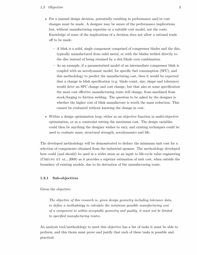
• For a manual design decision, potentially resulting in performance and/or costchanges must be made. A designer may be aware of the performance implicationsbut, without manufacturing expertise or a suitable cost model, not the costs.Knowledge of some of the implications of a decision does not allow a rational tradeoff to be made.
– A blisk is a solid, single component comprised of compressor blades and the disc,typically manufactured from solid metal, or with the blades welded directly tothe disc instead of being retained by a slot/blade root combination.
– As an example, if a parameterised model of an intermediate compressor blisk iscoupled with an aerodynamic model, for specific fuel consumption (SFC), andthis methodology to predict the manufacturing cost, then it would be expectedthat a change in blisk specification (e.g. blade count, size, shape and tolerance)would drive an SFC change and cost change, but that also at some specificationthe most cost effective manufacturing route will change, from machined fromstock/forging to friction welding. The question to be asked by the designer iswhether the higher cost of blisk manufacture is worth the mass reduction. Thiscannot be evaluated without knowing the change in cost.
• Within a design optimisation loop, either as an objective function in multi-objectiveoptimisation, or as a constraint setting the maximum cost. The design variablescould then be anything the designer wishes to vary, and existing techniques could beused to evaluate mass, structural strength, aerodynamics and life.
The developed methodology will be demonstrated to deduce the minimum unit cost for aselection of components obtained from the industrial sponsor. The methodology developedhere could (and should) be used in a wider sense as an input to life-cycle value engineering(Cheung et al., 2008) as it provides a superior estimation of unit cost, when outside theboundary of existing models, due to its derivation of the manufacturing route.
1.3.1 Sub-objectives
Given the objective:
The objective of this research is, given design geometry including tolerance data,to define a methodology to calculate the minimum possible manufacturing costof a component to within acceptable geometry and quality, it must not be limitedto specified manufacturing routes.
An analysis tool/methodology to meet this objective has a list of tasks it must be able toperform, and this thesis must prove and justify that each of these tasks is possible andpractical:

4 1 INTRODUCTION
Task 1 To deduce the shape created using additive or forming processes, and the costthereof of these processes.
Task 2 To determine what possible manufacturing processes can be used to make theremaining features (i.e. any not already created by the additive or forming process).
Task 3 To derive which of the possible manufacturing processes should be used to makethe remaining features.
Task 4 To deduce the optimal order in which these processes should be conducted.
Task 5 To make any remaining decisions such as tooling used, access direction.
1.4 Vision
Activity Based Costing (Qian/Ben-Arieh, 2008) combined with process optimisation isan incomplete field of study, and this is the area this research aims to improve. It goesbeyond the assumption that manufacturing routes are fixed (or manually constructed), toallow the manufacturing route to change in response to design geometry and tolerancedata. Furthermore, by taking into account compound scrap rates, the ideal manufacturingprocess will depend on the cost incurred up to that point (as proved in Section 5.4).
To demonstrate the need to go beyond the assumption of fixed manufacturing routes forsimilar components, a typical industrial example will be illustrated. We have twocomponents with the same purpose a and b, of a similar geometric design, but differingscales and manufactured years apart. It could be that the least costly manufacturing routefor both components is identical in content, although likely to be differing in operationtime. If we denote the least costly manufacturing route for component a as o, and the leastcostly route for b by p. Then p will be identical (in content) to o if:
• p was optimal at the time of its derivation, (i.e. before commencement of productionfor a).
• The two components are sufficiently similar in terms of G&T (Geometric andTolerance) data.
• o does not contain any manufacturing processes which were unavailable when p wasderived.
If b is sufficiently different from a, manufacturing advances have been made which shouldbe used in production of this component, or if p was suboptimal, then all newmanufacturing routes (or at least all those which might be cost effective) should beexplored. This can be done manually or computationally, using manufacturing knowledgeand rules. Thus this research aims to construct and demonstrate a systematic andautomated framework, which uses formally structured manufacturing knowledge.
1.5 Overall Architecture 5
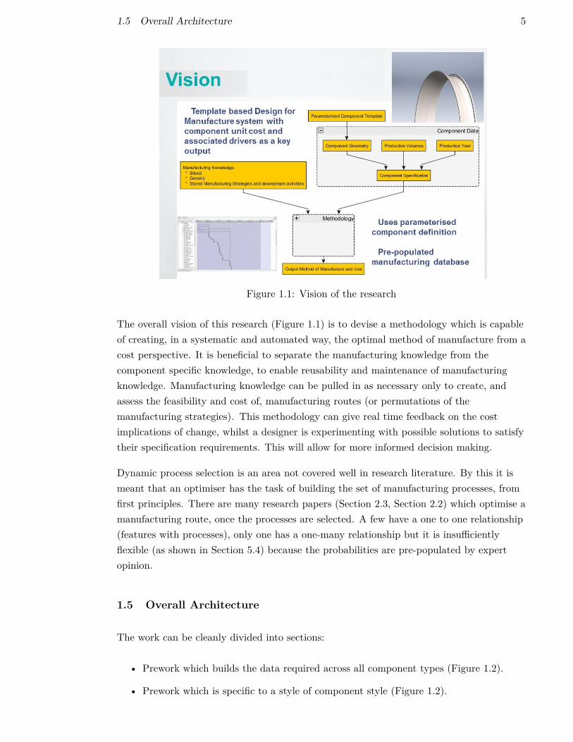
Figure 1.1: Vision of the research
The overall vision of this research (Figure 1.1) is to devise a methodology which is capableof creating, in a systematic and automated way, the optimal method of manufacture from acost perspective. It is beneficial to separate the manufacturing knowledge from thecomponent specific knowledge, to enable reusability and maintenance of manufacturingknowledge. Manufacturing knowledge can be pulled in as necessary only to create, andassess the feasibility and cost of, manufacturing routes (or permutations of themanufacturing strategies). This methodology can give real time feedback on the costimplications of change, whilst a designer is experimenting with possible solutions to satisfytheir specification requirements. This will allow for more informed decision making.
Dynamic process selection is an area not covered well in research literature. By this it ismeant that an optimiser has the task of building the set of manufacturing processes, fromfirst principles. There are many research papers (Section 2.3, Section 2.2) which optimise amanufacturing route, once the processes are selected. A few have a one to one relationship(features with processes), only one has a one-many relationship but it is insufficientlyflexible (as shown in Section 5.4) because the probabilities are pre-populated by expertopinion.
1.5 Overall Architecture
The work can be cleanly divided into sections:
• Prework which builds the data required across all component types (Figure 1.2).
• Prework which is specific to a style of component style (Figure 1.2).

6 1 INTRODUCTION
• Current design work on a specific instance of that component (Figure 1.3).
As shown in Figure 1.2:
• Design features require a mapping to one or more usable elemental features.
• Elemental features require one or more associated manufacturing features to beusable.
• Manufacturing processes require machines which can create them.
In order to create a component template, comprised of an NX model and ComponentIntegration Spreadsheet (CIS) (Section 1.6.3), it is necessary for design features to exist tocover all geometry.
It should be noted that in section 1.7.2, it is shown that Rolls-Royce is planning tointroduce a design by feature system. This, and its benefits in so far as this research isconcerned, will be explained in Section 1.7.2.
This component template can then be used to design a component of that type for aspecific application, its applicability will depend on the quality and flexibility of theparameterisation.
The component template can then be used (as in Figure 1.3) as the input to the designprocess for a specific application. After changing the geometry and/or tolerance valueswithin the bounds of the parameterisation, the methodology can be run to deduce theoptimal method of manufacture, and associated cost. This method of manufacture can bestored to enable very rapid re-analysis of cost (i.e. assuming a fixed method ofmanufacture). Of course the penalty of this is that this method of manufacture may nolonger be optimal. It cannot be known whether a point has been reached where themethod of manufacture should be changed, without rerunning the optimisation. A moredetailed diagram of the interactions between FoSCo and MCSOT is shown in Section 1.6.

1.5 Overall Architecture 7
Figure 1.2: Overall architecture - Prework

8 1 INTRODUCTION
Figure 1.3: Overall architecture - Current Design work
1.6 Methodology structure and interfaces 9
1.6 Methodology structure and interfaces
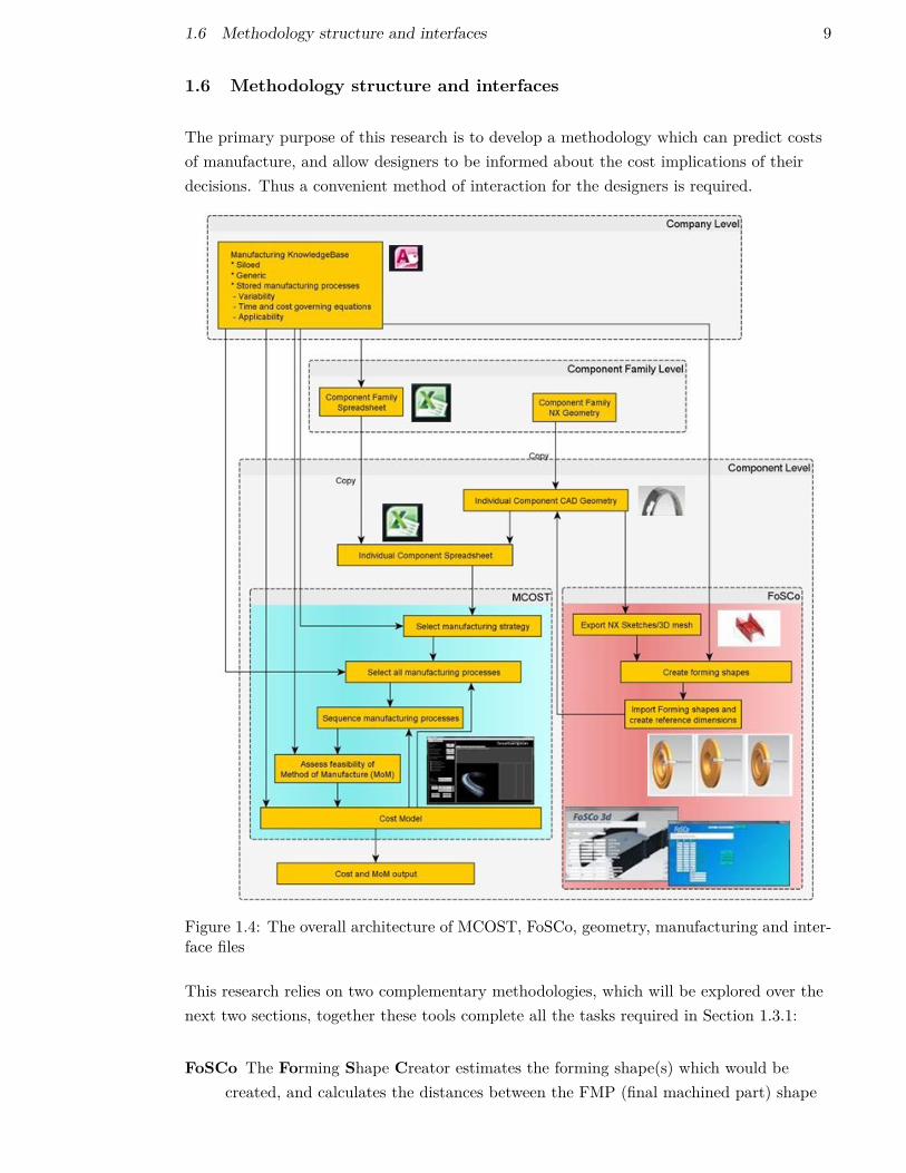
The primary purpose of this research is to develop a methodology which can predict costsof manufacture, and allow designers to be informed about the cost implications of theirdecisions. Thus a convenient method of interaction for the designers is required.
Figure 1.4: The overall architecture of MCOST, FoSCo, geometry, manufacturing and inter-face files
This research relies on two complementary methodologies, which will be explored over thenext two sections, together these tools complete all the tasks required in Section 1.3.1:
FoSCo The Forming Shape Creator estimates the forming shape(s) which would becreated, and calculates the distances between the FMP (final machined part) shape

10 1 INTRODUCTION
and the forming shape for later use by MCOST.Satisfies:
Task 1a To deduce the shape created using forming processes.
MCOST The Manufacturing Choice Optimisation and Sequencing Tool is the centralpiece of software, choosing how to manufacture the component, but relying oncomponent specifications, manufacturing knowledge and FoSCo.Satisfies:
Task 1b Calculate the cost thereof of these (forming) processes.
Task 2 To determine which possible manufacturing processes can be used to makethe remaining features (i.e. any not already created by the additive or formingprocess).
Task 3 To derive which of the possible manufacturing processes should be used tomake the remaining features.
Task 4 To deduce the optimal order in which these processes should be conducted.
Task 5 To make any remaining decisions such as tooling used, access direction, etc.
It was decided that the best method of interaction was an interface to Siemens NX, as thisis the industrial sponsor’s CAD geometry creation tool. As shown in Figure 1.4, MCOSTcan be launched from within NX when a cost analysis is desired. FoSCo must also be run(prior to MCOST) whenever the geometry is changed, if the change may result in a changein precursor shape.
It would be possible to code both FoSCo and (with more difficulty) MCOST to run directlyin NX Open (the NX Application Programming Interface), but from a research point ofview was deemed unnecessary given that it is arbitrary exactly where the component datais stored. Hence pragmatism has been used to determine the location of storage of relevantdata, and this research has elected to create a C# interface through excel and a csv file,rather than attempting to read directly from inside NX.
A fully automated method able to run multiple full optimisations, and store the results,was also coded, requiring simply a file detailing the required parameters for eachoptimisation. This allows multiple components to be optimised overnight (for example) oron a high performance cluster.
1.6.1 Software
The software used in this research is:
Siemens NX 8 Used for CAD modelling, this is simply because it is the industrialsponsor’s corporate tool, and thus they have relevant experience and models which

1.6 Methodology structure and interfaces 11
can potentially be reused. NX 8 was the version the University of Southampton hadat the time of this research.
C# General purpose programming language used for the majority of the analysis, C# isused due to its built-in GUI construction capability, speed advantage over MATLAB,and the ease with which customised data structures can be constructed.
Microsoft Excel Used mainly for data transfer and storage of component data. Usedbecause of the ease of interface with C#.
Microsoft Access Used as a prototyping tool to construct and edit the database whichstores manufacturing knowledge.
MatLab Used as a prototyping language for FoSCo due to its inbuilt graph plottingcapability. Used due to familiarity.
1.6.2 Created Tools
There have been multiple tools created during the course of this research, to prove thevalue of the developed methodology, these are outlined below:
FoSCo 2d The Forming Shape Creator takes a 2d sketch, estimates the forming shape(s)which would be created and calculates the distances between the FMP (finalmachined part) shape and the forming shape for later use by MCOST.
FoSCo 3d The Forming Shape Creator takes a 3d model, estimates the forming shape(s)which would be created and calculates the distances between the FMP (finalmachined part) shape and the forming shape for later use by MCOST.
2d/3d NX I/O 2d and 3d codes for NX interface to allow export to and import fromFoSCo and MCOST.
MCOST The Manufacturing Choice Optimisation and Sequencing Tool is the centralpiece of software, it creates a cost optimal manufacturing process by creating andsequencing the process, then choosing the machine and TAD for each operation.
Component Interface Spreasheet This is a spreadsheet which provides an interfacebetween the CAD geometry and MCOST (Section 1.6.3, Section 7.3).
1.6.3 The component model and spreadsheet
In Section 7.3 sections of the Component Interface Spreadsheet (CIS) are shown. Theseshow the method of linkage between the CAD geometry package (NX), and therepresentation of design features stored in the CIS. However in summary the essence is to

12 1 INTRODUCTION
name the dimensions in NX, export them as a .txt file, and pull them into the CIS using aVBA macro. They can then be referred to by name in the CIS.
MCOST will then read the design features in the CIS line by line and convert them intoelemental features, this is explained in Section 5.7.3.
A new component template will sometimes be required, because the current template forthis type of component does not have the correct design features, for example, or becausethere is no existing template for this type of component.
The method of creation is to concurrently construct a CAD model for the component andthe CIS, the CIS will contain (design) features, as will the CAD model. Dimensions in theCAD model must be named, and the CIS must refer to the appropriate name. Each row inthe design features sheet in the CIS (Section 7.3) represents a single design feature, thereare various geometrical and tolerance parameters which must be defined for the designfeature, dependant on the design feature definition in the knowledgebase (Section 1.6).

1.7 Industrial sponsor context 13
1.7 Industrial sponsor context
1.7.1 The Front Bearing Housing (FBH)
The author’s research was sponsored by Rolls-Royce and therefore the primary test casesused (Section 1.8) and the manufacturing processes incorporated in the knowledgebasereflect the preferences of them.
Test case one and two were both drawn from the front bearing housing assembly. Thisassembly includes both aerodynamic and structural components, and as such renders it asuitable assembly from which to draw test cases. The FBH is located directly behind thelow pressure compressor (Figure 1.5), and removes most of the swirl from core air inaddition to locating the front bearings, for the low pressure and intermediate pressuresystem shafts. CAD images of the assembly are shown in Figure 1.6, all of these fourdiagrams were obtained from the industrial sponsor. In addition as a validation exercise ablisk is used to prove the applicability of the forming shape creator (Section 4).
Figure 1.5: The location of the FBH in a typical engine (Rolls-Royce, 2013)
1.7.2 Feature Classification and standard features
The following figures and description are intended to show the possibility of automaticallybuilding cost models, during the definition of components within the CAD geometry. Thiscould wholly or partially remove the need to use feature recognition prior to processplanning, and would remove some of the overhead shown in Section 1.5, specifically the CISpart of the component specific prework.
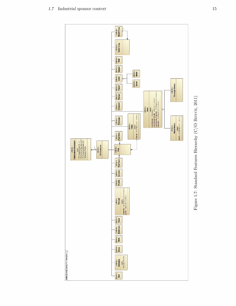
Rolls-Royce intend to design using standard features, by which they mean parameterisedCAD definitions of commonly used features, which can be superimposed on appropriatesurfaces/edges etc. of a CAD model. The hierarchy of these features is shown in Figure1.7. However, as can be seen some of the features are both design and manufacturing, someare simple, and some are compound features. This definition is thus incomplete and

14 1 INTRODUCTION
Figure 1.6: A front (Trent 1000) and rear (Trent 800) view of the Trent FBH (C/O Johnson,2012)
insufficiently formal, however, it is a starting point for a feature based design method suchas outlined in Section 2.1.2.
If completed and exclusively used, it could allow the automated building of cost models,including as an input to MCOST (Section 5). That is to say that the incorporation of adesign feature into a CAD model, could also update the CIS to include a new line for thedesign feature, and automatically link up the feature dimensions to named NX dimensions.
Rolls-Royce have been working on identifying a hierarchical model of feature classificationfor the various components of the FBH assembly as shown in Figure 1.8.
Following this feature classification Rolls-Royce has begun to identify the design andmanufacturing constraints in documents. As shown in Figures 1.9; 1.10.
1.7 Industrial sponsor context 15
Figu
re1.7:
Stan
dard
Features
Hierarchy
(C/O
Boy
ce,2
011)

16 1 INTRODUCTION
Figure1.8:
FBH
FeatureClassification
(C/O
Johnson,2011b)

1.7 Industrial sponsor context 17
Figure 1.9: Airfoil De-icing Holes Model and Drawings (C/O Johnson, 2011a)
Figure 1.10: Airfoil De-icing Holes Constraints (C/O Johnson, 2011a)
18 1 INTRODUCTION
1.7.3 Model Construction Data
It is assumed that all industrial companies attempting to predict and control costs willhave, at the very least, estimates of their future production volumes. In addition, it isassumed that they will have, or be able to construct, 3d geometry models usingparameterised design features.
For this research, the CAD package in which the components will be constructed will beNX81, simply because the expertise to extract data exists within the industrial sponsor.
The cost of production of a component can be divided into two categories:
Bought in cost This is the cost that a company pays to obtain raw materials or partfinished components.
Part finished components are, in extremis, only composed of raw material andmanufacturing costs.
Manufacturing cost This is the cost of the manufacturing operations necessary totransform the inputs of raw materials, or partly machined components into the FPG(Finished Part Geometry). These costs contain amortisation of indirect costs, as partof the accounting process.
This research will thus consider only raw material and a detailed breakdown ofmanufacturing costs, although clearly for bought in parts a profit margin will be implicitwithin all cost rates. Material cost estimates will be obtained directly from the industrialsponsor’s cost modelling department. In other words, this research will ignore thedistinction between the company’s internal and external supply chain, thus concentratingonly on the production cost. Commercial and political considerations will be ignored.
1.7.4 Manufacturing knowledge
Standard material removal processes have standard speeds predefined according to the typeof operation and the material number (a machinability index). An example of these tablesfor drilling is shown in Table 1.1. In addition, there exists similar data for other machiningoperations such as turning and milling, which can be inverted to give MRRs (MaterialRemoval Rates) for various chip forming manufacturing processes. This data is used inRolls-Royce cost models, and an extract is shown in Figure 1.11. These data will be usedon the cost model integrated within the methodology developed by this research.
1NX8 was the latest version the University of Southampton had available at the time.

1.7 Industrial sponsor context 19
DRILLING
SPEE
D(m
/min)
REA
MIN
GSP
EED
(m/m
in)
TAPP
ING
SPEE
D(m
/min)
Table
HighSp
eedSteel
Table
Carbide
Table
HighSp
eedSteel
Table
Carbide
Table
Speed
160
.85
112
1.70
122
.85
145
.70
117
.10
257
.85
211
5.78
222
.85
245
.70
212
.80
353
.45
310
6.90
322
.85
345
.70
312
.80
425
.95
451
.90
410
.65
421
.30
48.55
522
.95
545
.90
510
.65
521
.30
56.40
618
.35
636
.70
66.85
613
.70
65.35
718
.35
736
.70
76.85
713
.70
75.35
815
.15
830
.30
86.85
813
.70
85.35
913
.75
927
.50
96.10
912
.20
94.15
1013
.75
1027
.50
106.10
1012
.20
103.85
1112
.15
1124
.30
116.10
1112
.20
113.85
1212
.15
1224
.30
126.10
1212
.20
123.65
1310
.55
1321
.10
135.15
1310
.30
133.45
149.15
1418
.30
145.15
1410
.30
143.45
159.15
1518
.30
155.00
1510
.00
153.00
166.20
1612
.40
165.00
1610
.00
162.80
176.20
1712
.40
175.00
1710
.00
172.55
187.60
1815
.20
183.65
187.30
182.50
Table1.1:
Drillin
gspeedag
ainstman
ufacturabilityinde
xforseveraltyp
esof
drillingop
eration(C
/OW
isea
ll,2
010)

20 1 INTRODUCTION
Figure1.11:Anextractoflookup
tablecontainingprocessratesforsom
eofRolls-R
oyce’scommonly
usedmanufacturing
technologies(C/O
Reuss,
2010)

1.7 Industrial sponsor context 21
1.7.5 Verification/Validation Data
To verify convergence of the algorithm test case zero (Section 1.8) will be used, this is asimplified version of test case one, contrived to test the optimisation algorithm. To showconvergence toward the global optimum for other test cases, convergence graphs will beshown.
To validate the methods of manufacture output by MCOST, SAP ERP data will be used.This gives manufacturing routes, times and the cost, for each manufacturing operation inthe industrial sponsor’s internal supply chain.
The standard location for storage of Method(s) of Manufacture (MoM) in Rolls-Royce,once production has begun, is SAP ERP software (usually referred to as SAP). An exampleof an exported MoM from SAP (in CK-86 format) is shown in Figure 1.12. These datawere automatically extracted to produce manufacturing process plans of currentcomponents, and can be used for the validation of test case one. Cost data for test case twowas also used.

22 1 INTRODUCTION
Figure1.12:
Anexam
pleofa
CK-86
SAP
dataexport
with
numericallevels
C/O
Johnson(2010)

1.8 Test Cases 23
1.8 Test Cases
In order to demonstrate the applicability of the methodology whilst satisfying the customerdemands, multiple test cases will be used.
Test Case Zero One TwoComponent Simplified rear Rear outer Engine Section
outer casing casing Stator (ESS)Forming Method 1 Roll Forging Roll Forging ForgingForming Method 2 Centrifugal Casting Centrifugal Casting CastingForming Method 4 Machined from tube Machined from tube Machined from billet
Table 1.2: Test cases to be analysed
Three test cases are to be used, with multiple manufacturing strategies for each (Table1.2). Test cases zero, one and two are shown in Table 1.3. Test case zero is intended toshow that the methodology can find the global optimum, since it has been contrived to givea known optimum (for the created manufacturing knowledge database). Test cases one andtwo are intended to show accurate costs on different types of component, and are actualRolls-Royce components (though with non cost effecting features such as minor filletsremoved). Test cases zero and one are mainly axisymmetric, and the manufacturing willthus tend towards technologies such as ring roll forging, centrifugal casting, and turningtype operations. Test case two has no axisymmetry, and will thus rely more on die forging,milling, and other similar technologies not dependant on continuous rotation of thecomponent.
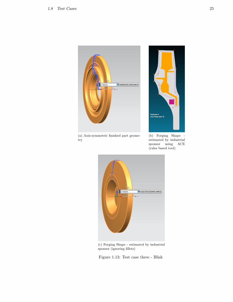
In addition to these test cases which were used for both MCOST and FoSCo, an additionaltest case (Figure 1.13) was incorporated purely for the testing of FoSCo. As it is an IPsensitive component Rolls-Royce did not want its manufacturing process included withinthis thesis, but an approximation of the outline geometry was acceptable. Figure 1.13shows the finished part geometry and forging shapes, as estimated by the IndustrialSponsor.
Because this research does not include feature recognition, but instead uses a mappingfrom design to elemental features, a design feature list is also needed for each test case.This is shown in Table 1.3. Note that because the methodology will deduce the optimalmachining order, the order in which the features are defined has no effect.

24 1 INTRODUCTION
Testcase
zeroTest
caseone
Test
casetw
oD
esignfeature
name
Design
featuretype
Design
featurenam
eD
esignfeature
typeD
esignfeature
name
Design
featuretype
Rear
Outer
Casing
Condition
ofSupply-C
ylindricalRear
Outer
Casing
Condition
ofSupply-C
ylindricalEngine
SectionStator
Condition
ofSupply-B
illetOuter
SlotsSlot
Group
SetRotated
PadsPad
Lower
VaneSurface
Concave
Slot
InnerSlots
SlotGroup
SetRotated
Weight
ReliefSlots
SlotGroup
SetUpper
VaneSurface
Convex
Slot
FlangeFlange
Bolt
andDow
elHoles
Through
Holes
Counterbored
SlotsOuter
SlotGroup
VariableStator
VaneActuator
(VSVA
)Holes
Through
Holes
Double
Counterbored
SlotsInner
SlotGroup
VSVA
Bosses
Bushes
SlotsTop
SlotGroup
Mounting
FlangeFlange
SlotsBottom
SlotGroup
SlotsInner
Multi-stage
Groove
ServicesAccess
SlotSlots
Outer
Multi-stage
Groove
Mounting
Bracket
Bracket
FacesInner
FacesFaces
Outer
Faces
Table1.3:
Testcases:
Design
featurelist
1.8 Test Cases 25
(a) Axis-symmetric finished part geome-try
(b) Forging Shape -estimated by industrialsponsor using ACE(rules based tool)
(c) Forging Shape - estimated by industrialsponsor (ignoring fillets)
Figure 1.13: Test case three - Blisk

26 1 INTRODUCTION
1.8.1 Minor Test Cases
In addition to the three primary test cases, 20 other cases were tested, to ensure that themethodology was able to cope with them without modification. These were provided bythe industrial sponsor, and were the same as used by the sponsor to investigate the qualityof the commercial tool aPriori, evaluated in Section 3.2.
The only modification required for accurate results, was enabling the methodology to takeaccount of batch production2. Enabling the machine setup time to be amortised over allcomponents in the batch is necessary to ensure accurate costing estimation.
The minor test cases have been split according to whether they contain mainlyaxis-symmetric features or not. This will determine how the formed shape is modelled byFoSCo (Forming Shape Creator), as there are two different versions. There is nodistinction in MCOST. In addition the user must choose a shape to create as the initialshape, as different manufacturing processes and cost rules apply to rectangular billets, barsand tubes, be they forged, cast or supplied from supplier stock (the last choice can bemade by MCOST).
The test cases are shown in Table 1.4 Table 1.5:
2This is part of future work.

1.8 Test Cases 27
Table 1.4: The 10 minor mainly axisymmetric test cases
Table 1.5: The 10 minor non-axisymmetric test cases

28 1 INTRODUCTION
1.9 Papers and patents
A patent application related to FoSCo (see chapter 4) has been filed, in 2015 (in the UK),on the industrial sponsor’s instructions.
This was withdrawn and an application was made for a US and EU patent by theindustrial sponsor. The intention is to use this methodology in preliminary design.
EU patent number 16180366.3 - 1954
US patent submission reference 5895 LMT
1.10 Thesis synopsis
Section 2: Literature Survey Section 2 details the academic research currentlyavailable, mainly exploring process planning, cost modelling and precursor shapeprediction. It also explores the complementary technology of feature recognition, thedesign process, and manufacturing processes.
Section 3: Commercial Costing Systems Section 3 details and critiques commercialcosting systems currently available. Commercial systems invariably have some formof feature recognition, presumably because it is much easier to sell to customers aproduct which does not require any significant change in the design method. Howeverat present they are limited in not considering the manufacturing sequence, thusreducing their effectiveness when the manufacturing process has a non trivial chanceof causing rework, scrap or concessions due to the tolerances being close to or tighterthan the variability of the manufacturing process.
Section 4: FoSCo (Forming Shape Creator) Section 4 details the methodology usedto predict the forming shape, i.e. the shape generated by the forming or additiveprocess. It is subdivided into the axis-symmetric version and the 3d version, althoughas will be seen the axis-symmetric operates in the same way where z is always zero.This methodology is necessary for the optimisation below to operate, as without anaccurate estimate of material removal volumes, it is impossible to accurately estimateoperation times. Having explained the methodology it continues to present results,and opportunities for further work.
Section 5: MCOST (Manufacturing Choice Optimisation and Sequencing Tool)Section 5 details the methodology used to construct and optimise the manufacturingroute, including the operation of the objective function (cost model). It includes adescription of the data storage necessary for the methodology to operate.Optimisation of the process route takes account of the choice of manufacturingprocesses, sequencing, tool access direction and the optimiser attempts to minimise

1.10 Thesis synopsis 29
unit cost. As above it presents results and further research and improvementopportunities.
Section 6: Conclusions Section 6 details the conclusions arrived at during this research,and some suggestions for the future direction (of FoSCo, MCOST, and methods toreduce the overhead of using these methods) which could be taken.
Section 7: Appendix MCOST and FoSCo additional information Section 7 hasadditional digrams and description related to the operation of MCOST and FoSCo, itis referred to from Sections 4 and 5.
Section 8: Appendix FoSCo patent submission Section 8 contains the full patentapplication for FoSCo.

30 1 INTRODUCTION

31
2 Literature Survey
A requirement has been established to embed cost knowledge into the design engineeringand process planning team. It can be seen, that cost modelling once the production processis decided, is a relatively well developed area. The main area of improvement, is thereforethought to be analysis and optimisation of possible manufacturing routes, from designgeometry, whilst cost modelling each iteration. This section of the thesis details theacademic literature related to this subject. The logical extension of this is then to combinewith life cycle modelling and conduct value analysis (discussed in Section 2.1.6), combinewith factory modelling to see the dynamic effects on the supply chain, or both. Howeverboth of these will be defined as out of scope, with the research limited to attempting toautomatically deduce the minimal cost method of manufacture, assuming a supply chainwith unlimited capacity and load independent costs.
To begin with, the process by which components are designed and prepared formanufacture, from a top-level perspective, will be reviewed. This section will also reviewalternative methods of design, and geometry creation. A review of the methods used forprocess planning, from the point of view of supply chain management, will be conducted.The section will continue on to high fidelity process planning methods, thus exploring thecomputer aided process planning (CAPP) area of the literature. This continues intomethods of representing and exploring the process planning search space, and analysis willbe conducted on the methods of linking CAPP to the geometry creation stage of design.
Following on from this, the author will explore the Computer Aided Manufacture (CAM)literature and the manufacturing methods which can be used, each manufacturing methodhas limitations on its use, and properties associated with it, which any process plannermust know, if they wish to make use of that particular manufacturing process.
It is then necessary to explore methods of cost modelling which can be used, where theyare useful and what information they require to produce accurate data. Particularattention is focussed on generative cost modelling, because of its ability to link directly intothe outputs of CAPP.
Finally, although out of scope, it is noted that there could be linkages between simulation,cost modelling and process planning. This would give the potential for a morecomprehensive tool, to further improve the design of components. This is because the costof machinery is in part dependant on the machine loading.
2.1 The Design Process
It is widely held to be the case, that design changes made later in the design process, aremore costly in both time and money, as stated by Xu et al. (2006). Later in design more
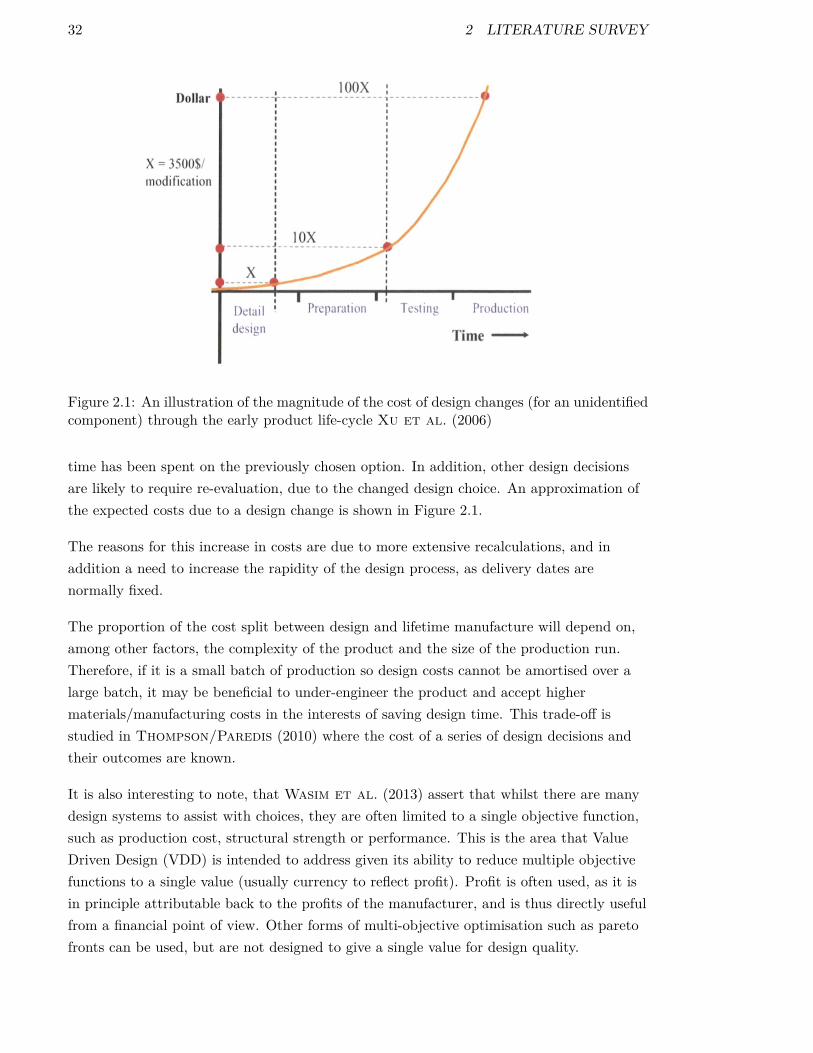
32 2 LITERATURE SURVEY
Figure 2.1: An illustration of the magnitude of the cost of design changes (for an unidentifiedcomponent) through the early product life-cycle Xu et al. (2006)
time has been spent on the previously chosen option. In addition, other design decisionsare likely to require re-evaluation, due to the changed design choice. An approximation ofthe expected costs due to a design change is shown in Figure 2.1.
The reasons for this increase in costs are due to more extensive recalculations, and inaddition a need to increase the rapidity of the design process, as delivery dates arenormally fixed.
The proportion of the cost split between design and lifetime manufacture will depend on,among other factors, the complexity of the product and the size of the production run.Therefore, if it is a small batch of production so design costs cannot be amortised over alarge batch, it may be beneficial to under-engineer the product and accept highermaterials/manufacturing costs in the interests of saving design time. This trade-off isstudied in Thompson/Paredis (2010) where the cost of a series of design decisions andtheir outcomes are known.
It is also interesting to note, that Wasim et al. (2013) assert that whilst there are manydesign systems to assist with choices, they are often limited to a single objective function,such as production cost, structural strength or performance. This is the area that ValueDriven Design (VDD) is intended to address given its ability to reduce multiple objectivefunctions to a single value (usually currency to reflect profit). Profit is often used, as it isin principle attributable back to the profits of the manufacturer, and is thus directly usefulfrom a financial point of view. Other forms of multi-objective optimisation such as paretofronts can be used, but are not designed to give a single value for design quality.

2.1 The Design Process 33
2.1.1 Concurrent vs Iterative Loop Engineering
Concurrent Engineering (CE) is a system of engineering, where engineering activities whichwere traditionally carried out in a sequential way are carried out simultaneously. Asexplained by Gao et al. (2008):
“CE is a philosophy that suggests the need to consider design issuessimultaneously where they were considered sequentially in the past”.
The main purpose of CE is the shortening of lead times, thus enabling the adoption oftechnology earlier than otherwise to gain competitive advantage. There are severalmethods to analyse the benefits (positive or negative) of concurrent engineering, some ofwhich are detailed by Gao et al. (2008), in addition to their suggestions on improvingthe design process. This analysis is beyond the scope of this work, but this section issimply an illustration of alternative design methods.
In contrast to concurrent engineering iterative loop engineering requires the conducting ofa series of tasks iteratively, and using the output of one task to guide another, for examplerepeating design and CAPP iteratively until a design which fulfils all design requirementsis created, then progressing to manufacturing.
A paper by Khoshnevis et al. (1994) presents a Real Time Computer Aided ProcessPlanning (RTCAPP) system. The system indicates to the designer the cost implications oftheir decision in real time, as they are designing a part, by producing a process plan usingdynamic programming and a knowledge based process planner. This paper is significant, inthat it is the only paper found, which states the intention to be used by designers toconsider the implications of their design decisions, but also uses generative processmodelling. It reuses as much of the existing process plan as possible, thus reducingoptimisation time, although the benefit of this will vary according to the magnitude andtype of the changes. The system designed by Khoshnevis et al. (1994) can be used forprismatic parts, and it is assumed that the cost rates for machinery are pre-defined sinceno mention is made in the paper to the contrary.
Tammineni et al. (2009) use a form of concurrent engineering in their knowledge basedsystem (Figure 2.2). Input to the distributed knowledge base, is performed by experts inthe relevant area: designers, cost modellers and manufacturing engineers, who interactthrough the knowledge base library and manufacturing databases. This type of knowledgestorage is particularly of interest to large organisations, as they have experts in the variousfields. The relevant expert can therefore be given permission to alter only the section of theknowledgebase relevant to their expertise.
Set-Based Concurrent Engineering is a concept developed by Toyota and explained byMorgan/Liker (c2006.). One of the concepts they analyse is the possibility of multiple

34 2 LITERATURE SURVEY
Figure 2.2: A knowledge-based system for cost modeling Tammineni et al. (2009)
streams of engineering working continuously, which together can deliver the necessary goal.The end result of the design which is produced is an area of the design space which allnecessary parties agree they can achieve. The main advantages of this process over typicaldesign iterations in series are:
1. A reduction in lead time since component design and manufacturing design areconducted in parallel rather than in a serial loop format typical of most designsystems.
2. A right first time approach reducing wasted resources due to uncertainty ofpracticalities.
It should be noted that set-based concurrent engineering as described by Morgan/Liker(c2006.) (Figure 2.3) is different to design loops (the iterative model) although they areoften taken to be synonymous. The iterative approach sequentially passes informationbetween different designers where each team will accept or reject the modifications to thedesign requested by the previous teams until a time limit is reached (Figure 2.3). It shouldbe noted that this is illustrative, and not an exhaustive set of the design activities. Inset-based concurrent engineering different teams will generate and analyse many designs fortheir particular function (for example body, chassis and suspension) simultaneously; systemengineers will then decide which set of designs will be used for the product, which must belocated in the region of the design space which all relevant departments agree is feasible.To illustrate this there will be aesthetically pleasing and aerodynamically efficient bodies toa car which are perfectly feasible to make, but a practical chassis cannot be designed forthem at an acceptable cost, designs of this type would be rejected by the systems

2.1 The Design Process 35
Figure 2.3: The iterative and concurrent design process models for (a subset of activities in)a generic aerospace design processes
engineers. If no set of feasible solutions can be found, the closest solutions are returned tothe design teams to narrow in on a solution (thus resulting in some iteration). Thisapproach is thought to reduce lead time, prevent the inefficiencies of loops and deliver anoptimal solution rather than just a possible solution which is optimal only to the last teamto alter the design before the cut-off time is reached.
It can be inferred that although concurrent engineering minimises lead time, it isinherently wasteful, as multiple designs which will not be taken forward are produced. Itcan, however, be argued, that it produces superior designs, as more are considered, andthus more flexibility is present. Typically iterative loop design only continues until aworkable design is reached, which may or may not be optimal.
In the author’s opinion, concurrent loop engineering is most useful for semi-independentsystems. The greater the inter-dependence between systems, the more design effort mustbe expended. Concurrent engineering by its nature requires either: pre-defined interfacesand specifications affecting other components, or, teams must anticipate other team’sdecisions and prepare for them in their design.
2.1.2 Potential Design Methods
The purpose of a design process is to produce a design which satisfies all designrequirements, including manufacturability at an acceptable cost. It must therefore becomposed of features which can be manufactured, and should best satisfy the cost-valuetrade-off. As stated by Grabowik et al. (2005) a typical design process involves a designphase followed by a process planning phase after the design is complete. However, theeffect of considering the manufacturing process after completing detailed design, is anincreased difficulty and cost of design changes if changes are required.
Manufacturability can either be checked separately or considered as a part of CAPP.

36 2 LITERATURE SURVEY
Manufacturability checking without CAPP however typically assumes a knownmanufacturing route, which this research goes beyond. Two possible automated methods ofchecking manufacturability are stated by Di Stefano et al. (2004) are shown as 1 and2(a) in the list, 2(a) and 3 are alternative options for the integration of CAD withmanufacturing optimisation:
1. Produce the design as a solid model and use automated feature recognition todecompose the design into manufacturable features.
2. Design by feature using features which have at least one potential manufacturingroute associated with them.
(a) Either the designer can explicitly select the manufacturing method using ahierarchy.
(b) Or the computer can choose a manufacturing method for each manufacturingfeature.
3. CAD is conducted using design features, which are then converted intomanufacturing features
(a) The designer specifies a feature, geometry, tolerances and surface finish and thecomputer will use manufacturing rules to determine the optimal way of doing it,or present a series of options.
(b) The designer specifies an intention and the computer will specify a feature,geometry, tolerances and surface finish and then use manufacturing rules todetermine the optimal way of doing it, or present a series of options(Brunetti/Golob (2000)). This is discussed in Section 2.1.5.
There are advantages and disadvantages associated with each of these possibilities whichare outlined in Table 2.1:
2.1.3 Features
The study of features is a wide ranging and extensive topic and necessary for both designfor manufacture systems, and some design systems as well.
There are several definitions to be discussed:
Design Features These are features utilised by designers to achieve certain aims, forexample:
• To provide structural rigidity

2.1 The Design Process 37
(1)Sk
etch
based(solid
mod
el)CAD
and
featurerecogn
ition
2(a:b)
Explicit
Man
ufacturin
gMetho
d3(a:b)
Com
puterSe
lectionof
Metho
d
Adv
antages
•Ex
trem
elyfle
xiblewhe
nconfi
gured
•Allo
wsde
signe
rcompletefreedo
m
•Relativelyeasy
toim
plem
ent
•2(b)
includ
esop
timisa
tion
•Com
puterSe
lectsman
ufacturin
gPr
ocess
•Kno
wledg
eof
metho
dselectioncan
beinpu
tby
anexpe
rt
•Doesno
trely
onthede
signe
rha
ving
specialistkn
owledg
e
•Can
give
results
quickly
•Increasedprod
uctiv
ityof
desig
ner
Limita
tions
•Po
ssible
issue
swith
ellip
tical,
complex
compo
nents
•Not
themetho
dof
desig
nRolls-
Royce
wish
topu
rsue
•W
hatto
dowhe
nmultip
lefeature
combina
tions
arepo
ssible
•Po
ssible
compu
tatio
nalissue
s(real
timefeed
back
tode
signe
rs)
•Fe
aturerecogn
ition
notfully
solved
•DesignTe
amselectsman
ufacturin
gmetho
d(the
ymay
notha
vethe
necessaryexpe
rtise
)
•New
mod
elsne
cessaryto
take
accoun
tof
new
man
ufacturin
gprocesses
•Onwha
tcrite
riado
esthecompu
ter
select
metho
d(cost/qu
ality
/lead
time)
•Com
plex
towrit
ethe
man
ufacturin
grules
•Fe
atureinteractions
•To
leranc
einteractions
•Highlevelo
foptim
isatio
nne
eded
Table2.1:
Adv
antagesan
dDisa
dvan
tageswith
featureba
sedde
signan
dfeaturerecogn
ition

38 2 LITERATURE SURVEY
• To provide aerodynamic/hydrodynamic surfaces to guide fluids orincrease/reduce pressure
• To alleviate stresses
• To locate other components
• To enhance ergonomics/aesthetics
Manufacturing Features These are features created by specific stages in themanufacturing process, they fall into multiple categories:
Intermediate Steps, Serving no fundamental purpose apart from the fact that theoperation stops there before another takes over. For example where a roughingoperation ceases and a finishing operation starts. That is to say they are aconsequence of the manufacturing rather than a driving factor.
Finished geometry features Features that are created by a single manufacturingoperation that exist on the finished part geometry.
Fixturing Features Features required for fixturing purposes, for clamping/locatingthe component on capital equipment.
Reference Features Features required for referencing other features duringproduction, for example a particular feature may have a tolerance definedagainst another feature which may/may not still exist when the part is finished.
The set of manufacturing features will of course determine the possibilities ofmanufacturing processes which can be used to make the component and also the potentialsequences which are feasible.
2.1.4 Feature Recognition
Feature Recognition in this context is the process of automated deduction ofmanufacturing features from the designer’s CAD geometry creation tool. However, it isworth noting that it can have several starting points:
1. In a feature based design environment translation from design features tomanufacturing features is required. Translators have been developed including toolssuch as ontologies, spreadsheets and the AP-224 translator used by Xu et al. (2005)to translate between design features and manufacturing features.
2. Where features are created through the use of sketches rather than built in featuresof the CAD package graphical identification of the component is required, which mayconvert the geometry directly to manufacturing features or may have design featuresas an intermediate step.

2.1 The Design Process 39
Figure 2.4: A diagram representing a feature recognition based design method
To convert design geometry into a component it is manufactured in general by a series ofoperations which create features using fundamentally different manufacturing methods.The reasons for these differences are partially due to the method of force application, forexample a hole will probably be drilled or punched whereas a groove with rotationalsymmetry will be turned and a groove without rotational symmetry will be milled. It isclear that milling will have a lower material removal rate than drilling (assuming aconstant size of tool) because the force exerted is a torque on the side of the tool ratherthan a compressive force. In turning however, the shape of the tool can allow shear loadingand thus turning is faster in general than milling for a given removal volume. The accessdirection relative to both the part and the surface on which it is being machined is also amajor contributing factor due to the loading on both the machine and the part.
The manufacturing features must be created from the difference between the finalmachined design geometry and the geometry created by the forming method ofmanufacture. There are several methods to do this: human conversion, Automated FeatureRecognition (AFR) or the designer specifying the manufacturing feature during design(explored in the next section). Humans are naturally good at this operation for simpleshapes as it can be done by intuition and experience, however, having people in the loopprohibits the vast number of evaluations necessary for optimisation and requires trainingand experience. According to Han et al. (2000) feature recognition takes CAD geometrywith modelling features and converts to manufacturing features as shown in Figure 2.4.The three main approaches to feature recognition according to Han et al. (2000); Babicet al. (2008) take the finished modelled geometry from a CAD program and involvedifferent techniques of extracting data from geometric models:

40 2 LITERATURE SURVEY
Figure 2.5: Volumetric Decomposition: Cell Decomposition Babic et al. (2008)
1. Volumetric decomposition
(a) Convex hull decomposition
(b) Cell decomposition
2. Graphical algorithms
3. Hint based geometric reasoning
The ways that these approaches work are shown below:
Volumetric Decomposition Works by applying volume identification algorithms tofinished component solid model data.
Cell decomposition Works by dividing the space into many small cubic volumes,calculating if material is present in the small volume and then recombiningempty volumes to create features, as in Figure 2.5. There are issues withcomplexity, particularly when the component involves curved surfaces as inDong/Vijayan (1997a).
Convex Hull decomposition Works in a similar way to cell decomposition butwith variable geometry polyhedral shapes instead of the cubic volumescharacteristic of cell decomposition as shown by Dong/Vijayan (1997b); Kim(1992).
The fundamental problem with both of these types of volumetric decomposition restsin their inability to work with non-polyhedral type shapes (in other words any shapewith finite curvature) unless a high density sample is generated, in which case vastdata manipulation and some degree of approximation is required. To rectify thisshortcoming Graphical Algorithms were developed.
Graphical Algorithms An early example of this approach was published byJoshi/Chang (1988), they define a face adjacency graph which maps the adjacentfaces to determine if they are concave or convex. From this graph feature subgraphscan be extracted and compared against a set of predefined feature graphs to identify

2.1 The Design Process 41
the feature. The algorithm recognises some feature interactions through splitting andre-joining graphs as necessary but there are still some issues; if a feature is notrecognised then the algorithm can return a not recognised message in preference toan incorrect match.
A more advanced algorithm allows a wider range of relationships between faces(Di Stefano et al., 2004). This predefined geometry can take forms including arcssuch as circular holes and slots with rounded ends. One of the methods reviewedworked by identifying faces and then testing all faces with all other faces to checkwhether the faces were:
1. Parallel
2. Perpendicular
3. Coaxial
4. Coincident
As shown in Figure 2.6, this approach identifies joins between two faces as secondaryfeatures and categorises them according to the angle between the faces. Once thefaces and their relationships are identified, additional data is attached to each node(representing each face). The additional data is:
Number of loops indicates the total number of loops of the face
Number of handles indicates the number equivalent handles of the face
Concavity indicates the concavity of the faces. A face of the model can be convexor non-convex. A face of the model is considered non-convex if one or both ofthe principal curvatures in at least a point of the face are negative. Otherwise itis considered convex.
Geometry indicates the geometry of the face, in compliance with the taxonomydepicted in Table 1 of Di Stefano et al. (2004).
Geometrical parameters indicate geometric characteristic of a particular shape(e.g. the radius and centre of a sphere, the axis the base point and the radius ofa cylinder), as stated in Table 1 of Di Stefano et al. (2004).
Face visibility indicates if a face is completely visible from, at least, one direction.A visible face has a nonempty visibility map. More details about accessibilityand visibility of faces are provided in Section 4 of Di Stefano et al. (2004).
Total visibility When all points on the face are visible along the same vectorNot visible If there are points on the face which are not visible
Face accessibility Indicates if a face is completely accessible from at least onedirection.
Once all of the faces have been identified there is more processing to identify whattype of surface the plane is according to categorisation, then further processing to
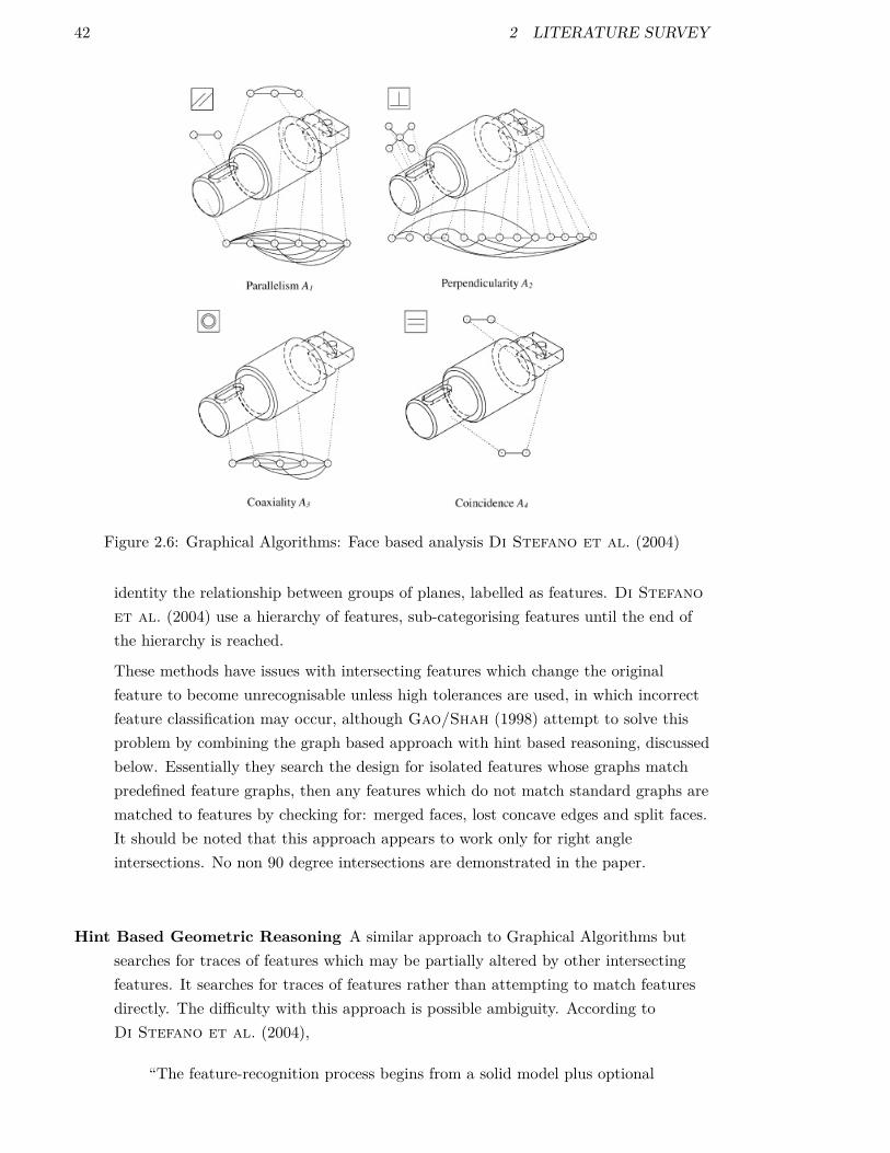
42 2 LITERATURE SURVEY
Figure 2.6: Graphical Algorithms: Face based analysis Di Stefano et al. (2004)
identity the relationship between groups of planes, labelled as features. Di Stefanoet al. (2004) use a hierarchy of features, sub-categorising features until the end ofthe hierarchy is reached.
These methods have issues with intersecting features which change the originalfeature to become unrecognisable unless high tolerances are used, in which incorrectfeature classification may occur, although Gao/Shah (1998) attempt to solve thisproblem by combining the graph based approach with hint based reasoning, discussedbelow. Essentially they search the design for isolated features whose graphs matchpredefined feature graphs, then any features which do not match standard graphs arematched to features by checking for: merged faces, lost concave edges and split faces.It should be noted that this approach appears to work only for right angleintersections. No non 90 degree intersections are demonstrated in the paper.
Hint Based Geometric Reasoning A similar approach to Graphical Algorithms butsearches for traces of features which may be partially altered by other intersectingfeatures. It searches for traces of features rather than attempting to match featuresdirectly. The difficulty with this approach is possible ambiguity. According toDi Stefano et al. (2004),
“The feature-recognition process begins from a solid model plus optional

2.1 The Design Process 43
information as tolerance, attributes and functional form features. Featureshints, which may result from particular combinations of part faces or bytolerance or attribute specification, are investigated and processed in orderto generate the largest possible feature volume consistent with the availabledata.”
We can see from authors such as Babic et al. (2008) that hint based reasoning isused to select the largest geometric feature which could be used to create anidentifiable trace in the design. Several techniques have been used to provide aninput to the algorithms including trimetric or orthographic drawings and the“viewer-centred approach” proposed by Sommerville et al. (2001) which takesseveral views of the component by taking an external point, drawing vectors out ofthe point and analysing where the vectors first intercept the component.
Similarly Vandenbrande/Requicha (1993) use an approach based on searching forpartial geometry on features to detect features which have faces or edges missing dueto other features. They restrict the possible features using criteria includingaccessibility, non-intrusion and presence. That is to say the feature candidate mustnot intrude upon the part, it must be fully accessible and it must leave a trace on thecomponent otherwise there is no functionality from it. They also consider the use ofmaterial removal volume intersections through optional and required portions:required portions are those where only one feature affects that volume; optionalportions are when more than one feature could remove the necessary volume.
Feature candidates are selected from pre-defined and hard-coded primitives (features)or composite features (sets of primitives). The system essentially generates featureswhich may lead to the hints which it has detected from the geometry and then teststo see if the feature is valid and expands the feature to ensure the largest possiblenon-intrusive feature is tested; then it validates the resulting geometry against thereal geometry, e.g. by checking that the required portions are indeed removed. Thisgenerate and test cycle continues, until the geometry which results from themachining is the same as the CAD geometry of the part.
An example feature recognition algorithm (Zhou et al. 2007)
A detailed algorithm for conversion of modelling features to manufacturing features ispresented by Zhou et al. (2007) (see Figure 2.7):
1. Get the modelling features (F0) one by one from the CAD model object using APIsprovided by the CAD platform.
2. Extract the geometry entities of F0, including its 2D sketch or profile (if it exists),and get the surface set of the created feature.

44 2 LITERATURE SURVEY
Figure 2.7: Feature recognition and feature tree reconstruction (Zhou et al., 2007)
(a) Identify surface adjacent relationships among the surface set by crossing theoutside normal vectors of every two adjacent surfaces and dotting with thedirectional vector of the common edge to get the angle (constraint) betweenadjacent surfaces. If the angle is less than 180, two surfaces are adjacent througha concave edge. Otherwise, two surfaces are adjacent through a convex edge. Inthe case of a freeform surface, the normal vector at the neighbourhood near thecommon edge can be used to determine the concave or convex attribute, and theneighbourhood can be obtained along two intersection curves that are createdby intersecting a plane normal to the common edge with two adjacent surfaces.
(b) Detect constraints between surfaces that do not join together directly by vectoroperation on outside normal vectors of such two surfaces; if their normal vectorsare opposite, it means there exists a parallel constraint between these twosurfaces.
(c) Analyse the adjacent character of the surface set, detect all subsets of surfacesthat are joined together, and determine available kinds of form features (FF)created by the F0 by comparing each subset of surfaces and the relatedconstraints with the predefined form feature templates. If more than one featureis created, record their twin relationship for application feature mapping.
(d) Calculate feature parameters and extract the form feature instances, includingcalculating the distance between two parallel surfaces, inheriting parametersfrom F0 and the parent feature to which the form feature is attached, andderiving the feasible tool access directions from the axis direction, modelling theoperation direction of F0, and/or outside normal directions of the corresponding
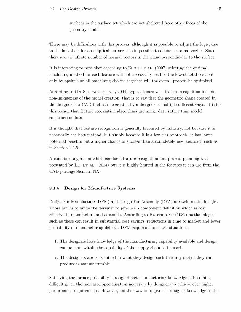
2.1 The Design Process 45
surfaces in the surface set which are not sheltered from other faces of thegeometry model.
There may be difficulties with this process, although it is possible to adjust the logic, dueto the fact that, for an elliptical surface it is impossible to define a normal vector. Sincethere are an infinite number of normal vectors in the plane perpendicular to the surface.
It is interesting to note that according to Zhou et al. (2007) selecting the optimalmachining method for each feature will not necessarily lead to the lowest total cost butonly by optimising all machining choices together will the overall process be optimised.
According to (Di Stefano et al., 2004) typical issues with feature recognition includenon-uniqueness of the model creation, that is to say that the geometric shape created bythe designer in a CAD tool can be created by a designer in multiple different ways. It is forthis reason that feature recognition algorithms use image data rather than modelconstruction data.
It is thought that feature recognition is generally favoured by industry, not because it isnecessarily the best method, but simply because it is a low risk approach. It has lowerpotential benefits but a higher chance of success than a completely new approach such asin Section 2.1.5.
A combined algorithm which conducts feature recognition and process planning waspresented by Liu et al. (2014) but it is highly limited in the features it can use from theCAD package Siemens NX.
2.1.5 Design for Manufacture Systems
Design For Manufacture (DFM) and Design For Assembly (DFA) are twin methodologieswhose aim is to guide the designer to produce a component definition which is costeffective to manufacture and assemble. According to Boothroyd (1982) methodologiessuch as these can result in substantial cost savings, reductions in time to market and lowerprobability of manufacturing defects. DFM requires one of two situations:
1. The designers have knowledge of the manufacturing capability available and designcomponents within the capability of the supply chain to be used.
2. The designers are constrained in what they design such that any design they canproduce is manufacturable.
Satisfying the former possibility through direct manufacturing knowledge is becomingdifficult given the increased specialisation necessary by designers to achieve ever higherperformance requirements. However, another way is to give the designer knowledge of the

46 2 LITERATURE SURVEY
cost implications of their designs without requiring them to acquire manufacturingexpertise, through the use of fully automated process planning and cost modelling system.This would enable the designer to test the cost implications of several possible designs tofulfil a design requirement without requiring manufacturing engineer analysis or for thedesigner to have expertise in manufacturing.
The latter can be too restrictive, prohibiting good but unusual solutions to issues such asweight reduction and raw material usage. Some methods of allowing restricted designs areelaborated on below.
Designing by Feature Library According to Xu et al. (2011) there are two ways ofdesigning by a feature library. The first step is to determine the input shape and material;which may be a bespoke shape or may be readily available industry standard stock. This islikely to depend on the purpose of the product, production size and the specifications ofthe finished part.
Destruction bymachining features Starts with the model of the raw stock from whicha part is to be machined. The design model is then generated by subtractingdepression features corresponding to the material to be removed by machiningoperations from the stock.
Synthesis by design features Synthesis by the design features method is built by bothadding and subtracting features.
According to Hoque/Szecsi (2008) designing from a feature library is alreadyimplemented within software such as Pro/Engineer. This is becoming normal practice inother CAD packages such as Solidworks and NX as well. Hoque/Szecsi (2008)supplemented this library with manufacturing rules which will produce error messages ifthere is an issue with manufacturing. However, the features demonstrated are relativelysimple, with limited interaction, such as single holes or slots. The features are arranged inhierarchies and the designer navigates down the hierarchy until they reach a final stage,and they supply the appropriate set of data, a flowchart of this method of design process isshown in Figure 2.8. In Hoque/Szecsi (2008) the designer is also required to select themethod of manufacture before choosing the precise feature. An example of a feature libraryand a parameterised drilled hole are shown in Figure 2.9.
Clearly this method relies upon some form of concurrent engineering type practice (Section2.1.1), since different engineers are required to write the rules for the requiredmanufacturing methods in a database or similar knowledge repository. A similar approachhas been taken by Hu et al. (2009) using DM (Design and Manufacture) features. Theyexplore the link between taking feature drawn CAD geometry and CAM whereasHoque/Szecsi (2008) restrict the scope to what is possible within manufacturing rules.
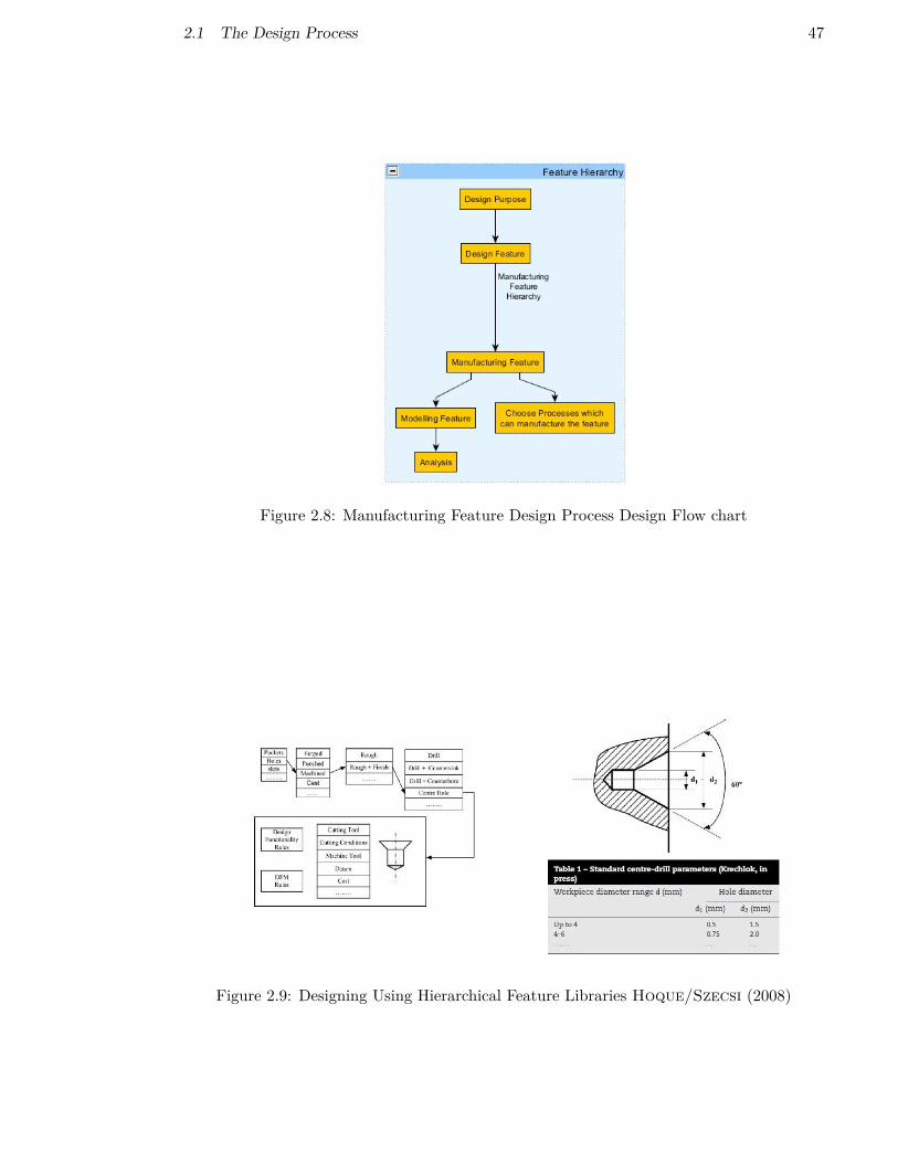
2.1 The Design Process 47
Figure 2.8: Manufacturing Feature Design Process Design Flow chart
Figure 2.9: Designing Using Hierarchical Feature Libraries Hoque/Szecsi (2008)

48 2 LITERATURE SURVEY
Figure 2.10: A design process where the computer selects the necessary design and manu-facturing feature according to designer’s declared intent
The primary issue with this approach is that the designer is expected to know which is theoptimal method to produce a manufacturing feature, which may not be the case foranything other than simple components.
The authors Brunetti/Golob (2000), of a system of feature library design, envisage thedata as being structured into four levels, the purpose and type of data within these levels isexplained below:
1. Assembly Model
(a) Contains the relationships between parts, and the reasoning behind it.
2. Part Model
(a) This level of model contains the data linking the component parts together, suchas welds or the data specific to the part such as material.
3. Feature Model
(a) Feature models contain the generic data necessary to reproduce the feature, butin addition the functional description of the feature, such as its connection toother features.
4. Generic Model
(a) Stores application data, this is data used to construct the model such as wouldbe stored in current CAD tools such as Solidworks or NX.
The system presented by Brunetti/Golob (2000) (Figure 2.10) allows the user topresent a problem to the computer, that is to say they will inform the computer what theywant to do, and the computer will then present a list of options, i.e. how this function can

2.1 The Design Process 49
be achieved. For example if two parts are to be joined together the computer will knowthey can be: welded, riveted, bolted, glued etc., and will suggest the different methodsaccording to the functional requirements such as heat conductivity, strength of join etc.This is in effect the opposite to that presented by Hoque/Szecsi (2008) because whilstHoque/Szecsi (2008) gives the user the opportunity to choose manufacturing methodsbased on experience and what they wish to achieve, Brunetti/Golob (2000) simplyrequest that the user specifies what they wish to achieve and the computer can analyse thedifferent methods of achieving it. This is advantageous because it means that the expertsin manufacturing methods need not be in the design team but can simply write the rulesthat the computer will use when presenting a list of viable options to the designer.
Ontological Conversion of Features Even if it is the case that the design featureswithin a part are known through manual construction by feature there is still therequirement to convert between design and manufacturing features. Design featurestypically have specific purposes and will still be present when the part is finished,manufacturing features however are simply a result of a manufacturing operation, whichmay or may not still be present in the finished part geometry.
Most feature recognition algorithms ignore this issue by recognising manufacturingfeatures, although of course any manufacturing features not present in the finishedgeometry (Section 2.1.3) are challenging.
Thus if feature recognition is not used there exist some methods of converting designfeatures to manufacturing features. One way is a simple mapping, the pre-specification of adesign feature as a combination of one or more manufacturing features. However, even ifthe mapping from one to many is simple the mapping of dimensions is not. One reason forthis is that due to the way that design and manufacturing are carried out. Designers willtypically think of features which achieve a purpose, whereas manufacturers think of how toachieve the feature, either using subtractive or additive/fabrication processes. These twopurposes require different dimensions for the same feature, either requiring somecomputational conversion rather than direct mapping of dimensions or a vastlyover-dimensioned design with both required design and manufacturing dimensions present.
A more advanced alternative to this simple mapping is the use of an ontology as proposedby Anjum et al. (2012), they use ontologies for the purpose of manufacturabilityverification but the approach can be adopted for cost knowledge purposes. The centralpremise behind their hypothesis is that design to manufacturing feature mappings can be:one to one, one to many, many to one and fractions in either direction, in additioncombinations of design dimensions may be necessary to obtain a single manufacturingdimension. Once they have obtained the manufacturing features they use a rules/logicbased approach to determine the manufacturability of the features. It should be noted thattheir approach is component specific and at this stage needs to be hard coded for each

50 2 LITERATURE SURVEY
component type with consideration for the tooling available in a specific factory. It wouldin theory be possible to make the knowledge more generic but this would come with a costof either more computation time expended, less accuracy or both.
Agyapong-Kodua System Agyapong-Kodua et al. (2012) have focussed on theneed for design for manufacture systems to take into account detailed information aboutthe capabilities for the company or supply chain they are being used for, in addition todynamic aspects such as resource availability. They also make the same point as haspreviously been made; this type of costing activity must be possible whilst the designdecisions are being made, if the costing activity is conducted later it is either too late or itlengthens unnecessarily the design time causing a loss of competitive advantage. They alsoconsider more business case decisions such as the make/buy choice but as with most of theliterature are unclear how exactly they generate the process sequence for manufacturingthe component.
DFM is part of a wider family of DFx methods reviewed by Agyapong-Kodua et al.(2013). They maintain that a design system should consider:
Design for:
1. Manufacture
2. Assembly
3. Maintainability
4. Environment
5. Quality
6. Decommissioning
7. Life-cycle
2.1.6 Value Driven Design (VDD)
Life-cycle methods including VDD (such as researched by Cheung et al. (2010); Zhaoet al. (2014)) encompasses all of the above DFx methods, in addition to the profitgenerated for the operator (which is a function of performance) or customer of the product(in this case a turbofan). This type of holistic approach is a requirement of VDD, wherethe value of a product to a potential customer is the revenue the product can generatesubtracting the cost. If a sufficient profit exists to compensate for the risk the potentialcustomer would be expected to purchase the product. For an evaluation of the value of aproduct however all costs and benefits must be known hence this research into a small

2.1 The Design Process 51
piece of this puzzle, the manufacturing cost. Once it is accepted that manufacturing cost isdesirable information at the same stage it must be accepted that it is worse than pointlessto know the manufacturing cost for a sub-optimal method of manufacture, this is whereprocess planning (Section 2.2) can be of use.
2.1.7 Summary of the design process
In summary the design process is continuously evolving, with more information availableearlier in the process enabling trade offs to be rationally made. This is allowing an everaccelerating design process and continual improvement in product performance, weight andcost. In order to remain competitive it is necessary to keep up with these trends and tocontinually conduct more analysis, earlier and with a greater breadth or exploration, lest asuperior solution be found by a competitor. Although not addressed in this research it isnecessary now to not only consider the cost of production of components, but to alsoconsider their maintenance, lifespan and decommissioning in a range of industries.
This requires detailed modelling of production costs, MTTF, decommissioning andrecycling costs in order to ensure a future loss is not made on today’s production. VDDattempts to quantify this.
As an addendum however it should be ensured that any change of activity (such as newproduction) can have a beneficial/deleterious effect on all existing production of a business.Thus if practical this should be analysed as well. A good example of this could be theintroduction of a new component into an existing factory, taking the factory over capacityand removing its resilience to unforeseen circumstances such as unplanned downtime.Equally the introduction into a factory operating below capacity can increase utilisationand thus reduce the costs of components already in production. These considerations aredefined as out of scope but are briefly commented on in Section 2.2.16.
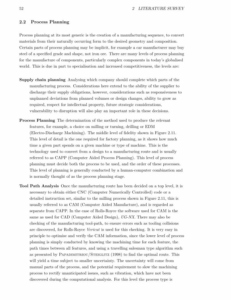
52 2 LITERATURE SURVEY
2.2 Process Planning
Process planning at its most generic is the creation of a manufacturing sequence, to convertmaterials from their naturally occurring form to the desired geometry and composition.Certain parts of process planning may be implicit, for example a car manufacturer may buysteel of a specified grade and shape, not iron ore. There are many levels of process planningfor the manufacture of components, particularly complex components in today’s globalisedworld. This is due in part to specialisation and increased competitiveness, the levels are:
Supply chain planning Analysing which company should complete which parts of themanufacturing process. Considerations here extend to the ability of the supplier todischarge their supply obligations, however, considerations such as responsiveness tounplanned deviations from planned volumes or design changes, ability to grow asrequired, respect for intellectual property, future strategic considerations,vulnerability to disruption will also play an important role in these decisions.
Process Planning The determination of the method used to produce the relevantfeatures, for example, a choice on milling or turning, drilling or EDM(Electro-Discharge Machining). The middle level of fidelity shown in Figure 2.11.This level of detail is the one required for factory planning, as it shows how muchtime a given part spends on a given machine or type of machine. This is thetechnology used to convert from a design to a manufacturing route and is usuallyreferred to as CAPP (Computer Aided Process Planning). This level of processplanning must decide both the process to be used, and the order of these processes.This level of planning is generally conducted by a human-computer combination andis normally thought of as the process planning stage.
Tool Path Analysis Once the manufacturing route has been decided on a top level, it isnecessary to obtain either CNC (Computer Numerically Controlled) code or adetailed instruction set, similar to the milling process shown in Figure 2.11, this isusually referred to as CAM (Computer Aided Manufacture), and is regarded asseparate from CAPP. In the case of Rolls-Royce the software used for CAM is thesame as used for CAD (Computer Aided Design), UG-NX. There may also bechecking of the manufacturing tool-path, to ensure errors such as tooling collisionsare discovered, for Rolls-Royce Vericut is used for this checking. It is very easy inprinciple to optimise and verify the CAM information, since the lower level of processplanning is simply conducted by knowing the machining time for each feature, thepath times between all features, and using a travelling salesman type algorithm suchas presented by Papadimitriou/Steiglitz (1998) to find the optimal route. Thiswill yield a time subject to smaller uncertainty. The uncertainty will come frommanual parts of the process, and the potential requirement to slow the machiningprocess to rectify unanticipated issues, such as vibration, which have not beendiscovered during the computational analysis. For this level the process type is
2.2 Process Planning 53
specified but the order of operations is yet to be decided.
Figure 2.11: A multi-level view of a hypothetical supply chain with times of processes
2.2.1 Supply chain modelling
Much progress can be made by improving the supply chain, although there is much debateon what, exactly, constitutes a “good” supply chain. There has been a shift, from largeindustrial companies in the developed world designing and manufacturing their ownproducts in their own country, to manufacturing their products in the developing world.Now, however, companies are subcontracting out the manufacturing, in an effort to reducecosts, as smaller, more specialised companies, can manage production more efficiently.There are two major disadvantages with this approach:
1. This lean supply chain can lack responsiveness in the event of unforeseencircumstances and the actions of competitors are more likely to disrupt it as supplierstend to supply more than one downstream business, this has in fact been one of thedriving forces for the process but can be deleterious during periods of high demand.
2. It has also led to a lack of knowledge about the cost drivers by designers. Designersknow how to improve performance but they do not necessarily know its effect on cost.A part is designed, and bids are accepted for contract work and so the knowledge ofcost drivers is not necessarily returned to the designers. This is to protect thesupplier’s intellectual property as a detailed cost model could be used to reverseengineer the production process.
One possible method of working around this issue of intellectual property is to solicit bidsfrom a number of different suppliers after design, as done by Marion (2008), where the
54 2 LITERATURE SURVEY
design was made available on the internet and suppliers were invited to bid for productionby offering contract terms. However, this is only really suitable for companies producingsimple products, where many suppliers have the capability to manufacture the product. Inthe aviation industry, due to the certification requirements, and the relatively smallproduction volumes (relative to, for example, the automotive industry) there are a limitednumber of suppliers. Finding new suppliers is also a costly exercise due to the auditingactivities involved. In addition, several design iterations are usually involved, and thesupplier is selected prior to the final design stage. Therefore this approach is unsuitable forthe high value or critical parts in aerospace industry. Some companies, includingRolls-Royce, are using cost modelling to predict how much supply chain componentsshould cost, thus their negotiators can enter into contract negotiation, with an expectationof the costs faced by their suppliers. This can be done using past experience and statisticalmodels, or by using generative cost models, however, it is just a prediction of whatsomeone (who is not the supplier) company thinks it should cost, and this method may notuse data directly from the manufacturer. In addition to the cost aspect of supply chains,one very important factor for the aerospace industry in particular, due to its long leadtimes and limited selection of suppliers, is risk. The issue of supply chain risk is focussedon in Ghadge et al. (2010) using a SoS (System of Systems) approach.
An article written by Pierreval et al. (2007) also engages in analysis of the supplychain. They use a continuous simulation approach, and logic to simulate the decisions ofdifferent sections of the supply chain. They have shown that continuous simulation can bea powerful tool, in anticipating and preventing issues such as supply shortages or increasedlead times due to insufficient capacities, and can thus be a useful tool when choosing ordervolumes, frequencies and stock levels.
2.2.2 An Introduction to CAPP (Computer Aided Process Planning)
Computer Aided Process Planning (CAPP) is a computational interface betweenComputer Aided Design (CAD), and Computer Aided Manufacture (CAM). CAPP isintended to be the process which makes all of, or a subset of decisions. Petrovi et al.(2015); Isnaini/Shirase (2014) carry out extensive studies on the process planningproblem, and generally agree on the necessary tasks a process planning system shouldperform, and what decisions it should be making. In particular they highlight the need forflexibility of operation choice, sequence, machine, tool and TAD and transportation costs.However, in addition to all of these, there is the consideration of fixturing/tooling, whichmay be a substantial portion of the cost.
The objective of CAPP is thus to construct a manufacturing process route which can beused to create a specific part within specified tolerances, however, there is discrepancywithin literature as to which of these decisions should be made within CAPP. For exampleresearch by (Yang et al., 2011; Razali, 2014) assumes that CAPP begins after the

2.2 Process Planning 55
choice of manufacturing processes. As will be highlighted throughout this section this isthe case with much literature, or the method of process selection is unclear.
There are several categories of CAPP:
Manual CAPP CAPP where a human is used to make decisions, based on informationand analysis provided computationally. In the opinion of the author these systemsare typically little more than advanced spreadsheets. Whilst they typically providean accurate answer for cost and production times among other data, the knowledge istypically less generic than in automated CAPP, and the routes generated by differentexperts are likely to differ. The results will often be sub-optimal but typically goodenough.
Singh et al. (2011) published an approach for the selection of a manufacturingstrategy or particular process. It relies on expert opinion to populate the matricessince they are filled with subjective opinion from a list of statements. It thenevaluates these matrices to obtain a best process, from the point of view of Quality,Cost, Capability and Production.
Automated CAPP CAPP where the human is not involved after prior programming ofdatabases or other knowledge repositories. This system requires computationaldecision making as well as cost and feasibility modelling. Automated CAPP comes intwo major sub-categories (Yusof/Latif, 2014a):
Variant Where the process route is the same as, or similar to, a previously usedmanufacturing route or route options.
Generative The process route is typically derived from some generic manufacturingknowledge, typically less accurate and more computationally expensive, butmore flexible than variant CAPP. The differentiating factor is that generativemethods generate a method of manufacture (MoM), whereas variant basedmethods use a pre-supplied MoM.
According to Xu et al. (2011) CAPP systems require manufacturing features to bedefined. However, it is more accurate to state that CAPP systems must either deduce themanufacturing features or they must be pre-defined. This is an important distinctionbecause manufacturing features will often be different from design features, particularlywhen designers add, for example, an extrusion to a part normally forged. A manufacturerwill think of adding extra material to the forging and then removing the extraneousmaterial with machining operations. Thus either manufacturing features must be usedduring design (Section 2.1.5) or there must be a method of converting from designgeometry to manufacturing features such as discussed in Section 2.1.4. In addition to thisthe design features may well be different from the modelling features used to constructthem (Zhou et al., 2007).
56 2 LITERATURE SURVEY
Several authors have defined process planning and stated what they believe the output of aCAPP tool should be:
“Process planning is defined as the activity of deciding which manufacturingprocesses and machines should be used to perform the various operationsnecessary to produce a component, and the sequence that the processes shouldfollow.” Marri et al. (1998)
“A detailed process plan usually contains the route, machine and tool,processes, and process parameters.” Marri et al. (1998)
“Systematic determination of the methods by which a product is to bemanufactured economically and competitively.” Culler/Burd (2007)
“Process planning deals with the selection of necessary manufacturing processesand determination of their sequences to ‘transform’ a designer’s ideas (namelythe designed part) into a physical component economically and competitively.”Xu et al. (2011)
This section of the literature review will focus mainly on the choice of manufacturing route,although certain parts of the literature are more broad ranging, such as Xu et al. (2005),which also encompasses feature recognition, CAPP and CNC code generation.
A CAPP tool such as that developed by Sadaiah et al. (2002), must determine whichprocess(es) and tool(s) to use for a given feature, and the order in which to perform theoperations. To determine the outcome of these choices, the geometric and toleranceinformation of the manufacturing features is typically used. Sequencing is usuallyimplemented through a set of constraints between pairs of operations. These constraintscan be stored in a number of ways such as matrices from Xu et al. (2005), or a list/tablesuch as that used by Salehi/Tavakkoli-Moghaddam (2009). It is interesting to notethat some authors sequence features prior to ascribing processes to those features whereassome simply keep the constraints and allow the optimiser to find a solution.
The manufacturing process is totally dependent on the forming process chosen for theinput material, although some parts of the process may be common to more than oneforming process. Kumar/Rajotia (2005) take this into account by using standard sizesfor axisymmetric components but of course the amount of material which must be removedis dependant on the difference between the forming shape and the finished part geometry.They also consider the power requirement of the tool to identify which machines arecapable of each operation.
A creator of a CAPP system must consider which decisions the system should be makingand how, what will be predetermined, and what will be left to downstream tools asoptions, explicitly or implicitly.

2.2 Process Planning 57
2.2.3 Knowledge Representation
A key factor in process planning (and generative costing) systems is the representation ofknowledge. In a costing system, the knowledge typically stored will consist of equationsused to calculate the times and costs of manufacturing processes as a function of geometry,material choice and tolerances. In a process planning system in addition to this knowledge,data on how to choose and intelligence on how to sequence the operations is also required.Consideration on how exactly to store this knowledge has been published byGrabowik/Knosala (2003). They, like most other researchers, have adopted a databasetype method because of its native ability to utilise complex query statements. Theyexplore how to deduce the set of manufacturing processes and tools selection necessary toconstruct a specific feature using expert knowledge encoded in a set of databases, optionsare suggested to the user who may confirm or change the selection.
Other researchers to recently use database knowledge for CAPP includes Jinks et al.(2010); Tammineni et al. (2009).
2.2.4 A Review of CAPP Methods
According to Marri et al. (1998); Culler/Burd (2007); Xu et al. (2011); Prakashet al. (2012); Yusof/Latif (2014b) there are multiple approaches to CAPP systems:
Manual A manual approach uses human judgement, to make decisions regarding whichprocesses, machines and tooling to use, and the sequence of the aforementionedprocesses. It typically results in a process plan similar to what would be produced bya variant based method. This is because humans are typically experience led, andthus more likely to choose a proven method over a novel, and possibly untested,methodology, provided the previous route is acceptable. There are many examples ofthis type of approach in the academic literature and in commercial use. In academiaa good methodology was presented by Wasim et al. (2013), which allowed the userto make the necessary choices, but also provided guidance on how well the route metvarious throughput, cost, strength and scrap rate metrics.
VariantBased A variant based approach is useful when there is a known process for aparticular component family, and this process can thus be replicated and modified (ina limited way) for other similar components. It typically involves interrogating adatabase after selecting the appropriate component family, and if necessary, subfamilies. For example on a component such as a gear with bolt holes, it is assumedthat holes will be drilled, and that this will occur at a certain point duringfabrication, the number of holes thus determines the cost of drilling them, there isvariation but no wholesale change to hardwired manufacturing routings. Thismethod is limited for novel components or changes in manufacturing process.
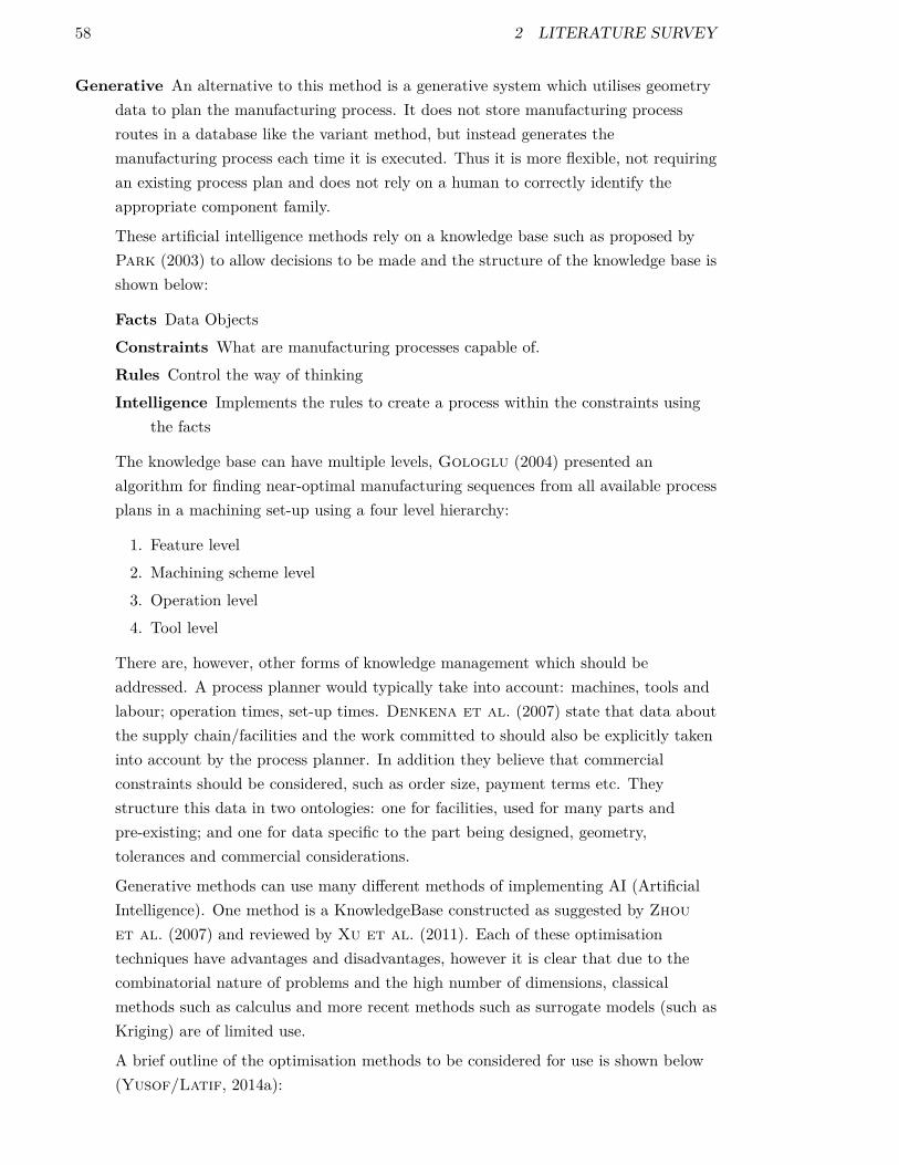
58 2 LITERATURE SURVEY
Generative An alternative to this method is a generative system which utilises geometrydata to plan the manufacturing process. It does not store manufacturing processroutes in a database like the variant method, but instead generates themanufacturing process each time it is executed. Thus it is more flexible, not requiringan existing process plan and does not rely on a human to correctly identify theappropriate component family.
These artificial intelligence methods rely on a knowledge base such as proposed byPark (2003) to allow decisions to be made and the structure of the knowledge base isshown below:
Facts Data ObjectsConstraints What are manufacturing processes capable of.Rules Control the way of thinkingIntelligence Implements the rules to create a process within the constraints using
the facts
The knowledge base can have multiple levels, Gologlu (2004) presented analgorithm for finding near-optimal manufacturing sequences from all available processplans in a machining set-up using a four level hierarchy:
1. Feature level2. Machining scheme level3. Operation level4. Tool level
There are, however, other forms of knowledge management which should beaddressed. A process planner would typically take into account: machines, tools andlabour; operation times, set-up times. Denkena et al. (2007) state that data aboutthe supply chain/facilities and the work committed to should also be explicitly takeninto account by the process planner. In addition they believe that commercialconstraints should be considered, such as order size, payment terms etc. Theystructure this data in two ontologies: one for facilities, used for many parts andpre-existing; and one for data specific to the part being designed, geometry,tolerances and commercial considerations.
Generative methods can use many different methods of implementing AI (ArtificialIntelligence). One method is a KnowledgeBase constructed as suggested by Zhouet al. (2007) and reviewed by Xu et al. (2011). Each of these optimisationtechniques have advantages and disadvantages, however it is clear that due to thecombinatorial nature of problems and the high number of dimensions, classicalmethods such as calculus and more recent methods such as surrogate models (such asKriging) are of limited use.
A brief outline of the optimisation methods to be considered for use is shown below(Yusof/Latif, 2014a):

2.2 Process Planning 59
NeuralNetworks Approaches which learn either over time or using a training set ofexamples to give a higher likelihood of selecting highly used outcomes.
GeneticAlgorithms Approaches which use quality based selection and propagationof superior solutions to converge to optimal answers through evolution.
AgentBasedMethods Methods which apply intelligent agents, often competingwith each other in decisions.
STEPCompliantCAPP CAPP which has two way compatibility with STEP, itcan use real factory data to modify its decisions and code (relies on suitablyequipped factories).
Graphical Algorithms Algorithms which make use of graphs and route planningmethodologies, such as travelling salesman problem solutions, to conduct theprocess planning task.
Simulated Annealing An addition to genetic algorithms which reduces theprobability or the selection of inferior individuals as the optimisation progresses.
Initially the author’s research will focus on genetic algorithms and agent basedmethods may need to be used to improve convergence of the algorithm in order toreduce optimisation time.
It is interesting to note that Park (2003) considers the fact that expert humans willquickly find solutions to a process planning problem by eliminating infeasible solutions. Ifthere is a computational way of eliminating swaths of the solution space, regions that areinfeasible or obviously suboptimal, then this should help to increase the execution speed ofthe algorithm. Also they consider how to store the knowledge of choices. They use theexample of a multi-diameter hole and use the concept of a final machining operation(which meets surface roughness and tolerance requirements) and pre-requisite operations toconstruct an operations list. It then constructs an order by using tool access requirements.
In addition it is useful to see that Lee et al. (2007) consider how to automaticallygenerate feature precedence relationships which are necessary due to material deformation,nested features or referencing. They then optimise based on tool access directions, there istherefore the implicit assumption that the task can be conducted on one machine and toolchange is less costly than part manipulation.
Another useful point of note is made by Han et al. (2001), who consider it necessary toconduct feature recognition and process planning together. Since unless all possible featurecombinations are output by the feature recognition algorithm, the process planner may beover-constrained and either find suboptimal solutions, or fail. It may fail because a featureinterpreted in one way, may give an unsolvable problem, due to constraints such asdeformation or access directions, whereas a different interpretation may give a feasiblesolution. Their algorithm constructs and evaluates all possible methods of making the setof features, and makes use of knowledge of the dimensions, tolerance and surface finish, of

60 2 LITERATURE SURVEY
the feature. It then applies the fact that certain operations such as reaming require otheroperations as prerequisites. Although all possible machining sequences are addressed inaddition to constraints at both the feature and operation level it appears from the articlethat the individual operation sequences to achieve the feature to the tolerance and surfacefinish requirements are hardwired based on Manufacturing Knowledge. It is also apparentthat emphasis is placed on handling time and machine/tool changes, rather than the actualmachining time for the feature. Finally it is unclear how additional/new processes wouldbe added to the database although it is assumed that the complete operation sequencewould be added, as an additional possibility. The algorithm attempts to minimise toolchanges, and the overall number of tools used. According to Xu et al. (2011) this enabledthe problem of operation sequencing to be systematically addressed.
Another approach to the problem of manufacturing process selection was presented byCheng (2011), who details the use of queries and formulae which can be used to determineprocess choice, feed rate and tool choice etc. This can replace the use of highly skilled andexperienced people for producing process plans for production. It is more detailed, but notas intelligent as other methods involving GAs presented earlier. Many methods now requirelittle or no human input during run-time but this still requires human input during theplanning process. This method, of course, requires high levels of maintenance, probably bypeople skilled in both manufacturing and coding but does have the advantage of reducingcomputational run time as the design search space is heavily restricted.
A more recent piece of research based on a similar concept which also allows theconstruction of multiple stages of manufacturing process for a single feature was conductedby Zhang et al. (2014), using Semantic Query-enhanced Web Rule Language (SQWRL).This is a powerful and expandable approach.
Additional research focussed on process planning focusses on integrating it with additionaltechnologies such as by Culler/Burd (2007) for factory simulation or Wang et al.(2013); Bettwy et al. (2014) for factory scheduling.
In some cases, authors of literature such as Zhang et al. (2008) allow the considerationof multiple factories, but there is no fundamental difference apart from the necessity toconsider transport costs. Profit margins can be considered as just a percentage change intime/volume based cost rates.
2.2.5 CAPP methods: Variant Method
One paper which incorporated CAPP using an assembly simulation was Culler/Burd(2007). Their platform is shown in Figure 2.12, however the process planning was limitedto the ordering of the processes. The choice of processes was predefined and the timesthereof was estimated by the Industrial Engineering function of Bombardier Aerospace.
2.2 Process Planning 61
Figure 2.12: The Delmia V5R15 Assembly Simulation in the Dassault V5 Platform(Culler/Burd (2007)) showing an optimiser complete with discrete event simulation.

62 2 LITERATURE SURVEY
Particular issues with the variant based approach are:
• The passage of time and progress of technology may have rendered the baseline[process plan] obsolete or suboptimal.
• The new component is sufficiently different from the baseline component to renderthe original process plan unsuitable (for example different material, geometry ortolerances).
• The baseline process plan may never, in fact, have been optimal and this is still notknown by the process planner.
2.2.6 CAPP methods: Infeasible solutions
It is likely to be the case that some features require others to be machined first. It isobvious for a human that finishing a face requires the face to be created first. Firstly theremust be a way or storing/deducing the precedence constraints such as the methodproposed by Zhou et al. (2007) which decides precedence based on:
Datum Datum features (used to locate others) are machined first
Family Parent features are machined before their children
Process Roughing features are machined before finishing
Concentration Concentrated similar features are machined together (this is not aconstraint but it is generally desirable)
Once these constraints are defined a methodology must be created to identify thesatisfaction or otherwise in a given process plan. If they are unsatisfied then according toSu et al. (2015) the main methods of solution are: repairing the process to a feasible oneafter generation and before/during objective function evaluation, or creating the processplan in such a way as to not create infeasible routes. It is a powerful approach but isunclear regarding the possibilities or selection of machines or tool access direction.
A combination of repair and graph based route construction was explored by Huang(2013) where the initial population contained only feasible routes by construction, ifinfeasible routes were created during recombination and mutation they were then repaired.It was limited to a single operation per feature.
2.2.7 CAPP methods: Genetic Algorithm
Some of the earliest proponents of the use of a Genetic Algorithm (GA) (Goldberg, 1989)to conduct process planning were Rocha et al. (1999), they attempt to minimise

2.2 Process Planning 63
manufacturing time whilst producing only feasible routes. As with many of the laterpapers, it is unclear how the operation list is generated, or whether the GA can addoperations. However, the authors do show that the selection of machines and tools, inaddition to the sequence of operations is controllable by GA chromosome modification.
Salehi/Tavakkoli-Moghaddam (2009) used a GA to optimise process plans for a partpredefined in terms of features.
The methodology they follow is:
1. The feasible sequences are created by GA
(a) By applying order constraints and clustering constraints
(b) Optimising for the maximum satisfaction of feasible constraints according to aweighting matrix.
(c) Each entry of the GA contains a feature number (as in 1, 2, 5, 4, 6, 3)
(d) Produces n feasible solutions for input into the next optimisation sequence.
The crossover operator used was developed by Gorges-Schleuter (1989) whichprevents the formation of illegal children from legal parents, an issue found with TSPtype GA solution methods. Mutation is conducted through an exchange operation.
2. The method then optimises, sequences, and selects which tool to use.
(a) Starts with the feasible solutions from the prior optimisation.
(b) This time each entry in the GA vector contains vectors/strings of machine, tooland TAD
(c) By applying additive constraints to feasible sequences.
The Crossover operator for this optimisation originated from a paper by Davis(1985) but has been developed for vector individuals.
An approach building on this was presented by Kafashi/Shakeri (2011), however, whilstthese algorithms are good at informing how to optimise a list of operations given a set ofconstraints, the arrival at the list of operations is ill defined. It appears to be based ontolerances and the type of feature, however, it is thought that they have created theoperations list, as shown in Figure 2.13, by using human knowledge rather than anautomated approach.
Amin-Naseri/Afshari (2012) build on the use of genetic algorithms, within a processplanning algorithm, by considering the scheduling problem posed by multiple parts passingthrough a factory simultaneously. They pre-calculate the operation precedence graph foreach job (component) and also pre-calculate the time of the operation for each potential

64 2 LITERATURE SURVEY
Figure 2.13: A list of operations used as the input to a GA optimiser routineKafashi/Shakeri (2011)
machine, they are also attempting to maximise throughput, a different objective function.In addition, they make several simplifying assumptions that are not made by this research:negligible transport and setup times, or at least independent of sequence, also processingtime is known and fixed.
They also convey a method of tuning genetic algorithm control variables developed byFranca et al. (2001), which is effectively derived from the Hooke and Jeeves numericaloptimisation method for functions. This methodology of holding all but one of theoptimisation variables constant and iterating over all variables is a simple and effectivelocal search to find the best parameters, although local optima in the parameter searchspace could be problematic and multiple problems must be tested to give the best generalparameters.
Another paper of particular interest is written by Wang et al. (2011). They also explorethe use of genetic algorithms but only for the evaluation of feasibility. They have not goneso far as to actually create the manufacturing route using backward and forwardpropagation and have not evaluated the sequence for cost, instead using a surrogate ofcomplexity. The chromosome definition appears elegant, although at a cost of flexibilityand expandability, and they have used crossover and a population. Furthermore they donot consider scrap/rework/tolerances and it is unclear how they handle crossover betweenchromosomes of differing length, in fact it is unclear that they allow them at all.Huang/Hu (2011) use a multi-level G.A. to select from a pre-defined set of manufacturingprocess chains for each manufacturing feature in an outer optimisation ring, then sequencesthem using graphical methods for satisfaction of constraints. As with many other papersthey do not consider costs apart from machining time, nor how to construct process chainsin-situ. Presentation of their results is also simple due to the fact that fewer costparameters are used.
Zahid/Baqai (2013) also explore the use of genetic algorithms to construct and evaluateprocess plans, their evaluation is limited to the consideration of setup and tool changecosts. They do highlight the option of reusing previously generated manufacturing routes

2.2 Process Planning 65
to accommodate new features, which could potentially be a useful addition, but it isunclear how they account for the potential to change the optimal manufacturing methodfor existing features.
Zhang et al. (2015a) highlight the issues of the distributed supply chain with manyoptions, i.e. the new opportunities when manufacturing is not constrained to a facility oreven a single company. They highlight the need for a more complex encoding ofindividuals, mutation operators which can operate on them and an efficient decodingmethodology in the objective function.
Xu et al. (2014) consider the creation of multiple stages for a single Feature MachiningElement (FME), however, they do not show how these stages are derived, or how the timesare calculated, i.e. fitness evaluation.
2.2.8 CAPP Methods: Graphical Algorithms
Graphical algorithms such as that proposed by Huang et al. (2012) work by constructingan operation precedence graph, and combining this approach with genetic algorithmoptimisation. The GA ensures optimisation whilst the graph exists to force feasibility. Thefeasibility algorithm used is iterative checking and switching of operations where aconstraint is breached, and they do not consider grouping constraints at all. This paperalso uses a repair function after each iteration, to ensure that all manufacturing sequencesare feasible. There is a stochastic method of machine and TAD (tool access direction)selection controlled by the central optimiser. Finally, it is clear that this tool is simply asequencing tool as no thought is given as to how to select the set of manufacturingprocesses or how to automatically create the process precedence constraints. Huang(2013) do begin to consider the selection of processes utilising their previously publishedgraphical approach (Huang et al., 2012), but they do not use the recursive propagationfound in other literature and this thesis (Section 2.2.10).
2.2.9 CAPP Methods: Simulated Annealing
Simulated Annealing (SA), as used by Lian et al. (2009), works by initially allowingfitness of individuals to decrease and thus allows exploration of the design space, butprogressively discourages descent to lower fitness (or ascent to higher energy states). It isbased on annealing in materials science by gradually reducing the thermodynamic freeenergy available to promote crystalline reorganisations. The particular strength of SA isthat the optimiser can traverse areas of decreasing fitness in order to find the globaloptimum whereas a pure hill climber requires a particularly fortuitous mutation to achievethis when there is high epistasis in the design search space. A GA (Genetic Algorithm)with SA was proposed by Lian et al. (2009) and was shown to be substantially better

66 2 LITERATURE SURVEY
than a GA without SA.
Lian et al. (2009) perform both manufacturing process selection and sequencing, theyconsider the type of operation, machine used, the tool access direction, and the specific toolused. They also perform an exhaustive search for each design feature to find all possiblecombinations of manufacturing processes, machine, TAD and tool. They have a repairalgorithm to find a feasible solution if one exists which operates by checking constraintsand moving a successor operation if it breaches a constraint to behind the predecessor.
Their hybrid algorithm essentially works by putting the best result from a GA generationinto the start point for SA. Only when the SA process plan is better than all the resultsfrom the GA is the SA algorithm used. Effectively the GA populates the start point for theSA algorithm the SA can be seen as a local search which is not always a hill climber,though its propensity to descend to lower fitness values reduces as time progresses.
2.2.10 CAPP Methods: ANN (Artificial Neural Network)
Zhou et al. (2007) proposed a method based on backward propagation (BP), to create alist of processes and constraints, then using a GA to optimise the sequence. Theconstraints include datum precedence, feature precedence and process precedence althoughit could be argued that datum precedence is simply a sub-category of feature precedence.
The way that BP works, in detail, is the algorithm selects a manufacturing process for afeature based on a trained ANN (Artificial Neural Network), and then works back throughthe processes necessary as pre-requisites, according to probabilities which are known by theneural network from training, by manufacturing process experts. This builds on the workby Park (2003), which uses the concept of a final machining operation using tolerance andsurface finish requirements.
In addition, the algorithm takes into account machines, machine cost rates, tools, tool costindices, and tool access directions.
Khalifa et al. (2006) suggest the use of neural networks for the selection of machinetools, it is possible that a neural network approach could be used, either within theoptimiser to learn over time, or with an external data input, to improve the convergencerate. Bringing the neural net inside the optimiser and making it learn which manufacturingprocesses are used most frequently for specific features would also further differentiate thework from Zhou et al. (2007), who used a pre-populated neural network.

2.2 Process Planning 67
2.2.11 CAPP Methods: Logic and Query based
In addition to the aforementioned optimisation based methods above, Grabowik et al.(2005); Zhang et al. (2010) and others have promoted logical methods of processselection. This will optimise a component on a feature by feature basis, which may resultin a globally sub-optimal solution. It will, however, be much faster and potentiallysufficiently good for industrial applications. This type of method requires far moreextensive calibration of the database as rules must be coded rather than simple options.Given the speed of this type of approach Grabowik et al. (2005) incorporated with it asequencing planner designed to react to disturbances, for example an offline machine.Their system could quickly re-route a component to minimise the loss of output byselecting alternative manufacturing methods or sequences. The methodology used byaPriori (Section 3.2) uses logic and query based methods.
2.2.12 CAPP Methods: Other
Other methods have been developed for optimisation of the manufacturing route.
One of these was developed by Lv/Qiao (2013), who construct an AND/OR graphdetailing the manufacturing routes, and machine possibilities, for each manufacturingoperation. This graph can be manipulated to give all feasible sequences, but it is thisauthor’s belief that with the levels of complexity dealt with in this research the graphwould not only be unintelligible, but excessively computationally complex to create. One ofthe aspects that they do consider however, which is dealt with differently in this research,are the intra-factory transfers. Using a machine list they specify the transport timesbetween all pairs of machines, the times are, however, independent of the current value andmass of the component.
Another method, by Prakash et al. (2012) used a Knowledge-Based Artificial ImmuneSystem (KBAIS). They considered the re-sequencing of a series of operations where the setof operations was fixed, but the order was not, and the machine, tool and TAD choice wasalso made by the optimiser from a pre-defined list. In addition they claim novelty inconsidering scrap to be a factor of which machine was chosen and calculating the costs onthis basis.
Tabu searches have also been explored by Li et al. (2003) for the CAPP optimisationproblem as a way of escaping local minima as an alternative to simulated annealing, Tabusearch can be considered an extension to simulated annealing optimisation.

68 2 LITERATURE SURVEY
2.2.13 Difficulties with CAPP
Issues with CAPP software tend to be incompatibility of data structures; some of this isdue to fundamental differences between the way that designers design components and theway they are made. Due to various factors including structural requirements, it is often thecase that components start as a forged CoS (Condition of Supply) and are machined downto the correct dimensions. Thus manufacturers tend to think in terms of forming andsubtractive mechanisms whilst designers may think of additive processes, for exampleadding an extra feature. In some cases such as slots or holes a designer may think in thesame way as a manufacturer, but this is not always the case.
Despite much progress in understanding how to model the CAPP process, and informationflows which are necessary, there has not been as much progress on the actual integration offully automated Process Planning systems. According to Zhou et al. (2007) this is inpart because of the difficulty in converting CAD features to manufacturing features. Zhouet al. (2007) propose feature recognition as a solution to this and have implemented thissolution in UGS/SolidEdge.
The reason Zhou et al. (2007), do not favour manufacturing feature based design is thesame reason stated by Scanlan et al. (2006), namely it would restrict the designers andprevent interesting and potentially useful experimentation because they cannot (or it isdifficult to) create unusual parts in their design tool. The other issue, according to Zhouet al. (2007), with feature based design is that intersecting features which may beseparate in a feature based design tool may actually combine as manufacturing features.
Thus they favour feature recognition despite the current limitations, particularly issuesresulting from the storage of data on tolerances, surface roughness and hardness, which canaffect manufacturing cost substantially, affecting machining time and the process which canbe used. One way of extracting this non-geometric data, presented by Prabhu et al.(2001), is using natural language processing intended to read the notes intended for humaninterpretation from the model file, and combining them with features before the data isoutput as a part model. Features are then defined together with their GD&T (GeometricDimension and Tolerance) information. The way the text is matched with the appropriatefeature involves the use of recognition of arrows and the location using encoded logicwithin the programming rather than artificial learning techniques such as neural nets.Another way of storing the information, which also takes into account the “datum story”was explored by Shah et al. (1998) by storing the GD&T information within a featurebased design model. It decomposes dimensions and tolerances into three dimensions anddeals with each separately. Thus, provided it is aware of the tolerances and what theymeasure, it can calculate, in principle at least, the ultimate deviation of a feature. Thistype of approach may also be useful when calculating material removal volumes ofintersecting features.

2.2 Process Planning 69
Issues with a GD&T system are difficulties in making it suitable for both CAD and CAPP.This is the essential difficulty in comparison between design and manufacturing features asoutlined in Section 2.1.4, since the simplest way to design a feature is rarely the simplestway to manufacture it. The further challenges posed by feature extraction according toZhou et al. (2007) are:
1. Recognition of intersecting features.
2. Handling multiple interpretations of features that correspond to different ways tomachine the part and therefore provide downstream applications with addedflexibility.
3. Controlling computational complexity.
4. Feature constraint extraction.
5. Feature precedence tree reconstruction.
2.2.14 ASP (Assembly Sequence Planning)
A subset of problems within process planning is assembly planning. It is related in thatjoining methods must be chosen and sequenced, and the criteria are similar: to meet thedesign specifications as cost effectively as possible. The issues are normally accessconstraints or difficulties, weld deformation, join strength and access for later maintenance.
According to Yu/Wang (2013), ASP is generally conducted by ACO (Ant ColonyOptimisation), GA (Genetic Algorithm) or PSO (Particle Swarm Optimisation). Theirchosen approach of ACO works by encouraging the use of well-travelled paths, althoughthe algorithm was adapted to maximise computational efficiency. ASP generally requiresknowledge of access difficulties and the authors differentiate between functional componentsand connectors, connectors are purely in existence to locate the functional parts. Theymaintain that this algorithm does take care of subassembly problems, but it is unclear how.One major issue of process planners for assemblies is when are manufacturing operationscarried out, if they could be done before or after assembly operations. This occurs whendesign features are still accessible after assembly operations, indeed to ensure continuity ofthe surfaces and structural rigidity during assembly it may be desirable to conduct someoperations afterwards. However, this question is incredibly difficult to formulate and addsanother layer of complexity to a problem which is already computationally challenging.
The algorithm Yu/Wang (2013) propose essentially attempts to minimise changes inorientation and will try to group similar operations together but taking into account hardconstraints such as access but also the softer constraints caused by friction and ease ofassembly, a solution worthy of consideration.

70 2 LITERATURE SURVEY
Esterman Jr/Kamath (2010) also propose metrics for the improvement of the assemblysequence. Firstly they consider the optimum planning of an assembly line with regards tothe number of workstations and operators, they then consider the potential improvementby relaxing precedence constraints, that is to say component redesigns which makealternative assembly sequences feasible. They analyse the assembly sequence with theobjective to improve: a) assembly time, or b) load balancing.
A particularly large assembly planning problem in the shipbuilding industry was exploredby Iwakowicz (2016), they use precedence constraints and a genetic algorithm to explorethe design space in order to minimise the assembly time.
2.2.15 Process selection and sequencing
The processes which can be used to produce a given feature are dependant on the factorsdiscussed in Section 2.3. Thus if this information is in the design system, the design systemcan identify which processes can be used to produce feature x. Some of the manufacturingoperations will be due to features which exist in the drawing, however some are due toother operations. For example a weld operation which will appear in the drawing mayresult in mandatory full x-ray checking of weld lines. Many machining operations aresubject to dimensional inspection, but wouldn’t be if the machine had an independentposition checking probe, since it could check dimensions at the same time as the machiningwere occurring and thus correct under machined defects before the component leaves themachine. It is also clear that an inspection operation would necessarily be following themachining operation which it is inspecting so the approach taken by Sormaz et al. (2010)is to keep the machining and inspection as a single part activity which requires multiplemachine activities. They also mention the fact that machine cells are normally configuredto minimise inter-cellular transfers, however, this is not necessarily always the case. Wherethe cost of inter-cellular transfer is only slightly more than intra-cellular transfer andmachinery can be run by a partially absent operator it may be more sensible to minimiseoperator movement, thus reducing the employee numbers necessary to operate the factory.
2.2.16 Production planning (Scheduling)
It is worth noting that the process planning task cannot be completely isolated fromproduction planning, and in an ideal world they would be optimised together(Zhang/Wong, 2015; Bettwy et al., 2014). Leus et al. (2014) in particular highlightthe benefit of similarity between product lines and create a method whereby manufacturingroutes for multiple components undergoing simultaneous production can be optimisedtogether to minimise total cost. The optimal process plan should take into account theavailability of the machines and labour required to conduct the manufacturing.Additionally, in an ideal world the process plan of any/all existing components passing
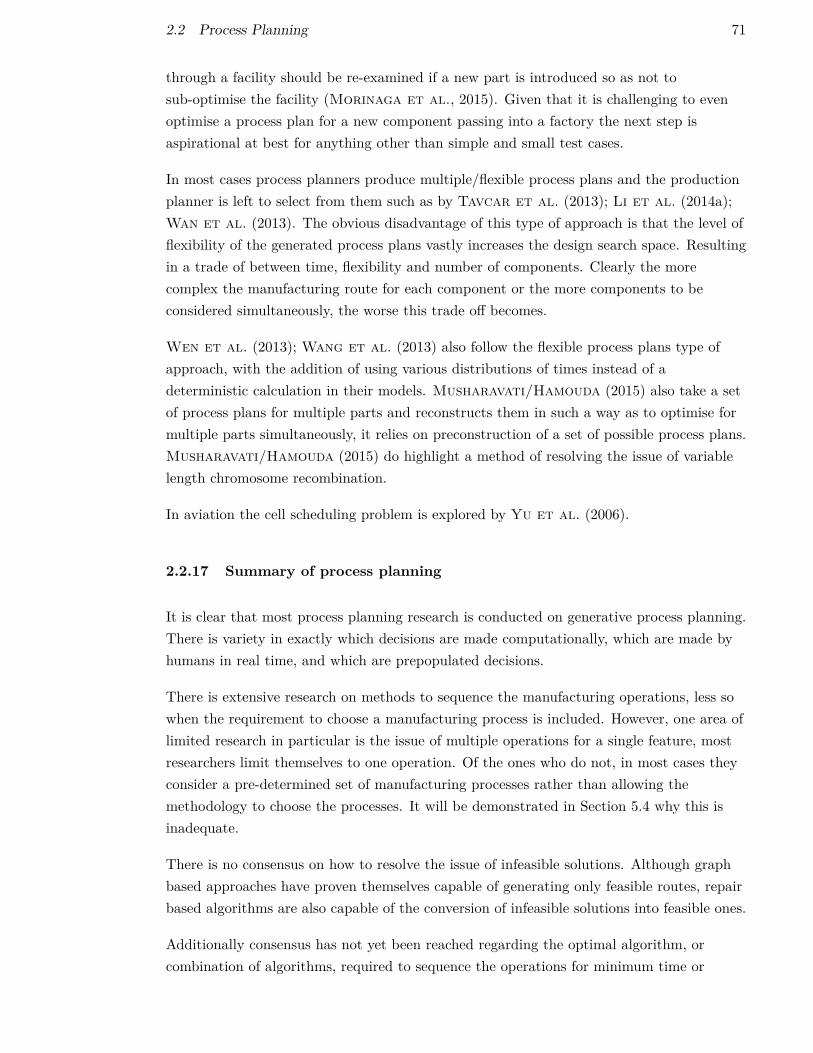
2.2 Process Planning 71
through a facility should be re-examined if a new part is introduced so as not tosub-optimise the facility (Morinaga et al., 2015). Given that it is challenging to evenoptimise a process plan for a new component passing into a factory the next step isaspirational at best for anything other than simple and small test cases.
In most cases process planners produce multiple/flexible process plans and the productionplanner is left to select from them such as by Tavcar et al. (2013); Li et al. (2014a);Wan et al. (2013). The obvious disadvantage of this type of approach is that the level offlexibility of the generated process plans vastly increases the design search space. Resultingin a trade of between time, flexibility and number of components. Clearly the morecomplex the manufacturing route for each component or the more components to beconsidered simultaneously, the worse this trade off becomes.
Wen et al. (2013); Wang et al. (2013) also follow the flexible process plans type ofapproach, with the addition of using various distributions of times instead of adeterministic calculation in their models. Musharavati/Hamouda (2015) also take a setof process plans for multiple parts and reconstructs them in such a way as to optimise formultiple parts simultaneously, it relies on preconstruction of a set of possible process plans.Musharavati/Hamouda (2015) do highlight a method of resolving the issue of variablelength chromosome recombination.
In aviation the cell scheduling problem is explored by Yu et al. (2006).
2.2.17 Summary of process planning
It is clear that most process planning research is conducted on generative process planning.There is variety in exactly which decisions are made computationally, which are made byhumans in real time, and which are prepopulated decisions.
There is extensive research on methods to sequence the manufacturing operations, less sowhen the requirement to choose a manufacturing process is included. However, one area oflimited research in particular is the issue of multiple operations for a single feature, mostresearchers limit themselves to one operation. Of the ones who do not, in most cases theyconsider a pre-determined set of manufacturing processes rather than allowing themethodology to choose the processes. It will be demonstrated in Section 5.4 why this isinadequate.
There is no consensus on how to resolve the issue of infeasible solutions. Although graphbased approaches have proven themselves capable of generating only feasible routes, repairbased algorithms are also capable of the conversion of infeasible solutions into feasible ones.
Additionally consensus has not yet been reached regarding the optimal algorithm, orcombination of algorithms, required to sequence the operations for minimum time or

72 2 LITERATURE SURVEY
minimum cost. Although genetic algorithms, frequently combined with other methods,have shown promise.
In terms of the selection of machines during the process planning the most powerfulmethodology was created by Zhang et al. (2014), their use of Semantic Query-enhancedWeb Rule Language allows vast flexibility in the conditions applied to choices, such asmachine or tool choices.
The area of compound scrap and its incorporation into process planning has not beenexplored adequately.
The issues of assembly sequence planning are defined as out of scope in order toconcentrate on component manufacturing, equally the dynamic aspects of productionplanning are disregarded.

2.3 Integrating CAPP with CAD 73
2.3 Integrating CAPP with CAD
CAPP generally requires more data than CAD, particularly information about tolerancesand surface finishes. In addition, CAPP is generally conducted using manufacturingfeatures whereas CAD generally uses design features (either explicit or implicit within themind of the designer). Therefore in general it is necessary to convert the data. This can bedone either using structured data and a translator or feature recognition, or a combination.Proponents of the latter include Kang et al. (2003) who propose neutral file formats forthe interlinking, particularly the STEP AP formats. Proponents of the former such asLeo Kumar et al. (2015) use XML and feature based modelling, to avoid the need forfeature recognition, and attempt to combine this data with a knowledge based system,however, their research is limited to prismatic micro parts.
There is also much research modelling the process by which the linking should be done.According to Feng (2003), several process models are available which describe how toproduce manufacturing process planning data, there are several pieces of informationgenerically necessary to select a manufacturing process:
1. Product Model Data
(a) Geometry
(b) Material (including necessary treatments such as nitriding, carbiding or shotpeening)
(c) Tolerance
(d) Surface Properties
2. Process Related Data
(a) Manufacturing Resource Availability
(b) Process Capability Specification
A significant number of the models reviewed use the IDEF0 modelling language, whichdescribes the necessary information inputs to a task, the control mechanism, the resourcesnecessary to complete the task and the information it provides. It can thus be used inhierarchy form by decomposing activities into sub-activities multiple times, which is anessential requirement in complex process planning for human interpretation. Howeveralthough it describes the actions and information necessary for a complex activity it doesnot necessarily detail how it can be done.
The modelling that Feng (2003) conducted does covers both CAPP and CAM as it:
1. Takes CAD data

74 2 LITERATURE SURVEY
2. Derives machining features
3. Process plans the manufacturing route (considering feature type and tolerance)
4. Process plans the factory floor route (Given the options available for manufacturing,on which workstation should the operations be completed on.)
5. Creates NC programs
6. Checks NC plans
It is said by Zhou et al. (2007) that most researchers use neutral file-based solutions toaddress the issue of the transfer of data between CAD and CAPP and CAM. The data istransferred using STEP (simple ASCII coded files) or IGES (Initial Graphics ExchangeSpecification) files (which are also ASCII encoded) to transfer data, although XML hasbeen used more recently, notably by Sormaz et al. (2010). The difficulty with this isthat the communication is usually one-way, thus a separate method is necessary to givefeedback to the designer.
Zhou et al. (2007) follow a several step process.
1. Get modelling feature F0, from the CAD tool
2. Convert to design feature FD, through a feature recognition algorithm.
3. Convert to manufacturing feature FM , which could take one of two forms:
(a) Form Features: Pre-defined features such as holes and slots etc. with analyticallycalculable material removal volumes and associated manufacturing methods.
(b) Surface features: Refer to surfaces which are not part of a recognised formfeature.
4. Manufacturing Process selection
5. Operation Sequencing
The way that Zhou et al. (2007) choose manufacturing processes when more than one isavailable to machine a feature is a back propagation Artificial Neural Network (ANN). Thisrelies of course on knowing the final finished form of the component and expert evaluationof data sets for neural network training according to:
• Feature
– dimension
– tolerance and
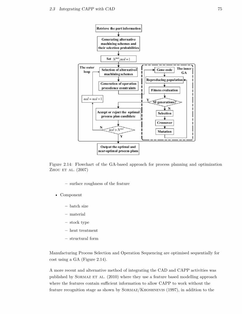
2.3 Integrating CAPP with CAD 75
Figure 2.14: Flowchart of the GA-based approach for process planning and optimizationZhou et al. (2007)
– surface roughness of the feature
• Component
– batch size
– material
– stock type
– heat treatment
– structural form
Manufacturing Process Selection and Operation Sequencing are optimised sequentially forcost using a GA (Figure 2.14).
A more recent and alternative method of integrating the CAD and CAPP activities waspublished by Sormaz et al. (2010) where they use a feature based modelling approachwhere the features contain sufficient information to allow CAPP to work without thefeature recognition stage as shown by Sormaz/Khoshnevis (1997), in addition to the

76 2 LITERATURE SURVEY
feature model however they believe it is necessary to maintain a solid model for geometricanalysis and the geometric model would be required in any case for analysis such as FEAor CFD. Sormaz/Khoshnevis (1997) also have a feature precedence network (FPN) toaid in the sequencing of operations. Some operations can be performed in any order but insome cases, either because of access or other constraints some features must be machinedbefore others. In addition to a feature precedence network they use a manufacturingprecedence network to denote which order manufacturing processes can/must be used, forexample hole starting drilling is necessary before drilling and then finishing the hole.
2.3.1 Summary of CAD-CAPP integration
Feature recognition or design by feature (in their broadest sense) are clearly the onlyalternatives which exist for converting design geometry into the features necessary forprocess planning. They both have issues, feature recognition mainly with intersectingfeatures and design by feature with the potential for reduced design flexibility if insufficientfeatures are defined.
This area will be defined as out of scope and design by feature will be used to provide ageometry driven input to the process planning methodology developed.
It is also worth highlighting that geometry is not the only required input to processplanning; material choice, production volumes, date of commencement of production andtype of part are also important factors, although this is not an exhaustive list.

2.4 Prediction of precursor shape 77
2.4 Prediction of precursor shape
It is noteworthy that a fundamental consideration in process planning is the question“what do I start with?”. Without an answer to this question, only the times of processesindependent of volume can be predicted, and these are few and far between. As stated byMasel et al. (2010), there are several classes of methods to predict the forming shapeand these will be outlined below:
Intuitive An expert, potentially assisted by a computer program (Caporalli et al.,1998; Gronostajski et al., 2015), generates the forging shape. Therefore (Maselet al., 2010) these are semi-automated systems such as outlined byBISWAS/KNIGHT (1976), including: Cubic Splines, exponential functions andgeometric transforms.
Analogical
Expert An expert, potentially assisted by a computer, generates the forging shapeusing past designs.
ANN An artificial neural network can be trained on a set of data to recognisepatterns, and derive forging shapes for new components. However Masel et al.(2010) highlight the fact that if the ANN is exposed to a class of component notencountered in the training set, it may give an inaccurate or unrealistic reponse.
Parametric Using parametric rules the forging shape is designed, and constrained to theshape of the finished part geometry. Examples could be:
Face-line offset A simple offset which assumes a simple, fixed, offset of n mm to aface (3d) or line (2d) Toal (2012).
Smoothed Similar to above, but ensures a smooth shape without low radius curvesToal (2012).
Analytical Using rules, but at a more detailed (feature based) level, the forging shape isestimated, and responds to the shape of the finished part geometry. Can be moreflexible than parametric methods, but requires more time and expertise to build ageneric rule set.
Rules Based Generally more accurate than the above (parametric methods), butrequires generation of a rule set such as outlined below, in order of ascendingcomplexity and usefulness:
• This can be for a specific component type such as high pressure compressor disk.This has been completed by Meas (2015).
• A more generic rule set which could work on component class such as disks.This has not been found in the literature.

78 2 LITERATURE SURVEY
• A truly generic rule set which could work on any component geometry. This hasnot been found in the literature.
Simulation An analytical type of approach where instead of rules applied togeometry, a flow simulation is created. An example of this was published byCaporalli et al. (1998). They use Ansys (v5.3) to simulate the metal flow,however, as they state, the system relies on experts to modify the forging andprocess sequence.
There are also two different levels of rules based methods in the literature: simple rulesapplied consecutively to the finished shape and, more frequently, simulation based timedependant finite element flow models, to predict detailed mechanical properties of theforged component.
A simple rules based approach was presented by Masel et al. (2010). They developedthis methodology to provide a rapid estimate of forged shapes, and therefore cost of theforging, since they state existing methods were extensive computational exercises. Existingmethods, they claim, were designed for detailed design of die shapes, making themunsuitable for iterative design work. Their method relates only to axisymmetric shapes,and relies upon knowledge of the finished part geometry. The rules are relatively simple andapplied sequentially, but need to be coded for each manufacturing strategy. The resultantvolumes do correlate strongly to known forging volumes from a sample of parts, but it isthought that a more generic method is desirable than one specifically designed for forging.No mention is made of its accuracy, when applied to other manufacturing strategies.
A detailed thesis into a rules based approach for blisks and discs, which was patented andadopted by Rolls-Royce plc, was written by Meas (2015), in which he highlighted thedifficulties in accurately predicting the forging shape. His methodology centered aroundcreating an ultrasonically inspectable Condition of Supply (COS), and from that derivingan appropriate and accurate isothermal black forging shape, from which the COS could bemachined. The methodology behind the creation of the black forging shape was tosequentially apply rules (obtained from Semiatin (2005)) to the COS shape until all ruleswere satisfied.
The rules applied were drafts, corners and fillets, webs and ribs, flash and trim. A diagramof the process used by Meas (2015) is shown in Figure 2.15.
One of the factors of interest is that Semiatin (2005) showed that parameters such as filletradii are material dependant. This will have an effect on precise design but not necessarilya significant effect in early design, when more inaccuracy is present in other factors.
Papers presenting forging shape prediction methods using detailed simulation include thoseby Kulon et al. (2006); Bramley/Mynors (2000); Biba et al. (2001). Biba et al.(2001) highlight the importance of disallowing the user from adjusting parameters of the

2.4 Prediction of precursor shape 79
Figure 2.15: The approach used by Meas (2015) (Figure 51) to predict forging shape froman ultrasoncially inspectable COS
simulation, thus preventing the quality of its outputs becoming dependent on the skill ofthe user, but only the quality of the software. Masel et al. (2010) similarly mention thedisadvantages of allowing an expert to vary parameters in terms of the inconsistancy ofresponses.
The more detailed simulation models could in principle be used to estimate the formingshape, to feed into cost modelling, but to obtain an accurate result they generally requiresignificant computational time. Equally a relatively simple rules based approach such aspresented by Masel et al. (2010) could be used, however this approach is currentlylimited to forging discs and blisks. Thus this research will attempt a new method, to beexplained in Section 4, in an attempt to reduce the necessary maintenance of the models.The methodology will attempt to provide estimates for a range of forming processes, notjust limited to forging.
80 2 LITERATURE SURVEY
2.5 Manufacturing Processes
It can be said that in the past manufacturing was generally a subtractive process,particularly in load bearing components so a manufacturing engineer will generally think interms of starting with more raw material and subtracting the sections which areunnecessary. However, a designer can use either additive (extrusion) or subtractive(shelling or lofting) methods to achieve the desired shape. In addition, modern methods ofmanufacturing can include additive processes and more advances methods of forming suchas powder bed forming, which should be considered by a process planner.
Additive manufacturing using material deposition is possible, as used in rapid prototyping,and a recent development was published by Karunakaran et al. (2010), the authorsused a CNC milling machine retrofitted with a weld deposition capability, thus bothadditive and subtracted processes can be used in sequence. Although as stated by Skibaet al. (2009) the structural properties of additive processes may be inferior to those ofcast or forged components due to factors such as HAZ (Heat Affected Zones).
There are many types of manufacturing processes, and they can be generally classified intoseveral categories: material removal; material forming; joining; clean up; surface treatmentand inspection.
Another useful way of looking at some of the manufacturing processes is through ahierarchy as created by Sormaz et al. (2010), which has been expanded and is shown inFigure 2.16.
2.5.1 Material Removal
Material removal generally consists of multiple stages. Primary (or rough) machining withhigh material removal rates, then fine machining with lower material removal rates andhigher tooling costs for finishing work due its superior surface finish and reduced processvariability. A large amount of material may be wasted although much of it can be recycled.
1. Turning is a tooling intensive operation, particularly on hard materials such astitanium.
2. Milling machines have a lot of wasted time due to tool changes or CNC manipulationof components. They are also intrinsically slower due to the method of forceapplication; a direct result of the shapes they are designed to machine.
It is possible to obtain mill-turn machines which would reduce the set up time as they canperform both operations but they are more costly than each of the two individual machines.
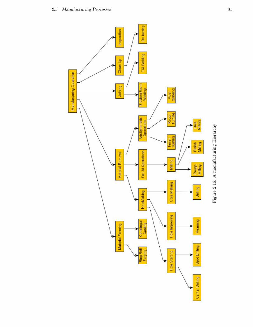
2.5 Manufacturing Processes 81
Figu
re2.16
:A
man
ufacturin
gHierarchy
82 2 LITERATURE SURVEY
Material removal processes are normally followed by a dimensional inspection and clean-upoperations such as deburring.
2.5.2 Joining (Welding)
Electron Beam Welding is used for high quality welding of titanium. Machines canautomatically track the join lines, manipulate the object being welded, perform bothstructural, cosmetic, penetrating and non-penetrating welds. However their limitations canbe weld angles, beam dumping requirements, spatter (particularly at high power), they alsoinduce high latent stresses in the component (though only on a very localised area), andcause consistent distortion of the component.
TIG (Tungsten Inert Gas) welding is a manual process, inexpensive and results in goodquality cosmetic welds and no weld spatter but the process is slow and results forstructural welds can be inconsistent, depending on the skill of the welder. There is also arelatively large heat induced stress zone because the weld rate is slow.
The welding process involves assembly, welding, clean up and an x-ray inspection of aproportion of the total welds, the extensiveness of the inspection depends on the criticalityof the component.
2.5.3 Manufacturing processes modelling and optimisation
There has been much research specific to one type of manufacturing process, to understandthe process, model it and in some cases optimise it. This aspect of research is defined asout of scope but this type of approach in optimising individual manufacturing processesshould contain/create models which could be data-mined to produce the equationsnecessary for input into other methodologies such as presented in Section 5.
For some forming processes a major contribution to the cost on low volume production isthe cost of manufacturing the dies, this is particularly applicable to components forged ofextremely hard materials/high temperature materials such as nickel molybdenum alloyswhich are required for the high temperature and high stress areas of missiles and gasturbines. The work published by El-Mounayri (1997) could be used for this purpose toestimate the die production cost, which could then be amortised over the expected lifetimeto improve the accuracy of the forming process cost modelling.
Some modelling research into forming processes is exemplified below.
• Forging by Behrens et al. (2011); Gronostajski et al. (2015)
• Centrifugal casting

2.5 Manufacturing Processes 83
• Die casting
• Power HIP (Hot Isostatic Pressing)
• Zhu et al. (2012) for continuous casting
• Park et al. (2006) for composite manufacture
• Taufik et al. (2011) for MMC (Metal Matrix Composite) manufacture
• AML analysis by Thomas et al. (2016); Zhang et al. (2015b)
Subtractive manufacturing processes have also been explored
• Chiu/Weigh (2012) used them to optimise micro-milling
• Laser based processes have been explored by Wiedenmann/Zaeh (2015)
• Milling processes by Leo Kumar et al. (2014); Li et al. (2014b); Ouyang (2015)
• Drilling by Li et al. (2015)
• Optimisation of Electro Discharge Machining (EDM) byAzadi Moghaddam/Kolahan (2015)
• Tolerance and cost of Electrochemical Machining (ECM) is analysed by Ayyappanet al. (2015)
• Turning Sortino et al. (2015)
Finally joining processes
• Linear friction welding Tao et al. (2008)
The detailed optimisation and analysis of individual manufacturing processes is out ofscope of this research. This type of approach in optimising individual manufacturingprocesses should contain/create models which could be data-mined to produce theequations necessary for input into other methodologies such as presented in Section 5.
2.5.4 Fixturing
It is noted from the research of Ribeiro et al. (2012) that tooling design andspecification can have a significant effect on the processing time during manufacture andthus a trade off can be made between unit cost and non recurring costs (NRCs). Generallythe more capable the fixturing is, the faster the part can be manufactured in general(provided that component deformation during machining is the limiting factor, often the

84 2 LITERATURE SURVEY
case in aerospace applications). However, a more capable fixturing is generally morecustomised, and less reusable, and thus the non recurring costs must be amortised over asmaller number of parts.
Equally a more capable fixturing system can be developed such as by Nasr et al. (2015)but of course this requires reconstruction to be changed from one fixture design to another,i.e. the setup costs may be raised at the end of a batch of parts to convert from one toanother.
The methodology this thesis describes could take this effect into account through multipleapproaches but it is left to future work for this to be implemented.
2.5.5 Summary of manufacturing processes
Limitations of manufacturing processes can be used to identify which processes can be usedto create certain features and tolerances combined with process variability will thendetermine the probability of successfully creating the feature(s).
From the point of view of cost, the manufacturability of components is highly important.Work by authors such as Sanz-Lobera et al. (2015); Dodd et al. (2015) reviewedexisting methods and presented proposals on functions to predict the effect of changingtolerance on the manufacturing cost of a component.
In addition the research conducted on manufacturing processes can be used for thepurposes of modelling their cost. Either directly or indirectly if the research proposes timegeneration models. In some ways time generation is better, given that it allows the user ofthe model freedom to set their own cost rate assumptions, which are in any case somewhatindependent of the manufacturing process.
In order to calculate the production cost for a component a process planner must draw onknowledge regarding all of the manufacturing processes used to create the part. In order toderive the lowest cost solution however a process planner must draw on knowledgeregarding all of the manufacturing processes which could be used to create the part

2.6 Cost Modelling 85
2.6 Cost Modelling
The purpose of cost modelling a component is so designers know what effect their designshave on manufacturing cost, progress has been made on this for several decades. Mostacademic work and industrial cost models to date focus on producing/studying therelationship between either top level engineering parameters and developing scaling rules(parametric) or they focus on developing very detailed cost models (generative) based onmanufacturing features to calculate machining time. However there is limited availabilityof multi-fidelity models which can fulfil both purposes. In most cases different models willbe used in different stages of the design process with models using simple power-basedscaling rules used early in the design process as proposed by Williams (1991).
The unit cost of a component or assembly comprises of a number of factors, including: thematerials and consumables used, labour required and the capital employed.
An accurate and flexible cost modelling and optimisation tool, is a necessary pre-requisiteto Value Driven Design (VDD) where the value of a component is assessed. VDD requiresfull knowledge of the costs and benefits thereof, including unit cost.
The progression of cost modelling technologies (and the author’s view of the future, 6-7) isshown in the following list:
1. Open loop cost analysis
2. Expert estimation
3. Parametric - Simple rules, curve fitting methods
4. Activity Based Costing (ABC) - Static manufacturing route
5. ABC - With process optimisation
6. Integrated Cost/Performance models (VDD)
7. Full computational design derived directly from design requirements
Current literature relevant to this thesis focusses on item four and with focus shifting toitem five over the last few years.
Thus in general costing methods are divided into two categories, generative and parametric.Generative cost models which model the actual production process usually using ABC(Activity Based Costing). Parametric models take very general parameters such as majordimensions, material type, mass or other low fidelity data and provide an initial estimatebut rely on historical data. In general it was stated by Qian/Ben-Arieh (2008)that:

86 2 LITERATURE SURVEY
“Parametric cost-estimation methods seek to evaluate the costs of a productfrom parameters characterizing the product but without describing it in detail.Parametric methods use the relationship between the physical characteristics ofthe part, such as mass or volume, and the cost, but with little or no physicalrelationship to the process. These methods are fast and accurate forwell-defined part families but has minimal necessary result justification.”
Research published by Qian/Ben-Arieh (2008) attempts to combine the two methodshowever all they really do is redefine the parameters to those which would be more typicalof generative costing.
In contrast generative cost modelling seeks to logically model the process by which acomponent is actually produced and thus is expected to yield a greater accuracy onnon-standard parts or where there is more sparse data, such as in the aerospace industry.However, generative cost modelling requires a more detailed level of design or some methodof high fidelity dimension estimation during early design as some of the data required forthis level of modelling will not be known during early design.
In addition to the equation based format typically used by cost modelling, ontologies havealso been proposed by Zhang et al. (2014) as suitable for the storage of knowledgerelated to manufacturing processes. This allows additional complexity and thus moreaccurate calculation of process modelling outputs such as cost, time and resourceconsumption.
2.6.1 Parametric Cost Modelling in Early Design
A very simple parametric cost model for a component such as a compressor fan could be:
C1 = C2(S1/S2)n (2.1)
Where S is the fan area, C is the manufacturing cost and n is a number to be tuned. Ascan be seen there is no manufacturing knowledge used, simply experience from past fandesigns and the assumption that the cost scales on some power of relative area. Thesubscript two denotes a comparable baseline component for which the cost is known.
If desired, learning rules can also be applied to take account of the volume of production.Parametric cost modelling can potentially be a very powerful design tool since according toMarion (2008). “Research suggests that 70% of ultimate product cost is determinedduring the early-stages of design.” A more recent development in parametric cost modellingis described in Jiang et al. (2007) with the testing performed on warship manufacture.The results are good, however, it has been found that much of the cost of high tech
2.6 Cost Modelling 87
fabricated products is due to the detailed geometry which is not known at the early designstages. Therefore a more detailed cost model is necessary. The other difficulty withparametric cost models is that they do not give a breakdown of costs so it is not knownwhat the cost drivers are, simply the overall cost.
A variant of parametric modelling has been developed by Lee/Lee (2011), which insteadof parameterising the geometry parameterises the functional requirements, thus enablingprediction of the optimal cost of a product from its functional requirements rather thandesign geometry. This approach of course assumes that the product is designed andmanufactured in the optimal way but does provide an alternative to the construction andanalysis of process routes. Their methodology would also indicate at an early stagewhether a component with set functional requirements can be achieved at an acceptablecost and provide designers and manufacturing experts with a scientifically set cost target.
2.6.2 Parametric cost modelling in detailed design
It is true to say that parametric type cost modelling can also be used in detailed design.However, given that a parametric model is by definition based on historical data orexpertise, it relies on the implicit assumption of no major and rapid changes in the methodof manufacture or the design specification. If this is assumed to be fixed, then identificationof the cost drivers and creation of parametric models such as by Zbiciak et al. (2015)can be used for design optimisation.
2.6.3 Generative Cost modelling
More complex and detailed activity based costing models such as in Qian/Ben-Arieh(2008); Chen et al. (2009); Zheng et al. (2010); Caputo et al. (2016) can be usedlater when more parameters are known. However, even this highly detailed cost modellinghas its limitations. These limitations are uncertainty in the effective rate of machining(which may be affected by access constraints etc.), but also the real factory where thecomponent will be manufactured and the machines on which it will be produced. It is thusnecessary to estimate the cost rate and capability of the individual machines. Since a costmodel which incorrectly reflects the actual cost rates will result in decisions being taken tooptimise the model, which may increase overall costs. For Qian/Ben-Arieh (2008) themethod of costing used was to break down a design and production activity into activities,identify a parameter which most affects the times spent on the activity and allocate a costrate to the activity. The calculation of cost rates is discussed in another section. One pointto note is that it is important to break down the activity into sufficiently detailedsub-activities such that the assumption of a single activity driver is valid. In addition tocalculating activity cost rates and identifying activity drivers the final difficulty is incalculating the value of the activity driver. The method used to calculate the activity

88 2 LITERATURE SURVEY
driver for machining operations is based on a simple formula shown below:
tm = ttool change + ttraverse + tcut (2.2)
Where the values for t are further decomposed to sums of lengths and feed rates. Theauthors continue to construct equations for cutting time which are based on geometricequations and different commands available to CNC software, number of cutters isrepresented by the number of different sized features such as holes. The number of set upoperations is calculated from part dimensions. It should be noted that whilst the principlesoutlined in this paper apply to all components the detailed work applies mainly torotational parts.
Manogharan et al. (2016) show the ability of generative models to explicitly considerthe effect of batch size, highlighting that times calculation is necessary but not sufficient togain a cost awareness. In addition to batch size, cost rates and material costs are ofparamount importance.
It is possible for a cost model to become too detailed due to the fact that this equation isonly true if the three features are completely independent, when in general they are not.
T1,2,3 =3∑
n=1Tn (2.3)
This may be due to setup times or shorter tool paths being possible with different featurecombinations. Some work has been done on feature libraries, such as by Hoque/Szecsi(2008), which have a selection of features the designer is permitted to use but these havethe same limitations, or issues with too many different, but similar, features. Thegranularity of the definition of a “feature” is also an issue as stated by Scanlan et al.(2006):
“It is not obvious what level of granularity is appropriate for a feature library.If the library is too coarse it limits design flexibility. If it is too fine it does notmap well to manufacturing processes.”
Scanlan et al. (2006) continue with the need to develop cost models with the input ofdesigners to ensure that the cost models provide the necessary functionality. It is theiropinion that the cost department for the company should focus on providing cost modelsfor the designers rather than simply estimates. As stated in Section 2.1.1, Tammineniet al. (2009) believe that the system best able to provide cost information to designers isa system where a department is responsible for producing cost models using input from theknowledge of manufacturing experts. Designers can then use these models to makeinformed decisions, trading off functionality against cost. This direction of research beginsto enter the area of intelligent rules based CAPP although the models generated appear to

2.6 Cost Modelling 89
be variant based ones as described in Section 2.2.4.
2.6.4 Creation of Cost Models
In general when companies refer to cost modelling what they usually mean is timemodelling, where the process times are then multiplied by some static cost rate. There hasbeen some effort to use bi-directional flow of information where the results from somesimulation will be reused in the cost model to have a dynamic cost rate (i.e. cost rates aredependent on the utilisation of capital but this is out of scope of this research).
Cost models are produced in different ways depending on the form of the model. If themodel is parametric then the appropriate parameters and costs must be known. Since mostuse power laws with various adjustment factors there needs to be sufficient data to be ableto make a reasonable curve fit. If the problem is over-defined then regression may be used.There are many different types of curve which can be constructed including but not limitedto polynomials, power laws, exponential functions and Kriging. They can be tuned byvarious optimisers including genetic algorithms; neural networks; genetic programming;and simple, gradient based, approaches. The one thing all parametric models have incommon however is that they do not need to involve physical understanding of the systemand therefore they may or may not be accurate in large gaps or beyond the boundaries ofthe data, and they may have unexplained or unknown discontinuities.
Generative cost models are produced by knowing or deducing the process by which acomponent is manufactured, decomposing the process into activities and calculating thecost of each activity using a cost driver such as used by Qian/Ben-Arieh (2008). Morespecifically for manufacturing using the CostMesh tool developed by Rolls-Royce the costis produced by a cost rate applied to each machine in a factory, the time to manufacture isobtained using volume to remove and a MMR (Material Removal Rate). Loading andunloading times are taken into account but the process rates are deduced from data inERP software (SAP) which exists only for current components and their correspondingmanufacturing methods. Furthermore since there is not really a standard method ofproducing/designing components this method is a good starting point but really only helpsassess why cost is incurred by the time it is too late, when the component is alreadycertified and in production. Its accuracy and validity is limited to a narrow envelopearound the design parameters, and assuming no new processes have been developed sincethe last component which should be used in production.
One method for the creation of cost models developed by Tammineni et al. (2009) is aknowledge-based costing tool, this system attempts to calculate feature cost by taking twosets of geometric data, input and output. Cost models for processes and materials arestored in the libraries of a knowledge base. It was developed for turbine disks and allowsthe designer to specify distributions or use default values for parameters which are not yet

90 2 LITERATURE SURVEY
certain because of the stage of design.
2.6.5 Cost rates for machinery
Calculating the cost rate for machinery is essentially an exercise in accountancy and isfundamentally simple. However, there are many different ways in which it can be applied,all resulting in different values. Essentially the different accounting methods are attemptsto trade off the costs of the acquisition of information against the value of the knowledgewhich results from it. Traditional accounting uses overhead allocation where an individualmachine or resource was allocated overheads according to some cost driver thought to bethe most important, which could have been floor area. A more modern method, activitybased costing is the most costly and accurate, each activity is individually allocated a costrate according to the resources it uses. This still has some issue of overhead allocationhowever and the data is costly to gather unless an automated system has been put in place(in which case the system is usually costly). The data could also be very dynamic due tochanging load factors and fixed costs such as salaries so some averaging is necessary toavoid overly complex data. Activity based costing focuses on the resources consumedduring a particular operation. One of the issues with cost rates is that since depreciation isgenerally defined per year and is reasonably independent of the amount of use; if themachinery is used for half the length of time in a year the depreciation portion of the costsmust be divided over half the number of components, thus increasing unit costs. Thusprocess costs are dynamic depending on the number of components passing through thefactory which use that particular machine and the time they spend on it. Therefore itfollows that for a company making more than one component if they change themanufacturing route to optimise a particular component for cost, they are likely to end upincreasing the cost of another component, a situation made worse by fact that they mayhave to purchase new equipment for the changed manufacturing route. These intricacies ofaccountancy mean that a holistic view must be taken if the firm is to benefit overall fromthe optimisation. An optimisation using a too specific view is likely to result in asuboptimal result. ABC allows the cost per operation to be calculated from:
1. Cost of machinery
(a) Investment Costs
(b) Maintenance
2. Cost of Operator
(a) Operator Time
(b) Skill Level
(c) Country

2.6 Cost Modelling 91
3. Process Time
4. Supplier Margin
2.6.6 Using CAM Data for Cost Model Improvement
One of the major issues in current cost modelling and process planning methodologies, isthe acquisition of data required to ensure their accuracy. Much of this data should be easyto acquire, at least for currently used manufacturing processes, because CNC code existson machines. These data are not in a format helpful for cost modelling purposes, howeverthis section explores the changes that are expected to take place, to increase the usabilityof these data.
According to Xu/He (2004) there are limitations in the code used to transfer data fromCAM systems to CNC controlled machinery, these are shown below:
1. The language focuses on programming the path of the cutter centre location withrespect to the machine axes, rather than the machining tasks with respect to the part.
2. The standard defines the syntax of program statements, but in most cases leaves thesemantics ambiguous.
3. Vendors usually supplement the language with extensions that are not covered in thelimited scope of ISO 6983, hence the CNC programs are not exchangeable.
4. It only supports one-way information flow from design to manufacturing. Thus thechanges in the factory floor cannot be directly fed back to the designer. Hence,invaluable experiences on the shop-floor are not easily preserved.
5. There is limited control of program execution and it is difficult to change theprogram in the workshop.
6. The geometry data is not used directly on the machine, instead is has to be processedby a machine-specific post-processor, which creates low-level, incomplete data thatmakes verification and simulation difficult.
7. ISO 6983 does not support the spline data, which makes it incapable of controllingfive or more axis milling.
These limitations can be clearly seen in the way that vendors often need to addunconventional commands to their machinery, to improve performance, because theexisting commands are insufficiently well defined in modern manufacturing toaccommodate the required functionality without user definition. It has also been calculatedby Perez et al. (2008) that a varying feed rate can increase the material removal rateand thus reduce machining time. Typical G-Code, however, would specify a fixed feed rate

92 2 LITERATURE SURVEY
for a substantial part of the operation which would be limited by cutting force during themost intensive part of the operation, thus most of the operation would be conducted undersub-optimal conditions. Other issues with G-Code according to Tikhon et al. (2004) isthat any machining operations which follow parametric lines which are not straight lines orcircular require very long CNC codes as many points need to be specified, in order to usethe linear of circular interpolation functions. This can cause problems because:
1. The transmission error between CAD/CAM and CNC systems for a wide range ofdata may easily occur, i.e. lost data and noise perturbation
2. The discontinuity of segmentation deteriorates surface accuracy
3. The motion speed becomes unsmooth because of the linearization of the curve in eachsegment, especially in acceleration and deceleration
In addition the back transfer of data on its own would be helpful as it has been seen that itis occasionally necessary to adjust variables such as feed rates in response to factors such asvibration. In this case the back transfer of data from operator is manual whereas inprinciple there is no reason why the following could not occur:
1. The operator could reduce the feed rate on the machine
2. The machine could query whether this is a permanent change
3. If so, the CNC code could automatically be adapted
4. The process planning software could automatically adjust to the new time andpotentially begin to learn in what situations this speed reduction would occur toenable future models to be more accurate.
There are many manufacturers across the world who are part of this (STEP-NC) project,particularly in the US however given the legacy of machinery left from previousmanufacturing and the certification requirements, the possibility of using moresophisticated and capable CAM would be difficult in existing processes.
It should be possible to incorporate the technology in novel processes or within the supplychain. Siemens and Volvo, Rolls-Royce machinery supplier and supply chain partnerrespectively are both part of the STEP-NC project. Such a project could be beneficial inprocess planning because the software may be duplicated or used (to calculate operationtime) for input into dynamic process routing software. STEP-NC has been used in researchby Rauch/Hascoet (2012); Teich et al. (2010) as a method to identify the limitationsof manufacturing processes in order to optimise product design.
The research should take into account potential improvements in CAM technology as thismay provide additional information which could be incorporated into process planningsoftware and may allow improvements in future.

2.6 Cost Modelling 93
2.6.7 Summary of cost modelling
In summary, we can see that of the two main methods of cost modelling: parametric orgenerative, only generative is suitable for the purpose of direct understanding of themanufacturing process and the flexible manufacturing route that this research is intendedto consider.
Given then that we must use generative cost modelling the question then becomes howbest to implement this with maximum usefulness and minimum maintenance. The solutionto this trade off is in two parts but both involve high levels of automation and computercoding ability.
Cost is broadly a function of time and cost rate, where times can be generated byalgorithms that can be created by models produced by experts, and can be improved bydata mining factory data, as in Section 2.6.6. The initial algorithms could be producedfrom literature such as in Section 2.5.
Cost rates (Section 2.6.5) can be data mined and automatically kept up to date (at least inprinciple) through data mining the company’s enterprise resource planning system, througheconomic intelligence subscriptions or through direct numerical replication of theaccounting process.
Where custom tooling or fixturing is used (Section 2.5.4) this amortised cost would need tobe incorporated into the operation cost, so here again flexible models would be needed topredict these costs.
For the purposes of this research, it is assumed that these three tasks have been completedand that the database of cost rates and manufacturing knowledge is (or could be)populated and maintained up to date using these or other methods.

94 2 LITERATURE SURVEY
2.7 Summary of Literature Review
From the literature review areas such as feature recognition and translation have had muchwork conducted on them but a comprehensive solution has not been found.
Areas that are not well addressed include:
1. Process planning of assemblies.
2. Integration of supply chain simulation.
3. How the selected forming process influences the manufacturing process choice andsequence
There is also a deficiency of literature related to the combination of choosing themanufacturing processes necessary, sequencing them and optimising for cost in the sameoptimisation. Most research tends to focus on the choice of manufacturing process or thesequence, but not both.
In the literature there is a limitation of the complexity of parts which can be processed,particularly within rapidly executing applications, due to the processing time required forsuch applications. This is thought be essential for industrial application; it is only with anapplication which can run in minutes in low fidelity mode that designers will consider theuse of such a tool and the objective to improve designer awareness of the implications oftheir decisions will be met.
From the possible design methods shown in Section 2.1.2 the most advantageous approachwould be (3b), as this maximises the benefit of the human-machine interface, however thereare several levels of automation associated with this and insufficient time to fully explorethis area.
The approach to be taken will concentrate on (a) - the designer specifies a feature,geometry, tolerances and surface finish and the computer will choose a process route. Thisapproach could also be expanded to (c) in the future.
It is thought that this methodology could be run concurrently with other tools such asComputational Fluid Dynamics, Finite Element Analysis and Mean Time To Failureestimation codes to obtain a value for the design which could be used for cost/performancetrade off studies, as suggested by Bao/Samareh (2000).

95
3 Commercial Costing Systems
This section details and surmises some of the commercial tools available to undertake costprediction and optimisation from CAD packages and the system internal to the author’sindustrial sponsor, addressing their strengths and shortcomings.
3.1 Internal Methodologies of Industrial Sponsor
Cost models are produced using Vanguard Studio by Rolls-Royce Product CostEngineering. They are typically manually produced, although the use of in housedeveloped code components (Vanguard models embedded within the CFT) has enabledacceleration of the modelling process. The CFT cost models typically rely on the implicitassumptions that:
1. Rolls-Royce make the same type of component on a repetitive basis for each engineprogram in the context of geometrical design features.
2. Rolls-Royce makes all components of a specific type using the same manufacturingprocesses and sequences.
These are often reasonable assumptions but this does tend to inhibit the use of novelmanufacturing processes until there is an overwhelming advantage to doing so.
These models are highly detailed generative cost models, built manually for eachcomponent family under investigation. They began as models built automatically frommanufacturing route data (Section 1.7.5) and then modified with simple scaling rules; buthave since evolved into far more detailed generative models containing a cut-by-cutapproach and make use of reusable child component cost models where generic data setslend themselves to being applied.
This far more detailed (and accurate) approach means, however, that they are moredifficult to modify for a change in manufacturing strategy so generally more than onemodel will be constructed where multiple manufacturing strategies are to be considered.
Process planning at Rolls-Royce is far more conservative than published technology,requiring far more human calculation and analysis.
3.2 aPriori
aPriori is a software tool designed to provide unit cost based on solid model CADgeometry. It uses a feature recognition algorithm to identify manufacturing features

96 3 COMMERCIAL COSTING SYSTEMS
followed by an extensive logic based rule set to compute how to manufacture each feature,but it does not consider process sequencing. It considers setup by grouping operations bytool access axis but does not consider process precedences, and apart from this groupingthere is no relation between operation sequence and costs in aPriori. In addition allchemical, thermal or surface treatment processes must be mandated for all features ormanually added for the required features.
3.2.1 Selection of manufacturing strategy
Manufacturing strategy (termed process group by aPriori) selection is manual, and aPrioriwill not necessarily inform the user if the strategy chosen is impractical/impossible, for thecomponent chosen. aPriori will provide a cost with warnings about the GCDs (GeometricCost Drivers) which cannot be met; but this is not infallible. It is shown below that evenwhen all GCDs have been met, the component can not necessarily be manufactured using aselected manufacturing strategy.
The component in Figure 3.1 was tested by specifying sheet metal forming (SMF) and wassuccessfully modelled with no errors. In addition, sheet metal was calculated as the leastexpensive manufacturing strategy for this component. If an inexperienced designer simplytried to cost model for SMF, they may then blindly believe the result, emphasising that theusers of aPriori would need basic manufacturing knowledge. The problem caused by thisdefect would be magnified if a design optimiser were using aPriori to modify designs, andtesting for all manufacturing strategies each time. It would result in the design beingoptimised for an impossible manufacturing route.
Figure 3.1: Example component cost modelled by aPriori for sheet metal forming
3.2.2 The aPriori Virtual Production Environment (VPE)
The VPE contains all the information necessary for aPriori to choose which processes andmachines to use.
CSL (cost scripting language) is aPriori’s integrated programming language within the
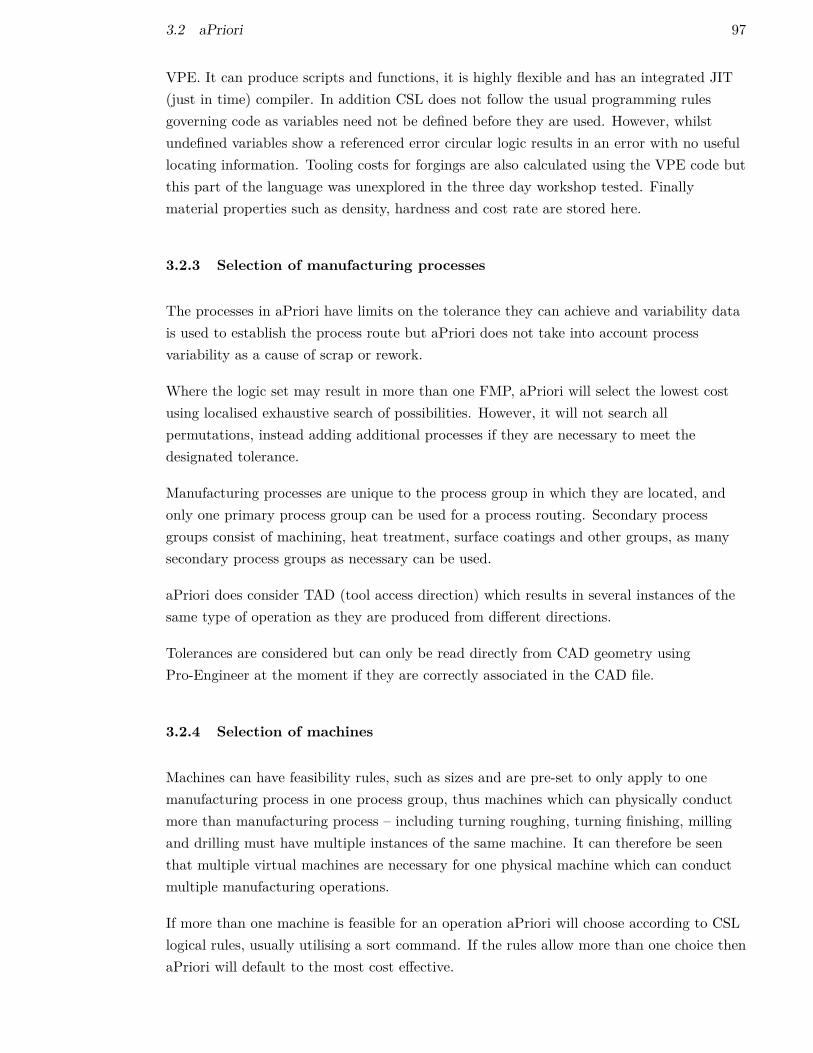
3.2 aPriori 97
VPE. It can produce scripts and functions, it is highly flexible and has an integrated JIT(just in time) compiler. In addition CSL does not follow the usual programming rulesgoverning code as variables need not be defined before they are used. However, whilstundefined variables show a referenced error circular logic results in an error with no usefullocating information. Tooling costs for forgings are also calculated using the VPE code butthis part of the language was unexplored in the three day workshop tested. Finallymaterial properties such as density, hardness and cost rate are stored here.
3.2.3 Selection of manufacturing processes
The processes in aPriori have limits on the tolerance they can achieve and variability datais used to establish the process route but aPriori does not take into account processvariability as a cause of scrap or rework.
Where the logic set may result in more than one FMP, aPriori will select the lowest costusing localised exhaustive search of possibilities. However, it will not search allpermutations, instead adding additional processes if they are necessary to meet thedesignated tolerance.
Manufacturing processes are unique to the process group in which they are located, andonly one primary process group can be used for a process routing. Secondary processgroups consist of machining, heat treatment, surface coatings and other groups, as manysecondary process groups as necessary can be used.
aPriori does consider TAD (tool access direction) which results in several instances of thesame type of operation as they are produced from different directions.
Tolerances are considered but can only be read directly from CAD geometry usingPro-Engineer at the moment if they are correctly associated in the CAD file.
3.2.4 Selection of machines
Machines can have feasibility rules, such as sizes and are pre-set to only apply to onemanufacturing process in one process group, thus machines which can physically conductmore than manufacturing process – including turning roughing, turning finishing, millingand drilling must have multiple instances of the same machine. It can therefore be seenthat multiple virtual machines are necessary for one physical machine which can conductmultiple manufacturing operations.
If more than one machine is feasible for an operation aPriori will choose according to CSLlogical rules, usually utilising a sort command. If the rules allow more than one choice thenaPriori will default to the most cost effective.

98 3 COMMERCIAL COSTING SYSTEMS
Machines have setup times, labour rates, max dimensions etc. They are associated withspecific feature sets and the machine data is both highly detailed and expandable withadditional fields. No programming language experience is necessary to modify these fieldsalthough adding more fields requires use of the in-built programming language.
3.2.5 Cost Modelling
CSL (Cost Scripting Language) is the basis for both the decision on which processes andmachines to use, and the calculation of cycle times and costs. The programming can beadjusted by the user as desired and is compiled at run-time, thus eliminating the problemof slow interpreted code against inflexible compiled code. CSL cannot use or create arrayvariables but this is only an occasional annoyance, and is unlikely to be an insurmountableissue.
Multiple cost categories are available, and each category of costs for each feature iscalculated by code compiled at run-time. Although aPriori does not consider routesequencing explicitly there is an implicit assumption that similar operations are conductedtogether. This was identified by noticing that the incremental cost of similar operations issignificantly lower than the first operation of a specific type. A key category of costs whichis omitted is transport costs, although they could be incorporated within the setup costs.
3.2.6 Assemblies
For assemblies aPriori can calculate the costs of assembly, but the costs of the individualcomponents must be pre-calculated by aPriori, or defined. Assembly; welding, preparationand clean up; and mechanical joins such as riveting can be considered, as can further heator surface treatments. However, aPriori does not automatically have any assemblyautomation. Importing an assembly will automatically result in a short operation to takethe parts and put them on a workbench. Operations such as welding, bolting, or even snapfitting must be added manually as the feature recognition algorithm cannot identify joinsand therefore cannot propose methods of fixing them. In the author’s opinion this is amajor and unnecessary oversight.
3.2.7 Summary of aPriori
The feature recognition capability of aPriori is powerful and it is certainly a substantialimprovement on both other commercial tools and the current approach taken byRolls-Royce internally. However, there are major points for improvement, some of whichare addressed by this research:
3.3 Perfect Costing (Siemens) 99
• There is no uncertainty analysis for design changes; so there is limited and unclearguidance on what to adjust to reduce cost.
• Changing material utilisation does not affect the machining cost, hence it is clearlynot affecting material removal volumes. In addition aPriori will not select the stockshape for the user, instead, rectangular or cylindrical stock must be specified.Allowances for stand-off distance is shown as an option but does not affect the cost,so it is unclear what it is affecting (if anything).
• Output is a set of costs and if necessary a list of the manufacturing methods used butnot the order. This reduces its usability to manufacturing experts because of theirfocus on fixturing and the effect on process rates of part rigidity.
• There are likely to be issues with retrieving data from aPriori if a decision to ceaseusing it were to be taken. The data including costing equations and logic would bedifficult to extract and use, raising the exit cost and potentially resulting in a loss ofbargaining power with the software vendor. The software vendor has assured thatthere is an export facility but this is likely to be just a text dump which will requirefurther work to be useful again alternative models.
• For assembly type operations the joining process must be manually selected, even thefact that there needs to be a joining process must be manually identified.
• In some cases features were found and then quietly ignored as aPriori could notmodel their costs.
Some of the aforementioned shortcomings within aPriori could be overcome with athorough understanding of CSL and modification thereof. Some, however, are intrinsic tothe modus operandi of aPriori and thus more difficult to overcome. It will be demonstratedlater in this thesis that the optimum method of manufacture for a feature depends in parton factors pertaining to other features. aPriori has an deterministic tendency to makerepeated suboptimal decisions, as it does not take a sufficiently holistic view of the designsearch space.
3.3 Perfect Costing (Siemens)
Perfect Costing, available from Siemens has advantages in that it interfaces with theirCAD package (NX) which is the Rolls-Royce corporate geometry modelling tool. However,following a discussion with a Siemens’ representative it was determined that it was in fact aminor improvement on RR CAPP with some tracking and automated recalculation ofprocess times and thus at best no more sophisticated than the aforementioned CFTs(Section 3.1).

100 3 COMMERCIAL COSTING SYSTEMS
Perfect Costing therefore is a simple activity based costing tool with no optimisation, it islimited by the general assumption that the manufacturing route is determined prior to costmodelling and is not affected by it.
The representative from Siemens was unaware of any substantial improvement to PerfectCosting in the near future.
3.4 CATIA
As of 2014 CATIA has had a cost tool integrated within the CAD package (Hiller, 2014),designed for composite components, it allows calculation of the cost of manufacture. Itmust be provided with detailed information on the composite structure, such as plypatterns etc.
3.5 Solidworks costing
Following testing (Figure 3.2) on a very simple hydraulic cylinder and piston it is clear thatthe Solidworks costing tool is fully automated, but fundamentally limited. Solidworksassumed a component machined from a solid rectangular billet and ignored some of thefeatures (Figure 3.3). In addition there was no consideration of tolerances and thus noaccount taken of process variability.
Feature recognition is included to a limited extent, holes are recognised and the programdrew a cuboid around the shape as a representation of the billet to be machined, this wasused to calculate material cost. Unfortunately basic operations such as turning are notused for axisymmetric features and milling appears to not work (the region around thecylinder is un-costed). There is no account taken of tolerances, inspection, failure orrework, order of operations, or the capability of machines. It does run in seconds owing toits simplicity, however it appears to be at best misrepresentative and a placeholder forfurther development.
There are no improvements which the author is aware of planned by Solidworks.
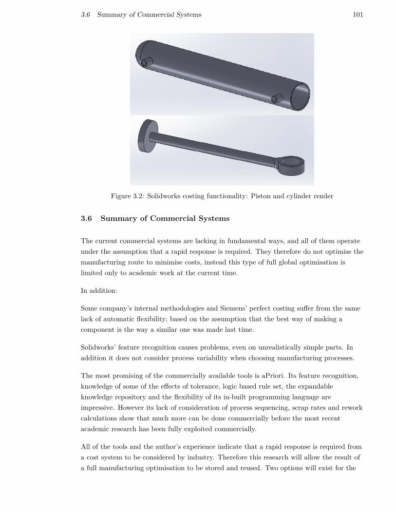
3.6 Summary of Commercial Systems 101
Figure 3.2: Solidworks costing functionality: Piston and cylinder render
3.6 Summary of Commercial Systems
The current commercial systems are lacking in fundamental ways, and all of them operateunder the assumption that a rapid response is required. They therefore do not optimise themanufacturing route to minimise costs, instead this type of full global optimisation islimited only to academic work at the current time.
In addition:
Some company’s internal methodologies and Siemens’ perfect costing suffer from the samelack of automatic flexibility; based on the assumption that the best way of making acomponent is the way a similar one was made last time.
Solidworks’ feature recognition causes problems, even on unrealistically simple parts. Inaddition it does not consider process variability when choosing manufacturing processes.
The most promising of the commercially available tools is aPriori. Its feature recognition,knowledge of some of the effects of tolerance, logic based rule set, the expandableknowledge repository and the flexibility of its in-built programming language areimpressive. However its lack of consideration of process sequencing, scrap rates and reworkcalculations show that much more can be done commercially before the most recentacademic research has been fully exploited commercially.
All of the tools and the author’s experience indicate that a rapid response is required froma cost system to be considered by industry. Therefore this research will allow the result ofa full manufacturing optimisation to be stored and reused. Two options will exist for the

102 3 COMMERCIAL COSTING SYSTEMS
(a) Cylinder cost modelling
(b) Piston cost modelling
Figure 3.3: Solidworks costing functionality

3.6 Summary of Commercial Systems 103
user:
1. A full optimisation will be used to find the optimal method of manufacture when arapid response is not required such as overnight or over a weekend, with the optimummanufacturing route being stored.
2. A real time response option which reuses the stored manufacturing route in (1) andrecalculates costs for new geometry or changes in tolerance.
Approach (2) would compete with commercial systems to give a real time response but thedependency on (1) would require regular reruns of (1) thus keeping the baseline up to datewith design changes.
This research will not have feature recognition functionality which is desirable from acommercial and usability perspective. It is therefore thought that future work could be tointegrate this with feature recognition which would create a product superior in all ways tocurrent commercial tools.

104 3 COMMERCIAL COSTING SYSTEMS

105
4 FoSCo (Forming Shape Creator)
The overall system presented in this research attempted to deduce the optimal method ofmanufacture, and the cost thereof, given the finished part geometry. This methodology, tobe executed in a computer or similar device, is submitted for patent in the USA and theEU.
EU patent number 16180366.3 - 1954
US patent submission reference 5895 LMT
Contained within Section 8 is the full patent application for FoSCo.
This research, in accordance with industry practice, assumed a constant specific cost of theselected material, and calculated the shape which can be created during the primaryforming process or manufacturing strategy.
The purpose of FoSCo is to allow the design feature file to contain the exact amount ofmaterial ‘removed’ during the forming process, thus making possible the accuracy of theManufacturing Choice Optimisation and Sequencing Tool (MCOST). This virtual removalsaves on material cost, although it may increase the cost of the mould or process, due toincreased complexity or increased forging time. Awareness of the extent of materialremoval required after the forming process allows the calculation of times, and thus costs,of later material removal processes.
Thus the objective of FoSCo is to identify the shape which would be made by a formingprocess, from this the depth of cut required to machine away the excess material (if any),can be calculated. The distances, between the Final Machined Part (FMP) geometry andthe formed shape, are then used by MCOST which requires material removal volumes tocalculate machining time.
As discussed in Section 2.4, there has been research to determine the geometry which willbe created by forging operations. However, this section will present a new method, amethod which does not require an extensive rule set to operate. Two approaches were usedin this research: face or edge offset for near-net-shape manufacturing strategies, and themethodology to be described where the manufacturing strategy creates smooth shapesaround the FMP.
The approach was intended to be modular thus enabling different codes or modules to beused for different component types, or forming methods, and is thus expandable. Becauseof the nature of the co-ordinate system used by the default FoSCo convergence module, thesmoothing algorithm is unsuitable for some types of shape, and for some types of formingprocess (particularly near net shape methods and shapes with multiple concave surfaces).Methods to resolve this are to be presented in future work. It should be noted however,

106 4 FOSCO (FORMING SHAPE CREATOR)
that whilst this method may not calculate the exact forming shape in all cases, it has notyet failed to find an estimate of the forming shape, which more complex rules basedmethods can. It will thus give an indication of whether a design change will result in apositive or negative change in cost, and an approximate magnitude even if the absolutevalue is inaccurate3.
The two 2d test cases, and their predicted forming shapes, are shown in Section 4.4.12. Forthe blisk test case there is also:
• The industrial sponsor’s manual estimate of the forging shape.
• The estimate of the forging shape from the industrial sponsor’s proprietary forgingshape creator tool (ACE).
• The finished part axis-symmetric profile.
The 3d version of FoSCo used for test case two (the engine section stator) is intended as anillustration of the flexibility of the methodology presented (Section 4.5.5).
4.1 Precursor Technologies
It is assumed that the manufacture of the test cases (Sections 1.8), involves creating ashape which is everywhere larger than or equal to the finished part geometry (FPG). Thisshape is referred to as the precursor or forming shape, and is created by a primary formingprocess. It is apparent that for manufacturing it may sometimes occur, that componentsare made by joining additional material, usually by welding. However, when this occurs itis proposed that the additional sections are analysed separately, and analysis is conductedfor the assembly process. The cost of the assembly process is out of the scope of this thesis,and is outlined for incorporation in future work (Section 6.5.3).
Given that in some primary forming processes additional material will be present (inaddition to the FPG). The extraneous material is then removed until the FPG is achieved.For a net shape manufacturing strategy, this material removal will be zero; for near netshape, minimal; and for legacy manufacturing strategies, potentially large such as 12:1(Blose et al., 2006). Additive technologies could be considered net shape primaryshaping processes, and therefore be modelled by this methodology.
However additive technologies have been defined as out of scope for FoSCo, this is because:
1. The additive technology may impose additional requirements intrinsic to the processsuch as: printed support structures, or powder removal passages. A dedicated tool isthought superior for these technologies.
3George Box (1978) - All models are wrong but some are useful

4.1 Precursor Technologies 107
2. The use of additive technologies often enables substantially different geometric designto maximise the benefits. In other words, if a component is to be produced throughadditive manufacture, it is likely to be too dissimilar to allow direct comparison withtraditional manufacturing.
For test cases zero, one and two, at least two different primary forming processes will beconsidered.
The methodology behind the generation of these shapes is essentially a smoothingalgorithm, derived from an iterative implementation of image recognition algorithms Kasset al. (1988). It was modified to a polar co-ordinate system for a closed contour and togive a stand-off distance.
It essentially has three stages:
1. Export of FMP (Finished Machined Part) data from NX, either as a two dimensionalset of lines or a three dimensional surface mesh. It does not at present operate withcurves or splines but this would be a simple and obvious improvement.
2. Calculation of a closed loop of points (2d), or a point surface (3d), which representsthe forming shape.
3. Import of this ring/surface into NX and calculation of the distances between theFMP and the forming shape.
These tasks could all be completed within the NX API but for ease of debugging they werekept outside for the prototype software.

108 4 FOSCO (FORMING SHAPE CREATOR)
4.2 Nomenclature
Acronyms
Acronym Meaning
FMP Final Machined PartFMPP FMP Point: A point on the surface of the final machined partFSP Forming Shape Point: A point on the surface of the forming/precursor shape
MCOST Manufacturing Choice Optimisation and Sequencing ToolPOI The Point Of Interest, defined as the FSP currently being examined
Variables
Symbol Meaning
B The vector from the closest FMPP to the POI.B̂ The unit vector of BCP The location of the convergence point (specific to one or more FSPs)D The vector between the FSP and the closest FMPPfd Damping factorL The Cartesian co-ordinates of the POIm Magnitude of movement of the POIM The total movement applied to the FSP before time step control and dampingMP The closest final shape point (FMPP).M1 A constant movement vector towards CP
M2 A constant movement vector towards the closest FMPPM3 An inverse square movement vector away from the closest FMPPn The vector from the POI to the Convergence Point to which it is assignedn̂ The unit vector of nNP The Cartesian co-ordinates of the closest FMPPr The radius of the POIx Minimum euclidean distance between adjacent FSPs
Co-efficients (numerical value specific to each forming technology)
Co-efficient Meaning (Specific to each manufacturing technology)
k1 The co-efficient which controls the magnitude of M1
k2 The co-efficient which controls the magnitude of M2
k3 The co-efficient which controls the magnitude of M3
k4 The co-efficient which controls the magnitude of the curvaturesmoothing correction

4.3 FoSCo Architecture 109
4.3 FoSCo Architecture
The architecture for FoSCo is shown in Figure 4.1. It can be seen that the basicarchitecture of both the 2d and 3d versions is the same, the only differences between themare in the method of import of the FMP geometry, and the simplified equations for the 2dversion (due to the z co-ordinate being always zero, and only two adjacent points forsmoothing).
Figure 4.1: FoSCo architecture
For both the 2d and 3d versions of FoSCo the secondary convergence (Section 4.4.8) usesan energy balance type equation, with a movement vector force pulling the Forming ShapePoint (FSP) towards the nearest Final Machined Part Point (FMPP) and an inversesquared movement vector pushing it away. A centre convergence movement vector is alsoused to move points towards the centre when their closest point is perpendicular to theirunit vector towards the origin. An excessive convergence filter within secondaryconvergence is also used, and described later.
Tertiary convergence is a smoothness correction necessary for the shape generation,described for FoSCo 2d in Section 4.4.9. This algorithm was not implemented in FoSCo 3dand this is left as future work.
An algorithm for primary convergence is also described, it has no effect on the final resultbut it reduces the number of iterations required in secondary convergence, thereforereducing the time taken to evaluate the forming shape. It was implemented for both 2dand 3d versions of FoSCo.

110 4 FOSCO (FORMING SHAPE CREATOR)
Both versions also use adaptive grid spacing, to provide adequate definition of the shapegenerated without excessive computation.
Clearly for the two dimensional version the z co-ordinate is always zero, simplifying thecalculations, in addition there are only two adjacent points in the 2d version, simplifyingthe smoothness correction.
4.4 FoSCo methodology (2d) 111
4.4 FoSCo methodology (2d)
Creation of the forming shape is a multiple step process involving primary convergence,secondary convergence, and a smoothing algorithm. The primary convergence is a lowoverhead initial phase, to reduce the solution time. The secondary phase is a balancebetween convergence forces and inverse squared repulsion from the closest FMPP (FinalMachined Part Point). The smoothing algorithm will increase the radius of points whichare too far out of alignment with their neighbours. In addition to the above algorithms,there is adaptive grid spacing to ensure an even distribution of points. The stored data oneach point are: its angle (theta); its radius (r); and whether it is deemed to have stopped.Theta is fixed for each point, but the radius varies.
The step by step explanation of the methodology begins in Section 4.4.5, with themethodology importing a set of lines which form a closed contour from CAD geometry.Prior to this some supporting functions should be explained, namely the co-ordinatesystem, convergence points, adaptive grid spacing, and finding the appropriate FMPP fromthe set.
4.4.1 Co-ordinate Systems
One of the hardest questions to answer when attempting to generate forming shapes is howto define a co-ordinate system, in particular the consideration of neighbours. A Cartesiansystem of points can specify any point in n dimensions, but has no implicit concept ofneighbours, a radial/spherical co-ordinate system on the other hand can use the angle(s) todefine neighbours. It can easily be seen that neighbours are essential to predicting theshape to be generated by a forming process, as to suggest that a point on a relativelysmooth surface can be unaffected by the position of adjacent points is axiomatically false.
So, given that a closed contour or surface must clearly be formed, either by designating aset of points, or an equation which can be solved. Given also that the placement of aparticular point on the surface (representing the surface of a formed shape) is dependanton several factors including the position of adjacent points, some method of definingadjacent points and preferably keeping the same neighbours throughout the algorithm isnecessary. The method presented here is the use of a combination of the Cartesian andpolar co-ordinate systems, where adjacency can be defined using the theta value in polarco-ordinates, but placement calculations can be conducted after a polar to Cartesianco-ordinate transformation. One of the issues with the use of a polar co-ordinate system isthat of shading, certain regions of space become shaded (Figure 4.2). On the first graph,Figure 4.2a, some regions are inaccessible by a shrinking circle without first passingthrough the finished part geometry, and the methodology fundamentally prohibits this. Forsimple shapes this issue [shading] can be alleviated with careful placement of the shaperelative to the origin (Figure 4.2b) of the polar co-ordinate system.

112 4 FOSCO (FORMING SHAPE CREATOR)
For more complex shapes it can become impossible to locate the origin such that shading isnot an issue somewhere. Hence the creation of the convergence line, a concept wherebyadjacent forming shape points may use a similar co-ordinate system, but with a differentorigin in Cartesian space. Or to put it another way, there are multiple polar co-ordinatesystems contained within the Cartesian space. This concept means that areas consideredshaded and thus inaccessible for one FSP and its co-ordinate system are accessible toothers. An algorithmic method of determining the convergence point is now required,described in Section 4.4.2.
(a) Origin in original position, casting shape clearly un-representative
(b) Origin moved to reduce shading of casting process
Figure 4.2: The issue of shading when a point is used for convergence (Test case two geom-etry)
4.4.2 Finding the convergence point
One of the important aspects of this algorithm is that the FSPs do not all converge to thesame point (that is if the radius of all the FSPs were zero, a line would be formed). It isthis aspect of the algorithm which allows the shape created to be close to the FMP shapein a near net shape manufacturing process. The convergence line is at present manuallydefined and should be enveloped by the FMP shape, the end points of the line should notbe too close to each other relative to the origin (0,0) of the native co-ordinate system. Thisis because when the convergence line is constructed the end points are assigned a range ofangles, based on the line from the origin to the end point ± 15º, as shown in Figure 4.5,within which all FSPs are assigned to them [the end points]. Ergo if the start and endpoints are too close to each other in theta value relative to the native co-ordinate system,these 15 degree triangles could overlap. The convergence line defined has start and endpoints with angles from the positive x-axis in the anti-clockwise direction of λ and φrespectively.
For each FSP (Forming Shape Point), a convergence point is defined. Which convergencepoint is used is dependant only on the θ value assigned to that point (which does not vary).

4.4 FoSCo methodology (2d) 113
It can thus be seen that from the moment an FSP is defined, its θ value is defined andconstant, and thus its convergence point is also defined and constant. FSPs which do notfall in the range of λ± 15º or φ± 15º (the range of θ angles applicable to the start or endpoints respectively) are assigned one of the intermediate convergence points in accordancewith Algorithm 1.
Algorithm 1 is used, and the mapping for an example convergence line (Figure 4.3) can beseen in Figure 4.4a Figure 4.4b. Essentially whilst θ = λ± 15º we are held at index zero, aswe traverse the angular space between the upper bound of λ± 15 and the lower bound ofφ± 15 we move up through the indices of the convergence line, whilst θ = φ± 15º we areheld at the maximum index of the convergence line, then as we continue on aroundincreasing θ we return back down the indices.
This angle (15º) is detemined by the fact that some FSPs should be present within its arc,thus the angle is determined by the interaction of the stand off distance of themnufacturing process, the distance from the end of the convergence line to the FMP shape,and the spacing of the FSPs. It is left to future work to derive this angle automatically,but tests did not show a significant deterioration of the algorithm performance when theangle was changed to 10º or 20º.
Figure 4.3: The convergence line with start and end points shown

114 4 FOSCO (FORMING SHAPE CREATOR)
(a) The convergence line with an intermediate set ofFSPs (lines connect the FSP with its convergence point
(b) A magnified graph of Figure 4.4a
Figure 4.4: FSPs linked to their convergence points
Figure 4.5: Graph showing the range of theta values within which FSPs belong to theconvergence point at the end of the convergence line

4.4 FoSCo methodology (2d) 115
Algorithm 1 Finding the index of the convergence point applicable to this POIMin = 0.5, i.e. the smallest number which (when rounded) will refer to the second point onthe convergence line.Max = Number of points on convergence line - 1.5000000001, i.e. the largest number which(when rounded) will refer to the penultimate point on the convergence line.Difference = Max - Min
if (θ is between λ - 15º and λ+ 15º) // Use FUNCTION IsAngleBetweenIndex = 0
else if (θ is between φ - 15º and φ + 15º)Index = Last index of Convergence Line
else if (θ is between λ+ 15º and φ - 15º))NonDimDistanceAround = GetNonDimensionalDistanceAroundAnArc((φ− 15º) −
(λ+ 15º), θ, λ+ 15º)Index = Round to integer (NonDimDistanceAround * Difference + Min)
else if (θ is between φ+ 15º and λ− 15º))NonDimDistanceAround = GetNonDimensionalDistanceAroundAnArc((φ+ 15º) −
(λ− 15º), θ, φ + 15º)Index = Round to integer (Max - NonDimDistanceAround * Difference)
WHEREFUNCTION GetNonDimensionalDistanceAroundAnArc(ArcLength, Theta, ArcStart)
if (θ < ArcStart)Add 2π to θ
return (Theta - ArcStart) / ArcLength
FUNCTION IsAngleBetween(Angle, LowerBound, UpperBound)if (LowerBound > UpperBound)
LowerBound -= 2 * Math.PIif (Angle >= LowerBound AND Angle <= UpperBound)
return trueelse
Angle -= 2 * Math.PIif (Angle >= LowerBound && Angle <= UpperBound)
return truereturn false
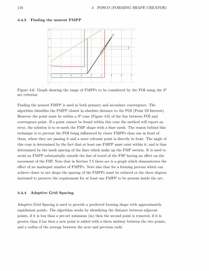
116 4 FOSCO (FORMING SHAPE CREATOR)
4.4.3 Finding the nearest FMPP
Figure 4.6: Graph showing the range of FMPPs to be considered by the POI using the 3ºarc criterion
Finding the nearest FMPP is used in both primary and secondary convergence. Thealgorithm identifies the FMPP closest in absolute distance to the POI (Point Of Interest).However the point must be within a 3º cone (Figure 4.6) of the line between POI andconvergence point. If a point cannot be found within this cone the method will report anerror, the solution is to re-mesh the FMP shape with a finer mesh. The reason behind thistechnique is to prevent the POI being influenced by closer FMPPs than one in front ofthem, where they are passing it and a more relevant point is directly in front. The angle ofthis cone is determined by the fact that at least one FMPP must exist within it, and is thusdetermined by the mesh spacing of the lines which make up the FMP section. It is used toavoid an FMPP substantially outside the line of travel of the FSP having an effect on themovement of the FSP. Note that in Section 7.5 there are is a graph which demonstrates theeffect of an inadequet number of FMPPs. Note also that for a forming process which canachieve closer to net shape the spacing of the FMPPs must be reduced or the three degreesincreased to preserve the requirement for at least one FMPP to be present inside the arc.
4.4.4 Adaptive Grid Spacing
Adaptive Grid Spacing is used to provide a predicted forming shape with approximatelyequidistant points. The algorithm works by identifying the distance between adjacentpoints, if it is less than a pre-set minimum (m) then the second point is removed, if it isgreater than 2.1m then a new point is added with a theta midway between the two points,and a radius of the average between the next and previous radii.
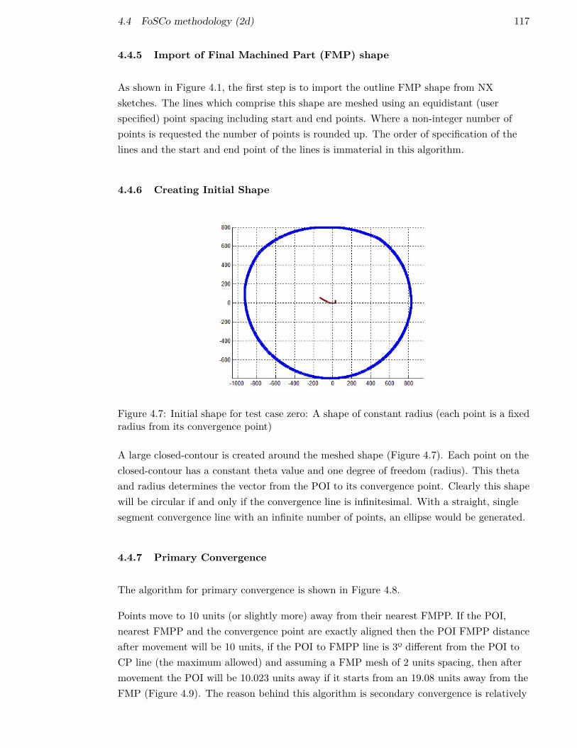
4.4 FoSCo methodology (2d) 117
4.4.5 Import of Final Machined Part (FMP) shape
As shown in Figure 4.1, the first step is to import the outline FMP shape from NXsketches. The lines which comprise this shape are meshed using an equidistant (userspecified) point spacing including start and end points. Where a non-integer number ofpoints is requested the number of points is rounded up. The order of specification of thelines and the start and end point of the lines is immaterial in this algorithm.
4.4.6 Creating Initial Shape
Figure 4.7: Initial shape for test case zero: A shape of constant radius (each point is a fixedradius from its convergence point)
A large closed-contour is created around the meshed shape (Figure 4.7). Each point on theclosed-contour has a constant theta value and one degree of freedom (radius). This thetaand radius determines the vector from the POI to its convergence point. Clearly this shapewill be circular if and only if the convergence line is infinitesimal. With a straight, singlesegment convergence line with an infinite number of points, an ellipse would be generated.
4.4.7 Primary Convergence
The algorithm for primary convergence is shown in Figure 4.8.
Points move to 10 units (or slightly more) away from their nearest FMPP. If the POI,nearest FMPP and the convergence point are exactly aligned then the POI FMPP distanceafter movement will be 10 units, if the POI to FMPP line is 3º different from the POI toCP line (the maximum allowed) and assuming a FMP mesh of 2 units spacing, then aftermovement the POI will be 10.023 units away if it starts from an 19.08 units away from theFMP (Figure 4.9). The reason behind this algorithm is secondary convergence is relatively

118 4 FOSCO (FORMING SHAPE CREATOR)
Figure 4.8: Primary Convergence Algorithm
Figure 4.9: Movement of one POI where FPG mesh is two unit spacing and Cp is at (0,0)
slow and computationally expensive, this algorithm reduces the distance secondaryconvergence must cover, thus reducing time taken. The end result for primary convergenceis shown in Figure 4.10. As can be seen the shape is now much closer to the finished partgeometry, giving much less distance for the secondary convergence algorithm to cover.
The reasoning behind the ten unit value is, forging for the type of components modelledwould be expected to leave a stand off distance of six units. The number of 10 unitstherefore results in bringing the POIs close to the FPG but not so close that they wouldimmediately move away. It would be feasible to set the value to exactly the stand offdistance for the manufacturing method thus minimising secondary convergence time, butthis would not change the end result.

4.4 FoSCo methodology (2d) 119
Figure 4.10: After the primary convergence algorithm, test case zero

120 4 FOSCO (FORMING SHAPE CREATOR)
4.4.8 Secondary Convergence (for n2 iterations)
Figure 4.11: Secondary Convergence Algorithm
The points are drawn along their line of freedom according to: A force pulling them towardstheir convergence point (F1) A force pulling them towards the nearest FMPP (F2) A forcepushing them away from the FMPP (F3) So the red points (FSPs) are pulled in wherefurther away from the blue points (FMPPs) and pushed out where closer to the FMPPs.
Movement governed by following equations:
Definitions:
CP =
xc
yc
0
(4.1)
L = cp + r
sin (θ)cos (θ)
0
(4.2)
n = r
sin (θ)cos (θ)
0
(4.3)
n̂ = n
|n|(4.4)
B = L−Mp (4.5)
B̂ = B
|B|(4.6)

4.4 FoSCo methodology (2d) 121
Forces
F1 = k1 · n̂ (4.7)
F2 = k2 · B̂ (4.8)
F3 = k3 ·B̂
|B|2(4.9)
F =3∑
n=1Fn (4.10)
m = F · n̂ (4.11)
Important points:
The Equations for the forces are shown above; the coefficients are tuned to themanufacturing process.
F1 is a constant force pulling the Forming points towards the convergence point.
F2 is a constant force pulling them towards the closest FMPP.
F3 is an inverse squared force pushing away from the closest FMPP.
Different values of k1, k2, k3 are used for different types of forming process (example valuesin Table 4.1). These values were found by trial and improvment. By increasing all valuesby the same factor, the end result should be unchanged and arrived at sooner, however, itwas found that a high k3 value will tend to result in numerical instability in what iseffectively euler integration.
In Section 7.5, graphs are shown giving an example of the directions and magnitude of F1,F2, F3, and the resultant movement vector. These graphs show that when the FSP is atpoint (8,8) there is still a net force moving it inwards, by the time it has moved to (7,7) theresultant force is outwards. This implies that the point will come to rest somewherebetween (8,8) and (7,7). Note that these graphs show that in this case the convergencepoint is at (0,0), there is only one FMPP within the three degree arc described in Section4.4.3, and this is located at (3,3).
Saturation limits are placed to reduce movement where it exceeds a value x. Where x isreduced linearly to zero at the end of secondary convergence. The reasoning behind thesewas a tendancy in some cases for the equations to result in dynamic instability and anoscillating divergence.

122 4 FOSCO (FORMING SHAPE CREATOR)
Casting Die Forging Roll ForgingSecondary Convergence k1 1 1 1Secondary Convergence k2 1 1 1Secondary Convergence k3 -5 -50 -50Tertiary Convergence r 0.1 0.005 0.005
Table 4.1: Convergence co-efficients - Example values of k and r used
4.4.9 Smoothing (Tertiary Convergence)
This is executed iteratively until all points exhibit no more movement or until a userdefined iteration limit is reached.
Figure 4.12: Tertiary Convergence Algorithm
Where a point is too far inside a line traced between the previous and next points, theradius is increased to meet the requirement.
As shown in Figure 4.13. This is done by finding the vector between the points either sideof the POI, drawing a line (A) between them, calculating the shortest vector (B) betweenthe POI and A. The allowable magnitude of B is defined as r|A| where r is a value definedby the forming process (example values in Table 4.1). If |B| > the allowable magnitudethen the point is moved out along its position vector until it no longer exceeds theallowable magnitude (Algorithm 2). Clearly moving a point out may mean neither, one orboth adjacent points now deviate by more than the allowable amount, so the algorithmrepeats until no points deviate excessively. The end result of tertiary convergence is shownin Figure 4.14. The process is of course iterative because as one point moves out, itsneighbours then become too far in. The method used, simply repeating this process is lessefficient than possible, more efficient ways of knowing which points might need to move(i.e. the neighbours of moved points) could be implemented, but this would have no effecton the final solution.

4.4 FoSCo methodology (2d) 123
Figure 4.13: Teritary convergence - previous, current and next and vectors
Figure 4.14: Test case two - end of tertiary convergence

124 4 FOSCO (FORMING SHAPE CREATOR)
Algorithm 2 The tertiary convergence algorithmFor all POI
if (DotProduct(B, UnitVectorToConvPoint) < 0) // if point is inside VectorNextPrevi-ous
if (|B| > r / |A|)Successful = false; // When no points move in the iteration, tertiary conver-
gence will terminate.Movement = |B| - (r / |A|) * 0.999 // This value will always be positive.Increase the radius of POI byMovement // A positive value will increase radius
of the POI by ’Movement’

4.4 FoSCo methodology (2d) 125
4.4.10 Fixed points
In FoSCo2d, there is the option to fix edges of the forming shape. This is to allow forconstraints such as in blisks where the centre is not hollow, not a fundamental requirementof forging but required by strain rate restrictions and cost reasons. Rules such as this couldbe included within a rule based method.
At the present, it is allowed for by specifying an angular range and a fixed x or ydisplacement. It allows for effects such as shown in Figure 4.20. In this example, pointswith a theta of 270 degrees ±3 are specified to lie n mm below the absolute origin of themodel within the geometry creation CAD package. This corresponds to the location of theaxis around which the shape is revolved. Three degrees was used to give the appropriatewidth of material at n mm below the origin of the CAD package. This angular range anddisplacement for fixed lines could be deduced from data read from the CAD package infuture through the use of appropriately named lines or a .dlx based solution.
This capability was used to generate the disk forging shape shown in Figure 4.19.
4.4.11 Import of created shape into CAD package
The forming shapes are imported back into NX as new sketches, the 2d version is importedas a ring of points onto the same plane as the sketch from which the main shape isrevolved).
To analyse the depth of material removal required, the start and end points of eachrelevant line in the model are analysed to find the closest point in a direction perpendicularto the type of line (i.e. it is defined as a left, right, top or bottom line). A referencedimension is then created in the appropriate direction for later export from NX. Thesereference dimensions can be used in the interface spreadsheet between NX and MCOST inthe knowledge they will be regenerated with the same names when the part is modified.Dimensions are created automatically according to the systematic naming convention:“COS2” + “END” OR “START” + Name(Line).
4.4.12 FoSCo 2d Results
The graphs below (Figure 4.16, Figure 4.17) show plots FoSCo 2d on test cases zero andone. It can be seen that the convergence of casting for test case zero is imperfect, this isdue to the nature of the algorithm for finding the convergence point, and could be rectifiedby using adaptive grid spacing for the convergence line. On test case zero there is alsosome stagger in the points around the edge of the flange, caused by a mismatch ofconvergence points, i.e. in radial co-ordinates they are not adjacent. This is caused by

126 4 FOSCO (FORMING SHAPE CREATOR)
Figure 4.15: Diagram of the 2d imported point ring plus automatically created referencedimensions
primary convergence causing an irrevocable convergence, however it does not affect thevalidity of the shape from a cost point of view.
Adjustment of the FPG (Finished Part Geometry) Changing the FPG and theadjustments that FoSCo will make to the forming shape are shown in Figure 4.18.
In this way, by running FoSCo and MCOST after design changes have been made, theeffect on the cost can be rapidly evaluated, as of course the changes will affect themachining depths and thus times and costs of the manufacturing operations.
FoSCo was also run for blisk geometry, the resultant shape (Figure 4.19) is generated for ablisk. The co-efficients used for the k values and smoothing algorithm were identical tothose used for ring roll forging for test cases zero and one, suggesting the flexible validity ofthe method. The only requirement was to set fixed points to account for a roll forging (nothollow) as opposed to a ring roll forging (hollow).
4.4.13 Calibration and testing
FoSCo 2d was calibrated against expert estimation of the die forging shape for a rear outercasing. It was then tested against a blisk (using the same kn co-efficients) Table 4.2. Thethree images in Figure 4.20 show: the finished part geometry, an expert’s estimation of thedie forging shape (although the expert provided a rectilinear estimate rather than thecurved shapes normally associated with die forging), FoSCo’s estimate of the die forgingshape. To use FoSCo for die forging it was also necessary to incorporate a method ofpreventing hollow shapes as these are not created using die forging, this was implementedby fixing some of the points (in the ring of points) at a specified radius. This fixing was

4.4 FoSCo methodology (2d) 127
Figure 4.16: Test Case Zero, Simplified RoC (Rear Outer Casing) and its forming shape plot
completed manually through code but the requirement to fix the central section at nonzero thickness is not a fundamental constraint requirement of die forging. The industrialsponsor’s die forged shapes do not have zero thickness due to cost reasons and structuralconsequences of the strain rate required to achieve zero thickness.
Description Type Volume (dm^3)Finished Part Geometry FPG 8.68
FoSCo estimate (co-efficients as for ring roll forging) Black Forging 21.39Sponsor’s Estimate (manual) Black Forging 22.13 (+3.3%)
Sposor’s Estimate from rules based tool (ACE) Black Forging 23.27 (+8.08%)
Table 4.2: FoSCo’s estimate of forging volume against professional estimate from industrialsponsor

128 4 FOSCO (FORMING SHAPE CREATOR)
Figure 4.17: Test Case One, RoC (Rear Outer Casing) and its forming shape plot
(a) Original shape (b) Increased flange height
(c) Reduced flange thickness (d) Reduced casing angle
Figure 4.18: Design changes and their effect on the formed shape (of Test Case Zero)

4.4 FoSCo methodology (2d) 129
Figure 4.19: FoSCo 2d with a blisk input as finished part geometry, governing co-efficientsas set for test case zero and one

130 4 FOSCO (FORMING SHAPE CREATOR)
(a) Axis-symmetric finished part geome-try
(b) Forging Shape -estimated by industrialsponsor using ACE(rules based tool)
(c) Forging Shape - estimated by industrialsponsor (ignoring fillets)
(d) Forging shape - estimated by FoSCo
Figure 4.20: Blisk FoSCo 2d testing
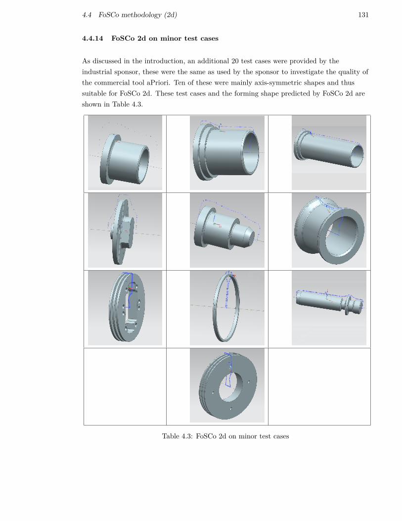
4.4 FoSCo methodology (2d) 131
4.4.14 FoSCo 2d on minor test cases
As discussed in the introduction, an additional 20 test cases were provided by theindustrial sponsor, these were the same as used by the sponsor to investigate the quality ofthe commercial tool aPriori. Ten of these were mainly axis-symmetric shapes and thussuitable for FoSCo 2d. These test cases and the forming shape predicted by FoSCo 2d areshown in Table 4.3.
Table 4.3: FoSCo 2d on minor test cases

132 4 FOSCO (FORMING SHAPE CREATOR)
4.5 FoSCo methodology (3d)
The 3d version of FoSCo is less developed than the 2d version, simple further work isoutlined and is left as further work. Plots of the overall methodology are shown in Figure4.21. Finding the closest FMPP is not restricted to Cartesian distance without anyconsideration of angle as in Section 4.4.3.
(a) Create a sphere (b) Primary Convergence: Move 90%of distance towards nearest point
(c) Secondary convergence: based onrules and equations above
(d) Finished
Figure 4.21: Stages of FoSCo 3d convergence
4.5.1 Initial shape
The 3d version is similar to the 2d version except that the 3d version starts with a sphereof points created from multiple circles. The nature of the co-ordinate conversion usedcreates the effect shown in Figure 4.22. FoSCo3d at present uses only a convergence point,rather than a line, polygon or polyhedron. This could potentially be future work toimprove convergence.
1. Parallelise for all forming methods to be considered.
(a) For n iterations
i. The points are drawn along their line of freedom according to:
A. A force pulling them towards the originB. A force pulling them towards the nearest mesh point

4.5 FoSCo methodology (3d) 133
Figure 4.22: The initial placement of points (example shows 7 circles, 400 points per circle)
C. A force pushing them away from the mesh point
ii. Their movement is then calculated and the iteration is complete.
(b) The creator is complete when a set number of iterations have occurred.
As shown in Figure 4.1, initially a mesh is imported directly from an NX surface meshexport.
The methodology then divides into parallel threads, one for each manufacturing strategy.The surface of a sphere is created around the meshed shape where each point on surfacehas a radius of the radius of the furthest point on the FMP plus 10mm.
The convergence towards the forming shape then consists of primary and secondaryconvergence phases, with differing governing equations. During convergence the points areallowed to vary only in radius and the user specifies the number of iterations in theprimary and secondary phases. Adaptive grid spacing is used in the 3d version, but onlybetween points on the same circle (points of constant ϕ). Changing this to consider spacingbetween adjacent circles is left to further work.
4.5.2 Primary convergence
For primary convergence the points are moved inwards 90% of their distance to the nearestFMPP. This is simply to bring the circle of points closer to the FMP to minimise thenumber of iterations required in the secondary phase. The algorithm used is the same as a

134 4 FOSCO (FORMING SHAPE CREATOR)
previous version of the algorithm used in Section 4.4.7. In the 2d version it was replacedwith an algorithm to move the point to approximately 10 units away, which is morecomputationally efficient.
4.5.3 Secondary convergence
For secondary convergence the movement value of each point is calculated using Equation4.12. During secondary convergence adaptive grid spacing is used as in the 2d version(Section 4.4.4).
The equation which defines the movement of the point during secondary convergence is:
m = (M · n̂) ts (1− fd) (4.12)
M =3∑
n=1Mn (4.13)
M1 = k1n̂
M2 = k2D̂
M3 = k3D̂/d2
(4.14)
D̂ = L−NP
|L−NP |(4.15)
n̂ =
− cos (θ) cos (φ)− sin (θ) cos (φ)− sin (φ)
L = r
cos (θ) cos (φ)sin (θ) cos (φ)
sin (φ)
(4.16)
It can be seen that the equations for the 2d version are the same equations (in 2d φ isalways zero, so z is zero).
As with the 2d version the 3d version also has checks to ensure smoothness and to checkthat the point ring does not violate the finished part geometry. However, whereas the 2dversion has a separate algorithm for smoothness implemented after secondary convergence,in the 3d version smoothing is at present located within secondary convergence.
For smoothness

4.5 FoSCo methodology (3d) 135
If (AverageRad > ThetaRadContinue.Item2[i0] - Movement + Forces[3])
Movement = -(AverageRad - Forces[3] - ThetaRadContinue.Item2[i0]);//Movement = -0.5;
This means that if the average radius of the radii of the two adjacent FSPs exceedsthe (after movement) radius of the FSP under consideration plus an allowed amountof divergence, the movement is reset to -0.5. This creates a small outward movement.The lower Forces[3] is set the smoother the shape will be.
Despite the 3d nature of the sphere representing the FSPs there is no interactionbetween adjacent circles making up the sphere, this is left as further work. Toaccomplish this is a minor extension of the work to identify which of the points onadjacent circles is closest since not all circles have the same number of points on them.
For excessive convergence
if (Abs(Movement) > Forces[0] + Forces[1] + 1) // too much movement, point isprobably within FMS (and thus being pushed inwards by M3.
Movement = -1;
This is effectively a saturation monitor. If the movement is too great either inwardsor outwards then the movement is set to -1, a small outward movement, themovement will normally be too great after the FSP violates the FMP since there willbe no balancing force after violation.
4.5.4 Output and NX import
The final shape of the point surface is then exported to a .txt file which is used by codewritten in NX to import the point cloud as a 3d surface (graphics can be enabled or not)to which is used to analyse the depth of material removal required:
1. A 3x3 grid is placed over each surface in the component
2. The normal direction at the centre of the surface and its location relative to the NXorigin (used as a proxy for centre of gravity in the test case) are analysed to give anindication of the machining direction.
3. The closest forming point in the appropriate direction (see 2) is found, and thedistance in that direction is stored for the 3x3 grid. The average is calculated fromthe points to give an average depth of cut for that face. The average is unweightedbecause the algorithm which constructs the 3x3 grid provides points where the areaclosest to each point is approximately equal.

136 4 FOSCO (FORMING SHAPE CREATOR)
Figure 4.23: Diagram of the face surface grid created
4.5.5 Results of 3d FoSCo
The results of FoSCo 3d for test case two (4.25) for several forming processes are shown inFigure 4.26.
The result of FoSCo 3D for ARCAM and casting (Figure 4.26) is clearly inaccurate for anear net shape process. However, where supporting structure is required this couldpotentially be modelled using the approach used in FoSCo 2d (Section 4.4.10 FixedPoints). To model the contours of a net shape accurately however the two dimensionalapproach of a convergence line must be expanded, to allow a polygon in three dimensionalspace. This was not explored in detail but alluded to in the future work section. This lackof accuracy for near net shape processes is the cause of overestimation of the cost of testcase two by MCOST (Section 5.12.4).

4.5 FoSCo methodology (3d) 137
Figure 4.24: Point cloud imported into NX
Figure 4.25: Test Case Two, ESS (Engine Section Stator) and its forging shape plot
(a) Die Forging (b) Casting (c) ARCAM
Figure 4.26: FoSCo 3d results for ESS

138 4 FOSCO (FORMING SHAPE CREATOR)
4.6 Alternative modelling methods
Alternative methods were considered, a rules based method was considered unattractivedue to the time required to populate the rules for the specified component to be examined.Alternative simple methods were an offset method, where lines are simply offset a specifieddistance x, and a rolling circle method proposed by Toal (2012) where a circle traces aline around a shape and the centre of the circle delineates the forming shape. These wereconsidered and found to be inadequate for a key aspect of commonly found geometry, anaxisymmetric groove.
As can be seen in Figure 4.27d the issues with the forging estimation in the line offset orrolling ball method are not encountered with FoSCo, FoSCo does have casting shapegeneration issues, the rectification for which will be discussed in Section 6.4 but itessentially could work by allowing concentration of the convergence line points in compactregions of the finished part geometry.
The issues with the two methods below could of course be resolved with a smoothingalgorithm. However, it is difficult to see how (in three dimensions) the smoothing could beresolved without the benefit of a spherical co-ordinate system giving adjacancy meaning.This adjacancy, resulting from a closed contour in polar co-ordinates (for axis-symmetricshapes), was used to allow the concept of neighbours. The concept of neighbours isessential to the generation of smooth shapes in two or three dimensions and therefore tothis method.
4.6.1 Rolling Ball Method
A method of calculating the forming shape using a rolling ball was proposed. Where a ballwould roll round the shape and the trace of the centre of the ball would denote the formingshape. This method, in addition to its other issue discussed below results in sharp internalcorners and smooth external corners.
A short example of where this method would not accurately succeed is below. Let usassume we have a component as shown (a pulley) with two grooves (a and b) and we areattempting to approximate its cast or forged shape using a rolling ball of diameter db. Thegrooves have widths of db ± δ. The FMP shape and the forming shape which would begenerated by a simple ball are shown in Figure 4.27b. This method would allow an infinitedepth of an infinitesimally thin groove for a groove width of db + δ which is clearlynonsensical in the context of manufacturing forming methods. In addition it results ininternal vertices with infinitesimal radii.

4.6 Alternative modelling methods 139
4.6.2 Simple offset Method
This method results in sharp external and internal apexes, discontinuities of gradient are aphysical impossibility in manufacturing processes but could result in a good enoughapproximation in some forming processes. Particularly forming processes which can achievesharp vertices and edges.
A simple line offset method previously mentioned as an alternative would produce a shapeas shown in 4.27c, with discontinuities in the gradient for internal and external corners,and the same problem of infinitesimally thin grooves as in the rolling ball method.
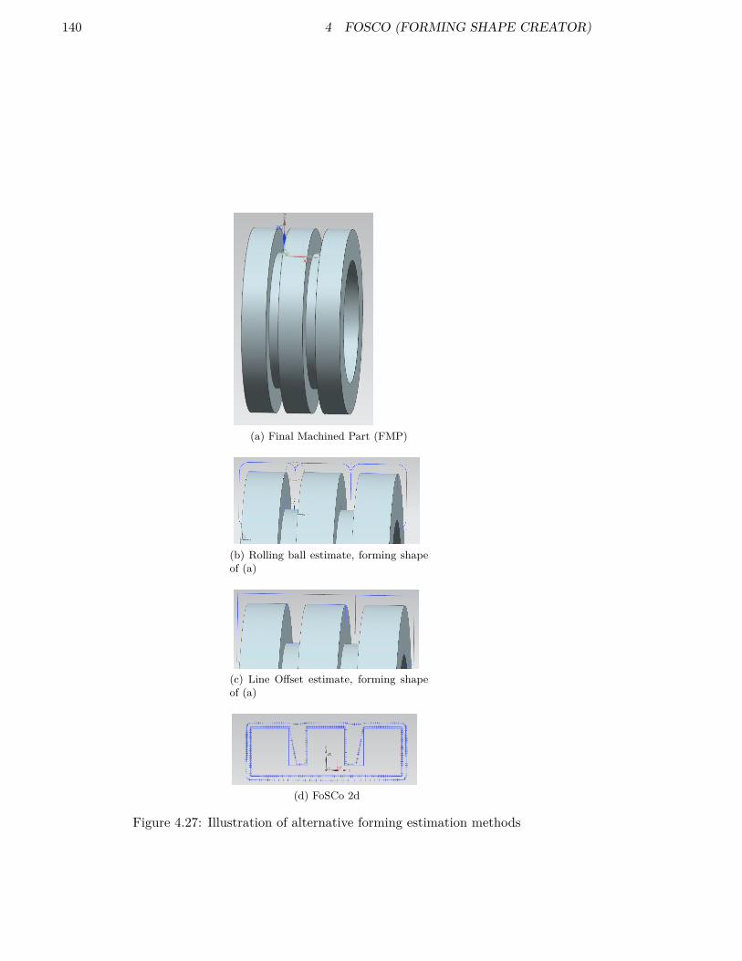
140 4 FOSCO (FORMING SHAPE CREATOR)
(a) Final Machined Part (FMP)
(b) Rolling ball estimate, forming shapeof (a)
(c) Line Offset estimate, forming shapeof (a)
(d) FoSCo 2d
Figure 4.27: Illustration of alternative forming estimation methods

141
5 Manufacturing Choice Optimisation and Sequencing Tool
5.1 Introduction to Manufacturing Choice Optimisation and SequencingTool (MCOST)
The objective of MCOST is:
Given the finished part geometry and tolerance data, parameterised as a set ofdesign features, and given the precursor shapes for one or more manufacturingstrategies (i.e. the choice of primary forming process) find the lowest costfeasible method of manufacture.
Thus MCOST is an optimiser around a feasibility and cost model which finds the optimummanufacturing route for a component after decomposing the design features into elementalfeatures. Elemental features would be, in extremis, features which cannot be representedby combinations of other, simpler, features.
MCOST has several tasks, it must:
1. Take a set of design features and their associated geometry and convert them intoelementary features (to be discussed in Section 5.7.3)
2. For GO iterations - select the manufacturing processes which comprise the most costeffective way to make all elemental features:
(a) Choose a set of manufacturing processes to make each elemental feature
(b) Amalgamate the sets of processes (create Complete Process Set)
(c) For GI iterations - sequence the processes to meet feasibility constraints:
i. Sequence the set of manufacturing operations (create Method ofManufacture).
ii. Check whether the sequence is feasible, if not return to i.A. Model the time of the sequence (operation time is assumed independent
of machine choice)B. Choose the machine and TAD (Tool Access Direction) for each operationC. Model the cost of the sequence
iii. Continue to optimise the sequence, return to i.
(d) Continue to optimise the choice of process sets, return to (a)

142 5 MANUFACTURING CHOICE OPTIMISATION AND SEQUENCING TOOL
5.2 Nomenclature
5.2.1 General Nomenclature
Symbol Meaning
FMP Final machined partFS Forming Shapeb1 time to cost model a single operationb2 average operation combinations per elemental featureb3 average operations per elemental featurec1 b1 · b2 · b3
GO Maximum allowable generations in the outer loop (Process selection)GI Maximum allowable generations in the inner loop (Operation sequencing)teval Time to cost model a method of manufactureX The matrix of numbers determining choices for manufacturing process selection
5.2.2 Scrap and rework calculation
Symbol Meaning
Pns,n Probability of not scrapping due to a single dimension (n) successPnso Probability of not scrapping as a result of a single operationPso Probability of scrapping as a result of a single operation = 1− Pnso
Pnr,n Probability of not reworking due to a single dimension (n) successPnro Probability of not reworking as a result of a single operationPro Probability of reworking as a result of a single operation = 1− Pnro
5.3 Definitions
Design Feature A feature used by a designer to achieve a certain objective (for example:affix to another component, provide structural rigidity, provide an aerodynamicsurface of a specified shape). Design features can be additive or subtractive.
Elemental Feature A feature which need not be broken down into other, simplerfeatures. Design features are composed of one or more elemental features.
Manufacturing Feature A feature created by a single manufacturing process. There is amany-to-many mapping between elemental and manufacturing features.
Manufacturing Operation A specific instance of a manufacturing process, operating ona specific elemental feature.
Manufacturing Process Any manufacturing process associated with the manufacture ofthe component, including inspection type operations.

5.3 Definitions 143
Word/Phrase Acronym MeaningManufacturing A manufacturing process such as
Process turning, milling, heating, forgingManufacturing An instance of a manufacturing process
Operation (for an elemental feature)Manufacturing The primary manufacturing process (the process
Strategy used to make the precursor shape)Process Set PS All of the manufacturing operations used for
an elemental featureComplete Process CPS All of the manufacturing operations used
Set for the componentFinal Machining FMP A manufacturing process which can create a
Process feature to within all defined tolerancesMethod of
ManufactureMoM The complete process set after sequencing
Route Creator RCS A datastructure which stores the CPS and theStructure precedence relationships between processes
Route Sequencing RSS A datastructure which stores the CPSStructure during the sequencing phase (inner loop)Best Inner BILC The lowest cost found in the currentLoop Cost optimisation for this CPS
Best Global Cost BGC The lowest cost found in the currentoptimisation
Parental Feature DFC Design Feature undergoing Conversion(to elemental features)
Table 5.1: Meaning of words and phrases used during the optimisation process
Manufacturing Strategy The class of manufacturing process associated with themanufacture of the precursor/forming shape, it is the primary additivemanufacturing process used for the component.
Process Set The set of processes necessary to manufacture all of the elemental featureson/in a component.
Process Sequence The process set constructed into a sequence of processes/operations.
KnowledgeBase A central database (Figure 5.1) which stores:
1. Design features
2. Elemental features
3. Design to elementary feature mapping
4. Manufacturing processes: their capabilities, variability, cycle time, costs,predecessors and successors
5. Machines: their location, cost rates, labour requirements and capabilities
6. Intra and inter factory transport costs

144 5 MANUFACTURING CHOICE OPTIMISATION AND SEQUENCING TOOL
Outer Loop The optimisation loop which constructs and modifies the process set inaccordance with the optimiser rules. Having completed the inner loop it identifieswhether to keep the previous process set or move to the new one. The dataassociated with the process set are stored in the RC (Route Creator) DataStructure.
Inner Loop The optimisation loop which operates fully within the outer loop. Itconstructs the process sequence from the process set and calculates times and costsfor each operation. The data associated with the process sequence are stored in theRS (Route Sequencing) DataStructure.
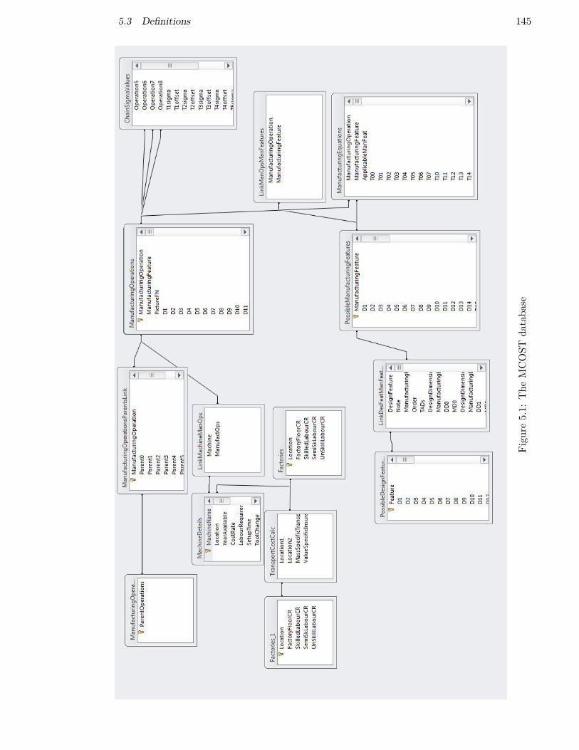
5.3 Definitions 145
Figu
re5.1:
The
MCOST
databa
se

146 5 MANUFACTURING CHOICE OPTIMISATION AND SEQUENCING TOOL
5.4 Justification for a holistic view
As can be seen from the literature review, there has been substantial research on theconstruction of manufacturing routes. However, most of this research begins with theassumption that the Complete Process Set (CPS) is already chosen and all that is necessaryis to sequence it to create a Method of Manufacture (MoM). This would only identify theglobal optimum MoM if the optimal Process Set (PS) for every feature was dependent onlyon characteristics known at the commencement of the optimisation. It will be shown in thissection that the optimal PS is partially dependant on the sequence of operations and thePS for other features, and thus a method which assumes that the CPS is already fixed mayfrequently find suboptimal solutions. Amongst other factors the optimal PS can depend on:
1. Tolerances (of feature and other features)
2. Geometry (of feature and other features)
3. Material (of the component)
4. Starting/precursor shape
5. Process sequence
Several of these responses are shown in the following section.
This can be explored on a simple feature of a ring of holes. Given a cost prior to theoperation, and a set of dimensions and tolerances, it can be determined whichmanufacturing process is the optimum method of manufacture for the given feature. Thisentails exploring which manufacturing processes give the lowest cost after completion of theoperation and taking into account the scrap rate. The equation used is a simplification ofthe equations stored in the manufacturing process database but is sufficient to demonstratethe aforementioned point. We can use an equation amalgamating the costs into a simplerequation rather than using the detailed cost equations present in the optimisation becausehere the breakdown is unnecessary. The equation used for the generation of Figure 5.2 is:
CO = (1 + FR) (CB + (T0 + TS)CR)− CB (5.1)
In the four graphs shown in Figure 5.2, the optimal process set for the elemental feature isthe lowest line at the point in the graph denoted by the independent variable.
Firstly exploring the effect on the operation cost (CO) of simply changing the number ofholes (Figure 5.2a). This will explore the effect of setup time (TS), operation time (TO)(number of holes multiplied by time per hole), and machine cost rate (CR). So drilling andreaming is optimal up to about 75 holes, then drilling is the least costly up to about 175

5.4 Justification for a holistic view 147
holes when the low value of the part and the higher probability of scrap fails to outweighthe cost saving from a less accurate process. Finally at around 170 holes the benefits oflaser drilling outweigh the additional setup cost. It should be noted that in themethodology at present there is the assumption that the probability of creatingscrap/rework is independent of the number of elements (such as holes), this is clearly untruein some cases and the need to improve this is highlighted in Section 6.5, however it doesnot invalidate the argument presented in this section or this thesis. The effect espousedupon will still be present albeit at potentially different points of the independent variable.
Secondly, the effect of a change in the prior cost (Figure 5.2b). The prior cost (CB) is thecost incurred getting the component to its current state, which will be wasted if scrap (witha scrap rate of (FR)) is generated in this operation. Rework rate has been ignored in thisexample, as this simply increases the operation cost and can thus be modelled in (CR) .
Thirdly and finally, exploring the response of the methodology to the previous machine inthe operation list. If the previous operation is conducted on a mechanical drilling machinefor reasons of size of the hole of the other hole based feature, the response of the nextoperation to number of holes is shown in Figure 5.2c, the mechanical drill should be usedunless the hole count exceeds 310. Assuming now that that the other hole feature, forreasons of tolerance, cannot be satisfactorily mechanically drilled, but must be laser drilled(Figure 5.2d), and must be conducted prior to the feature under investigation. Nowassuming that there are no constraints requiring separation of manufacturing of the twofeatures. The setup cost of the laser drilling method can now be zero, and the optimalmanufacturing process for any number of holes (in this example) is laser drilling.
The method presented in this section of the thesis will thus change the manufacturingmethod in response to both feature level stimuli and route level stimuli, the latter being ofparticular interest and novelty. All of the above changes result in a change in the choice ofmanufacturing method for a given feature. The first is a change internal to the feature butthe others are external and are therefore harder to predict as a result of epistasis. Thereare many other responses of the optimum manufacturing method for a feature in responseto both internal (to the feature) changes and external.
It can therefore be seen from the examination of these cases that asking the question,“What is the least expensive manufacturing process for this feature?” is not at allstraightforward. the answer depends not only on the characteristics of the feature, but alsoon the preceding manufacturing route, both the immediately preceding operation and allothers, where a possibility of generating scrap exists. Given this logic it also follows thatthe optimal choice of process also depends on the immediate and subsequent downstreamprocesses. When this argument is accepted, it follows that a logic based process ofdecisions made on incomplete information but affecting subsequent decisions willsometimes fail to reach an optimal decision; this leaves exhaustive search and optimisationroutines, and exhaustive search rapidly becomes too large (Section 5.6) a computational
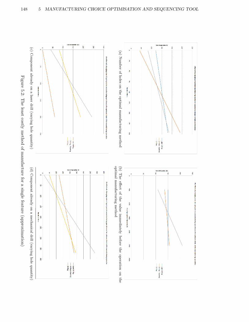
148 5 MANUFACTURING CHOICE OPTIMISATION AND SEQUENCING TOOL
(a)Num
berofholes
onthe
optimalm
anufacturingmethod
(b)The
effectof
thevalue
immediately
beforethe
operationon
theoptim
almanufacturing
method
(c)Com
ponentalready
onalaser
drill(varyinghole
quantity)(d)
Com
ponentalready
onamechanicaldrill(varying
holequantity)
Figure5.2:
The
leastcostly
method
ofmanufacture
forasingle
feature(approxim
ation)

5.4 Justification for a holistic view 149
problem to solve for all but the most simple test cases.
150 5 MANUFACTURING CHOICE OPTIMISATION AND SEQUENCING TOOL
5.5 Optimisation
Optimisation methodologies are extensively used to explore simulation/evaluationproblems where exhaustive search of a design space is intractable or infeasible. Some of thecommonly used optimisation routines which are used in this research are outlined below:
ArtificialNeuralNet A machine learning algorithm for machine decision making,constructs a decision tree which can be modified, usually using weighted branches.
GA A genetic algorithm, comes in many variants, inspired by natural selection, usuallynew individuals are created using recombination of pairs of individuals and mutationof chromosomes, a variant exists with a population size of one, described below.
RMHC A specific sub-category of a GA which has a population size of one thus makingrecombination of pairs impossible. This type of GA relies only on mutation and keepsthe new individual if it is better than the original, or discarding if it is not. There ismuch literature about the relative benefits of each type of GA. Initial tests wereconducted early on in the research which resulted in superior performance from theRMHC (i.e. fewer calls of the objective function necessary) however it is left to futurework to re-investigate.
SA Simulated Annealing, a search similar to an RMHC but which can descend to lowerfitness individuals with some probability, this probability of descending to lowerfitness will reduce over time, it should be considered complementary to otheroptimisation techniques as it does not specify the nature of the mutation, it onlymodifies the acceptance criteria.
5.6 Elemental features and computational limitations
As illustrated by Musharavati/Hamouda (2011) it is difficult to find an optimumprocess plan by testing all feasible solutions, the author’s own derivation of the size of thedesign search space is shown below.
The computational time taken for an exhaustive search of this problem is derived below:
teval = b1 · nops
sizeoptimisation = b2 · n · nops!
nops = b3 · n

5.6 Elemental features and computational limitations 151
Ttotal = sizeoptimisation · teval
So:
Ttotal = b2 · nfeatures · (b3 · n)! · b1 · b3 · n (5.2)
Ttotal = b1 · b3 · b2 · n2 · (b3 · n)!
Ttotal = c1 · n2 · (b3 · n)! (5.3)
Where:
Ttotal total time to run exhaustive search of the design search space
b1 time to cost model a single operation
b2 average operation combinations per elemental feature
b3 average operations per elemental feature.
c1 = b1 · b3 · b2, i.e. a constant determined by manufacturing knowledge.
n Number of features in the component to be cost modelled.
nops Number of operations in the manufacturing route.
So:
Minimising the number of elemental features is key to ensuring a rapid optimisation as thiswill reduce the size of the design space with a relationship as shown above, the timeincreases with n2 · (b3 · n)!. Given this relationship it can be seen that increasing thenumber of features will hugely increase the run time of the optimisation. Thus somefeatures which could be decomposed into simpler features are therefore better left in anon-simplified form. For example a slot is composed of multiple faces but this is anunnecessary increase in the number of features, indeed in this research even multiplesimilar features are treated as elemental features provided they share tool access directionsand are of a similar type.
It is of course true that an exhaustive search cannot reasonably be conducted on any butthe simplest components but given the high level of epistasis in this optimisation the totalnumber of evaluations necessary to achieve a reasonable chance of convergence to the

152 5 MANUFACTURING CHOICE OPTIMISATION AND SEQUENCING TOOL
global optimum will grow with an increase in the total number of possibilities.
In addition to the reduction in the number of elemental features other methods of reducingcomputational time are:
• Filtering out or repairing infeasible solutions
• Superior optimisers requiring fewer objective function calls
• Use of an objective function with a more rapid evaluation (i.e. a simpler and/or moreefficient cost model)
5.6.1 Features
Of particular interest in this research is the consideration of features. There is afundamental difference in thinking between design and manufacturing engineers, and it isthis difference which makes the process planning problem complex to solve.
Designers think of features in terms of solving fundamental engineering issues such as: thedirection and control of working fluids, the transfer and control of stress, control of fatigue,and resistance to heat, chemicals and erosion.
Manufacturers think in terms of achieving geometry to within tolerance, usually byremoving or forming material, or joining parts together by welding, riveting or bolting.
It is clear that the manufacturing process must be deduced by the methodology in order tomaintain flexibility, and we do not wish to filter out any potential solutions and given thatmanufacturing features are created by each manufacturing operation. The questiontherefore is how to define features such that the manufacturing method need not bepredetermined, and it is clear that a new type of feature must be defined since designfeatures themselves would introduce unnecessary complexity. To demonstrate this we cantake a set of n bosses with a hole in the centre such as in test case one (Section 1.8, Table1.2). This feature will at the very least require a hole making operation and some shapingor machining. The two processes are fundamentally different and need not be conductedconsecutively, in fact they are unlikely to be conducted consecutively because to do sowould increase the cost due to machine/tool changes.
The research thus introduces the concept of an elemental feature, a feature which can beproduced in one or more operations but need not be broken down into other, simpler,features in order to allow lower cost manufacturing sequences. When all elemental featuresof a design feature are combined the geometry of the combination is identical to that of thedesign feature.
Given the substantial level of research into feature recognition, it was decided that a

5.7 MCOST Structure 153
complementary method would be created; hence feature based manufacturing optimisationusing machine decision making. This will include a feature mapping from design toelementary features which could be replaced by feature recognition in future work. Adiscussion on features is presented later but a brief definition of the features to be used isshown in Section 5.3. Some feature recognition technologies recognise elemental featuresbut some recognise design features.
5.7 MCOST Structure
Written in C#, a schematic for the whole of MCOST is shown in Figure 5.3. The interfacesof MCOST with: the Access KnowledgeBase, Excel component data, and its own internalDataStructures are illustrated.
As can be seen MCOST is structured as: preliminary work; two optimisation loops, oneinside the other; and post-processing.
1. Preliminary work includes import of the KnowledgeBase and component data;conversion of design to elemental features and initialisation of the matrices for thefirst objective function evaluation.
2. The outer loop is tasked with selecting the manufacturing operations which comprisethe complete process set, identifying possible machines and TADs. It also calculatesscrap and rework rates and the operation precedence list and provides all thisinformation to the inner loop for sequencing operation.
3. The inner loop sequences these complete process sets to find the minimum costfeasible MoM.
4. Post processing includes bringing together the final results of the optimisation, andpreparing them for user interpretation. This includes showing the uncertainty withregards to times and costs of the manufacturing operations.
The reasoning behind the internal and external loops is that this structure allows continuityof optimisation. Given that not all complete process sets generated will have the samenumber of operations, and given that the number of operations for each feature may differ,if the complete process set is changed each time, it is challenging to preserve advantageousparts of the sequencing genome. It is possible that a good CPS will be disregarded throughan unlucky set of sequences which fail to maximise on its potential but it is thought(though not tested) that the benefits of continuity exceed this detriment. Future workcould be to create and test a methodology for preserving the aspects of the sequence whichcan be, whilst allowing the CPS to change every objective function evaluation.
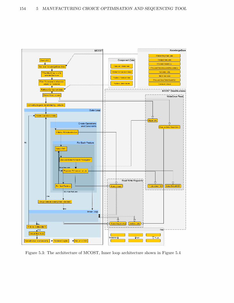
154 5 MANUFACTURING CHOICE OPTIMISATION AND SEQUENCING TOOL
Figure 5.3: The architecture of MCOST, Inner loop architecture shown in Figure 5.4
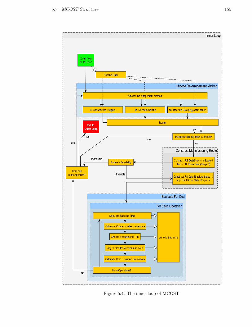
5.7 MCOST Structure 155
Figure 5.4: The inner loop of MCOST

156 5 MANUFACTURING CHOICE OPTIMISATION AND SEQUENCING TOOL
5.7.1 CAD geometry (NX Data) and MCOST Interface (NX Data to ExcelSpreadsheet)
Data from the NX component is exported to an Excel spreadsheet to interface withMCOST in order to allow the use of formulae when required. These data from NX aresimply a list of named dimensions.
In Excel the data are converted to a list of design features and their associated G&T(geometric and tolerance) data. There is also data pertaining to the component such asmaterial choice, production volumes and year of production which is relevant to cost butnot stored in the NX model.
This Excel spreadsheet is manually created but automated methods of creation do exist,including feature recognition or design using standard features. It needs to be created onlyonce per component template however; all components which can be made using that set ofdesign features can then be constructed from the template.
In this template there are also some constraints which must be created. These are theconstraints which exist between design features. For example a constraint may be that theholes in a set of bosses must be manufactured after the bosses themselves are created. Theformation of these constraints would be expected to be part of a feature recognitionalgorithm, if this methodology were to be integrated with one.
5.7.2 KnowledgeBase (Access database)
MCOST relies on a database (Figure 5.1) previously described. In more detail this contains:
• Data on machines and factories such as size, costs, energy consumption, operationsthat the machine can complete
• Process predecessors and successors and criteria if any exist for that relationship
• Process set variability
• Process time/cost equations
• Design features, elemental features and their mappings
After the KnowledgeBase and NX data is imported the KnowledgeBase is filtered to keeponly machines and process which are allowable (due to the year of productioncommencement and choice of suppliers).

5.7 MCOST Structure 157
5.7.3 Design to Elemental Feature conversion
A simple, one to many, user adaptable mapping is used for design to elemental featureconversion. A single design feature (DFC) is split into n elemental features, whereprecedences can be created between the different elemental features. Geometric andTolerance data of the elemental features are directly mapped from the G&T data of thedesign feature.
An example of the design feature dimensions and their conversion to elemental features fortest case one is shown in Figures 5.6, 5.7, 5.8. For many features the mapping values maybe the same, if this is the case it means that the design feature and elemental features areidentical. For others, generally more complex design features, the mapping values are notthe same. The information in these tables is as follows:
D-Values Dimensional values, contain only one double which corresponds to a particulardesign dimension.
T-Values Tolerance values, contain only one double which corresponds to a particulardesign tolerance.
L-Values Dimensional values, contain a list of doubles which correspond to a particulardesign dimension. Usually used for values which change over time (such as remainingdepth) where different manufacturing strategies will have differing values. Forexample a value in L0 of a multi stage groove (Figure 5.5) might be:CC,RF;1.06,5.81. This means that after centrifugal casting 1.06 mm remain formachining whist for Roll Forging 5.81 mm remain.
Figure 5.5: An example design feature: multi-stage groove
All these are defined for a particular design feature in the design feature table of theKnowledgeBase.

158 5 MANUFACTURING CHOICE OPTIMISATION AND SEQUENCING TOOL
(a)Design
Features:D-Values
(approximations)
(b)Elem
entalFeatures,D-Values
(approximations)
Figure5.6:
Testcase
onedesign
andelem
entalfeatures(D
-Values)

5.7 MCOST Structure 159
(a)DesignFe
atures:T-Value
s(app
roximations)
(b)ElementalFe
atures,T-Value
s(app
roxima-
tions)
Figu
re5.7:
Test
case
onede
signan
delem
entalfeatures(T
-Value
s)
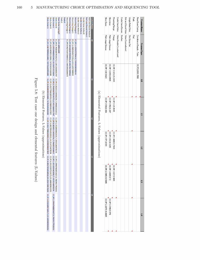
160 5 MANUFACTURING CHOICE OPTIMISATION AND SEQUENCING TOOL
(a)Elem
entalFeatures,L-Values(approxim
ations)
(b)Elem
entalFeatures,L-Values(approxim
ations)
Figure5.8:
Testcase
onedesign
andelem
entalfeatures(L-Values)

5.7 MCOST Structure 161
In addition to the dimensional mapping there needs to be a mapping of constraints. Allconstraints between DFC and other design features are copied to all elemental features andin addition new constraints between elemental features of DFC may be created accordingto KnowledgeBase rules.
5.7.4 Data-Structures Used (C# DataStructures)
Route Creator This structure stores the process set to be sequenced and evaluatedconstructed by the method listed in 5.8.1. It stores the operations to be used and theconstraints which exist.
Route Sequencing This structure stores the process route after sequencing, the choicesof machines and TAD and also the breakdown of costs.
Predecessor Neural Net (NN) There are two parts to this structure: the precedencespart and the successors part. When constructing the process set the predecessors andsuccessors for each operation on each feature are stored to reduce the calculationtime in future when the same query is made.
Scrap/Rework Structure Similar in reason to above
Feature Structure This keeps track of the dimensions of each feature during theproduction process. Features can have dimensions independent of forming process (Dvalues), tolerances (T values) and dimensions dependent on forming process (Lvalues). The L value format was developed to ensure that consideration of moreforming processes would not require re-coding of design features.
Equations This is to promote faster cost modelling as it stores co-efficients and indices indouble and integer form thus reducing conversion times. There is also a Booleanarray for if a cell is empty. This structure will be presented in more detail as it isfundamental to the speed of the optimisation and the method of data storage for thetime and cost calculations.

162 5 MANUFACTURING CHOICE OPTIMISATION AND SEQUENCING TOOL
5.8 MCOST Outer Loop
The MCOST outer optimisation loop is shown in Figure 5.3, the objective of the outer loopis to identify the optimal complete process set (CPS). It will be left to the inner loop toidentify the optimal MoM.
Optimisation is conducted using a random mutation hill climber (RMHC) adjusting valueswhich guide MCOST through the process set selection algorithm shown in Section 5.8.1,the optimisation of the random number matrix this algorithm uses is described in Section5.8.3.
A Genetic Algorithm (GA) rather that a RMHC was initially used but the RMHC showedmore rapid convergence, there may however have been better ways to code the GA thanused and it is left to future work to improve further on the optimisation routine used.
5.8.1 Process set selection
For each elemental feature a set of processes is required. This process set should make thefeature in the most cost effective way possible, however there is epistasis in this problem ashow another feature y is made will determine the optimal way to make feature x. This isdue to machine setup, transport between and inside factories and the effect of scrappingcomponents. For example a variable process which could be optimal at the beginning ofthe process route when the accumulated cost of a component is relatively low may not beoptimal later after substantial machining cost has been incurred.
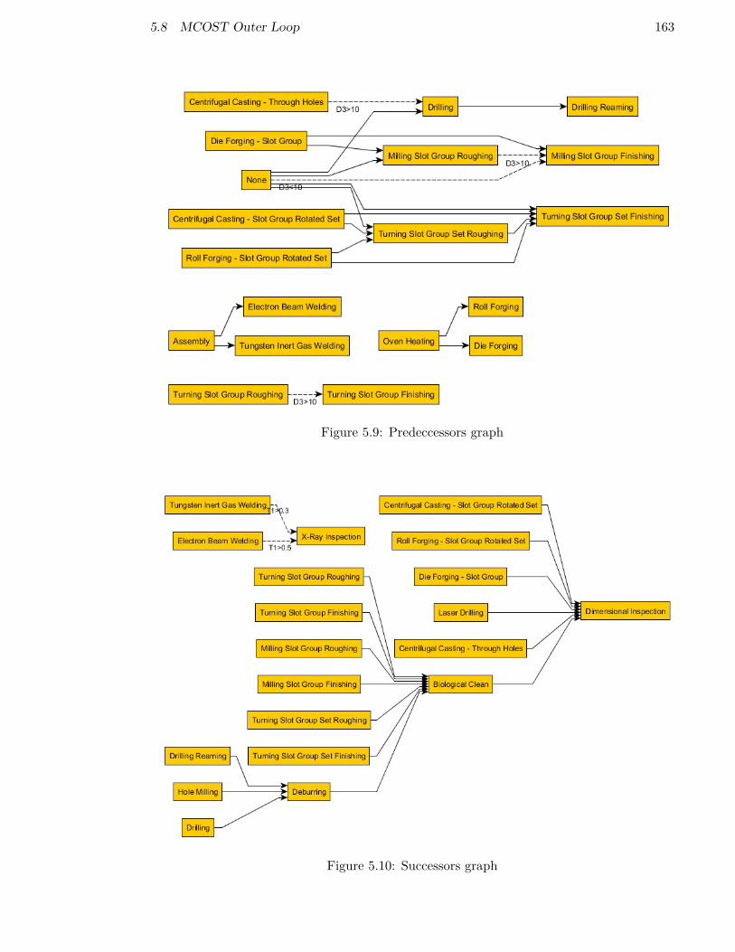
5.8 MCOST Outer Loop 163
Figure 5.9: Predeccessors graph
Figure 5.10: Successors graph
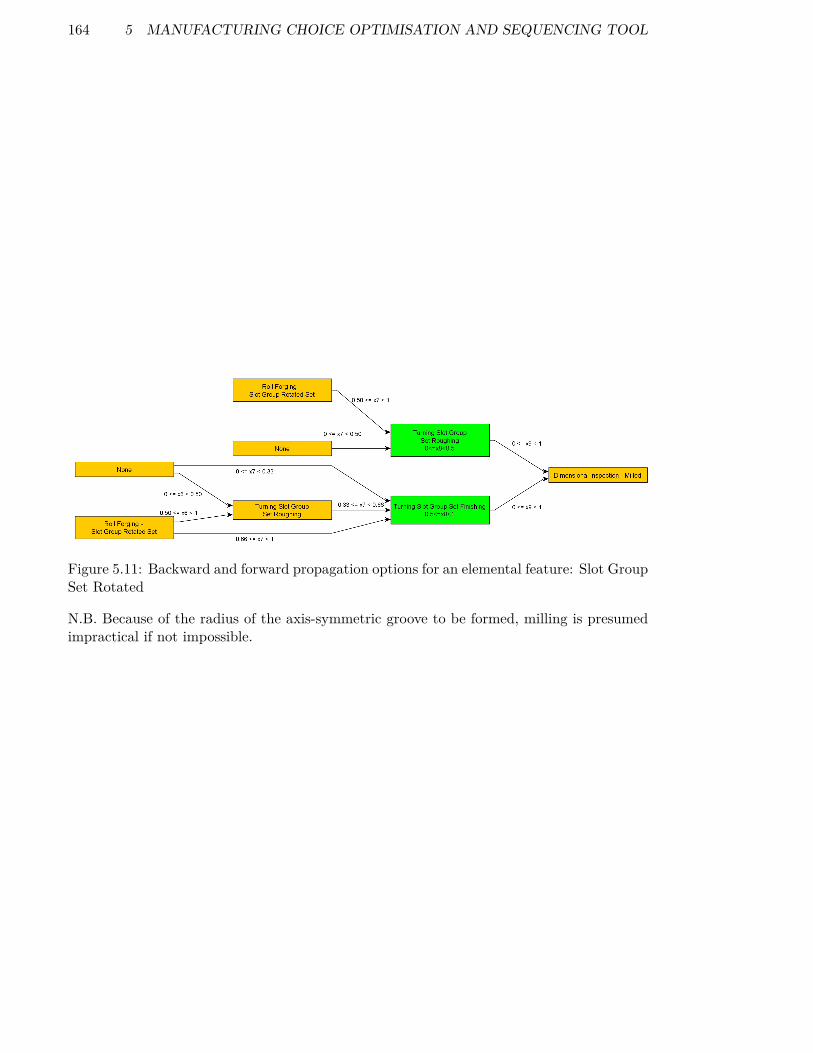
164 5 MANUFACTURING CHOICE OPTIMISATION AND SEQUENCING TOOL
Figure 5.11: Backward and forward propagation options for an elemental feature: Slot GroupSet Rotated
N.B. Because of the radius of the axis-symmetric groove to be formed, milling is presumedimpractical if not impossible.

5.8 MCOST Outer Loop 165
The concept of the FMP (Final Machining Process) is used here to mean a manufacturingprocess (usually chip forming but not necessarily) which creates a feature to within alldefined tolerances. From the FMP we can use backward and forward propagation toconstruct a chain of processes which are conducted on this elemental feature. For thismethodology it is also assumed that the FMP and any prior operations have an effect ondimensions and variability of the elemental feature and thus an effect on scrap and reworkwhereas subsequent operations do not. Numbers between zero and one are stored andcontrolled by the optimiser are used at each decision point, these numbers are stored in X,a matrix of size (nfeatures,19) and are mutated randomly prior to process set selection. Thecell of this matrix which refers to the choice of manufacturing strategy is not mutated.Where X is a row vector in matrix X, the central value (X[8] in each row determines theFMP (green in Figure 5.11), values X[<8] control the decision making for predecessorswhilst values X[>8] control the successors. Where a decision with one or more possibilitiesis encountered the choices are assigned equal selection bounds between zero and one. Thevalue in X[n] is used to choose and the options are stored for future queries. Once a ’None’process is reached or there are no predecessors/successors to choose from any remainingvalues in row X remain unused. The requirement for the ’None’ process stems from theoptionality behind predecessors, they are not necessary, and their inclusion may have abeneficial/deleterious effect on the cost.
This process creates the Route Creator structure shown in Figure 5.12. The list ofoperations is the grid view to the left, to the right is a grid view showing the list ofconstraints which must be met.
The operation ID is used primarily for constraint checking. An example from the Figure5.12 would be (Rear Outer Casting:0.7) It consists of three parts: A:B.C.
A The design feature from which the elemental feature is derived (Rear Outer Casting inthis example)
B The number of the elemental feature from the mapping, zero based (0 in this example)
C The operation number (7 in this example), if the OpId is:
8 the operation is the FMP,
< 8 the operation is a predecessor (e.g 7 is the predecessor to the FMP, 6 is thepredecessor to 7 if applicable etc.)
> 8 the operation is a successor (e.g 9 is the successor to the FMP, 10 is thesuccessor to 9 if applicable etc.)
All constraints are listed in the DataTable on the right of this figure
Constraints between design features have a different feature name (A), they are created bythe designer in the NX to MCOST interface file, an example of feature-feature constraints

166 5 MANUFACTURING CHOICE OPTIMISATION AND SEQUENCING TOOL
Figure5.12:
Atabulated
representationofthe
Route
Creator
Structure(R
CS)

5.8 MCOST Outer Loop 167
for test case one is shown in Figure 5.13, a solid line is binding on all operations associatedwith the feature. On the other hand a dashed line is binding only on operations up to andincluding the FMP, i.e. later operations such as clean up/inspection can be conducted later.
Figure 5.13: Feature-Feature constraints - Test case one
Constraints between different elemental features from the same design feature are definedby precedences created during the mapping from design to elemental features, they can beidentified by the same A value but a different B value. This relationship is created in theKnowledgeBase.
Finally constraints are created by the backward and forward propagation process, thesewill have identical A and B values but different C values (e.g. Rear Outer Casing:0.8before Rear Outer Casing:0.9 ).
There is currently no such thing as an immediate constraint (i.e. two operations must beconsecutive but this may be a useful addition to future work as this would limit the totalnumber of possible feasible combinations.

168 5 MANUFACTURING CHOICE OPTIMISATION AND SEQUENCING TOOL
5.8.2 Calculation of failure/rework probabilities
MCOST has data on the tolerance bounds allowed to various aspects of the feature and inaddition has process variability data relevant to the process chain which operates on thefeature. The probabilities of scrapping the part or reworking the feature are calculatedusing a multi-variant uncorrelated normal distribution, for which one, two and threedimensional examples are shown in 5.15, 5.16, 5.16, this method is capable of using morethan 3 dimensions but it becomes difficult to visualise. Once the process set rework/scrapvalues are calculated they are stored for future use. An extract of the process setvariability data is shown in 5.14.
It is assumed that for each defined tolerance on the feature, the process set chosen to makeit has a known variability. For each defined tolerance of the elemental feature theprobability of not scrapping the part is calculated. All of these not failing probabilities arethen multiplied to obtain the overall probability of success. This is subtracted from one togive the scrap probability due to the creation of a single elemental feature. All this is thenrepeated for rework instead of scrap.
Using the method of calculating the integral of a normal distribution developed byZelen/Severo (1964), for the calculation of rework and scrap probabilities we use thefollowing logic:
Pnso =m∏
n=1Pns,n (5.4)
Pnro =m∏
n=1Pnr,n (5.5)
Pso = 1− Pnso (5.6)
Pro = 1− Pnro (5.7)
Where
Z =∣∣∣∣ SigmaDesignToleranceSigmaMachiningVariability
∣∣∣∣ (5.8)
K = 11 + a0Z
(5.9)

5.8 MCOST Outer Loop 169
Figure 5.14: A sample of process set variability data
Figure 5.15: One dimensional normal distribution with scrap/rework (red/amber) regionsshown
Pnx,n = 1−( 1√
2π
)e
(− Z2
2
)(a1K + a2K
2 + a3K3 + a4K
4 + a5K5); (5.10)
Where
a0
a1
a2
a3
a4
a5
=
0.23164190.31938153−0.3565637821.781477937−1.8212559781.330274429
It is appreciated that this will double count the corners of the graphs as where a part ifscrapped in one dimension it will clearly not be reworked in another but for reasonablycapable processes it is thought that the effect of this slight over-calculation of rework istrivial and in any case this section of the code is modular and stores the results, thusnegating the need for a complete recalculation every iteration of the outer loop, this allowsthe potential for more complex and expensive methods of correlated multi-variant normaldistributions (MVNDs), for example.
It is also noted that work was conducted concurrently at the University of Southampton(Dodd, 2015) to calculate scrap and rework probabilities of correlated MVNDs and thereis the potential at a later stage to implement this work within MCOST.

170 5 MANUFACTURING CHOICE OPTIMISATION AND SEQUENCING TOOL
Figure 5.16: Two dimensional normal distribution with scrap/rework (red/green) regionsshown
Figure 5.17: Three dimensional normal distribution with the acceptable region shown (thered cube)
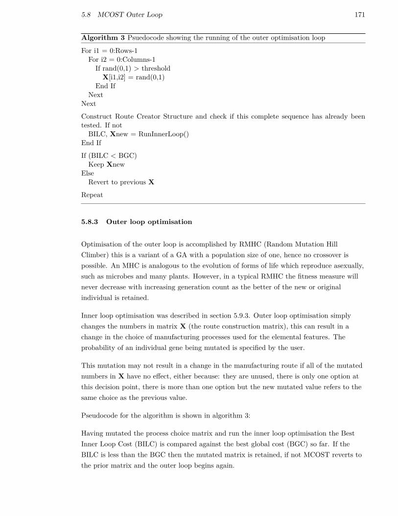
5.8 MCOST Outer Loop 171
Algorithm 3 Psuedocode showing the running of the outer optimisation loop
For i1 = 0:Rows-1For i2 = 0:Columns-1If rand(0,1) > thresholdX[i1,i2] = rand(0,1)
End IfNext
Next
Construct Route Creator Structure and check if this complete sequence has already beentested. If notBILC, Xnew = RunInnerLoop()
End If
If (BILC < BGC)Keep Xnew
ElseRevert to previous X
Repeat
5.8.3 Outer loop optimisation
Optimisation of the outer loop is accomplished by RMHC (Random Mutation HillClimber) this is a variant of a GA with a population size of one, hence no crossover ispossible. An MHC is analogous to the evolution of forms of life which reproduce asexually,such as microbes and many plants. However, in a typical RMHC the fitness measure willnever decrease with increasing generation count as the better of the new or originalindividual is retained.
Inner loop optimisation was described in section 5.9.3. Outer loop optimisation simplychanges the numbers in matrix X (the route construction matrix), this can result in achange in the choice of manufacturing processes used for the elemental features. Theprobability of an individual gene being mutated is specified by the user.
This mutation may not result in a change in the manufacturing route if all of the mutatednumbers in X have no effect, either because: they are unused, there is only one option atthis decision point, there is more than one option but the new mutated value refers to thesame choice as the previous value.
Pseudocode for the algorithm is shown in algorithm 3:
Having mutated the process choice matrix and run the inner loop optimisation the BestInner Loop Cost (BILC) is compared against the best global cost (BGC) so far. If theBILC is less than the BGC then the mutated matrix is retained, if not MCOST reverts tothe prior matrix and the outer loop begins again.

172 5 MANUFACTURING CHOICE OPTIMISATION AND SEQUENCING TOOL
5.9 MCOST inner loop
A schematic for the inner loop of MCOST is shown in Figure 5.18, the objective of theinner loop is to identify the optimal order of manufacturing operations by optimising andcost modelling the possible methods of manufacture (MoM) available from the currentcomplete process set. Clearly the number of possible MoM is equal to the factorial of thenumber of operations, although many of these will be infeasible, however computationaltime must still be invested to discover whether they are feasible or not.
5.9.1 Repair function
Given the number of constraints which exist, it is likely that a mutated individual, evenone from a feasible parent, will be infeasible. To prevent excessive computation thereforeafter mutation, and during initial route construction, a repair function is executed on thechromosome.
1 Forming Method Grouping This shifts all operations related to the formingoperation to the start of the process sequence, thus satisfying constraint one (seeSection 5.9.4).
2 Constraint Swap This swaps the positions of any pairs of manufacturing operationswhich breach their individual precedence constraints (see Section 5.9.4).
5.9.2 Initial process sequence initialisation
The start of the process sequencing algorithm is conducted as described below.
To begin with the processes are simply placed in an order determined by how they weregenerated by the outer loop. Effectively this means the sort will be by elemental featureand within this FMP, predecessors in reverse order, then successors. Clearly this will onlygenerate a feasible route where no predecessors exist to any of the FMPs, and all feature tofeature precedences are fortuitously met.
The repair function is then run, this will find a feasible solution, if at least one exists, forthe process set chosen. If no feasible solution is possible after the first instance of therepair function the algorithm reverts to the process set selection phase.
5.9.3 Process sequencing
The optimisation loop is then run. It is comprised of two more methodologies in aniterative loop to find the optimum sequence.

5.9 MCOST inner loop 173
Figure 5.18: The inner loop of MCOST

174 5 MANUFACTURING CHOICE OPTIMISATION AND SEQUENCING TOOL
1a Random re-sequencing This is a random rearrangement to attempt to reduce costusing random methods to break out of local optima, it works in a similar way to aplaying card shuffle, by moving a section of the integer list from where it is tobetween two other values, for example 1,2,3,4,5,6,7,8,9,10 ,11,12 could become1,2,3,8,9,10 ,4,5,6,7,11,12. The purpose of this algorithm is to attempt to keepbeneficial groups together once they have been discovered.
1b Machine This is a local search based on the assumption that grouping operationswhere the same machine is required will have the effect of minimising setups andtransport and thus the costs associated with them.
1c Machine and TAD Grouping Similar to 1b this groups operations where the samemachine and TAD are required, it is expected to have the same effect as 1b but witha further reduction in setup due to no change in component/machine orientation.
After each iteration of one of these operators the repair algorithm previously described isrun. The output from the two rearrangement algorithms followed by repair is a sequence ofconsecutive integers between zero and the number of operations:
After each rearrangement there is a multi-stage process test feasibility and cost, this is tomaximise the computational efficiency of the algorithm. It begins with the RCS and asequence of integers containing 0 to n and follows algorithm 4:
Algorithm 4 Feasibility and cost modelling of potential MoM
If sequence has not already been evaluated:Import only the OperationID Column (Figure 5.19).If the MoM is feasible (all constraints are satisfied)Import all other non calculated columns (shown in Figure 5.19).Calculate baseline time for all operations.Choose Machines and TADs using DTMS (Section 5.9.10).Calculate other times and all costs (creates Figure 5.21).
End If
In this way the most computationally expensive parts of the algorithm (particularly thecost/time modelling but to a lesser extent the feasibility check) are conducted only if theMoM has not already been checked.
5.9.4 Feasibility Analysis
Constraint analysis: A feasible manufacturing route will have a fitness value of zero.Fitness is calculated by querying whether the forming process operations occupy the initialpositions of the operation sequence, if they do not 15 is subtracted from the total.Secondly all predecessor constraints (Figure 5.12) are checked and one is subtracted fromthe fitness for each constraint breached. If the fitness is equal to zero, does the algorithm

5.9 MCOST inner loop 175
Figure 5.19: A tabulated representation of the Route Sequencing Structure (RSS) beforetime modelling, DTMS and cost modelling
proceed to the time and cost modelling stages, otherwise it returns to re-sequencing. Thisstep could be encompassed within the repair algorithm but remains separate as nosignificant advantage is derived from doing so and it remains a secondary check.
5.9.5 Equation Structure
M is a matrix specific to a manufacturing process for a defined feature type and costcategory or time. The actual equations structure which stores all the matrices has multiplearrays for each M to allow faster computation:
• A Boolean array identifying whether a particular cell is empty
• A Boolean array identifying whether a particular cell contains a double
• A Double array only populated for values which can be stored as doubles
• An Integer array where reference to a specific dimension, tolerance or machineattribute is required.
• A String array for values which cannot be stored in other, faster formats
• A List array for easy reference to the encoded functions.
• A List array for L-Values
176 5 MANUFACTURING CHOICE OPTIMISATION AND SEQUENCING TOOL
Available functions include sum, mean, difference, rounding and power functions, these areexpandable only by modification of the C# source code.
For example a function might consist of the text Fdiff,D1,L1:CC which would readD1-L1:CC where:
1. D1 would read the D1 value of the elemental feature to which the operation relates
2. L1:CC would read the L1 value of the elemental feature corresponding to centrifugalcasting.
The equations are taken from an access database, the reason being that this aids updatingof the equations by non programmers, and network deployment. There are three feasiblemethods of calculation of costs and times, each with unique advantages and limitations:
Non-compiled code Using an interpreted language such as VBA, Matlab or even Excelspreadsheets would be possible, but slow, hindering the optimisation processparticularly if calls to external programs are required.
Compiled equations within source code This is the fastest method, requiring hardcoded equations within the base software. However, a new manufacturing process ormodification to an existing process requires redeployment of the complete software,probably across a company’s network. In addition this approach would need the usersto be proficient coders which experience shows is a rare skill combination.
Hybrid Using hard coded equations but pulling in co-efficients from a centralised databaselimits flexibility but does not require software expertise to update the equations.
Compile at run time A language such as python could be used which compiles at first runtime, combines the advantages of: speed at run time and flexibility but retains thedisadvantage of requiring people of moderate programming skill to update, also raisespotential deployment issues for large organisations. Probably the best option butwould carry little advantage in terms of the proof of concept so is left as future work.
The hybrid approach is followed, flexibility is provided by allowing functions to be nestedwithin the co-efficients of the equation. These functions are hard-coded within the mainprogram and expansion of these in an industrial setting would cause disruption but shouldbe infrequently.
5.9.6 Volume Modelling
Volume Modelling calculates the volume removed or added in a manufacturing process. Itis calculated using an equation of the form:

5.9 MCOST inner loop 177
Volume = f (D,L) =4∑
m=0
( 7∏n=0
(Mm,n))
(5.11)
The values four and seven have been found to be sufficient to allow enough flexibility in theequations.
Where Mm,n can be: a coefficient, a dimension or tolerance of the feature (D, L, or T ), adimension or tolerance of the component (G), a characteristic of the machine (M), or afunction taking inputs of the aforementioned types. The same equation is used to calculatethe time and remaining cost categories (Sections 5.9.7 5.9.11).
An example of M for the volume calculation for process Milling Slot Group Finishing is:
M =
D1 D2 D3 D4D5 D6 D7 D8D9 D10 D11 D12D13 D14 D15 D16D17 D18 D19 D20
A blank entry in M0,0 ensures that the entire equation is assumed to be zero.
A blank entry in Mm,0 ensures that the row m is assumed to be zero.
A blank entry anywhere else is treated as a one.
Thus this calculation is equivalent to:
(D1 ×D2 ×D3 ×D4 × 1× 1× 1× 1)+ (D5 ×D6 ×D7 ×D8 × 1× 1× 1× 1)
+ (D9 ×D10 ×D11 ×D12 × 1× 1× 1× 1)+ (D13 ×D14 ×D15 ×D16 × 1× 1× 1× 1)+ (D17 ×D18 ×D19 ×D20 × 1× 1× 1× 1)
5.9.7 Time Modelling
Time modelling calculates the baseline time of an operation. It is calculated using thesame equation as the volume calculation in Section 5.9.6 but with the added option toreuse the calculated volume:
Time = f (D,G,L,M, v) =4∑
m=0
( 7∏n=0
(Mm,n))
(5.12)
178 5 MANUFACTURING CHOICE OPTIMISATION AND SEQUENCING TOOL
Where Mm,n can be: a coefficient, a dimension or tolerance of the feature (D, L, or T ), adimension or tolerance of the component (G), a characteristic of the machine (M), theadded or removed volume, or a function taking inputs of the aforementioned types. Thesame equation is used to calculate the remaining cost categories (5.9.11).
An example of M for the time calculation for process Milling Slot Group Finishing is:
Time = TimePerCubicMM · v
Where:
• v is the added or removed volume (previously calculated)
• TimePerCubicMM is extracted from a lookup table in the KnowledgeBase and is itselfa function of the hardness of the material and the type of manufacturing process.
5.9.8 Feature Modification
Conducted during the same calculation loop as the volume and baseline time calculationsare feature modification actions.
If the process modifies the feature, for example reducing the depth of it if aforming/cutting operation is used, then this occurs at the same time as the time calculated.The state of all features after each stage of the manufacturing process is stored so when thecost modelling is conducted the change in features need not be recalculated. In addition ifthe feature affects the T.A.D.s available to other features then their parameters aremodified at this point. This is done by identifying the modification (m) to the TAD andfeature (x) for which the modification takes place. MCOST then searches through theoperations list for all operations on x and modifies their allowed TADs to include m.
Finally it is noted that the cost of scrapping a component will only be known once a defectis discovered, thus during this stage of modelling the probability of failure is moved to thenext operation on the feature IFF the current machine is incapable of discovering thedefect. If there are no more operations on the feature an error is thrown. Furtherimprovements could be to define a variable capability to inspect for defects i.e. allmachines can detect defects at some pre-defined level of resolution.
5.9.9 Stored Time Values
Multiple times are derived from the baseline time and stored in a vector for the costanalysis later, they are:

5.9 MCOST inner loop 179
Baseline time The time of the operation without considering the effect of tool accessdirection (TAD). Calculated using formula Equation 5.12 Section 5.9.7.
Operation time The time of the operation after considering the effect of TAD.Calculated using a lookup table for manufacturing operation and TAD and applyinga factor to Baseline time.
Setup time The setup time of the machine, either a full setup, change in operation orchange in TAD (all machines have values for these categories).
Total time Setup time + Operation time.
Rework time Rework probability · Total time.
It is assumed that the rework is not discovered until the component has beenremoved from the machine.
Time Inc Rework Total time + Rework time.
These time values are calculated during the cost modelling stage (after DTMS, Section5.9.10) rather than the time modelling because they may depend on the choice of machineand TAD where a choice exists.

180 5 MANUFACTURING CHOICE OPTIMISATION AND SEQUENCING TOOL
5.9.10 DTMS (Dynamic Tool access direction and Machine Selection)
DTMS is an iterative method designed to identify the optimal machine and TAD (ToolAccess Direction) to use from the options available as shown in Figure 5.19.
It uses exhaustive search the possibilities within a segment of the process sequencingstructure to minimise the cost of an operation, taking into account the previous operationand the possibilities for the next operations, it relies upon knowing the times of past,current and future operations and hence must be run after the time modelling. The searchspace of each iteration of DTMS is shown in Figure 5.20, and it is run for eachmanufacturing operation in the MoM. In essence each iteration of DTMS 6d constructs asix dimensional array considering all possible combinations of machine choice and TAD forthe current operation and two future operations. The equation used to populate each cellof the array is shown in Figure 5.20, which takes into account the machine and TAD choicefrom operation n− 1 to n+ 2 inclusive. It then searches the array to find the minimumcost combination and returns the optimal choice of machine and TAD for operation n. Itwas stated in Section 5.4 that a logic based approach such as this one would not find theoptimal in a select group of test cases and this is correct, however the further into thesuccessive operations this approach looks, the less likely this sub optimisation becomes,hence the trade-off becomes a choice between a better but more costly evaluation of thecurrent method of manufacture, or allowing more evaluations to explore more methods ofmanufacture, assuming a given availability of computational resource. It is left to futurework to determine the optimal size of this evaluation, but it will of course depend on thespecific test case.
DTMS uses an amalgamated cost rate considering depreciation, labour and power for morerapid evaluation than if they were considered separately although this comes at theexpense of some accuracy in costs such as material costs and other which could depend onmachine choice.
5.9.11 Cost Modelling
Cost = f (D,G,L, T,M, v) =x∑
m=0
( 7∏n=0
(Mm,n))
(5.13)
Cost modelling for each operation is run immediately after running DTMS for thatoperation. For many of the cost categories the same equation format as the time modelling(Section 5.9.7) is used but with the added option of using the time values (OpTime, setuptime, total time). The costs are calculated using this method for the following categories:
• Labour
• Tooling
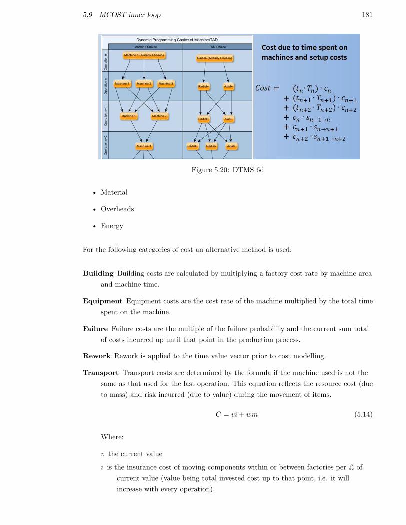
5.9 MCOST inner loop 181
Figure 5.20: DTMS 6d
• Material
• Overheads
• Energy
For the following categories of cost an alternative method is used:
Building Building costs are calculated by multiplying a factory cost rate by machine areaand machine time.
Equipment Equipment costs are the cost rate of the machine multiplied by the total timespent on the machine.
Failure Failure costs are the multiple of the failure probability and the current sum totalof costs incurred up until that point in the production process.
Rework Rework is applied to the time value vector prior to cost modelling.
Transport Transport costs are determined by the formula if the machine used is not thesame as that used for the last operation. This equation reflects the resource cost (dueto mass) and risk incurred (due to value) during the movement of items.
C = vi+ wm (5.14)
Where:
v the current value
i is the insurance cost of moving components within or between factories per £ ofcurrent value (value being total invested cost up to that point, i.e. it willincrease with every operation).

182 5 MANUFACTURING CHOICE OPTIMISATION AND SEQUENCING TOOL
CHENGDU DERBY HUCKNALL KHI SCAMCHENGDU 0.01, 0.001 2, 0.05 2, 0.05 2, 0.05 2, 0.05DERBY 2, 0.05 0.01, 0.001 0.5, 0.01 0.5, 0.01 0.5, 0.01
HUCKNALL 2, 0.05 0.5, 0.01 0.01, 0.001 0.5, 0.01 0.5, 0.01KHI 2, 0.05 0.5, 0.01 0.5, 0.01 0.01, 0.001 0.5, 0.01
SCAM 2, 0.05 0.5, 0.01 0.5, 0.01 0.5, 0.01 0.01, 0.001
Table 5.2: Co-efficients of cost of transport between selected factory pairs - fictitious valuesonly
w is the current mass
m is the resource cost of moving components within or between factories per kg
i and m are defined in the table below for selected factory pairs
It is true that i and m this equation will not necessarily be valid for certain (particularlyurgent) transport requirements but it is a reasonable surrogate.

5.9 MCOST inner loop 183
Figu
re5.21
:The
RSS
aftertim
emod
ellin
g,DTMSan
dcost
mod
ellin
g

184 5 MANUFACTURING CHOICE OPTIMISATION AND SEQUENCING TOOL
5.9.12 Acceptance Criterion and elite tracking - Inner loop
Nomenclature
Value ExplanationCurrent Value The cost of the current evaluation of the objective functionStored Value The most recently accepted (by acceptance criterion) cost evaluationElite Value The lowest cost evaluation for this inner loop
Table 5.3: Nomenclature for acceptance criterion - Inner loop
Generally speaking a RMHC will only move towards a new solution when it is superior tothe current best solution. This means that if an area of low fitness must be traversed toreach a superior local optimum (or the global optimum), a fortunate mutation must berandomly selected. Simulated annealing is a technique which allows (with someprobability) an inferior solution to be selected. As the optimisation progresses thetemperature is lowered and lower fitness solutions are less likely to be accepted. Thistechnique allows a more global search at the beginning, but becoming a very local search atthe end of the optimisation. In this section the words fitness is measured in GBP and isequivalent to the cost of the component being modelled.
The simulated annealing test depends on the current baseline, i.e. the latest acceptableevaluation which this individual was mutated from, also known as the stored value. Theacceptance criterion is shown below:
Accept ife(− 4F
T ) > R
Where
R =A random number between zero and one
T =Simulated temperature
4F =Delta fitness, the fitness of the current evaluation minus the fitness of the storedvalue
The propability of accepting a new value, given a previous value and current simulatedtemperature is shown in Figure 5.22.
Elite tracking refers to the fact that when simulated annealing is used there is thepossibility that the current solution can move away from the best to date solution (Figure5.25), at a high temperature, it is then unable return to the best solution as thetemperature drops. Elite tracking simply returns to the best solution so far in the innerloop (the Elite Value, Figure 5.26) thus allowing further improvement. The criterion to

5.9 MCOST inner loop 185
Figure 5.22: Simulated Annealling probability of acceptance of new solution - Stored value100,000
return to the elite is simply a deviation (4FE) of three times the temperature T of the SAalgorithm.
Where
4FE =Delta fitness, the fitness of the current evaluation minus the fitness of the elite value

186 5 MANUFACTURING CHOICE OPTIMISATION AND SEQUENCING TOOL
5.10 Calibration of MCOST KnowledgeBase
There are two key points determining the success or failure of MCOST as a methodology.
1. Is it finding the optimal manufacturing route or is it better than existing comparablemethods.
2. Is the cost that it calculates for the optimal route correct or better than existingcomparable methods.
3. Is it finding it as rapidly as possible or at least better than existing comparablemethods.
Clearly if the cost calculations are incorrect MCOST’s deductions for the optimal route ishighly likely to be incorrect, and even if it is correct it will not be believed. Calibration ofthe time and cost equations is the most important aspect of the cost modelling. The mostimportant aspects of the cost modelling are:
Time calculation times of processes
Equipment cost caused by depreciation and time spent on machine
Labour Cost Proportional to time and related to skill level of operator(s)
Bought in cost from suppliers, difficult to break down
Thus it can be seen that the biggest issue will be a miscalculation of the process times andbecause of this, this was the most concentrated on aspect. These equations were importedfrom the Rolls-Royce VCMS (Vanguard Cost Modelling System) lookup table shown inFigure 1.11, after inverting the values to give a time per unit volume value.
Initial verification was conducted by comparing the times extracted from MCOST for TestCase One: ROC against the SAP manufacturing data for the same part (Table 5.8).
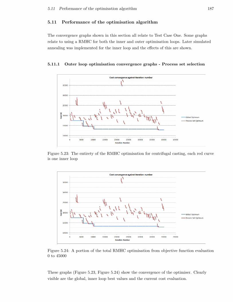
5.11 Performance of the optimisation algorithm 187
5.11 Performance of the optimisation algorithm
The convergence graphs shown in this section all relate to Test Case One. Some graphsrelate to using a RMHC for both the inner and outer optimisation loops. Later simulatedannealing was implemented for the inner loop and the effects of this are shown.
5.11.1 Outer loop optimisation convergence graphs - Process set selection
Figure 5.23: The entirety of the RMHC optimisation for centrifugal casting, each red curveis one inner loop
Figure 5.24: A portion of the total RMHC optimisation from objective function evaluation0 to 45000
These graphs (Figure 5.23, Figure 5.24) show the convergence of the optimiser. Clearlyvisible are the global, inner loop best values and the current cost evaluation.

188 5 MANUFACTURING CHOICE OPTIMISATION AND SEQUENCING TOOL
One of the biggest issues with optimisation of this complexity of design search space isidentification of when or if the global optimum is reached, this is a common issue withoptimisers exploring complex design search spaces with high levels of epistasis

5.11 Performance of the optimisation algorithm 189
5.11.2 Inner loop convergence graphs - Process sequencing
It is suggested in the literature review, that using simulated annealing in conjunction withan RMHC improves the convergence of the optimisation. The simulated annealing4
algorithm has been implemented on the inner loop of the optimisation and the results areshown in Figure 5.25. As can be seen from the figure, simulated annealing can drift awayfrom the optimum as improvement becomes more difficult in the later stages so areturn-to-best algorithm called Elite Tracking (ET) was implemented and its effect isshown in Figure 5.26. If the algorithm detects a cost increase between current cost andelite cost of more than three5 times current ’temperature’, it returns to the elite value forfurther improvement. In tabular form the results for with and without ET are shown inTable 5.27, assuming all else remaining equal apart from the random number generation forinner loop mutation. The marginal benefit of implementing elite tracking is around onepercent, which could make a substantial difference to a manufacturers profitability all elseremaining equal.
4It should be noted that a pure RMHC is a specific case of SA (i.e. where the ambient temperature iszero).
5This value can be explored to find an optimal value or on what the optimal value depends for the mostrapid convergence.
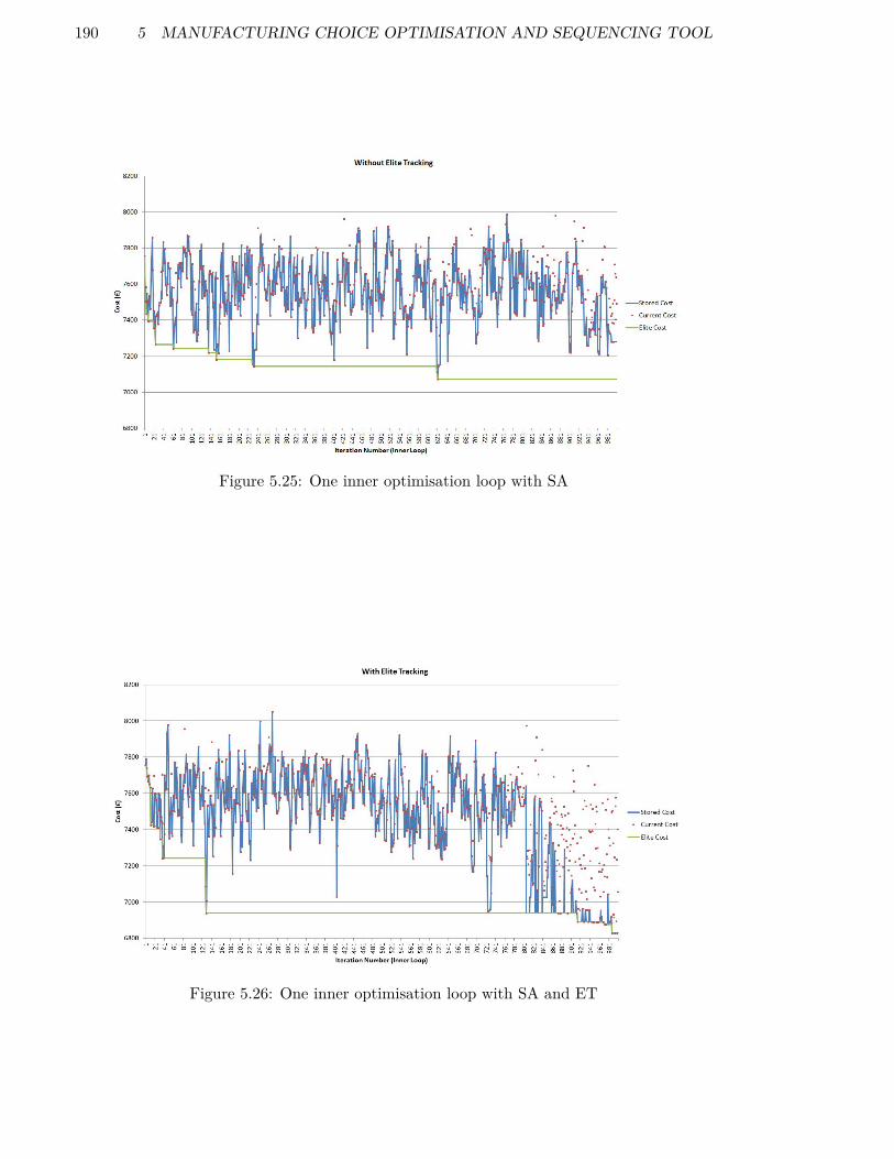
190 5 MANUFACTURING CHOICE OPTIMISATION AND SEQUENCING TOOL
Figure 5.25: One inner optimisation loop with SA
Figure 5.26: One inner optimisation loop with SA and ET

5.11 Performance of the optimisation algorithm 191
Figure 5.27: A tabular comparison of the same manufacturing processes optimised with orwithout elite tracking

192 5 MANUFACTURING CHOICE OPTIMISATION AND SEQUENCING TOOL
5.12 Results
It is clear that given the type of optimiser used, assuming more than one possiblepermutation of the objective function, an infinite number of iterations (in both the innerand outer loops) is necessary to guarantee that the global solution will be found. Howeverif the solution is desired in less than infinite time then an answer which is likely to be theglobal optimum, or is at least good enough, depending on the size of the design searchspace, must be accepted. It should be mentioned that only for test case zero wasconvergence actually reached.
Given this optimisation problem’s type as a discrete rather than continuous optimisationproblem, its quality can be determined by the frequency with which it can achieve theglobal optimum, if known, or how skewed the distribution of final results is. For example ifthe final result of exactly £8559 is achieved on 100 independent optimisation runs then itcan reasonably be assumed that either that value is the global optimum.
If the optimisation is run with insufficient iterations to consistently find the optimalsolution then a skewed normal distribution of final results (best result from the objectivefunction) to be achieved, truncated at the global optimum.
Where iteration count is specified, it refers to the number of objective function evaluations(i.e. G0 ·G1 except in exceptional test cases with only small numbers of options). In thesespecial cases, when the mutation operator failes to construct unique solutions repeatedly, itwill assume no more unique solutions exist and moves to the next loop.
5.12.1 Test Case Zero
Figure 5.28: Test Case Zero: Simplified Rear Outer Casing (ROC)
The total optimisation MCOST described in this section is run multiple times withdifferent (random) start points. Testing was conducted using differing numbers ofgenerations of the optimiser to show improved convergence to the global optimum if moregenerations are allowed. By simplifying the geometry the feature set, G&T data andprecedence list was contrived such that the global optimum was known to be £8559.
Each of the results generated by MCOST consists of the total cost of the manufacturing

5.12 Results 193
route, and a list of manufacturing operations with a complete cost breakdown for eachoperation, only the total cost is plotted in this graph (i.e. the lowest cost solution to theobjective function). If large numbers of optimisations are conducted it is expected that askewed normal distribution decay curve, truncated at the global optimum, will be shown ifall end results are plotted as a histogram as in Figure 5.29. Clearly at higher iterationcounts such at 10000 it is likely that all optimisation runs would find the global optimumof £8559.
Figure 5.29 shows the improvement towards more probability of finding the globaloptimum as the generation count is increased. If insufficient generations are used, thetruncation at the global optimum becomes less evident, as is shown for the test case oneresults in Figure5.31.
Figure 5.29: The spread of optimisation results varying with allowed generation count (StockMachining only)

194 5 MANUFACTURING CHOICE OPTIMISATION AND SEQUENCING TOOL
5.12.2 Test Case One
Figure 5.30: Test Case One: Trent 900 Rear Outer Casing (ROC)
A set of results for test case one is shown below. Three manufacturing strategies have sofar been modelled. For this test case ring roll forging, centrifugal casting and machinedfrom stock are shown.
The main output is a list of results from the optimisation (Table 5.4), each of these resultscontains a method of manufacture with a complete breakdown in costs, operation byoperation, an abridged version is shown in figure 5.32 and a breakdown of time spent onmachines for calibration with SAP data (Table 5.5). Table 5.4 can also be represented as agraph, as previously discussed in Section 5.12.1. Because insufficient time was allowed forconvergence of the results the truncation of the Gaussian distribution (at the globaloptimum) is not evident. We can however, see that on average Roll Forging has the lowestcost, followed by machined from stock and finally casting is the most expensive productionmethod for this component as specified.
Figure 5.31: Test Case One Results: A graph showing the end result of 16 optimisation runsfor each manufacturing strategy, raw data shown in Table 5.4

5.12 Results 195
Cost MS Cost MS Cost MS6574 Ring Roll Forging 8957 Stock Tube 9290 Centrifugal Casting7025 Ring Roll Forging 9138 Stock Tube 9422 Centrifugal Casting7319 Ring Roll Forging 9210 Stock Tube 9428 Centrifugal Casting7446 Ring Roll Forging 9254 Stock Tube 9691 Centrifugal Casting7466 Ring Roll Forging 9574 Stock Tube 9708 Centrifugal Casting7524 Ring Roll Forging 9592 Stock Tube 10210 Centrifugal Casting7585 Ring Roll Forging 9672 Stock Tube 10212 Centrifugal Casting7617 Ring Roll Forging 9785 Stock Tube 10291 Centrifugal Casting7685 Ring Roll Forging 9794 Stock Tube 10391 Centrifugal Casting7791 Ring Roll Forging 9822 Stock Tube 10398 Centrifugal Casting7834 Ring Roll Forging 9859 Stock Tube 10399 Centrifugal Casting7945 Ring Roll Forging 9897 Stock Tube 10421 Centrifugal Casting8410 Ring Roll Forging 9921 Stock Tube 10513 Centrifugal Casting8413 Ring Roll Forging 9937 Stock Tube 10664 Centrifugal Casting8422 Ring Roll Forging 10118 Stock Tube 10870 Centrifugal Casting8689 Ring Roll Forging 10782 Stock Tube 11531 Centrifugal Casting
Table 5.4: Set of cost estimates for test case one for each Manufacturing Strategy (MS)
Machine TAD Time
Pre-Forging Oven Radial+ 84
Hydraulic Press Radial+ 15
Roll Forger Radial+ 140
Roll Forger Radial- 2
Roll Forger Radial+ 6
Roll Forger Radial- 10
Mill/Drill/Turn Radial- 582
Mill/Drill/Turn Axial+ 274
Mill/Drill/Turn Radial- 82
Mill/Drill/Turn Axial- 252
Manual Deburring Radial+ 45
Manual Deburring Axial+ 43
Laser Driller Axial+ 51
Laser Driller Radial+ 12
Biological Clean Radial- 30
Robotic Inspection Axial+ 62
Robotic Inspection Radial+ 39
Robotic Inspection Radial- 93
Table 5.5: Time breakdown by machine and TAD of the lowest cost MoM (for Ring RollForging) shown in Table 5.4

196 5 MANUFACTURING CHOICE OPTIMISATION AND SEQUENCING TOOL
Machine TAD Time
Stock Supplier Radial+ 30
Mill/Drill/Turn Radial- 416
Mill/Drill/Turn Axial+ 173
Mill/Drill/Turn Radial- 323
Mill/Drill/Turn Axial+ 79
Mill/Drill/Turn Radial- 30
Mill/Drill/Turn Axial- 84
Mill/Drill/Turn Radial+ 22
Mill/Drill/Turn Axial- 105
Mill/Drill/Turn Radial+ 41
Mill/Drill/Turn Axial- 17
Mill/Drill/Turn Radial+ 205
Mill/Drill/Turn Radial- 3
Manual Deburring Radial+ 58
Manual Deburring Axial+ 35
Laser Driller Axial+ 45
Biological Clean Radial+ 30
Biological Clean Radial- 0
Biological Clean Radial+ 0
Biological Clean Radial- 0
Biological Clean Axial+ 0
Biological Clean Radial+ 0
Robotic Inspection Radial+ 53
Robotic Inspection Axial+ 40
Robotic Inspection Radial- 99
Table 5.6: Time breakdown by machine and TAD of the lowest cost MoM (for machinedfrom stock) shown in Table 5.4

5.12 Results 197
Machine TAD Time
Pre-Casting Oven Radial+ 91.81
Centrifugal Caster Radial+ 185
Centrifugal Caster Radial- 0
Centrifugal Caster Radial+ 0
Centrifugal Caster Radial- 0
Mill/Drill/Turn Radial- 176.61
Mill/Drill/Turn Axial- 9.92
Mill/Drill/Turn Radial+ 78.49
Mill/Drill/Turn Radial- 251.27
Mill/Drill/Turn Axial+ 188.41
Mill/Drill/Turn Radial- 138.07
Mill/Drill/Turn Axial- 29.93
Mill/Drill/Turn Radial- 2.93
Mill/Drill/Turn Radial+ 174.31
Mill/Drill/Turn Axial+ 71.57
Manual Deburring Radial+ 57.59
Manual Deburring Axial+ 35.1
Biological Clean Radial+ 30
Biological Clean Radial- 0
Biological Clean Radial+ 0
Biological Clean Radial- 0
Biological Clean Radial+ 0
Biological Clean Radial- 0
Biological Clean Axial+ 0
Laser Driller Axial+ 44.82
Robotic Inspection Radial- 75.17
Robotic Inspection Axial+ 11.3
Robotic Inspection Radial- 27.21
Robotic Inspection Radial+ 16.35
Robotic Inspection Axial+ 58.72
Robotic Inspection Radial+ 15.96
Table 5.7: Time breakdown by machine and TAD of the lowest cost MoM (for CentrifugalCasting) shown in Table 5.4

198 5 MANUFACTURING CHOICE OPTIMISATION AND SEQUENCING TOOL
Figure5.32:
Testcase
one:Rear
Outer
Casing,abridged
lowest
costpartialm
anufacturingroute
forcentrifugalcasting
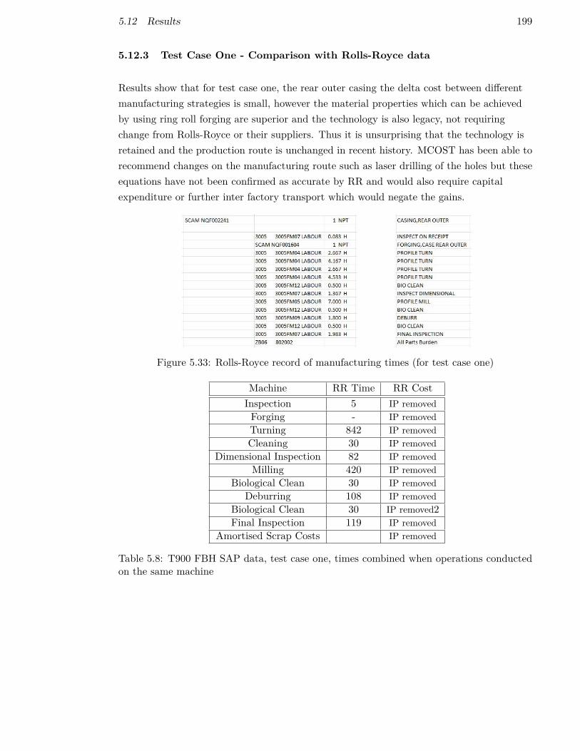
5.12 Results 199
5.12.3 Test Case One - Comparison with Rolls-Royce data
Results show that for test case one, the rear outer casing the delta cost between differentmanufacturing strategies is small, however the material properties which can be achievedby using ring roll forging are superior and the technology is also legacy, not requiringchange from Rolls-Royce or their suppliers. Thus it is unsurprising that the technology isretained and the production route is unchanged in recent history. MCOST has been able torecommend changes on the manufacturing route such as laser drilling of the holes but theseequations have not been confirmed as accurate by RR and would also require capitalexpenditure or further inter factory transport which would negate the gains.
Figure 5.33: Rolls-Royce record of manufacturing times (for test case one)
Machine RR Time RR CostInspection 5 IP removedForging - IP removedTurning 842 IP removedCleaning 30 IP removed
Dimensional Inspection 82 IP removedMilling 420 IP removed
Biological Clean 30 IP removedDeburring 108 IP removed
Biological Clean 30 IP removed2Final Inspection 119 IP removed
Amortised Scrap Costs IP removed
Table 5.8: T900 FBH SAP data, test case one, times combined when operations conductedon the same machine
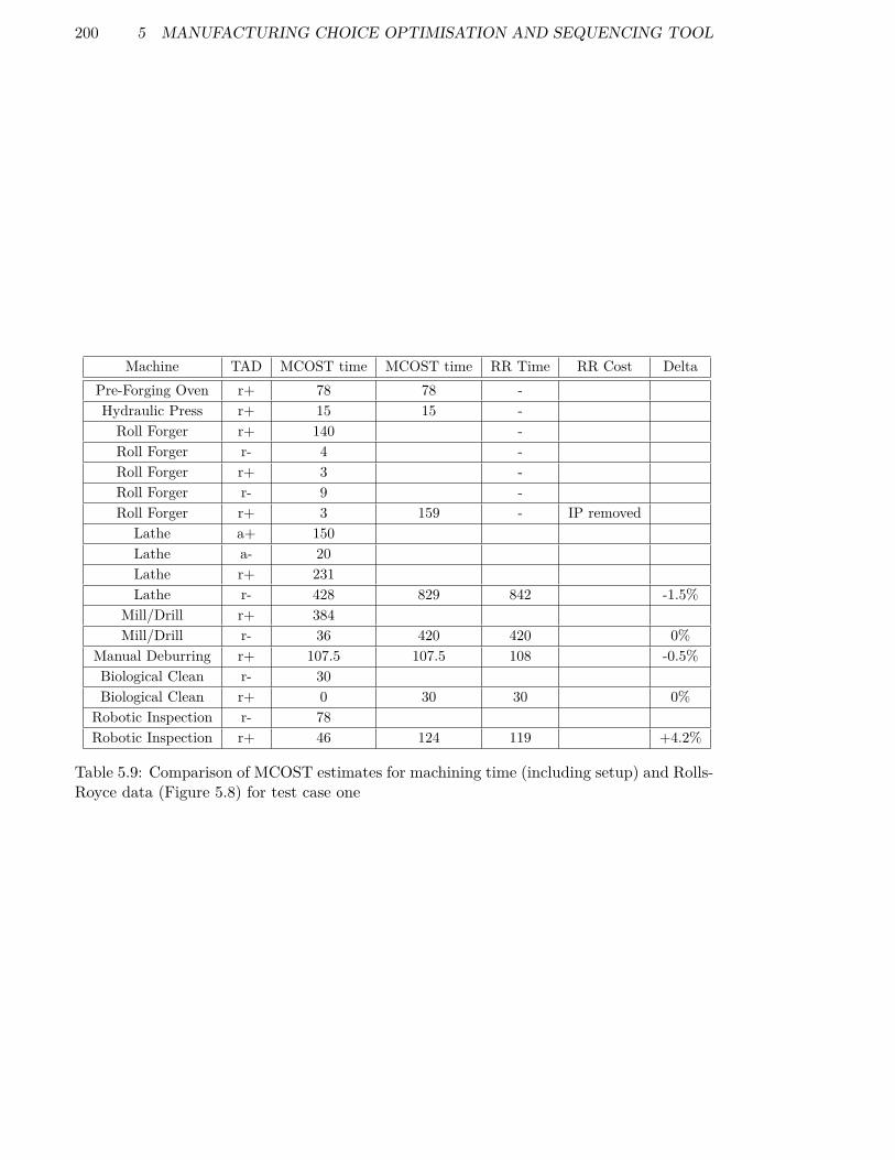
200 5 MANUFACTURING CHOICE OPTIMISATION AND SEQUENCING TOOL
Machine TAD MCOST time MCOST time RR Time RR Cost DeltaPre-Forging Oven r+ 78 78 -Hydraulic Press r+ 15 15 -Roll Forger r+ 140 -Roll Forger r- 4 -Roll Forger r+ 3 -Roll Forger r- 9 -Roll Forger r+ 3 159 - IP removed
Lathe a+ 150Lathe a- 20Lathe r+ 231Lathe r- 428 829 842 -1.5%
Mill/Drill r+ 384Mill/Drill r- 36 420 420 0%
Manual Deburring r+ 107.5 107.5 108 -0.5%Biological Clean r- 30Biological Clean r+ 0 30 30 0%
Robotic Inspection r- 78Robotic Inspection r+ 46 124 119 +4.2%
Table 5.9: Comparison of MCOST estimates for machining time (including setup) and Rolls-Royce data (Figure 5.8) for test case one

5.12 Results 201
5.12.4 Test Case Two
Figure 5.34: Test Case Two: Trent 700 Engine Section Stator (ESS)
Test case two (Figure 5.34) is usually die forged and machined to the finished shape.Figure 5.35 shows the a range of optimisation results using die forging as a manufacturingstrategy while Figure 5.37 shows the machine and TAD breakdown for the lowest cost dieforged method. Figures 5.38, 5.39 show an abridged breakdown of the data created byMCOST relating to Figure 5.37.
In addition the contrast between die forging and stock machining was explored. As can beseen, the best die forging method of manufacture is less costly due to the lower materialremoval volumes necessary, and lower input mass, although the cost of the input materialsis higher. However the optimisation pertaining to stock machining is more consistent dueto the smaller design search space it is exploring (there are fewer possible combinations).
The supplied cost for this component was £521 per vane in (2014). compared to MCOST’sbest prediction of £4212. The reason for the huge inaccuracy is that FoSCo 3d cannotcurrently represent (near) net shape manufacture (and indeed there is no point in it beingable to do so). For this component therefore both the predicted forging cost is too high andthe machining cost is also too high. On the aerodynamic surfaces only a polish is required,not milling operations as predicted by MCOST due to the incorrect FoSCo prediction.
Figure 5.35: Test Case Two: Range of optimisation results, all for Die Forging

202 5 MANUFACTURING CHOICE OPTIMISATION AND SEQUENCING TOOL
Figure 5.36: Test Case Two: Range of optimisation results including Die Forging and StockMachining
Figure 5.37: Test Case Two: Optimal MoM from Figure 5.35

5.12 Results 203
Figu
re5.38
:Te
stCaseTw
o:Abridgedop
timal
MoM
from
Figu
re5.37
(Colum
ns1-7)

204 5 MANUFACTURING CHOICE OPTIMISATION AND SEQUENCING TOOL
Figure5.39:
TestCase
Two:
Abridged
MoM
fromFigure
5.37(C
olumns
8-16)

5.12 Results 205
5.12.5 Minor Test Cases
MCOST was run on the minor test cases shown in Tables 1.4, 1.5 to demonstrate itsflexibility. It did not fail to give a response but was unable to accurately cost these parts.This was due to the fact that the manufacturing equations used were based onRolls-Royce’s experience of manufacturing large components. Smaller, more commoditisedcomponents such as these minor test cases would be procured from suppliers who wouldhave more experience in manufacturing smaller components and would be moreexperienced with optimal order quantities to minimise the cost of setup per component.This is an aspect of batch production and the suggestion to consider its inclusion is madein the conclusions.

206 5 MANUFACTURING CHOICE OPTIMISATION AND SEQUENCING TOOL
207
6 Conclusions
The previous sections in this thesis deal with:
Background Information A review of academic literature and the current state ofcommercial technology, the source data obtained from the industrial sponsor used inthis research.
Methodology Sections on the methodology and toolset created as a whole, then separatesections for the tool which creates the precursor shape estimate, and the tool formanufacturing optimisation.
6.1 Review of aims and objectives
The question to be investigated was:
Conducting manufacturing process selection prior to manufactuing sequencingin CAPP can lead to suboptimisation. Dynamic process selection, conductedwithin an optimisation will improve this, and thus allow superior decisionmaking by component designers and manufacturing experts.
It became apparent through the course of the research, that the optimal manufacturingprocesses depended to a significant extent on the precursor shape. Larger precursor shapes(such as those created by roll forging of high temperature materials) create a tendency touse processes with less smooth finishes and inferior accuracy, such as VIPER (VeryImpressive Performance Extreme Removal) grinding, but faster material removal rates.These may then require more precise finishing operations with improved surface finish.
The choice of manufacturing processes was a completely different type of question than theshape which would be generated by the precursor technology. Thus the research wasdivided into two sections, and two distinct, though complementary, tools were created: theForming Shape Creator (FoSCo), and the Manufacturing Choice Optimisation andSequencing Tool (MCOST). The purpose of FoSCo was to deduce potential precursorshapes. MCOST was developed to choose the manufacturing operations and their sequence.
The tasks required to satisfy the objective were covered by the two tools.
Task 1 To deduce the shape created using additive or forming processes (by which it ismeant casting, forging processes).FoSCo Section 4.
Task 2 To determine what possible manufacturing processes can be used to make theremaining features (i.e. any not already created by the additive or forming process.

208 6 CONCLUSIONS
MCOST Section Y. Implicit within the FMP, Predecessors and SuccessorsDataTables. Graphically shown in Section 5.8.1.
Task 3 To derive which possible manufacturing processes should be used to make theremaining features.Determined by the MCOST outer loop optimiser, this is a random mutation hillclimber which simply mutates the numbers in a matrix which determines the pathfollowed through the predecessor’s and successor’s tree illustrated in Figures 5.9, 5.10,building on and expanding on the work of Zhou et al. (2007). This is explained infar more detail in Section 5.8.
Task 4 To deduce the optimal order in which these processes should be conducted.Drawing on the work of many authors presented in Section 2.2. A random mutationhill climber augmented with simulated annealing and customised mutation functionsis used to optimise the process sequence, Section 5.9.
Task 5 To make any remaining decisions such as machine, tooling used and accessdirection DTMS (Section 5.9.10) is used.It relies on an exhaustive evaluation of all possibilities for n future operations withinthe cost modelling stage of the inner loop of optimisation, to iteratively calculate theoptimal decisions (machine choice and TAD) for a given operation, taking intoaccount setup cost, transport and operation cost.
Clearly tasks three, four and five which require optimiser made decisions all rely on thecost model generation and evaluation, in order to make their decision. Cost modelconstruction and evaluation is shown in Section 5.9.11.
This thesis proves that automated deduction of the cost-optimal manufacturing process ispossible and practical using dynamic process seletion, thus avoiding the suboptimisationpresent in existing methodologies.
It allows design engineers access to the effect on cost, of their decisions or changes. It candeduce sensible manufacturing routes when compared with expert knowledge, can respondappropriately to changes in geometry and tolerance data and achieve reasonable accuracyin cost modelling given its limited calibration data.
The following section details the specific conclusions and further work for FoSCo andMCOST separately.
6.2 FoSCo
It is known that the choice of manufacturing processes, and the time taken by theseoperations, depended in large part on the shape of the material which is created initially,for example by casting, forging, as supplied in the form of stock etc. Clearly the closer to

6.2 FoSCo 209
the finished part geometry the initial shape is created, the less time must be spentremoving extraneous material. Sometimes the shape is limited by the capabilities of theshaping process, or the economics of it, whilst sometimes it is constrained by other factors,such as the ability to check for defects using X-ray or ultrasonic technology. In any case, itis necessary to predict the form that this shape could take to estimate an accurate unitcost, and to determine which of these processes, e.g. casting, forging etc. to use, wheremore than one is feasible. An example of the shape generated for test case two is shown inFigure 6.1.
Figure 6.1: Diagram of the 2d imported point ring plus automatically created referencedimensions
FoSCo was the tool designed to predict the shape generated by the primary shapingprocess. It was identified earlier, in Section 2.4, that there are pre-existing methodologieswhich can predict this shape but they are limited in aforementioned ways, Section 2.4. Tosummarise however, methods consist of rules based methods, face and edge offset and othergeometric methods, detailed in Section 4.6. Full rule based methods will be more accurateif correctly coded. However past research detailed in Section 2.4 shows extensive effortmust be invested to create rule sets, and the rule sets created are not generic acrosscomponents or manufacturing strategies. That is to say, if a rule based black forging shapegenerator for a disk is created, it may not be applicable for a blisk (bladed disk), or a bling(bladed ring), certainly not for a casing. This component specificity reduces the value forcomponents which are not high value, or sufficiently generic, as it reduces the number ofcomponents the cost of rule finding and coding can be amortised over.
The objective of FoSCo was thus to provide a simple, effective and consistent method, withwhich to construct an estimation of the shape created by the potential primary shapingprocesses; a paramount determinant of the amount of material requiring removal. Theprimary shaping process is the process which creates a precursor shape, potential processesinclude: casting, forming and moulding processes.

210 6 CONCLUSIONS
It is appreciated that this methodology will rarely be as accurate as a full rules basedapproach, however its simplicity and thus maintainability is key to successful use. It is notdesigned as an exact tool to calculate the shape of a black forging, cast or moulded shape,but to provide a reasonable idea of the volumes to be removed for a cost estimate, in this itis successful.
FoSCo with co-efficients configured for ring roll forgings has been shown to be applicable,with modification to encompass a solid centre, to die forgings for blisks and disks.
Where the primary shaping process does not require significant aspects of vertex or edgesmoothing, offset methods can be used instead. FoSCo should therefore be considered amodular program where the chosen module for modelling could be varied, according to thedesired accuracy and the primary shaping process to be explored.
FoSCo was developed for primary shaping processes which result in smoothed surfaces, andthis methodology in particular does not require extensive configuration of a rules base fornew primary shaping processes, or the same ones applied to different components. Inaddition, the three dimensional version is simply an expansion of the two dimensionalversion, allowing the maintenance of similar rather than dissimilar models.
It has been found that from discussions with the industrial sponsor, and some testing withdata made available by them, that the shapes FoSCo2d produces are reasonableestimations of the forged shape. Validation checks of FoSCo against the rules-basedapproach ACE (a proprietary software tool), created and used by the industrial sponsorshowed an underestimate (by FoSCo) of forging volume by 8%. However it should beappreciated that this was using the co-efficients estimated for use of ring roll forging, andnot the die forging process for blisks. Furthermore FoSCo’s assumptions were a 6mm blackforging stand off, wheras ACE is programmed with a 4mm COS stand off + 4mm blackforging stand off distance. Ergo it can be stated that FoSCo is a reasonable estimate ofshape, even without significant calibration and thus time expended in generation of rules.
6.3 MCOST
The objective of MCOST was to deduce the least costly method of manufacture for acomponent, given its geometric and tolerance information, and potential precursor shapesfor different forming methods. In this it is successful. The major contribution made istowards the use of a random mutation hill climber with simulated annealing, to solve thecombinatorial optimisation problem of process planning and sequencing, to obtain a costoptimised method of manufacture from appropriately parameterised CAD geometry. Todate, most research has focussed only on the operation sequencing problem, little researchhas been published on the construction of the set of manufacturing processes. No otherresearch has investigated genetic optimisation to construct the route, sequence it, andcombine with cost modelling and scrap/rework calculations.
6.3 MCOST 211
The reason this was required is because the optimal manufacturing route for a componentis an amalgamation of the manufacturing route for each feature. However, the optimalmanufacturing route for a feature depends not only on characteristics of the feature, butexternal factors, as proved in Section (5.4). These include characteristics of the componentas a whole, but also characteristics of other features, and finally the placement of themanufacturing operation within the chain of operations. This last influence is the hardestto encompass, but necessary for the global optimum to be found. This research provides amethod for allowing the holistic view required to find the least costly manufacturing routeautomatically and consistently, without dependency on the experience of the operator.
The creation and sequencing of the manufacturing has required, in order of use within thedeveloped methodology:
1. The construction of a manufacturing route creator algorithm, which identifies whichmanufacturing process to use, using unweighted backward and forward propagation.This stage of analysis also uses multivariant normal distributions for processvariability, to calculate the scrap and rework probabilities. It is accepted that this isan approximation, as previously stated this could be replaced by more advancedmethodologies developed by, among others, Dodd et al. (2015).
2. The creation of an optimisation tool:
(a) for choosing (Figure 6.2) the processes to be used.
(b) and sequencing (Figure 6.3) the operations.
3. A deterministic methodology (DTMS) to choose the machine and tool accessdirection for each operation. DTMS can be easily expanded to cover other choicessuch as tooling, fixturing or choice of coolant etc. Its only limitation is the amount ofcomputational resource available. Clearly the more choices introduced, and/or themore forward looking it is made, the more evaluation time is necessary.
4. A cost modelling methodology adapted from various papers detailed in the literaturesurvey, but showing its industrial connections with its ability to be modified withoutaccess to source code. It is the authors opinion that a hard coded solution, to costmodelling, would be superior in speed and flexibility, however it would be impracticalin some industrial organisations which have more limited agility than universities andsmall companies. A solution such as developed commercially by aPriori (a softwarecompany located in Concord, Massachusetts, USA), using code presumed to becompiled on run time would be equally good and could have been achieved throughthe use of python, however time was too limited to develop this at the time of theauthor’s realisation.
The reasoning behind the multi-loop method of optimisation is to reduce the number ofdesign variables which are considered at any one time, and the division between

212 6 CONCLUSIONS
Figure 6.2: The entirety of the RMHC optimisation for test case one centrifugal casting,each red curve is one inner loop of the optimisation
Figure 6.3: One inner loop optimisation, with simulated annealing and elite tracking

6.4 Future Work FoSCo 213
manufacturing process choice and sequence is a natural separation point. It would beundesirable to eliminate good manufacturing process sets, simply because an inferior orderis applied to them. The methodology applied gives all manufacturing process sets an equalnumber of iterations to prove their superiority.
For the selection of manufacturing operations, the use of weighted neural nets wasconsidered but felt undesirable because of the conditionality that results from exactlywhere the process will be in the sequence of operations. In addition this approach wouldrequire a set of training data to establish probabilities, thus detracting from the usability ofthe system.
For the selection of machines and the choice of TAD, the original version used randomnumber selection to choose. However the developed DTMS methodology was found toproduce superior results in a given number of iterations.
This research demonstrates that a system which is capable of both constructing and costmodelling a manufacturing route is feasible. The construction does not need to be rulesbased, which causes maintainability issues to keep it up to date, and is also unnecessarilylimiting. The system constructed is not limited, as many previous systems are, inconsidering pre-coded manufacturing routes, nor does it require coding experts to updatethe manufacturing database.
The major advantage of this methodology over previous methodologies, is that it willchange the manufacturing process for a specific elemental feature in response to changes ofmultiple attributes of the component. This is what has been termed dynamic processselection.
In test case one the global optimum may have been found, but this is unlikely as no resultswere repeated even on 12hr optimisation runs. It should therefore be accepted that, untilresearch is available to the contrary, components of a level of complexity equivalent to testcase two cannot be reliably optimised in a reasonable time, without recourse to highperformance computing if the size of the design space is not reduced. Despite its lack ofconvergence however, the results shown in Figure 6.4 do clearly show that ring roll forgingis the least costly method of manufacture for this component. Therefore design formanufacture activities should focus on how to best design for a ring roll forging. In furtheroptimisations other forming processes can be eliminated, allowing more time andcomputational expense to be brought to bear on ring roll forging to further improve themanufacturing route.
6.4 Future Work FoSCo
For the two dimensional version, a method of automatically creating the convergence line,or better a polygon, would be beneficial. More testing is required to establish the

214 6 CONCLUSIONS
Figure 6.4: Test Case One Results: A graph showing the end result of 16 optimisation runsfor each manufacturing strategy.
boundaries of its capabilities, in terms of the shapes and forming processes for which it issufficiently accurate. Automatic detection of where non-hollow shapes are required, andthe automatic creation of fixed points (Section 4.4.10) would be beneficial as well.
At present the convergence line is manually created and defined simply as a sequence ofco-ordinate points, which are converted into a continuous line, it could be easily createdand defined in a CAD package, although this was not done, which would allow it to moveautomatically with modifications to the basic outline if appropriately constrained.However, future work could focus on automatic creation of the convergence line as well.One possibility could be the use of cubic splines or similar, the line need not be straight,and attempting to maximise distance from the closest n points perhaps.
Future work for FoSCo mostly applies to the three-dimensional version, implementing thechanges that were, and could be, made to the two-dimensional version such as: moving thesmoothing algorithm to the final stages, convergence to a line, polygon, or (3d only)polyhedron, fixed points. Finally, consideration of the smoothing effect between thedifferent circles which comprise the surface, this was clearly not an issue in two dimensionalspace, but becomes relevant for the 3d version. Implementation of a polygon or polyhedronconvergence line would be essential for near net shape manufacturing processes, since ascan be seen in Figure 6.5 the methodology does not converge to an accurate castingrepresentation. This results in MCOST overestimating the times and manufacturingoperations required and is the cause of the incorrect result in Section 5.12.4.
Given that at there are an infinite range of forming shapes which could be produced, therewill be many sensible ones worthy of consideration. Even if only forging is considered thereare a range of shapes with differing curvatures around various features, where the optimalforging shape may not be the minimum achievable. This depends on the interplay of:additional forging time (to achieve more complex shapes), material cost, offcut value (from

6.5 Future Work MCOST 215
Figure 6.5: Test Case Two, ESS (Engine Section Stator) and its forging shape plot
machining), machining time, and cost. Thus in theory it would be best if the shapegenerated by FoSCo were to be part of the optimisation loop, given an appropriateparameterisation. This is thought too computationally expensive to achieve at the currenttime, but may be a consideration for future work. It would also require detailed andaccurate models for forging, casting and other forming methods.
Because of the way the convergence point is found, there is the potential for shading issuesin near net shape forming processes. One possible solution is to allow non equal spacing ofthe points on the convergence line in the same manner as adaptive grid control in CFDanalysis. However for near net shape processes it may also be beneficial to use a dedicatedtool and import (as in Section 4.4.11) the results of the shape to be generated in a similarmanner to FoSCo simply from a point cloud/ring.
6.5 Future Work MCOST
A key area for research is to allow the machining of certain elemental features to affectothers, their dimensions, and/or the tool access directions. This is because after certainfeatures are machined, a new access direction may be accessible due to the removal ofmaterial which was previously an obstruction. Given that in certain cases the accessdirection of a material removal tool will affect the maximum material removal rate,allowing different access directions may materially reduce the time of the operation thusreducing the costs. There is the functionality in the method to modify tool accessdirections for features, but the design to elemental feature conversion needs to takeadvantage of this capability. This is considered a feature recognition type opportunity forimprovement, and was thus left out of scope at this stage. In addition to this subtractiveeffect there could also be the opposite effect, where an additive process increases accessdifficulties. In this case, if possible, it would be beneficial if the optimiser recognised this,and ensured that the additive process was conducted after the subtractive.
The calculation used for the probability of scrap/rework created (Section 5.8.2) needsimprovement. It is assumed that the probability of scrap/rework is dependent only on thetolerances assigned to the feature and the variability of the process set. There is no

216 6 CONCLUSIONS
allowance for the number of elements (for example holes), or size of the feature (e.g. themachined area). This is clearly inaccurate since if the probability of successfully drilling ahole to within a specified tolerance is 99.9%, then the probability of accurately drilling 100of them correctly is 90.47%, i.e. a scrap rate of 9.53%.
Further work could also be to combine with a factory model, either static or dynamic,which would enable consideration of the dynamic aspects of cost (for examplemachine/labour utilisation). This could be incorporated into the optimisation loop, or onlyexecuted on the 10 (or more) best results. Dynamic modelling inside the MCOSToptimisation would be impractical because of the time taken. Currently MCOST can give acost for a particular operation sequence within approximately 100 μs (on the testconfiguration computer). A dynamic simulation would take seconds to stabilise (on asimilar specification machine) and give reasonable results. Furthermore the currentmethodology works for the insertion of a single new component into the supply network(which is assumed to have infinite capacity, and cost rates are unaffected by the newcomponent). Dynamic simulation, on the other hand, should consider all new componentsto be produced, introducing multiple more dimensions to the optimisation problem. Inaddition there may be an opportunity to modify the manufacturing routes for all existingcomponents, for example, if a new component introduced the requirement a new machineor process, other components could benefit. A factory model was constructed early in theresearch, but was not progressed to allow focus on the areas presented.
DTMS (the selection of machines and TADs) could also be improved, either by extendingthe number of future operations considered, or by considering more than just machine andTAD choices. Fixturing or different options on feed rates, for example, could also beconsidered. In addition, machine calibration time factors could be applied during DTMSoutside of the feature based time calculation (Section 5.9.7).
Application of the repair algorithm (forming grouping and constraint based rearrangement)after each iteration of the route sequencing algorithm, followed by the check to see if asequence has already been evaluated, may result in less time spent converging to targetcost. It certainly results in fewer objective function evaluations, but possibly not less timedue to computational time of repair. It remains to be investigated whether the repairfunction is beneficial or deleterious to computational time, but it would clearly becomemore beneficial if the cost model were to encompass more functionality. This functionalitywould be intended to increase accuracy and/or flexibility, and could be as outlined abovewith DTMS expansion, or extension of cost modelling equations.
There is currently no value assigned to scrapped components, which for a titanium or othervaluable material may be substantial, reducing the impact of an operation creatingnon-conforming components. This research also assumes that a single stage of reworkcreates a conforming feature, that is to say no further rework or additional scrap is createdby the rework operation. Clearly this is an approximation and the incorporation of work

6.5 Future Work MCOST 217
by Dodd (2015) would improve accuracy. Waste material created by machining processesmay well also have value, and again this is currently ignored in the cost equationsconstructed, however this is not an intrinsic failure of this methodology, it is simply thatdata has not been found and populated.
The use of ontological based approaches such as by Zhang et al. (2014) could allow morecomplex, and useful choice of machine and tool, but potentially at the expense ofcomputational time or usability. Considerations of industrial application at the time ofresearch eliminated this approach at the time. Similarly the use of interpreted or compiledat run-time software languages could allow more complex cost calculations, such asexemplifed by the commercial program aPriori (Section 3.2). In the chosen language this ispossible but it is not simple or fast.
Finally Musharavati/Hamouda (2015) showed a method of resolving the recombinationproblem of variable length chromosomes, this could be applied to resolving therecombination difficulties which prevented use of a genetic algorithm in this research,specifically within the outer loop of the optimisation.
6.5.1 Cost modelling
References to other features inside the cost modelling equations would be useful. Forexample if the component requires surface treatment (perhaps for wear or heat resistance),holes may require masking. This may require the data from multiple features, and it’spossible that feature recognition is essential for this. Equally if a set of holes is to bedrilled at a low angle of incidence it may be beneficial, if possible, to drill them earlierbefore the angled face is created; resulting in a deeper hole but benefitting from the higherangle of incidence.
aPriori has far more flexible/powerful cost modelling capability, allowing complete freedomof programming of equations and compiles on run-time. This type of approach allows timeand cost equations more complex than the standard equation format used in this research.aPriori however is limited by its inability to cope with non geometric inputs, such asoperating temperature. For example, the component requires a surface coating if T > x. Itcan also not cope with operation sequencing adequately, and thus cannot managecompound scrap effects.
6.5.2 Batch production
Batch production can be used on parts significantly smaller than machines to amortisesetup costs and reduce wastage. It is thus essential to consider for small parts whereotherwise the setup costs would unduly distort the total cost. This was discovered as thecause of major inaccuracies in cost for the 20 additional test cases. It is thought that the

218 6 CONCLUSIONS
most accurate method to amortise the costs would be a three dimensional layout planner,to calculate the maximum number of parts which can be batched. An easier, and thereforefaster method, would be for machines to have a volume or area associated with them, thepart would need the corresponding dimension, which could then be used to calculate batchsizes. Accuracy could be compromised if the methodology did not take into account thechanging dimensions throughout the design process, but this is not insurmountable andwould be trivial in some cases.
6.5.3 Assemblies
The assembly process was considered for incorporation in this thesis, and cost/timeequations for the Electron Beam Welding process were obtained. It is thought that the costof an assembly could be modelled by taking previously derived costs for the componentparts, which may be assemblies themselves, and calculating the costs of joining them. Thecosts of joining could be calculated by MCOST in the same way as the operation costs arederived, by specifying the parameters of the joining feature and access directions, andletting MCOST determine the process set (including preparation, clean up, and inspectionoperation if necessary) and calculate the costs of each operation in the way described inSection 5.9.7.
6.6 Future work Component Family Definition
At present, creation of a new component family - which results from a change in the typeof features on a component, is a manual process. An appropriately parameterised (i.e.parameterised to allow the flexibility requried of it by the designers/design system) CADmodel must be constructed and linked to the Component Interface Spreadsheet (CIS)(Section 7.3). However, the reason for illustrating the design feature automation work inSection 1.7.2 was to highlight the fact that an automatically inserted library feature couldpopulate an additional line/lines in the CIS.
The CIS could also potentially become a database, or part of a database, which wouldenable more flexibility. This would be recommended, but would need to be carefullythought out through the use of structures,dictionaries etc., so as not to impact executionspeed of the cost model.
6.7 Concluding remarks
In the author’s view, the ultimate objective of design optimisation research is to achievefull computational value based design optimisation of a component/assembly. This type ofvalue based approach requires information including, but not limited to, potential design

6.7 Concluding remarks 219
options, and for each of these: original manufacturing cost and replacement cost forscheduled and unscheduled repairs, in addition to the disruption cost of repairs. A modelof value to the customer is also required, which takes account of factors such as take offthrust, specific fuel consumption, lifetime and others.
The deduction of manufacturing cost depends on knowledge of the optimum manufacturingroutes, and hence an approach such as outlined in this research is a necessary pre-requisite.
It has been shown that in order to deduce the optimal manufacturing route for acomponent, from a cost perspective, it is necessary to consider a holistic view of themethod of manufacture, including detailed knowledge of the forming process. This researchprovides this holistic view computationally and automatically, although, as highlighted inthe future work section, there are many improvements which can be made.

220 REFERENCES
References
Agyapong-Kodua, K./Brown, R./Darlington, R./Ratchev, S. (2012): Anintegrated product–process design methodology for cost-effective product realisation, in:International Journal of Computer Integrated Manufacturing, 25(9), S. 814–828.
Agyapong-Kodua, K./Darlington, R./Ratchev, S. (2013): Towards the derivationof an integrated design and manufacturing methodology, in: International Journal ofComputer Integrated Manufacturing, 26(6), S. 527 – 539, ISSN 0951192X.
Amin-Naseri, M./Afshari, A. J. (2012): A hybrid genetic algorithm for integratedprocess planning and scheduling problem with precedence constraints, in: InternationalJournal of Advanced Manufacturing Technology, 59(1-4), S. 273 – 287, ISSN 02683768.
Anjum, N./Harding, J. A./Young, R. I. M./Case, K. (2012): Manufacturabilityverification through feature-based ontological product models, in: Proceedings of theInstitution of Mechanical Engineers, Part B: Journal of Engineering Manufacture,226(6), S. 1086 – 1098, ISSN 09544054.
Ayyappan, S./Kalaimathi, M./Venkatachalam, G. (2015): Cost-tolerance predictionmodels for electrochemical machining of metal matrix composites, in: EngineeringReview, 35(3), S. 299 – 307, ISSN 13309587.
Azadi Moghaddam, M./Kolahan, F. (2015): Optimization of EDM process parametersusing statistical analysis and simulated annealing algorithm, in: International Journal ofEngineering, Transactions A: Basics, 28(1), S. 157 – 166, ISSN 17281431.
Babic, B./Nesic, N./Miljkovic, Z. (2008): A review of automated feature recognitionwith rule-based pattern recognition, in: Computers in Industry, 59(4), S. 321 – 337, ISSN01663615.
Bao, H. P./Samareh, J. (2000): Affordable design: A methodology to implementprocess-based manufacturing cost models into the traditional performance-focusedmultidisciplinary design optimization, Long Beach, CA, United states.
Behrens, B.-A./Denkena, B./Charlin, F./Dannenberg, M. (2011): Model basedoptimization of forging process chains by the use of a genetic algorithm, S. 154 – 158,Aachen, Germany.
Bettwy, M./Deschinkel, K./Gomes, S. (2014): An Optimization Tool for ProcessPlanning and Scheduling, Bd. 438, S. 443 – 450, Ajaccio, France, ISSN 18684238.
Biba, N./Stebounov, S./Lishiny, A. (2001): Cost effective implementation of forgingsimulation, in: Journal of Materials Processing Technology, 113(1), S. 34–39.
BISWAS, S. K./KNIGHT, W. A. (1976): Towards an integrated design and productionsystem for hot forging dies, in: International Journal of Production Research, 14(1), S.23–49, doi:10.1080/00207547608956578.

REFERENCES 221

222 REFERENCES
Blose, R./Walker, B./Walker, R./Froes, S. (2006): New opportunities to use coldspray process for applying additive features to titanium alloys, in: Metal Powder Report,61(9), S. 30–37.
Boothroyd, G. (1982): Design for producibility–the road to higher productivity, in:Assembly Engineering, S. 42–45.
Bramley, A. N./Mynors, D. (2000): The use of forging simulation tools, in: Materials& Design, 21(4), S. 279–286.
Brunetti, G./Golob, B. (2000): Feature-based approach towards an integrated productmodel including conceptual design information, in: CAD Computer Aided Design,32(Compendex), S. 877–887.
Caporalli, A./Gileno, L. A./Button, S. T. (1998): Expert system for hot forgingdesign, in: Journal of Materials Processing Technology, 80,81, S. 131–135.
Caputo, A. C./Pelagagge, P. M./Salini, P. (2016): Manufacturing cost model forheat exchangers optimization, in: Applied Thermal Engineering, 94, S. 513 – 533, ISSN13594311.
Chen, J./Zhang, L.-W./Luo, J.-Q. (2009): Study on reconfiguration cost modelling ofReconfigurable Manufacturing System, in: International Technology and InnovationConference 2009, ITIC 2009, October 12, 2009 - October 14, 2009, Bd. 2009vonIETConference Publications, Institution of Engineering and Technology.
Cheng, K. (2011): Study of CAPP decision-making system based on experience, in:Artificial Intelligence, Management Science and Electronic Commerce (AIMSEC), 20112nd International Conference on, S. 4338–4341, IEEE.
Cheung, J./Scanlan, J./Wiseall, S. (2008): Value driven design: an initial studyapplied to novel aerospace components in Rolls-Royce plc, S. 241–248, Springer.
Cheung, J./Scanlan, J./Wong, J./Forrester, J./Eres, H./Collopy,P./Hollingsworth, P./Wiseall, S./Briceno, S. (2010): Application ofvalue-driven design to commercial aero-engine systems, in: Journal of Aircraft, S. 1–31.
Chiu, N. H./Weigh, G. T. (2012): Optimization of Micro-Milling Process with GeneticAlgorithm, in: Advanced Materials Research, 383, S. 7111–7116.
C/O Boyce, R. (2011): Standard Features Ontology, Rolls-Royce plc.
C/O Johnson, C. (2010): Data on the manufacturing route: SAP Export, Rolls-Royceplc.
C/O Johnson, C. (2011a): Data pack for ESS Anit-Icing, Rolls-Royce plc.
C/O Johnson, C. (2011b): Features for Front Bearing Structure, Rolls-Royce plc.
REFERENCES 223
C/O Johnson, C. (2012): Commodity information on the Front Bearing Housing,Rolls-Royce plc.
C/O Reuss, D. (2010): Process rates for machining operations, Rolls-Royce plc.
C/O Wiseall, S. (2010): Process rates for drilling type operations, Rolls-Royce plc.
Culler, D. E./Burd, W. (2007): A framework for extending computer aided processplanning to include business activities and computer aided design and manufacturing(CAD/CAM) data retrieval, in: Robotics and Computer-Integrated Manufacturing,23(3), S. 339 – 350, ISSN 07365845.
Davis, L. (1985): Applying adaptive algorithms to epistatic domains, in: Proceedings ofthe 9th international joint conference on Artificial intelligence - Volume 1, S. 162–164,Morgan Kaufmann Publishers Inc., San Francisco, CA, USA, ISBN 0-934613-02-8,978-0-934-61302-6.
Denkena, B./Shpitalni, M./Kowalski, P./Molcho, G./Zipori, Y. (2007):Knowledge Management in Process Planning, in: CIRP Annals - ManufacturingTechnology, 56(1), S. 175 – 180, ISSN 0007-8506, doi:DOI:10.1016/j.cirp.2007.05.042.
Di Stefano, P./Bianconi, F./Di Angelo, L. (2004): An approach for featuresemantics recognition in geometric models, in: CAD Computer Aided Design, 36(10), S.993 – 1009, ISSN 00104485.
Dodd, C. (2015): A paradigm to maximise performance and profitability of engineeringproducts in the presence of manufacturing uncertainty.
Dodd, C./Scanlan, J./Marsh, R./Wiseall, S. (2015): Improving profitability ofoptimal mean setting with multiple feature means for dual quality characteristics, in:The International Journal of Advanced Manufacturing Technology, S. 1–14.
Dong, J./Vijayan, S. (1997a): Manufacturing feature determination and extraction -Part I: Optimal volume segmentation, in: CAD Computer Aided Design, 29(6), S. 427 –440, ISSN 00104485.
Dong, J./Vijayan, S. (1997b): Manufacturing feature determination and extraction -Part II: A heuristic approach, in: CAD Computer Aided Design, 29(7), S. 475 – 484,ISSN 00104485.
El-Mounayri, H. A. (1997): Generic solid modelling based machining processsimulation, in: ProQuest Dissertations and Theses Global.
Esterman Jr, M./Kamath, K. (2010): Design for Assembly Line Performance: TheLink Between DFA Metrics and Assembly Line Performance Metrics, ASME.
Feng, S. C. (2003): A machining process planning activity model for systems integration,in: Journal of Intelligent Manufacturing, 14(6), S. 527 – 539, ISSN 09565515.
224 REFERENCES
Franca, P. M./Mendes, A./Moscato, P. (2001): A memetic algorithm for the totaltardiness single machine scheduling problem, in: European Journal of OperationalResearch, 132(1), S. 224 – 242, ISSN 03772217.
Gao, S./Shah, J. J. (1998): Automatic recognition of interacting machining featuresbased on minimal condition subgraph, in: Computer-Aided Design, 30(9), S. 727 – 739,ISSN 0010-4485, doi:DOI:10.1016/S0010-4485(98)00033-5.
Gao, X./Li, Z./Li, L. (2008): A process model for concurrent design in manufacturingenterprise information systems, in: Enterprise Information Systems, 2(Compendex), S.33–46.
Ghadge, A./Dani, S./Kalawsky, R. (2010): A framework for managing risks in theaerospace supply chain using systems thinking, in: 2010 5th International Conference onSystem of Systems Engineering, SoSE 2010, June 22, 2010 - June 24, 2010, 2010 5thInternational Conference on System of Systems Engineering, SoSE 2010, IEEE ComputerSociety.
Goldberg, D. E. (1989): Genetic Algorithms in Search, Optimization and MachineLearning, 1. Aufl., Addison-Wesley Longman Publishing Co., Inc., Boston, MA, USA,ISBN 0201157675.
Gologlu, C. (2004): A constraint-based operation sequencing for a knowledge-basedprocess planning, in: Journal of Intelligent Manufacturing, 15, S. 463–470, ISSN0956-5515.
Gorges-Schleuter, M. (1989): ASPARAGOS An Asynchronous Parallel GeneticOptimization Strategy, in: Proceedings of the 3rd International Conference on GeneticAlgorithms, S. 422–427, Morgan Kaufmann Publishers Inc., San Francisco, CA, USA,ISBN 1-55860-066-3.
Grabowik, C./Kalinowski, K./Monica, Z. (2005): Integration of theCAD/CAPP/PPC systems, in: Journal of Materials Processing Technology, 164, S.1358–1368.
Grabowik, C./Knosala, R. (2003): The method of knowledge representation for aCAPP system, in: Journal of Materials Processing Technology, 133(1), S. 90–98.
Gronostajski, Z./Hawryluk, M./Kaszuba, M./Misiun, G./Niechajowicz,A./Polak, S./PaweLczyk, M. (2015): An analysis of the industrial forging process offlange in order to reduce the weight of the input material, in: Archives of Metallurgy andMaterials, 60(2A), S. 849 – 853, ISSN 17333490.
Han, J./Pratt, M./Regli, W. C. (2000): Manufacturing feature recognition from solidmodels: A status report, in: IEEE Transactions on Robotics and Automation, 16(6), S.782 – 796, ISSN 1042296X.
REFERENCES 225
Han, J. H./Han, I./Lee, E./Yi, J. (2001): Manufacturing feature recognition towardintegration with process planning, in: IEEE Transactions on Systems, Man, andCybernetics, Part B: Cybernetics, 31(3), S. 373 – 380, ISSN 10834419.
Hiller, E. (2014): SEER Composites Brings Cost Estimating to CATIA.
Hoque, A. S. M./Szecsi, T. (2008): Designing using manufacturing feature library, in:Journal of Materials Processing Technology, 201(Compendex), S. 204–208.
Hu, D./Cao, W./Liu, Y. (2009): Study on CNC/CAD/CAPP/CAM integration systemmodeling for rotational parts, in: International Technology and Innovation Conference2009, ITIC 2009, October 12, 2009 - October 14, 2009, Bd. 2009vonIET ConferencePublications, Institution of Engineering and Technology.
Huang, S. J. (2013): Optimisation of process routing in CAPP using genetic algorithmand graph theory, Bd. 385-386, S. 1747 – 1751, Tianjin, China, ISSN 16609336.
Huang, W./Hu, Y./Cai, L. (2012): An effective hybrid graph and genetic algorithmapproach to process planning optimization for prismatic parts, in: The InternationalJournal of Advanced Manufacturing Technology, 62(9-12), S. 1219–1232.
Huang, W.-j./Hu, Y.-j. (2011): Hybrid evolutionary multi-objective approaches toprocess planning global optimization for complex parts, in: Industrial Engineering andEngineering Management (IE&EM), 2011 IEEE 18Th International Conference on, S.709–712, IEEE.
Isnaini, M. M./Shirase, K. (2014): Review of computer-aided process planning systemsfor machining operation - Future development of a computer-aided process planningsystem, in: International Journal of Automation Technology, 8(3), S. 317 – 332, ISSN18817629.
Iwakowicz, R. R. (2016): An efficient evolutionary method of assembly sequence planningfor shipbuilding industry, in: Assembly Automation, 36(1), S. 60 – 71, ISSN 01445154.
Jiang, T./Guo, S./Wang, S./Wei, R. (2007): Universal study on parametric models inequipment system cost estimation, in: 2007 International Conference on WirelessCommunications, Networking and Mobile Computing, WiCOM 2007, September 21, 2007- September 25, 2007, 2007 International Conference on Wireless Communications,Networking and Mobile Computing, WiCOM 2007, S. 5223–5226, Inst. of Elec. and Elec.Eng. Computer Society.
Jinks, S./Scanlan, J./Reed, P./Wiseall, S. (2010): Utilising dynamic factorysimulation to improve unit cost estimation and aid design decisions, in: 2010 43rdWinter Simulation Conference, WSC’10, December 5, 2010 - December 8, 2010,Proceedings - Winter Simulation Conference, S. 1758–1766, Institute of Electrical andElectronics Engineers Inc.

226 REFERENCES
Joshi, S./Chang, T. C. (1988): Graph-based heuristics for recognition of machinedfeatures from a 3D solid model, in: Comput. Aided Des., 20, S. 58–66, ISSN 0010-4485,doi:10.1016/0010-4485(88)90050-4.
Kafashi, S./Shakeri, M. (2011): Application of genetic algorithm in integrated setupplanning and operation sequencing, in: AIP Conference Proceedings, 1315(1), S.1413–1418, doi:10.1063/1.3552384.
Kang, M./Han, J./Moon, J. (2003): An approach for interlinking design and processplanning, in: Journal of Materials Processing Technology, 139(1-3 SPEC), S. 589 – 595,ISSN 09240136.
Karunakaran, K. P./Suryakumar, S./Pushpa, V./Akula, S. (2010): Low costintegration of additive and subtractive processes for hybrid layered manufacturing, in: ,(Compendex).
Kass, M./Witkin, A./Terzopoulos, D. (1988): Snakes: Active contour models, in:International journal of computer vision, 1(4), S. 321–331.
Khalifa, R. B./Yahia, N. B./Zghal, A. (2006): New neural networks approach foroptimal machines tools selection, in: Information Control Problems in Manufacturing,Bd. 12, S. 461–466.
Khoshnevis, B./Park, J. Y./Sormaz, D. (1994): Cost based system for concurrentpart and process design, in: Engineering Economist, 40(1), S. 101 – 124, ISSN 0013791X.
Kim, Y. (1992): Recognition of form features using convex decomposition, in:Computer-Aided Design, 24(9), S. 461 – 476, ISSN 0010-4485,doi:DOI:10.1016/0010-4485(92)90027-8.
Kulon, J./Mynors, D./Broomhead, P. (2006): A knowledge-based engineering designtool for metal forging, in: Journal of Materials Processing Technology, 177(1), S. 331–335.
Kumar, M./Rajotia, S. (2005): Development of a generative CAPP system foraxisymmetric components for a job shop environment, in: International Journal ofAdvanced Manufacturing Technology, 27(1-2), S. 136 – 144, ISSN 02683768.
Lee, H./Lee, J. (2011): The Optimal Cost Estimating for Improvement of ProductDesign, in: International Journal of Industrial Engineering: Theory, Applications andPractice, 18(5).
Lee, H. C./Jhee, W. C./Park, H.-S. (2007): Generative CAPP through projectivefeature recognition, in: Computers and Industrial Engineering, 53(2), S. 241 – 246, ISSN03608352.
Leo Kumar, S./Jerald, J./Kumanan, S. (2015): Feature-based modelling and processparameters selection in a CAPP system for prismatic micro parts, in: InternationalJournal of Computer Integrated Manufacturing, 28(10), S. 1046 – 1062, ISSN 0951192X.

REFERENCES 227
Leo Kumar, S./Jerald, J./Kumanan, S./Aniket, N. (2014): Process parametersoptimization for micro end-milling operation for CAPP applications, in: NeuralComputing and Applications, 25(7-8), S. 1941 – 1950, ISSN 09410643.
Leus, R./Zhang, L. L./Kowalczyk, D. (2014): Process family planning: Anoptimization-based approach, Bd. 2015-January, S. 501 – 505, Selangor, Malaysia, ISSN21573611.
Li, J./Wang, A./Tang, C. (2014a): Production planning in virtual cell ofreconfiguration manufacturing system using genetic algorithm, in: International Journalof Advanced Manufacturing Technology, 74(1-4), S. 47 – 64, ISSN 02683768.
Li, J./Yang, X./Ren, C./Chen, G./Wang, Y. (2014b): Multiobjective optimization ofcutting parameters in Ti-6Al-4V milling process using nondominated sorting geneticalgorithm-II, in: International Journal of Advanced Manufacturing Technology, 76(5-8),S. 941 – 953, ISSN 02683768.
Li, S./Liu, Y./Landers, R. G. (2015): An adaptive evolutionary algorithm foroptimizing process planning of parallel drilling operations, in: International Journal ofAdvanced Manufacturing Technology, 79(5-8), S. 1247 – 1263, ISSN 02683768.
Li, W./Ong, S./Lu, Y./Nee, A. (2003): A Tabu search-based optimization approach forprocess planning, Bd. 2774, S. 1000 – 1007, Oxford, United kingdom, ISSN 03029743.
Lian, K./Zhang, C./Li, X./Gao, L. (2009): An Effective Hybrid Genetic SimulatedAnnealing Algorithm for Process Planning Problem, in: Natural Computation, 2009.ICNC ’09. Fifth International Conference on, Bd. 5, S. 367–373,doi:10.1109/ICNC.2009.689.
Liu, H. J./Kou, L. F./San, L./Cao, N. J. (2014): Rapid NC machining technology forhole and groove parts based on UG feature recognition, Bd. 635-637, S. 579 – 583,Hangzhou, China, ISSN 16609336.
Lv, S./Qiao, L. (2013): A cross-entropy-based approach for the optimization of flexibleprocess planning, in: The International Journal of Advanced Manufacturing Technology,S. 1–12.
Manogharan, G./Wysk, R. A./Harrysson, O. L. (2016): Additivemanufacturing-integrated hybrid manufacturing and subtractive processes: Economicmodel and analysis, in: International Journal of Computer Integrated Manufacturing,29(5), S. 473 – 488, ISSN 0951192X.
Marion, T. J. (2008): On the use of global cost modeling early in new productdevelopment, in: IEMC-Europe 2008 - 2008 IEEE International EngineeringManagement Conference, Europe: Managing Engineering, Technology and Innovation forGrowth, June 28, 2008 - June 30, 2008, IEMC-Europe 2008 - 2008 IEEE InternationalEngineering Management Conference, Europe: Managing Engineering, Technology and

228 REFERENCES
Innovation for Growth, S. IEEE Technology Management Council; IEEE PortugalSection, Inst. of Elec. and Elec. Eng. Computer Society.
Marri, H./Gunasekaran, A./Grieve, R. (1998): Computer-aided process planning: Astate of art, in: International Journal of Advanced Manufacturing Technology, 14(4), S.261 – 268, ISSN 02683768.
Masel, D. T./Young II, W. A./Judd, R. P. (2010): A rule-based approach to predictforging volume for cost estimation during product design, in: The International Journalof Advanced Manufacturing Technology, 46(1-4), S. 31–41.
Meas, J. (2015): Ultrasonic analysis: a key driver in manufacturing design costoptimisation for high pressure turbine discs.
Morgan, J. M./Liker, J. K. (c2006.): The Toyota product development system :integrating people, process, and technology, Productivity Press„ New York :, ISBNISBN: 1563272822 (alk. paper).
Morinaga, E./Joko, H./Wakamatsu, H./Arai, E. (2015): A computer-aided processplanning method considering production scheduling, Bd. 459, S. 348 – 355, Tokyo,Japan, ISSN 18684238.
Musharavati, F./Hamouda, A. (2011): Modified genetic algorithms for manufacturingprocess planning in multiple parts manufacturing lines, in: Expert Systems withApplications, 38(9), S. 10.770 – 10.779, ISSN 0957-4174,doi:http://dx.doi.org/10.1016/j.eswa.2011.01.129.
Musharavati, F./Hamouda, A. M. S. (2015): Multiple parts process planning inserialparallel flexible flow lines: part IIsolution method based on genetic algorithms withfixed- and variable-length chromosomes, in: International Journal of AdvancedManufacturing Technology, 77(5-8), S. 1105 – 1143, ISSN 02683768.
Nasr, E. A./Al-Ahmari, A./Khan, A. A./Kamrani, A. (2015): An automatic fixturemodeling system using search strategy, in: Proceedings of the Institution of MechanicalEngineers, Part B: Journal of Engineering Manufacture, 229(12), S. 2165 – 2179, ISSN09544054.
Ouyang, H.-B. (2015): A STEP-compliant intelligent process planning system for milling,in: Open Automation and Control Systems Journal, 7(1), S. 510 – 520, ISSN 18744443.
Papadimitriou, C. H./Steiglitz, K. (1998): Combinatorial optimization: algorithmsand complexity, Courier Dover Publications.
Park, C. H./Saouab, A./Breard, J./Han, W. S./Vautrin, A. (2006): Integratedoptimization for weight, performance and cost of composite stuructures, in: InformationControl Problems in Manufacturing, Bd. 12, S. 807–812.

REFERENCES 229
Park, S. C. (2003): Knowledge capturing methodology in process planning, in: CADComputer Aided Design, 35(12), S. 1109 – 1117, ISSN 00104485.
Perez, H./Rios, J./Diez, E./Vizan, A. (2008): Increase of material removal rate inperipheral milling by varying feed rate, in: Journal of Materials Processing Technology,201(Compendex), S. 486–490.
Petrovi, M./Miti, M./Vukovi, N./Miljkovi, Z. (2015): Chaotic particle swarmoptimization algorithm for flexible process planning, in: International Journal ofAdvanced Manufacturing Technology, S. 1 – 21, ISSN 02683768.
Pierreval, H./Bruniaux, R./Caux, C. (2007): A continuous simulation approach forsupply chains in the automotive industry, in: Simulation Modelling Practice and Theory,15(Compendex), S. 185–198.
Prabhu, B./Biswas, S./Pande, S. (2001): Intelligent system for extraction of productdata from CADD models, in: Computers in Industry, 44(1), S. 79 – 95, ISSN 01663615.
Prakash, A./Chan, F./Deshmukh, S. (2012): Application of knowledge-based artificialimmune system (KBAIS) for computer aided process planning in CIM context, in:International Journal of Production Research, 50(18), S. 4937 – 4954, ISSN 00207543.
Qian, L./Ben-Arieh, D. (2008): Parametric cost estimation based on activity-basedcosting: A case study for design and development of rotational parts, in: InternationalJournal of Production Economics, 113(Compendex), S. 805–818.
Rauch, M./Hascoet, J.-Y. (2012): A manufacturing system for advanced multi-processmanufacturing based on STEP-NC, Bd. 4, S. 71 – 79, Nantes, France.
Razali, N. (2014): Process sequencing modeled as TSP with precedence constraints - Agenetic algorithm approach, Bd. 575, S. 843 – 847, Tianjin, China, ISSN 16609336.
Ribeiro, I./Pecas, P./Henriques, E. (2012): Comprehensive model to evaluate theimpact of tooling design decisions on the life cycle cost and environmental performance,S. 515 – 520, Berkeley, CA, United states.
Rocha, J./Ramos, C./Vale, Z. (1999): Process planning using a genetic algorithmapproach, in: Assembly and Task Planning, 1999.(ISATP’99) Proceedings of the 1999IEEE International Symposium on, S. 338–343, IEEE.
Rolls-Royce (2013): Rolls-Royce Interactive Gameshttp://www.rolls-royce.com/interactive_games/journey03, Rolls-Royce plc.
Sadaiah, M./Yadav, D./Mohanram, P./Radhakrishnan, P. (2002): A generativecomputer-aided process planning system for prismatic components, in: InternationalJournal of Advanced Manufacturing Technology, 20(10), S. 709 – 719, ISSN 02683768.
230 REFERENCES
Salehi, M./Tavakkoli-Moghaddam, R. (2009): Application of genetic algorithm tocomputer-aided process planning in preliminary and detailed planning, in: EngineeringApplications of Artificial Intelligence, 22(8), S. 1179 – 1187, ISSN 0952-1976,doi:DOI:10.1016/j.engappai.2009.04.005.
Sanz-Lobera, A./Gomez, E./Perez, J./Sevilla, L. (2015): A proposal ofcost-tolerance models directly collected from the manufacturing process, in: InternationalJournal of Production Research, ISSN 00207543.
Scanlan, J./Rao, A./Bru, C./Hale, P./Marsh, R. (2006): DATUM project: Costestimating environment for support of aerospace design decision making, in: Journal ofAircraft, 43(Compendex), S. 1022–1028.
Semiatin, S. (2005): ASM Handbook, Volume 14A: Metalworking: Bulk Forming, ASMHandbook Series, ASM International, ISBN 9780871707086.
Shah, J. J./Yan, Y./Zhang, B.-C. (1998): Dimension and tolerance modeling andtransformations in feature based design and manufacturing, in: Journal of IntelligentManufacturing, 9, S. 475–488, ISSN 0956-5515.
Singh, M./Khan, I./Grover, S. (2011): Selection of manufacturing process using graphtheoretic approach, in: International Journal of System Assurance Engineering andManagement, 2(4), S. 301–311.
Skiba, T./Baufeld, B./Van Der Biest, O. (2009): Microstructure and mechanicalproperties of stainless steel component manufactured by shaped metal deposition, in:ISIJ International, 49(Compendex), S. 1588–1591.
Sommerville, M. G. L./Clark, D. E. R./Corney, J. R. (2001): Viewer-centeredgeometric feature recognition, in: Journal of Intelligent Manufacturing, 12, S. 359–375,ISSN 0956-5515.
Sormaz, D. N./Arumugam, J./Harihara, R. S./Patel, C./Neerukonda, N.(2010): Integration of product design, process planning, scheduling, and FMS controlusing XML data representation, Bd. 26vonRobotics and Computer-IntegratedManufacturing, S. 583–595, Elsevier Ltd.
Sormaz, D. N./Khoshnevis, B. (1997): Process planning knowledge representationusing an object-oriented data model, in: International Journal of Computer IntegratedManufacturing, 10(1-4), S. 92 – 92, ISSN 0951192X.
Sortino, M./Belfio, S./Totis, G. (2015): An innovative approach for automaticgeneration, verification and optimization of part programs in turning, in: Journal ofManufacturing Systems, 36, S. 168 – 181, ISSN 02786125.
Su, Y./Chu, X./Chen, D./Sun, X. (2015): A genetic algorithm for operationsequencing in CAPP using edge selection based encoding strategy, in: Journal ofIntelligent Manufacturing, ISSN 09565515.
REFERENCES 231
Tam, W. (2004): Improvement opportunities for aerospace design process, in: Space, S.28–30.
Tammineni, S./Rao, A./Scanlan, J./Reed, P./Keane, A. (2009): Aknowledge-based system for cost modelling of aircraft gas turbines, in: Journal ofEngineering Design, 20(3), S. 289–305.
Tao, J./Zhang, T. C./Liu, P. T./Li, J./Mang, Y. (2008): Numerical computation ofa linear friction welding process, Bd. 575-578, S. 811 – 815, Zhengzhou, China, ISSN02555476.
Taufik, R. S./Sulaiman, S./Baharudin, B./Arifin, M./Hambali, A. A. (2011):Design and Simulation on Investment Casting Mold for Metal Matrix CompositeMaterial, in: Applied Mechanics and Materials, 66, S. 1676–1681.
Tavcar, J./Slak, A./Duhovnik, J. (2013): Concurrent process planning and schedulingapplied into production of turned parts, S. 837 – 848, Trier, Germany, ISSN 18655440.
Teich, T./Militzer, J./Jahn, F./Neumann, T./Kretz, D. (2010): Step standardizedproduct data representation and exchange for optimized product development andautomated process planning, Bd. 66 AISC, S. 41 – 56, Hong Kong, Hong kong, ISSN18675662.
Thomas, M./Baxter, G. J./Todd, I. (2016): Normalised model-based processingdiagrams for additive layer manufacture of engineering alloys, in: Acta Materialia, 108,S. 26 – 35, ISSN 13596454.
Thompson, S. C./Paredis, C. J. J. (2010): An investigation into the decision analysisof design process decisions, in: Journal of Mechanical Design, Transactions of the ASME,132(Compendex).
Tikhon, M./Ko, T. J./Lee, S. H./Sool Kim, H. (2004): NURBS interpolator forconstant material removal rate in open NC machine tools, in: International Journal ofMachine Tools and Manufacture, 44(Compendex), S. 237–245.
Toal, D. (2012): personal communication, converation.
Vandenbrande, J. H./Requicha, A. A. (1993): Spatial reasoning for the automaticrecognition of machinable features in solid models, in: IEEE Transactions on PatternAnalysis and Machine Intelligence, 15(12), S. 1269 – 1285, ISSN 01628828.
Wan, L./Li, X./Gao, L./Wen, X./Wang, W. (2013): A novel two-level geneticalgorithm for integrated process planning and scheduling, S. 2790 – 2795, Manchester,United kingdom.
Wang, J./Du, B./Ding, H. (2011): A Modified Genetic Algorithm(GA) forOptimization of Process Planning, in: Journal of Computers, 6(7).
232 REFERENCES
Wang, W./Li, X./Gao, L./Wen, X./Wan, L. (2013): Application of interval theoryand genetic algorithm for uncertain integrated process planning and scheduling, S. 2796– 2801, Manchester, United kingdom.
Wasim, A./Shehab, E./Abdalla, H./Al-Ashaab, A./Sulowski, R./Alam, R.(2013): An innovative cost modelling system to support lean product and processdevelopment, in: International Journal of Advanced Manufacturing Technology, 65(1-4),S. 165 – 181, ISSN 02683768.
Wen, X./Li, X./Gao, L./Wan, L./Wang, W. (2013): Multi-objective geneticalgorithm for integrated process planning and scheduling with fuzzy processing time, S.293 – 298, Hangzhou, Zhejiang, China.
Wiedenmann, R./Zaeh, M. F. (2015): Laser-assisted milling-Process modeling andexperimental validation, in: CIRP Journal of Manufacturing Science and Technology, 8,S. 70 – 77, ISSN 17555817.
Williams, R. G. (1991): An intuitive parametric cost forecasting model for assembledproducts, in: Proceedings of the 1991 Portland International Conference on Managementof Engineering and Technology - PICMET ’91, October 27, 1991 - October 31, 1991, S.304–308, Publ by IEEE.
Xu, L./Deng, W./Liu, W./Ma, S./Li, A./Matta, A. (2014): Optimization of processplanning for cylinder block based on feature machining elements, Bd. 2014-January, S.2575 – 2580, San Diego, CA, United states, ISSN 1062922X.
Xu, X./Fang, S./Gu, X. (2006): A model for manufacturing cost estimation based onmachining feature, in: International Technology and Innovation Conference 2006, ITIC2006, November 6, 2006 - November 7, 2006, IET Conference Publications, S. 273–278,Institution of Engineering and Technology.
Xu, X./He, Q. (2004): Striving for a total integration of CAD, CAPP, CAM and CNC, in:Robotics and Computer-Integrated Manufacturing, 20(2), S. 101 – 109, ISSN 07365845.
Xu, X./Wang, H./Mao, J./Newman, S./Kramer, T./Proctor, F./Michaloski, J.(2005): STEP-compliant NC research: The search for intelligentCAD/CAPP/CAM/CNC integration, in: International Journal of Production Research,43(17), S. 3703 – 3743, ISSN 00207543.
Xu, X./Wang, L./Newman, S. T. (2011): Computer-aided process planning - A criticalreview of recent developments and future trends, in: International Journal of ComputerIntegrated Manufacturing, 24(1), S. 1 – 31, ISSN 0951192X.
Yang, Z./Shirwaiker, R. A./Wysk, R. A. (2011): Optimization of manufacturingoperations using a new interactive computer-aided process planning program, S. Arena;Boeing; et al.; FedEx Ground; ISE – NC State University; The Hershey Company –,Reno, NV, United states.

REFERENCES 233
Yu, J./Sun, S./Si, S./Yang, H./Wu, X. (2006): A study on the aviation manufacturecell scheduling based on adaptive ant colony algorithm, Bd. 532-533, S. 1060 – 1063,Xian, China, ISSN 02555476.
Yu, J./Wang, C. (2013): A max–min ant colony system for assembly sequence planning,in: The International Journal of Advanced Manufacturing Technology, S. 1–17.
Yusof, Y./Latif, K. (2014a): Survey on computer-aided process planning, in: TheInternational Journal of Advanced Manufacturing Technology, ISSN 02683768.
Yusof, Y./Latif, K. (2014b): Survey on computer-aided process planning, in:International Journal of Advanced Manufacturing Technology, 75(1-4), S. 77 – 89, ISSN02683768.
Zahid, T./Baqai, A. A. (2013): Multi-criteria optimization of process plans forreconfigurable manufacturing systems: An evolutionary approach, Bd. 2 B, S. ASME –,San Diego, CA, United states.
Zbiciak, R./Grabowik, C./Janik, W. (2015): An automation of design and modellingtasks in NX Siemens environment with original software - Cost module, Bd. 95, Mamaia,Romania, ISSN 17578981.
Zelen, M./Severo, N. C. (1964): Probability functions, in: Handbook of mathematicalfunctions, 5, S. 925–995.
Zhang, F./Yan, X./Chen, Z./Yu, Z. (2010): A system of rapid process planning formachine features, Bd. 66 AISC, S. 3 – 14, Hong Kong, Hong kong, ISSN 18675662.
Zhang, L./Wong, T. (2015): An object-coding genetic algorithm for integrated processplanning and scheduling, in: European Journal of Operational Research, 244(2), S. 434 –444, ISSN 03772217.
Zhang, S./Yu, Z./Zhang, W./Yu, D./Zhang, D. (2015a): Distributed integration ofprocess planning and scheduling using an enhanced genetic algorithm, in: InternationalJournal of Innovative Computing, Information and Control, 11(5), S. 1587 – 1602, ISSN13494198.
Zhang, W./Gen, M./Lin, L. (2008): An approach to computer-Aided process planningin distributed manufacturing using multiobjective genetic algorithm, Bd. 2, S. 1865 –1874, Beijing, China.
Zhang, Y./Bernard, A./Valenzuela, J. M./Karunakaran, K. (2015b): Fastadaptive modeling method for build time estimation in Additive Manufacturing, in:CIRP Journal of Manufacturing Science and Technology, 10, S. 49 – 60, ISSN 17555817.
Zhang, Y./Luo, X./Zhang, H./Sutherland, J. W. (2014): A knowledgerepresentation for unit manufacturing processes, in: International Journal of AdvancedManufacturing Technology, 73(5-8), S. 1011 – 1031, ISSN 02683768.

234 REFERENCES
Zhao, X./Curran, R./Verhagen, W. J. C. (2014): Aircraft componentmultidisciplinary design optimization considering cost performance, S. Airbus; Boeing;Dunmore; et al; Georgia Innovation Aerospace; Lockheed Martin –, Atlanta, GA, Unitedstates.
Zheng, Y./Chen, M./Yao, X./Zhang, J. (2010): A manufacturing cost estimationmethod based on activity-based costing, in: 2010 International Conference on MechanicAutomation and Control Engineering, MACE2010, June 26, 2010 - June 28, 2010, 2010International Conference on Mechanic Automation and Control Engineering,MACE2010, S. 3476–3479, IEEE Computer Society.
Zhou, X./Qiu, Y./Hua, G./Wang, H./Ruan, X. (2007): A feasible approach to theintegration of CAD and CAPP, in: CAD Computer Aided Design, 39(4), S. 324 – 338,ISSN 00104485.
Zhu, D. F./Wang, H./Wang, S. B./Xu, J. X. (2012): Hybrid GeneticAlgorithm-Based Production Planning for Steel-Making and Continuous CastingProcess, in: Advanced Materials Research, 383, S. 1677–1683.

235
7 Appendix: MCOST and FoSCo additional information
7.1 Extracting dimensional data from NX: test case one example
All of the dimensions in the NX model which are required by MCOST must be namedappropriately (appropriately meaning matching the names in the CIS Figure 7.3b) asshown in Figure 7.1.
Figure 7.1: Exporting named NX dimensions from Test Case One

236 7 APPENDIX: MCOST AND FOSCO ADDITIONAL INFORMATION
7.2 NX Output example test case one
An extract of the the output from NX (encoded in NX open - the NX API) is shown inFigure 7.2.
Figure 7.2: The export of the named dimensions from NX - this data can be read into thecomponent interface spreadsheet

7.3 Component Interface Spreadsheet (Test case one) 237
7.3 Component Interface Spreadsheet (Test case one)
The component interface spreadsheet is the key part of the connection between NX andMCOST. It is comprised of multiple sheets, some related to the design features and generalinformation about the component, which are pre-populated or populated during design ofthe component family. Other sheets are representations of the elemental features, they arepopulated by MCOST, and only used for debugging or informative purposes. There areVBA macros in the spreadsheet, which allow the import and synthesis of data contained inthe Dimensions file (Figure 7.2).
• General information regarding the part is shown in Figure 7.3a.
• Design feature dimensions and tolerances are stored in the sheet shown in Figure 7.3b.
• Design feature precedences are shown populated in Figure 7.3c.
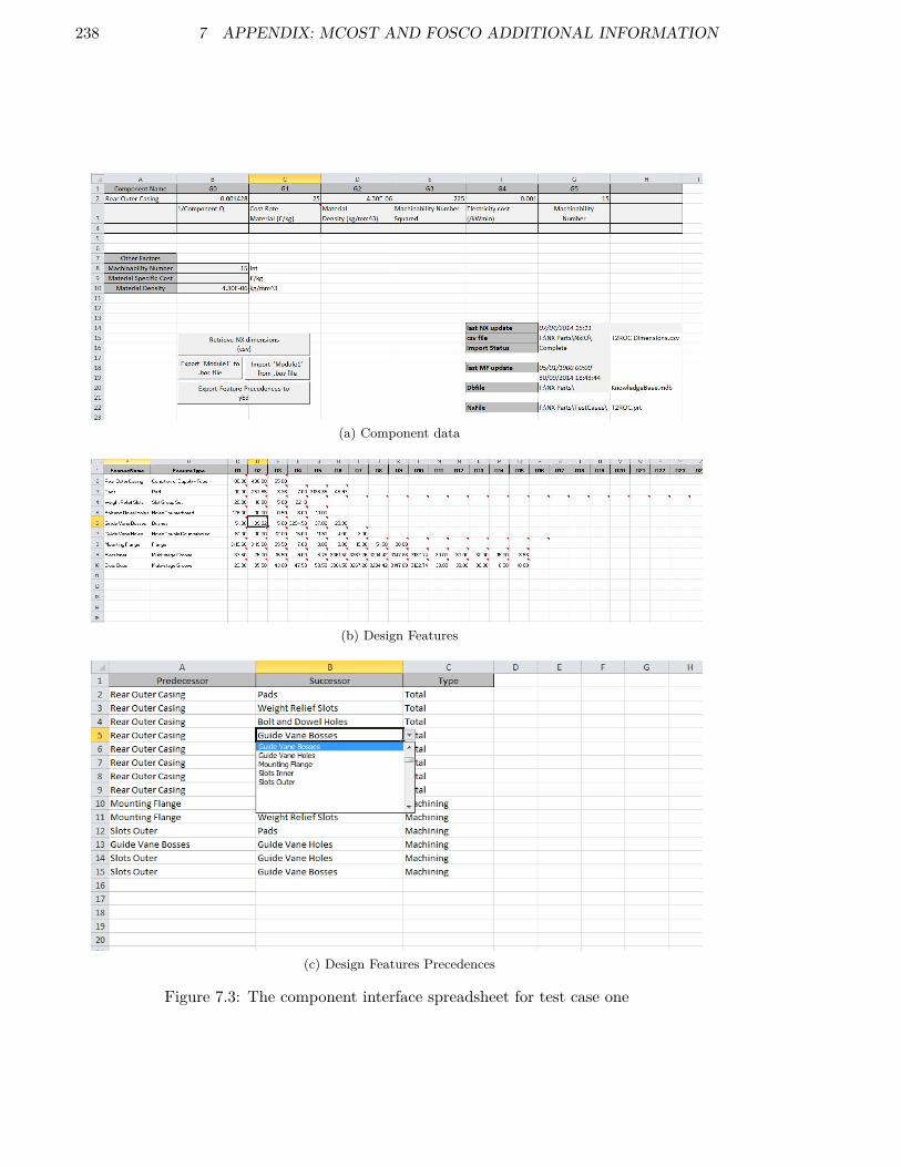
238 7 APPENDIX: MCOST AND FOSCO ADDITIONAL INFORMATION
(a) Component data
(b) Design Features
(c) Design Features Precedences
Figure 7.3: The component interface spreadsheet for test case one

7.4 Finding the convergence point 239
7.4 Finding the convergence point
Figure 7.4 shows what will occur when the combination of FMP line mesh spacing, thecone within which FMPs can be considered, and the distance from the FMP to the FSPsinteract to disqualify any FMP from the distance calculations and therefore the forcecalculations. The easiest solution is a finer mesh on the FMP lines.
Figure 7.4: An insufficient number of FMPPs

240 7 APPENDIX: MCOST AND FOSCO ADDITIONAL INFORMATION
7.5 Secondary convergence of FoSCo
The secondary convergence of FoSCo relies on a force balance, the four graphs below show(at two different scales) the force balance when the FSP is in two different positions (butthe same theta value).

7.5 Secondary convergence of FoSCo 241
(a) Full graph
(b) Close view around FSP to show the three movement vectors
Figure 7.5: When FSP is at (8,8)

242 7 APPENDIX: MCOST AND FOSCO ADDITIONAL INFORMATION
(a) Full graph
(b) Close view around FSP to show the three movement vectors
Figure 7.6: When FSP is at (7,7)

243
8 Appendix: FoSCo patent submission
This methodology, to be executed in a computer or similar device, is submitted for patentin the USA and the EU.
EU patent number 16180366.3 - 1954
US patent submission reference 5895 LMT
Note that references which are not figure references apply to the labled items on thefigures in this appendix.
8.1 Abstract
Methods of estimating a precursor shape for a part There is disclosed a method ofestimating a precursor shape (44, 45) for a part (2) suitable for manufacture via a processselected from a plurality of manufacturing processes. The method includes: generating aconvergence line (20) within the confines of a final part shape (1); providing an array (18)of spaced-apart forming shape points (19) around the final part shape (1); converging saidpoints (19) towards the convergence line (20) using a force-energy-balance technique via amovement algorithm; and applying a smoothing algorithm to the converged points (19) tocreate an estimated precursor shape (44, 45). The algorithms include coefficients specific toa predetermined one of said manufacturing processes. (To be accompanied by Figure 8.15when published).
8.2 Claims
1. A method of estimating a precursor shape (44, 45) for a part (2) suitable formanufacture via a process selected from a plurality of manufacturing processes, the methodincluding: generating a convergence line (20) within the confines of a final part shape (1);providing an array (18) of spaced-apart forming shape points (19) around the final partshape (1); converging said points (19) towards the convergence line (20) using aforce-energy-balance technique via a movement algorithm; and applying a smoothingalgorithm to the converged points (19) to create an estimated precursor shape (44, 45),wherein the algorithms include coefficients specific to a predetermined one of saidmanufacturing processes.
2. A method according to claim 1, further including selecting said predeterminedmanufacturing process from said plurality of manufacturing processes.
3. A method according to claim 1 or claim 2, further including defining said final partshape (1) prior to generation of the convergence line (20).

244 8 APPENDIX: FOSCO PATENT SUBMISSION
4. A method according to any preceding claim, wherein generation of the convergence line(20) is performed manually.
5. A method according to any one of claims 1 to 3, wherein generation of the convergenceline (20) is performed automatically.
6. A method according to any preceding claim, wherein the ends (22, 24) of saidconvergence line (20) are proximate, but spaced inwardly of the final part shape (1).
7. A method according to any preceding claim, wherein said provision of said array ofpoints (19) is one of: automated; manual; and partially automated.
8. A method according to any preceding claim, wherein each of said forming shape points(19) is assigned a respective angular value (θ) between 0° and 360°.
9. A method according to any preceding claim, wherein the angular value (θ) of eachforming shape point (19) remains constant throughout said convergence and smoothingsteps.
10. A method according to any preceding claim, wherein said final part shape (1) and saidconvergence line (20) are provided within a Cartesian coordinate system (16), such that theorigin of said coordinate system falls within the final part shape (1).
11. A method according to any preceding claim, wherein at least some of said formingshape points (19) are moved relative to respective convergence points (24) during saidconvergence and smoothing, said convergence points (24) being located at discretepositions along said convergence line (24).
12. A method according to any preceding claim, wherein some of said forming shape points(19) are moved relative to the same, shared, convergence point (24), and wherein saidshared convergence point (24) is coincident with an end (22, 23) of the convergence line(20).
13. A method according to claim 11 or claim 12, as dependent upon claim 8, wherein theconvergence point (24), relative to which each forming shape point (19) is moved duringconvergence and smoothing, is determined solely in dependence on the angular value (θ)assigned to the respective forming shape point (19).
14. A method according to any preceding claim, further including application of anadaptive grid spacing to maintain said forming shape points (19) in approximatelyequi-spaced relation to one another during said convergence and smoothing.
15. A method according to any preceding claim, wherein convergence of said forming shapepoints (19) involves a primary convergence stage followed by a secondary convergencestage, wherein said primary convergence stage is performed independently of whichever oneof said manufacturing processes is selected for manufacture of said part (2), and wherein

8.2 Claims 245
said secondary convergence stage involves application of said movement algorithm.
16. A method according to any preceding claim, wherein said movement algorithm includesa plurality of said coefficients (k1, k2, k3).
17. A method according to any preceding claim, wherein said smoothing algorithmincludes a single said coefficient (k4).
18. A method according to any preceding claim, further including the creation of said finalpart shape (1) in a CAD package.
19. A method according to claim 18, further including the creation of said convergence line(20) in said CAD package.
20. A method according to any preceding claim, wherein the method is implemented on acomputer.
21. An apparatus (47) comprising a processor (52) configured to perform the method ofany one of claims 1 to 19.
22. A computer program (54) which, when read by a computer (47), causes performance ofthe method according to any one of claims 1 to 19.
23. A non-transistory computer readable storage medium (53) comprising computerreadable instructions (54) which, when read by a computer (47), cause performance of themethod according to any one of claims 1 to 19.
24. A method of estimating a precursor shape substantially as herein described withreference to the accompanying drawings.
25. An apparatus substantially as herein described with reference to the accompanyingdrawings.
26. A computer program substantially as herein described with reference to theaccompanying drawings.
27. A non-transistory computer readable storage medium substantially as herein describedwith reference to the accompanying drawings.
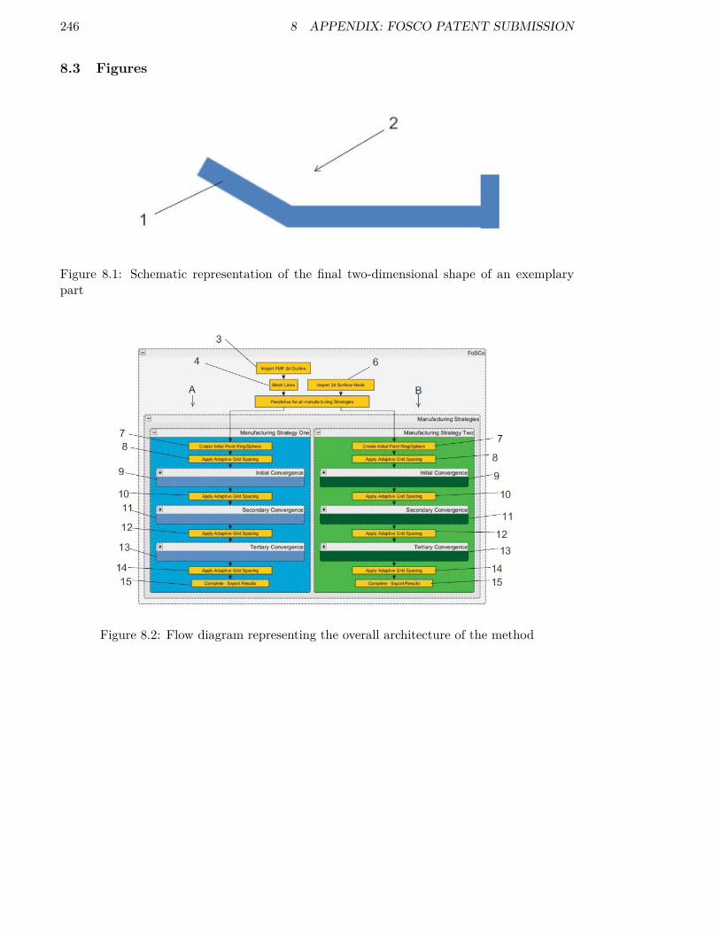
246 8 APPENDIX: FOSCO PATENT SUBMISSION
8.3 Figures
Figure 8.1: Schematic representation of the final two-dimensional shape of an exemplarypart
Figure 8.2: Flow diagram representing the overall architecture of the method
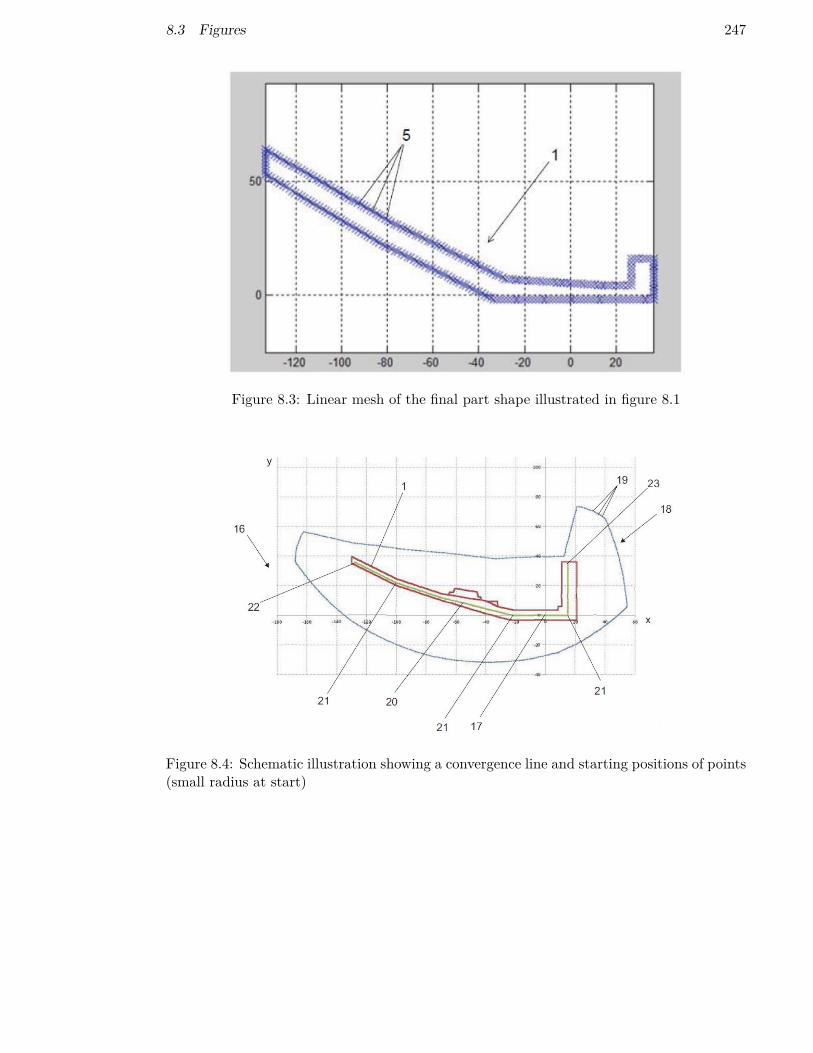
8.3 Figures 247
Figure 8.3: Linear mesh of the final part shape illustrated in figure 8.1
Figure 8.4: Schematic illustration showing a convergence line and starting positions of points(small radius at start)
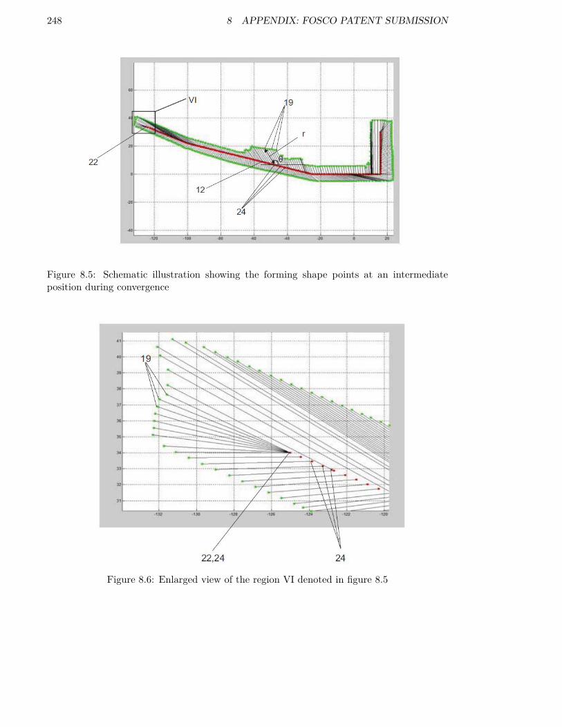
248 8 APPENDIX: FOSCO PATENT SUBMISSION
Figure 8.5: Schematic illustration showing the forming shape points at an intermediateposition during convergence
Figure 8.6: Enlarged view of the region VI denoted in figure 8.5

8.3 Figures 249
Figure 8.7: Schematic illustration showing principles involved in determining the convergencepoint
Figure 8.8: Enlarged view of the region VIII denoted in figure 8.7
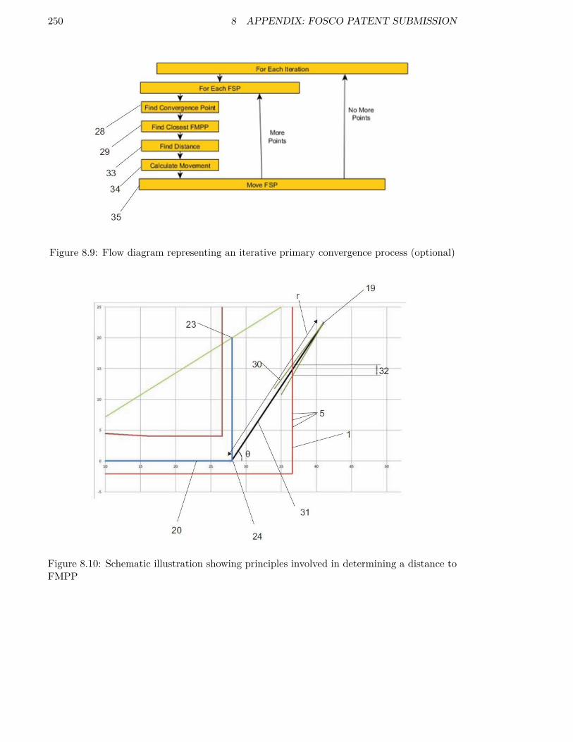
250 8 APPENDIX: FOSCO PATENT SUBMISSION
Figure 8.9: Flow diagram representing an iterative primary convergence process (optional)
Figure 8.10: Schematic illustration showing principles involved in determining a distance toFMPP
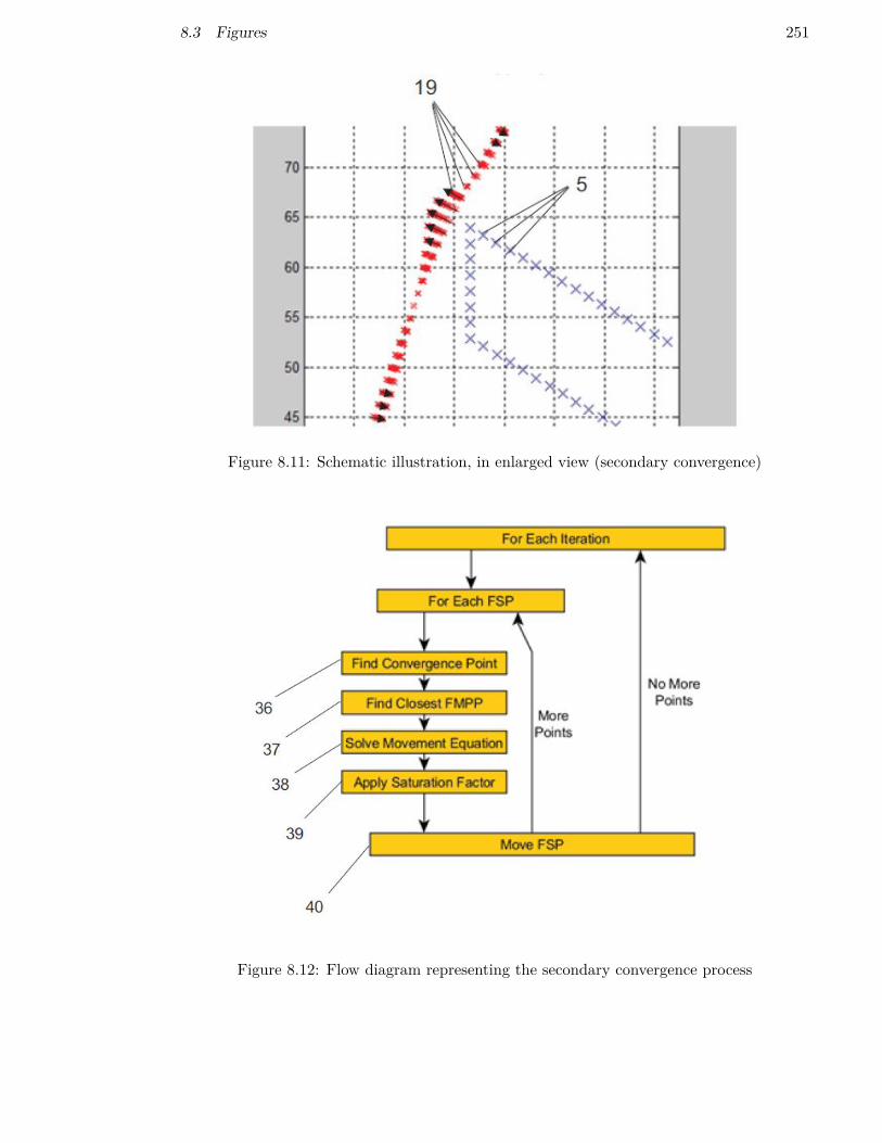
8.3 Figures 251
Figure 8.11: Schematic illustration, in enlarged view (secondary convergence)
Figure 8.12: Flow diagram representing the secondary convergence process

252 8 APPENDIX: FOSCO PATENT SUBMISSION
Figure 8.13: Flow diagram representing a tertiary convergence process
Figure 8.14: Tertiary convergence process in respect of an individual forming shape point
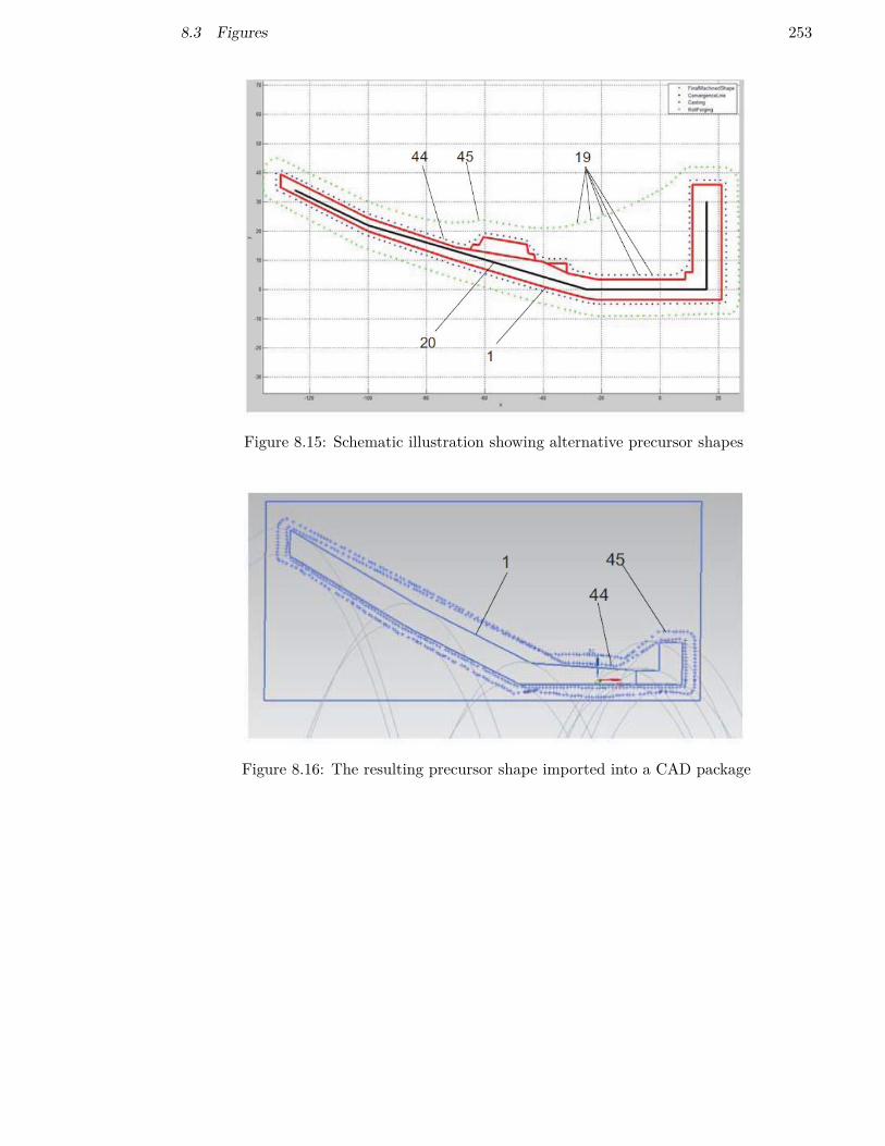
8.3 Figures 253
Figure 8.15: Schematic illustration showing alternative precursor shapes
Figure 8.16: The resulting precursor shape imported into a CAD package
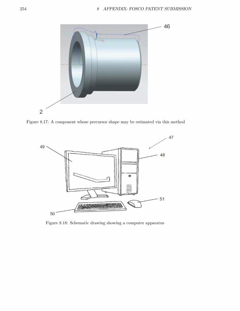
254 8 APPENDIX: FOSCO PATENT SUBMISSION
Figure 8.17: A component whose precursor shape may be estimated via this method
Figure 8.18: Schematic drawing showing a computer apparatus
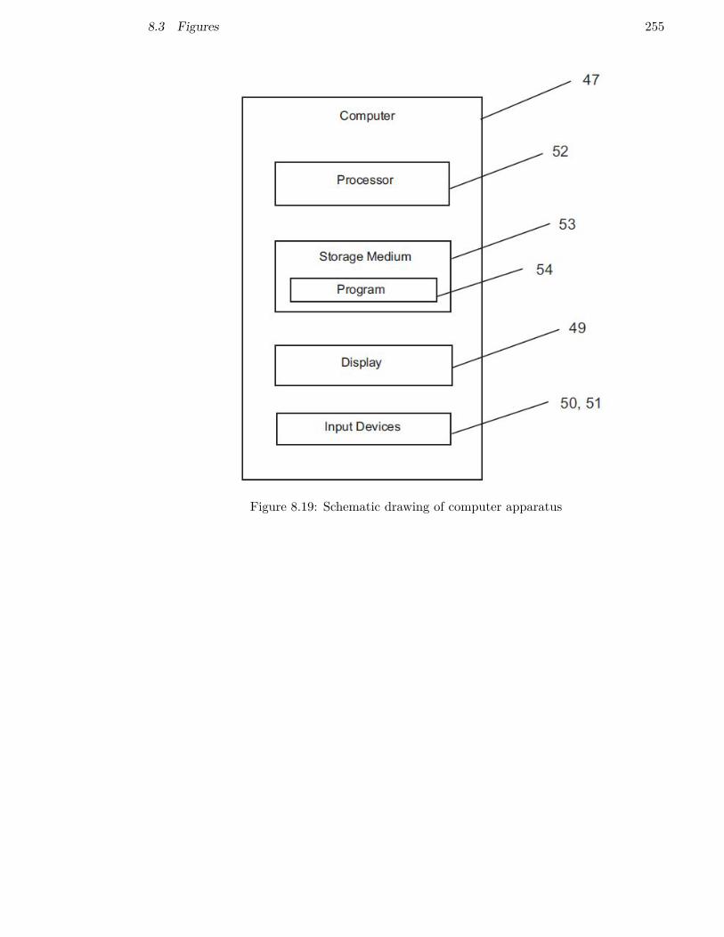
8.3 Figures 255
Figure 8.19: Schematic drawing of computer apparatus

256 8 APPENDIX: FOSCO PATENT SUBMISSION
8.4 Method
This specification relates to a method of estimating a precursor shape for a part to bemanufactured, and more particularly relates to a method of estimating a precursor shapefor a part suitable for manufacture via a process selected from a plurality of possiblemanufacturing processes.
Computer Aided Process Planning (CAPP) is a generic name for a diverse range oftechniques which can be used to take design information for parts, such as engineeringcomponents, and create therefrom an appropriate manufacturing route in the form of a setof manufacturing operations which can be used to process raw material in order to producea desired part. CAPP can be considered to represent an exercise in decision making. Thelevel of human intervention, the extent of the freedom allowed to the computer, theaccuracy of any evaluations or simulations the computer is required to run, the acceptablerun-time, and the form and extent of the information required by the computer are mattersfor the CAPP programmer and other decision makers to decide.
The manufacturing methodology used for many intricate and/or high performance partssuch as, for example, components of gas turbine engines or the like often involves theformation of a precursor volume via one of a number of possible forming manufacturingprocesses (e.g. casting and forging). The precursor part produced by the chosenmanufacturing process will often be somewhat larger than the desired final shape of thepart, and so further processing will then be required (e.g. chip forming operations) toachieve the final desired shape. As will be appreciated, the precursor shape which might beachievable by one manufacturing process will often be somewhat different to that whichmight be achievable by another manufacturing process.
As will therefore be appreciated, the manufacturing operations which are required toproduce any given part will depend on the geometry of the finished part and the shape ofthe precursor part. It is therefore useful to be able to rapidly estimate the precursor shapewhich can be created by whatever forming process (e.g. casting or forging) is to be used.In order to optimise the process and cost modelling, it is important to be able to estimatea precursor shape automatically. It has been previously proposed to estimate a precursorshape via the use of a full rule-based technique, which has been found to be accurate andto require a mid-level of computational complexity. However, this technique is not genericto all part shapes and so requires the formation of a different set of rules for each differentpart. A different set of rules is also required for each manufacturing process.
It has also been previously proposed to create a precursor shape simply by adding an offsetof a few millimetres around the final desired part shape, optionally including the use of asmoothing algorithm or taking account of sharp corners. However, these techniques areconsidered to be far from optimal.

8.4 Method 257
According to a first aspect of the present proposal, there is provided a method ofestimating a precursor shape for a part suitable for manufacture via a process selected froma plurality of manufacturing processes, the method including: generating a convergenceline within the confines of a final part shape; providing an array of spaced-apart formingshape points around the final part shape; converging said points towards the convergenceline using a force-energy-balance technique via a movement algorithm; and applying asmoothing algorithm to the converged points to create an estimated precursor shape,wherein the algorithms include coefficients specific to a predetermined one of saidmanufacturing processes.
The method may further include selecting said predetermined manufacturing process fromsaid plurality of manufacturing processes.
The method may include defining said final part shape prior to generation of theconvergence line.
Generation of the convergence line may be performed manually or automatically.
Optionally, the ends of said convergence line are proximate, but spaced inwardly of thefinal part shape.
Said provision of said array of points may be one of: automated; manual; and partiallyautomated. Each of said forming shape points may be assigned a respective angular value(θ) between 0° and 360°. Optionally, the difference between the angular values (θ) of eachneighbouring pair of points is equal.
The angular value (θ) of each forming shape point may remain constant throughout saidconvergence and smoothing steps.
Said final part shape and said convergence line may be provided within a Cartesiancoordinate system, such that the origin of said coordinate system falls within the final partshape.
Optionally, at least some of said forming shape points are moved relative to respectiveconvergence points during said convergence and smoothing, said convergence points beinglocated at discrete positions along said convergence line.
Some of said forming shape points may be moved relative to the same, shared, convergencepoint, and wherein said shared convergence point is coincident with an end of theconvergence line.
The convergence point relative to which each forming shape point is moved duringconvergence and smoothing may be determined solely in dependence on the angular value(θ) assigned to the respective forming shape point.
The method may further include application of an adaptive grid spacing to maintain said

258 8 APPENDIX: FOSCO PATENT SUBMISSION
forming shape points in approximately equi-spaced relation to one another during saidconvergence and smoothing.
Convergence of said forming shape points may involve a primary convergence stagefollowed by a secondary convergence stage, wherein said primary convergence stage isperformed independently of whichever one of said manufacturing processes is selected formanufacture of said part, and wherein said secondary convergence stage involvesapplication of said movement algorithm.
Said movement algorithm may include a plurality of said coefficients.
Said smoothing algorithm may include a single said coefficient.
The method may further include the creation of said final part shape in a CAD package.The method may also further include the creation of said convergence line in said CADpackage.
The method may be implemented on a computer.
According to a second aspect of the present proposal, there is provided an apparatuscomprising a processor configured to perform the method of the first aspect.
According to a third aspect of the present proposal, there is provided a computer programwhich, when read by a computer, causes performance of the method according to the firstaspect.
According to a fourth aspect of the present proposal, there is provided a non-transistorycomputer readable storage medium comprising computer readable instructions which, whenread by a computer, cause performance of the method according to the first aspect.
So that the proposals may be more readily understood, and so that further features thereofmay be appreciated, aspects of the proposals will now be described by way of example withreference to the accompanying drawings in which:
Figure 8.1 is a schematic representation of the final two-dimensional shape of an exemplarypart whose precursor shape may be estimated via the proposed method;
Figure 8.2 is a flow diagram representing the overall architecture of the method;
Figure 8.3 is a schematic illustration showing a linear mesh of the final part shapeillustrated in Figure 8.1, the mesh comprising a plurality of equi-spaced points identified bycrosses;
Figure 8.4 is a schematic illustration showing a convergence line provided within theconfines of the final part shape and an array of spaced-apart forming shape points arrangedaround the meshed final part shape, prior to any convergence;

8.4 Method 259
Figure 8.5 is a schematic illustration showing the forming shape points at intermediatepositions during convergence, and which shows the manner in which the points are movedtowards different positions along the convergence line;
Figure 8.6 is an enlarged view of the region VI denoted in Figure 8.5, showing in moredetail the region of an end of the convergence line; Figure 8.7 is a schematic illustrationshowing principles involved in determining the convergence point on the convergence lineto which each forming shape point will move during convergence;
Figure 8.8 is an enlarged view of the region VIII denoted in Figure 8.7, showing in moredetail the region of an end of the convergence line;
Figure 8.9 is a flow diagram representing an iterative primary convergence process whichmay be carried out on the forming shape points so that they are moved towards theconvergence line;
Figure 8.10 is a schematic illustration showing principles involved in determining a distancepertaining to the primary convergence process shown in Figure 8.9
Figure 8.11 is a schematic illustration, in enlarged view, depicting characteristics of aniterative secondary convergence process to move the forming shape points towards or awayfrom the convergence line;
Figure 8.12 is a flow diagram representing the secondary convergence process; Figure 8.13is a flow diagram representing a tertiary convergence process;
Figure 8.144 illustrates details of the tertiary convergence process in respect of anindividual forming shape point;
Figure 8.15 is a schematic illustration showing alternative precursor shapes for a part to beproduced by casting and roll forging;
Figure 8.16 shows the resulting precursor shape imported into a CAD package as a sketch;
Figure 8.17 shows a component whose two-dimensional shape may be estimated as aprecursor shape via the proposed method;
Figure 8.18 is a schematic drawing showing a computer apparatus which may be configuredto perform the method; and
Figure 8.19 is a schematic drawing showing elements of the computer apparatus illustratedin Figure 8.18.
Turning now to consider the drawings in more detail, Figure 8.1 illustrates the finalmachined part shape 1 of an exemplary part 2 whose precursor shape may be estimatedusing the method of the present proposal, as will be described in detail below. It is to be
260 8 APPENDIX: FOSCO PATENT SUBMISSION
noted that the final part shape 1 is thus the final target shape of the part 2 which is to beproduced by appropriate forming and machining processes. The particular part 2 whosefinal part shape 1 is illustrated in Figure 8.1 is shown in simplified form for reasons ofclarity but may, for example, be an annular casing component for a gas turbine engine. Itis to be noted that Figure 8.1 represents the two-dimensional final part shape 1 (in radialcross section) of the part 2. The final part shape 1 will typically be created in a ComputerAided Design (CAD) software package in a manner known per se.
Figure 8.2 illustrates schematically the overall architecture of a method in accordance withan embodiment of the present proposal. In brief outline, if the final machined part shape 1which is created in CAD is two-dimensional as illustrated in Figure 8.1, then its outline isimported into a computer program configured to implement the method, as denoted at 3 inFigure 8.2, whereupon the outline is meshed (as denoted at 4) to create a plurality ofequispaced final machined part points 5 along the outline of the final part shape 1, asshown schematically in Figure 8.3 (each final part point 5 being defined by the intersectionof a respective cross). However, it is possible instead to mesh the outline of the final partshape 2 directly within the CAD package prior to import, particularly in the case of athree dimensional surface shape, as denoted at 6 in Figure 8.2.
Following creation and/or importation of the meshed final part shape outline, the methodmay then be applied in dependence on the particular initial manufacturing process selectedto form the precursor part prior to further finishing. Figure 8.2 thus illustrates abifurcation in the process flow into two possible alternative branches A, B, each of which isrepresentative of the method pertaining to a respective manufacturing process. Forexample, branch A could be considered to represent the method applicable to estimate aprecursor shape for a forging process, whilst branch B could be considered to represent themethod applicable to create a precursor shape for a casting process. It is to be noted,however, that more than two manufacturing processes could be provided for. It is also tobe noted that the subsequent method steps within each branch A, B of the method aregenerally identical in many respects, and are based on use of the same processes,techniques and algorithms, regardless of which manufacturing process is to be used. As willbe described in more detail, however, the implementation of the method will be based ondifferent parameters depending on which manufacturing process is to be used, whilst thealgorithms use by the method will remain the same for all possible manufacturing processes.
Branches A and B thus each comprise a series of stages and processes, some of which areoptional as will be described in more detail hereinafter, namely:
• the creation of an array of spaced-apart forming shape points around the meshedfinal part shape outline, as denoted at 7;
• the application of adaptive grid spacing to the array of forming shape points in orderto ensure an even distribution of the points, as denoted at 8;
8.4 Method 261
• primary convergence of the forming shape points, performed in an iterative manner,generally towards the final part shape 1, as denoted at 9,
• further application of adaptive grid spacing to the converged forming shape points toensure even distribution, as denoted at 10;
• secondary convergence of the forming shape points, performed in an iterative manner,generally towards the final part shape 1, as denoted at 11;
• further application of adaptive grid spacing to the converged forming shape points toensure even distribution, as denoted at 12;
• tertiary convergence, involving the use of a smoothing algorithm and again performedin an iterative manner , as denoted at 13;
• further application of adaptive grid spacing to the converged forming shape points, asdenoted at 14; and
• export of the resulting precursor shape to a CAD package, as denoted at 15, forsubsequent automatic creation of reference dimensions to inform a CAPP system howmuch machining will be necessary to achieve the final part shape 1.
Turning now to consider Figure 8.4, the meshed final part shape 1 (illustrated in moredetail than in Figure 8.3) is shown in a native Cartesian coordinate system 16 comprising ahorizontal x-axis and a vertical y-axis. The final part shape 1 is located over the origin 17of the coordinate system. An array 18 of spaced-apart forming shape points 19 is thencreated around the meshed final part shape 1. In Figure 8.4, each forming shape point 19 isdenoted by a respective cross, the crosses for each respective point 19 being arranged in aclosed contour around and entirely encompassing the meshed final part shape 1 in spacedrelation thereto. The forming shape points 19 are thus distributed in the native coordinatesystem, such that each individual point 19 will have a respective unique (x, y) locationwithin the coordinate system. As will be appreciated, there are a very large number offorming shape points 19 provided in this manner, such that the resolution of Figure 8.4makes it appear that their crosses coalesce to form a thick line. The particular shape of theclosed contour array will depend (indirectly) on the final part shape 1, as will be describedin more detail hereinafter. It is also to be noted that Figure 8.4 depicts the forming shapepoints 19 in respective starting positions that are considerably closer to the final partshape 1 than would actually be the case in practice, for illustrative purposes. The mannerin which the actual starting positions of the forming shape points 19 are determined, andthus also the shape of the initial array 18, will become apparent hereinafter.
As will also be explained in more detail below, the method involves iterative convergence ofthe forming shape points 19, generally towards the final part shape 1, such that uponcompletion of the convergence process the locations of the forming shape points 19 willcollectively define the outline of a precursor shape for the part which is to be produced. As

262 8 APPENDIX: FOSCO PATENT SUBMISSION
already indicated above, convergence of the forming shape points 19 may involve a numberof discrete stages. For example, in the embodiment of the method illustrated schematicallyin Figure 8.2, the overall convergence process may involve primary convergence, followedby secondary convergence, which is then followed by tertiary convergence via a smoothingalgorithm. However, an important aspect of the method is that the forming shape points19 do not all converge towards the same convergence point. It is this aspect of the methodwhich allows the precursor shape created to be as close as possible to the final part shape 1in a near net shape manufacturing process.
The method therefore also involves the creation of a convergence line relative to which theforming shape points 19 will each be converged. An exemplary convergence line 20 isillustrated in Figure 8.4. It is to be noted that the convergence line 20 is entirely envelopedby the final part shape 1. The convergence line 20 may thus include a number of bends orcorners 21 to ensure that it remains within the final part shape 1 at all points along itslength.
It may alternatively be possible for the convergence line 20 to be curved. The ends 22, 23of the convergence line 20 should not be too close to each other relative to the origin 17 ofthe coordinate system 16.
Returning now to consider the forming shape points 19, each point will be assigned arespective and unique fixed angular theta value (θ) of between 0° and 360°, as measuredcounter-clockwise from a notional horizontal line parallel to the x-axis of the coordinatesystem 16. For illustrative purposes, an example may be considered in which the closedcontour array 18 comprises one-hundred forming shape points 19 (although in practice it isenvisaged that many more forming shape points will be used for reasons of accuracy). Insuch an example: the first forming shape point 19 would thus be assigned a theta valuecalculated as 1 x (360/100), so θ1 = 3.6°; the second forming shape point 19 would beassigned a theta value calculated as 2 x (360/100), so θ2 = 7.2°; the third forming shapepoint would be assigned a theta value as 3 x (360/100), so θ3 = 10.8°; and so on. Theangular difference between the theta values of each neighbouring pair of forming shapepoints 19 will thus be equal throughout the full 360° of the closed contour array 18.
As indicated above, convergence of the forming shape points 19 will involve movement ofthe points relative to the convergence line 20. In this regard, it is to be noted that many ofthe points 19 will be moved relative to respective and unique convergence points along theconvergence line 20, although it is possible that some of the points 19 around the ends 22,23 of the convergence line 20 will all need to be moved relative to the same end point. Thisprinciple can be seen in Figure 8.5 which illustrates the forming shape points 19 at a pointin time which is part-way through the convergence process. In more detail, each formingshape point is shown connected to its convergence point 24 on the convergence line 20 by anotional line having a length r measured from the respective convergence point 24, andwhich makes an angle θ relative to a horizontal line through the convergence point 24,

8.4 Method 263
where θ is the fixed theta value assigned to the respective forming shape point 19. Theposition of each forming shape point 19 relative to its convergence point 24 may thus bedefined by polar coordinates (r, θ). During convergence, as will be explained in more detailbelow, the theta value θ of each forming shape point 19 will remain fixed, but the point’s rvalue will change, such that each forming shape point 19 will be moved along itsaforementioned notional line. Figure 8.6 illustrates the region of the end point 22 of theconvergence line 20 shown in Figure 8.6 in more detail, and in particular illustrates howseveral of the forming shape points 19 around the end of the convergence line will all beconverged relative to the same convergence point 24 (coincident with the end of theconvergence line 20) despite evertheless still having different fixed theta values.
As will be appreciated, it is therefore necessary to define a convergence point 24 on theconvergence line 20 for each forming shape point 19. In this regard, it is to be noted thatthe location along the convergence line 20 of the convergence point 24 for any givenforming shape point 19 will depend solely on the theta value (θ) assigned to that formingshape point. The process by which this is done will now be described below in more detail.
When the convergence line 20 is constructed, its end points 22, 23 are each assigned a rangeof angular values, based on respective lines extending from the origin 17 of the coordinatesystem 16 and passing through each end point 22, 23 as illustrated in figures 7 and 8, ofplus and minus 3°. In figures 7 and 8, the extent of these angular values at each end 22, 23of the convergence line 20 are denoted by respective pairs of boundary lines 26, 27. Theinterbound arc angle between the boundary lines 26, 27 of each pair will thus be 6°.
Any forming shape point 19 falling between either pair of boundary lines 26, 27 will beconverged relative to a convergence point 24 coincident with the respective end point 22, 23of the convergence line 20.
So, taking the example illustrated in figures 7 and 8, it will be noted that the first endpoint 22 of the convergence line 20 has Cartesian coordinates of (-130, 60), whilst thesecond end point has coordinates of (28, 20). The angles from each of these end points, asmeasured from the positive x-axis of the coordinate system 16 can thus be calculated viatrigonometry to be 155.2249° and 35.5378° respectively. Thus, any forming shape pointswhich have a theta value (θ) of 155.2249 ± 3 will take the first end point 22 as their(shared) convergence point, whilst any forming shape points 19 which have a theta value(θ) of 35.5378 ± 3 will take the second end point 23 as their (shared) convergence point.
All of the other forming shape points 19 will lie between one of the boundary lines 26 at thefirst end 22 of the convergence line 20 and one of the boundary lines 27 at the second end23 of the convergence line, and their convergence points 24 are determined in dependenceon how far between the boundary lines, in an angular sense, the forming shape points 19 lie.
Having regard to Figure 8.7, the upper boundary line 27 of the start-point (“sp”) end 23 ofthe convergence line has an angle denoted spmax which in this specific example will be
264 8 APPENDIX: FOSCO PATENT SUBMISSION
35.5378+3 = 38.5378. Similarly, the upper boundary line 26 at the end-point (“ep”) 22 ofthe convergence line 20 has an angle denoted epmin which in this specific example will be155.2249-3 = 152.2249.
So for forming shape points located generally above the convergence line 20 shown inFigure 8.7, or more accurately between spmax and epmin , the position of their respectiveconvergence points 24, as measured along the convergence line 20 from the start-point end23, may be expressed as a percentage of the total length of the convergence line 20 by theexpression:
100 · ((θ − spmax) /AIB) (8.1)
Where AIB is the interbound arc angle: (i.e. epmin-spmax or(155.2249-3)-(35.5378+3)=113.6871 degrees in the specific example illustrated).
So, taking an example of a forming shape point 19 having a theta value (θ) of 45°, and thespecific convergence line 20 illustrated in Figure 8.7 and thus having the above statedspmax and epmin values, then this expression will give a percentage value of 5.68%, suchthat the forming shape point’s convergence point 24 will be located at a position on theconvergence line 20 and 5.68% of the total length of the convergence line 20 along the linefrom the start point 23 of the line.
The same principle may be used to identify which of the convergence points 24 should beused for those forming shape points 19 which are located generally below the convergenceline shown in Figure 8.7, or more accurately between the lower boundary line 27 of theendpoint 23 (having an angle denoted epmax.) and the lower boundary line 26 of thestart-point 22 (having an angle denoted spmin ). So for forming shape points locatedgenerally below the convergence line 20 shown in Figure 8.7, or more accurately betweenspmin and epmsx, the position of their respective convergence points 24, as measured alongthe convergence line 20 from the start-point end 23, may be expressed as a percentage ofthe total length of the convergence line 20 by the expression:
100 · ((θ − epmax) /AIB) (8.2)
Where AIB in this specific example = 32.5378 +360 - 158.2249 = 234.3129.
When the converging point 24 for each forming shape point 19 is known (as calculatedabove from the respective theta value of each point 19) then the initial array 18 of formingshape points 19 can be created around the convergence line 20. The forming shape pointsare positioned relative to their respective convergence points 24 in dependence on theirpolar coordinates (r, θ), where r is the same for each forming shape point 19.
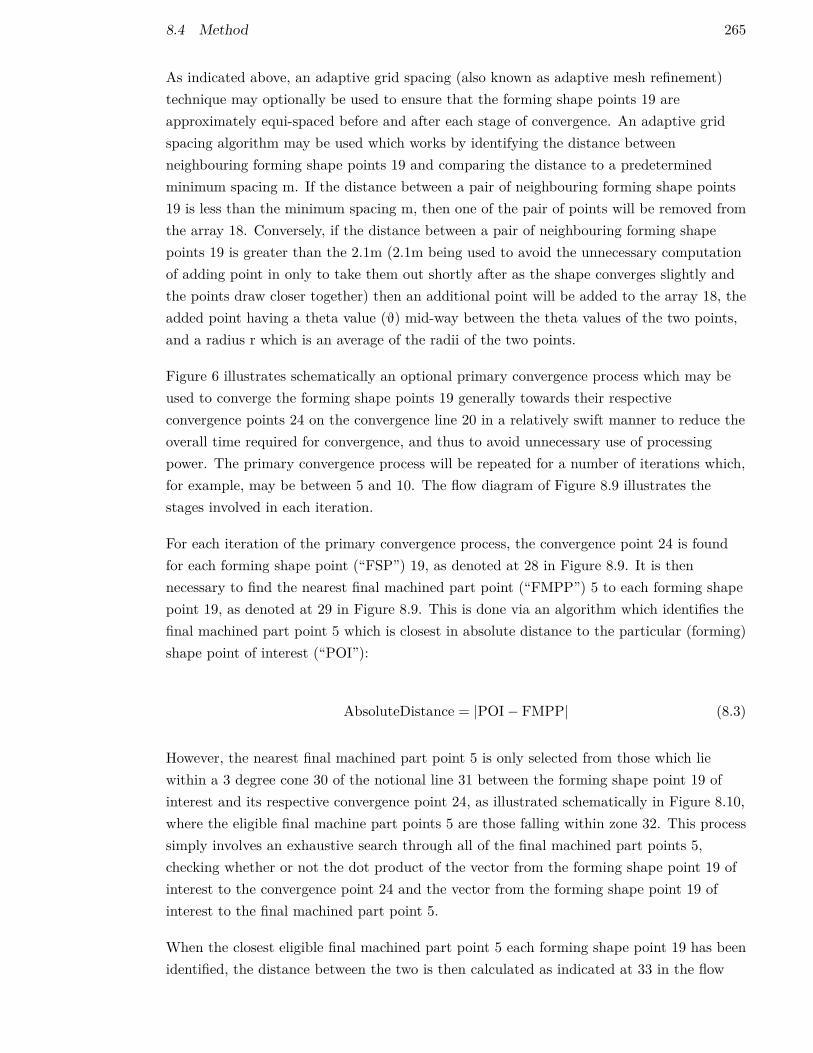
8.4 Method 265
As indicated above, an adaptive grid spacing (also known as adaptive mesh refinement)technique may optionally be used to ensure that the forming shape points 19 areapproximately equi-spaced before and after each stage of convergence. An adaptive gridspacing algorithm may be used which works by identifying the distance betweenneighbouring forming shape points 19 and comparing the distance to a predeterminedminimum spacing m. If the distance between a pair of neighbouring forming shape points19 is less than the minimum spacing m, then one of the pair of points will be removed fromthe array 18. Conversely, if the distance between a pair of neighbouring forming shapepoints 19 is greater than the 2.1m (2.1m being used to avoid the unnecessary computationof adding point in only to take them out shortly after as the shape converges slightly andthe points draw closer together) then an additional point will be added to the array 18, theadded point having a theta value (θ) mid-way between the theta values of the two points,and a radius r which is an average of the radii of the two points.
Figure 6 illustrates schematically an optional primary convergence process which may beused to converge the forming shape points 19 generally towards their respectiveconvergence points 24 on the convergence line 20 in a relatively swift manner to reduce theoverall time required for convergence, and thus to avoid unnecessary use of processingpower. The primary convergence process will be repeated for a number of iterations which,for example, may be between 5 and 10. The flow diagram of Figure 8.9 illustrates thestages involved in each iteration.
For each iteration of the primary convergence process, the convergence point 24 is foundfor each forming shape point (“FSP”) 19, as denoted at 28 in Figure 8.9. It is thennecessary to find the nearest final machined part point (“FMPP”) 5 to each forming shapepoint 19, as denoted at 29 in Figure 8.9. This is done via an algorithm which identifies thefinal machined part point 5 which is closest in absolute distance to the particular (forming)shape point of interest (“POI”):
AbsoluteDistance = |POI− FMPP| (8.3)
However, the nearest final machined part point 5 is only selected from those which liewithin a 3 degree cone 30 of the notional line 31 between the forming shape point 19 ofinterest and its respective convergence point 24, as illustrated schematically in Figure 8.10,where the eligible final machine part points 5 are those falling within zone 32. This processsimply involves an exhaustive search through all of the final machined part points 5,checking whether or not the dot product of the vector from the forming shape point 19 ofinterest to the convergence point 24 and the vector from the forming shape point 19 ofinterest to the final machined part point 5.
When the closest eligible final machined part point 5 each forming shape point 19 has beenidentified, the distance between the two is then calculated as indicated at 33 in the flow

266 8 APPENDIX: FOSCO PATENT SUBMISSION
diagram of Figure 8.9. The distance which each forming shape point 19 should then bemoved towards its convergence point 24, along its notional line 31 is then calculated, beingten units less than the linear distance between the forming shape point 19 and its nearesteligible final machined part point 5, as indicated at 34 in Figure 8.9. The forming shapepoints 19 are then moved accordingly, as indicated at 35 in Figure 8.9 to complete theiteration. It is to be noted in this regard that whilst the distance moved by each formingshape point 19 is calculated on the basis of its distance from its nearest eligible finalmachined part point 5, each forming shape point 19 is actually moved along its notionalline 31. In the example used, the distance moved by each forming shape point 19 is set atten units less than the distance between the respective forming shape point 19 and itsnearest eligible final machined part point 5 so that even a very course mesh of the finalmachined part points 5 (for example less than 20 units) will not allow the forming shapepoint 19 to move past the meshed final part shape 1. It is to be appreciated that careshould be exercised when defining the actual proportion of the distance between eachforming shape part 19 and its nearest final machined part point 5 which is used formovement of the forming shape points 19, on the basis of the intended size of the finalmachined part. The example of ten units given is intended to be representative of asuitable degree of movement appropriate to estimate the precursor shape of a moderatelysized gas turbine component such as the annular casing component illustrated, but a largerdegree of movement may be appropriate for larger components.
Primary convergence is continued in the manner described above and illustrated in Figure8.9 until the forming shape points 19 stop moving.
Following primary convergence of the forming shape points 19 as explained above for anappropriate number of iterations, the forming shape points 19 are then moved further via asecondary convergence process, as depicted in the flow diagram of Figure 8.12. Thesecondary convergence process is performed for a considerably larger number of iterationsthat the primary convergence process and typically for between 500 and 1000 iterations.
Conceptually, the secondary convergence process represents a balance between convergenceforces and inverse squared repulsion from each forming shape point’s nearest eligible finalmachined part point 5 (determined in the same manner as described above). Each point 19is thus drawn along its respective notional lines 31, relative to its respective convergencepoint 24 according to:
• A force (F1) pulling the point 19 towards its convergence point 24;
• A force (F2) pulling the point 19 towards its nearest eligible final machined partpoint 5; and
• An inverse squared force (F3) pushing it away from its nearest eligible final machinedpart point 5.

8.4 Method 267
Having regard to Figure 8.11, it will thus be noted that this characteristic of the secondaryconvergence process serves to pull the forming shape points 19 which are relatively distantto their nearest eligible final machined part points 5 inwardly towards the convergence line20, whilst pushing the forming shape points 19 which are relatively close to their nearesteligible final machined part points 5 outwardly and away from the convergence line 20, asindicated schematically by the arrows in Figure 8.11.
For each iteration of the secondary convergence process, the convergence point 24 is foundfor each forming shape point (“FSP”) 19, as denoted at 36 in Figure 8.12. It is then againnecessary to find the nearest eligible final machined part point (“FMPP”) 5 to eachforming shape point 19, as denoted at 37 in Figure 8.12, and this is achieved in the samemanner as described above in connection with the primary convergence process. Themovement of each forming shape point 19 will then be determined via a movementalgorithm, as denoted at 38 in Figure 8.12, and the application of a saturation factor, asdenoted at 39, as will be described in more detail below.
Where n denotes a unit vector from a forming shape point 19 towards its convergencepoint 24, L denotes the location of the forming shape point 19 in the Cartesian coordinatesystem 16, Mp denotes the position of the nearest eligible final shape point 5, and Cpdenotes the location of the convergence point 24, then it follows that:
CP =
xc
yc
0
(8.4)
Cp represents the co-ordinates of the convergence point 24
L = cp + r
sin (θ)cos (θ)
0
(8.5)
L represents the Cartesian location of the forming shape point 19
n = r
sin (θ)cos (θ)
0
(8.6)
n represents the vector from the forming shape point 19
n̂ = n
|n|(8.7)
268 8 APPENDIX: FOSCO PATENT SUBMISSION
The unit vector of nB = L−Mp (8.8)
B represents the vector from the final machined part point 5 to the forming shape point 19
B̂ = B
|B|(8.9)
The unit vector of B.
The forces F1 , F2 , and F3 mentioned above may be expressed thus:
F1 = k1 · n̂ (8.10)
F2 = k2 · B̂ (8.11)
F3 = k3 ·B̂
|B|2(8.12)
Where k1, k2, and k3 is are empirically derived coefficients whose values will depend onwhich particular manufacturing process is to be used for production of the part, and thusfor which manufacturing process the precursor shape is to be estimated. It will therefore benoted that the values for k1, k2, and k3 will be different for a casting process than for a rollforging process for example.
So:
F =3∑
n=1Fn (8.13)
The required distance m by which each forming shape point must be moved along itsnotional line 31 may thus be expressed as:
m = F · n̂ (8.14)
And so each forming shape point 19 is thus moved accordingly, as denoted at 40 in Figure8.12. The secondary convergence process is repeated iteratively until the forming shapepoints 19 stop moving with each iteration.
Some exemplary values for the coefficients k1, k2, and k3 for casting, die forging and rollforging are set out in the table below:
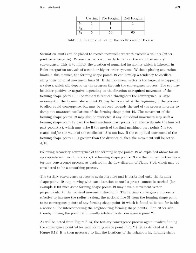
8.4 Method 269
Casting Die Forging Roll Forgingk1 1 1 1k2 1 1 1k3 5 50 60
Table 8.1: Example values for the coefficients for FoSCo
Saturation limits can be placed to reduce movement where it exceeds a value x (eitherpositive or negative). Where x is reduced linearly to zero at the end of secondaryconvergence. This is to inhibit the creation of numerical instability which is inherent inEuler integration analysis of second or higher order systems. Without placing saturationlimits in this manner, the forming shape points 19 can develop a tendency to oscillatealong their notional movement lines 31. If the movement vector is too large, it is capped ata value x which will depend on the progress through the convergence process. The cap maybe either positive or negative depending on the direction or required movement of theforming shape point 19. The value x is reduced throughout the convergence. A largemovement of the forming shape point 19 may be tolerated at the beginning of the processto allow rapid convergence, but may be reduced towards the end of the process in order todamp out unwanted oscillations of the forming shape point 19. The movement of theforming shape points 19 may also be restricted if any individual movement may shift aforming shape point 19 past the final machined part points (i.e. effectively into the finishedpart geometry), which may arise if the mesh of the final machined part points 5 is toocoarse and/or the value of the coefficient k3 is too low. If the computed movement of theforming shape point 19 is greater than the distance d, then the movement will be set tod/10.
Following secondary convergence of the forming shape points 19 as explained above for anappropriate number of iterations, the forming shape points 19 are then moved further via atertiary convergence process, as depicted in the flow diagram of Figure 8.14, which may beconsidered to be a smoothing process.
The tertiary convergence process is again iterative and is performed until the formingshape points 19 stop moving with each iteration or until a preset counter is reached (forexample 1000 since some forming shape points 19 may have a movement vectorperpendicular to the required movement direction). The tertiary convergence process iseffective to increase the radius r (along the notional line 31 from the forming shape pointto its convergence point) of any forming shape point 19 which is found to lie too far insidea notional line interconnecting the neighbouring forming shape points 19 on either side,thereby moving the point 19 outwardly relative to its convergence point 24.
As will be noted from Figure 8.13, the tertiary convergence process again involves findingthe convergence point 24 for each forming shape point (“FSP”) 19, as denoted at 41 inFigure 8.13. It is then necessary to find the locations of the neighbouring forming shape

270 8 APPENDIX: FOSCO PATENT SUBMISSION
points 19 to each side of the forming shape point 19 of interest, as denoted at 42 in Figure8.13, after which a smoothing algorithm is solved for the point, as denoted at 43, in orderto determine whether or not the point should be moved outwardly from its convergencepoint 24.
The manner in which this is achieved may be understood having regard to Figure 8.14, inwhich the forming shape point 19 of interest is denoted as P, and the two neighbouringforming shape points 19 to each side of the point of interest are denoted A and Brespectively. The vector between the two neighbouring points A and B is found and a lineAB is drawn between the two neighbouring points. The shortest vector, denoted by PI inFigure 8.14, between the forming shape point of interest P and the line AB is thencalculated. The allowable magnitude (M) of vector PI is defined by:
M = k4 · |AB| (8.15)
Where k4 is an empirically derived coefficient whose value will depend on which particularmanufacturing process is to be used for production of the part, and thus for whichmanufacturing process the precursor shape is to be estimated. By way of example k4
equals,
• 1 for a casting process;
• 0.005 for a die forging process;
• 0.005 for a roll forging process.
Vector CP shown in Figure 8.14 denotes a vector from the forming shape point’sconvergence point 24 to the forming shape point itself. If the dot product of vector PI andvector CP is negative, then the forming shape point of interest P will lie within the line ABrelative to its convergence point 24. If this is the case, and if the magnitude of vector PI isgreater than the allowable amount M, as calculated above, then the forming shape point Pwill be moved outwardly, further away from its convergence point 24, along its positionvector until PI no longer exceeds M. In this regard, it is proposed to move the formingshape point outwardly by a distance equal to 0.999M - PI . This expression ensures that,when used iteratively the point P will lie just inside the acceptable region, provided thatthe movement vector is not perpendicular to the required direction of travel.
Tertiary convergence (smoothing) continues as explained above, in an iterative manner,until there is no longer any movement of the forming shape points 19. At this point, theforming shape points 19 will collectively define the outline of an approximately optimisedprecursor shape which can be produced by the chosen manufacturing process, and whichwill require minimum subsequent machining to achieve the final part shape 1. Figure 8.15illustrates exemplary precursor shapes achieved via the method explained above for casting
8.4 Method 271
and for roll-forging, relative to the final part shape 1 and the convergence line 20. Outlineshape 44 represents an exemplary precursor shape for casting, and outline shape 45represents an exemplary precursor shape for roll-forging. As will be noted, the precursorshape 44 for casting is considerably closer to the final part shape 1 than is the precursorshape 45 for rollforging.
Following estimation of the precursor shapes 44, 45 via the method described above, theprecursor shapes will then be imported back into the CAD package which was originallyused to create the final part shape 1, as illustrated in Figure 8.16. The CAD package canthen be used to calculate the dimensions of the precursor shapes 44, 45 automatically, sothat the dimensions can then be used in the chosen production process to achieve theprecursor shape.
Figure 7 illustrates an exemplary part 2, whose 2-dimensional precursor shape 46 may beestimated via the method described above. It is to be appreciated that whilst the methodhas been described above with specific reference to the estimation of a 2-dimensionalprecursor shape, the method can also be used to estimate a 3-dimensional precursor shape.
As will be appreciated, the above-described method is suitable for implementation on acomputer.
Figure 18 illustrates an exemplary computer apparatus 47 which may be configured toimplement and run the above-described method. The computer apparatus illustrated isshown in the form of a conventional desktop computer, and thus comprises a system unit48 to which are connected a display unit 49, and input devices in the form of a keyboard 50and a mouse 51. Having regard to Figure 8.19, the computer apparatus 47 may compriseone or more processors 52 configured to perform the above-described method. Thecomputer apparatus 47 may also comprise, or be configured to receive, a storage medium53. The storage medium is a non-transistory computer readable storage medium which cantake any convenient form, but which excludes merely transistory or propagating signals.The storage medium 53 contains computer readable instructions in the form of a computerprogram 54 which, when read by the computer 47 via its processor 52, cause performanceof the above described method.
When used in this specification and claims, the terms “comprises” and “comprising” andvariations thereof mean that the specified features, steps or integers are included. Theterms are not to be interpreted to exclude the presence of other features, steps or integers.
The features disclosed in the foregoing description, or in the following claims, or in theaccompanying drawings, expressed in their specific forms or in terms of a means forperforming the disclosed function, or a method or process for obtaining the disclosedresults, as appropriate, may, separately, or in any combination of such features, be utilisedfor realising the invention in diverse forms thereof.

272 8 APPENDIX: FOSCO PATENT SUBMISSION
While the invention has been described in conjunction with the exemplary embodimentsdescribed above, many equivalent modifications and variations will be apparent to thoseskilled in the art when given this disclosure. Accordingly, the exemplary embodiments ofthe invention set forth above are considered to be illustrative and not limiting. Variouschanges to the described embodiments may be made without departing from the spirit andscope of the invention.


![arXiv:1912.05704v1 [astro-ph.HE] 12 Dec 2019 - ePrints Soton](https://static.fdokumen.com/doc/165x107/631962ea1a1adcf65a0ea184/arxiv191205704v1-astro-phhe-12-dec-2019-eprints-soton.jpg)


