Multispecies Dynamics in Weakly IonizedDusty Protoplanetary Disks

Leonardo Krapp

Supervisors:

Oliver Gressel, Pablo Benítez-Llambay and Martin E. Pessah

PhD Thesis in Theoretical and Computational Astrophysics

The Niels Bohr Institute

This thesis has been submitted to the PhD School of The Faculty of Science, University of Copenhagen

Multispecies Dynamics in Weakly Ionized Dusty Protoplanetary Disks

PhD Thesis in Theoretical and Computational Astrophysics

Krapp Leonardo

Supervisors:

Oliver Gressel, Pablo Benítez-Llambay and Martin E. Pessah.

The Niels Bohr International Academy

The Niels Bohr Institute

Faculty of Science

University of Copenhagen

July 8, 2019

i

Abstract

Understanding the dynamical evolution of protoplanetary disks is of vital importance in modern

astrophysics because many of these environments are deemed to evolve into planetary systems like

our own. In recent years, ALMA observations of the dust component and CO emission unveiled the

presence of substructures such as spiral arms, rings, and gaps, and indicated that protoplanetary disks

have a very rich dynamical activity. However, it is not clear yet whether the observed features are

signatures of planets in formation, given the complexity of the astrophysical processes taking place at

each of the different disk scales.

In this thesis, we focus our efforts on studying the momentum transfer between different species and its

effect on the disks evolution. Despite disks being poorly ionized, charged species can transfer energy

and momentum from the magnetic field to the neutrals due to collisions, significantly affecting the

dynamics. In addition, the aerodynamical coupling between dust particles and the gaseous component

has significant consequences for the dust dynamics and evolution. Thus, collisions play an important

role in affecting different processes related to accretion mechanisms, the growth of dust particles, and

the planetesimal formation. We base our discussion on three publications that define the core of this

research. We first introduce a framework to solve the momentum exchange between multiple species

with particular emphasis on dust dynamics. We then use this framework to study the impact of the

self-organization induced by the Hall effect on the dust evolution, and the linear and non-linear phase

of the streaming instability.

More specifically, we present an asymptotically and unconditionally stable numerical method to account

for the momentum transfer between multiple species. We show that the scheme conserves momentum

to machine precision and that its implementation in the publicly available code FARGO3D converges

to the correct equilibrium solution. Aiming at studying dust dynamics, we use the implementation to

address problems such as damping, damped sound waves, local and global gas-dust radial drift in a disk

and linear streaming instability. We furthermore provide analytical or exact solutions to each of these

problems considering an arbitrary number of species. We successfully validate our implementation by

recovering the solutions from the different test problems to second- and first-order accuracy in space

and time, respectively. From this, we conclude that our scheme is suitable, and very robust, to study the

self-consistent dynamics of several fluids.

In the field of non-ideal magnetohydrodynamics, we investigate the evolution of turbulence triggered

by the magneto-rotational instability, including the Hall effect and considering vertically unstratified

ii

cylindrical disk models. In the regime of a dominant Hall effect, we robustly obtain large-scale self-

organized concentrations in the vertical magnetic field that remain stable for hundreds of orbits. For

disks with initially only vertical net flux alone, we confirm the presence of zonal flows and vortices that

introduce regions of super-Keplerian gas flow. Including a moderately strong net-azimuthal magnetic

flux can significantly alter the dynamics, partially preventing the self-organization of zonal flows.

For plasma beta-parameters smaller than 50, large-scale, near-axisymmetric structures develop in

the vertical magnetic flux. In all cases, we demonstrate that the emerging features are capable of

accumulating dust grains for a range of Stokes numbers.

Finally, we study the linear and non-linear phase of the streaming instability. This instability is

thought to play a central role in the early stages of planet formation by enabling the efficient bypass

of several barriers hindering the formation of planetesimals. We recover linear and non-linear results

from previous works considering only one-dust species, validating our developed framework to study

dust dynamics. Treating dust as a pressureless fluid, we run non-linear shearing-box simulations of

the streaming instability and compare our results with two different setups previously obtained with

Lagrangian particles. Simulations with Stokes number of unity show an excellent agreement with

those performed with particles. However, in the other test case, which has a ten times smaller Stokes

number, convergence with resolution is not found. We conclude that further studies are required in

other to address whether the pressureless fluid approach is suitable for studying the non-linear phase of

the streaming instability. We furthermore present the first study exploring the efficiency of the linear

streaming instability when a particle-size distribution is considered. We find that, for a given dust-to-gas

mass ratio, the multi-species streaming instability grows on timescales much longer than those expected

when only one dust species is involved. In particular, distributions that contain dust-to-gas density

ratios close to unity lead to unstable modes that can grow on timescales comparable to, or larger

than those of secular instabilities. We anticipate that processes leading to particle segregation and/or

concentration can create favorable conditions for the instability to grow fast. Our findings may have

important implications for a large number of processes in protoplanetary disks that rely on the streaming

instability as usually envisioned for a unique dust species. Our results suggest that the growth rates of

other resonant-drag-instabilities may also decrease considerably when multiple species are considered.

iii

Resumé

Forståelsen af den dynamiske udvikling af protoplanetare tilvækstskiver er af centralt betydning indenfor

den moderne astrofysik. Ikke mindst fordi mange af disse miljøer vil endeligt udvikle sig til planetariske

systemer som vores egen. I de sidste år har ALMA observeringer af støvkomponenten og CO emissionen

i disse skiver afsløret substrukturer som spiralarme, ringer, og huler, hvilket viser deres bred dynamisk

aktivitet. Dog er det ikke klart endnu, om de observerede egenskaber er signaturerne af planeter under

dannelse eller ej, specielt hvis man ser på kompleksiteten af de astrofysiske processer som foregår på

skivens forskellige længdeskalaer.

I denne her afhandling fokuserer vi på at studere impulstransferen imellem forskellige specier og

dens effekt på skiveudviklingen. På trods af skivens lav ioniseringsgrad kan elektrisk ladete specier

transferere energi og impuls fra magnetfeltet til neutrale partikler via kollisioner, hvilket kan markant

påvirke dynamikken. Desuden har den aerodynamiske kobling mellem støvpartikler og gassen en

signifikant betydning før støvens dynamiske udvikling. Således spiller kollisionerne en vigtig rolle

i at påvirke forskellige processer relateret til massetransport, vækst af støvpartikler og ikke mindst

planetdannelse. Vores diskussion er baseret på tre publiceringer som definerer kernen af disse afhandling.

Vi introducerer en framework for at løse impulstransferen bland forskellige specier, med specielt

fokus på støvdynamik. Denne framework bruger vi så for at studere indflydelsen af selvorganisation

introduceret på grund af Hall effekten på støvdynamikken, såvel som den lineare og ikke-lineare fase af

streaming instabiliteten.

Mere specifik præsenterer vi en asymptotisk og betingelsesløst stabil numerisk metode som beskriver

impulstransferen mellem forskellige specier. Vi beviser at skemaet bevarer impulsen præcist og

at dens implementering i den offentlig tilgængelige code FARGO3D konvergerer til den korrekte

ligevægtsløsning. Med formålet at studere støvdynamikken, bruger vi implementeringen til at henvende

os problemer som dæmpning, dæmpede lydbølger, lokalt og globalt gas-støv drift i en tilvækstskive,

såvel som linear streaming-instabiliteten. Derudover giver vi analytiske eller eksakte løsninger til

enhver af disse problemer, under betragtning af en vilkårligt antal af specier. Vi validerer vores

implementering ved at genvinde løsningerne af de forskellige testproblemer med anden- henholdsvis

første-ordre nøjagtighed i rummet og tiden. Herfra konkluderer vi at vores skema er velegnet og robust

til at studere den selvkonsistente dynamik af multiple fluids.

I sammenhang med ikke-ideale magnetohydrodynamik udforsker vi udviklingen af turbulens, som

iv

udløses af magnet-rotations-instabiliteten, under inklusion af Hall-effekten og under betragtning af

vertikalt ulagdelte cylindriske skivemodeller. I regimet af dominant Hall-effekt får vi reproducerbart stor-

anlagte selv-organiserede koncentrationer af vertikalt magnetfelt, som forbliver stabilt over hundrede

omdrejninger. For skiver med udelukkende vertikalt flux, konfirmerer vi optræden af zone-strømminger

og hvirvler som bevirker regioner af super-Keplersk gas strømming. Inklusionen af en azimutal flux

af moderat styrke kan betydeligt påvirke gasens dynamik og delvist forhindre selv-organisationen af

zone-strømmingerne. For en plasma beta parameter mindre end 50 opstår der næsten-aksesymmetriske

strukturer i den vertikale magnetfelt. I alle tilfælde demonstrerer vi at de opstående strukturer kan

akkumulere støv af en række af Stokes-taller.

Endelig studerer vi den lineare og ikke-lineare fase af streaming-instabiliteten. Instabiliteten, tror

man, spiller en centralt rolle i de tidlige stadier af planetdannelse, ved at etablere en virkningsfuld

bypass af forskellige barrierer, som forhindrer dannelsen af planetesimaler. Vi bekræfter lineare

og ikke-lineare resultater af tidligere arbejder som betragtede kun en enkel støvkomponent, hvilket

validerer vores udviklet framework for støvdynamik. Med behandling af støvet som trykløst fluid

udfører vi ikke-lineare shearing-boks simuleringer af streaming-instabiliteten og sammenligner vores

resultater med to forskellige opsætninger som har tidligere været behandlet med Lagrange-partikler.

Vores simuleringer med Stokes-tal af ét viser en udmærket overensstemmelse med simuleringerne som

brugte partikler. Til gengæld finder vi ingen konvergens med opløsning i andre testfald med mindre

Stokes-tal. Vi konkluderer at yderlige studier er påkrævet for at afgøre om vores trykløst-fluid tilgang

er passende for at studere den ikke-lineare fase af streaming-instabiliteten. Endvidere præsenterer vi

den første studie som udforsker virkningsgraden af den lineare streaming-instabilitet under betragtning

af en størrelsesfordeling af støvpartikler. For en fastholdt ratio mellem støv og gas finder vi at den

multi-sepcies version af instabiliteten vokser på tidsskalaer som er meget længere end dem hvor en

enkel støvkomponent er inkluderet. Især fordelinger som indeholder støv-gas ratioer tæt på ét medfører

ustabile moder som vokser på en tidsskala som er lige så stor eller større end den af en sekulær

instabilitet. Vi forventer at processer, som medfører segregation af partikler og/eller koncentration,

kan dog skabe fordelagtige konditioner for instabiliteten at vokse hurtigt. Vores optagelser kunne

have vigtige implikationer for en række af processer i protoplanetare tilvækstskiver som bygger på

streaming-instabiliteten med en enkel støvkomponent, dvs som den vanligvis bliver behandlet. Vores

resultater tyder i øvrigt på, at vækstraterne af andre såkaldte resonant-drag-instabilities kunne også

blive formindsket dramatisk, når man betragter en størrelsesfordeling.

v

Publications

This thesis is based on the following publications:

Dust Segregation in Hall-dominated Turbulent Protoplanetary Disks.

Krapp, L., Gressel, O., Benítez-Llambay, P., Downes, T. P., Mohandas, G., and Pessah, M. E. (2018).

The Astrophysical Journal, 865:105.

Asymptotically Stable Numerical Method for Multispecies Momentum Transfer: Gas and Multifluid

Dust Test Suite and Implementation in FARGO3D.

Benítez-Llambay, P., Krapp, L., and Pessah, M. E. (2019).

The Astrophysical Journal Supplement, 241:25.

Streaming Instability for Particle-size Distributions.

Krapp, L., Benítez-Llambay, P., Gressel, O., and Pessah, M. E. (2019).

The Astrophysical Journal Letters, 878(2):L30.

vi

Acknowledgements

This thesis would not be possible without the tremendous dedication of my three mentors, Prof. Oliver

Gressel, Dr. Pablo Benítez-Llambay, and Prof. Martin Pessah. I am pleased to say that it was a great

and rewarding experience working together with them within these three years.

Firstly, I would like to express my sincere gratitude to my PhD advisor Prof. Oliver Gressel for

his continuous support and patience. His help and generosity gave me the opportunity to come to

Copenhagen and conduct a PhD in Astrophysics. I am very grateful for the many discussions and

insightful comments, but also for the hard questions which incented me to widen my research from

various perspectives. I greatly appreciate his motivation and encouragement for the dissemination of

the work and all of the opportunities I was given to conduct my research.

I would like to thank and express my sincere admiration to Dr. Pablo Benítez-Llambay, who selflessly

offered his collaboration and has been a truly dedicated mentor. Besides the daily useful discussions

in the blackboard, it has been an amazing experience working side by side with him in two of the

publications that support this thesis and in the development of the multi-fluid version of the code

FARGO3D. I would like to recognize his talent for identifying the relevant questions and his generosity

for always sharing his expertise and skills so willingly. He has also provided many of the tools needed

to complete this thesis successfully. His guidance and immense knowledge helped me at every step.

I would like to express my special appreciation and thanks to Prof. Martin Pessah for his crucial

contributions to this thesis and the long stimulating discussions. He has been a model for his dedicated

teaching and exceptional leadership of the Theoretical Astrophysical Group at the Niels Bohr Institute.

His advice on both research as well as on my career have been invaluable. Without his precious support,

it would not have been possible to conduct this thesis.

I would also like to thank my fellow mate Philipp Weber, for his friendship and valuable discussions

during these years. Throughout the writing of this thesis, I have received a great deal of support and

assistance from him.

I would like to acknowledge the valuable input and contributions of Prof. Turlough Downes, who

provided me multispecies steady-state shocks solutions to validate the numerical scheme for the Hall

effect implemented in FARGO3D, in addition to several meaningful discussions. I would also like

to thank Dr. Gopakumar Mohandas, who provided me analytical solutions in cylindrical coordinates

vii

utilized to the test the linear growth of the Hall-modified magneto-rotational instability with the codes

FARGO3D and NIRVANA-III.

Additional acknowledgments are for: Prof. Frédéric Masset for inspiring discussions that motivated

the multifluid project. Prof. Andrew Youdin for suggesting us adding up densities when computing

cumulative density distributions in order to ease the comparison between the fluid approach and

Lagrangian particles. Prof. Troels Haugbølle for useful discussions and helpful suggestions.

Finally, but by no means least, I would like to thank my family and friends, my parents, my sister and

my beloved wife for supporting me emotionally throughout the three years of research so far away from

home.

viii

Funding and Computational Resources

The research leading to these thesis has received funding from the European Research Council under

the European Union’s Horizon 2020 research and innovation programme (grant agreement No 638596).

This research was also supported in part by the National Science Foundation under Grant No. NSF

PHY17-48958 and by the Munich Institute for Astro- and Particle Physics (MIAPP) of the DFG cluster

of excellence “Origin and Structure of the Universe”. We acknowledge that the results of this research

have been achieved using the PRACE Research Infrastructure resource MareNostrum-4 based in Spain

at the Barcelona Supercomputing Center (BSC). Computations were performed on the astro_gpu

partition of the Steno cluster at the University of Copenhagen HPC center.

Contents

1 Introduction 11.1 Evidence for Protoplanetary Disks . . . . . . . . . . . . . . . . . . . . . . . . . . . . 11.2 Ionization processes in protoplanetary disks . . . . . . . . . . . . . . . . . . . . . . . 31.3 Accretion processes in protoplanetary disks . . . . . . . . . . . . . . . . . . . . . . . 41.4 The dust component . . . . . . . . . . . . . . . . . . . . . . . . . . . . . . . . . . . . 61.5 Review on the codes FARGO3D and NIRVANA-III . . . . . . . . . . . . . . . . . . . 6

1.5.1 FARGO3D . . . . . . . . . . . . . . . . . . . . . . . . . . . . . . . . . . . . 61.5.2 NIRVANA-III . . . . . . . . . . . . . . . . . . . . . . . . . . . . . . . . . . . 8

1.6 The objectives of this Thesis . . . . . . . . . . . . . . . . . . . . . . . . . . . . . . . 9

2 Protoplanetary Disk Dynamics 122.1 Equations . . . . . . . . . . . . . . . . . . . . . . . . . . . . . . . . . . . . . . . . . 13

2.1.1 Dust as a pressureless fluid . . . . . . . . . . . . . . . . . . . . . . . . . . . . 142.1.2 Particle-size distributions . . . . . . . . . . . . . . . . . . . . . . . . . . . . . 15

2.2 Non-Ideal Magnetohydrodynamics . . . . . . . . . . . . . . . . . . . . . . . . . . . . 162.2.1 Single-fluid momentum equation . . . . . . . . . . . . . . . . . . . . . . . . . 172.2.2 Induction equation . . . . . . . . . . . . . . . . . . . . . . . . . . . . . . . . 172.2.3 Diffusion coefficients . . . . . . . . . . . . . . . . . . . . . . . . . . . . . . . 19

2.3 The Magneto-Rotational Instability (MRI) . . . . . . . . . . . . . . . . . . . . . . . . 21

3 Numerical Scheme for Multispecies Momentum Transfer 243.1 Implicit update . . . . . . . . . . . . . . . . . . . . . . . . . . . . . . . . . . . . . . 253.2 Properties of the implicit scheme . . . . . . . . . . . . . . . . . . . . . . . . . . . . . 27

3.2.1 Momentum conservation to machine precision . . . . . . . . . . . . . . . . . 273.2.2 Stability and convergence of the implicit scheme . . . . . . . . . . . . . . . . 283.2.3 Implementation in FARGO3D . . . . . . . . . . . . . . . . . . . . . . . . . . 353.2.4 Numerical tests . . . . . . . . . . . . . . . . . . . . . . . . . . . . . . . . . . 40

3.3 Damping of a sound wave . . . . . . . . . . . . . . . . . . . . . . . . . . . . . . . . 453.3.1 Dispersion relation and eigenvectors . . . . . . . . . . . . . . . . . . . . . . . 473.3.2 Eigenvalues for the sound wave test problem . . . . . . . . . . . . . . . . . . 483.3.3 Numerical solution . . . . . . . . . . . . . . . . . . . . . . . . . . . . . . . . 50

3.4 Steady-state, first-order drift solutions . . . . . . . . . . . . . . . . . . . . . . . . . . 523.4.1 Generalized steady-state drift solutions . . . . . . . . . . . . . . . . . . . . . 523.4.2 Radial drift for a particle-size distribution . . . . . . . . . . . . . . . . . . . . 553.4.3 Numerical solution . . . . . . . . . . . . . . . . . . . . . . . . . . . . . . . . 55

3.5 Summary and Conclusions . . . . . . . . . . . . . . . . . . . . . . . . . . . . . . . . 59

4 Hall-Dominated Protoplanetary Disks 614.1 Numerical considerations . . . . . . . . . . . . . . . . . . . . . . . . . . . . . . . . . 62

4.1.1 Cylindrical simulations of PPDs . . . . . . . . . . . . . . . . . . . . . . . . . 624.1.2 Boundary conditions . . . . . . . . . . . . . . . . . . . . . . . . . . . . . . . 634.1.3 Resolution requirements for MRI modes . . . . . . . . . . . . . . . . . . . . . 644.1.4 Units . . . . . . . . . . . . . . . . . . . . . . . . . . . . . . . . . . . . . . . 654.1.5 Artificial resistivity . . . . . . . . . . . . . . . . . . . . . . . . . . . . . . . . 654.1.6 Sub-cycling the Hall scheme step . . . . . . . . . . . . . . . . . . . . . . . . 674.1.7 Super-time-stepping . . . . . . . . . . . . . . . . . . . . . . . . . . . . . . . 67

4.2 Weak regime and the effect of field polarity . . . . . . . . . . . . . . . . . . . . . . . 684.2.1 Stress evolution for different numerical methods . . . . . . . . . . . . . . . . 68

4.3 Strong Regime and Self-Organization . . . . . . . . . . . . . . . . . . . . . . . . . . 714.3.1 Self-organization in models without radial disk structure . . . . . . . . . . . . 714.3.2 Self-organization in models with radial disk structure . . . . . . . . . . . . . . 74

4.4 Summary and Conclusions . . . . . . . . . . . . . . . . . . . . . . . . . . . . . . . . 86

5 Multispecies Streaming Instability 895.1 Streaming instability . . . . . . . . . . . . . . . . . . . . . . . . . . . . . . . . . . . 90

5.1.1 Steady-state solution . . . . . . . . . . . . . . . . . . . . . . . . . . . . . . . 915.1.2 Linear regime - eigenvalues and eigenvectors . . . . . . . . . . . . . . . . . . 935.1.3 Linear regime - numerical solution . . . . . . . . . . . . . . . . . . . . . . . . 94

5.2 Streaming Instability for a Particle-Size Distribution . . . . . . . . . . . . . . . . . . . 985.2.1 Linear Modes in Fourier Space . . . . . . . . . . . . . . . . . . . . . . . . . . 985.2.2 Fastest Growing Modes – Two Test Cases . . . . . . . . . . . . . . . . . . . . 995.2.3 Verification of the Linear Mode Analysis . . . . . . . . . . . . . . . . . . . . 1015.2.4 Systematic Parameter Space Exploration . . . . . . . . . . . . . . . . . . . . 1025.2.5 Outcome and implications of the parameter exploration . . . . . . . . . . . . . 1045.2.6 Growth Rate Decay and Connection with Resonant Drag Instabilities . . . . . 106

5.3 Non-linear evolution of the Streaming Instability . . . . . . . . . . . . . . . . . . . . 1095.4 Summary and Conclusions . . . . . . . . . . . . . . . . . . . . . . . . . . . . . . . . 115

6 Conclusions and Future Perspectives 117

A Appendix 120A.1 Implementation of the Hall numerical scheme . . . . . . . . . . . . . . . . . . . . . . 120A.2 Testing the Hall module . . . . . . . . . . . . . . . . . . . . . . . . . . . . . . . . . . 122

A.2.1 Shock test . . . . . . . . . . . . . . . . . . . . . . . . . . . . . . . . . . . . . 122A.2.2 Linear Wave Convergence . . . . . . . . . . . . . . . . . . . . . . . . . . . . 123A.2.3 Linear MRI growth — local modes . . . . . . . . . . . . . . . . . . . . . . . 125A.2.4 Linear MRI growth — global modes . . . . . . . . . . . . . . . . . . . . . . . 126

A.3 Streaming instability for a particle-size distribution . . . . . . . . . . . . . . . . . . . 126

List of Figures

1.1.1 DSHARP gallery objects . . . . . . . . . . . . . . . . . . . . . . . . . . . . . . . . . 21.2.1 Ionization rate in protoplanetary disks . . . . . . . . . . . . . . . . . . . . . . . . . . 41.3.1 Magneto-centrifugal winds . . . . . . . . . . . . . . . . . . . . . . . . . . . . . . . . 51.5.1 Operator splitting in FARGO3D . . . . . . . . . . . . . . . . . . . . . . . . . . . . . 7

2.1.1 Particle-size distribution . . . . . . . . . . . . . . . . . . . . . . . . . . . . . . . . . 152.2.1 Non-ideal MHD effects in protoplanetary disks . . . . . . . . . . . . . . . . . . . . . 212.3.1 Magneto-rotational-instability . . . . . . . . . . . . . . . . . . . . . . . . . . . . . . 22

3.2.1 Schematic representation of the Gershgorin disks . . . . . . . . . . . . . . . . . . . . 293.2.2 Graphs examples . . . . . . . . . . . . . . . . . . . . . . . . . . . . . . . . . . . . . 333.2.3 Flowchart of FARGO3D with collision module . . . . . . . . . . . . . . . . . . . . . 363.2.4 Operator splitting in FARGO3D including the collision module . . . . . . . . . . . . . 373.2.5 Convergence of the implicit scheme . . . . . . . . . . . . . . . . . . . . . . . . . . . 413.2.6 Non-linear drag forces test . . . . . . . . . . . . . . . . . . . . . . . . . . . . . . . . 453.3.1 Damping of a sound wave test (a) . . . . . . . . . . . . . . . . . . . . . . . . . . . . 463.3.2 Damping of a sound dispersion relation example . . . . . . . . . . . . . . . . . . . . . 503.3.3 Damping of a sound wave test (b) . . . . . . . . . . . . . . . . . . . . . . . . . . . . 513.4.1 Radial drift velocity for different particle-size distributions . . . . . . . . . . . . . . . 563.4.2 Radial drift velocity numerical results . . . . . . . . . . . . . . . . . . . . . . . . . . 58

4.1.1 Cylindrical mesh . . . . . . . . . . . . . . . . . . . . . . . . . . . . . . . . . . . . . 634.2.1 Magneto-rotational-instability with different field polarity and the Hall effect . . . . . 694.3.1 Hall effect and Self-organization: Comparision of the vertical magnetic field structure . 724.3.2 Hall effect and self-organization: time averaged radial profiles . . . . . . . . . . . . . 734.3.3 Elsasser numbers as a function of radius . . . . . . . . . . . . . . . . . . . . . . . . . 754.3.4 Hall effect and self-organization: Comparision of different models . . . . . . . . . . . 764.3.5 Hall-MHD self-organization: Comparision of different models with azimuthal flux . . 804.3.6 Hall-MHD self-organization: Comparision radial profiles with azimuthal flux . . . . . 814.3.7 Spectral energy distribution . . . . . . . . . . . . . . . . . . . . . . . . . . . . . . . . 834.3.8 Hall-MHD self-organization: Dust evolution . . . . . . . . . . . . . . . . . . . . . . . 834.3.9 Hall-MHD self-organization: Dust evolution 1D profiles . . . . . . . . . . . . . . . . 85

List of Figures

5.1.1 Eigenvector time evolution for the linear SI test . . . . . . . . . . . . . . . . . . . . . 955.2.1 Stability maps for the multispecies linear SI . . . . . . . . . . . . . . . . . . . . . . . 1005.2.2 Two test cases for multispecies linear SI . . . . . . . . . . . . . . . . . . . . . . . . . 1015.2.3 Zoom-in stability maps for the multispecies linear SI . . . . . . . . . . . . . . . . . . 1025.2.4 Parameter exploration for the multispecies linear SI . . . . . . . . . . . . . . . . . . . 1035.2.5 Growth rate comparision between two-fluid and multispecies SI . . . . . . . . . . . . 1055.2.6 Growth rate comparision between a distribution and a single species . . . . . . . . . . 1065.2.7 Stability maps and resonant drag modes . . . . . . . . . . . . . . . . . . . . . . . . . 1085.3.1 Non linear evolution of the SI: Case AB . . . . . . . . . . . . . . . . . . . . . . . . . 1105.3.2 Non linear evolution of the SI: Case BA . . . . . . . . . . . . . . . . . . . . . . . . . 1115.3.3 Cumulative dust density distributions for the models AB and BA . . . . . . . . . . . . 1125.3.4 Maximum dust density over time for the modes AB and BA . . . . . . . . . . . . . . . 114

A.2.1Shock test Hall-MHD . . . . . . . . . . . . . . . . . . . . . . . . . . . . . . . . . . . 121A.2.2Oblique wave test Hall-MHD . . . . . . . . . . . . . . . . . . . . . . . . . . . . . . . 123A.2.3Linear growth MRI test Hall-MHD . . . . . . . . . . . . . . . . . . . . . . . . . . . . 125A.3.1Eigventors components for 16 dust species . . . . . . . . . . . . . . . . . . . . . . . . 127A.3.2Eigventors components for 128 dust species . . . . . . . . . . . . . . . . . . . . . . . 128A.3.3Eigventors components for 16 species . . . . . . . . . . . . . . . . . . . . . . . . . . 129A.3.4Eigventors components for 128 species . . . . . . . . . . . . . . . . . . . . . . . . . 130

List of Tables

3.2.1 Damping solution coeficientes and initial values . . . . . . . . . . . . . . . . . . . . . 433.2.2 Collision rate α, for the different non-linear drag force laws . . . . . . . . . . . . . . . 443.2.3 Analytical solution, for the different non-linear drag force laws . . . . . . . . . . . . . 453.3.1 Initial conditions for the damping of the sound wave test. . . . . . . . . . . . . . . . . 47

4.2.1 Initial conditions for simulations in a weak Hall regime . . . . . . . . . . . . . . . . . 684.2.2 Measurements of the mean α-stress and magnetic energy . . . . . . . . . . . . . . . . 704.3.1 Initial conditions and mesh parameters for the simulations of strong Hall regime . . . . 714.3.2 Overview of simulation runs . . . . . . . . . . . . . . . . . . . . . . . . . . . . . . . 78

5.1.1 Eigenvalues, eigenvectors and parameters for the linear SI test . . . . . . . . . . . . . 945.1.2 Measured growth rates for the linear SI test . . . . . . . . . . . . . . . . . . . . . . . 96

A.2.1Left ans right states for the Hall-MHD problem . . . . . . . . . . . . . . . . . . . . . 122A.3.1Wavenumbers for the multispecies SI test . . . . . . . . . . . . . . . . . . . . . . . . 126

1Introduction

1.1 Evidence for Protoplanetary Disks

The formation of planets remains as one of the major mysteries in the modern Astrophysics. The

origin of life may well be inherent to the formation of the Earth together with the entire Solar System.

Since the nebular hypothesis posted by Kant (1755) substantial theoretical progress has been achieved

in the last century to build-up the scenario of Planet Formation. Such a process is believed to be a

consequence of the star formation where the rotating cloud surrounding the protostar collapses into a

disk giving birth to a protoplanetary disk (PPD) consisting of gas and dust (see Lissauer (1993) and

references therein). Understanding the building blocks of planet formation became more challenging

since the discovery of the first exoplanet in 1995 (Mayor and Queloz, 1995) due to the vast diversity of

properties among the ∼ 4000 confirmed detection to the date (e.g., Schneider et al., 2011).

Observations around star-forming regions as Taurus (Torres et al., 2012), Lupus (Ansdell et al., 2016)

and Orion (Kounkel et al., 2017) provided substantial constraints on the gas and dust components as

well as the disks sizes and information on the chemical composition of PPDs. Furthermore, recent

high-resolution observations of the continuum confirmed the presence of substructure in the dust

component such as gaps, rings and spiral arms (ALMA Partnership et al., 2015; Andrews et al., 2016;

Andrews et al., 2018). Many of these observations indicate that the dust component constitutes ∼ 1%

of the total mass of the PPD and is settled-out to the disk midplane with a scale-height of 1AU at an

orbital location of 100AU (see e.g., Pinte et al., 2016).

1

2 1.1. Evidence for Protoplanetary Disks

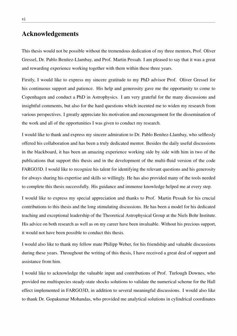
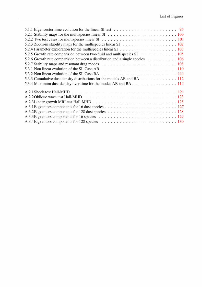
Figure 1.1.1: Gallery adopted from Andrews et al. (2018) corresponding to the Disk Substructures atHigh Angular Resolution Project (DSHARP). It shows the 1.25 mm emission of 20 PPDs.

1.2. Ionization processes in protoplanetary disks 3

1.2 Ionization processes in protoplanetary disks

The presence of magnetic fields in PPDs has been suggested from the observed outflows in the form of

collimated protostellar jets and wide-angle disk winds (e.g., Arce et al., 2007; Bjerkeli et al., 2016).

Taken at face value that disks are magnetized, a clear interest exists on determining the strength of the

magnetic field together with the ionization fraction.

PPDs are subject to different ionization processes that shape the electron and ions density distributions

from the surface layers to the midplane. The estimated temperatures of PPDs suggest that the gas

is generally too cold for thermal ionization to be relevant, except in regions located at r < 1AU

(e.g., Fromang et al., 2002). Far-ultraviolet (FUV) radiation can ionize the surface density layers

of PPDs creating favorable conditions for the magneto-rotational instability (MRI) active layer (e.g.,

Perez-Becker and Chiang, 2011). In addition, ionization beyond the surface layer can be sustained by

the stellar X-ray luminosity, typically assumed to be in the range of LX ∼ 1029 − 1032erg s2 (e.g., Igea

and Glassgold, 1999; Turner et al., 2010; Ercolano and Glassgold, 2013). Cosmic rays (CR) provide

another important contribution to the ionization fraction (e.g., Umebayashi and Nakano, 1981; McCall

et al., 2003) together with radioactive decay (e.g., Turner and Drake, 2009) (primarily the decay of26Al), because they can ionize the medium at the very inner regions of PPDs.

Charged grains can also modify the conductivity of the poorly ionized plasma by adsorbing free

electrons, or through charge exchange due to collisions (e.g., Bai and Goodman, 2009). Recombination

processes are also crucial in PPDs. Positive charges can capture electrons due to different reactions.

The dominant reactions correspond to the dissociative recombination, radiative recombination with

metal ions and reactions that transfer charge from molecular to metal ions (see e.g., Armitage, 2011).

All the estimates indicate that PPDs are poorly ionized and therefore, the coupling between the bulk

of the fluid and the magnetic field might be reduced compared to the fully ionized regime. However,

charged species transfer momentum and energy from the magnetic field onto the neutrals due to

collisions. A rather simple framework to account for the system’s coupled dynamics is the non-ideal

magnetohydrodynamics (MHD) approximation, including the Ohmic and ambipolar diffusions and the

Hall effect (Cowling, 1956; Nakano and Umebayashi, 1986a). These effects strongly depend on the

ionization fraction as well as on the strength of the magnetic field (see e.g., Wardle, 1999; Bai, 2011b).

The importance of self-consistent non-ideal MHD models including chemical reaction networks (for

instance based on Ilgner and Nelson (2006)), has been enhanced by many authors in the last decade

4 1.3. Accretion processes in protoplanetary disks

(e.g. Bai and Stone, 2013; Simon et al., 2015; Gressel et al., 2015; Bai, 2017; Béthune et al., 2017).

Contrary to the classical turbulent flow driven by the magneto-rotational instability (MRI) (Balbus

and Hawley, 1991), all the mentioned works point towards a laminar accretion scenario dominated

by magneto-centrifugal (Blandford and Payne, 1982; Gressel et al., 2015) or magneto-thermal winds

(Lynden-Bell, 1996; Bai et al., 2016).

Stellar X-rays (1 AU, 5 keV)

Cosmic rays (unshielded)

Radioactive decay of 26Al

Likely surfacedensity at 1 AU

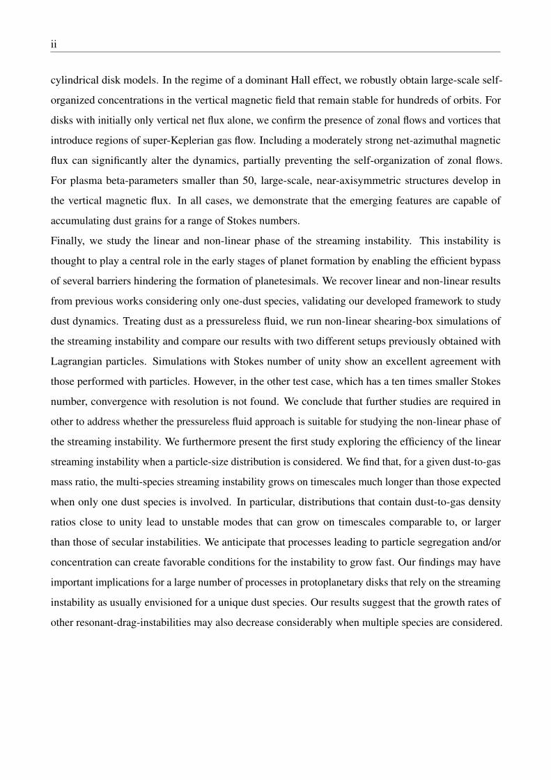
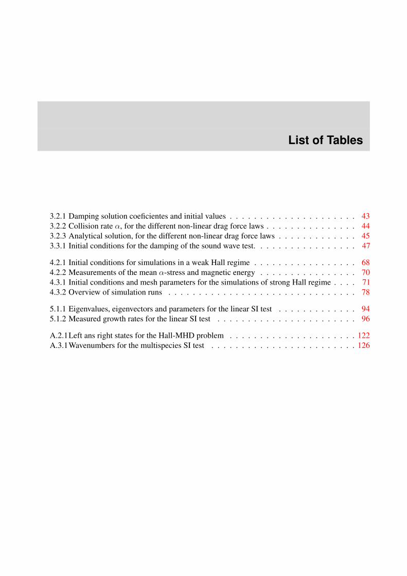
Figure 1.2.1: Figure adopted from Armitage (2011). Ionization rate of different sources (X-rays,cosmic rays and radioactive decay of 26Al) as a function of the column density ∆Σ, measured from thedisk surface.

1.3 Accretion processes in protoplanetary disks

The average lifetime of PPDs is approximately 1− 10 Myr, with typical gas accretion rates of M ∼10−8±1M/yr (Hartmann et al., 1998; Sicilia-Aguilar et al., 2006). The complex astrophysical scenario

of PPDs permits different mechanisms for the radial and vertical transport of angular momentum.

The classical accretion disk model from Lynden-Bell and Pringle (1974) requires a certain amount

of viscosity to remove the angular momentum. Turbulence is usually an efficient source of viscosity

in PPDS. For instance, Maxwell stress can be generated from the MRI (Balbus and Hawley, 1991)

in highly ionized magnetized regions. However, the non-ideal effects as the Ohmic and ambipolar

diffusion can reduce the level of Maxwell stress significantly, and suppress the MRI (Wardle, 1999;

Balbus and Terquem, 2001) due to the low ionization level beyond & 1 AU. Thus, the gas dynamics

becomes laminar in the absence of any source of Reynolds stress when non-ideal MHD effects dominate

the magnetic field evolution (Bai and Stone, 2013).

1.3. Accretion processes in protoplanetary disks 5

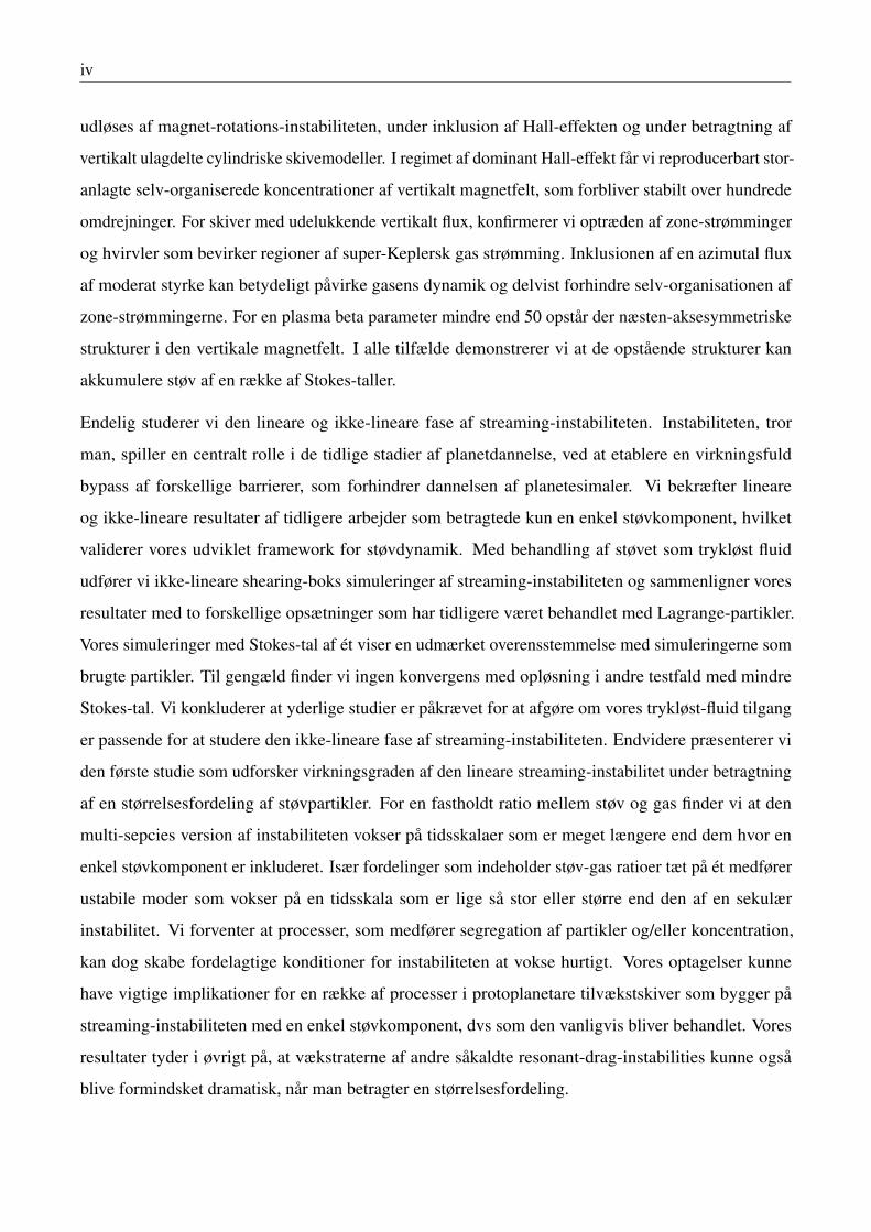
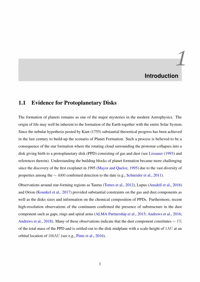
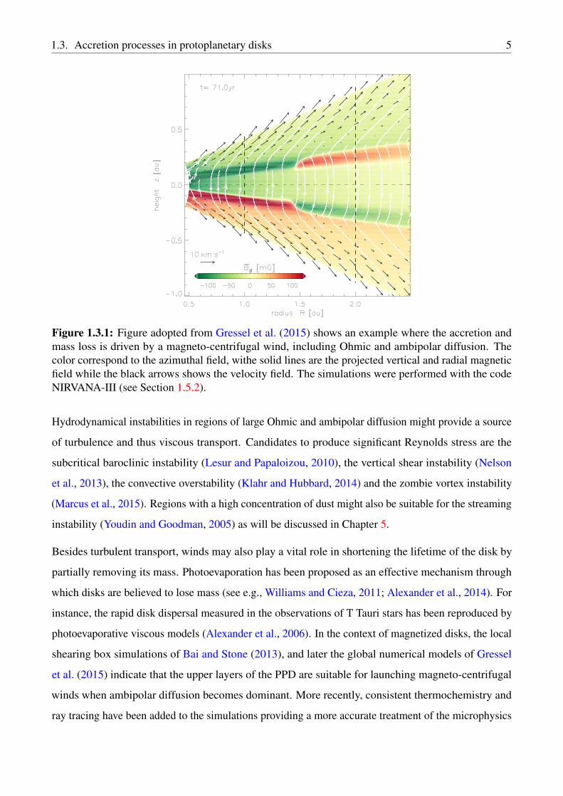
Figure 1.3.1: Figure adopted from Gressel et al. (2015) shows an example where the accretion andmass loss is driven by a magneto-centrifugal wind, including Ohmic and ambipolar diffusion. Thecolor correspond to the azimuthal field, withe solid lines are the projected vertical and radial magneticfield while the black arrows shows the velocity field. The simulations were performed with the codeNIRVANA-III (see Section 1.5.2).

Hydrodynamical instabilities in regions of large Ohmic and ambipolar diffusion might provide a source

of turbulence and thus viscous transport. Candidates to produce significant Reynolds stress are the

subcritical baroclinic instability (Lesur and Papaloizou, 2010), the vertical shear instability (Nelson

et al., 2013), the convective overstability (Klahr and Hubbard, 2014) and the zombie vortex instability

(Marcus et al., 2015). Regions with a high concentration of dust might also be suitable for the streaming

instability (Youdin and Goodman, 2005) as will be discussed in Chapter 5.

Besides turbulent transport, winds may also play a vital role in shortening the lifetime of the disk by

partially removing its mass. Photoevaporation has been proposed as an effective mechanism through

which disks are believed to lose mass (see e.g., Williams and Cieza, 2011; Alexander et al., 2014). For

instance, the rapid disk dispersal measured in the observations of T Tauri stars has been reproduced by

photoevaporative viscous models (Alexander et al., 2006). In the context of magnetized disks, the local

shearing box simulations of Bai and Stone (2013), and later the global numerical models of Gressel

et al. (2015) indicate that the upper layers of the PPD are suitable for launching magneto-centrifugal

winds when ambipolar diffusion becomes dominant. More recently, consistent thermochemistry and

ray tracing have been added to the simulations providing a more accurate treatment of the microphysics

6 1.4. The dust component

and the external heating. These models point towards the presence of magneto-thermal winds where

the flow is driven by pressure gradients instead of tension forces (e.g., Bai et al., 2016; Béthune et al.,

2017; Wang et al., 2019).

1.4 The dust component

Observations of protoplanetary disks indicate a wide range of values for the dust-to-gas ratio from

1% up to 100% (e.g., Ansdell et al., 2016). The evolution of dust particles depends on transport and

collisional processes (e.g., Testi et al., 2014) continuously affecting the grain sizes. Such processes

include coagulation and sticking which may be effective mechanisms to grow µm sized particles into

∼ cm sized grains (e.g., Blum, 2018). However, large particles eventually reach high impact velocities,

and, depending on their intrinsic properties, are prone to fragment. Thus, fragmentation sets a barrier

that prevents particles from growing beyond a certain size (Windmark et al., 2012; Birnstiel et al.,

2016). Besides, the aerodynamical coupling to the gas molecules can induce fast inward (or outward

e.g., Benítez-Llambay et al., 2019) drift of the solids, and thus efficiently remove large particles in

timescales much shorter than the disk lifetime (Whipple, 1972a; Weidenschilling, 1977). How grains

overcome such fragmentation and radial-drift barriers to form km-size bodies has become an enormous

challenge for the current theoretical understanding of PPDs. It is worth mentioning that we will address

a potential mechanism in Chapter to stall the dust radial-drift in 4.

1.5 Review on the codes FARGO3D and NIRVANA-III

1.5.1 FARGO3D

FARGO3D1 is an 3D Eulerian MHD code, with particular emphasis on solving PPDs dynamics and

planet-disk interaction. A comprehensive review of the code is presented in (Benítez-Llambay and

Masset, 2016) and, as a consequence of this work, a new public version is available which includes the

multispecies momentum transfer (Benítez-Llambay et al., 2019). We dedicate a discussion to the major

improvements and new capabilities in Chapter 3 and in this section we summarize the main features.

1 https://fargo3d.bitbucket.io — http://fargo.in2p3.fr

1.5. Review on the codes FARGO3D and NIRVANA-III 7

The code belongs to the family of the so-called ZEUS-type codes, which are based on finite-difference

upwind, dimensionally split methods (Stone and Norman, 1992). Mass and momentum are strictly

conserved, and shock-jump conditions are satisfied in barotropic systems (e.g., isothermal systems).

The code has been developed to exploit High-Performance-Computing (HPC) facilities, and it is capable

of running in CPU- and/or GPU-clusters, with shared or distributed memory. It is written in C with

additional Python scripts and uses a parser to convert C into CUDA language, removing the need of

having CUDA programming skills to modify the code.

∇ Φ

∇ P

INPUTOUTPUTSources

Transport

Figure 1.5.1: Operator splitting scheme in FARGO3D.

It solves the MHD equations in Cartesian, cylindrical and spherical coordinates on a static and staggered2

mesh. Non-uniform meshes can be defined, except in the x-direction (ϕ in cylindrical or spherical

coordinates) which under the current development is always uniform with periodic boundary conditions.

Time integration is first-order while second-order is achieved in the spatial integration. The code

solves the internal energy equation with two possible equations of state implemented, namely locally

isothermal and adiabatic.

A full timestep in the code is divided into two substeps (at least), labeled as the Source and Transport

steps. (i) The Source step solves the momentum and internal energy equations in a non-conservative

form without the advection term. For the momentum, the contribution of the pressure (gas and magnetic),

gravity, and viscosity are included. The work done by the pressure forces is added to the internal

energy (in a non-isothermal case when energy is updated). (ii) The Transport step updates the density,

energy and momentum by solving the advective term, all three using a conservative form of the Euler

equations. The fluxes, defined at the cell-center, are interpolated into the cell-faces using a zone-wise

linear reconstruction with a van Leer’s slope (van Leer, 1977). The transport is done using dimensional2Pressure, density and internal energy are cell-centered while the velocities (and magnetic field) components are

face-centered.

8 1.5. Review on the codes FARGO3D and NIRVANA-III

splitting, first in the z-direction, then in the y-direction and finally in the x-direction.

Defining Q as a generic quantity that follows a transport equation of the form

∂tQ+∇ · (vQ) = S(Q), (1.5.1)

the splitting technique can be written as

∂tQ1 = S(Q0) source step (1.5.2)

∂t

∫

V

Q2dV = −∫

∂V

Q1v · dS transport step (1.5.3)

where V defines a volume and ∂V its boundary. The quantity Q advances a full timestep from an initial

stateQ0 → Q1 and again a full timestep fromQ1 → Q2. A comprehensive explanation of the numerical

procedure that solves the discretized form of these two equations can be found in Benítez-Llambay and

Masset (2016).

The induction equation is solved with the constrained transport (CT) scheme, which guarantees

∂t (∇·B) = 0 to machine precision (Evans and Hawley, 1988). To integrate the induction equation, and

compute the magnetic tension in the momentum equations, FARGO3D uses the method of characteristics

(MOC) (Stone and Norman, 1992).

1.5.2 NIRVANA-III

NIRVANA-III solves the compressible MHD equations describing a time-dependent multi-physics

non-relativistic system (Ziegler, 2004, 2011, 2016). The code is written in C and works in Cartesian,

cylindrical and spherical geometries. NIRVANA-III is MPI parallelized with HPC capabilities for clusters

of CPUs. It includes a block-structured adaptive mesh refinement (AMR) that consist of a set of nested

blocks of size 43 cells. The code solves the conservative fluids equations with isothermal, adiabatic and

polytropic equations of state and a flux conservative total energy formulation. A dual-energy formalism

for high-Mach-number/low-plasma-beta flows is also available.

The spatial integration is done utilizing a semi-discrete (i.e., no time discretization) second-order finite-

volume Godunov scheme. High precision (up to third order in time) is obtained by enabling the 2nd or

3rd Runge-Kutta time integration. NIRVANA-III includes three different Riemann solvers to integrate

1.6. The objectives of this Thesis 9

the MHD equations. A two-dimensional HLL MHD-Riemann solver (Ziegler, 2004; Londrillo and

del Zanna, 2004), and one-dimensional HLL/HLLD MHD-Riemann solver with upwind-interpolated

electric fields (Gardiner and Stone, 2008).

The induction equation is solved using the CT scheme, where for the Hall effect a flux-type HLL

prescription (Lesur et al., 2014) or an operator-split method (O’Sullivan and Downes, 2006) can be

used. Parabolic terms, for instance the Ohmic and ambipolar diffusions, are updated via Strang-split

second-order Runge-Kutta-Legendre super-time-stepping method (Meyer et al., 2012).

Simulations of disks may include the orbital advection scheme that follows from Stone et al. (2008) and

Mignone et al. (2012).

1.6 The objectives of this Thesis

In this Thesis, we address some of the most crucial problems of the current theoretical understanding of

PPDs. Furthermore, we believe that the obtained results may serve as a guideline for future work given

their impact on disk dynamics and planetesimal formation.

In the following we shortly outline the structure of this work and introduce our major goals. A detailed

description and subsequent discussion will then be presented in chapters 3, 4 and 5.

Objective I: Create a multifluid framework accounting for the momentum transfer between charged

species, dust-grains and a gaseous fluid with particular focus on the development of new numerical

schemes to correctly solve the equations describing the dynamics of protoplanetary disks.

Such a framework has been proposed before by several authors. However, the groundbreaking result of

our work — related to this goal — is the presentation of a numerical method that always converges to

the correct solution, that is, the solution obtained by an analytical method as the time goes to infinity.

This result is complemented with general analytical solutions for a diversity of problems, including an

arbitrary number of species. We additionally address the validity of the fluid approach for dust species

recovering linear and non-linear solutions that have been already studied using Lagrangian particles.

The simplicity and efficiency of our numerical method opens new possibilities to study dust dynamics in

PPDs, and potentially other fields. Moreover, we discuss and implement different numerical techniques

10 1.6. The objectives of this Thesis

to solve the Hall effect and Ohmic diffusion. This implies that we do not explicitly solve collisions

between charged and neutral species and instead adopt the non-ideal MHD approximation. We offer a

comparison between different numerical schemes which provides solid grounds to determine whether

the solutions of the non-linear fluid equations are affected by the different numerical approximations.

Objective II: Study the impact of magnetic fields on the dynamics of protoplanetary disks, adopting

the non-ideal magnetohydrodynamics approximation with particular emphasis in the Hall effect and its

role in the evolution of magneto-rotational instability and the self-organization of turbulent flows.

Non-ideal MHD effects introduce a variety of theoretical and numerical challenges because of their

dependency on the ionization fraction and the strength and direction of the magnetic field, which is still

poorly constrained by observations. Thus, parameter explorations with a self-consistent treatment of

the thermodynamics are required, imposing a high computational cost. Besides, a numerical method

to properly solve the Hall effect, that is accurate and stable, is yet to be found. Partially overcoming

these challenges, recent results suggest that self-organized structures, induced by the Hall effect in

turbulent flows, can serve as a bypass for the drift-barrier problem in dust evolution. The pressure

gradient affected by the zonal flows locally modifies the rotational equilibrium from sub-Keplerian to

super-Keplerian azimuthal velocities, stopping the radial-drift of particles as they reach a Keplerian

rotation. Moreover, the local accumulation of dust may favor the formation of planetesimal, which casts

special interest on this issue. Starting from the results of previous authors, we confirm the presence of

self-organized structures induced by the Hall effect as a result of the non-linear dynamics using different

numerical methods. We extend these results by including dust and simulating radially varying disk

models. We find that self-organization is an efficient mechanism for the segregation and accumulation

of dust particles, even in regimes dominated by a strong azimuthal magnetic flux.

Objective III: Determine the linear growth of the streaming instability in local regions of

protoplanetary disks considering multiple dust species that can be described by a particle-size

distribution.

The streaming instability is thought to play a central role in the early stages of planet formation by

enabling the efficient bypass of several barriers hindering the formation of planetesimals. However, a

study of the linear phase of this instability has never been done including more that one particle size.

Taking that as a motivation, we present the first study exploring the efficiency of the linear streaming

1.6. The objectives of this Thesis 11

instability when a particle-size distribution is considered and arrive at some remarkable conclusions: We

find that the multi-species streaming instability grows on timescales much longer than those expected

when only one dust species is involved. In particular, distributions that contain dust-to-gas density ratios

that are close to order unity lead to unstable modes that can grow on timescales comparable, or larger,

than those of secular instabilities. Our findings may have important implications for a large number of

processes in protoplanetary disks that rely on the streaming instability as usually envisioned for a single

dust species. in addition, our results suggest that the growth rates of other resonant-drag-instabilities

may also decrease considerably when multiple species are considered.

The persisting uncertainty of key parameters for the dynamics of interest dissuades us from including

the mentioned physical processes in a single study. Instead, to explore the most important questions,

we adopt a rather conservative approach, setting-up a controlled framework with a set of well-defined

and isolated problems for each of the stated objectives. The diversity of the problems discussed within

this work will address particular aspects of the dynamics of the protoplanetary disk, and vary from

analytical linear stability calculations to fully non-linear numerical simulations.

2Protoplanetary Disk Dynamics

Protoplanetary disks are composed of a mixture of partially ionized gas and dust particles. In this

work, we assume that the mixture can be modeled as a plasma in local thermal equilibrium; hence,

the gas molecules, ions, and electrons follow a Maxwellian distribution. Thus, the dynamics of the

system is fully described by the transport equations obtained after averaging the Boltzmann equation

(e.g. Braginskii, 1965; Draine, 1986; Chernoff and Shapiro, 1987; Benilov, 1997). The charged

species interact with the magnetic and electric fields, which evolve according to the Maxwell equations

neglecting the displacement current. In addition, the species interchange momentum due to elastic

collisions which significantly affects the conductivity of the plasma (e.g., Cowling, 1956; Norman and

Heyvaerts, 1985; Wardle, 1999; Falle, 2003; Pandey and Wardle, 2008). In our framework, mass and

energy transfers are neglected. Dust grains can also affect the conductivity of the plasma in PPDs (e.g.,

Bai, 2011b), but we adopt a more conservative approach considering dust particles to be neutral. In the

strong coupling regime, the dust’s interaction with the gas due to drag forces allows us to describe its

dynamics as a pressureless fluid (e.g. Cuzzi et al., 1993; Garaud et al., 2004).

In this chapter, we present the equations that describe the dynamics of PPDs in the context of non-ideal

MHD and set the framework of our work (see Section 2.1). We neglect radiative transfer, cooling,

and viscous processes as well as self-gravity and chemical reactions. Also, we do not include a self-

consistent ionization model. A brief discussion on the validity of the non-ideal MHD approximation is

presented in Section 2.2.

12

2.1. Equations 13

2.1 Equations

The complete set of equations describing a system of a neutral gas coupled to the magnetic field due to

collisions with ions and electrons, and N − 1 dust-species reads as

∂tρg +∇·(ρgvg) = 0 ,

∂tρd,j +∇·(ρd,jvd,j) = 0 ,

ρg(∂tvg + vg ·∇vg) = −∇P − ρg∇Φ + J×B +Fg ,

ρd,j(∂tvd,j + vd,j ·∇vd,j) = −ρd,j∇Φ +Fd,j , with j = 1, . . . , N − 1. (2.1.1)

The density and velocity are defined as ρg, vg and ρdj , vd,j for the gas and dust j-species, respectively.

Importantly, both species are considered as neutral fluids, but as we will discuss in Section 2.2, a neutral

fluid experiences a Lorentz force as a consequence of the collisions with the charged species.

The time evolution of the magnetic field is determined by the induction equation

∂tB = ∇× (vg×B)−∇×E , (2.1.2)

where the electric field is obtained from the generalized Ohm’s law,

E = ηOJ + ηHJ×eB − ηAJ×eB×eB, (2.1.3)

with eB the unit vector along B, and where the current density is J ≡ µ−10 ∇×B. The three terms of

Eq. (2.1.3) correspond to the Ohmic diffusion (O), the Hall effect (H) and the ambipolar diffusion (A).

We discuss the validity of this equation together with the expressions for the diffusivities in Section 2.2.

We adopt a locally isothermal equation of state where the sound speed, cs, satisfies c2s = P/ρg.

The drag force, F, accounts only for the collisions between the gas and the dust species,

Fg = −ρg

N−1∑

j=1

αgj (vg − vd,j) ,

Fd,j = −ρd,jαjg (vd,j − vg) ,

(2.1.4)

14 2.1. Equations

with αgj the collision rate between the gas and the j-dust-species. This collision rate parameterizes the

momentum transfer per unit time and is, in general, a function of the physical properties of the species

and their mutual relative velocity. Momentum conservation implies

ρlαlj = ρjαjl . (2.1.5)

In the following chapters we will solve this set equations, or a subset, depending on the problem.

In Section 2.2, we extend our discussion to provide some insight on the validity of the single-fluid

induction equation.

2.1.1 Dust as a pressureless fluid

In the case of a system composed of gas and several dust species, dust can be modeled as a pressureless

fluid. It is clear that this approximation fails in describing the dynamics of systems dominated by

crossing trajectories, a regime prone to develop when gas and dust species are coupled very weakly.

In this work, we neglect collisions between dust species, and hence dust species only interact indirectly

via their coupling with the gas. After using the condition (2.1.5), the collision rate, αlj , can be written

as

αlj ≡ αlδjg + εjαjδgl , (2.1.6)

with εj = ρj/ρg and δig the Kronecker delta.

The inverse of the collision rate αl is defined as the stopping time, tsl. In the context of PPDs, the

stopping time is usually represented by the Stokes number, Ts, which is a dimensionless parameter that

characterizes the stopping time in units of the inverse local rotation frequency1, Ω−1, such that

tsl = TslΩ−1 . (2.1.7)

The Stokes number depends on the properties of the gas and the dust-grains. When the size of the dust

particle is smaller than 9λmfp/4, with λmfp being the gas mean-free-path, the grains are in the Epstein

regime, and the Stokes number can be written as (see e.g., Epstein, 1924; Safronov, 1972; Whipple,

1It can be adopted another relevant timescale instead of the one given by the rotation frequency

2.1. Equations 15

1972b; Draine and Salpeter, 1979; Takeuchi and Lin, 2002),

Ts = Ω

√π

8

ρpa

ρgcs

, (2.1.8)

where the dust grain is assumed to be spherical with radius a and a material density ρp. In this work,

we always assume Ts to be constant.

2.1.2 Particle-size distributions

The size distribution of solids in PPDs may extend from µm to several km. Dust evolution processes

shape the distribution, and thus, it becomes a function of space and time. However, as an approximated

initial distribution we consider a power-law of the form n(a) ∝ aq, which correspond to the interstellar

medium particle-size distribution obtained from extinction measurements over the wavelength from

0.1µm < λ < µm (e.g., Dohnanyi, 1969; Mathis et al., 1977).

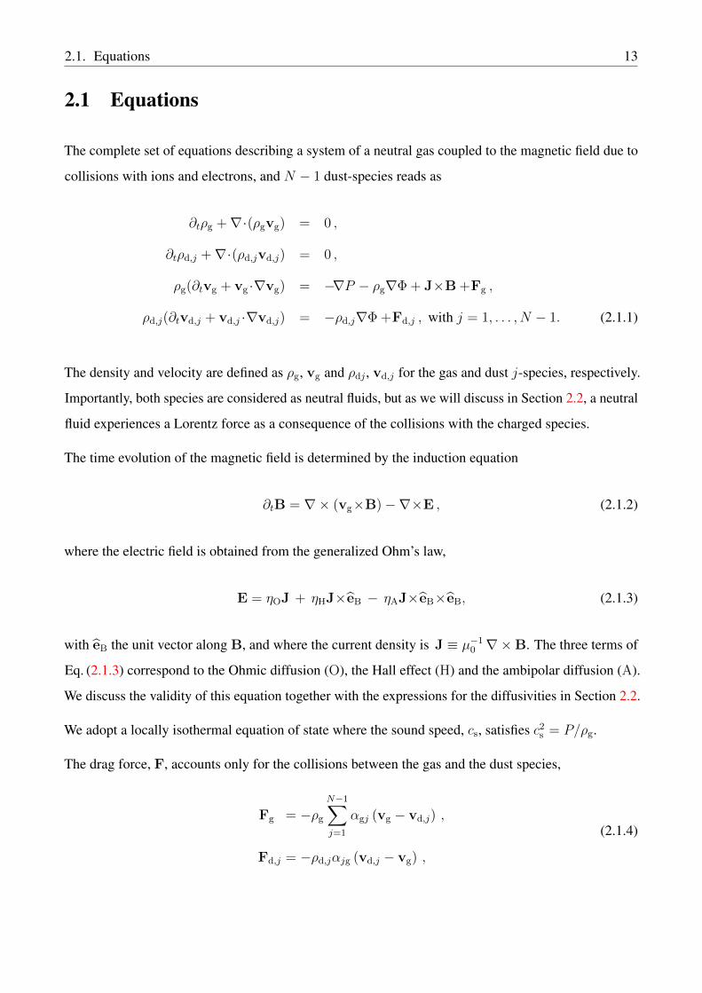
Figure 2.1.1: Schematic representation of a particle-size distribution where the particle size isproportional to the Stokes number.

In this work, we do not evolve the continuous particle-size distribution in time. We adopt a discrete

approximation that is characterized by the total dust-to-gas density ratio, ε, a range of Stokes numbers

properly bound by a minimum and a maximum, ∆Ts = [Ts,min, Ts,max], and the total number of species

N associated with a distinct Stokes number, Ts,j , with j = 1, . . . , N . The total mass of the distribution

remains constant when varying N , i.e.,∑N

j=1 εj = ε, where εj is the dust-to-gas density ratio associated

with a given dust species.

16 2.2. Non-Ideal Magnetohydrodynamics

Assuming that all the grains are spherical with radius a, we see that ρd(a) ∝ a3+q. In addition, in a local

approximation where Ω, ρg and cs are constant, the size a ∝ Ts. Thus, the density ratio εj is obtained

after integrating over a given Stokes number interval [Ts,j+1, Ts,j] as

εjε

=

T 4+qs,j+1 − T 4+q

s,j

T 4+qs,max − T 4+q

s,min

if q 6= 4

ln (Ts,j+1) / ln (Ts,j)

ln (Ts,max) / ln (Ts,min)if q = 4 .

(2.1.9)

2.2 Non-Ideal Magnetohydrodynamics

The non-ideal MHD approximation has been extensively discussed in a general framework since

Cowling (1956) and more recently applied to PPDs due to the low ionization fraction and the expected

presence of magnetic fields (e.g., Wardle, 1999). A full derivation of Eqs. (2.1.1)-(2.1.3) (neglecting the

dust species) can be found in Nakano and Umebayashi (1986a) and Nakano and Umebayashi (1986b).

In the following, we briefly describe the important steps and assumptions.

We start by considering a set of N charged species that interchange momentum via collisions with a

neutral species. We define the density and velocity of the neutral species as ρn and vn, while for each

charged species, we use ρi and vi. Defining d/dt = ∂t + v · ∇, the momentum equations read as

N∑

j=1

ρnνin(vi − vn)−∇Pn − ρndvndt

= 0 ,

Zieni (E + vi ×B)− ρiνin(vi − vn)−∇Pi − ρidvidt

= 0 , for i = 1, . . . , N, (2.2.1)

where ni, Zie and mi are the number density, charge and mass of the i-species, respectively, with e

being the charge of the electron. The pressure for the i-species is defined as Pi, and we are assuming

that the pressure tensor is isotropic for all the species. Collisions between charged species are neglected,

thus the collision frequency, νin, is defined as

νin = ρn〈σvi〉

mi +mn

, (2.2.2)

where 〈σvi〉 is the rate coefficient for the momentum transfer between a neutral and a charged species,

2.2. Non-Ideal Magnetohydrodynamics 17

with mass mn and mi, respectively (e.g., Draine, 1986). The viscous damping timescale is defined as

τin = 1/νin. (2.2.3)

The main assumptions for the non-ideal MHD approximation are (i) charge neutrality, (ii) low ionization

fraction and (iii) viscous damping much shorter than the dynamical timescale, i.e.,

N∑

j=1

eZini = 0, ρi/ρn 1, τin tdyn. (2.2.4)

2.2.1 Single-fluid momentum equation

Defining the density and velocity as ρ and v of total fluid mixture, we have

ρ = ρn +N∑

j=1

ρj = ρn

(1 +

N∑

j=1

ρjρn

)' ρn , (2.2.5)

v =1

ρ

(ρnvn +

N∑

j=1

ρjvj

)' vn , (2.2.6)

where we used condition (ii) of 2.2.4. Now, adding Eqs. (2.2.1) we obtain

ρndvndt

= −∇P + J×B , (2.2.7)

with P = Pn+∑

j Pj and J =∑

j eZjnjvj . This explains why in Eq. (2.1.1) a neutral fluid experiences

a Lorentz force.

2.2.2 Induction equation

The Maxwell equations determine the evolution of the electric and magnetic field. In PPDs, the

velocities satisfy v c, with c the speed of light, and we can safely neglect the displacement current,

then the Faraday and Ampere’s law read as

∂B

∂t= −∇× E, J =

1

µ0

∇×B . (2.2.8)

18 2.2. Non-Ideal Magnetohydrodynamics

The electric field, E, can be obtained from the momentum equations of the charged species, which

leads to a generalized Ohm’s law. In the co-moving frame of the neutrals, the electric field read as

E = E + vn ×B. (2.2.9)

In addition, we recast the pressure and inertial terms of the charged species into a new variable h:

hi = −∇Pi − ρidvidt

. (2.2.10)

Defining relative velocity between the neutral fluid and the i-species as vri = vi − vn, the momentum

equation of the positive charged species, k, and the electron species, in the frame of the neutral fluid,

reads as

Zkenk

(E + vrk ×B

)− ρkτk

vrk + hk = 0 , (2.2.11)

Zeene

(E + vre ×B

)− ρeτe

vre + he = 0 . (2.2.12)

Taking the electric field from the Eq. (2.2.11) into Eq. (2.2.12), subsequently solving the resulting

equation for vrk, and using the condition hn +∑

j ρj/τjvrj = 0 in combination with Eq. (2.2.7), leads

to2

(A1 +

A2

τeωe

)vre −

(A1 +

A2

τeωe

)Rvre = J×B + F(hk,he, A1, A2, τk, τe, ωk, ωe) , (2.2.13)

where the matrix R defines a rotation in a plane orthogonal to B by an angle −π/2. The gyrofrequency,

ωj , is

ωj = Zje|B|mjc

, (2.2.14)

and the coefficients, A1, and, A2, are defined as

A1 =N∑

j=1

ρjω2j

τj(1/τ 2j + ω2

j )A2 =

N∑

j=1

ρjωjτ 2j (1/τ 2

j + ω2j ). (2.2.15)

The conditions 2.2.4 imply that all the terms in the L.H.S of Eq. (2.2.15) which are represented by the

function F are negligible with respect to J×B (Nakano and Umebayashi, 1986a). Thus, the electron

2This is done assuming a Cartesian coordinate system with B parallel to z.

2.2. Non-Ideal Magnetohydrodynamics 19

velocity satisfies (A1 +

A2

τeωe

)vre −

(A1 +

A2

τeωe

)Rvre = J×B. (2.2.16)

Neglecting he in the electron momentum equation (2.2.12), the balance between the Lorentz force and

the collisional force leads to a generalized Ohm’s law, that is,

E = vre ×B− me

eτevre . (2.2.17)

Replacing the solution of Eq. (2.2.16) and transforming back to the original reference frame we obtain

E = −vn ×B +1

σ1

J +1

σ2

J×B− 1

σ3

(J×B)×B , (2.2.18)

with

σ1 =N∑

j=1

(Zje)2τjnj

mj

, σ2 =A2

1 + A22

A2|B|, σ2 =

1

A1/(A21 + A2

2)− 1/(σ1|B|2). (2.2.19)

2.2.3 Diffusion coefficients

The inverse of the conductivities σ1, σ2 and σ3 define the Ohmic (ηO), Hall (ηH) and ambipolar (ηA)

diffusion coefficients used to write the induction equation 2.1.2. These coefficients can be expressed in

terms of the Hall and Pedersen conductivities defined as σO, σH and σP (Wardle, 1999, 2007, see e.g.,)

which depend on the Hall parameter, defined as

βj =|Zj|emj

|B|τjcρn

. (2.2.20)

Thus, we will adopt the following expressions for the diffusion coefficients

ηO =c2

4πσO

, ηH =c2

4πσ⊥

σH

σ⊥, ηA =

c2

4πσ⊥

σP

σ⊥− ηO , (2.2.21)

where σ⊥ =√σ2

H + σ2P.

20 2.2. Non-Ideal Magnetohydrodynamics

If charged particles other than ions and electrons are negligible, the diffusion coefficients simplify to

(Wardle, 1999; Pandey and Wardle, 2008; Bai, 2011a)

ηO =c2γemeρn4πe2ne

∼ 1

xe,

ηH =c|B|

4πene∼ 1

xe

|B|ρn

,

ηA =|B|2

4πνinρnρi∼ 1

xe

( |B|ρn

)2

, (2.2.22)

where xe = ne/n is the ionization fraction, ρi is the ion density, ne is the electron number density and

me is the electron mass. Under this approximation and in a weakly ionized medium, i.e., ρe/ρn <

ρi/ρn 1, Pandey and Wardle (2008) found that the non-ideal MHD equations are valid if the

characteristic frequency of the system of interest, ω, satisfies

ω .√ρg

ρi

βe1 + βe

νin , (2.2.23)

with βe and βi being the Hall parameter of the electrons and ions, respectively. This approximation

provides a simple way to characterize the importance of the three non-ideal MHD terms as a function

of the Hall parameter. Thus, the ratio of the Hall term and Ohmic diffusion depends on the electron

Hall parameter while the ratio between the Hall term and the ambipolar diffusion depends on the ion

Hall parameter, that is

H

O∼ βe ,

A

H∼ βi. (2.2.24)

The regime dominated by Ohmic diffusion corresponds to the case βi βe 1 while the ambipolar

diffusion will dominate the evolution of the magnetic field in the case where 1 βi βe. The Hall

effect dominates the regime in between, that is βi 1 βe, this corresponds to a regime where ions

are well coupled to the neutral fluid, but electrons can drift.

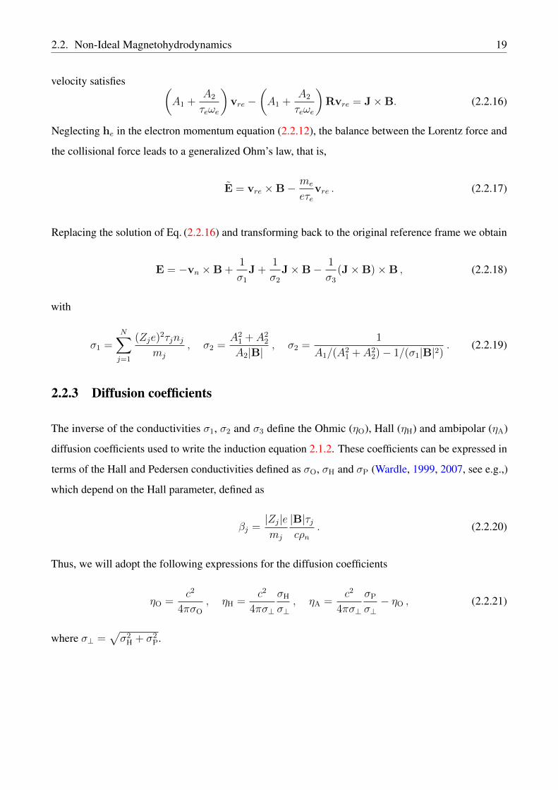
Figure 2.2.1 (from Armitage (2015)) shows the specific regions of a PPD in which of each of the

non-ideal MHD effects dominates. This shows that the Hall effect is important in the inner regions of

the protoplanetary disk . 30AU and close to the midplane. In these regions the Hall frequency ωH is

smaller than the dynamical frequency and the Hall length, LH, is larger than the dynamical length scale.

2.3. The Magneto-Rotational Instability (MRI) 21

Both quantities scale with the ion density as

ωH ∼ρiρωci , LH ∼

ρ

ρi

vA

νinβ−1i , (2.2.25)

where ωci is the ion cyclotron frequency. The smaller the ionization fraction, the larger the Hall length,

and thus the Hall effect becomes important at that scale. Typical values for the Hall frequency and the

Hall length in PPDs can be found in Table 3 of Pandey and Wardle (2008), where, assuming a minimum

mass solar nebula disk model (Hayashi, 1981) with a magnetic field of B ∼ 10−2G, the Hall length is

the order of LH ∼ 105km at r = 5 AU.

Figure 2.2.1: Figure adopted from Armitage (2015) that shows the importance of the non-ideal MHDeffects in a PPD, depending on the magnetic field strength and the number density of neutral, n.

2.3 The Magneto-Rotational Instability (MRI)

In the last decade, the understanding of the accretion scenario of PPDs has moved from a turbulent

viscosity induced by the MRI (Balbus and Hawley, 1998), to a laminar and almost inviscid flow relying

on magneto-centrifugal (Bai and Stone, 2013; Gressel et al., 2015) and magneto-thermal (Bai et al.,

2016) winds for angular momentum transport. Generally, one can argue that turbulent and laminar

processes may coexist in the complex environment of PPDs. Thus, regardless the importance of the

MRI for accretion, it can always affect the dynamics locally. For instance, it provides an efficient

mechanism to stall the radial-drift of the dust, as we will show in this work (see Chapter 4). In the

22 2.3. The Magneto-Rotational Instability (MRI)

following, we briefly describe the nature of the MRI and its evolution when considering a weakly

ionized plasma.

Lets consider a differentially rotating disk with angular frequency Ω(r) = Ω0rq, that is threaded by

a vertical magnetic field, B = Bz, and the fluid is frozen to the field lines, i.e., ideal MHD regime.

Furthermore, lets assume that the flow is incompressible and waves propagate with the Alfvén speed,

vA = B/√µ0ρ. A locally perturbed fluid parcel that is removed from its orbital equilibrium to an

inward position will rotate slightly faster than in its equilibrium state and furthermore will induce a

displacement of the magnetic field lines. The magnetic tension will try to restore the field lines to the

initial vertical equilibrium pulling the parcel to a new orbital position. If the magnetic tension is weak

enough, a buckling of the field lines can occur, increasing the magnetic tensions and leading to runaway

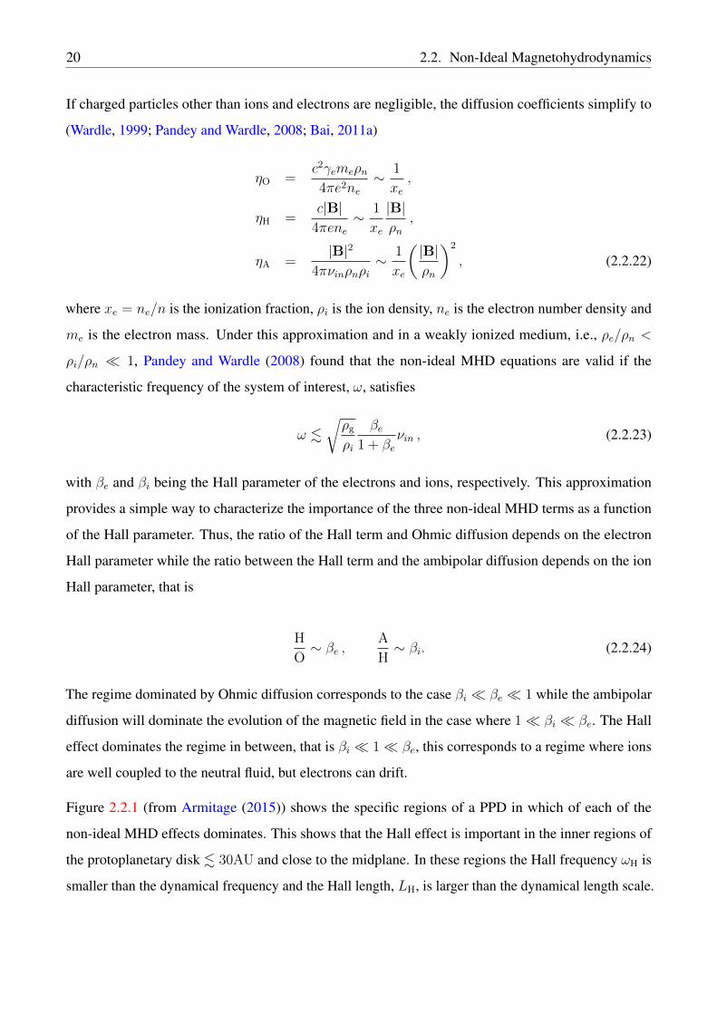
growth.

J x B

J x B

B0+ δB

1

2v

v

rφz

x

B0

1

2

Figure 2.3.1: Left panel: Figure from Wardle and Salmeron (2012) that sketch the configurationadopted to illustrate the nature of MRI. The fluid perturbations represented by blue circles carry withthem the vertical field line (black solid line), which will exert a tension force trying to restore theequilibrium state. Right panel: Figure from Flock et al. (2011) shows the non-linear evolution of therms velocity in a global simulation of a PPD.

When the linear perturbation propagates along a periodic vertical direction, that is δB =

Re(∑

n δBneiknz−iωnt

), the instability criteria (that gives a pure imaginary frequency ωn) reads as

k2nv

2A +

dΩ2

d ln r< 0 , (2.3.1)

where kn is a vertical wavenumber (Balbus and Hawley, 1991). For arbitrary small and real

wavenumbers, this criterion imposes a necessary condition, q < 0, which is satisfied in PPDs that have

a Keplerian rotation frequency, i.e., q = −3/2. After the linear phase, the instability saturates, giving a

2.3. The Magneto-Rotational Instability (MRI) 23

turbulent self-regulated flow that dominates the dynamics (e.g., Balbus and Hawley, 1998).

In the case of a Keplerian disk, the maximum growth rate is given by ω = 3/4Ω and the associated

vertical wavenumber is kmax =√

15Ω/4vA. The three non-ideal effects significantly affect the

properties of the MRI (Wardle, 1999; Sano and Stone, 2002; Bai and Stone, 2013), for instance in a Hall

dominated regime the wavenumber associated with the maximum growth is given by k2max = 2Ω/ηH

(e.g., Mohandas and Pessah, 2017).

The coupling between the magnetic field and the neutral fluid at a length scale proportional to the

characteristic wavelength of the MRI unstable modes is given by the Elsasser numbers (e.g. Wardle and

Salmeron, 2012),

ΛO ≡v2A

ηOΩ, ΛA ≡

v2A

ηAΩ, ΛH ≡

v2A

ηHΩ, (2.3.2)

which are dimensionless parameter commonly used to describe the importance of the non-ideal effects

at different locations of the PPDs. Moreover, the relative importance of the Hall term can, in general,

be defined via the Hall length that was introduced in Section 2.2 and is redefined here as,

LH ≡ ηH v−1A , (2.3.3)

(Pandey and Wardle, 2008; Kunz and Lesur, 2013). This definition will be adopted within this work

when addressing the strength of the Hall diffusion in our disk models. This is motivated by the work

of Kunz and Lesur (2013), where, employing a an incompressible non-stratified shearing box disk

model, they found that if LH/H ∼> 0.2 the MRI saturates to a new regime where the self-organization

mechanism starts to be operative. The typical length, H , can be adopted as the hydrostatic scale height

of a vertical stratified disk. Thus, LH/H provides a dimensionless control parameter for this new

saturation regime of the MRI.

3Numerical Scheme for Multispecies Momentum Transfer

In this chapter we will focus on the momentum transfer between multiple species. First, we present an

asymptotically and unconditionally stable numerical scheme to solve the collisions between an arbitrary

number of species.

Aimed at studying dust dynamics, we implement this numerical method in the publicly available code

FARGO3D. To validate our implementation, we develop a test suite for an arbitrary number of species,

based on analytical or exact solutions of problems related to perfect damping, damped sound waves

and global gas-dust radial drift in a disk. In particular, we obtain first-order, steady-state solutions for

the radial drift of multiple dust species in protoplanetary disks, in which the pressure gradient is not

necessarily small.

We show that the implementation in the MHD code FARGO3D will always converge to the correct

analytical asymptotic equilibrium solution. We then conclude that our scheme is suitable, and very

robust, to study the self-consistent dynamics of several fluids. In particular, it can be used for solving the

collisions between gas and dust in protoplanetary disks, with any degree of coupling. To our knowledge,

such a complete assessment of the numerical scheme has never been done, so it constitutes one of the

major achievements of the present work.

24

3.1. Implicit update 25

3.1 Implicit update

In this section we will focus on the numerical solution of the velocity for a set of colliding species.

The method assumes a linear drag force in the velocity1 and all the collision frequencies satisfy the

symmetry relation defined in Eq. (2.1.5). After introducing the implicit update, we show that it conserves

momentum to machine precision. In addition, we demonstrate several properties of the numerical

scheme in order to show that it is asymptotically stable, that is, the numerical error is always bound and

converges to zero as the timestep, or the number of integration steps, increases.

Considering only the collision term in the momentum equation (see Eq. (2.1.1)) the acceleration of the

i-species reads asdvidt

= − 1

ρi

N∑

j=1

αij (vi − vj) . (3.1.1)

Note that Eq. (3.1.1) is a first-order differential equation, and can be solved by:

(i) Analytical methods: Such a linear system defines a regular eigenvalue problem. This method is

probably the best choice if the problem is isolated because there is no need of any discretization,

i.e., no truncation error. The system is non-symmetric, and a transformation is needed in other to

use an efficient eigenvalue solver. As a result, two matrix transformations are required, plus the

eigenvalue solver, to obtain a full update of the velocity, which makes this approach numerically

expensive as the number of species increases. Furthermore, if the equation is combined with

numerical integrators (for example in an MHD code), the numerical errors of the solution will be

dominated by the step with lowest precision. Thus, it might be redundant to use an such an exact

method for solving the collisions. Finally, if the collision rate depends on the velocity, the system

becomes non-linear and, as we will show, this is not a limitation for our implicit method.

(ii) Time-explicit method: Explicit methods may provide a rather fast convergence to the equilibrium

solution in comparison to the implicit integration. However, large collision rates in an explicit

update impose a very restrictive stability condition when solving for a mixture of multiple fluids

(see e.g. Vorobyov et al., 2018; Stoyanovskaya et al., 2018). This makes the computation slower,

significantly affecting the performance of a code.

(iii) Time-implicit method: This is the adopted method in this work and it will be discussed in this

1In Section 3.2.4.5 we show that the method recover solutions in non linear drag force regimes.

26 3.1. Implicit update

section.

The most straightforward formula for an implicit update is obtained by expressing Eq.3.1.1 in finite

differences and evaluating the velocities on the R.H.S. in the advanced time (backward Euler method),

i.e.,vn+1i − vni

∆t= −

∑

j 6=iαnij(vn+1i − vn+1

j

). (3.1.2)

Eq. (3.1.2) corresponds to a set of 3N linear algebraic equations for the unknown vn+1 velocities, which

can be written in a more convenient way as

vn+1i

[1 + ∆t

∑

j 6=iαnij

]−∆t

∑

j 6=iαnijv

n+1j = vni . (3.1.3)

A more compact form of Eq. (3.1.3) is obtained by defining the column vectors

Vk = [ v1 · ek , . . . , vN · ek ]T , (3.1.4)

that is, Vk is formed by the projection of the velocity of each species along the direction of the unit

vector ek, with k = 1, 2, 3. The superscript T stands for transpose. With this, Eq. (3.1.3) can be written

as a matrix equation

TVn+1k = Vn

k , (3.1.5)

where

T = I + ∆tM , (3.1.6)

is an N ×N matrix, I is the identity matrix, and the (i, j)-element of the matrix M is

Mij ≡N∑

k 6=iαnikδij − αnij (1− δij) . (3.1.7)

The first and second terms in Eq. (3.1.7) set the diagonal and non-diagonal elements of M, respectively.

Because T is nonsingular (see Section 3.2.2.1), the solution of Eq. (3.1.5) exists.

Stone (1997) showed a simple solution of Eq. (3.1.5) for two fluids. However, the complexity of these

solutions rapidly increases with N , making them impractical. Thus, we prefer to solve Eq. (3.1.5)

numerically by means of Gaussian elimination with partial pivoting (see e.g. Press et al., 2007, Chapter

2).

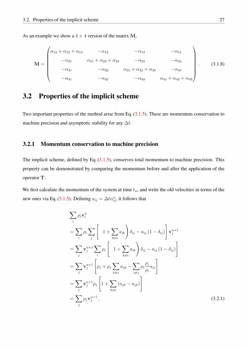
3.2. Properties of the implicit scheme 27

As an example we show a 4× 4 version of the matrix M,

M =

α12 + α13 + α14 −α12 −α13 −α14

−α21 α21 + α23 + α24 −α23 −α24

−α31 −α32 α31 + α32 + α34 −α34

−α41 −α42 −α43 α41 + α42 + α43

. (3.1.8)

3.2 Properties of the implicit scheme

Two important properties of the method arise from Eq. (3.1.5). These are momentum conservation to

machine precision and asymptotic stability for any ∆t.

3.2.1 Momentum conservation to machine precision

The implicit scheme, defined by Eq. (3.1.5), conserves total momentum to machine precision. This

property can be demonstrated by comparing the momentum before and after the application of the

operator T.

We first calculate the momentum of the system at time tn, and write the old velocities in terms of the

new ones via Eq. (3.1.5). Defining aij = ∆tαnij , it follows that

∑

i

ρivni

=∑

i

ρi∑

j

[(1 +

∑

k 6=iaik

)δij − aij (1− δij)

]vn+1j

=∑

j

vn+1j

∑

i

ρi

[(1 +

∑

k 6=iaik

)δij − aij (1− δij)

]

=∑

j

vn+1j

[ρj + ρj

∑

k 6=iajk −

∑

i6=jρiρjρiaji

]

=∑

j

vn+1j ρj

[1 +

∑

k 6=i(ajk − ajk)

]

=∑

j

ρjvn+1j , (3.2.1)

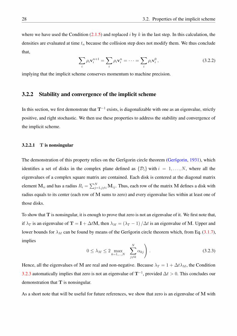
28 3.2. Properties of the implicit scheme

where we have used the Condition (2.1.5) and replaced i by k in the last step. In this calculation, the

densities are evaluated at time tn because the collision step does not modify them. We thus conclude

that,∑

i

ρivn+1i =

∑

i

ρivni = · · · =

∑

i

ρiv0i , (3.2.2)

implying that the implicit scheme conserves momentum to machine precision.

3.2.2 Stability and convergence of the implicit scheme

In this section, we first demonstrate that T−1 exists, is diagonalizable with one as an eigenvalue, strictly

positive, and right stochastic. We then use these properties to address the stability and convergence of

the implicit scheme.

3.2.2.1 T is nonsingular

The demonstration of this property relies on the Geršgorin circle theorem (Geršgorin, 1931), which

identifies a set of disks in the complex plane defined as Di with i = 1, . . . , N , where all the

eigenvalues of a complex square matrix are contained. Each disk is centered at the diagonal matrix

element Mii and has a radius Ri =∑N

j=1,j 6=i Mij . Thus, each row of the matrix M defines a disk with

radius equals to its center (each row of M sums to zero) and every eigenvalue lies within at least one of

those disks.

To show that T is nonsingular, it is enough to prove that zero is not an eigenvalue of it. We first note that,

if λT is an eigenvalue of T = I + ∆tM, then λM = (λT − 1) /∆t is an eigenvalue of M. Upper and

lower bounds for λM can be found by means of the Geršgorin circle theorem which, from Eq. (3.1.7),

implies

0 ≤ λM ≤ 2 maxk=1,...,N

(N∑

j 6=kαkj

). (3.2.3)

Hence, all the eigenvalues of M are real and non-negative. Because λT = 1 + ∆tλM , the Condition

3.2.3 automatically implies that zero is not an eigenvalue of T−1, provided ∆t > 0. This concludes our

demonstration that T is nonsingular.

As a short note that will be useful for future references, we show that zero is an eigenvalue of M with

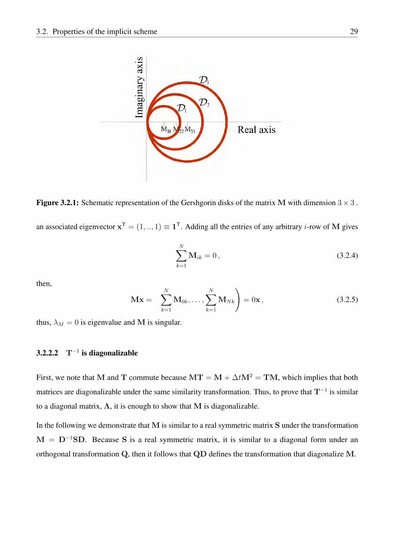
3.2. Properties of the implicit scheme 29

Figure 3.2.1: Schematic representation of the Gershgorin disks of the matrix M with dimension 3× 3 .

an associated eigenvector xT = (1, .., 1) ≡ 1T. Adding all the entries of any arbitrary i-row of M gives

N∑

k=1

Mik = 0 , (3.2.4)

then,

Mx =

(N∑

k=1

M0k, . . . ,N∑

k=1

MNk

)= 0x , (3.2.5)

thus, λM = 0 is eigenvalue and M is singular.

3.2.2.2 T−1 is diagonalizable

First, we note that M and T commute because MT = M + ∆tM2 = TM, which implies that both

matrices are diagonalizable under the same similarity transformation. Thus, to prove that T−1 is similar

to a diagonal matrix, Λ, it is enough to show that M is diagonalizable.

In the following we demonstrate that M is similar to a real symmetric matrix S under the transformation

M = D−1SD. Because S is a real symmetric matrix, it is similar to a diagonal form under an

orthogonal transformation Q, then it follows that QD defines the transformation that diagonalize M.

30 3.2. Properties of the implicit scheme

To prove that M is similar to S, we define the similar diagonal transformation

Dij ≡√ρ0

ρjδij = ηjδij , (3.2.6)

for any arbitrary ρ0, and show that S = D−1MD is symmetric. We first calculate

(D−1M

)ij

=∑

k

D−1ik Mkj

=∑

k

ηkδik

(∑

l 6=kαklδkj − αkj (1− δkj)

)

=∑

k

ηkδik∑

l 6=kαklδkj −

∑

k

ηkδikαkj (1− δkj)

=∑

l 6=jηjαjlδij − ηiαij (1− δij) . (3.2.7)

from which we can obtain Sij

Sij =(D−1MD

)ij

=∑

k

(D−1M

)ik

Dkj

=∑

k

[∑

l 6=kηkαklδik − ηiαik (1− δik)

]η−1j δkj

=∑

k

ηkη−1j δik

∑

l 6=kαkl −

∑

k

ηiη−1j αi,k (1− δik) δkj

=∑

l 6=kαjlδij − αijηiη−1

j (1− δij) . (3.2.8)

Finally, the symmetry of S is proven by using Eq. (2.1.5), i.e., αij = αjiη2j η−2i .

Sij = −αijηiη−1j (1− δij) = −αjiηjη−1

i (1− δij) = Sji , for i 6= j . (3.2.9)

3.2.2.2.1 Alternative demonstration: Since M and T commute they are simultaneously

diagonalizable. Therefore, to prove that T−1 is diagonalizable, it is enough to show that M is similar

to a (real) symmetric matrix, i.e., S = D−1MD with S = ST. We demonstrate this as follows:

Defining the diagonal matrix, R, with elements Rij = ρi/ρ0δij , for any arbitrary ρ0 and i, j = 1, . . . N ,

Eq. (2.1.5) implies RikMkj = RjkMki, i.e., RM = (RM)T is symmetric. Because R is diagonal it

follows that RM = MTR. Multiplying this last equality, to both left and right, by the matrix R−1/2,

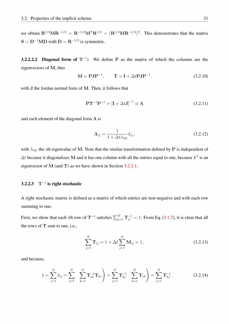
3.2. Properties of the implicit scheme 31

we obtain R1/2MR−1/2 = R−1/2MTR1/2 = (R1/2MR−1/2)T. This demonstrates that the matrix

S = D−1MD with D = R−1/2 is symmetric.

3.2.2.2.2 Diagonal form of T−1: We define P as the matrix of which the columns are the

eigenvectors of M, thus

M = PJP−1, T = I + ∆tPJP−1. (3.2.10)

with J the Jordan normal form of M. Then, it follows that

PT−1P−1 = [I + ∆tJ]−1 ≡ Λ (3.2.11)

and each element of the diagonal form Λ is

Λij =1

1 + ∆tλMi

δij , (3.2.12)

with λMi the ith eigenvalue of M. Note that the similar transformation defined by P is independent of

∆t because it diagonalizes M and it has one column with all the entries equal to one, because 1T is an

eigenvector of M (and T) as we have shown in Section 3.2.2.1.

3.2.2.3 T−1 is right stochastic

A right stochastic matrix is defined as a matrix of which entries are non-negative and with each row

summing to one.

First, we show that each ith row of T−1 satisfies∑N

j=1 T−1ij = 1. From Eq. (3.1.7), it is clear that all

the rows of T sum to one, i.e.,

N∑

j=1

Tij = 1 + ∆tN∑

j=1

Mij = 1 , (3.2.13)

and because,

1 =N∑

j=1

δij =N∑

j=1

(N∑

k=1

T−1ik Tkj

)=

N∑

j=1

T−1kj

(N∑

k=1

Tjk

)=

N∑

j=1

T−1kj . (3.2.14)

32 3.2. Properties of the implicit scheme

Furthermore, for any ∆t > 0

Tij < 0 , for i 6= j , (3.2.15)

so T belongs to the group of matrices for which non-diagonal entries are all negative, T ∈ Zn×n.

To prove that the inverse of T is non-negative we use a theorem from Berman and Plemmons (1979)

(see Theorem 2.3, Chapter 6). The theorem states that any matrix that (i) belongs to the group of Zn×n

matrices and (ii) its eigenvalues are all real and positive has a non-negative inverse. Such a matrix

belongs to a very special type of matrices defined as the M-matrices group. Condition (i) follows from

the definition of T (as we mentioned before) and condition (ii) was demonstrated in Section 3.2.2.1

using the Geršgorin circle theorem. Thus we conclude that T−1 is a right stochastic matrix.

3.2.2.4 T−1 is strictly positive

In the previous section we show that T−1 is non-negative, and in this section we prove that none of its

entries is zero, that is a strictly positive matrix.

Theorem 2.7 in chapter 6 from Berman and Plemmons (1979) states that the inverse, T−1, of an

irreducible non-singular M-matrix is strictly positive, i.e., T−1ij > 0 for all i, j ∈ 1 . . . N . Since we

show in Section 3.2.2.3 that T is a nonsingular M-matrix, it only remains to be demonstrated that T is

irreducible.

Theorem 2.7 in chapter 2 from Berman and Plemmons (1979) states that a matrix T is irreducible if and

only if its direct graph, G(T), is strongly connected. G(T) consists of n vertices P1, . . . , Pn, where

an edge leads from Pi to Pj if and only if Tij 6= 0. Furthermore, it is strongly connected if for any

ordered pair (Pi, Pj) of vertices, there exists a path that leads from Pi to Pj . Clearly, if all the species

collide with each other, then Tij 6= 0 for all i, j and G(T) is strongly connected. This statement holds,

even when neglecting direct collisions between species i and j, provided that each species collides with

another (proxy) species k. This is because the path from Pi to Pj is defined through Pk.

The idea behind the demonstration can be better understood via a simple example. We consider a case

with 3 species where in (A) all the species collide against each other, (B) Species 1 collides with species

2 and 3 and vice versa, but species 2 and 3 do not collide, and (C) species 1 collides with species 2 and

3.2. Properties of the implicit scheme 33

3 but without a back reaction (no feedback).

TA =

1 + ∆t (α12 + α13) −∆tα12 −∆tα13

−∆tα21 1 + ∆t (α21 + α23) −∆tα23

−∆tα31 −∆tα32 1 + ∆t (α31 + α32)

,

TB =

1 + ∆t (α12 + α13) −∆tα12 −∆tα13

−∆tα21 1 + ∆tα21 0

−∆tα31 0 1 + ∆tα31

,

TC =

1 + ∆t (α12 + α13) −∆tα12 −∆tα13

−∆tα21 1 + ∆tα21 0

0 0 1

. (3.2.16)

Figure 3.2.2 shows the corresponding graphs for the cases (A), (B) and (C). In the case (A) all the

vertices are connected because Tij 6= 0 for all i, j. In the case (B), because there are no collisions

between species-2 and species-3 the vertices P2 and P3 are not directly connected, but it is still possible

to move from P2 to P3 through P1, thus the graph of TB is strongly connected. Removing the back

reaction of species 1 onto species 3 from the case B makes it impossible to move from P3 to P1, thus

the graph of TC is not strongly connected and TC is not irreducible.

P1

P3P2

P1

P3P2

P1

P3P2

A B C

Figure 3.2.2: Graphs of the matrices TA, TB and TC

3.2.2.5 Asymptotic stability

The implicit scheme defined by Eq. (3.1.5) is asymptotically stable. This is,

(a) limn→∞

T−nV0k − c = 0 and (b) lim

∆t→∞T−1Vn

k − c = 0 , (3.2.17)

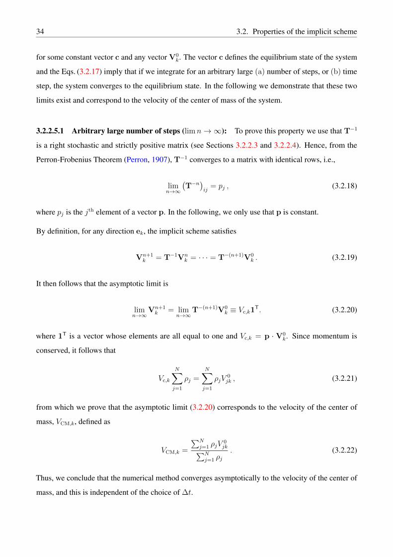
34 3.2. Properties of the implicit scheme

for some constant vector c and any vector V0k. The vector c defines the equilibrium state of the system

and the Eqs. (3.2.17) imply that if we integrate for an arbitrary large (a) number of steps, or (b) time

step, the system converges to the equilibrium state. In the following we demonstrate that these two

limits exist and correspond to the velocity of the center of mass of the system.

3.2.2.5.1 Arbitrary large number of steps (limn→∞): To prove this property we use that T−1

is a right stochastic and strictly positive matrix (see Sections 3.2.2.3 and 3.2.2.4). Hence, from the

Perron-Frobenius Theorem (Perron, 1907), T−1 converges to a matrix with identical rows, i.e.,

limn→∞

(T−n

)ij

= pj , (3.2.18)

where pj is the jth element of a vector p. In the following, we only use that p is constant.

By definition, for any direction ek, the implicit scheme satisfies

Vn+1k = T−1Vn

k = · · · = T−(n+1)V0k . (3.2.19)

It then follows that the asymptotic limit is

limn→∞

Vn+1k = lim

n→∞T−(n+1)V0

k ≡ Vc,k1T. (3.2.20)

where 1T is a vector whose elements are all equal to one and Vc,k = p · V0k. Since momentum is

conserved, it follows that

Vc,k

N∑

j=1

ρj =N∑

j=1

ρjV0jk , (3.2.21)

from which we prove that the asymptotic limit (3.2.20) corresponds to the velocity of the center of

mass, VCM,k, defined as

VCM,k =

∑Nj=1 ρjV

0jk∑N

j=1 ρj. (3.2.22)

Thus, we conclude that the numerical method converges asymptotically to the velocity of the center of

mass, and this is independent of the choice of ∆t.

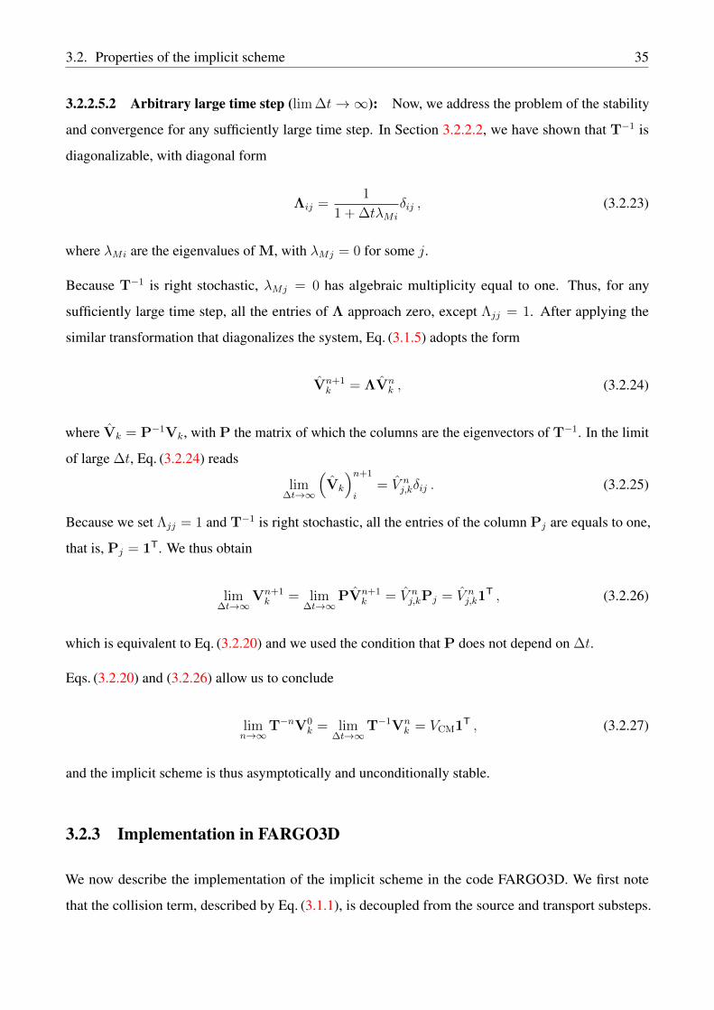
3.2. Properties of the implicit scheme 35

3.2.2.5.2 Arbitrary large time step (lim ∆t→∞): Now, we address the problem of the stability

and convergence for any sufficiently large time step. In Section 3.2.2.2, we have shown that T−1 is

diagonalizable, with diagonal form

Λij =1

1 + ∆tλMi

δij , (3.2.23)

where λMi are the eigenvalues of M, with λMj = 0 for some j.

Because T−1 is right stochastic, λMj = 0 has algebraic multiplicity equal to one. Thus, for any

sufficiently large time step, all the entries of Λ approach zero, except Λjj = 1. After applying the

similar transformation that diagonalizes the system, Eq. (3.1.5) adopts the form

Vn+1k = ΛVn

k , (3.2.24)

where Vk = P−1Vk, with P the matrix of which the columns are the eigenvectors of T−1. In the limit

of large ∆t, Eq. (3.2.24) reads

lim∆t→∞

(Vk

)n+1

i= V n

j,kδij . (3.2.25)

Because we set Λjj = 1 and T−1 is right stochastic, all the entries of the column Pj are equals to one,

that is, Pj = 1T. We thus obtain

lim∆t→∞

Vn+1k = lim

∆t→∞PVn+1

k = V nj,kPj = V n

j,k1T , (3.2.26)

which is equivalent to Eq. (3.2.20) and we used the condition that P does not depend on ∆t.

Eqs. (3.2.20) and (3.2.26) allow us to conclude

limn→∞

T−nV0k = lim

∆t→∞T−1Vn

k = VCM1T , (3.2.27)

and the implicit scheme is thus asymptotically and unconditionally stable.

3.2.3 Implementation in FARGO3D

We now describe the implementation of the implicit scheme in the code FARGO3D. We first note

that the collision term, described by Eq. (3.1.1), is decoupled from the source and transport substeps.

36 3.2. Properties of the implicit scheme

Thus, aside from the collisions, we evolve every species according to the same algorithms described in

Benítez-Llambay and Masset (2016).

The implicit scheme for solving the collision term involves an extra substep, in which the velocity

of each species is partially updated according to the Eq. (3.1.5). There are three different options to

place this additional partial update: (i) before the source step, (ii) after the source step and before the

transport step or, (iii) after the transport step. Options (i) and (iii) are equivalent after the first time

step, which we discard because the dust species do not reach the asymptotic limit in the presence of

additional forces. In this case the relative velocity between the dust and gas asymptotes to its terminal

velocity, where the additional forces are in balance with the drag forces. Since in options (i) and (iii)

the drag forces are computed in the absence of additional forces, they cannot correctly reproduce this

limit (Booth et al., 2015). Option (ii) reproduces this limit because evaluating the collision term after

the source term is equivalent to a solution treating both terms together. While not strictly necessary, the

Standard flow

Sources

Transport

Collisions

Collisions/2Yes

No

VS

VC

Vn+1

VnVn+1/2

Vn

Full

tim

e s

tep

Vn+1/2?

Figure 3.2.3: Figure 1 from Benítez-Llambay et al. (2019). Flowchart of our implementation. During ageneric time step ∆t, depending on whether the predictor step is required, we call the collision routineusing a time step ∆t/2, and obtain a partially updated velocity V n+1/2. We then update the velocities bysources and use the output, VS, as input for the collision step. After this, we use the updated velocities,VC, as input for the transport step, from which we obtain the updated velocity, V n+1. The flow thenreturns to the standard flow, from which a full update has been performed.

coupling between the source and collision steps can be improved by adding a predictor step before the

3.2. Properties of the implicit scheme 37

source step. The source step consists of a partial update of the form:

∂v

∂t= S(v) , (3.2.28)

where S are sources that depend on the velocities. In finite differences, the previous equation reads:

vn+1 = vn + ∆tS(v∗) . (3.2.29)

In the standard implementation, we assume v∗ = vn. However, we can improve the coupling between

collision and source steps by setting v∗ = vn+1/2, i.e., by estimating an advanced velocity from the

collision step with a time step ∆t/2. We then compute the source step using a full time step and finally

calculate the collision step with a full time step.

For completeness, Figure 3.2.3 presents a flowchart of our implementation. During a generic time step,

depending on whether the predictor step is required, the collision routine is called using a time step

∆t/2 and calculates a partially updated velocity. Then, the codes updates the velocities of all the species

by the standard source terms and uses the updated velocities as input for the collision step. During

this step, the code solves Eq. (3.1.5) and then uses the updated velocities as input for the transport step.

After the transport step, a full update has been performed.

∇ Φ

∇ P

INPUTFLUID 2

INPUTFLUID 1 OUTPUT

FLUID 1

OUTPUTFLUID 2

Sources

Sources

Collisions

Transport

Transport

∇ Φ

Figure 3.2.4: Schematic representation of the splitting in FARGO3D including the collision module.

38 3.2. Properties of the implicit scheme

3.2.3.1 Convergence to the correct asymptotic equilibrium

A system of multiple species that exchange momentum due to their velocity difference converges to

an equilibrium state where, in absence of any external acceleration, the relative velocities are zero. To

illustrate this property and to explain why the operator splitting satisfies this condition we consider

a 1D system of N species, each of them experiencing an external acceleration, a, that we assume ot

be independent of the velocity as well as the collision rate, αij . Neglecting the advection term, the

momentum equation of the species j reads as

∂vj∂t

= − 1

ρi

N∑

j=1

αij(vi − vj) + aj , (3.2.30)

which is the analytical form of the equation that is solved between the source and collisions step.

The system can be arranged into a matrix form as

∂tV + MV = A , (3.2.31)

with V = (v1, . . . , vn) and A = (a1, . . . , an), and M being the matrix defined in Eq. (3.1.7). Because

M is similar to a diagonal form, J, (see Section 3.2.2.2) the system can be decoupled, and for each

λMj 6= 0 we have

vj =1

λMj

(aj + cje

−λMjt), (3.2.32)

with vj and aj being the j-component of the vectors P−1V and P−1A, respectively. The unique case

with λMi = 0 gives

vi = ait+ ci. (3.2.33)

The constants defined as c are determined by the initial condition. The solution in the diagonal space

can be written as

V =

(1

λM0

(a0 + c0e

−λM0t), . . . , ait+ ci, . . . ,

1

λMN

(aN + cNe

−λMN t))

. (3.2.34)

After applying the transformation V = PV, and using the fact that the ith column of P is equal to 1T,

3.2. Properties of the implicit scheme 39

each species has a velocity of the form

vk = ait+ ci +N∑

j=1,j 6=iPkj

1

λMj

(aj + cje

−λMjt). (3.2.35)

In the limit of t → ∞ all the velocities go to the limit vk → ait + ci +∑N

j=1,j 6=i Pkj1

λMjaj and the

velocity difference reads as

limt→∞

vk+1 − vk =N∑

j=1,j 6=i(Pk+1j −Pkj)

(P−1A)jλMj

, (3.2.36)

which is zero in absence of any acceleration a.

In the simple case where only two species are considered this equation transform into

limt→∞

v1 − v2 = λ−1(a1 − a2). (3.2.37)

The same limit obtained in Eq. (3.2.36) can be obtained when combining the source step (with an

explicit integration) and the collision step (with the implicit update for the velocity 3.1.2).

Using the same notations as before, but in a discretized case where n indicates a time step, a full update

reads as

Vn+s = Vn + ∆tAn ,

Vn+1 = T−1Vn+s , (3.2.38)

where Vn+s are the updated velocities after the source step. Using the properties studied in Section

3.2.2.2 the velocities in the diagonal space satisfy

Vn+1 =

(1

1 + ∆tλM0

(vn0 + ∆tan0 ), . . . , vni + ∆tani , . . . ,1

1 + ∆tλMN

(vnN + ∆tanN)

), (3.2.39)

where we assumed that λMi = 0. Applying the transformation Vn+1 = PVn+1, each velocity can be

written as

vn+1k = vni + ∆tani +

N∑

j=1,j 6=iPkj

1

1 + ∆tλMj

(vnj + ∆tanj ) , (3.2.40)

40 3.2. Properties of the implicit scheme

which in the limit of ∆t→∞ gives

lim∆t→∞

vn+1k+1 − vn+1

k =N∑

j=1,j 6=i(Pk+1j −Pkj)

(PAn)jλMj

, (3.2.41)

which is the discretized form of Eq. (3.2.36). In the simple case of considering only two species this

reduces to

lim∆t→∞

vn+11 − vn+1

2 = λ−1 (an1 − an2 ) . (3.2.42)

3.2.4 Numerical tests

In this section, we discuss a part of the test suite presented in Benítez-Llambay et al. (2019). We

use these tests to validate the accuracy, convergence properties and robustness of the method and

implementation described in Sections 3.1 and 3.2.3. In all the following tests, the numerical solutions

were obtained using a Courant-Friedrichs-Lewy (CFL) factor of 0.44 (Benítez-Llambay and Masset,

2016), unless a different value is specified.

3.2.4.1 Time evolution of a set of colliding species

When a set of N species evolves under the sole effect of the collision term, simple asymptotically

convergent analytical solutions can be found. This simple test problem validates the correct

implementation of the matrix solver and, at the same time, illustrates the convergence property described

in Section 3.2.2.5.

As a first step, we show the steady-state solution of the problem, which gives insight into the fundamental

property of the physical system, that is, the convergence of all the velocities towards the velocity of

the center of mass. In Section 3.2.2.5, we have already shown that the implicit scheme satisfies this

condition.

The steady-state momentum equation for a set of N species reduces to the matrix equation when

considering only the drag force,

MVk = 0 . (3.2.43)

Because the matrix M, defined by Eq. (3.1.7), is singular (see Appendix 3.2.2.1), the system described

by Eq. (3.2.43) admits a non-trivial solution. By direct calculation it can be shown that the (i, j)-element

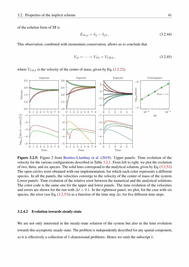
3.2. Properties of the implicit scheme 41

of the echelon form of M is

EM,ij = δij − δjN , (3.2.44)

This observation, combined with momentum conservation, allows us to conclude that

V1k = · · · = VNk = VCM,k , (3.2.45)

where VCM,k is the velocity of the center of mass, given by Eq. (3.2.22).

0 1 2 3 4 5 6 7 80.5

1.0

1.5

2.0

2.5

Vel

oci

ty

2 species

0 1 2 3 4 5 6 7 81.0

1.5

2.0

2.5

3.03 species

0 1 2 3 4 5

−4

−2

0

2

6 species

10−2 10−1

∆t

−4

−2

log

10(e

rror)

Slope = 1.0

Convergence

0 1 2 3 4 5 6 7 8

Time

−5

−4

−3

−2

−1

log

10

( |∆v/(v

+m

in(v

0 j)|)

0 1 2 3 4 5 6 7 8

Time

−5

−4

−3

−2

−1

0 1 2 3 4 5

Time

−5

−4

−3

−2

−1

Figure 3.2.5: Figure 2 from Benítez-Llambay et al. (2019). Upper panels: Time evolution of thevelocity for the various configurations described in Table 3.2.1. From left to right, we plot the evolutionof two, three, and six species. The solid lines correspond to the analytical solution, given by Eq. (3.2.51).The open circles were obtained with our implementation, for which each color represents a differentspecies. In all the panels, the velocities converge to the velocity of the center of mass of the system.Lower panels: Time evolution of the relative error between the numerical and the analytical solutions.The color code is the same one for the upper and lower panels. The time evolution of the velocitiesand errors are shown for the run with ∆t = 0.1. In the rightmost panel, we plot, for the case with sixspecies, the error (see Eq. (3.2.53)) as a function of the time step ∆t, for five different time steps.

3.2.4.2 Evolution towards steady-state

We are not only interested in the steady-state solution of the system but also in the time evolution

towards this asymptotic steady-state. The problem is independently described for any spatial component,

so it is effectively a collection of 1-dimensional problems. Hence we omit the subscript k.

42 3.2. Properties of the implicit scheme

The temporal evolution of the system is described by the solution of

∂V

∂t+ MV = 0 . (3.2.46)

Without loss of generality, by expressing the solution of Eq. (3.2.46) as V(t) =∑

j Vje−λjt, it reduces

to the eigenvalue problem

MVj = λjVj . (3.2.47)

For simplicity, we define the collision rate αij ≡ α0 for i > j and αij = ρj/ρiα0 for i < j, such that

condition (2.1.5) is satisfied.

Defining the function

ζj =N∑

m=j+1

ρm , (3.2.48)

the eigenvalues of M adopt the expression

λj<N = α0

(j +

ζjρj

),

λN = 0 ,

(3.2.49)

with associated eigenvectors

Vj<N = ej −1

ζj

N−1∑

m=j+1

ρm−1em ,

VN =N∑

k=1

ek .

(3.2.50)

Thus, the solution reads

vj<N(t) = −j−1∑

k=1

ρkckζk

e−λkt + cje−λjt + cN ,

vN(t) = −N−1∑

k=1

ρkckζk

e−λkt + cN ,

(3.2.51)

where the coefficients cj are

cj<N = v0j − VCM +

j−1∑

k=1

ρkckζk

,

cN = VCM .

(3.2.52)

3.2. Properties of the implicit scheme 43

3.2.4.3 Numerical solution

Table 3.2.1: Initial density, velocity, eigenvalues and coefficients needed to compute the solution ofEq. (3.2.51). In all the cases we set α0 = 10−1.

j ρj v0j λj cj

Two fluids1 0.2 1.0 0.6000000 -0.83000002 1.0 2.0 0.0000000 1.8333333

Three fluids1 0.2 1.0 1.5000000 -1.53333332 1.0 2.0 0.3800000 -0.64285713 1.8 3.0 0.0000000 2.5333333

Six fluids1 1.0 -1.0 1.3500000 -0.19259262 1.5 2.0 0.9333333 2.79200003 2.0 3.1 0.7500000 4.27272734 2.5 -2.5 0.6600000 -0.37777785 3.0 0.5 0.6166667 2.47692316 3.5 -4.1 0.0000000 -0.8074074

We compare the analytical solution found in Section 3.2.4.2 with the numerical solution obtained by

solving the problem using the implicit scheme. We study the problem with two, three, and six different

species. In order to do this, we set the initial condition on a 1D grid with 16 evenly distributed cells,

over a periodic domain. We note, however, that this choice is arbitrary and, in practice, irrelevant.

This is because the solution does not depend on spatial coordinates. The initial density, velocity,

eigenvalues, and coefficients needed to compute both the numerical and analytical solutions for each

run are summarized in Table 3.2.1. In all the cases, we set the collision rate α0 = 10−1.

The first three panels of Figure 3.2.5 (from left to right) show the time evolution of the velocities. Each

panel corresponds to a different configuration, as listed in Table 3.2.1. The lower panels Figure 3.2.5,

present the relative error of the velocity for all the species, for the corresponding case on top. The time

evolution of the error shows the asymptotic convergence demonstrated in Section 3.2.3.1. Regardless of

the number of species, there is an excellent agreement between the analytical and numerical solutions.

3.2.4.4 Convergence with time step

For the case of six fluids, we additionally check expected first-order convergence rate in time of the

implicit scheme. For this test, we performed five identical runs, in which we progressively decreased

44 3.2. Properties of the implicit scheme

the time step by factors of 2, starting with ∆t = 0.1. The rightmost panel of Figure 3.2.5, displays the

error as a function of the time step, defined as

error(∆t) =

(N∑

j=1

〈v∆tj (t)− vj(t)〉2

)1/2

, (3.2.53)

where 〈〉 denotes the time-average. As expected, the convergence is consistent with a first-order method,

i.e., linear convergence with a slope equal to one.

3.2.4.5 Non-linear drag force

In some regimes, the collision rate might depend on the relative velocity between species, ∆v. In these

cases,Eqs. (3.1.1) become non-linear in the velocities. In principle, the implicit scheme described by

Eq. (3.1.2) can not be used to update the velocities, since it assumes a linear velocity dependency of the

drag force. However, tn the following we present simple tests of an approximation that allows us to

circumvent this issue, which consists in assuming the system to be linear in ∆vn+1, and the collision

rate, αn, to be dependent on ∆vn. This approximation makes it possible for all the properties of the

implicit scheme hold even in the non-linear drag regime. By means of a simple example, we show that

this method is good enough to recover the solution of Eqs. (3.1.1) in the non-linear regime. For this test

we adopt the three different collision rates presented in the Table 3.2.2.

Table 3.2.2: Collision rate α, for the different non-linear drag force laws shown in Fig 3.2.6. Thecoefficients γ, γq, γp, γm and bm are all fixed to unity for the purpose of this test.

Linear Quadratic Power-law Mixedγ γq|∆v| γp|∆v|1/p γm

√1 + bm|∆v|2

We write the analytic solutions of the non-linear drag force regime. We consider two species with

initial densities and velocities, ρ1 = ρ2 = 1 and v1 = 20, v2 = 10, respectively, and obtain numerical

solutions following Section 3.2.4.1. To this end the drag coefficient α ≡ α(|∆v|), with ∆v = v1− v2.

The system of equations transform into

∂tv1 = −α(|∆v|)(v1 − v2) , (3.2.54)

∂tv2 = −α(|∆v|)(v2 − v1) , (3.2.55)

3.3. Damping of a sound wave 45

Table 3.2.2 shows all the collision rates that we explored, where for the power-law regime we set the

index p = 2.

Table 3.2.3: Analytical solution for the different non-linear drag force laws shown in Fig 3.2.6.

Linear Quadratic Power-law Mixed∆v

∆v0

e−γt (2γqt|∆v0|+ 1)−1(√|∆v0|γ2t+ 1

)−2 −2f(t)

∆v20bmf(t)2 − 1

with f(t) =e−2γmt

√bm∆v2

0 + 1 + 1.

0.0 0.5 1.0 1.5 2.0

Time

10

12

14

16

18

20

Vel

oci

ty

Quadratic

Gas1

Gas2

Linear drag

0.0 0.5 1.0 1.5 2.0

Time

10

12

14

16

18

20

Power-law

0.0 0.5 1.0 1.5 2.0

Time

10

12

14

16

18

20

Mixed

Figure 3.2.6: Figure 12 from Benítez-Llambay et al. (2019). Analytical (solid lines) and numerical(open circles) solutions for a quadratic (left panel), power law with p = 2 (center panel) and mixed(right panel) drag forces. The dashed line is the solution for a linear drag force.

Each panel of Figure 3.2.6 shows the analytical and numerical solutions, with solid lines and open

circles, respectively. The dashed lines correspond to the solution obtained for a linear drag force. In all

the non-linear drag regimes, the agreement between the analytical and numerical solutions is excellent.

3.3 Damping of a sound wave

Sound waves are a natural outcome of the fluid equations when pressure perturbations are considered.

Dust fluids, however, cannot support sound waves. In systems composed of gas and dust species, sound

waves can propagate – supported by the gas component – but their properties are modified due to the

momentum exchange with the dust. Solutions for the case of one gas and one dust species were found

by Laibe and Price (2012), who showed that sound waves are damped by the effect of the collision

46 3.3. Damping of a sound wave

Figure 3.3.1: Figure 3 from Benítez-Llambay et al. (2019). Numerical (open circles) and analytical(solid lines) solutions of the test described in Section 3.3 for the configurations listed in Table 3.3.1.We plot the time evolution of the normalized velocity (upper panels) and density (lower panels). Theresults for one and four dust species are shown in the left and right panels, respectively. The bluecircles correspond to the gas, while the other colors correspond to the dust species. All the solutionswere obtained at x = 0. The normalized density and velocity are defined as δρ/(Aρ0) and δv/(Acs),respectively, with A = 10−4.

between dust and gas. Solving this problem is relevant since it provides a direct – and perhaps the

simplest – way to test the coupling between the implicit solver and the transport and source steps.

In the following, we derive the dispersion relation for the general problem of one gas and N − 1 dust

species which, together with the general expression for the eigenvectors, allows us to find the full

solution to the problem.

3.3. Damping of a sound wave 47

Table 3.3.1: Initial conditions for the damping of the sound wave test.

j ρj δρj δvj tsj ωTwo species

g 1.000000 1.000000 −0.701960− 0.304924i – 1.915896− 4.410541i1 2.240000 0.165251− 1.247801i −0.221645 + 0.368534i 0.4

Five speciesg 1.000000 1.000000 −0.874365− 0.145215i – 0.912414− 5.493800i1 0.100000 0.080588− 0.048719i −0.775380 + 0.308952i 0.1000002 0.233333 0.091607− 0.134955i −0.427268 + 0.448704i 0.2154433 0.366667 0.030927− 0.136799i −0.127928 + 0.313967i 0.4641594 0.500000 0.001451− 0.090989i −0.028963 + 0.158693i 1.000000

3.3.1 Dispersion relation and eigenvectors

We now derive the dispersion relation for the case of one gas and N − 1 dust species and find the

general eigenvectors of the problem. For that, we assume that the gas pressure is given by P = c2sρg,

with a constant sound speed, cs, and define the collision rate between the gas and dust species following

Eq. (2.1.6), with αj = t−1sj , where tsj is the stopping time.

Assuming solutions of the form ρj = ρ0j + δρj and vj = δvj , with ρ0

j constant, and neglecting quadratic

terms in the perturbations, the continuity and momentum equations for the gas and dust species become

∂δρg

∂t+ ρ0

g

∂δvg

∂x= 0 , (3.3.1)

∂δρj∂t

+ ρ0j

∂δvj∂x

= 0 , (3.3.2)

∂δvg

∂t+

N−1∑

m=1

ε0mtsm

(δvg − δvm) +c2

s

ρ0g

∂δρg

∂x= 0 , (3.3.3)

∂δvj∂t

+1

tsj(δvj − δvg) = 0, (3.3.4)

where j = 1, ..., N − 1 is the index of the dust species.

We first note that the momentum equation is decoupled from the continuity equation for dust species, so

the order of the problem is effectively reduced from 2N to N + 1. Without loss of generality, we write

any perturbation δf as δf = δfeikx−ωt, with k a real wavenumber. Thus, from Eqs. (3.3.1)-(3.3.4), we

obtain the dispersion relation

F (ω, ωs) ≡ ω2

(1 +

N−1∑

m=1

εm1− ωtsm

)+ ω2

s = 0 , (3.3.5)

48 3.3. Damping of a sound wave

with ωs = kcs. The singular values ωm = t−1sm correspond to δvg = 0, δρg = 0, so are not considered.

Finally, the components of the associated eigenvectors are

δvg

cs

= −i ωωs

δρg

ρ0g

, (3.3.6)

δvjcs

= −i ωωs

1

(1− ωtsj)δρg

ρ0g

, (3.3.7)

δρjρ0j

=1

1− ωtsjδρg

ρ0g

, (3.3.8)

for any δρg, which completes the solution of the problem.

3.3.2 Eigenvalues for the sound wave test problem

Eq. (3.3.5) can be written as a polynomial equation of degree N + 1. In the following, we show that

at least N − 1 roots of (3.3.5) are real and positive and are thus associated with pure damping. We

furthermore identify the intervals in which they can be found. This allows a simple bisection algorithm

to be used to find them. We additionally explain how to use Vieta’s formulae to find the final two roots

which are, in general, complex. These two complex roots are the most interesting ones since they

describe the propagation of damped sound waves. To solve the dispersion relation (3.3.5), we write it

as the polynomial equation

P (ω) = ωN+1 + aNωN + . . .+ a0 = 0 . (3.3.9)

The N + 1 roots of (3.3.9) are the eigenvalues of the problem. The polynomial P has at least N − 1

real positive roots. This is proven by first noticing that F is positive for ω < min (t−1sm). Since tsm > 0,

no real root exists for ω < 0. In addition, the one-sided limits of F satisfy

limω→t−1±

sm

F (ω, ωs) = ±∞ , (3.3.10)

i.e., the function changes sign at each side of the singular points, from which we conclude that there

is at least one real positive root between two adjacent singular points, giving N − 2 positive roots.

3.3. Damping of a sound wave 49

Furthermore, since

limω→∞

F (ω, ωs) =∞ , (3.3.11)

there is at least one more positive root beyond the last singular point. All of these roots correspond to

pure damping solutions.

An upper bound for the largest real root can be found. Defining t−1sN−1 as the largest singular point, for

ω t−1sN−1, yields f > 0 if

1 +N−1∑

m=1

εm1− ωtsm

' 1− 1

ω

N−2∑

m=1

εmtsm

+εN−1

1− ωtsN−1

> 0 . (3.3.12)

This expression is equivalent to the quadratic inequality

− tsN−1ω2 +

[1 + εN−1 + tsN−1

N−2∑

m=1

εmtsm

]ω −

N−2∑

m=1

εmtsm

> 0 , (3.3.13)

from which we find that the largest positive root of P is smaller than the largest root of Eq. (3.3.13).

Having found the N − 1 roots of P , ω1, . . . , ωN−1, we can use Vieta’s formulae to find the remaining

roots ωN and ωN+1

ωNωN+1 = (−1)N+1 a0

N−1∏

j=1

ω−1j , (3.3.14)

ωN + ωN+1 = −aN −N−1∑

j=1

ωj . (3.3.15)

where a0, aN satisfy

a0 = (−1)N−1 ω2s

N−1∏

j=1

t−1sj , (3.3.16)

aN = −N−1∑

j=1

t−1sj (1 + εj) . (3.3.17)

Eqs. (3.3.14) and (3.3.15) can be written as a second order polynomial equation, from which we obtain

the final two roots, which are in general complex and the most interesting ones because they lead to the

50 3.3. Damping of a sound wave

propagation of the wave.

Figure 3.3.2: Example of the real roots of F (ω, ωs) for a case with two dust species with ts = 0.5,ε1 = 0.1, and ts = 1, ε2 = 10. The dashed lines shows the singularities at ω = 1/ts. Orange circlescorrespond to the two damping rates and ωs = 2π.

3.3.3 Numerical solution

Using the eigenstates as initial condition we obtain the numerical solutions for the oscillatory damped

modes. From the two possible oscillatory modes, we choose only one because the other one is the

complex conjugate, producing the same solution but propagating in the opposite direction. We do

not consider the solutions that correspond to perfect damping because they behave as those studied in

Section 3.2.4.1.

We study the cases of one gas fluid combined with one and four dust species, respectively. As initial

condition we set a zero background velocity, constant background density, ρ0j , and perturbations, δf , of

the form

δf = A[Re(δf)

cos(kx)− Im(δf)

sin(kx)], (3.3.18)

where A is a small amplitude needed to ensure linearity. We set its value to 10−4cs and 10−4ρ0g for the

velocity and density perturbations, respectively, and set cs = 1. The background densities, perturbation

amplitudes, stopping times, and complex eigenvalue for each case are listed in Table 3.3.1. We consider

a domain of size L = 1, with spatial coordinate x ∈ [0, L], split into 103 evenly spaced grid cells. We

3.3. Damping of a sound wave 51

Figure 3.3.3: Figure 3 from Benítez-Llambay et al. (2019). Numerical (circles) and analytical (solidlines) imaginary and real part of the eigenvalue ω, as a function of the stopping time ts, obtained for thetwo-fluid case described in Table 3.3.1. The dashed line corresponds to the time step ∆t = 1.375×10−2,which is fixed for all the runs.

consider the wavenumber k = 2π/L and set periodic boundary conditions.

Figure 3.3.1 shows the analytical (solid lines) and numerical (open circles) solutions, measured at x = 0

for the two considered configurations. The solution corresponding to different species is plotted with a

different color. The first column shows the solution obtained for one gas and one dust species, while the

second one shows the same for the case of five, one gas and four dust, species. In the upper and lower

panels we plot the normalized velocity, defined as δv/(csA) and the normalized density, defined as

δρ/(ρA), respectively. From Figure 3.3.1, it is clear that the analytical solution is successfully recovered

by our implementation. This test validates the coupling of the drag force in combination with the source

and transport steps for a wide range of stopping times.

To study the coupling of the implicit scheme with the transport and source steps in a more challenging

situation, we test the damping of a sound wave for a range of stopping times 10−4 ≤ ts ≤ 10 and a fixed

time step, such that we test both stiff and non-stiff regimes for the collisions. We consider the two-fluid

problem described in Table 3.3.1, for different stopping times. We use a domain of size L = 1 and 32

cells, which sets a time step ∆t = 1.375× 10−2, given by the standard CFL condition of FARGO3D.

For stopping times smaller than the time step the regime becomes more and more stiff. Note that,

because of the CFL condition, the degree of stiffness depends on the resolution. We integrate the system

until it reaches a final time t = 10. We measure the damping rate, Re(ω), and the oscillatory frequency,

Im(ω) by fitting the numerical solutions. The upper and lower panels of Figure 3.3.3 show the analytical

frequency and damping rate, respectively, together with the measurements from our simulations.

The error of the implicit scheme converges to zero asymptotically with ∆t (see Section 3.2.2). Therefore,

52 3.4. Steady-state, first-order drift solutions

for a fixed time step, the smaller the stopping time is, the stiffer the regime is and the faster the errors

are damped. Furthermore, the excellent agreement of the oscillatory frequency permits to conclude that

no phase-error is introduced by the implicit scheme, in the operator splitting approximation.

3.4 Steady-state, first-order drift solutions

In this section, we present the analytical solution of the steady-state radial drift for an arbitrary number

of species, to first-order in the velocities with respect to an exact background. We then compare

this analytical solution with the numerical one. The background is obtained by considering pressure

gradients (which are not necessarily small) and neglecting drag forces between species. This solution

generalizes that obtained by Nakagawa et al. (1986a), who presented a self-consistent first-order solution

with respect to a Keplerian background for a disk, composed of gas- and one dust-species. In their

approach, the background flow is obtained as the solution of the vertically integrated disk-equations

when neglecting pressure and drag forces. This assumption implies that both the radial pressure gradient

and the drag force are small perturbations that can be added linearly to the Keplerian velocity. However,

the assumption of a small pressure gradient is not strictly necessary to find a background solution.

This generalization provides us with improved steady-state disk models which will allow us to

thoroughly test our numerical method.

3.4.1 Generalized steady-state drift solutions

We consider a vertical integrated and axisymmetric disk in steady state. We assume a cylindrical

coordinate system and an isothermal equation of state. The surface density, Σ, is the vertically

integrated density, Σ =∫∞−∞ ρ(r, z)dz, and the vertically integrated pressure is P = c2

sΣ, with cs the

sound speed. The gravitational potential is Φ = −GM/r, hence ∂rΦ = v2K/r, with vK the keplerian

velocity. Furthermore, we assume a non-flared disk with constant aspect-ratio h = cs/vK, thus,

∂rP/Σ = c2s/r (dlogP/dlogr) = h2v2

K/r (dlogP/dlogr). Under these assumptions (neglecting the

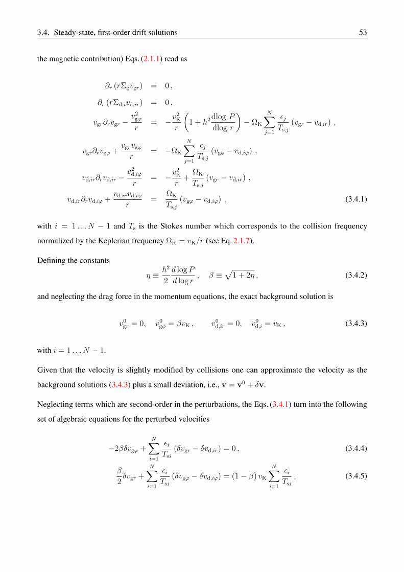
3.4. Steady-state, first-order drift solutions 53

the magnetic contribution) Eqs. (2.1.1) read as

∂r (rΣgvgr) = 0 ,

∂r (rΣd,ivd,ir) = 0 ,

vgr∂rvgr −v2

gϕ

r= −v

2K

r

(1 + h2 dlog P

dlog r

)− ΩK

N∑

j=1

εjTs,j

(vgr − vd,ir) ,

vgr∂rvgϕ +vgrvgϕ

r= −ΩK

N∑

j=1

εjTs,j

(vgφ − vd,iϕ) ,

vd,ir∂rvd,ir −v2

d,iϕ

r= −v

2K

r+

ΩK

Ts,j

(vgr − vd,ir) ,

vd,ir∂rvd,iϕ +vd,irvd,iϕ

r=

ΩK

Ts,j

(vgϕ − vd,iϕ) , (3.4.1)

with i = 1 . . . N − 1 and Ts is the Stokes number which corresponds to the collision frequency

normalized by the Keplerian frequency ΩK = vK/r (see Eq. 2.1.7).

Defining the constants

η ≡ h2

2

d logP

d log r, β ≡

√1 + 2η , (3.4.2)

and neglecting the drag force in the momentum equations, the exact background solution is

v0gr = 0, v0

gφ = βvK , v0d,ir = 0, v0

d,i = vK , (3.4.3)

with i = 1 . . . N − 1.

Given that the velocity is slightly modified by collisions one can approximate the velocity as the

background solutions (3.4.3) plus a small deviation, i.e., v = v0 + δv.

Neglecting terms which are second-order in the perturbations, the Eqs. (3.4.1) turn into the following

set of algebraic equations for the perturbed velocities

−2βδvgϕ +N∑

i=1

εiTsi

(δvgr − δvd,ir) = 0 , (3.4.4)

β

2δvgr +

N∑

i=1

εiTsi

(δvgϕ − δvd,iϕ) = (1− β) vK

N∑

i=1

εiTsi

, (3.4.5)

54 3.4. Steady-state, first-order drift solutions

−2δvd,iϕ +1

Tsi

(δvd,ir − δvgr) = 0 , (3.4.6)

1

2δvd,ir +

1

Tsi

(δvd,iϕ − δvgϕ) =(β − 1) vK

Tsi

, (3.4.7)

for i = 1, . . . , N and where we used that v2ϕ/r ' (v0

ϕ)2/r + 2ΩKβδvϕ and vr∂rvϕ + vrvϕ/r 'δvrβ (∂rvK + ΩK) when neglecting quadratic terms in the perturbed velocity.

From Eqs. (3.4.6) and (3.4.7) we obtain the dust velocities in terms of the gas velocity which, in

combination with Eqs.(3.4.4) and (3.4.5), allow us to find the gas velocity perturbations. Defining

SN ≡N∑

i=1

εi

1 + Ts2i

, QN ≡N∑

i=1

εiTsi

1 + Ts2i

, (3.4.8)

the gas velocity perturbations read

δvgr(r) = −2βQNΨ (β − 1) vK , (3.4.9)

δvgϕ(r) = −[(SN + β)SN +Q2

N

]Ψ (β − 1) vK , (3.4.10)

with Ψ ≡[(SN + β)2 +Q2

N

]−1.

Finally, the expressions for the dust velocity perturbations are

δvd,ir =2Tsi

1 + Ts2i

(β − 1) vK +δvgr + 2Tsiδvgϕ

1 + Ts2i

, (3.4.11)

δvd,iϕ =1

1 + Ts2i

(β − 1) vK +2δvgϕ − Tsiδvgr

2(1 + Ts

2i

) . (3.4.12)

The velocities given by Eqs. (3.4.9) and (3.4.12) are solution only if they satisfy the continuity equations.

In our case we are assuming a non-flared disk2 and the perturbed velocities are proportional to the

Keplerian velocity, thus, the continuity equations

∂r(rΣ0

gδvgr

)= 0 , (3.4.13)

∂r(rΣ0

d,iδvd,ir

)= 0 , (3.4.14)

2Flared disks might not be solved in this formalism because momentum and continuity equation impose conditions onthe radial velocity that are non consistent, in other words, the problem is over-determined.

3.4. Steady-state, first-order drift solutions 55

are satisfied for power-law background surface-density profiles with exponent d log Σ/d log r = −1/2.

When considering only one dust species and h 1, we can write β ' 1 + η and Eqs. (3.4.9) – (3.4.12)

are the solution found by Nakagawa et al. (1986a). Dipierro et al. (2018) found a similar solution for an

arbitrary number of species for a viscous disk assuming a Keplerian background. This solution can be

easily improved following our approach.

3.4.2 Radial drift for a particle-size distribution

In this section we present the results obtained when considering different particle-size distributions and

compare with the solution obtained with only one particle size. The distributions follows from the form

described in Section 2.1.2. We consider a disk with h = 0.05 and Σ = Σ0r−1/2AU with Σ0 = 1. The units

are such GM = 1. Because we assume a distribution of Stokes numbers rather than particle-sizes, we

are implicitly assuming that the sizes vary with radius.

The first result is the radial velocity of the gas for different distributions and its comparison to the two-

fluid problem. We then calculate the fraction of particles that are drifting outwards, their corresponding

Stokes numbers and the fraction of the total mass of the distribution that they represent. We adopt four

different slopes, q = 1, 2.5, 3.5, 4 and three dust-to-gas dust density ratio ε = 0.01, 01, 1. For all the

distributions we fixed the minimum Stokes number to Ts,min = 10−4 and we continuously varying the

maximum, Ts,max, from 10−3 up to 10.

Figure 3.4.1 shows the results. The radial drift of the gas is slightly affected by the distribution compared

to the two-fluid drift solution. As the slope increases the peak of the drift-velocity moves to larger

Stokes numbers. Increasing the dust-to-gas density ratio also affects the maximum of the radial velocity.

Distributions with q ∼ 4 have a maximum drift at Stokes numbers larger than unity. Similarly, when

ε > 0.1 the maximum drift moves towards Ts,max = 10.

3.4.3 Numerical solution

We now use the steady-state solution found in the previous section to test our implementation in

the context of PPDs. For this test we initialize a large-scale 1-dimensional disk using the first-order

steady-state solutions, given by Eqs. (3.4.9)-(3.4.12). The computational domain spans from r = 1 to

r = 100, evenly spaced in a logarithmic grid over 1024 points. We assume an isothermal equation of

56 3.4. Steady-state, first-order drift solutions

10−7

10−6

10−5

10−4

10−3

10−2

vgr/c s

ε = 0.01

two-fluid

q = 1

q = 2.5

q = 3.5

q = 4

ε = 0.1 ε = 1

0.0

0.2

0.4

0.6

0.8

1.0

Nout/N

q = 1

q = 2.5

q = 3.5

q = 4

10−4

10−3

10−2

10−1

100

max(T

s,out)

q = 1

q = 2.5

q = 3.5

q = 4

10−3 10−2 10−1 100 101

Ts,max

0.0

0.2

0.4

0.6

ε out/ε

q = 1

q = 2.5

q = 3.5

q = 4

10−3 10−2 10−1 100 101

Ts,max

10−3 10−2 10−1 100 101

Ts,max

Figure 3.4.1: From top to bottom: The panels in the first-row show the radial velocity of the gas as afunction of the maximum Stokes number of the distribution. The dashed line shows the radial velocitywhen only the species with the maximum Stokes number is considered, i.e. the two-fluid problem. Thesecond row shows the fraction of dust-species that are moving outwards (following the gas drift) as afunction of the maximum Stokes number of the distribution. The third row shows the maximum Stokesnumber of all the species that are drifting outwards as a function of the maximum Stokes number ofthe distribution. In all the panels colors correspond to different slopes of the particle-size distribution.The bottom panels show the fraction of the total dust-to-gas density ratio that is moving outwards. Thevalues are obtained at r = 10AU.

state and set boundary conditions equal to the steady-state solutions for all the species. The absence of

perfect numerical equilibrium at the beginning of the runs produces wave-patterns that propagate in the

3.4. Steady-state, first-order drift solutions 57

disk and reach the boundaries of the mesh. To remove these spurious waves from the active domain we

use small damping zones close to the boundaries (de Val-Borro et al., 2006). These buffers extend over

a region such that ∆Ω = 0.1 for both the inner and outer buffers (see Benítez-Llambay et al., 2016),

and the damping rate is set to one third of the local Keplerian frequency. We only damp the density and

radial velocity to the value given by the initial condition.

We consider two cases with two species and two cases with four species, and vary the degree of coupling

between gas and dust species. To test our implementation in more challenging regimes, we furthermore

vary the aspect ratio, h, of the disk, adopting the values h ∈ [0.05, 0.1, 0.15] for each configuration. In

all the cases, we numerically integrate the 1D disks until the steady-state is reached. The initial surface

density of the gas component is not relevant for these tests.

Figure 3.4.2 displays the radial velocities for all the cases studied. The results corresponding to different

species and different parameters are shown in each column and row, respectively. From top to bottom,

the first two rows, show the radial velocity for the two-fluid configurations and the last two rows the

radial velocities for the test with four fluids. The analytical solutions, given by Eqs. (3.4.9) and (3.4.11),

are plotted with solid lines. The different colors represent different species. Furthermore different

symbols account for different aspects ratios. The parameters corresponding to each species are quoted

inside of the panels. We observe that the agreement between the analytical and numerical solutions

is excellent, and independent of the parameters and the number of species. The tests presented here

validate simultaneously the first-order steady-state disk-drift solution and our numerical implementation.

We note an interesting result from the multiple fluid test. In the two fluids cases it is impossible to revert

the sign of the radial velocity of the dust component due to momentum conservation, but, its magnitude

depends on the dust-to-gas density ratio as well as the degree of coupling to the gas. However, this is

no longer true in the more general case of multiple species. In this case, very well coupled dust can be

transported outwards by the gas (see, for example, the fourth panel of the third row and the second and

third panels of the fourth row). We finally comment that the same level of agreement was observed for

the azimuthal velocity, which is not surprising given that the two directions are coupled.

3.4.3.1 Convergence test

We additionally performed a convergence test with resolution. This test consists in taking one particular

case and measuring the error of the numerical solution when changing the resolution. For this particular

58 3.4. Steady-state, first-order drift solutions

100 101 102

0.0

0.2

0.4

0.6

Rad

ial

Vel

oci

ty×

10

2

Gas

h=0.05

h=0.10

h=0.15

100 101 102

−0.6

−0.4

−0.2

0.0

Ts1 = 1.0ε1 = 1.0

Dust1

100 101 102

0.0

0.2

0.4

0.6

0.8

Rad

ial

Vel

oci

ty×

10

4

100 101 102

−0.8

−0.6

−0.4

−0.2

0.0

Ts1 = 10−2

ε1 = 1.0

100 101 102

0.0

0.2

0.4

0.6

Rad

ial

Vel

oci

ty×

10

3

100 101 102

−6

−4

−2

0

Ts1 = 1.0ε1 = 0.1

100 101 102

−0.6

−0.4

−0.2

0.0

Ts2 = 10−1

ε2 = 0.5

Dust2

100 101 102

0.0

0.1

0.2

0.3

0.4 Ts3 = 10−2

ε3 = 1.0

Dust3

100 101 102

Radius

0.0

0.1

0.2

0.3

0.4

Rad

ial

Vel

oci

ty×

10

2

100 101 102

Radius

0.0

0.1

0.2

0.3

0.4Ts1 = 10−2

ε1 = 0.1

100 101 102

Radius

0.0

0.1

0.2

Ts2 = 10−1

ε2 = 0.5

100 101 102

Radius

−0.4

−0.2

0.0

Ts3 = 1.0ε3 = 1.0

102 103 104

N

10−6

10−5

10−4

Err

or

Slope = -2.2

Figure 3.4.2: Figure 6 from Benítez-Llambay et al. (2019). Analytical (solid lines) and numerical(open colored symbols) solutions for the first-order dust radial drift test problem, described in Section3.4.1. The analytical solutions are given by Eqs. (3.4.9) and (3.4.11). In the smaller panels, we plot theradial velocity for all the cases studied. Different columns correspond to different species (labeled at thetop of each of the uppermost panels) while different rows correspond to runs with different parameters.For each set of parameters, we run the same test with different aspect-ratios, h, and plot the resultingradial velocity with different symbols (see the legend in the leftmost upper panel). The parameters ofeach run are quoted inside of the small panels. In the large panel located at the right upper corner, weadditionally plot the result of the convergence test described in Section 3.4.3.1.

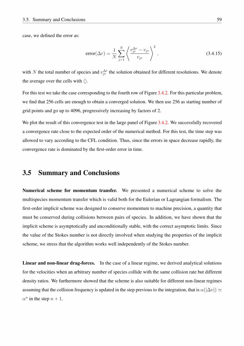
3.5. Summary and Conclusions 59

case, we defined the error as:

error(∆r) =1

N

N∑

j=1

⟨v∆rjr − vjrvjr

⟩2

, (3.4.15)

with N the total number of species and v∆rjr the solution obtained for different resolutions. We denote

the average over the cells with 〈〉.

For this test we take the case corresponding to the fourth row of Figure 3.4.2. For this particular problem,

we find that 256 cells are enough to obtain a converged solution. We then use 256 as starting number of

grid points and go up to 4096, progressively increasing by factors of 2.

We plot the result of this convergence test in the large panel of Figure 3.4.2. We successfully recovered

a convergence rate close to the expected order of the numerical method. For this test, the time step was

allowed to vary according to the CFL condition. Thus, since the errors in space decrease rapidly, the

convergence rate is dominated by the first-order error in time.

3.5 Summary and Conclusions

Numerical scheme for momentum transfer. We presented a numerical scheme to solve the

multispecies momentum transfer which is valid both for the Eulerian or Lagrangian formalism. The

first-order implicit scheme was designed to conserve momentum to machine precision, a quantity that

must be conserved during collisions between pairs of species. In addition, we have shown that the

implicit scheme is asymptotically and unconditionally stable, with the correct asymptotic limits. Since

the value of the Stokes number is not directly involved when studying the properties of the implicit

scheme, we stress that the algorithm works well independently of the Stokes number.

Linear and non-linear drag-forces. In the case of a linear regime, we derived analytical solutions

for the velocities when an arbitrary number of species collide with the same collision rate but different

density ratios. We furthermore showed that the scheme is also suitable for different non-linear regimes

assuming that the collision frequency is updated in the step previous to the integration, that is α(|∆v|) 'αn in the step n+ 1.

60 3.5. Summary and Conclusions

Implementation in FARGO3D. We demonstrate that the operator splitting implementation converges

to the correct equilibrium solution when solving the Collision step between the Source and Transport

steps.

Damping of a sound wave. We derived the dispersion relation that determines the propagation of a

sound wave when a gaseous fluid exchanges momentum with multiple pressureless fluids, e.g., dust

species (neglecting the collisions between pressureless fluids). The benefit of having a closed form of

the dispersion relation — instead of a polynomial of degree N + 1 — is that we could prove that only

two of the N + 1 roots are complex and provide an efficient method to find all the damping rates. We

recovered the analytical solutions with FARGO3D confirming that the implementation converges to

correct equilibrium, even in stiff regimes where the Stokes number is significantly smaller (up to four

orders of magnitude) than the explicit timestep imposed by the CFL condition.

Generalized first-order drift solutions. We obtained first-order, steady-state solutions for the radial

drift of multiple dust species in protoplanetary disks, in which the pressure gradient is not necessarily

small. Using these solutions we have shown that for particle-size distributions a significant fraction

of the dust particles moves outwards, up to 60% for distributions with ε ∼ 1, depending on the slope.

We performed simulations with FARGO3D to validate our implementation of the collision module,

successfully recovering the steady-state solution considering a disk with a radial extension of 100 AU.

4Hall-Dominated Protoplanetary Disks

The importance of the Hall effect in protoplanetary disks has been extensively discussed in the past

two decades by several authors (see e.g. Wardle, 1999; Balbus and Terquem, 2001; Sano and Stone,

2002; Salmeron and Wardle, 2003; Pandey and Wardle, 2008; Wardle and Salmeron, 2012; Bai, 2014).

Detailed calculations of chemical abundances and ionization fractions including chemical reaction

networks have provided an understanding of the relative importance of the Hall effect together with the

Ohmic and ambipolar diffusion (e.g. Salmeron and Wardle, 2008; Bai, 2011a). Furthermore, numerical

simulations provided a new picture of PPDs dynamics enhancing the importance of the Hall effect in

planet forming processes (e.g. Bai, 2014; Lesur et al., 2014; Bai, 2017; Béthune et al., 2017).

In this chapter, we discuss the results presented in Krapp et al. (2018) (including tables and figures),

where we addressed the existence of zonal flows and vortices induced by Hall-MHD turbulence

in protoplanetary disks. We consider vertically unstratified cylindrical disk, including the Ohmic

dissipation and the Hall effect. Such simplification seems adequate to model to regions close to the

midplane of a typical PPD, at inner radii r . 20AU. At these locations, the Hall effect likely dominates

over Ohmic dissipation, and ambipolar diffusion (AD) is thought to be negligible.

We focus here on the discussion of two different regimes that we defined as "Weak" and "Strong" Hall-

regimes. A distinction that follows from a transition that goes from a likely turbulent to a self-organized

state as the Hall diffusion increases and dominates the evolution of the induction equation (Kunz and

Lesur, 2013).

As a first step, we study the Maxwell and Reynolds stresses, analyzing the time evolution of the

dimensionless stress, α, in the context of a globally isothermal PPDs. The results clearly show the effect

of the magnetic field polarity in the turbulent flow due to the inclusion of the Hall effect. We begin the

61

62 4.1. Numerical considerations

discussion by comparing global isothermal disk simulations with the actual results by O’Keeffe and

Downes (2014), obtained in the framework of multifluid MHD, and Béthune et al. (2016), which used a

single-fluid Hall-MHD approach.

Secondly, we study a regime where the Hall effect likely dominates the dynamics and where the

turbulent flow is prone to be organized in large scale coherent structures. This section is a followup of

the previous work of Béthune et al. (2016) that allows us to test our numerical approach, which has

never been used to study such a challenging regime.

Finally, after the numerical validation of our implementations in the non-linear regime, we study the

effect of the self-organization on the dust dynamics, where the dust equations are solved using the

implicit updated discussed in Chapter 3. This study is done assuming a radially varying disk model,

with the additional inclusion of different azimuthal net flux.

4.1 Numerical considerations

In the following, we discuss boundary conditions, resolution requirements, and additional numerical

techniques correctly implemented to simulate PPDs with the Hall effect. In Appendix A.1, we add a

description of the numerical scheme used to solve the induction equation with the Hall term, together

with the corresponding tests.

4.1.1 Cylindrical simulations of PPDs

All the simulations presented in this section are based on an unique setup. We consider a disk with a

central star and assume a cylindrical gravitational potential. We solve the Eqs. (2.1.1) and (2.1.2) in a

cylindrical mesh with vertical, radial and azimuthal extensions defined as Lz, Lr and Lφ, respectively.

The simulatins were performed with FARGO3D and NIRVANA-III and the numerical methods were

discussed in Sections 1.5.1 and 1.5.2.

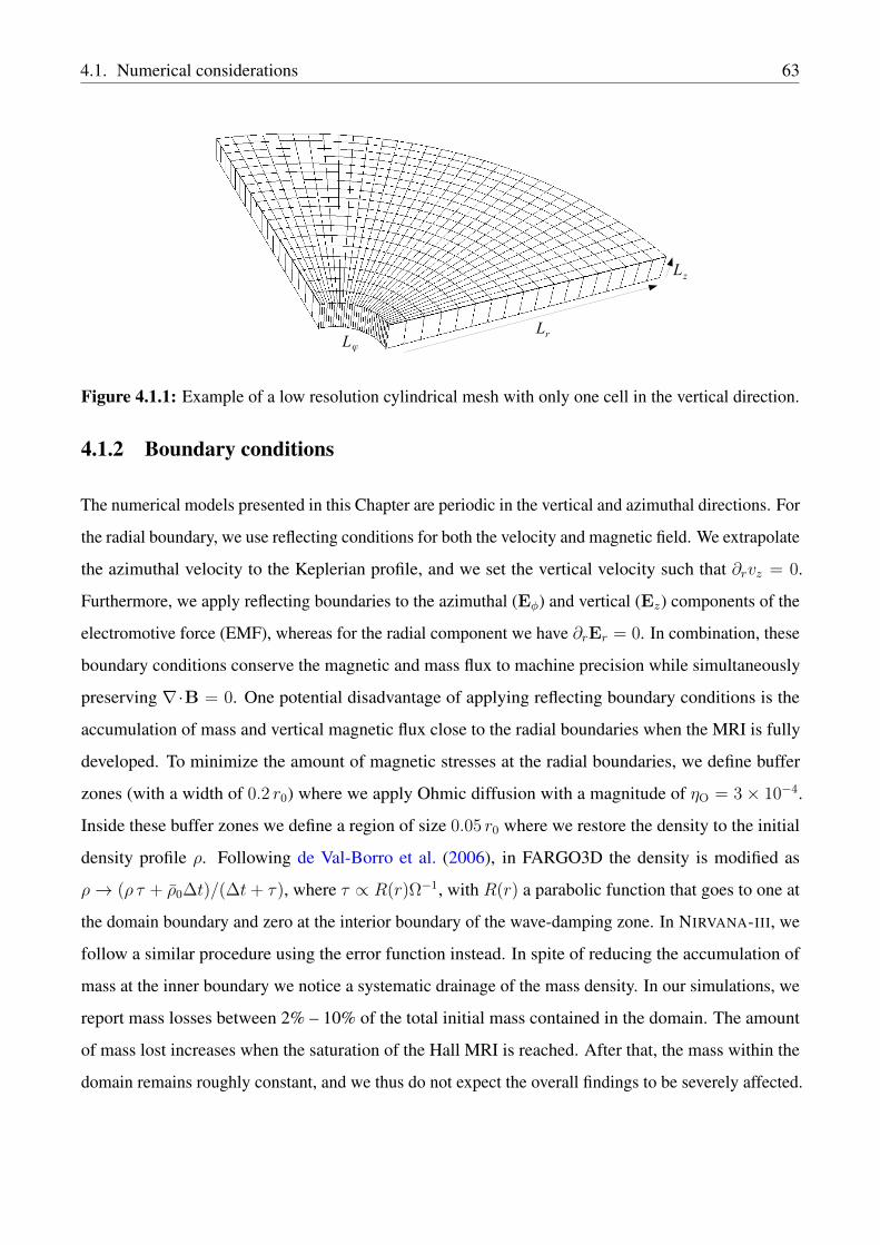
4.1. Numerical considerations 63

LrLφ

Lz

Figure 4.1.1: Example of a low resolution cylindrical mesh with only one cell in the vertical direction.

4.1.2 Boundary conditions

The numerical models presented in this Chapter are periodic in the vertical and azimuthal directions. For

the radial boundary, we use reflecting conditions for both the velocity and magnetic field. We extrapolate

the azimuthal velocity to the Keplerian profile, and we set the vertical velocity such that ∂rvz = 0.

Furthermore, we apply reflecting boundaries to the azimuthal (Eφ) and vertical (Ez) components of the

electromotive force (EMF), whereas for the radial component we have ∂rEr = 0. In combination, these

boundary conditions conserve the magnetic and mass flux to machine precision while simultaneously

preserving ∇·B = 0. One potential disadvantage of applying reflecting boundary conditions is the

accumulation of mass and vertical magnetic flux close to the radial boundaries when the MRI is fully

developed. To minimize the amount of magnetic stresses at the radial boundaries, we define buffer

zones (with a width of 0.2 r0) where we apply Ohmic diffusion with a magnitude of ηO = 3× 10−4.

Inside these buffer zones we define a region of size 0.05 r0 where we restore the density to the initial

density profile ρ. Following de Val-Borro et al. (2006), in FARGO3D the density is modified as

ρ→ (ρ τ + ρ0∆t)/(∆t+ τ), where τ ∝ R(r)Ω−1, with R(r) a parabolic function that goes to one at

the domain boundary and zero at the interior boundary of the wave-damping zone. In NIRVANA-III, we

follow a similar procedure using the error function instead. In spite of reducing the accumulation of

mass at the inner boundary we notice a systematic drainage of the mass density. In our simulations, we

report mass losses between 2% – 10% of the total initial mass contained in the domain. The amount

of mass lost increases when the saturation of the Hall MRI is reached. After that, the mass within the

domain remains roughly constant, and we thus do not expect the overall findings to be severely affected.

64 4.1. Numerical considerations

4.1.3 Resolution requirements for MRI modes

We discuss below the resolution requirements for the linear growth of the MRI when combining

Hall-MHD with Ohmic diffusion. Although we perform simulations in a global cylindrical mesh, we

make the simplifying assumption that we can compute the local value of the maximum growth rate, γm,

for the MRI at each radius. We furthermore assume a disk with a Keplerian rotation profile and define

km as the wavenumber with the maximum growth rate.

From linear theory, we obtain the following expression for the fastest growing wavenumber km (Wardle

and Salmeron, 2012; Mohandas and Pessah, 2017)

k2m =

−4γ2m(γ2

m + Ω2)

2v2A(2γ2

m−3Ω2)−(γ2m+Ω2) [3ΩηH−4γmηO]

, (4.1.1)

and the corresponding maximum growth rate, γm, in terms of the Hall diffusivity as

ηH =24 Ω ηOγm

9Ω2 − 16γ2m

− 2Ωv2A

γ2m + Ω2

. (4.1.2)

If we only consider the Hall effect, equations (4.1.1) and (4.1.2) can be combined to yield

k2m =

2 Ω

ηH

≡ 2√β

LHH. (4.1.3)

where the plasma-β parameter is defined as

β =2µ0ρgc

2s

|B|2 (4.1.4)

This result was obtained in the incompressible limit, but because of the low compressibility of our disk

model, we can still establish the connection between the pressure scale height, H , and the wavenumber,

km, via Eq. (4.1.3).

We guarantee a minimum resolution for the local linear instability that in general is around seven cells at

r0. Hawley et al. (1995) suggested a minimum of five cells for codes that use finite difference schemes,

such as FARGO3D and eight cells for shock capturing codes as NIRVANA-III.

4.1. Numerical considerations 65

4.1.4 Units

The adopted units are such that M = 1, µ0 = 1. The radial distance, r, is given in AU. We quote

elapsed time in terms of the orbital Keplerian period, t ≡ 2πΩ−1K (r0) at the inner radius r0 = 1 of the

disk.

4.1.5 Artificial resistivity

The numerical scheme implemented to solve the induction equation with the Hall term is robust in

terms of stability when the Hall effect is comparable to the ideal convective term and does not strongly

dominate the dynamics. Stability issues might be related to the introduction of dispersive waves,

namely whistler waves, which can introduce spurious oscillations at cell level that have the fastest phase

velocity (Huba, 2003). We remedy this issue by applying an artificial resistivity, only in the strong

Hall-dominated regime, that efficiently smooths strong gradients and removes cell-level noise without

affecting the dynamics.

Empirically, we found that sharp gradients of the magnetic field become unstable, thus we apply the

artificial resistivity only near a maximum (or minimum) of B, to smeared out the gradients. The

artificial resistivity is added to the Ohmic dissipation with an effective diffusion coefficient, ηart. For

instance, ηart is computed at the grid location xi as

ηart = η0art

(∑s max(δB

(s)x , δB

(s)y , δB

(s)z )

|B|ref

)qa

, (4.1.5)

where η0art has the dimension of diffusivity, and s refers to the spatial direction (i.e., x, y or z). If we

take s = y and consider a cell with its center at the indexed position (φi, rj, zk), we have

δB(y)x,i+1/2,j,k = (|Bx,i+1/2,j,k − Bx,i+1/2,j−1,k| +

|Bx,i+1/2,j+1,k − Bx,i+1/2,j,k| ) f(a) , (4.1.6)

with equivalent similar expressions for δB(x)x and δB(z)

x , respectively, where the differences are taken

66 4.1. Numerical considerations

along index i and k. Because we apply the diffusion only along a local maximum (minimum), we have

f(a) ≡

0 if a > 0

12

if a ≤ 0, (4.1.7)

with a ≡ (Bx,i+1/2,j+1,k −Bx,i+1/2,j,k)× (Bx,i+1/2,j,k −Bx,i+1/2,j−1,k), in the case of Eq. (4.1.6), and

correspondingly for the other components.

In our numerical simulations, we find that ηart0 ' 10−5 is sufficient to improve the stability. Besides,

to enhance the contrast between regions where the artificial diffusion is needed or not, we choose

an exponent of qa = 2, making the artificial dissipation more localized. A seven-point stencil with

|B|ref ≡ (|B|i,j,k + |B|i±1,j,k + |B|i,j±1,k + |B|i,j,k±1)/7 proves to be convenient for the normalization.

Because we apply an effective Ohmic diffusion which is the sum of the physical and artificial terms,

η = ηO + ηart, the artificial resistivity term is also considered when evaluating the Courant-Friedrich-

Lewy (CFL) condition.

As an estimate of the level of dissipation introduced by the artificial resistivity in our simulations we

calculate the magnetic Reynolds number, Rm, defined as

Rmart ≡ δvrms L/ηart , (4.1.8)

that is, taking the root mean square of the velocity perturbations, δvrms, as the characteristic speed.

We then compute the value of Rmart setting L as the vertical cell size L = ∆z∼<r∆φ < ∆r, where

r∆φ and ∆r represent the azimuthal and radial cell sizes, respectively. This choice for the length

scale returns the minimum possible value for Rmart, providing a robust upper limit to the artificial

dissipation.

In general, the artificial resistivity introduces values of Rmart which are larger than 100 for more than

80% of the active domain, ≥ 10 for 90%, and never smaller than unity. In all of our runs presented

in Section 4.3, we find that around 5% of the active domain has a magnetic Reynolds number in the

range 1 < Rmart < 5. This value drops below 3%, when zonal flows develop. In the case of the runs of

Section Section 4.3.2.7, we include a background resistivity profile with a magnetic Reynolds number

in a range of 10 < Rm < 100. Introducing artificial resistivity in these models affects around 6% of

the active domain with 1 < Rmart < 5. We understand that such levels of dissipation have a minimal

impact on the dynamics and do not affect our results.

4.1. Numerical considerations 67

4.1.6 Sub-cycling the Hall scheme step

The explicit integration of the Hall effect imposed a stability CFL condition that can be significantly

smaller than that for ideal MHD. For that reason, we use a sub-cycling scheme with the aim of speeding

up the integration. Both in FARGO3D and NIRVANA-III, the sub-cycling integrates the magnetic field

using the scheme1 described in Appendix A.1, with the Hall-MHD time step, producing an intermediate

solution B∗. Using B∗, we integrate the remaining terms of the induction equation with the timestep

constraint of the CFL condition obtained without considering the Hall effect. In the strong Hall regime,

we find that the time step can be up to a hundred times smaller than the orbital advection time step.

Note that we include the FARGO orbital advection scheme (Masset, 2000; Stone and Gardiner, 2010)

in both codes, reducing the computational integration time and the numerical diffusion. We have

performed additional convergence tests for oblique waves and the linear growth of the MRI (both local

and global modes) with the sub-cycling enabled to study whether the sub-cycling affects the propagation

of high-frequency waves. All these tests are described in Appendix A.2. The linear growth of the MRI

does not appear to be affected by the sub-cycling in our tests. However, the convergence of the error in

the oblique wave propagation test is up to 20% smaller than that recovered without the sub-cycling,

with a number of sub-cycles that goes from 5 to 11. The sub-cycling of the Hall scheme decreases the

computational time by a factor between three and five, depending on the adopted physical parameters.

4.1.7 Super-time-stepping

The time step is dominated by the explicit integration of the Ohmic resistivity when the sub-cycling

scheme is enabled for the Hall effect. Thus, we use a super-time-stepping (STS) scheme based on the

solution of Alexiades et al. (1996) and second-order Runge-Kutta-Legendre (RKL2) of Meyer et al.

(2012) to further reduce the computational time. We do not include a full test of the implementation

here, but we have performed runs with and without the scheme for a few specific models, recovering

nearly identical results. In FARGO3D, we update the magnetic field using the STS scheme as described

in Simon et al. (2013). First, we apply the Hall scheme, and then the STS before solving the ideal-MHD

induction equation. The method of Alexiades et al. (1996) is first-order in time and fits well for

FARGO3D, however, to maintain second-order accuracy in time in NIRVANA-III, we apply Strang

splitting for the RKL2. The speed-up is within a factor of four in the case of FARGO3D for the more

1In NIRVANA-III, when using the Tóth et al., no sub-cycling is used owing to the un-split character of the update.

68 4.2. Weak regime and the effect of field polarity

demanding simulations, where Ohmic diffusion induces a time step ten times smaller than the orbital

advection step.

4.2 Weak regime and the effect of field polarity

When including the Hall effect, the dynamics of the differentially rotating disk depends on the relative

orientation between the angular velocity and the background vertical magnetic field (Balbus and

Terquem, 2001; Sano and Stone, 2002; Wardle and Salmeron, 2012). For a given range of Hall

diffusivities, the resulting level of Maxwell stress can be amplified if both quantities are aligned, i.e.,

B·Ω > 0. This behavior can be traced back to the linear regime, where the additional rotation of the

MRI channel solution caused by the Hall current has a destabilizing effect compared to the ideal case

(Wardle and Salmeron, 2012).

4.2.1 Stress evolution for different numerical methods

Table 4.2.1: Initial conditions and mesh parameters for the results presented in Section 4.2.1.

LH βz cs Bz0 Lz (Nz) Lr (Nr) Lφ (Nφ) η0art

5.5×10−3 7.82×102 4.35×10−2 2.2×10−3 0.39 (36) 4.2 (480) π/2 (480) —

Domain sizes, Lr, Lφ, and Lz in the radial, azimuthal, and vertical direction, respectively, are listed with the number ofcells given in brackets.

For the following discussion, we adopt the setup described in the Appendix B of Béthune et al. (2016),

which was developed with the aim of comparing the results with the previous work by O’Keeffe and

Downes (2014). The initial conditions are described in Table 4.2.1 (top row) and we run the setup using

three different numerical schemes, that is,

(i) the unsplit HLL-based solver of Tóth et al.,

(ii) the split HLLD + HDS solver in NIRVANA-III,

(iii) the MOC + HDS implementation in FARGO3D.

The artificial resistivity is not included in these runs. As can be checked from Eq. (4.1.3), the fastest

growing Hall-modified MRI mode, with λm ≡ 2π(H2L2H/4β)1/4 is resolved with approximately three

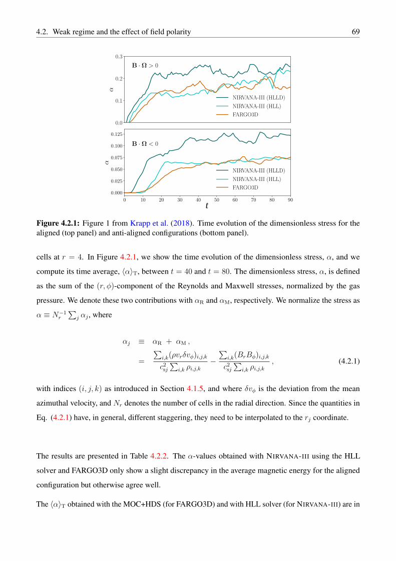
4.2. Weak regime and the effect of field polarity 69

t

Figure 4.2.1: Figure 1 from Krapp et al. (2018). Time evolution of the dimensionless stress for thealigned (top panel) and anti-aligned configurations (bottom panel).

cells at r = 4. In Figure 4.2.1, we show the time evolution of the dimensionless stress, α, and we

compute its time average, 〈α〉T, between t = 40 and t = 80. The dimensionless stress, α, is defined

as the sum of the (r, φ)-component of the Reynolds and Maxwell stresses, normalized by the gas

pressure. We denote these two contributions with αR and αM, respectively. We normalize the stress as

α ≡ N−1r

∑j αj , where

αj ≡ αR + αM ,

=

∑i,k(ρvrδvφ)i,j,k

c2sj

∑i,k ρi,j,k

−∑

i,k(BrBφ)i,j,k

c2sj

∑i,k ρi,j,k

, (4.2.1)

with indices (i, j, k) as introduced in Section 4.1.5, and where δvφ is the deviation from the mean

azimuthal velocity, and Nr denotes the number of cells in the radial direction. Since the quantities in

Eq. (4.2.1) have, in general, different staggering, they need to be interpolated to the rj coordinate.

The results are presented in Table 4.2.2. The α-values obtained with NIRVANA-III using the HLL

solver and FARGO3D only show a slight discrepancy in the average magnetic energy for the aligned

configuration but otherwise agree well.

The 〈α〉T obtained with the MOC+HDS (for FARGO3D) and with HLL solver (for NIRVANA-III) are in

70 4.2. Weak regime and the effect of field polarity

Table 4.2.2: Table 2 from Krapp et al. (2018). Measurements of the mean α-stress and magnetic energy

Hall-MHD 〈α〉T+ 〈α〉T− 〈EB〉T+ 〈EB〉T−F-3D (HDS) 0.17±0.02 0.066±0.004 0.32±0.03 0.12±0.01

N-III (HLL) 0.15±0.02 0.067±0.005 0.22±0.02 0.12±0.01

N-III (HDS) 0.23±0.02 0.12±0.01 0.30±0.04 0.17±0.02

Ideal-MHD 〈α〉 〈EB〉F-3D (HDS) 0.11±0.01 0.19±0.02

N-III (HDS) 0.16±0.01 0.25±0.03

Averages between t = 40− 80 for the different schemes. The magnetic energy, EB , is normalized to the initial pressure,i.e., EB ≡ B2/(2ρ0 c

2s ). Brackets 〈.〉T indicate time averages and the sign T± refers to the aligned (+) and anti-aligned

(−) configuration.

agreement with those reported by Béthune et al. (2016) but are larger than those reported by O’Keeffe

and Downes (2014), where 〈α〉T− ∼ 0.0092 and 〈α〉T+ ∼ 0.075 were obtained.

We moreover observe a difference between the time scales in which the MRI is found to saturate. We

obtain the saturation level after t = 20 for 〈α〉T+ and t = 30 for 〈α〉T−. In contrast, O’Keeffe and

Downes (2014) obtained that the stress saturates between 10 and 15 inner orbits. These differences

might be related to the use of a different sound speed. Also, because of the single-fluid approach, our

Hall diffusion coefficient only evolves with the magnetic field, whereas in the multifluid approach

presented by O’Keeffe and Downes (2014), this coefficient is also updated with the densities and

velocities of the charged species. Because of this, the models are likely not directly comparable.

Regarding the magnetic energy evolution, we recover a similar trend as seen by Béthune et al. (2016).

The magnetic energy has the same saturation timescale as the α-parameter, and remains stable around

a constant mean value between the inner orbits 30 and 90. This is another important difference with

respect to O’Keeffe and Downes (2014) where they found a secular growth as a function of time.

The 〈α〉T values obtained with NIRVANA-III using the HLLD solver are within 30% larger compared

with the ones from the other numerical schemes. We conjecture that this is simply a consequence of the

higher intrinsic accuracy of the HLLD scheme2, since the discrepancy persists for measurements of α

in ideal-MHD simulations. Using the same initial conditions as in Table 4.2.2, but setting LH = 0, we

found 〈α〉T+ = 0.16 with N-III, and 〈α〉T+ = 0.11 for F-3D.

2See Balsara and Meyer (2010) for a detailed study on the role of Riemann solvers and slope limiters in the context ofMRI in the ideal MHD limit.

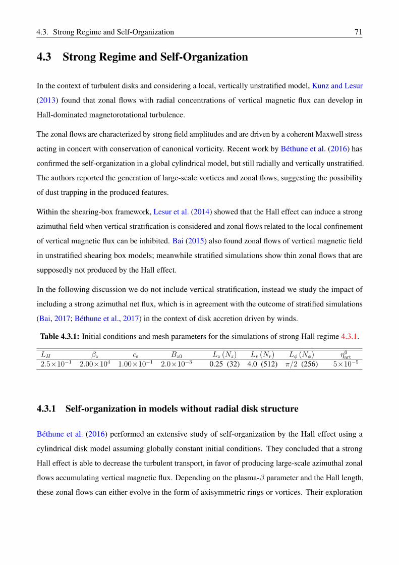
4.3. Strong Regime and Self-Organization 71

4.3 Strong Regime and Self-Organization

In the context of turbulent disks and considering a local, vertically unstratified model, Kunz and Lesur

(2013) found that zonal flows with radial concentrations of vertical magnetic flux can develop in

Hall-dominated magnetorotational turbulence.

The zonal flows are characterized by strong field amplitudes and are driven by a coherent Maxwell stress

acting in concert with conservation of canonical vorticity. Recent work by Béthune et al. (2016) has

confirmed the self-organization in a global cylindrical model, but still radially and vertically unstratified.

The authors reported the generation of large-scale vortices and zonal flows, suggesting the possibility

of dust trapping in the produced features.

Within the shearing-box framework, Lesur et al. (2014) showed that the Hall effect can induce a strong

azimuthal field when vertical stratification is considered and zonal flows related to the local confinement

of vertical magnetic flux can be inhibited. Bai (2015) also found zonal flows of vertical magnetic field

in unstratified shearing box models; meanwhile stratified simulations show thin zonal flows that are

supposedly not produced by the Hall effect.

In the following discussion we do not include vertical stratification, instead we study the impact of

including a strong azimuthal net flux, which is in agreement with the outcome of stratified simulations

(Bai, 2017; Béthune et al., 2017) in the context of disk accretion driven by winds.

Table 4.3.1: Initial conditions and mesh parameters for the simulations of strong Hall regime 4.3.1.

LH βz cs Bz0 Lz (Nz) Lr (Nr) Lφ (Nφ) η0art

2.5×10−1 2.00×104 1.00×10−1 2.0×10−3 0.25 (32) 4.0 (512) π/2 (256) 5×10−5

4.3.1 Self-organization in models without radial disk structure

Béthune et al. (2016) performed an extensive study of self-organization by the Hall effect using a

cylindrical disk model assuming globally constant initial conditions. They concluded that a strong

Hall effect is able to decrease the turbulent transport, in favor of producing large-scale azimuthal zonal

flows accumulating vertical magnetic flux. Depending on the plasma-β parameter and the Hall length,

these zonal flows can either evolve in the form of axisymmetric rings or vortices. Their exploration

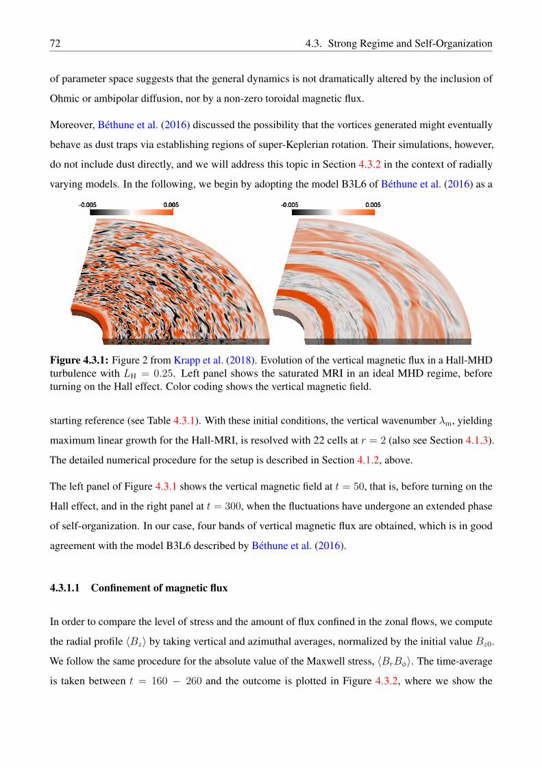
72 4.3. Strong Regime and Self-Organization

of parameter space suggests that the general dynamics is not dramatically altered by the inclusion of

Ohmic or ambipolar diffusion, nor by a non-zero toroidal magnetic flux.

Moreover, Béthune et al. (2016) discussed the possibility that the vortices generated might eventually

behave as dust traps via establishing regions of super-Keplerian rotation. Their simulations, however,

do not include dust directly, and we will address this topic in Section 4.3.2 in the context of radially

varying models. In the following, we begin by adopting the model B3L6 of Béthune et al. (2016) as a

Figure 4.3.1: Figure 2 from Krapp et al. (2018). Evolution of the vertical magnetic flux in a Hall-MHDturbulence with LH = 0.25. Left panel shows the saturated MRI in an ideal MHD regime, beforeturning on the Hall effect. Color coding shows the vertical magnetic field.

starting reference (see Table 4.3.1). With these initial conditions, the vertical wavenumber λm, yielding

maximum linear growth for the Hall-MRI, is resolved with 22 cells at r = 2 (also see Section 4.1.3).

The detailed numerical procedure for the setup is described in Section 4.1.2, above.

The left panel of Figure 4.3.1 shows the vertical magnetic field at t = 50, that is, before turning on the

Hall effect, and in the right panel at t = 300, when the fluctuations have undergone an extended phase

of self-organization. In our case, four bands of vertical magnetic flux are obtained, which is in good

agreement with the model B3L6 described by Béthune et al. (2016).

4.3.1.1 Confinement of magnetic flux

In order to compare the level of stress and the amount of flux confined in the zonal flows, we compute

the radial profile 〈Bz〉 by taking vertical and azimuthal averages, normalized by the initial value Bz0.

We follow the same procedure for the absolute value of the Maxwell stress, 〈BrBφ〉. The time-average

is taken between t = 160 − 260 and the outcome is plotted in Figure 4.3.2, where we show the

4.3. Strong Regime and Self-Organization 73

1.0 1.5 2.0 2.5 3.0 3.5 4.0 4.5 5.0r

−0.02

0.00

0.02

0.04

0.06

0.08

0.10 〈Ω/Ωk − 1〉|〈BrBφ〉|/|B0|2 × 10−1

〈Bz〉/|B0| × 10−2

Figure 4.3.2: Figure 3 from Krapp et al. (2018). Radial profiles of the vertical-azimuthal average ofthe vertical field, 〈Bz〉, the Maxwell stress, 〈BrBφ〉, and Ω/Ωk − 1. The solid curve correspond to thetime average between t = 160 and 260. Shaded areas indicate the standard deviation with respect to thetime average. The light-red shaded area indicates the sub-Keplerian velocity region.

confinement of the vertical zonal flows between regions of enhanced Maxwell stress.

This mechanism of confinement was first explained by Kunz and Lesur (2013) in the context of local

shearing box simulations and was studied in a cylindrical domain by Béthune et al. (2016). Using a

mean-field theory, they showed that the Hall effect introduces a component proportional to the turbulent

Maxwell stress in the evolution equation of the vertical magnetic field. This contribution of the Maxwell

stress might induce an extra dissipation (of either sign) added to the Ohmic diffusion. Thus it can favor

the accumulation of magnetic flux in regions of positive curvature of the mean Maxwell stress. After

the formation of the zonal flow, the turbulent field that lies in-between starts to flow into the regions

of confinement. This process generates a region of low stress and vanishing vertical flux between the

azimuthal bands. On the other hand, turbulent fluctuations may survive in regions located close to the

zonal flows, as is observed in Figure 4.3.2.

After around 300 orbits, the zonal flows remain quasi-stationary, and three separate zonal flows are

distinguishable, with a fourth one seeming to appear close the outer boundary at r ∼ 4. Figure 4.3.2

also shows that, on average, the Maxwell stress is larger near the radial buffer zones. Reflecting

boundary conditions adopted in the radial direction (enabling conservation of the magnetic flux to

machine precision) bring about the accumulation of magnetic flux close to the buffer zones, which

eventually may favor the concentration of Maxwell stress as well.

74 4.3. Strong Regime and Self-Organization

4.3.1.2 Effect on the azimuthal velocity

In addition to the averages of the Maxwell stress and the vertical field, we plot in Figure 4.3.2 the

vertically, azimuthally and time-averaged radial profile of Ω/ΩK − 1 indicating deviations of the

velocity field from Keplerian rotation (the light-red shaded region indicates sub-Keplerian rotation).

The emerging zonal flows introduce regions of super-Keplerian rotational velocity, which may act

locally to accumulate dust grains. We find in our runs that the velocity can reach a robust super-

Keplerian regime, constituting an efficient dust trap, that will prospectively produce an azimuthally

large-scale dust distribution. Note, however, that in the absence of a radial pressure gradient in the

background flow — as assumed in the models presented in this section — the gas initially rotates at the

Keplerian speed. In contrast, in a real disk, stellar irradiation heating and the density declines lead to a

radial pressure profile, which will, in general, decrease with radius. In that situation, the gas disk will

rotate on a slightly sub-Keplerian rotation profile, requiring a more vigorous effect to achieve regions

of super-Keplerian rotation.

4.3.2 Self-organization in models with radial disk structure

In this section we study the self-organization including a radially varying disk model. Furthermore, we

consider cases with different azimuthal net flux and include the dust as a pressureless fluid (see Section

3.2.3). The density and the sound speed are

ρg =Σ(r)√2πH(r)

, cs = cs0 r−pAU , (4.3.1)

with a surface density, Σ(r), and the hydrostatic scale height, H(r), defined as

Σ(r) = Σ0r−σAU and H(r) = cs/ΩK , (4.3.2)

respectively. We initialize the vertical and azimuthal magnetic field components as

Bz0 =

√2µ0ρgc2

s

βzand Bφ0 =

√2µ0ρgc2

s

βφ, (4.3.3)

respectively.

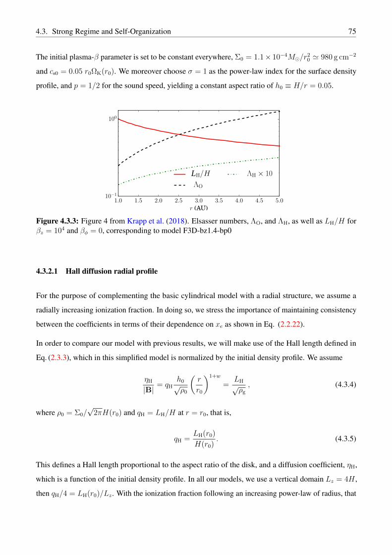
4.3. Strong Regime and Self-Organization 75

The initial plasma-β parameter is set to be constant everywhere, Σ0 = 1.1× 10−4M/r20 ' 980 g cm−2

and cs0 = 0.05 r0ΩK(r0). We moreover choose σ = 1 as the power-law index for the surface density

profile, and p = 1/2 for the sound speed, yielding a constant aspect ratio of h0 ≡ H/r = 0.05.

L

Figure 4.3.3: Figure 4 from Krapp et al. (2018). Elsasser numbers, ΛO, and ΛH, as well as LH/H forβz = 104 and βφ = 0, corresponding to model F3D-bz1.4-bp0

4.3.2.1 Hall diffusion radial profile

For the purpose of complementing the basic cylindrical model with a radial structure, we assume a

radially increasing ionization fraction. In doing so, we stress the importance of maintaining consistency

between the coefficients in terms of their dependence on xe as shown in Eq. (2.2.22).

In order to compare our model with previous results, we will make use of the Hall length defined in

Eq. (2.3.3), which in this simplified model is normalized by the initial density profile. We assume

ηH

|B| = qHh0√ρ0

(r

r0

)1+w

=LH√ρg

, (4.3.4)

where ρ0 = Σ0/√

2πH(r0) and qH = LH/H at r = r0, that is,

qH =LH(r0)

H(r0). (4.3.5)

This defines a Hall length proportional to the aspect ratio of the disk, and a diffusion coefficient, ηH,

which is a function of the initial density profile. In all our models, we use a vertical domain Lz = 4H ,

then qH/4 = LH(r0)/Lz. With the ionization fraction following an increasing power-law of radius, that

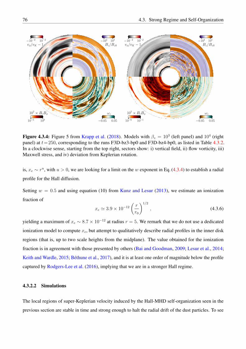
76 4.3. Strong Regime and Self-Organization

vφ/vK − 1 Bz/Bz0

107 × BrBφ ωz

−101 101−10−2 10−2

10−5 100 −0.05 0.05

vφ/vK − 1 Bz/Bz0

107 × BrBφ ωz

−101 101−10−2 10−2

10−6 10−1 −0.05 0.05

Figure 4.3.4: Figure 5 from Krapp et al. (2018). Models with βz = 103 (left panel) and 104 (rightpanel) at t=250, corresponding to the runs F3D-bz3-bp0 and F3D-bz4-bp0, as listed in Table 4.3.2.In a clockwise sense, starting from the top right, sectors show: i) vertical field, ii) flow vorticity, iii)Maxwell stress, and iv) deviation from Keplerian rotation.

is, xe ∼ ru, with u > 0, we are looking for a limit on the w exponent in Eq. (4.3.4) to establish a radial

profile for the Hall diffusion.

Setting w = 0.5 and using equation (10) from Kunz and Lesur (2013), we estimate an ionization

fraction of

xe ' 3.9× 10−12

(r

r0

)1/2

, (4.3.6)

yielding a maximum of xe ∼ 8.7× 10−12 at radius r = 5. We remark that we do not use a dedicated

ionization model to compute xe, but attempt to qualitatively describe radial profiles in the inner disk

regions (that is, up to two scale heights from the midplane). The value obtained for the ionization

fraction is in agreement with those presented by others (Bai and Goodman, 2009; Lesur et al., 2014;

Keith and Wardle, 2015; Béthune et al., 2017), and it is at least one order of magnitude below the profile

captured by Rodgers-Lee et al. (2016), implying that we are in a stronger Hall regime.

4.3.2.2 Simulations

The local regions of super-Keplerian velocity induced by the Hall-MHD self-organization seen in the

previous section are stable in time and strong enough to halt the radial drift of the dust particles. To see

4.3. Strong Regime and Self-Organization 77

whether this trend holds for more realistic disk models, we study the conditions for dust trapping in a

protoplanetary disk extended between 1− 5 AU, using the disk model defined in Section 4.3.2, focusing

on results obtained with FARGO3D. The standard computational domain is z ∈ [0, 4h0], r ∈ [1, 5], and

φ ∈ [0, π/2], resolved with 32× 256× 512 grid cells, respectively. We use a logarithmic spacing in the

radial direction to maintain a constant radial resolution per gas pressure scale-height.

Vertical and azimuthal magnetic field components are defined via constant βz and βφ, respectively. The

aspect ratio is set to h0 = 0.05, and the initial angular velocity of the gas is Keplerian3. We add a white

noise initial perturbation in the vertical and radial components of the velocity field in order to seed and

grow the MRI in the ideal MHD limit. After t = 40 orbital periods, we switch on the Hall effect and

Ohmic diffusion, and we further evolve the model until t = 300.

The Hall diffusion coefficient, as introduced in Section 2.2 — see Eqs. (4.3.4) and (4.3.5) — is given by

ηH(r) = qHh0√ρ0

(r

r0

)1+w

|B| , (4.3.7)

with w = 0.5. We adopt an initial qH = 1 at r = r0, but we also run models with qH = 2, and qH = 4.

The Ohmic diffusion profile is given by ηO(r) = η0 r−1/2, and we set η0 = 2× 10−6, which gives an

initial ΛO∼< 1 throughout the radial domain. In Figure 4.3.3, we show the initial Elsasser numbers

computed with βz = 104 and βφ =∞.

All the runs are listed in 4.3.2 with a nomenclature as follows:

FARGO3D− βz = 5× 103 − βφ =∞− qH = 2− azimuthal domain = 2π → F3D-bz5.3-bp0-2-2d

FARGO3D− βz = 5× 103 − βφ =∞− qH = 1− azimuthal domain = π/2→ F3D-bz5.3-bp0

4.3.2.3 Self-organization for different vertical fields

We first discuss the runs with a fixed βz and varying qH, and then turn to results using three different

initial βz, while keeping qH fixed.

3The flow adjusts to the sub-Keplerian equilibrium during the first orbit.

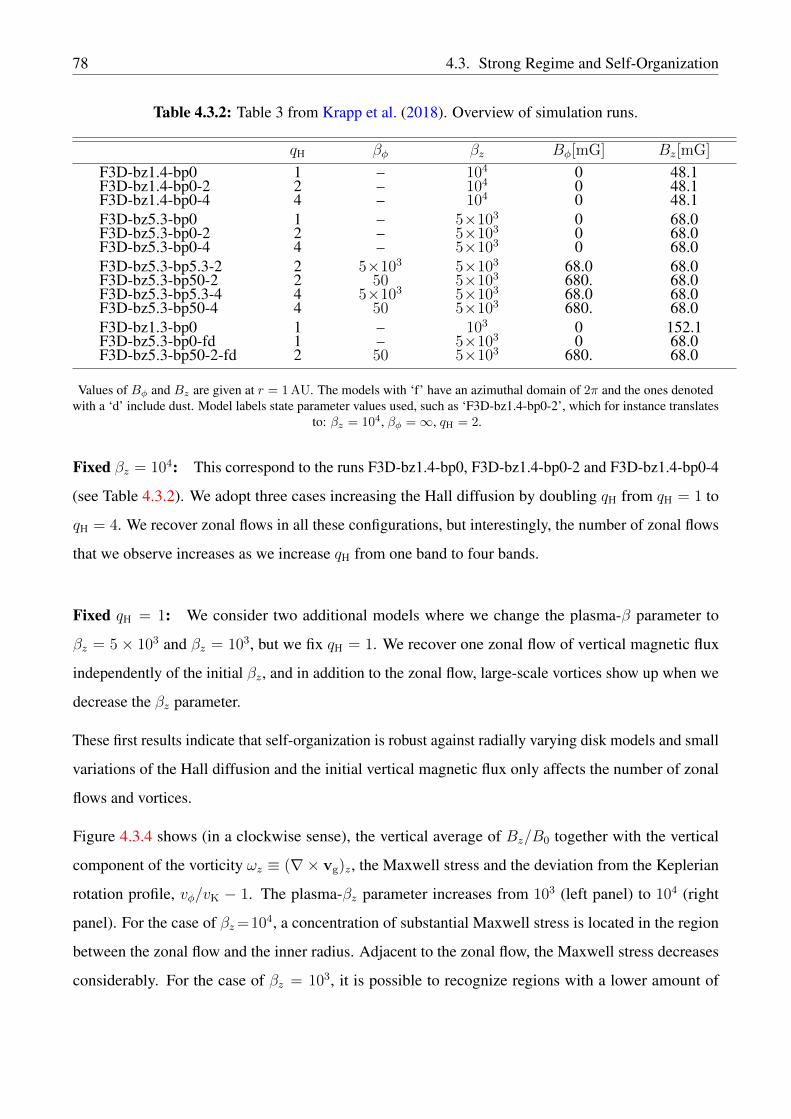
78 4.3. Strong Regime and Self-Organization

Table 4.3.2: Table 3 from Krapp et al. (2018). Overview of simulation runs.

qH βφ βz Bφ[mG] Bz[mG]

F3D-bz1.4-bp0 1 – 104 0 48.1F3D-bz1.4-bp0-2 2 – 104 0 48.1F3D-bz1.4-bp0-4 4 – 104 0 48.1F3D-bz5.3-bp0 1 – 5×103 0 68.0F3D-bz5.3-bp0-2 2 – 5×103 0 68.0F3D-bz5.3-bp0-4 4 – 5×103 0 68.0F3D-bz5.3-bp5.3-2 2 5×103 5×103 68.0 68.0F3D-bz5.3-bp50-2 2 50 5×103 680. 68.0F3D-bz5.3-bp5.3-4 4 5×103 5×103 68.0 68.0F3D-bz5.3-bp50-4 4 50 5×103 680. 68.0F3D-bz1.3-bp0 1 – 103 0 152.1F3D-bz5.3-bp0-fd 1 – 5×103 0 68.0F3D-bz5.3-bp50-2-fd 2 50 5×103 680. 68.0

Values of Bφ and Bz are given at r = 1 AU. The models with ‘f’ have an azimuthal domain of 2π and the ones denotedwith a ‘d’ include dust. Model labels state parameter values used, such as ‘F3D-bz1.4-bp0-2’, which for instance translates

to: βz = 104, βφ =∞, qH = 2.

Fixed βz = 104: This correspond to the runs F3D-bz1.4-bp0, F3D-bz1.4-bp0-2 and F3D-bz1.4-bp0-4

(see Table 4.3.2). We adopt three cases increasing the Hall diffusion by doubling qH from qH = 1 to

qH = 4. We recover zonal flows in all these configurations, but interestingly, the number of zonal flows

that we observe increases as we increase qH from one band to four bands.

Fixed qH = 1: We consider two additional models where we change the plasma-β parameter to

βz = 5× 103 and βz = 103, but we fix qH = 1. We recover one zonal flow of vertical magnetic flux

independently of the initial βz, and in addition to the zonal flow, large-scale vortices show up when we

decrease the βz parameter.

These first results indicate that self-organization is robust against radially varying disk models and small

variations of the Hall diffusion and the initial vertical magnetic flux only affects the number of zonal

flows and vortices.

Figure 4.3.4 shows (in a clockwise sense), the vertical average of Bz/B0 together with the vertical

component of the vorticity ωz ≡ (∇× vg)z, the Maxwell stress and the deviation from the Keplerian

rotation profile, vφ/vK − 1. The plasma-βz parameter increases from 103 (left panel) to 104 (right

panel). For the case of βz=104, a concentration of substantial Maxwell stress is located in the region

between the zonal flow and the inner radius. Adjacent to the zonal flow, the Maxwell stress decreases

considerably. For the case of βz = 103, it is possible to recognize regions with a lower amount of

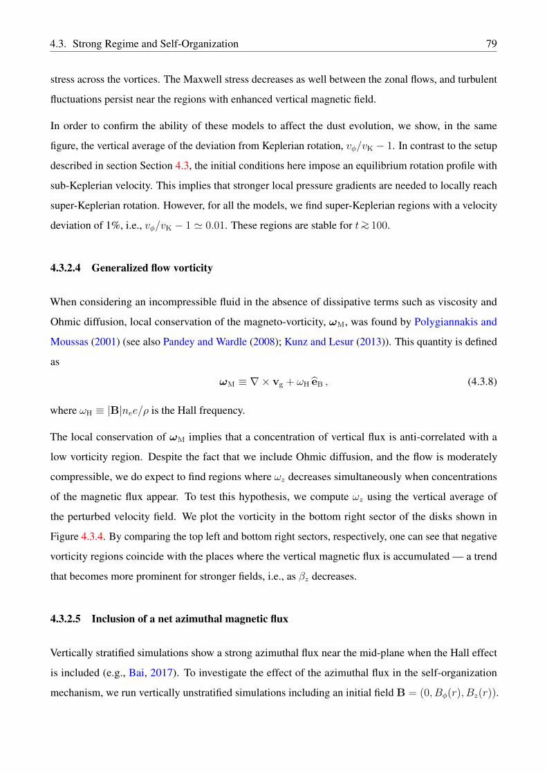
4.3. Strong Regime and Self-Organization 79

stress across the vortices. The Maxwell stress decreases as well between the zonal flows, and turbulent

fluctuations persist near the regions with enhanced vertical magnetic field.

In order to confirm the ability of these models to affect the dust evolution, we show, in the same

figure, the vertical average of the deviation from Keplerian rotation, vφ/vK − 1. In contrast to the setup

described in section Section 4.3, the initial conditions here impose an equilibrium rotation profile with

sub-Keplerian velocity. This implies that stronger local pressure gradients are needed to locally reach

super-Keplerian rotation. However, for all the models, we find super-Keplerian regions with a velocity

deviation of 1%, i.e., vφ/vK − 1 ' 0.01. These regions are stable for t∼> 100.

4.3.2.4 Generalized flow vorticity

When considering an incompressible fluid in the absence of dissipative terms such as viscosity and

Ohmic diffusion, local conservation of the magneto-vorticity, ωM, was found by Polygiannakis and

Moussas (2001) (see also Pandey and Wardle (2008); Kunz and Lesur (2013)). This quantity is defined

as

ωM ≡ ∇× vg + ωH eB , (4.3.8)

where ωH ≡ |B|nee/ρ is the Hall frequency.

The local conservation of ωM implies that a concentration of vertical flux is anti-correlated with a

low vorticity region. Despite the fact that we include Ohmic diffusion, and the flow is moderately

compressible, we do expect to find regions where ωz decreases simultaneously when concentrations

of the magnetic flux appear. To test this hypothesis, we compute ωz using the vertical average of

the perturbed velocity field. We plot the vorticity in the bottom right sector of the disks shown in

Figure 4.3.4. By comparing the top left and bottom right sectors, respectively, one can see that negative

vorticity regions coincide with the places where the vertical magnetic flux is accumulated — a trend

that becomes more prominent for stronger fields, i.e., as βz decreases.

4.3.2.5 Inclusion of a net azimuthal magnetic flux

Vertically stratified simulations show a strong azimuthal flux near the mid-plane when the Hall effect

is included (e.g., Bai, 2017). To investigate the effect of the azimuthal flux in the self-organization

mechanism, we run vertically unstratified simulations including an initial field B = (0, Bφ(r), Bz(r)).

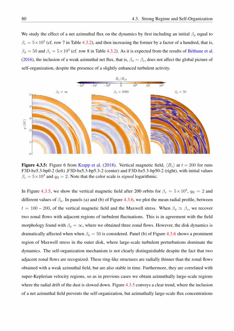
80 4.3. Strong Regime and Self-Organization

We study the effect of a net azimuthal flux on the dynamics by first including an initial βφ equal to

βz = 5×103 (cf. row 7 in Table 4.3.2), and then increasing the former by a factor of a hundred, that is,

βφ = 50 and βz = 5×103 (cf. row 8 in Table 4.3.2). As it is expected from the results of Béthune et al.

(2016), the inclusion of a weak azimuthal net flux, that is, βφ ∼ βz, does not affect the global picture of

self-organization, despite the presence of a slightly enhanced turbulent activity.

0

1

2

3

4

5

y(A

U)

βφ =∞ βφ = 5000

−102 −101 −100 0 100 101 102

Bz/Bz0

βφ = 50

Figure 4.3.5: Figure 6 from Krapp et al. (2018). Vertical magnetic field, 〈Bz〉 at t = 200 for runsF3D-bz5.3-bp0-2 (left) ,F3D-bz5.3-bp5.3-2 (center) and F3D-bz5.3-bp50-2 (right), with initial valuesβz = 5×103 and qH = 2. Note that the color scale is signed logarithmic.

In Figure 4.3.5, we show the vertical magnetic field after 200 orbits for βz = 5×103, qH = 2 and

different values of βφ. In panels (a) and (b) of Figure 4.3.6, we plot the mean radial profile, between

t = 100 – 200, of the vertical magnetic field and the Maxwell stress. When βφ ' βz, we recover

two zonal flows with adjacent regions of turbulent fluctuations. This is in agreement with the field

morphology found with βφ =∞, where we obtained three zonal flows. However, the disk dynamics is

dramatically affected when when βφ = 50 is considered. Panel (b) of Figure 4.3.6 shows a prominent

region of Maxwell stress in the outer disk, where large-scale turbulent perturbations dominate the

dynamics. The self-organization mechanism is not clearly distinguishable despite the fact that two

adjacent zonal flows are recognized. These ring-like structures are radially thinner than the zonal flows

obtained with a weak azimuthal field, but are also stable in time. Furthermore, they are correlated with

super-Keplerian velocity regions, so as in previous cases we obtain azimuthally large-scale regions

where the radial drift of the dust is slowed down. Figure 4.3.5 conveys a clear trend, where the inclusion

of a net azimuthal field prevents the self-organization, but azimuthally large-scale flux concentrations

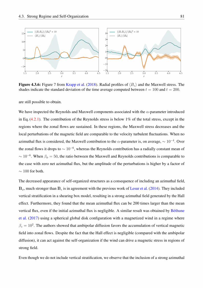
4.3. Strong Regime and Self-Organization 81

1.5 2.0 2.5 3.0 3.5 4.0 4.5r

−5

0

5

10

15|〈BrBφ〉|/|B0|2 × 10

〈Bz〉/|B0|

1.5 2.0 2.5 3.0 3.5 4.0 4.5r

−2

−1

0

1

2

3

4|〈BrBφ〉|/|B0|2 × 10

〈Bz〉/|B0|

Figure 4.3.6: Figure 7 from Krapp et al. (2018). Radial profiles of 〈Bz〉 and the Maxwell stress. Theshades indicate the standard deviation of the time average computed between t = 100 and t = 200.

are still possible to obtain.

We have inspected the Reynolds and Maxwell components associated with the α-parameter introduced

in Eq. (4.2.1). The contribution of the Reynolds stress is below 1% of the total stress, except in the

regions where the zonal flows are sustained. In these regions, the Maxwell stress decreases and the

local perturbations of the magnetic field are comparable to the velocity turbulent fluctuations. When no

azimuthal flux is considered, the Maxwell contribution to the α-parameter is, on average, ∼ 10−4. Over

the zonal flows it drops to ∼ 10−6, whereas the Reynolds contribution has a radially constant mean of

∼ 10−6. When βφ = 50, the ratio between the Maxwell and Reynolds contributions is comparable to

the case with zero net azimuthal flux, but the amplitude of the perturbations is higher by a factor of

∼ 100 for both.

The decreased appearance of self-organized structures as a consequence of including an azimuthal field,

Bφ, much stronger than Bz is in agreement with the previous work of Lesur et al. (2014). They included

vertical stratification in a shearing box model, resulting in a strong azimuthal field generated by the Hall

effect. Furthermore, they found that the mean azimuthal flux can be 200 times larger than the mean

vertical flux, even if the initial azimuthal flux is negligible. A similar result was obtained by Béthune

et al. (2017) using a spherical global disk configuration with a magnetized wind in a regime where

βz = 102. The authors showed that ambipolar diffusion favors the accumulation of vertical magnetic

field into zonal flows. Despite the fact that the Hall effect is negligible (compared with the ambipolar

diffusion), it can act against the self-organization if the wind can drive a magnetic stress in regions of

strong field.

Even though we do not include vertical stratification, we observe that the inclusion of a strong azimuthal

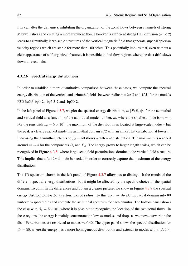
82 4.3. Strong Regime and Self-Organization

flux can alter the dynamics, inhibiting the organization of the zonal flows between channels of strong

Maxwell stress and creating a more turbulent flow. However, a sufficient strong Hall diffusion (qH∼> 2)

leads to azimuthally large-scale structures of the vertical magnetic field that generate super-Keplerian

velocity regions which are stable for more than 100 orbits. This potentially implies that, even without a

clear appearance of self-organized features, it is possible to find flow regions where the dust drift slows

down or even halts.

4.3.2.6 Spectral energy distributions

In order to establish a more quantitative comparison between these cases, we compute the spectral

energy distribution of the vertical and azimuthal fields between radius r=2AU and 4AU for the models

F3D-bz5.3-bp0-2, -bp5.3-2 and -bp50-2.

In the left panel of Figure 4.3.7, we plot the spectral energy distribution, m |F(Bi)|2, for the azimuthal

and vertical field as a function of the azimuthal mode number, m, where the smallest mode is m = 4.

For the runs with βφ = 5× 103, the maximum of the distribution is located at large-scale modes – but

the peak is clearly reached inside the azimuthal domain π/2 with an almost flat distribution at lower m.

Increasing the azimuthal net-flux to βφ = 50 shows a different distribution. The maximum is reached

around m ∼ 4 for the components Bz and Bφ. The energy grows to larger length scales, which can be

recognized in Figure 4.3.5, where large-scale field perturbations dominate the vertical field structure.

This implies that a full 2π domain is needed in order to correctly capture the maximum of the energy

distribution.

The 1D spectrum shown in the left panel of Figure 4.3.7 allows us to distinguish the trends of the

different spectral energy distributions, but it might be affected by the specific choice of the spatial

domain. To confirm the differences and obtain a clearer picture, we show in Figure 4.3.7 the spectral

energy distribution for Bz as a function of radius. To this end, we divide the radial domain into 80

uniformly-spaced bins and compute the azimuthal spectrum for each annulus. The bottom panel shows

the case with βφ = 5×103, where it is possible to recognize the location of the two zonal flows. In

these regions, the energy is mainly concentrated in low-m modes, and drops as we move outward in the

disk. Perturbations are restricted to modes m∼< 40. The upper panel shows the spectral distribution for

βφ = 50, where the energy has a more homogeneous distribution and extends to modes with m∼> 100.

4.3. Strong Regime and Self-Organization 83

101 102

m

10−13

10−12

10−11

10−10

10−9

10−8

10−7

10−6

m|F

(Bi)|2

βφ =∞βφ = 5000

βφ = 50

1.2 1.6 2.0 2.4 2.8 3.2 3.6 4.0 4.4 4.8

r

20

40

60

80

100

120

m

−13 −12 −11 −10 −9 −8

log10 |F(Bz)|2 - βφ = 50

1.2 1.6 2.0 2.4 2.8 3.2 3.6 4.0 4.4 4.8

r

20

40

60

80

100

120

m

−13 −12 −11 −10 −9 −8

log10 |F(Bz)|2 - βφ = 5000

Figure 4.3.7: Figures 8 and 9 from Krapp et al. (2018). Spectral energy distribution, m |F(Bs)|2, forBz (solid lines) and Bφ (dotted lines) for weak and strong azimuthal net flux (averaged between t = 190and t = 210). Spectral energy distribution |F(Bz)|2, for 80 radial uniform bins, averaged betweent = 190, 210. Top: run F3D-bz3.5-bp50 with βφ = 50. Bottom: run -bp5.3 with βφ = 5000.

4.3.2.7 Dynamics of Embedded Dust Grains

−101 101

Bz/Bz0

0.2 1.8

ρd/ρd0 St=1

0.6 1.4

ρd/ρd0 St=0.1

0.6 1.4

ρd/ρd0 St=0.01

Figure 4.3.8: Figure 10 from Krapp et al. (2018). Vertical average for Bz/Bz0 (leftmost panel) anddust density contrast ρd/ρd0 (remaining three panels) for t = 250. The dust density contrast is shown inorder of decreasing Stokes number (referred as St instead of Ts) of 1, 0.1, and 0.01, respectively. Theupper row corresponds to model F3D-bz5.3-bp0-fd, without an azimuthal field, and the bottom rowcorresponds to the model F3D-bz5.3-bp50-fd, with a dominant azimuthal field.

In view of the azimuthally large-scale morphology of the flux concentrations, and accommodating for

the fact that the spectral energy distribution is dominated by low azimuthal wavenumbers, we now

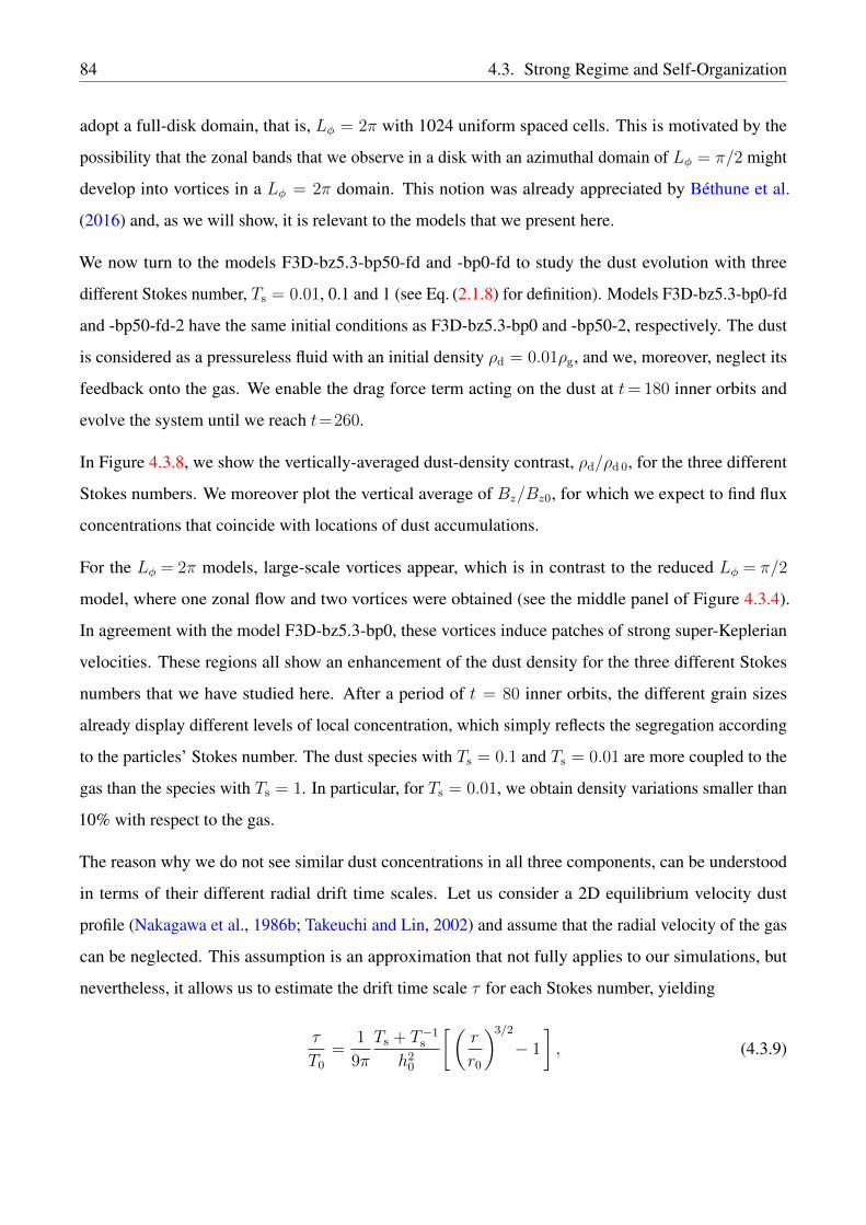
84 4.3. Strong Regime and Self-Organization

adopt a full-disk domain, that is, Lφ = 2π with 1024 uniform spaced cells. This is motivated by the

possibility that the zonal bands that we observe in a disk with an azimuthal domain of Lφ = π/2 might

develop into vortices in a Lφ = 2π domain. This notion was already appreciated by Béthune et al.

(2016) and, as we will show, it is relevant to the models that we present here.

We now turn to the models F3D-bz5.3-bp50-fd and -bp0-fd to study the dust evolution with three

different Stokes number, Ts = 0.01, 0.1 and 1 (see Eq. (2.1.8) for definition). Models F3D-bz5.3-bp0-fd

and -bp50-fd-2 have the same initial conditions as F3D-bz5.3-bp0 and -bp50-2, respectively. The dust

is considered as a pressureless fluid with an initial density ρd = 0.01ρg, and we, moreover, neglect its

feedback onto the gas. We enable the drag force term acting on the dust at t= 180 inner orbits and

evolve the system until we reach t=260.

In Figure 4.3.8, we show the vertically-averaged dust-density contrast, ρd/ρd 0, for the three different

Stokes numbers. We moreover plot the vertical average of Bz/Bz0, for which we expect to find flux

concentrations that coincide with locations of dust accumulations.

For the Lφ = 2π models, large-scale vortices appear, which is in contrast to the reduced Lφ = π/2

model, where one zonal flow and two vortices were obtained (see the middle panel of Figure 4.3.4).

In agreement with the model F3D-bz5.3-bp0, these vortices induce patches of strong super-Keplerian

velocities. These regions all show an enhancement of the dust density for the three different Stokes

numbers that we have studied here. After a period of t = 80 inner orbits, the different grain sizes

already display different levels of local concentration, which simply reflects the segregation according

to the particles’ Stokes number. The dust species with Ts = 0.1 and Ts = 0.01 are more coupled to the

gas than the species with Ts = 1. In particular, for Ts = 0.01, we obtain density variations smaller than

10% with respect to the gas.

The reason why we do not see similar dust concentrations in all three components, can be understood

in terms of their different radial drift time scales. Let us consider a 2D equilibrium velocity dust

profile (Nakagawa et al., 1986b; Takeuchi and Lin, 2002) and assume that the radial velocity of the gas

can be neglected. This assumption is an approximation that not fully applies to our simulations, but

nevertheless, it allows us to estimate the drift time scale τ for each Stokes number, yielding

τ

T0

=1

9π

Ts + T−1s

h20

[(r

r0

)3/2

− 1

], (4.3.9)

4.3. Strong Regime and Self-Organization 85

0

5

10

ρd/ρ

d0 St=1

1

2

3

ρd/ρ

d0 St=0.1

0.9

1.0

1.1

ρd/ρ

d0 St=0.01

−0.5

0.0

102×

(Ω/Ω

k−

1)

2.0 2.5 3.0 3.5 4.0r

0

5

Bz/B

z0

0.0

2.5

5.0

7.5

ρd/ρ

d0 St=1

1

2

ρd/ρ

d0 St=0.1

0.75

1.00

1.25

ρd/ρ

d0 St=0.01

−1.0

−0.5

0.0

102×

(Ω/Ω

k−

1)

2.0 2.5 3.0 3.5 4.0r

0

20

Bz/B

z0

Figure 4.3.9: Figure 10 from Krapp et al. (2018). Mean radial profiles (averaged between t = 190−260)for models F3D-bz5.3-bp0-fd, with zero azimuthal flux (left panel), and F3D-bz5.3-bp50-fd, with astrong azimuthal flux (right panel). Dashed lines indicate the (sub-Keplerian) equilibrium velocityprofile.

where T0 = 2π/Ω0. If we consider a trap located at r = 3, the drift time scale is τ/T0 ' 118 inner

orbits for unity Stokes number – meanwhile, for Ts = 0.01, it is around τ/T0 ' 6×103, so we need to

integrate for 6000 orbits for Ts = 0.01 in order to cover the same fraction of the drift timescale as that

of the species with Ts = 1.

Figure 4.3.9 shows azimuthally averaged radial profiles of the dust-density ratios ρd/ρd 0, along with the

deviation, Ω/ΩK − 1, from Keplerian rotation, and the vertical magnetic field enhancement, Bz/Bz0.

Despite not being axisymmetric, the vortical structures are sufficiently large in their azimuthal extent

that averaging the velocity deviation in the toroidal direction will enhance regions were the dust

accumulations are stable in time. Taking azimuthal averages moreover brings out regions where the

average velocity field becomes almost super-Keplerian over significant intervals of time – even though

the super-Keplerian rotation of the vortices does get washed-out by taking the mean. This allows us

to identify the radial locations of strong magnetic flux concentrations and recognize that these are the

regions of dust enhancement. For Stokes number Ts = 1, in some locations, the density contrast reaches

86 4.4. Summary and Conclusions

a peak of ρd/ρd 0 ' 10. For longer times, it might reach even higher values, and the feedback onto the

gas can no longer be neglected.

In agreement with the discussion in section Section 4.3.2.5, the inclusion of a strong azimuthal field

induces large-scale concentrations of the vertical magnetic field, which in this particular case can be

axisymmetric. These regions are generally stable in time and induce super-Keplerian flows. The profiles

shown in the right panel of Figure 4.3.9 highlight the coincidence of these locations with the dust

enhancements.

4.4 Summary and Conclusions

Weak Hall regime: The inclusion of the Hall effect with different magnetic field polarity significantly

affects the non-linear evolution of the turbulent flow. In our configuration, the case with B parallel

to Ω shows an average α-value that is larger with respect to the anti-parallel case. Furthermore, our

findings agree with the previous results from Béthune et al. (2016) in the simulations performed with

both NIRVANA-III (with HLL) and FARGO3D, which validates the numerical implementation of the

Hall effect in both codes.

Self-organization: Comparison with previous work. Adopting a different numerical approach, we

have reproduced a similar setup for a disk with no initial radial structure, as is described in Béthune et al.

(2016) (see B3L6). We found four regions where vertical magnetic flux is confined, which is in excellent

agreement with the mentioned previous work. This result validates the numerical implementation in

FARGO3D in a strong Hall regime with the inclusion of artificial Ohmic resistivity.

Self-organization with azimuthal net flux. We simulated disks models with different azimuthal

and vertical net flux. For a plasma-β parameter in the range βz = 104 − 103, our results show minor

differences between cases with zero azimuthal net flux and cases where the azimuthal flux is comparable

to the vertical flux. When the initial model has a strong azimuthal net flux, i.e., βφ ' 10−2×βz, it is

still possible to obtain azimuthally large-scale concentrations of vertical magnetic flux. However, the

picture of field confinement between regions of enhanced Maxwell stress is no longer identified in

these simulations. Besides, when the azimuthal component of the magnetic field strongly dominates the

4.4. Summary and Conclusions 87

dynamics, the self-organized zonal flows are harder to recover, which is in agreement with previous

results from Lesur et al. (2014) and Béthune et al. (2017).

Self-organization and disk azimuthal domain: Simulations, with azimuthal domain reduced to

Lφ = π/2, show axisymmetric zonal flows and vortices; however, we are only able to recognize large-

scale vortical features if the domain is Lφ=2π. We studied the spectral energy distribution considering

different azimuthal domains and found that the maximum of energy increases as we move towards

shorter azimuthal wavenumber, m ' 4. We furthermore compared the spectral energy distributions of

the models with different azimuthal net flux but in an azimuthal domain of π/2. When βφ = 5×103,

the distribution shows a maximum followed by a flat profile at the lower azimuthal modes. Increasing

βφ leads to a spectrum that has a peak at intermediate azimuthal wavenumbers.

Self-organization and magneto-vorticity: Our findings confirm that the zonal flows (and vortices)

are confined between regions of strong Maxwell stress — in agreement with the mechanism described

by Kunz and Lesur (2013). Because of the low flow compressibility and the inclusion of small Ohmic

dissipation, the vortices and zonal flows are anti-correlated with low vorticity regions, which is expected

when the magneto-vorticity is locally conserved.

Self-organization and dust evolution: By including the evolution of pressureless dust fluids in the

ensuing Hall-MHD turbulence, we demonstrate that quasi-axisymmetric dust enhancements can be

obtained for the range of Stokes numbers explored – even in the absence of prominent flow features,

such as the result of Hall-effect induced self-organization. There appears to be a difference in character

regarding the precise nature of the ensuing dust traps, however. In models without azimuthal net flux,

dust enhancements are typically located at the position of vortices themselves, which agrees well with

the notion of vortices being able to trap dust (Klahr and Henning, 1997). In contrast to this, in models

with significant azimuthal magnetic flux (βφ ' 50), the dust accumulations appear to coincide with

local concentrations of the vertical magnetic flux.

Dust evolution for different Stokes numbers: For particles with Stokes number Ts =1, peaks in the

dust concentration with ρd/ρd0 ' 20 are reached during the integration time of a few hundred inner

orbits that we have adopted here, implying that the feedback onto the gas might have to be considered

88 4.4. Summary and Conclusions

when pursuing longer integration times. The drift time scale of the Ts = 0.1 and Ts = 0.01 particles

can be estimated to be between one and two orders of magnitude higher than that for Ts = 1. As a

result, lower dust enhancement factors were obtained for these two dust species, which we, at least

partially, attribute to the insufficient evolution time covered by our current simulations.

5Multispecies Streaming Instability

The aerodynamic coupling between solids and gas in a differentially rotating disk leads to the so-called

streaming instability (Youdin and Goodman, 2005). Depending on the dust-to-gas density ratio and

the collision frequency, the instability can grow on relatively short time scales, comparable to a few

tenths of orbits of the PPD. Higher dust concentrations and larger particle-sizes show the fastest growth

(Youdin and Goodman, 2005; Youdin and Johansen, 2007). The primary outcome of the non-linear

evolution is the formation of clumps or filaments where conditions are favorable for gravitational

collapse (Johansen and Youdin, 2007; Simon et al., 2016). Thus, this instability is thought to play a

central role in the early stages of planet formation by enabling the efficient bypass of several barriers

hindering the formation of planetesimals.

In this chapter, we offer an extended discussion about the linear and the non-linear phase of the

streaming instability. We adopt a different derivation than the one presented by Youdin and Goodman

(2005), by considering a compressible regime where the background drift induced by the gas pressure

gradient is obtained, defining an external force. Besides, our equations are not at the center-of-mass

reference frame, and we consider an arbitrary number of dust species.

In Section 5.1.1, we present the steady-state analytical solutions for the drift velocity of multiple dust

species, generalizing the obtained by Nakagawa et al. (1986a). We derive analytical closed expressions

for the background velocities, an important difference concerning the solutions found by Bai and Stone

(2010a). In Section 5.1.2 we present the linearized equations and in Section 5.1.3 we present numerical

results that validate both our analytical framework and the numerical approach discussed in Chapter

3. In Section 5.2, we study the linear phase of the streaming instability and show how the inclusion

of multiple species impose secular timescales for the linear growth. Finally, in Section 5.3, we show

89

90 5.1. Streaming instability

the non-linear evolution of the two-fluid streaming instability, successfully recovering the dynamics

previously obtained by other authors using Lagrangian particles. Most of the following discussions,

tables and figures, were published in Benítez-Llambay et al. (2019) and Krapp et al. (2019).

5.1 Streaming instability

To obtain the linear growth rate of the streaming-instability, we solve the 2.5D linearized axisymmetric

shearing-box equations for gas and one dust species. The fluid equations linearization is usually done

around the steady-state drift solution obtained by Nakagawa et al. (1986a). However, in order to study

the instability for an arbitrary number of dust species, generalized background solutions are needed.

These are similar to the approximated solutions obtained for the global disk (see Section 3.4.1), but

in this case are analytical. Furthermore, the solution is exact because velocities are not first-order

expanded as in the global case. We derive and write them explicitly in Section 5.1.1.

When the background density is assumed constant in the shearing-box approximation, a self-consistent

sub-Keplerian background velocity for the gas cannot be obtained. However, to study the instability in

this formalism, we add a constant external force mimicking the effect of a constant pressure gradient

within the box (see e.g. Bai and Stone, 2010b).

The equations leading to the streaming instability, when N dust species are considered, are

∂tρg +∇ · (ρgvg) = 0 , (5.1.1)

∂tρj +∇ · (ρjvj) = 0 , (5.1.2)

∂tvg + vg · ∇vg =− ∇Pρg

+ χ0Ω0ex + 2qΩ20xex

− 2Ω0 × vg − Ω0

N∑

k=1

εk∆k

Tsk

, (5.1.3)

∂tvj + vj · ∇vj =2qΩ20xex − 2Ω0 × vj + Ω0

∆j

Tsj

, (5.1.4)

for j = 1, . . . , N , with q the shear parameter. The term χ0Ω0 is the constant radial acceleration that

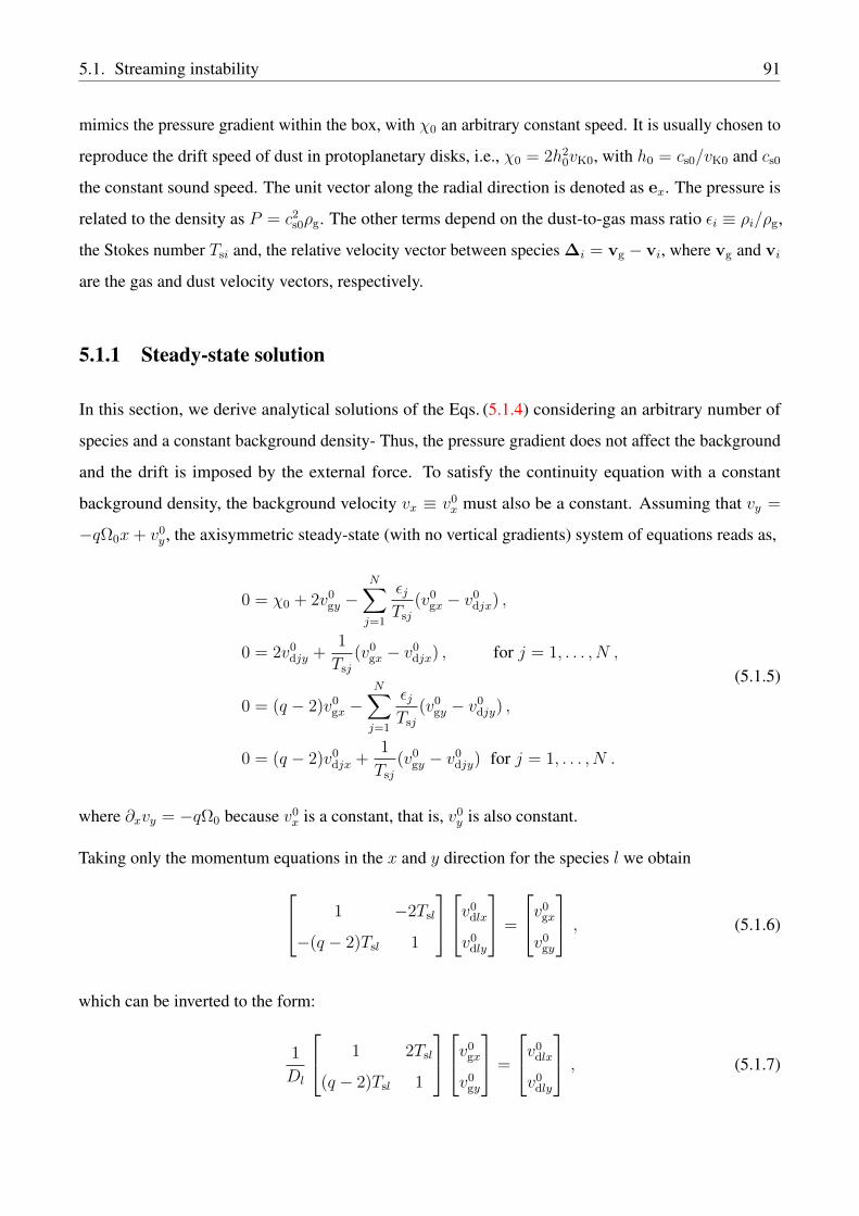
5.1. Streaming instability 91

mimics the pressure gradient within the box, with χ0 an arbitrary constant speed. It is usually chosen to

reproduce the drift speed of dust in protoplanetary disks, i.e., χ0 = 2h20vK0, with h0 = cs0/vK0 and cs0

the constant sound speed. The unit vector along the radial direction is denoted as ex. The pressure is

related to the density as P = c2s0ρg. The other terms depend on the dust-to-gas mass ratio εi ≡ ρi/ρg,

the Stokes number Tsi and, the relative velocity vector between species ∆i = vg − vi, where vg and vi

are the gas and dust velocity vectors, respectively.

5.1.1 Steady-state solution

In this section, we derive analytical solutions of the Eqs. (5.1.4) considering an arbitrary number of

species and a constant background density- Thus, the pressure gradient does not affect the background

and the drift is imposed by the external force. To satisfy the continuity equation with a constant

background density, the background velocity vx ≡ v0x must also be a constant. Assuming that vy =

−qΩ0x+ v0y , the axisymmetric steady-state (with no vertical gradients) system of equations reads as,

0 = χ0 + 2v0gy −

N∑

j=1

εjTsj

(v0gx − v0

djx) ,

0 = 2v0djy +

1

Tsj

(v0gx − v0

djx) , for j = 1, . . . , N ,

0 = (q − 2)v0gx −

N∑

j=1

εjTsj

(v0gy − v0

djy) ,

0 = (q − 2)v0djx +

1

Tsj

(v0gy − v0

djy) for j = 1, . . . , N .

(5.1.5)

where ∂xvy = −qΩ0 because v0x is a constant, that is, v0

y is also constant.

Taking only the momentum equations in the x and y direction for the species l we obtain

1 −2Tsl

−(q − 2)Tsl 1

v

0dlx

v0dly

=

v

0gx

v0gy

, (5.1.6)

which can be inverted to the form:

1

Dl

1 2Tsl

(q − 2)Tsl 1

v

0gx

v0gy

=

v

0dlx

v0dly

, (5.1.7)

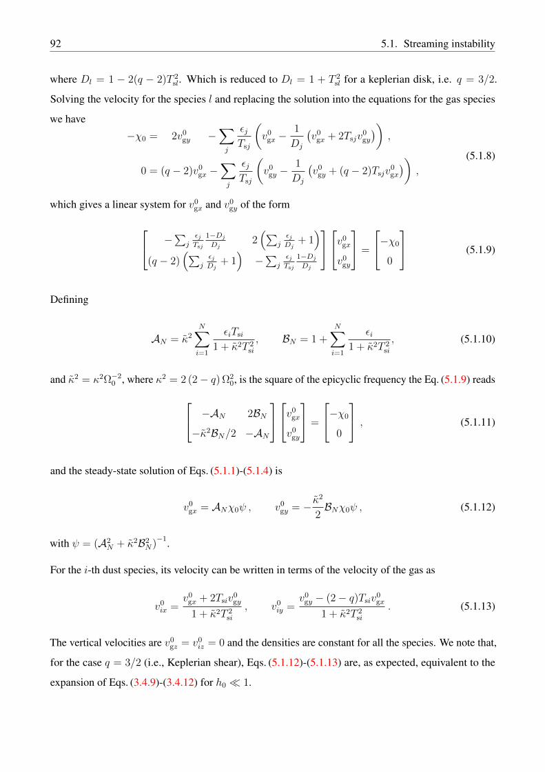
92 5.1. Streaming instability

where Dl = 1 − 2(q − 2)T 2sl. Which is reduced to Dl = 1 + T 2

sl for a keplerian disk, i.e. q = 3/2.

Solving the velocity for the species l and replacing the solution into the equations for the gas species

we have

−χ0 = 2v0gy −

∑

j

εjTsj

(v0

gx −1

Dj

(v0

gx + 2Tsjv0gy

)),

0 = (q − 2)v0gx −

∑

j

εjTsj

(v0

gy −1

Dj

(v0

gy + (q − 2)Tsjv0gx

)),

(5.1.8)

which gives a linear system for v0gx and v0

gy of the form

−∑j

εjTsj

1−Dj

Dj2(∑

jεjDj

+ 1)

(q − 2)(∑

jεjDj

+ 1)−∑j

εjTsj

1−Dj

Dj

v

0gx

v0gy

=

−χ0

0

(5.1.9)

Defining

AN = κ2

N∑

i=1

εiTsi

1 + κ2T 2si

, BN = 1 +N∑

i=1

εi1 + κ2T 2

si

, (5.1.10)

and κ2 = κ2Ω−20 , where κ2 = 2 (2− q) Ω2

0, is the square of the epicyclic frequency the Eq. (5.1.9) reads

−AN 2BN−κ2BN/2 −AN

v

0gx

v0gy

=

−χ0

0

, (5.1.11)

and the steady-state solution of Eqs. (5.1.1)-(5.1.4) is

v0gx = ANχ0ψ , v0

gy = − κ2

2BNχ0ψ , (5.1.12)

with ψ = (A2N + κ2B2

N)−1.

For the i-th dust species, its velocity can be written in terms of the velocity of the gas as

v0ix =

v0gx + 2Tsiv

0gy

1 + κ2T 2si

, v0iy =

v0gy − (2− q)Tsiv

0gx

1 + κ2T 2si

. (5.1.13)

The vertical velocities are v0gz = v0

iz = 0 and the densities are constant for all the species. We note that,

for the case q = 3/2 (i.e., Keplerian shear), Eqs. (5.1.12)-(5.1.13) are, as expected, equivalent to the

expansion of Eqs. (3.4.9)-(3.4.12) for h0 1.

5.1. Streaming instability 93

5.1.2 Linear regime - eigenvalues and eigenvectors

In this section, we linearize Eqs. (5.1.1)-(5.1.4) around the background solution (5.1.12)-(5.1.13) to

provide a framework for studying the stability of a given axisymmetric mode k = (kx, 0, kz).

Without loss of generality we assume perturbations of the form δf = Re(δfei(kxx+kzz)−ωt

).

Defining the dimensionless densities δρ = δρ/ρ0g, ε0k = ρ0

k/ρ0g, velocities v = v/(h2

0vK0), wavenumber

K = kh20vK0/Ω0, eigenvalue ω = ω/Ω0, and relative velocities ∆0

kx = v0gx − v0

kx, ∆0ky = v0

gy − v0ky,

the axisymmetric equations describing the linear evolution of the system are

iKxv0gxδρg + iKxδvgx + iKzδvgz = ωδρg

(iKxh

−20 −

N∑

k=1

ε0k∆0kx

Tsk

)δρg +

(iKxv

0gx +

N∑

k=1

ε0kTsk

)δvgx − 2δvgy +

N∑

k=1

∆0kx

Tskδρk −

N∑

k=1

ε0kTsk

δvkx = ωδvgx

−(

N∑

k=1

ε0k∆0ky

Tsk

)δρg + (2− q) δvgx +

(iKxv

0gx +

N∑

k=1

ε0kTsk

)δvgy +

N∑

k=1

∆0ky

Tskδρk −

N∑

k=1

ε0kTsk

δvky = ωδvgy

iKzh−20 δρg +

(iKxv

0gx +

N∑

k=1

ε0kTsk

)δvgz −

N∑

k=1

ε0kTsk

δvkz = ωδvgz

iKxv0jxδρj + iKxε

0jδvjx + iKzε

0jδvjz = ωδρj

− 1

Tsjδvgx +

(iKxv

0jx +

1

Tsj

)δvjx − 2δvjy = ωδvjx

− 1

Tsjδvgy + (2− q) δvjx +

(iKxv

0jx +

1

Tsj

)δvjy = ωδvjy

− 1

Tsjδvgz +

(iKxv

0jx +

1

Tsj

)δvjz = ωδvjz

(5.1.14)

A general expression for the dispersion relation and its eigenvectors can be easily obtained and written

in closed form (similar to what it was done in Section 3.3). However, due to the complexity of these

expressions, we avoid writing them here. Instead, for solving the eigenvalue problem we use the

function eig of NumPy (Walt et al., 2011), which uses LAPACK routines for complex non-symmetric

matrices (Anderson et al., 1999).

In Table 5.1.1 we present the parameters, the eigenvalues and the eigenvectors for the three different

cases, called LinA, LinB, and Lin3. The first two cases correspond to one gas and one dust species, and

have already been studied (e.g. Youdin and Johansen, 2007; Balsara et al., 2009; Bai and Stone, 2010b).

94 5.1. Streaming instability

Table 5.1.1: Table 4 from Benítez-Llambay et al. (2019). Eigenvalues, eigenvectors and parameters forthe runs LinA, LinB and Lin3

LinA LinB Lin3Parameters

K 30 6 50Ts1 0.1 0.1 0.0425ε1 3.0 0.2 1.0Ts2 – – 0.1ε2 – – 0.5

Eigenvalueω/Ω0 −0.4190091323 + 0.3480181522i −0.0154862262− 0.4998787515i −0.3027262829 + 0.3242790653i

Eigenvectorδρg +0.0000074637 + 0.0000070677i −0.0000337227− 0.0003456248i +0.0000061052 + 0.0000080743iδvgx −0.0563787907 + 0.0120535455i −0.0870451125− 1.3851731095i −0.1587288108 + 0.0213251096iδvgy +0.0445570113 + 0.0197224299i +1.3839936168− 0.0937424679i +0.1327989476 + 0.0674232641iδvgz +0.0563784989− 0.0120536242i +0.0870497444 + 1.3852113520i +0.1587286212− 0.0213252588iδv1x −0.0466198076 + 0.0124333223i +0.2314730923− 1.3715260043i −0.1461274403 + 0.0234873672iδv1y +0.0435211557 + 0.0213517453i +1.3696536978 + 0.0196879160i +0.1325843682 + 0.0691301709iδv1z +0.0546507401− 0.0077776652i +0.0416164539 + 1.3844311928i +0.1571142133− 0.0174328415iδρ2 – – +0.1522281314 + 0.1836379253iδv2x – – −0.1335593453 + 0.0025396632iδv2y – – +0.1092222067 + 0.0952973332iδv2z – – +0.1485545469 + 0.0200753935i

The dimensionless velocity amplitudes and wavenumber are defined as δv = δv/(h20vK0) and K = kh20vK0/Ω0,respectively. The dust-density perturbation δρ1 = 1 for all the runs.

The third one contains one gas and two dust species.

We report a small difference with respect to the eigenvalues obtained by Youdin and Johansen (2007).

We tracked down the difference to two terms in the linearized equations:

− δρg

N∑

k=1

ε0k∆0kx

Tsk

, and − δρg

N∑

k=1

ε0k∆0ky

Tsk

. (5.1.15)

Neglecting these terms modifies the fourth digit of the eigenvalues, and allows us to recover the values

reported by Youdin and Johansen (2007).

5.1.3 Linear regime - numerical solution

In this section, we study the numerical solution of the fully non-linear set of equations in the shearing-

box approximation. Simulations are performed with the shearing-box module of FARGO3D where dust

equations are solve using the scheme discussed in Chapter 3. We then compare the results with those

obtained from the linearized problem described in the previous section.

5.1. Streaming instability 95

0.0 7.6 15.2 22.8

Time

0.0

0.5

1.0

Den

sity

LinA

GAS

DUST1

DUST2

0.0 7.6 15.2 22.8

Time

0.0 7.6 15.2 22.8

Time

0.0

0.5

1.0

Den

sity

LinB

0.0 7.6 15.2 22.8

Time

0.0 7.6 15.2 22.8

Time

0.0

0.5

1.0

Den

sity

0.0 7.6 15.2 22.8

Time

Lin3

0.0 7.6 15.2 22.8

Time

101 102

N

10−8

10−7

10−6

10−5

Err

or

Slope = −2

LinA

LinB

Lin3

Figure 5.1.1: Figure 7 from Benítez-Llambay et al. (2019). Analytical (solid lines) and numerical(open circles) solutions of the linear streaming instability, for the runs LinA (top), LinB (center) andLin3 (bottom), obtained with 1282 grid points. From left to right, we plot the gas and dust densities.We additionally plot the result of the convergence test, described in Section 5.1.3.1. The agreementbetween the analytical and numerical solutions is excellent. The slope recovered from the convergencetest is consistent with the expected convergence rate for all the cases, showing small deviations for verylow resolutions.

The results presented in this section allow us to validate our framework and numerical methods to

further study the streaming instability including multiple species as well as the non-linear evolution, as

we will discuss in Sections 5.2 and 5.3.

To numerically recover the solutions we set h0 = 0.05 and vK0 = 1, and add the constant external force

χ0 to the gas component along the x direction. The shear parameter q is set to 3/2. We only consider

wavenumbers kx = kz = k, so we employ a square axisymmetric shearing-box with x, y ∈ [−L/2, L/2]

and L = 2π/k. The grid is evenly spaced over 256 cells in each direction. We set periodic and shear-

periodic boundary conditions in the z and x directions, respectively. The initial condition is given by

the steady-state background solution Eqs. (5.1.12) – (5.1.13), and we set the background densities to

96 5.1. Streaming instability

ρ0i = εiρ

0g, with ρ0

g = 1.0.

Because of truncation errors, the numerical equilibrium does not match to machine precision that given

by Eqs. (5.1.12)-(5.1.13). However, after initializing each run, the system rapidly relaxes towards an

exact numerical equilibrium. Thus, to improve our measurements, we wait for a time t0 = 1.2Ω−10 until

obtaining the numerical equilibrium. Then we excite the unstable mode. We note that to speed-up the

calculations, the relaxation step can be done in a 1D grid. We fix the CFL factor to 0.3 for all the runs.

The linear mode is excited by adding to the steady-state background the small perturbation δf , defined

Table 5.1.2: Table 5 from Benítez-Llambay et al. (2019). Measured growth rates for different numberof cells for the runs LinA, LinB and Lin3.

N LinA LinB Lin38 −0.325 ±3.3× 10−2 +0.030 ±1.2× 10−3 −0.222 ±8.5× 10−2

16 −0.3961 ±1.7× 10−3 −0.00821 ±2.9× 10−4 −0.271 ±4.9× 10−2

32 −0.41311 ±5.2× 10−4 −0.014468 ±7.3× 10−5 −0.291 ±1.3× 10−2

64 −0.41762 ±1.5× 10−4 −0.015349 ±2.2× 10−5 −0.3000 ±2.4× 10−3

128 −0.418583 ±8.0× 10−5 −0.0154688 ±6.5× 10−6 −0.30248 ±1.4× 10−4

256 −0.418900 ±5.4× 10−5 −0.0154839 ±2.0× 10−6 −0.302672 ±5.1× 10−5

The values correspond to the average of the growth rates obtained by fitting the time evolution of each component of theeigenvector. The errors correspond to the standard deviation of this average.

as:

δf = A[Re(δf)

cos(kxx+ kzz) − Im(δf)

sin(kxx+ kzz)], (5.1.16)

where δf is the complex amplitude of the corresponding component of the unstable eigenvector (see

Table 5.1.1) and A is a small amplitude that ensures linearity. Its value is set to A = 10−5.

In Figure 5.1.1, we plot the time evolution of the normalized density perturbations for each of the three

different cases, measured from time t0 at the location x = z = −L/2 (this is an arbitrary choice). In

the plot we adopt a normalization that sets the density perturbation between zero and one. In each

panel, we plot with open circles, the values obtained numerically with our implementation, while the

solid lines are the analytical ones. The color represents different species, blue being the gas and, orange

and red, the dust species. The first two rows of Figure 5.1.1 correspond to the tests LinA and LinB,

respectively. The third one corresponds to the three species Lin3 test. In all of the runs, the agreement

between the analytical and numerical solutions is excellent. We additionally comment that the same

level of agreement is observed for the velocities of the gas and the dust species.

In Table 5.1.2, we present the result of the measured growth rates for the tests LinA, LinB and Lin3, for

5.1. Streaming instability 97

different resolutions. The growth rate for each mode was obtained first by fitting each component of the

eigenvector and then averaging the results of the fits. For the tests LinA and Lin3, the instability can be

recovered with 8 cells. However, for the mode LinB, at least 16 cells are required to obtain an unstable

behavior. The errors correspond to the standard deviation of the average.

5.1.3.1 Linear regime - Convergence test

To test the convergence rate of these test problems, we perform a series of runs decreasing the resolutions

by factors of two, starting with 2562 cells down to 82 cells.

We measure the convergence rate for the three configurations described in the previous section by

computing the error, defined as

error =

(m∑

i=1

⟨(δf∆

i (t)− δfi(t))2⟩)1/2

, (5.1.17)

where m is the number of components of the eigenvector, δf∆ the numerical solution, δfi is the

analytical one, and 〈 〉 the time average between t = t0 and t = t0 + 7Ω−10 .

The rightmost large panel of Figure 5.1.1, shows the result of the convergence test for the three

different cases. We additionally plot (dashed line) the expected second-order accuracy slope. The

lowest resolution cases slightly depart from it. However, an excellent convergence rate is observed for

N > 322 grid points. The convergence properties for all the modes analyzed demonstrate the validity

of our implementation in agreement with the results presented in Chapter 3. It is remarkable that, even

with low resolution, our implementation is able to recover the linear growth rate with an acceptable

level of accuracy.

We report that we have observed the mode LinB to be prone to develop noise at cell level which,

eventually, contaminates the computational domain. By disabling the drag term, we have concluded that

this noise is something entirely related to the gas component. This issue was significantly reduced by

enabling a predictor using a half transport-step before the source step, allowing us to recover excellent

second-order accurate linear solutions (see Chapter 3 Section 3.2.3).

98 5.2. Streaming Instability for a Particle-Size Distribution

5.2 Streaming Instability for a Particle-Size Distribution

The linear phase of the Streaming Instability has been extensively studied including only one-dust

species (see e.g. Johansen and Youdin, 2007; Balsara et al., 2009; Kowalik et al., 2013; Chen and

Lin, 2018; Riols and Lesur, 2018). However, the dust component of PPDs may be characterized by

a non-trivial particle-size distribution (e.g., Birnstiel et al., 2012). In this section, we describe and

summarize the results obtained in Krapp et al. (2019), where we presented the first study of the linear

phase of the multispecies streaming instability. Our systematic exploration of parameter space allowed

us to provide the growth rate of the most unstable mode as a function of the dust-to-gas density ratio,

particle-size range, and number of dust species considered for describing a particle-size distribution a

we defined in Section 2.1.2.

5.2.1 Linear Modes in Fourier Space

The equations describing the dynamics of a gas coupled to N dust species via drag forces in the

framework of the shearing box, together with the analytical steady-state background solution, have been

presented in Section 5.1.1. Moreover, the linearized axisymmetric continuity and momentum equations

of 4(N+1) species where derived in Section 5.1.2 and validated in Section 5.1.3, where we successfully

recovered the linear growth of the streaming instability predicted by our analytical calculations. In

this section we study the stability of a given eigenmode that evolves in space and time according to

Re[δf(kx, kz) ei(kxx+kzz)−ωt]. Here, δf(kx, kz) are the 4(N + 1)-dimensional (complex) eigenvectors

in Fourier space, spanned by the wavenumbers (kx, kz), associated with the (complex) eigenvalue

ω(kx, kz). In the context of the streaming instability, it is customary to work with dimensionless

wavenumbers K = H20k/R0, where H0 is the disk sale-height at the fiducial radius R0, where the

shearing box is centered, and to use the Keplerian angular frequency, Ω0 ≡ ΩK(R0), to scale the

eigenvalues.

The early evolution of the instability is governed by the unstable modes – i.e., those with Re(ω) < 0 –

with maximum growth rate σ, given by

σ = max|Re(ω)| : Re(ω) < 0. (5.2.1)

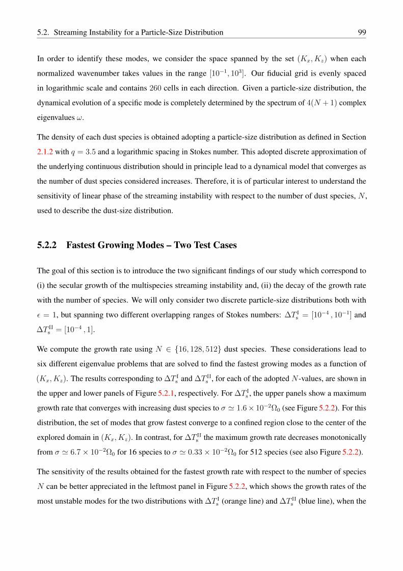
5.2. Streaming Instability for a Particle-Size Distribution 99

In order to identify these modes, we consider the space spanned by the set (Kx, Kz) when each

normalized wavenumber takes values in the range [10−1, 103]. Our fiducial grid is evenly spaced

in logarithmic scale and contains 260 cells in each direction. Given a particle-size distribution, the

dynamical evolution of a specific mode is completely determined by the spectrum of 4(N + 1) complex

eigenvalues ω.

The density of each dust species is obtained adopting a particle-size distribution as defined in Section

2.1.2 with q = 3.5 and a logarithmic spacing in Stokes number. This adopted discrete approximation of

the underlying continuous distribution should in principle lead to a dynamical model that converges as

the number of dust species considered increases. Therefore, it is of particular interest to understand the

sensitivity of linear phase of the streaming instability with respect to the number of dust species, N ,

used to describe the dust-size distribution.

5.2.2 Fastest Growing Modes – Two Test Cases

The goal of this section is to introduce the two significant findings of our study which correspond to

(i) the secular growth of the multispecies streaming instability and, (ii) the decay of the growth rate

with the number of species. We will only consider two discrete particle-size distributions both with

ε = 1, but spanning two different overlapping ranges of Stokes numbers: ∆T Is = [10−4 , 10−1] and

∆T IIs = [10−4 , 1].

We compute the growth rate using N ∈ 16, 128, 512 dust species. These considerations lead to

six different eigenvalue problems that are solved to find the fastest growing modes as a function of

(Kx, Kz). The results corresponding to ∆T Is and ∆T II

s , for each of the adopted N -values, are shown in

the upper and lower panels of Figure 5.2.1, respectively. For ∆T Is , the upper panels show a maximum

growth rate that converges with increasing dust species to σ ' 1.6× 10−2Ω0 (see Figure 5.2.2). For this

distribution, the set of modes that grow fastest converge to a confined region close to the center of the

explored domain in (Kx, Kz). In contrast, for ∆T IIs the maximum growth rate decreases monotonically

from σ ' 6.7× 10−2Ω0 for 16 species to σ ' 0.33× 10−2Ω0 for 512 species (see also Figure 5.2.2).

The sensitivity of the results obtained for the fastest growth rate with respect to the number of species

N can be better appreciated in the leftmost panel in Figure 5.2.2, which shows the growth rates of the

most unstable modes for the two distributions with ∆T Is (orange line) and ∆T II

s (blue line), when the

100 5.2. Streaming Instability for a Particle-Size Distribution

Figure 5.2.1: Figure 1 from Krapp et al. (2019). Color map displaying the growth rate σ of the mostunstable mode for the multi-species streaming instability as a function of the wavenumbers Kx andKz. Results are shown for two number-density distributions with power-law of index q = −3.5 in theparticle-size/Stokes number and equal dust-to-gas mass ratio, ε = 1, for Stokes numbers logarithmicallyspaced in ∆T I

s = [10−4 , 10−1] (upper panels) and ∆T IIs = [10−4 , 1] (lower panels) and for an increasing

number of dust species N = 16, 128, 512. Dashed lines denoting σ = 10−3Ω0, mark the turning pointof the divergent color palette. Hatched regions are stable. White triangles correspond to the fastestgrowing modes whose temporal evolution we checked independently using the code FARGO3D (seeFig. 5.2.2).

number of dust species doubles from N = 2 to N = 2048. For the case ∆T Is the maximum growth rate

converges when using 64 dust species. This is not the case for ∆T IIs , for which the maximum growth

rate decreases below σ < 10−3Ω0. However, in a region around Kx = 10−1, the growth rate converges

to ∼ 5 × 10−4Ω0 for N ≥ 64. This value sets the time scale of the linear instability for N > 2048

species.

In order to shed some light on the strikingly different behaviour exhibited by ∆T I and ∆T II, we show

in Figure 5.2.3 high resolution maps in (Kx, Kz) zooming-in the neighborhood of the fastest growing

modes. The left and right panels show the maximum growth rate for 64 and 128 species, respectively.

The upper and lower panels correspond to ∆T Is and ∆T II

s (orange and blue curves in Figure 5.2.2),

5.2. Streaming Instability for a Particle-Size Distribution 101

I

II

II

I

Figure 5.2.2: Figure 2 from Krapp et al. (2019). Real (left panel) and imaginary (middle panel)parts for the eigenvalues corresponding to the most unstable modes for the particle distributions withdust-to-gas mass ratio ε = 1 and Stokes numbers in the intervals ∆T I

s = [10−4 , 10−1] (orange) and∆T II

s = [10−4 , 1] (blue) as a function of particle species number N . The two rightmost panels show thetime evolution of the density fluctuation of dust species 1, δρ1, for the most unstable eigenmode. Redand green unfilled circles show the solutions obtained with FARGO3D for 16 and 128 dust-species,respectively, using 32 cells per wavelength. The solid black lines correspond to the solutions of thelinear mode analysis described in Section 5.2.1.

respectively. These maps reveal a pattern with a number of fringes that increases linearly with N , as

they split unstable regions for which the growth rates also decay also linearly with N . If these fringes

merge, i.e., their separation is smaller than their width, the growth rates converge. It is worth stressing

that the imaginary parts corresponding to the most unstable eigenvalues (shown in the middle panel of

Figure 5.2.2) do converge as N increases in both cases. Because only the real part of the eigenvalue

varies with the number of species, the decay seems to be an intrinsic property of the instability rather

than systematic errors introduced in our method.

The decay observed in the growth rate of the most unstable modes when N increases in the case ∆T IIs

is in stark contrast with the behavior observed for ∆T Is . This warrants a systematic exploration of

parameter space including also the dust-to-gas mass ratio. Before embarking on this, and given the

complexity of the equations involved in the linear mode analysis describing the multi-species streaming

instability, we provide an independent check of our solutions below.

5.2.3 Verification of the Linear Mode Analysis

We test the time evolution of the most unstable modes following the procedure described in Section

5.1.3. We consider four representative cases from Figure 5.2.2 (red and green filled circles) and use the

corresponding eigenvectors to initialize four numerical simulations. The rightmost panels of Figure 5.2.2

102 5.2. Streaming Instability for a Particle-Size Distribution

15 20 25 305

7

9

11

13

Kz

15 20 25 30

2.5 3.0 3.5

Kx

65.0

67.5

70.0

72.5

75.0

Kz

2.5 3.0 3.5

Kx

0.5 1.6σ

0.5 1.6σ

2.20 2.36σ

1.20 1.26σ

Figure 5.2.3: Figure 3 from Krapp et al. (2019). High-resolution maps of the normalized growth rateσ = 102σ/Ω0. Zoom-in domains surrounding the fastest growing modes for the distributions withStokes numbers in ∆T I

s = [10−4 , 10−1] and ∆T IIs = [10−4 , 1] (upper and lower panels, respectively)

for N = 64 and 128 species (left and right panels, respectively).

show the time evolution for one of the components (the dust density for species 1, δρ1) for each of these

four modes. The solutions obtained with FARGO3D are shown with red and green unfilled circles for

16 and 128 dust-species, respectively. The black solid lines are the solutions obtained from our linear

mode analysis described in Section 5.2.1. A detailed comparison between the analytical and numerical

solutions of the density and velocity components of all the species is presented in Appendix A.3. The

excellent agreement between the time evolution of the selected eigenmodes provides additional support

to our linear calculations. This critically reduces the possibility of potential issues in several steps of

our analysis including the derivation of the background equilibrium, the linearization of the perturbed

system, and the method used to find the eigenvalues and eigenvectors.

5.2.4 Systematic Parameter Space Exploration

We seek the growth rate of the most unstable mode given a particle-size distribution characterized

by the dust-to-gas mass ratio, ε, a range of Stokes numbers, ∆Ts = [Ts,min, Ts,max], and the total

number of species N . We consider four different mass ratios, ε = 0.01, 0.1, 0.5, 1 and two sets

of intervals in Stokes numbers for which either the minimum is fixed and the maximum varies,

5.2. Streaming Instability for a Particle-Size Distribution 103

i.e., ∆Ts,min = [10−4, Ts,max] with Ts,max ∈ 10−3, 10−2, 10−1, 1, or the maximum is fixed and the

minimum varies, i.e., ∆Ts,max = [Ts,min, 1] with Ts,min = 10−1, 10−2, 10−3, 10−4. For each of these

intervals in Stokes numbers, we consider an increasing number of dust-species by doubling N from 2 to

2048 while keeping the dust-to-gas mass ratio characterizing the distribution constant. This procedure

leads to 4× (4× 2− 1)× 11 = 308 independent discrete distributions.

I II

Figure 5.2.4: Figure 4 from Krapp et al. (2019). Maximum growth rate for the multi-species streaminginstability as a function of the number of the dust-species N for different ranges of Stokes numbers and(fixed) dust-to-gas mass ratio, from left to right each block corresponds to ε = 0.01, 0.1, 0.5, 1. Theupper panels show the results when considering a fixed Ts,min = 10−4 and varying Ts,max. The lowerpanels show the results when considering a fixed Ts,max = 1 and varying Ts,min. The green circles, ineach panel, show examples of distributions that have the same number of species per decade in Stokesnumber. White triangles are used to indicate the correspondence with the distributions used to computethe growth rate maps in Figure 5.2.1.

The maximum growth rates for each of the distributions defined above are shown in Figure 5.2.4. Each

panel corresponds to a different dust-to-gas mass ratio ε. The rows and columns correspond to a given

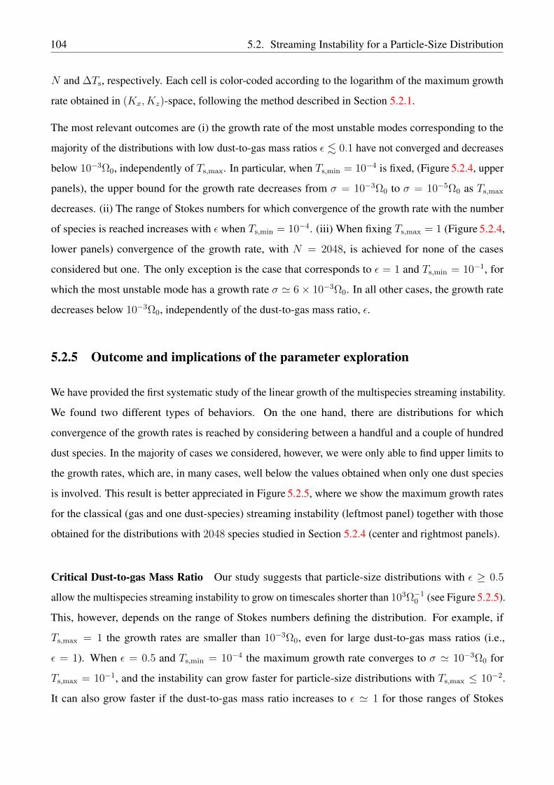
104 5.2. Streaming Instability for a Particle-Size Distribution

N and ∆Ts, respectively. Each cell is color-coded according to the logarithm of the maximum growth

rate obtained in (Kx, Kz)-space, following the method described in Section 5.2.1.

The most relevant outcomes are (i) the growth rate of the most unstable modes corresponding to the

majority of the distributions with low dust-to-gas mass ratios ε . 0.1 have not converged and decreases

below 10−3Ω0, independently of Ts,max. In particular, when Ts,min = 10−4 is fixed, (Figure 5.2.4, upper

panels), the upper bound for the growth rate decreases from σ = 10−3Ω0 to σ = 10−5Ω0 as Ts,max

decreases. (ii) The range of Stokes numbers for which convergence of the growth rate with the number

of species is reached increases with ε when Ts,min = 10−4. (iii) When fixing Ts,max = 1 (Figure 5.2.4,

lower panels) convergence of the growth rate, with N = 2048, is achieved for none of the cases

considered but one. The only exception is the case that corresponds to ε = 1 and Ts,min = 10−1, for

which the most unstable mode has a growth rate σ ' 6× 10−3Ω0. In all other cases, the growth rate

decreases below 10−3Ω0, independently of the dust-to-gas mass ratio, ε.

5.2.5 Outcome and implications of the parameter exploration

We have provided the first systematic study of the linear growth of the multispecies streaming instability.

We found two different types of behaviors. On the one hand, there are distributions for which

convergence of the growth rates is reached by considering between a handful and a couple of hundred

dust species. In the majority of cases we considered, however, we were only able to find upper limits to

the growth rates, which are, in many cases, well below the values obtained when only one dust species

is involved. This result is better appreciated in Figure 5.2.5, where we show the maximum growth rates

for the classical (gas and one dust-species) streaming instability (leftmost panel) together with those

obtained for the distributions with 2048 species studied in Section 5.2.4 (center and rightmost panels).

Critical Dust-to-gas Mass Ratio Our study suggests that particle-size distributions with ε ≥ 0.5

allow the multispecies streaming instability to grow on timescales shorter than 103Ω−10 (see Figure 5.2.5).

This, however, depends on the range of Stokes numbers defining the distribution. For example, if

Ts,max = 1 the growth rates are smaller than 10−3Ω0, even for large dust-to-gas mass ratios (i.e.,

ε = 1). When ε = 0.5 and Ts,min = 10−4 the maximum growth rate converges to σ ' 10−3Ω0 for

Ts,max = 10−1, and the instability can grow faster for particle-size distributions with Ts,max ≤ 10−2.

It can also grow faster if the dust-to-gas mass ratio increases to ε ' 1 for those ranges of Stokes

5.2. Streaming Instability for a Particle-Size Distribution 105

10−4 10−3 10−2 10−1 100

Ts

10−2

10−1

100

ε

Two fluids

10−3 10−2 10−1 100

Ts,max

Particle-size distribution

10−410−310−210−1

Ts,min

Particle-size distribution

−6 −5 −4 −3 −2 −1 0

log10 (σ/Ω0)

Figure 5.2.5: The left panel shows the maximum growth rate corresponding to the classical streaminginstability involving only one dust-species. The center and rightmost panel show the maximum growthrate obtained for distributions with 2048 species when fixing Ts,min = 10−4 and Ts,max = 1, respectively.The dashed line corresponds to σ = 10−3Ω0 in all panels.

numbers. We additionally found that, if the total mass of the distribution decreases below ε = 0.5, the

instability develops on timescales of the order of 105Ω−10 , or even longer, depending on the range of

Stokes numbers spanned by the particle distribution.

Simulations of Multi-Species Streaming Instability The successful recovery of known solutions is

a key benchmark for any numerical code. Previous numerical studies of the non-linear evolution of the

streaming instability with one dust species have been reported to recover, for example, its linear phase

(see e.g. Johansen and Youdin, 2007; Balsara et al., 2009; Kowalik et al., 2013; Chen and Lin, 2018;

Riols and Lesur, 2018; Benítez-Llambay et al., 2019). Even though the linear results have been derived

using an Eulerian formalism, it has been shown that numerical codes evolving Lagrangian particles

agree very well during the early phases of the streaming instability (Youdin and Johansen, 2007). This

suggests that our findings will also hold in the Lagrangian framework. It is possible that a significant

decay of the growth rate has not yet been observed in multiple dust-species simulations because of the

relatively low number of species that have been used so far (see e.g. Bai and Stone, 2010b; Schaffer

et al., 2018).

Single-dust Species Models of Streaming Instability We report the emergence of an unstable region

for Kx 1 and Kz ≥ 0, which has not been observed before (see Youdin and Goodman, 2005; Youdin

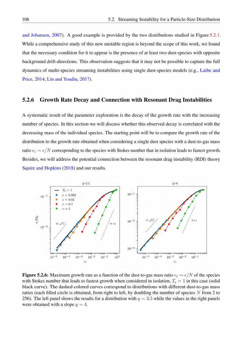
106 5.2. Streaming Instability for a Particle-Size Distribution

and Johansen, 2007). A good example is provided by the two distributions studied in Figure 5.2.1.

While a comprehensive study of this new unstable region is beyond the scope of this work, we found

that the necessary condition for it to appear is the presence of at least two dust-species with opposite

background drift-directions. This observation suggests that it may not be possible to capture the full

dynamics of multi-species streaming instabilities using single dust-species models (e.g., Laibe and

Price, 2014; Lin and Youdin, 2017).

5.2.6 Growth Rate Decay and Connection with Resonant Drag Instabilities

A systematic result of the parameter exploration is the decay of the growth rate with the increasing

number of species. In this section we will discuss whether this observed decay is correlated with the

decreasing mass of the individual species. The starting point will be to compare the growth rate of the

distribution to the growth rate obtained when considering a single dust species with a dust-to-gas mass

ratio ε1 ∼ ε/N corresponding to the species with Stokes number that in isolation leads to fastest growth.

Besides, we will address the potential connection between the resonant drag instability (RDI) theory

Squire and Hopkins (2018) and our results.

q=3.5 q=4r

Figure 5.2.6: Maximum growth rate as a function of the dust-to-gas mass ratio ε1 ∼ ε/N of the specieswith Stokes number that leads to fastest growth when considered in isolation, Ts = 1 in this case (solidblack curve). The dashed colored curves correspond to distributions with different dust-to-gas massratios (each filled circle is obtained, from right to left, by doubling the number of species N from 2 to256). The left panel shows the results for a distribution with q = 3.5 while the values in the right panelswere obtained with a slope q = 4.

5.2. Streaming Instability for a Particle-Size Distribution 107

We consider two distribution in a range of Stokes number [10−4, 1] that differ in the adopted slopes,

q = 3.5 and q = 4, respectively. Figure 5.2.6 shows the results of the comparison. The black solid line

correspond to the growth rate of two-fluid problem obtained considering an species with Ts = 1 and a

dust-to-gas density ratio ε1, obtained from the distribution.

We found that for ε < 10−2 the maximum growth rate of the distribution is in good agreement with

the value obtained when considering in isolation the species with largest Stokes number. However, as

the total mass of the distribution considered is increased, a significant difference between these growth

rates exists. This is due to two effects that are difficult to disentangle; i) the background drift-velocity

for each individual dust-species is modified because it is sensitive to the total mass of the particle-size

distribution and not just the mass per bin (see Section 5.1.1) and ii) as the ensuing gas perturbation

increases, the coupling between species increases and interference among them may not be negligible.

It seems that in the regime where ε < 10−2, the resonant drag instability (RDI) framework (Squire and

Hopkins, 2018) can help to provide insight into the behavior of the multispecies streaming instability. At

sufficiently low dust-to-gas mass ratios the maximum growth rate is expected to decay as√ε1 ∼

√ε/N .

This is indeed obtained for distributions with dust-to-gas mass ratios smaller than ε = 0.01 (see

Figure 5.2.6).

The connection between the multiple species streaming instability and the RDI can be better appreciated

in Figure 5.2.7, where we show the stability maps (equivalent to the maps in Figure 5.2.1) for two

distributions. Each distribution has eight species with a dust-to-gas mass ratio of ε = 10−5 (upper panel)

and ε = 1 (lower panel). The left panels in each of these figures show the maps of the growth rate

for the multi-fluid system. On top of the maps, we over plot with dashed lines each of the normalized

resonant wavenumbers, (Kx,i, 0, Kz,i), solution of the equation (see Squire and Hopkins, 2018, Eq. 30)

Kx,i(v0gx − v0

dx,i) =Kz,i√

K2x,i +K2

z,i

Ω0 , with i = 1, . . . , 8 , (5.2.2)

where Kz, Kx, Ω0, v0gx and v0

dx,i where defined in Section 5.1.3.

Right panels of Figure 5.2.7 show a 1-dimensional cut of the left panels at those vertical wavenumbers

where the local maxima of the multi-species system are found (solid black line) together with the

corresponding results obtained for the single dust-species configurations (dashed colored lines).

In the limit of very low mass, the multi-species streaming instability can be well described as the

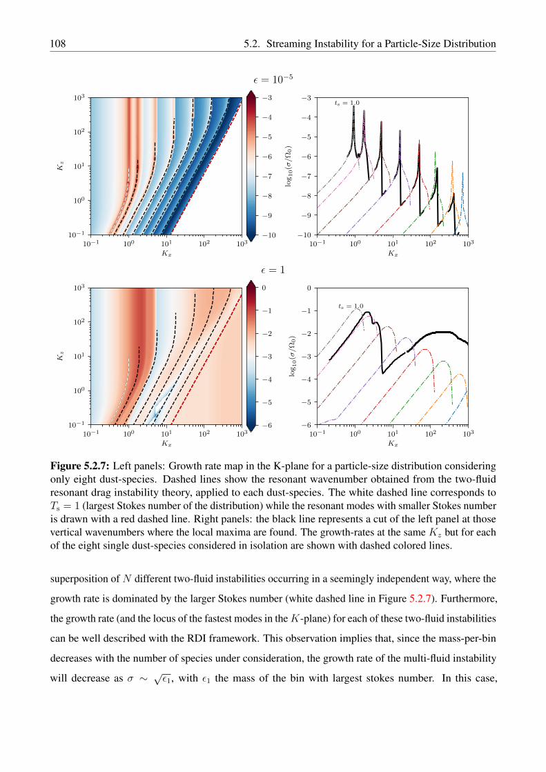
108 5.2. Streaming Instability for a Particle-Size Distribution

10−1 100 101 102 103

Kx

10−1

100

101

102

103

Kz

10−1 100 101 102 103

Kx

−10

−9

−8

−7

−6

−5

−4

−3

log

10(σ/Ω

0)

ts = 1.0

−10

−9

−8

−7

−6

−5

−4

−3

ε = 10−5

10−1 100 101 102 103

Kx

10−1

100

101

102

103

Kz

10−1 100 101 102 103

Kx

−6

−5

−4

−3

−2

−1

0lo

g10(σ/Ω

0)

ts = 1.0

−6

−5

−4

−3

−2

−1

0

ε = 1

Figure 5.2.7: Left panels: Growth rate map in the K-plane for a particle-size distribution consideringonly eight dust-species. Dashed lines show the resonant wavenumber obtained from the two-fluidresonant drag instability theory, applied to each dust-species. The white dashed line corresponds toTs = 1 (largest Stokes number of the distribution) while the resonant modes with smaller Stokes numberis drawn with a red dashed line. Right panels: the black line represents a cut of the left panel at thosevertical wavenumbers where the local maxima are found. The growth-rates at the same Kz but for eachof the eight single dust-species considered in isolation are shown with dashed colored lines.

superposition of N different two-fluid instabilities occurring in a seemingly independent way, where the

growth rate is dominated by the larger Stokes number (white dashed line in Figure 5.2.7). Furthermore,

the growth rate (and the locus of the fastest modes in theK-plane) for each of these two-fluid instabilities

can be well described with the RDI framework. This observation implies that, since the mass-per-bin

decreases with the number of species under consideration, the growth rate of the multi-fluid instability

will decrease as σ ∼ √ε1, with ε1 the mass of the bin with largest stokes number. In this case,

5.3. Non-linear evolution of the Streaming Instability 109

the convergence of the growth rate as the number of species increases is, for obvious reasons, not

guaranteed.

As the mass of the distribution increases, the naive superposition of two-fluid instabilities does not

work anymore. However, even for such a large mass, it is interesting to note that one could arbitrarily

increase the number of species to obtain a mass-per-bin arbitrarily small, where the RDI theory could

be, in principle, applied to each mass bin. Nevertheless, this is not strictly true because the background

velocities do depend on the total mass of the distribution but not on the individual mass-per-bin.

Furthermore, as shown in Figure 5.2.6, for the dust-to-gas mass ratio ε > 0.01 the growth rate associated

with particle distributions decreases proportionally to the number of species (or mass-per-bin), which

might be due to the non-trivial feedback between several subdominant species.

5.3 Non-linear evolution of the Streaming Instability

As we concluded in the previous section, if dust-to-gas mass ratios are larger than ε > 0.5 or segregation

mechanisms induce a monodisperse population of dust, the streaming instability might be a natural

outcome of the aerodynamic coupling between gas and dust. Understanding the non-linear evolution of

the streaming instability and its consequences still represent a challenge, and numerical simulations

seems good candidates to tackle the problem. Motivated by the reduced number of simulations where

dust is treated as a pressureless fluid and the benefits of our numerical implementation (see Chapter 3

for a discussion ), we dedicate this section to study previous results where the dust was simulated using

Lagrangian particles. We discuss the advantages of our approach, together with the major discrepancies.

We consider the runs AB and BA described by Johansen and Youdin (2007) and Bai and Stone (2010b).

We focus our attention on the convergence with resolution, the cumulative dust density distribution

and the time evolution of the maximum density. These tests give us, in particular, the opportunity to

assess whether the Eulerian approach for the dust species is able to reproduce similar features as those

obtained by Bai and Stone (2010b) using Lagrangian particles.

For each test, we set a square shearing-box of size L = lh0H0, with h0 = 0.05, H0 = h0R0, and the

fiducial radius R0 = 1. The shear parameter q is, as above, 3/2 (i.e., Keplerian rotation). For the test

AB (BA), we set the dust-to-gas mass ratio ε1 = 1 (ε1 = 0.2), the Stokes number Ts1 = 0.1 (Ts1 = 1.0),

110 5.3. Non-linear evolution of the Streaming Instability

1282 2562 5122

10242 20482 40962

−1.00 −0.75 −0.50 −0.25 0.00 0.25 0.50 0.75 1.00

log10 (ρd)

Figure 5.3.1: Figure 8 from Benítez-Llambay et al. (2019) Dust density maps for the test AB. Eachpanel is labeled by the total number of cells of the box. This mode is dominated by over-dense filamentsand voids. The larger the resolution, the smaller and denser the filaments become. Convergence withresolution is far from being observed for the resolutions studied. The panels corresponding to 2562

and 10242 cells can be compared with Figure 5 of Bai and Stone (2010b), where a good qualitativeagreement is observed.

and the parameter l = 2 (l = 40). The total integration time is set to 40Ω−10 (800Ω−1

0 ), which allows the

saturated turbulent state to be reached (Bai and Stone, 2010b). We seed the instability with white noise

in the three velocity components of the two species, with an amplitude A = 10−2h0vK0.

To test convergence with resolution, for a fixed box size, we vary the number of grid cells by a factor

of four. For the test BA, we set the nominal box with 642 cells – a resolution of roughly 32/H0 – and

obtain results when varying the number of cells up to 20482 – a resolution of 1024/H0. For the test

AB, since a box with 642 cells does not allow the instability to growth, we start with 1282 cells – a

resolution of 1280/H0 – and increase it up to 40962 cells – a resolution of 40960/H0. We note that,

when using 642 cells for the run AB, Bai and Stone (2010b) were able to recover an unstable evolution,

which is probably due to the higher order of the Athena code. For the run AB, and the lowest resolution

(1282 grid cells), we report a saturation time ' 12Ω−10 , a value higly dependent on resolution. On the

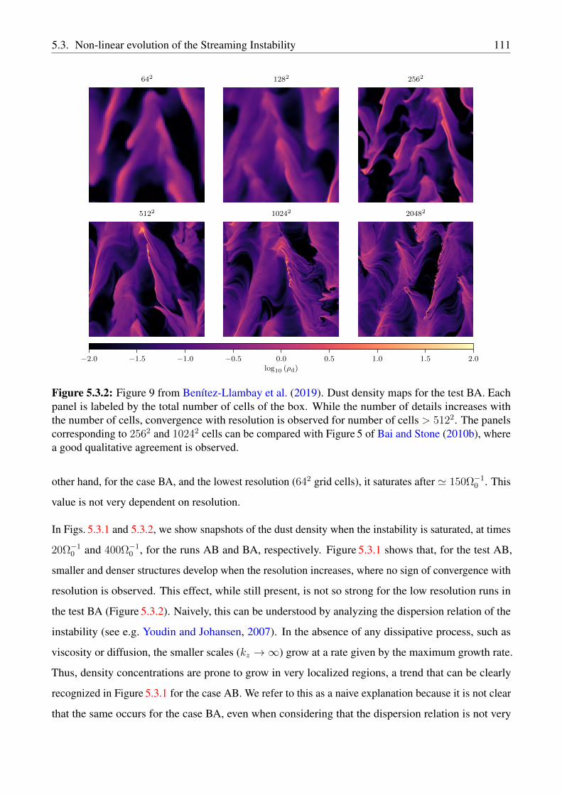
5.3. Non-linear evolution of the Streaming Instability 111

642 1282 2562

5122 10242 20482

−2.0 −1.5 −1.0 −0.5 0.0 0.5 1.0 1.5 2.0

log10 (ρd)

Figure 5.3.2: Figure 9 from Benítez-Llambay et al. (2019). Dust density maps for the test BA. Eachpanel is labeled by the total number of cells of the box. While the number of details increases withthe number of cells, convergence with resolution is observed for number of cells > 5122. The panelscorresponding to 2562 and 10242 cells can be compared with Figure 5 of Bai and Stone (2010b), wherea good qualitative agreement is observed.

other hand, for the case BA, and the lowest resolution (642 grid cells), it saturates after ' 150Ω−10 . This

value is not very dependent on resolution.

In Figs. 5.3.1 and 5.3.2, we show snapshots of the dust density when the instability is saturated, at times

20Ω−10 and 400Ω−1

0 , for the runs AB and BA, respectively. Figure 5.3.1 shows that, for the test AB,

smaller and denser structures develop when the resolution increases, where no sign of convergence with

resolution is observed. This effect, while still present, is not so strong for the low resolution runs in

the test BA (Figure 5.3.2). Naively, this can be understood by analyzing the dispersion relation of the

instability (see e.g. Youdin and Johansen, 2007). In the absence of any dissipative process, such as

viscosity or diffusion, the smaller scales (kz →∞) grow at a rate given by the maximum growth rate.

Thus, density concentrations are prone to grow in very localized regions, a trend that can be clearly

recognized in Figure 5.3.1 for the case AB. We refer to this as a naive explanation because it is not clear

that the same occurs for the case BA, even when considering that the dispersion relation is not very

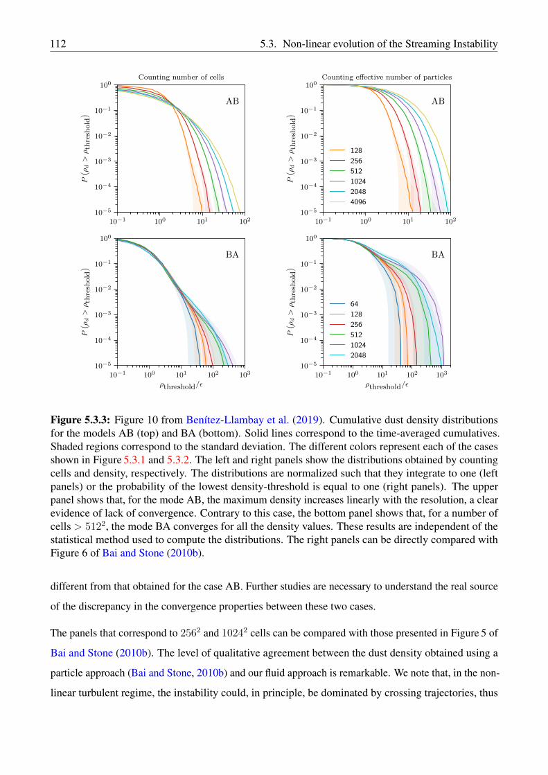
112 5.3. Non-linear evolution of the Streaming Instability

10−1 100 101 10210−5

10−4

10−3

10−2

10−1

100P( ρd>ρth

resh

old)

AB

Counting number of cells

10−1 100 101 10210−5

10−4

10−3

10−2

10−1

100

P( ρd>ρth

resh

old)

AB

Counting effective number of particles

128

256

512

1024

2048

4096

10−1 100 101 102 103

ρthreshold/ε

10−5

10−4

10−3

10−2

10−1

100

P( ρd>ρth

resh

old)

BA

10−1 100 101 102 103

ρthreshold/ε

10−5

10−4

10−3

10−2

10−1

100

P( ρd>ρth

resh

old)

BA

64

128

256

512

1024

2048

Figure 5.3.3: Figure 10 from Benítez-Llambay et al. (2019). Cumulative dust density distributionsfor the models AB (top) and BA (bottom). Solid lines correspond to the time-averaged cumulatives.Shaded regions correspond to the standard deviation. The different colors represent each of the casesshown in Figure 5.3.1 and 5.3.2. The left and right panels show the distributions obtained by countingcells and density, respectively. The distributions are normalized such that they integrate to one (leftpanels) or the probability of the lowest density-threshold is equal to one (right panels). The upperpanel shows that, for the mode AB, the maximum density increases linearly with the resolution, a clearevidence of lack of convergence. Contrary to this case, the bottom panel shows that, for a number ofcells > 5122, the mode BA converges for all the density values. These results are independent of thestatistical method used to compute the distributions. The right panels can be directly compared withFigure 6 of Bai and Stone (2010b).

different from that obtained for the case AB. Further studies are necessary to understand the real source

of the discrepancy in the convergence properties between these two cases.

The panels that correspond to 2562 and 10242 cells can be compared with those presented in Figure 5 of

Bai and Stone (2010b). The level of qualitative agreement between the dust density obtained using a

particle approach (Bai and Stone, 2010b) and our fluid approach is remarkable. We note that, in the non-

linear turbulent regime, the instability could, in principle, be dominated by crossing trajectories, thus

5.3. Non-linear evolution of the Streaming Instability 113

invalidating our approach. However, the overall agreement obtained from this qualitative comparison

suggests that the dynamics of the instability, in the non-linear regime, could be treated using a fluid

approach.

To better quantify the convergence properties for both the AB and BA tests, following Youdin and

Johansen (2007) and Bai and Stone (2010b), we study the cumulative dust-density distribution. We

calculate it by following two different procedures, one by the counting number of cells with density

above some threshold value, ρthreshold, and another one by adding up the density of cells with density

above ρthreshold. The latter is similar to counting (the effective) number of particles, as done by Youdin

and Johansen (2007) and Bai and Stone (2010b). We split the dust density in 300 logarithmic bins,

between log10(ρaε) and log10(ρbε), where ρb = 102 for the case AB, while ρb = 2 × 103 for BA,

and ρa = 10−1 in both cases. To obtain a representative cumulative function of the saturated regime,

we compute it for different times, between t = 30Ω−10 and t = 600Ω−1

0 for the cases AB and BA,

respectively, until the final integration time, and we finally average them. We also compute the standard

deviation, which provides valuable information about the fluctuations of the density in the saturated

phase.

In Figure 5.3.3 we plot the time averaged cumulative distributions for the dust density, corresponding

to the cases AB (upper panels) and BA (lower panels). In each panel, and with different colors, we

plot the cumulative function corresponding to the data shown in the panels of Figure 5.3.1 and 5.3.2.

Shaded regions show the standard deviation. The left and right panels show the results obtained by

counting the number of cells and by summing the density of the cells, respectively. In the left panels,

the distributions are normalized such that they integrate to one. For comparative purposes with Bai and

Stone (2010b), the curves in the right panels are normalized such that the probability of the minimum

density bin is one.

For both cases, AB and BA, the dispersion is very small and does not depend on the method used to

calculate the cumulative distribution. In particular, for the run BA, a strong degree of convergence,

down to probabilities of the order P (ρd > ρthreshold) ∼ 10−3 is observed for all the resolutions. We

report that, for P = 10−5, the obtained probabilities correspond to values of ρthreshold/ε that are roughly

one order of magnitude below the values presented by Bai and Stone (2010b) when counting number

of cells. However, counting (the effective) number of particles, by adding up densities, removes this

discrepancy. Contrary to what is observed for the case AB, the mode BA seems converged for a number

114 5.3. Non-linear evolution of the Streaming Instability

of cells larger than 5122.

0 10 20 30 40

Time

10−1

100

101

102

103

max

(ρd/ε)

AB

128

256

512

1024

2048

4096

0 200 400 600 800

Time

100

101

102

103

max

(ρd/ε)

BA

64

128

256

512

1024

2048

Figure 5.3.4: Figure 11 from Benítez-Llambay et al. (2019). Maximum dust density over time forthe modes AB (left panel) and BA (right panel). As shown in Figure 5.3.3, the maximum density forthe case AB increases linearly with resolution. The left panel also shows that the time for saturationis directly correlated with the resolution. Contrary to this case, the mode BA presents much betterconvergence properties with resolution. The right panel shows that, for low resolution, the initial growthrate directly correlates with resolution. However, for number of cells > 5122, convergence in the growthrate is observed. The same degree of convergence is observed for the maximum dust density over thetime interval considered, where both the maximum and fluctuations are comparable.

The method used to calculate the cumulative distributions does not modify the degree of convergence

found for each run, AB and BA. However, the shape of the distributions is method-dependent. When

counting cells, lower densities contribute more significantly in shaping the cumulative distribution,

while when counting (the effective) number of particles, denser regions contribute more. While the

maximum-density values differ from those obtained by Bai and Stone (2010b) for the run AB, the

overall shape of the distributions agrees better when adding up densities.

The run AB shows a direct correlation between the saturation time scale and the resolution, i.e., the

higher the resolution, the faster the instability saturates. Furthermore, we find the maximum density to

be proportional to the number of cells, a clear evidence of lack of convergence. The previous analysis is

supported by Figure 5.3.4, where we plot the maximum dust density as a function of time for each case

and resolution. As described above, we show again that the run BA is much better behaved in terms of

convergence. While the maximum density also increases with resolution for the low resolution cases, it

converges when using more than 5122 cells.

5.4. Summary and Conclusions 115

The differences found when comparing our results with those obtained using Lagrangian particles, in

particular the lack of convergence for the run AB, warrant a detailed comparison between these two

approaches.

5.4 Summary and Conclusions

Framework for linear theory. We derived the steady-state analytical solutions in a shearing-box

approximation using an external force to mimic the pressure gradient within the disk. We linearized the

equations assuming axisymmetric perturbations to study the time evolution of unstable modes. The

obtained analytical solutions were recovered numerically by solving the full non-linear fluid equations

with FARGO3D considering 1, 2, 16, and 128 dust species. These results validate both our numerical

implementation discussed in Chapter 3 and our analytical framework.

Linear streaming instability for a particle size-distribution. We presented the first systematic

study of the linear phase of the streaming instability, including multiple dust species. We considered

power-law particle-size distributions with different ranges of Stokes numbers and dust-to-gas density

ratios. The growth rate for the distribution with ε & 0.5 are similar to those obtained for the two-fluid

problem, except for the distribution with small Stokes numbers, i.e., Ts,max < 10−2, where the instability

grows on timescales much faster in comparison with the two-fluid case. Convergence of the linear

phase is reached for system with less than 100 species. Contrary to these cases, when ε < 0.5 the

timescale of the instability significantly decreases to values comparable to those of secular instabilities.

Furthermore, convergence with the number of species is not found (up to 2048 species) and only upper

bound for the growth rate are reported.

Connection with the resonant drag instability theory. We found that for distribution with ε . 10−2

the instability is dominated by the species with the larger Stokes number. Furthermore, the growth

rate decays with the number of species, used to represent the distribution, as σ ∼ 1/√N . This is in

agreement with the decay predicted by Squire and Hopkins (2018) for one dust species where σ ∼ √ε1.

We showed as well that, for low dust-to-gas ratios, the locus of the resonant drag modes of each species

(in the K-space) agree with the local maxima of the growth rate. Thus, if ε . 10−2, the multi-species

streaming instability can be well described as the superposition of N different two-fluid instabilities

116 5.4. Summary and Conclusions

occurring in a seemingly independent way, where the growth rate is dominated by the larger Stokes

number.

Implication of our findings in Planetesimal Formation. We anticipate that the multi-species

streaming instability could still be an efficient mechanism to enable planetesimal formation if dust-

particles are filtered/segregated according to their size and accumulated somewhere in the disk. This

will naturally produce regions with large concentrations of dust with distributions characterized by

specific particle-sizes. For instance, vertical sedimentation affected by the presence of winds (e.g Riols

and Lesur, 2018) or turbulence sustained by the vertical shear instability (e.g., Lin, 2019) have proven

to remove tiny grains from the mid-plane of PPDs, favoring the local predominance of larger grains.

Some other potential mechanisms for such filtering/segregation are vortices (e.g., Barge and Sommeria,

1995; Meheut et al., 2012; Raettig et al., 2015; Ragusa et al., 2017), zonal flows (e.g., Johansen et al.,

2009; Dittrich et al., 2013; Béthune et al., 2016; Krapp et al., 2018), planet-induced pressure bumps

(e.g. Zhu et al., 2012; Pinilla et al., 2012; Weber et al., 2018), and planetary torques (Benítez-Llambay

and Pessah, 2018; Chen and Lin, 2018).

Non linear streaming instability. A qualitative comparison between Bai and Stone (2010b) and this

work has shown that the agreement between particles and the pressureless fluid approximation for dust

is excellent. An important caveat is the lack of convergence with resolution appreciated when studying

the cumulative particle density distribution and maximum density for the case AB where the Stokes

number Ts = 0.1, ε = 1 and a domain size L = 2h20R0. However, the opposite occurs for the case

BA, where Ts = 1.0, ε = 0.2 and L = 40h20R0, and the results are in excellent agreement with those

reported by Bai and Stone (2010b). Whether this discrepancy is due to the use of a fluid approach for

the dust, the different Stokes numbers, domain sizes or the proper evolution of the instability in the

absence of any dissipation will require further studies comparing both approximations.

6Conclusions and Future Perspectives

In the following, we discuss the most relevant outcomes, caveats, and future perspectives of this thesis.

In addition to our results, we would like to stress that, as a consequence of this work, a new public

version of the code FARGO3D1 is available, providing a robust, state-of-the-art set of numerical tools

to study dust dynamics together with non-ideal magnetohydrodynamics in protoplanetary disks.

Multi-fluid framework We presented an asymptotically and unconditionally stable numerical method

to solve the momentum transfer between multiple species, independent of an Eulerian or Lagrangian

formalism. The scheme conserves momentum to machine precision, and its implementation in an

operator splitting fashion converges to the correct solution. The robustness of the implicit scheme

presented in this work and its versatility for adding an arbitrary number of species, are critical to

investigate a wide range of phenomena in dusty protoplanetary disks. Hence, the implementation can

be taken as a fundamental basis to include dust evolution, planetesimal dynamics and, ultimately the

processes that lead to planet formation. We emphasize, however, that before using this implementation in

an Eulerian formalism, it is necessary to assess whether the pressureless fluid approximation is expected

to provide a good description of the prevalent dust dynamics in a given particular problem. Generally,

if the dynamics of the problem is not dominated by crossing trajectories – which are transformed into

shocks by the fluid approach – our method should represent a good approximation. In such a regime,

the inclusion of an effective pressure mimicking the velocity dispersion of the particles may prevent the

formation of strong shocks and help obtaining a better representation of the real dynamics of dust.

1https://fargo3d.bitbucket.io/

117

118

Hall-MHD and dust segregation Self-organization induced by the Hall effect may be a natural

outcome of the non-linear evolution of turbulent regions of protoplanetary disks, even when strong

azimuthal magnetic fields dominate the dynamics. The quasi-axisymmetric induced vortices stall the

radial drift of the dust species providing an efficient mechanism to circumvent the so-called “drift-

barrier”.

Because the non-ideal MHD coefficient diffusion strongly depends on the ionization fraction, a self-

consistent ionization evolution model with a proper thermodynamics is crucial to understand under

which conditions self-organization operates. Thus, future progress in this problem will be to assess

our results including Hall and Ohmic diffusion coefficients based on equilibrium ionization chemistry

models. In addition, in the context of wind-driven accretion models with vertical stratification in

PPDs, zonal flows induced by the Hall effect were not yet recovered. In contrast, it was found that

ambipolar diffusion dominates the large scale evolution of the magnetic field. However, whether

localized turbulence in the inner disk can be a self-consistent outcome in global disk models still

remains as an open question. Finally, we conclude that the robustness of the numerical methods

implemented in FARGO3D and NIRVANA-III to solve the Hall effect opens new possibilities to study

non-ideal MHD effects in more challenging scenarios.

Streaming Instability A properly resolved particle-size distribution can significantly affect the linear

phase of the streaming instability. Depending on the dust-size distribution and dust-to-gas mass ratio,

the multi-species instability may only grow on timescales much larger than those expected from the

classical (gas and one dust-species) case when approaching the continuum limit. Taken at face value, our

results imply that the scope of the streaming instability may be narrowed down profoundly. Nevertheless,

processes leading to particle segregation and/or concentration may create favorable conditions for the

instability to develop. Because transport and collisional processes continuously affect the evolution of

grains, the dynamically varying particle sizes will warrant the inclusion of time-dependent distributions.

This issue can be circumvented if an equilibrium is reached in sufficiently short timescales in localized

regions. In addition to the inclusion of non-trivial particle-size distributions, an assessment of the

non-linear dynamics — that properly recovers the linear phase predicted by theory — is necessary to

determine the effect of considering multiple species in the saturation regime of the streaming instability.

However, such an assessment of the non-linear dynamics requires numerical simulations, and our

method may not be entirely appropriate due to the lack of convergence with resolution found in one

119

particular setup. Thus, after recovering the linear growth, the next mandatory step is a convergence test

of the non-linear phase studying, for instance, the time evolution of the maximum density and Reynolds

stress during the saturation regime.

Connection to observables

In this work, we have explored diverse aspects of the dynamics of protoplanetary disks with specific

emphasis on the momentum transfer between different components. Although we presented and

discussed rather specific scenarios, our results and the tools that we developed can be utilized in a much

broader context. For example, recent state-of-the-art continuum observations of PPDs have demanded a

theoretical and numerical framework to link the observed structures to ongoing dynamical processes.

For this, a clean and efficient treatment of multispecies momentum transfer is mandatory. Our results

on the self-organization induced by the Hall effect could also have some significance in this respect.

Once interferometric (sub)millimeter telescopes such as ALMA can observe the innermost part of PPDs

at an adequate resolution, the possible occurrence of rings and vortices like structure could be linked

to the presence of magnetic field by our work. However, this will require the production of synthetic

images based on radiative transfer models using the outputs of the Hall-MHD simulations. The action

of the streaming instability, on the other hand, is hard to observe, even with modern telescopes. The

potential observable relying on this instability is mostly the size-distribution of Kuiper belt objects

within the Solar System. These objects are believed to be the remains of early planetesimal formation,

as a consequence of the gravitational collapse of over-dense dust clumps. This idea has been proposed

by recent works studying the non-linear phase of the streaming instability. We have to emphasize

once more that the models employed so far may well be unrealistically efficient by regarding only one

particular dust size. From our results it is clear that the most urgent challenge is to overcome the linear

growth of the instability when including disperse particle-size distribution. For this, better constraints

on the typical dust size distribution and maximum grain size are crucial information.

AAppendix

A.1 Implementation of the Hall numerical scheme

The Hall-MHD scheme that we use in NIRVANA-III (with the HLLD solver) and in FARGO3D is

based on the Hall diffusion scheme (HDS) of O’Sullivan and Downes (2007) and follows the same

procedure as described in appendix A of Bai (2014). The scheme is based an on operator splitting of

the Hall electric field EH ≡ ηHJ × eB. We begin by computing the EHx component at the position

(i, j + 12, k + 1

2)

EHx =ηH

|B|(J∗yB∗z − J∗zB∗y) , (A.1.1)

where the superscript ∗ means that the components of the current and the magnetic field have to be

interpolated to the EHx position. We then update By and Bz for a full time step using a CT step, but

only with the component EHx, that is,

Bn+1y,i,j+ 1

2,k

= Bny,i,j+ 1

2,k

+∆t

SXZ

(EHx,i,j+ 1

2,k+ 1

2∆Xi,j+ 1

2,k+ 1

2− EHx,i,j+ 1

2,k− 1

2∆Xi,j+ 1

2,k− 1

2

), (A.1.2)

Bn+1z,i,j,k+ 1

2

= Bnz,i,j,k+ 1

2− ∆t

SXY

(EHx,i,j+ 1

2,k+ 1

2∆Xi,j+ 1

2,k+ 1

2− EHx,i,j− 1

2,k+ 1

2∆Xi,j− 1

2,k+ 1

2

), (A.1.3)

where SXZ and SXY denote the area of the cell faces at which the magnetic fields By,i,j+ 12,k and

Bz,i,j,k+ 12

are defined at, respectively. With the updated values Bn+1y and Bn+1

z , we compute EHy and

do the update of Bn+1x and Bn+1

z using the equivalent of equations A.1.2 and A.1.3. In the same manner

we compute EHz with the new updated magnetic field components. In FARGO3D, with the computed

120

A.2. Testing the Hall module 121

0.2 0.4 0.6 0.8

z

−1.8

−1.6

−1.4

−1.2

−1.0 vzsvz

0.2 0.4 0.6 0.8

z

0.0

0.5

1.0

1.5Bys

By

Figure A.2.1: Figure 12 from Krapp et al. (2018). Solutions of the shock test problem of the fluidvelocity (left panel) and magnetic field (right panel). Black solid lines show the analytic steady-stateshock solution, while data points are obtained from the numerical solution at t = 2.7, when the systemhas relaxed.

EH we do an update of Bn → Bn+1 using the sum of all the electric fields., that is,

ET = EI + EH + EO + EA , (A.1.4)

while in NIRVANA-III, the update is simply operator-split, which means that the state of the magnetic

field before the Hall-specific update does not have to be stored. The described update naturally lends

itself to sub-stepping (see Section 4.1.6) in both codes.

The Tóth et al. scheme that is used with HLL fluxes in NIRVANA-III closely follows the implementation

by Lesur et al. (2014) in the PLUTO code. We found that, as an empirical requirement for stability when

interpolating the face-centered electric fields to the cell edges, the (more accurate) up-winded Gardiner

and Stone (2008) interpolation has to be sacrificed in favor of plain arithmetic averages (also G. Lesur,

priv. comm.). While arithmetic averaging is unstable in the context of the more accurate HLLD (Flock

et al., 2010), it is tolerable with the intrinsically more diffusive HLL solver.

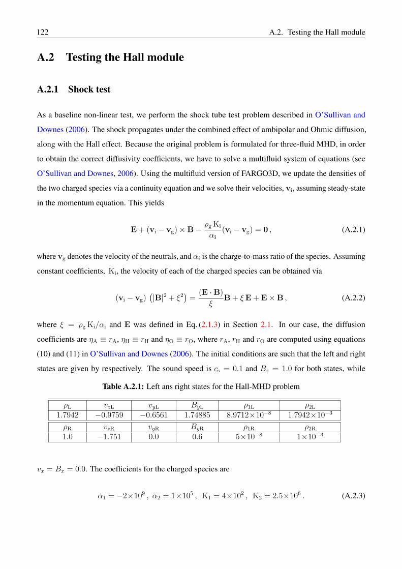
122 A.2. Testing the Hall module

A.2 Testing the Hall module

A.2.1 Shock test

As a baseline non-linear test, we perform the shock tube test problem described in O’Sullivan and

Downes (2006). The shock propagates under the combined effect of ambipolar and Ohmic diffusion,

along with the Hall effect. Because the original problem is formulated for three-fluid MHD, in order

to obtain the correct diffusivity coefficients, we have to solve a multifluid system of equations (see

O’Sullivan and Downes, 2006). Using the multifluid version of FARGO3D, we update the densities of

the two charged species via a continuity equation and we solve their velocities, vi, assuming steady-state

in the momentum equation. This yields

E + (vi − vg)×B− ρg Ki

αi

(vi − vg) = 0 , (A.2.1)

where vg denotes the velocity of the neutrals, and αi is the charge-to-mass ratio of the species. Assuming

constant coefficients, Ki, the velocity of each of the charged species can be obtained via

(vi − vg)(|B|2 + ξ2

)=

(E ·B)

ξB + ξE + E×B , (A.2.2)

where ξ = ρg Ki/αi and E was defined in Eq. (2.1.3) in Section 2.1. In our case, the diffusion

coefficients are ηA ≡ rA, ηH ≡ rH and ηO ≡ rO, where rA, rH and rO are computed using equations

(10) and (11) in O’Sullivan and Downes (2006). The initial conditions are such that the left and right

states are given by respectively. The sound speed is cs = 0.1 and Bz = 1.0 for both states, while

Table A.2.1: Left ans right states for the Hall-MHD problem

ρL vzL vyL ByL ρ1L ρ2L

1.7942 −0.9759 −0.6561 1.74885 8.9712×10−8 1.7942×10−3

ρR vzR vyR ByR ρ1R ρ2R

1.0 −1.751 0.0 0.6 5×10−8 1×10−3

vx = Bx = 0.0. The coefficients for the charged species are

α1 = −2×109 , α2 = 1×105 , K1 = 4×102 , K2 = 2.5×106 . (A.2.3)

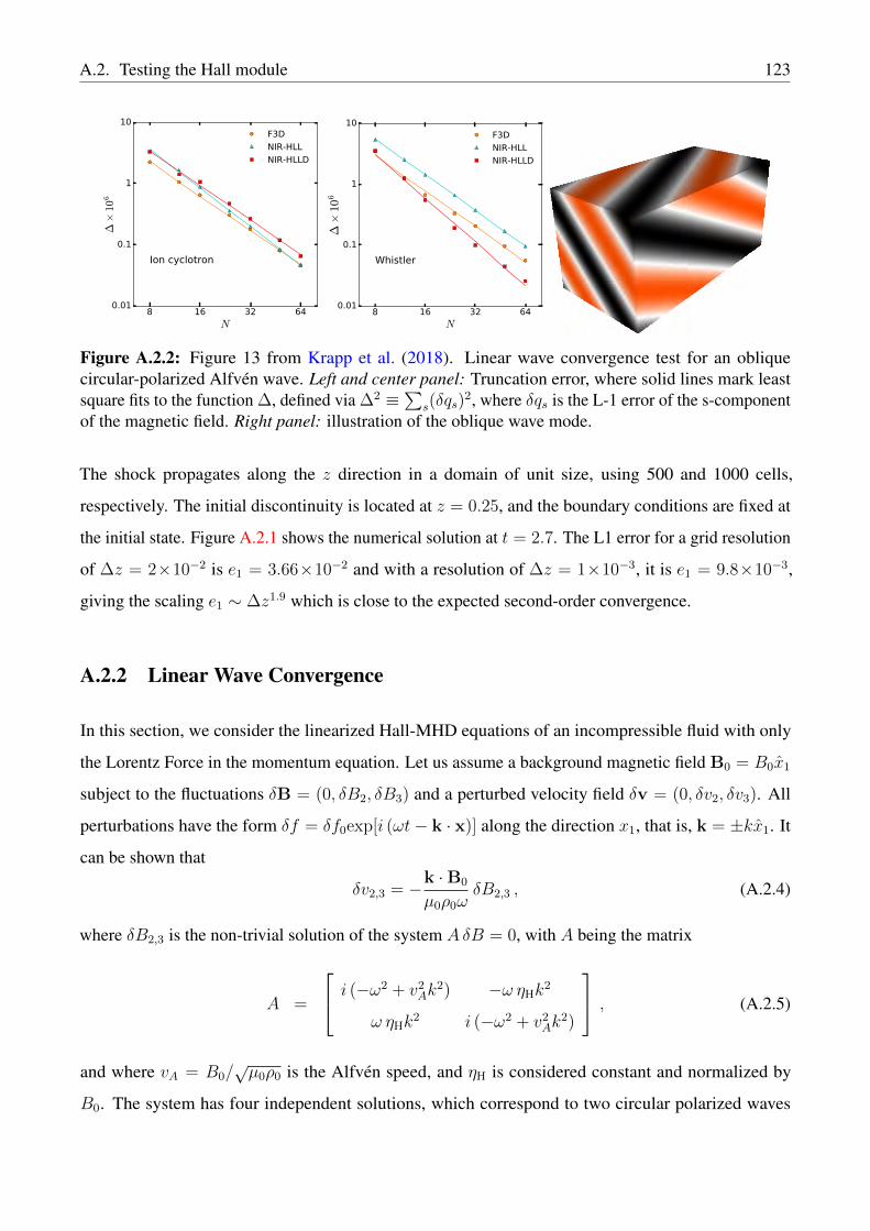
A.2. Testing the Hall module 123

8 16 32 64N

0.01

0.1

1

10

∆×

106

Ion cyclotron

F3D

NIR-HLL

NIR-HLLD

8 16 32 64N

0.01

0.1

1

10

∆×

10

6

Whistler

F3D

NIR-HLL

NIR-HLLD

Figure A.2.2: Figure 13 from Krapp et al. (2018). Linear wave convergence test for an obliquecircular-polarized Alfvén wave. Left and center panel: Truncation error, where solid lines mark leastsquare fits to the function ∆, defined via ∆2 ≡∑s(δqs)

2, where δqs is the L-1 error of the s-componentof the magnetic field. Right panel: illustration of the oblique wave mode.

The shock propagates along the z direction in a domain of unit size, using 500 and 1000 cells,

respectively. The initial discontinuity is located at z = 0.25, and the boundary conditions are fixed at

the initial state. Figure A.2.1 shows the numerical solution at t = 2.7. The L1 error for a grid resolution

of ∆z = 2×10−2 is e1 = 3.66×10−2 and with a resolution of ∆z = 1×10−3, it is e1 = 9.8×10−3,

giving the scaling e1 ∼ ∆z1.9 which is close to the expected second-order convergence.

A.2.2 Linear Wave Convergence

In this section, we consider the linearized Hall-MHD equations of an incompressible fluid with only

the Lorentz Force in the momentum equation. Let us assume a background magnetic field B0 = B0x1

subject to the fluctuations δB = (0, δB2, δB3) and a perturbed velocity field δv = (0, δv2, δv3). All

perturbations have the form δf = δf0exp[i (ωt− k · x)] along the direction x1, that is, k = ±kx1. It

can be shown that

δv2,3 = −k ·B0

µ0ρ0ωδB2,3 , (A.2.4)

where δB2,3 is the non-trivial solution of the system AδB = 0, with A being the matrix

A =

i (−ω2 + v2

Ak2) −ω ηHk

2

ω ηHk2 i (−ω2 + v2

Ak2)

, (A.2.5)

and where vA = B0/√µ0ρ0 is the Alfvén speed, and ηH is considered constant and normalized by

B0. The system has four independent solutions, which correspond to two circular polarized waves

124 A.2. Testing the Hall module

propagating along ±x1. For non-zero ηH, these waves are commonly know as the whistler mode and

the ion-cyclotron mode, respectively. Characteristically, these are dispersive waves, that is, the phase

velocity, ω/k, depends on the wavenumber. More precisely,

ω

k=ηH

2(k · eB)±

[1

4(kηH)2 + v2

A

] 12

, (A.2.6)

with eB the unit vector in the direction of B0.

In order test the newly developed Hall-MHD modules, we perform a convergence study of an oblique

wave propagation following a similar ansatz as the one presented in Gardiner and Stone (2008)

for circularly polarized waves in the ideal-MHD regime. We define a Cartesian periodic box with

dimensions (3, 1.5, 1.5), resolved by (2N,N,N) grid cells in x, y, and z, respectively. The propagation

is along the oblique coordinate x1 = kxx+ kyy + kzz, with

kx = 2π cos(α) cos(β) , ky = 2π cos(α) sin(β) , and kz = 2π cos(α) . (A.2.7)

We moreover set α = 2/3 and β = 2/√

5, in order to fit one wavelength λ = 1 inside the box.

The initial velocity field is ~v = (0, 10−6 cos(2πx1), 10−6 sin(2πx1)) and the initial magnetic field is

computed via a vector potential in such a way that B satisfies Eq. (A.2.4) with a background field

B0 = 1.0x1. The gas is treated as isothermal where P0 = c2sρ0, with an initial density ρ0 = 1.0 and gas

pressure P0 = 1.0. The Hall diffusion is set to ηH = 0.1.

We compute the L1-error for the centered components of the magnetic field as defined in Equation (70)

by Gardiner and Stone (2008), and we plot the results for different resolutions in Figure A.2.2. For

the Whistler mode NIRVANA-III returns an error e1 ∼ ∆2.3z and e1 ∼ ∆1.94

z , with the HLLD and HLL

solvers, respectively. This scaling is different for the Ion cyclotron mode, where e1 ∼ ∆1.87z with HLLD

solver and e1 ∼ ∆2.1z with the HLL scheme. In the case of FARGO3D, the error goes as e1 ∼ ∆z1.94

for the Whistler mode and e1 ∼ ∆z1.87 for the ion cyclotron mode. All the results are reasonably close

to the expected second order convergence of the implemented schemes.

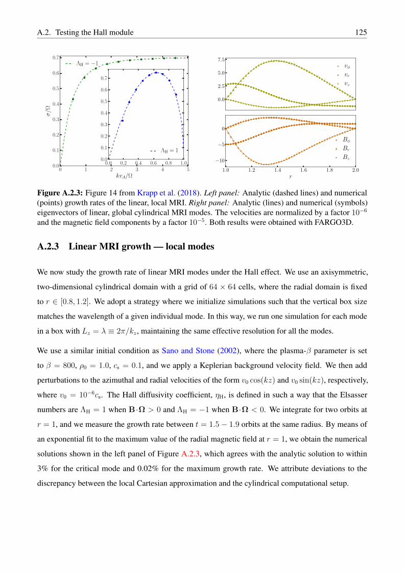
A.2. Testing the Hall module 125

0 1 2 3 4 5kvA/Ω

0.0

0.1

0.2

0.3

0.4

0.5

0.6

0.7

σ/Ω

ΛH = −1

0.0 0.2 0.4 0.6 0.8 1.00.0

0.1

0.2

0.3

0.4

0.5

0.6

0.7

ΛH = 1

0.0

2.5

5.0

7.5vφvrvz

1.0 1.2 1.4 1.6 1.8 2.0r

−10

−5

0

Bφ

Br

Bz

Figure A.2.3: Figure 14 from Krapp et al. (2018). Left panel: Analytic (dashed lines) and numerical(points) growth rates of the linear, local MRI. Right panel: Analytic (lines) and numerical (symbols)eigenvectors of linear, global cylindrical MRI modes. The velocities are normalized by a factor 10−6

and the magnetic field components by a factor 10−5. Both results were obtained with FARGO3D.

A.2.3 Linear MRI growth — local modes

We now study the growth rate of linear MRI modes under the Hall effect. We use an axisymmetric,

two-dimensional cylindrical domain with a grid of 64 × 64 cells, where the radial domain is fixed

to r ∈ [0.8, 1.2]. We adopt a strategy where we initialize simulations such that the vertical box size

matches the wavelength of a given individual mode. In this way, we run one simulation for each mode

in a box with Lz = λ ≡ 2π/kz, maintaining the same effective resolution for all the modes.

We use a similar initial condition as Sano and Stone (2002), where the plasma-β parameter is set

to β = 800, ρ0 = 1.0, cs = 0.1, and we apply a Keplerian background velocity field. We then add

perturbations to the azimuthal and radial velocities of the form v0 cos(kz) and v0 sin(kz), respectively,

where v0 = 10−6cs. The Hall diffusivity coefficient, ηH, is defined in such a way that the Elsasser

numbers are ΛH = 1 when B·Ω > 0 and ΛH = −1 when B·Ω < 0. We integrate for two orbits at

r = 1, and we measure the growth rate between t = 1.5− 1.9 orbits at the same radius. By means of

an exponential fit to the maximum value of the radial magnetic field at r = 1, we obtain the numerical

solutions shown in the left panel of Figure A.2.3, which agrees with the analytic solution to within

3% for the critical mode and 0.02% for the maximum growth rate. We attribute deviations to the

discrepancy between the local Cartesian approximation and the cylindrical computational setup.

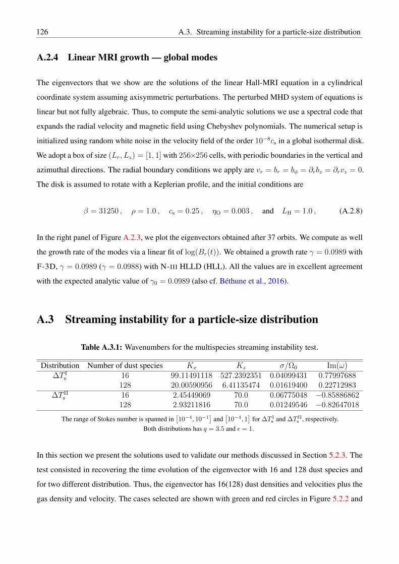
126 A.3. Streaming instability for a particle-size distribution

A.2.4 Linear MRI growth — global modes

The eigenvectors that we show are the solutions of the linear Hall-MRI equation in a cylindrical

coordinate system assuming axisymmetric perturbations. The perturbed MHD system of equations is

linear but not fully algebraic. Thus, to compute the semi-analytic solutions we use a spectral code that

expands the radial velocity and magnetic field using Chebyshev polynomials. The numerical setup is

initialized using random white noise in the velocity field of the order 10−8cs in a global isothermal disk.

We adopt a box of size (Lr, Lz) = [1, 1] with 256×256 cells, with periodic boundaries in the vertical and

azimuthal directions. The radial boundary conditions we apply are vr = br = bφ = ∂rbz = ∂rvz = 0.

The disk is assumed to rotate with a Keplerian profile, and the initial conditions are

β = 31250 , ρ = 1.0 , cs = 0.25 , ηO = 0.003 , and LH = 1.0 , (A.2.8)

In the right panel of Figure A.2.3, we plot the eigenvectors obtained after 37 orbits. We compute as well

the growth rate of the modes via a linear fit of log(Br(t)). We obtained a growth rate γ = 0.0989 with

F-3D, γ = 0.0989 (γ = 0.0988) with N-III HLLD (HLL). All the values are in excellent agreement

with the expected analytic value of γ0 = 0.0989 (also cf. Béthune et al., 2016).

A.3 Streaming instability for a particle-size distribution

Table A.3.1: Wavenumbers for the multispecies streaming instability test.

Distribution Number of dust species Kx Kz σ/Ω0 Im(ω)∆T I

s 16 99.11491118 527.2392351 0.04099431 0.77997688128 20.00590956 6.41135474 0.01619400 0.22712983

∆T IIs 16 2.45449069 70.0 0.06775048 −0.85886862

128 2.93211816 70.0 0.01249546 −0.82647018

The range of Stokes number is spanned in[10−4, 10−1

]and

[10−4, 1

]for ∆T I

s and ∆T IIs , respectively.

Both distributions has q = 3.5 and ε = 1.

In this section we present the solutions used to validate our methods discussed in Section 5.2.3. The

test consisted in recovering the time evolution of the eigenvector with 16 and 128 dust species and

for two different distribution. Thus, the eigenvector has 16(128) dust densities and velocities plus the

gas density and velocity. The cases selected are shown with green and red circles in Figure 5.2.2 and

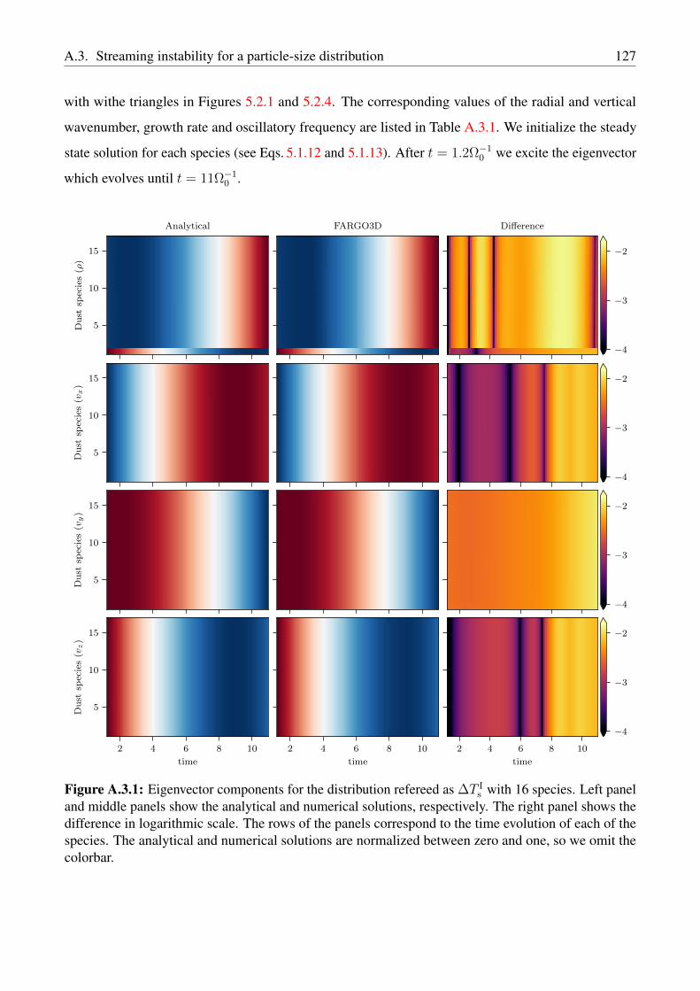
A.3. Streaming instability for a particle-size distribution 127

with withe triangles in Figures 5.2.1 and 5.2.4. The corresponding values of the radial and vertical

wavenumber, growth rate and oscillatory frequency are listed in Table A.3.1. We initialize the steady

state solution for each species (see Eqs. 5.1.12 and 5.1.13). After t = 1.2Ω−10 we excite the eigenvector

which evolves until t = 11Ω−10 .

5

10

15

Du

stsp

ecie

s(ρ

)

Analytical FARGO3D Difference

5

10

15

Du

stsp

ecie

s(vx)

5

10

15

Du

stsp

ecie

s(vy)

2 4 6 8 10

time

5

10

15

Du

stsp

ecie

s(vz)

2 4 6 8 10

time

2 4 6 8 10

time

−4

−3

−2

−4

−3

−2

−4

−3

−2

−4

−3

−2

Figure A.3.1: Eigenvector components for the distribution refereed as ∆T Is with 16 species. Left panel

and middle panels show the analytical and numerical solutions, respectively. The right panel shows thedifference in logarithmic scale. The rows of the panels correspond to the time evolution of each of thespecies. The analytical and numerical solutions are normalized between zero and one, so we omit thecolorbar.

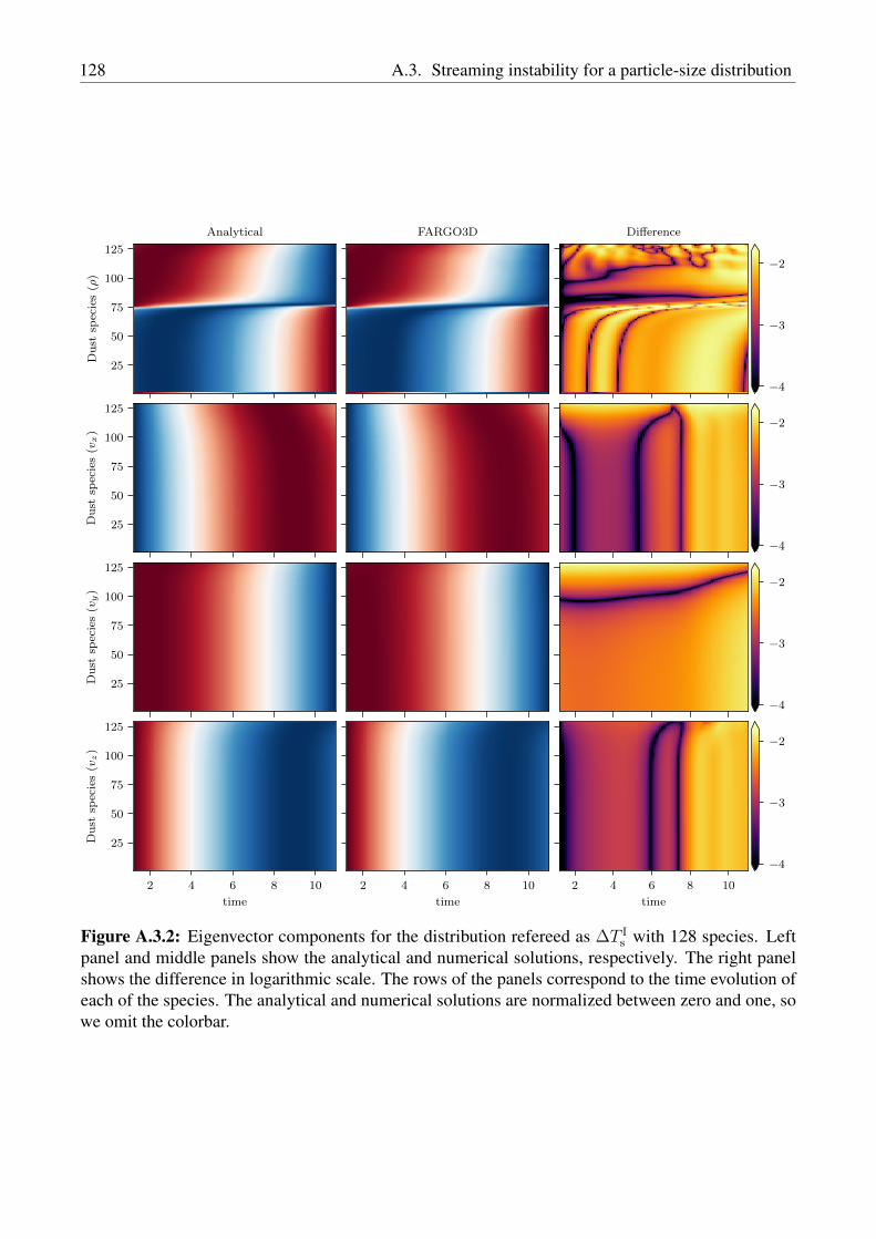
128 A.3. Streaming instability for a particle-size distribution

25

50

75

100

125

Du

stsp

ecie

s(ρ

)

Analytical FARGO3D Difference

25

50

75

100

125

Du

stsp

ecie

s(vx)

25

50

75

100

125

Du

stsp

ecie

s(vy)

2 4 6 8 10

time

25

50

75

100

125

Du

stsp

ecie

s(vz)

2 4 6 8 10

time

2 4 6 8 10

time

−4

−3

−2

−4

−3

−2

−4

−3

−2

−4

−3

−2

Figure A.3.2: Eigenvector components for the distribution refereed as ∆T Is with 128 species. Left

panel and middle panels show the analytical and numerical solutions, respectively. The right panelshows the difference in logarithmic scale. The rows of the panels correspond to the time evolution ofeach of the species. The analytical and numerical solutions are normalized between zero and one, sowe omit the colorbar.

A.3. Streaming instability for a particle-size distribution 129

5

10

15

Du

stsp

ecie

s(ρ

)

Analytical FARGO3D Difference

5

10

15

Du

stsp

ecie

s(vx)

5

10

15

Du

stsp

ecie

s(vy)

2 4 6 8 10

time

5

10

15

Du

stsp

ecie

s(vz)

2 4 6 8 10

time

2 4 6 8 10

time

−4

−3

−2

−4

−3

−2

−4

−3

−2

−4

−3

−2

Figure A.3.3: Eigenvector components for the distribution refereed as ∆T IIs with 16 species. Left panel

and middle panels show the analytical and numerical solutions, respectively. The right panel shows thedifference in logarithmic scale. The rows of the panels correspond to the time evolution of each of thespecies. The analytical and numerical solutions are normalized between zero and one, so we omit thecolorbar.

130 A.3. Streaming instability for a particle-size distribution

25

50

75

100

125

Du

stsp

ecie

s(ρ

)

Analytical FARGO3D Difference

25

50

75

100

125

Du

stsp

ecie

s(vx)

25

50

75

100

125

Du

stsp

ecie

s(vy)

2 4 6 8 10

time

25

50

75

100

125

Du

stsp

ecie

s(vz)

2 4 6 8 10

time

2 4 6 8 10

time

−4

−3

−2

−4

−3

−2

−4

−3

−2

−4

−3

−2

Figure A.3.4: Eigenvector components for the distribution refereed as ∆T IIs with 128 species. Left

panel and middle panels show the analytical and numerical solutions, respectively. The right panelshows the difference in logarithmic scale. The rows of the panels correspond to the time evolution ofeach of the species. The analytical and numerical solutions are normalized between zero and one, sowe omit the colorbar.

Bibliography

Alexander, R., Pascucci, I., Andrews, S., Armitage, P., and Cieza, L. (2014). The Dispersal of

Protoplanetary Disks. Protostars and Planets VI, pages 475–496.

Alexander, R. D., Clarke, C. J., and Pringle, J. E. (2006). Photoevaporation of protoplanetary discs - II.

Evolutionary models and observable properties. MNRAS, 369(1):229–239.

Alexiades, V., Amiez, G., and Gremaud, P.-A. (1996). Super-time-stepping acceleration of explicit

schemes for parabolic problems. Comm. in Num. Methods in Engineering, 12(1):31–42.

ALMA Partnership, Brogan, C. L., Pérez, L. M., Hunter, T. R., Dent, W. R. F., Hales, A. S., Hills,

R. E., Corder, S., Fomalont, E. B., and Vlahakis, C. (2015). The 2014 ALMA Long Baseline

Campaign: First Results from High Angular Resolution Observations toward the HL Tau Region.

ApJ, 808(1):L3.

Anderson, E., Bai, Z., Bischof, C., Blackford, S., Demmel, J., Dongarra, J., Du Croz, J., Greenbaum,

A., Hammarling, S., McKenney, A., and Sorensen, D. (1999). LAPACK Users’ Guide. Society for

Industrial and Applied Mathematics, Philadelphia, PA, third edition.

Andrews, S. M., Huang, J., Pérez, L. M., Isella, A., Dullemond, C. P., Kurtovic, N. T., Guzmán, V. V.,

Carpenter, J. M., Wilner, D. J., and Zhang, S. (2018). The Disk Substructures at High Angular

Resolution Project (DSHARP). I. Motivation, Sample, Calibration, and Overview. ApJ, 869(2):L41.

Andrews, S. M., Wilner, D. J., Zhu, Z., Birnstiel, T., Carpenter, J. M., Pérez, L. M., Bai, X.-N., Öberg,

K. I., Hughes, A. M., Isella, A., and Ricci, L. (2016). RINGED SUBSTRUCTURE AND a GAP AT

1 au IN THE NEAREST PROTOPLANETARY DISK. The Astrophysical Journal, 820(2):L40.

131

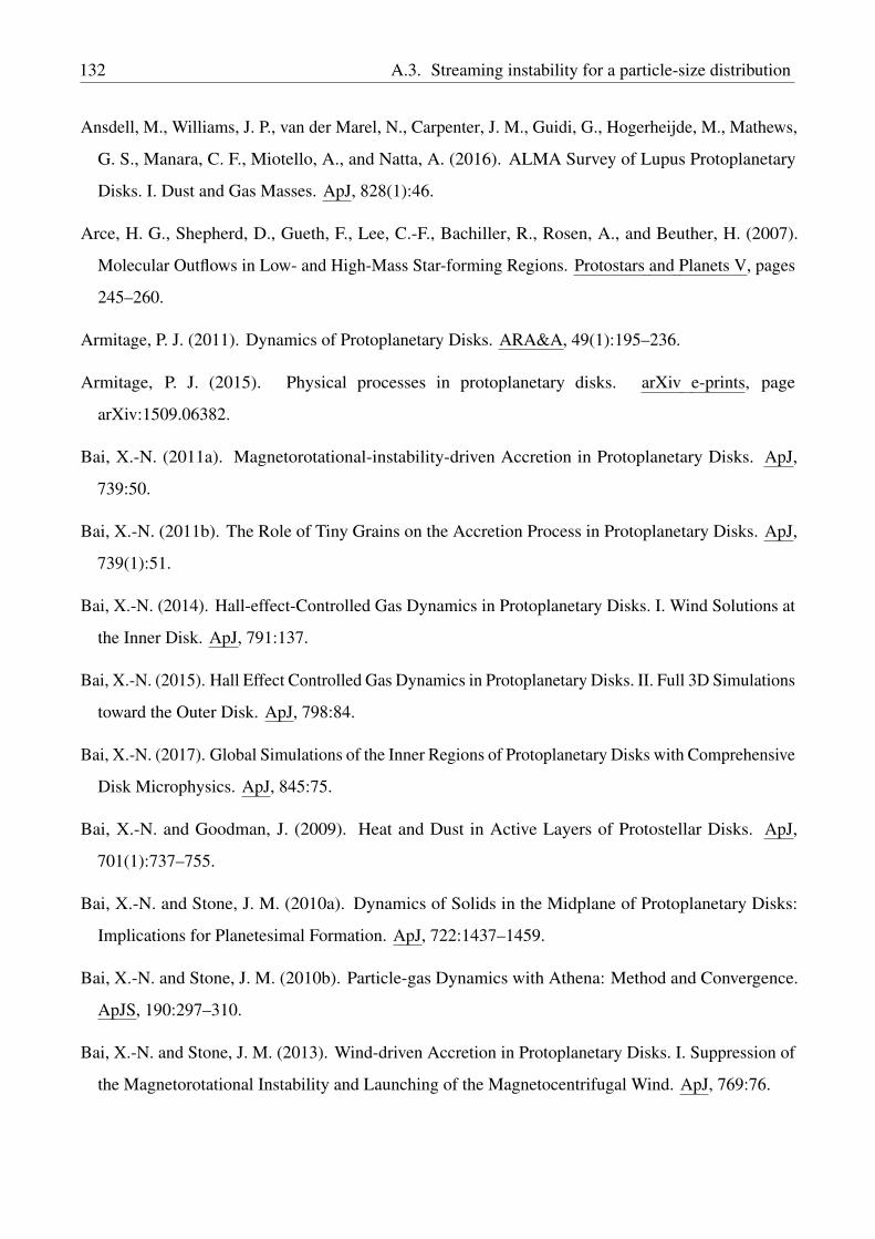
132 A.3. Streaming instability for a particle-size distribution

Ansdell, M., Williams, J. P., van der Marel, N., Carpenter, J. M., Guidi, G., Hogerheijde, M., Mathews,

G. S., Manara, C. F., Miotello, A., and Natta, A. (2016). ALMA Survey of Lupus Protoplanetary

Disks. I. Dust and Gas Masses. ApJ, 828(1):46.

Arce, H. G., Shepherd, D., Gueth, F., Lee, C.-F., Bachiller, R., Rosen, A., and Beuther, H. (2007).

Molecular Outflows in Low- and High-Mass Star-forming Regions. Protostars and Planets V, pages

245–260.

Armitage, P. J. (2011). Dynamics of Protoplanetary Disks. ARA&A, 49(1):195–236.

Armitage, P. J. (2015). Physical processes in protoplanetary disks. arXiv e-prints, page

arXiv:1509.06382.

Bai, X.-N. (2011a). Magnetorotational-instability-driven Accretion in Protoplanetary Disks. ApJ,

739:50.

Bai, X.-N. (2011b). The Role of Tiny Grains on the Accretion Process in Protoplanetary Disks. ApJ,

739(1):51.

Bai, X.-N. (2014). Hall-effect-Controlled Gas Dynamics in Protoplanetary Disks. I. Wind Solutions at

the Inner Disk. ApJ, 791:137.

Bai, X.-N. (2015). Hall Effect Controlled Gas Dynamics in Protoplanetary Disks. II. Full 3D Simulations

toward the Outer Disk. ApJ, 798:84.

Bai, X.-N. (2017). Global Simulations of the Inner Regions of Protoplanetary Disks with Comprehensive

Disk Microphysics. ApJ, 845:75.

Bai, X.-N. and Goodman, J. (2009). Heat and Dust in Active Layers of Protostellar Disks. ApJ,

701(1):737–755.

Bai, X.-N. and Stone, J. M. (2010a). Dynamics of Solids in the Midplane of Protoplanetary Disks:

Implications for Planetesimal Formation. ApJ, 722:1437–1459.

Bai, X.-N. and Stone, J. M. (2010b). Particle-gas Dynamics with Athena: Method and Convergence.

ApJS, 190:297–310.

Bai, X.-N. and Stone, J. M. (2013). Wind-driven Accretion in Protoplanetary Disks. I. Suppression of

the Magnetorotational Instability and Launching of the Magnetocentrifugal Wind. ApJ, 769:76.

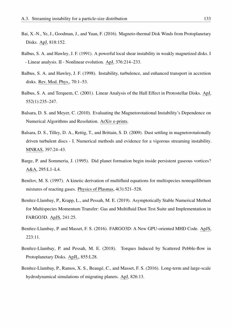
A.3. Streaming instability for a particle-size distribution 133

Bai, X.-N., Ye, J., Goodman, J., and Yuan, F. (2016). Magneto-thermal Disk Winds from Protoplanetary

Disks. ApJ, 818:152.

Balbus, S. A. and Hawley, J. F. (1991). A powerful local shear instability in weakly magnetized disks. I

- Linear analysis. II - Nonlinear evolution. ApJ, 376:214–233.

Balbus, S. A. and Hawley, J. F. (1998). Instability, turbulence, and enhanced transport in accretion

disks. Rev. Mod. Phys., 70:1–53.

Balbus, S. A. and Terquem, C. (2001). Linear Analysis of the Hall Effect in Protostellar Disks. ApJ,

552(1):235–247.

Balsara, D. S. and Meyer, C. (2010). Evaluating the Magnetorotational Instability’s Dependence on

Numerical Algorithms and Resolution. ArXiv e-prints.

Balsara, D. S., Tilley, D. A., Rettig, T., and Brittain, S. D. (2009). Dust settling in magnetorotationally

driven turbulent discs - I. Numerical methods and evidence for a vigorous streaming instability.

MNRAS, 397:24–43.

Barge, P. and Sommeria, J. (1995). Did planet formation begin inside persistent gaseous vortices?

A&A, 295:L1–L4.

Benilov, M. S. (1997). A kinetic derivation of multifluid equations for multispecies nonequilibrium

mixtures of reacting gases. Physics of Plasmas, 4(3):521–528.

Benítez-Llambay, P., Krapp, L., and Pessah, M. E. (2019). Asymptotically Stable Numerical Method

for Multispecies Momentum Transfer: Gas and Multifluid Dust Test Suite and Implementation in

FARGO3D. ApJS, 241:25.

Benítez-Llambay, P. and Masset, F. S. (2016). FARGO3D: A New GPU-oriented MHD Code. ApJS,

223:11.

Benítez-Llambay, P. and Pessah, M. E. (2018). Torques Induced by Scattered Pebble-flow in

Protoplanetary Disks. ApJL, 855:L28.

Benítez-Llambay, P., Ramos, X. S., Beaugé, C., and Masset, F. S. (2016). Long-term and large-scale

hydrodynamical simulations of migrating planets. ApJ, 826:13.

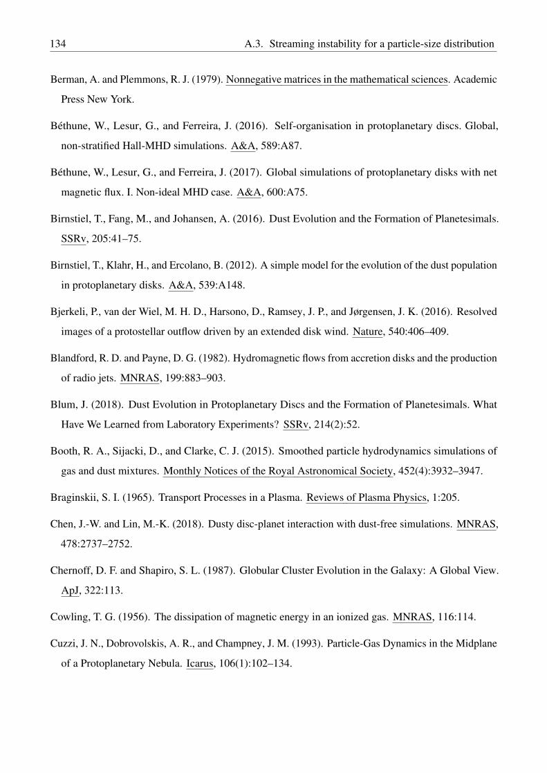
134 A.3. Streaming instability for a particle-size distribution

Berman, A. and Plemmons, R. J. (1979). Nonnegative matrices in the mathematical sciences. Academic

Press New York.

Béthune, W., Lesur, G., and Ferreira, J. (2016). Self-organisation in protoplanetary discs. Global,

non-stratified Hall-MHD simulations. A&A, 589:A87.

Béthune, W., Lesur, G., and Ferreira, J. (2017). Global simulations of protoplanetary disks with net

magnetic flux. I. Non-ideal MHD case. A&A, 600:A75.

Birnstiel, T., Fang, M., and Johansen, A. (2016). Dust Evolution and the Formation of Planetesimals.

SSRv, 205:41–75.

Birnstiel, T., Klahr, H., and Ercolano, B. (2012). A simple model for the evolution of the dust population

in protoplanetary disks. A&A, 539:A148.

Bjerkeli, P., van der Wiel, M. H. D., Harsono, D., Ramsey, J. P., and Jørgensen, J. K. (2016). Resolved

images of a protostellar outflow driven by an extended disk wind. Nature, 540:406–409.

Blandford, R. D. and Payne, D. G. (1982). Hydromagnetic flows from accretion disks and the production

of radio jets. MNRAS, 199:883–903.

Blum, J. (2018). Dust Evolution in Protoplanetary Discs and the Formation of Planetesimals. What

Have We Learned from Laboratory Experiments? SSRv, 214(2):52.

Booth, R. A., Sijacki, D., and Clarke, C. J. (2015). Smoothed particle hydrodynamics simulations of

gas and dust mixtures. Monthly Notices of the Royal Astronomical Society, 452(4):3932–3947.

Braginskii, S. I. (1965). Transport Processes in a Plasma. Reviews of Plasma Physics, 1:205.

Chen, J.-W. and Lin, M.-K. (2018). Dusty disc-planet interaction with dust-free simulations. MNRAS,

478:2737–2752.

Chernoff, D. F. and Shapiro, S. L. (1987). Globular Cluster Evolution in the Galaxy: A Global View.

ApJ, 322:113.

Cowling, T. G. (1956). The dissipation of magnetic energy in an ionized gas. MNRAS, 116:114.

Cuzzi, J. N., Dobrovolskis, A. R., and Champney, J. M. (1993). Particle-Gas Dynamics in the Midplane

of a Protoplanetary Nebula. Icarus, 106(1):102–134.

A.3. Streaming instability for a particle-size distribution 135

de Val-Borro, M., Edgar, R., Artymowicz, P., Ciecielag, P., Cresswell, P., D’Angelo, G., Delgado-

Donate, E., Dirksen, G., Fromang, S., Gawryszczak, A., Klahr, H., Kley, W., Lyra, W., Masset, F.,

Mellema, G., Nelson, R., Paardekooper, S.-J., Peplinski, A., Pierens, A., Plewa, T., Rice, K., Schäfer,

C., and Speith, R. (2006). A comparative study of disc-planet interaction. MNRAS, 370:529–558.

de Val-Borro, M., Edgar, R. G., Artymowicz, P., Ciecielag, P., Cresswell, P., D’Angelo, G., Delgado-

Donate, E. J., Dirksen, G., Fromang, S., Gawryszczak, A., Klahr, H., Kley, W., Lyra, W., Masset,

F., Mellema, G., Nelson, R. P., Paardekooper, S.-J., Peplinski, A., Pierens, A., Plewa, T., Rice,

K., Schäfer, C., and Speith, R. (2006). A comparative study of disc-planet interaction. MNRAS,

370:529–558.

Dipierro, G., Laibe, G., Alexander, R., and Hutchison, M. (2018). Gas and multispecies dust dynamics

in viscous protoplanetary discs: the importance of the dust back-reaction. MNRAS, 479:4187–4206.

Dittrich, K., Klahr, H., and Johansen, A. (2013). Gravoturbulent Planetesimal Formation: The Positive

Effect of Long-lived Zonal Flows. ApJ, 763:117.

Dohnanyi, J. S. (1969). Collisional Model of Asteroids and Their Debris. J. Geophys. Res., 74:2531–

2554.

Draine, B. T. (1986). Multicomponent, reacting MHD flows. MNRAS, 220:133–148.

Draine, B. T. and Salpeter, E. E. (1979). On the physics of dust grains in hot gas. ApJ, 231:77–94.

Epstein, P. S. (1924). On the resistance experienced by spheres in their motion through gases. Phys.

Rev., 23:710–733.

Ercolano, B. and Glassgold, A. E. (2013). X-ray ionization rates in protoplanetary discs. Monthly

Notices of the Royal Astronomical Society, 436(4):3446–3450.

Evans, C. R. and Hawley, J. F. (1988). Simulation of magnetohydrodynamic flows - A constrained

transport method. ApJ, 332:659–677.

Falle, S. A. E. G. (2003). A numerical scheme for multifluid magnetohydrodynamics. MNRAS,

344(4):1210–1218.

Flock, M., Dzyurkevich, N., Klahr, H., and Mignone, A. (2010). High-order Godunov schemes for

global 3D MHD simulations of accretion disks. I. Testing the linear growth of the magneto-rotational

instability. A&A, 516:A26.

136 A.3. Streaming instability for a particle-size distribution

Flock, M., Dzyurkevich, N., Klahr, H., Turner, N. J., and Henning, T. (2011). Turbulence and Steady

Flows in Three-dimensional Global Stratified Magnetohydrodynamic Simulations of Accretion Disks.

ApJ, 735(2):122.

Fromang, S., Terquem, C., and Balbus, S. A. (2002). The ionization fraction in α models of

protoplanetary discs. MNRAS, 329:18–28.

Garaud, P., Barrière-Fouchet, L., and Lin, D. N. C. (2004). Individual and Average Behavior of Particles

in a Protoplanetary Nebula. ApJ, 603:292–306.

Gardiner, T. A. and Stone, J. M. (2008). An unsplit Godunov method for ideal MHD via constrained

transport in three dimensions. Journal of Computational Physics, 227:4123–4141.

Geršgorin, S. (1931). Über die Abgrenzung der Eigenwerte einer Matrix. Bulletin de l’Académie des

Sciences de l’URSS. Classe des sciences mathématiques et na, 6:749–754.

Gressel, O., Turner, N. J., Nelson, R. P., and McNally, C. P. (2015). Global Simulations of Protoplanetary

Disks With Ohmic Resistivity and Ambipolar Diffusion. ApJ, 801:84.

Hartmann, L., Calvet, N., Gullbring, E., and D'Alessio, P. (1998). Accretion and the evolution of t tauri

disks. The Astrophysical Journal, 495(1):385–400.

Hawley, J. F., Gammie, C. F., and Balbus, S. A. (1995). Local Three-dimensional

Magnetohydrodynamic Simulations of Accretion Disks. ApJ, 440:742.

Hayashi, C. (1981). Structure of the solar nebula, growth and decay of magnetic fields and effects

of magnetic and turbulent viscosities on the nebula. Progress of Theoretical Physics Supplement,

70:35–53.

Huba, J. D. (2003). Hall Magnetohydrodynamics - A Tutorial. In Büchner, J., Dum, C., and Scholer, M.,

editors, Space Plasma Simulation, volume 615 of Lecture Notes in Physics, Berlin Springer Verlag,

pages 166–192.

Igea, J. and Glassgold, A. E. (1999). X-Ray Ionization of the Disks of Young Stellar Objects. ApJ,

518:848–858.

Ilgner, M. and Nelson, R. P. (2006). On the ionisation fraction in protoplanetary disks. I. Comparing

different reaction networks. A&A, 445:205–222.

A.3. Streaming instability for a particle-size distribution 137

Johansen, A. and Youdin, A. (2007). Protoplanetary Disk Turbulence Driven by the Streaming

Instability: Nonlinear Saturation and Particle Concentration. ApJ, 662:627–641.

Johansen, A. and Youdin, A. (2007). Protoplanetary disk turbulence driven by the streaming instability:

Nonlinear saturation and particle concentration. The Astrophysical Journal, 662(1):627.

Johansen, A., Youdin, A., and Klahr, H. (2009). Zonal Flows and Long-lived Axisymmetric Pressure

Bumps in Magnetorotational Turbulence. ApJ, 697:1269–1289.

Keith, S. L. and Wardle, M. (2015). Magnetic fields in gaps surrounding giant protoplanets. MNRAS,

451:1104–1116.

Klahr, H. and Hubbard, A. (2014). CONVECTIVE OVERSTABILITY IN RADIALLY STRATIFIED

ACCRETION DISKS UNDER THERMAL RELAXATION. The Astrophysical Journal, 788(1):21.

Klahr, H. H. and Henning, T. (1997). Particle-Trapping Eddies in Protoplanetary Accretion Disks.

Icarus, 128:213–229.

Kounkel, M., Hartmann, L., Loinard, L., Ortiz-León, G. N., Mioduszewski, A. J., Rodríguez, L. F., Dzib,

S. A., Torres, R. M., Pech, G., Galli, P. A. B., Rivera, J. L., Boden, A. F., II, N. J. E., Briceño, C., and

Tobin, J. J. (2017). THE GOULD’s BELT DISTANCES SURVEY (GOBELINS). II. DISTANCES

AND STRUCTURE TOWARD THE ORION MOLECULAR CLOUDS. The Astrophysical Journal,

834(2):142.

Kowalik, K., Hanasz, M., Wóltanski, D., and Gawryszczak, A. (2013). Streaming instability in the

quasi-global protoplanetary discs. MNRAS, 434:1460–1468.

Krapp, L., Benítez-Llambay, P., Gressel, O., and Pessah, M. E. (2019). Streaming Instability for

Particle-size Distributions. ApJ, 878(2):L30.

Krapp, L., Gressel, O., Benítez-Llambay, P., Downes, T. P., Mohandas, G., and Pessah, M. E. (2018).

Dust Segregation in Hall-dominated Turbulent Protoplanetary Disks. ApJ, 865:105.

Kunz, M. W. and Lesur, G. (2013). Magnetic self-organization in Hall-dominated magnetorotational

turbulence. MNRAS, 434:2295–2312.

Laibe, G. and Price, D. J. (2012). Dusty gas with smoothed particle hydrodynamics - I. Algorithm and

test suite. MNRAS, 420:2345–2364.

138 A.3. Streaming instability for a particle-size distribution

Laibe, G. and Price, D. J. (2014). Dusty gas with one fluid. MNRAS, 440:2136–2146.

Lesur, G., Kunz, M. W., and Fromang, S. (2014). Thanatology in protoplanetary discs. The combined

influence of Ohmic, Hall, and ambipolar diffusion on dead zones. A&A, 566:A56.

Lesur, G. and Papaloizou, J. C. B. (2010). The subcritical baroclinic instability in local accretion disc

models. A&A, 513:A60.

Lin, M.-K. (2019). Dust settling against hydrodynamic turbulence in protoplanetary discs. MNRAS,

485:5221–5234.

Lin, M.-K. and Youdin, A. N. (2017). A Thermodynamic View of Dusty Protoplanetary Disks. ApJ,

849:129.

Lissauer, J. J. (1993). Planet formation. ARA&A, 31:129–174.

Londrillo, P. and del Zanna, L. (2004). On the divergence-free condition in Godunov-type schemes for

ideal magnetohydrodynamics: the upwind constrained transport method. Journal of Computational

Physics, 195:17–48.

Lynden-Bell, D. (1996). Magnetic collimation by accretion discs of quasars and stars. MNRAS,

279:389–401.

Lynden-Bell, D. and Pringle, J. E. (1974). The evolution of viscous discs and the origin of the nebular

variables. MNRAS, 168:603–637.

Marcus, P. S., Pei, S., Jiang, C.-H., Barranco, J. A., Hassanzadeh, P., and Lecoanet, D. (2015). ZOMBIE

VORTEX INSTABILITY. i. a PURELY HYDRODYNAMIC INSTABILITY TO RESURRECT

THE DEAD ZONES OF PROTOPLANETARY DISKS. The Astrophysical Journal, 808(1):87.

Masset, F. (2000). FARGO: A fast eulerian transport algorithm for differentially rotating disks. A&AS,

141:165–173.

Mathis, J. S., Rumpl, W., and Nordsieck, K. H. (1977). The size distribution of interstellar grains. ApJ,

217:425–433.

Mayor, M. and Queloz, D. (1995). A Jupiter-mass companion to a solar-type star. Nature, 378:355–359.

McCall, B. J., Huneycutt, A. J., Saykally, R. J., Geballe, T. R., Djuric, N., Dunn, G. H., Semaniak, J.,

Novotny, O., Al-Khalili, A., Ehlerding, A., Hellberg, F., Kalhori, S., Neau, A., Thomas, R., Österdahl,

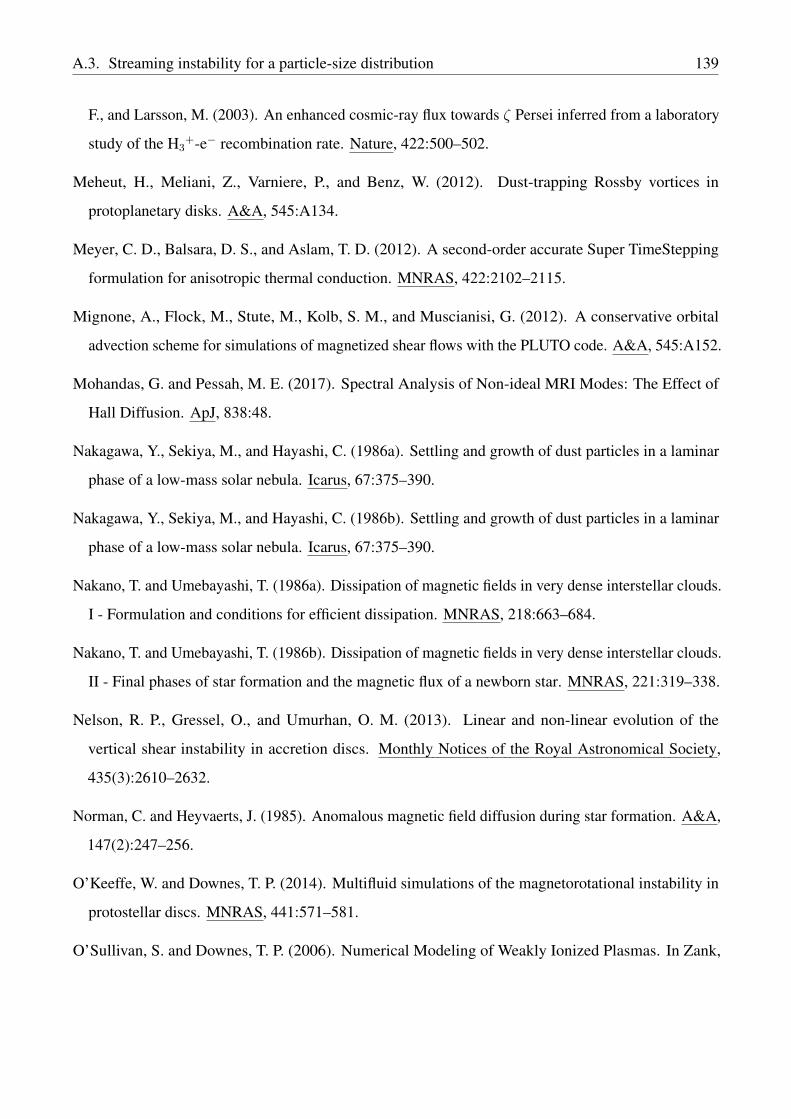
A.3. Streaming instability for a particle-size distribution 139

F., and Larsson, M. (2003). An enhanced cosmic-ray flux towards ζ Persei inferred from a laboratory

study of the H3+-e− recombination rate. Nature, 422:500–502.

Meheut, H., Meliani, Z., Varniere, P., and Benz, W. (2012). Dust-trapping Rossby vortices in

protoplanetary disks. A&A, 545:A134.

Meyer, C. D., Balsara, D. S., and Aslam, T. D. (2012). A second-order accurate Super TimeStepping

formulation for anisotropic thermal conduction. MNRAS, 422:2102–2115.

Mignone, A., Flock, M., Stute, M., Kolb, S. M., and Muscianisi, G. (2012). A conservative orbital

advection scheme for simulations of magnetized shear flows with the PLUTO code. A&A, 545:A152.

Mohandas, G. and Pessah, M. E. (2017). Spectral Analysis of Non-ideal MRI Modes: The Effect of

Hall Diffusion. ApJ, 838:48.

Nakagawa, Y., Sekiya, M., and Hayashi, C. (1986a). Settling and growth of dust particles in a laminar

phase of a low-mass solar nebula. Icarus, 67:375–390.

Nakagawa, Y., Sekiya, M., and Hayashi, C. (1986b). Settling and growth of dust particles in a laminar

phase of a low-mass solar nebula. Icarus, 67:375–390.

Nakano, T. and Umebayashi, T. (1986a). Dissipation of magnetic fields in very dense interstellar clouds.

I - Formulation and conditions for efficient dissipation. MNRAS, 218:663–684.

Nakano, T. and Umebayashi, T. (1986b). Dissipation of magnetic fields in very dense interstellar clouds.

II - Final phases of star formation and the magnetic flux of a newborn star. MNRAS, 221:319–338.

Nelson, R. P., Gressel, O., and Umurhan, O. M. (2013). Linear and non-linear evolution of the

vertical shear instability in accretion discs. Monthly Notices of the Royal Astronomical Society,

435(3):2610–2632.

Norman, C. and Heyvaerts, J. (1985). Anomalous magnetic field diffusion during star formation. A&A,

147(2):247–256.

O’Keeffe, W. and Downes, T. P. (2014). Multifluid simulations of the magnetorotational instability in

protostellar discs. MNRAS, 441:571–581.

O’Sullivan, S. and Downes, T. P. (2006). Numerical Modeling of Weakly Ionized Plasmas. In Zank,

140 A.3. Streaming instability for a particle-size distribution

G. P. and Pogorelov, N. V., editors, Numerical Modeling of Space Plasma Flows, volume 359 of

Astronomical Society of the Pacific Conference Series, page 178.

O’Sullivan, S. and Downes, T. P. (2007). A three-dimensional numerical method for modelling weakly

ionized plasmas. MNRAS, 376:1648–1658.

Pandey, B. P. and Wardle, M. (2008). Hall magnetohydrodynamics of partially ionized plasmas.

MNRAS, 385:2269–2278.

Perez-Becker, D. and Chiang, E. (2011). SURFACE LAYER ACCRETION IN CONVENTIONAL

AND TRANSITIONAL DISKS DRIVEN BY FAR-ULTRAVIOLET IONIZATION. The

Astrophysical Journal, 735(1):8.

Perron, O. (1907). Zur theorie der matrices. Mathematische Annalen, 64:248–263.

Pinilla, P., Birnstiel, T., Ricci, L., Dullemond, C. P., Uribe, A. L., Testi, L., and Natta, A. (2012).

Trapping dust particles in the outer regions of protoplanetary disks. A&A, 538:A114.

Pinte, C., Dent, W. R. F., Ménard, F., Hales, A., Hill, T., Cortes, P., and de Gregorio-Monsalvo, I. (2016).

Dust and Gas in the Disk of HL Tauri: Surface Density, Dust Settling, and Dust-to-gas Ratio. ApJ,

816:25.

Polygiannakis, J. M. and Moussas, X. (2001). A review of magneto-vorticity induction in hall-mhd

plasmas. Plasma Physics and Controlled Fusion, 43(2):195.

Press, W. H., Teukolsky, S. A., Vetterling, W. T., and Flannery, B. P. (2007). Numerical Recipes 3rd

Edition: The Art of Scientific Computing. Cambridge University Press, New York, NY, USA, 3

edition.

Raettig, N., Klahr, H., and Lyra, W. (2015). Particle Trapping and Streaming Instability in Vortices in

Protoplanetary Disks. ApJ, 804:35.

Ragusa, E., Dipierro, G., Lodato, G., Laibe, G., and Price, D. J. (2017). On the origin of horseshoes in

transitional discs. MNRAS, 464:1449–1455.

Riols, A. and Lesur, G. (2018). Dust settling and rings in the outer regions of protoplanetary discs

subject to ambipolar diffusion. A&A, 617:A117.

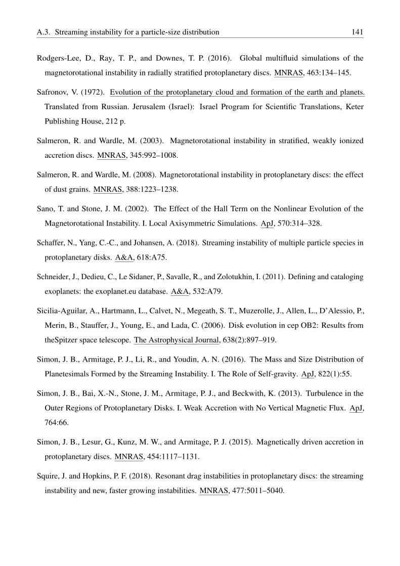
A.3. Streaming instability for a particle-size distribution 141

Rodgers-Lee, D., Ray, T. P., and Downes, T. P. (2016). Global multifluid simulations of the

magnetorotational instability in radially stratified protoplanetary discs. MNRAS, 463:134–145.

Safronov, V. (1972). Evolution of the protoplanetary cloud and formation of the earth and planets.

Translated from Russian. Jerusalem (Israel): Israel Program for Scientific Translations, Keter

Publishing House, 212 p.

Salmeron, R. and Wardle, M. (2003). Magnetorotational instability in stratified, weakly ionized

accretion discs. MNRAS, 345:992–1008.

Salmeron, R. and Wardle, M. (2008). Magnetorotational instability in protoplanetary discs: the effect

of dust grains. MNRAS, 388:1223–1238.

Sano, T. and Stone, J. M. (2002). The Effect of the Hall Term on the Nonlinear Evolution of the

Magnetorotational Instability. I. Local Axisymmetric Simulations. ApJ, 570:314–328.

Schaffer, N., Yang, C.-C., and Johansen, A. (2018). Streaming instability of multiple particle species in

protoplanetary disks. A&A, 618:A75.

Schneider, J., Dedieu, C., Le Sidaner, P., Savalle, R., and Zolotukhin, I. (2011). Defining and cataloging

exoplanets: the exoplanet.eu database. A&A, 532:A79.

Sicilia-Aguilar, A., Hartmann, L., Calvet, N., Megeath, S. T., Muzerolle, J., Allen, L., D’Alessio, P.,

Merin, B., Stauffer, J., Young, E., and Lada, C. (2006). Disk evolution in cep OB2: Results from

theSpitzer space telescope. The Astrophysical Journal, 638(2):897–919.

Simon, J. B., Armitage, P. J., Li, R., and Youdin, A. N. (2016). The Mass and Size Distribution of

Planetesimals Formed by the Streaming Instability. I. The Role of Self-gravity. ApJ, 822(1):55.

Simon, J. B., Bai, X.-N., Stone, J. M., Armitage, P. J., and Beckwith, K. (2013). Turbulence in the

Outer Regions of Protoplanetary Disks. I. Weak Accretion with No Vertical Magnetic Flux. ApJ,

764:66.

Simon, J. B., Lesur, G., Kunz, M. W., and Armitage, P. J. (2015). Magnetically driven accretion in

protoplanetary discs. MNRAS, 454:1117–1131.

Squire, J. and Hopkins, P. F. (2018). Resonant drag instabilities in protoplanetary discs: the streaming

instability and new, faster growing instabilities. MNRAS, 477:5011–5040.

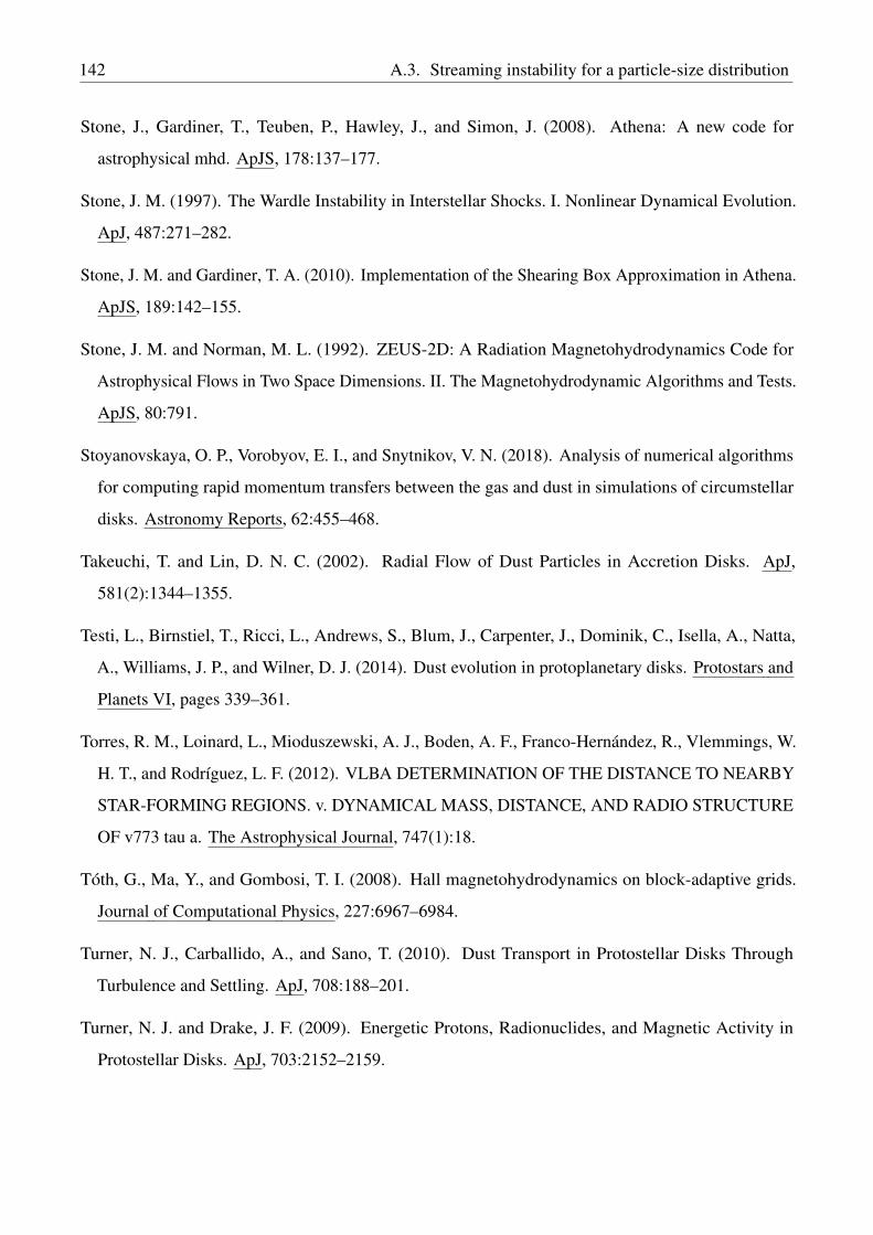
142 A.3. Streaming instability for a particle-size distribution

Stone, J., Gardiner, T., Teuben, P., Hawley, J., and Simon, J. (2008). Athena: A new code for

astrophysical mhd. ApJS, 178:137–177.

Stone, J. M. (1997). The Wardle Instability in Interstellar Shocks. I. Nonlinear Dynamical Evolution.

ApJ, 487:271–282.

Stone, J. M. and Gardiner, T. A. (2010). Implementation of the Shearing Box Approximation in Athena.

ApJS, 189:142–155.

Stone, J. M. and Norman, M. L. (1992). ZEUS-2D: A Radiation Magnetohydrodynamics Code for

Astrophysical Flows in Two Space Dimensions. II. The Magnetohydrodynamic Algorithms and Tests.

ApJS, 80:791.

Stoyanovskaya, O. P., Vorobyov, E. I., and Snytnikov, V. N. (2018). Analysis of numerical algorithms

for computing rapid momentum transfers between the gas and dust in simulations of circumstellar

disks. Astronomy Reports, 62:455–468.

Takeuchi, T. and Lin, D. N. C. (2002). Radial Flow of Dust Particles in Accretion Disks. ApJ,

581(2):1344–1355.

Testi, L., Birnstiel, T., Ricci, L., Andrews, S., Blum, J., Carpenter, J., Dominik, C., Isella, A., Natta,

A., Williams, J. P., and Wilner, D. J. (2014). Dust evolution in protoplanetary disks. Protostars and

Planets VI, pages 339–361.

Torres, R. M., Loinard, L., Mioduszewski, A. J., Boden, A. F., Franco-Hernández, R., Vlemmings, W.

H. T., and Rodríguez, L. F. (2012). VLBA DETERMINATION OF THE DISTANCE TO NEARBY

STAR-FORMING REGIONS. v. DYNAMICAL MASS, DISTANCE, AND RADIO STRUCTURE

OF v773 tau a. The Astrophysical Journal, 747(1):18.

Tóth, G., Ma, Y., and Gombosi, T. I. (2008). Hall magnetohydrodynamics on block-adaptive grids.

Journal of Computational Physics, 227:6967–6984.

Turner, N. J., Carballido, A., and Sano, T. (2010). Dust Transport in Protostellar Disks Through

Turbulence and Settling. ApJ, 708:188–201.

Turner, N. J. and Drake, J. F. (2009). Energetic Protons, Radionuclides, and Magnetic Activity in

Protostellar Disks. ApJ, 703:2152–2159.

A.3. Streaming instability for a particle-size distribution 143

Umebayashi, T. and Nakano, T. (1981). Fluxes of Energetic Particles and the Ionization Rate in Very

Dense Interstellar Clouds. PASJ, 33:617.

van Leer, B. (1977). Towards the Ultimate Conservative Difference Scheme. IV. A New Approach to

Numerical Convection. Journal of Computational Physics, 23:276.

Vorobyov, E. I., Akimkin, V., Stoyanovskaya, O., Pavlyuchenkov, Y., and Liu, H. B. (2018). Early

evolution of viscous and self-gravitating circumstellar disks with a dust component. A&A, 614:A98.

Walt, S. v. d., Colbert, S. C., and Varoquaux, G. (2011). The numpy array: A structure for efficient

numerical computation. Computing in Science and Engg., 13(2):22–30.

Wang, L., Bai, X.-N., and Goodman, J. (2019). Global Simulations of Protoplanetary Disk Outflows

with Coupled Non-ideal Magnetohydrodynamics and Consistent Thermochemistry. ApJ, 874:90.

Wardle, M. (1999). The Balbus-Hawley instability in weakly ionized discs. MNRAS, 307(4):849–856.

Wardle, M. (2007). Magnetic fields in protoplanetary disks. Ap&SS, 311(1-3):35–45.

Wardle, M. and Salmeron, R. (2012). Hall diffusion and the magnetorotational instability in

protoplanetary discs. MNRAS, 422:2737–2755.

Weber, P., Benítez-Llambay, P., Gressel, O., Krapp, L., and Pessah, M. (2018). Characterizing the

variable dust permeability of planet-induced gaps. ApJ, 854:153.

Weidenschilling, S. J. (1977). Aerodynamics of solid bodies in the solar nebula. MNRAS, 180:57–70.

Whipple, F. L. (1972a). On certain aerodynamic processes for asteroids and comets. In Elvius, A.,

editor, From Plasma to Planet, page 211.

Whipple, F. L. (1972b). On certain aerodynamic processes for asteroids and comets. In Elvius, A.,

editor, From Plasma to Planet, page 211.

Williams, J. P. and Cieza, L. A. (2011). Protoplanetary Disks and Their Evolution. ARA&A, 49(1):67–

117.

Windmark, F., Birnstiel, T., Ormel, C. W., and Dullemond, C. P. (2012). Breaking through: The effects

of a velocity distribution on barriers to dust growth. A&A, 544:L16.

Youdin, A. and Johansen, A. (2007). Protoplanetary disk turbulence driven by the streaming instability:

Linear evolution and numerical methods. ApJ, 662:613–626.

144 A.3. Streaming instability for a particle-size distribution

Youdin, A. N. and Goodman, J. (2005). Streaming instabilities in protoplanetary disks. ApJ, 620:459–

469.

Zhu, Z., Nelson, R. P., Dong, R., Espaillat, C., and Hartmann, L. (2012). Dust filtration by planet-

induced gap edges: Implications for transitional disks. ApJ, 755:6.

Ziegler, U. (2004). A central-constrained transport scheme for ideal magnetohydrodynamics. JCoPh,

196:393–416.

Ziegler, U. (2011). A semi-discrete central scheme for magnetohydrodynamics on orthogonal curvilinear

grids. JCoPh, 230:1035–1063.

Ziegler, U. (2016). A chemical reaction network solver for the astrophysics code NIRVANA. A&A,

586:A82.