Widths and Shifts of Isolated Lines of Neutral and Ionized Atoms Perturbed by Collisions With...

Atoms 2014, 2, 225-252; doi:10.3390/atoms2020225OPEN ACCESS

atoms

ISSN 2218-2004www.mdpi.com/journal/atoms

Article

Widths and Shifts of Isolated Lines of Neutral and IonizedAtoms Perturbed by Collisions With Electrons and Ions: AnOutline of the Semiclassical Perturbation (SCP) Method and ofthe Approximations Used for the CalculationsSylvie Sahal-Bréchot 1,*, Milan S. Dimitrijevic 1,2 and Nabil Ben Nessib 3

1 Laboratoire d’Étude du Rayonnement et de la Matière en Astrophysique et Atmosphères (LERMA2),Observatoire de Paris, UMR CNRS 8112, UPMC, 5 Place Jules Janssen, 92195 MeudonCEDEX, France

2 Astronomical Observatory, Volgina 7, 11060 Belgrade, Serbia; E-mail: [email protected] Department of Physics and Astronomy, College of Science, King Saud University. Riyadh 11451,

Saudi Arabia; E-mail: [email protected]

* Author to whom correspondence should be addressed; E-Mail: [email protected];Tel.: +331-450-774-42; Fax: +331-450-771-00.

Received: 24 April 2014; in revised form: 22 May 2014 / Accepted: 26 May 2014 /Published: 10 June 2014

Abstract: “Stark broadening” theory and calculations have been extensively developedfor about 50 years. The theory can now be considered as mature for many applications,especially for accurate spectroscopic diagnostics and modeling, in astrophysics, laboratoryplasma physics and technological plasmas, as well. This requires the knowledge ofnumerous collisional line profiles. In order to meet these needs, the “SCP” (semiclassicalperturbation) method and numerical code were created and developed. The SCPcode is now extensively used for the needs of spectroscopic diagnostics and modeling,and the results of the published calculations are displayed in the STARK-B database.The aim of the present paper is to introduce the main approximations leading to theimpact of semiclassical perturbation method and to give formulae entering the numericalSCP code, in order to understand the validity conditions of the method and of theresults; and also to understand some regularities and systematic trends. This would

Atoms 2014, 2 226

also allow one to compare the method and its results to those of other methodsand codes. 1

Keywords: Stark broadening; impact approximation; isolated lines; semiclassicalperturbation picture

1. Introduction

“Stark broadening” theory and calculations have been extensively developed for about 50 years.Following the pioneering work by [1–4], the theory and calculation of collisional line broadening inthe impact approximation showed a great expansion from the sixties. The theory can now be consideredas mature for many applications, especially for accurate spectroscopic diagnostics and modeling, inastrophysics, laboratory plasma physics and technological plasmas, as well. This requires the knowledgeof numerous collisional line profiles. Hence, calculations based on a simple method that is accurate andfast enough are necessary for obtaining numerous results. In order to meet these needs, the impactsemiclassical perturbation (SCP) method and the associated numerical code were created and developedby Sahal-Bréchot for isolated lines in the sixties and seventies [5–9], then updated [10–12] in the eightiesand nineties and then, again, in the present new century [13]. Since the impact approximation wasassumed, the method was inspired by the developments of the theory of electron-atom and electron-ioncollisions which have been rapidly expanding since the sixties. In particular [14], the semiclassicalperturbation method appeared to be especially suitable, due to the speed of the numerical calculationsand to the sufficient expected accuracy. Nowadays, the SCP code is extensively used for the needs ofspectroscopic diagnostics and modeling, and the results of the published calculations are displayed inthe STARK-B database [15].

The aim of the present paper is to introduce the main approximations leading to the impactsemiclassical perturbation method and to the formulae entering the numerical SCP code. This wouldgive an idea of the validity conditions of the method and of the results, which are discussed in Section 4.This would also allow one to compare the different codes, and this would help to understand someregularities and systematic trends observed in the experiments and in the results of calculations.

In the next section, we will recall the basic key assumptions leading to the theory of collisional linebroadening in impact approximation. We will define the concepts of “complete collision” approximationand of “isolated lines”. Then, we will recall the specific approximations made in the semiclassicalperturbation treatment for isolated lines of neutral and ionized atoms perturbed by electrons and positiveions in the impact approximation. We will give the formulae entering the SCP numerical code. Then,we will discuss the approximations made and the obtained results. This would allow one to compare

1 The content of the present paper was presented and discussed at the first Spectral Line Shapes in Plasmas (SLSP) codecomparison Workshop, which was held in Vienna, Austria, April 2–5, 2012.

Atoms 2014, 2 227

the results obtained by other numerical codes and to understand some regularities and systematic trendsobserved in the experiments and in the results of calculations.

2. Collisional Line Broadening in the Impact Approximation

Following the pioneering work by Baranger [1–4], the theory and calculation of collisional linebroadening widths and shifts in the impact approximation for electrons and ion interactions is verybriefly outlined in the following.

We consider a neutral or ionized atom surrounded by the perturbers, P , moving around it. We beginwith the very general formula [1–4], which gives the intensity, I(!), of a spectral line (i ! f ) at theangular frequency, !:

I(!) =4!4

3c3|hf |d| ii|2 (1)

I(!) =1

2⇡

Z+1

�1exp (i!s) �(s)ds. (2)

Dropping the factor, 4!4/3c3, the autocorrelation function �(s) reads:

�(s) = Tr [dT ⇤(s) dT (s) ⇢]. (3)

Here, ⇢ is the density matrix of the whole system atom (A) surrounded by the bath of particles (B:photons R and perturbers P ), d is the dipole moment, I(!) is the Fourier transform of the autocorrelationfunction, �(s), and T (s) is the evolution operator of the whole system. Tr is the trace over the states ofthe whole system and c is the velocity of the light.

• With the no-back reaction approximation, which is the first key approximation, the bath, B,remains described by its unperturbed density operator (or its distribution function in the classical picture),irrespective of the amount of energy and polarization diffusing into it from A:

⇢(t) = ⇢A(t)⌦ ⇢B(t).

It is also assumed that the bath, B, is in a stationary state, and thus, ⇢B(t) = ⇢B. We also suppose thatthe bath of colliding perturbers P (density matrix ⇢P ) is decoupled from the bath of photons R (densitymatrix ⇢R). Thus:

⇢B = ⇢P ⌦ ⇢R,

and we will only consider in the following the interaction with the bath of colliding particles. Hence, wecan write:

�(s) = TrA [⇢A TrP [dT ⇤(s)dT (s) ⇢P ]] (4)

where TrA is the trace over the atomic states and TrP is a trace over all the perturbers. When theperturbers can be treated classically, the trace over the perturbers is replaced by a statistical average[...]AV over all modes of motion of the perturbers, which move on a classical path [4]:

�(s) = TrA [⇢A dT ⇤(s)d T (s)]AV . (5)

Atoms 2014, 2 228

• The second key approximation is the impact approximation: the interactions are separated in time.In other words, the atom interacts with one perturber only at a given time: the mean duration, ⌧ , ofan interaction must be much smaller than the mean interval between two collisions, �T . This can beexpressed as:

⌧ ⌧ �T,

where ⌧ ⇡ ⇢typvtyp

, ⇢typ is a mean typical impact parameter and vtyp a mean typical relative velocity.�T is of the order of the inverse of the collisional line width, which can be very roughly written as

equal to NP vtyp⇢2

typ, where NP is the density of the perturbers.Thus, the validity condition of the impact approximation can be written as:

⇢typ << N�1/3P . (6)

The “collision volume”, of the order of ⇢3typ, must be smaller than N�1

P , the volume perperturber [1]. In other words, the perturbers are independent and their effects are additive.

• Then, we will make the complete collision approximation: within this approximation,atom–radiation and atom–perturber interactions are decoupled. This implies that the collision mustbe considered as instantaneous in comparison with the time, ��1, characteristic of the evolution of theexcited state under the effect of the interaction with the radiation. In other words, the interaction processhas time to be completed before the emission of a photon.

The complete collision approximation can become invalid in line wings, even if it remains valid inthe line center. Its condition of validity is:

⌧ << 1/�!,

where �! is the detuning.Then, using Equation (4) in the quantum picture or Equation (5) in the semiclassical picture, the

calculation of the line profile becomes an application of the theory of atomic collisions. This impliesthat we have to express and calculate the scattering S-matrix.

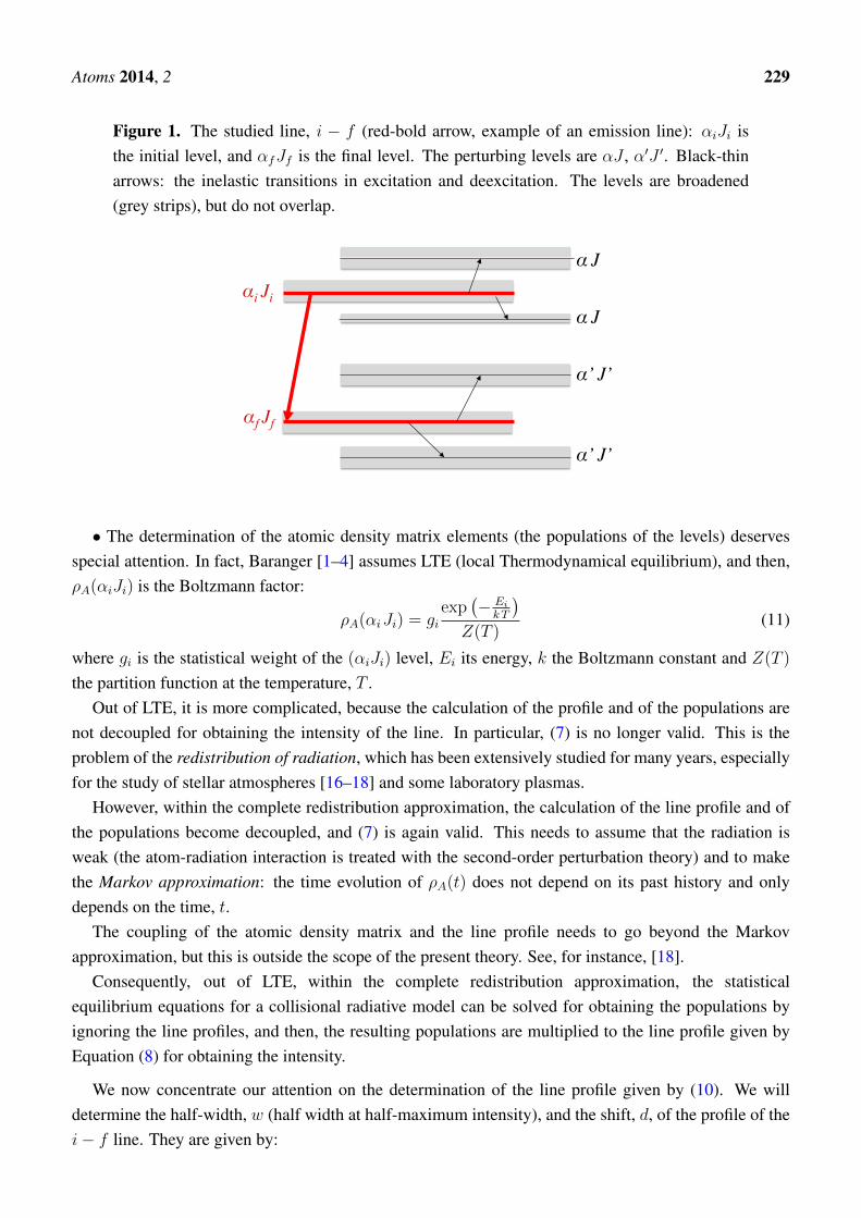
• In addition, in the case of isolated lines (cf. Figure 1), which implies that neighboring levels do notoverlap [3], the line profile, F (!), between the levels, i, (↵iJi) and f (↵fJf ), is Lorentzian:

I(!) = ⇢A (↵iJi)4!4

3c3F (!) (7)

F (!) =1

⇡

Z 1

0

ei(!�!if)s � (s) ds (8)

� (s) = exp (� (w + id) s) (9)

andF (!) =

w

⇡⇥(! � !if � d)2 + w2

⇤ (10)

⇢A is the reduced atomic density matrix at the stationary state.

Atoms 2014, 2 229

Figure 1. The studied line, i � f (red-bold arrow, example of an emission line): ↵iJi isthe initial level, and ↵fJf is the final level. The perturbing levels are ↵J , ↵0J 0. Black-thinarrows: the inelastic transitions in excitation and deexcitation. The levels are broadened(grey strips), but do not overlap.

!"#$%&'()*%+,"-(

!i Ji

!f Jf

! J

! J

!’ J’

!’ J’

• The determination of the atomic density matrix elements (the populations of the levels) deservesspecial attention. In fact, Baranger [1–4] assumes LTE (local Thermodynamical equilibrium), and then,⇢A(↵iJi) is the Boltzmann factor:

⇢A(↵iJi) = giexp

�� Ei

kT

�

Z(T )(11)

where gi is the statistical weight of the (↵iJi) level, Ei its energy, k the Boltzmann constant and Z(T )

the partition function at the temperature, T .Out of LTE, it is more complicated, because the calculation of the profile and of the populations are

not decoupled for obtaining the intensity of the line. In particular, (7) is no longer valid. This is theproblem of the redistribution of radiation, which has been extensively studied for many years, especiallyfor the study of stellar atmospheres [16–18] and some laboratory plasmas.

However, within the complete redistribution approximation, the calculation of the line profile and ofthe populations become decoupled, and (7) is again valid. This needs to assume that the radiation isweak (the atom-radiation interaction is treated with the second-order perturbation theory) and to makethe Markov approximation: the time evolution of ⇢A(t) does not depend on its past history and onlydepends on the time, t.

The coupling of the atomic density matrix and the line profile needs to go beyond the Markovapproximation, but this is outside the scope of the present theory. See, for instance, [18].

Consequently, out of LTE, within the complete redistribution approximation, the statisticalequilibrium equations for a collisional radiative model can be solved for obtaining the populations byignoring the line profiles, and then, the resulting populations are multiplied to the line profile given byEquation (8) for obtaining the intensity.

We now concentrate our attention on the determination of the line profile given by (10). We willdetermine the half-width, w (half width at half-maximum intensity), and the shift, d, of the profile of thei� f line. They are given by:

Atoms 2014, 2 230

w + id = TrP�1� Sii S

⇤ff

�(12)

where the trace over the perturbers, TrP , is given by:

TrP = NP

Z 1

0

vf(v)dv

Z 1

0

2⇡ ⇢ d⇢

Id⌦

4⇡. (13)

Equation (13) is written in the semiclassical picture, where the colliding perturbers move along aclassical path of impact parameter ⇢, but this is not essential. Here, v is the relative velocity of theperturber, f(v) the distribution of velocities (Maxwell distribution) and NP the density of the perturbers.

Id⌦

4⇡

is the angular average over all directions of the colliding perturbers. Hence:

w + id = NP

R10

vf(v)dvR10

2⇡⇢ d⇢⌦1� Sii S

⇤ff

↵angular average

(14)

This angular average is a linear combination of products of “3-j” coefficients and of initial and finalZeeman states of the S-matrix elements [3]. Thus, Equation (14) reads:

w + id = NP

R10

vf(v)dvR10

2⇡⇢ d⇢

⇥ [1 �P

Mi M0i

Mf M 0f

µ

(�1)2Jf+Mf+M 0f

Ji 1 Jf

�Mi µ Mf

! Ji 1 Jf

�M 0i µ M 0

f

!

⇥⌦↵fJfMf |S⇤ |↵fJfM

0f

↵h↵iJiMi |S |↵iJiM

0ii⇤

(15)

This is the basic “Baranger’s formula” which gives the half-width and the shift of an isolated lineperturbed by collisions (i.e., impact and complete collision approximation). We notice that the S-matrixis symmetric, unitary and can be calculated in any reference frame. Its matrix elements have to becalculated for a given relative velocity, v, and an impact parameter, ⇢, in the semiclassical description.This will appear in the following equations.

In fact, the T -matrix, where T = 1�S (and, thus, T ⇤T = 2Re(T )), is used in the SCP method. Thus,we will use it in the following.

After elementary calculations using the properties of the “3-j” coefficients, Equation (15) reads:

w + id = NP

R10

vf(v)dvR10

2⇡⇢ d⇢

⇥"PMi

1

2Ji+1

h↵iJiMi|T (⇢, v) |↵iJiMii +PMf

1

2Jf+1

h↵f Jf Mf |T ⇤(⇢, v) |↵f Jf Mf i

�P

MiM0i

Mf M 0f

µ

(�1)2Jf+Mf+M 0f

Ji 1 Jf

�Mi µ Mf

! Ji 1 Jf

�M 0i µ M 0

f

!

⇥ h↵iJiMi|T (⇢, v) |↵iJiM 0ii h↵f Jf Mf |T ⇤(⇢, v) |↵f Jf M 0

f i]

(16)

Atoms 2014, 2 231

Then, the half-width at half-maximum intensity w, and the full width at half-maximum intensityW = 2w become:

W = 2w = NP

Rvf(v)dv

⇥✓P

↵J

� (↵iJi ! ↵J, v) +P↵0J 0

� (↵fJf ! ↵0J 0, v)

◆

� 2ReR10

2⇡⇢ d⇢ [P

Mi M0i

Mf M 0f

µ

(�1)2Jf+Mf+M 0f

⇥

Ji 1 Jf

�Mi µ Mf

! Ji 1 Jf

�M 0i µ M 0

f

!

⇥⌦↵fJfMf |T ⇤(⇢, v) |↵fJfM

0f

↵h↵iJiMi |T (⇢, v) |↵iJiM

0ii⇤

(17)

In Equation (17):

X

↵J

� (↵iJi ! ↵J, v)

is a sum of all the inelastic cross-sections originating from the initial level towards all perturbing levels,↵J , in excitation and deexcitation (cf. Figure 1), with ↵iJi 6= ↵J , and of the elastic cross-section�(↵iJi ! ↵iJi, v).

In fact:� (↵iJi ! ↵J, v) =

Z 1

0

2⇡⇢ d⇢ P (↵iJi ! ↵J, ⇢, v) (18)

where P (↵iJi ! ↵J, ⇢, v) is the transition probability between the levels, (↵iJi) and (↵J), for theimpact parameter, ⇢, and the relative velocity, v.

We have similar expressions for the inelastic cross-sections originating from the final level ↵fJf .Then the perturbing levels are ↵0J 0 and the elastic cross-section is �(↵fJf ! ↵fJf , v).

We notice that the transition probability:

P (↵iJi ! ↵J, ⇢, v) =1

2Ji + 1

X

MiM

|h↵iJiMi |T (⇢, v) |↵JMi|2 (19)

is a sum over the final M substates and an average over the initial Mi substates of the T -matrix elements.The third term of Equations (16) and (17) is the so-called “interference term", which is a linear

combination of off-diagonal elastic elements of the initial and final elastic elements of the T -matrix. Forcollisions with electrons, it is often small (10% of the total width or thereabout), but not always.

Equations (16) and (17) will be used in the SCP method and numerical code.Finally, we notice that the fine structure (and, a fortiori, hyperfine structure) can generally be ignored,

and consequently, the fine structure components (or hyperfine components) have the same width and thesame shift, which are equal to those of the multiplet. This is due to the fact that the electronic spin, S (ornuclear spin I), has no time to rotate during the collision time (of the order of ⇢/v, the mean duration ofthe collision). This is only true in LS coupling.

Atoms 2014, 2 232

3. The Semiclassical Perturbation Approximation (SCP) for Stark-Broadening Studies

We study the case of isolated lines in the impact and complete collision approximations recalled inthe preceding section.

Within the semiclassical approximation, the perturbers (electrons or positive ions) are assumed to beclassical particles, and they move along a classical path unperturbed by the interactions with the radiatingatom. The atom is described by its quantum wave-functions and energy levels. With the perturbationapproximation, the atom–perturber interaction is treated by the time-dependent perturbation theory. Thelong-range approximation will be made.

3.1. The Semiclassical Approximation and the Parametric Representation of the Orbits

For neutral radiating atoms, the trajectory is rectilinear, and for radiating ions, it is a hyperbola. Theparametric representation of the trajectory can be found in [19] for the repulsive case and also in [6]for the attractive case and the straight path case. The radiating atom is at the origin, O, of the axes.The quantization axis, Oz, is perpendicular to the collision plane, xOy, and the velocity vector of theperturber is parallel to Ox at time t = �1. ZA is the charge of the radiating atom (ZA = 0 for aneutral), ZP the charge of the perturber (ZP = 1 for an electron), µ the reduced mass of the systematom–perturber, v the relative velocity and ⇢ the impact parameter.

The coordinates are given in Table 1.

Table 1. Parametric representation of the orbits (trajectories).

Attractive Hyperbola Repulsive Hyperbola Straight Path

x a ("� cosh u) a ("+ coshu) ⇢

y ap"2 � 1 sinh u a

p"2 � 1 sinh u ⇢ sinh u

t av(" sinh u� u) a

v(" sinh u+ u) ⇢

vsinh u

distance of closest approach a("� 1) a("+ 1) ⇢

For radiating ions, a = e2ZAZP

µ v2is the semi-major axis of the hyperbola, e is the electron charge and

" =⇣1 + ⇢2

a2

⌘ 12 is the eccentricity.

3.2. The Time-Dependent Perturbation Approximation for the Calculation of the S (or T ) Matrix

We use the following expression for the S-matrix:

S = T✓exp

✓1

ih

Z+1

�1V (t) dt

◆◆(20)

where T is the chronological operator and V (t) is the atom–perturber interaction potential in interactionrepresentation. Now, we make the second order perturbation theory: we expand the S�matrix given

Atoms 2014, 2 233

by Equation (20) in multipoles (the so-called Dyson series), and we retain the two first terms of theexpansion:

S = 1 +1

ih

Z+1

�1V (t)dt+

1

i2h2

Z+1

�1V (t)dt

Z t

�1V (t0)dt0 (21)

and T follows:

T = +i

h

Z+1

�1V (t)dt+

1

h2

Z+1

�1V (t)dt

Z t

�1V (t0)dt0. (22)

3.3. The Atom-Perturber Interaction Potential

We will only study the case of an ideal plasma, which is valid if the Debye length is much largerthan the mean distance between perturbers. Hence the atom–perturber interaction V is the electrostaticpotential between the N atomic electrons, the nucleus of charge (ZA + N ) and the perturber of charge,ZP (with ZP = �1 for an electron):

V =(ZA +N)ZP e2

rP� ZP e2

NX

i=1

1

riP(23)

where rP is the distance between the nucleus and the perturber and riP the distance between the ith

atomic electron and the perturber. ZA = 0 for a neutral atom.Then, 1/riP is expanded into multipolar components. We will only retain the long range part, since

we will make the long-range perturbation theory. Penetrating orbits are outside the scope of SCP methodand code. The Y�µ denote the spherical harmonics.

V =ZA ZP e2

rP�

1X

�=1

4⇡ZP e2

2�+ 1

1

r�+1

P

+�X

µ=��

NX

i=1

r�i Y�µ(rP )Y⇤�µ(ri). (24)

The first term of this expansion is the Coulomb term, which does not play any role in the calculationof the S-matrix, due to its spherical symmetry. The following ones have to be retained: the dipole term(� = 1) and the quadrupole term (� = 2).

3.4. Determination of the T -Matrix Elements Using Equations (22) and (24) and the Coordinates ofthe Perturber

Thanks to the preceding subsections, we are now able to obtain the semiclassical perturbationexpressions of Equations (16) and (17). The T�matrix elements, which enter Formula (16), read:

h↵iJiMi|T (⇢, v) |↵iJiM0ii = i

h

R+1�1 h↵iJiMi|V (⇢, v, t) |↵iJiM

0ii dt

+ 1

h2

P↵JM

R+1�1 h↵iJiMi|V (⇢, v, t) |↵JMi ei!ijtdt

R t

�1 h↵JM |V (⇢, v, t0) |↵iJiM0ii e�i!ijt

0dt0

,

(25)where !ij is the angular frequency difference between the initial i (↵iJi) level and the perturbing j (↵J)level. We have an analogous expression for the final f (↵fJf ) level.

Atoms 2014, 2 234

The first term of Equation (16) is the first direct term, originating from the initial level. It reads:PMi

h↵iJiMi|T (⇢, v) |↵iJi Mii = i

h

PMi

R+1�1 h↵iJiMi|V (⇢, v, t) |↵iJiMii dt

+ 1

h2

P↵JMMi

R+1�1 h↵iJiMi|V (⇢, v, t) |↵JMi ei!ijtdt

R t

�1 h↵JM |V (⇢, v, t0) |↵iJiMii e�i!ijt0dt0

(26)The second term of Equation (16) is the second direct term, originating from the final level, ↵Jf , and

has an analogous expression.The third term of Equation (16) is the interference term.Then, we use the second order long-range expansion of the interaction potential (Equation (24)). We

do not enter the details of the calculations, which can be found in Sahal-Bréchot [6].We summarize the different steps and only give the resulting formulae in the following:

• The quadrupolar potential is taken into account only for elastic collisions and for inelastic collisionsbetween the fine structure levels of the initial and final levels.

• The fist term of Equation (26) is taken as equal to zero:�It is exactly equal to zero for the (� = 1)-dipolar potential contribution, due to selection rules on

the “3j” coefficients.�It is only different from zero for the (� = 2)-quadrupolar potential contribution in the case of

Ji � 1 integer numbers, but is neglected.

• The second term of Equation (26) contains quadrupolar and dipolar elements.

• There is no interference terms between dipolar and quadrupolar contributions, which addindependently.

• The Debye screening is taken into account by introducing an upper cutoff at the Debye length. Thecalculations are detailed in [6] for obtaining the T�matrix elements and in [7] for the integration overthe impact parameters and the choice of the cutoffs.

The full width at half-maximum intensity, W , and the shift, d, of the i � f line can be put underthe form [7]:

W = NP

Zvf(v)dv

X

i0 6=i

�ii0(v) +X

f 0 6=f

�ff 0(v) + �el

!(27)

Here, the perturbing levels are denoted as i0 and f 0 for simplicity in the writing.• The inelastic contribution of the upper level, i, is calculated as follows [7]. The dipolar interaction

potential is taken into account:

X

i0 6=i

�ii0(v) =1

2⇡R2

1

+

Z RD

R1

2⇡⇢d⇢X

i0 6=i

Pii0(⇢, v) (28)

Pii0(⇢, v) =1

h2

��Z

+1

�1Vii0 exp

✓� i

h�Eii0 t

◆��2

(29)

Atoms 2014, 2 235

with �Eii0 = h!ii0 .The upper cutoff, RD, is the Debye radius. The lower cutoff, R

1

, is chosen as in [7,14]:X

i0 6=i

Pii0(⇢, v) =1

2

or, in the case of electron collisions:X

i0 6=i

�ii0(v) =

Z RD

min(hrii,hri0i)2⇡⇢d⇢

X

i0 6=i

Pii0(⇢, v) (30)

where hrii is the mean radius of the i level and hri0i is the mean radius of the i0 level. An hydrogenicapproximation is sufficient for calculating these mean radii, and we retain as in [14] the smallest resultbetween the one of Equation (29) and the one of Equation (30). This minimizes [14] the role of closecollisions, which are considered as overestimated by the perturbation theory.

In the case of collisions with positive ions (cf. [20]), we retain the smallest between the result ofEquation (28) and of the following one:

X

i0 6=i

�ii0(v) = ⇡hrii2Pii0 (hrii , v) +Z RD

hrii2⇡⇢d⇢

X

i0 6=i

Pii0(⇢, v) (31)

The inelastic contribution from the lower level, f , is calculated in the same way.

• The contribution of elastic collisions, �el, is calculated as follows:

�el = 2⇡R2

2

+

Z RD

R2

2⇡⇢d⇢ sin2 '+ �r (32)

with:' = ('2

p + '2

q)12 (33)

and:'p =

X

i0 6=i

'ii0 �X

f 0 6=f

'ff 0 (34)

The phase shifts, 'p and 'q, are due, respectively, to the dipolar potential (the polarization potential inthe adiabatic approximation) and to the quadrupolar potential. The contribution of the dipolar interactionto the width is often denoted as the quadratic contribution. Their expressions will be detailed hereafter.The lower cutoff, R

2

, is chosen as '(R2

, v) = 1 [7]. The interference term is taken into account in 'p

and 'q.Here, �r is the contribution of the Feshbach resonances [9], which concerns only ionized radiating

atoms colliding with electrons. It is an extrapolation of the excitation collision strengths (and not thecross-sections) under the threshold by means of the semiclassical limit of the Gailitis approximation(see [9] for details of the calculations).

• The shift, d, is given by (the dipolar interaction potential is the only one to be taken into account):

d = NP

Zvf(v)dv

Z RD

R3

2⇡⇢d⇢ sin(2'p) (35)

The cutoff, R3

[7], is chosen as 2'p(⇢, v) = 1. There is no strong collision term for the shift.

Atoms 2014, 2 236

3.5. Expressions of Pii0(⇢, v), Pff 0(⇢, v),'p(⇢, v),'q(⇢, v), Symmetrization and Some Asymptotic Limits

We use CGS units, but we will often use atomic units (h = 1, e = 1, me = 1, and thus, a0

= 1,IH = 1/2):a0

= h2

me e2is the first Bohr orbit radius, me is the electron mass and e the electron charge. IH = me e4

2 h2 isthe ionization energy of hydrogen (1 Rydberg).

3.5.1. Case of Neutral Atoms (Straight Path)

Contribution of the dipolar interaction: expressions of the transition probabilities, of the inelasticcross-sections and of 'p

1

2Pii0(⇢, v) + 2 i'ii0 (⇢, v) =

a20

⇢22 I2H

E�Eii0fii0

µ

me

Z2

P (A(z) + iB(z)) (36)

z =⇢�Eii0

h v, fii0 is the oscillator strength of the (ii0) transition, and E = 1

2

µ v2 is the incident kineticenergy of the perturber.

A(z) + iB(z) =1

2

Z+1

�1du

Z u

�1du0✓1 + sinh u sinh u0

cosh2u cosh2u0 exp (iz (sinh u� sinh u0))

◆(37)

A(z) and B(z) are connected together by the Hilbert transform:

B(z) = 1

⇡pvR

+1�1 dz0A(z0)

z�z0

A(z) = 1

⇡pvR

+1�1 dz0B(z0)

z�z0

where pv denotes the Cauchy principal value.A(z) can be expressed by means of the modified Bessel functions, K

0

and K1

[14]:

A(z) = z2�|K

0

(z)|2 + |K1

(z)|2�

(38)

and the expression of B(z) was obtained by [21]:

B(z) = ⇡ z2 (|K0

(z)| |I0

(z)|� |K1

(z)| |I1

(z)|) . (39)

Then, we integrate over the impact parameter for obtaining the inelastic, ii0, contribution:

Z RD

R1

2⇡⇢ d⇢ Pii0(⇢, v) = ⇡a20

8 I2HE�Eii0

fii0µ

me

Z2

P (a(zD)� a(z1

)) (40)

with [14]:a(z) = z |K

1

(z)|K0

(z).

Symmetrization

We now introduce the symmetrization of the transition probabilities and cross-sections, in order tosatisfy the reciprocity relations [14]. We replace E by Esym and z by zsym:

Esym =1

2(2E ��Eii0) (41)

Atoms 2014, 2 237

zsym =⇢

a0

rµ

me

rE

IH

�Eii0

2E ��Eii0. (42)

Remark concerning the shift

Note that in the SCP method and computer code, we calculate the shift with Equation (35). Thus, theintegration over the impact parameter is not analytical. However, we have also calculated the shift withthe more usual formula, where the b(z) function [21] appears:

Z RD

R4

2⇡⇢ d⇢ 2'ii0(⇢, v) = ⇡a20

4 I2HE�Eii0

fii0µ

me

Z2

P (b(zD)� b(z4

)) (43)

b(z) =⇡

2� ⇡zK

0

(z)I1

(z) (44)

In that case, we have chosen the lower cutoff, R4

, as equal to 1

2

(hrii+ hrfi) where hrii is the meanradius of the i level and hrfi the mean radius of the f level. In fact, the obtained results are quite sensitiveto the cutoff, and we have preferred our method of calculation given by Equation (35). Therefore, ourshift results with the b(z) function appear neither in our publications nor in the STARK-B database.

Asymptotic limits and series expansions of A(z), a(z), B(z)

The asymptotic limits of A(z), B(z) and a(z) are recalled hereafter, because they are useful forunderstanding some systematic trends: At high energies (or very small �E):

A(z) ! 1, @A@z

! zero,a(z) ! ln

⇣2

�z

⌘and

B(z) ! 0 and @B@z

! zero.� = expC and C = 0.5772156649 is the Euler constant.At low energies (or high �E): A(z) ! ⇡z exp(�2z), B(z) ! ⇡/4z + 9⇡/32z2 + ... and a(z) !

⇡2

exp(�2z).In fact, at low energies, the Lindholm limit due to a polarization potential of the phase shift, 'p, is

obtained (cf. [22]). The limit (� ! 0) is 'p = 'i � 'f , with:

'i =X

i0 6=i

⇡

2Z2

P

✓a0

⇢

◆3

rIHE

rµ

me

fii0

✓IH

�Eii0

◆

with an analogous expression for 'f . Contribution of the quadrupolar interaction: expression of 'q

This only concerns the elastic term of the width (cf. above). The contribution of the inelastictransitions between fine structure levels of the initial and final level (if any) are included in the elasticterm. The details of the calculations are given in [6], in [8] for the Bi, Bf , Bif angular coefficients ofcomplex atoms and in [13] for still more complex atoms. We have [6]:

'2

q =h�Bi

⌦r2i↵�

2

+�Bf

⌦r2f↵�

2 � Bif

⌦r2i↵ ⌦

r2f↵i

Z2

P

µ

me

a40

⇢4IHE

(45)

In the SCP computer code, the calculations of the Bessel functions use the Fortran library of [23].The integration over the impact parameter of the elastic part of the width and of the shift use Gauss

Atoms 2014, 2 238

integration techniques and Gauss–Laguerre integration techniques for the integration over the Maxwelldistribution of velocities. The Gauss–Laguerre technique is not suitable for the inelastic part, because athigh energies, the inelastic dipolar cross-sections decrease as (lnE)/E. A trapezoidal method with anincreasing exponential step is used; it is suitable and accurate.

3.5.2. Case of Ionized Atoms (Hyperbolic Path)

Contribution of the dipolar interaction: expressions of the transition probabilities, of the inelasticcross-sections and of 'p

We define:

⇠ =a�Eii0

hv=

1

2ZA ZP

rµ

me

�Eii0

IH

✓IHE

◆ 32

and we obtain:

1

2Pii0(", v) + 2 i'ii0(", v) =

a20

(a")22 I2H

E�Eii0fii0

µ

me

Z2

P (A(⇠, ") + iB(⇠, ")) (46)

A(⇠, ") = (⇠")2 exp(±⇡⇠)

✓|K

i⇠(⇠")|2 +"2 � 1

"2��K 0

i⇠(⇠")��2◆

(47)

where ± means + for the attractive case and � for the repulsive case.We recognize the Bessel functions of imaginary order i⇠ and real argument ⇠":

Ki⇠(⇠") =

R10

e�⇠ " coshu cos⇠u du

K 0i⇠(⇠") =

R10

e�⇠ " coshu cos⇠u cosh u du(48)

As for the straight path case, A(⇠, ") and B(⇠, ") are connected together by the Hilbert transform, butnow, the variable is ⇠:

B(⇠, ") =1

⇡pv

Z+1

�1d⇠0

A(⇠0, ")

⇠ � ⇠0(49)

Contrary to the straight path case, we do not know any other analytical formula for B(⇠, ").Therefore, it will be calculated numerically by using asymptotic formulae, which will begiven hereafter.

For the attractive case, B(⇠, ") has also been calculated by use of the Hilbert transform whenasymptotic formulae are not adequate. However, Equation (49) is not suitable for numerical calculations.In the SCP computer code, the dispersion relation has been used:

B(⇠, ") =1

⇡

Z+1

0+

d⇠0A(⇠ � ⇠0, ")� A(⇠ + ⇠0, ")

⇠0(50)

and also the second imaginary term of the Dyson series:

B(⇠, ") = 1

2

R+1�1 du

R u

�1 du0 [sin [⇠ ("(sinh u� sinh u0)� (u� u0)]

⇥ "2+("2�1) sinhu sinhu0+coshu coshu0�"(coshu+coshu0

)

(" coshu�1)

2(" coshu0�1)

2

i (51)

Atoms 2014, 2 239

The integration over the impact parameter of the transition probability, Pii0(⇠, "), has ananalytic solution:

Z RD

R1

2⇡⇢ d⇢X

i0 6=i

Pii0(⇢, v) = 8⇡a20

2 I2HE�Eii0

fii0µ

me

Z2

P (a(⇠, "D)� a(⇠, "1

))

with:a(⇠, ") = exp(±⇡⇠) ⇠"K

i⇠(⇠")K0i⇠(⇠") (52)

where ± means + for the attractive case and � for the repulsive case.Sample graphs of the A(⇠, "), a(⇠, ") and B(⇠, ") functions are displayed in [5,24,25].

Symmetrization of the transition probabilities and cross-sections

As for the straight path case, the transition probabilities and cross-sections are also symmetrized[7,19,24].

a and ⇠ become asym and ⇠sym, with Ei = E, E 0i = Ei +�Eii0 :

asym = a0

IHZA ZPpEiEi0

and

⇠sym = ZAZP

qµme

⇣qIHEi

�q

IHEi0

⌘.

Asymptotic and series expansions for A, a and B, used in the computer code

(1) First, we recall that:A (0, ") = 1@A@⇠

(0+, ") = ±⇡

with ±: + for the attractive case and � for the repulsive case.

B (0, ") = 1@B@⇠

(0+, ") = ⌥1

with ⌥: � for the attractive case and + for the repulsive case.

(2) At high energies, E, or small �Eii0 , ⇠ ! zero, one obtains:

a(⇠, �) = (1± ⇡⇠) ln

✓2

� + �

◆(53)

with � = ⇠(" � 1) and with � = eC . C is the Euler constant. We haveused this asymptotic expression for calculating A(⇠, �) and a(⇠, �) for ⇠ < 0.1 and for� < 0.025.

At very high energies, the Coulomb attraction (or repulsion) becomes weak; the contribution ofhigh impact parameters predominates, ⇠" ! ⇢, and the straight path case is recovered.

Atoms 2014, 2 240

(3) For high ⇠ and high ⇠", the following asymptotic expansion—valid for order and argument bothhigh and nearly equal ([26] p. 245 and [27] p. 88, [28], such as � = ⇠"� ⇠ = o(⇠")1/3)—has beenused:

Ki⇠ (⇠") =

1

3

e�⇡⇠2

1Pm=0

sin⇣

(m+1)⇡3

⌘��m+1

3

� �⇠"6

��m+13 Am

K 0i⇠ (⇠") =

1

6

e�⇡⇠2

1Pm=0

sin⇣

(m+1)⇡3

⌘��m+1

3

� �⇠"6

��m+13 A0

m

+1

3

e�⇡⇠2

1Pm=0

sin⇣

(m+1)⇡3

⌘��m+1

3

� �⇠"6

��m+43��m+1

18

�Am

(54)

We have expanded the series up to m = 4 [28] in the SCP code. The Am and A0m coefficients are

given in Table 2.

Table 2. Values of the coefficients Am and A0m in Equation (54) [28].

m Am A0m

0 1 0

1 �� 2

2 �2/2 + 1/20 2�

3 ��3/6� �/15 ��2 � 2/15

4 �4/24 + �2/24 + 1/280 �3/3 + �/6

Note that there is a typo in [28]. Therefore, the correct formulae are:

Ki⇠ (⇠") =

p3

6

e�⇡⇠2

⇥��1

3

� ⇣6

⇠"

⌘ 13 � �

�2

3

� ⇣6

⇠"

⌘ 23� + �

�4

3

� ⇣6

⇠"

⌘ 43 �3

(0.5�2 + 0.2)

� ��5

3

� ⇣6

⇠"

⌘ 53⇣

�4+�2

3

+ 1

35

⌘�

K 0i⇠ (⇠") =

p3

12

e�⇡⇠2

⇣6

⇠"

⌘ 23

2��2

3

�+⇣

6

⇠"

⌘ 23 ��

�4

3

� ��2 + 2

15

��

+ 1

9

��1

3

�+⇣

6

⇠"

⌘ ��5

3

��6

(1 + �2)� 2

9

��2

3

��i

(55)

(4) When " ! 1 (or � ! 1), we have used the expansion ([26] p. 202):

Ki⇠ (⇠") =

⇣⇡

2⇠ "

⌘ 12e�⇠"

1Pk=0

(�4⇠2�1)(�4⇠2�9)...(�4⇠2�(2k�1)

2)k! (8⇠ ")k

�

K 0i⇠ (⇠") = �

⇣⇡

2⇠ "

⌘ 12e�⇠"

1Pk=0

(�4⇠2+16k2�1)...(�4⇠2�(2 (2k�1)�1)

2)(2k)! (8⇠ ")k

+1Pk=0

(�4⇠2+4(2k+1)

2�1)...(�4⇠2�(4k�1))

2)(2k+1)! (8⇠ ")2k+1

�

(56)

We have used this expansion for calculating A(⇠, �) and a(⇠, �) for ⇠ < 10 and � > 90.

(5) Beyond the validity of these above expansions, the Ki⇠(⇠, �) and K 0

i⇠(⇠, �) functions havebeen calculated with an unpublished Fortran subroutine developed in [24]. The A(⇠, �) anda(⇠, �) follow.

Atoms 2014, 2 241

(6) Asymptotic expansions for B(⇠, ") for the attractive case (collisions with electrons).

We have used two expansions. The first one is valid for high values of ⇠, and the first two termswere calculated by [6]. We have added the third term of the expansion in the numerical SCP code.It reads:

B(⇠, ") = "2

2⇠("2�1)

2

3 + (2 + "2)

⇡�arccos( 1")p

"2�1

�

+ "2

16⇠3("2�1)

5

124+592 "2+229"4

3

+ (16 + 152"2 + 138"4 + 9"6)⇡�arccos( 1

")p"2�1

�

+ "2

256⇠5("2�1)

8

h4576+144160 "2+539524"4+392088"6+45777"8

5

+ (256 + 13952"2 + 82752"4 + 101600"6 + 25990"8 + 675"10)⇡�arccos( 1

")p"2�1

�

(57)

For " < 1.01, we have used the expansion derived by [29], and we have limited it to the first twoterms in the SCP code. It reads:

B (⇠, ") =p3⇡ "

32 ⇠

23

⇣� 0.940 + 2.228 ("� 1) ⇠

23

⌘. (58)

For high values of ⇠ and high values of ", we have used the asymptotic form:

B (⇠, ") =3⇡"2

2⇠("2 � 1)52

=2⇡a5

3 ⇠⇢5. (59)

(7) Beyond the validity of these expansions, B(⇠, ") has been calculated by means of a numericalintegration of the Hilbert transform (Equation (50)) or by a numerical integration of the secondimaginary term of the Dyson series (Equation (52)).

(8) Asymptotic expansions for B(⇠, ") for the repulsive case (collisions with positive ions).

Due to the mass effect, ⇠ is always high in typical conditions for Stark broadening studies.Therefore, an expansion valid for high values of ⇠ is sufficient and has been introduced in theSCP computer code. It reads [6]:

B (⇠, ") ="2

2⇠ ("2 � 1)

✓2 + "2p"2 � 1

arccos

✓1

"

◆� 3

◆+ (...) . (60)

If in addition, " ! 1:

B (⇠, ") ="2

2⇠

✓2

15� 4

35

�"2 � 1

�+

2

21

�"2 � 1

�2 � 8

99

�"2 � 1

�3

+ ...

◆. (61)

Contribution of the quadrupolar interaction: expression of 'q for radiating ions

After an elementary calculation, one obtains [6]:

'2

q =h(Bi hr2i i)

2

+�Bf

⌦r2f↵�

2 � Bif hr2i i⌦r2f↵i

µme

Z2P

(a2"2)2IHE

⇥1

4

+ 3 "4

4("2�1)

2

✓1 +

⌥⇡+2arcsin( 1")

2

p"2�1

◆� (62)

Atoms 2014, 2 242

where ⌥ means + for the attractive case and � for the repulsive case.At high eccentricities or high energies (as expected), we recover the straight path limit.

At low energies and small eccentricities, by using the series expansion of arcsin 1/", weobtain [6] the asymptotic phase shift found in [22] for electron collisions.

4. Results and Discussion

4.1. Validity of the Impact Approximation

The impact approximation is at the basis of the SCP method. Its validity is checked in all of thecalculations for every line, every temperature and every density by using Equation (6).

The collision volume is calculated by writing W = NPvtyp⇢2

typ, where W is the calculated width, NP

the density of the perturbers and vtyp is the mean relative velocity. Thus, ⇢typ can be derived. One of theoutputs of the code is NPV , where V = ⇢3typ is the collision volume.

We give, in the following (Tables 3–6), two examples. Table 3 (electron collisions) and Table 4(proton collisions) concern the case of Ne VIII 3s� 3p at 1019 cm�3. The data are taken from the casesstudied at the Spectral Line Shapes in Plasmas workshop (April, 2012). Table 5 (electron collisions) andTable 6 (proton collisions) concern the case of Li I 2s� 2p at 1016 cm�3.

The results for NPV show that the impact approximation is valid both for electron and proton collidersin these two cases.

In the STARK-B database, the values of the widths and shifts are provided in the tables, except whenNPV > 0.5, where the cells are empty and marked with an asterisk preceding the cell. Widths and shiftsvalues for 0.1 < NPV < 0.5 are given and marked by an asterisk in the cell preceding the value.

The format of the data of Tables 3–6 is in ASCII. Hence, E + 05 means ⇥105, and so on.

Table 3. Results of the SCP code for Ne VIII 3s�3p, electron collisions. Angular frequencyunits, density NP = 1019 cm�3, temperatures T in Kelvin.

T 0.580E + 05 0.174E + 06 0.580E + 06

NPV 0.579E� 02 0.121E� 02 0.238E� 03

Full width at half maximum 0.105E + 14 0.639E + 13 0.394E + 13

Strong collisions contribution 0.347E + 13 0.202E + 13 0.112E + 13

Inelastic collision contribution from the upper level 0.233E + 13 0.176E + 13 0.125E + 13

Inelastic collision contribution from the lower level 0.687E + 12 0.942E + 12 0.801E + 12

Feshbach resonances contribution from the upper level 0.431E + 12 0.915E + 11 0.156E + 11

Feshbach resonances contribution from the lower level 0.151E + 13 0.409E + 12 0.767E + 11

Elastic collisions contribution (polarization + quadrupole) 0.744E + 13 0.369E + 13 0.189E + 13

Elastic collisions contributions (without quadrupole) 0.435E + 11 0.202E + 11 0.799E + 10

Atoms 2014, 2 243

Table 4. Results of the SCP code for Ne VIII 3s� 3p, proton collisions. Angular frequencyunits, density NP = 1019 cm�3, temperatures T in Kelvin.

T 0.580E + 05 0.174E + 06 0.580E + 06

NPV 0.205E� 03 0.918E� 03 0.183E� 02




Inelastic collision contribution from the lower level 0.511E� 02 0.231E + 06 0.861E + 09


Elastic collisions contribution (without quadrupole) 0.607E + 09 0.184E + 11 0.138E + 12

Table 5. Results of the SCP code for Li I 2s � 2p, electron collisions. Angular frequencyunits, density NP = 1016 cm�3, temperatures T in Kelvin.

T 5, 000 10, 000 20, 000

NPV 0.328E� 04 0.221E� 04 0.186E� 04




Inelastic collision contribution from the lower level 0.963E + 08 0.827E + 09 0.267E + 10



Table 6. Results of the SCP code for Li I 2s � 2p, proton collisions. Angular frequencyunits, density NP = 1016 cm�3, temperatures T in Kelvin.

T 5, 000 10, 000 20, 000

NPV 0.281E� 02 0.167E� 02 0.998E� 03




Inelastic collision contribution from the lower level 0.228E� 06 0.897E� 02 0.200E + 02



In the wings, �! being the detuning in angular frequency units, the validity condition of thegeneralized impact approximation becomes ⌧ �! << 1. Therefore, if we approach the limit of validityof the impact approximation (0.1 < NPV < 0.5), the impact approximation becomes invalid in thewings. This can be the case of collisions with ions at high densities. However, the contribution of ioncollisions is most often weaker than the contribution of electron collisions (about 10%), and a roughaccuracy for the contribution of ion collisions is generally sufficient. Of course, exceptions exist, which

Atoms 2014, 2 244

arise when some perturbing levels are very close to the upper ones: see below and [30], as well as theexplanation given in [31]).

Concerning isolated lines perturbed by electron colliders, the impact approximation is quite alwaysvalid, due to the high velocity of these light particles. The only exceptions concern radiating ions at veryhigh densities, which can occur in laser plasmas, for instance.

Besides, it is interesting to recall that hydrogen lines arising from low levels (Balmer lines, forinstance), which are not isolated, can be treated within the impact approximation at low densities typicalof stellar atmospheres and of some laboratory plasmas: in [32], it was shown that the profile of H↵

is Lorentzian in the central part of the profile. A good agreement, for collisions with electrons andprotons, as well, was obtained between the impact model and the MMM (model microfield method) oneat NP = 1013 cm�3 and T = 5, 000 K and 10, 000 K.

4.2. Validity of the Isolated Line Approximation

At high densities or for lines arising from high levels, the electron impact width can be comparableto the separation, �E(nl, nl ± 1), between the perturbing energy levels and the initial or final level: thecorresponding levels become degenerate, and the isolated line approximation is no longer valid. In orderto check the validity of this approximation, we have defined a parameter, C, in [10], which is given inthe STARK-B database and the corresponding articles.

4.3. Comparisons of the Different Contributions

An extensive discussion concerning comparisons of the different contributions can be found in [31].Tables 3–6 give the different contributions to the full width for the two cases cited.

4.3.1. Electron Collisions

The contribution of strong collisions is generally less important for radiating ions than for neutrals.This is due to the Coulomb attraction. The contribution of strong collisions decreases when the energy(or temperature) increases, as expected. Generally, inelastic collisions predominate at high energies andelastic ones at low energies.

Concerning inelastic collisions, the contribution of high impact parameters becomes very importantwhen some perturbing levels are close to the upper one (or to the lower one) or when the energy (ortemperature) is high. Then, the SCP method is the most accurate. In addition, one can notice that thesummation over the incident electron orbital l-quantum numbers for obtaining cross-sections in quantummethods no longer works if l is too high (l about 30 for S VII). Therefore, the summation is generallycompleted by using the Born, or the Bethe, or the Coulomb–Bethe approximation (cf., for instance, [33]).

For elastic collisions, the contribution of the quadrupolar interaction is never negligible in these twocases. The contribution of small impact parameters is most often predominant. The contribution ofelastic collisions can be negligible when some perturbing levels are very close to the upper ones [31].

Atoms 2014, 2 245

In addition, a detailed comparison between close-coupling and SCP calculations is given in [34] forthe electron impact broadening of the Li I resonance line. In particular, it is shown that the close-couplingand SCP calculations converge at l = 3 for the width and l = 4 for the shift.

The contribution of the Feshbach resonances, which only concern ionized atoms, is only important atlow energies.

4.3.2. Ion Collisions

The two examples cited here (Tables 4 and 6) illustrate the following. For radiating ions, due tothe Coulomb repulsion, the contribution of strong collisions is generally small. It increases with thetemperature, because the Coulomb repulsion decreases. The contribution of inelastic collisions is verysmall for the same reason. Of course, there are no Feshbach resonances. The contribution of thequadrupole potential is predominant.

For neutrals, the situation is different, since there is no Coulomb repulsion. However, the contributionof inelastic collisions remains generally weak, and the contribution of the quadrupolar interaction isimportant, except when high levels are involved [31].

4.4. Accuracy of the SCP Method

The accuracy of a theoretical method is difficult to assess. Therefore, we estimate the accuracy of theSCP method by comparing to the experimental results. This has been made in all our papers that arecited in the STARK-B database. As examples, we will only cite here [9,35–39]. In spite of the fact thatthe strong collision contribution is never very small (see Tables 3–5), the accuracy is about 20%–30%for the widths of simpler spectra, but is worse for very complex spectra, particularly when configurationmixing is present in the description of energy levels, but not always [39]. If the shifts are of the sameorder of magnitude as the widths, their accuracy are similar to that of the widths. If they are smaller ormuch smaller, their accuracy is worse, because of the cancellation effects between the initial and finallevel. However, such an accuracy is enough for the needs of stellar physics and laboratory physics.

We note that within the semiclassical perturbation method, the weak inelastic collisions are the mostreliable. Therefore, especially when their contribution is dominant, the obtained results are of goodaccuracy. Since the more sophisticated close-coupling method is not suitable for large-scale calculations,semiclassical perturbation data are still the best available data in many cases.

4.5. Ab Initio and Automatic Codes for Obtaining a Great Number of Data in a Same Run and theInfluence of the Chosen Atomic Structure

For obtaining widths and shifts of a given line, in addition to the charges ZA, ZP , the chosentemperatures and densities, one must also input the energy levels and the hri of the initial, final levelsof the line and all the perturbing levels, and the oscillator strengths between the initial and all theperturbing levels. The hri2 and Bi, Bf , Bif values of the initial and final levels also have to be input. Theresults of Stark broadening parameters determination performed by Dimitrijevic, Sahal-Bréchot et al.using the semiclassical perturbation method are contained in more than 130 publications and have been

Atoms 2014, 2 246

implemented in the STARK-B database [15]. Thanks to the creation of ab initio [40], automatic codescoupling the atomic data and the SCP code, more than several hundred lines (and sometimes about onethousand) can be treated in a same run. The calculations are very fast: only one night is sufficient with alaptop for treating several hundred lines in a same run for several temperatures and densities.

In the older papers, the energies of the levels were taken from measurements and various publications,and the oscillator strengths were obtained using the Coulomb approximation with the quantum defect(Bates and Damgaard approximation, [41], improved for high n values by [42]). As the hri, the hri2

were obtained by means of the hydrogenic value with a quantum defect.Then TOPbase has often been used since the 1990s [43], when the needed sets of energy levels and

oscillator strengths became available: see, e.g., [35] and further papers, e.g., [38]. The TOPbase atomicdata have been obtained within the close-coupling scattering theory by means of the R-matrix methodwith innovative asymptotic techniques. Thus they are especially appropriate for low and moderatelyionized light atoms, because LS coupling is assumed.

Since the turn of the century, the SUPERSTRUCTURE (SST) code [44] has been used for ionizedatoms, e.g., [45] and further papers. SST is well suited for moderately and highly charged ions. Thewave functions are determined by the diagonalization of the nonrelativistic Hamiltonian using orbitalscalculated in a scaled Thomas–Fermi–Dirac–Amaldi potential. Relativistic corrections are introducedaccording to the Breit–Pauli approach. Atomic data are obtained in intermediate coupling.

The Cowan code [46] is interesting for complex atoms and has been coupled to the SCP code [39].The Cowan code, based on a Hartree–Fock–Slater multi-configuration expansion method with statisticalexchange, contains relativistic corrections treated by perturbations. Therefore, this method is especiallysuited to neutral and moderately-ionized heavy atoms. The Cowan code is also useful, because the hriand the hri2 are provided, and then, we can use better values than the hydrogenic ones.

The difference between the use of the different atomic data codes does not exceed 30%, except inexceptional cases, such as in [38], for instance (see below).

Si V and Ne V line widths and shifts data have been calculated with both Bates and Damgaardand SST atomic data [45,47]. The difference does not exceed 30%. C II widths and shifts data havebeen calculated with both TOPbase and Bates and Damgaard atomic data, [38], and the difference doesnot exceed a few percent, except when configuration interaction plays an important role by allowing aforbidden transition.

Notice that widths and shifts due to positive ion impacts can be, in certain cases, larger than those dueto electron impacts: for Cr I lines studied in [30], there are perturbing levels that are very close to theupper initial ones (4.26 and 14.14 cm�1). This special situation is due to configuration interaction effects.

This gives an idea of the importance of the chosen atomic structure for obtaining Starkbroadening data.

4.6. Modifications in Progress and Prospects

Until now, the Bi, Bf , Bif coefficients have been “manually” calculated before entering the input dataof the code. A new subroutine is in progress, which will automatically calculate these coefficients inthe code.

Atoms 2014, 2 247

It would be also interesting to study the difference obtained in the SCP results by introducing the largeand small ⇠ asymptotic expansions provided in [48].

To continue on the same train of thought, it would be interesting to include penetrating orbits inthe SCP method and code. The difference between the SCP method and the close-coupling ones isconsidered to be due to close collisions, which should be overestimated by the SCP method. Penetratingorbits were included in semiclassical calculations [49,50], and the discrepancies between quantal andsemiclassical calculations became much smaller. However, our SCP method provides results that are inagreement within 20%–30% with the experimental results, whereas the majority of the most accurate(close-coupling) quantum results disagree within a factor of roughly two ([36,37] and references toclose-coupling calculations therein). This remains unexplained.

4.7. Regularities and Systematic Trends

Regularities and systematic trends have been observed for many years. A number of them can beunderstood and, thus, predicted by looking at the formulae provided by the SCP method. This can beeasily checked by using the SCP data provided by STARK-B [15], for instance. Some of them arediscussed in [31].

In order to interpret the regularities, the widths and shifts data must be expressed in frequency (orangular frequency) units and not in units of wavelength. We will discuss the principal systematic trends inthe following.

4.7.1. Behavior with temperature

(1) High temperatures:

At high temperatures (or very small �Eii0), the Coulomb attraction or repulsion for ionemitters is small; the behavior is the same for neutrals and ions: a(z) behaves as ln(E),and thus, the cross-sections as (µ/me)ln(E)/E. With a rough reasoning, it can be deducedthat the widths decrease as

pµ/me ln(T )/T ; cf. in particular [51,52]. In addition, due to

the mass effect, the contribution of the ion colliders can be greater than that of electrons,e.g., [30].

(2) Low temperatures:

At low temperatures, the behavior is different for neutral and ion emitters. For ions colliding withelectrons, the collision strengths tend towards a finite limit; the cross-sections decrease as 1/E

near the threshold, and the width decreases as 1/pT . For neutrals colliding with electrons, the

width begins to increase with the temperature.

4.7.2. Behavior with the charge of the perturber

As expected by the SCP formulae, the shifts increase linearly with ZP ; cf. [53] for instance.

Atoms 2014, 2 248

4.7.3. Behavior with the charge of the radiating ion

The widths are predicted to vary as Z�2

eff , with Zeff = ZA + 1. This is shown in [37], for instance;cf. Figure 20 of that paper, which shows a �1.84 slope for the 3s � 3p transitions from C IV to P XIII.This is due to the behavior of the line strengths (and, thus, oscillator strengths) with the charge of theradiating ion in the Coulomb approximation.

4.7.4. Behavior of the width of a spectral series of transitions of a given neutral or ionized atom withincreasing principal quantum number n

Due to the behavior of the dipolar line strengths in the Coulomb approximation, it is expected that thewidth of a spectral series n

1

l1

� n l increases as n4, when the principal quantum number, n, increases.This has been verified; cf. [38,39], for instance.

The dependence of the broadening parameters of spectral lines due to impacts with charged particlesversus the principal quantum number within a spectral series is important information. If we know thetrend of Stark broadening parameters within a spectral series, it is possible to interpolate or extrapolatethe eventually missing values within the considered series.

4.7.5. Importance of the fine-structure splitting

Finally, it will be pointed out that the behaviors of the fine structure widths of a multiplet are not verysensitive to the fine structure splitting: for the 3s � 3p multiplets of the Li-like series, the ratio of thewidths of the two components only attains 1.12 for P XIII [37]. This is quite negligible by looking at theaccuracy of the calculations.

5. Conclusions

The SCP code is now extensively used for the needs of spectroscopic diagnostics and modeling,and the results of the published calculations are displayed in the STARK-B database, [15]. Data for123 neutral and ionized atoms (49 chemical elements) are currently included in STARK-B. In the presentpaper, we have presented the main approximations leading to the impact semiclassical perturbationmethod, and we have given the formulae entering the numerical SCP code. This would permit us tobetter understand the validity conditions of the method and of the results; and also to understand andpredict some regularities and systematic trends. If we know the systematic trends of the Stark broadeningparameters, it would be possible to interpolate or extrapolate the existing and provided data for obtainingmissing values.

This would also allow us to compare the method and its results to those of other methods and codes.

Acknowledgments

The support of IAEA is gratefully acknowledged. The support of the Ministry of Education, Scienceand Technological Development of Republic of Serbia through projects 176002 and III44022 is alsoacknowledged. This work has also been supported by the Paris Observatory, the CNRS and thePNPS (Programme National de Physique Stellaire, INSU-CNRS). The cooperation agreements between

Atoms 2014, 2 249

Tunisia (DGRS) and France (CNRS) (project code 09/R 13.03, No.22637) are also acknowledged. Thispaper has also been written within the LABEX Plas@par project and received financial state aid managedby the Agence Nationale de la Recherche, as part of the programme “Investissements d’avenir” underthe reference, ANR–11–IDEX–0004–02.

Author ContributionsThe original method and the associated code was created and developed by S. Sahal-Bréchot during

the sixties and seventies [5–9]. M.S. Dimitrijevic has contributed to update and operate the code sincethe eighties [10–12,28] and further papers. In particular, he developed during this decade the automaticcode coupled to the Bates and Damgaard’s oscillator strengths leading to more than one hundred widthsand shifts in a same run. Then N. Ben Nessib joined the cooperation in the second part of the nineties.In particular, he extended in the beginning of this new century the quadrupole part of the width to verycomplex atoms with one of his Tunisian’s PhD’s student [13]. Then he developed with the Tunisian teamthe coupling of the SCP code to TOPbase ([43]), to SST [44] and to the Cowan code [46]. This allowedto obtain “ab initio" codes [40] permitting to obtain several hundred widths and shifts data in a same rune.g., [38,39,45]. All the resulting data and publications appear in the database STARK-B [15].

Conflicts of Interest

The authors declare no conflict of interest

References

1. Baranger, M. Simplified Quantum-Mechanical Theory of Pressure Broadening. Phys. Rev. 1958,111, 481–493.

2. Baranger, M. Problem of Overlapping Lines in the Theory of Pressure Broadening. Phys. Rev.1958, 111, 494–504.

3. Baranger, M. General Impact Theory of Pressure Broadening. Phys. Rev. 1958, 112, 855–865.4. Baranger, M. Spectral Line Nroadening in Plasmas. In Atomic and Molecular Processes;

Bates, D.R., Ed.; Academic Press: New-York, NY, USA; London, UK, 1962; pp. 493–548.5. Bréchot, S. On electron impact broadening of positive ion lines. Phys. Lett. A, 1967, 24A

476–477.6. Sahal-Bréchot, S. Impact theory of the broadening and shift of spectral lines due to electrons and

ions in a plasma. Astron. Astrophys. 1969, 1, 91–123.7. Sahal-Bréchot, S. Impact theory of the broadening and shift of spectral lines due to electrons and

ions in a plasma (continued). Astron. Astrophys. 1969, 2, 322–354.8. Sahal-Bréchot, S. Stark nroadening of isolated lines in the impact approximation. Astron.

Astrophys. 1974, 35, 319–321.9. Fleurier, C.; Sahal-Bréchot, S.; Chapelle, J. Stark profiles of some ion lines of alkaline earth

elements. J. Quant. Spectroscop. Ra. 1977, 17, 595–603.10. Dimitrijevic, M.S.; Sahal-Bréchot, S. Stark broadening of neutral helium lines. J. Quant.

Spectroscop. Ra. 1984, 31, 301–313.

Atoms 2014, 2 250

11. Dimitrijevic, M.S.; Sahal-Bréchot, S.; Bommier, V. Stark broadening of spectral lines ofmulticharged ions of astrophysical interest. I - C IV lines. Astron. Astrophys. 1991, 89, 581–590.

12. Dimitrijevic, M.S.; Sahal-Bréchot, S.; Bommier, V. Stark broadening of spectral lines ofmulticharged ions of astrophysical interest. II- Si IV lines. Astron. Astrophys. 1991, 89, 591–598.

13. Mahmoudi, W.F.; Ben Nessib, N.; Sahal-Bréchot, S. Stark broadening of isolated lines:Calculation of the diagonal multiplet factor for complex configurations (n

1

ln1

n2

lm2

n3

lp3

). Eur.Phys. J. D 2008, 47, 7–10.

14. Seaton, M.J. The Impact parameter method for electron excitation of optically allowed atomictransitions. Proc. Phys. Soc. 1962, 79 , 1105–1117.

15. Sahal-Bréchot, S.; Dimitrijevic, M.S.; Moreau, N. STARK-B Database. LERMA, Observatoryof Paris, France and Astronomical Observatory: Belgrade, Serbia, 2014. Available online:http://stark-b.obspm.fr (accessed on 21 April 2014).

16. Mihalas, D. Stellar Atmospheres; W. H. Freeman and Company: San Francisco, CA, USA, 1978;pp. 29 and 411–446.

17. Omont, A.; Smith, E.W.; Cooper, J. Redistribution of resonance radiation. I. The effect ofcollisions. Astrophys. J. 1972, 175, 185–199.

18. Bommier, V. Master equation theory applied to the redistribution of polarized radiation, in theweak radiation field limit. I. Zero magnetic field case. Astron. Astrophys. 1997, 328, 706–725.

19. Alder, A.; Bohr, A.; Huus, B.; Mottelson, B.; Winther, A. Study of nuclear structure byelectromagnetic excitation with accelerated ions. Rev. Mod. Phys. 1956, 28, 433–542.

20. Seaton, M.J. Excitation of coronal lines by proton impact. Mon. Not. R. Astron. Soc. 1964, 127,191–194.

21. Klarsfeld, S. Exact calculation of electron-broadening shift functions. Phys. Lett. A 1970, 32A,26–27.

22. Bréchot, S.; van Regemorter, H. L’élargissement des raie spectrales par chocs. 1.- La contributionadiabatique. Ann. Astroph. 1964, 27, 432–449.

23. Press, W.H.; Teukolsky, S.A.; Vetterling, W.T.; Flannery, B.F. Numerical Recipes in Fortran, TheArt of Scientific Computing, 2nd ed.; Cambridge University Press: New York, NY, USA, 1992;pp. 229–233.

24. Feautrier, N. Calcul semi-classique des sections d’excitation par chocs électroniques pour les ions.Application à l’élargissement des raies. Ann. Astroph. 1968, 31, 305–309.

25. Griem, H.R. Spectral Line Broadening by Plasmas; Academic Press: New York, NY, USA;London, UK, 1974.

26. Watson, G.N. A Treatise on the Theory of Bessel Functions; Cambridge University Press: London,UK, 1966.

27. Bateman, H. Higher transcendental functions. In Bateman Manuscript Project; Erdelyi, A., Ed.;McGraw-Hill: New York, NY, USA, 1953–1955; Volume 2, p. 88.

28. Dimitrijevic, M.S.; Sahal-Bréchot, S. Asymptotic behavior of the A and a functions for ionizedemitters in semiclassical Stark-broadening theory. J. Quant. Spectroscop. Ra. 1992, 48, 349–351.

29. Klarsfeld, S. On Stark broadening functions for nonhydrogenic ions. Phys. Lett. A 1970, 33A,437–438.

Atoms 2014, 2 251

30. Dimitrijevic, M.S.; Ryabchikova, T.; Popovic, L.C.; Shulyak, D.; Khan, S. On the influence ofStark broadening on Cr I lines in stellar atmospheres. Astron. Astrophys. 2005, 435, 1191–1198.

31. Sahal-Bréchot, S.; Dimitrijevic, M.S.; Ben Nessib, N. Comparisons and Comments on Electronand Ion Impact Profiles of Spectral Lines. Balt. Astron. 2011, 20, 523–530.

32. Stehlé, C.; Mazure, A.; Nollez, G.; Feautrier, N. Stark broadening of hydrogen lines: New resultsfor the Balmer lines and astrophysical consequences. Astron. Astrophys. 1983, 127, 263–266.

33. Elabidi, E.; Sahal-Bréchot, S.; Ben Nessib, N. Fine structure collision strengths for S VII lines.Phys. Scripta 2012, 85, 065302:1–065302:13.

34. Dimitrijevic, M.S.; Feautrier, N.; Sahal-Bréchot, S. Comparison between quantum andsemiclassical calculations of the electron impact broadening of the Li I resonance line. J. Phys. B1981, 14, 2559–2568.

35. Dimitrijevic, M.S.; Sahal-Bréchot, S. Stark broadening of Mg I spectral lines. Phys. Scripta 1995,52, 41–51.

36. Elabidi, E.; Ben Nessib, N.; Cornille, M.; Dubau, J.; Sahal-Bréchot, S. Electron impact broadening ofspectral lines in Be-like ions: Quantum calculations. J. Phys. B 2008, 41, 025702:1–025702:11.

37. Elabidi, H.; Sahal-Bréchot, S.; Ben Nessib, N. Quantum Stark broadening of 3s-3p spectral linesin Li-like ions; Z-scaling and comparison with semi-classical perturbation theory. Eur. Phys. J. D2009, 54, 51–64.

38. Larbi-Terzi, N.; Sahal-Bréchot S.; Ben Nessib, N.; Dimitrijevic, M.S. Stark-broadeningcalculations of singly ionized carbon spectral lines. Mon. Not. R. Astron. Soc. 2012, 423,766–773.

39. Hamdi, R.; Ben Nessib, N.; Dimitrijevic, M.S.; Sahal-Bréchot S. Stark broadening of Pb IVspectral lines. Mon. Not. R. Astron. Soc. 2013, 431, 1039–1047.

40. Ben Nessib, N. Ab initio calculations of Stark broadening parameters. New Astron. Rev. 2009,53, 255–258.

41. Bates, D.R.; Damgaard, A. The calculation of the absolute strengths of spectral lines. Trans. Roy.Soc. Lond. 1949, 242, 101–122.

42. Van Regemorter, H.; Hoang Binh, Dy.; Prudhomme, M. Radial transition integrals involvinglow or high effective quantum numbers in the Coulomb approximation. J. Phys. B 1979, 12,1053–1061.

43. Cunto, W.; Mendoza, C.; Ochsenbein, F.; Zeippen, C.J. TOPbase at the CDS. Astron. Astrophys.1993, 275, L5–L8.

44. Eissner, W.; Jones, M.; Nussbaumer, H. Techniques for the calculation of atomic structures andradiative data including relativistic corrections. Comp. Phys. Com. 1974, 8, 270–306.

45. Ben Nessib, N.; Dimitrijevic, M.S.; Sahal-Bréchot, S. Stark broadening of the four times ionizedsilicon spectral lines. Astron. Astrophys. 2004, 423, 397–400.

46. Cowan R.D.; Robert, D. Cowan’s Atomic Structure Code. The Theory of Atomic Structureand Spectra; University of California Press: Berkeley, CA, USA, 1981. Available online:https://www.tcd.ie/Physics/people/Cormac.McGuinness/Cowan/ (accessed on 21 April 2014).

47. Hamdi, R.; Ben Nessib, N.; Dimitrijevic, M.S.; Sahal-Bréchot, S. Stark broadening of the spectrallines of Ne V. Astrophys. J. Suppl. S. 2007, 170, 243–250.

Atoms 2014, 2 252

48. Alexiou, S. Calculations of the semiclassical Stark broadening dipole width functions for isolatedion lines. J. Quant. Spectroscop. Ra. 1994, 51, 849–852.

49. Alexiou, S.; Glenzer, S.; Lee, R.W. Line shape measurement and isolated line width calculations:Quantal versus semiclassical methods. Phys. Rev. E 1999, 60, 6238–6240.

50. Alexiou, S.; Lee, R.W. Semiclassical calculations of line broadening in plasmas: Comparisonwith quantal results. J. Quant. Spectroscop. Ra. 2006, 99, 10–20.

51. Zmerli, B.; Ben Nessib, N.; Dimitrijevic, M.S. Temperature dependence of atomic spectral linewidths in a plasma. Eur. Phys. J. D 2008, 48, 389–395.

52. Elabidi, E.; Sahal-Bréchot, S. Checking the dependence on the upper level ionization potential ofelectron impact widths using quantum calculations. Eur. Phys. J. D 2011, 61, 285–290.

53. Dimitrijevic, M.S. Stark broadening data tables for some analogous spectral lines along Li and Beisoelectronic sequences. Serb. Astron. J. 1999, 159, 65–72.

c� 2014 by the authors; licensee MDPI, Basel, Switzerland. This article is an open access articledistributed under the terms and conditions of the Creative Commons Attribution license(http://creativecommons.org/licenses/by/3.0/).

Widths and Shifts of Isolated Lines of Neutral and Ionized Atoms Perturbed by Collisions With...

Documents

Transcript of Widths and Shifts of Isolated Lines of Neutral and Ionized Atoms Perturbed by Collisions With...