arX

iv:g

r-qc

/040

9006

v1 1

Sep

200

4

Semiclassical Quantum Gravity:

Statistics of Combinatorial Riemannian Geometries

Luca Bombelli,1, 2, ∗ Alejandro Corichi,1, 3, † and Oliver Winkler2, ‡

1Department of Physics and Astronomy

University of Mississippi, University, MS 38677, U.S.A.2Perimeter Institute for Theoretical Physics

35 King Street North, Waterloo, Ontario, Canada N2J 2W93Department of Gravitation and Field Theory,

Instituto de Ciencias Nucleares, Universidad Nacional Autonoma de Mexico,

A. Postal 70-543, Mexico D.F. 04510, Mexico

(Dated: 1 September 2004)

AbstractThis paper is a contribution to the development of a framework, to be used in the context of

semiclassical canonical quantum gravity, in which to frame questions about the correspondence

between discrete spacetime structures at “quantum scales” and continuum, classical geometries at

large scales. Such a correspondence can be meaningfully established when one has a “semiclassical”

state in the underlying quantum gravity theory, and the uncertainties in the correspondence arise

both from quantum fluctuations in this state and from the kinematical procedure of matching a

smooth geometry to a discrete one. We focus on the latter type of uncertainty, and suggest the use of

statistical geometry as a way to quantify it. With a cell complex as an example of discrete structure,

we discuss how to construct quantities that define a smooth geometry, and how to estimate the

associated uncertainties. We also comment briefly on how to combine our results with uncertainties

in the underlying quantum state, and on their use when considering phenomenological aspects of

quantum gravity.

PACS numbers: 04.60.Pp, 02.40.Sf, 05.90.+m.

∗Electronic address: luca@phy.olemiss.edu†Electronic address: corichi@nuclecu.unam.mx‡Electronic address: owinkler@perimeterinstitute.ca

1

I. INTRODUCTION

Ever since quantum mechanics and general relativity became two of the pillars of contempo-rary physics, it has been clear that a new, more general theory is needed that contains bothof them in some appropriate limit. The task of finding such a quantum theory of gravity hasindeed been an excruciating one and has not yet been completed, in part because of the nu-merous conceptual challenges that such a theory faces [1]. One of them is the question thatwill motivate our considerations: What is the fundamental structure of spacetime? Thatis, can we expect the continuum picture of a (smooth) manifold to be valid at arbitrarilysmall scales? Do we need to modify it into a “foamy” picture with a manifold of fluctuatingtopology [2], and possibly dimensionality? Or should it be entirely replaced by a different,quantum picture that is discrete, polymeric, fuzzy? Is it even appropriate to pose the basicquestions in such a geometric language? It is by now generally believed that the smoothmanifold picture is inadequate, but there is a wide variety of approaches to the way in whichthe quantum realm manifests itself, which in some cases depend on the prejudices of individ-ual quantum gravity practitioners, for example regarding the amount of classical structuresand non-dynamical elements that remain in the final formulation. In the present work weshall not pretend to be free from such prejudices; however, we will attempt to attack ourmain problem from a general perspective, and present a framework that could be adaptedto different approaches and formulations of the dynamics.

Within the search for a consistent theory of quantum gravity, there has been over the pastseveral years an increase in the amount of work devoted to the semiclassical sector of thetheory and its physical predictions. These subjects involve several issues, such as identifyingthose states which have a semiclassical interpretation, and predicting phenomenological ef-fects due to these states that can be seen as quantum gravity corrections to the dynamics ofquantum fields. As a result of their different uses of the classical structures, each approachfaces a different challenge when it comes to the question of the (semi-)classical limit. As loopquantum gravity [3] is the main inspiration for our framework, let us look at the semiclassicallimit there.

A key aspect, underlying the very possibility of phenomenological predictions, is that ofestablishing a correspondence between the structure in terms of which quantum gravity isformulated, and the smooth geometry in terms of which the usual field theories are formulatedand observations interpreted. One expects the two descriptions to be very close at largescales, and to start departing significantly at small length scales, since all of the field theorieswe use to describe the behavior of matter, and even of gravitation, are based on manifoldsthat become “featureless” at small scales, and are actually locally flat in an infinitesimalneighborhood of each point. We will therefore take the point of view that the manifold Mis only a convenient tool which gives us an effective “low-energy” picture, within a certaindegree of accuracy at each scale. With this observation at the center of our discussion, wewill describe a framework that will quantify this accuracy, and identify scales at which onecan cross over between the quantum picture of spacetime, assumed to be discrete, and acontinuum, classical geometry.

The issue of recovering a continuum theory as an appropriate limit of a discrete one is ofcourse not new, and has been studied in various contexts for a long time. In quantum gravitythe best-known approaches in which the issue arises are the ones based on piecewise linearmanifolds, such as the various versions of Regge calculus [4] or dynamical triangulations [5],

2

graph-based approaches such as loop quantum gravity [3], the more recently developed spinfoam models [6], or causal sets [7], but the list includes many others, both covariant andbased on space+time splittings. In the causal set approach and in dynamical triangulations,the only variable used is combinatorial, while in other approaches one uses a combinatorialstructure which is “dressed” with additional variables, such as edge lengths of a manifoldtriangulation in Regge calculus, or holonomies of connections along graph edges in loopquantum gravity. Although there may or may not be a “minimal length” in those frameworks,one may think of their discreteness as giving rise to a characteristic length scale ℓ (whosevalue in terms of fundamental constants is to be determined within the theory) above whichthe discrete structure Ω can be considered as kinematically well approximated by a smoothmanifold.

When one faces the issue of recovering the continuum theory, the first question thatarises is whether the discrete dynamics converges to that of the continuum as ℓ → 0. Toaddress this question, one usually considers a fixed smooth manifold with metric (M, gab)(to be thought of as either the spatial or the spacetime geometry), and embeds in it anunspecified, but increasingly finer sequence of discrete structures Ω(ℓ) (for example, trian-gulations of M with edge lengths induced by gab of order ℓ), and shows that the value ofthe discrete version of some quantity Q that governs the dynamics, such as the action in acovariant approach, approaches the value of the continuum version, calculated for (M, gab),as Q(Ω(ℓ)) = Q(M, gab) + O(ℓ2). A number of results of this type are known [5]. For themost part, the emphasis has been on features of the discrete dynamics itself and on showingthat the discrete variables approach the continuum ones fast enough.

Here we want to explore the kinematical aspects of this correspondence in more detail. Asalready mentioned, we feel that, given the importance of potentially observable corrections tocontinuum theories, it is important to have a way to quantify the extent to which a discretegeometry corresponds to a smooth one, and the amount of uncertainty in the correspondence.In other words, if the discrete theory is fundamental and not an approximation, the limitℓ → 0 is not to be taken, and we need to know exactly what the O(ℓ2) terms are. This is thegoal of the framework that we propose. In this work, the first in a series of papers, we intendto motivate the issues to be addressed and to provide the first steps. We start by consideringonly those aspects that are related to an underlying combinatorial structure; aspects relatedto additional variables to be assigned to the underlying discrete structure will be treatedseparately in a forthcoming publication [8]. All considerations will be independent of thedynamics of the theory, and in fact we don’t need any details of the quantum theory, exceptfor occasional references to an underlying quantum state Ψ, assumed to be semiclassical.This paper can be separated in two parts. In the first one we develop a way of assigning asmooth classical geometry to a given (random) graph. The second part places this procedurein the more general context of building a macroscopic geometry (M, g), starting from asemiclassical state Ψsc, or a graph Ω together with the expectation values of observablesO, and raises the related issues of coarse-graining and combining statistical and quantumuncertainties.

Let us now comment on the way in which our work differs from previous results onthe continuum limit of a discrete theory. The first key feature of our approach is relatedto the fact that, rather than reconstructing a given smooth geometry, we are interested inconstructing one using a discrete structure Ω, which may not even be embeddable in a smoothgeometry. For example, in the picture of quantum geometry arising from loop quantum

3

gravity, the geometry at Planck length appears to be distributional, with support on theedges of a graph. In the current formulation of this approach, those graphs are embeddedin a given manifold M, but the expectation is that it should be possible to formulate itin terms of abstract graphs. The theory should then include criteria for recognizing graphswhich look like manifolds at large scales, and specify how to determine the emergent geometryand evaluate the uncertainties involved in the construction. Several scales, associated withqualitatively different descriptions of the geometry, will arise in this process, and it shouldultimately be possible to establish a correspondence between those provided by continuumtheories, such as the Planck length LP at which classical geometry is expected to breakdown, and the ones provided by the discrete theory, which in the present paper are purelycombinatorial and dimensionless, such as the amount of coarse-graining necessary for Ω tobe embeddable.

There is a caveat, however: a random complex carries information from the metric ofthe underlying manifold. As will be shown in detail, curvature quantities can be relatedto combinatorial properties of the complex and vice versa. But this raises a potentiallyworrisome point: would it be consistent to use a complex that determines, in the abovesense, a classical metric g1, say, but dress it with semiclassical states that are peaked arounda completely different, non gauge-equivalent classical metric g2? To circumvent this potentialproblem, it would be convenient to have criteria to decide on the right random complex touse for the semiclassical situation at hand. This will imply, at this level, to use the quantumgeometry g2 implied by a quantum state Ψ and compare it with the geometry g1 consistentwith the discrete structure Ω.

As tools for constructing a geometry (M, gab), we will identify examples of quantities QX

associated with appropriate regions or submanifolds X of M; the second key feature of ourapproach concerns the way in which uncertainties ∆QX are calculated using statistical tech-niques. Given one discrete structure Ω, the ∆QX represent the uncertainty in the estimateof the effective geometry (M, gab) that Ω could be considered a discretization of. Such sta-tistical fluctuations can be, and have been, calculated in some cases, using both analyticaland numerical methods. Here we will use as far as possible analytical techniques, in thespirit of the random lattice approach to gauge theories in Minkowski space pioneered by T DLee and collaborators [9]. Most of the explicit calculations will be done in two dimensions;results in three or more dimensions in general will have to be obtained numerically.

More specifically, in Sec II we define the setting of our work, introduce and motivate thechoice we make for Ω, that of a cell complex, and comment on the possibility of obtainingcell complexes starting from graphs. Sec III contains the main results in this paper; afteran introduction, clarifying what we mean by constructing an approximate geometry from Ω,we show explicitly how to carry out the construction in 2D. In Sec IV we return to morebasic questions about our discrete structure: we discuss the role of different length scalesin the discrete-continuum transition, and the more general setting of structures that arenot embeddable at a certain length scale. For example, discrete structures associated withcandidate semiclassical states for quantum gravity will probably not be generic graphs, andit seems reasonable to start exploring the obstructions to graph embeddability by lookingat cases that are not too “severe”, where the discrete structure is, in an appropriate sense,“almost embeddable”. To that end, we discuss the notion of coarse-graining for a cell com-plex, intended to produce in those cases an embeddable, smoothed-out version of the discretestructure.

4

In Sec V we discuss the consequences of the quantum fluctuations (∆QI)Ψ, and possi-ble uses of our results. As stated earlier, from the point of view of the continuum, thosefluctuations contribute to the total uncertainty in the geometry (M, gab); thus, on the onehand they will ultimately allow us to quantify the goodness of Ψ as a semiclassical state,and on the other hand they will play an important role in the relationship between Ψ andcontinuum-based phenomenology. Note that these modifications are of a different naturethan the corrections to field dispersion relations that arise purely from discretization ef-fects in Ref [10]. Finally, we return to the motivation for this work, and discuss possibleapplications in loop quantum gravity phenomenology and other directions for future work.

Regarding notation, we will follow the following convention. Statistical averages andquantum expectation values will be indicated by angle brackets, as in 〈Q〉, and means withrespect to probability distributions by overbars, as in Q; as for uncertainties, (∆Q)2

Ψ willdenote a quantum fluctuation, while (∆Q)2 (the subscript “c” being understood) or σ2

Q willdenote the statistical uncertainty or variance of a classical probability distribution.

II. MATHEMATICAL SETTING

Our framework can be seen as a “bridge” between a discrete, pre-geometrical description ofspacetime, motivated by quantum gravity ideas, and the classical, continuum-based geometri-cal description, for situations in which the quantum theory provides us with a “semiclassicalstate”. In this section, we define the notions needed to translate this statement and theconceptual points discussed in the introduction into a specific program.

A. Cell Complexes and Tilings

The most basic variable in this paper will be a cell complex; given their central role in whatfollows, we start by recalling a few useful definitions and facts about cell complexes andtheir relationship with manifolds. In topology, a k-dimensional (open) cell is a space homeo-morphic to the interior of a k-ball. A cell complex is a set of nonempty, pairwise disjointcells, such that (a) The closure of each cell is homeomorphic to a ball and its boundary to asphere in some dimension, and (b) The boundary of each cell is a union of cells; in our case,this will always be a finite union. (0-dimensional balls are pairs of vertices.)

Given a differentiable manifold M, a cell decomposition of M is a cell complex homeo-morphically embedded in it. Our assumptions then imply that the cell decomposition islocally finite, in the sense that every compact subset of M intersects only a finite numberof cells. For example, a finite 3-dimensional cell complex Ω (one whose maximal cell di-mensionality is 3) consists of a set of N0 vertices vI , N1 edges eI , N2 2-cells ωI , and N3

3-cells CI ; if Ω is a cell decomposition of M, then the 3-cells together with their boundaries,(⋃

I CI) ∪ (⋃

I ωI) ∪ (⋃

I eI) ∪ (⋃

I vI) ≃ M. We will say that a cell complex Ω is embeddable

if there is a differentiable manifold M of which Ω is a cell decomposition.We will also mention the more general concept of tiling of M. This term often denotes

a collection of pairwise disjoint open subsets ωI of M whose closures cover M; here wewill consider a tiling to include the union of the boundaries of the ωI , partitioned intosubmanifolds of various dimensionalities. A simple example will illustrate the concept. Givena smooth loop α in S2, such that S2 \α consists of two open “half-spheres” ω1 and ω2, the set

5

ω1, ω2, α is a tiling of S2, but not a cell decomposition. However, if we pick a point v ∈ αand call e the edge α \ v, then C1 := ω1, ω2, e, v is a cell decomposition of S2; alternatively,if we pick two points on α and join them with an extra edge that does not meet α elsewhere,we divide S2 into three open wedges which, together with the elements on their boundaries,make up another cell decomposition C2. In a cell complex Ω homeomorphic to a D-manifoldM (but not in any tiling), the Nk(Ω) satisfy

∑D

k=0(−1)kNk(Ω) = (−1)D χ(Ω) , (2.1)

where χ(Ω) is the Euler number of the complex Ω, or of the manifold M.However, cell complexes need not be embeddable. They could, for example, have “regions”

with different dimensionalities; in an embeddable cell complex every cell is, or is on theboundary of, one of maximal dimensionality. For a different type of example, consider theabove cell complexes C1 and C2, and remove their 2-dimensional cells; in the first case theremaining 1-dimensional skeleton is homeomorphic to S1, while in the second case one is leftwith a non-embeddable complex.

A useful operation on cell decompositions is duality, which produces a new D-dimensionalcell complex Ω∗ from any given Ω of the same dimensionality. One associates with each k-dimensional cell ω in Ω (a D-dimensional cell complex must have cells of all dimensionalities0 ≤ k ≤ D) a (D−k)-dimensional dual cell ω∗ in Ω∗, whose boundary consists of the duals ofall cells which have ω on their boundary. If Ω is a cell decomposition of a manifold M, thenΩ∗ is also homeomorphic to M; however, since the duality Ω ↔ Ω∗ is an operation betweenabstract cell complexes, in general there is no natural embedding of Ω∗ in M (the mappingf : Ω → M does not induce a mapping f ∗ : Ω∗ → M, unless M is endowed with morestructure). Duality is defined for general tilings, but their duals may not be homeomorphicto the original M, while non-embeddable cell complexes may not have well-defined duals.

B. Triangulations and the Voronoi Procedure

Of all types of cell decompositions of manifolds, the most useful ones for us are triangulations,in which the cell complexes are simplicial, and their dual complexes. In triangulations, ofcourse, all 2-cells (triangles) have 3 edges and 3 vertices, all 3-cells (tetrahedra) have 4 faces,6 edges, and 4 vertices; in general, all k-simplices have k + 1 faces on their boundary, etc.Their dual cell decompositions therefore satisfy incidence properties which state that each(D−k)-cell is on the boundary of (is shared by) k+1 cells of dimensionality one unit higher,etc, and can be concisely written as follows: For each l-dimensional cell ω ∈ Ω, the numberof k-cells that have ω in their closure (with 0 ≤ l ≤ k ≤ D) is

Nk|l(ω) =

(D + 1 − l

k − l

). (2.2)

In particular, each vertex has N1|0 = D + 1 edges. Thus, in two dimensions all dual verticesare trivalent, while in three dimensions they are shared by four edges. This property alreadymakes such complexes useful, since for example quantum geometry results in loop quantumgravity show that 4-valent vertices of graphs in 3 dimensions are the fundamental units ofvolume [11]. Also, if each edge terminates at two vertices, we find a useful relation between

6

the total numbers of edges and vertices (if finite),

N1(Ω) = 12(D + 1) N0(Ω) . (2.3)

However, the main reason why these two complexes are useful is more general; it lies in thefact that they can be obtained in a manifold using just a set of points as input, and in theway they encode geometrical information on (M, qab) when the set of points they are basedon is chosen at random.

Given any locally finite set of points pI in a Riemannian manifold (M, qab), one can obtainfrom it a tiling of M; if the points are at generic locations and sufficiently dense (with respectto both local length scales, determined by the metric, or global ones, determined by the metricand topology), the result is actually a cell decomposition, called the Voronoi complex, andits dual is called the Delaunay triangulation. We start by introducing the procedure ingeneral, without any additional assumptions on the set of points, and then consider in thenext subsection the case in which the pI are randomly sprinkled points. (Capital latinindices I, J , ..., will be used to denote points or elements of various dimensionalities in acomplex; the type of object they refer to should be clear from the context.)

For each embedded point pI , we can define an open region ωI ⊂ M as the set of allmanifold points which are closer to pI , with respect to qab than to any other pJ ; clearlythe union of the closures of such regions is M, so the ωI define a tiling. The boundariesof the ωI are made of manifold points that are equidistant from more than one of thepI ’s; those equidistant from pI and pJ and closer to them than to any other pK are thecodimension-1 common boundary of the D-dimensional regions ωI and ωJ around pI and pJ ,respectively. Common portions of boundaries among more than two cells, if present, definelower-dimensional portions of the ∂ωI ’s. We will always call the resulting complex a Voronoi

complex, even when not all the sets just described are cells; if the pI are close enough toeach other compared to all length scales in the manifold, associated with the metric or thetopology, we actually obtain a cell complex Ω homeomorphic to M.

Generically, vertices of a Voronoi complex are equidistant from D + 1 points, since ahigher number of points at the same distance can only be obtained in degenerate situations;then the D + 1 ways of picking D of those points define D + 1 Voronoi edges incident onthat point. In fact, when the pI are at generic locations, all of the relationships (2.2) aresatisfied, regardless of whether we have a cell complex; because in our applications the pointswill be randomly sprinkled in M, we will not discuss special arrangements and will alwaysassume that those relations hold. Given any Voronoi vertex vI , the D + 1 points it is closeto are on the surface of a D-sphere around vI and define a simplex ω∗

I , dual to vI . If Ωis a cell complex, there are enough Voronoi vertices for the dual complex Ω∗ defined by allthose simplices to be a Delaunay triangulation of the manifold, which has the pI themselvesas vertices. Intuitively, k + 1 sprinkled points that are “clustered closely enough” define ak-simplex in Ω∗ that lies in the k-plane through those points. Thus, the concept of Delaunaytriangulation is less general than that of “Voronoi tiling”.

When does the Voronoi procedure not produce a cell complex? A simple example is thatof a 2-sphere with two points p1 and p2 chosen on it, in which case the procedure gives thetiling we called ω1, ω2, α in Sec IIA, and its dual consists of p1, p2 and an edge betweenthem, which is not homeomorphic to S2. In this example, both the non-trivial topologyand the high curvature (in terms of the point density) contribute to the outcome. However,one can easily modify it into other examples in which only one of the factors is present

7

FIG. 1: Example of 2D Voronoi (thin lines) and Delaunay (thick lines) complexes; the points they

are based on are the Delaunay vertices. Notice that in 2D edges are dual to edges, whereas vertices

and 2-cells are duals of each other, and that dual edges are orthogonal to each other, although they

do not necessarily meet.

(a flat cylinder, or a plane with a small region blown up into a long tube or a balloon,respectively), and it produces a similar effect. All such Voronoi tilings satisfy the incidencerelations (2.2), and those same relations, imposed on an abstract complex, guarantee thatit is homeomorphic to some manifold. For the time being, however, we would like to workwith ordinary cell complexes. This means that for us an embeddable complex will be onesuch that the relations (2.2) are satisfied and in which every cell has on its boundary (theappropriate number of) cells of all lower dimensionalities.

By construction, the two types of complexes just defined are embeddable. However,since in this paper our intention is to construct geometries from discrete structures, we areinterested in characterizing those structures which can arise from the Voronoi procedurein some Riemannian manifold. This condition excludes the “lower-dimensional parts” inthe complex, but other possible “defects” are not excluded. Voronoi complexes provide themost convenient combinatorial set of conditions for being embeddable in a manifold. Theseconditions exclude the “degenerate” Voronoi complexes mentioned earlier (which is not a bigloss), but they do include ones which are not locally finite, and could easily be extended tothe generalized complexes that are not made of topological cells.

8

C. Random Voronoi Complexes

In order to understand how discrete structures embedded in a manifold M encode its geom-etry, we need to introduce a few notions related to randomly distributed points. A randompoint distribution on M with a volume element (in particular, one given by a Riemannianmetric,

√g) is the outcome of a uniform, binomial or Poisson, point process. If the total

volume VM is finite, a uniform point process is specified by stating that, each time a pointx is chosen in M, the probability that x fall in any given measurable region X ⊆ M is

P (x ∈ X) = VX/VM , (2.4)

or the infinitesimal version, that the probability density is PM(x|√g) = V −1M

√g dDx. If the

process is repeated N times, with no correlations among points (we will not keep track ofthe order they came in), we get a uniform sprinkling of points with density ρ := N/VM thatfor our purposes we will think of as being of order ℓ−D

c . The probability density for eachpoint to fall in an infinitesimal region dDx is

dµ = ρ√

g dDx . (2.5)

One of the most useful finite probabilities in this context is the one for exactly k points outof N to fall inside X (without specifying which ones). It is easy to see that this probabilityfollows a binomial distribution,

P (k, X | N,M) =

(N

k

)(VX

VM

)k (1 − VX

VM

)N−k

, (2.6)

which, as VM and N become very large, with ρ = constant, approaches a Poisson distribution,

P (k, X | N,M) ≈ e−ρVX (ρ VX)k

k!.

This last equation justifies the name Poisson distribution that is often used for the sets ofpoints used in this paper, and corresponds to the infinite volume situation.

A random Voronoi complex in a manifold (M, gab) is the result (assumed to be a cellcomplex for the time being) of applying the Voronoi procedure of Sec IIC to a Poissondistribution of points in (M, gab) (see, e.g., Ref [12] and references therein). This is thediscrete structure we use in this paper to encode information on a spatial geometry. Suchstructures have been called “random lattices” in the context of gauge theory (the subjectis actually older than that, but for references with physical motivations somewhat relatedto ours, see Refs [9] and [13]). The randomness of the point distributions and their finitedensity imply that all complexes are locally finite, and all vertices are (D + 1)-valent withprobability 1. Most of the general discussion will be valid for complexes and manifolds ofarbitrary dimension D, but actual calculations will be carried out for 2-dimensional ones.

D. Remarks on the Use of Voronoi Complexes

The discrete structures one uses in loop quantum gravity to construct spin networks, thebasic states that form the usual basis for the kinematical Hilbert space Hkin, are graphs

9

embedded in a manifold. Thus, although we don’t know yet how to formulate a manifold-independent theory, it may be useful to try to establish a correspondence between certaintypes of graphs and the Voronoi cell complexes that our statistical machinery is based on.Thus, suppose that we are given a graph γ, consisting only of vertices and edges, but withouthigher-order cells. We then pose the following question: Can we construct a full Voronoicomplex just from γ? To recover Ω as an abstract complex in D dimensions, what we needto do is specify which edges in γ form (the boundary of) an elementary 2-cell, which of thelatter form (the boundary of) a 3-cell, and so on. If all goes well, the resulting cell complexwill satisfy the correct incidence relations for a Voronoi complex, as specified by (2.2).

Let us begin with a proposal for a construction in two dimensions. Given a graph γ inwhich every vertex is trivalent, define a loop to be a chain of consecutive edges e1e2 · · · eK =(v1 ↔ v2 ↔ · · · ↔ vK ↔ vK+1) that closes on itself, i.e., v1 = vK+1. Most loops are notto be thought of as boundaries of 2-cells; we call plaquette a loop α such that, for any twovertices vI and vJ ∈ α, the shortest path in the graph between vI and vJ is part of α. Thecell complex Ω we are looking for has as 0-cells and 1-cells the same ones as γ, trivially, andits 2-cell are identified with a set of plaquettes α such that Ω is a Voronoi cell decompositionof a 2-manifold, i.e., such that every edge is shared by exactly two 2-cells; if such a choice isnot possible, we consider the graph non-embeddable. However, we expect that if we applythis construction to the 1-skeleton of an actual Voronoi complex Ω, we recover the original Ω.The main questions will then be: How do we recognize from the graph whether it correspondsto a “good situation”? What can we say about cases where it does not?

Similarly, to construct a 3D Voronoi complex from a four-valent graph, we start by defininga candidate 3-cell C as a finite set of plaquettes α1, α2, . . . , αm such that (i) every edge isshared by exactly two 2-cells αi and αj , as in the 2D construction above, (ii) the topologyof C is that of a 2-sphere, and (iii) for every two vertices vi ∈ αi and vj ∈ αj, the shortestpath in the graph between them is part of C. A collection of 3-cells defined in this way givesa good Voronoi complex if all edges in it are shared by exactly three plaquettes, and eachplaquette by exactly two 3-cells. These definitions could then be generalized in an obviousway to higher dimensions, but in this paper we will not need to consider explicitly cells ofhigher dimensionality. We can call abstract D-dimensional Voronoi graph one such that allvertices have the same valence D+1, and the above construction gives a good D-dimensionalVoronoi complex.

Let us conclude with two remarks on the concepts we have introduced so far. First, weare not suggesting that all semiclassical quantum gravity states are associated with Voronoicomplexes, just as in ordinary quantum mechanics, not all semiclassical states are coherentstates. However, the latter have properties that make them easy to work with, and theyencode in a convenient, minimal set of parameters a point in classical phase space and thefreedom in the (minimum) uncertainties in the canonical variables. We propose to considerstates based on Voronoi complexes as playing a similar role for the discrete-to-continuumtransition. We do not know yet how to phrase a minimum uncertainty condition in thiscontext, or questions about the existence of processes which might produce such states.Filling in the first gap is one of the goals of our program; the second one will probablyrequire a much more complete knowledge of semiclassical quantum gravity, including itsdynamics. From a geometrical point of view, however, there is a strong motivation for usingVoronoi complexes, that we will be exploring in this paper.

Second, it is known that in order for states based on a set of graphs to span a dense

10

subset of the (kinematical) Hilbert space of loop quantum gravity, one needs to considergraphs with an arbitrary number of edges and connectivities. If one restricts oneself tographs with only four-valent vertices (in 3+1 dimensions), one does not obtain but a high-codimension subspace of the Hilbert space. We are nevertheless suggesting that by restrictingour attention to states defined over such graphs we will not lose important information. Arethe semiclassical states defined over such a restricted class of graphs sufficient to display theneeded semi-classical features? We do not have a definite proof for this, but we can arguein favor of such states. Consider for instance the example of a simple harmonic oscillatorwith a finite number of degrees of freedom. In this case the usual Gaussian coherent statesone defines, peaked at phase space points, span only a finite-dimensional submanifold of theinfinite-dimensional Hilbert Space of the theory. In spite of this, one can regard the coherentstates as ‘enough’ for describing semiclassical states in some cases. Again for the coherentstates of the free Maxwell theory, one can take coherent states and they approximate verywell the semiclassical properties that we are interested in. We will then by analogy assumethat the states we are considering here, defined over Voronoi complexes, will be enough todescribe the semiclassical sector of the theory.

III. THE INTRINSIC GEOMETRY OF VORONOI COMPLEXES

Having introduced the necessary background concepts, we can now describe in more detailwhat we intend to do in the rest of the paper. Our general goal is the following: givena Voronoi cell complex Ω, i.e., one satisfying the incidence relations (2.2), determine therange of classical geometries that are consistent with it. From the quantum gravity point ofview, it is not clear whether it is reasonable to associate a single Ω with a semiclassical Ψ(different points of view underly for example the proposal in Ref [14], or the shadow stateproposal [15], in which different discrete structures are seen as tools for probing the stateΨ). We do so here because it allows us to separate the effects of the classical uncertaintyin the discrete-to-continuum transition from those of the quantum fluctuations in Ψ, and ifmore Ω’s need to be considered one can always combine their uncertainties later.

We emphasize that the effective geometry will only be a spatial one; the recovery of aneffective spacetime geometry requires either structures that can be interpreted as discretespacetimes and the use of Lorentzian statistical geometry (see, e.g., Ref [16]), or additionalvariables on Ω that can be interpreted as discrete versions of dynamical data (as in Ref [8]).Even in this context, our actual calculations will concern cases in which the topology of Mis trivially determined by that of Ω, and only Sec IV will discuss a more general situation.

A. The Discrete-Continuum Transition

There is an analogy with our situation in elementary physics. When one is dealing with afluid, one ‘knows’ that at some ‘microscopic scale’, one is dealing with molecules, individualentities with which one can associate, classically, a position and a velocity. One then con-siders cells at a mesoscopic (crossover) scale inside of which one averages velocities, energiesand so on, and one assigns such quantities to the cell as a whole. Finally, one goes to muchlarger, macroscopic scales and regards those properties of the cell as being local, defined bycontinuum (and differentiable) fields. In a sense, this is the procedure we are envisaging:

11

There is a microscopic (discrete scale) ℓd where the ‘true’ discrete geometry is defined by agraph. We will then consider large sets of cells at a scale ℓc, over which we will average thecombinatorial quantities of the cells, to smooth out statistical fluctuations and define meso-scopic quantities that vary slowly between such groups of cells. On the larger macroscopicscale, this will allow us to view the mesoscopic quantities as the local values of continuumfields that define a geometry. This passage between the microscopic scale ℓd and the finalmacroscopic one is what we call the discrete-continuum transition.

To define a macroscopic geometry (M, qab), the quantities we consider will be geometricinvariants QX associated with extended submanifolds X ⊂ M, large enough to correspondto a large number of cells of Ω considered as a cell decomposition of M, but macroscopicallysmall so that they do not correspond to integrating or averaging over regions where the geom-etry varies. In this paper, the submanifolds X will be simply open regions of M containinglarge numbers of D-cells in D dimensions, although for other purposes [8] one might considerhypersurfaces in M, approximated by large collections of (D − 1)-cells, or submanifolds ofhigher codimension. As for the QX themselves, the above analogy with the thermodynamiclimit leads us to divide the possible invariants into extensive ones (the simplest exampleis the volume VX , for which we obtain values by counting either Voronoi cells or Voronoivertices contained in X) and intensive ones (examples of this type are curvature invariants,averaged over X). For the purposes of this paper, the latter are the less trivial and the morefundamental ones (relationships between most quantities are curvature-dependent), and wewill concentrate on those in this paper. By constructing an effective continuum geometryhere we thus mean finding the values of a sufficiently large set of curvature invariants QX ,and providing a quantitative measure of the goodness of the construction, in terms of thevalues of the uncertainties ∆QX , using Ω.

In order to learn how to do this, we will first provisionally assume that a classical ge-ometry with known values for all of its QX is given, which allows us to calculate statisticaldistributions of Voronoi complex variables. The relationship will then be inverted to allowus to estimate the QX and their uncertainties from a given Ω. In other words the main ideais that, when one obtains a cell complex as the result of applying the Voronoi construction toa random point sprinkling of density ρ in a Riemannian manifold (M, qab), the combinato-rial quantities Nk|l for the complex satisfy dimension-dependent identities, and one can alsocalculate (at least in principle) geometry-dependent probability distributions for values ofthose quantities. These two types of relationships together imply that the complex encodesenough information about the manifold M and metric qab that we could reconstruct (M, qab)from it, up to statistical uncertainties on volume scales at or below ρ−1.

Thus, if we are given an abstract, embeddable Voronoi complex in the sense of Sec II,we can construct an approximate (M, qab) that is a good continuum version of Ω on scaleslarger than the average embedded cell size VM/ND =: ρ−1. From a practical point of view,we quickly run into the difficulty that only a few of the relevant probability distributions,for low-dimensional flat or constant-curvature spaces, are known. Therefore, we will treat indetail the two-dimensional case, where we can derive the results we need analytically, andoutline the procedure in three dimensions, where analogous calculations will have to be donewith computer simulations.

12

B. The Two-Dimensional Case

In two dimensions, any metric is conformally flat, and can be locally written as qab = e2feab,where f is a scalar function, and eab a fixed flat metric on a portion of the 2-manifold; ifCartesian coordinates are used for eab, the line element is then qab dxadxb = e2f (dx2 + dy2).The function f is in turn related to the scalar curvature by R = −2 e−f∇2f ; R is thecontinuum geometrical quantity we will associate with a cell complex in this section. Whenattempting to construct a geometry, it would seem natural to consider first finding a distancefor any pair of cells (or of vertices) in the complex. However, the relationship betweenareas and lengths is curvature-dependent, and if we consider the cell density to be a basicparameter, before we assign distances to pairs of objects in the cell complex, we first need tofind out the curvature that best fits each portion of Ω. Besides, in physical applications one isoften directly interested in the curvature of a manifold, since it affects, e.g., the propagationof matter fields on it.

In order to find out how to assign a value of R to a subset of a cell complex Ω, we needto learn to recognize complexes that might arise from a point sprinkling in a manifold withcurvature R. We will therefore use Eqs (2.1) and (2.3) to determine the mean and varianceof the number of edges of a 2-cell on a 2-sphere (S2, sab) of constant scalar curvature. If wedenote by ΩR a Voronoi complex on such an S2, Eq (2.1) becomes N0 − N1 + N2 = χ(ΩR);then, using (2.3) and noticing that the average value of N1(ω) over the complex is given by〈N1(ω)〉ω∈ΩR

= 2 N1(ΩR)/N2(ΩR), where the 2 is due to the fact that each edge is shared bytwo 2-cells, we obtain

〈N1(ω)〉ω∈ΩR= 6

(1 − χ(ΩR)

ρV

)= 6

(1 −

∫M R dv

4πρV

)= 6

(1 − R

4πρ

). (3.1)

Here, we have used the Gauss-Bonnet theorem relating χ(ΩR) and the scalar curvature of(S2, sab). Since the average does not depend on ΩR, it also equals the mean number N1 ofneighbors of a cell taken over all random complexes in the geometry (S2, sab) with densityρ. Eq (3.1) can then be easily inverted to give the scalar curvature in terms of the meannumber of edges of a cell,

R = 4πρ (1 − 16N1) . (3.2)

Finding the variance σ21 = N2

1 − (N1)2 of the distribution of the number of neighbors is

considerably more difficult. We already know (N 1)2; for N2

1 , we will use a trick [17]. Noticethat for any 2-cell ω, N1(ω) equals the number of vertices N0(ω), so our task can be seen

as that of calculating N20 . The latter has been calculated (i.e., analytically reduced to an

integral which is then numerically evaluated) by Brakke [17] for the flat case; we will nowgeneralize his calculation to the case of a constant positive curvature manifold. For any ω,a quantity related to N2

0 whose mean is much simpler to calculate directly is the number of(unordered) pairs of vertices not sharing an edge, for if we denote this quantity by N0,0′(ω),

then by definition N0,0′ = 12N0 (N0 − 3). Thus, N2

0 = 2 N0,0′ + 3 N0 (notice that our N0,0′ is

Brakke’s I(v, v)), where N0,0′ can be found by integrating a suitable probability density, aswe now show.

Consider the 2-sphere as embedded in 3-dimensional Euclidean space, and call C thecenter of the sphere; the radius a of the sphere is related to the scalar curvature of S2 byR = 2/a2. Choose an arbitrary point O on the 2-sphere as its origin. To locate any other

13

point P in S2 we will initially use the spherical coordinates (χ, θ), where χ ∈ [0, π] is theangle at C between the lines CO and CP , and θ ∈ [0, 2π] the azimuthal angle on S2 aroundO. The line element on S2 is then given by the familiar form

ds2 = sab dxadxb = a2 (dχ2 + sin2 χ dθ2) . (3.3)

Consider now an arbitrary cell in a random Voronoi complex on (S2, sab) of density ρ, and forconvenience choose the coordinates such that the sprinkled point or “seed” S0 that definesthis cell is at the origin. We would like to find the expected number of pairs of vertices(P1, P2) of this cell which do not share an edge, i.e., which are not consecutive. Any cellvertex Pi is equidistant from three seeds in the sprinkling, in this case S0 and two others,(Si1, Si2), where i = 1, 2 labels the vertex they are associated with. Therefore, when wecount pairs of vertices we need to count pairs of configurations (S0, Si1, Si2) such that thedisk Vi inside the circle through each triple of points is void of other seeds (so that theyreally define a vertex), and the four seeds Sij are distinct (so that the vertices P1 and P2 arenot consecutive). What is the probability density for all of this to happen, in terms of allpossible locations for the four seeds in question?

The probability measure for a seed to be located at S = (χ, θ) is ρ (a2 sin χ dχ dθ) =ρa2 d(cos χ) dθ; therefore, for the pair of seeds (Si1, Si2) giving the vertex Pi, at locations(χi1, θi1) and (χi2, θi2), respectively, with i = 1 or 2,

dµi = ρ2a4 d(cos χi1) dθi1 d(cos χi2) dθi2 . (3.4)

We can make sure that none of the four seeds is contained in the disk defined by S0 and thetwo seeds in the other pair by specifying appropriate ranges for the allowed positions of theseeds, and we can impose that the union of the two disks Vi contain no additional seeds bymultiplying the measure by the probability e−ρA(V1∪V2).

To control more easily the ranges of integration, it is convenient to make a coordinatetransformation from the eight variables (χij, θij) to a set of four variables (ζ, φ, ω1, ω2) whichspecify the location of P1 and P2 (or equivalently, the size and location of the two circles),and four variables αij which specify the location of the four points on the two circles. Giventwo circles through S0, or two points Pi = (χi, θi), labeled so that θ2−θ1 ≤ π, call Q = (2ζ, φ)the other point at which the circles intersect, besides S0 (if the circles are tangent at S0 weidentify φ with the direction of that tangent, and Q = S0, but this happens with probabilityzero). Also, call ω1 and ω2 the angles QS0P1 and QS0P2, taken to be positive respectivelyin the clockwise and counterclockwise directions from φ. Then

θ1 = φ − ω1 , θ2 = φ + ω2 , (3.5)

and the ranges of values for the new angles are

0 < φ < 2π , −π

2< ω1 <

π

2, −ω1 < ω2 <

π

2. (3.6)

The distance χi of Pi from S0 can be expressed in terms of ζ using the spherical cosine lawapplied to the isosceles triangle S0QPi, i.e., cos χi = cos χi cos 2ζ + sin χi sin 2ζ cos ωi, whichimplies the relationship

tan χi =tan ζ

cos ωi, with 0 < ζ <

π

2. (3.7)

14

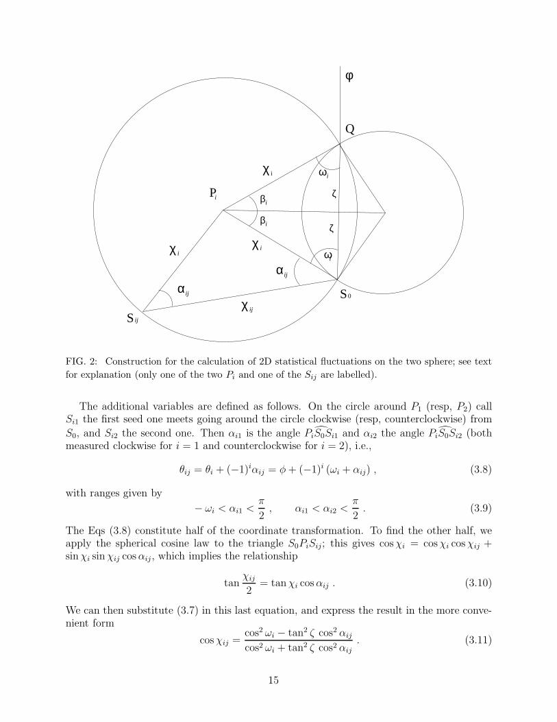
ij

S

χ

χ

ζ

ζ

χ

χS

β

β

i

P

i

0

ij

i

i

i

i

iω

ωi

Q

φ

ij

ijαα

FIG. 2: Construction for the calculation of 2D statistical fluctuations on the two sphere; see text

for explanation (only one of the two Pi and one of the Sij are labelled).

The additional variables are defined as follows. On the circle around P1 (resp, P2) callSi1 the first seed one meets going around the circle clockwise (resp, counterclockwise) from

S0, and Si2 the second one. Then αi1 is the angle PiS0Si1 and αi2 the angle PiS0Si2 (bothmeasured clockwise for i = 1 and counterclockwise for i = 2), i.e.,

θij = θi + (−1)iαij = φ + (−1)i (ωi + αij) , (3.8)

with ranges given by

− ωi < αi1 <π

2, αi1 < αi2 <

π

2. (3.9)

The Eqs (3.8) constitute half of the coordinate transformation. To find the other half, weapply the spherical cosine law to the triangle S0PiSij; this gives cos χi = cos χi cos χij +sin χi sin χij cos αij , which implies the relationship

tanχij

2= tan χi cos αij . (3.10)

We can then substitute (3.7) in this last equation, and express the result in the more conve-nient form

cos χij =cos2 ωi − tan2 ζ cos2 αij

cos2 ωi + tan2 ζ cos2 αij

. (3.11)

15

With (3.8) and (3.11) we can now rewrite the full measure of integration (3.4) in terms ofthe new variables. After a somewhat lengthy calculation, one obtains

dµ1 dµ2 = dζ dφ dω1 dω2 dα11 dα12 dα21 dα22

× 256 ρ4a8 tan7 ζ (1 + tan2 ζ)

∏

i,j=1,2

cos αij

(cos2 ωi + tan2 ζ cos2 αij)2

×

× cos3 ω1 cos3 ω2 sin(ω1 + ω2) sin(α22 − α21) sin(α12 − α11) . (3.12)

We now need to calculate the area A(V1 ∪V2) of the union of the disks around P1 and P2.The line S0Q divides each of the Vi into two parts, and V1 ∪ V2 is the disjoint union of onepart from each Vi (see figure) which, for the purpose of finding its area, it is convenient tothink of as Vi with the “wedge” S0PiQ removed and replaced by the triangle S0PiQ. Thuswe can write

A(V1 ∪ V2) =∑2

i=1(Adisk − Awedge + Atriangle)i =

∑2

i=1[π + 2ω − (π − β) cosχ] a2 , (3.13)

where some simple spherical geometry gives

Adisk i = 2π (1 − cos χi) a2

Awedge i = 2βi (1 − cos χi) a2

Atriangle i = 2 (βi + ωi − 12π) a2 . (3.14)

Here, βi is half of the internal angle of the wedge or the triangle S0PiQ at Pi. Using the sinelaw with half the triangle QS0Pi, we obtain that it is related to our variables by

cos βi = cos ζ sin ωi , (3.15)

and we obtain from (3.7) that

cos2 χi =cos2 ωi

cos2 ωi + tan2 ζ. (3.16)

Putting these pieces together we therefore have

A(V1 ∪ V2) = a22∑

i=1

π + 2 ωi −

2 cosωi√cos2 ωi + tan2 ζ

(π − arccos(cos ζ sin ωi))

, (3.17)

and the expectation value we are looking for is obtained integrating the product of theseprobabilities over all locations of the four seeds,

N0,0′ =∫

dµ1

∫dµ2 e−ρ A(V1∪V2) , (3.18)

Finally, substituting this in the expression for the variance of N0, we get

σ21 = 2 N0,0′ + 3 N1 − N1

2= 2

∫dµ1

∫dµ2 e−ρ A(V1∪V2) − 18

(1 − 3

4π

R

ρ+

1

8π2

R2

ρ2

). (3.19)

16

This integral can be evaluated numerically for any given value of ρ/R.We are now in a position to discuss the geometries we associate with a 2-dimensional

Voronoi complex Ω. Since in two dimensions the curvature is completely characterized bythe Ricci scalar R, our goal is to associate a value of R, with suitable uncertainties, withevery set U in a cover of a manifold M ≃ Ω that is made of sufficiently small sets. Westart by selecting a larger collection of candidate sets, and then explain how to pick theappropriate ones among them. For each 2-cell ω0 ∈ Ω consider the family of sets Uω0,λ,λ = 0, 1, 2, ..., defined by

Uω0,0 = ω0, Uω0,λ+1 = Uω0,λ ∪ ω ∈ Ω | ∂ω ∩ ∂Uω0,λ 6= ∅ ; (3.20)

in other words, Uω0,λ is ω0 together with the first λ layers of neighboring 2-cells around it.Roughly speaking, if we call Nω0,λ the number of 2-cells in Uω0,λ, in an approximately flat2-geometry we expect to have Nω0,λ ≈ 1 + 6 + 12+ ... + 6λ = 3λ2 + 3λ + 1. A value of R canbe assigned to each ω0 simply by using (3.2) as an estimate,

R(ω0) = 4πρ(1 − 1

6N1(ω0)

). (3.21)

This value however is not a good one as far as manifold geometry goes; differences betweenit and those obtained for neighboring 2-cells should be interpreted not as real variations of Rbut as statistical fluctuations. What we should do instead is average the values obtained fora cluster of neighboring 2-cells, i.e., a suitably large Uω0,λ. If we knew that the continuumgeometry will turn out to be a constant curvature one, the best strategy would be to pickλ as large as possible, in order to maximize the statistics. In practice, if we use too many2-cells we may be combining regions that in a good fit of the geometry would have differentcurvatures, so we need to specify a procedure for picking an optimal λ. Pick some value ofλ. Then, at scale λ, Uω0,λ provides a sample of size Nω0,λ from the ensemble of all 2-cellsin a manifold of assumed constant curvature, and our best estimate for the scalar curvaturearound ω0 is the average

R(Uω0,λ) = 〈R(ω)〉ω∈Uω0,λ= 4πρ

(1 − 1

6〈N1(ω)〉ω∈Uω0,λ

), (3.22)

with the variance in the distribution of averages over such samples being given by

σ2〈N1〉

= N−1ω0,λ σ2

1 . (3.23)

If this variance is small, we can use it to estimate a range of values of R which would haveproduced values of 〈N1(ω)〉 within this tolerance, by setting ∆R = (dR/d〈N1〉) σ〈N1〉, or

∆R(Uω0,λ) =2πρ

3σ〈N1〉 =

2πρ

3N

−1/2ω0,λ σ1 . (3.24)

Finally, the whole process is self-consistent and gives a good continuum approximation toΩ if differences between the scalar curvatures estimated from neighboring regions Uω0,λ aresmaller than the statistical uncertainty ∆R(Uω0,λ) within individual regions, i.e., R is slowlyvarying on the scales given by λ.

17

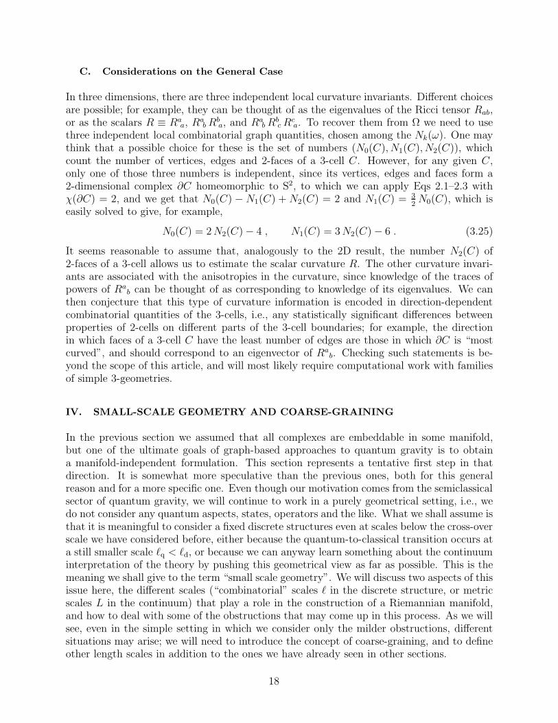
C. Considerations on the General Case

In three dimensions, there are three independent local curvature invariants. Different choicesare possible; for example, they can be thought of as the eigenvalues of the Ricci tensor Rab,or as the scalars R ≡ Ra

a, Rab Rb

a, and Rab Rb

c Rca. To recover them from Ω we need to use

three independent local combinatorial graph quantities, chosen among the Nk(ω). One maythink that a possible choice for these is the set of numbers (N0(C), N1(C), N2(C)), whichcount the number of vertices, edges and 2-faces of a 3-cell C. However, for any given C,only one of those three numbers is independent, since its vertices, edges and faces form a2-dimensional complex ∂C homeomorphic to S2, to which we can apply Eqs 2.1–2.3 withχ(∂C) = 2, and we get that N0(C) − N1(C) + N2(C) = 2 and N1(C) = 3

2N0(C), which is

easily solved to give, for example,

N0(C) = 2 N2(C) − 4 , N1(C) = 3 N2(C) − 6 . (3.25)

It seems reasonable to assume that, analogously to the 2D result, the number N2(C) of2-faces of a 3-cell allows us to estimate the scalar curvature R. The other curvature invari-ants are associated with the anisotropies in the curvature, since knowledge of the traces ofpowers of Ra

b can be thought of as corresponding to knowledge of its eigenvalues. We canthen conjecture that this type of curvature information is encoded in direction-dependentcombinatorial quantities of the 3-cells, i.e., any statistically significant differences betweenproperties of 2-cells on different parts of the 3-cell boundaries; for example, the directionin which faces of a 3-cell C have the least number of edges are those in which ∂C is “mostcurved”, and should correspond to an eigenvector of Ra

b. Checking such statements is be-yond the scope of this article, and will most likely require computational work with familiesof simple 3-geometries.

IV. SMALL-SCALE GEOMETRY AND COARSE-GRAINING

In the previous section we assumed that all complexes are embeddable in some manifold,but one of the ultimate goals of graph-based approaches to quantum gravity is to obtaina manifold-independent formulation. This section represents a tentative first step in thatdirection. It is somewhat more speculative than the previous ones, both for this generalreason and for a more specific one. Even though our motivation comes from the semiclassicalsector of quantum gravity, we will continue to work in a purely geometrical setting, i.e., wedo not consider any quantum aspects, states, operators and the like. What we shall assume isthat it is meaningful to consider a fixed discrete structures even at scales below the cross-overscale we have considered before, either because the quantum-to-classical transition occurs ata still smaller scale ℓq < ℓd, or because we can anyway learn something about the continuuminterpretation of the theory by pushing this geometrical view as far as possible. This is themeaning we shall give to the term “small scale geometry”. We will discuss two aspects of thisissue here, the different scales (“combinatorial” scales ℓ in the discrete structure, or metricscales L in the continuum) that play a role in the construction of a Riemannian manifold,and how to deal with some of the obstructions that may come up in this process. As we willsee, even in the simple setting in which we consider only the milder obstructions, differentsituations may arise; we will need to introduce the concept of coarse-graining, and to defineother length scales in addition to the ones we have already seen in other sections.

18

A. Length Scales

One general issue that needs to be addressed is that of identifying the various length scalesthat appear in our framework, and assigning dimensional values to combinatorial quantitiesin Ω. Since we are assuming that the fundamental theory is formulated in terms of Ω, wewould want to describe those length scales using quantities intrinsic to Ω, and be able tomake statements such as “at scale ℓq, Ω cannot be embedded in a manifold,” which impliesthat a continuum geometry is not available to provide a meaning for length scales.

Continuum theories include a number of length scales associated with various phenomena;results of measurements are interpreted in terms of those scales and provide values for them,so in order to provide values for scales intrinsic to Ω it is natural to go through a correspon-dence with continuum length scales. An obvious one to try to identify in terms of Ω is thePlanck length LP (when Ω is dressed with other variables it may be possible to do this evenat the kinematical level, as in the case of the calculation of the loop spacing for the heuristicweave states in loop quantum gravity [18]), but any prediction of the discrete theory thathas a continuum counterpart can be used, and when more than one will be available thediscrete theory can be tested.

A discrete structure of the type we are discussing also provides various scales. For example,if we start with a Voronoi cell complex, we can embed it in a geometry that has no lengthscales smaller than the cell size. The latter cannot be assigned a dimensional value yet,because the situation is invariant under a global rescaling of the metric, but we will saythat Ω is associated with a semiclassical cross-over scale ℓs equal to its discreteness scaleℓd. If we start with a D-dimensional Voronoi complex Ω that is not a cell complex, butis such that we can obtain a cell complex Ω′ by coarse-graining Ω and removing a fraction0 < ξ < 1 of its D-dimensional tiles, we will say that Ω′ corresponds to the semiclassicalscale ℓs, at which it and its dual Ω′∗ represent the manifold well, while Ω is characterized bythe discreteness scale ℓd = (1 − ξ)1/Dℓs. In either case, it may not be possible to determinethe metric or curvature of the geometry at scale ℓs, because at that scale we do not haveenough statistics to reliably use the techniques we will describe. Instead, the classical scaleℓc is the linear size, in terms of number of cells, of the regions in Ω used as approximationsto the manifold regions X such that the continuum geometry can be determined with smallstatistical fluctuations. That geometry itself, possibly together with the global topology ofM, may also determine larger length scales ℓg (both local ones defined by the curvatureand its rate of change or higher derivatives, and possibly global ones defined for example bynon-trivial homotopy generators).

Summarizing, the length scales ℓd ≤ ℓs ≤ ℓc ≤ ℓg are determined by the structure of Ω, ifΩ is a discrete structure of a type that allows us to define ℓs, given a suitable definition of acoarse-graining procedure. In quantum gravity, we will then require, as part of the definitionof a semiclassical state, the condition that Ψ be associated with a discrete structure forwhich ℓs exists. On the other hand, continuum-based physics determines a length scaleLP for quantum gravity, given in terms of fundamental physical constants by dimensionalarguments and back-of-the-envelope calculations of quantum gravity fluctuations [2], whichappears also in the eigenvalues of the quantum geometry operators for areas and volumes; Itis not clear to us whether this scale should be identified with ℓd or ℓc, if different, or how thisrelationship might be affected by renormalization arguments. Finally, physics also determinesa phenomenological, “macroscopic” scale Lm ≫ LP, which depends on the experimental

19

techniques used but that can be assumed to be larger than ℓs. A good understanding of therelationships between all of these scales is outside the scope of this paper, but our discussionof coarse-graining will be a start in this direction.

B. Coarse-Graining

Some complexes Ω can be directly associated with a “macroscopic” geometry, in the sensethat they can be embedded homeomorphically in a manifold at a length scale ℓc and theprocedures previously described give a well-defined (approximate) geometry at a length scaleℓs, in which case the “semiclassical” interpretation is relatively straightforward, within theappropriate statistical uncertainties. That is, Ω gives us a classical, mesoscopic geometry.At larger scales, for which the number of points to be taken per sample cell is larger, oneexpects a very good approximation, according to our own set of conditions. The remainingquestion then is: What if Ω does not satisfy the requirements for approximating a nicegeometry? Although there then is no direct association between graph and geometry, ifin an appropriate sense the obstructions only occur on small scales, it may be possible tocoarse-grain the graph to a larger-scale one that is associated with a continuum geometry.

The coarse-graining procedure will be one which, intuitively, takes a graph Ω at a certainscale and maps it to a different, larger-scale Ω′. There are two possibilities on how to performthe coarse graining in this case. The first possibility, that we call soft coarse-graining, hasthe following strategy: One assumes that one has a Voronoi or Delaunay complex and onegets to a coarser one by “ignoring” the structure below a certain scale simply by averagingthe quantities of interest over neighboring cells. This is what we have already done in Sec IIIwhen looking for the optimal mesoscopic scale at which to define slowly varying quantities;we are not actually defining a new complex, and it can always be done. In the secondpossibility, that we will refer to as hard coarse-graining, we have a procedure that connectstwo graphs, and one gets the larger graph Ω′ by removing cells (Delaunay vertices) from Ω,in a precise way.

Hard coarse graining, which implies a modification of the underlying graph, represents anew input in our considerations. This procedure is achieved by a sequence of cellular moves

that refine the cellular decomposition [19]. These moves have been shown to provide a pre-scription for refining and coarsening the complex (they are in a sense more elementary thanthe Pachner moves). The intuitive idea for the coarse graining is that two adjacent n-cells ofthe complex that share an (n− 1)-cell get ‘fused’ into a new n-cell. This refining/coarseningprocedure has already been used for defining renormalization prescriptions in discrete sys-tems [20], and the approximation to smooth manifolds by our proposed hard coarse-grainingis an explicit example of some of those prescriptions.

In order to have a proper understanding of the different scenarios that one might en-counter given an arbitrary graph at small scales, with the purpose of incorporating it intoour geometrical formalism, let us make the following classification in decreasing order of‘complexity’:

1. In the most exotic scenario one starts with a Voronoi complex that does not have a dualcell complex. This means that there is no dual triangulation and the correspondinggraph might be disconnected. Since this happens for cases where, say, one sprinkles

20

points in a manifold with a density that is “too low”, and no real statistics is possible,we will exclude this case from our considerations here.

2. The next possibility is that the given cell complex Ω can not be embedded into anymanifold M. This means that the complex is not topologically a cell decomposition ofa manifold. In this case one might hope that with a proper coarse graining one mightbe able to take this complex to a new one Ω′ that does admit such interpretation andcan be embedded. Physically, one could say that the original complex represented aspace that on certain small scales has ‘topological’ and/or ‘dimensional’ fluctuations.This is the trickiest situation where one needs a ‘hard coarse graining’, for which weare not aware of an existing specific procedure, and it is certainly a question worthpursuing.

3. A milder scenario is to consider as the starting point a cell complex Ω that is a celldecomposition of a manifold M but that is not Voronoi, in the sense that the valenceof the graph is not equal to D + 1. In this scenario, one would allow for “fluctuatingvalence” in the Voronoi cell, but with average 〈N1|0〉 = 4, in 3D. This means thatthe graph that defines the quantum state at Planck scale does not have the ‘Voronoisignature’, which might be the case for an arbitrary graph in loop quantum gravity.In this case we can implement the cell moves of Ref [19] to turn it into a Voronoicell complex; if the authors’ conjecture is correct, via these cellular moves one canalways transform any cell decomposition into a Voronoi one, that will serve as startingpoint for the statistical geometry considerations described in previous sections. Oneshould also note that in some cases this ‘restructuring’ of the cell complex might notcorrespond to a course graining in the strict sense, since the moves that ‘lower’ thevalence of the Voronoi graph do not remove cell complexes to it as one might expectfrom a coarse graining procedure.

In the next, final section we shall consider quantum issues and relate the formalisms wehave been employing to the task of bridging the gap between a semiclassical state in loopquantum gravity and classical geometry.

V. PLANCK SCALE GEOMETRY AND BEYOND

In this section we make precise the connection between the previous sections and semiclas-sical canonical quantum gravity, i.e., the low energy limit of loop quantum gravity. Thissection has two parts. In the first one, we outline how one can try to use our framework tocomplement present approaches to semi-classical states in LQG. In the second part we outlinethe steps to be followed in order to estimate statistical errors in making phenomenologicalpredictions out of the semiclassical states.

A. Semiclassical States

In order to deal with the low energy limit of the theory, we will again have to deal with thefact that there might be new length scales in the description of the quantum geometry. So

21

far we have considered in great detail the way in which we may approximate a macroscopicgeometry starting from a graph or complex at a much smaller scale. Even though we haveintroduced a microscopic discrete scale ℓd, at which the finest graph might be defined, thisscale is not necessarily related to a particular quantum scale ℓq. As discussed in Sec II, thereare standard dimensional arguments which indicate that the relevant scale ℓq for a quantumstate is the Planck length LP. This only means that the quantum excitations of the geometry,which could be elements of area through edges of the graph or contributions to the volumefrom the vertices, yield eigenvalues of the order of the Planck scale for single edges/vertices(at least for the unrenormalized value of the Barbero-Immirzi parameter γ of order one thatis used nowadays). Whenever we consider a semiclassical state Ψsc in loop quantum gravity,there are several steps and assumptions involved in estimating the continuum geometry itcorresponds to. Let us now explore what those assumptions are.

The first assumption is that the true nature of geometry at the Planck length is describedby loop quantum geometry. Second, we assume that we can define certain states (Coherent[24], Shadow [15], Gaussian [26], etc.) that will be semiclassical in the sense of approximatinga geometry (and its time derivative), in the ‘correct phase’. Finally, one is assuming thata definite picture of the quantum geometry will emerge from a precise merger of both loopquantum gravity and our “discrete-statistical” approach. In this viewpoint, the final picturelooks like this: The ‘true state’ is given by a properly defined state in loop quantum gravity,featuring quantum behavior at the Planck scale. The graph that we use to define this ‘shadowstate’ (to give an example) will be a Voronoi graph. The semiclassical state will have theproperty that, when probed on a mesoscopic scale ℓc (still to be specified in practice) itwill behave quasi-classically (hopefully, with respect the the coarse-grained operators thatwe need to define). This means that in order to construct the desired semiclassical statefollowing the steps of Ref [21], the operators that we specify as belonging to the set to beapproximated (together with the tolerances) will not be operators assigned to observablesat the quantum, Planck scale.

We are interested in constructing states that approximate quantities at a scale ℓs, wherethe quantum-classical transition takes place. As already mentioned, this new scale, yet to beidentified, could be assumed to be close to the mesoscopic scale ℓc, but it should be smaller.Going to our analogy model of fluids, the transition quantum-classical can be assumed totake place at a smaller scale than the one at which averages are taken and the continuumapproximation emerges (for the simple reason that one adds velocities of particles containedin the region, which already presupposes classical attributes for the constituents of the fluid).The viewpoint that new, mesoscopic scales have to be considered has already been exploredby other authors who have explored the semiclassical limit before [25].

The next question we would like to address is the possible utility of our statistical methodsfor distinguishing between good and bad candidates for semiclassical states. That is, supposethat we are given an alleged semiclassical state Ψsc and we are assigned the task of testingit. The strategy for doing so is the following. Compute expectation values and fluctuationsfor the cell-based, observables that the maker of the state claims it approximates well. Makesure that the state is defined on a Voronoi complex. Dress the complex with the expectationvalues found for the observables. Now the crucial step is to compare this dressing with thegeometry we expect to get from the complex itself, as in Sec III, and verify that they areconsistent. If they are not, return the state to the maker.

22

B. Phenomenology

Suppose now that the given state satisfies all criteria set by some considerations, then inour procedure we would have to pass it to the next step in the testing line: see whether itfits observations. Now this is a very intricate question, for we have not specified the phe-nomenological criteria that a semiclassical state should satisfy, nor the expected observabledeviations from the classical realm (Lorentz violation, modified dispersion relations, non-commutativity, birefringence, etc) [27]. Note also that this procedure implies the knowledgeof more quantities assigned to the cell complex, more than what we have up to now specifiedin the complex. This further ‘dressing of the complex’ will be dealt with in a forthcomingpaper [8].

What we could attempt to answer is the following simpler question. Suppose that weexpect the state to approximate the geometry gab. As we have discussed before, there arenow two sources of uncertainty in the approximation of this spacetime geometry (even thoughwe were working in the canonical picture, we can talk about a spacetime geometry). Thefirst source is a well known one, due to quantum fluctuations: observables OI that werechosen to be approximated by the state have quantum dispersions (∆OI)Ψ. The secondsource of uncertainty is the statistical nature of our reconstruction procedure. That is, aswe have argued before, the macroscopic continuous geometry is only a fiction, very usefulfor describing phenomena at certain scales, but it is only an approximation to the truegeometry. But there is not a unique macroscopic metric that can be approximated by thegraph: rather, there is an ‘ensemble’ of such metrics, which then introduces a classicalor cross-over uncertainty (∆OI)c in the observables. The observational imprint that thisuncertainty might bring is manifested by the fact that we normally use a fiducial classicalmetric to perform geometrical measurements. We expect that this geometry belongs to theset of possible geometries that are approximated by the graph, but it might turn out tobe not the ‘most probable’ one, and thus one might be introducing an extra error in ourinterpretation of the experimental results. Note that these errors are of a different naturethan those that arise from the use of a regular lattice in [10]. We expect that we won’t havethese ‘discretization errors’ due to the use of the Voronoi construction. In order to havefull control over the different sources of uncertainty, one would like to quantify them anddecide which one is the dominant one. At this point we are not in the position of having aworking hypothesis for this question, and we can only make an educated guess as to the wayin which the two uncertainties interact with each other. Under the most naive assumptionof independence, one might say that the total uncertainty is

(∆OI)2t = (∆OI)

2Ψ + (∆OI)

2c .

An important issue is to quantify the fluctuations that can be attributed to both effects, andknow how the total fluctuation for each observable depends on them, since we would like tobe able to subtract any statistical ‘spurious’ information and be able to measure the purequantum contributions to the problem.

Assuming that the semiclassical state had these desired properties —an issue that liesoutside the scope of this paper— would lead us to conclude, from a strict viewpoint thatwe have succeeded in our task of constructing a semiclassical geometry. This is becausethis state should then approximate any observations, at the mesoscopic level that we shallperform on the geometry (with external matter) and thus, if we now take the viewpoint thatit is enough to describe what we can observe, we would reach our conclusion.

23

C. Summary and Outlook

To summarize, we have introduced a framework for establishing a bridge between the de-scription of geometry of space in terms of semiclassical states for quantum gravity, and theone used in phenomenological calculations of corrections to field theory in curved space. Atthe most basic level, our proposal fits in with the general idea that the type of discretenessone encounters in a class of approaches to quantum gravity implies that the amount of infor-mation contained in a finite spacetime volume is finite, which has been explored in a varietyof contexts [28]. Our work then suggests a specific way to translate this idea into quantitativeexpressions for the information a discrete structure contains about a continuum geometry,using statistical geometry. To illustrate how the framework is used, we have characterizeda semiclassical quantum gravity state by a single cell complex and a single set of valuesfor variables motivated by loop quantum gravity. Such a characterization, of course, is notintended to be complete; it might arise as part of the specification of a coherent state [24],or from a “shadow state” used to probe Ψsc [15], but for our purposes it is just a tool thatallows us to isolate the statistical effects we want to study. It is a tool that complements thecriteria one might have in choosing the quantum state.

The general picture that emerged in this framework is one in which, from a certain lengthscale upward, if the quantities characterizing the state are sufficiently regular, the mesoscopicgeometry is determined up to quantifiable uncertainties. Once those uncertainties will bebetter understood, especially in three dimensions, one can begin to look into the possibilityof adding matter coupled to gravity, and how these uncertainties need to be combined withquantum fluctuations to give measurable effects on observable quantities. The answer to thislast question will probably depend on which observations are carried out, and it is in principlepossible that one can use observable effects that depend only on quantum uncertainties;after all, going back to the gas analogy, when we want to study the quantum properties ofatoms, we do not need to combine their quantum fluctuations with the statistical mechanicsdescription of a gas. But a gas is different, and we do not need to have information aboutthe state of the whole gas to even be able to describe what each atom does.

In this paper we have concentrated our attention to graphs that did not have any othergeometrical information other than what is already in its definition. In order to have an ap-proach closer to the variables used in LQG one would like to have assigned certain (classical)quantities to the graph Ω, that is, one would like to consider ‘dressed’ graphs. This will bedealt with in a subsequent publication [8].

Acknowledgements

LB and AC would like to thank Perimeter Institute for hospitality. Partial support for thiswork was provided by NSF grant PHY-0010061, CONACyT grant J32754-E andDGAPA-UNAM grant 112401.

[1] C Rovelli 2001 “Quantum space-time: What do we know?” in C Callender (ed) Physics

Meets Philosophy at the Planck Scale 101–122, arXiv:gr-qc/9903045; C Rovelli 2000 “The

24

century of the incomplete revolution: Searching for general relativistic quantum field theory,”

J. Math. Phys. 41 3776, arXiv:hep-th/9910131.

[2] J A Wheeler 1962 Geometrodynamics Academic Press.

[3] A Ashtekar and J Lewandowski 2004 “Background independent quantum gravity: A status

report,” arXiv:gr-qc/0404018; C Rovelli “Quantum Gravity”, (Cambridge U. Press, 2004);

C Rovelli 1998 “Loop quantum gravity,” Living Rev. Rel. 1 1 arXiv:gr-qc/9710008; T

Thiemann 2001 “Introduction to modern canonical quantum general relativity,”

arXiv:gr-qc/0110034.

[4] R M Williams and P A Tuckey 1992 “Regge calculus: A Bibliography and brief review,”

Class. Quantum Grav. 9 1409; T Regge and R M Williams 2000 “Discrete structures in

gravity,” J. Math. Phys. 41 3964, arXiv:gr-qc/0012035.

[5] R Loll 1998 “Discrete approaches to quantum gravity in four dimensions,” Living Rev. Rel. 1

13, arXiv:gr-qc/9805049.

[6] A Perez 2003 “Spin foam models for quantum gravity,” Class. Quantum Grav. 20 R43,

arXiv:gr-qc/0301113; D Oriti 2003 “Spin foam models of quantum spacetime,”

arXiv:gr-qc/0311066.

[7] L Bombelli, J Lee, D Meyer and R D Sorkin 1987 “Space-time as a causal set” Phys. Rev.

Lett. 59 521–524; R D Sorkin 2003 “Causal sets: Discrete gravity (Notes for the Valdivia

Summer School),” arXiv:gr-qc/0309009.

[8] L Bombelli, A Corichi and O Winkler 2004 in preparation.

[9] N H Christ, R Friedberg and T D Lee 1982 “Random lattice field theory: General

formulation” Nucl. Phys. B202 89–125; T D Lee 1985 “Discrete mechanics”, in A Zichichi, ed

How Far Are We from the Gauge Forces (XXI Ettore Majorana School, Erice 1983) Plenum.

[10] H Sahlmann and T Thiemann 2002 “Towards the QFT on curved spacetime limit of QGR. I:

A general scheme,” arXiv:gr-qc/0207030; H Sahlmann and T Thiemann 2002 “Towards

the QFT on curved spacetime limit of QGR. II: A concrete implementation,”

arXiv:gr-qc/0207031;

[11] A Ashtekar and J Lewandowski 1997 “Quantum theory of geometry. II: Volume operators”

Adv. Theor. Math. Phys. 1 388–429, gr-qc/9711031.

[12] L Santalo 1976 Integral Geometry and Geometric Probability Addison Wesley.

[13] C Itzykson & J M Drouffe 1989 Statistical Field Theory Cambridge University Press.

[14] L Bombelli 2002 “Statistical geometry of random weave states” Proceedings of the Ninth

Marcel Grossmann Meeting on General Relativity, eds V G Gurzadyan, R T Jantzen and R

Ruffini, World Scientific, arXiv:gr-qc/0101080.

[15] A Ashtekar and J Lewandowski, 2001 “Relation between polymer and Fock excitations,”

Class. Quantum Grav. 18 L117, arXiv:gr-qc/0107043.

[16] L Bombelli 2000 “Statistical Lorentzian geometry and the closeness of Lorentzian manifolds”

J. Math. Phys. 41 6944–6958, arXiv:gr-qc/0002053

[17] K Brakke 1985 “Statistics of random plane Voronoi tessellations,” preprint.

[18] A Ashtekar, C Rovelli and L Smolin 1992 “Weaving a classical geometry with quantum

threads,” Phys. Rev. Lett. 69 237 arXiv:hep-th/9203079; N Grot and C Rovelli 1997

“Weave states in loop quantum gravity,” Gen. Rel. Grav. 29 1039.

[19] F Girelli, R Oeckl and A Perez 2002 “Spin foam diagrammatics and topological invariance”

Class. Quant. Grav. 19, 1093 arXiv:gr-qc/0111022

[20] R Oeckl 2003 “Renormalization of discrete models without background,” Nucl. Phys. B657

25

107, arXiv:gr-qc/0212047; R Oeckl 2004 “Renormalization for spin foam models of

quantum gravity,” arXiv:gr-qc/0401087; F Markopoulou 2003 “Coarse graining in spin

foam models,” Class. Quantum Grav. 20 777, arXiv:gr-qc/0203036.

[21] A Ashtekar, L Bombelli and A Corichi 2004 “Coherent and semiclassical states for

constrained systems,” in preparation.

[22] W A Miller 1997 “The Hilbert action in Regge calculus” Class. Quantum Grav. 14

L199–L204, arXiv:gr-qc/9708011.

[23] A Okabe et al 1999 Spatial Tessellations 2nd ed, Wiley.

[24] H Sahlmann, T Thiemann and O Winkler, 2001 “Coherent states for canonical quantum

general relativity and the infinite tensor product extension,” Nucl. Phys. B 606 401.

arXiv:gr-qc/0102038.

[25] M Bojowald and H A Morales-Tecotl 2003 “Cosmological applications of loop quantum

gravity,” arXiv:gr-qc/0306008; J Alfaro, H A Morales-Tecotl and L F Urrutia 2002 “Loop

quantum gravity and light propagation,” Phys. Rev. D 65: 103509, arXiv:hep-th/0108061;

J Alfaro and G Palma 2003 “Loop quantum gravity and ultra high energy cosmic rays,”

Phys. Rev. D 67: 083003, arXiv:hep-th/0208193; J Alfaro, H A Morales-Tecotl and L F

Urrutia 2002 “Quantum gravity and spin-12 particles effective dynamics,” Phys. Rev. D 66:

124006, arXiv:hep-th/0208192;

[26] A Corichi and J M Reyes 2001 “A Gaussian weave for kinematical loop quantum gravity,”

Int. J. Mod. Phys. D 10 325, arXiv:gr-qc/0006067.

[27] T Jacobson, S Liberati and D Mattingly 2004 “Quantum Gravity Phenomenology and

Lorentz violation,” arXiv:gr-qc/0404067; G Amelino-Camelia 2004 “Some encouraging and

some cautionary remarks on doubly special relativity in quantum gravity,”

arXiv:gr-qc/0402092; R C Myers and M Pospelov 2004 “Experimental challenges for

quantum gravity,” arXiv:gr-qc/0402028; J Collins, A Perez, D Sudarsky, L Urrutia and H

Vucetich 2004 “Lorentz invariance: An additional fine-tuning problem,”

arXiv:gr-qc/0403053.

[28] See, e.g., A Kempf 2003 “A covariant information-density cutoff in curved space-time”

arXiv:gr-qc/0310035.

26