Dynamics of continuous-time quantum walks in restricted geometries

arX

iv:0

810.

1184

v1 [

quan

t-ph

] 7

Oct

200

8

Dynamics of continuous-time quantum walks in

restricted geometries

E. Agliari, A. Blumen and O. Mulken

Theoretische Polymerphysik, Universitat Freiburg, Hermann-Herder-Str. 3, D-79104

Freiburg, Germany

Abstract. We study quantum transport on finite discrete structures and we model

the process by means of continuous-time quantum walks. A direct and effective

comparison between quantum and classical walks can be attained based on the average

displacement of the walker as a function of time. Indeed, a fast growth of the average

displacement can be advantageously exploited to build up efficient search algorithms.

By means of analytical and numerical investigations, we show that the finiteness and

the inhomogeneity of the substrate jointly weaken the quantum walk performance. We

further highlight the interplay between the quantum-walk dynamics and the underlying

topology by studying the temporal evolution of the transfer probability distribution

and the lower bound of long time averages.

PACS numbers: 05.60Gg, 71.35.-y, 05.60Cd

http://arXiv.org/abs/0810.1184v1

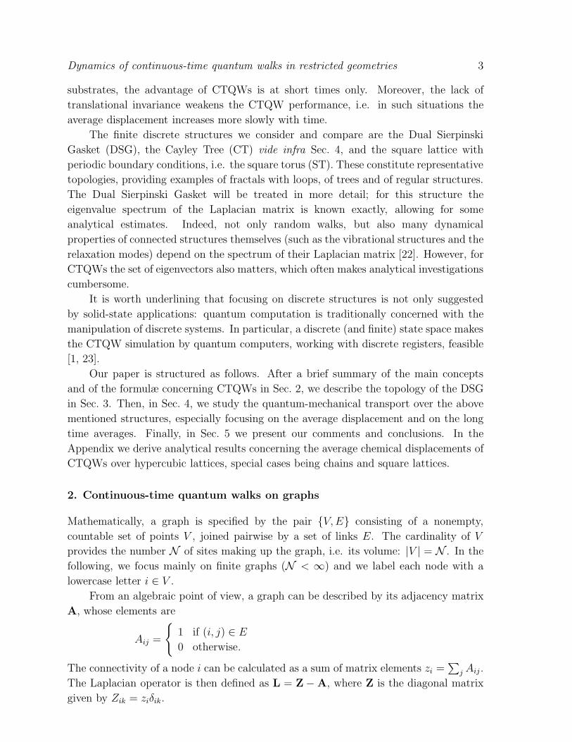
Dynamics of continuous-time quantum walks in restricted geometries 2

1. Introduction

Quantum walks (QWs) are attracting increasing attention in many research areas,

ranging from solid-state physics to quantum computing [1]. In particular, QWs provide a

model for quantum-mechanical transport processes on discrete structures; this includes,

for instance, the coherent energy transfer of a qubit on an optical lattice [2, 3, 4, 5]. The

theoretical study of QWs is also encouraged by recent experimental implementations

able to corroborate theoretical findings [6, 7, 8].

As in the classical random walk, quantum walks appear in a discrete [9] as in a

continuous-time (CTQW) [10] form; these forms, however, cannot be simply related

to each other [11]. Now, standard CTQWs, on which we focus, can be obtained by

identifying the Hamiltonian of the system with the classical transfer matrix which is, in

turn, directly related to the Laplacian of the underlying structure.

Another feature which CTQWs share with classical random walks consists in the

strong interplay between the dynamics properties displayed by the walk and the topology

of the substrate [12, 13, 14]. However, the dependencies turn out to be much more

complex in the quantum-mechanical case: while the classical (simple) walk eventually

loses memory of its starting site, the quantum walk exhibits, even in the asymptotic

regime, transition probabilities which depend on the starting site. For this reason, often

the parameters describing the transport are averaged over all initial sites, a procedure

which allows a global characterization of the walk, while preserving its most important

features.

One of the quantities affected by topology is the mean square displacement of the

walker up to time t. Classically, this quantity is monotonically increasing and depends

(asymptotically) on time according to the power law 〈r2(t)〉 ∼ tβ. The value of the

“diffusion exponent” β allows to distinguish between normal (β = 1) and anomalous

(β 6= 1) diffusion [15]. As for quantum transport, it is possible to introduce analogous

exponents, characterizing the temporal spreading of a wave-packet [16]. However, even

when they take place over the same structure, quantum and classical walks can exhibit

dramatically different behaviours. In particular, the quantum wave propagation on

regular, infinite lattices is ballistic, i.e. the root mean square displacement is linear

in time. Such a quadratic speed-up of the mean square displacement is a well known

phenomenon when dealing with tight-binding electron waves on periodic lattices [9]

and, from a computational point of view, it constitutes an important feature since it

could be advantageously exploited in quantum search algorithms [17, 18, 19]. In the

presence of disorder (either deterministic or stochastic) or finiteness, the sharp ballistic

fronts are softened, a fact which may even lead to the localization of the quantum

particle [20, 21]. It is therefore of both theoretical and practical interest to highlight how

finiteness and inhomogeneity - often unavoidable in real systems - affect the particle’s

propagation. To this aim we analyze quantum transport on restricted geometries, where

the restrictions arise from the (possibly joint) fractal dimension and finite extent of the

substrate itself. By direct comparison with the classical case, we find that, on finite


substrates, the advantage of CTQWs is at short times only. Moreover, the lack of

translational invariance weakens the CTQW performance, i.e. in such situations the

average displacement increases more slowly with time.

The finite discrete structures we consider and compare are the Dual Sierpinski

Gasket (DSG), the Cayley Tree (CT) vide infra Sec. 4, and the square lattice with

periodic boundary conditions, i.e. the square torus (ST). These constitute representative

topologies, providing examples of fractals with loops, of trees and of regular structures.

The Dual Sierpinski Gasket will be treated in more detail; for this structure the

eigenvalue spectrum of the Laplacian matrix is known exactly, allowing for some

analytical estimates. Indeed, not only random walks, but also many dynamical

properties of connected structures themselves (such as the vibrational structures and the

relaxation modes) depend on the spectrum of their Laplacian matrix [22]. However, for

CTQWs the set of eigenvectors also matters, which often makes analytical investigations

cumbersome.

It is worth underlining that focusing on discrete structures is not only suggested

by solid-state applications: quantum computation is traditionally concerned with the

manipulation of discrete systems. In particular, a discrete (and finite) state space makes

the CTQW simulation by quantum computers, working with discrete registers, feasible

[1, 23].

Our paper is structured as follows. After a brief summary of the main concepts

and of the formulæ concerning CTQWs in Sec. 2, we describe the topology of the DSG

in Sec. 3. Then, in Sec. 4, we study the quantum-mechanical transport over the above

mentioned structures, especially focusing on the average displacement and on the long

time averages. Finally, in Sec. 5 we present our comments and conclusions. In the

Appendix we derive analytical results concerning the average chemical displacements of

CTQWs over hypercubic lattices, special cases being chains and square lattices.

2. Continuous-time quantum walks on graphs

Mathematically, a graph is specified by the pair {V,E} consisting of a nonempty,

countable set of points V , joined pairwise by a set of links E. The cardinality of V

provides the number N of sites making up the graph, i.e. its volume: |V | = N . In the

following, we focus mainly on finite graphs (N < ∞) and we label each node with a

lowercase letter i ∈ V .

From an algebraic point of view, a graph can be described by its adjacency matrix

A, whose elements are

Aij =

{

1 if (i, j) ∈ E

0 otherwise.

The connectivity of a node i can be calculated as a sum of matrix elements zi =∑

j Aij .

The Laplacian operator is then defined as L = Z − A, where Z is the diagonal matrix

given by Zik = ziδik.


The Laplacian matrix L is symmetric and non-negative definite and it can therefore

generate a probability conserving Markov process and define a unitary process as well.

Otherwise stated, the Laplacian operator can work both as a classical transfer operator

and as a tight-binding Hamiltonian of a quantum transport process [24, 25].

Indeed, the classical continuous-time random walk (CTRW) is described by the

following Master equation [26]:

d

dtpk,j(t) =

N∑

l=1

Tklpl,j(t), (1)

where pk,j(t) is the conditional probability that the walker is on node k when it started

from node j at time 0. If the walk is symmetric with a site-independent transmission

rate γ, then the transfer matrix T is simply related to the Laplacian operator through

T = −γL.

Now the CTQW, the quantum-mechanical counterpart of the CTRW, is introduced

by identifying the Hamiltonian of the system with the classical transfer matrix, H = −T

[10, 13, 24] (in the following we will set ~ ≡ 1). The set of states |j〉, representing the

walker localized at the node j, spans the whole accessible Hilbert space and also provides

an orthonormal basis set. Therefore, the behaviour of the walker can be described by

the transition amplitude αk,j(t) from state |j〉 to state |k〉, which obeys the following

Schrodinger equation:

d

dtαk,j(t) = −i

N∑

l=1

Hklαl,j(t). (2)

If at the initial time t0 = 0 only the state |j〉 is populated, then the formal solution to

Eq. 2 can be written as

αk,j(t) = 〈k| exp(−iHt)|j〉, (3)

whose squared magnitude provides the quantum mechanical transition probability

πk,j(t) ≡ |αk,j(t)|2. In general, it is convenient to introduce the orthonormal basis

|ψn〉, n ∈ [1,N ] which diagonalizes T (and, clearly, also H); the correspondent set of

eigenvalues is denoted by {λn}n=1,...,N . Thus, we can write

πk,j(t) =

∣

∣

∣

∣

∣

N∑

n=1

〈k|e−iλnt|ψn〉〈ψn|j〉∣

∣

∣

∣

∣

2

. (4)

Despite the apparent similarity between Eq. 1 and 2, some important differences

are worth being recalled.

First of all, the imaginary unit makes the time evolution operator U(t) = exp(−iHt)unitary, which prevents the quantum mechanical transition probability from having

a definite limit as t → ∞. On the other hand, a particle performing a CTRW is

asymptotically equally likely to be found on any site of the structure: the classical

pk,j(t) admit a stationary distribution which is independent of initial and final sites,

limt→∞ pk,j(t) = 1/N . Hence, in order to compare classical long time probabilities

with quantum mechanical ones, we rely on the long time average (LTA) [27], defined in

https://www.researchgate.net/publication/268674397_Aspects_and_Applications_of_the_Random_Walk?el=1_x_8&enrichId=rgreq-552e4f8a72b37b054a4f86789d7d8930-XXX&enrichSource=Y292ZXJQYWdlOzIyMDk1MTk7QVM6MTAxMzQwODE4NzA2NDM1QDE0MDExNzI5NDMyMTQ=


Sec. 4.4.

Moreover, the normalization conditions for pk,j(t) and αk,j(t) read∑N

k=1 pk,j(t) = 1, and∑N

k=1 |αk,j(t)|2 = 1.

2.1. Average displacement

The average displacement performed by a quantum walker until time t allows a

straightforward comparison with the classical case; it is also more directly related to

transport properties than the transfer probability πk,j(t): It constitutes the expectation

value of the distance reached by the particle after a time t and its time dependence

provides information on how fast the particle propagates over the substrate.

For CTQW (subscript q) starting at node j, we define the average (chemical)

displacement 〈rj(t)〉q performed until time t as

〈rj(t)〉q =N

∑

k=1

ℓ(k, j)πk,j(t), (5)

where ℓ(k, j) is the chemical distance between the sites j and k, i.e. the length of the

shortest path connecting j and k. We can average over all starting points to obtain

〈r(t)〉q =1

NN

∑

j=1

〈rj(t)〉q. (6)

For fractals or hyperbranched structures it is more appropriate to use the chemical

distance, rather than the Euclidean distance; for instance, the infinite CT (see Sec. 4)

cannot be embedded in any lattice of finite dimension. For classical diffusion, it is well-

known that the chemical and the Euclidean distances display analogous asymptotic laws

for regular structures and for many deterministic fractals (e.g. the Sierpinski Gasket)

[15]; as discussed in the Appendix, this still holds for CTQWs on arbitrary d-dimensional

hypercubic lattices.

For classical (subscript c) regular diffusion (on infinite lattices) the average

displacement 〈r(t)〉c depends on time t according to

〈r(t)〉c ∼ t1/2. (7)

More generally, for scaling (fractal) structures we can define the so-called chemical

diffusion exponent dℓw and get [15]:

〈r(t)〉c ∼ t1/dℓw . (8)

Finite systems require corrections to these laws: for them 〈r(t)〉c does not grow

indefinitely, but it saturates to a maximum value rc [28].

2.2. Return Probability

As it is well known, for a diffusive particle the probability to return to the starting

point is topology sensitive, and it can indeed be used to extract information about the


underlying structure [26]. It is therefore interesting to compare the classical return

probability pk,k(t) with the quantum mechanical πk,k(t) (see also [29, 30]). One has

pk,k(t) = 〈k| exp(Tt)|k〉 =N

∑

n=1

|〈k|ψn〉|2 exp(−γtλn) (9)

and

πk,k(t) = |αk,k(t)|2 =

∣

∣

∣

∣

∣

N∑

n=1

|〈k|ψn〉|2 exp(−iγtλn)

∣

∣

∣

∣

∣

2

. (10)

In order to get a global information about the likelihood to be (return or stay) at the

origin, independent of the starting site, we average over all sites of the graph, obtaining

p(t) =1

NN

∑

k=1

pk,k(t) =1

NN

∑

n=1

e−γλnt (11)

and

π(t) =1

NN

∑

k=1

πk,k(t) =1

NN

∑

n,m=1

e−iγ(λn−λm)t

N∑

k=1

|〈k|ψn〉|2 |〈k|ψm〉|2 . (12)

For finite substrates, the classical p(t) decays monotonically to the equipartition

limit, and it only depends on the eigenvalues of T. On the other hand, π(t) depends

explicitly on the eigenvectors of H [29, 30]. By means of the Cauchy-Schwarz inequality

we can obtain a lower bound for π(t) which does not depend on the eigenvectors [30, 31]:

π(t) ≥∣

∣

∣

∣

∣

1

NN

∑

k=1

αk,k(t)

∣

∣

∣

∣

∣

≡ |α(t)|2 =1

N 2

N∑

m,n=1

e−iγ(λn−λm)t. (13)

Notice that Eqs. 11 and 12 can serve as measures of the efficiency of the transport

process performed by CTRW and CTQW, respectively. In fact, the faster p(t) decreases

towards its asymptotic value, the more efficient the transport. Analogously, a more

rapid decay of the envelope of π(t) (or of |α(t)|2) implies a faster delocalization of the

quantum walker over the graph. By the way, we recall that, for a large variety of graphs

[30], the classical average return probability scales as p(t) ∼ t−µ, while the envelope

of |α(t)|2, namely env [|α(t)|2], scales like t−2µ, µ being a proper parameter related for

fractals to the spectral density.

As can be inferred by comparing Eqs. 11 and 12, for quantum transport processes

the degeneracy of the eigenvalues plays an important role, as the differences between

eigenvalues determine the temporal behaviour, while for classical transport the long

time behaviour is dominated by the smallest eigenvalue. Situations in which only a few,

highly degenerate eigenvalues are present are related to slow CTQW dynamics, while

when all eigenvalues are non-degenerate the transport turns out to be efficient [29, 30].



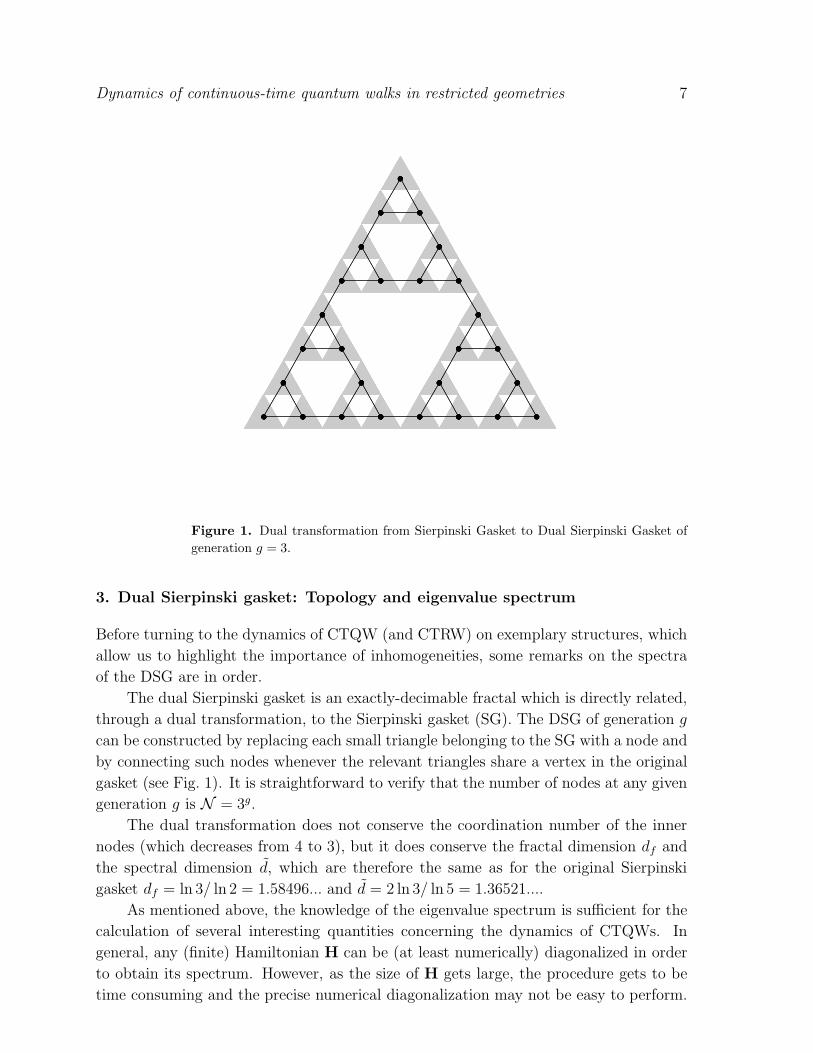
Figure 1. Dual transformation from Sierpinski Gasket to Dual Sierpinski Gasket of

generation g = 3.

3. Dual Sierpinski gasket: Topology and eigenvalue spectrum

Before turning to the dynamics of CTQW (and CTRW) on exemplary structures, which

allow us to highlight the importance of inhomogeneities, some remarks on the spectra

of the DSG are in order.

The dual Sierpinski gasket is an exactly-decimable fractal which is directly related,

through a dual transformation, to the Sierpinski gasket (SG). The DSG of generation g

can be constructed by replacing each small triangle belonging to the SG with a node and

by connecting such nodes whenever the relevant triangles share a vertex in the original

gasket (see Fig. 1). It is straightforward to verify that the number of nodes at any given

generation g is N = 3g.

The dual transformation does not conserve the coordination number of the inner

nodes (which decreases from 4 to 3), but it does conserve the fractal dimension df and

the spectral dimension d, which are therefore the same as for the original Sierpinski

gasket df = ln 3/ ln 2 = 1.58496... and d = 2 ln 3/ ln 5 = 1.36521....

As mentioned above, the knowledge of the eigenvalue spectrum is sufficient for the

calculation of several interesting quantities concerning the dynamics of CTQWs. In

general, any (finite) Hamiltonian H can be (at least numerically) diagonalized in order

to obtain its spectrum. However, as the size of H gets large, the procedure gets to be

time consuming and the precise numerical diagonalization may not be easy to perform.


Remarkably, the eigenvalue spectrum of the DSG Laplacian matrix can be determined

at any generation through the following iterative procedure; for more details we refer to

[34, 35]: At any given generation g the spectrum includes the non-degenerate eigenvalue

λN = 0, the eigenvalue 3 with degeneracy (3g−1 + 3)/2 and the eigenvalue 5 with

degeneracy (3g−1 − 1)/2. Moreover, given the eigenvalue spectrum at generation g − 1,

each non-vanishing eigenvalue λg−1 corresponds to two new eigenvalues λ±g according to

λ±g =5 ±

√

25 − 4λg−1

2; (14)

both λ+g and λ−g inherit the degeneracy of λg−1. The eigenvalue spectra is therefore

bounded in [0, 5]. As explained in [34], at any generation g, we can calculate the

degeneracy of each distinct eigenvalue: apart from λN whose degeneracy is 1, there are

2r distinct eigenvalues, each with degeneracy (3g−r−1+3)/2, being r = 0, 1, ..., g−1, and

2r distinct eigenvalues, each with degeneracy (3g−r−1 − 1)/2, being r = 0, 1, ..., g − 2.

As can be easily verified, the degeneracies sum up to N = 3g. Finally, notice that the

distribution of eigenvalues and their degeneracies are non-uniform and that the spectrum

is multifractal [34].

4. CTQWs on restricted geometries

4.1. Transfer probability

Results for the exact transition probability distribution πk,j(t) for STs and CTs have

already been given in Refs. [13, 31, 32], where it was shown that πk,j(t) depends

significantly on the starting node. Results for ultrametric structures are given in [33].

It is worth recalling here that the Cayley tree (CT) can be built by starting from

one node (root) connected to z nodes, which constitute the first shell. Each node of the

first shell is then connected to z − 1 new nodes, which constitute the second shell and

so forth, iteratively. Therefore, the M-th shell contains z(z − 1)M−1 nodes which are

at a chemical distance M from the root. Thus, the CT is a z-regular loop-free graph.

The numbers of sites in a CT of M shells is NM = [z(z − 1)M − 2]/(z − 2), hence the

correlated fractal dimension log(NM)/ log(M) goes to infinity for M → ∞, precluding

the possibility of embedding very large CT in any previously specified Euclidean lattice.

In the following we focus on finite 3-Cayley trees, which means that z is fixed and equal

to three for any internal site of the graph; furthermore, the number of shells (also called

generation) is finite (and therefore also the number of nodes is itself finite).

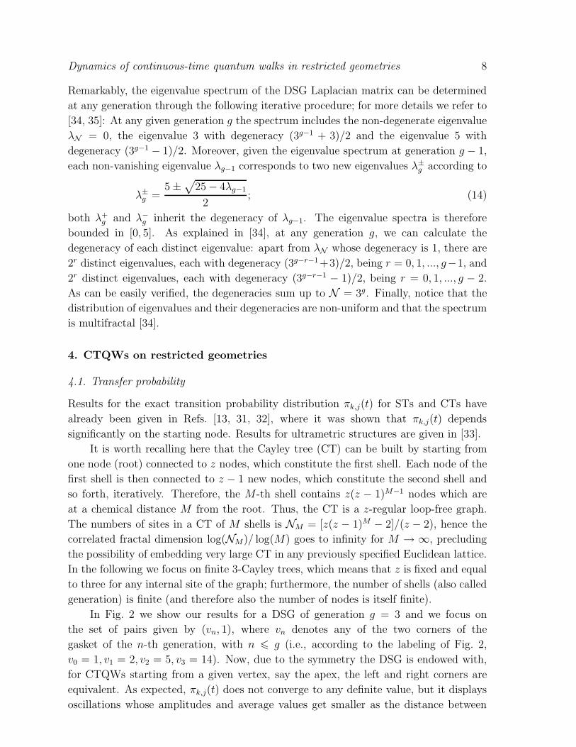
In Fig. 2 we show our results for a DSG of generation g = 3 and we focus on

the set of pairs given by (vn, 1), where vn denotes any of the two corners of the

gasket of the n-th generation, with n 6 g (i.e., according to the labeling of Fig. 2,

v0 = 1, v1 = 2, v2 = 5, v3 = 14). Now, due to the symmetry the DSG is endowed with,

for CTQWs starting from a given vertex, say the apex, the left and right corners are

equivalent. As expected, πk,j(t) does not converge to any definite value, but it displays

oscillations whose amplitudes and average values get smaller as the distance between


0 5 10 15 200

0.2

0.4

0.6

0.8

1

t(γ−1)

πk

,1(t

)

k = 1k = 2k = 5k = 14

1

2

5

14 18

10

43

79

Figure 2. Exact probability πk,1(t) for the CTQW starting from the apex (site j = 1)

to reach sites k = 1, 2, 5 and 14. The k-sites are the left corners at generations g = 0, 1, 2

and 3, respectively.

the sites 1 and vn increases. This suggests, at least when starting from a main vertex,

that the CTQW stays mainly localized at the origin and its neighbourhood.

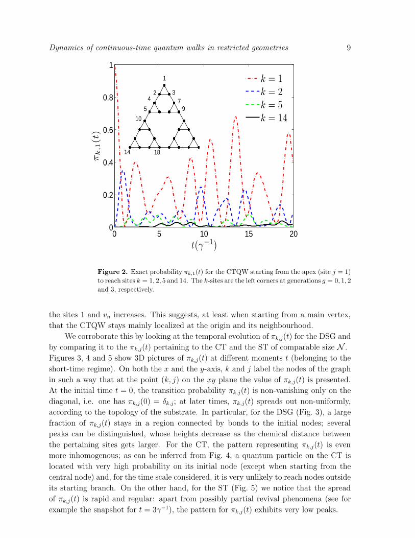
We corroborate this by looking at the temporal evolution of πk,j(t) for the DSG and

by comparing it to the πk,j(t) pertaining to the CT and the ST of comparable size N .

Figures 3, 4 and 5 show 3D pictures of πk,j(t) at different moments t (belonging to the

short-time regime). On both the x and the y-axis, k and j label the nodes of the graph

in such a way that at the point (k, j) on the xy plane the value of πk,j(t) is presented.

At the initial time t = 0, the transition probability πk,j(t) is non-vanishing only on the

diagonal, i.e. one has πk,j(0) = δk,j; at later times, πk,j(t) spreads out non-uniformly,

according to the topology of the substrate. In particular, for the DSG (Fig. 3), a large

fraction of πk,j(t) stays in a region connected by bonds to the initial nodes; several

peaks can be distinguished, whose heights decrease as the chemical distance between

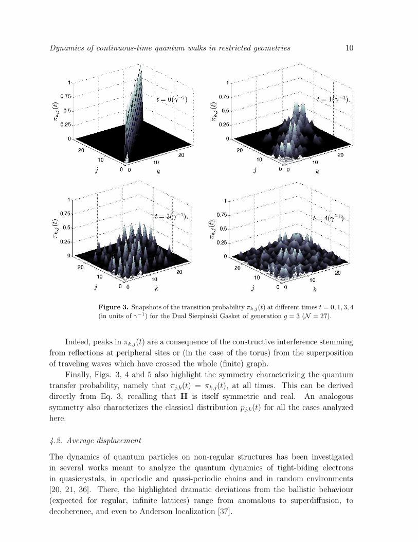
the pertaining sites gets larger. For the CT, the pattern representing πk,j(t) is even

more inhomogenous; as can be inferred from Fig. 4, a quantum particle on the CT is

located with very high probability on its initial node (except when starting from the

central node) and, for the time scale considered, it is very unlikely to reach nodes outside

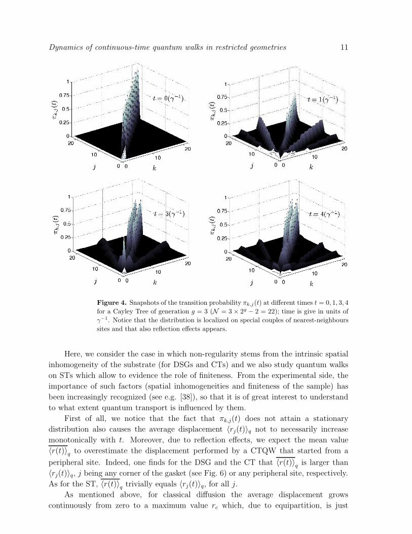
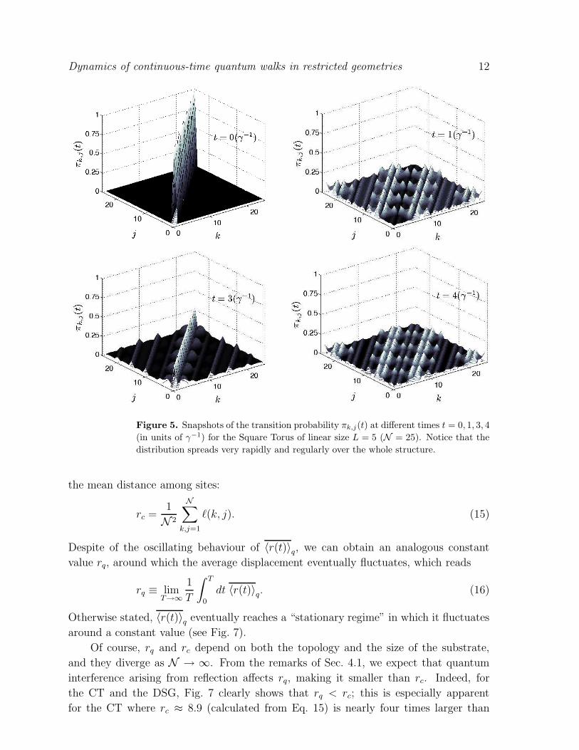
its starting branch. On the other hand, for the ST (Fig. 5) we notice that the spread

of πk,j(t) is rapid and regular: apart from possibly partial revival phenomena (see for

example the snapshot for t = 3γ−1), the pattern for πk,j(t) exhibits very low peaks.


Figure 3. Snapshots of the transition probability πk,j(t) at different times t = 0, 1, 3, 4

(in units of γ−1) for the Dual Sierpinski Gasket of generation g = 3 (N = 27).

Indeed, peaks in πk,j(t) are a consequence of the constructive interference stemming

from reflections at peripheral sites or (in the case of the torus) from the superposition

of traveling waves which have crossed the whole (finite) graph.

Finally, Figs. 3, 4 and 5 also highlight the symmetry characterizing the quantum

transfer probability, namely that πj,k(t) = πk,j(t), at all times. This can be derived

directly from Eq. 3, recalling that H is itself symmetric and real. An analogous

symmetry also characterizes the classical distribution pj,k(t) for all the cases analyzed

here.

4.2. Average displacement

The dynamics of quantum particles on non-regular structures has been investigated

in several works meant to analyze the quantum dynamics of tight-biding electrons

in quasicrystals, in aperiodic and quasi-periodic chains and in random environments

[20, 21, 36]. There, the highlighted dramatic deviations from the ballistic behaviour

(expected for regular, infinite lattices) range from anomalous to superdiffusion, to

decoherence, and even to Anderson localization [37].



for a Cayley Tree of generation g = 3 (N = 3 × 2g − 2 = 22); time is give in units of

γ−1. Notice that the distribution is localized on special couples of nearest-neighbours

sites and that also reflection effects appears.

Here, we consider the case in which non-regularity stems from the intrinsic spatial

inhomogeneity of the substrate (for DSGs and CTs) and we also study quantum walks

on STs which allow to evidence the role of finiteness. From the experimental side, the

importance of such factors (spatial inhomogeneities and finiteness of the sample) has

been increasingly recognized (see e.g. [38]), so that it is of great interest to understand

to what extent quantum transport is influenced by them.

First of all, we notice that the fact that πk,j(t) does not attain a stationary

distribution also causes the average displacement 〈rj(t)〉q not to necessarily increase

monotonically with t. Moreover, due to reflection effects, we expect the mean value

〈r(t)〉q to overestimate the displacement performed by a CTQW that started from a

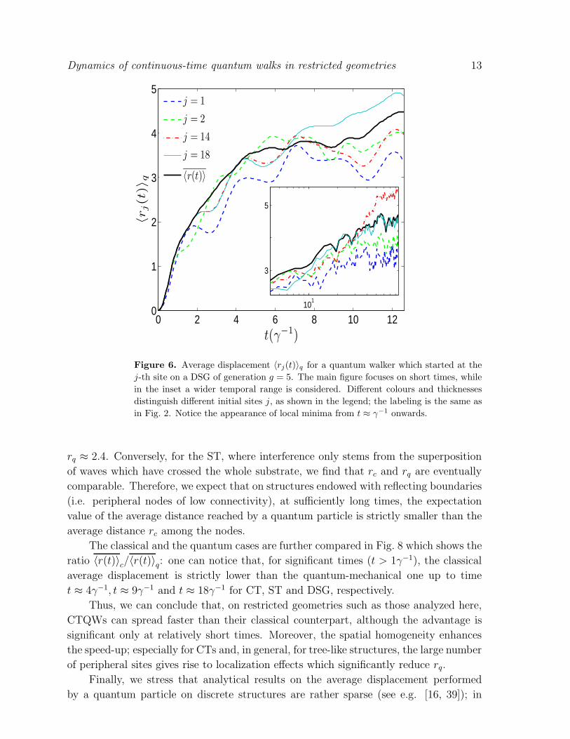
peripheral site. Indeed, one finds for the DSG and the CT that 〈r(t)〉q is larger than

〈rj(t)〉q, j being any corner of the gasket (see Fig. 6) or any peripheral site, respectively.

As for the ST, 〈r(t)〉q trivially equals 〈rj(t)〉q, for all j.

As mentioned above, for classical diffusion the average displacement grows

continuously from zero to a maximum value rc which, due to equipartition, is just



(in units of γ−1) for the Square Torus of linear size L = 5 (N = 25). Notice that the

distribution spreads very rapidly and regularly over the whole structure.

the mean distance among sites:

rc =1

N 2

N∑

k,j=1

ℓ(k, j). (15)

Despite of the oscillating behaviour of 〈r(t)〉q, we can obtain an analogous constant

value rq, around which the average displacement eventually fluctuates, which reads

rq ≡ limT→∞

1

T

∫ T

0

dt 〈r(t)〉q. (16)

Otherwise stated, 〈r(t)〉q eventually reaches a “stationary regime” in which it fluctuates

around a constant value (see Fig. 7).

Of course, rq and rc depend on both the topology and the size of the substrate,

and they diverge as N → ∞. From the remarks of Sec. 4.1, we expect that quantum

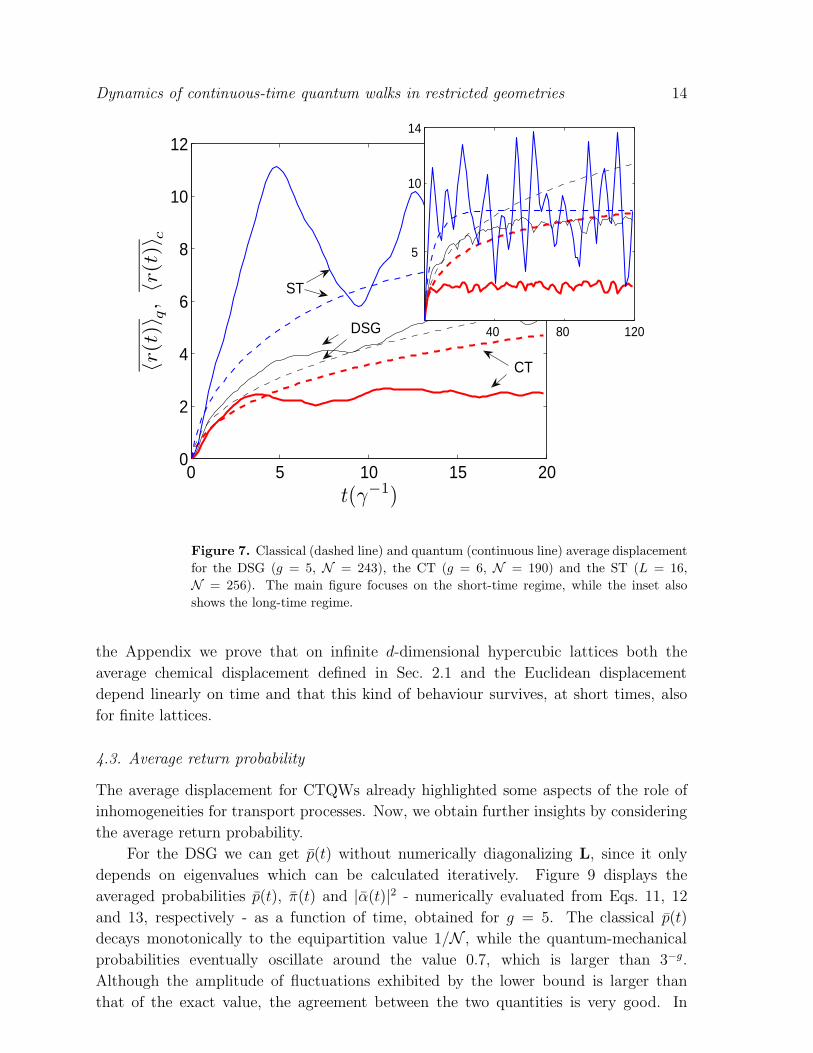
interference arising from reflection affects rq, making it smaller than rc. Indeed, for

the CT and the DSG, Fig. 7 clearly shows that rq < rc; this is especially apparent

for the CT where rc ≈ 8.9 (calculated from Eq. 15) is nearly four times larger than


0 2 4 6 8 10 120

1

2

3

4

5

t(γ−1)

〈rj(t)〉 q

j = 1

j = 2

j = 14

j = 18

〈r(t)〉

101

3

5

Figure 6. Average displacement 〈rj(t)〉q for a quantum walker which started at the

j-th site on a DSG of generation g = 5. The main figure focuses on short times, while

in the inset a wider temporal range is considered. Different colours and thicknesses

distinguish different initial sites j, as shown in the legend; the labeling is the same as

in Fig. 2. Notice the appearance of local minima from t ≈ γ−1 onwards.

rq ≈ 2.4. Conversely, for the ST, where interference only stems from the superposition

of waves which have crossed the whole substrate, we find that rc and rq are eventually

comparable. Therefore, we expect that on structures endowed with reflecting boundaries

(i.e. peripheral nodes of low connectivity), at sufficiently long times, the expectation

value of the average distance reached by a quantum particle is strictly smaller than the

average distance rc among the nodes.

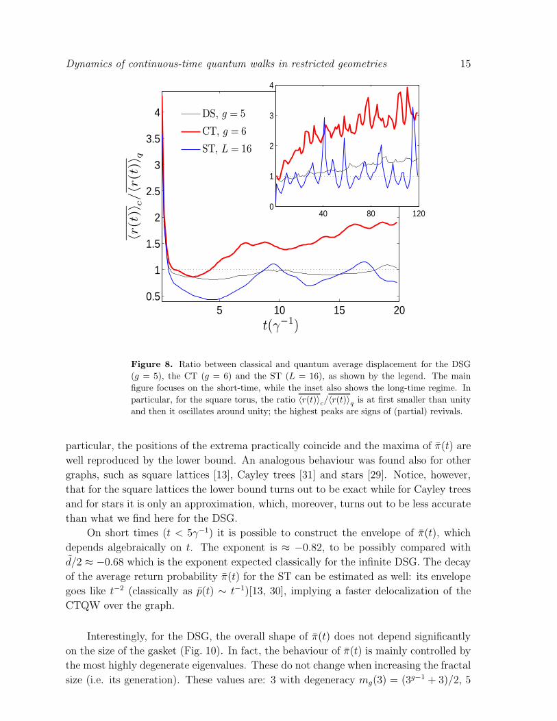
The classical and the quantum cases are further compared in Fig. 8 which shows the

ratio 〈r(t)〉c/〈r(t)〉q: one can notice that, for significant times (t > 1γ−1), the classical

average displacement is strictly lower than the quantum-mechanical one up to time

t ≈ 4γ−1, t ≈ 9γ−1 and t ≈ 18γ−1 for CT, ST and DSG, respectively.

Thus, we can conclude that, on restricted geometries such as those analyzed here,

CTQWs can spread faster than their classical counterpart, although the advantage is

significant only at relatively short times. Moreover, the spatial homogeneity enhances

the speed-up; especially for CTs and, in general, for tree-like structures, the large number

of peripheral sites gives rise to localization effects which significantly reduce rq.

Finally, we stress that analytical results on the average displacement performed

by a quantum particle on discrete structures are rather sparse (see e.g. [16, 39]); in


0 5 10 15 200

2

4

6

8

10

12

t(γ−1)

〈r(t

)〉q,〈r

(t)〉

c

40 80 120

5

10

14

DSG

ST

CT

Figure 7. Classical (dashed line) and quantum (continuous line) average displacement

for the DSG (g = 5, N = 243), the CT (g = 6, N = 190) and the ST (L = 16,

N = 256). The main figure focuses on the short-time regime, while the inset also

shows the long-time regime.

the Appendix we prove that on infinite d-dimensional hypercubic lattices both the

average chemical displacement defined in Sec. 2.1 and the Euclidean displacement

depend linearly on time and that this kind of behaviour survives, at short times, also

for finite lattices.

4.3. Average return probability

The average displacement for CTQWs already highlighted some aspects of the role of

inhomogeneities for transport processes. Now, we obtain further insights by considering

the average return probability.

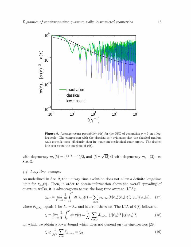
For the DSG we can get p(t) without numerically diagonalizing L, since it only

depends on eigenvalues which can be calculated iteratively. Figure 9 displays the

averaged probabilities p(t), π(t) and |α(t)|2 - numerically evaluated from Eqs. 11, 12

and 13, respectively - as a function of time, obtained for g = 5. The classical p(t)

decays monotonically to the equipartition value 1/N , while the quantum-mechanical

probabilities eventually oscillate around the value 0.7, which is larger than 3−g.

Although the amplitude of fluctuations exhibited by the lower bound is larger than

that of the exact value, the agreement between the two quantities is very good. In


5 10 15 200.5

1

1.5

2

2.5

3

3.5

4

t(γ−1)

〈r(t

)〉c/〈r

(t)〉

q

40 80 1200

1

2

3

4

DS, g = 5

CT, g = 6

ST, L = 16

Figure 8. Ratio between classical and quantum average displacement for the DSG

(g = 5), the CT (g = 6) and the ST (L = 16), as shown by the legend. The main

figure focuses on the short-time, while the inset also shows the long-time regime. In

particular, for the square torus, the ratio 〈r(t)〉c/〈r(t)〉q is at first smaller than unity

and then it oscillates around unity; the highest peaks are signs of (partial) revivals.

particular, the positions of the extrema practically coincide and the maxima of π(t) are

well reproduced by the lower bound. An analogous behaviour was found also for other

graphs, such as square lattices [13], Cayley trees [31] and stars [29]. Notice, however,

that for the square lattices the lower bound turns out to be exact while for Cayley trees

and for stars it is only an approximation, which, moreover, turns out to be less accurate

than what we find here for the DSG.

On short times (t < 5γ−1) it is possible to construct the envelope of π(t), which

depends algebraically on t. The exponent is ≈ −0.82, to be possibly compared with

d/2 ≈ −0.68 which is the exponent expected classically for the infinite DSG. The decay

of the average return probability π(t) for the ST can be estimated as well: its envelope

goes like t−2 (classically as p(t) ∼ t−1)[13, 30], implying a faster delocalization of the

CTQW over the graph.

Interestingly, for the DSG, the overall shape of π(t) does not depend significantly

on the size of the gasket (Fig. 10). In fact, the behaviour of π(t) is mainly controlled by

the most highly degenerate eigenvalues. These do not change when increasing the fractal

size (i.e. its generation). These values are: 3 with degeneracy mg(3) = (3g−1 + 3)/2, 5


10−1

100

101

102

103

10−6

10−4

10−2

100

t(γ−1)

π(t)

,|α

(t)|2

,p(t)

exact valueclassicallower bound

Figure 9. Average return probability π(t) for the DSG of generation g = 5 on a log-

log scale. The comparison with the classical p(t) evidences that the classical random

walk spreads more efficiently than its quantum-mechanical counterpart. The dashed

line represents the envelope of π(t).

with degeneracy mg(5) = (3g−1 − 1)/2, and (5 ±√

13)/2 with degeneracy mg−1(3), see

Sec. 3.

4.4. Long time averages

As underlined in Sec. 2, the unitary time evolution does not allow a definite long-time

limit for πk,j(t). Then, in order to obtain information about the overall spreading of

quantum walks, it is advantageous to use the long time average (LTA):

χk,j ≡ limT→∞

1

T

∫ T

0

dt πk,j(t) =∑

n,m

δλn,λm〈k|ψn〉〈ψn|j〉〈j|ψm〉〈ψm|k〉, (17)

where δλn,λmequals 1 for λn = λm and is zero otherwise. The LTA of π(t) follows as

χ ≡ limT→∞

1

T

∫ T

0

dt π(t) =1

N∑

n,m,j

δλn,λm|〈j|ψn〉|2 |〈j|ψm〉|2, (18)

for which we obtain a lower bound which does not depend on the eigenvectors [29]:

χ ≥ 1

N 2

∑

n,m

δλn,λm≡ χlb. (19)


0 10 20 30 40

10−4

10−3

10−2

10−1

100

t(γ−1)

π(t

),|α

(t)|2

,p(t

)

π(t), g = 4

|α(t)|2, g = 4

p(t), g = 4

π(t), g = 5

|α(t)|2, g = 5

p(t), g = 5

Figure 10. Average return probability π(t) for the DSG of generation g = 4 (bright

colour) and g = 5 (dark colour). Its lower bound |α(t)|2 (dashed line) and the classical

p(t) (dotted line) are also depicted, as shown by the legend.

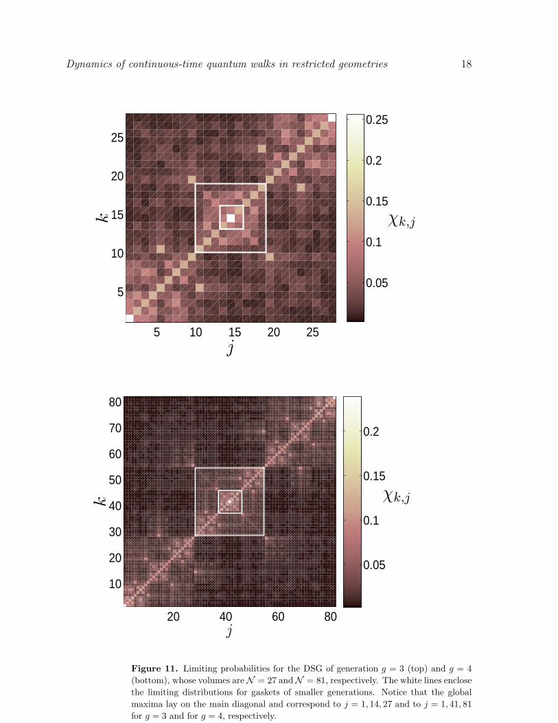
We first consider the DSG for which Fig. 11 shows χk,j as a contour plot, whose

axes are labeled by the nodes k = 1, ...,N and j = 1, ...,N . Bright colours correspond

to large, dark ones to small LTAs. First of all, we notice that the LTAs are far from

being homogeneous and, hence, are not equipartioned. In particular, the values on the

main diagonal are high, meaning that CTQWs have a high LTA probability to be at

the starting node.

The inhomogeneity of the pattern mirrors the lack of translation invariance of the

DSG itself. For instance, v being the label assigned to any vertex of the main triangle,

χv,v is a global maximum; off-diagonal local maxima correspond to couples of connected

nodes belonging to different minor triangles of generation g−1. This allows to establish

a mapping between the pattern of χk,j and the structure of the relevant DSG. Indeed, as

suggested by the white delimiting lines in Fig. 11, the patterns of the LTA distributions

exhibit self-similarity.

As for χ and its lower bound χlb, we recall that the former can be calculated

numerically, once all eigenvalues and eigenvectors of the Laplacian operator are known

(Eq. 18), while for the latter the knowledge of the eigenvalue spectrum is sufficient

(Eq. 19). Since the spectrum of the DSG is known, we can calculate χlb analytically.

Recalling the results of Sec. 3, at generation g the spectrum of L displays N distinct


5 10 15 20 25

5

10

15

20

25

j

k

0.05

0.1

0.15

0.2

0.25

χk,j

20 40 60 80

10

20

30

40

50

60

70

80

j

k

0.05

0.1

0.15

0.2

χk,j

Figure 11. Limiting probabilities for the DSG of generation g = 3 (top) and g = 4

(bottom), whose volumes are N = 27 and N = 81, respectively. The white lines enclose

the limiting distributions for gaskets of smaller generations. Notice that the global

maxima lay on the main diagonal and correspond to j = 1, 14, 27 and to j = 1, 41, 81

for g = 3 and for g = 4, respectively.


eigenvalues, where

N =

g−1∑

r=0

2r +

g−2∑

r=0

2r + 1 = 3 × 2g−1 − 1.

We call the set of distinct eigenvalues {λi}i=1,...,N . Being m(λi) the degeneracy of the

eigenvalue λi, we can write

N 2χlb =

N∑

n,m=1

δλn,λm=

N∑

n=1

m(λn) =

N∑

i=1

[

m(λi)]2

.

Now, we go over to the space of distinct degeneracies, each corresponding to a number

ρ of distinct eigenvalues and we get the final, explicit formula

χ ≥ χlb =1

N 2

2g∑

r=0

[m(r)]2ρ(m(r))

=1

N 2

{

g−1∑

r=0

[

3g−r−1 + 3

2

]2

× 2r +

g−2∑

r=0

[

3g−r−1 − 1

2

]2

× 2r + 1

}

=1

32g

[

3g

(

1 +3g

14

)

+10

72g − 3

2

]

>1

3g. (20)

Interestingly, in the limit g → ∞, the LTA χ is finite:

χ ≥ limg→∞

χlb =1

14,

and χlb reaches this asymptotic value from above.

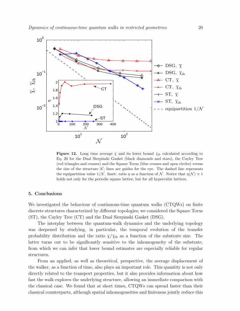
In Fig. 12 we show, as functions of N , χ and its lower bound, calculated from

Eq. 18 and from Eq. 20. For comparison, the same quantities obtained for CTs and STs

are also depicted. In the latter case, due to the regularity and periodicity of the lattice

[40], the lower bound actually coincides with the exact value. For all cases considered,

χ is larger than the equipartion value (given by the dashed line).

The inset of Fig. 12 shows the ratio

η(N ) ≡ χ

χlb.

Obviously, the closer η is to 1, the better χlb approximates χ. In this sense, the lower

bound calculated for CTs is not as good an approximation to χ as it is for the DSG

and for the ST. For the CT, χlb definitely underestimates, being about half the exact

value of χ. The quantity η(N ) may act as a measure of the inhomogeneity of a given

substrate. Practically, when dealing with a large sized, sufficiently regular structure, we

can get information about the localization of a quantum particle moving on it simply

through χlb, thus avoiding the (lengthy) evaluation of the eigenvector set.


101

102

10−2

10−1

100

N

χ,

χlb

0 100 200 300 4001

1.2

1.4

1.6

1.8

2

N

η

DSG, χ

DSG, χlb

CT, χ

CT, χlb

ST, χ

ST, χlb

equipartition 1/N

CT

ST

DSG

Figure 12. Long time average χ and its lower bound χlb calculated according to

Eq. 20 for the Dual Sierpinski Gasket (black diamonds and stars), the Cayley Tree

(red triangles and crosses) and the Square Torus (blue crosses and open circles) versus

the size of the structure N ; lines are guides for the eye. The dashed line represents

the equipartition value 1/N . Inset: ratio η as a function of N . Notice that η(N ) ≡ 1

holds not only for the periodic square lattice, but for all hypercubic lattices.

5. Conclusions

We investigated the behaviour of continuous-time quantum walks (CTQWs) on finite

discrete structures characterized by different topologies; we considered the Square Torus

(ST), the Cayley Tree (CT) and the Dual Sierpinski Gasket (DSG).

The interplay between the quantum-walk dynamics and the underlying topology

was deepened by studying, in particular, the temporal evolution of the transfer

probability distribution and the ratio χ/χlb as a function of the substrate size. The

latter turns out to be significantly sensitive to the inhomogeneity of the substrate,

from which we can infer that lower bound estimates are especially reliable for regular

structures.

From an applied, as well as theoretical, perspective, the average displacement of

the walker, as a function of time, also plays an important role. This quantity is not only

directly related to the transport properties, but it also provides information about how

fast the walk explores the underlying structure, allowing an immediate comparison with

the classical case. We found that at short times, CTQWs can spread faster than their

classical counterparts, although spatial inhomogeneities and finiteness jointly reduce this


effect. In the Appendix we prove that for infinite d-dimensional hypercubic lattices, at

long times both the average chemical and the Euclidean displacements depend linearly

on time (i.e. the motion is ballistic); for finite lattices this kind of behaviour holds at

relatively short times only.

Acknowledgements

EA thanks the Italian Foundation “Angelo della Riccia” for financial support. Support

from the Deutsche Forschungsgemeinschaft (DFG), the Fonds der Chemischen Industrie

and the Ministry of Science, Research and the Arts of Baden-Wurttemberg (AZ: 24-

7532.23-11-11/1) is gratefully acknowledged.

Appendix A. Average chemical displacement on hypercubic lattices

Here we consider infinite d-dimensional hypercubic lattices and, by exploiting their

translational invariance, we prove that on them the average chemical displacements of

CTQWs, as defined in Sec. 2.1, depend linearly on time. We first focus on the infinite

discrete chain, then we consider the generic d-dimensional case and finally we analyze

the two-dimensional lattice.

For a ring of length N , by exploiting the Bloch states, we have [41]

αk,j(t) =1√N

∑

l

e−iλlte−il(k−j), (A.1)

where λl is the l-th eigenvalue of the Laplacian matrix L associated with the ring. In

the limit N → ∞ we are allowed to replace the sum over l by an integral, obtaining

limN→∞

αk,j(t) = ik−je−i2tJk−j(2t), (A.2)

where Jk(z) is the Bessel function of the first kind. In the calculation of the transfer

probability πk,j(t) the phase factor vanishes and we have πk,j(t) = J2k−j(2t), which can

be restated as

πk,0(t) = J2k (2t), (A.3)

due to the translational invariance of the structure. Clearly (in agreement with πk,0(t)

being a probability distribution), one has for all t+∞∑

k=−∞

πk,0(t) =

+∞∑

k=−∞

J2k (2t) = J2

0 (2t) + 2

∞∑

k=1

J2k(2t) = 1, (A.4)

the last equality being based on Jk(z) = (−1)kJ−k(z) and on Eq. 8.536.3 in [42].

Now, the average chemical displacement of a CTQW which starts from 0 and moves

on an infinite chain (subscript q, 1) follows from Eq. 5 as

〈r0(t)〉q,1 = 〈r(t)〉q,1 =∑

k∈V

ℓ(k, 0) J2k(2t) (A.5)

=∞

∑

k=−∞

|k| J2k(2t) = 2

∞∑

k=1

k J2k(2t).

https://www.researchgate.net/publication/225092415_In_Table_of_Integrals_Series_and_Products?el=1_x_8&enrichId=rgreq-552e4f8a72b37b054a4f86789d7d8930-XXX&enrichSource=Y292ZXJQYWdlOzIyMDk1MTk7QVM6MTAxMzQwODE4NzA2NDM1QDE0MDExNzI5NDMyMTQ=


Here, in the first equality we dropped the subscript 0 due to the equivalence between

the sites and in the last equality we exploited the symmetry of the Bessel functions,

J2−k(z) = J2

k (z). Now, recalling the recursion formula Eq. 8.471.1 in [42]

Jk−1(z) + Jk+1(z) =2k

zJk(z), (A.6)

we can write

2∞

∑

k=1

k J2k (z) = z

∞∑

k=1

[Jk−1(z) Jk(z) + Jk(z) Jk+1(z)] ≡ zJ (z), (A.7)

by defining the function J (z). Hence

〈rk

(z

2

)

〉q,1 = zJ (z), (A.8)

where we put 2t = z. The squared Bessel function J2k (z) is almost everywhere positive

and the analysis of its zeros allows to state that, for t > 0, the sum appearing in the

left-hand-side of Eq. A.8 is strictly positive; the same holds therefore for J (z), for which

we also notice from Eq. A.7 that J (0) = 0. Moreover, through the following recursion

formula, Eq. 8.471.2 in [42]

2∂

∂zJk(z) = Jk−1(z) − Jk+1(z), (A.9)

it follows by directly differentiating J (z) and rearranging the terms

d

dzJ (z) =

J0(z)[J0(z) + J2(z)]

2=J0(z)J1(z)

z, (A.10)

where in the last expression we again used Eq. A.6 for k = 1. The indefinite integral of

Eq. A.10 is (see Eq. 5.53 in [42])

J (z) = z J20 (z) + z J2

1 (z) − J0(z)J1(z) + C, (A.11)

as can be simply verified by differentiating Eq. A.11 and using Eqs. A.6 and A.9.

Furthermore, since J (0) = 0, we have C = 0.

Therefore, the following, for us fundamental, relation holds:∞

∑

k=1

k J2k(z) =

z

2[z J2

0 (z) + z J21 (z) − J0(z)J1(z)]. (A.12)

Now, from Eqs. A.5 and A.12 we get the exact expression for the average chemical

displacement

〈r(z

2

)

〉q,1 = z[

z J0(z)2 + z J1(z)

2 − J0(z)J1(z)]

. (A.13)

For large z = 2t (i.e. long times) we can use the expansion (see Eq. 8.451.1 in [42])

Jk(z) =

√

2

πz

[

cos

(

z − kπ

2− π

4

)

+O

(

1

z

)]

. (A.14)

Consequently, inserting Eq. A.14 for J0(z) and J1(z) into A.13, we infer that the long

time behaviour of the average chemical CTQW displacement on an infinite chain obeys

〈r(t)〉q,1 ∼4t

π. (A.15)



0 5 10 150

2

4

6

8

10

12

t(γ−1)

〈r(t

)〉q,2

L = 7

L = 9

L = 15

L = 19

L = 19 Euclidean

8t/π

6t/π

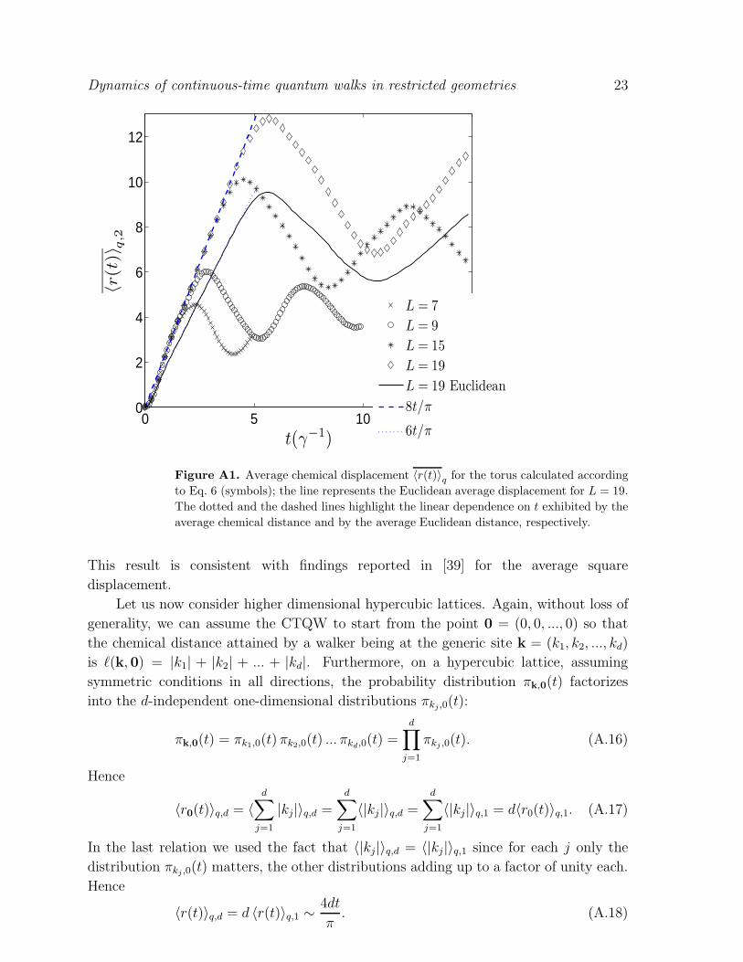
Figure A1. Average chemical displacement 〈r(t)〉q for the torus calculated according

to Eq. 6 (symbols); the line represents the Euclidean average displacement for L = 19.

The dotted and the dashed lines highlight the linear dependence on t exhibited by the

average chemical distance and by the average Euclidean distance, respectively.

This result is consistent with findings reported in [39] for the average square

displacement.

Let us now consider higher dimensional hypercubic lattices. Again, without loss of

generality, we can assume the CTQW to start from the point 0 = (0, 0, ..., 0) so that

the chemical distance attained by a walker being at the generic site k = (k1, k2, ..., kd)

is ℓ(k, 0) = |k1| + |k2| + ... + |kd|. Furthermore, on a hypercubic lattice, assuming

symmetric conditions in all directions, the probability distribution πk,0(t) factorizes

into the d-independent one-dimensional distributions πkj ,0(t):

πk,0(t) = πk1,0(t) πk2,0(t) ... πkd,0(t) =

d∏

j=1

πkj ,0(t). (A.16)

Hence

〈r0(t)〉q,d = 〈d

∑

j=1

|kj|〉q,d =

d∑

j=1

〈|kj|〉q,d =

d∑

j=1

〈|kj|〉q,1 = d〈r0(t)〉q,1. (A.17)

In the last relation we used the fact that 〈|kj|〉q,d = 〈|kj|〉q,1 since for each j only the

distribution πkj ,0(t) matters, the other distributions adding up to a factor of unity each.

Hence

〈r(t)〉q,d = d 〈r(t)〉q,1 ∼4dt

π. (A.18)


In particular, for the square lattice we have

〈r(t)〉q,2 ∼8t

π, (A.19)

which was used in Fig. A1 (dashed line) to fit data relevant to the average chemical

displacement performed by a CTQW on square tori of different (finite) sizes. As can

be seen from the figure, the ballistic behaviour also holds for finite lattices, but for

relatively short times only: at longer times the finiteness of the lattice starts to matter

and the product of Bessel functions in Eq. A.16 ceases to be a good approximation of

the transfer probability. When the waves associated with CTQWs have crossed the

whole lattice, interference effects start to occur and 〈r(t)〉q,2 exhibits a non-monotonic

behaviour. From the same figure we also notice that theO(1/t) contributions of Eq. A.14

get to be negligible for t > 1 γ−1.

In Fig. A1 we also show data for the average Euclidean displacement which displays

a ballistic behaviour at short times as well. Indeed, for a hypercubic lattice of arbitrary

dimension d, the following relation holds (see e.g. [43])

1√3ℓ(k, j) ≤ ||k − j|| ≤ ℓ(k, j) (A.20)

where ||k− j|| denotes the Euclidean distance between the lattice points k and j chosen

arbitrarily. By averaging each term of the previous equation with respect to the transfer

probability πk,j(t) (we can again exploit the translational invariance of the substrate and

fix j = 0), we find that the average Euclidean distance also scales linearly with time with

a multiplicative factor bounded between 4d/(√

3π) ≈ 2.31d/π and 4d/π. In particular,

for the square torus of size L = 19 considered in Fig. A1, we find that at relatively short

times the average Euclidean distance scales as 6t/π.

References

[1] Kempe J 2003 Contemp. Physics 44 307

[2] Sanders BC, Bartlett SD, Tregenna B and Knight PL 2003 Phys. Rev. A 67 042305

[3] Lahini Y, Avidan A, Pozzi F, Sorel M, Morandotti R, Christodoulides DN, and Silberberg Y 2008

Phys. Rev. Lett. 100 013906

[4] Dur W, Raussendorf R, Kendon VM and Briegel H-J 2002 Phys. Rev. A 66 052319

[5] Cote R, Russell A, Eyler EE and Gould PL 2006 New J. Phys. 8 156

[6] Zou X, Dong Y and Guo G 2006 New J. Phys. 8 81

[7] Ryan CA, Laforest M, Boileau JC and Laflamme R 2005 Phys. Rev. A 72 062317

[8] Mulken O, Blumen A, Amthor T, Giese C, Reetz-Lamour M and Weidemuller M 2007 Phys. Rev.

Lett. 99 090601

[9] Aharonov Y, Davidovich L and Zagury N 1993 Phys. Rev. A 48 1687

[10] Farhi E and Gutmann S 1998 Phys. Rev. A 58 915

[11] Strauch FW 2006 Phys. Rev. A 74 030301(R)

[12] Stefanak M, Jex I and Kiss T 2008 Phys. Rev. Lett. 100 020501

[13] Volta A, Mulken O and Blumen A 2006 J. Phys. A 39 14997

[14] Mulken O, Pernice V and Blumen A 2007 Phys. Rev. E 76 051125

[15] ben-Avraham D and Havlin S, Diffusion and Reactions in Fractals and Disordered Systems,

(Cambridge University Press, 2001).


[16] J. Vidal, R. Mosseri and J. Bellissard 1999 J. Phys. A 32 2361

[17] Williams CP 2001 Computing in Science and Engineering 3, 2 44

[18] Ambainis A 2004 SIGACT News 35 22

[19] Magniez F, Nayak A, Roland J and Santha M, in Proceedings of ACM Symposium on Theory of

Computation (STOC’07) (ACM Press, New York, 2007), p.575

[20] Yin Y, Katsanos DE and Evangelou SN 2008 Phys. Rev. A 77 022302

[21] Yuan HQ, Grimm U, Repetowicz P and Schreiber M 2000 Phys. Rev. B 62 15569

[22] Graph Theory, Combinatorics, and Applications, Vol. 2, Ed. Y. Alavi, G. Chartrand, O.R.

Oellermann, A.J. Schwenk, Wiley, 1991.

[23] Di Vincenzo DP 1995 Science 270 255

[24] Childs AM and Goldstone J 2004 Phys. Rev. A 70 022314

[25] Mulken O, Volta A and Blumen A 2005 Phys. Rev. A 72 042334

[26] Weiss GH, Aspects and Applications of the Random Walk, (North-Holland Press, 1994)

[27] Aharonov D, Ambainis A, Kempe J and Vazirani U, in Proceedings of ACM Symposium on Theory

of Computation (STOC’01) (ACM Press, New York, 2001), p.50.

[28] Aarao Reis FDA 1995 J. Phys. A 28 6277

[29] Mulken O 2007 arXiv:0710.3453

[30] Mulken O and Blumen A 2006 Phys. Rev. E 73 066117

[31] Mulken O, Bierbaum V and Blumen A 2006 J. Chem. Phys. 124 124905

[32] Konno N 2006 Quantum Probability and Related Topics 9, 2 287

[33] Konno N 2006 Int. J. Quant. Inf. 4, 6 1023

[34] Cosenza MG and Kapral R 1992 Phys. Rev. A 46 1850

[35] Blumen A and Jurjiu A 2002 J. Chem. Phys. 116 2636

[36] Cerovski VZ, Schreiber M and Grimm U 2005 Phys. Rev. B 72 054203

[37] Anderson PW 1958 Phys. Rev. 109 1492

[38] Monastyrsky MI, Topology in Condensed Matter, Springer Series In Solid-State Sciences, Springer-

Verlag Berlin Heidelberg 2006

[39] Katsanos DE, Evangelou SN and Xiong SJ 1995 Phys. Rev. B 51 895

[40] Blumen A, Bierbaum V and Mulken O 2006 Physica A 371 10

[41] Mulken O and Blumen A 2005 Phys. Rev. E 71 036128

[42] Gradshteyn IS and Ryzhik IM, Table of Integrals, Series and Products, Academic Press, Inc. 1965.

[43] Searcoid MO, Metric Spaces, Springer-Verlag, London 2007.

http://arXiv.org/abs/0710.3453



Dynamics of continuous-time quantum walks in restricted geometries

Documents

Transcript of Dynamics of continuous-time quantum walks in restricted geometries