Geometries et Dynamiques
364
TRAVAUX EN COURS Edit´ e par Khaled Sadallah & Abdelghani Zeghib G´ eom´ etries et Dynamiques LES COURS DU CIMPA CENTRE I NTERNATIONAL DE MATH ´ EMATIQUES PURES ET APPLIQU ´ EES HERMANN – ´ EDITEURS DES SCIENCES ET DES ARTS, PARIS
-
Upload
univ-paris5 -
Category
Documents
-
view
0 -
download
0
Transcript of Geometries et Dynamiques

TRAVAUX EN COURS
Edite par
Khaled Sadallah & Abdelghani Zeghib
Geometries et Dynamiques
LES COURS DU CIMPACENTRE INTERNATIONAL DE MATHEMATIQUES PURES ET APPLIQUEES
HERMANN – EDITEURS DES SCIENCES ET DES ARTS, PARIS


Ecole CIMPA–UNESCO–El-OUED ALGERIEGeometries et Dynamiques riemanniennes et
pseudo-riemanniennes, et Applications
Geometries et Dynamiques
edite par
Khaled Sadallah & Abdelghani Zeghib
avec une preface de
Gerard Besson
COLLECTION TRAVAUX EN COURS
HERMANN – EDITEURS DES SCIENCES ET DES ARTS

Classification AMS : 53-06, 53A35, 53A30, 30F99, 30F30, 53A05, 53A10, 53C20, 22F30,37C10, 37C85, 57M25, 57S30, 83C05, 83C57
Mots-cles : geometrie differentielle, geometrie pseudo-riemannienne, surfaces de Riemann,surfaces minimales, espaces homogenes, Relativite generale, equation d’Einstein, trous noirs,systemes dynamiques, noeuds.
Key-words : differential geometry, pseudo-Riemannian geometry, Riemann surfaces, mini-mal surfaces, homogeneous spaces, general relativity, Einstein’s equation, black holes, dyna-mical systems, knots.
ISBN
2004, Hermann, editeurs des sciences et des arts, 293 rue Lecourbe, 75015 Paris
Tous droits de reproduction, meme fragmentaire, sous quelque forme que ce soit, y compris photographie, microfilm,bande magnetique, disque ou autre, reserves pour tous pays.

Preface
Reunir des mathematiciens dans un lieu isole et protege, loin du reste du monde, est unegrande tradition dans notre discipline. C’est une toute autre reunion qui fut organisee auxportes du Sahara en fevrier-mars 2005, sous l’egide du CIMPA (le bien nomme). Meme sile desert me fait penser aux ermites des temps anciens, nul sentiment de s’etre retire loindes hommes. C’est bien au contraire a une explosion de sensations, d’odeurs, de saveurs etdisons-le de vie a laquelle nous avons pu assister et participer, au milieu des coupoles d’ElOued Souf. Dans une Algerie en pleine guerison, il n’etait pas si aise pour les organisateurset pour nos hotes de mettre en place les conditions d’une rencontre reussie ; mais l’hospitaliteafricaine a fait son œuvre. En retrouvant nos collegues maghrebins que j’ai eu si peu l’oc-casion de rencontrer durant la derniere decennie j’ai compris ce qu’on entend par traditionmathematique ; malgre les difficultes de toutes sortes, on trouve toujours des gens assez fouspour s’enthousiasmer pour notre science. C’est une constatation rasserenante.
Le fascicule qui suit contient les textes des principaux cours ainsi que ceux de quelques-uns des exposes du GGTM (Groupement pour le developpement de la Geometrie et Topologieau Maghreb). Il s’agit de geometries et dynamiques ; on aura note le pluriel ! En parcourantcette monographie je suis epate par la qualite scientifique des documents presentes. Les courssont ce que devraient etre tout enseignement de base de geometrie. On y decouvre commentla cartographie et la mecanique des fluides conduisent a la belle theorie des surfaces de Rie-mann du point de vue complexe ou algebrique. On y retrouve les proprietes des courbes et dessurfaces ; il faut continuer a enseigner ces notions si riches dans nos universites. On y etudieaussi les structures geometriques, les espaces homogenes, la geometrie pseudo-riemannienneet l’emblematique geometrie lorentzienne qui conduit a la relativite. C’est la dynamique et sesapplications a la cosmologie qui closent ce panorama. A un moment ou l’analyse geometriquetient le haut du pave, grace a ses succes recents, il est important de ne pas negliger ces no-tions dont certaines sont malheureusement peu connues de beaucoup de geometres. Ce texterafraıchissant aux qualites pedagogiques exceptionnelles deviendra rapidement une referenceincontournable. Quant a la partie consacree au colloque GGTM, il suffit de la feuilleter pourconstater la solidite scientifique des articles presentes.
Au-dela des belles mathematiques je n’oublierai pas les vents de sable, le coucher de so-leil sur les dunes, le the a la menthe et ce collegue d’Alger qui part chaque annee marcherdans le grand sud desertique et qui m’a promis de m’emmener un jour. Une derniere anec-dote. Le jour de mon depart un ami algerien dont je tairais le nom mais qui se reconnaıtra m’aaccompagne a l’aeroport de Biskra, a trois heures de voiture d’El Oued. Il fallait de l’essenceet les pompes etaient fermees, alors, apres pas mal de tentatives infructueuses mon accompa-
v
gnateur decida de prendre un taxi que nous partageames avec d’autres. A l’arrivee a l’aeroporttous les passagers avaient deja embarque et il lui a fallu beaucoup de doigte et de diplomatiepour convaincre les autorites portuaires de me laisser monter dans l’avion. Cette capacite aimproviser des solutions sur le champ afin de resoudre des problemes a priori insurmontablesest typique d’un vrai mathematicien. Chapeau l’ami !
Gerard BessonGrenoble, mai 2008

Remerciements
Du 26 Fevrier au 10 Mars 2005, s’est tenue a El-Oued l’ecole :
CIMPA-UNESCO-ALGERIE« Geometries et Dynamiques Riemannienneset Pseudo-riemanniennes, et Applications ».
De l’avis de tous, cette ecole CIMPA d’El-Oued fut un evenement exceptionnel a tous lespoints de vue. Saluons tout d’abord la qualite des nombreux conferenciers et participants, quenous tenons a remercier... Il y a ensuite tous les autres acteurs, qui auront egalement contribuede maniere essentielle, tant par leur quantite et la qualite de leur travail. Nous remercions tousles organisateurs, y compris ceux qui ne sont pas cites dans le comite d’organisation. L’un desaspects le plus remarquable dans cet evenement fut la generosite singuliere de nos sponsorsqui nous ont recus avec chaleur, bonte et, disons-le, avec une certaine beaute. Leurs nomssont graves dans notre memoire et ceux de nos hotes. Nous avons fait le choix, difficile, dene pas citer leur nom, par egard pour ceux d’entre eux qui ont tenu a garder leur contributionanonyme. Toute la ville d’El-Oued, ses forces vives, ses industriels, ses intellectuels, sesadministratifs..., et une grande partie de la population ont resonne et vibre avec nous. Nousavons ete enchantes, combles et charmes par cette ambiance inoubliable.
K. Sadallah & A. ZeghibAlger & Lyon, le 23 novembre 2007
vii

Liste des participants
ALGER : Abbaci Brahim, Ait-Amrane Rachid, Belbachir Hacene, Benhassine Meriem,Benkaci-Ali Nadir, Benmouhoub Naima, Bensafia Saliha, Bouguerra Latifa, Bouraoui Radia,Chebaiki Abdelkader, Cherikh Ouahiba, Deffaf Mohamed, Djebali Smail, El-Farissi Abdal-lah, Mahmoud-Bacha Mohamed, Megharni Abdelhamid, Mostefai Fatima-Zouhra, MouloudAicha, Oukil Walid, Raffed Yazid Said, Rihani Samira, Sadallah Khaled, Sadouki Salima,Smai Djamel, Tahar Souhila, Yahi Moussa, Zaidi Nawel, Zoughbi Rachida. ANNABA : Ben-hammadi Zoubida. BIZERTE : Aziz Raouf, Bouzeffour Fethi, Chaouch Mohamed Ali, HmiliHadda, Marzougui Habib, Rezig-Boubaker Zouhour. CASABLANCA : Abchir Hamid. DA-KAR : Diop El Hadji Cheikh Mbacke, Niang Athoumane. EL-OUED : Abid Hayat, AguibSaid, Bekakra Abdelouhab, Chemsa Ali, Daifallah Mosbah, Derradji Mekki, Hemim Ra-chid, Khelif Hamza, Dou Djamal, Lanez Touhami, Mansour Abdelouhab, Sadallah Bra-him Mahboub Sadok, Touahri Tahar, Yahi Mostafa, Zoubeidi Abdelkerim. GAFSA : AyadiAdlene. GRENOBLE : Besson Gerard. KHEMIS-MILIANA : Saadaoui Boualem. LA RO-CHELLE : Bouazza Roza. LYON : Barbot Thierry, Borrelli Vincent, Boulemzaoued Housem,Ghys Etienne, Kloeckner Benoıt, Zeghib Abdelghani. MARRAKECH : Abouqateb Abdelhak,Boucetta Mohammed, Haddagi Brahim, Hodaimi Abderrahmane, Ikemakhen Aziz, RissalLoubna. MASCARA : Belkhafa Mohamed. MONTPELLIER : Nguiffo-Boyom Michel. MOS-TAGANEM : Lahmar-Benbernou Amina. MULHOUSE : Sari Tewfik. NIAMEY : MahamanBazanfare. NICE : Cathelineau Jean Louis. ORAN : Batat Wafaa, Bekkar Mohamed, BekkaraSamir, Bekkara Esmaa, Bouharis Amel, Bouyakoub Abdelkader, Rahmani Noureddine, Zou-bir Hanifi. OUARGLA : Bahayou Mohamed Amine, Youmbai Laid, Rehouma Ferhat. OUMEL-BOUAGHI : Zekraoui Hanifa. PARIS : Beguin Francois, Frances Charles, Pansu Pierre,Tronel Gerard, Souam Rabah. PORTO-NOVO : Ait-Haddou Hacene, Hassirou Mouhamadou,Musesa-Landa Alain. PRETORIA : Benzaoui Ilhem. SAIDA : Dida Hammou Djerfi Koui-der, Hathout Fouzi, Nasri Rafik, Ouakas Seddik. SETIF : Maamache Mostafa. SFAX : Ham-mami Mohamed Ali, Hattab Hawete, Salhi Ezzedine. SIDI BEL ABBES : Benaissa Abbes,Cahfi Boudekhil, Helal Mohamed, Miloudi Mostefa. TEHERAN : Fanai Hamid Reza, Hos-sein Abedi Andani, Kashani S.M.B., Ahmadi Parvis. TOURS : El Soufi Ahmad. TRIPOLI(LIBAN) : Moukadem Nazih. VALENCIENNES : El kacimi Aziz. VANNES : Blanchet Chris-tian.
Comite d’organisation
President : Smail Djebali. Membres : Hayat Abid, Said Aguieb, Abdelouahab Beka-kra, Ali Chemsa, Mosbah Daifallah, Mekki Derradji, Djamel Dou, El Habib Guedda, HamzaKhelif, Rachid Hemim, Sadok Mahboub, Abdelouahab Mansour, Ferhat Rehouma, BrahimSadallah, Khaled Sadallah et Abdelghani Zeghib.

Sommaire – Contents
I Surfaces de Riemann et surfaces riemanniennes 1
E. GHYS, D. SMAI — Six lecons autour des surfaces de RIEMANN 3
R. SOUAM — Basic geometry of curves and surfaces 43
R. SOUAM — Selected chapters in classical minimal surface theory 69
II Espaces Homogenes 97
B. KLOECKNER — Produits scalaires pseudo-euclidiens 99
C. FRANCES — Quelques notes sur les espaces homogenes 117
T. BARBOT — (G,X)-structures et Trous noirs 133
III Geometrie lorentzienne et Relativite 167
D. DOU — Introductory Lectures to the Theory of Relativity 169
F. BEGUIN — Une introduction aux aspects geometriques de la Relativite Generale 215
IV Systemes dynamiques et Cosmologie 257
T. SARI — Introduction aux systemes dynamiques et applications a un modele cosmolo-gique 259
A. ZEGHIB — Homogeneous spaces, dynamics, cosmology: Geometric flows and ratio-nal dynamics 275
ix

V Actes du GGTM 307
H. ABCHIR — Invariants des nœuds issus de la cohomologie des quandles 311
M. BELKHELFA — Pseudo-Parallel submanifolds 323
V. BORRELLI, O. GIL-MEDRANO — Area of vector fields on the sphere and relatedproblems 335
H. HATTAB — Groupes d’homeomorphismes d’espaces metriques 343

Premiere partie
Surfaces de Riemann et surfacesriemanniennes
1


Six lecons autour des surfaces deRIEMANN
par
ETIENNE GHYS & DJAMEL SMAI
Ces notes reprennent six lecons tres elementaires sur les surfaces de RIEMANN, delivreesen mars 2005 par E. GHYS, a l’occasion d’une ecole d’ete du CIMPA a El Oued, Algerie. Ony trouvera tres peu de demonstrations, et le but est surtout d’encourager le lecteur a etudierdes ouvrages plus avances. Les notes, redigees par D. SMAI et revues par E. GHYS, suiventd’assez pres les lecons orales. Les auteurs remercient les organisateurs de cette ecole d’etequi fut un moment exceptionnel d’echanges. Ils remercient egalement JOS LEYS qui a bienvoulu realiser les figures.
Lecon 1 : CartographieDans son etymologie grecque, « geometrie » signifie « mesure de la Terre » (geo = Terre,
metrie = mesure). Pour les besoins de la navigation notamment, la necessite d’avoir unerepresentation plane de la Terre qui soit la plus exacte possible s’est faite sentir des l’Anti-quite ; ce fut la naissance de la cartographie scientifique. Les preoccupations du cartographeetaient, et le sont toujours, de construire des planispheres, c’est-a-dire de dessiner une (partied’une) sphere sur un plan. La sphere est une representation simplifiee (mais tres interessante !)de la Terre. Il existe d’autres modeles plus realistes. Des etudes recentes ont montre que laforme de la Terre est tres irreguliere. Devant sa geometrie tres irreguliere, et pour des raisonsde calcul, un ellipsoıde de revolution en est une bonne approximation. Dans ce qui suit, onconsiderera cependant que la Terre est une sphere parfaite. Un point de la sphere est repere parses coordonnees geographiques : la latitude, mesuree vers le nord a partir de l’equateur, et lalongitude, mesuree vers l’est a partir d’un meridien de reference, le meridien de Greenwich.
3

4 GEOMETRIES ET DYNAMIQUES
FIG. 1 – Latitude et longitude
Une premiere representation plane de la Terre, tres eloignee de la realite, et que l’onpourrait qualifier de triviale, consiste en une plaque rectangulaire sur laquelle on porte enabscisse la longitude, et en ordonnee la latitude. Cette projection s’appelle parfois la « platecarree ».
FIG. 2 – La carte plate carree
Si l’on considere deux meridiens, tous les couples de points situes a la meme latitudeet sur ces deux meridiens sont representes par deux points a la meme distance sur la carte,qu’ils soient proches du pole nord ou de l’equateur, ce qui nous eloigne tres grossierement dela realite.
Tirant profit de son experience de la geometrie du plan, J.H. LAMBERT (1728-1777) apropose de nombreuses methodes de projection. Par exemple, si l’on veut cartographier laregion du pole nord, on peut projeter orthogonalement les points de l’hemisphere nord sur
E. GHYS, D. SMAI 5
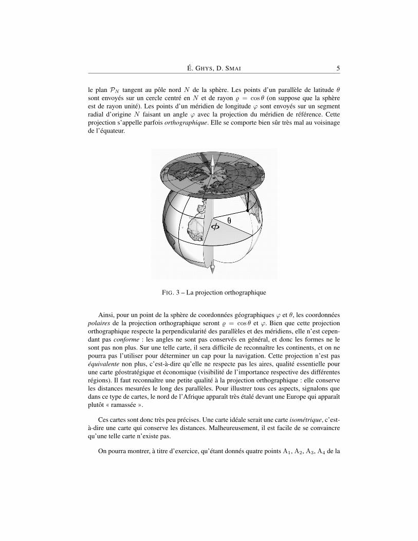
le plan PN tangent au pole nord N de la sphere. Les points d’un parallele de latitude θsont envoyes sur un cercle centre en N et de rayon % = cos θ (on suppose que la sphereest de rayon unite). Les points d’un meridien de longitude ϕ sont envoyes sur un segmentradial d’origine N faisant un angle ϕ avec la projection du meridien de reference. Cetteprojection s’appelle parfois orthographique. Elle se comporte bien sur tres mal au voisinagede l’equateur.
FIG. 3 – La projection orthographique
Ainsi, pour un point de la sphere de coordonnees geographiques ϕ et θ, les coordonneespolaires de la projection orthographique seront % = cos θ et ϕ. Bien que cette projectionorthographique respecte la perpendicularite des paralleles et des meridiens, elle n’est cepen-dant pas conforme : les angles ne sont pas conserves en general, et donc les formes ne lesont pas non plus. Sur une telle carte, il sera difficile de reconnaıtre les continents, et on nepourra pas l’utiliser pour determiner un cap pour la navigation. Cette projection n’est pasequivalente non plus, c’est-a-dire qu’elle ne respecte pas les aires, qualite essentielle pourune carte geostrategique et economique (visibilite de l’importance respective des differentesregions). Il faut reconnaıtre une petite qualite a la projection orthographique : elle conserveles distances mesurees le long des paralleles. Pour illustrer tous ces aspects, signalons quedans ce type de cartes, le nord de l’Afrique apparaıt tres etale devant une Europe qui apparaıtplutot « ramassee ».
Ces cartes sont donc tres peu precises. Une carte ideale serait une carte isometrique, c’est-a-dire une carte qui conserve les distances. Malheureusement, il est facile de se convaincrequ’une telle carte n’existe pas.
On pourra montrer, a titre d’exercice, qu’etant donnes quatre points A1, A2, A3, A4 de la
6 GEOMETRIES ET DYNAMIQUES
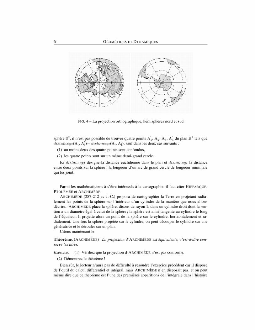
FIG. 4 – La projection orthographique, hemispheres nord et sud
sphere S2, il n’est pas possible de trouver quatre points A′
1, A′
2, A′
3, A′
4 du plan R2 tels quedistanceR2 (A
′
i , A′
j)= distanceS2 (Ai, Aj), sauf dans les deux cas suivants :
(1) au moins deux des quatre points sont confondus,
(2) les quatre points sont sur un meme demi-grand cercle.
Ici distanceR2 designe la distance euclidienne dans le plan et distanceS2 la distanceentre deux points sur la sphere : la longueur d’un arc de grand cercle de longueur minimalequi les joint.
Parmi les mathematiciens a s’etre interesses a la cartographie, il faut citer HIPPARQUE,PTOLEMEE et ARCHIMEDE.
ARCHIMEDE (287-212 av J.-C.) proposa de cartographier la Terre en projetant radia-lement les points de la sphere sur l’interieur d’un cylindre de la maniere que nous allonsdecrire. ARCHIMEDE place la sphere, disons de rayon 1, dans un cylindre droit dont la sec-tion a un diametre egal a celui de la sphere ; la sphere est ainsi tangente au cylindre le longde l’equateur. Il projette alors un point de la sphere sur le cylindre, horizontalement et ra-dialement. Une fois la sphere projetee sur le cylindre, on peut decouper le cylindre sur unegeneratrice et le derouler sur un plan.
Citons maintenant le
Theoreme. (ARCHIMEDE) La projection d’ARCHIMEDE est equivalente, c’est-a-dire con-serve les aires.
Exercice. (1) Verifiez que la projection d’ARCHIMEDE n’est pas conforme.
(2) Demontrez le theoreme !
Bien sur, le lecteur n’aura pas de difficulte a resoudre l’exercice precedent car il disposede l’outil du calcul differentiel et integral, mais ARCHIMEDE n’en disposait pas, et on peutmeme dire que ce theoreme est l’une des premieres apparitions de l’integrale dans l’histoire

E. GHYS, D. SMAI 7
FIG. 5 – Projection d’ARCHIMEDE
FIG. 6 – Projection d’ARCHIMEDE

8 GEOMETRIES ET DYNAMIQUES
des mathematiques. Pour admirer le genie d’ARCHIMEDE, on pourra se plonger dans sesœuvres completes :
http ://www.archive.org/details/worksofarchimede029517mbp.
Cette projection d’ARCHIMEDE s’appelle parfois la projection azimutale equivalente deLambert : ironie de l’histoire.
Avec HIPPARQUE (190–120 av. J.-C.), on commence a s’interesser a la position desetoiles dans le but de les cataloguer. C’est PTOLEMEE (90–170 ap. J.-C.), interesse lui aussipar ce probleme, qui est amene a introduire la celebre projection stereographique.
FIG. 7 – Projection stereographique
On designe par N le pole nord et par E le plan de l’equateur ; le projete d’un point Q dela sphere, different de N , est le point Q′ intersection de la droite NQ avec le plan E . Lesmeridiens sont envoyes sur des demi-droites radiales d’origine O, centre de la sphere, et lesparalleles sur des cercles de centre O. Citons deux theoremes (connus de HIPPARQUE ?) :
Theoreme. (HALLEY, 1656-1743) La projection stereographique envoie un cercle trace surla sphere sur un cercle ou une droite du plan de projection.
Theoreme. La projection stereographique est conforme : deux courbes tracees sur la spherequi se coupent en un point different du pole nord sont projetees sur deux courbes du plan secoupant suivant le meme angle.
Demonstration. La preuve presentee ici est tiree du merveilleux livre de HILBERT et COHN-VOSSEN, intitule The Geometry and the Imagination, dont la lecture est hautement recom-mandee...

E. GHYS, D. SMAI 9
FIG. 8 – Projections stereographiques, centrees aux poles nord et sud
Commencons par la demonstration du second theoreme : la projection est conforme.
NotonsD la droite contenantN,Q,Q′, et PN , PQ les plans tangents a la sphere respecti-vement aux pointsN etQ. Ces plans, pour des raisons de symetrie, forment des angles egauxavec la droite D. Les plans PN et E , etant paralleles, forment des angles egaux avec D.
Soit maintenant ∆ une droite tangente en Q a la sphere. Notons P le plan contenant ∆ etN . Notons enfin ∆′ l’intersection de P avec E .
On deduit des observations precedentes que ∆ et ∆′
forment des angles egaux avec D.Autrement dit, la symetrie par rapport au plan mediateur du segment QQ′ transforme ∆ en∆′.
Si on considere maintenant deux droites ∆1 et ∆2 tangentes en Q, et les deux droites∆′1 et ∆′2 de E qui leur sont associees par le procede precedent, l’angle (non oriente) entreles droites ∆1 et ∆2 est egal a celui entre les droites ∆′1 et ∆′2. En effet, ∆′1 et ∆′2 sont lesimages de ∆1 et ∆2 par une meme symetrie.
Si γ1 et γ2 sont deux courbes tracees sur la sphere et s’intersectant en un pointQ (differentde N ), et si ∆1 et ∆2 designent leurs tangentes respectives en Q, alors les tangentes ∆
′
1 et∆′
2 aux courbes projetees γ′
1 et γ′
2, forment un angle egal a celui des tangentes ∆1 et ∆2.Nous avons donc montre le deuxieme theoreme.
Passons maintenant a la demonstration du premier theoreme : la projection envoie cerclessur cercles.
Soit C un cercle trace sur la sphere et ne passant pas par le pole de la projection N . Lesplans tangents a la sphere en les differents points de C enveloppent un cone de sommet S.La droite NS n’est pas parallele au plan de projection E puisque C ne passe pas par N . SoitS′
le point ou la droite NS intersecte E . Si P est un point de C et P′
son projete sur E , la

10 GEOMETRIES ET DYNAMIQUES
FIG. 9 – Projection stereographique
droite PS est tangente en P a la sphere, et P′S′
est le projete sur E du segment PS. Commeconsequence on a l’egalite des angles P ′PS et PP ′S′ (voir la demonstration precedente).Attention la figure est bien sur vue en perspective si bien que cette egalite ne saute pas auxyeux !
A partir de S tracons la droite parallele a P′S′
et notons P′′
le point ou elle coupeNP
′. Le triangle PP
′′S a des angles en P et P
′′egaux. On a donc SP = SP
′′Observons
maintenant que l’on a P′S′/PS = P
′S′/P′′S = S
′N/SN car les triangles NS
′P′
etNSP
′′sont semblables. On en tire la relation P
′S′
= PS.S′N/SN . On voit ainsi que
lorsque P decrit le cercle C, la longueur du segment PS restant constante, les points P ′
projetes des points P de C restent equidistants de S′. Le projete de C sur E est donc un cercle
de centre S′.
Bien sur, si le cercle C passe par N , la droite intersection du plan du cercle et de E estl’image de C.
Ceci termine la demonstration.
MERCATOR naıt en 1512 et meurt en 1594, epoque ou la navigation maritime connaıt ungrand essor. Il publie le premier livre ou sont collectees des cartes geographiques utiles auxnavigateurs, livre auquel il donne le nom d’Atlas. C’est en 1569 qu’il publie les 18 feuillesde La projection de MERCATOR. La preoccupation majeure des cartographes de cette epoque

E. GHYS, D. SMAI 11
FIG. 10 – La projection stereographique

12 GEOMETRIES ET DYNAMIQUES
etait de concevoir une carte qui transforme les courbes suivies par un marin dont le capest constant, celles qui font un angle constant avec les meridiens, appelees loxodromes, endes droites sur la carte. Pour corriger l’effet de distorsion exageree des regions polaires,notamment celui que donne la projection plate carree, MERCATOR eut l’idee de changerde graduation pour reperer les latitudes. Pour cela il proceda a un changement d’echelles dela forme
(ϕ, θ) 7→ (ϕ, F (θ)).
Et pour resoudre le probleme de la navigation a cap constant il va exiger que ce changementd’echelle soit conforme, ce qui contraint F a verifier l’equation differentielle
dF
dθ=
1cos θ
.
FIG. 11 – La projection de MERCATOR
Bien entendu, MERCATOR ne s’exprime pas de cette maniere et il etait a son epoque im-possible de calculer la primitive de la fonction 1/ cos θ ! Le calcul differentiel n’existait pasencore et meme la fonction logarithme n’avait pas encore ete definie... Ce que faisait MER-CATOR, c’etait en quelque sorte une integration numerique. En tracant sa carte de l’equateurvers le nord, il espacait les paralleles de plus en plus, pour compenser le fait que ceux-ci sonttous representes par des lignes horizontales qui ont toutes la meme longueur sur la carte alorsque sur la sphere, ils sont de plus en plus courts. Cette compensation est faite pour que ladilatation soit la meme dans la direction des meridiens et des paralleles.
Il est a noter que la projection de MERCATOR fausse nos images mentales de la sphere.Dans ces cartes l’Europe occupe par exemple une place plus importante que le nord del’Afrique. On notera aussi que le pole nord est rejete a l’infini (car
∫ π/20
1cos θ dθ =∞).

E. GHYS, D. SMAI 13
Lecon 2 : Cartes optimalesDans ce qui suit, on va s’interesser a la « qualite » des cartes. Un theoreme du a TCHEBY-
CHEV affirme que parmi toutes les cartes conformes d’une region donnee, il en existe une etune seule qui est meilleure que toutes les autres. Mais avant d’en preciser l’enonce, donnonsd’abord des reponses aux questions suivantes :
(1) Qu’est-ce qu’une carte de geographie ?
(2) Qu’appelle-t-on echelle d’une carte ?
(3) Comment mesurer la qualite d’une carte ?
Une carte est une application injective f d’un domaine (i.e. un ouvert connexe) D dela sphere dans le plan R2. Le domaine D est cense representer un pays ou une region de laTerre. Etant donnee une carte f : D → R2, l’echelle de cette carte aux points x, y ∈ D est lerapport
σx,y =distR2(f(x), f(y)distS2(x, y)
.
On notera σ2 = supσx,y l’echelle maximale, σ1 = inf σx,y l’echelle minimale, et onadoptera comme critere de qualite d’une carte le rapport σ2/σ1. Le defaut de la carte seramesure par la quantite positive δ = log(σ2/σ1). La qualite de la carte sera d’autant meilleureque δ est petit, et l’ideal serait que le defaut δ soit nul, ce qui correspondrait a une cartea echelle constante. Un theoreme de MILNOR affirme que pour tout pays D, il existe unecarte optimale, c’est-a-dire une carte f : D → R2 qui minimise le defaut δ(f). Avant dedonner une esquisse de la preuve de cette affirmation signalons une conjecture due egalementa MILNOR (voir : A problem in cartography. Amer. Math. Monthly 76, 1969) :
Conjecture (MILNOR, 1960) SiD est un domaine convexe a l’interieur de l’hemisphere sud(par exemple), alors la carte optimale est unique (a une similitude du plan pres), et c’est undiffeomorphisme sur son image.
On pourrait commencer par s’interesser au cas ou D est un rectangle curviligne delimitepar deux meridiens et deux paralleles pour lequel la carte optimale est inconnue.
Passons maintenant a une esquisse de la preuve de l’affirmation de MILNOR concernantl’existence des cartes optimales.
L’idee est de considerer une suite de cartes fn : D → R2 dont la suite des defauts δ(fn)tend vers la borne inferieure des defauts. On montre ensuite que fn converge vers une cartef∞ dont le defaut est le plus petit possible.
Dans une premiere etape, on centre les cartes en un point p ∈ D en imposant la conditionfn(p) = 0. On suppose que σ2(fn) = 1, quitte a composer les cartes fn avec des similitudesconvenables. Dans une seconde etape, a l’aide du theoreme d’ASCOLI-ARZELA, on extraitune sous-suite (fnk) qui converge. On laisse au lecteur le soin de completer les details.
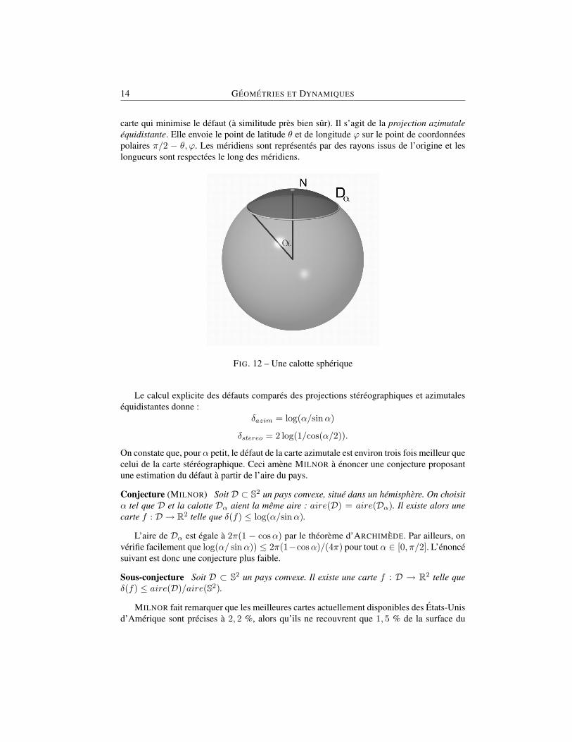
MILNOR considere une calotte spherique Dα dont l’aire est 2π(1 − cosα) (rappelez-vous le theoreme d’Archimede). Il montre que pour un tel domaine, il existe une unique
14 GEOMETRIES ET DYNAMIQUES
carte qui minimise le defaut (a similitude pres bien sur). Il s’agit de la projection azimutaleequidistante. Elle envoie le point de latitude θ et de longitude ϕ sur le point de coordonneespolaires π/2 − θ, ϕ. Les meridiens sont representes par des rayons issus de l’origine et leslongueurs sont respectees le long des meridiens.
FIG. 12 – Une calotte spherique
Le calcul explicite des defauts compares des projections stereographiques et azimutalesequidistantes donne :
δazim = log(α/sinα)
δstereo = 2 log(1/cos(α/2)).
On constate que, pour α petit, le defaut de la carte azimutale est environ trois fois meilleur quecelui de la carte stereographique. Ceci amene MILNOR a enoncer une conjecture proposantune estimation du defaut a partir de l’aire du pays.
Conjecture (MILNOR) Soit D ⊂ S2 un pays convexe, situe dans un hemisphere. On choisitα tel que D et la calotte Dα aient la meme aire : aire(D) = aire(Dα). Il existe alors unecarte f : D → R2 telle que δ(f) ≤ log(α/sinα).
L’aire de Dα est egale a 2π(1 − cosα) par le theoreme d’ARCHIMEDE. Par ailleurs, onverifie facilement que log(α/ sinα)) ≤ 2π(1−cosα)/(4π) pour tout α ∈ [0, π/2]. L’enoncesuivant est donc une conjecture plus faible.
Sous-conjecture Soit D ⊂ S2 un pays convexe. Il existe une carte f : D → R2 telle queδ(f) ≤ aire(D)/aire(S2).
MILNOR fait remarquer que les meilleures cartes actuellement disponibles des Etats-Unisd’Amerique sont precises a 2, 2 %, alors qu’ils ne recouvrent que 1, 5 % de la surface du

E. GHYS, D. SMAI 15
FIG. 13 – Projection azimutale equidistante
FIG. 14 – Projections azimutales equidistantes, centrees aux poles nord et sud

16 GEOMETRIES ET DYNAMIQUES
globe. Le defi est de trouver une carte des Etats-Unis d’Amerique precise a 1, 5 % (meme sice pays n’est pas convexe, ni meme connexe).
Dans toute la discussion que nous venons d’avoir, les cartes ne sont pas necessairementconformes. On peut se poser des questions analogues pour des cartes conformes, et la reponseest alors donnee par un theoreme du a TCHEBYCHEV.
Theoreme. (TCHEBYCHEV) Soit D ⊂ S2 un pays convexe situe dans un hemisphere. Alors,parmi toutes les cartes conformes de D, il en existe une et une seule, a une similitude pres,qui minimise le defaut. Cette carte optimale est caracterisee par le fait que la « dilatation »est constante le long de la frontiere de D.
Precisons ce que l’on entend par conforme. Pour une application R−lineaire L : R2 →R2 avec detL > 0, les proprietes suivantes sont equivalentes :
(1) L respecte les angles : pour tout couple de vecteurs v1, v2, l’angle forme par ces vec-teurs est egal a celui forme par leurs images.
(2) Il existe un reel λ positif tel que pour tout vecteur v, on a ‖Lv‖ = λ‖v‖.
(3) La matrice de L, dans la base canonique de R2, est de la forme(a −bb a
).
(4) Dans l’identification naturelle de R2 a C, l’application L est C-lineaire de C dans C :elle s’ecrit L(v) = µv pour un certain µ de C?.
Une application L qui verifie l’une de ces proprietes est une similitude. Cette notion segeneralise sans difficulte aux applications lineaires entre deux espaces vectoriels de dimen-sion 2 orientes, munis d’une forme quadratique definie positive.
Considerons maintenant deux surfaces orientees S1 et S2, munies des metriques rie-manniennes g1 et g2, si bien que leurs espaces tangents sont munis de formes quadratiquesdefinies positives. Une application f : S1 → S2 est dite conforme si pour tout x dans S1, ladifferentielle dxf est une similitude.
Si f est conforme, il existe donc une application λ : S1 → R?+ telle que l’on ait pour toutx ∈ S1, ‖dxf(v)‖g2 = λ(x)‖v‖g1 .
Remarque. Pour ce qui nous concerne, S1 sera la sphere ronde c’est-a-dire la sphere muniede la metrique induite par la metrique euclidienne de R3.
On appellera dilatation de la carte f au point x le nombre λ(x).
Posons-nous maintenant la question de savoir si une carte conforme est unique au sens oula donnee d’une carte permet de determiner toutes les autres cartes conformes.
Considerons donc deux cartes conformes f et g d’un meme pays D. L’application ϕ =g f−1 est un diffeomorphisme conforme de l’ouvert f(D) sur l’ouvert g(D), et si l’onregarde ces deux ouverts dans C, dire que ϕ est conforme revient a dire que ϕ verifie lesequations de CAUCHY-RIEMANN, c’est-a-dire que ϕ est holomorphe (apres tout, conformeet holomorphe ne sont que deux versions du meme mot, en latin et en grec).
E. GHYS, D. SMAI 17
Resumons : etant donnee une carte conforme f sur D, toute autre carte conforme estobtenue en composant f avec ϕ diffeomorphisme holomorphe entre l’ouvert f(D) et sonimage.
On peut maintenant donner les grandes lignes de la preuve du theoreme de TCHEBY-CHEV.
Pour des raisons de commodite, on inverse le sens des fleches et des applications : unecarte ira d’un ouvert de C vers un pays. Supposons que l’on ait une carte conforme f d’unpays D dont la dilatation soit constante sur la frontiere. Quitte a composer la carte avec unesimilitude, on pourra supposer que la dilatation est egale a 1. Toute autre carte g deD s’ecrirasous la forme g = f ϕ, avec ϕ holomorphe. On se propose alors de montrer que pour toutpoint x on a l’inegalite :
supx
log λg(x)− infx
log λg(x) ≥ supx
log λf (x)− infx
log λf (x),
car ceci entraıne evidemment que le defaut δ(f) de la carte g est superieur a celui de la cartef .
On observe pour cela que :
(1) log λg(x) = log λf (x) + log |ϕ′(f(x))|.
(2) log |ϕ′(x)| est une fonction harmonique ; son maximum et son minimum sont doncatteints sur le bord.
(3) log λf et log λg atteignent leur minimum sur le bord.
(4) log λf ≥ 0 car son minimum est atteint sur le bord et vaut donc 0.
Il reste a montrer qu’il existe effectivement une carte conforme dont la dilatation estegale a 1 sur la frontiere. On considere une carte conforme f dont on suppose la dilatationnon constante sur le bord (par exemple, la projection stereographique), et on la modifie parune fonction holomorphe pour la rendre optimale. La dilatation de la nouvelle carte est :
λf (x)|ϕ′(f(x))|.
Sur f(D) ⊂ C, la fonction log |ϕ′(z)| = < logϕ′(z) est harmonique (noter qu’unedetermination du logarithme existe car on est sur un convexe), et log λf (x) est donne surle bord. La dilatation de la nouvelle carte devant etre constante sur la frontiere, on est alorsamene a trouver une fonction u holomorphe sur f(D) de partie reelle <(u) donnee sur lebord ; c’est le probleme de DIRICHLET pour les fonctions harmoniques. On sait qu’il admetune solution. On obtient ϕ en prenant une primitive de ϕ′(z) = exp(u(z)). L’unicite de lasolution du probleme de DIRICHLET montre alors que la carte conforme optimale est unique.Le theoreme est donc etabli.

18 GEOMETRIES ET DYNAMIQUES
Lecon 3 : Surfaces de RIEMANN
Et si la Terre n’etait pas parfaitement ronde ? En fait, nous savons maintenant que la Terreest presque un ellipsoıde. Existe-t-il encore des cartes conformes ?
C’est GAUSS qui nous repond : il existe toujours une carte conforme sur la Terre, quellequ’en soit la forme.
Avant de donner un enonce precis du theoreme de GAUSS, nous avons besoin de la notionde surface de RIEMANN, notion qui generalise la surface ronde de la Terre que nous avonsdeja consideree.
Definition Une surface de RIEMANN est une surface (variete de dimension 2) munie d’unatlas (Ui, fi), les fi etant des homeomorphismes de Ui vers un ouvert fi(Ui) de C, tel queles changements de cartes
ϕij = fj f−1i : fi(Ui ∩ Uj)→ fj(Ui ∩ Uj)
soient holomorphes.
Remarquons le joyeux anachronisme ! Nous utilisons le nom de RIEMANN dans la de-monstration d’un theoreme de GAUSS... Remarquons egalement l’emploi du mot « atlas »qui remonte, nous l’avons vu, a MERCATOR.
Commencons par un exemple tres simple. La sphere unite peut-etre recouverte par deuxouverts : les complementaires des poles nord et du pole sud, respectivement. Chacun de cesouverts peut etre represente dans le plan R2 ' C par projection stereographique (a partirdes poles nord et sud respectivement). Il n’est pas difficile d’expliciter le « changement decartes » : c’est la transformation z 7→ 1/z qui est une fonction holomorphe. D’ailleurs, iln’est pas necessaire de faire ce calcul pour savoir que le changement de cartes est holomorphepuisque nous savons deja qu’il est conforme. Ainsi, la projection stereographique permet demunir la sphere d’une structure de surface de Riemann ; on parle alors de sphere de RIEMANNC ∪ ∞.Exercice. MERCATOR « invente » le logarithme complexe. Montrer que si on envisage lasphere comme la sphere de RIEMANN, la carte de MERCATOR n’est rien d’autre que l’ap-plication z 7→ log z. Bien sur, il faut decouper le long d’un meridien pour que le logarithmepuisse etre defini sans probleme.
On peut definir la notion de fonction holomorphe entre deux surfaces de Riemann : cesont simplement les fonctions qui sont holomorphes quand on les considere dans les carteslocales. Par exemple, une fonction holomorphe d’un ouvert de C a valeurs dans la spherede RIEMANN C ∪ ∞ est une fonction qui est holomorphe sur l’ouvert ou elle prend desvaleurs finies et dont l’inverse est une fonction holomorphe sur l’ouvert ou elle prend desvaleurs non nulles. On retrouve ainsi le concept de fonctions meromorphes. Retenons doncqu’une fonction holomorphe a valeurs dans la sphere de RIEMANN n’est rien d’autre qu’unefonction meromorphe.

E. GHYS, D. SMAI 19
Signalons qu’une surface de RIEMANN est toujours orientable. Toute surface rieman-nienne orientee, autrement dit, toute surface orientee munie d’une metrique riemanniennedefinit naturellement une surface de RIEMANN grace au theoreme fondamental suivant :
Theoreme. (GAUSS 1822) Soit g une metrique riemannienne sur un ouvert U du plan R2
contenant l’origine. Alors il existe un ouvert V contenant l’origine, et une carte conformeψ : V → ψ(V ) ⊂ R2 ' C.
Rappelons que conforme veut dire qu’il existe une application λ : V → R∗+ telle quepour tout v tangent en x on a gx(v) = λ(x)‖v‖2.
GAUSS a montre ce theoreme sous l’hypothese que g est analytique reelle. Ce theoremefut ensuite demontre dans les cas C∞, C1 (1920), C0 (1960) et meme mesurable.
Une maniere d’exprimer la meme chose consiste a dire qu’une classe conforme de metri-que riemannienne sur une surface definit canoniquement une structure de surface de RIE-MANN. Reciproquement, pour toute surface de RIEMANN, on peut trouver une classe confor-me de metriques riemanniennes qui la definit.
Nous allons donner les grandes lignes de la magnifique demonstration de GAUSS ; onsuppose donc g analytique reelle.
Pour cela, en nous inspirant de la methode de GAUSS, nous allons commencer par de-montrer un theoreme exactement analogue mais dans le cas ou l’ouvert U est muni d’unemetrique lorentzienne g. On se donne donc en chaque point de U une forme quadratiquede signature (+,−) et il s’agit de montrer que cette metrique lorentzienne est conforme a lametrique lorentzienne standard dx2−dy2 de R2 (pour une generalisation evidente du conceptde conformite dans le cadre lorentzien). Voici comment on procede.
En chaque point de U , la metrique g definit deux droites sur lesquelles elle s’annule : lesdeux directions isotropes. Localement, on peut trouver deux champs de vecteurs non singu-liers qui parametrent ces directions. Lorsqu’on les integre, on definit ainsi deux reseaux decourbes isotropes, qui s’intersectent transversalement.
Pour la metrique lorentzienne standard dx2 − dy2, ces courbes ne sont bien entendu queles droites paralleles de pente ±1.
On fixe maintenant un point base p0 dans U et on choisit arbitrairement un point P0 deR2.
Par le point p0 passent deux courbes isotropes C1 et C2. Par P0 passent deux droitesisotropes D1 et D2 de la metrique lorentzienne standard de R2. On envoie C1 sur D1 par undiffeomorphisme f1 arbitraire, et C2 surD2 par un autre diffeomorphisme f2. Soit maintenantun point m de U suffisamment proche de l’origine. Par m passent deux courbes isotropes C1et C2. Quitte a restreindre l’ouvert U en un ouvert plus petit V , on peut supposer que C1intersecte C2 en un seul point p2, et l’autre, C2, intersecte C1 en un seul point p1.
La carte ψ que l’on cherche a construire est celle qui envoie le point m de V sur le pointM = ψ(m) de R2, intersection des droites isotropes de R2 passant par les points P1 = f1(p1)et P2 = f2(p2). La transformation ψ ainsi definie envoie courbes isotropes de V sur droites

20 GEOMETRIES ET DYNAMIQUES
isotropes de R2 et donc directions isotropes de la metrique lorentzienne g sur V sur directionsisotropes de la metrique lorentzienne standard de R2.
Remarquons — c’est un point important — que deux formes quadratiques de signature(+,−) sur un espace vectoriel reel de dimension 2 sont proportionnelles si et seulement sielles ont les memes directions isotropes.
On peut donc ecrire ψ∗g = λ(dx2 − dy2) ou λ est une fonction. Autrement dit ψ est unecarte conforme et le theoreme de GAUSS est etabli dans le cadre lorentzien.
FIG. 15 – Theoreme de GAUSS, version lorentzienne
Dans le cas ou g est une metrique riemannienne analytique reelle, il n’y a bien sur pasde direction isotrope. Mais c’est la meme idee qui est mise en œuvre avec, cependant, plusd’imagination. On commence par complexifier l’ouvert U . Soit donc U ⊂ C2 un complexifiede U ; c’est un voisinage ouvert de U considere maintenant comme contenu dans C2. Onnotera g0 = du2 + dv2 la metrique « riemannienne complexe » standard de C2, u et v etantles fonctions coordonnees usuelles sur C2 (a strictement parler ce n’est pas une metrique rie-mannienne puisque cette forme quadratique prend des valeurs complexes). Les coefficientsde la metrique g etant des fonctions analytiques reelles, on peut les prolonger, de maniereunique, en une metrique g, analytique complexe (i.e. holomorphe) sur l’ouvert U , quitte adiminuer U . Puisque les coefficients de g sont reels, g est invariant par la conjugaison com-plexe (u, v) 7→ (u, v). Sur C2 on dispose de deux reseaux transverses de droites complexesisotropes pour la metrique standard g0, d’equations v = ±iu + cste. Sur U on dispose dedeux champs de droites complexes holomorphes, isotropes pour la metrique g. On integre cesdeux champs pour obtenir deux reseaux de courbes holomorphes se coupant transversalement(ces courbes dans C2 correspondent a des surfaces dans R4).
On fixe maintenant un point p0 dans U et on l’envoie sur un point reel arbitraire P0 deR2 ⊂ C2. Par p0 passe une courbe complexe isotrope C1. Par p0 passe egalement la courbecomplexe C2 transformee par conjugaison complexe de la courbe C1. A l’aide de ces courbeson definit, exactement comme dans le cadre lorentzien, une transformation ψ d’un voisinageV de p0, inclus dans U , a image dans C2, et qui a la propriete additionnelle d’etre invariantepar la conjugaison complexe, ce qui permet de conclure en « decomplexifiant » le cadre quenous avons mis en place. Le fait que la complexification d’un diffeomorphisme ψ preserveles directions isotropes de la complexification d’une metrique signifie precisement que lediffeomorphisme est conforme.
E. GHYS, D. SMAI 21
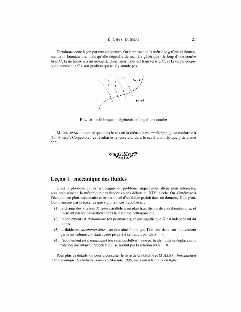
Terminons cette lecon par une conjecture. On suppose que la metrique g n’est ni rieman-nienne ni lorentzienne, mais qu’elle degenere de maniere generique : le long d’une courbelisse C, la metrique g a un noyau de dimension 1 qui est transverse a C, et la valeur proprequi s’annule sur C a son gradient qui ne s’y annule pas.
FIG. 16 – « Metrique » degeneree le long d’une courbe
MIERNOWSKI a montre que dans le cas ou la metrique est analytique, g est conforme adx2 + xdy2. Conjecture : ce resultat est encore vrai dans le cas d’une metrique g de classeC∞.
Lecon 4 : mecanique des fluidesC’est la physique qui est a l’origine du probleme auquel nous allons nous interesser,
plus precisement, la mecanique des fluides en ses debuts au XIXe siecle. On s’interesse al’ecoulement plan stationnaire et irrotationnel d’un fluide parfait dans un domaineD du plan.Commencons par preciser ce que signifient ces hypotheses :
(1) le champ des vitesses X reste parallele a un plan fixe, disons de coordonnees x, y, etinvariant par les translations dans la direction orthogonale z.
(2) l’ecoulement est stationnaire (ou permanent), ce qui signifie que X est independant dutemps.
(3) le fluide est incompressible : un domaine fluide que l’on suit dans son mouvementgarde un volume constant ; cette propriete se traduit par divX = 0.
(4) l’ecoulement est irrotationnel (ou sans tourbillon) : une particule fluide se deplace sansrotation instantanee, propriete qui se traduit par la relation rotX = 0.
Pour plus de details, on pourra consulter le livre de GERMAIN et MULLER : Introductiona la mecanique des milieux continus, Masson, 1995, mais aussi le cours en ligne :

22 GEOMETRIES ET DYNAMIQUES
www.diam.unige.it/∼irro/elementari e.html, ouwww.eng.fsu.edu/dommelen/courses/flm/flm00/topics/pot/index.html.
Sur D on definit deux 1-formes differentielles, ω et ω?, en posant pour tout v ∈ R2
ω(v) =< v,X > et ω?(v) =< v,X⊥ >,
ou <,> designe le produit scalaire et X⊥ est le vecteur X tourne de 90 degres dans le senscontraire des aiguilles d’une montre ; si X a pour composantes X1 et X2 dans un systeme decoordonnees orthonormees, X⊥ a pour composantes X2 et −X1. Les differentielles de ω etω? s’ecrivent respectivement :
dω = (rotX)dx ∧ dy et dω? = (divX)dx ∧ dy.
Les hypotheses (3) et (4) se traduisent alors par les relations (3′) : dω? = 0 et (4′) :dω = 0. On regroupe ω et ω? en une seule forme differentielle complexe Ω en posant Ω =ω − iω?. En fait Ω est C-lineaire si bien que Ω est une 1-forme complexe fermee : dΩ = 0.Il existe donc une fonction f , holomorphe sur D, telle que Ω = f(z) dz avec z = x +iy. Cette fonction est appelee, selon une terminologie en usage chez les mecaniciens desfluides, vitesse complexe (improprement sans doute car il s’agit en fait de la vitesse complexeconjuguee). On peut donc dire, dans la situation la plus generale « qu’un ecoulement est unefonction holomorphe ». En integrant f (au moins localement) on peut ecrire Ω = dΦ, avec Φholomorphe. La fonction Φ est le potentiel (complexe) de l’ecoulement.
La transformation Φ envoie les lignes de courant (orbites du champX) qui sont egalementles trajectoires des particules fluides (puisque l’ecoulement est stationnaire) sur les droiteshorizontales <(w) = cste. Les lignes de courant sont les lignes de niveau de la partie imagi-naire de Φ. La connaissance de Φ determine entierement l’ecoulement. En notant X1 et X2
les composantes du vecteur X , on a les egalites
X = X1 − iX2 = f =dΦdz,
Voici quelques exemples d’ecoulement.
(1) ecoulement uniforme : f(z) = 1 et Φ(z) = z.
FIG. 17 – Un flot constant
Le champ des vitesses X est constant.

E. GHYS, D. SMAI 23
(2) Robinet (source) Siphon(puits)Φ(z) = log z, Φ(z) = − log z,f(z) = 1/z, f(z) = −1/z,X = 1/z, X = −1/z,.
FIG. 18 – Une source
Ces potentiels definissent des ecoulements dans tout le plan prive de l’origine.
(3) Vortex ou tourbillonΦ(z) = i log z,f(z) = i/z,X(z) = −i/z.
FIG. 19 – Un tourbillon
L’ecoulement est defini sur C?, invariant par rotations.
(4) Ecoulement autour d’un disqueΦ(z) = z + 1/z,f(z) = 1− 1/z2,X(z) = 1− 1/z2.Cet ecoulement est celui qui s’etablit autour d’un disque (de rayon unite et centre en 0)place dans un ecoulement uniforme.
Apres avoir fait connaissance avec quelques types d’ecoulements, nous allons a presentcalculer la resultante des efforts exerces sur un obstacle plonge dans un fluide en ecoulement.Considerons un ecoulement stationnaire et irrotationnel autour d’un obstacle cylindrique,

24 GEOMETRIES ET DYNAMIQUES
FIG. 20 – Un flot autour d’un cercle
a section quelconque, qu’on supposera infiniment long, ce qui nous autorisera a supposerl’ecoulement plan, de direction orthogonale aux generatrices de l’obstacle. La situation ty-pique est celle d’une aile d’un avion volant a une vitesse constante −V∞. Pour les vitesses(tres) inferieures a la vitesse du son, l’air peut etre assimile a un fluide incompressible eton peut negliger les tourbillons autour de l’aile (pas tres realiste en fait...). Pour des raisonsde commodite on supposera que c’est l’obstacle qui est immobile et que les filets de fluideglissent sur l’obstacle avec une vitesse constante V∞ a l’infini.
Il s’agit de calculer les efforts (par unite de longueur dans la direction orthogonale duplan de l’ecoulement). Considerons donc une portion cylindrique Σ comprise entre deuxplans paralleles distants l’un de l’autre d’une longueur unite. Appelons C la courbe fermeeprojection de Σ sur le plan x, y, plan de l’ecoulement. Le fluide etant suppose parfait, laresultante R des efforts exerces sur la paroi Σ est perpendiculaire a Σ ; ces efforts sont desefforts de pression et sont donnes par l’integrale
R = −∫
P p n dσ
ou p represente la pression par unite de surface, et ou n designe le vecteur unitaire normal aΣ dirige vers l’exterieur de l’obstacle. Si dans le plan des x, y on parametre C (orientee dansle sens contraire des aiguilles d’une montre) par sa longueur d’arc s, alors
(x(s), y(s), ξ
),
s ∈ [0, l] est une parametrisation de Σ (ξ ∈ [0, 1] designe la troisieme composante usuelle deR3). L’element d’aire dσ sur Σ est ds dξ. On peut alors ecrire
R = −∫ l
0
pn ds.
Pour tirer profit des proprietes des fonctions holomorphes on calculera R = Rx − iRy , ennotant Rx et Ry etant les composantes de R suivant les axes des x et des y respectivement.Or n = −idzds de sorte que
R = −∫ l
0
pn ds = −i∫C
p dz.

E. GHYS, D. SMAI 25
La pression est donnee par la loi de BERNOULLI, loi selon laquelle, pour un ecoulementpermanent et irrotationnel, la quantite ρ
2 |X|2 + p reste constante dans tout le fluide et dans
le temps (ou ρ designe la masse volumique du fluide). Ce nombre est la somme de l’energiecinetique et d’une energie potentielle associee aux forces de pression. On aura donc, apresavoir note A cette constante :
R = −i∫C
pdz = −∫C
(A− ρ
2|X|2
)dz = i
ρ
2
∫C
|X|2dz,
soit :R = i
ρ
2
∫C
ffdz.
Notons ϕ = <Φ et ψ = =Φ. Sur C, on a dψ = 0, car C est une ligne de courant etles particules fluides glissent sur le bord de l’obstacle et n’y adherent pas (c’est la conditionsur le bord pour l’ecoulement d’un fluide parfait), et que l’ecoulement est permanent. DoncdΦ = dϕ+ idψ est reelle sur C. Or dΦ = fdz de sorte que
R = iρ
2
∫C
f2dz.
Ecrivons la vitesse complexe f(z) sous forme d’un developpement au voisinage de l’infini(loin de l’obstacle l’ecoulement est presque uniforme et parallele a l’axe des x, de vitesseV∞) :
f(z) = V∞ +C−1
z+C−2
z2+ · · ·
Il vient donc :f2(z) = V 2
∞ + 2C−1V∞1z
+ · · ·
d’ouR = −2ρπC−1V∞.
Introduisons la circulation du champ des vitesses le long de C definie par
Γ =∫C
f(z) dz = 2iπC−1.
Ce nombre Γ est reel car f(z)dz est reel le long de C ; il peut etre non nul, bien quel’ecoulement soit irrotationnel, et ceci n’est pas contradictoire car le domaine occupe parl’obstacle est un « trou » de bordC dans le domaine de l’ecoulement. En ecrivantRx−iRy =−2iΓV∞, on en deduit :
R = ρΓV∞i.
C’est la formule de BLASIUS ; elle permet de determiner tres simplement les efforts glo-baux exerces par le fluide sur le profil de l’obstacle.
Il est a noter que R est de direction perpendiculaire a celle de l’ecoulement a l’infini.C’est le fameux paradoxe de D’ALEMBERT qui contredit l’experience la plus commune : lefluide n’exerce aucune force de trainee... Cette forceR, lorsqu’elle est non nulle, c’est-a-direlorsque Γ est non nul, est appelee force de portance, et s’exerce vers le haut si Γ > 0. Lorsque
26 GEOMETRIES ET DYNAMIQUES
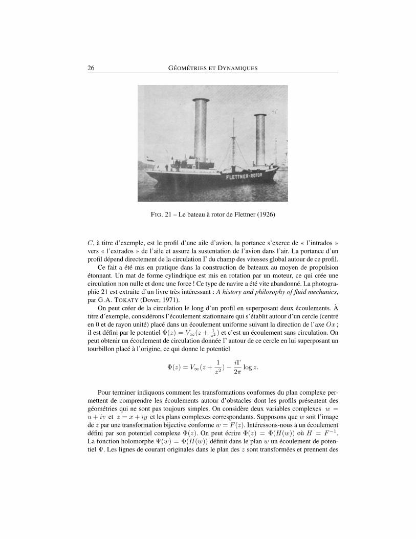
FIG. 21 – Le bateau a rotor de Flettner (1926)
C, a titre d’exemple, est le profil d’une aile d’avion, la portance s’exerce de « l’intrados »vers « l’extrados » de l’aile et assure la sustentation de l’avion dans l’air. La portance d’unprofil depend directement de la circulation Γ du champ des vitesses global autour de ce profil.
Ce fait a ete mis en pratique dans la construction de bateaux au moyen de propulsionetonnant. Un mat de forme cylindrique est mis en rotation par un moteur, ce qui cree unecirculation non nulle et donc une force ! Ce type de navire a ete vite abandonne. La photogra-phie 21 est extraite d’un livre tres interessant : A history and philosophy of fluid mechanics,par G.A. TOKATY (Dover, 1971).
On peut creer de la circulation le long d’un profil en superposant deux ecoulements. Atitre d’exemple, considerons l’ecoulement stationnaire qui s’etablit autour d’un cercle (centreen 0 et de rayon unite) place dans un ecoulement uniforme suivant la direction de l’axe Ox ;il est defini par le potentiel Φ(z) = V∞(z + 1
z2 ) et c’est un ecoulement sans circulation. Onpeut obtenir un ecoulement de circulation donnee Γ autour de ce cercle en lui superposant untourbillon place a l’origine, ce qui donne le potentiel
Φ(z) = V∞(z +1z2
)− iΓ2π
log z.
Pour terminer indiquons comment les transformations conformes du plan complexe per-mettent de comprendre les ecoulements autour d’obstacles dont les profils presentent desgeometries qui ne sont pas toujours simples. On considere deux variables complexes w =u+ iv et z = x+ iy et les plans complexes correspondants. Supposons que w soit l’imagede z par une transformation bijective conforme w = F (z). Interessons-nous a un ecoulementdefini par son potentiel complexe Φ(z). On peut ecrire Φ(z) = Φ(H(w)) ou H = F−1.La fonction holomorphe Ψ(w) = Φ(H(w)) definit dans le plan w un ecoulement de poten-tiel Ψ. Les lignes de courant originales dans le plan des z sont transformees et prennent des

E. GHYS, D. SMAI 27
FIG. 22 – Un flot autour d’un cercle, avec circulation non nulle
formes differentes dans le plan des w. Ainsi un ecoulement stationnaire, incompressible etirrotationnel autour d’un profil dans le plan des z equivaut a un ecoulement ayant les memesproprietes dans le plan des w autour d’un profil de geometrie differente. La vitesse complexedans le plan w est donnee par
g(w) =dΨdw
=dΦdz
dH
dw=
f(z)F ′(z)
.
Notons que la transformation F ne change pas la circulation autour du profil. En effet :∫Cw
g(w)dw =∫Cz
f(z)F ′(z)
dw =∫Cz
f(z)dz.
Signalons, pour illustrer cette demarche, que JOUKOWSKY a remarque que la transfor-mation w = F (z) = z + 1
z transforme des cercles bien choisis en des contours qui peuventrepresenter un profil d’aile d’avion. En comprenant l’ecoulement d’un fluide autour d’uncercle on peut donc comprendre l’ecoulement autour de certaines ailes d’avion. Bien sur, toutceci a surtout un interet historique car les hypotheses que nous avons faites sont bien loin dela realite physique. Pour quelques details sur l’aerodynamique « appliquee » dans un contexteplus realiste, on pourra consulter le « digital textbook »
www.desktopaero.com/appliedaero/preface/welcome.html.

28 GEOMETRIES ET DYNAMIQUES
FIG. 23 – Une aile de Joukowsky
Lecon 5 : le theoreme de RIEMANN-ROCH
Le but de cette lecon est une presentation du theoreme de RIEMANN-ROCH. On peut direque ce theoreme apporte une reponse a un probleme dont l’origine remonte a la physique duXIXeme siecle a travers l’etude du mouvement des fluides.
Dans la lecon precedente nous avons vu comment un ecoulement plan sans source (oupuits) ni tourbillon est entierement caracterise par une forme differentielle holomorphe Ω,exacte (au moins localement, sans hypothese sur la topologie globale du domaine de l’ecou-lement). En ecrivant Ω = dΦ = fdz, avec Φ et f holomorphes, on a le potentiel com-plexe ainsi que le champ des vitesses X = f(z) de l’ecoulement. Inversement etant donneeune forme holomorphe Ω = fdz, on peut interpreter f comme la vitesse complexe d’unecoulement plan irrotationnel d’un fluide parfait incompressible. Localement, le potentielcomplexe de l’ecoulement est donne par une primitive de f . Nous pouvons ainsi dire qu’unecoulement plan irrotationnel d’un fluide parfait incompressible est une 1-forme holomorphe,avec a notre disposition, un dictionnaire physico-mathematique permettant le passage d’unelecture a l’autre.
Signalons avant de clore ces propos, que si le domaine de l’ecoulement est multiple-ment connexe (presence de trous) – et c’est notamment le cas lorsqu’il y a des « robinetsponctuels » (sources et puits) qui correspondent a des points du plan ou divX 6= 0, ou destourbillons qui correspondent aux points ou rotX 6= 0 (au sens des distributions) – il faut ex-clure ces points du domaine pour que notre construction soit possible. L’integration de f faitalors apparaıtre des constantes cycliques (ou periodes) correspondant aux debits des robinetset aux intensites des tourbillons, et le potentiel complexe de l’ecoulement sera une fonctionmultiforme.

E. GHYS, D. SMAI 29
Interessons-nous maintenant a l’ecoulement d’un fluide ideal incompressible sur une sur-face de RIEMANN Σ. On voudrait evidemment reconduire sur Σ la construction de la 1-formeΩ qui caracterise un ecoulement plan. Or pour ecrire la divergence ou le rotationnel d’unchamp de vecteurs sur une variete, on a besoin d’une metrique riemannienne. Comment choi-sir alors une metrique g sur Σ ? Il faudrait que la structure complexe de Σ (structure de surfacede RIEMANN) soit compatible avec la structure conforme induite par le choix de g. Precisonscette notion de compatibilite : si g est une metrique sur Σ nous avons appris que (Σ, g) estlocalement conformement plate c’est-a-dire qu’il existe au voisinage de chaque point de Σune carte (U,ϕ) telle que ϕ?g = λ (dx2 + dy2) ou λ est une fonction reguliere sur U . L’atlas(U,ϕ) definit alors une structure de surface de RIEMANN sur Σ. Nous savons egalementque deux metriques conformement equivalentes definissent la meme structure de surface deRIEMANN sur Σ. Plus precisement on a une correspondance biunivoque :
structures de surface de RIEMANN sur Σ, classes conformes decompatibles avec sa structure de ←→ metriques riemanniennessurface reelle C∞ sur Σ et orientation de Σ.
Soit donc g une metrique qui induit la structure de surface de RIEMANN de Σ, et X lechamp des vitesses d’un ecoulement sur Σ. On verifie alors immediatement que si X⊥ estorthogonal a X et de meme longueur pour la metrique g, alors e−uX⊥ est orthogonal a X etde meme longueur pour la metrique g = eug. En revanche, la forme Ω ne change pas ; ellene depend que de la classe conforme de g. Ainsi, sur une surface de RIEMANN, l’objet quicaracterise l’ecoulement et qui possede un statut intrinseque est la 1-forme holomorphe Ω.
Pour commencer, voyons comment on pourrait faire couler un fluide, de l’eau par exem-ple, sur la sphere S2. La sphere, c’est le plan complexe C plus un point a l’infini. Il suffit alorsde placer un robinet a l’origine, de l’ouvrir, de regler son debit a 2π et de laisser couler. La1-forme de cet ecoulement est Ω = dz
z qu’on peut integrer localement pour avoir le potentielΦ(z) = log z.
A l’aide de la projection stereographique par rapport au pole nord N , on remonte l’ecou-lement sur la sphere : on obtient alors un ecoulement qui part du pole sud et qui va vers lepole nord. Le potentiel de cet ecoulement n’est rien d’autre que la projection de MERCATORqui envoie paralleles sur horizontales et meridiens sur verticales. On uniformise ce potentielen procedant a une coupure sur la sphere le long d’un meridien par exemple.
Si l’on part d’un ecoulement dans le plan complexe obtenu par superposition d’une sourceet d’un tourbillon a l’origine, les lignes de courant, dans le plan de l’ecoulement, sont desspirales logarithmiques. Lorsqu’on remonte cet ecoulement sur la sphere a l’aide de la pro-jection stereographique, les lignes de courant sont des loxodromes. Le potentiel est donne parla 1-forme Ω + Ω? avec Ω? = idzz .
Enoncons maintenant un theoreme :
Theoreme. (RIEMANN) Sur toute surface de RIEMANN compacte Σ, il existe une fonctionmeromorphe non constante f : Σ→ C ∪ ∞.
30 GEOMETRIES ET DYNAMIQUES
Il n’est malheureusement pas question de donner une preuve ici. Les preuves completessont delicates. F. KLEIN a essaye de reconstruire les intuitions physiques qui ont pu guiderRIEMANN dans l’elaboration de ce type de theoreme. On consultera avec profit le petit livrede KLEIN : On RIEMANN’s theory of algebraic functions and their integrals. A suplement tothe usual treatises. Dover Publications, Inc., New York, 1963. Nous allons essayer de suivrece genre d’idees qui ne sont absolument pas des demonstrations mais qui peuvent nourrirl’intuition.
« Preuve »F. KLEIN propose de construire la differentielle de f au lieu de f elle-meme. Pour etre
plus precis, on cherche une 1-forme meromorphe Ω sur Σ qui, sous certaines conditions,admettra une primitive globale f sur Σ. Cette forme sera obtenue comme la 1-forme ca-racterisant un ecoulement sur Σ. En ouvrant des robinets en quelques points de Σ et enlaissant couler on provoque un ecoulement sur Σ, et on espere arriver ainsi a une solutionphysique du probleme dont la traduction mathematique nous donnera la fonction f cherchee.
Commencons par examiner s’il est possible de faire couler de l’eau sur une sphere sansouvrir de robinets ni tourbillons. La sphere etant simplement connexe la forme fermee Ω estexacte : il existe une fonction f sur Σ, holomorphe telle que Ω = df . Mais Σ etant compacteet f etant holomorphe, f est constante (par le principe du maximum). La reponse est doncnegative.
Sur le tore C/(Z+iZ) par contre, un tel ecoulement est possible. Il existe, a une constantecomplexe multiplicative pres, une unique forme differentielle holomorphe dz. Il s’agit del’ecoulement uniforme le long des meridiens ou des paralleles (on passe de l’un a l’autre parla multiplication par i).
Placons nous maintenant sur une surface de RIEMANN Σ de genre g superieur ou egal a2. La encore, la reponse est positive.
On dit que deux courbes fermees γ, γ′ sur une surface Σ sont homologues s’il existe unesurface orientee Z dont le bord ∂Z est constitue de deux cercles orientes, et une applicationi : Z → Σ dont la restriction aux deux composantes de bord definit γ, γ′. Une applicationsimple de la formule de STOKES montre que le flux du champ des vitessesX d’un ecoulementΩ a travers deux courbes homologues γ et γ′ ne change pas : Flux(X, γ′) = Flux(X, γ) =<(∫γ
Ω).Il y a 2g courbes γi qui « captent » l’homologie de Σ, a savoir g « meridiens » et g « pa-
ralleles ». Si on se donne 2g flux, a travers les courbes γi il existe un ecoulement unique sur Σqui realise ces flux. Ceci n’est que la traduction hydrodynamique du theoreme mathematiquesuivant.
Theoreme. (ABEL) Etant donnes 2g nombres reels α1, α2, ..., α2g il existe une unique1-forme holomorphe Ω sur Σ telle que l’on ait <(
∫γi
Ω) = αi.
Autrement dit, la dimension reelle (resp. complexe) de l’espace des 1-formes holomor-phes sur Σ est 2g (resp.g). Pour aller vers une solution de notre probleme initial, construiredes fonctions meromorphes, on va placer k robinets en k points x1, x2..., xk de Σ que l’onaffecte respectivement des nombres complexes λ1, λ2..., λk :

E. GHYS, D. SMAI 31
FIG. 24 – Deux courbes homologues sur une surface de genre 3
FIG. 25 – Une base de l’homologie

32 GEOMETRIES ET DYNAMIQUES
• <(λi) > 0 si de l’eau sort de xi,• <(λi) < 0 si de l’eau est absorbee en xi,• =λi est non nul si l’eau tourbillonne autour de xi.La partie reelle de λi represente, a un coefficient multiplicatif pres, le debit sortant a
travers un contour qui entoure le point xi une fois. La partie imaginaire de λi represente lacirculation le long d’une courbe qui entoure une fois le point xi. Pour qu’un tel ecoulementexiste, la physique nous impose d’ecrire que le bilan est nul ; la quantite d’eau qui sort desrobinets est egale a la quantite d’eau absorbee, et la circulation totale autour de tous les xi estnulle. La condition necessaire que l’on doit ecrire est donc Σλi = 0.
Theoreme. Sous cette derniere condition, il existe sur Σ un unique ecoulement ayant lescaracteristiques voulues (flux, debits et circulations donnes).
« Preuve ». On met sur Σ un ecoulement qui realise les flux (c’est assure par le theoremeprecedent). Puis on choisit k points sur Σ en lesquels on place des robinets et des tourbillons.On ouvre et on laisse couler... On obtient ainsi l’ecoulement recherche (qui est en fait lasuperposition de k + 1 ecoulements).
Localement, au voisinage de xi, la forme Ω s’ecrit Ω =(λi/z + h(z)
)dz avec h ho-
lomorphe. N’oublions pas que, suivant l’idee de RIEMANN, ce que nous voulons, c’est uneforme meromorphe dont la primitive est une fonction meromorphe. Il nous faut donc integrerΩ, et la nous essuyons un echec puisque la primitive de 1/z n’est pas une fonction uniforme.On y remedie en placant des dipoles hydrodynamiques a la place des robinets. Un dipolehydrodynamique est la limite de l’ecoulement resultant de la superposition d’un robinet adebit positif (source) et d’un robinet a debit negatif (puits). Voici comment on le fabrique : onplace une source de debit D en un point A d’affixe a reel, et un puits de debit −D au pointA′ d’affixe −a ; l’ecoulement qui resulte de leur superposition a pour potentiel complexe lafonction
Φ(z) =D
2πlog
z − az + a
qui est uniforme dans le plan prive du segment [A,A′]. Les lignes de courant sont des arcs decercles passant parA etA′. Notons que le bilan pour ce dipole est nul : ce qui sort est aussitotrejete.
FIG. 26 – Un puits et une source proches

E. GHYS, D. SMAI 33
Posons 2aD = K et faisant tendre a vers 0 tout en maintenant K fixe (necessairementD tend vers l’infini). L’ecoulement defini par Φ tend alors vers l’ecoulement du dipole hy-drodynamique place en O, d’axe Ox et de moment K, dont le potentiel est Φ(z) = − K
2πz .Pour ce dipole hydrodynamique Ω = λdzz2 avec K = 2πλ.
FIG. 27 – Un dipole
On peut donc enoncer le theoreme suivant :
Theoreme. Etant donnes 2g flux αi a travers les courbes γi, et k moments dipolairesλ1, ..., λk, il existe un unique flot X avec ces caracteristiques.
« Preuve ». On met sur Σ un flot qui realise les flux et on lui superpose les flots de k dipoleshydrodynamiques places en k points x1, ..., xk.
Passons maintenant a la « demonstration » du theoreme de RIEMANN-ROCH proprementdit. Pour un ecoulement donne par le theoreme precedent, la forme Ω qui le code s’ecritlocalement, dans un voisinage d’un dipole xi, sous la forme Ω =
(λiz2 + h(z)
)dz, avec h
holomorphe.
On voudrait en prendre une primitive f , par integration le long d’un chemin joignant unpoint x0 fixe sur Σ a un point variable z de Σ. On pose donc f(z) =
∫ zx0
Ω. Pour que cettedefinition soit correcte, il faudrait que
∫γ
Ω = 0 pour toute courbe fermee γ. Tout cycle γest homologue a une combinaison lineaire a coefficients entiers des 2g cycles basiques γi deΣ. La forme Ω est une combinaison lineaire a coefficients complexes a1Ω1 + ... + akΩk +C1ω1 + ... + Cgωg , ou les formes ωi constituent une base sur C de l’espace des formesholomorphes sur Σ, et ou les formes Ωi caracterisent les dipoles. En ecrivant que l’on doitavoir
∫γi
Ω = 0 pour chaque i, pour pouvoir integrer globalement Ω, on obtient un systemelineaire de 2p equations a p + k inconnues, les coefficients ai et Ci. Ce systeme possedeune solution non triviale des que p + k > 2p. On peut donc enoncer ainsi le theoreme deRiemann-Roch « comme un mecanicien des fluides ».
Theoreme. Si on place plus de dipoles que le genre sur la surface, on a une solution a notreprobleme.

34 GEOMETRIES ET DYNAMIQUES
L’interpretation mathematique de ce dernier theoreme est le theoreme de RIEMANN-ROCH pour une surface de RIEMANN.
Theoreme. (RIEMANN-ROCH) Soit Σ une surface de RIEMANN de genre g. Si k > g, alors,il existe sur Σ une forme differentielle meromorphe non triviale Ω qui est exacte, et dont laprimitive f est une fonction meromorphe sur Σ possedant k poles.
Lecon 6 : Geometrie analytique, Geometrie algebriqueOn se propose dans cette lecon de montrer que surfaces de RIEMANN et les courbes
algebriques ne sont que deux manieres d’apprehender un meme objet geometrique. Les « de-monstrations » seront encore plus imprecises que dans les lecons precedentes.
Theoreme. (RIEMANN) (1) Une surface de RIEMANN compacte « est » une courbe alge-brique.
(2) Une courbe algebrique « est » une surface de RIEMANN compacte.
En termes quelque peu abstraits, ce theoreme met en bijection des objets algebriques etdes objets analytiques. On a la le premier exemple d’un resultat qui illustre les liens profondsentre la geometrie algebrique et la geometrie analytique, et connus sous le nom de « prin-cipe GAGA », en reference a l’article celebre de SERRE intitule « Geometrie Algebrique etGeometrie Analytique » : « un objet analytique global sur une variete projective est alge-brique ».
Commencons par expliciter une remarque tres simple mais qui sera fondamentale. Lesfonctions holomorphes de la sphere de RIEMANN C∪∞ dans elle-meme sont des fonctionsmeromorphes de la variable z ∈ C qui sont egalement meromorphes a l’infini dans le sensque ce sont des fonctions meromorphes de la variable 1/z. Il est bien connu que ce sontles fractions rationnelles de la variable z. Ainsi les fonctions holomorphes de la sphere deRIEMANN dans elle-meme ne sont autres que les fractions rationnelles. Voila un premierexemple montrant que certaines fonctions holomophes sont necessairement « algebriques ».
Une courbe algebrique (affine) C est le lieu des zeros dans C2, d’un polynome P nonconstant de C[X,Y ] :
C = (x, y) ∈ C2 : P (x, y) = 0.
Il s’agit donc d’une courbe complexe dans C2, objet geometrique de dimension complexe 1.Dans un environnement reelC est definie par deux equations :<P = 0 et=P = 0. La courbeC nous y apparaıt donc comme un objet geometrique a deux dimensions reelles, c’est-a-direcomme une surface.

E. GHYS, D. SMAI 35
Commencons par donner les grandes lignes de la demonstration de l’affirmation 2 dutheoreme. Il s’agit de definir une structure de surface de RIEMANN sur l’ensemble des zerosd’un polynome. L’idee est que C est localement, la ou elle est non singuliere, un graphe audessus de sa tangente (droite complexe de C2). On pourra alors parametrer un petit ouvertde C par un petit ouvert de tangente. Il n’est pas difficile de s’assurer que ces cartes localesdefinissent bien une structure de surface de RIEMANN. Lorsque la courbe est non singuliere,elle definit donc bien une surface de RIEMANN. Cette surface n’est pas compacte et il faut la« compactifier ». La methode la plus simple consiste a « rendre le polynome P homogene ».Si d designe le degre de P , on pose :
P (x, y, z) = zdP (x/z, y/z)
si bien que P est maintenant un polynome homogene de degre d en trois variables dont le lieudes zeros est un cone dans C3 qui definit donc une partie du plan projectif complexe CP2 ;c’est la courbe projective associee a P . Dans la « carte affine » ou z est non nul, cet ensembles’identifie au lieu des zeros de P . Dans les autres cartes affines, par exemple la ou x ou y estnon nul, il s’identifie au lieu des zeros d’un autre polynome. Lorsque la courbe projective estnon singuliere, elle definit une surface de RIEMANN compacte.
Disons maintenant quelques mots du cas ou la courbe projective presente des singula-rites. Tout d’abord les singularites d’une courbe irreductible de C2 sont isolees. Si l’on nes’interesse pas a la structure de la singularite, la question se pose de savoir comment la « sup-primer », ou, selon la terminologie consacree, comment la « resoudre ». Il s’agit de montrerqu’il existe une surface de RIEMANN compacte C telle que C privee de ses points singuliersest isomorphe, comme surface de RIEMANN, a C privee d’un nombre fini de points. Il y abeaucoup de methodes pour atteindre ce but, comme par exemple celle qui consiste a eclaterles points singuliers un nombre suffisant de fois...
On montre maintenant que par la construction que nous venons d’esquisser on retrouvetoutes les surfaces de RIEMANN compactes. Plus precisement on montre que toute surfacede RIEMANN compacte « abstraite » peut etre representee comme une courbe algebriqueprojective (comprendre par la qu’elle est isomorphe a la surface de RIEMANN associee acette courbe, et que deux surfaces de RIEMANN sont isomorphes s’il existe entre elles uneapplication bijective biholomorphe).
Soit Σ une surface de RIEMANN compacte. Le theoreme de RIEMANN-ROCH nous assureque l’on peut trouver deux fonctions meromorphes non constantes sur Σ, donc deux fonctionsholomorphes non constantes f1, f2 : Σ → C = C ∪ ∞. En dimension 1 complexe, Σ estune courbe et son image par (f1, f2) est une courbe C de C2. Cette courbe est algebrique !Voici comment on le montre. L’idee de depart consiste a couper C par une verticale x × Cpuis de construire astucieusement, a l’aide des ordonnees des points d’intersection, une fonc-tion holomorphe de C dans C. La courbe C est parametree par les points de Σ : (x, y) ∈ C siet seulement si x = f1(p) et y = f2(p) pour un p ∈ Σ. La fonction non constante f1 : Σ→ Cetant meromorphe il se trouve que, sauf pour un nombre fini de points x1, ..., xk de C, la fibref−1
1 (x) au dessus de x, contient toujours le meme nombre r d’elements de Σ. Soit donc
36 GEOMETRIES ET DYNAMIQUES
x ∈ C− x1, ..., xr. Posons f−11 (x) = s1(x), ..., sr(x). On prendra garde au fait que les
si en tant que « fonctions » de x sont mal definies, c’est-a-dire sont multiformes. L’ensembles1(x), ..., sr(x) est bien defini mais il n’est pas possible d’ordonner ses elements pour for-mer r fonctions holomorphes. Les ordonnees des r points ou la droite x× C coupe C sontdonnees par yi(x) = f2(si(x)), i variant de 1 a r. La encore on a ainsi r « fonctions » yimultiformes sur C− x1, ..., xk ;
Pour aller plus loin, supposons dans un premier temps que chaque verticale x×C coupeC en un point unique y1(x) (r = 1). On a ainsi une application holomorphe y1 : C → C.Cette application y1 est donc une fraction rationnelle et on peut ecrire y1(x) = A(x)/B(x)avec A,B ∈ C[X]. Observons maintenant que le couple (x, y) ∈ C × C est un point de Csi et seulement si y = y1(x). Posons alors F (x, y) = yB(x) − A(x) de sorte que F est unpolynome en les variables x et y, a coefficients complexes et on a F (f1, f2) = 0. La surfacede RIEMANN associee a la courbe C est isomorphe a Σ si bien que la surface de RIEMANNC est bien associee a une courbe algebrique.
Supposons maintenant que chaque verticale x × C coupe C en deux points y1(x) ety2(x) (r = 2). Comme il n’y a pas d’ordre sur C, on ne peut considerer separement cesdeux points. Les « fonctions » y1 et y2 sont donc multiformes. Par contre leur somme etleur produit, σ(x) = y1(x) + y2(x) et ρ(x) = y1(x)y2(x) sont bien definis car ce sont desfonctions symetriques. Ces applications sont holomorphes de C dans C, donc des fractionsrationnelles :
σ(x) = A1(x)/B1(x) ; ρ(x) = A2(x)/B2(x).
Elles sont solutions de l’equation du second degre :
y2 − A1(x)B1(x)
y +A2(x)B2(x)
= 0.
On termine alors comme precedemment ; si on pose :
F (x, y) =(y2 − A1(x)
B1(x)y +
A2(x)B2(x)
)B2(x)B1(x),
alors F est un polynome en x, y et F (f1, f2) = 0.
Dans le cas general r > 2, on fait usage des fonctions symetriques des yi(x) :
σ1(x) = y1(x) + ...+ yr(x),
σ2(x) = y1(x)y2(x) + ...+ yr−1(x)yr(x),
...
σn(x) = y1(x)...yr(x).
Ces fonctions sont des fractions rationnelles. On conclut avec le polynome F obtenu apartir de yn−σ1(x)yn−1 + ...+ (−1)rσr(x) par multiplication par un polynome convenablede x, pour chasser les denominateurs.

E. GHYS, D. SMAI 37
Nous terminons ces lecons en citant une caracterisation remarquable des surfaces de RIE-MANN que nous qualifierons de « super-algebriques » puisqu’elles utilisent le mot « alge-brique » dans deux sens differents. Donnons d’abord quelques definitions. Une courbe alge-brique est definie par une equation P (x, y) = 0 ou P (x, y) =
∑aijx
iyj est un polynomea coefficients complexes en general ; cette courbe sera dite super-algebrique lorsque les co-efficients aij sont des nombres algebriques, c’est-a-dire, racines de polynomes a coefficientsrationnels. On dira qu’une surface de RIEMANN est super-algebrique si elle est isomorphea la surface de RIEMANN associee a une courbe super-algebrique. Enfin si f : Σ → CP 1est une fonction meromorphe sur une surface de RIEMANN Σ, un point critique de f est unpoint de Σ sur lequel la derivee de f s’annule ; une valeur critique de f est l’image par fd’un point critique.
Theoreme. (BELYI, 1979) Une surface de RIEMANN est super-algebrique si et seulementsi elle possede une fonction meromorphe qui n’a que trois valeurs critiques
Cette condition necessaire et suffisante porte uniquement sur la geometrie de la surface :il faut et il suffit qu’elle se realise comme un revetement holomorphe de la sphere de laRIEMANN ramifie en au plus trois points.
Il y aurait beaucoup a ajouter pour transformer les idees de cette lecon en demonstrations.
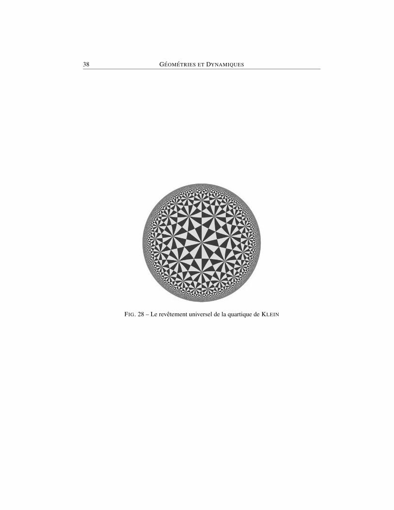
Ces lecons sont tres incompletes. Il y manque en particulier une description du theoremed’uniformisation, l’un des piliers des mathematiques du dix-neuvieme siecle, qui permet dedecrire le revetement universel des surfaces de Riemann. Pour nous faire pardonner, voiciune figure qui illustre de revetement universel de la courbe de KLEIN dont l’equation ho-mogene est x3y + y3z + z3x = 0. Un groupe agit holomorphiquement sur le disque unite,de maniere libre et propre, et la surface de Riemann obtenue par quotient est biholomorphi-quement equivalente a la surface de KLEIN. Pour plus d’informations, on pourra consulterBAVARD : La surface de Klein,www.umpa.ens-lyon.fr/JME/Vol1Num1/artCBavard/artCBavard.pdf.
38 GEOMETRIES ET DYNAMIQUES
FIG. 28 – Le revetement universel de la quartique de KLEIN

E. GHYS, D. SMAI 39
Quiz !
A la fin des six lecons, un questionnaire pour tester vos connaissances ! Repondre par« Vrai » ou « Faux » a chacune des dix assertions suivantes.
[Q1.] La partie de la Terre situee entre l’equateur et le trentieme parallele nord a unesuperficie plus petite que celle de la partie situee au nord du trentieme parallele nord.
Commesin(30)=1/2,lacalottespheriqueaunorddutrentiemeparalleleetlapartiedelaTerresitueeentrel’equateuretletrentiemeparalleleontlamemesuperficieparletheoremed’Archimede!
[Q2.] Sur la carte de Mercator, la zone de latitude superieure a trente degres nord occupela meme surface que la zone situee entre l’equateur et le trentieme parallele nord.
DanslacartedeMercator,unecalottepolairequelconqueestrepresenteeparundemi-plan,d’aireinfinie.L’assertionestdoncfausse.
[Q3.] Sur la carte stereographique a partir du pole sud, la zone situee entre l’equateuret le trentieme parallele nord occupe plus d’espace que la zone situee au nord du trentiemeparallele.
Vraicarlaprojectionstereographiquedilated’autantplusqu’ons’approchedupoledeprojection.
[Q4.] La projection stereographique a partir du pole sud est la meilleure carte conformepour l’hemisphere nord.
Ehbienoui,carladilatationestevidemmentconstantesurlafrontiere,l’equateur,etonpeutdoncappliquerletheoremedeTchebychev.
[Q5.] Pour un pays convexe de l’hemisphere nord la projection stereographique a partirdu pole sud n’est pas la meilleure carte conforme, sauf si ce pays est une calotte polaire.
CelaresulteeneffetdutheoremedeTchebychevcarladilatationdelaprojectionstereographiquenedependquedelalatitudesibienqu’ellen’estconstantesurlafrontierequesicelle-ciestunparallele.

40 GEOMETRIES ET DYNAMIQUES
[Q6.] Il existe un diffeomorphisme conforme de l’ellipsoıde de R3 sur la sphere unite deR3 .
C’estvraimaiscecin’apaseteditdansleslecons!LetheoremedeGaussgarantitl’existencedecartesconformeslocalesmaisl’existencedecartesglobalesresultedel’unicitedelastructuredesurfacedeRiemannsurunesphere,demontreeparRiemann...
[Q7.] Pour tout pays convexe de l’hemisphere sud, il existe une carte qui envoie lesgeodesiques sur des segments de droites.
IlsuffitdeprendrelaprojectionradialeapartirducentredelaTerresurunplanquelconque
[Q8.] On place un obstacle dans un fluide parfait incompressible sans tourbillon. Lavitesse a l’infini est supposee tendre vers le champ de vecteurs uniforme unite horizontal,alors la force de resistance exercee par le fluide sur l’obstacle est perpendiculaire a l’axe desx, meme si la circulation est non nulle (il y a portance mais il n’ y a pas traınee).
Laquestionestmalformulee!S’ils’agitd’unobjetplan,commenousavonsdiscutedanslaleconsurlesfluides,cetenonceestvrai:c’estleparadoxeded’Alembert.S’ils’agitd’unobjetbornededimension3,commeparexempleunconvexe,ilsetrouvequeleparadoxesubsisteetmemesousuneformeforte:iln’yaniportancenitraınee.Onnoteraqu’uneformefermeedanslecomplementaired’unconvexedel’espaceestnecessairementexacte,contrairementacequisepassedansleplan.
[Q9.] Sur une surface de Riemann compacte l’espace vectoriel des formes holomorphesest de dimension finie.
C’estuntheoremedeRiemannquenousavonsrencontre:ladimensionreelledecetespaceest2gougestlegenredelasurface.
[Q10.] L’espace vectoriel des fonctions meromorphes sur une surface de Riemann est dedimension finie.
Faux,carnousavonsvuqu’ilexistedesfonctionsmeromorphesayantunnombrearbitrairementgranddepoles.

E. GHYS, D. SMAI 41
Suggestions de lecturesLa bibliographie sur ce sujet est immense. Ce texte aura ete utile s’il a encourage le lecteur
a en savoir plus et a etudier les preuves. Nous suggerons quelques ouvrages remarquables quipourront servir de portail d’entree au monde des surfaces de RIEMANN.
A. BEARDON, A primer on RIEMANN surfaces. London Mathematical Society Lecture NoteSeries, 78. Cambridge University Press, Cambridge, 1984.
J.B.BOST, Introduction to compact RIEMANN, Jacobian, abelian varieties. From numbertheory to physics (Les Houches, 1989), 64-211, Spinger, Berlin, 1992.
H.COHN, Conformal mappings on RIEMANN surfaces. Reprint of the 1967 edition. DoverBooks on Advanced Mathematics. Dover Publications, Inc., New York, 1980.
R.C. GUNNING, Lectures on RIEMANN surfaces, Jacobi varieties. Mathematical Notes, No.12. Princeton University Press, Princeton, N.J. ; University of Tokyo Press, Tokyo, 1972.
F. KIRWAN, Complex Algebraic Curves, London Mathematical Society Student Texts, 23.Cambridge University Press, Cambridge, 1992.
E. REYSSAT, Quelques aspects des surfaces de RIEMANN. Progress in Mathematics, 77.Birkhauser Boston, Inc., Boston, MA, 1989.
SPRINGER, G, Introduction to RIEMANN surfaces. Addison-Wesley Publishing Company,Inc., Reading, Mass. 1957.
WEYL, H., The concept of a RIEMANN surface. Translated from the third German editionby Gerald R. MacLane. ADIWES International Series in Mathematics Addison-Wesley Pu-blishing Co., Inc., Reading, Mass.-London 1964.
DJAMEL SMAI ETIENNE GHYS
U.S.T.H.B. Unite de MathematiquesFaculte de Mathematiques Pures et Appliquees de l’Ecole
Normale Superieure de Lyon
Laboratoire : A.N.M.E.D.P. U.M.R. 5669 du CNRS
BP 32, El Alia 46, Allee d’Italie16111 Bab-Ezzouar, Alger - Algerie 69364 Lyon Cedex 07- France


Basic geometry of curves andsurfaces
by
RABAH SOUAM
The purpose of these notes is to give a short introduction to the geometry of curves in R2
and surfaces in R3.
1 IntroductionWe will introduce some basic facts about the geometry of curves in R2 and surfaces in R3.Needless to say, this short text will be far from being exhaustive. It is intended for readersnot familiar with differential geometry. We have selected some topics in order to give an ideaabout the subject so that the interested reader can continue by himself this study. In particularwe have chosen to skip the study of curves in R3. We give at the end of these notes somereferences. In all what follows the word smooth will mean of class C∞. All the objects wewill consider (curves, surfaces, mappings...) will be assumed smooth unless otherwise stated.
2 Geometry of curves in R2
2. 1 Local theory of curves in R2
The Euclidean plane R2 will be endowed with its usual orientation, i.e the counter-clockwisesense. e1, e2 will denote the canonical positive orthonormal basis.
Definition 2.1 (parametrized curves) A parametrized curve in R2 is a smooth map α : I →R2 of an open interval I ⊂ R into R2 such that the derivative vector α′(t) does not vanish forevery t ∈ I. For each t ∈ I, there is a well-defined straight line containing α(t) and directedby α′(t). It is called the tangent line to α at t.
Remark 2.1. The reader should be warned that our definition of a parametrized curve coin-cides with the defintion of a regular parametrized curve used in many standard textbooks.
43

44 GEOMETRIES ET DYNAMIQUES
The length of a curve α : I → R2 is the positive (possibly infinite) real number
L(α) =∫I
|α′(t)|dt,
where |α′(t)| is the Euclidean norm of α′(t). It follows from the change of variable formulathat the length is invariant under reparametrizations, i.e if φ : I → J is a diffeomorphism,then L(α φ) = L(α).Given t0 ∈ I, the arc length function of a parametrized curve α : I → R2, measured fromt0, is the function defined by
s(t) =∫ t
t0
|α′(t)|dt.
Since α′(t) 6= 0, the arc length s is a smooth function of t and ds/dt = |α′(t)|. Given thecurve α parametrized by s ∈ (a, b), we may consider the curve β defined on (−b,−a), byβ(−s) = α(s), which has the same trace (i.e same image) as the first one but is traversed inthe opposite direction. We say that these two curves differ by a change of orientation.The arc length function s has a differentiable inverse since ds/dt = |α′(t)| 6= 0. We denoteby abuse of notation its inverse function by t = t(s), which is then defined on the intervals(I) = J. Setting β = α t : J → R2, we obtain a curve which is parametrized by arclength, since |β′(s)| = |α′(t).(dt/ds)| = 1, and which has the same trace as α. We refer toβ as a reparametrization of α by arc length.Given a parametrized curve α : I → R2, for each t ∈ I, we denote by T (t) the unique unitvector tangent to the curve and compatible with its orientation. There is a unique unit vectorN normal to T such that the basis T,N has the same orientation as the standard orientationof R2. N is called the unit normal vector of α. So N defines a differentiable map from I tothe unit circle S1 centered at the origin in R2.Suppose α is parametrized by arc length. Then differentiating the equation |T (s)|2 = 1, wesee that the vector dT/ds(s) is orthogonal to T (s), and so is parallel to N(s). We then setthe definiton:
Definition 2.2 (curvature) The curvature k of the curve α parameterized by arc length s isdefined by
dT
ds(s) = k(s)N(s),
or equivalently by
k(s) = 〈dTds
(s), N(s)〉.
For a better understanding of the curvature, we now see how to compute it in differentsituations.
For a general curve α, not necessarily parametrized by arc length, we have
dT
ds(s) =
dt
ds(t)dT
dt(t) =
1|α′(t)|
dT
dt(t)
and so setting: v(t) = |α′(t)|, we get
k(t) =1v(t)〈dTdt
(t), N(t)〉.

R. SOUAM 45
Note that the sign of k changes when we change either the orientation of α or the orien-tation of R2.
Let (x, y) denote the canonical coordinates in R2. Let then α(t) = (x(t), y(t)) be aparametrized curve in these coordinates. Then
v(t) = (x′2 + y′2)1/2, T (t) =(x′, y′)
(x′2 + y′2)1/2and N(t) =
(−y′, x′)(x′2 + y′2)1/2
and so
k(t) =x′y′′ − x′′y′
(x′2 + y′2)3/2.
Suppose α is parameterized by arc length. Denote by θ(s) the oriented angle betweenthe positive x direction and T (s). This is a locally well defined function (up to an additiveconstant multiple of 2π). We have
T (s) = cos θ(s)e1 + sin θ(s)e2 and N(s) = − sin θ(s)e1 + cos θ(s)e2.
We deduce the following formula which may also be taken as a definition of the curvature:
k(s) =dθ
ds(s).
This formula shows the curvature at s measures the rate of change of the angle which theneighboring tangents make with the tangent at s and so:
The curvature at s measures how rapidly the curve pulls away from the tangent lineat s, in the neighborhood of s.
Consider now a curve α which is given as a graph α(x) = (x, φ(x)) of a differentiablefunction φ. Note that the orientation of the curve is in the direction of increasing x. Then,with the previous notations:
tan θ(x) = φ′(x) andds
dx= (1 + φ′2(x))1/2.
Thus
k(x) =dθ
ds=dθ
dx· dxds
=φ′′(x)
(1 + φ′2(x))3/2.
Given a parametrized curve α : I → R2, and t0 ∈ I, there exists an interval I0 ⊂ Icontaining t0 such that the image α(I0) may be represented as a graph over its tangent lineat t0. Choosing a coordinate system (x, y) so that α(t0) coincides with the origin, T (t0)coincides with e1 and N(t0) coincides with e2, we may assume α(I0) is a graph (x, φ(x)) ofa function φ satisfying φ(0) = φ′(0) = 0. Then, the previous formula shows the curvature att0 is given by the second derivative φ′′(0). In particular if k(t0) 6= 0, the image of the curveα is situated on one side of its tangent line at t0 in a neighborhood of t0. If k(t0) > 0 it issituated in the half-plane into which N(t0) points and in the other half-plane if k(t0) < 0. Ifk(t0) = 0 then, in a neighborhood of t0, the curve may stay on one side of its tangent line att0 or may traverse it.

46 GEOMETRIES ET DYNAMIQUES
Examples. (1) A line segment has curvature zero.
(2) A circle of radius R (centered at the origin) and oriented in the counter-clockwisesense has as an arc length parameterization: α(s) = R(cos(s/R), sin(s/R)), wheres ∈ [0, 2π] and so its curvature is constant and equal to 1/R.
Conversely, suppose α : I → R is a parametrized curve having constant curvature k0.Then differentiating the equation 〈N(s), α′(s)〉 = 0, we get
〈N ′(s), α′(s)〉 = −〈N(s), α′′(s)〉 = −k0.
Since 〈N ′(s), N(s)〉 = 0, we conclude that
N ′(s) = −k0α′(s).
Integrating, we see that N(s) + k0α(s) is a constant vector, say v. If k0 = 0, the normalN(s) = v would be constant and so also α′(s) and integrating again we see that α(I) lies ona line. If k0 6= 0, then
α(s)− v
k0=N(s)k0
and thus ∣∣∣∣α(s)− v
k0
∣∣∣∣ =1|k0|
,
which means α(I) lies on the circle of radius 1/|k0| and center v/k0.More generally, the arc length and the curvature function entirely determine the curve up
to isometries of R2 :
Proposition 2.3 Given a smooth function k : s ∈ I → k(s) ∈ R, the arc lengthparametrized curves α : I → R2 having k as curvature function are given by:
α(s) = (∫
cos θ(s)ds,∫
sin θ(s)ds) + (a, b),
whereθ(s) =
∫k(s)ds+ ϕ,
with ϕ ∈ R and (a, b) ∈ R2.
Proof. Consider a curve α : I → R2 parametrized by arclength whose curvature functionis the given function k. Then the angle θ(s) that α′(s) makes with the positive x axis sat-isfies k(s) = θ′(s). So θ(s) =
∫k(s)ds + ϕ, for some constant ϕ ∈ R. From α′(s) =
(cos θ(s), sin θ(s)), we get
α(s) = (∫
cos θ(s)ds,∫
sin θ(s)ds) + (a, b), (a, b) ∈ R2.
Conversely, it is easy to check that a map α : I → R2 given by the previous formula definesa curve parametrized by arclength with curvature function k.

R. SOUAM 47
Definition 2.4 (the osculating circle) Let α : I → R2 be a parameterized curve and t0 ∈ Isuch that k(t0) 6= 0. The osculating circle of the curve at t0 is the circle of radius 1/|k(t0)|and center α(t0) + 1/k(t0)N(t0). It is the circle which approximates the best the curve at t0(cf. exercise (3) below).
Exercises. (1) Let A be an isometry of R2 and α : I → R2 a parametrized curve. Checkthat the curvature kAα of A α satisfies: kAα(t) = kα(t) if A is orientation preserv-ing and kAα(t) = −kα(t) if A is orientation reversing.
(2) Let α be a parameterized curve and λ > 0 a positive number. Check that the curvaturekα of α and the curvature kλα of the homothetic curve λα, are related by the formula:kλα = 1
λkα.
(3) Let α : I → R2 be a curve parametrized by arc length and s0 ∈ I, such that k(s0) 6= 0.Changing orientation of the curve if necessary, we may assume k(s0) > 0. Let λ ∈ R∗and denoted by Cλ the circle tangent to the curve at s0 with center the point α(s0) +λN(s0). Check that if λ > 1/k(s0) (respectively if λ < 1/k(s0)) then there is a smallneighborhood J of s0 in I such that α(J) is contained inside (respectively outside) thecircle Cλ. Hint: study, near s0, the function f(s) = |α(s)− (α(s0) + λN(s0))|2.Check that, in general, the curve traverses its osculating circle.
2. 2 Global theory of curves in R2
Definition 2.5 By a closed parametrized curve in R2 we mean a parametrized curve α :[a, b] → R2 which is smooth up to the endpoints a and b such that α and all its derivativesagree at a and b :
α(a) = α(b), and α(k)(a) = α(k)(b), for all k ≥ 1.
Equivalently a closed curve may be defined as a smooth map: α : S1 → R2, defined ona circle S1 with non vanishing derivative. It is said simple, or embedded, if it has no self-intersections, that is if α is an injective map.
We may sometimes identify a simple closed curve with its image.
Variation of the length
We will derive the formula for the variation of the length of a closed curve. This will give usanother interpretation of the curvature.
Let α : s ∈ [0, l]→ α(s) ∈ R2 be a closed curve. By a variation of α we mean a smoothmap:
F : [0, l]× (−ε, ε)→ R2,
such that, for each t, the map F (., t) defines a closed curve and α = F (., 0). Denote byL(t) the length of F (., t). We may assume that α is parametrized by arc length. Then, sinceF (0, t) is parametrized by arc length, we have:
dL
dt(0) =
d
dt|t=0
∫ l
0
〈∂F∂s
,∂F
∂s〉 12 ds =
12
∫ l
0
〈 ∂2F
∂t∂s,∂F
∂s〉|t=0ds,

48 GEOMETRIES ET DYNAMIQUES
Integrating by parts, we obtain
dL
dt(0) = −1
2
∫ l
0
〈∂F∂t,∂2F
∂s2〉|t=0ds = −1
2
∫ l
0
〈∂F∂t|t=0, k(s)N(s)〉ds.
The mapping ∂F∂t |t=0 ∈ C∞([0, l],R2) is a vector field along α and is called the variation
vector field associated to the variation F. We may consider the space C of closed curves inR2. The tangent space TαC at a curve α : [0, l] → R2 may be identified with C∞([0, l],R2)and endowed with the inner product:
〈V1, V2〉 =∫ l
0
〈V1(s), V2(s)〉ds, V1, V2 ∈ C∞([0, l],R2),
where we assumed the curve is parametrized by arclength. Thus the vector field − 12kN
along α may be viewed as the gradient at α of the length functional defined on the space C.
The Jordan curve theorem
The Jordan curve theorem asserts that a simple closed curve divides the plane into two con-nected components, an unbounded one, called its exterior, and a bounded one called its inte-rior, which moreover is homeomorphic to a disk. We shall refer to the latter as the domainbounded by the curve. Although intuitive, this fact, which is also true for C0 maps, is not soeasy to prove. For a proof see [2].Remark 2.2. Let α : t ∈ [a, b] → (x(t), y(t)) ∈ R2 be a simple closed curve and let Ωdenote its interior domain. The curve is said to be positively oriented if its oriented unitnormal points towards Ω.
We now derive formulae for the areaA of the domain Ω bounded by a simple closed curveα. Using Stokes theorem, the area A can be written as follows:
A =∫
Ω
dx ∧ dy =∫
Ω
d(xdy) = −∫
Ω
d(ydx) =∫ b
a
x(t)y′(t)dt = −∫ b
a
x′(t)y(t)dt.
Another useful formula for the area is as follows. Denote by X the position vector fieldon R2, i.e X(x, y) = (x, y). The divergence of X is divX = 2. So if α : [0, l] → R2 ispositively oriented and parametrized by arc length, using the divergence theorem we get:
A =12
∫Ω
(divX) dx ∧ dy = −12
∫ l
0
〈α(s), N(s)〉ds.
The isoperimetric inequality
The isoperimetric problem is stated as follows: among all domains having the same boundarylength, find those of maximum area. The solutions to this problem in the plane are the circulardisks. The problem can be formulated in all dimensions and the result extends: the solutionsare the round balls. There are many different proofs of this fact. We present one which ismaybe the cheapest one but has the inconvenient that, so far, it has not been generalized tohigher dimensions. The isoperimetry property of the circular disks is a consequence of thefollowing isoperimetric inequality:

R. SOUAM 49
Theorem 2.6 Let C be a simple closed curve in R2 with length L, and let A be the area ofthe domain bounded by C. Then
L2 ≥ 4πA,
and equality holds if and only if C is a circle.
For the proof, we need the following:
Lemma 2.7 (Wirtinger’s inequality) Let f ∈ C1(R) a 2π-periodic function with zero mean,that is
∫ 2π
0f(t)dt = 0. Then ∫ 2π
0
f ′2(t)dt ≥∫ 2π
0
f2(t)dt,
with equality if and only if f(t) = a cos(t) + b sin(t).
Proof. f and f ′ are equal to their Fourier series in the L2[0, 2π] sense. Since∫ 2π
0f(t)dt = 0,
the Fourier series expansion of f reads:
∞∑n=1
an cos(nt) + bn sin(nt)
and that of f ′ reads∞∑n=1
nbn cos(nt)− nan sin(nt)
By Parseval’s identity we have:
1π
∫ 2π
0
f2(t)dt =∞∑n=1
a2n + b2n
1π
∫ 2π
0
f ′2(t)dt =∞∑n=1
n2a2n + n2b2n.
The result follows immediately.
Proof of the isoperimetric inequality. Note that if we perform a homothety of magnitude λ,then the length is multiplied by λ and the area is multiplied by λ2. So, up to a homothety,we may assume the curve has length 2π. We may also assume it is positively oriented andparametrized by arc length, α = (x, y) : [0, 2π] → R2. Up to a translation in R2, we mayassume the center of gravity of the curve is at the origin, i.e∫ 2π
0
xdt =∫ 2π
0
ydt = 0.
Since the curve is parametrized by arclength we have∫ 2π
0
(x′2 + y′2)dt = 2π = L,

50 GEOMETRIES ET DYNAMIQUES
whereas
A =∫ 2π
0
xy′dt.
So
2(π −A) =∫ 2π
0
(x′2 + y′2 − 2xy′)dt =∫ 2π
0
(x′2 − x2)dt+∫ 2π
0
(x− y′)2dt.
The integral in the last term is nonnegative by Wirtinger’s inequality, so A ≤ π. If equalityholds then x(t) = a cos t + b sin t and y(t) = a sin t − b cos t, and the curve is a circleparametrized by arc length.
Remark 2.3. It follows that the isoperimetric inequality is in fact true for any bounded regulardomain in R2. A domain is said to be regular if each of its boundary components is the trace(i.e the image) of either a one-to-one parametrized curve defined on R or a simple closedcurve. A compact regular domain is then bounded by a finite number of simple closed curvesand is contained in the interior Ω of one of them, this follows easily from the Jordan curvetheorem. The isoperimetric inequality (and the characterization of the equality case) followsdirectly from the result for Ω by ”filling the holes”.
The rotation index and total curvature of simple closed curves
The rotation index of a closed curve (not necessarily simple) is the algebraic number of timesthe tangent vector rotates along the curve. We need some preparatory material before statingsome results about the rotation index. We refer to [1] for the proofs. In order to give arigourous definition of the rotation index we need to introduce the notion of degree of mapsS1 → S1. Denote by p : R → S1 = R/2πZ the canonical projection. We then have thefollowing:
Lemma 2.8 (Paths lifting property) Let f ∈ C0([a, b], S1), and x ∈ p−1(f(a)). Then thereexists a unique map f ∈ C0([a, b],R) such that f = p f and f(a) = x.The map f is called a lift of f. Any two lifts differ by an integer mutiple of 2π.
Proof. we leave the proof as an exercise. Hint: consider the set I = t ∈ [a, b], f : [0, t] →R has a (continuous) lift f : [0, t]→ R, f(a) = x and show that it is non empty, openand closed. See [1] for the details.
Definition 2.9 (the degree of maps S1 → S1) Let f : S1 → S1 be a continuous map. Applythe above lemma to obtain a map f : [0, 2π]→ R lifting f p. The degree of f is the integer
deg(f) :=f(2π)− f(0)
2π.
Remark 2.4. (1) The degree is indeed an integer since f(2π) = f(0), and does not dependon the lift since any two lifts differ by an additive constant. One can also replace 0 byany s ∈ R, and gets the same result setting
deg(f) =f(2π + s)− f(s)
2π.

R. SOUAM 51
(2) If one takes a periodic map having a period L not necessarily equal to 2π, that is a mapf : R/LZ→ R/2πZ, the degree is then given by:
deg(f) =f(L+ s)− f(s)
2π.
A map f1 ∈ C0(S1, S1) is said to be homotopic to a map f2 ∈ C0(S1, S1) if there is acontinuous map:
H : [0, 1]× S1 → S1,
such thatH(0, t) = f1(t),
H(1, t) = f2(t).
This defines an equivalence relation between maps in C0(S1, S1). A fundamental propertyof the degree is its invariance under homotopy:
Homotopic maps have the same degree.See [1] for the details and further reading.
Definition 2.10 (The rotation index of closed curves) Let α : S1 → R2 be a closed planecurve and T (t) = 1
|α′(t)|α′(t), its tangent unit vector at t ∈ S1. T may be seen as a map
T : S1 → S1, called the tangent map. The rotation index of the curve α is by definition thedegree of its tangent map T.
Note that the rotation index depends on the orientation (and is independent on the choiceof orientation preserving parametrizations). An important fact about the rotation index is thefollowing:
Theorem 2.11 (The turning tangent theorem) The rotation index of a simple closed curveis ±1, where the sign depends on the orientation of the curve.
Proof. We outline the proof and refer to [1], [2] or [5] for the details and figures. The ideaof the proof is to construct a homotopy between the tangent map and a secant map which hasdegree one. Let α : [0, l] → R2 be a simple closed curve. We may easily find a line L inthe plane which is tangent to α([0, l]) at some point p and such that the whole trace α([0, l])is located on one side of L (take a line not touching the curve and move it parallel to itselfuntil it touches the curve for the first time). We may assume without loss of generality thatp = α(0). Consider now the triangle
∆ = (t1, t2) ∈ [0, l]× [0, l]; 0 ≤ t1 ≤ t2 ≤ l
and define a ”secant map” Ψ : ∆→ S1 by
Ψ(t1, t2) =α(t2)− α(t1)|α(t2)− α(t1)|
for t1 6= t2, (t1, t2) ∈ ∆− (0, l)
Ψ(t, t) =α′(t)|α′(t)|
, Ψ(0, l) = − α′(0)|α′(0)|
.

52 GEOMETRIES ET DYNAMIQUES
Ψ is well defined because the curve is simple. It is easily seen to be continuous. Let A =(0, 0), B = (0, l), C = (l, l) be the vertices of the triangle ∆. Note that Ψ restricted to theside AC is the tangent map of α. The tangent map is thus homotopic to the restriction of Ψto the remaining sides AB and BC. It is thus enough to see the latter map has degree ±1.
Assume the orientations of the plane and the curve are such that the oriented angle fromα′(0) to −α′(0) is π. The restriction of Ψ to AB covers half of S1 in the positive direction,and the restriction of Ψ to BC covers the remaining half also in the positive direction. Thus,the degree of Ψ restricted to AB and BC is +1. If we reverse the rientation, we obtain −1for this degree. This completes the proof.
Definition 2.12 (Total curvature of closed curves) Let α : [0, l] → R2 be a closed curveparametrized by arc length. The total curvature of α is by definition the quantity:∫ l
0
k(s)ds.
Note that the total curvature depends on the orientation of the curve. Let α : [0, l] → R2
be a simple closed curve parametrized by arc length. A lift T : [0, l]→ R, of the tangent mapT : [0, l] → S1 is a measure of the oriented angle between the positive x axis and T (s). Wehave seen that k(s) = dT (s)/ds. So:∫ l
0
k(s)ds = T (l)− T (0) = 2πdeg(T ).
It follows that:
The total curvature of a closed curve is equal to 2π times its rotation index.
A consequence of the Theorem 2.11 is thus:
Corollary 2.13 The total curvature of a simple closed curve is equal to ±2π.
Remark 2.5. The total curvature is equal to 2π in case the curve is positively oriented.
Convexity
We now give a converse to Corollary 2.13.
Proposition 2.14 Let α : [0, l]→ R2 be a closed curve with∫ l
0k(s)ds = ±2π. Assume its
curvature does not change sign. Then α is simple. Moreover, for each s ∈ [0, l], the traceα([0, l]) lies in one of the closed half-planes determined by the tangent line at s.
Proof. Up to a change of orientation on the curve, we may assume k ≥ 0. Take any liftT : [0, l] → R of the tangent map T : [0, l] → S1. Since k does not change sign, T ismonotone. Let s0 ∈ [0, l], we will show the trace of α lies in one of the closed half-planesdetermined by the tangent line ∆ at s0.Assume this is not the case, there exist then two pointsp, q on the curve lying on different sides of ∆. Let N(s0) be the unit normal vector at s0, andconsider the function:
h(s) = 〈α(s)− α(s0), N(s0)〉, s ∈ [0, l].

R. SOUAM 53
Then h takes positive and negative values (its values at p and q are of opposite sign by hy-pothesis). By compactness it then has a positive maximum at a point s1 6= s0 and a negativeminimum at a point s2 6= s0. Thus two of the unit tangent vectors at s0, s1, s2 coincide,say for instance at s0 and s1. Then T (s0) − T (s1) ∈ 2πZ. Since the rotation index is one,|T (s0)−T (s1)| < 2π, so necessarily T (s0) = T (s1) and then by monotonicity, T is constanton the interval [s0, s1] (assuming s0 < s1). Therefore k vanishes identically on [s0, s1] andso α([s0, s1]) ⊂ ∆, which is a contradiction.
Let us show now α is simple. Assume there are 0 ≤ s0 < s1 < l, such that α(s0) =α(s1). If the tangent lines at s0 and s1 do not coincide, this clearly contradicts the aboveproperty about the position of the curve with respect to its tangent lines. Therefore eitherα′(s0) = α′(s1) or α′(s0) = −α′(s1). In the first case, as before, the monotonicity of Tand the fact that the rotation index is one imply that α([s0, s1]) is contained in a line. Sinceα′(s0) = α′(s1), this implies the existence of a zero of α′, which is a contradiction. Sonecessarily α′(s0) = −α′(s1). Consider then, as before, the function
h(s) = 〈α(s)− α(s0), N(s0)〉, s ∈ [s0, s1].
Then h(s0) = h(s1) and so h reaches its maximum on [s0, s1] at some point s2 , s0 < s2 <s1. Then α′(s2) coincides either with α′(s0) or α′(s1) and we are led to a contradiction asbefore. This completes the proof.
Exercise. Give examples showing the necessity of each of the hypotheses in the Proposition2.14.
Definition 2.15 A curve satisfying the hypotheses of the Proposition 2.14 is called convex.
Remark 2.6. Consider a simple closed curve and denote by Ω the domain it bounds. It canbe shown that convexity of the curve is equivalent to the convexity of Ω in the ordinary sense,i.e for each points p, q inside Ω, the segment joining them is entirely inside Ω. For a proofsee [1].
3 Basic geometry of surfaces in R3
We assume in this section some familiarity with the notion of differentiable surfaces. Allsurfaces will be assumed connected unless otherwise stated.
3. 1 Local theory of surfaces in R3
We first recall briefly some basic notions about surfaces in R3 and refer to the literature ([2],[5]) for further details.
Definition 3.1 (Surfaces in R3) A non empty subset S ⊂ R3 is said to be a surface if foreach p ∈ S there exists an open set U ⊂ R2, an open neighborhood V of p in S and a smoothmap X : U → R3 such that:
• X(U) = V.

54 GEOMETRIES ET DYNAMIQUES
• X : U → V is a homeomorphism.
• (dX)q : R2 → R3 is injective for each q ∈ U.
X is called a parametrization and the (cartesian) coordinates (u, v) on U are called localcoordinates on S. The second (technical) condition ensures that S is a submanifold of R3.Wepoint out that the notions to be introduced in the sequel make sense for immersed surfaces.An immersed surface in R3 is a smooth map X : S → R3 from an abstract surface S into R3
such that (dX)p is injective for each p ∈ S.
Definition 3.2 (Tangent plane) Let S ⊂ R3 be a surface and p ∈ S. A vector w ∈ R3 issaid to be tangent to S at p if there exists a curve α : (−ε, ε)→ S, ε > 0, such that α(0) = pand α′(0) = w. The set of all such vectors is denoted by TpS.
If X : U → S is a parametrization with p ∈ X(U) then it is not difficult to checkthat TpS = (dX)X−1(p)(R2). In particular TpS is a linear subspace of R3 and is called thetangent plane to S at p. The affine subspace p+ TpS of R3 is called the affine tangent planeto S at p.
The first fundamental form
Definition 3.3 (The first fundamental form) Let S be a surface in R3 and p ∈ S. Thetangent space TpS inherits an inner product, denoted by Ip, from the inner product on R3.More precisely,
Ip(w1,w2) = 〈w1,w2〉, for all w1,w2 ∈ TpS.
I is called the first fundamental form of S.
I measures the norm of vectors tangent to S and hence the length of curves on S. Letc : J → S be a parameterized curve on S (J an interval of R) and let c′(t) = dc
dt (t) ∈ Tc(t)Sdenote its tangent vector at t ∈ J, then the length of c is given by
L(c) =∫J
√Ic(t)(c′(t), c′(t))dt.
The length is invariant under reparametrizations.If X : U ⊂ R2 → X(U) is a local parametrization of an open set X(U) ⊂ S, and
w = αXu + βXv a tangent vector then:
I(w,w) = α2〈Xu,Xu〉+ 2αβ〈Xu,Xv〉+ β2〈Xv,Xv〉
Let E(u, v) = 〈Xu, Xv〉, F (u, v) = 〈Xu, Xv〉, and G(u, v) = 〈Xv, Xv〉, denote the coef-ficients of the first fundamental form in the basis Xu, Xv. Usually one represents the firstfundamental form by the arclength element ds written as
ds2 = Edu2 + 2Fdudv +Gdv2,

R. SOUAM 55
which means that if γ : J → X(U), γ(t) = X(u(t), v(t)) is a curve in X(U), then its arclength satisfies:
ds
dt= |γ′(t)| =
√E(dudt
)2 + 2F(dudt
)(dvdt
)+G
(dvdt
)2.
Its length is given by the integral:∫J
√E(dudt
)2 + 2F(dudt
)(dvdt
)+G
(dvdt
)2dt.
Definition 3.4 Let S and S′ be two surfaces in R3. A diffeomorphism φ : S → S′ is said tobe an isometry if for each p ∈ S and all w1,w2 ∈ TpS
Ip(w1,w2) = Iφ(p)(dφp(w1),dφp(w2)).
A map φ : V → S′ of a neighborhood V of p ∈ S is a local isometry at p if there exists aneighborhood V ′ of φ(p) in S′ such that φ : V → V ′ is an isometry. If there is a local isom-etry into S′ at every p ∈ S, the surface S is said to be locally isometric to S′. The surfaces Sand S′ are locally isometric if S is locally isometric to S′ and S′ is locally isometric to S.
Exercise. Suppose there are local parametrizations X : U → X(U) of S and X ′ : U →X ′(U) of S′ such that E = E′, F = F ′ and G = G′. Check that the map: φ : X ′ X−1 :X(U)→ X ′(U) is an isometry.
Examples. (1) A graph (x, y, h(x, y)) of some function h : U → R3, U ⊂ R2 has as aparametrization the map:
(x, y) ∈ U → X(x, y) = (x, y, h(x, y)).
The coefficients of the first fundamental form are:
E(x, y) = 〈Xx, Xx〉 = 1 + h2x,
F (x, y) = 〈Xx, Xy〉 = hxhy,
G(x, y) = 〈Xy, Xy〉 = 1 + h2y.
So,ds2 = (1 + h2
x)dx2 + 2hxhydxdy + (1 + h2y)dy2.
For instance, the plane z = 0 has as arclength element: ds2 = dx2 + dy2.
(2) Let α : s ∈ (a, b) → ((x(s), y(s)) ∈ R2 be a curve in R2 parametrized by arc length.The right cylinder with base the curve α in R3 has the following parametrization:
X(s, t) = (x(s), y(s), t), s ∈ (a, b), t ∈ R.
ThenXs = (x′(s), y′(s), 0), Xt = (0, 0, 1),

56 GEOMETRIES ET DYNAMIQUES
soE = 1, F = 0, G = 1.
We have thus found (local) coordinates on the cylinder where the first fundamentalform is the same as the first fundamental form of a plane. Thus the plane and a cylinderare locally isometric.
(3) Consider a curve t ∈ (a, b)→ (x(t), z(t)) in the (x, z)-plane in R3 and assume x(t) >0. Rotating this curve around the z-axis, one obtains a surface of revolution whichadmits the parametrization:
X(θ, t) = (x(t) cos θ, x(t) sin θ, z(t)), a < t < b, 0 ≤ θ ≤ 2π.
The coefficients of the second fundamental form in these coordinates are then:
E = (x(t))2, F = 0, G = (x′(t))2 + (z′(t))2.
The arclength element is:
ds2 = (x(t))2dθ2 + ((x′(t))2 + (z′(t))2)dt2.
3. 2 The Gauss mapIn order to study the way a surface curves into space one is laid, as in the case of curves inthe plane, to study the variation of the tangent plane or equivalently the variation of the unitnormal to the tangent plane. This leads to the notion of Gauss map which is fundamental inthe theory of surfaces in R3. We point out again that the following study is local and thus isvalid for immersed surfaces.
Definition 3.5 Let S ⊂ R3 be an orientable surface in R3, oriented by the choice of a(differentiable) unit normal N. The map N : S → R3 takes its values in the unit sphereS2 = (x, y, z) ∈ R3, x2 + y2 + z2 = 1. It can thus be viewed as a map
N : S → S2,
and is called the Gauss map of S.
For any q ∈ S2, the tangent plane TqS2 is the linear plane orthogonal in R3 to the vectorq. So for p ∈ S, the tangent space TN(p)S2 coincides with TpS and so the linear map dNp :TpS → TN(p)S2 is a linear endomorphism of TpS,
dpN : TpS → TpS.
Definition 3.6 The linear endomorphism −dNp : TpS → TpS is called the shape operatoror Weingarten map of S at p.
The linear map dNp : TpS → TpS operates as follows. Let p ∈ S and w ∈ TpS. If α(t)is a parametrized curve in S with α(0) = p and α′(0) = w, we consider the parametrizedcurve N α(t) = N(t) in S2 ⊂ R3. Then
dNp(w) =d
dt(N α)(t)|t=0 = N ′(0).
R. SOUAM 57
Examples. (1) For a plane, say the (x, y)-plane, N = (0, 0, 1) at each point and so theshape operator of the plane vanishes identically.
(2) Consider the sphere S2a(r) ⊂ R3 of radius r centered at a point a and oriented by the
interior unit normal N(p) = − 1r (p − a), p ∈ S2
a(r). Then dNp = − 1r Idp, where Idp
is the identity map of TpS2a(r).
(3) An important feature of the shape operator is the following:
Proposition 3.7 dNp : TpS → TpS is symmetric.
Proof. Take any local parametrization X : (u, v) ∈ U → S around p ∈ S. Since for eachq ∈ U , Xu(q), Xv(q) is a basis of TX(q)S, it is enough to check that:
〈dN(Xu), Xv〉 = 〈Xu, dN(Xv)〉.
Since 〈N X,Xv〉 = 0, differentiating with respect to u, we get
〈dN(Xu), Xv〉 = 〈(N X)u, Xv〉 = −〈(N X)uv, X〉,
and symmetrically,
〈dNp(Xv), Xu〉 = 〈(N X)v, Xu〉 = −〈(N X)vu, X〉.
The result now follows from the Schwarz lemma.
Being symmetric, the operator −dNp has two real eigenvalues and can be diagonalizedin an orthonormal basis. We thus set the following
Definition 3.8 The eigenvalues κ1 and κ2 of the symmetric linear map−dNp : TpS → TpSare called the principal curvatures of S at p, and its eigenvectors are called the principaldirections of S at p. A curve on S whose tangent vector is a principal direction at each pointis called a line of curvature.
The half of the trace of −dNp,
H(p) = −12
tr dNp =κ1 + κ2
2,
is called the mean curvature of S at p.The determinant of −dNp,
K(p) = det dNp = κ1κ2,
is called the Gaussian curvature of S at p.

58 GEOMETRIES ET DYNAMIQUES
The second fundamental form
Definition 3.9 (The second fundamental form) The symmetric bilinear form on TpS atp ∈ S defined by
IIp(w1,w2) = −〈dNp(w1),w2〉 = −〈w1,dNp(w2)〉
is called the second fundamental form of S at p.
Remark 3.1. If we change the orientation of the surface (i.e replace N by −N ), thenII, κ1, κ2 and H change by sign but K does not change.
Examples. (1) For a plane, at each point II = 0, κ1 = κ2 = H = K = 0.
(2) The sphere S2a(r) ⊂ R3 of radius r centered at a point a and oriented by the interior unit
normal has as second fundamental form II = 1r I, and as curvatures κ1 = κ2 = H = 1
rand K = 1
r2 everywhere.
Note that in these two examples, at each point, all the tangent directions are principal,otherwise said the second fundamental form is a multiple of the first one. A point on asurface where the second fundamental form is a multiple of the first one is called an umbilicpoint. A surface is called totally umbilic if all its points are umbilic. So planes and spheresare totally umbilic. Conversely, it can be shown that a totally umbilic surface is a part of aplane or a sphere (cf. [2]).
Curvature of normal sections
The second fundamental form has the following interesting interpretation: let p ∈ S andw ∈ TpS a unit tangent vector and consider the affine plane Πw through p spanned by w andN(p). Near p, the intersection Πw ∩ S is a curve in the plane Πw which is the graph of asmooth function over the axis determined by w. Orient the plane Πw by the basis w,N(p).Let α be a parametrization by arc length of the intersection curve with α(0) = p and α′(0) =w. Differentiating the equality 〈N(α(s)), α′(s)〉 = 0, we get
−〈dNp(α′(0)), α′(0)〉 = 〈N(α(0)), α′′(0)〉
that is
IIp(w,w) = 〈N(p), α′′(0)〉.
So: The second fundamental form calculated on the unit vector w coincides with the curva-ture at p of the normal section defined by w.
Also, it is easily seen that on a two dimensional Euclidean space, the eigenvalues of asymmetric operator are the extremums (the maximum and the minimum) on the unit sphereof the associated quadratic form. It follows that the principal curvatures at p ∈ S are theextremums of the curvatures of plane sections at p defined by the normal N(p).
R. SOUAM 59
The Gauss map in local coordinates
In this section, we consider a local parametrization X : U → S. We can choose the unitnormal field N determined by the relation
(N X)(u, v) =Xu ∧Xv
|Xu ∧Xv|.
Let (aij) be the matrix of dN in the basis Xu, Xv. This means:
dN(Xu) = (N X)u = a11Xu + a21Xv,
dN(Xv) = (N X)v = a12Xu + a22Xv.
Denote by M the matrix associated to the first fundamental form in the coordintaes (u, v) :
M =(E FF G
)Set
e = −〈(N X)u, Xu〉 = 〈N X,Xuu〉
f = −〈(N X)v, Xu〉 = 〈N X,Xuv〉 = 〈N X,Xvu〉 = −〈(N X)u, Xv〉
g = −〈Nv, Xv〉 = 〈N X,Xvv〉.
These are called the coefficients of the second fundamental form in the coordinates (u, v).Denote by Σ the associated matrix:
Σ =(e ff g
)Then, it is easily checked that Σ = −M(aij) and so:
(aij) = −M−1Σ.
The mean and Gaussian curvatures are therefore given by:
2H = −tr(aij) = tr(M−1Σ) =eG− 2fF + gE
EG− F2,
K = det(aij) =det Σdet M
=eg − f2
EG− F2.
Example (Graphs). For a surface given as a graph S = (x, y, h(x, y), h : U ⊂ R2 → R,
Xx = (1, 0, hx), Xy = (0, 1, hy),
Xxx = (0, 0, hxx), Xxy = (0, 0, hxy), Xyy = (0, 0, hyy),
(N X)(x, y) =(−hx,−hy, 1)
(1 + h2x + h2
y)1/2,

60 GEOMETRIES ET DYNAMIQUES
e = 〈N X,Xxx〉 =hxx
(1 + h2x + h2
y)1/2, g = 〈N X,Xyy〉 =
hyy(1 + h2
x + h2y)1/2
f = 〈N X,Xxy〉 =hxy
(1 + h2x + h2
y)1/2.
So
K =hxxhyy − h2
xy
(1 + h2x + h2
y)2,
2H =(1 + h2
x)hyy − 2hxhyhxy + (1 + h2y)hxx
(1 + h2x + h2
y)3/2.
Once known the values of H and K, the principal curvatures are then the roots of the poly-nomial X2 − 2HX +K, that is, κi = H ±
√H2 −K, i = 1, 2.
Given a point p ∈ S, up to a translation and a rotation in space, we may assume the pointp coincides with the origin and the tangent plane TpS coincides with the plane z = 0. Wemay then represent S near p as a graph of a function h with h(0, 0) = 0 and hx(0, 0) =hy(0, 0) = 0, then the second fundamental form at p calculated on a tangent vector (x, y) isgiven by:
IIp((x, y), (x, y)) = hxx(0, 0)x2 + 2hxy(0, 0)xy + hyy(0, 0)y2
and so it coincides with the hessian d2h(0, 0) of h at (0, 0).In particular, if K(p) = det d2h(0, 0) = hxx(0, 0)hyy(0, 0)−h2
xy(0, 0) is > 0 then h haseither a local maximum or minimum at (0, 0) and so S lies on one side of its affine tangentplane in some neighborhood of p, the same side as N(p) if κ1, κ2 > 0, the opposite side ifκ1, κ2 < 0. In this case, the point p is called elliptic.
If K(p) < 0, that is, if κ1, κ2 have opposite signs, then h changes sign in any neighbor-hood of (0, 0) ans so S traverses its affine tangent plane in any neighborhood of p. The pointp is called a saddle point or a hyperbolic point.
If K(p) = 0 but IIp 6= 0, which means one of the principal curvatures is 0 and the otheris non zero, then p is called a parabolic point. If IIp = 0, that is to say k1 = k2 = 0, then pis called a flat point.
Example (Surfaces of revolution). Let t ∈ (a, b)→ (x(t), z(t)) be a curve in the (x, z)-planein R3 with x(t) > 0. Rotating this curve around the z-axis, one obtains a surface of revolutionwhich admits the parametrization:
X(θ, t) = (x(t) cos θ, x(t) sin θ, z(t)), a < t < b, 0 ≤ θ ≤ 2π.
We will now see that the meridians t → X(θ, t) and the parallels θ → X(θ, t) are lines ofcurvature. Since the surface is invariant under rotation around the z-axis, it is enough to checkthat the curve t→ (x(t), 0, z(t)) is a line of curvature. Indeed, by symmetry this will show allthe meridians are lines of curvature and also all the parallels since the two principal directionsare orthogonal at each point. Now, just notice that by symmetry the unit normal to the curvet → (x(t), 0, z(t)) in the (x, z)-plane is normal to the surface and so its differential will beparallel to the tangent vector (x′(t), 0, z′(t)), which means the curve is a line of curvature.

R. SOUAM 61
Let us compute the principal curvatures. Again, by symmetry, it is enough to do thecomputation on the curve t→ (x(t), 0, z(t)). This curve is a normal section, so the associatedprincipal curvature is equal to its curvature as a plane curve provided the plane is correctlyoriented .
Therefore (cf. 2. 1):
κ1 =x′z′′ − x′′z′
(x′2 + z′2)3/2.
As a unit normal to the curve, we may take:
N(0, t) =(−z′, 0, x′)
(x′2 + z′2)1/2.
So the unit normal to the surface at the point X(θ, t) is obtained by rotating N(0, t) aroundthe z-axis by the angle θ :
N(θ, t) =(−z′ cos θ,−z′ sin θ, x′)
(x′2 + z′2)1/2.
For t fixed, put α(θ) = X(θ, t), then:
II(α′(θ), α′(θ)) = −〈Nθ, α′(θ)〉 =xz′
(x′2 + z′2)1/2.
Hence:
κ2 =II(α′(θ), α′(θ))|α′(θ)|2
=z′
x(x′2 + z′2)1/2.
3. 3 The area element and the area formLet S be a surface in R3 and X : U −→ R3 a local parametrization, U ⊂ R2, and asusual denote by E,F,G the coefficients of the first fundamental form in these coordinates.We consider the measure on U given by
√EG− F 2dudv. If f : S −→ R is a continuous
function with compact support in X(U), its integral is by definition:∫S
f =∫U
(f X)(u, v)√EG− F 2dudv.
The value of the integral does not depend on the choice of paramaterization. Indeed if X ′ :U ′ → S is another parametrization with X(U) ∩ X ′(U ′) 6= ∅, set φ = X ′
−1 X, V =X−1(X(U) ∩ X ′(U ′)) and V ′ = X ′
−1(X(U) ∩ X ′(U ′)). If f is a function with compactsupport in X(U) ∩X ′(U ′), then by the change of variables formula:∫V ′
(fX ′)(u′, v′)√E′G′ − F ′2du′dv′ =
∫V
(fX ′)(φ(u, v))√E′G′ − F ′2 |det dφ|dudv
If we denote by M (resp. M ′) the matrix of the first fundamental form in the coordinates(u, v) (resp. in the coordinates (u′, v′)) and by P the change of coordinates matrix from the
62 GEOMETRIES ET DYNAMIQUES
basis Xu, Xv of R2 to the basis X ′u′ , X ′v′, then M = PM ′tP. The conclusion followssince P is also the matrix of dφ in the bases ∂∂u ,
∂∂v and ∂
∂u′ ,∂∂v′
Using a partition of unity, one then extends this defintion to functions with compact sup-port in S and it can be checked this definition is independent on the choice of the partitionof unity. In this way we have defined a measure on S called the area element or canonicalmeasure and usually denoted by dA. In particular the area of a domain Ω in S is by definitionthe integral of the function identically equal to 1:
area(Ω) =∫
Ω
dA.
When S is orientable and oriented by a choice of a unit normalN, one can define a differential2-form ω on S as follows:
ω(p)(w1,w2) = det(w1,w2,N(p)), p ∈ S, w1,w2 ∈ TpS.
ω(p)(w1,w2) is the algebraic area in TpS of the quadrelateral determined by the ordered pair(w1,w2). The form ω is called the area form on S. Integrating a function f on S with respectto the area element amounts to the same to integrating the 2-form fω.
Denote by σ the area form on the unit sphere oriented by its exterior normal. Then, thepull-back by N of σ is such that for w1,w2 ∈ TS :
N∗σ(w1,w2) = σ(dN(w1),dN(w2))= det(dN(w1),dN(w2),N)= det(dN)det(w1,w2,N).
So we get the following relation:N∗σ = Kω.
N preserves the orientation at points where K > 0 and reverses it at points where K < 0. Ifp ∈ S, and U a neighborhood of p which contracts down to p, it then follows that:
K(p) =
limU→p
area(N(U))area(U)
if K(p) ≥ 0
− limU→p
area(N(U))area(U)
if K(p) ≤ 0.
3. 4 Conformal coordinatesA parametrization X : U → X(U) ⊂ S of an open set X(U) in a surface S is called aconformal parametrization if there exists a (necessarily positive) function λ : U → R, suchthat the arc length element on U takes the form:
ds2 = λ(u, v)2(du2 + dv2).
Equivalently, this means that in U :
|Xu|2 = |Xv|2, 〈Xu, Xv〉 = 0.
We have the following non-trivial theorem.

R. SOUAM 63
Theorem 3.10 (Existence of conformal coordinates) Let S be an immersed surface in R3.Then around each point in S there exists a conformal parametrization.
Remark 3.2. This theorem, which is of fundamental importance, is valid on any abstractRiemannian surface. A Riemannian surface is a surface (not necessarily immersed in R3)whose tangent plane at each point is endowed with an inner product which depends smoothlyon the point. This means that when written in any local chart, the coefficients of the innerproduct are smooth functions.
Exercise (Riemann surface structure). Let S be a surface in R3 (more generally any Rieman-nian surface). By the Theorem 3.10 there exists an atlas of conformal charts. The change ofcoordinates maps may be viewed as functions between open sets in C. Prove that each suchfunction is either holomorphic or anti-holomorphic. In particular, if S is orientable, we canget an atlas of conformal charts and the change of coordinates maps are holomorphic. Thesurface S admits thus an underlying complex structure compatible with its metric. A complexmanifold with complex dimension 1 is by definition a Riemann surface.
In a conformal parametrization, the mean curvature has a particularily simple expression:
Proposition 3.11 LetX : U → X(U) be a conformal parametrization of an open setX(U)in surface S. Call N a unit normal field to X(U) and H the mean curvature computed withrespect to this orientation. Then:
Xuu +Xvv = 2λ2HN,
where λ2 = |Xu|2 = |Xv|2.
Proof. By hypothesis, we have:
〈Xu, Xu〉 = 〈Xv, Xv〉, 〈Xu, Xv〉 = 0.
We deduce that:〈Xuu, Xu〉 = 〈Xvu, Xv〉 = −〈Xu, Xvv〉.
So〈Xuu +Xvv, Xu〉 = 0
and in a symmetric way:〈Xuu +Xvv, Xv〉 = 0.
It follows that the vector Xuu +Xvv is parallel to N. The formula for the mean curvature inconformal coordinates (cf. §3.2) takes the form:
2H =〈Xuu, N〉+ 〈Xvv, N〉
λ2
and the result follows.

64 GEOMETRIES ET DYNAMIQUES
3. 5 Minimal surfacesDefinition 3.12 (Minimal surfaces) A surface S in R3 is called minimal if its mean curvaturevanishes identically, i.e H = 0.
It can be proved that each point on a minimal surface has a neighborhood which mini-mizes the area among all surfaces with the same boundary, whence the terminology ”mini-mal”.
Remark 3.3. Up to now we have considered oriented surfaces. However, note that the min-imality condition is invariant under change of orientation. Therefore, it makes sense for nonorientable surfaces too: a (not necessarily orientable) surface is called minimal if each of itspoints admits an orientable neighborhood which is minimal.
A consequence of the Proposition 3.11 is the following:
Corollary 3.13 A surface S in R3 is minimal if and only if for any conformal parametriza-tion X : U → X(U), the (vector valued) map X is harmonic (i.e its coordinate functionsare harmonic). In particular, a minimal surface is analytic.
The analyticity of the surface means that one may find a local analytic parametrizationaround each point and follows immediately from the analyticity of harmonic maps.
Corollary 3.14 There is no compact minimal surface without boundary in R3.
Proof. Without loss of generality we may assume the surface connected. Fix any coordinatefunction, by compactness its restriction to S reaches its maximum, say a. The set of points ofS where this coordinate function equals a is clearly closed. It is also open. Indeed in a localparametrization X : U → S, around such a point, this coordinate function is harmonic andhas a local maximum and so is constant by the maximum principle for harmonic functions.This coordinate function is thus constant and S lies on a plane, which is absurd since S hasno boundary.
Example (Minimal Surfaces of revolution). Let us determine all the surfaces of revolutionwhich are minimal. The planes are trivial examples. Consider the surface of revolutionobtained by rotating around the z-axis the curve t → (x(t), 0, z(t)), x(t) > 0. Consider aninterval on which the tangent plane to the surface is never parallel to the plane z = 0. Onecan then take z as a parameter and using the formulae in example 2 of §3.3, we have to solvethe differential equation:
x′′
(1 + x′2)3/2=
1x(1 + x′2)1/2
.
Multiplying both sides by x′(1 + x′2)1/2 and integrating, we find:
log(1 + x′2) = log
x2
a2,
for some a > 0. Taking the exponentials and integrating again we find the (maximal) solu-tions:
x = a coshz
a, z ∈ R

R. SOUAM 65
where a > 0 is a parameter. The solution curves are thus homothetic to the catenary,x = cosh z, z ∈ R. The minimal surfaces so obtained are called catenoids. The previouscomputation shows that if the tangent plane of a minimal surface of revolution is not parallelto the plane z = 0 at some point then the same happens at each point. So the catenoids arethe only minimal surfaces of revolution besides the planes.
Exercise (The Laplacian). Let ∆ = ∂2
∂x2 + ∂2
∂y2 = 4 ∂2
∂z∂z denote the usual Laplacian in R2.
(1) Let U, V be open subsets of C and φ : U −→ V a holomorphic (resp. anti-holomor-phic) function and finally let f ∈ C2(V,R). Check that, for any z ∈ U,
∆(f φ)(z) = |φ′(z)|2(∆f)(φ(z)) (resp. |φ′(z)|2(∆f)(φ(z))).
(2) The Proposition 3.11 suggests to define an operator acting on smooth functions definedon a Riemannian surface S in the following way: Let f ∈ C2(S,R) and X : U −→X(U) ⊂ S a conformal parametrization of an open subsetX(U) of S where the metrictakes the form ds2 = λ2(du2 + dv2). Put
∆Sf(q) =∆(f X)(X−1(q))
λ2, q ∈ U
where ∆ denotes the usual Laplacian in the coordinates (u, v). Show that this definesa global operator on C2(S,R) by checking the invariance under conformal change ofcoordinates. ∆S is called the Laplacian on the (Riemannian) surface S. It is linear andelliptic and is of fundamental importance in Riemannian geometry. It can be definedwithout using conformal coordinates but one needs to introduce the notion of covariantderivative.
3. 6 The Gauss and Codazzi-Mainardi equationsWe have seen in the Proposition 2.3 that defining a curve is equivalent, up to rigid motions,to giving an arc length and a curvature function. The analogous problem for surfaces in R3 isformulated as follows:
Problem. Let U ⊂ R2 be an open set. Let E,F,G, e, f, g : U → R be smooth functionssatisfying E > 0, G > 0, EG−F 2 > 0. Under which conditions is it possible to find aroundeach point p ∈ U, a neighborhood V and an embeddingX : V → R3 whose first fundamentalform is Edu2 + 2Fdudv +Gdv2 and whose second fundamental form is edu2 + 2fdudv +gdv2?
The Gauss and Codazzi-Mainardi equations give necessary and sufficient compatibilityconditions on the functions E,F,G, e, f and g for the problem to have a solution. The ideais to look first for the trihedron Xu, Xv, N : U → R3. If a solution exists, then this trihedronsatisfies a linear differential system:
Xuu = Γ111Xu + Γ2
11Xv + eN,
Xuv = Γ112Xu + Γ2
12Xv + fN,

66 GEOMETRIES ET DYNAMIQUES
Xvu = Γ121Xu + Γ2
21Xv + fN,
Xvv = Γ122Xu + Γ2
22Xv + gN,
Nu = a11Xu + a21Xv,
Nv = a12Xu + a22Xv,
where we used the same notations as previously. The coefficients Γijk are called the Christof-fel symbols in the coordinates (u, v). By definition Γ1
11 is the first component of Xuu inthe basis Xu, Xv, N etc... It can be proved they depend only on the functions E,F andG and their derivatives (cf. [2]). Note that Xuv = Xvu implies the symmetry relations:Γ1
12 = Γ121, Γ2
12 = Γ221. The integrability conditions on E,F,G, e, f, g in the previous sys-
tem are derived from the identities:
(Xuu)v = (Xuv)u, (Xvv)u = (Xvu)v, Nuv = Nvu.
One thus obtains the following compatibility conditions:The Gauss equation:
(Γ212)u − (Γ2
11)u + Γ112Γ2
11 + Γ212Γ2
12 − Γ211Γ2
22 − Γ111Γ2
12 = −E eg − f2
EG− F 2,
The Codazzi-Mainardi equations:
ev − fu = eΓ112 + f(Γ2
12 − Γ111)− gΓ2
11,
fv − gu = eΓ122 + f(Γ2
22 − Γ112)− gΓ2
12.
It turns out these conditions are also sufficient:
Theorem 3.15 If The Gauss and Codazzi-Mainardi equations are satisfied then for eachp ∈ U, there exists a neighborhood V of p in U and an embedding X : V → X(V ) in R3
such that the surfaceX(V ) has Edu2 +2Fdudv+Gdv2 and edu2 +2fdudv+gdv2 as firstand second fundamental forms respectively. If V is connected and X : V → X(V ) ⊂ R3
is another solution to the problem, then there exists a translation T and a rotation ρ ∈ O(3)such that
X = T ρ X.
In fact one shows the system is integrable, which gives a trihedron Y1, Y2, N and then onefinds X such that Xu = Y1 and Xv = Y2. The integrability condition for this new system isguaranteed by the symmetries of the Christoffel symbols. For a proof see [2] or [7].Remark 3.4. One can define the notion of (sectional) curvature for an abstract Riemanniansurface and the Gauss equation expresses the fact that this curvature coincides with the Gausscurvature when the surface is immersed in R3. This is the Gauss theorema egregium whichexpresses the remarkable fact that the Gaussian curvature, although defined using the extrinsicunit normal, is in fact completely intrinsic, i.e depends only on the first fundamental form. Inconformal coordinates where the metric writes ds2 = λ2(du2 +dv2), the Gaussian curvatureis given by the formula:
K = −∆(log λ)λ2
,
∆ being the usual Laplacian in the coordinates (u, v).

R. SOUAM 67
Further reading: We did not address the global theory of surfaces (immersed in the Eu-clidean space or abstract ones). This a rich subject. We strongly recommend the standardtexbook [2] as well as the recent one [5]. More information on curves can be found in [1].Chapters 10 and 11 of [1] offer a nice guide with very interesting comments for the study oflocal and global geometry of surfaces. [3] gives a nice and complete introduction to differenttopics in Riemannian geometry with overview on some recent research works. For the notionof curvature in Riemannian geometry and its meaning the delightful survey articles [6] and[4] are strongly recommended.
References[1] M. Berger and B. Gostiaux.: Geometrie differentielle: varietes, courbes et surfaces.
Deuxieme edition. Presses universitaires de France, (1992).
[2] M. P. do Carmo.: Differential Geometry of Curves and Surfaces. Prentice-Hall Inc.,Englewood Cliffs,N.J., (1976).
[3] S. Gallot, D. Hulin and J. Lafontaine.: Riemannian geometry. Third edition. Universi-text. Springer-Verlag, Berlin, (2004).
[4] M. Gromov.: Sign and geometric meaning of curvature. Rend. Sem. Mat. Fis. Milano61 (1991), 9–123 (1994).
[5] S. Montiel and A.Ros: Curves and Surfaces. Graduate Studies in Mathematics, Vol.69, American Mathematical Society, Providence, RI, (2005).
[6] R. Osserman.: Curvature in the eighties. Amer. Math. Monthly 97 (1990), no. 8, 731–756.
[7] J.J. Stoker.: Differential Geometry. Wiley Interscience, New York,(1969).
Rabah SouamInstitut de Mathematiques de Jussieu - CNRS UMR 7586Universite Paris Diderot - Paris 7, ”Geometrie et Dynamique”Case 7012 75205 - Paris Cedex 13e-mail: [email protected]


Selected chapters in classicalminimal surface theory
by
RABAH SOUAM
The purpose of these notes is to give a short introduction to the theory of minimal surfacesin R3 through some selected topics. We present the Weierstrass representation, the solutionto Plateau’s problem and the Barbosa-do Carmo stability theorem.
1 IntroductionThe theory of minimal surfaces in R3 is a rich and old subject which has experienced a greatdevelopment during the last 30 years and is still an active research field.
The study of minimal surfaces in R3 started with Lagrange in 1762 who considered theproblem of determining a graph with least area over a given domain in R2 and taking pre-scribed values on the boundary. He derived the partial differential equation to be satisfied bythe solution. It was Meusnier in 1776 who recognized the geometric meaning of that equa-tion: the mean curvature vanishes, H ≡ 0. Hence the term minimal used for surfaces withvanishing mean curvature. During the nineteenth century, many authors, among which Bon-net, Enneper, Riemann and Weierstrass contributed to the study of minimal surfaces. Thestrong link with complex analysis was in particular established then through the so-calledWeierstrass representation. The Belgian physicist J. Plateau (1801-1881) observed that min-imal surfaces can be realized as soap films. The problem of detemining a minimal diskbounded by a given Jordan curve was then called Plateau’s problem. It was only in 1930that the problem was solved independently by J. Douglas and T. Rado. During the last 30years, the theory of minimal surfaces has focused on global properties of complete minimalsurfaces, especially embedded ones.
We present in these notes some classical results in the theory. This is not a survey paper.We have tried to make this text as elementary and as self-contained as possible and to give inparticular complete proofs of the selected results. This clearly limited the possibilities. Wehope these notes will give some motivations for beginners to go further in the study of the
69
70 GEOMETRIES ET DYNAMIQUES
rich subject of minimal surfaces in R3...and in other ambient spaces. Introductory books tothe subject are [12], [1] and [9]. For more recent results in the theory one may consult thesurvey papers [8], [10], [13], [14].
We have organized this text as follows. In Section 2 after recalling some premilinaryfacts about the geometry of surfaces, we derive the Weierstrass representation in its local andglobal versions and present some classical examples of minimal surfaces. We also derivethe first variation formula for the area functional. Section 3 is devoted to the solution ofPlateau’s problem. We have followed closely the presentation in the book by B. Lawson,[9].In Section 4, we discuss the stability problem for minimal surfaces. A minimal surface isstable if it minimizes the area up to the second order for boundary preserving variations. Wegive a simplified proof of the Barbosa-do Carmo stability criterion, following an observationof D. Fischer-Colbrie and R. Schoen, [6].
Acknowledgments: I am grateful to Francisco Martin for allowing me to use some of his imagesand to the referee for valuable observations.
2 The Weirestrass representation and the first variationformula
We first review quickly some basic definitions about the geometry of immersed surfaces in theEuclidean space R3 and fix some notations. We denote by 〈, 〉 the Euclidean inner product.Let S be a surface and X : S → R3 an immersion, i.e a smooth map such that dXp hasrank 2 at each point p ∈ S. The first fundamental form I of X is the Riemannian metric on Sdefined as follows:
Ip(w1, w2) = 〈dXp(w1), dXp(w2)〉, for p ∈ S, w1, w2 ∈ TpS.
When S is orientable, let N denote a unit normal field to S, that is to say N : S → S2 ⊂ R3
is smooth and N(p) is orthogonal to dXp(TpS) for each p ∈ S. Here and in the sequel S2
denotes the unit sphere centered at the origin in R3. The second fundamental form, denotedII, is the field of bilinear symmetric forms defined as follows:
IIp(w1, w2) = −〈dNp(w1), dXp(w2)〉, for p ∈ S, w1, w2 ∈ TpS.
The shape operator B of the immersion X (oriented by the choice of the unit normal fieldN ) is the field of symmetric endomorphisms defined by:
IIp(w1, w2) = Ip(Bw1, w2), for p ∈ S, w1, w2 ∈ TpS.
The mean curvature H of the immersion X and its Gaussian curvature K are defined asfollows:
H =12
trace(B), K = detB.
The principal directions are the eigenvectors of B and the principal curvatures are its eigen-values.

R. SOUAM 71
Definition 2.1 An immersed orientable surface in R3 is called minimal if its mean curvatureis identically zero, i.e H ≡ 0
Note that, in particular, the Gaussian curvature of a minimal surface is nonpositive, K ≤0.
2. 1 The minimal surface equationIf the surface is expressed locally as a graph (x, y, h(x, y)), (x, y) ∈ Ω of some functionh : Ω→ R, then minimality means the function h satisfies in Ω the minimal surface equation:
(1 + hy2)hxx − 2hxhyhxy + (1 + hx
2)hyy = 0.
As the reader can check, this may be rewritten as follows:
div
(∇h√
1 + |∇h|2
)= 0.
This is a quasilinear elliptic partial differential equation. A natural problem is to solve theDirichlet problem for the minimal surface equation, that is to say solve the equation oversome domain with a given boundary data. This is a well studied problem. The problem hasa solution for any boundary data if and only if the domain is convex. A reference for thesequestions is the textbook [7].
2. 2 The Gauss map of a minimal surfaceDefinition 2.2 A differentiable map ϕ : S → S between two Riemannian surfaces is calledalmost conformal if there exists a differentiable function λ on S such that for all p ∈ S andall v1, v2 ∈ TpS we have
〈dϕp(v1), dϕp(v2)〉ϕ(p) = λ2(p)〈v1, v2〉p.
If the function λ is nowhere zero then ϕ is said to be conformal.
The geometric meaning of the above definition is that the (unoriented) angles are pre-served by conformal maps. In fact, let α : I → S and β : I → S be two curves in S whichintersect at, say, t = 0. Their angle 0 ≤ θ ≤ π at t = 0 is given by
cos θ =〈α′, β′〉|α′||β′|
.
A conformal map ϕ : S → S maps these curves into curves ϕ α : I → S, ϕ β : I → S,which intersect for t = 0, making an angle 0 ≤ θ ≤ π satisfying:
cos θ =〈dϕ(α′), dϕ(β′)〉|dϕ(α′)||dϕ(β′)|
=λ2〈α′, β′〉λ2|α′||β′|
= cos θ,
as we claimed. Conversely, a diffeomorphism preserving the angles is conformal. A holo-morphic map with nowhere zero derivative defined on an open subset of C is conformal.Conversely, an orientation preserving conformal map between open subsets of C is holomor-phic. To check these properties the reader is invited to solve the following exercise:

72 GEOMETRIES ET DYNAMIQUES
Exercise. Let L : V → W be a linear map between two Euclidean spaces V,W of the samedimension. The following properties are then equivalent:
• L preserves orthogonality.
• L preserves the angles.
• There exists a constant λ > 0 such that for each w1, w2 ∈ V, 〈L(w1), L(w2)〉W =λ2〈w1, w2〉V .
Furthermore in dimension 2, this is equivalent to say that in orthonormal bases, the matrix of
L is of the form:(a b−b a
)or(a bb −a
).
Proposition 2.3 Let X : S → R3 be an immersed connected orientable surface in theEuclidean space. Then its Gauss map: N : S → S2 is almost conformal if and only if X isminimal or X(S) is a subset of a round sphere.
Proof. Let p ∈ S and w1, w2 ∈ TpS. Since dNp(w1) ∈ dXp(TpS), we have by defintion ofthe shape operator:
〈dN(w1), dN(w2)〉 = −〈dN(w1), dX(Bw2)〉 = 〈dX(Bw1), dX(Bw2)〉 = I(Bw1, Bw2).
So N is almost conformal if and only if there exists a function λ such that the shape operatorsatisfies:
B2 = λ2Id.
Now B is a solution of its characteristic polynomial, so:
B2 − 2HB +KId = 0.
So almost conformality is equivalent to the condition that B satisfies:
2HB = (λ2 +K)Id (1)
for some function λ. This clearly shows minimal surfaces (and spheres) have almost confor-mal Gauss maps. Conversely, suppose the Gauss map is almost conformal and the surface isnot minimal. Consider a connected component V of the open set H 6= 0. Then (1) showsthe immersion is totally umbilic on V and hence X(V ) is a subset of a sphere (cf. [4]). Inparticular the mean curvature of X|V is a nonzero constant. This shows V is closed and soV = S.
Note that since a minimal surface has nonpositive Gaussian curvature, its Gauss map isorientation reversing when the unit sphere is oriented by the exterior normal (cf. [15]).

R. SOUAM 73
2. 3 The Weierstrass representationLet X : S → R3 be an immersed surface in the Euclidean space. S is thus endowed withthe induced metric ds2. Recall the classsical result that around each point of S we can findconformal coordinates, that is coordinates (u, v) on which the metric takes the form:
ds2 = λ2(du2 + dv2),
for some positive function λ > 0.We have the following characterization of minimal surfacesgiven in conformal coordinates (see [15] for the details).
Proposition 2.4 Let X : S → R3 be an immersed surface oriented by a unit normal N andlet (u, v) be local conformal coordinates on S. Then in these coordinates:
∆X = 2Hλ2N.
In particular the surface is minimal if and only if its coordinates functions X1, X2, X3 areharmonic in any conformal coordinates.
Consider the complex valued functions:
φk(z) =∂Xk
∂u− i∂Xk
∂v, z = u+ iv. (2)
We have the following identities:
3∑k=1
φ2k(z) = |∂Xk
∂u|2 − |∂Xk
∂v|2 − 2i〈∂Xk
∂u,∂Xk
∂v〉, (3)
3∑k=1
|φk(z)|2 = |∂Xk
∂u|2 + |∂Xk
∂v|2. (4)
As a consequence, we have the:
Proposition 2.5 Let X : (u, v) → R3 define a minimal immersion with (u, v) conformalcoordinates. Then the functions φk(z) defined by (2) are analytic functions of z and satisfythe conditions:
3∑k=1
φ2k(z) = 0 (5)
3∑k=1
|φk(z)|2 6= 0. (6)
Conversely, given φ1(z), φ2(z), φ3(z) analytic functions of z satisfying the conditions (5) and(6) in a simply connected domain D ⊂ C. Then:
X(z) = <e∫ z
z0
(φ1(z), φ2(z), φ3(z))dz, (7)
where z0 ∈ D is any fixed point, defines a conformal minimal immersion satisfying (2).
74 GEOMETRIES ET DYNAMIQUES
Proof. If X is minimal then the statements are true as direct consequences of (2), (3) and(4). Conversely, given φ1, φ2, φ3 analytic functions, then X defined by (7) is well defined:the integral does not depend on the choice of the path joining z0 to z since D is simplyconnected, and the identities (2), (3) and (4) are satisfied. By (3) and (5) the coordinates(u, v) are conformal. By (6) and (4) X is an immersion. Furthermore, (2) and analyticity ofφ1, φ2, φ3, imply the harmonicity of the coordinate functions X1, X2, X3. Therefore by theProposition 2.4, the immersion X is minimal.
The previous local fact admits the following globalization. Given an orientable Rieman-nian surface, the local existence of conformal coordinates implies the existence of a complexstructure on the surface compatible with the metric. An orientable Riemannian surface hastherefore an (unique) underlying structure of a Riemann surface compatible with its metric.This is in particular true for an orientable surface minimally immersed in R3. If z = u + ivis a local conformal coordinate, then one considers the holomorphic 1-forms:
Φk = ∂Xk
∂u− i∂Xk
∂vdz = 2
∂Xk
∂zdz, k = 1, 2, 3. (8)
It is straightforward to check that Φ1,Φ2,Φ3 are globally defined holomorphic 1-forms.Given a Riemann surface S, a map X : S → R3 is said conformal if around each pointone can find a local conformal coordinate z = u+ iv, such that:
|∂Xk
∂u|2 = |∂Xk
∂v|2 and 〈∂Xk
∂u,∂Xk
∂v〉 = 0.
It can be checked this is independent on the choice of the local conformal coordinate. Wehave then the following:
Proposition 2.6 Let S be a Riemann surface and X : S → R3 a conformal minimalimmersion. The holomorphic 1-forms defined by (8) satisfy the following:
3∑k=1
Φ2k = 0, (9)
3∑i=1
|Φk|2 6= 0. (10)
Conversely, given a Riemann surface S and 3 holomorphic 1-forms Φ1,Φ2,Φ3 satisfying (9)and (10) and the period condition:
<e∫γ
(Φ1,Φ2,Φ3) = 0,
for any closed path in S, then the map:
X(p) = <e∫ p
p0
(Φ1,Φ2,Φ3),
for p ∈ S, with p0 ∈ S any fixed point defines a conformal minimal immersion.

R. SOUAM 75
Define:g =
Φ3
Φ1 − iΦ2, η = Φ1 − iΦ2,
g is then a meromorphic function and η holomorphic 1-form and the identity (9) becomes:
Φ1 =12
(1− g2)η,
Φ2 =i
2(1 + g2)η,
Φ3 = gη
and it can be checked that:
N(z) =(
2<e(g(z))1 + |g(z)|2
,2=m(g(z))1 + |g(z)|2
,1− |g(z)|2
1 + |g(z)|2
).
This means that the meromorphic function g is the sterographic projection, from the point(0, 0, 1) of the unit sphere, of the Gauss map N of the immersion X. We recover the fact thatthe Gauss map of minimal surfaces is almost conformal (Propostion 2.3).
We have:3∑k=1
|φk|2 =12
(1 + |g|2)2|η|2, (11)
and (10) means the zeroes of η coincide with the poles of g, but with twice order. So theProposition 2.6 can be reformulated as follows:
Theorem 2.7 (The Weirerstrass representation) Let X : S → R3 be a minimal immersionof an orientable surface S. Let g = σ N be the composition of the stereographic projectionσ from the point (0, 0, 1) of the sphere to the extended complex plane C ∪ ∞, with theGauss map N of X. Then g is meromorphic and there exists a holomorphic 1-form η on Ssuch that:
X(p)−X(p0) = <e∫ p
p0
(12
(1− g2),i
2(1 + g2), g
)η,
for p, p0 ∈ S, the integration being taken on any path from p0 to p. Moreover the zeroes of ηcoincide with the poles of g and have twice order.
Conversely, let S be a Riemann surface and g : S → C ∪ ∞ a meromorphic functionand η a holomorphic 1-form on S. Assume the zeroes of η coincide with the poles of g andhave twice order. Assume also the following period condition is satisfied:
<e∫γ
(12
(1− g2),i
2(1 + g2), g
)η = 0,
for every closed path on S. Then the map: X : S → R3, defined by:
X(p) = <e∫ p
p0
(12
(1− g2),i
2(1 + g2), g
)η,
where p0 is any fixed point in S, is a conformal minimal immersion. Moreover the Gauss mapof X is N = σ−1 g.

76 GEOMETRIES ET DYNAMIQUES
We can express all the geometric quantities associated to a minimal immersion in termsof its Weierstrass data (g, η). If z is a local conformal coordinate with η = f(z)dz, then, inparticular, the metric and the Gaussian curvature are expressed as follows:
ds2 =14|f(z)|2(1 + |g(z)|2)2|dz|2, (12)
K(z) = −(
4|g′(z)||f(z)|(1 + |g(z)|2)2
)2
, (13)
(12) follows from (11) and (4). For (13) see [12].
2. 4 Classical examples
The Weierstrass representation is an efficient tool to construct minimal surfaces. From thegeometric point of view one is interested in complete surfaces. This implies some condi-tions on the behaviour at infinity of the Weierstrass data (g, η) in view of equation (12). Thecompatibility condition between the zeroes and poles of the Weierstrass data (g, η) is easy tocheck. The period condition is usually the most difficult condition to verify in practice. How-ever on a simply connected Riemann surface it is automatically satisfied. We present heresome examples of complete minimal surfaces and refer to the literature for more examples(in particular [1] which contains a detailed description of many examples).
The plane: S = C, g = 0, η = dz
Enneper’s surface: (figure 1) S = C, g(z) = z, η = dz.
Figure 1: Enneper’s surface
The catenoid: (figure 2) S = C− 0, g(z) = z, η = dzz2 .
The helicoid: (figure 3) S = C, g(z) = ez, η = ie−zdz.
Costa’s surface (figure 4) S = (C/Z× Z) − 0, 12 ,
i2, g(z) = 2
√2πP( 1
2 )
P′ , ω =Pdz, where P is the Weierstrass function of the unit square.

R. SOUAM 77
Figure 2: The catenoid
Figure 3: The helicoid
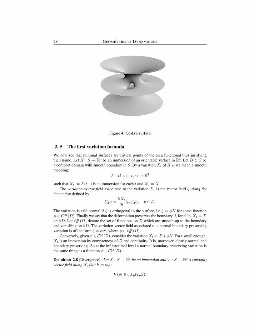
78 GEOMETRIES ET DYNAMIQUES
Figure 4: Costa’s surface
2. 5 The first variation formula
We now see that minimal surfaces are critical points of the area functional thus justifyingtheir name. Let X : S → R3 be an immersion of an orientable surface in R3. Let D ⊂ S bea compact domain with smooth boundary in S. By a variation Xt of X|D we mean a smoothmapping:
F : D × (−ε, ε)→ R3
such that Xt := F (t, .) is an immersion for each t and X0 = X.
The variation vector field associated to the variation Xt is the vector field ξ along theimmersion defined by:
ξ(p) =∂Xt
∂t|t=0(p), p ∈ D.
The variation is said normal if ξ is orthogonal to the surface, i.e ξ = φN for some functionφ ∈ C∞(D). Finally we say that the deformation preserves the boundary if, for all t, Xt = Xon ∂D. Let C∞0 (D) denote the set of functions on D which are smooth up to the boundaryand vanishing on ∂D. The variation vector field associated to a normal boundary preservingvariation is of the form ξ = φN, where φ ∈ C∞0 (D).
Conversely, given φ ∈ C∞0 (D), consider the variationXt = X+φN. For t small enough,Xt is an immersion by compactness of D and continuity. It is, moreover, clearly normal andboundary preserving. So at the infinitesimal level a normal boundary preserving variation isthe same thing as a function φ ∈ C∞0 (D).
Definition 2.8 (Divergence) LetX : S → R3 be an immersion and V : S → R3 a (smooth)vector field along X, that is to say:
V (p) ∈ dXp(TpS),

R. SOUAM 79
for all p ∈ S. For w ∈ TpS, denote by dV (w)⊥ the orhtogonal projection of dV (w) ondXp(TpS). The divergence of V, denoted div V is the trace of this map:
TS → TS
w → dV (w)⊥.
Otherwise said: for p ∈ S, let e1, e2 be an orthonormal basis of TpS, then
div V (p) = 〈dV (e1), dX(e1)〉+ 〈dV (e2), dX(e2)〉.
If now V is a vector field on S, then its divergence is by definition the divergence of dX(V ).
Let ω denote the area form of the surface X (see [15]). Recall that for w1, w2 ∈ TS, wehave
ω(w1, w2) = det(dX(w1), dX(w2), N).
Let V be a vector field along the immersion X, we define a 1-form iV ω as follows:
iV ω(w) = det(V, dX(w), N).
Proposition 2.9 d(iV ω) = (divV )ω.
Proof. We show the equation is verified at each point of S. Let p ∈ S and let (u, v) be localcoordinates in S around p compatible with the orientation. In these coordinates the 1-formiV ω writes:
iV ω = iV ω(Xu) du+ iV ω(Xv) dv = det(V,Xu, N) du+ det(V,Xv, N) dv.
So:
d(iV ω) =∂
∂udet(V,Xv, N)− ∂
∂vdet(V,Xu, N)
du ∧ dv.
We have:∂
∂udet(V,Xv, N) = det(Vu, Xv, N) + det(V,Xvu, N) + det(V,Xv, Nu)
= det(Vu, Xv, N) + det(V,Xvu, N),
because Nu is tangent to the surface. Similarily:
∂
∂vdet(V,Xu, N) = det(Vv, Xu, N) + det(V,Xuv, N).
Therefore:d(iV ω) = det(Vu, Xv, N)− det(Vv, Xu, N) du ∧ dv.
We may assume the coordinates (u, v) are such that the basis Xu, Xv is orthonormal andpositively oriented at p. This is always possible, take any coordinates and perform a linearchange of coordinates. Then at p we have:
d(iV ω)(p) = 〈Vu, Xu〉(p) + 〈Vv, Xv〉(p) det(Xu(p), Xv(p), N(p))du ∧ dv(p).
So:d(iV ω)(p) = divV (p)ω(p).

80 GEOMETRIES ET DYNAMIQUES
We are now in position to prove the:
Proposition 2.10 (The first variation formula) LetXt be a boundary preserving variation ofan immersion X : D → R3, where D is a compact orientable surface, oriented by a choiceof a unit normal field N. Call A(t) the area of Xt. Then:
dA
dt(0) = −2
∫D
φHdA,
where H is the mean curvature of the immersion and φ = 〈∂Xt∂t |t=0, N〉.
Proof. We denote by Nt the unit normal field associated to the immersion Xt and dependingsmoothly on t, with N0 = N and by dAt its area element. We have:
A(t) =∫D
dAt,
so we need to compute the derivative of the area element dAt. Let p ∈ D and let (u, v) belocal coordinates around p in S compatible with the orientation. Then:
dAt = det((Xt)u, (Xt)v, Nt) dudv.
Set N = dNtdt |t=0. We have:
d
dtdet((Xt)u, (Xt)v, Nt)|t=0 = det(ξu, Xv, N) + det(Xu, ξv, N) + det(Xu, Xv, N).
It follows from 〈Nt, Nt〉 = 1 that N is tangent to the surface and so the last term in theright-hand side of the previous equation vanishes. Write:
ξ = φN + V
where V is the tangent part to the immersion of the deformation vector field ξ. Then:
ξu = dφ(∂
∂u)N + φNu + Vu, ξv = dφ(
∂
∂v)N + φNv + Vv.
Therefore:
d
dtdet((Xt)u, (Xt)v, Nt)|t=0 = φ det(Nu, Xv, N) + det(Xu, Nv, N)
+det(Vu, Xv, N) + det(Xu, Vv, N).
Now as in the previous Propositon we may assume the basis Xu, Xv is orthonormal andpositive at the point p and so:
d
dtdet((Xt)u, (Xt)v, N)|t=0(p) = φ(p) 〈Nu, Xu〉(p) + 〈Nv, Xv〉(p)
+〈Vu, Xu〉(p) + 〈Vv, Xv〉(p)= 2φ(p)tr(dN(p)) + divV (p)= −2φ(p)H(p) + divV (p).

R. SOUAM 81
It follows that:dAtdt
(p) = −2φ(p)H(p) + divV (p) dA(p).
Since this is true for every p ∈ D, we conclude that:
dA
dt(0) =
∫D
−2φH + divV dA.
Since V = 0 on ∂D, the 1-form iV ω vanishes on ∂D. By Stokes’ theorem:∫D
divV dA =∫D
d(iV ω) =∫∂D
iV ω = 0,
which completes the proof.
Corollary 2.11 An immersion X : S → R3 is minimal if and only if for every variation Xt
of X with compact support, the derivative of the area A(t) vanishes at t = 0 :
dA
dt(0) = 0.
3 The Plateau problemLet Γ be a Jordan curve in Rn, i.e a continuous curve which is homeomorphic to the circleS1. The Plateau problem asks to find the surface of least area spanning Γ. The problem wassolved independently by Douglas and Rado, in 1930, for disk-type surfaces. In order toformulate the result, we introduce some notations: B = (u, v) ∈ R2, u2 + v2 ≤ 1 willdenote the closed unit disk in the Euclidean plane.
A map X : B → Rn is said to be piecewise C1 if it is continuous and if it is C1 except
along ∂B and along a finite number of regular C1−arcs and points inB . A continuous map
φ : ∂B → Γ is said to be monotone if it is such that if ∂B is traversed once in the positivedirection, then Γ is traversed once also in a given direction, although we allow arcs of ∂B tomap to single points of Γ. Otherwise said, a monotone map is a continuous map of degree±1such that for each p ∈ Γ, φ−1(p) is connected.
Let C(Γ) = X : B → Rn, X is piecewiseC1 andX|∂B is a monotone parameterizationof ΓWe define the area functionalA : C(Γ)→ R∪∞ by the following (maybe improper)integral:
A(X) =∫B
|Xu ∧Xv|dudv
where |Xu ∧Xv|2 = |Xu|2|Xv|2 − 〈Xu, Xv〉2. Let
AΓ = infX∈C(Γ)
A(X).
Therefore our problem is to find a X ∈ C(Γ) such that A(X) = AΓ.Note that we have to restrict ourselves to curves Γ satisfying AΓ < ∞ since there are
examples of Jordan curves bounding no surfaces of finite area. If Γ is rectifiable, for instanceC1, then it is true that AΓ <∞ (cf.[12]).

82 GEOMETRIES ET DYNAMIQUES
The idea is to try to apply the direct method of the calculus of variations, that is take asequenceXi ∈ C(Γ) such thatA(Xi)→ AΓ and try to extract a subsequence wich convergesto an X∞ ∈ C(Γ) with A(X∞) = AΓ. However this cannot work this way. The reason isthat the area functional is invariant under a big group of transformations: for any piecewiseC1 diffeomorphism ψ of the disk B, and any X ∈ AΓ we have A(X ψ) = A(X). We canfind a sequence of smooth homeomorphisms ψi of the unit disk B such that ψi(reiθ) →eiθ uniformly on compact subsets of B \ 0 and ψi(0) → 0. To get such an examplejust construct such a sequence of diffeomorphisms of the unit interval and then use polarcoordinates. Take for instance the sequence of homeomorphisms of the unit interval:
li(t) = t if 0 ≤ t ≤ 1i+1 ,
li(t) = (i2 − i− 1)t− i2−i−2i+1 if 1
i+1 ≤ t ≤1i ,
t+i−2i−1 if 1
i ≤ t ≤ 1,
which is piecewise smooth and perturb it a bit to make it smooth. Then assuming Xi con-verges uniformly to X∞ one can check that no subsequence of Xi ψi converges to a con-tinuous map.
So we need to control the parameterizations of our minimizing sequences. In the one-dimensional case, i.e curves in a Riemannian manifold, this is done by minimizing the energyintegral. Here minimizing sequences of curves tend to geodesics which not only minimizethe length integral but which are forced to be parameterized by a multiple of arc-length. Inthe case of surfaces the corresponding energy is the so-called Dirichlet integral:
D(X) =∫B
(|Xu|2 + |Xv|2)dudv.
Note that for any vectors v, w ∈ Rn we have:
|v ∧ w|2 = |v|2|w|2 − 〈v, w〉2 ≤ |v|2|w|2 ≤ 14
(|v|2 + |w|2)2,
and equality holds if and only if |v| = |w| and 〈v, w〉 = 0. Therefore, for any X ∈ C(Γ),
A(X) ≤ 12D(X)
with equality if and only if
|Xu| = |Xv| and 〈Xu, Xv〉 = 0
almost everywhere in B. Wherever |Xu| > 0, such a map is conformal and induces a metricon B of the form
ds2 = λ(du2 + dv2)
where λ = |Xu| = |Xv|. The parameters (u, v) are thus conformal coordinates for thesurface. A theorem of fundamental importance is the following:
Theorem 3.1 (Conformal representation of disk-type domains) Let X : B → Rn be a
continuous map such that X|B is an immersion of class Ck, 1 ≤ k ≤ ∞ (or real analytic).
Then there exists a homeomorphism ψ : B → B where ψ|B is of class Ck (or real analytic)
such that the parameterized mapping X ′ = X ψ is conformal.

R. SOUAM 83
Consider a Jordan curve Γ ⊂ Rn and define:
DΓ = infX∈C(Γ)
D(X).
Clearly:
AΓ ≤12DΓ.
Now take a sequence Xk ∈ C(Γ) such that A(Xk) → AΓ. The Xk are not necessarily im-mersions so we cannot apply directly the Theorem 3.1. The trick is to consider the sequenceof mappings: Xk : B → Rn+2, defined by
Xk(u, v) = (Xk(u, v),1ku,
1kv).
Clearly the Xk are C1−immersions (even embeddings) and so there exist homeomorphismsψk of B given by the Theorem 3.1 such that the Xk ψk are conformal. Using the invarianceof area under reparametrizations and some elementary estimates, we get:
DΓ ≤ D(Xk ψk) ≤ D(Xk ψk) = 2A(Xk ψk) = 2A(Xk) ≤ 2A(Xk) +4πk
and it follows thatAΓ =
12DΓ.
Corollary 3.2 Let Γ ⊂ Rn be a Jordan curve with AΓ <∞. Then for any X ∈ C(Γ),
D(X) = DΓ if and only if A(X) = AΓ and X is almost conformal.
Hence to solve the Plateau problem it is sufficient to find a map X ∈ C(Γ) which mini-mizes the Dirichlet integral. We will use the
Theorem 3.3 (Dirichlet’s Principle) Let φ : ∂B → Rn be a continuous map and define
C(φ) = X : B → Rn : X is piecewise C1 and X|∂B = φ
Assume that the numberDφ = inf
X∈CφD(X)
is finite. Then there exists a unique map Xφ ∈ C(φ) such that D(Xφ) = Dφ. The function
Xφ is harmonic inB and represents the solution to the boundary value problem ∆X =
0, X|∂B = φ.
We can thus consider a minimizing sequence Xk ∈ C(Γ), for the Dirichlet functional
satisfying, Xk is hamonic inB . Still we cannot extract a converging subsequence, the rea-
son is that the Dirichlet energy is invariant under the action of the group of conformal dif-feomorphisms of the disk B. Recall that the group G of conformal orientation preservingdiffeormorphisms of the disk:
G = g(z) = eiθ0a+ z
1 + az, a ∈ C, |a| < 1, θ0 ∈ R (14)

84 GEOMETRIES ET DYNAMIQUES
is not compact. Indeed take a sequence ak ∈ C, |ak| < 1, ak → 1, then the sequence in G,gk(z) = ak+z
1+akzconverges uniformly on compact subsets ofB\−1 to the constant 1. So we
need to normalize the mappingsX ∈ C(Γ). This is done by imposing a three-point condition:choose three distinct points p1, p2, p3 ∈ Γ and three distinct points z1, z2, z3 ∈ ∂B, anddefine
C∗(Γ) = X ∈ C(Γ) : X(zk) = pk, k = 1, 2, 3.By the invariance of the Dirichlet integral under G, we have that
infD(X), X ∈ C∗(Γ) = DΓ,
and thus we may solve the Plateau problem by minimizing in this smaller class. We thus takea minimizing sequence Xk ∈ C∗(Γ), we claim that the boundary values Xk|∂B : ∂B → Rnform an equicontinuous family. The key to this crucial result is the following
Lemma 3.4 (The Courant-Lebesgue lemma) Suppose X ∈ C0(B,Rn) ∩ C1(B,Rn) and
satisfiesD(X) ≤M (15)
for some M with 0 ≤ M < ∞. For each z0 ∈ ∂B and r > 0 we define Cr to be theintersection of B with the circle of radius r centered at z, and we denote by s the arc lengthparameter of Cr. Then for each 0 < δ < 1, there exists a number ρ with δ ≤ ρ ≤
√δ such
that ∫Cρ
|Xs|2ds ≤2M
ρ log( 1δ ). (16)
Proof. For 0 < δ < 1, consider the integral
I =∫ √δδ
∫Cr
|Xs|2dsdr ≤ D(X) ≤M,
and express I as
I =∫ √δδ
p(r)1rdr where p(r) = r
∫Cr
|Xs|2ds.
Then by the mean value theorem for the measure d(log r), there exists a number ρ ∈ [δ,√δ],
such that
I = p(ρ)∫ √δδ
d(log r) = p(ρ)12
log(1δ
).
Thus, p(ρ) ≤ 2M/ log( 1δ ) as claimed.
We can now prove the following:
Proposition 3.5 Let M be a constant > DΓ. Then the family of functions
F = X|∂B : X ∈ C?(Γ) and D(X) ≤M
is equicontinuous on ∂B. Thus, by Ascoli’s theorem F is compact in the topology of uniformconvergence.

R. SOUAM 85
Proof. For z ∈ ∂B and 0 < r < 1, denote by l(Cr) the length of the curve Cr defined in theLemma 3.4. It follows from the Schwarz inequality that
l(Cr)2 = (∫Cr
|Xs|ds)2 ≤ 2πr∫Cr
|Xs|2ds.
Let 0 < δ < 1 be a fixed number andX ∈ F . It follows from the Lemma 3.4 that there existsδ ≤ ρ ≤
√δ such that
l(Cr)2 ≤ 2Mlog( 1
δ ).
Let now ε > 0 be a given number. By an easy topological argument one sees that thereexists a number d > 0 such that for all p, q ∈ Γ with 0 < ||p − q|| < d, one of thetwo components of Γ \ p, q will have diameter < ε. (Recall that the diameter of a setS ∈ Rn is diam(S) = sup||p − q||, p, q ∈ S.) We now choose 0 < δ < 1 such that√
4πM/ log( 1δ ) < d and such that the disks of radius
√δ centered at z1, z2, z3 are pairwise
disjoint. We may assume without loss of generality that ε < mini6=j||pi − pj ||. Then forany z ∈ ∂B, there exists by the Lemma 3.4 a real δ ≤ ρ ≤
√δ such that l(Cρ) < d. ∂B
is now divided by Cρ into two arcs: a small arc A′ containing z and its complement A′′
containing two of the points z1, z2, z3. By the monotonicity of X|∂B, the images X(A′) andX(A′′) determine a partition of Γ into two arcs and since l(Cρ) ≤ d one of them has diameter< ε. However, since X(A′′) contains at least two of the points p1, p2, p3, its diameter is > ε.Hence, diameter (X(A′)) < ε. This immediately implies that for z, z′ ∈ ∂B, |z − z′| < δ,we have ||X(z) − X(z′)|| < ε and δ depends only on ε and the points z1, z2, z3, p1, p2, p3.This shows the equicontinuity of the family X(A′′)
Now by Ascoli’s theorem each sequence in X(A′′) has a convergent subsequence for theuniform convergence. To conclude note that a limit of monotone maps is also monotone.
Theorem 3.6 (Douglas, Rado) Let Γ be a Jordan curve in Rn such that AΓ < ∞. Thenthere exists a continuous map X : B → Rn such that
(1) X|∂B maps ∂B monotonically onto Γ,
(2) X|B is harmonic and almost conformal,
(3) D(X) = AΓ.
Proof. Let Xk ∈ C∗(Γ) be a minimizing sequence, limk→∞D(Xk) = DΓ. By the Theorem
3.3 we can assume theXk harmonic inB . By the Proposition 3.5, we can find a subsequence,
still denoted Xk, such that Xk|∂B converges uniformly to a monotone parametrization φ :∂B → Γ. Denote by Xφ the hamonic extension of φ to B given by the Dirichlet principle(Theorem 3.2). Then the maximum principle for harmonic functions ensures that Xk → Xφ
uniformly on B as k → ∞. Harnack’s principle ensures that ∇Xk → ∇Xφ as k → ∞uniformly on compact subsets of
B. Let then K be any compact subset of
B. Then:∫
K
|∇Xφ|2 = limk→∞
∫K
|∇Xk|2 ≤ lim infk→∞
D(Xk).

86 GEOMETRIES ET DYNAMIQUES
Letting K tend to B, we get:
D(Xφ) ≤ lim infk→∞
D(Xk) = DΓ.
The map X is called a classical solution to the Plateau problem for Γ.
Remark 3.1. The solution to Plateau’s problem obtained this way is a branched minimalsurface, i.e. a non constant continuous map X : B → Rn which is almost conformal andharmonic inside B. The Proposition 2.6, which easily extends to minimal surfaces in Rn,holds for such a map exactly as for immersed minimal surfaces except that the condition (10)is lacking. The points where the map is not an immersion are called its branch points. Theyare the zeroes of the holomorphic functions Φ1, . . . ,Φn and so are isolated. R. Ossermanproved that, for n = 3, the solution is free of branch points inside B (the proof was incom-plete and was completed by R. Gulliver). This is not the case for n ≥ 4, there are exampleswhere the solution has branch points. Another issue is the regularity at the boundary. Manyauthors contributed to settle the problem. For more information one may see [12] or [9] andthe references therein.
It remains to check that the classical solution to Plateau’s problem is a homeomorphismon ∂B. To see this we will need the following fact which is of independent interest:
Proposition 3.7 (The reflection principle) Let X : (u, v) ∈ R2, u2 + v2 < ε, v >0 −→ Rn be a branched minimal surface. Suppose there exists a line L in Rn such thatX(u, v)→ L when v → 0. Then X can be extended as a branched minimal surface definedin the whole disk (u, v) ∈ R2, u2 + v2 < ε by reflection across L.
Proof. We may assume, after a rotation in space, that L is the xn axis. By the reflectionprinciple for harmonic functions, the functions X1, X2 extend to harmonic functions on thewhole disk by setting Xk(u, 0) = 0, Xk(u, v) = −Xk(u,−v); k = 1, . . . , n − 1. Thus thefunctions
Φk =∂Xk
∂u− i∂Xk
∂v, k = 1, . . . , n− 1
are holomorphic on the whole disk and imaginary on the real axis. The equation:
Φ2n = −Φ2
1 − . . .− Φ2n−1,
shows Φn extends continuously to the real axis and takes nonnegative real values there.Therefore Φn extends continuously to the real axis and has real values there. By the re-flection principle for holomorphic functions, we can extend Φn to the whole disk by settingΦn(z) = Φn(z). IntegratingXn(z) = <e(
∫ z0
Φn(z)dz),we see thatXn extends to the wholedisk by the relation:
Xn(u, v) = Xn(u,−v).
We can now prove the following:

R. SOUAM 87
Proposition 3.8 For each solution X : B → Rn to the Plateau problem for Γ, the mapX|∂B : ∂B → Γ is a homeomorphism.
Proof. Since X|∂B −→ Γ is monotone, the only way it fails to be a homoeomorphism isthat it sends an arc of ∂B to a single point. Suppose this is the case. After a preliminaryconformal map ofB onto the upper half-plane we can apply the reflection principle (Proposi-tion 3.7) and extend the surface to a branched surface beyond a segment of the real axis. Thebranched surface thus obtained would send the whole segment to a point. This contradictsthe isolatedness of branch points of branched minimal surfaces (cf. Remark 3.1).
The solution to Plateau’s problem and the reflection principle give a way to constructcomplete surfaces. One may start with a polygonal curve and solve the Plateau problem andthen use the reflection principle to reflect the solution across the edges on the boundary. Onecan then do again reflections across the new boundary edges and so on. Of course the surfacemay be singular at the vertices of the initial boundary (and their images after reflections). Ifone chooses carefully the polygonal curve one can obtain a complete minimal surface whichis immersed everywhere. An example obtained starting from an appropiate quadrilateral inspace is a famous surface discovered by Schwarz (figure 5). It is triply periodic (i.e invariantunder three independent translations) and embedded.
The solution to Plateau’s problem gives a surface which minimizes area among disk-type surfaces. This does not mean the solution obtained has the smallest area among all thepossible surfaces bounded by the curve. The proof of the existence of a surface minimizingthe area among all possible surfaces without restriction on their topological type requiresthe techniques of geomeric measure theory. This is a difficult but very powerful theory forestablishing existence and regularity of volume minimizing submanifolds and applies to moregeneral manifolds. A readable introduction to this subject is [11].
Figure 5: The Schwarz surface

88 GEOMETRIES ET DYNAMIQUES
4 The stability of minimal surfaces
4. 1 The second variation formulaWe are now interested in the second derivative of the area functional for minimal surfaces inorder to study those which are minimizing up to the second order. It is not true in general thata minimal surface minimizes the area with respect to its boundary even among neighbooringsurfaces. We will see this happens for instance for some catenoid slices as a consequenceof the discussion to follow. However it can be proved that each point on a minimal surfaceadmits a neighborhood which is minimizing with respect to its boundary.
We will now derive the second variation formula. We first need to recall some definitions.
Definition 4.1 (The gradient and the Laplacian) Let (S, 〈, 〉) be a Riemannian surface andf : S → R a C1 function on S. The gradient of f, denoted ∇f, is the vector field on S suchthat:
〈∇f(p), w〉p = dfp(w),
for every p ∈ S and w ∈ TpS.Let f ∈ C2(S). The Laplacian of f, denoted ∆f, is the function defined by:
∆f = div(∇f).
With this definition, the Laplacian on the plane for the Euclidean metric ds20 = du2 +dv2
is ∆0 = ∂2
∂u2 + ∂2
∂v2 . If the metric on a surface S is given in conformal coordinates by:
ds2 = λ2(du2 + dv2),
then the associated Laplacian is related to the Euclidean Laplacian as follows:
∆ =1λ2
∆0. (17)
We can now state the second variation formula. To simplify the presentation, we restrictourselves to normal variations, however the same formula holds in the general case.
Proposition 4.2 (The second variation formula) Let Xt be a normal boundary preservingvariation of a minimal immersion X : D → R3, where D is a compact orientable surface,oriented by a choice of a unit normal field N. Call ξ the deformation vector field of Xt andset φ = 〈ξ,N〉. Then the second derivative of the area is:
d2A
dt2(0) = −
∫D
φ∆φ− 2Kφ2dA
=∫D
|∇φ|2 + 2Kφ2dA.
Proof. The second equality follows from Stokes’ theorem and the esaliy checked identity:
div(φ∇φ) = |∇φ|2 + φ∆φ.

R. SOUAM 89
Denote by Nt the unit normal field to the immersion Xt depending smoothly on t, withN0 = N and let Ht and dAt be respectively the mean curvature and the area element of Xt.Finally put: ξt = ∂Xt
∂t |t.By the first variation formula (Proposition 2.10), for each t:
dA
dt(t) = −2
∫D
〈ξt, Nt〉Ht dAt.
Taking into account that the immersion X is minimal, i.e H0 = 0, we get:
d2A
dt2(0) = −2
∫D
φdHt
dt|t=0 dA.
It remains to compute dHtdt |t=0. We first compute the derivative N = dNt
dt |t=0. Let p ∈ S and(u, v) local coordinates around p such that the basis Xu, Xv is orthonormal at p. For eacht we have:
〈Nt, (Xt)u〉 = 〈Nt, (Xt)v〉 = 0,
so taking the derivatives:〈N ,Xu〉 = −〈N, ξv〉,〈N ,Xv〉 = −〈N, ξu〉.
Now, ξu = (φN)u = dφ( ∂∂u )N + φNu and ξv = (φN)v = dφ( ∂∂v ) + φNv. So:
〈N ,Xu〉 = −dφ(∂
∂u),
〈N ,Xv〉 = −dφ(∂
∂v).
Moreover since 〈Nt, Nt〉 = 1 we have: 〈N ,N〉 = 0. It follows that at the point p :
N(p) = −∇φ(p).
Since this is true for every p ∈ S, we conclude that:
N = −∇φ (18)
Denote by Bt the shape operator of the immersion Xt, i.e the field of endomorphisms ofTS defined by:
It(Btw1, w2) = IIt(w1, w2),
which means:〈dXt(Btw1), dXt(w2)〉 = −〈dNt(w1), dXt(w2)〉.
Put B = dBtdt |t=0. Taking the derivatives at t = 0 :
〈dξ(Bw1) + dX(Bw1), dX(w2)〉+ 〈dX(Bw1), dξ(w2)〉 = −〈d(N)(w1), dX(w2)〉−〈dN(w1), dξ(w2)〉.

90 GEOMETRIES ET DYNAMIQUES
Writing ξ = φN and using (18), we obtain after simple calculations:
φ〈dN(Bw1), dX(w2)〉+ 〈dX(Bw1), dX(w2)〉+ φ〈dX(Bw1), dN(w2)〉 == 〈d(∇φ)(w1), dX(w2)〉 − φ〈dN(w1), dN(w2)〉.
Finally:
〈dX(Bw1), dX(w2)〉 = 〈d(∇φ)(w1), dX(w2)〉+ φ〈dX(Bw1), dX(Bw2)〉.
Take any point p ∈ S and a basis e1, e2 of TpS formed of principal eigenvectors withassociated principal curvatures k and −k (remember the surface is minimal). It follows that:
2dHt
dt|t=0(p) = tr(B)(p)
= 〈dX(Be1), dX(e1)〉+ 〈dX(Be2), dX(e2)〉= div(∇φ)(p) + 2k2φ(p).
This is true for any p ∈ S, so finally:
2dHt
dt|t=0 = ∆φ− 2Kφ.
A deformation Xt of an immersion is said trivial if Xt = X, for every t.
Definition 4.3 A compact domain D ⊂ S on a minimal immersion X : S → R3 is saidstable if for every nontrivial normal boundary preserving variation Xt on D :
d2A
dt2(0) > 0.
Equivalently: ∫D
|∇φ|2 + 2Kφ2dA > 0,
for all φ ∈ C∞0 (D), φ not identically 0.
This definition means that the domain is minimizing up to the second order for boundarypreserving variations. For instance, a domain on a plane is clearly stable since the curvaturevanishes identically.
4. 2 The Barbosa-do Carmo stability criterionThe Barbosa-do Carmo theorem ([2]) gives a nice and easy to verify criterion for the stabilityof minimal surfaces.
Theorem 4.4 (The Barbosa-do Carmo stability theorem) Let D be a regular compact do-main on a minimal surface. Assume the area of the Gaussian image N(D) on the sphere isless than 2π. Then D is stable.

R. SOUAM 91
To prove the theorem we need to recall some basic facts about the fundamental Dirichlet-eigenvalue of Schrodinger operators on surfaces. These notions make sense on Riemannianmanifolds of any dimension but we will restrict ourselves to the two-dimensional case. Moredetails can be found in [3] and [5].
Proposition 4.5 Let S be a Riemannian surface, q ∈ C∞(S) a smooth function on S andΩ ⊂ S an open regular domain with compact closure in S. Then the operator ∆ + q has adiscrete spectrum for the Dirichlet eigenvalue problem on Ω. The eigenfunctions are smoothup to the boundary of Ω. The first eigenvalue λ1(∆ + q,Ω) is simple and is characterized bythe property:
λ1(∆ + q,Ω) = inff∈C2
0 (Ω), f 6=0
∫Ω|∇f |2 − qf2 dA∫
Ωf2 dA
. (19)
Moreover the associated nontrivial eigenfunctions realize the infimum in (19) and arecharacterized, among other eigenfunctions, by the fact that they do not vanish inside D.
Furthermore, the first eigenvalue enjoys a monotonicity property: if Ω ⊂ Ω′ ⊂ S are twoopen regular domains with compact closure and Ω 6= Ω′, then:
λ1(∆ + q,Ω) > λ1(∆ + q,Ω′).
Let us find for instance the fundamental eigenvalue of the Laplacian on a hemisphereon S2. We denote by ∆1 the Laplacian on S2. It suffices to consider the hemisphere S2
+ =(x1, x2, x3) ∈ S2, x3 ≥ 0. Then since S2 has mean curvature −1 with respect to the out-ward unit normal,the restriction h of the coordinate function x3 to S2 satisfies (cf. Proposition2.4 and (17)):
∆1h+ 2h = 0 in S2+,
h = 0 on ∂S2+.
The Proposition 4.5 then shows:λ1(∆1,S2
+) = 2. (20)
We will need the following result:
Theorem 4.6 (Faber-Krahn) Let Ω be a regular domain on the unit sphere S2 and let Ω? bea round disk having the same area as Ω. Then:
λ1(∆1,Ω) ≥ λ1(∆1,Ω?)
with equality if and only if Ω is a round disk.
This theorem was proved by Faber and Krahn in the Euclidean case but the proof extendsto the spherical case (and to the hyperbolic one too). For the proof see [3] or [5].
The Theorem 4.6, the monotonicity property (cf. Proposition 4.5) and (20) then give the:
Corollary 4.7 Let Ω be a domain in S2. Assume the area of Ω is less than 2π. Then:
λ1(∆1,Ω) > 2.

92 GEOMETRIES ET DYNAMIQUES
We now use the following result due to D. Fischer-Colbrie and R. Schoen [6] (whichholds in any dimension). We give an independent proof.
Lemma 4.8 Consider a Riemannian surface S and denote by ∆ the associated Laplacian.Let q be a smooth function on S andD ⊂ S be a compact domain in S with smooth boundary.Assume there exists a function u ∈ C2(D) ∩ C0(D) satisfying:
∆u+ qu ≤ 0 in D and u > 0 on D.
Then λ1(∆ + q,D) > 0.
Proof. Set w = ∆u + qu. Let h ∈ C∞0 (D), since u > 0 we can write: h = ψu withψ ∈ C2
0 (D). Using Stokes’ formula, we can write:
∫D
|∇h|2dA = −∫D
h∆h dA = −∫D
ψu∆(ψu)dA
= −∫D
ψu(u∆ψ + ψ∆u+ 2〈∇u,∇ψ〉)dA
= −∫D
ψu2∆ψ + ψ2u(w − qu) + 2uψ〈∇u,∇ψ〉dA
So:∫D
|∇h|2 − qh2dA = −∫D
ψu2∆ψ + 2uψ〈∇u,∇ψ〉dA−∫D
ψ2uwdA
≥ −∫D
ψu2∆ψ + 2uψ〈∇u,∇ψ〉dA.
Using again Stokes’ formula:∫D
ψu2∆ψ dA =∫D
div(ψu2∇ψ)− 〈∇(ψu2),∇ψ〉 dA
= −∫D
〈∇(ψu2),∇ψ〉 dA
= −∫D
2uψ〈∇u,∇ψ〉+ u2|∇ψ|2dA.
Therefore: ∫D
|∇h|2 − qh2dA ≥∫D
u2|∇ψ|2dA ≥ 0.
Moreover if the leftmost-hand side vanishes thenψ is constant and soψ = 0 (sinceψ vanisheson ∂D) and thus also h = 0. We conclude then by the characterization (19).
Proof of Barbosa-do Carmo’s theorem. As we observed above, a domain on a plane is stable,so we will assume our domain does not lie on a plane. We will prove the existence of functionu ∈ C2(D) ∩ C0(D), which is positive on D and satisfying: ∆u − 2Ku ≤ 0. The Lemma

R. SOUAM 93
4.8 will then imply that λ1(∆− 2K,D) > 0, where ∆ is the Laplacian for the metric ds2 onthe surface. Taking into account the Proposition 4.8, this then means D is stable.
Set Ω = N(D) ⊂ S2. Since N is conformal and non constant, Ω is an open set withpiecewise smooth boundary. By hypothesis area(Ω) < 2π.We may consider an open domainΩ with smooth boundary such that Ω ⊂ Ω and area(Ω) < 2π. By the Corollary 4.7 we have:
λ1(∆1, Ω) > 2.
Let v a nontrivial eigenfunction associated to λ1(∆1, Ω).We may assume v > 0 inside Ω (cf.Proposition 4.5). Then for the spherical Laplacian ∆1, we have:
∆1v + 2v < ∆1v + λ1(∆1, Ω)v = 0 in Ω and v > 0 on Ω.
On the set D0 = D − K = 0, the Gauss map is a local diffeomorphism, so we mayconsider the pull-back metric
ds22 = N∗ds2
1.
For the Laplacian ∆2 associated to ds22, there holds the relation:
∆2(v N) = ∆1v.
It follows that the function u := v N : D → R satisfies on D :
∆2u+ 2u < 0.
Furthermore, since N is conformal, we have:
ds22 = N∗ds2
1 = −Kds2.
It is straightforward to check the relation between the Laplacians:
∆2 =∆
(−K).
It follows (since K < 0) that u satisfies:
∆u− 2Ku < 0 in D0.
It follows from (13) that on a nonplanar minimal surface the zeroes of the Gaussian curvatureare isolated. Therefore we have by continuity:
∆u− 2Ku ≤ 0 in D.
Moreover, by construction, the function u is positive on D.
Remark 4.1. As it should be clear, the proof shows more generally that if the first eigenvalueof the Gaussian image N(D) for the Laplacian with Dirichlet condition is bigger then 2 thenthe domain D is stable. This is the case for instance if area(N(D)) = 2π and N(D) is not ahemisphere.

94 GEOMETRIES ET DYNAMIQUES
Corollary 4.9 Let D be a regular domain on a minimal surface in R3. Assume:∣∣∣∣∫D
K dA
∣∣∣∣ < 2π.
Then D is stable.
Proof. The Gauss map of a nonplanar minimal surface is an orientation reversing local diffeo-morphism except at isolated points which are the zeroes of the Gaussian curvature. Therefore:
area(N(D)) =∫N(D)
dA1 ≤∫D
N∗(dA1),
dA1 being the area element on S2. The area element dA of the surface is related to dA1 asfollows (cf. [15]): N∗dA1 = −KdA. Therefore:
area(N(D)) =∫N(D)
dA1 ≤∫D
N∗(dA1) =∫D
(−K)dA =∣∣∣∣∫D
K dA
∣∣∣∣and the result follows from Barbosa-do Carmo’s theorem.
It should be clear from the previous considerations that in case the Gauss map is injective,which happens for instance on the catenoid and Enneper’s surface, then stable domains areprecisely those having absolute total curvature less than 2π.
A question which naturally comes to mind is to determine the complete minimal surfaces(without boundary) which are globally stable. A complete minimal surface is said globallystable if all its compact subdomains are stable. For instance a plane is globally stable. Atheorem proved independently by do Carmo-Peng, Pogorelov and by Fischer-Colbrie andSchoen [6] states that the planes are the only globally stable complete (orientable) minimalsurfaces without boundary in R3.
References[1] J. Barbosa and G. Colares.: Minimal surfaces in R3. Translated from the Portuguese.
Lecture Notes in Mathematics, 1195. Springer-Verlag, Berlin, (1986).
[2] J.L. Barbosa and M.P. do Carmo.:On the size of a stable minimal surface in R3. Amer.J. Math. 98 (1976), no. 2, 515–528.
[3] M. Berger; P. Gauduchon and E. Mazet.: Le spectre d’une variete riemannienne. Lec-ture Notes in Mathematics, Vol. 194 Springer-Verlag, Berlin-New York, (1971).
[4] M. P. do Carmo.: Differential Geometry of Curves and Surfaces. Prentice-Hall Inc.,Englewood Cliffs,N.J., (1976).
[5] I. Chavel.: Eigenvalues in Riemannian geometry. Including a chapter by Burton Ran-dol. With an appendix by Jozef Dodziuk. Pure and Applied Mathematics, 115. Aca-demic Press, Inc., Orlando, FL, (1984).

R. SOUAM 95
[6] D. Fischer-Colbrie and R. Schoen. The structure of complete stable minimal surfacesin 3-manifolds of nonnegative scalar curvature. Comm. Pure Appl. Math. 33 (1980),no. 2, 199–211.
[7] D. Gilbarg and N.Trudinger.: Elliptic partial differential equations of second order.Grundlehren der Mathematischen Wissenschaften, Vol. 224. Springer-Verlag, Berlin-New York, (1977).
[8] D. Hoffman and H. Karcher,.:Complete embedded minimal surfaces of finite total cur-vature. Geometry, V, 5–93, 267–272, Encyclopaedia Math. Sci., 90, Springer, Berlin,(1997).
[9] H. B. Lawson.:Lectures on minimal submanifolds. Vol. I. Second edition. MathematicsLecture Series, 9. Publish or Perish, Inc., Wilmington, Del., (1980).
[10] F. Lopez and F. Martin.:Complete minimal surfaces in R3. Publ. Mat. 43 (1999), no.2, 341–449.
[11] F. Morgan.:Geometric measure theory. A beginner’s guide. Academic Press, Inc.,Boston, MA, (1988).
[12] R. Osserman.: A survey of minimal surfaces. Second edition Dover Publications, Inc.,New York, (1986).
[13] J. Perez and A. Ros.:Properly embedded minimal surfaces with finite total curvature.The global theory of minimal surfaces in flat spaces (Martina Franca, 1999), 15–66,Lecture Notes in Math., 1775, Springer, Berlin, (2002).
[14] H. Rosenberg.:Some recent developments in the theory of properly embedded minimalsurfaces in R3. Seminaire Bourbaki, Vol. 1991/92. Asterisque No. 206, (1992), Exp.No. 759, 5, 463–535.
[15] R. Souam.: Basic geometry of curves and surfaces. These proceedings.
Rabah SouamInstitut de Mathematiques de Jussieu - CNRS UMR 7586Universite Paris Diderot - Paris 7, ”Geometrie et Dynamique”Case 7012 75205 - Paris Cedex 13e-mail: [email protected]


Deuxieme partie
Espaces Homogenes
97


Produits scalairespseudo-euclidiens
par
BENOIT KLOECKNER
Les produits scalaires pseudo-euclidiens forment le modele ponctuel des geometries rie-manniennes et pseudo-riemanniennes. Apres en avoir developpe les proprietes elementaireson se propose d’etudier deux aspects lies a la geometrie pseudo-riemannienne : l’orientationdu temps en signature lorentzienne et la caracterisation de l’equivalence conforme par lescones isotropes.
On se place dans toute la suite sur un espace vectoriel reel E dont la dimension est sup-posee finie et notee n.
1 Formes bilineaires et quadratiques
1. 1 DefinitionDefinition 1.1 Une application φ : E × E → R est appelee forme bilineaire symetrique sielle est lineaire en chacune de ses variables et verifie
φ(x, y) = φ(y, x) ∀x, y ∈ E. (1)
Soit φ une forme bilineaire symetrique sur E. On definit sur E une fonction Qφ par
Qφ(x) = φ(x, x) ∀x ∈ E. (2)
On dit que Qφ est la forme quadratique associee a φ et que φ est la forme polaire de Qφ.Comme φ et Qφ sont relies par l’identite de polarisation
φ(x, y) =14
(Qφ(x+ y)−Qφ(x− y)) ∀x, y ∈ E (3)
il y a unicite de la forme polaire.
99

100 GEOMETRIES ET DYNAMIQUES
Exemple 1. (1) Le produit scalaire canonique((x1, . . . , xn); (y1, . . . , yn)
)7→ x1y1 + x2y2 + · · ·+ xnyn
est une forme bilineaire symetrique sur Rn dont la forme quadratique est :
(x1, . . . , xn) 7→ x21 + · · ·+ x2
n.
(2) L’application ((x1, x2); (y1, y2)
)7→ x1y2 + y1x2
en est une sur R2 qui a un comportement bien different : sa forme quadratique estdonnee par Q
((x1, x2)
)= 2x1x2, certains vecteurs ont donc une image nulle ou
negative.
(3) La figure 1 represente les lignes de niveau (Q = constante) d’une forme quadratiqueQ dite Lorentzienne (voir la section 4 pour une definition).
FIG. 1 – Exemple de forme quadratique
1. 2 Representation matricielleDefinition 1.2 Soit φ une forme bilineaire symetrique et B = (e1, . . . , en) une base de E.On note φi,j = φ(ei, ej). On appelle matrice de φ dans la base B et on note Mφ
B la matricen× n dont les coefficients sont les φi,j .

B. KLOECKNER 101
Comme φ est symetrique, sa matrice MφB l’est egalement.
Si X et Y sont les vecteurs colonnes de Rn exprimant les coordonnees dans la base B devecteurs x =
∑xiei, y =
∑yiei de E, la bilinearite de φ entraıne :
φ(x, y) = tXMφBY =
∑i,j
φi,jxiyj . (4)
donc MφB determine entierement φ. C’est la seule matrice verifiant (4) pour tous les couples
de vecteurs de E.Soit B′ = (e′1, . . . , e
′n) une autre base de E, P ∈ GL(n,R) la matrice de changement de
base de B a B′ et X ′ les coordonnees de x dans B′, de sorte que X = PX ′.On a alors φ(x) = tXMφ
BY = tX ′ tPMφBPX
′ donc :
MφB′ = tPMφ
BP. (5)
Ainsi, le rang de MφB ne depend pas de B.
Le determinant de MφB , lui, depend de B mais pas son signe (∈ −1, 0, 1) que l’on
appelle parfois discriminant de φ.L’expression (4) montre qu’une forme quadratique est toujours (et en toute base) un po-
lynome homogene de degre 2 en les coordonnees du vecteur considere.Inversement, l’identite de polarisation (3) permet de voir que tout polynome homogene
de degre 2 est une forme quadratique.
2 Produits scalaires
2. 1 DefinitionDefinition 2.1 Soit φ une forme bilineaire symetrique sur E dont on note Q la formequadratique. On dit que φ est :
– positive [resp. negative] si Q(x) > 0 [resp. 6 0] pour tout x ∈ E ;– definie positive [resp. definie negative] si Q(x) > 0 [resp. < 0] pour tout x 6= 0 ;– non degeneree si aucun vecteur x 6= 0 ne verifie : ∀y ∈ E, φ(x, y) = 0.
On appelle produit scalaire (pseudo-euclidien) une forme bilineaire symetrique non dege-neree.
Voir les figures 1 et 2 pour des exemples.On appelle produit scalaire euclidien un produit scalaire qui est defini positif. Dans la
litterature, la terminologie peut varier, il est donc important de noter qu’ici « produit scalaire »signifie seulement « forme bilineaire symetrique non degeneree ».
Soit φ une forme bilineaire symetrique sur E.On dit que φ est definie si elle est definie positive ou definie negative, qu’elle est semi-
definie si elle est positive ou negative.Il faut noter que φ est non degeneree si et seulement si elle est de rang n, i.e. si son
discriminant est non nul. Si φ est definie, elle est necessairement non degeneree.Si φ est definie, positive ou negative, et si F est un sous-espace de E, la restriction de φ a
F×F notee φ|F garde cette propriete. Mais si φ est non degeneree, il peut tres bien exister un

102 GEOMETRIES ET DYNAMIQUES
FIG. 2 – Une forme quadratique definie positive (a gauche) et une forme degeneree (a droite)
sous-espace F deE tel que φ|F soit degeneree (il y en a meme toujours si φ n’est pas definie :la droite engendree par un vecteur x non nul verifiant Q(x) = 0 en est un exemple). Ainsi unproduit scalaire non euclidien n’induit pas un produit scalaire sur tous les sous-espace de E.On introduit en consequence la terminologie suivante.
Definition 2.2 On dit d’un sous-espace sur lequel la restriction de φ est non degenereequ’il est non degenere.
De meme, on dit d’un espace sur lequel la restriction de φ est definie positive, definienegative, positive ou negative qu’il est lui-meme respectivement defini positif, defini negatif,positif ou negatif.
Voir les figures 3 et 4.
FIG. 3 – Un sous-espace non degenere (a gauche) et un sous-espace defini positif (a droite)
Les inegalites euclidiennes classiques, de Cauchy-Schwarz φ(x, y)2 6 Q(x)Q(y) et tri-

B. KLOECKNER 103
angulaire Q(x + y)1/2 6 Q(x)1/2 + Q(y)1/2, se prolongent au cas positif. L’inegalite deCauchy-Schwarz est egalement vraie dans le cas negatif, mais est toujours fausse si φ n’estni positive ni negative. L’inegalite triangulaire n’a pas de sens si Q n’est pas positive mais onpeut considerer sa generalisation naturelle |Q(x+ y)|1/2 6 |Q(x)|1/2 + |Q(y)|1/2. Celle-ciest vraie si Q est negative, mais elle est toujours fausse si Q n’est ni positive ni negative.
2. 2 Orthogonalite et isotropieDefinition 2.3 Soit φ une forme bilineaire symetrique sur E et x, y des vecteurs. On dit quex et y sont orthogonaux et on note x ⊥ y si φ(x, y) = 0.
Un vecteur est dit isotrope s’il est orthogonal a lui meme, c’est a dire s’il verifie Q(x) =0.
L’ensemble des vecteurs isotropes est appele cone isotrope de φ.L’ensemble des vecteurs orthogonaux a tous les vecteurs de E est appele le noyau de φ.
La relation d’orthogonalite est bien entendu symetrique.Le cone isotrope est reduit a 0 si et seulement si φ est definie. Le noyau est reduit a 0 si
et seulement si φ est non degeneree.
Definition 2.4 Soient F et G des sous-espaces de E. On dit que F et G sont orthogonauxet on note F ⊥ G si tout vecteur de l’un est orthogonal a tous les vecteurs de l’autre.
On appelle orthogonal de F et on note F⊥ l’ensemble des vecteurs de E qui sont ortho-gonaux a tous les vecteurs de F .
On dit de F qu’il est totalement isotrope s’il est inclus dans le cone isotrope.
FIG. 4 – Un plan et sa droite orthogonale (a gauche), un plan degenere et sa droite orthogonale(a droite)
Le noyau de φ n’est rien d’autre que E⊥.La bilinearite de φ fait de l’orthogonal de F un sous-espace vectoriel de E, mais en
general ce n’est pas un supplementaire de F . On garde tout de meme du cas euclidien leresultat suivant.

104 GEOMETRIES ET DYNAMIQUES
Proposition 2.5 Si φ est un produit scalaire et si F est un sous-espace de E, on a :
dimF + dimF⊥ = n et(F⊥)⊥
= F.
Demonstration. Considerons une base (e1, . . . , ek) de F que l’on complete en une base(e1, . . . , en) de E. Un vecteur
∑xiei de E est orthogonal a F si et seulement s’il verifien∑j=1
φi,jxj = 0 ∀ 1 6 i 6 k
qui est un systeme lineaire de rang k car φ etant non degenere sa matrice est inversible. Doncla dimension de F⊥ est n− k ou k est la dimension de F .
Il est clair que F ⊥ F⊥, donc F ⊆(F⊥)⊥
. Mais
dim(F⊥)⊥
= n− (n− dimF ) = dimF
donc en fait F =(F⊥)⊥
.
Lemme 2.6 Soit φ un produit scalaire surE et F un sous-espace. Alors F est non degeneresi et seulement si E = F ⊕ F⊥. De plus F est non degenere si et seulement si F⊥ l’est.
Demonstration. Comme dimF+dimF⊥ = n,E = F⊕F⊥ si et seulement si F ∩F⊥ = 0,donc si et seulement si il n’y a aucun vecteur non nul de F orthogonal a tous les vecteurs deF , ce qui est la definition d’un sous-espace non-degenere.
Enfin, comme(F⊥)⊥ = F , F est non degenere si et seulement si F⊥ l’est.
2. 3 Bases orthonormalesSoit φ une forme bilineaire. On appelle carre de x le nombreQ(x) = φ(x, x). On appelle
norme de x le nombre |φ(x, x)|1/2. Cette appellation est abusive, puisqu’en general ce n’estpas une norme. Un vecteur est unitaire s’il est de norme 1.
On dit d’une famille de vecteurs de E qu’elle est orthogonale si les vecteurs qui la com-posent sont deux a deux orthogonaux. Si φ est un produit scalaire et si de plus les vecteurssont unitaires, on dit que la famille est orthonormale.
Dans le cas pseudo-euclidien, on voit facilement qu’une famille orthonormale est toujourslibre. Ainsi on appelle base orthonormale de E une famille orthonormale a n elements.
Proposition 2.7 Tout produit scalaire admet une base orthonormale.
Demonstration. Soit φ un produit pseudo-euclidien. Comme φ est une forme bilineaire nondegeneree, il existe un vecteur e1 tel que φ(e1, e1) 6= 0. Quitte a remplacer e1 par un de sesmultiples, on peut supposer que e1 est unitaire.
Raisonnons par recurrence sur la dimension n de E. Si E est de dimension 1, (e1) enest une base, orthonormale pour φ. Si E est de dimension au moins 2, comme l’espace 〈e1〉engendre par e1 est non degenere, d’apres le lemme 2.6 l’espace 〈e1〉⊥ est non-degenere etE = 〈e1〉⊕〈e1〉⊥. Alors φ|〈e1〉⊥ est un produit pseudo-euclidien de dimension n−1. Par hy-pothese de recurrence il existe une base orthonormale (e2, . . . , en) de 〈e1〉⊥, et (e1, . . . , en)est une base orthonormale de E.

B. KLOECKNER 105
De la meme maniere, on voit que toute famille orthonormale peut etre completee en unebase orthonormale car elle engendre un sous-espace non degenere.
Soit (e1, . . . , en) une base orthonormale pour φ. La matrice de φ dans cette base a pourcoefficients φi,j = φ(ei, ej) = δji εj ou δ est le symbole de Kronecker (δji vaut 1 si i = j et0 sinon) et εj = φ(ej , ej) = ±1. Elle est donc diagonale et tous ses coefficients diagonauxvalent plus ou moins 1.
On note p le nombre de 1 et q le nombre de −1 qui apparaissent parmi les εj . Le couple(p, q) est appele signature de φ.
Lemme 2.8 La signature de φ est bien definie, c’est-a-dire ne depend pas de la base ortho-normale consideree.
Demonstration. Supposons qu’il existe une base orthonormee (e′1, . . . , e′n) pour laquelle φ a
une signature (p′, q′) 6= (p, q).Comme p+ q = p′+ q′ = n, on aurait p′ > p ou q′ > q. Quitte a considerer −φ, on peut
supposer p′ > p.Alors il existe un sous-espace E′+ de dimension p′ sur lequel φ est definie positive et un
sous-espaceE− de dimension n−p sur lequel φ est definie negative. Comme p′+n−p > n,necessairement E′+ ∩ E− 6= 0. Il existe donc un vecteur x tel que φ(x, x) est a la foisstrictement positif et strictement negatif, ce qui est absurde.
Finalement, ce qui precede permet d’etablir le resultat suivant.
Theoreme 2.9 Soit φ un produit pseudo-euclidien. Alors il existe une unique paire d’entiers(p, q), appelee signature de φ, telle qu’il existe une base B de E dans laquelle la matrice deφ soit
Ip,q =(Ip 00 −Iq
)(6)
ou Ik designe la matrice unite de dimension k.
On parle aussi de la signature d’une forme quadratique pour designer la signature de saforme polaire.
Remarque 2.1. On s’est limite au cas non degenere, mais on pourrait enoncer un resultatsimilaire pour une forme bilineaire symetrique quelconque : il existe une base dans laquellesa matrice est diagonale avec des coefficients diagonaux egaux a 1, −1 ou 0. La signaturecomporte alors trois nombres p, q, r donnant respectivement le nombre de 1, de −1 et de 0sur la diagonale. Le rang de la forme bilineaire consideree est p+q et c’est un produit scalairesi et seulement si r = 0.
La figure 1 montre une forme quadratique de signature (2, 1). La figure 2 montre uneforme de signature (1, 1, 1) et une forme de signature (3, 0). La figure 5 montre une forme designature (0, 1, 2) et une forme de signature (2, 0, 1).
2. 4 Traduction dans l’ecriture polynomialeSoit φ un produit scalaire, Q sa forme quadratique, (ei)i une base orthonormale. On note
comme precedemment εi = Q(ei) = ±1.

106 GEOMETRIES ET DYNAMIQUES
FIG. 5 – Deux formes semi-definies definies degenerees (signature (0, 1, 2) a gauche, (2, 0, 1)a droite)
Pour tout vecteur x ∈ E et pour tout indice j on a φ(x−∑εiφ(x, ei)ei, ej) = 0. Comme
φ est non degenere on en deduit
x =n∑i=1
εiφ(x, ei)ei. (7)
Ainsi on a
Q(x) =n∑i=1
εiφ(x, ei)2 (8)
et on voit que la forme quadratique de φ s’ecrit sous la forme Q =∑±l2i ou les li forment
une base du dual E∗ de E. Autrement dit, il existe une base de E dans laquelle on peut ecrireQ(x) =
∑±x2
i ou les xi sont les coordonnees de x dans la base en question.Donnons une methode pratique pour etablir une telle ecriture a partir de la donnee de
Q. Dans une base B = (ei)i quelconque, on peut ecrire Q(x) sous la forme d’un polynomehomogene de degre 2 en (x1, . . . , xn), les coordonnees de x dans B.
Si Q(x) admet un terme carre, de la forme ax2i , on ecrit (en se placant dans le cas i = 1
pour simplifier l’ecriture)
Q(x) = ax21 + x1P1(x2, . . . , xn) +Q′(x2, . . . , xn)
ou P1 est un polynome homogene de degre 1 donc represente une forme lineaire et Q′(x) estun polynome homogene de degre 2 en x2, . . . xn donc represente une forme quadratique surl’espace engendre par e2, . . . , en. On ecrit ensuite
Q(x) =a
|a|
(√|a|x1 +
√|a|
2aP1(x2, . . . , xn)
)2
− 14aP1(x2, . . . , xn)2 +Q′(x2, . . . , xn)
B. KLOECKNER 107
ou on observe que a|a| = ±1,
√|a|x1 +
√|a|
2a P1(x2, . . . , xn) est une forme lineaire sur E,− 1
4aP1(x2, . . . , xn)2 + Q′(x2, . . . , xn) est une forme quadratique sur le sous-espace en-gendre par e2, . . . , en. Il suffit ensuite d’iterer le procede.
SiQ(x) n’admet pas de terme carre et est non nul, il admet un terme rectangle de la formebxixj . On effectue alors le changement de variable y = xi+xj
2 , z = xi−xj2 , ce qui revient a
se placer dans la base obtenue a partir de B en remplacant ei par ei + ej et ej par ei − ej .L’expression deQ(x) dans la nouvelle base presente alors un terme carre by2 et on est rameneau cas precedent.
On obtient bien une famille libre de formes lineaires, car dans la base duale de B elles’ecrit de facon etagee (la premiere forme est la seule a dependre de x1, les deux premieressont les seules a dependre de x1 et x2, etc.)
Cette methode fonctionne sans utiliser l’hypothese de non degenerescence, et permetdonc de demontrer la remarque du theoreme 2.9.
2. 5 Interpretation de la signatureDans cette section on ne parle que de produits scalaire, mais on dispose de resultats ana-
logues dans le cas degenere.
Definition 2.10 On dit que deux produits scalaires φ1 et φ2 sur des espaces vectoriels E1
et E2 sont isometriques s’il existe un isomorphisme b : E1 → E2 qui envoie l’un sur l’autre,c’est-a-dire tel que pour tout couple (x, y) ∈ E2
1 on ait φ1(x, y) = φ2(b(x), b(y)).
D’apres le theoreme 2.9, deux produit scalaires sont isometriques si et seulement si ils ontmeme signature. La signature traduit donc completement les proprietes d’un produit scalaire ;par exemple le discriminant de φ vaut (−1)q . Des signatures opposees (p, q) et (q, p) sontsemblables puisque si l’une est la signature de φ, l’autre est celle de −φ. En general on secontente donc d’etudier le cas ou p > q.
Proposition 2.11 Soit φ un produit scalaire de signature (p, q). Alors il est defini positif siet seulement si q = 0, il est defini negatif si et seulement si p = 0.
Demonstration. Il suffit de voir que si p et q sont tous les deux non nuls, il existe necessaire-ment un vecteur isotrope. Or il existe alors deux vecteurs unitaires orthogonaux e+ et e− decarres respectifs 1 et −1. Alors e+ + e− est non nul et la bilinearite donne
φ(e+ + e−, e+ + e−) = φ(e+, e+) + 2φ(e+, e−) + φ(e−, e−)= 1 + 0− 1= 0
donc e+ + e− est isotrope.
Proposition 2.12 Soit φ un produit scalaire de signature (p, q). Alors p est la plus grandedimension possible pour un sous-espace defini positif, q est la plus grande dimension possiblepour un sous-espace defini negatif et min(p, q) est la plus grande dimension possible pourun espace totalement isotrope.

108 GEOMETRIES ET DYNAMIQUES
Demonstration. Il est facile en considerant une base orthonormee de voir qu’il existe un sous-espace defini positif de dimension p et un sous-espace defini negatif de dimension q. De pluss’il existait un sous-espace defini positif ou negatif de dimension plus grande, comme dans lademonstration du lemme 2.8 il existerait un vecteur de carre a la fois positif et negatif.
Pour les sous-espaces isotropes, on utilise la methode de la demonstration de la proposi-tion 2.11. Soit l = min(p, q). Une base orthonormale nous donne en particulier une familleorthonormale libre de vecteurs
(e+1 , e−1 , e
+2 , e−2 , . . . , e
+l , e−l )
ou les e+i sont de carre 1 et les e−i de carre −1. Alors la famille
(e+i + e−i )16i6l
est libre, orthogonale et formee uniquement de vecteurs isotropes. L’espace qu’elle engendreest donc totalement isotrope, de dimension l.
Maintenant s’il existait un espace totalement isotrope de dimension plus grande, il in-tersecterait non trivialement tout espace defini (negatif ou positif) de dimension maximale(> n − l) donc il existerait un vecteur de norme a la fois nulle et strictement positive ounegative.
3 Groupes orthogonauxEtant donne un produit scalaire φ sur E, on s’interesse au groupe O(φ) des endomor-
phismes qui preservent φ (on parle d’isometries).Remarquons que preserver φ est equivalent a preserver sa forme quadratique Q. L’une
des implications est evidente, l’autre decoule de l’identite de polarisation.Soit B une base de E et M la matrice de φ dans cette base. Alors si X et Y sont les
vecteurs coordonnees d’elements x et y de E, on a vu que φ(x, y) = tXMY . Soit b uneapplication lineaire de E dont on note B la matrice dans la base B. Alors b preserve φ si pourtous les couples de vecteurs de E on a φ(b(x), b(y)) = φ(x, y), autrement dit si tBMB =M .
D’apres le theoreme 2.9 il existe une base pour laquelle M = Ip,q ou (p, q) est lasignature de φ. Ceci justifie la definition suivante.
Definition 3.1 On note O(p, q) le groupe des matrices reelles carree B de dimension n (oun = p+ q) telles que
tBIp,qB = Ip,q (9)
On note SO(p, q) le groupe des matrices de O(p, q) dont le determinant vaut 1. On noteSO0(p, q) et on appelle groupe orthochrone la composante connexe de l’identite de O(p, q).
On definit de facon semblable SO(φ) et SO0(φ).L’equation (9) montre que O(p, q) ⊆ GL(n,R).On peut montrer (voir par exemple [1], chapitre 4) que si p et q sont non nuls, O(p, q)
est homeomorphe a O(p)×O(q)×Rpq . Il possede alors 4 composantes connexes. Grace au

B. KLOECKNER 109
theoreme 2.9 il est facile de voir que O(p, q) contient un sous-groupe isomorphe a O(p) ×O(q) et que SO0(p, q) contient un sous-groupe isomorphe a SO(p)× SO(q).
Comme dans le cas euclidien, on peut caracteriser les elements de O(p, q) par leur actionsur les bases.
Proposition 3.2 Soit (e1, . . . , en) une base de E orthonormale pour φ. Un endomorphismea de E est une isometrie si et seulement s’il envoie (e1, . . . , en) sur une base orthonormalepour φ en respectant le carre de ses elements (Q(a(ei)) = Q(ei) pour tout i).
Demonstration. Il suffit de considerer l’ecriture matricielle : l’action d’un endomorphismecorrespond exactement a un changement de base.
On deduit de ce resultat une consequence importante : l’action de O(φ) est transitive surles surfaces de niveau de Q, c’est-a-dire qu’etant donnes deux vecteurs non nuls de memecarre il existe toujours un element de O(φ) qui envoie l’un sur l’autre.
Il n’y a donc pas de direction privilegiee, d’ « axe » du cone isotrope.
Theoreme 3.3 Si φ est un produit scalaire de signature (p, q) avec p > 1 et q > 1, alorsSO0(φ) est egalement transitif sur les surfaces de niveau de Q.
Demonstration. pour fixer les idees, on va faire la demonstration dans le cas de deux vecteurse et f de meme carre positif. Quitte a multiplier e et f par une meme constante, on supposequ’ils sont unitaires.
On commence par completer e en une base orthonormee (ei)i ou e = e1 et les p premiersvecteurs sont de carre positif. Alors on peut ecrire
f =∑i6p
xiei +∑i>p
yiei
avec x21 + · · ·+ x2
p − y2p+1 − · · · − y2
n = 1. Comme SO(p) est transitif sur la sphere unite del’espace euclidien de dimension p, il existe un element de SO0(φ) qui envoie e sur le vecteur
e′ =(∑
x2i
)− 12 ∑i6p
xiei
tout en fixant les ei pour i > p. On se ramene ainsi au cas ou e′ = e1 (voir figure 6).On peut alors ecrire f = ce1 +
∑i>p yiei. Alors f − ce1 est orthogonal a e1 et quitte a se
placer dans une nouvelle base orthonormale on peut supposer que f s’ecrit f = ce1 + sen,avec necessairement c2 − s2 = 1.
Il existe donc un reel t0 tel que c = cosh(t0) et s = sinh(t0). La famille at d’isometriesdefinie par at(ei) = ei pour i 6= 1 et i 6= n, at(e1) = cosh(t)e1 + sinh(t)en et at(en) =sinh(t)e1 +cosh(t)en constitue un chemin continu d’isometries entre l’identite a0 et at0 , quienvoie e′ sur f .
La situation est differente lorsque q = 1, ce cas est traite a la section suivante.

110 GEOMETRIES ET DYNAMIQUES
ee’
f
C
D
f!ce’
FIG. 6 – Passage de e a e′. C est le cone isotrope, D le sous-espace defini positif engendrepar les (ei)i6p.
4 Produits lorentziensUn cas particulier est tres etudie car il est au cœur de la theorie de la relativite. Il s’agit
du cas pseudo-euclidien le plus proche du cas euclidien, c’est-a-dire la signature (p, 1).
Definition 4.1 On appelle produit scalaire lorentzien (ou parfois seulement produit lorent-zien) un produit scalaire de signature (p, 1).
Remarque 4.1. On prefere parfois choisir (1, q) comme signature lorentzienne.
Un produit lorentzien a des droites isotropes mais pas de plan totalement isotrope. Il a desdroites definie negatives mais aucun plan defini negatif.
Proposition 4.2 L’ensemble des vecteurs de carre negatif n’est pas connexe.
Demonstration. Dans une base orthonormee (ei)i, le carre d’un vecteur de coordonnees (xi)is’ecrit x2
1 + · · ·+ x2p− x2
p+1. Les vecteurs ep+1 et −ep+1 sont de carre −1 mais sont separespar l’hyperplan defini positif (xp+1 = 0).
On peut etre plus precis : l’ensemble des vecteurs de carre negatif comporte exactementdeux composantes connexes : chaque surface de niveau negative est un hyperboloıde a deuxnappes de codimension 1 (voir la figure 1).
Cela montre que la conclusion du theoreme 3.3 n’a pas lieu : l’action de SO0(p, 1) n’estpas transitive sur l’ensemble des vecteurs de carre −1.
Cette propriete est fondamentale, car elle correspond a l’orientation du temps.
Definition 4.3 Soit φ un produit lorentzien sur E. On dit d’un vecteur x qu’il est :– de type temps si son carre est strictement negatif ;– de type lumiere si son carre est nul (i.e. si x est isotrope) ;– de type espace si son carre est strictement positif.
On dit qu’un sous-espace est de type temps, lumiere ou espace si tout ses vecteurs non nulssont de ce type.

B. KLOECKNER 111
Ainsi, un sous-espace isotrope est appele, dans le cas lorentzien, sous-espace (ou plutotdroite puisqu’il est necessairement de dimension 1) de type lumiere. De meme on appellecone de lumiere le cone isotrope.
Un choix d’orientation du temps correspond au choix d’une des deux composantes del’ensemble des vecteurs de type temps. Cette composante est alors appelee avenir tandis quel’autre est appelee passe.
5 Equivalence conformeDans cette section on s’interesse aux produits scalaires a une constante multiplicative
pres.
Definition 5.1 On dit que deux produits scalaires φ1, φ2 definis sur le meme espace E sontconformement equivalents s’ils sont egaux a une constante multiplicative non nulle pres :
∃λ 6= 0, φ2(x, y) = λφ1(x, y) ∀x, y ∈ E. (10)
On appelle classe conforme une classe d’equivalence pour cette relation.
On peut preferer ne parler d’equivalence conforme que si λ est positive (sinon φ1 etφ2 peuvent avoir des signatures opposees), mais ca ne change pas fondamentalement leprobleme.
Dans le cas euclidien, c’est la forme des ellipsoıdes donnant les surfaces de niveau quidetermine la classe conforme d’un produit scalaire. Dans le cas pseudo-euclidien, le resultatsuivant montre que le cone isotrope porte toute l’information.
Theoreme 5.2 Deux produits scalaires φ1 et φ2 sont conformement equivalents si et seule-ment s’ils ont le meme cone isotrope.
Demonstration. Il est evident que si φ1 et φ2 sont conformement equivalents, leur conesisotropes sont identiques.
Inversement supposons qu’ils aient meme cone isotrope. On note Q1 et Q2 leurs formesquadratiques, (p, q) la signature de φ1 et on considere une base orthonormee
(e1, . . . , ep, f1, . . . , fq)
de φ1 ou les ei sont de carre 1 et les fi de carre −1. On va montrer que dans cette base lamatrice de φ2 est proportionnelle a celle de φ1.
Pour tout couple (i, j) convenable on aQ1(ei+fj) = Q1(ei−fj) = 0 doncQ2(ei+fj) =Q2(ei − fj) = 0.
En developpant on obtient
Q2(ei) +Q2(fj) + 2φ2(ei, fj) = 0Q2(ei) +Q2(fj)− 2φ2(ei, fj) = 0
d’ou Q2(ei) = −Q2(fj) et φ2(ei, fj) = 0.

112 GEOMETRIES ET DYNAMIQUES
Ainsi la matrice de φ2 dans la base (e1, . . . , ep, f1, . . . , fq) est de la forme(A 00 B
)ou A et B sont des matrices carrees de dimension respective p et q et ou chaque coefficientdiagonal de A est l’oppose de chaque coefficient diagonal de B. Donc il existe un reel λ telque tous les coefficients diagonaux de A soient egaux a λ et tous ceux de B a −λ.
De plus pour tout triplet (i, j, k) convenable on a Q1(ei + ej +√
2fk) = 0 donc Q2(ei +ej +
√2fk) = 0.
En developpant on obtient
0 = Q2(ei) +Q2(ej) + 2Q2(fk) + 2φ2(ei, ej)
+2√
2φ2(ei, fk) + 2√
2φ(ej , fk)= 2φ2(ei, ej)
donc φ(ei, ej) = 0 pour tous les (i, j) et A est diagonale.De meme on montre que B est diagonale.Enfin λ est non nul car sinon φ2 serait nulle et aurait tout E comme cone isotrope.
Le signe de la constante λ est facile a determiner : si un quelconque vecteur de carrepositif pour φ1 est egalement de carre positif pour φ2, alors λ > 0, sinon λ < 0.
ExercicesExercise 1 (Surfaces de niveau). Soient φ un produit scalaire de forme quadratique Q et x unvecteur non nul. Montrer qu’au voisinage de x la surface de niveau de x est une sous-varieteet que la direction de son espace tangent est exactement l’orthogonal de x.
Exercise 2 (Espace des produits scalaires). On interprete l’espace Sym(n) des matrices n×nsymetriques comme l’espace des formes quadratiques sur Rn.
(1) Montrer que le sous-ensemble SND(n) de Sym(n) correspondant aux produits sca-laires n’est pas connexe.
(2) Montrer que la signature est une fonction localement constante sur SND(n). En deduireles composantes connexes de SND(n).
(3) Decrire l’adherence dans Sym(n) de chacune des composantes connexes de SND(n).
Exercise 3 (Espace des deformations d’une classe conforme). On considere l’espace vectorielgl(n,R) des matrices reelles n× n, sur lequel on definit une forme quadratique par T (A) =tr(A2).
(1) Calculer la signature de T .
(2) Calculer la signature de la restriction de T a l’espace sl(n,R) des matrices de tracenulle et determiner l’orthogonal de sl(n,R) dans gl(n,R).

B. KLOECKNER 113
(3) Soient p, q des entiers tels que p+ q = n. Calculer la signature de la restriction de T al’espace
so(p, q) =M ∈ gl(n,R); tMIp,q + Ip,qM = 0
.
(4) On note D l’orthogonal de so(p, q) dans sl(n,R). Montrer qu’il est isomorphe a l’es-pace sl(n,R)/so(p, q), qu’on peut interpreter comme l’espace des deformations infi-nitesimales d’une classe conforme de produits scalaires de signature (p, q). Montrerque T induit un produit scalaire euclidien sur D si et seulement si p = 0 ou q = 0.
SolutionsSolution de l’exercice 1. La surface de niveau S de x est l’ensemble des points y verifiantQ(y) = Q(x). Comme φ est bilineaire symetrique, la differentielle au point x de y 7→ Q(y)est L : h 7→ 2φ(x, h). Comme φ est non-degeneree et x non nul, cette forme lineaire estde rang 1, constant sur l’ensemble des vecteurs non nul. D’apres le theoreme des fonctionsimplicites, S est donc une sous-variete de E de dimension n − 1. De plus la direction del’espace tangent a S au point x est le noyau de L, c’est-a-dire exactement l’orthogonal de x.
Solution de l’exercice 2. (1) Le determinant d’une matrice est un polynome en ses coef-ficients, donc l’application determinant de Sym(n) dans R est continue. L’image deSND(n) par cette application est R \ 0 donc comme l’image continue d’un connexeest connexe, SND(n) n’est pas connexe.
(2) SoitM ∈ SND(n) une matrice de signature (p, q) dont on noteQ la forme quadratique.SoientE+ un sous-espace deE de dimension p sur lequelM est definie-positive etE−un sous-espace de E de dimension q sur lequel M est definie-negative.Soit A+ l’application definie sur Sym(n) par N 7→ inf Q( txNx), ou la borne infe-rieure est prise sur tous les vecteurs x ∈ E+ tels que Q(x) = 1. Alors A+ est continueet vaut 1 en M . Il existe donc un voisinage V+ de M dans Sym(n) sur lequel A+ nes’annule pas. Ce voisinage est donc forme de matrices symetriques dont la restrictiona E+ est definie positive. De la meme facon on montre qu’il existe un voisinage V−forme de matrices dont la restriction a E− est definie negative.Le voisinage V+ ∩ V− de M est donc forme de matrices de signature (p, q) ; il esten particulier inclus dans SND(n). On a donc montre que la signature est localementconstante sur SND(n).En particulier, deux matrices symetriques non degenerees de signatures differentes nesont pas dans la meme composante connexe de SND(n).Notons Cp,q la composante connexe de la matrice Ip,q ; les composantes connexes deSND(n) sont exactement les Cp,q . Pour le demontrer, il suffit de trouver un chemincontinu reliant n’importe quelle matrice M de signature (p, q) a Ip,q . Or on sait qu’onpeut ecrire M = tPIp,qP avec P ∈ GL(n,R). De plus GL(n,R) a exactement deuxcomposantes connexes par arc, celle de la matrice identite I et celle de −I . Si P estdans la premiere, il existe un chemin continu P (t) avec P (0) = P et P (1) = I .On dispose alors d’un chemin continu M(t) = tP (t)Ip,qP (t) avec M(0) = M etM(1) = Ip,q . De la meme facon, si P est dans la composante connexe de−I on utilise

114 GEOMETRIES ET DYNAMIQUES
un chemin reliant P et −I pour construire un chemin reliant M et (−I)Ip,q(−I) =Ip,q , ce qui conclut la demonstration.
(3) Ordonnons les signatures par la relation : (p′, q′) 6 (p, q) si p′ 6 p et q′ 6 q.De la meme maniere qu’on a montre que la signature est localement constante surSND(n), on peut montrer qu’elle est localement croissante sur Sym(n).De plus si on considere une matrice de signature (p, q) (avec p+ q 6 n), il est facile enla conjuguant a Ip,q de voir qu’elle peut etre approchee par des matrices de signature(p′, q′) pour toute signature (p′, q′) > (p, q).Ainsi l’adherence dans Sym(n) de la composante connexe Cp,q de SND(n) est l’en-semble des matrices dont la signature est inferieure ou egale a (p, q).
Solution de l’exercice 3. (1) Notons Φ : (A,B) 7→ tr(AB) la forme polaire de T . Unsimple calcul permet de montrer que la forme bilineaire Ψ : (A,B) 7→ tr( tAB) estdefinie positive.Par ailleurs toute matrice se decompose d’une unique facon en la somme d’une matricesymetrique et d’une matrice antisymetrique. Autrement dit si on note Sn l’espace desmatrices symetriques et An celui des matrices antisymetriques, on a gl(n,R) = Sn ⊕An. Les dimensions respectives de Sn et An sont n(n+1)
2 et n(n−1)2 .
Or Φ coıncide avec Ψ sur Sn et avec −Ψ sur An donc la signature de T est(n(n+ 1)
2,n(n− 1)
2
).
(2) Notons S0n l’espace des matrices symetriques de trace nulle. On a la decomposition
sl(n,R) = S0n ⊕An donc la restriction de T a sl(n,R) a pour signature(
n(n+ 1)2
− 1,n(n− 1)
2
).
Comme T est non degeneree et sl(n,R) est de codimension 1, l’orthogonal de sl(n,R)est une droite. Or Φ(I,M) = 0 si I est la matrice identite et M une matrice de tracenulle. Donc l’orthogonal de sl(n,R) pour T est la droite des matrices scalaires.
(3) On commence par remarquer qu’une matrice n×n appartient a so(p, q) si et seulementsi elle est de la forme : (
A BtB D
)ou A est une matrice antisymetrique p × p, D est une matrice antisymetrique q × q etB est une matrice p× q quelconque.On en deduit que la restriction de T a so(p, q) est non degeneree et de signature(
pq,p(p− 1)
2+q(q − 1)
2
)=(pq,
n(n− 1)2
− pq).

B. KLOECKNER 115
(4) Comme T est non degeneree sur sl(n,R) et sur so(p, q), D est un supplementaire deso(p, q) dans sl(n,R). Il est donc isomorphe a sl(n,R)/so(p, q).De plus la signature de la restriction de T a D est(
n(n+ 1)2
− 1− pq, pq)
=(p(p+ 1)
2+q(q + 1)
2− 1, pq
)donc T induit un produit scalaire euclidien sur D si et seulement si p = 0 ou q = 0.
Bibliographie[1] R. Mneimne, F. Testard, Introduction a la theorie des groupes de Lie classiques, Paris,
Hermann, 1986.
Benoıt KloecknerUMPA, ENS Lyon46, allee d’Italie 69 364 Lyon cedex 07 Francewww.umpa.ens-lyon.fr/∼bkloeckn/[email protected]


Quelques notes sur les espaceshomogenes
par
CHARLES FRANCES
1 IntroductionLe concept d’espace homogene se degage a la fin du XIXe siecle, quand, sous l’influence
des idees de Klein et de Lie, on realise qu’a chacune des geometries classiques est associenaturellement un groupe de transformations. Par exemple, le groupe de l’espace euclidienRneucl est le groupe O(n) n Rn engendre par les rotations et les translations (ou groupe
des deplacements euclidiens). Faire de la geometrie euclidienne, c’est enoncer des proprietesverifiees par des ensembles de points, et qui sont invariantes sous l’action du groupe desdeplacements euclidiens. Pour la geometrie affine, le groupe associe n’est plus le meme : ils’agit de GL(n,R) n Rn (qu’on appelle groupe affine de Rn). On voit par exemple quela distance entre deux points est une notion euclidienne (elle est invariante par l’action deO(n) n Rn) mais ce n’est pas une notion affine (elle n’est pas preservee sous l’action d’unehomothetie). Dans le meme ordre d’idees, le groupe associe a la geometrie spherique sur Sn
est O(n + 1), et celui de la geometrie hyperbolique sur Hn est O(1, n). Remarquons quepour chacune des geometries enoncees ci-dessus, le groupe associe G agit transitivement surl’espace modele X , c’est-a-dire qu’etant donnes deux points x et y de X , il existe toujoursun element g de G qui transforme x en y. On dit que les espaces modeles X ci-dessus sonthomogenes sous l’action du groupe G qui leur est associe. Autrement dit , pour ce qui estdes proprietes G-invariantes, tous les points jouent le meme role. Cela motive la definitiongenerale :
Definition 1.1 On appelle espace homogene une variete lisse M (lisse signifie ici C∞),accompagnee d’une action lisse et transitive G ×M → M d’un groupe de Lie G sur M .Autrement dit, pour tout couple (x, y) de points de M , il existe au moins un element g ∈ Gtel que g.x = y. On dira dans ce cas que M est une variete G-homogene.
Notre definition est quelque peu incomplete si nous ne rappelons pas ce qu’est un groupede Lie.
117

118 GEOMETRIES ET DYNAMIQUES
Definition 1.2 On dit qu’un groupe G est un groupe de Lie, s’il est muni d’une structurede variete lisse, pour laquelle l’application G × G → G definie par (g, h) 7→ gh−1 estegalement lisse.
A titre d’exemple, remarquons que GL(n,R) est un groupe de Lie, puisque c’est unouvert de l’espace vectoriel M(n,R). D’autre part, la multiplication G × G → G est clai-rement lisse sur M(n,R), donc sa restriction a un ouvert est egalement lisse. De meme, lesgroupes classiques tels que SL(n,R), U(n), O(p, q), GL(n,C) sont des groupes de Lie, carils apparaissent naturellement comme sous-varietes de M(n,R) (ou M(2n,R)).
1. 1 Des exemplesVoyons quelques exemples de varietes M qui sont homogenes sous l’action d’un groupe
de Lie G.(1) On commence par la variete la plus simple qui soit : M = R.
(a) Cette variete est homogene pour l’action du groupe G = R, l’action se faisantpar translations.
(b) Le groupe G = Aff(R) des transformations affines de R (transformations x 7→ax+ b, a ∈ R∗, b ∈ R) agit egalement transitivement sur R, et en fait un espacehomogene.
(2) Prenons maintenant pour variete M le cercle S1. On peut la encore exhiber deuxgroupes de Lie qui agissent transitivement sur M .
(a) G = O(2).(b) G = PSL(2,R), le groupe des transformations homographiques x 7→ ax+b
cx+d ,telles que ad − bc = 1. Le groupe PSL(2,R) se definit egalement comme lequotient SL(2,R)/±Id. Pour voir que PSL(2,R) agit bien sur S1, on ecritS1 comme le compactifie de R par un point ∞. Une homographie x 7→ ax+b
cx+dagit sur R∪∞ de maniere lisse si l’on definit que l’image de∞ est ac si c 6= 0et∞ si c = 0.
(3) Prenons a present M = Sn. Nous allons exhiber 3 groupes de Lie differents quiagissent transitivement sur M .
(a) Tout d’abord, si l’on voit Sn comme l’ensemble d’equation x21 + ....+ x2
n+1 = 1dans Rn+1, il est homogene pour l’action du groupe orthogonal O(n+ 1).
(b) On peut egalement identifier Sn a l’ensemble des demi-droites issues de l’originedans Rn+1. On obtient alors une action naturelle et transitive de GL(n + 1,R)sur Sn.
(c) Enfin, la sphere Sn peut egalement se voir comme l’espace des directions iso-tropes de la forme lorentzienne q(x) = −x2
1 + x22 + .... + x2
n+2 sur Rn+2. Celafournit une action transitive du groupe orthogonal lorentzien O(1, n+ 1) sur Sn.
(4) Un autre exemple consiste a prendre pour M l’espace des sous-espaces vectoriels dedimension k dans Rn. On appelleM la Grassmannienne des k-plans, noteeGrk(Rn).Il s’agit d’un espace homogene pour l’action du groupe orthogonalO(n). En revanche,on pourra montrer en exercice que ce n’est pas un espace homogene pour l’action dugroupe O(p, q), p+ q = n.
C. FRANCES 119
(5) Un reseau de Rn est un sous groupe Zv1⊕ ...⊕Zvn engendre par n vecteurs lineaire-ment independants v1,...,vn. On choisit pour varieteM l’espaceR des reseaux (verifierqu’il s’agit bien d’une variete !). Le groupeGL(n,R) agit naturellement surR commesuit : g.(Zv1 ⊕ ... ⊕ Zvn) = Zg(v1) ⊕ ... ⊕ Zg(vn), g ∈ GL(n,R). L’action deGL(n,R) surR est transitive, et fait deR un espace homogene.
(6) Pour finir, attardons-nous sur le cas ou la variete M est un groupe de Lie G. Il y a alorsdeux manieres de voir M comme espace homogene.
(a) La premiere consiste a regarder l’action de G sur lui-meme par translation agauche : (g, g0) 7→ gg0. Cette action est bien sur transitive, et fait de G un G-espace homogene (nous avons deja rencontre ce cas au (a) du (1)).
(b) On peut aussi remarquer qu’il existe une action de G×G sur G, donnee par
((g, g′), g0) 7→ gg0(g′)−1.
Il est aise de verifier que cette action fait de G un G×G-espace homogene.
Si l’on se donne une variete M homogene sous l’action du groupe de Lie G, et que l’onchoisit un point x ∈ M , le groupe Hx = g ∈ G | g.x = x est ferme dans G. On l’appellele stabilisateur de x. Remarquons que si y = g.x, pour g ∈ G, alors Hy = gHxg
−1. Ainsipour une variete M homogene, les stabilisateurs des points sont deux a deux conjugues.
Theoreme 1.3 Soit G un groupe de lie et H un sous-groupe ferme de G, alors il existe surG/H une (unique) structure de variete lisse, de sorte que π : G→ G/H soit lisse. De plus,l’action de G sur G/H donnee par (g, g0H) 7→ gg0H est lisse.
On renvoit a [Bo] pour la preuve.On se fixe x ∈M , et on note H = Hx. L’application G/H →M donnee par gH 7→ g.x
est un diffeomorphisme de G/H (muni de la structure de variete donnee par le theoreme )sur M . On note alors M ' G/H . Ainsi, le plus general des espaces homogenes n’est riend’autre que le quotient G/H d’un groupe de Lie G par un sous-groupe ferme H . Voyons ceque l’on obtient dans les exemples cites plus haut.
(1) (a) dans le cas de R agissant sur lui meme par translations, on peut ecrire R 'R/0, avec 0 la translation par 0 , a savoir la transformation identite.
(b) Le stabilisateur de 0 pour l’action du groupe Aff(R) est le sous-groupe deshomotheties que l’on identifie a R∗. On a donc R ' Aff(R)/R∗.
(2) (a) En tant que O(2)-espace homogene, S1 ' O(2)/e.(b) Pour l’action de PSL(2,R) sur S1, le stabilisateur du point ∞ est le groupe
affine de R. On peut donc ecrire egalement S1 ' PSL(2,R)/Aff(R).
(3) (a) Pour l’action de O(n + 1) sur Sn, le stabilisateur du point e1 = (1, 0, ..., 0)s’identifie a O(n) (considerer la restriction des elements de He1 au sous-espacee⊥1 ). Ainsi, on a Sn ' O(n+ 1)/O(n).
(b) Pour l’action de GL(n + 1,R) sur Sn, le stabilisateur de e1 est le groupe H =A ∈ GL(n + 1,R) | A(e1) = λe1, λ > 0, et on obtient Sn ' GL(n +1,R)/H .

120 GEOMETRIES ET DYNAMIQUES
(c) Enfin, dans le cas de l’action deO(1, n+1), on peut ecrire Sn ' O(1, n+1)/H .On peut montrer que le groupe H est isomorphe au groupe des similitudes del’espace euclidien En.
(4) Grk(Rn) ' O(n)/O(k) × O(n − k). Pour le voir, munissons Rn du produit sca-laire standard, et de la base orthonormee canonique (e1, ..., en). Soit F0 le sous-espaceengendre par e1, ..., ek. Soit F un sous-espace de dimension k quelconque. Il admetune base orthonormee pour le produit scalaire canonique, que l’on note f1, ..., fk. Deplus, le sous-espace F ′, orthogonal de F pour le produit scalaire canonique admetegalement une base orthonormee fk+1, ..., fn. Il existe alors un element g ∈ O(n)tel que g(ei) = fi, pour 1 ≤ i ≤ n. Ainsi A(F0) = F , et nous avons prouveque O(n) agissait transitivement sur Grk(Rn). Maintenant, on voit O(n) comme ungroupe de matrices et on appelle O(k) × O(n) le sous -groupe constitue des matrices
de la forme(A 00 B
), ou A ∈ O(k) et B ∈ O(n− k). Il est clair que les elements
de O(k) × O(n − k) laissent F0 stable. Reciproquement, on a une somme orthogo-nale F0 ⊕ F⊥0 = Rn. Un element laissant F0 stable va s’ecrire secrire matriciellement(A 00 B
), ou A est une matrice de O(k) et B une matrice de O(n− k). Le stabili-
sateur de F0 est donc exactement O(k)×O(n− k).
(5) Le stabilisateur dans GL(n,R) du reseau associe a la base canonique est GL(n,Z), sibien queR = GL(n,R)/GL(n,Z).
Exercice. (1) Montrer que CPn ' U(n+ 1)/U(n)× U(1).
(2) On appelle H2 = z ∈ C | Im(z) > 0 le demi-plan de Poincare. Montrer que legroupe PSL(2,R) agit transitivement sur H2, et que H2 ' PSL(2,R)/O(2).
(3) Montrer que l’espace des formes quadratiques definies positives sur Rn s’identifie al’espace homogene GL(n,R)/O(n). L’espace des formes quadratiques sur Rn est-ilhomogene pour l’action naturelle de GL(n,R) ?
(4) Trouver une multitude d’autres exemples.....
1. 2 L’aspect geometrique du couple (G, H)
Comme nous l’avons vu, une meme variete M peut etre homogene pour l’action de deuxgroupes de Lie G et G′ differents. Cela signifie-t-il pour autant que l’on parle de la memechose lorsque l’on ecritM ' G/H etM ' G′/H ′ ? Du point de vue du geometre, la reponseest non. En effet, le fait de considerer l’action d’un groupe specifique G revient a privilegierune geometrie, c’est-a-dire l’ensemble des proprietes qui sont laissees invariantes par G. Parexemple, ecrire le cercle comme l’epace homogene O(2)/e, c’est regarder les proprietesmetriques du cercle, car la distance entre deux points est preservee par O(2). En revanche,si l’on regarde S1 comme PSL(2,R)/Aff(R), c’est que l’on s’interesse aux proprietesprojectives de S1. C’est le birapport de quatre points qui est conserve par PSL(2,R). Dansun meme ordre d’idee, lorsqu e l’on ecrit Sn = O(n + 1)/O(n), on voit la sphere commevariete riemannienne a courbure +1. En revanche, considerer Sn comme espace homogeneO(1, n+1)/H , c’est s’interesser a la structure conforme standard de Sn : il n’y a plus de sens

C. FRANCES 121
a parler de distance entre points, mais il y a un sens a parler de l’angle entre deux vecteursbases au meme point.
2 Espaces homogenes pseudo-riemanniens.Rappelons qu’une metrique pseudo-riemannienne de signature (p, q) sur une variete M
est la donnee sur chaque espace tangent TxM d’un produit scalaire pseudo-euclidien designature (p, q). On supposera par la suite que les metriques considerees sont lisses. Lesmetriques riemanniennes sont des metriques pseudo-riemanniennes de signature (0, n). Ondit qu’une variete M munie d’une metrique pseudo-riemannienne 〈 , 〉 est un espace ho-mogene pseudo-riemannien lorsque le groupe d’isometries de 〈 , 〉 agit transitivement surM . La metrique 〈 , 〉 est alors qualifiee d’homogene. Il s’avere que le groupe d’isometriesd’une metrique pseudo-riemannienne sur une variete est toujours un groupe de Lie. Celaprouve qu’un espace homogene pseudo-riemannien est un cas particulier d’espace homogene(comme cela a ete defini depuis le debut). De maniere equivalente, on peut definir un es-pace homogene pseudo-riemannien comme la donnee d’un quotient G/H , (G est un groupede Lie, H un sous-groupe ferme), avec une metrique pseudo-riemannienne invariante sousl’action de G. Une question assez naturelle lorsque l’on a une action transitive d’un groupede Lie G sur une variete M est de savoir si ce groupe G preserve une metrique pseudo-riemannienne. Autrement dit, l’espace homogene M considere est-il un espace homogenepseudo-riemannien (pour l’action de G) ? Nous allons voir que cette question se ramene a unprobleme d’algebre lineaire.
2. 1 La representation d’isotropie d’un espace homogeneOn considere une variete M , qui est homogene pour l’action d’un groupe de Lie G.
Comme ci-dessus, on choisit un point o de M qui va servir de point base. On appelle H lestabilisateur de o, tel qu’il a ete defini plus haut. Tout element de H fixe o, si bien que l’on aun homomorphisme ρ : H → GL(ToM) defini par h 7→ Doh (on note Doh la differentielleau point o de la transformation h). Ce morphisme ρ s’appelle la representation d’isotropiede l’espace homogene M . L’importance de cette representation pour la question qui nousinteresse est mise en evidence par la proposition suivante :
Proposition 2.1 Il y a correspondance bi-univoque entre les metriques pseudo-rieman-niennes de signature (p, q) sur M qui sont G-invariantes, et les produits scalaires pseudo-euclidiens de signature (p, q) sur ToM qui sont ρ(H)-invariants.
Demonstration. Commencons par remarquer que si 〈 , 〉 est une metrique G-invariante surM , alors ∀X,Y dans ToM , ∀h ∈ H , 〈Doh(X), Doh(Y )〉 = 〈X,Y 〉o. Autrement dit 〈 , 〉oest ρ(H)-invariante.Reciproquement, supposons que l’on dispose d’un produit scalaire pseudo-euclidien 〈 , 〉osur ToM , qui soit de plus ρ(H)-invariant. La seule maniere de definir une metrique 〈 , 〉 quisoit G-invariante et qui coıncide avec 〈 , 〉o sur ToM , est de poser en x = g.o :
〈Dog(X), Dog(Y )〉x = 〈X,Y 〉o

122 GEOMETRIES ET DYNAMIQUES
et ce pour tout X,Y dans ToM . Mais il se peut fort bien que x = g′.o, avec g′ 6= g. Dansces conditions, on aurait aussi pu definir 〈Dog
′(X), Dog′(Y )〉x = 〈X,Y 〉o. Pour que les
deux definitions donnent le meme resultat, il faut que si Dog(X) = Dog′(X ′) et Dog(Y ) =
Dog′(Y ′), on trouve 〈X,Y 〉o = 〈X ′, Y ′〉o. Mais il n’est pas difficile de verifier que g−1g′ ∈
H , et que X = ρ(g−1g′)(X ′) et Y = ρ(g−1g′)(Y ′). Par ρ(H)-invariance de 〈, 〉o, on obtientbien que 〈X,Y 〉o = 〈X ′, Y ′〉o, ce qui acheve la preuve.
Remarque 2.1. La proposition precedente est vraiment un principe fondamental pour lesespaces homogenes. Il depasse le simple cadre des metriques pseudo-riemanniennes. En fait,on demontre exactement de la meme maniere qu’il existe une correspondance bi-univoqueentre les tenseurs de type (s, t) sur M qui sont G-invariants, et les tenseurs de type (s, t) surToM qui sont ρ(H)-invariants.
Pour que la propriete 2.1 soit vraiment exploitable, il faut expliciter ce qu’est la repre-sentation d’isotropie lorsque l’on represente l’espace homogene sous la forme G/H . Il nousfaudra pour cela en savoir un peu plus sur les groupes de Lie..... et attendre la section suivante.Dans l’immediat, la proposition 2.1 a deux consequences interessantes.
Corollaire 2.2 Il y a correspondance bi-univoque entre les metriques pseudo-riemannien-nes de type (p, q) sur un groupe de Lie G qui sont invariantes a gauche, et les produitsscalaires pseudo-euclidiens de type (p, q) sur l’espace G = TeG (l’espace tangent en e a G).
Demonstration. Il suffit tout simplement de prendre M = G et “G = G”, c’est-a-dire deconsiderer l’action de G sur lui-meme par translation a gauche. Le stabilisateur H de e esttrivial, i.e reduit a e. Le corollaire est alors une consequence evidente de la proposition 2.1.
Corollaire 2.3 Si le groupe H est compact, alors l’espace M admet une metrique rieman-nienne G-invariante.
Demonstration. Si le groupe H est compact, alors le groupe ρ(H) est compact. Le corollaireva alors etre une consequence du lemme general suivant :
Lemme 2.4 Soit K un sous-groupe compact de GL(n,R). Alors K preserve un produitscalaire euclidien.
Demonstration. On choisit un produit scalaire euclidien quelconque sur Rn. Notons-le 〈 , 〉.On note µK la mesure de Haar sur K (rappelons qu’il s’agit d’une mesure bi-invariante dansle cas d’un groupe compact). Pour obtenir un produit scalaire invariant 〈 , 〉′, on va faire la“moyenne” de 〈 , 〉 sous l’action deK. PourX,Y deux vecteurs quelconques de Rn, on posedonc 〈X,Y 〉′ =
∫K〈k(X), k(Y )〉dµK(k). Pour tout k′ ∈ K, on obtient 〈k′(X), k′(Y )〉′ =∫
K〈kk′(X), kk′(Y )〉dµK(k) =
∫K〈k(X), k(Y )〉dµK(kk′−1) = 〈X,Y 〉′ puisque la mesure
de Haar est invariante a droite.
Remarque 2.2. Le lemme enonce ci-dessus est faux si l’on remplace produit scalaire eu-clidien par produit scalaire pseudo-euclidien. On pourra s’en convaincre en montrant que legroupe O(2) ne preserve aucun produit scalaire lorentzien sur R2. En fait, dans le procede

C. FRANCES 123
de moyenne utilise dans le dernier lemme, on utilise que la somme de deux produits scalaireseuclidiens est toujours un produit scalaire euclidien, propriete fausse en signature superieure.
Corollaire 2.5 Tout groupe de Lie compact admet une metrique riemannienne bi-invariante(i.e invariante par multiplication a gauche et a droite).
Demonstration. Il suffit d’appliquer le corollaire precedent pour l’action de G × G sur G,par multiplication a droite et a gauche. Le stabilisateur H de e est juste le groupe (g, g) ∈G×G | g ∈ G. Autrement dit, lorsque G est compact, H est compact. On obtient donc unemetrique riemannienne G×G-invariante sur G, c’est-a-dire une metrique bi-invariante.
Definition 2.6 Une representation ρ : G → GL(V ) est dite irreductible lorsque les seulssous-espaces vectoriels de V qui sont invariants par ρ(G) sont 0 et V .
Proposition 2.7 Si M possede une metrique riemannienne 〈 , 〉 G-invariante et que larepresentation d’isotropie ρ est irreductible, alors toute metrique riemannienne 〈 , 〉′ G-invariante sur M est de la forme λ〈 , 〉, avec λ constante > 0 (Autrement dit, il y a essen-tiellement une seule metrique riemannienne G-invariante sur M ). De plus la metrique 〈 , 〉est alors une metrique d’Einstein, c’est-a-dire qu’elle verifie Ric( , ) = µ〈 , 〉 pour uneconstante µ ∈ R∗ (Ric( , ) designe ici le tenseur de Ricci de la metrique 〈 , 〉).
Demonstration. Considerons 〈 , 〉′o une forme bilineaire symetrique sur ToM , qui soit ρ(H)-invariante. On se place dans une base orthonormee de ToM pour la forme 〈 , 〉o. Il existealors une application lineaire A de ToM dans lui-meme qui verifie 〈X,Y 〉′o = 〈X,A.Y 〉o.Pour tout h ∈ H , on a 〈ρ(h).X, ρ(h).Y 〉′o = 〈X,Y 〉′o et aussi :
〈ρ(h).X, ρ(h).Y 〉′o = 〈ρ(h).X,Aρ(h).Y 〉o = 〈X, ρ(h)−1Aρ(h).Y 〉o
puisque ρ(h) preserve 〈 , 〉o. On obtient que pour tout h ∈ H , ρ(h) commute avecA. MaisAest diagonalisable (en base orthonormee pour 〈 , 〉o). Par consequent, pour tout h ∈ H , ρ(h)laisse invariants les sous-espaces propres de A. Comme ρ(H) est irreductible, cela impliqueque A est une homothetie. On vient de montrer que toute forme bilineaire symmetrique surToM qui est ρ(H)-invariante est de la forme λ〈 , 〉o, λ ∈ R∗. Par le “principe fondamental”evoque precedemment, cela signifie que les formes bilineaires symmetriques G-invariantessur M sont toutes de la forme λ〈 , 〉. C’est en particulier le cas pour la courbure de Ricci,d’ou il decoule que 〈 , 〉 est une metrique d’Einstein.
Exercice. Soit M est un espace G-homogene qui admet une metrique riemannienne 〈 , 〉G-invariante. Soit H le stabilisateur d’un point o et ρ la representation d’isotropie. Montrerque s’il existe V un sous-espace vectoriel strict de ToM qui est invariant par ρ(H), alors ilexiste une infinite de metriques riemanniennes G-invariantes sur M , non deux a deux pro-portionnelles.
3 Proprietes elementaires des groupes de LieLes references ne manquent pas sur ce theme (voir la bibliographie en fin de notes). Aussi,
nous serons relativement concis pour ce qui est des preuves dans cette section.

124 GEOMETRIES ET DYNAMIQUES
3. 1 Premieres definitionsDefinition 3.1 Les applications de G → G definies par x 7→ gx et x 7→ xg sont appeleestranslation a gauche par g, et translation a droite par g. On les note Lg et Rg .
Rappelons egalement la definition d’une algebre de Lie :
Definition 3.2 On dit qu’un espace vectoriel L est une algebre de Lie s’il est muni d’uneapplication bilineaire [ , ] : L × L → L verifiant les deux conditions :
(1) [X,X] = 0 pour tout X ∈ L.
(2) [X, [Y,Z]] + [Y, [Z,X]] + [Z, [X,Y ]] = 0.
La condition (2) s’appelle l’identite de Jacobi.Rappelons que siX et Y sont deux champs de vecteurs sur une varieteM , et si φt designe
le flot local associe a Y . Alors, en posant [X,Y ] = ddt t=0
(φt)∗(X), on definit une structured’algebre de Lie sur X (M), l’espace des champs de vecteurs sur M (voir par exemple [Bo],[GHL], [O’N]).
Definition 3.3 Un champ de vecteurs X sur un groupe de Lie G est dit invariant a gauchesi pour tout g ∈ G, (Lg)∗X = X . C’est-a-dire que pour tous g, g′ dans G, X(g′g) =DgLg′(X(g)).
De la relation (Lg)∗[., .] = [(Lg)∗(.), (Lg)∗(.)], on deduit que l’espace vectoriel deschamps de vecteurs sur G qui sont invariants a gauche forme une sous-algebre de Lie del’algebre de Lie des champs de vecteurs surG. On designera desormais par G l’espace tangenta G en e, et par DeLg la differentielle en e de l’application Lg . Il est tres facile, etant donneun element X ∈ G, de lui associer un champ de vecteurs invariant a gauche X . Il suffit pourcela de poser pour tout g ∈ G : X(g) = DeLg(X). On verifie que :
Proposition 3.4 L’application X 7→ X est un isomorphisme d’espaces vectoriels entre Get l’espace des champs de vecteurs invariants a gauche sur G.
Ainsi, on definit une structure d’algebre de Lie sur G en posant : [X,Y ] = [X,Y ] (lescrochets de droite designant le crochet de Lie entre deux champs de vecteurs, tel qu’il a eteintroduit plus haut).
Definition 3.5 On appelle G l’algebre de Lie du groupe G.
Remarque 3.1. Grace a l’identification ci-dessus, on confondra souvent, par abus de langage,un vecteur X ∈ G et le champ de vecteurs invariant a gauche X qui lui est associe. Si g ∈ G,on notera par exemple (Lg)∗X au lieu de (Lg)∗X . Comme (Lg)∗X est encore un champ devecteurs invariant a gauche, on voit (Lg)∗X comme un vecteur de G.
Exercice. (1) On prend pour groupe de LieG = GL(n,R), et on note e la matrice identite.Montrer que l’algebre de Lie G = TeGL(n,R) est juste l’espace vectoriel M(n,R)des matrices carrees de taille n× n.Montrer que si l’on pose [A,B] = AB−BA (A,B ∈M(n,R) ), on obtient une struc-ture d’algebre de Lie sur M(n,R). En fait, cette structure correspond a celle obtenuepar la construction precedente.

C. FRANCES 125
(2) On appelle SL(n,R) = A ∈ GL(n,R) |det(A) = 1. Il s’agit d’un groupe de Lie.Montrer que son algebre de Lie est constituee des matrices de M(n,R) qui ont unetrace nulle (on pourra deriver en 0 l’expression t 7→ det(A(t)), ou A(t) est un cheminC1 dans SL(n,R) qui passe par l’identite en 0).
(3) Montrer que l’algebre de Lie du groupe O(n) est constituee des matrices de M(n,R)qui sont antisymetriques.
3. 2 Application exponentielleSoit X un champ de vecteurs invariant a gauche sur G, et φtX le flot local associe. Il n’est
pas difficile de verifier que φtX(g) = gφtX(e). Une consequence est que le flot φtX est en faitun flot global (le montrer en exercice), ce qui justifie la :
Definition 3.6 L’application de G dans G definie par X 7→ φ1X(e) s’appelle application
exponentielle. On la note exp.
Proposition 3.7 (1) L’application exponentielle realise un diffeomorphisme d’un voisi-nage de 0 dans G sur un voisinage de e dans G.
(2) t 7→ φtX(e) est un homomorphisme de groupe de R sur G.
Demonstration. Le (1) est une application du theoreme d’inversion locale. Il n’est en effetpas difficile de montrer que la differentielle en 0 de l’exponentielle est l’identite.
Le (2) vient de la remarque que exp(tX) = φtX(e), et de la propriete φtX(g) = gφtX(e)appliquee a g = φt
′
X(g).
Definition 3.8 Les sous groupes de G de la forme exp(tX) | t ∈ R, ou X ∈ G sontappeles les sous-groupes a un parametre de G.
Exercice. Montrer que pour G = GL(n,R), l’application exponentielle que l’on vient dedefinir va de M(n,R) dans GL(n,R) et que c’est exactement l’exponentielle de matrice :A 7→ Id+
∑+∞k=1
Ak
k! .
3. 3 Representation adjointeL’application cg : G → G definie par x 7→ gxg−1 est differentiable en e. Sa diffe-
rentielle est une application lineaire de GL(G), que l’on note Ad(g). En fait, si X ∈ G etX designe le champ de vecteurs invariant a gauche associe, alors Ad(g)(X) = (Rg−1)∗(X)(remarquer que Lg et Rg commutent).
Definition 3.9 L’application Ad : G → GL(G) est un morphisme de groupes. Cetterepresentation de G sur son algebre de Lie s’appelle la representation adjointe.
Comme (Rg−1)∗[., .] = [(Rg−1)∗(.), (Rg−1)∗(.)], on remarque que pour tout X et Ydans G, [Ad(g)(X), Ad(g)(Y )] = Ad([X,Y ]). L’application Ad(g) est ce qu’on appelle unautomorphisme d’algebre de Lie.
Lemme 3.10 Pour tout X et Y dans G, on a ddt |t=0
(Ad(exp(tX))(Y )) = [X,Y ].

126 GEOMETRIES ET DYNAMIQUES
Demonstration. si l’on designe par φt le flot local associe a−X , alors φt(g) = g. exp(−tX).Autrement dit, φt = Rexp(−tX). Par consequent, [X,Y ] = [Y,−X] = d
dt |t=0φt∗Y =
ddt |t=0
(Rexp(−tX))∗Y = ddt |t=0
(Ad(exp(tX))(Y )).
Definition 3.11 La differentielle en e de l’application Ad est une application lineaire de Gdans End(G). On la note ad.
Lemme 3.12 On a ad(X)(Y ) = [X,Y ].
Demonstration. C’est une simple consequence de la definition de ad et du lemme 3.10.
Exercice. Lorsque G = GL(n,R), nous avons deja vu en exercice que l’on avait G =M(n,R). Expliciter la representation Ad dans ce cas, puis montrer que ad(A)(B) = AB −BA pour tous A,B dans M(n,R). On voit que dans ce cas, le crochet est bien donne par laformule [A,B] = AB −BA sur M(n,R).
3. 4 Representation d’isotropie de G/H
On considere la submersion π : G → G/H . Par commodite, on notera souvent M =G/H , et g a la place de π(g) (on s’autorisera aussi la notation gH de temps en temps....). Onnotera o = e. Rappelons queG agit surG/H par multiplication a gauche, et on notera g′.g =τg′(g) pour designer l’image de g sous l’action de g′. Ainsi π Lg = τg π. Remarquonsque pour l’action de G sur G/H , le stabilisateur de o est exactement le groupe H , et que larepresentation d’isotropie de l’espace homogene G/H est donnee par h 7→ ρ(h) = Doh (onnote ici encore Doh la differentielle en o de la transformation τh).
L’application Deπ : G → ToM est surjective, et son noyau est exactement H, l’algebrede Lie de H . Ainsi, Deπ induit un isomorphisme entre G/H et ToM , que l’on appelle dπ.Pour h ∈ H , l’automorphisme Ad(h) laisse le sous-espace H invariant. Il induit donc unautomorphisme sur G/H que l’on note encore Ad(h).
Lemme 3.13 On a dπAd(h) = ρ(h)dπ. La representation d’isotropie est donc conjugueevia dπ a la representation adjointe de H sur G/H.
Demonstration. On remarque que pour tout h ∈ H , π Lh Rh−1 = τh π. En differentiant,on obtient :DeπAd(h) = ρ(h)Deπ. Cette relation induit sur G/H la relation dπAd(h) =ρ(h) dπ, et ce pour tout h ∈ H .
Ce lemme rend maintenant la proposition 2.1 plus exploitable, puisque la representationd’isotropie peut etre exprimee explicitement, si l’on connait G et H (voir les exemples). Ci-tons le :
Corollaire 3.14 Il y a correspondance bi-univoque entre les metriques pseudo-rieman-niennes bi-invariantes de signature (p, q) sur le groupe de Lie G, et les produits scalairespseudo-euclidiens de signature (p, q) qui sont Ad(G)-invariants sur G.
Demonstration. C’est une simple traduction de la proposition 2.1 et des lignes qui precedent,lorsque l’on regarde l’action de G×G sur G.

C. FRANCES 127
4 Metriques bi-invariantes sur les groupes de LieLes groupes de Lie admettant une metrique pseudo-riemannienne bi-invariante fournis-
sent des exemples interessants d’espaces homogenes pseudo-riemanniens. Dans leur cas, lesinvariants geometriques associes a la metrique bi-invariante sont calculables assez aisementa partir des donnees algebriques sur G.
Theoreme 4.1 Soit 〈 , 〉 une metrique pseudo-riemannienne bi-invariante sur un groupe deLie G. Soit∇ la connexion de Levi-Civita associee a 〈 , 〉.
(1) Pour deux champs de vecteurs invariants a gauche X et Y ,le champ ∇XY est inva-riant a gauche. On le note∇XY . On a alors l’egalite ∇XY = 1
2 [X,Y ].(2) Les geodesiques de G passant par e sont les groupes a un parametre de G.(3) Le tenseur de courbure de g est donne par R(X,Y )Z = 1
4 [[X,Y ], Z], pour tout X,Yet Z dans G.
(4) La courbure sectionnelle d’un plan non degenere engendre par X et Y (X,Y ∈ G)vaut : K(X,Y ) = 1
4〈[X,Y ],[X,Y ]〉
〈X,X〉〈Y,Y 〉−〈X,Y 〉2 .
Remarque 4.1. Insistons sur le fait que pour une metrique 〈 , 〉 invariante a gauche (et donca fortiori pour une metrique bi-invariante), le tenseur de courbure est egalement invariant agauche. Ainsi, si l’on connaıt le tenseur de courbure en restriction a G, on le connaıt partout.
Remarque 4.2. Rappelons que pour une variete pseudo-riemannienne, la courbure section-nelle est definie, en chaque point, seulement sur la Grassmannienne des plans non-degeneres.Si u et v sont des vecteurs qui engendrent un tel plan, on a comme dans le cas riemannienK(u, v) = R(u,v,u,v)
〈u,u〉〈v,v〉 − 〈u, v〉2.
Demonstration. On considere 3 champs de vecteurs invariants a gauche X,Y et Z. Rappe-lons la formule de Koszul pour la connexion de Levi-Civita :
2〈∇XY , Z〉 = X.〈Y , Z〉+Y .〈Z,X〉−Z.〈X,Y 〉+〈[X,Y ] , Z〉−〈[X,Z] , Y 〉−〈[Y , Z] , X〉.
Dans cette formule, comme on a pris des champs invariants a gauche, et que 〈 , 〉 estinvariante a gauche, les trois premiers termes valent 0. On va maintenant prouver le :
Lemme 4.2 Pour tous X,Y, Z dans G, on a 〈[X,Y ], Z〉 = 〈Y, [Z,X]〉
Demonstration. Par bi-invariance de la metrique 〈 , 〉, on commence par remarquer que pourtout g ∈ G, on doit avoir 〈Ad(g)(X), Ad(g)(Y )〉 = 〈X,Y 〉 (consequence du corollaire3.14). Maintenant,
〈[X,Y ], Z〉 = 〈ad(X)(Y ), Z〉 = 〈 ddt |t=0
Ad(exp(tX))(Y ), Z〉
=d
dt |t=0〈Ad(exp(tX))(Y ), Z〉 =
d
dt |t=0〈Y,Ad(exp(−tX))(Z)〉
= 〈Y,−ad(X)(Z)〉 = 〈Y, [Z,X]〉.

128 GEOMETRIES ET DYNAMIQUES
Par ce lemme, les deux derniers termes de la formule de Koszul s’annulent, ce qui donne :〈∇XY , Z〉 = 1
2 〈[X,Y ] , Z〉. On obtient donc, puisque l’egalite est valable pour tout champZinvariant a gauche,∇XY = 1
2 [X,Y ]. Ainsi, le champ∇XY est lui aussi invariant a gauche.L’element de G qui lui est associe est∇XY = 1
2 [X,Y ].Il est maintenant evident par cette formule que si X ∈ G, on a∇XX = 0. Autrement dit, lescourbes integrales du champ X sont des geodesiques. La courbe integrale passant par e n’estautre que t 7→ exp(tX), c’est-a-dire le groupe a un parametre associe a X .
Le tenseur de courbure est donne par la formule : R(X,Y )Z = −∇X∇Y Z +∇Y∇XZ +∇[X,Y ]Z. Avec ce qui precede, on obtient R(X,Y )Z = − 1
4 [X, [Y,Z]] + 14 [Y, [X,Z]] +
12 [[X,Y ], Z]. L’identite de Jacobi implique que la somme des deux premiers termes est− 1
4 [[X,Y ], Z], ce qui donne le resultat.Pour ce qui est de la courbure sectionnelle, on aR(X,Y,X, Y ) = 1
4 〈[[X,Y ], X], Y 〉. D’autrepart, en permutant X et Y dans le resultat du lemme 4.2, on obtient que pour tout tri-plet X,Y, Z de vecteurs de G, on a 〈[X,Y ], Z〉 = 〈X, [Y,Z]〉. Appliquant cette egalitea l’expression que l’on vient de trouver pour R(X,Y,X, Y ), on obtient R(X,Y,X, Y ) =14 〈[X,Y ], [X,Y ]〉.
Le theoreme a pour consequence immediate le :
Corollaire 4.3 Les metriques riemanniennes bi-invariantes sur les groupes de Lie sont acourbure sectionnelle positive ou nulle.
5 Illustration : le groupe SL(2,R) et la geometrie lorent-zienne
On va a present etudier le groupe de Lie G = SL(2,R) des matrices(a bc d
)a coeffi-
cients reels de determinant 1, i.e ad− bc = 1.On voit SL(2,R) comme une hypersurface de l’espace vectoriel V = M(2,R) des
matrices carrees d’ordre 2. On determine l’algebre de Lie G en derivant les chemins lissest 7→ A(t) inclus dans SL(2,R), et passant par Id en 0. Or d
dt |t=0(det(A(t))) = Tr(A′(0)).
On en conclut que l’algebre de Lie G est incluse dans le sous-espace vectoriel de V constituedes matrices de trace nulle. En fait, l’inclusion est reciproque puisque si une matrice de tracenulle A est donnee, t 7→ exp(tA) est un chemin dans SL(2,R) (en effet, on a l’identiteexp(Tr(tA)) = Det(exp(tA))). Ce chemin passe par Id en 0 et son vecteur tangent en 0 estprecisement A. Ainsi G = A ∈M(2,R) | Tr(A) = 0.
Lemme 5.1 Pour tout g ∈ G, et tout X ∈ G, on a Ad(g)(X) = gXg−1.
Demonstration. On sait que Ad(g)(X) = ddt |t=0
(gA(t)g−1) pour tout chemin A(t) dansG tel que A′(0) = X (en effet, Ad est la differentielle de la conjugaison en e). Maisddt |t=0
(gA(t)g−1) = gA′(0)g−1, d’ou le resultat.
C. FRANCES 129
Nous aurons egalement besoin de connaıtre la representation ad.
Lemme 5.2 Pour tout X,Y de G, on a ad(X)(Y ) = XY − Y X .
Demonstration. On a simplement a calculer ddt |t=0
(Ad(exp(tX))(Y )), soit :
d
dt |t=0(exp(tX)Y exp(−tX)).
On trouve bien le resultat annoce, a savoir XY − Y X .
Pour toute la suite on pose X1 =(
1 00 −1
), X2 =
(0 10 0
), et X3 =
(0 01 0
).
Il est clair que (X1, X2, X3) constitue une base de G.
Lemme 5.3 Il n’existe aucune metrique riemannienne bi-invariante sur SL(2,R).
Demonstration. Par le corollaire 3.14, l’existence de metriques riemanniennes bi-invariantessur G = SL(2,R) est equivalente a l’existence de produits scalaires euclidiens Ad(G)-
invariants sur G. Maintenant, considerons le groupe a un parametre gt =(et 00 e−t
)dans G. On calcule Ad(gt)(X2) = gtX2g
−t et on obtient Ad(gt)(X2) = e2tX2. Ainsi,s’il existait un produit scalaire euclidien 〈 , 〉e sur G qui soit Ad(G)-invariant, on devraitavoir 〈X2, X2〉e = e4t〈X2, X2〉e. Ceci n’est possible que si 〈X2, X2〉e = 0, ce qui est exclupuisque X2 6= 0.
L’action de SL(2,R) × SL(2,R) sur SL(2,R) ne preserve aucune metrique rieman-nienne. Mais peut-etre preserve-t-elle une metrique pseudo-riemannienne ?
Lemme 5.4 Il existe sur G = SL(2,R) une metrique lorentzienne bi-invariante. La res-triction de cette metrique a l’algebre de Lie G est donnee par 〈X,Y 〉e = 1
2Tr(XY ).
Demonstration. La forme bilineaire sur G definie par 〈X,Y 〉e = 12Tr(XY ) est clairement
Ad(G)-invariante puisque ∀g ∈ G, on a :
〈Ad(g)(X), Ad(g)(Y )〉e =12Tr(gXg−1gY g−1) =
12Tr(XY ) = 〈X,Y 〉e
On obtient ainsi une forme bilineaire bi-invariante sur G, que l’on note 〈 , 〉. Le lemmesera demontre si nous prouvons que 〈 , 〉e est non-degeneree et de signature lorentzienne. Oncalcule facilement (X2)2 = (X3)2 = 0. Ainsi 〈X2, X2〉 = 〈X3, X3〉 = 0. On verifie aussitres facilement que 〈X1, X1〉 = 1 et 〈X2, X3〉 = 1
2 . Enfin 〈X1, X2〉 = 〈X1, X3〉 = 0. Lametrique obtenue est bien lorentzienne.
La metrique lorentzienne bi-invariante sur SL(2,R) donnee par le lemme s’appelle lametrique de Killing de SL(2,R).
Exercice. Montrer que la metrique de Killing est (a multiplication par une constante pres)la seule metrique lorentzienne bi-invariante sur SL(2,R) (attention, la proposition 2.7 nes’applique pas aux metriques lorentziennes !)

130 GEOMETRIES ET DYNAMIQUES
Proposition 5.5 Le groupe SL(2,R) muni de la metrique de Killing est une variete lorent-zienne de dimension 3 a courbure sectionnelle constante egale a −1.
Definition 5.6 Le groupe SL(2,R) muni de la forme de Killing s’appelle l’espace anti-deSitter de dimension 3. On le note AdS3.
Demonstration. On va commencer par prouver que (SL(2,R), 〈 , 〉) est a courbure section-nelle constante sur les plans de type espace (ceux ou la metrique de Killing induit un produitscalaire defini positif), et sur les plans lorentziens (ceux ou la forme de Killing induit uneforme bilineaire de signature (−,+)). Par homogeneite, il suffit de le montrer pour les plansde l’algebre de Lie G. Nous allons montrer ce resultat en prouvant que Ad(G) agit transiti-vement sur les plans de type espace de G, ainsi que sur les plans de type lorentzien. Chaqueplan de type espace (resp. de type lorentzien) est l’orthogonal pour la forme de Killing sur Gd’un vecteur X ∈ G tel que 〈X,X〉 = −1 (resp. 〈X,X〉 = +1 ). Il suffit donc de montrerque l’action de Ad(G) est transitive sur les ensembles Q−1 = X ∈ G |〈X,X〉 = −1 etQ+1 = X ∈ G |〈X,X〉 = +1. Malheureusement, ce resulta t n’est pas tout a fait exact :Q−1 a deux composantes connexes Q+
−1 et Q−−1, envoyees l’une sur l’autre par l’applicationX 7→ −X . Nous allons montrer que Ad(G) agit transitivement sur Q+
−1 et sur Q+1, ce quisuffit pour notre propos.
Appelons Oo(1, 2) la composante connexe de l’identite du groupe des transformationslineaires de G qui preservent la forme 〈 , 〉e. C’est un exercice facile de prouver que cegroupe agit transitivement sur Q+
−1 et Q+1. Maintenant Ad : SL(2,R) → Oo(1, 2) est unhomomorphisme de groupes.
Lemme 5.7 Ad : SL(2,R)→ Oo(1, 2) est un isomorphisme.
Demonstration. L’homomorphisme est injectif, car aucun element non trivial de SL(2,R)ne commute avec toutes les matrices de trace nulle. Mais c’est plutot de la surjectivite qui estun peu delicate. On va la montrer en prouvant que Ad(G) est ouvert et ferme dans Oo(1, 2).Tout d’abord, on calcule DeAd. Par definition, DeAd(X)(.) = ad(X)(.). Ainsi pour toutX ∈ G, De(X) est l’application lineaire Y 7→ XY − Y X de G → G. Comme aucunematrice de trace nulle ne commute avec toutes les autres, sauf la matrice nulle, on conclut queDeAd est injective. Par consequent, DeAd(G) est de dimension 3, et contenu dans l’espacetangent a l’identite a Oo(1, 2), qui est lui aussi de dimension 3. On en deduit qu’en fait,DeAd est un isomorphisme de TeG dans TeOo(1, 2). Par le theoreme d’inversion locale,Ad(G) contient U , un petit voisinage de e dans Oo(1, 2). Par homogeneite, Ad(G) est ouvertdans Oo(1, 2). Maintenant, on prouve que Ad(G) est ferme dans Oo(1, 2). Si ce n’etait pasle cas, on trouverait une suite (gn) de G telle que Ad(gn) converge vers g∞ et g∞ n’est pasdans Ad(G). Mais g∞.U est un petit voisinage de g∞ dans Oo(1, 2). Aussi, pour n grandAd(gn) ∈ g∞.U . Mais alors, g∞ s’ecrit comme un produit Ad(gn).u−1
n , avec un ∈ U . Onobtient g∞ ∈ Ad(G), une contradiction.
Remarque 5.1. A la fin de la preuve precedente, pour montrer que Ad(G) etait ferme, onaurait egalement pu utiliser le fait general que dans un groupe topologique, tout sous-groupeouvert est egalement ferme. En effet, les classes modulo ce groupe sont ouvertes et disjointes.La classe de l’identite est alors fermee, comme complementaire d’une union d’ ouverts.

C. FRANCES 131
Pour terminer, il nous reste a calculer la courbure pour un plan de type espace dans G, etun plan lorentzien.
Le plan engendre par X2 et X3 est lorentzien. On calcule aisement [X2, X3] = X2X3 −X3X2 = X1. Par consequent, la formule pour la courbure sectionnelle du theoreme 4.1donne R(X2, X3) = 1
4 .1−14
= −1.
On appelle X4 la matrice(
0 11 0
). On verifie que 〈X4, X4〉 = 1 et 〈X1, X4〉 = 0. Le
plan engendre par X1 et X4 est donc de type espace. Il faut maintenant calculer [X1, X4] =
X1X4−X4X1. On trouve [X1, X4] =(
0 2−2 0
). Puis 〈[X1, X4], [X1, X4]〉 = 1
2 .(−8) =
−4. On retrouve bien R(X1, X4) = 14 .(−4) = −1.
Un chapitre de [CSM] est consacre a l’etude de groupes de Lie de petite dimension, dontSL(2,R).Exercice. Determiner les algebres de Lie des groupes O(3) et O(4). Explicitez les repre-sentations adjointes, puis discutez l’unicite des metriques riemanniennes bi-invariantes surchacun de ces groupes. Appliquez le theoreme 4.1 pour obtenir la courbure sectionnelle deO(3) et O(4) (indication : O(3) est a courbure sectionnelle constante mais pas O(4)).
Bibliographie[Bo] BOOTHBY - An introduction to differentiable manifolds and Riemannian geometry -
Academic Press, New-York 1975.[CSM] R.CARTER, G.SEGAL, I.MACDONALD - Lectures on Lie groups and Lie algebras-
London Mathematical Society, Student Texts 32.[GHL] S.GALLOT, D.HULIN. J.LAFONTAINE - Riemannian geometry- Universitext,
Springer-Verlag.[O’N] B.O’NEILL - Semi-riemannian geometry with applications to relativity- New York,
Academic Press Inc, 1983.[Wa] F.WARNER - Foundations of differential manifolds and Lie groups- Springer, New
York 1983.[Wo] J.WOLF - Spaces of constant curvature - Houston, Tex., Publish or Perish Inc., 1984,
fifth edition.
Charles FrancesLaboratoire de Mathematiques (UMR CNRS 8628)Universite Paris Sud - Batiment 42591405 ORSAYe-mail : [email protected]

(G,X)-structures et Trous noirs
par
THIERRY BARBOT
PreambulePour preparer ces notes, nous avons reemploye (et adapte) les notes du cours de DEA [3].
Le lecteur est invite a consulter ces notes.Notre ambition dans ce cours est de presenter de maniere elementaire les notions de
structures geometriques ((G,X)-structures), pour aboutir a la description en ces termes des(multi-)trous noirs BTZ introduits vers 1992 comme paradigme d’espace-temps en vue d’unemeilleure comprehension de la gravitation quantique (nous ne parlerons, faute de competence,que des aspects « classiques »). Nous nous permettons dans la suite de ce preambule deproferer un commentaire moins elementaire sur les principes qui nous animent, mais esperonsce faisant ne pas laisser une impression erronee sur les prerequis necessaires a sa comprehen-sion.
Les espaces-temps sont des objets eminement geometriques – des varietes lorentziennes.Les outils mathematiques traditionnellement utilises dans leurs etudes sont d’une part ceuxfournis par l’analyse – les metriques lorentziennes considerees sont des solutions d’une equa-tion aux derivees partielles particulierement delicate, l’equation d’Einstein , d’autre part, lageometrie differentielle, les phenomenes locaux etant preeminents, en raison du caractere lo-cal des lois et equations physiques. Mais, l’etude des phenomenes globaux, faisant intervenirpar exemple la topologie de l’espace total, reste comparativement peu developpee, meme sielle focalise beaucoup des attentions recentes, en raison des besoins pour etablir une quantifi-cation de la gravitation. La cosmologie, ainsi que la notion de trou noir, font appel a de tellesnotions de caractere global – un trou noir ne pouvant etre defini de maniere generale quecomme etant ce qu’on ne peut voir de tres loin, ce qu’on formule sous la forme « a l’infini ».Pour un developpement de ces notions, voir par exemple [4].
La geometrie differentielle traditionnelle, essentielle pour introduire les equations (re-lativistes) de la physique sous forme geometrique, est assez mal adaptee pour ces aspectsglobaux. En d’autres termes, l’etude de l’equation d’Einstein dans une carte locale est as-sez bien comprise, mais comprendre comment de telles cartes s’agencent entre elles est unprobleme de nature differente – ce genre de question releve, au risque d’etre un peu pom-
133

134 GEOMETRIES ET DYNAMIQUES
peux, de la theorie des faisceaux. Tentant une formule imagee, je dirais que vouloir traitertous les aspects de la relativite generale en ne travaillant que dans des cartes locales revienta vouloir resoudre tous les problemes de geometrie euclidienne en les formulant sous leurforme cartesienne (dans des coordonnees cartesiennes), or, les exemples ne manquent paspour mettre en evidence la maladresse d’une telle demarche si elle devient systematique.
La notion de (G,X)-structure est justement adaptee pour cette etude de recollements decartes, c’est meme son sujet d’etude propre. Elle a l’inconvenient de ne pas considerer lesphenomenes locaux – mais un juste traitement consiste a equilibrer aspects locaux et aspectsglobaux. Du reste, en dimension 2 + 1, satisfaire l’equation d’Einstein, dans le vide et avecconstante cosmologique, equivaut a etre a courbure constante, donc localement modele surun espace modele, c’est-a-dire precisemment etre une (G,X)-variete pour certains couples(G,X).
Dans la premiere seance, dans l’idee de developper avant tout une perception visuelledes notions en jeu, et considerant que la notion de variete n’est pas un prerequis exigible detout l’auditoire, nous ne traiterons en exemples que des surfaces obtenues en recollant des« polygones » du plan, puis fournirons la definition formelle de (G,X)-structure.
Lors de la deuxieme seance, nous presenterons le Theoreme du polyedre fondamental dePoincare, la notion affiliee de groupe de Schottky et, de maniere concommitante, les notionsd’application developpante et representation d’holonomie.
Enfin, la derniere seance sera devolue a la description meme des trous noirs BTZ, a lalumiere des modeles locaux usuels des trous noirs un peu plus realistes. Cette seance estmoins elementaires que les deux premieres, mais nous avons estime que les participants au-ront tous a ce stade de l’ecole ete familiarises avec les notions courantes de geometrie lorent-zienne.

T. BARBOT 135
PREMIERE SCEANCE : ATELIER DE COLLAGE
1 Construction de surfaces compactesDonnons-nous un1 polygone P du plan avec un nombre pair 2n de cotes, et donc 2n
sommets (ici, le polygone est considere ferme, d’interieur non-vide). Nous supposons cepolygone convexe : ce faisant, nous ne perdons aucune generalite, mais y gagnons beaucoupen facilite de redaction.
On choisit une involution sans point fixe σ de l’ensemble des aretes A. Ceci partitionneA en paires (a,σ(a)). On choisit pour chaque arete a un homeomorphisme ϕa : a → σ(a),de sorte que ϕσ(a) ϕa soit l’identite de a pour tout a. On identifie pour chaque a chaqueelement x de a avec son image ϕa(x). Ces identifications, appelees collages, engendrent unerelation d’equivalence ∼ sur P .
L’espace quotient S = P/ ∼muni de la topologie quotient est une surface, i.e. une varietede dimension 2 (de classe C0).
Definition 1.1 Un espace topologique M est une variete de dimension n si :– tout point admet un voisinage homeomorphe a un ouvert de Rn,– il est separable (sa topologie est engendree par un nombre denombrable d’ouverts),– il est separe au sens de Hausdorff : pour toute paire de points distincts x et y, il existe
des voisinages respectifs de x et de y qui sont disjoints.
Verifier les axiomes de separabilite et de separation dans le cas de notre surface S nepresente pas ici de difficulte. Trouver un voisinage homeomorphe a un disque pour un pointde S represente par des points a l’interieur de P est aussi une partie de plaisir. Un point [x]de S represente par un element x de P a l’interieur d’une arete a n’est guere plus difficile, vuque la classe d’equivalence [x] consiste en deux points x et ϕa(x).
La chose se complique legerement lorsque [x] est represente par des sommets de P .Definissons pour se faire les cycles de sommet : soit s un sommet de P , on le note s0. Onconsidere l’arete a0 de P partant de s dans le sens trigonometrique. σ(a0) est une arete conte-nant s1 = ϕa0(s0). Soit a1 l’autre arete de P contenant s1 (l’autre signifiant a1 6= σ(a0)).On definit alors s2 = ϕa1(s1) et a2, l’arete contenant s2 et differente de σ(a1), etc... Il existeun entier k tel que (ak, sk) = (a0, s0). On note k(s0) le plus petit entier non nul verifiant(ak, sk) = (a0, s0). La suite (a1, a2, . . . , ak(s0) est alors un cycle de sommets.
Un secteur, ou angle, est un voisinage convexe dans P d’un sommet. Un voisinage dansS de [s] est obtenu en recollant bord sur bord les divers secteurs des sommets apparaissantdans un cycle de sommets. Il apparaıt clairement qu’un tel voisinage est homeomorphe audisque.
En resume, l’espace topologique S est bien une surface. Relevons, sans preuve, que toutesurface compacte sans bord, a homeomorphisme pres, s’obtient par ce procede.
1Nous aurions pu prendre une collection finie de tels polygones, mais nous preferons simplifier l’exposition etles notations au detriment d’une generalite, qui est somme toute facile a reconstituer.

136 GEOMETRIES ET DYNAMIQUES
2 Revetement universelOn considere l’ensemble Γ des suites finies (a1, a2, . . . , ak) d’elements deA de longueur
quelconque (eventuellement zero !). On a une operation simple sur Γ : la concatenation ∗,definie par (a1, a2, . . . , ak) ∗ (b1, b2, . . . , bl) = (a1, a2, . . . , ak, b1, . . . , bl)
Nous definissons la relation d’equivalence ∼ sur Γ engendree par les deux relations de lamaniere suivantes (pour tout a de A, et tout α, β, de Γ) :
- α ∗ (a, σ(a)) ∗ β ∼ α ∗ β,- α ∗ γ ∗ β ∼ α ∗ β si γ = (ak(s0), . . . , a2, . . . , a1) avec soit (a1, a2, . . . , ak(s0)), soit
(ak(s0), . . . , a1) un cycle de sommets.Nous notons ∼ la relation d’equivalence engendree par ces identifications. La classe d’e-
quivalence d’un element α de Γ sera notee [α].On note Γ le quotient Γ/ ∼ muni de la topologie discrete.
Proposition 2.1 Γ est un groupe.
Preuve. En effet, la concatenation induit une loi de multiplication associative, pour laquellela classe du mot vide est un element neutre, et tout element [a1, a2, . . . , ak] admet un inverse :[σ(ak), σ(a2), . . . , σ(ak)].
Sur P × Γ on identifie (x, [a1, a2, . . . , ak]) avec (y, [a1, a2, . . . , ak, ak+1]) des que xappartient a ak+1 et y = ϕak+1(x) (pourquoi est-ce bien defini ?). Ceci engendre une relationd’equivalence sur P × Γ, dont l’espace quotient, muni de la topologie quotient, est note S.On peut montrer comme pour S que S est une surface, et que (x, [a1, a2, . . . , ak]) 7→ x passeaux quotients en une application p : S → S.
Cette application est un homeomorphisme local (voir definition 2.2). Elle est meme unpeu plus : on peut montrer que tout point de S admet un voisinage ouvert U tel que l’ouvertp−1(U) est homeomorphe au produitU×Γ, l’application p correspondant alors a la projectionsur le premier facteur (x, γ) 7→ x.
Ceci signifie litteralement que p est une application de revetement. Discutons un peu pluscette notion cruciale pour nous : dans tout ce qui suit, E et B designent des varietes. De plus,B est supposee connexe. Nous conseillons la lecture complementaire des chapitres VII, VIIIet IX de [9], la lecture du present texte pouvant etre redondante (indiquons quand meme queGodbillon se place dans le cadre plus general des espaces localement connexes).
Definition 2.2 Une application p : E → B est un homeomorphisme local si tout point x deE admet une assiette, i.e. un voisinage ouvertU tel que p(U) soit ouvert et que p : U → p(U)soit un homeomorphisme.
Un homeomorphisme local est donc continu et ouvert. Le theoreme d’invariance localeenonce qu’un ouvert de Rn ne peut etre homeomorphe a un ouvert de Rp que si n = p.Ainsi, l’existence d’un homeomorphisme local entre E et B implique que E et B ont memedimension.
Nous avons le parti pris de ne considerer que des varietes, mais il est bien clair que lanotion d’homeomorphisme local s’applique a toute application entre espaces topologiquesquelconques. Il est tout aussi clair que si p : E → B est un homeomorphisme local entre

T. BARBOT 137
espaces topologiques separes au sens de Hausdorff, E est une variete si et seulement si Bl’est : tout atlas de B fournit via p un atlas sur E, et vice versa.
Lorsque (puisque) E et B sont des varietes, une application differentiable p : E →B est un homeomorphisme local ssi la differentielle en tout point est inversible (theoremed’inversion locale).
Definition 2.3 Un homeomorphisme local p : E → B est un revetement si il admet lapropriete de relevement des chemins, i.e. si pour toute application continue c de l’intervalle[0, 1] dans B et tout point x de E tel que p(x) = c(0), il existe une application c : [0, 1]→ Etelle que c(0) = x et p c = c.
L’exemple trivial de revetement est la projection sur le premier facteur E = B×Λ→ B.Mais il y en a d’autres !
Remarque 2.1. Cette definition n’est sans doute pas la meilleure comme point de depart pourl’exploration des revetements – car il n’est pas immediatement evident avec cette definitionqu’il existe des revetements non triviaux ! – mais elle est sans doute celle qu’il est preferablede memoriser en premier.
Un avantage de cette definition est qu’elle met en evidence le fait qu’une compositiond’applications de revetement est une application de revetement.
Remarque 2.2. Comme p est un homeomorphisme local, le chemin releve c est unique : eneffet, si c′ est un autre chemin relevant c a partir de x, les temps t verifiant c(t) = c′(t) consti-tuent un ferme ouvert du connexe [0, 1], non vide (car contenant 0) : c’est donc l’intervalle[0, 1] tout entier.
C’est un bon exercice de montrer que :
Theoreme 2.4 Lorsque B est homeomorphe a Rn, tout revetement p : E → B est trivial.
La definition de revetement que nous avons donne ici ne semble pas correspondre a celleque nous avons explicite pour notre application initiale p : S → S, mais il n’est pas difficilede voir que cette application observe les preceptes de la definition 2.3. Du reste :
Proposition 2.5 Un homeomorphisme local p : E → B est un revetement si et seulement siil admet la propriete de trivialisation locale, i.e. tout point x de B admet un voisinage U telqu’il existe un homeomorphisme ϕ : U ×Λ→ p−1(U), ou Λ est un espace discret non-vide,tel que p ϕ : U × Λ→ U soit la projection sur le premier facteur.
Notons que la connexite de B implique que l’espace discret Λ ne depend pas, a homeo-morphisme pres, du point x.
Il y alors maints exemples faciles de revetements non-triviaux : par exemple, l’applicationt 7→ eit de R vers le cercle unite du plan euclidien.
Remarque 2.3. L’application exponentielle produit aussi l’exemple le plus simple d’homeo-morphisme local surjectif qui n’est pas un revetement : la restriction de t 7→ eit a l’intervalle]0, 2π + ε[ pour tout ε > 0.
Il s’avere que certains revetements sont en quelque sorte maximaux. En un certain sens,ils deplient totalement la variete base. Cela se formule de la maniere suivante :

138 GEOMETRIES ET DYNAMIQUES
Definition 2.6 Une variete connexeB est simplement connexe si tout revetement p : E → Best trivial.
Remarque 2.4. Il est equivalent de demander que tout revetement p : E → B, ou E estconnexe, est un homeomorphisme.
Proposition 2.7 Soit p : E → B un revetement, etX une variete simplement connexe. Pourtoute application continue f : X → B, tout point x0 de X et tout element y0 de E tel quep(y) = f(x), il existe une et une seule application F : X → E dite relevement de f , telleque F (x0) = y0, et telle que f = p F .
Preuve. Definir E(X) = (x, y) ∈ X × E / p(y) = f(x), et pX : E(X) → X parpX((x, y)) = x. Verifier que pX est un revetement. Comme X est suppose simplementconnexe, le revetement pX est trivial : il existe donc une section s : X → E(X) telle ques(x0) = (x0, y0) (cf. preuve de 2.4). L’application F recherchee est p2 s, ou p2(x, y) =y.
Cette proposition montre que les varietes simplement connexes verifient la propriete uni-verselle suivante : si p : X → B est un revetement ou X est connexe et simplement connexe,alors X revet tout revetement de B, i.e. pour tout revetement q : E → B ou E est connexe,il existe un revetement r : X → E tel que q r = p. En un certain sens, ceci signifie quep recele toutes les complexites pouvant apparaıtre parmi les revetements de B. Nous disonsalors que p : X → B est un revetement universel deB. Observons aussi que siE est lui-aussisimplement connexe, r doit etre un homeomorphisme, i.e. le revetement universel est uniquea homeomorphisme pres. Se pose bien sur le probleme d’existence :
Theoreme 2.8 Toute variete connexe admet un revetement universel.
Remarque 2.5. Ce Theoreme, et la notion de revetement universel, sont formellement tressemblables a la notion de cloture algebrique d’un corps. Cette analogie pourrait meme etrepoussee bien plus loin, mais cela depasse le cadre de nos ambitions pour ce cours.
Plutot que de demontrer le Theoreme 2.8, nous allons nous contenter dans ce cours devoir que le revetement p : S → S est effectivement universel.
Considerons donc un revetement q : X → S, ou X est une surface connexe, et nousvoulons montrer qu’il s’agit d’un homeomorphisme. Pour ce faire, il suffit de demontrer qu’ilexiste une section de q, i.e. une application continue s : S → X telle que q s = id. Iln’est pas difficile de voir qu’alors s est un homeomorphisme local injectif, d’image un ouvertferme de X : par connexite de ce dernier, s est un homeomorphisme.
Tout d’abord, notons P0 l’interieur de P ; il s’identifie bien sur a un ouvert dense de S,sur lequel se projette bijectivement chaque P0 × γ de P × Γ. On fixe un point x0 de P0
et donc un point xγ dans chaque P0 × γ. On fixe un point x0 de q−1([x[∅]]). Comme P0
est homeomorphe a R2, la restriction de q a q−1([P0 × [∅]]) est un revetement trivial : ilexiste une unique application s[∅] de [P0 × [∅]] dans X envoyant [x[∅]] sur x0, et verifiantp s[∅] = id. Cette application est du reste facile a definir : c’est l’application qui envoie(x, [∅]) sur l’extremite finale du chemin partant de x0, chemin obtenu en relevant par q lesegment dans le polygone convexe [P0 × [∅]] ≈ P0 reliant [x[∅]] a (x, [∅]).

T. BARBOT 139
Cette description de s[∅] montre d’ailleurs qu’elle s’etend de maniere unique en une ap-plication, toujours notee s[∅], a l’adherence de [P × [∅]].
Ce procede peut etre applique a chaque [P × γ], avec γ dans Γ, mais il ne definitpas une seule section sγ : [P × γ] → X ; il en definit autant qu’il y a d’elements dansq−1([(x0, γ)]). Il s’agit de voir que le choix des sγ peut etre effectue de sorte qu’ils definissenttous ensemble une application bien definie, et, par suite, continue.
Considerons deux polygones [P × γ] et [P × γ ∗ [ai]] adjacents dans S : ils ont encommun une et une seule arete. On en deduit facilement qu’a chaque choix de sγ correspondun et un seul choix de sγ[ai] de sorte que l’application qu’ils definissent sur l’union des deuxpolygones est bien definies. Ainsi, partant de s[∅], il n’y a qu’un seul choix tolerable pourchacun de ses polygones voisins [P × [ai]] ; par effet de capillarite, cette contrainte duchoix de la section locale s’etend a chaque [P × γ].
Mais il se pourrait que toutes ces contraintes soient en definitive incompatibles entre elles.En effet, chaque « chemin » menant de [P0 × [∅] a [P0 × γ] fournit une telle contrainte,et il y a autant de tels « chemins » qu’il y a de mots dans l’alphabet A representant γ, i.e.qu’il y a d’elements de Γ representant γ.
Pour montrer que ces divers choix de representant de γ dans Γ aboutissent a la memesection locale sγ , il suffit de le faire lorsque ces representants ne different que par les identi-fications elementaires, a savoir :
– celle provenant d’un aller-retour a travers une arete : α ∗ (a, σ(a)) ∗ β ∼ α ∗ β,– celle provenant d’un circuit autour d’un sommet : α ∗ δ ∗ β ∼ α ∗ β, ou δ est un cycle
de sommet (a1, a2, . . . , ak(s0)), ou son inverse (ak(s0), . . . , a1).Cette verification est automatique. Contentons-nous ici de dire qu’elle provient, dans le
cas d’un aller-retour a travers d’une arete, du fait que les sections compatibles au-dessus dedeux polygones adjacents coıncident au-dessus de l’arete commune. Ce meme fait impliqueque les sections compatibles au-dessus d’une chaıne de polygones partageant un meme som-met commun coıncident forcement au-dessus de ce sommet : ceci induit le cas des identifica-tions le long d’un circuit autour d’un sommet.
Ceci acheve la preuve de la simple connexite de S.
Corollaire 2.9 La sphere S2 est simplement connexe
Preuve. Construire la sphere en recollant les cotes d’un carre ; on a dans ce cas S = S.
3 Actions de groupe
3. 1 Groupe fondamental
Nous avons auparavant defini un groupe Γ agissant sur la surface S, tel qu’en realite, lesfibres de l’application p sont precisement les orbites de cette action. L’objet de cette sectionest de definir et expliquer chacun de ces trois termes mis en italique.
Soit X une variete, et Γ un groupe (qu’on pensera le plus souvent discret). On noteHomeo(X) le groupe des homeomophismes de X .
Definition 3.1 Une action de Γ sur X est un morphisme ρ : Γ→ Homeo(X).

140 GEOMETRIES ET DYNAMIQUES
Remarque 3.1. L’action est dite continue si l’application Γ × X → X qu’elle induit estcontinue.
Le plus souvent, on n’ecrit pas le morphisme ρ, c’est-a-dire on note γ.x, γx ou γ(x) ceque, si on etait plus scrupuleux, on devrait noter ρ(γ)(x).
Definition 3.2 Une action est effective si le morphisme ρ est injectif.
Pour tout element x de X , on appelle orbite de x sous Γ l’ensemble des γx ou γ decrit Γ.On note cet ensemble par Γ.x. On dit aussi que Γ.x est une orbite de l’action de Γ sur X , oude maniere plus condensee, que Γ.x est une orbite de Γ lorsqu’il n’y a pas d’ambiguıte surl’action consideree.
Toute action sur X definit une relation d’equivalence sur X , dont les classes d’equivalen-ce sont les orbites de l’action. L’espace quotient de cette relation d’equivalence, muni de latopologie quotient, est appele espace des orbites. On le note Γ\X .
La projection naturelle X → Γ\X est appelee projection canonique (ou projection natu-relle).
Soit M une variete connexe. On y selectionne une fois pour toute un point x0, dit pointbase. On dit aussi que le couple (M,x0) est une variete pointee.
On note p : (M, x0)→ (M,x0) un revetement universel de M .
Theoreme 3.3 Il existe un groupe qui agit sur M , de sorte que :– cette action est effective,– ses orbites sont exactement les fibres de p.
De plus, il n’existe a isomorphisme pres qu’un seul groupe verifiant ces deux proprietes. Onl’appelle groupe fondamental de M , et le note π1(M,x0).
Ceci est loin d’etre la definition traditionnelle du groupe fondamental, mais elle a l’avan-tage d’etre adaptee a nos besoins. Nous serions bien en peine de demontrer ce theoreme sansen revenir a la definition usuelle, mais qu’il nous suffise ici de remarquer que ce theoreme estvisiblement valide dans le contexte p : S → S dans lequel nous nous sommes places.
3. 2 Actions de groupe proprement discontinuesNous allons maintenant refermer le cercle : toute variete s’identifie a l’espace des orbites
d’une action de groupe sur une variete simplement connexe. Examinons le probleme inverse :a quelle condition l’espace des orbites de l’action d’un groupe Γ sur une variete M est-il unevariete, et a quelle condition la projection canonique q : M → Γ\M est-elle une applicationde revetement ?
Il s’avere qu’il est plus judicieux de se poser les questions suivantes, qui suffisent a nosbesoins :
Question 1. A quelle condition la projection canonique q est-elle un homeomorphisme lo-cal ?
La reponse a cette question est evidente : il faut et il suffit que tout point x de M admetteun voisinage ouvert U tel que pour tout element γ de Γ \ e (ou e est l’element neutre deΓ) on a γU ∩ U = ∅. Un tel ouvert U disjoint de ses Γ-iteres est dit Γ-errant (ou errant tout

T. BARBOT 141
court s’il n’y a pas ambiguıte). On dit aussi que l’action est errante si tout point de M admetun voisinage errant, i.e. si q est un homeomorphisme local.
Observons qu’une action errante est libre, i.e. aucun element γ de Γ \ e n’admet depoint fixe dans M , i.e. γx 6= x pour tout x.
Exercise 1. Exhiber une action non-libre du groupe a deux elements sur R2 dont l’espace desorbites est une variete.
Il semble qu’avoir repondu a la question 1 clot la question. En effet, il semble que lorsquel’action est errante, la projection canonique est un revetement puisqu’elle admet la proprietede trivialisation locale : en effet, si U est un ouvert Γ-errant, q−1(q(U)) est homeomorphe aq(U)×Γ. Si vous avez cru cela, ou si vous ne voyez toujours pas le probleme, c’est que vousetes tombes dans une erreur classique !
Exercise 2. Le contre-exemple typique :Prendre M = R2 \ 0, et considerer l’action de Γ = Z sur M definie par n.(x, y) =
(2nx, 2−ny). Montrer que cette action est errante, mais que l’espace des orbites n’est pas unevariete.
Question 2. A quelle condition l’espace des orbites d’une action errante est-il separe au sensde Hausdorff ?
La reponse a la question est la encore evidente : il faut que pour toute paire de points dis-tincts x, y de points de M n’ayant pas la meme Γ-orbite, il existe deux voisinages respectifsU et V tels que pour tout element γ de Γ, γU ∩V = ∅. Une action satisfaisant ce critere seradite separante. (Ce n’est pas une terminologie repandue, je ne l’ai vue que dans le presenttexte et dans [3]).
En resume, la projection canonique d’une action de groupe est une application de revete-ment si et seulement si l’action est errante et separante.
Ceci n’est pas le critere le plus pratique (et donc pas le plus courant !). Il est plus commund’utiliser le suivant :
Definition 3.4 L’action est proprement discontinue si pour tout compact K de M , il n’y aqu’un nombre fini d’elements γ de Γ tels que γK ∩K 6= ∅.
Proposition 3.5 La projection canonique est une application de revetement si et seulementsi l’action est libre et proprement discontinue.
Preuve. Supposons que l’action est errante et separante. Tout d’abord, il est clair qu’elleest libre. Supposons a contrario qu’elle n’est pas proprement discontinue. Il existe alors uncompact K et une suite infinie d’elements γn de Γ tels que γnK ∩ K 6= ∅. Il existe alorspour chaque entier n un element xn de K tel que yn = γxn appartient a K. Comme Kest compact, quitte a extraire une sous-suite, il existe deux elements x et y de K, limitesrespectives des xn et des yn. Alors, si U et V sont des voisinages respectifs quelconques dex et de y, tous les xn (resp. yn) a partir d’un certain rang appartiennent a U (resp. V ). Cecicontredit manifestement le fait que l’action est supposee separante.
Inversement, supposons que l’action est libre et proprement discontinue. Montrons toutd’abord qu’elle est alors necessairement errante. Pour tout x, soit Un une suite decroissantede voisinages ouverts de x d’adherences compactes, d’intersection reduite a x. Pour chaque

142 GEOMETRIES ET DYNAMIQUES
n, soit Γn l’ensemble des elements de Γ envoyant Un sur un ouvert qui n’en soit pas disjoint.Par hypothese, chaque Γn est fini. De plus, la suite des Γn est decroissante pour l’inclusion.Si l’intersection des Γn est reduite a e, alors les Γn sont reduits a e a partir d’un certainrang. Les Un pour n grand sont alors des voisinages Γ-errants. Sinon, il existe un element γde Γ et une suite d’elements xn de M tels que :
– les xn convergent vers x,– les yn = γxn convergent vers x.
Alors, comme M est separe, x est point fixe de γ : contradiction.Nous avons ainsi montre que que l’action est errante. Le fait que l’action soit aussi
separante se montre de maniere analogue : soit x et y deux points de M tels que Γ.x 6= Γ.y.Considerons deux suites decroissantes Un, Vn d’ouverts relativement compacts d’intersec-tions respectives x et y, on peut les supposer errants. Considerons Γn, l’ensemble deselements γ de Γ pour lesquels γUn∩Vn 6= ∅. Comme l’action est proprement discontinue, etque Un ∪ Vn est compact, les Γn sont finis. On a une dichotomie analogue a la precedente :si l’intersection des Γn contient un element non-trivial γ, alors y = γx. Cette contradictionmontre que γUn ∩ Vn = ∅ pour tout n assez grand et tout γ non trivial.
4 Structures geometriques
Nous avons fait un peu le tour des aspects topologiques de la surface S essentiels a notrepropos. Notre objectif est desormais d’habiller cette surface de proprietes geometriques.
4. 1 Metriques
Une metrique, au sens general, sur une espace X , est la donnee d’une fonction distanced : X ×X → R+ verifiant :
– l’inegalite triangulaire d(x, z) ≤ d(x, y) + d(y, z),– d(x, y) = 0 si et seulement si x = y.Le premier exemple d’espace metrique est le plan euclidien. Nous considererons aussi
la sphere ronde, ainsi que le disque de Poincare (dit aussi demi-plan de Poincare, ou planhyperbolique, ou encore – surtout en Russie – plan de Lobatchevski).
Nous considerons que toutes ces notions sont bien connues, et conviendrons dans toute lasuite que la topologie sur X est celle induite par la metrique.
Lorsque X est une variete (on la note M ), il est judicieux de s’en tenir aux metriques delongueur, i.e. definies de la maniere suivante :
– on se fixe une classe C de chemins2, dits chemins rectifiables, suffisamment nombreuxpour que pour toute paire (x, y) dans M × M , il existe un element de C reliant xa y. On demande en outre que C soit stable par composition : si c : [0, 1] → Met c′ : [0, 1] → X sont deux chemins dans C, verifiant c(1) = c′(0), alors le cheminc′′ = c.c′, defini par c′′(t) = c(2t) si 0 ≤ t ≤ 1/2, et c′′(t) = c′(2t−1) si 1/2 ≤ t ≤ 1,
2Pour nous, un chemin n’est pas exactement une application c : [0, 1] → M continue sur M , mais une classed’equivalence de telles applications pour la relation d’equivalence qui identifie c et c′ s’il existe un homeomorphismeϕ : [0, 1]→ [0, 1] tel que c′ = c ϕ.

T. BARBOT 143
doit lui aussi appartenir a C. Par exemple, si M est de classe Cr (r ≥ 1), on peutprendre comme C l’ensemble C1 des chemins de classe C1 par morceaux.
– A chaque element c de C on affecte une « longueur » l(c), de sorte que si c′′ est lacomposition de deux chemins c, c′, alors l(c′′) ≤ l(c) + l(c′).
– Enfin, pour toute paire de points x, y, on definit dl(x, y) comme etant la borne infe-rieure des longueurs l(c) de chemins c joignant x a y.
Il n’est pas vrai que toute paire (C, l), l’application dl est bien une fonction distance :en effet, si l’inegalite triangulaire est bien vraie, il se peut que dl s’annule sur des pairesde points distincts. Mais il est notoirement connu que le plan euclidien, la sphere et le plande Lobatchevski sont des espaces de longueur (entre autres) ; en fait, ce sont des varietesriemanniennes et, de maniere generale, les fonctions distance sur les varietes riemanniennessont definies par ce procede, avec C = C1, la longueur des chemins etant calculee en integrantla norme des vecteurs tangents.
C’est surtout dans le cadre des varietes riemanniennes que nous nous placerons. Enevoquant les espaces de longueur generaux, nous voulons insister sur la maniere dont lafonction distance est definie sur les varietes riemanniennes, et mettre en evidence par exemplequ’une isometrie locale entre varietes riemanniennes, i.e. application differentiable preservantla norme des vecteurs tangents, ne preserve pas les distances entre points. Nous aurons aussia considerer aussi des metriques de longueur sur S qui ne sont pas stricto sensu des metriquesriemaniennes.
Rappelons aussi la notion de completude pour une variete riemannienne : d’apres letheoreme de Hopf-Rinow, toutes les assertions suivantes sont equivalentes :
(1) (Completude de Cauchy) toute suite de Cauchy est convergente.
(2) (Compacite des boules) les boules fermees sont toutes compactes (etant entendu qu’uneboule fermee, de rayon r, est le lieu des points de X a distance inferieure ou egale a rd’un point donne de X).
(3) (completude geodesique) toute paire de points est extremite d’une geodesique globale(une geodesique globale est un chemin c dans C dont la longueur realise la distanceentre ses deux extremites).
Une variete riemannienne verifiant l’une de ses conditions (et donc toutes) est dite com-plete. Notez que d’apres (1), tout revetement (en particulier, le revetement universel) d’unespace metrique complet est complet. D’apres (2), toute variete riemannienne compacte estcomplete.
Nous allons ici tout de suite appliquer ces notions a notre surface S, en prenant commeclasse C0 celle des chemins qui sont des compositions c = c1.c2. . . . ck, ou chaque ci estrepresentable par un segment dans P . Puisque P est un polygone dans R2, chaque ci a bienune longueur euclidienne (bien sur, on se fixe au prealable la structure euclidienne usuelle deR2). Ceci definit une fonction longueur l0 sur C0, et par suite, une distance sur S.
Posons nous maintenant la
Question. (S, d0) est-elle localement isometrique au plan euclidien ?
Pour repondre a la question, il faut d’abord bien s’assurer de notre accord sur son sens :

144 GEOMETRIES ET DYNAMIQUES
Definition 4.1 Une isometrie entre deux espaces metriques (X, d) et (Y, d′) est une ap-plication f : X → Y qui preserve les distances : d′(f(x), f(y)) = d(x, y) pour tout x,y.
Une isometrie locale de (X, d) vers (Y, d) est une application f : X → Y telle que toutpoint x de X admet un voisinage ouvert U telle que la restriction de f a U est une isometriesur son image.
Une isometrie locale n’est pas toujours une isometrie, car pas forcement bijective ! Ilexiste par exemple une isometrie locale entre le plan euclidien et le cylindre de revolutiondans R3.
En general, si (X, l) est un espace de longueur et Y un ouvert deX , la restriction de l auxchemins contenus dans Y definit une distance de longueur sur Y et, en general, l’inclusion deY dans X n’est pas une isometrie (prendre X le plan euclidien, et Y le complementaire dansX d’une boule unite). Cette inclusion n’est meme pas necessairement une isometrie locale.Ceci motive la definition suivante :
Definition 4.2 Un espace de longueur (X, l) est localement convexe si tout point admet unvoisinage ouvert Y tel que, si Y est equipe de la metrique de longueur induite par l sur leschemins contenus dans Y , l’inclusion Y ⊂ X est une isometrie.
Dans ce cas, pour tout ouvert Y d’un espace de longueur X localement convexe, l’inclu-sion Y ⊂ X est une isometrie locale.
Il nous importe surtout de savoir ici que le plan euclidien, le plan de Lobatchevski et lasphere sont chacun localement convexes (comme toute variete riemmannienne) : ceci decoulede la convexite geodesique des petites boules.
Definition 4.3 Soit X un espace de longueur localement convexe. Un espace de longueurY est dit localement isometrique a X si tout point de Y admet un voisinage isometrique a unouvert de X .
Exercise 3. Un espace de longueur localement isometrique a un espace de longueur locale-ment convexe est lui-meme localement convexe.
Revenons-en a notre surface S, equippee de sa fonction longueur. Nous pensons qu’il doitetre clair pour le lecteur qu’en raison de la locale convexite du plan euclidien :
Proposition 4.4 L’inclusion P0 ⊂ S est une isometrie locale.
Mais, bien entendu, cette inclusion est loin d’etre une isometrie ! Par exemple, si s et s′
sont deux sommets de P identifies au quotient, la distance entre des points, l’un proche des, l’autre de s′, est minoree dans P0, mais peut etre arbitrairement petite dans S. Mais celaimporte peu pour repondre a la question ci-dessus.
Plus important est le fait suivant : si on veut que S soit localement isometrique au planeuclidien, il faut que les applications de recollement d’aretes ϕa soient des isometries. Enparticulier, il faut que les aretes a et σ(a) aient meme longueurs.
Supposons que ce soit le cas, il est alors facile de montrer que la surface epointee S∗, i.e.S privee de la projection des sommets, est localement isometrique au plan euclidien. Maisla chose se complique (un peu) au voisinage des sommets. Soit s1, s2, ... , sk un cycle de

T. BARBOT 145
sommets. Chacun d’entre eux definit un secteur de P . Fixons un petit nombre reel positif ε,et notons Si(ε) la zone dans chacun de ces secteurs a distance inferieure a ε de si. ChaqueSi(ε) est isometrique a un secteur de la boule euclidienne de rayon ε, il est determine aisometrie pres par l’angle αi au sommet si. En recollant bord a bord ces secteurs, on obtientun voisinage du point [si] de S. Si on veut que S∗ ∪ [si] soit localement isometrique auplan euclidien, il faut manifestement (et il suffit !) que ce voisinage soit isometrique au disquede rayon ε dans le plan euclidien, ce qui equivaut a ce que la somme des αi soit egale a 2π.
Remarquons que cette condition – pour chaque cycle de sommets, la somme des anglesαi doit etre egale a 2π – est la reponse complete a notre question, et qu’elle se calcule sansdifficulte a partir de la donnee initiale. Par exemple, nous pouvons en deduire :
Proposition 4.5 Supposons que le polygone P est strictement convexe, i.e. que chaque angleau sommet αi est strictement plus petit que π. Si la surface S est orientable et localementisometrique au plan euclidien, alors P est un parallelogramme ou un hexagone dont les cotesopposes ont meme longueur. En particulier, S est homeomorphe au tore.
Preuve. On indexe les sommets s1, ... , s2n selon le sens de parcours trigonometrique du bord∂P . Demander que S soit orientable equivaut a demander que chaque ϕa renverse l’orienta-tion des cotes : si a = [si, si+1] et ϕa(si+1) = sj , alors ϕa(si) = sj+1.
Soit k le nombre de sommets de S, i.e. de cycles de sommets. Pour chacun, la sommedes angles au sommet associe est 2π et chacun de ces angles est strictement plus petit que π :on en deduit que chaque cycle de sommets doit contenir au moins 3 sommets. Donc, 3k doitetre plus petit que 2n, le nombre de sommets de P . On en deduit aussi, comme chaque ϕarenverse l’orientation, que a et σ(a) ne sont jamais des aretes ayant un sommet en commun :ce sommet commun serait sinon un cycle de sommets a lui tout seul.
Par ailleurs, comme P est convexe, la somme de tous ses angles au sommet est 2(n−1)π.Mais cette somme se decompose en la somme de k sous-sommes correspondant aux cyclesde sommets, chacune de ces sous-sommes valant 2π. Donc, 2kπ = 2(n−1)π, i.e. n = k+1.Ainsi, l’inegalite 3k ≤ 2n implique k ≤ 2.
Si k = 1, alors n = 2 : P est un quadrilatere. Comme a et σ(a) ne peuvent etre adjacents,ce sont des cotes opposes du quadrilatere. De plus, ces cotes opposes doivent etre de memelongueur : P est donc un parallelogramme. La surface S est obtenue en identifiant les cotesopposes : il est bien connu qu’on obtient ainsi, du point de vue topologique, un tore !
Si k = 2, n = 3 : P est un hexagone. Nous affirmons que σ apparie alors les cotesopposes. En effet, supposons au contraire que, par exemple, σ envoie le cote [s1, s2] sur[s4, s3]. Alors, σ ne peut envoyer [s4, s5] sur [s6, s5] (sinon s5 serait un cycle de sommet),ni sur [s1, s6] (sinon, s1, s4 serait un cycle de sommets de longueur 2). Donc, σ([s4, s5]) =[s3, s2]. Mais alors, les cotes delaisses qu’il reste a apparier ont un sommet en commun : cesont [s6, s1] et [s5, s6].
Cette contradiction montre qu’effectivement l’appariement σ envoie chaque cote sur sonoppose. On verifie que la encore, la surface S obtenue est homeomorphe au tore.
Remarque 4.1. Pour un hexagone, il est equivalent d’avoir des cotes opposes le meme lon-gueur et d’avoir des cotes opposes paralleles.
Remarque 4.2. Cette proposition n’est qu’un cas particulier d’un Theoreme plus general,selon lequel le tore et la bouteille de Klein sont les seules surfaces compactes (sans bord)
146 GEOMETRIES ET DYNAMIQUES
admettant une metrique localement isometrique au plan euclidien. Pour les plus savants, ceTheoreme decoule de la Formule de Gauss-Bonnet, qui enonce que l’integrale de la courburesur toute la surface (donc, ici, 0 puisque la courbure du pla euclidie est nulle) est egale a lacaracteristique d’Euler de la surface...
Mais nous allons voir d’autres manieres de montrer ce resultat.
Remarque 4.3. Tout ce que nous avons discute ici se transpose sans changement dans lecadre spherique ou hyperbolique : il suffit de considerer P comme etant un polygone de lasphere ou du disque de Lobatchevski (etant entendu qu’un polygone est un domaine bordepar une ligne brisee formee de portions geodesiques). Tout, sauf... la proposition 4.5 ! Car iln’est plus vrai dans ce cas, meme lorsque le polygone est convexe, que la somme de tous lesαi soit 2(n− 1)π. En fait, dans ce cas, on a :∑
i
αi = 2(n− 1)π + εAire(P )
ou ε vaut +1 dans le cas de la sphere, et −1 dans le cas du plan de Lobatchevski.Dans la cas de la sphere, ceci renforce l’argument utilise dans la preuve de la proposi-
tion 4.5, au point de montrer qu’on ne peut obtenir de surface localement isometrique a lasphere par identifications de cotes de polygones spheriques strictement convexes. De fait, lesseules surfaces compactes localement spheriques sont la sphere ronde elle-meme et le planprojectif, muni de la metrique adequate (la seule pour laquelle la projection de la sphere surle plan projectif soit une isometrie locale).
Quant au cas hyperbolique, l’argument tel quel devient inoperant. Mais le lecteur pourrachercher a voir quand meme que dans ce cas, on ne peut pas obtenir de surface homeomorphea la sphere ou au tore.
Remarque 4.4. Nous verrons que, dans tous les cas, toute surface compacte localementisometrique au plan euclidien s’obtient en identifiant les cotes opposes d’un parallelogramme(Corollaire 6.5) et que, de meme, toute surface compacte localement isometrique au disquede Poincare s’obtient en identifiant (judicieusement) deux a deux les cotes de polygonesconvexes du disque de Poincare (Corollaire 6.8).
4. 2 Structures affinesOn peut reformuler la question qui nous a occupe la section precedente de la maniere
suivante : existe-t’il un recouvrement de S par des ouverts Ui tel que :
(1) il existe pour chaque i un homeomorphisme fi : Ui → Vi, ou Vi est un ouvert du planeuclidien,
(2) si Uij = Ui ∩Uj est non-vide, l’application fi f−1j : fj(Ui ∩Uj)→ fi(Ui ∩Uj) est
la restriction d’une isometrie gij du plan euclidien,
(3) la collection Ui contient la projection de P0 dans S, l’application fi associee etantl’application inverse de cette projection.
Les versions spheriques et hyperboliques s’obtiennent en remplacant le plan euclidien parla sphere ronde ou le disque de Poincare, et en affectant aux isometries de la sphere ou dudisque de Poincare le role devolu auparavant aux isometries euclidiennes.

T. BARBOT 147
En omettant la condition (3), on observe qu’on peut formuler une notion similaire surtoute variete (de dimension 2 puisque les fi doivent etre des homeomorphismes) – et memeque tout espace topologique separe au sens de Hausdorff accueillant une telle donnee estnecessairement une variete.
D’une maniere plus generale, on peut remplacer le plan euclidien par un espace X (leplus souvent, homogene ) et le groupe des isometries euclidiennes par un groupe G agissantcontinument sur X . Cependant, pour ne pas trop sortir du cadre, il convient de demander quel’action de G sur X soit analytique :
Definition 4.6 L’action de G sur X est analytique si deux elements g et g′ de G coıncidantsur un ouvert non-vide de X sont necessairement egaux dans G.
Definition 4.7 Une (G,X)-structure sur une variete M est la donnee (dite (G,X)-atlas)d’un recouvrement de M par des ouverts Ui, et des homeomorphismes fi : Ui → Vi ⊂ Xverifiant les points (1) et (2) ci-dessus, ou les gij sont des resctrictions d’elements de G.
Definition 4.8 Un morphisme de (G,X)-structures est une application f : M → N entredeux varietes munies de (G,X)-structures, telle que les expressions de f dans les cartesdefinissant ces structures sont des restrictions d’elements de G.
Deux (G,X)-structures sur M sont dites egales si l’application identite est un (G,X)-morphisme de l’une dans l’autre. Elles sont dites equivalentes s’il existe un homeomorphismede M dans M isotope a l’identite qui est un (G,X)-morphisme entrer ces deux (G,X)-structures.
Une (G,X)-variete est une classe d’equivalence de (G,X)-structures sur une varietedonnee.
Pour digerer cette notion, nous allons considerer le cas ou X est la droite affine complexeC, et G le groupe des transformations affines complexes, et essayer de voir a quelle conditionl’inverse de la projection P0 → S fait partie d’un (G,X)-atlas sur tout S (on parle dans cecas de structure affine complexe).
Les transformations affines complexes preservent les angles des secteurs : on peut doncreproduire l’argument ci-dessus et on obtient que la somme des angles sur un cycle de som-mets doit toujours valoir 2π : la preuve de la proposition 4.5 se reapplique a la virgule pres, eton voit qu’un polygone de C ≈ R2 se recolle en une surface affine complexe si et seulementsi P est un parallelogramme ou un hexagone a cotes opposes paralleles. De fait, on pourraitmontrer que la seule surface orientable compacte admettant une structure affine complexeest le tore – mais il y a plus de structures affines complexes sur le tore que de structureseuclidiennes.
Evoquons pour finir cette premiere session le cas des structures affines reelles, i.e. X =R2 et G le groupe des transformations affines reelles. C’est beaucoup plus delicat, car on nepeut plus definir la notion d’angle des secteurs : les transformations affines ne preservent pasles angles ! Les arguments de la proposition 4.5 deviennent alors inoperants, et j’invite lelecteur a mediter de lui-meme sur la chose... Nous verrons a la prochaine seance quelquesoutils pour traiter de genre de situation, mais aujourd’hui, si nous disposons du temps, jedonnerai une preuve orale que le tore est la seule surface fermee admettant une structure affinereelle (Theoreme de Benzecri [5]) (argument de Sullivan, [15]) accessible a tout auditeurconnaissant la formule de l’indice des champs de vecteurs sur une surface...

148 GEOMETRIES ET DYNAMIQUES
DEUXIEME SCEANCE : DOMAINES FONDAMENTAUX ET
GROUPES DE SCHOTTKY
5 Application developpante, holonomieUn exemple evident de (G,X)-variete est la variete X elle-meme, ou les fi : Ui → Vi
sont les restrictions de l’application identite. Si N est une (G,X)-variete et f : M → Nun homeomorphisme local, il existe une (G,X)-structure sur M , unique a (G,X)-isomor-phisme pres, de sorte que f soit un (G,X)-morphisme : le casN = X fournit donc une autrefamille d’exemples.
Enfin, si Γ est un groupe de (G,X)-isomorphismes d’une (G,X)-variete M , qui de plusagit librement et proprement sur M , l’espace quotient Γ\M admet une (G,X)-structure,unique a equivalence pres, de sorte que l’application de projection soit un (G,X)-morphisme.
Ces remarques ajoutees les unes aux autres aboutissent au fait suivant : si p : M → M
est un revetement universel, de groupe fondamental Γ, D : M → X un homeomorphismelocal et ρ : Γ→ G un morphisme tel que :
∀γ ∈ Γ, D γ = ρ(γ) D
il existe alors des (G,X)-structures sur M et M , uniques a egalite pres, telles que p et Dsoient des (G,X)-morphismes.
Le point est que cette construction fournit tous les exemples possibles :
Proposition 5.1 Soit M une (G,X)-variete, p : M → M le revetement universel etΓ le groupe fondamental de M . Il existe alors un homeomorphisme local D : M → X– dit application developpante – et une representation ρ : Γ → G - dite representationd’holonomie – de sorte que :
– si M est equipe d’une (G,X)-structure pour laquelle l’application p est un (G,X)-morphisme, alors D est un (G,X)-morphisme,
– l’application D est equivariante :
∀γ ∈ Γ, D γ = ρ(γ) D
Remarquons que pour tout element g de G, les (G,X)-structures definies par les paires(D, ρ) et (g D, gρg−1) sont egales.
Nous n’allons pas montrer la proposition 5.1 en toute generalite, mais nous allons consi-derer le cas particulier M = S et M = S, avec X = R2, G etant le groupe des isometrieseuclidiennes. On suppose aussi que P est un polygone convexe de R2, de sorte que l’inclusionP ⊂ X est un (G,X)-morphisme.
Soit a un cote de P et a′ = σ(a) son appariement. Soit x un point a l’interieur de a etx′ = ϕa(x) son acolyte sur a′. Tout voisinage U de [x] dans S est obtenu de la manieresuivante : il existe un voisinage U de x et un voisinage U ′ de x′ dans X tels que U est la
T. BARBOT 149
projection dans S de U ∩ P et U ′ ∩ P . Pour un U convenable, U et U ′ peuvent etre choisisconnexes, ainsi que U ∩ P , U ′ ∩ P .
Par ailleurs, pour un U approprie, il existe un homeomorphisme f : U → V ⊂ X , telque la composition de f avec la projection de P ⊂ X dans S soit, la ou elle est definie,localement la restriction d’un element de G. Notons f et f ′ les restrictions a respectivementU∩P et U ′∩P , de f avec la projection de P dans S : d’apres ce qui precede et comme U∩P ,U ′∩P ′ sont connexes, il existe deux elements g et g′ deG tels que f et f ′ soient en definitiveles restrictions de g et g′ a respectivement U ∩ P et U ′ ∩ P . On peut donc considerer gU etg′U ′ : U et U ′ peuvent etre choisis de sorte que gU = g′U ′ = V . On note ρ(a) = g′
−1g :
c’est un element de G qui envoie U sur U ′. Il envoie aussi a ∩ U sur a′ ∩ U ′ ; comme f estun homeomorphisme, l’image par ρ(a) de U ∩ P0 est disjointe de U ′ ∩ P0.
Du fait que G agit analytiquement sur X , i.e. deux elements de G sont egaux des qu’ilscoincident sur un ouvert non vide de X , on obtient que ρ(a) ne depend pas du choix de[x] = [x′]. De plus, il envoie toute l’arete a sur exactement a′. Pour la meme raison, on a :ρ(σ(a)) = ρ(a)−1.
A present soit [s] un sommet de P dans S, c’est-a-dire, un cycle de sommets (a1, ..., ak),[s] etant represente par si ∈ ai. L’ouvert U designe maintenant un voisinage de [s] dansS : il est obtenu en recollant des secteurs Si de P , de sommets si, ceci, du point de vuetopologique. Du point de vue (G,X)-structure, l’union (des projections dans S) de Si et deSi+1 est (G,X)-isomorphe a l’union de Si+1 et de ρ(ai)Si. L’union de Si−1, Si et Si+1 estdonc (G,X) isomorphe a l’union de Si+1 et de l’image par ρ(ai) de Si ∪ ρ(ai−1)(Si−1). Deproche en proche, on en deduit que le produit ρ(ak)ρ(ak−1)...ρ(a1) doit etre l’applicationidentite de S1 et donc, l’elemen neutre de G. Ceci signifie que ρ est compatible avec lesrelations sur Γ : il induit un morphisme ρ : Γ → G. Nous avons obtenu la representationd’holonomie.
On peut alors definir l’application de P × Γ dans X , qui envoie (x, γ) sur ρ(γ)(x). Ilest facile de voir que cette application est compatible avec la relation (x, [a1, a2, ..., ak]) ∼(ϕak+1(x), [a1, a2, ..., ak, ak+1]) : elle induit donc une application D : S → X : nous avonsobtenu l’application developpante.
6 Domaines fondamentauxDefinition 6.1 Soit Γ un groupe agissant continument sur un espace X . Un domaine fon-damental de cette action est un ouvert Ω de X tel que :
– l’union des γΩ, ou Ω est l’adherence de Ω et γ decrit tout Γ, est X tout entier,– si γ 6= γ′, l’intersection entre γΩ et γ′Ω est vide.
Au vu de la construction detaillee a la premiere seance, la proposition suivante est assezevidente :
Proposition 6.2 Soit S le revetement universel d’une surface S obtenue en recollant 2 a 2les cotes d’un polygone P . Alors, [P0, [∅]] est un domaine fondamental de l’action du groupefondamental Γ de S.
Mais l’action de Γ sur S n’a guere d’autre propriete... A l’oppose, trouver un domaine

150 GEOMETRIES ET DYNAMIQUES
fondamental pour une action preservant une structure geometrique sur un espace X est unequestion delicate...
6. 1 Theoreme de PoincareTheoreme 6.3 (Theoreme du polyedre fondamental de Poincare, cas dimension 2) Soit Pun polyedre convexe de X , ou X est soit la sphere, soit le plan, soit le disque de Poincare.Soit σ un appariemment des cotes de P , on suppose que pour tout cote a, a et σ(a) ont memelongueur : il existe alors une unique isometrie γa de X preservant l’orientation et envoyanta sur σ(a). On note Γ le groupe engendre par tous les γa. On suppose aussi que la sommedes angles de tout cycle de sommet de (P, σ) est 2π. Alors P est un domaine fondamental del’action de Γ sur X .
Ce theoreme est un corollaire de :
Proposition 6.4 SoitM une (G,X)-variete, ouX est une variete riemannienne simplementconnexe et G un groupe d’isometrie de X . On suppose que M , munie de la metrique de lon-gueur provenant de X est complete. Alors, l’application developpante est un homeomorphis-me de M sur X et ρ : Γ → G est un morphisme injectif, d’image discrete, agissant propre-ment discontinument sur X .
En effet, sous les hypotheses du Theoreme de Poincare, la surface S obtenue en recollantP selon les γa est une (G,X)-surface compacte. Elle est compacte, donc complete. S verifiedonc toutes les hypotheses de la proposition 6.4. Donc, l’application developpante identifiel’action de Γ sur S avec celle de ρ(Γ) sur X . Le theoreme de Poincare en decoule puisque[P0, [∅]] est un domaine fondamental de l’action de Γ sur S.
Preuve de 6.4. Il s’agit de demontrer que l’application developpante est une application derevetement : ceci montrera la proposition puisque X est simplement connexe (l’affirmationsur ρ en decoule, puisque l’action de Γ sur M est libre, effective et proprement discontinue).Pour ce faire, nous montrons que D a la propriete de relevement des chemins et il suffitde montrer que, pour tout point x0 de M et pour tout chemin c : [0, T ] → X verifiantc(0) = x0 = p(x0) (et parametre pas sa longueur, i.e. tel que tous les vecteurs tangents c′(s)sont de norme 1), il existe un chemin c : [0, T ] → M tel que c(0) = x0 et c = D c. Soit Il’ensemble des temps t dans [0, T ] tel qu’il existe une application ct : [0, t]→ M telle que :
– ct(0) = x0,– c(s) = D(ct(s)) pour tout s dans [0, t].CommeD est un homeomorphisme local, I est un ouvert non-vide, il est de plus connexe,
i.e. s’il n’est pas tout [0, T ] (auquel cas nous avons fini), il est de la forme [0, t0[. Par unicitelocale des chemins relevant c, il existe un chemin c′ : [0, t0[→ M partant de x0 et relevant larestriction de c a [0, t0[. Or, comme M est complete, il en est de meme pour son revetementuniversel, la boule de rayon t0 centree en x0 est donc compacte. On en deduit que les c′(s)convergent, lorsque s tend vers t0, vers un point de M : en affectant ce point comme valeurde c′(t0), on prolonge continument c jusqu’en t0 et on peut prolonger un peu au dela puisqueD est un homeomorphisme local. Ceci contredit la definition de t0 : c’est donc en definitiveque I est [0, T ] tout entier.
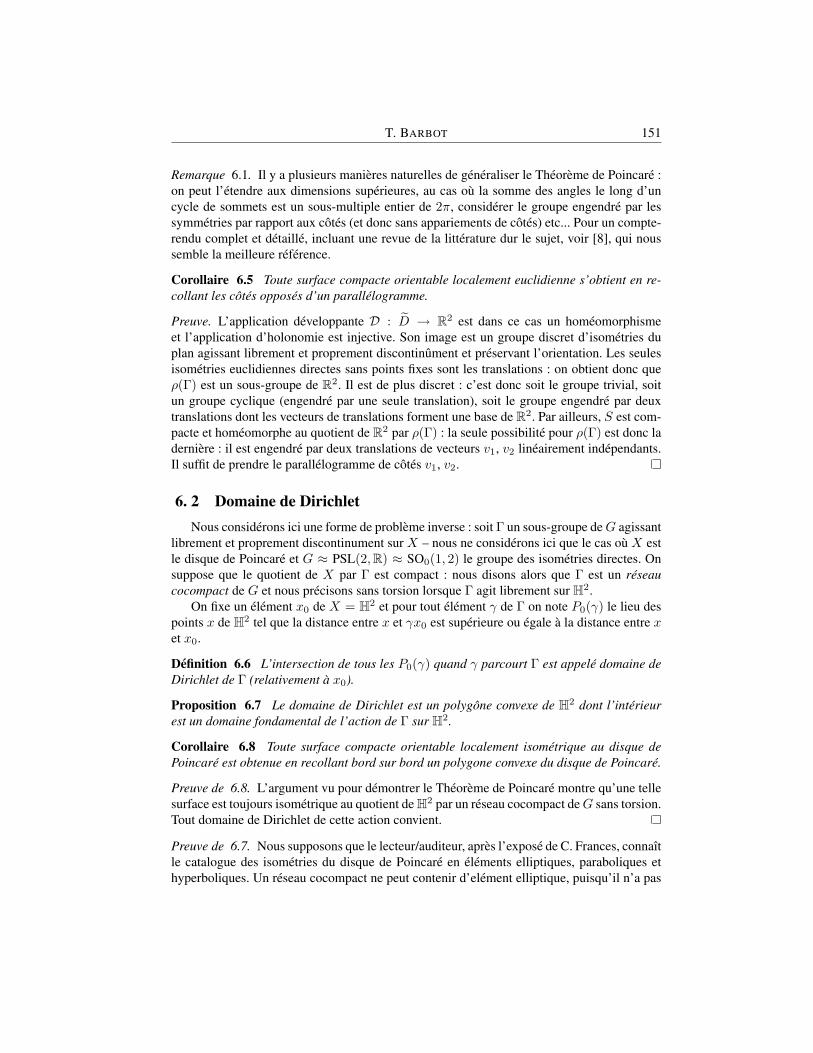
T. BARBOT 151
Remarque 6.1. Il y a plusieurs manieres naturelles de generaliser le Theoreme de Poincare :on peut l’etendre aux dimensions superieures, au cas ou la somme des angles le long d’uncycle de sommets est un sous-multiple entier de 2π, considerer le groupe engendre par lessymmetries par rapport aux cotes (et donc sans appariements de cotes) etc... Pour un compte-rendu complet et detaille, incluant une revue de la litterature dur le sujet, voir [8], qui noussemble la meilleure reference.
Corollaire 6.5 Toute surface compacte orientable localement euclidienne s’obtient en re-collant les cotes opposes d’un parallelogramme.
Preuve. L’application developpante D : D → R2 est dans ce cas un homeomorphismeet l’application d’holonomie est injective. Son image est un groupe discret d’isometries duplan agissant librement et proprement discontinument et preservant l’orientation. Les seulesisometries euclidiennes directes sans points fixes sont les translations : on obtient donc queρ(Γ) est un sous-groupe de R2. Il est de plus discret : c’est donc soit le groupe trivial, soitun groupe cyclique (engendre par une seule translation), soit le groupe engendre par deuxtranslations dont les vecteurs de translations forment une base de R2. Par ailleurs, S est com-pacte et homeomorphe au quotient de R2 par ρ(Γ) : la seule possibilite pour ρ(Γ) est donc laderniere : il est engendre par deux translations de vecteurs v1, v2 lineairement independants.Il suffit de prendre le parallelogramme de cotes v1, v2.
6. 2 Domaine de DirichletNous considerons ici une forme de probleme inverse : soit Γ un sous-groupe deG agissant
librement et proprement discontinument sur X – nous ne considerons ici que le cas ou X estle disque de Poincare et G ≈ PSL(2,R) ≈ SO0(1, 2) le groupe des isometries directes. Onsuppose que le quotient de X par Γ est compact : nous disons alors que Γ est un reseaucocompact de G et nous precisons sans torsion lorsque Γ agit librement sur H2.
On fixe un element x0 de X = H2 et pour tout element γ de Γ on note P0(γ) le lieu despoints x de H2 tel que la distance entre x et γx0 est superieure ou egale a la distance entre xet x0.
Definition 6.6 L’intersection de tous les P0(γ) quand γ parcourt Γ est appele domaine deDirichlet de Γ (relativement a x0).
Proposition 6.7 Le domaine de Dirichlet est un polygone convexe de H2 dont l’interieurest un domaine fondamental de l’action de Γ sur H2.
Corollaire 6.8 Toute surface compacte orientable localement isometrique au disque dePoincare est obtenue en recollant bord sur bord un polygone convexe du disque de Poincare.
Preuve de 6.8. L’argument vu pour demontrer le Theoreme de Poincare montre qu’une tellesurface est toujours isometrique au quotient de H2 par un reseau cocompact deG sans torsion.Tout domaine de Dirichlet de cette action convient.
Preuve de 6.7. Nous supposons que le lecteur/auditeur, apres l’expose de C. Frances, connaıtle catalogue des isometries du disque de Poincare en elements elliptiques, paraboliques ethyperboliques. Un reseau cocompact ne peut contenir d’element elliptique, puisqu’il n’a pas

152 GEOMETRIES ET DYNAMIQUES
de point fixe dans H2. On peut aussi voir qu’il ne peut contenir d’element parabolique :l’argument est un peu plus elabore, c’est le suivant : d’une part, par compacite de S = Γ\H2,il existe un reel positif ε tel que toute geodesique fermee de S est de longueur au moins ε.Par ailleurs, pour toute isometrie parabolique g, il existe un point x de H2 tel que la distanceentre x et gx est strictement inferieure a ε. Ces deux observations sont contradictoires.
Tous les elements de Γ sont donc hyperboliques : il sont chacun conjugue a une trans-formation de la forme z 7→ λz du demi-plan superieur H2. On peut en deduire, apres calcul,que chaque P0(γ) est un demi-plan, i.e. une composante connexe du complementaire d’unegeodesique de H2 (la mediatrice de (x0, γx0)). Le domaine de Dirichlet est donc une inter-section de demi-espaces : c’est un domaine convexe ferme de H2. Il est non-vide, puisqu’ilcontient x0. Nous le notons Ω et notons Ω son interieur : remarquez qu’on ne sait pas encoreque Ω est l’adherence de Ω – ni meme a priori que Ω est non-vide !
On remarque ensuite que pour tout R, il n’existe qu’un nombre fini d’elements γ de Γpour lesquels la boule BR de centre x0 et de rayon R rencontre la geodesique ∂P0(γ) : eneffet, si BR rencontre ∂P0(γ) en un point x, alors d(x0, γx0) ≤ d(x0, x) + d(x, γx0) =2d(x, x0) ≤ 2R. Donc, la boule B2R rencontre son image par γ ; comme l’action de Γ estproprement discontinue, nous avons demontre notre affirmation. Il s’ensuit que l’intersectionBR ∩ Ω est l’intersection entre BR et un polygone convexe non vide : l’intersection de tousles P0(γ) dont le bord rencontre BR. Ceci permet de montrer que Ω est bien l’adherence deΩ.
Nous voyons maintenant que l’union de tous les γΩ est H2 tout entier. En effet : soitx un point de H2. S’il n’est pas dans Ω, il existe un element γ de Γ tel que d(x, γx0) <d(x, x0). Posons x1 = γ−1x : nous avons d(x0, x1) < d(x0, x). Si x1 n’est pas dans Ω,en appliquant la meme procedure, on trouve un element x2 dans l’orbite de x pour lequeld(x0, x2) < d(x0, x1) < d(x0, x). De proche en proche, on construit une suite de points xndans la Γ-orbite de x, dont la distance a x0 est strictement decroissante. Si ce processus estsans fin, i.e. si aucun des xn n’est dans Ω, on obtient une suite infinie de points contenus dansla boule centree en x0 de rayon d(x, x0) : ceci contredit la proprete de l’action de Γ. Donc,un des iteres xn est dans Ω : notre assertion est demontree.
Nous sommes en mesure de demontrer que Ω est un domaine fondamental : il suffit dedemontrer que Ω ∩ γΩ est vide si γ 6= id. Soit x un point d’une telle intersection s’il enexiste : alors, pour tout γ′, γ′′, on a d(x, x0) ≤ d(x, γ′x0) et d(γ−1x, x0) ≤ d(γ−1x, γ′′x0).En prenant γ′ = γ et γ′′ = γ−1, on obtient d(x, x0) = d(x, γx0), ce qui montre que xappartient a la frontiere de Ω et non pas a son interieur Ω. Contradiction.
Nous affirmons maintenant que Ω est compact. Soit pn une suite d’elements de Ω : commela surface quotient S est compacte, il existe une suite d’elements γn de Γ tels que γnpnconvergent vers un point p de H2. Comme Ω est un domaine fondamental, quitte a composerles γn par un element de Γ, on peut supposer que p appartient a Ω. Si p appartient a Ω, lesγnpn appartiennent eux aussi a Ω, ce qui n’est possible que si tous les γn sont triviaux : lespn convergent vers p.
Il reste le cas ou Si p appartient a la frontiere ∂Ω. Soit U une boule compacte centree enp : tous les γnΩ rencontrent U ; si γnΩ 6= Ω, il existe un point q dans U tel que d(γnx0, q)−d(x0, q) < 0, alors que d(γnx0, p) − d(x0, p) ≥ 0 : on en deduit que ∂P0(γn) rencontreU ; or, nous avons vu auparavant que ceci signifie que les γn sont en nombre fini. Donc, laencore, les pn convergent dans H2 et donc dans le ferme Ω.

T. BARBOT 153
Etant compact, Ω est contenu dans une boule BR. C’est donc un polygone convexe.
7 Groupes de SchottkyLe theoreme de Poincare s’etend au cas non-compact : de maniere plus general, au
lieu de se restreindre aux convexes compacts de H2, on peut considerer tout domaine Pd’interieur non vide intersection de demi-espaces de H2, etant convenu qu’un demi-espaceest (l’adherence d’) une composante connexe du complementaire d’une geodesique complete.
De maniere plus precise : soit P1, ... , P2k un nombre fini de tels demi-espaces tels quesi i 6= j, alors (H2 \ Pi) ∩ (H2 \ Pj) = ∅. On note P l’intersection de tous les Pi : c’estun domaine convexe qui n’est surement pas compact. On choisit un appariement σ, i.e. uneinvolution de 1, ...2k dans lui-meme : il existe alors toujours une isometrie envoyant ledemi-espace (H2 \ Pi) sur l’interieur de Pσ(i). Il en existe en fait plusieurs, qui differentles unes des autres par des transformations hyperboliques le long de ∂Pi. Nous choisissonsd’entre elles pour chaque i, que nous notons γσi , de sorte que γσσ(i) soit l’inverse de γσi . Onrecolle P le long de ces bords geodesiques selon ces γσi : on obtient une surface S localementisometrique au disque de Poincare ; c’est meme plus facile de le verifier ici puisqu’il n’y a pasde sommets. On peut reproduire les constructions vues precedemment : construire un groupeabstrait Γ agissant sur une surface abstraite S obtenues en recollant des copies de P , ainsiqu’une application developpante D : S → H2 et une representation d’holonomie ρ : Γ →PSL(2,R). Dans ce cas, comme il n’y a pas de sommets, il n’y a pas de cycles de sommets !Les seules relations intervenant dans la definition de Γ sont les relations (a, σ(a)) ≈ (∅), quisont par ailleurs bien sur necessaires pour que Γ soit un groupe. En d’autres termes, Γ estun groupe dit libre puisqu’il n’admet pas d’autres relations que celles admises par tous lesgroupes. Ce que nous avons dit reste assez flou, precisons-le :
Definition 7.1 Un element de Γ (dit aussi mot de l’alphabet A = 1, ...2k) est reduit s’ilne contient pas deux termes successifs de la forme (a, σ(a)).
Il doit etre clair que tout element de Γ est equivalent a un mot reduit (car, eliminer uneoccurence (a, σ(a)) reduit la longueur du mot) et donc, que tout element de Γ est representepar un mot reduit. Il est moins clair que deux mots reduits ne sont equivalents que s’ils sontegaux, mais ce sera un des corollaires du lemme suivant bien connu :
Lemme 7.2 (lemme du ping-pong) L’image par ρ d’un mot reduit (i1, ...., iq) envoie Pdans Pσ(i1).
Preuve. Pour montrer ce lemme, il suffit de montrer le fait suivant un peu plus precis :L’image par ρ d’un mot reduit (i1, ...., iq) envoie H2 \ Piq dans Pσ(i1).Cela se demontre par recurrence sur la longueur du mot.
Corollaire 7.3 L’application ρ est injective.
Corollaire 7.4 Deux mots reduits ne representent le meme element de Γ que s’ils sontegaux. En particulier, un mot reduit ne represente l’element trivial de Γ que s’il est vide.

154 GEOMETRIES ET DYNAMIQUES
Nous laissons au lecteur le soin de s’assurer que l’action de ρ(Γ) sur H2 est libre etproprement discontinue, le quotient etant une surface S localement isometrique au disque dePoincare et complete. Les groupes ρ(Γ) obtenus par ce procede sont dits groupes de Schottky.
Mais il y a une difference de taille avec le cas ou P est un polygone compact : La surfacerecollee S n’est pas necessairement complete ! En d’autres termes, il se peut que S et S nesoient pas isometriques, que l’application developpanteD ne soit pas surjective... Il est quandmeme toujours vrai que D est injective et que son image est un domaine convexe de H2... Lemieux est sans doute d’etudier de soi-meme ces situations. Pour les impatients, voir [8].
Indiquons quand meme un cas un peu plus agreable : on considere la figure dans le com-pactifie conforme du disque de Poincare, H2
: si les adherences dans H2des H2 \ Pi sont
deux-a-deux disjointes, la surface S est complete ; en d’autres termes, P est un domainefondamental de ρ(Γ). Il arrive que certains auteurs reservent la terminologie « groupe deSchottky » a ce cas particulier.
T. BARBOT 155
TROISIEME SCEANCE : TROUS NOIRS BTZ
Nous indiquons ici quelques excellents textes : l’incontournable [11], [13] traitant demaniere detaillee a souhait l’espace-temps de Kerr, ainsi que le precieux [7], qui a l’extremeavantage d’etre en libre service. Nous supposons connues les notions de metrique lorent-zienne, courbe de type temps, espace, lumiere ou causale, ainsi que futur (ou passe) causalou temporel d’une region.
8 L’espace de SchwarzschildIl est remarquable que des 1916, alors qu’Einstein ne publia la forme exacte de son
equation qu’en 1915, K. Schwarzschild, hospitalise pour maladie (fatale) sur le front russe,trouva une famille a un parametre de solutions exactes de l’equation d’Einstein dans levide, avec constante cosmologique nulle. Cette famille est assez deconcertante (du moinsa l’epoque), et se revela par la suite des plus pertinentes pour d’ecrire le voisinage d’un corpsceleste, typiquement, une etoile et amenant a la notion meme de trou noir. Elles ne dependentque d’un seul parametre, qui s’interprete aisement comme la masse d’un corps celeste isole.
Du reste, un theoreme fameux (theoreme de Birkhoff) enonce que ces solutions sont lesseules a symetrie spherique. Une formulation exacte et precise de ce theoreme demanderaidavantage de commentaires, mais ce n’est pas notre sujet.
Ces espaces temps, dans les coordonnees dites (justement) de Schwarzschild, ont unemetrique qui s’exprime sous la forme3 :
ds2 = −(1− 2Mr
)dt2 +dr2
1− 2M/r+ r2ds2
0
Dans cette expression, ds20 = dθ2 + sin2 θdφ2 designe la metrique de la sphere ronde
S2. On doit aussi comprendre que R4 est pense muni de coordonnees (x, y, z, t), que r vaut√x2 + y2 + z2 et (θ, φ) sont les coordonnees spheriques de (xr ,
yr ,
zr ) ∈ S2.
On remarque que ceci n’est pas une metrique sur tout R4, mais sur R4 prive des lieuxsinguliers r = 0 et r = 2M . De fait, il est preconise de ne penser cette expression que commeetant valable sur une carte particuliere d’un espace-temps MKS plus vaste, diffeomorphe auproduit de R2 par la sphere S2, sur laquelle la solution meme de Schwarzschid s’etend en unemetrique lorentzienne – les facteurs S2 etant toujours des orbites d’une action de SO(3). Onparle alors de systeme de coordonnees de Kruskal-Szekeres (bien qu’il ne s’agisse pas d’unsysteme de coordonnees sur R4 ! ). Ce nouvel espace-temps est alors maximal : il ne peut etreplonge isometriquement dans un autre espace-temps plus grand. Donnons l’expression de sametrique : on munit R2 de coordonnees (u, v), on note U l’ouvert v2 − u2 < 1, on definitune fonction r = r(u, v) par la relation :
(r/2M − 1)er/2M = u2 − v2
3Apres normalisation affectant a la vitesse de la lumiere c et a la constante gravitationnelleG la valeur commune1.

156 GEOMETRIES ET DYNAMIQUES
On peut alors definir sur U × S2 la metrique lorentzienne suivante :
ds2KS = (32M3/r)e−r/2M (−dv2 + du2) + r2ds2
0
U×S2 muni de cette metrique ds2KS est precisement l’espaceMKS de Kruskal-Szerekes.
Notez que l’affectation du nom r a la fonction ci-dessus n’est pas arbitraire : la zone r >2M,u > 0 (respectivement 0 < r < 2M,v > 0) de MKS est isometrique au domainer > 2M (respectivement 0 < r < 2M) de l’espace de Schwarzschild. Il apparaitainsi que r = 2M n’etait pas une reelle singularite, puisqu’il suffit de se placer dans lebon systeme de coordonnees pour faire disparaitre cette singularite. Par contre, la singulariter = 0 persiste.
Les zones B+ = u2 < v2, v > 0 et B− = u2 < v2, v < 0 sont remarquables :aucune courbe causale orientee vers le futur (i.e. sur laquelle v est une application croissante)et issue d’un point de B+ ne peut s’echapper de B+ et, de maniere analogue, aucune courbecausale orientee vers le futur ne peut penetrer dans B−. On dit que B+ est un trou noir, B−
un trou blanc et MKS lui-meme est qualifie de « trou de ver » (wormhole en anglais). Toutlecteur (meme occasionnel) de science-fiction comprendra les raisons de ces termes.
Ces notions semblent naturelles, mais insistons sur le presuppose sur lequel elles re-posent : on part du principe que l’observateur λ est dans la zone u2 − v2 > 0 et donc, lazone B+ lui semble effectivement mysterieuse, puisqu’aucun signal emanant de cette regionne peut lui parvenir. De plus, la singularite u2 = v2, v > 0, qu’un voyageur intrepide etinsouciant pourrait atteindre en un temps (propre) fini, lui est invisible (cela, du reste, quandbien meme lui prendrait la fantaisie de penetrer dans B+) – remarquons quand meme qu’ilobserve partout les signaux emis par la singularite r = 0, v < 0, qu’il est tentant de quali-fier de « Big Bang ». Mais au nom de quel principe faut-il privilegier la zone u2 − v2 > 0comme etant le lieu naturel d’un citoyen normal ?
On peut instituer cette regle de bonnes mœurs de la maniere suivante : il existe une com-pactification conforme naturelle de MKS , obtenues en adjoignant un bord, dit bord de Pen-rose. Nous n’avons pas le temps ici de developper cette notion de compactification conforme– nous preferons le faire ulterieurement dans le cadre des trous noirs BTZ. Disons au moinsque la partie « future » de cette compactification est l’ensemble des rayons geodesiquesorientes vers le futur complets, quotiente par une certaine relation d’equivalence. De manieremoins elaboree, mais plus precise et repondant aussi bien a la question que nous venons desoulever, on peut caracteriser MKS \B+ comme etant le lieu des points a partir desquels onpeut envisager effectuer un trajet causal de temps propre infini (le cas limite u2 = v2, v ≥ 0demandant une certaine adresse, sans aucun droit a l’erreur et necessitant de voyager a la vi-tesse de la lumiere).Remarque 8.1. L’espace de Schwarzschild admet une generalisation naturelle : l’espace deReissner-Nordstrom, qui est aussi une solution a symetrie spherique de l’equation d’Einstein,mais pas dans le vide ; en presence d’un champ electromagetique. Son expression est :
ds2 = −∆dt2 + ∆−1dr2 + r2ds20
ou :
∆ = 1− 2Mr
+p2 + q2
r2

T. BARBOT 157
M s’interprete toujours comme etant la masse du corps celeste, p sa charge electriquetotale et q sa charge magnetique totale.
On peut dans ce cas plonger cette variete lorentzienne dans un espace temps maximalMmaxRS , mais de description beaucoup plus delicate que celle de MKS ! De maniere expediti-
ve, decrivons succintement les proprietes causales de MmaxRS : on peut d’abord etendre l’es-
pace de Reissner-Nordstrom (primitif) en un espace diffeomorphe a R2×S2, que nous appel-lerons « bloc RN ». Si la force electro-magnetique est trop importante, i.e. M < p2 + q2, cebloc admet ce qu’on appelle une singularite nue, qui, pour parler succintement (et de manierefloue) peut etre atteinte en un temps fini, puis etre quittee. Les physiciens excluent ce casde figure et le proscrivent comme etant physiquement irrealiste : c’est ce qu’on appelle laCensure Cosmique (cachez cette singularite que je ne saurai voir).
Par contre, si M > p2 + q2, le bloc admet des proprietes similaires a celles de MKS : ilexiste un trou noir B+ tel que B+ est invisible pour tout observateur decrivant dans ce blocune trajectoire causale de temps propre infini. Mais une premiere difference essentielle estque meme apres avoir penetre dans B+, un voyageur a de tres bonnes chances de pouvoircontinuer son parcours en un temps propre infini ! Cependant, il ne pourra le faire en restantdans le bloc, il rentrera plutot dans une autre copie de ce bloc, dans sa partie B− du reste.Ainsi, Mmax
RS s’obtient en empilant une infinite de blocs, se connectant les uns aux autresselon leurs regions B±.
Une autre difference essentielle est que si on considere tout le bord conforme de MKS ,il n’y a plus de region invisible. En d’autres termes, tout point de MKS est visible depuis lebord conforme. La notion de trou noir est ainsi relative a chaque bloc RN ; le point de vue aadopter est que chaque observateur est confine au bord conforme d’un de ses blocs et il existealors bien une partie du bloc RN qui lui reste opaque.
Il y a aussi une autre generalisation de la metrique de Schwarzschild, aux proprietescausales fascinantes : l’espace de Kerr, pouvant etre interprete comme cree par un corpsceleste a symetrie spherique, mais anime d’un mouvement de rotation. Le (tres bon) livre[13] lui est tout entier consacre.
Sa metrique, dans une carte particuliere d’un ouvert correspondant a l’exterieur d’un voi-sinage du corps celeste, s’exprime sous la forme suivante :
−(1− 2Mr
ρ2)dt2 +
ρ2
∆dr2 − sin2(θ)
4Mra
ρ2dφdt+ ρ2dθ2
+(r2 + a2 + sin2(θ)2Mra
ρ2) sin2(θ)dφ2
Avec :– ∆ = r2 − 2Mr + a2 et ρ2 = r2 + a2 cos2(θ),– M une quantite positive representant la masse,– a une quantite representant le moment angulaire par unite de masse.Notons que quand a vaut 0, on retrouve l’expression de Schwarzschild. Les deux derniers
termes definissent une metrique sur la sphere affectees des coordonnees θ, φ, qui n’est plusun multiple de la metrique usuelle de la fibre. Notons aussi que la translation dans le temps test toujours une isometrie, mais il n’y a pas d’hypersurface orthogonale a ces trajectoires detemps (on dit que Kerr n’est pas statique, contrairement a Schwarzschild).

158 GEOMETRIES ET DYNAMIQUES
L’espace de Kerr, tel que decrit ci-dessus, admet lui aussi une extension maximale, obte-nue en recollant des parties particulieres, de maniere analogue a la construction de l’espace deReissner-Nordstrom maximal. La description de la structure causale sur cet espace maximalest delicate, indiquons brievement ici que la encore, l’espace de Kerr maximal se decomposeen blocs successifs, le suivant dans le futur du precedent et qu’on ne peut atteindre le blocsuivant qu’en traversant l’horizon d’un trou noir et en emergeant dans un « trou blanc ».
Une des proprietes remarquables et surprenantes de (l’extension maximale de) l’espacede Kerr est le fait que son flot geodesique est totalement integrable, au sens ou il existesuffisamment de fonctions invariantes par le flot geodesique pour distinguer toutes ses orbites– les symetries de l’espace de Kerr (avec le Theoreme de Noether) fournissent plusieurs deces fonctions invariantes, mais elles ne suffisent pas, il y a un autre invariant, dit invariant deCarter, d’origine un peu mysterieuse et qui complete la famille de fonctions invariantes.
9 L’espace anti-de Sitter
9. 1 DefinitionsL’espace anti-de Sitter de dimension n, note AdSn, est la variete lorentzienne definie de
la maniere suivante : on note R2,n−1 l’espace vectoriel de dimension n+ 1, muni de la formequadratique :
Q = −u2 − v2 + x21 + ...+ x2
n−1
L’espace anti-de Sitter AdSn est le lieu ou cette forme quadratique vaut −1, equippe dela metrique lorentzienne obtenue en restreignantQ aux espaces tangents. Le groupe d’isome-tries lorentziennes de AdSn contient manifestement SO0(2, n − 1), la composante connexede l’identite de SO(2, n − 1) et il n’est pas difficile de montrer qu’il s’agit la de toutes lesisometries preservant l’orientation de AdSn ainsi que son orientation chronologique. Nousconsidererons aussi le modele de Klein de l’espace anti-de Sitter : il s’agit de la projectionradiale, notee de ADSn de AdSn dans l’espace projectif RPn+1 de Rn+1. Observons queAdSn est un revetement double de ADSn.
Nous ne considererons ici que le cas n = 3, i.e. l’espace anti-de Sitter AdS3. Remarquonstout d’abord que l’oppose de l’application determinant (notee −det) sur M(2,R), espacevectoriel des matrices 2×2, est justement une forme quadratique non degeneree de signature(2, 2). Ainsi, AdS3 s’identifie a SL(2,R) ⊂ M(2,R), equipe de la restriction de −det. Deplus, l’action de SL(2,R) × SL(2,R) sur SL(2,R) par (a, b).g = agb−1 est une actionisometrique pour la metrique lorentzienne induite par −det. Ceci montre que O(2, 2), legroupe des isometries deAdS3, contient (quasiment) un sous-groupe isomorphe a SL(2,R)×SL(2,R).
Ceci n’est pas tres correct puisque l’element (−Id,−Id) de SL(2,R) × SL(2,R) agittrivialement sur SL(2,R). On considere donc plutot l’action sur le modele de Klein ADS3,dontAdS3 est un revetement double ; il est alors correct de dire que PSL(2,R)×PSL(2,R)est isomorphe a la composante neutre du groupe des isometries de ADS3.
Cette simple remarque permet de trouver plethore de quotients compacts de AdS3 : pren-dre n’importe quel sous-groupe discret Γ cocompact de PSL(2,R) ≈ SO0(1, 2) (en par-

T. BARBOT 159
tant par exemple d’un polygone dans le disque de Poincare) ; l’action de Γ sur PSL(2,R)par translations a gauche est alors une action cocompacte sur ADS3 ≈ PSL(2,R) parisometries.
9. 2 Quelques proprietes geometriques
Le bord conforme
Nous notons ∂ADS3 la frontiere de ADS3 dans RP 3 : nous l’appelons bord conformede ADS3. L’union ADS3 ∪ ∂ADS3 est notee ADS3, nous l’appelons compactifie conformede ADS3. C’est bien sur l’adherence de ADS3 dans RP 3. Par revetement double, on peutdefinir le bord conforme ∂AdS3 et le compactifie conforme AdS3.
L’hyperboloıde
L’ouvert ADS3 de RP 3, intersecte avec une carte affine≈ R3 bien choisie est le domainesimplement connexe borde par une hyperboloıde a une nappe ; nous noterons H ce domaineouvert. Pour reobtenir ADS3 tout entier a partir de ce domaine, il suffit de lui adjoindre undisque contenu dans le plan projectif bordant la carte affine dans RP 3. Du reste, ce disque,muni de la restriction de la metrique lorentzienne ambiante, est isometrique au disque dePoincare, on peut aussi dire que c’est une version du modele de Klein du disque de Poincare.
Geodesiques
Les geodesiques de AdS3 sont les intersections de cette nappe avec les 2-plans de R2,2 ;dans ADS3, ce sont donc les intersections entre ADS3 et les droites projectives de RP 3. Lesdroites qui ne rencontrent pas ∂ADS3, i.e. contenues dans ADS3, sont des geodesiques detype temps ; celles qui rencontrent ∂ADS3 en deux points distincts sont, quand on prend leurintersection avec ADS3, des geodesiques de type espace ; enfin, celles qui sont tangentes enun point de ∂ADS3 sont de type lumiere.
Isometries, champs de Killing
Nous entendrons ici par groupe des isometries de ADS3 ≈ PSL(2,R) le sous-grouped’indice fini PSL(2,R)× PSL(2,R). Comme nous nous interesserons surtout aux champsde Killing, cette restriction a un sous-groupe d’indice fini n’a aucune incidence. Un champde Killing est un sous-groupe a un parametre de ce groupe, c’est donc en fait la donnee dedeux sous-groupes a un parametre de PSL(2,R).
Une classe de conjugaison dans Isom(ADS3) correspond donc a la donnee de deuxclasses de conjugaison d’elements de PSL(2,R), or, ces dernieres classes sont bien com-prises : elles sont elliptique, parabolique ou hyperbolique (cf. cours C. Frances). Notonsque deux elements paraboliques sont toujours soit conjugues entre eux soit l’un conjuguea l’inverse de l’autre. Par contre, les sous-groupes elliptiques sont distingues entre eux parun nombre reel, indiquant a quelle vitesse les cercles concentriques sont parcourues par lesorbites. En d’autres termes, le groupe elliptique de parametre a est :

160 GEOMETRIES ET DYNAMIQUES
t 7→(
cos(aθ) sin(aθ)− sin(aθ) cos(aθ)
)Le groupe hyperbolique de parametre r est :
t 7→(
exp(rt) 00 exp(−rt)
)
9. 3 Revetement universel
L’espace anti-de Sitter n’est pas simplement connexe : nous noterons AdS3 son reve-tement universel. En fait, comme toute matrice de rang 2 s’ecrit sous la forme KT , ou Kest une rotation (element de SO(2)) et T une matrice triangulaire superieure a coefficientsdiagonaux positifs, on obtient que AdS3 est diffeomorphe au produit du cercle par R2. Songroupe fondamental est monogene, engendre par un element que nous noterons δ et AdS3
s’identifie au quotient de AdS3 par l’action du groupe engendre par δ.Le revetement universel peut etre decrit de la maniere suivante : on empile une infinite de
copiesHi (i ∈ Z) du domaineH decrit ci-dessus, en joignant deux tels domaines successifsHi, Hi+1 par une copie du modele de Klein du disque de Poincare. L’application δ envoiechaqueHi sur son voisinHi+1.
9. 4 Causalite.
Le futur (resp. passe) d’un point x0 dans une variete lorentzienne est le lieu des pointspouvant etre atteint par une courbe de type temps issue de x0 et orientee vers le futur (respec-tivement passe). Si on autorise en outre les courbes causales, on obtient le futur dit causal.cette notion dans AdS3 ou ADS3 est triviale : tout point est dans le futur et dans le passede tout point. Par contre, cette notion n’est pas triviale dans le revetement universel AdS3.On peut la decrire geometriquement de la maniere suivante : soit x0 un point de AdS3, seprojettant sur un point x0 de AdS3 et [x0] de ADS3. Notons P0 l’orthogonal de x0 pour laforme quadratique ambiante de R2,2. Le complementaire de la projection de P0 dans RP 3 estune carte affine, de coordonnees (x, y, z), ou les points appartenant a ADS3, i.e. a H, sontceux satisfaisant :
x2 + y2 < 1 + z2
On peut choisir ces coordonnees de sorte que [x0] soit de coordonnees (0, 0, 0). Rappelonsque AdS3 est obtenu en empilant des copiesHi deH (et en prenant les parties communes deleurs adherences) ; on peut convenir que H0 = H et que chaque Hi+1 (resp. Hi−1 soit dansle futur (resp. passe) deHi. Le futur (resp. passe) de [x0] consiste alors en l’union de :
– l’adherence de chaqueHi, avec i > 0 (resp. i < 0),– l’ensemble des points deH verifiant : z2 < x2 + y2 et z > 0 (resp. z < 0).

T. BARBOT 161
10 Trous noirs BTZ
L’etude des quotients compacts de AdS3, aussi interessante quelle soit ([14]) n’est pasnotre veritable preoccupation dans ce cours. Nous gravitons plutot autour de l’analogue dutheoreme de Birkhoff en dimension 2 + 1, en cherchant quelle est la forme raisonnable d’es-paces temps representant des corps celestes isoles, en rotation sur eux memes ou non. Unereference adaptee pour completer cette section est [1] (a lire avec precaution, mais ce textereste un des meilleurs, et s’inscrit dans un point de vue proche de ce qui est developpe ici).
Tout d’abord, comme nous l’avons evoque precedemment, une variete lorentzienneM dedimension 2 + 1 satisfaisant l’equation d’Einstein (dans le vide, de constante cosmologiqueΛ) est necessairement a courbure sectionnelle constante K, de signe egal a celui de Λ. Cecisignifie que la metrique lorentzienne est celle provenant d’une (G,X)-structure sur M , ouX est la variete lorentzienne modele de courbure constante K et G le groupe des isometriesde X (preservant l’orientation, ainsi qu’une orientation chronologique de X). La condition« symetrie spherique », apparaissant dans le theoreme de Birkhoff (valable en dimension3 + 1) signifie dans ce cas l’existence d’un groupe d’isometries isomorphe a SO(2), dontles orbites sont des courbes de dimension 1 de type espace. Un tel champ de Killing estle tire en arriere par (la differentielle de) l’application developpante d’un champ de KillingY sur X , mais qui n’est pas necessairement periodique. En fait, le fait que les orbites surla (G,X)-variete soient toutes periodiques, de meme periode T , se traduit par la conditionsuivante sur Y : le temps T du flot engendre par Y doit appartenir au groupe d’holonomie. Deplus, le groupe d’holonomie doit preserver Y , ce qui signifie que tous les elements du grouped’holonomie doivent commuter avec chaque element du groupe a un parametre d’isometriesengendre par Y . Enfin, le fait que les orbites du champ de Killing sur M soient spatialesequivaut a requerir que l’application developpante prend ses valeurs dans l’ouvert de X oules orbites de Y sont de type espace.
Ces conditions sont satisfaites par plusieurs exemples de (G,X)-varietes. Plutot que dis-cuter en general toutes les situations possibles, nous preferons ajouter une hypothese supple-mentaire, naturelle si on souhaite que M joue le role de la geometrie d’un espace-tempscree par un corps celeste dans son voisinage4 : on demande a ce que M soit diffeomorphe aS1 × R2.
Dans ce cas, le groupe d’holonomie est en definitive engendre par l’element γ = Y T deG. On n’oubliera pas dans la suite que γ est le temps T d’un champ de Killing Y .
Nous n’allons considerer ici que le cas ou la constante cosmologique est negative, i.e.celui ou l’espace-temps est une (G,X)-variete, avec X = ADS3 ≈ PSL(2,R) et G =PSL(2,R)× PSL(2,R). C’est du reste un excellent exercise que de reproduire cette etudedans le cas ou X est l’espace de Minkowski, ou encore celui ou il est l’espace de Sitter (pourceux qui le connaissent). Alors, γ est une paire d’elements (γ1, γ2) de PSL(2,R). Notonsque conjuguer γ dans PSL(2,R)×PSL(2,R) par un element h revient a composer l’appli-cation developpante par h : ceci ne modifie pas la (G,X)-structure. Nous n’avons donc qu’unnombre fini de cas a considerer, repertories dans [2] et [1] – mais avec une nomenclature des
4Nous aurions pu d’entree introduire cette hypothese, court-circuitant toute la discussion precedente, mais j’aijuge utile de faire une mise au point utile pour apprecier a sa juste valeur l’argumentation faite dans [2] pour jus-tifier l’affirmation selon laquelle les metriques BTZ sont les solutions stationnaires a symetrie axiale de l’equationd’Einstein.

162 GEOMETRIES ET DYNAMIQUES
plus inelegantes a nos yeux. Tous les cas sont etudies dans [2], mais il s’agit la encore d’unbon exercice qu’il est utile de pratiquer soi-meme.
Dans chacun de ces cas, on determine la region de ADS3 ou le champ de Killing Y estde type espace, on le note Ω(γ). Il s’avere que dans tous les cas, l’action du groupe engendrepar γ sur Ω(γ) est libre et proprement discontinue (mais notez que pour certains γ, Ω(γ) estvide !). Le quotient M(γ) de Ω(γ) par cette action est alors une variete localement anti-deSitter. De plus et cela n’est pas veritablement une tautologie, cette variete lorentzienne estcausale, au sens ou elle ne contient aucune courbe causale periodique.
En definitive, seul merite un interet soutenu le cas ou γ1 et γ2 sont tous les deux hyperbo-liques (il y a aussi le cas, dit extreme, ou γ1 et γ2 sont deux elements paraboliques conjugues,mais que nous mettons lui aussi de cote dans ces notes). La variete M(γ) est dans ce casappelee Trou noir BTZ (selon les initiales des auteurs de la premiere version de [2]). Notonsque cette terminologie est assez trompeuse : M(γ) tout entier n’est pas un trou noir, maiscontient une zone meritant d’etre interpretee comme un trou noir, tant elle presente des simi-litudes frappantes avec la zone B+ d’un espace de Schwarzschild ou de Kerr. C’est ce quenous souhaitons mettre en avant dans la suite.
Notons d’abord que M(γ), a isometrie pres, ne depend dans ce cas que des classes deconjugaison de γ1 et γ2. Nous definissons deux nombres reels 0 ≤ r− < r+ de sorte que :
γ1 =(eπ(r+−r−) 0
0 e−π(r+−r−)
), γ2 =
(eπ(r++r−) 0
0 e−π(r++r−)
)Le sous groupe a un parametre correspondant agit sur PSL(2,R) de la maniere suivante :
Y t(g) =(etπ(r+−r−) 0
0 e−tπ(r+−r−)
)(a bc d
)(e−tπ(r++r−) 0
0 etπ(r++r−)
)En derivant par rapport a t en t = 0, puis en prenant −det, on obtient que la norme de Y (g)est du signe de (en tenant compte de ad− bc = 1) :
(r2+ − r2
−)bc+ r2−
Donc, Ω(γ) est dans ce cas le lieu ou bc est strictement inferieur a r2−/(r
2+ − r2
−).
10. 1 Le cas statique r− = 0 :Ω(γ) est alors la zone bc < 0. Nous laissons au lecteur le soin de verifier qu’elle est conte-
nue dans une carte affine (par exemple, celle qui contient toutes les matrices non symetriques)et que si cette carte affine est bien choisie, l’ouvert Ω(γ), decrit dans la figure 1, est l’ouvertcompris entre deux hyperplans paralleles, chacun tangent a l’hyperboloide en des points x+,x−. Ces hyperplans sont b = 0 et c = 0 ; ils se prolongent en s’intersectant en unedroite dans le plan projectif a l’infini correspondant aux matrices diagonales, cette droite estla droite des zeros de Y (des points fixes de γ) (dans la figure, nous avons dessine deux tellesdroites a l’infini pour des besoins de perspective, mais ces deux segments doivent etre pensesconfondus. La figure devient correcte si on l’interprete comme etant le domaine Ω(γ) tronque
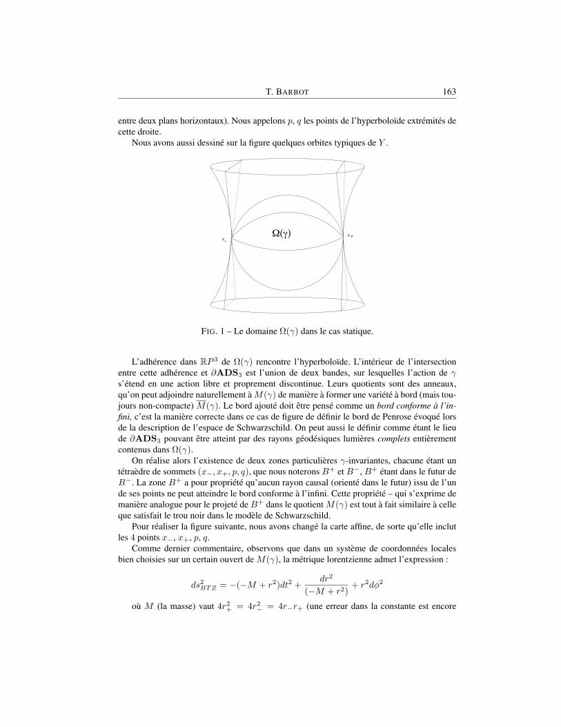
T. BARBOT 163
entre deux plans horizontaux). Nous appelons p, q les points de l’hyperboloıde extremites decette droite.
Nous avons aussi dessine sur la figure quelques orbites typiques de Y .
!(")x
x!
+
FIG. 1 – Le domaine Ω(γ) dans le cas statique.
L’adherence dans RP 3 de Ω(γ) rencontre l’hyperboloıde. L’interieur de l’intersectionentre cette adherence et ∂ADS3 est l’union de deux bandes, sur lesquelles l’action de γs’etend en une action libre et proprement discontinue. Leurs quotients sont des anneaux,qu’on peut adjoindre naturellement aM(γ) de maniere a former une variete a bord (mais tou-jours non-compacte) M(γ). Le bord ajoute doit etre pense comme un bord conforme a l’in-fini, c’est la maniere correcte dans ce cas de figure de definir le bord de Penrose evoque lorsde la description de l’espace de Schwarzschild. On peut aussi le definir comme etant le lieude ∂ADS3 pouvant etre atteint par des rayons geodesiques lumieres complets entierementcontenus dans Ω(γ).
On realise alors l’existence de deux zones particulieres γ-invariantes, chacune etant untetraedre de sommets (x−, x+, p, q), que nous noterons B+ et B−, B+ etant dans le futur deB−. La zone B+ a pour propriete qu’aucun rayon causal (oriente dans le futur) issu de l’unde ses points ne peut atteindre le bord conforme a l’infini. Cette propriete – qui s’exprime demaniere analogue pour le projete de B+ dans le quotient M(γ) est tout a fait similaire a celleque satisfait le trou noir dans le modele de Schwarzschild.
Pour realiser la figure suivante, nous avons change la carte affine, de sorte qu’elle inclutles 4 points x−, x+, p, q.
Comme dernier commentaire, observons que dans un systeme de coordonnees localesbien choisies sur un certain ouvert de M(γ), la metrique lorentzienne admet l’expression :
ds2BTZ = −(−M + r2)dt2 +
dr2
(−M + r2)+ r2dφ2
ou M (la masse) vaut 4r2+ = 4r2
− = 4r−r+ (une erreur dans la constante est encore

164 GEOMETRIES ET DYNAMIQUES
p
q
x
x+
!
B+
FIG. 2 – Le trou noir avant passage au quotient.
possible dans cette version preliminaire du texte). La convention implicite « φ definie modulo2π », i.e. φ = 0 identifie a φ = 2π, code le passage au quotient en identifiant selon γ.
10. 2 Le cas non-statique r− > 0 :Ce cas est alors similaire a l’espace de Kerr ! Notons que l’ouvert Ω dans le cas statique
ne depend pas de la valeur de r+, nous l’appelons ici sobrement Ω0.Une analyse automatique montre que Ω(γ) n’est plus contenu dans un seul ouvert affine
du type H. C’est en fait l’intersection dans RP 3 entre ADS3 et l’interieur d’un autre hy-perboloide (projectif) tangent a ∂ADS3 en les points x± et contenant les droites projectives(p, x±) et (q, x±) (voir figure 3).
La figure globale correcte est la suivante :AppelonsH0 l’ouvert affine contenant Ω0 decrit ci-dessus, mais nous le pensons mainte-
nant dans AdS3. Encore une fois, ce dernier est obtenu en empilant des copiesHi successivesdeH0 et, dans chacune de ces copies, il existe un exemplaire Ω(γ)i de Ω(γ) : ces exemplairess’ajoutent les uns aux autres pour former un ouvert5 Ω(γ) de AdS3. Le quotient de cet ou-vert par le releve de γ qui preserve chaque Ω(γ)i est une variete lorentzienne, a la structurecausale de laquelle on peut appliquer au mot pres notre description de l’espace de Reissner-Nordstrom maximal (et donc aussi celle de l’espace de Kerr maximal).
Enfin, on peut trouver dans certaines coordonnees locales l’expression suivante de lametrique BTZ, assez semblable a celle de Kerr ou celle de Reissner-Nordstrom :
dsBTZ = −(−M + r2 +J2
4r2)dt2 +
dr2
−M + r2 + J2/4r2+ r2(dφ− J
2r2dt)2
5Nous trichons un peu, il faut ajouter des parties communes dans les disques de Poincare de jonction, mais laformulation correcte nous semble aisee a trouver soi-meme.

T. BARBOT 165
x+x!
FIG. 3 – Le domaine Ω(γ).
avec M = r2+ + r2
− s’interpretant comme la masse, et J = 2r−r+ comme un momentangulaire. Les inegalites suivantes sont satisfaites :
M > 0, | J |≤M .
Bibliographie[1] S. Aminneborg, I. Bengtsson, S. Holst, A spinning anti-de Sitter wormhole, Class.
Quant. Grav., 16 (1999), 363–382, gr-qc/980528.
[2] M. Banados, M. Henneaux, C. Teitelboim, J. Zanelli, Geometry of the 2 + 1 BlackHole, Phys. Rev. D, 48 (1993), 1506–1525, gr-qc/9302012.
[3] T. Barbot, Geometries hyperbolique et anti-de Sitter, texte d’un cours DEA 2002-2003,disponible a http ://www.umpa.ens-lyon.fr/ barbot/
[4] T. Barbot, Causal properties of AdS-isometry groups II : BTZ multi-black holes, pre-print, math.GT/0510065.
[5] J.P. Benzecri, Varietes localement affines et projectives, Bull. Soc. Math. France 88(1960), 229-332.
[6] S. Carlip, Lectures on (2 + 1)-dimensional gravity, J. Korean Phys. Soc., 28 (1995),S447-S467 ; gr-qc/9503024.
[7] S.M. Carroll, Lecture Notes on General Relativity, arXiv : r-qc/9712019, texte mis ajour sur http ://itp.ucsb.edu/.carroll/notes/.
[8] D.B.A. Epstein C. Petronio, An exposition of Poincare’s polyhedron theorem, Ens.Math. 40 (1994), 113–170.
[9] C. Godbillon, Elements de topologie algebrique, Hermann, Collection Methodes. 7

166 GEOMETRIES ET DYNAMIQUES
[10] B. Maskit, Kleinian Groups, Springer-Verlag.
[11] C.W. Misner, K.S. Thorne, J.A. Wheeler, Gravitation, (1973) Freeman, San Fransisco.
[12] R. Mneimne, F. Testard, Introduction a la theorie des groupes de Lie classiques, Her-mann, Collection Methodes.
[13] B. O’Neill, The geometry of Kerr black holes, (1995) A.K. Peters, Wellesley, Massa-chusetts.
[14] F. Salein, Varietes anti-de Sitter de dimensiom 3 exotiques, Ann. Inst. Fourier, 50(2000), 257–284.
[15] D. Sullivan, A Generalization of Milnor’s Inequality concerning Affine Foliations andAffine Manifolds, Comment. Math. Helv., 51 (1976), 183–189.
Thierry BarbotUniversite de Lyon, ENS-Lyon, CNRS, UMR 566946 allee d’Italie, 69364 Lyon, Francee-mail : [email protected]

Troisieme partie
Geometrie lorentzienne etRelativite
167


Introductory Lectures to theTheory of Relativity
by
DJAMEL DOU
ABSTRACT. The goal of these lectures is not to axiomatize the theory of rela-tivity. We will rather attempt to explain the basic physical ideas of relativity at anintroductory level, using standard geometrical terms.With an eye on the problemof communication between physicists and mathematicians, we hope that at the endof these lectures the reader “who is supposed to be pure mathematician” will getacquaintance with the language that is generally used by physicists. The reader isassumed to know only some elementary things of mechanics. However, knowledgeof Riemannian geometry is assumed (tangent space, connections, curvature, etc.)What it is presented in these lectures is by no means an original reproduction of thesubject. The author’s main effort was to collect as many as possible comprehensivepresentations of relativity, from different review articles and books.
1 Newtonian RelativityThe phenomenon of motion has been a subject of speculation since ancient times. It was earlyrecognized that all motion involve a displacement relative to some thing or other, but the ideahave varied in regard to the entity relative to which the displacement occurs. In his treatise onMechanics Principia ; Newton says that “ Absolute motion is the translation of a body fromone absolute place to another “absolute place” . But at the same time Newton explicitlystates that the physics can detect translatory motion only in the from of motion relative toother material bodies. It may seem rather strange for the reader that Newton speaks aboutabsolute motion and space but at the same time asserts that only relative motion is physicallydetectable1.
1It was Ernst Mach who first put the statements of Newton and the foundation of physics in question.
169

170 GEOMETRIES ET DYNAMIQUES
Motion involves, also, the passage of time. Time was regarded as something essentiallydistinct from space or from the behavior of material bodies. Newton says, “Absolute, true,and mathematical time, of itself, and by its own nature, flows uniformly on, without regard toanything external”.This view of space and time dominated physics and seems to have beenaccepted universally until 1905.
1. 1 Principle of inertia
Let us for a while and for the sake of agreement accept the notion of space and time given byNewton and see how far we can go with it (That is to say, we push it to its limit).
The first question that we have to ask here is: How motion is generated? or How do forcesgenerate motion?
The simplest case to start with is in which no forces are present at all. Our daily experi-ence tells us that: A body at rest will then certainly not be set into motion. The ancient hadalready made this discovery; but, more than this, they also believed the converse to be true-that is wherever there is a motion there must be forces that maintain it-. This view at onceleads to difficulties if we simply reflect on why a stone that has been thrown continues tomove when it has been released from the hand. Galileo was the first to take the right point ofview: No force is necessary to maintain a motion in which the magnitude and the directionof the velocity remain unaltered. And conversely, where there is no force the magnitude andthe direction of the velocity remain unaltered.
Consider a smooth, exactly horizontal table on which a smooth sphere is resting. Thisis kept pressed against the table by its own weight. Evidently there is no force actin in ahorizontal direction on the sphere; otherwise it would not itself remain at rest at any point atthe table.
But if we now give the sphere a velocity, it will continue to move in a straight line andwill only lose very little of its speed. This retardation was recognized as a secondary effectby Galileo, and is to be ascribed to the friction of the table and the air.
Consequently it is established as a general law that in the absence of forces the velocityremains constant in direction and magnitude.
This is known as the Law of Inertia or Newton’s first Law:Body which is at rest remains at rest, and one that is moving uniformly and rectilin-
early continues to move uniformly and rectilinearly.As a consequence the forces will be associated with the change of velocity, the accelera-
tion. The question to ask now is: What property of motion and the moving body is in a fixedrelation to force? No amount of reflection will allow us to derive an answer from philosophy.We must address ourselves directly to nature.
The answer has been established empirically is that the forces and change in the velocityor acceleration are related by the following law:
−→F = mi
d−→vdt
= mi−→a (1)
The quantity mi is by definition the inertial mass of the body and is to be determinedexperimentally. If the mass changes with time then the law takes the following general form:

D. DOU 171
−→F =
d−→pdt
(2)
−→p = mi−→v is the momentum of the body.
Equation (1) or (2) is Newton’s second law.The acceleration of an object is directly proportional to the net force acting on it and
inversely proportional to its inertial mass.
1. 2 The Principle of Newtonian Relativity
In discussing the laws of Newton (Inertia, and the second law) we have almost forgotten ourpoint of departure-the earth. These laws were discovered by terrestrial experiments and thantranslated to “absolute space” through which the earth rushes in its orbit about the sun withgreat speed. How is, then, that we notice so a little of this journey through space? How isit that Galileo succeeded in finding laws on the moving earth which, according to Newton,were to be rigourously valid only in space absolutely at rest? Actually, all mechanical eventson the earth occur as if this tremendous forward motion did not exist, and this laws holdsquite generally for system of bodies that perform a uniform and rectilinear motion throughNewton’s absolute space 2. For instance on earth itself every one knows that in a train movinguniformly and rectilinearly, mechanical events occur in the same way as on the earth (consid-ered at rest). On a moving train, for example, a stone falls vertically : it falls a long a verticalthat is moving with the ship. If the train were to move quite uniformly and without jerks ofany kind, the passengers would notice nothing of the motion as long as they did not observethe apparent of the surrounding.
Let us consider an observation that illustrate the point. If a passenger in the truck throwsa ball straight up in the air, the passenger observes that the ball moves in a vertical path.The motion of the ball appears to be precisely the same as if the ball were thrown by aperson at rest on earth. The law of gravity and the equation of motions are obeyed whetherthe truck is at rest or in uniform motion. Now consider the same experiment viewed byan observer at rest on earth. This stationary observer sees the path of the ball as a parabola.Furthermore, according to this observer, the ball has a horizontal component of velocity equalto the velocity of the truck. Although the two observers see different velocities and paths,they both see the same forces and agree on the validity of Newton’s law, and can explain thephenomena (the form of the path) using the same law i.e Newton’s second law.
This is called the principle of Newtonian relativity, and we shall state it as follow:For an observer moving rectilinearly and uniformly through space, the laws of me-
chanics have exactly the same expression as an observer at rest in space.Another way of stating this law is to say that there is no laboratory based experiment that
can distinguish between a state of uniform and rectilinear motion and that of rest.The root of this law is clearly the law of inertia, according to which a motion of translation
occurs when no forces act. The experience, repeated daily and thousand of times, that weobserve nothing of the translatory motion on the earth is an impressive proof of this law.
2The motion of the earth is, actually, curved but in the course of day, is practically rectilinear and uniform

172 GEOMETRIES ET DYNAMIQUES
1. 3 Inertial Systems
Now, the physical problem presented by space and time consists in fixing numerically a placeand a point of time for every physical event, thus enabling us to single it out, as it were, fromthe chaos of coexistence and successiveness of things.
So to each event3 we associate four numbers (x, y, z, t), where (x, y, z) are the Cartesiancoordinates of the place where the event took place. In order to give numerical value to ourcoordinates to locate the event in space, we must have some material reference body fromwhich distances can be measured, such as the floor and the walls of a laboratory. Similarly inorder to define a time, we must have available some reference process, such as the swingingof a pendulum, in order that times may be specified by stating the stage to which the referenceprocess has advanced. These material means of fixing positions and times, together with themethods adopted for using them, are said to constitute a space-time frame of reference oralternatively a system of coordinates.
As we mentioned earlier Newton’ laws were assumed to be rigourously valid only inspace absolutely at rest, that is to a coordinate system in rest ! However, we also concludedthat they are equally valid for any observer that is moving rectilinearly and uniformly throughabsolute space.
An immediate question that we must ask now is: How far the concept of absolute spacedeserve the term “real” in the essence in which is used in physics.
A concept refers to a physical reality only when there is something ascertainable by mea-surement corresponding to it in the world of phenomena.4.
Let us assume that we had “somehow” arrived at the assumption that a definite systemof reference is at rest, then a system of reference moving uniformly and rectilinearly withrespect to it may with equal right be regarded as at rest. The mechanical events in both occurin the same manner, and neither system enjoys preference over the other. A definite bodythat seems at rest on one system performs a uniform rectilinear motion seen from the othersystem, and if anyone were to assert that this body makes a spot in absolute space, anothermight with equal right challenge this and declare the body to be moving. In this way theabsolute space of Newton loses a considerable part of it wired existence.
We must now also alter the terms used in our definition of the principle of relativity, andremove the notion of a coordinate system at rest, which is clearly without sense physically.
To arrive at a definite formulation, we therefore introduce the concept of Inertial System;which is to signify a coordinate system in which the law of inertia holds in its general form.There is not only one system at rest as in Newton’s absolute space but an infinite number ofothers all equally justified.
Definition An inertial system is one in which the law of inertia holds.
Now, the principle of Relativity assumes the following form:There are an infinite coordinate systems, inertial systems, in which the laws of me-
chanics take the same form.
3The event could consist in a projectile’s passing a certain point in space at a certain time.4According to Ernst Mach concepts and statements which are not empirically verifiable should have no place in
a physical theory.

D. DOU 173
1. 4 Galilean Transformation
Although the laws of mechanics are the same in all inertial systems, it does not of coursefollow that coordinates and velocities of bodies with respect to two inertial systems in relativemotion are equal. If, for example, a body is at rest in a system S, then it has a constantvelocity with respect to the other system S′, moving relative to S. The laws of mechanicscontain acceleration, the derivative of velocity, and these are the same for all inertial systems.This is not true for the coordinates and velocity. Hence the problem arises to find the positionand the velocity of a body in an inertial system S′ when they are given for another inertialsystem S.
The question is how to pass from one coordinate system to another one moving relativeto the former.
In geometry coordinate systems are a means of conveniently fixing the relative positionof one body with respect to another.
Suppose that some physical phenomena that we call event occurs in an inertial sys-tem. The event’s location and time occurrence can be specified by the cartesian coordinates(x, y, z) and a time t measured by a clock located, say, at the origin O.
We would like to be able to transform these coordinates from one inertial system to an-other moving with uniform and rectilinear relative velocity.
Consider two inertial systems S and S′ fig 1. The system S′ moves with a constantvelocity −→v along the x direction,−→v is measured relative to S. We assume that an eventoccurs at point p and that the origin of S and S′ coincide at t = 0. An observer in S describesthe event with space-time coordinates (x, y, z, t), while an observer in S′ uses (x′, y′, z′, t′)to describe the same event. We assume that observer in S′ carries along with him an identicalclock to that used by the observer in S′.
Now, according to Newton time is absolute, and if two events are simultaneous accordingto an observer than they must simultaneous according to a moving observer. Therefore weconclude that the two clocks measure identical times, and we set t = t′. Although thisassumption may seem obvious, it will turn out to be uncorrect.
Having established this, a simple geometrical consideration leads to:
x′ = x− vty′ = y
z′ = z
t′ = t (3)
These equations constitute what is known as a Galilean transformation of coordinates.From the above equation one can deduce the following composition law for velocities.If an object is moving with velocity −→u with respect to S then an observer in S′ will see
the object moving with velocity−→u′ such that:

174 GEOMETRIES ET DYNAMIQUES
u′x = ux − vu′y = uy
u′z = uz
(4)
This composition law is, of course, an immediate consequence of the coordinate transfor-mation we have assumed.
Now if a body of inertial mass mi is moving under the action of a given force−→F in S,
then by virtue of Newton’s second law we can write
mid2−→rdt2
=−→F (5)
Using the coordinate system of S′ we can write:
mid2−→r′
dt′2=−→F (6)
Equation (6) has the same form as equation (5). This is the mathematical meaning of thesentence “ The laws of mechanics take the same form”. A modern terminology that is browedfrom mathematics and used heavily in physics is : The laws of mechanics are invariant underGalilean coordinates transformation.
2 Special RelativityThe real story of the development of special relativity is complicated and somehow contro-versial, and it is hard to describe it in a couple of pages. We content ourself to the discussionof the key points that led to the development of special relativity.
2. 1 The EtherMechanics is both historically and logically the foundation of physics, but it is neverthelessonly a part of it, and indeed a small part. Hitherto, to solve the problem of space and time;we have made use only of mechanical observations and theories. We must inquire what theother branches of physical research teach us about the problem.
It is, above all, the realms of optics, of electricity, and of magnetism that are connectedwith the problem of space; this is because light and electric and magnetic forces traverseempty space. The light of the sun and the stars reaches us after its passage through emptyspace.
Light is a transverse wave motion, and it is propagated through empty space. Nineteenth-century scientists could not conceive of a wave moving in space where there was nothing tovibrate, and so they postulated the existence of a medium, called the ether, that fills all space.This medium transmits electromagnetic waves through space, and if the ether were fixed inspace, then motion relative to ether would be absolute motion.

D. DOU 175
Because ether has only electric and magnetic properties, and no mechanical properties,experiments to detect absolute motion relative to ether must be experiments concerning theelectromagnetic field.
Optical experiments should serve the purpose, because one of the basic properties of wavemotion is that the velocity of propagation of wave depend only on the nature of the mediumtransmitting the wave and not on the velocity of the source or the receiver relative to themedium. Thus it seems that one method of detecting absolute motion, or motion relativeto the ether, is to measure the apparent velocity of light in various direction. If there is anabsolute motion of the earth through the ether, these experiments should detect this motion,just as measurements of the apparent velocity of sound in various directions can detect theexistence of a wind.
Experiments were set to detect the motion of earth through the ether or absolute space,however the results were all negative, no trace of the ether was observed.
It will not be useful to enter in discussing the detail of those experiments or describe thehypothesis that were put forward to explain their results, but it is fair to say that none of thosehypothesis could stand as a physical theory.
Now, the negative results of those experiments not only contradicted the ether hypothesis;they also meant that it was impossible to measure the absolute (orbital) velocity of the earthwith respect to the ether frame. From a theoretical viewpoint, this meant that it was impos-sible to find the absolute frame. Thus the principle of relativity which holds for mechanicsis also valid for all electromagnetic phenomena. That is an observer perceives the same phe-nomena in his system no matter whether he is at rest in the ether or moving uniformly andrectilinearly with respect to it.
Consequently, we arrive at the same position with respect to ether as the principle ofrelativity of classical mechanics did with respect to absolute space of Newton. In the lattercase it had to be admitted that it is meaningless to regard a definite place in absolute spaceas something real in the sense of physics. For there is no physical means of fixing a place inabsolute space and finding it a second time. In precisely the same way we must now admitthat a definite position in the ether is nothing real in the physical sense, and for this reasonthe ether itself entirely loses the character of a substance. Indeed, we may say: If each of twoobservers who are moving relative to each other can assert with equal right that he is at restin the ether, there can be no ether.
Thus, the extreme development of the ether theory leads to its dissolution as a fundamen-tal concept.
Now, we have to face another question. If the ether is removed from the theory than withrespect to what the light moves with velocity c. As we mentioned earlier, the velocity of lightis independent of the state of motion of the emitter or the observer with respect to the ether.
If an observer is at rest with respect to a source of light, the observer will see the lightpropagating with velocity c. Now, if instead the source is moving toward the observer withvelocity v, the observer still sees the light propagating with the same velocity c.
With this in mind, we come to the highly probable, if not certain, conclusion, that thespeed of light is constant c regardless of the velocity of the observer or the velocity of thesource emitting the light, as far as the relative motion is rectilinear and uniform.
This is known as the postulate of constancy of the velocity of light.
176 GEOMETRIES ET DYNAMIQUES
Without entering in any detail, with this postulate only, the negative results of the experi-ments that were set to detect the ether could be easily explained.
It must be mentioned in this context that this postulate was untested when Einstein pro-posed it.(It was verified decisively only decades later). The most attractive future of thispostulate is simplicity. A physical theory is more attractive (highly probable as a correct the-ory) when it explains experimental facts with the simplest and least number of assumptions5.
Since the numerical value of the speed of light c is measured with respect to InertialSystems (e.g the earth), we can state the postulate of constancy of velocity of light as follow:
The speed of light has the same value “c” in all inertial systems.
2. 2 The Principle of Special Relativity
The principle of Newtonian relativity tells us, that the laws of mechanics take the same formin all inertial systems.
The hypothesis of an ether set electromagnetic phenomena (e.g optics) apart from therest of Physics. Now, the failure, as we saw, of many attempts to measure any effects ofthe motion on electromagnetic or mechanical phenomena allows us to come to the highlyprobable, if not certain, conclusion that the phenomena in different inertial systems occurin an identical manner. Indeed the principle of relativity applies with great accuracy in thedomain of mechanics. But that a principle of such broad generality with such exactness inone domain of phenomena, and yet be invalid for another, is a priori not very probable.
For we are going to generalize the principle of Newtonian mechanics not only to electro-magnetic phenomena but to the whole physics.
The laws of nature take the same form in all inertial systems, the results of all experimentsperformed in different inertial system are identical. More precisely, there exists triply infiniteset of equivalent Euclidean reference frames moving with constant velocities in rectilinearpaths relative to one another in which all physical phenomena occur in an identical manner.
2. 3 The Need of New Concepts about Space and Time
The difficulties which had to be overcome by generalizing the principle of Newtonian toelectromagnetism consists of bringing into harmony the following two apparent inconsistentstatements:
(1) According to Galilean transformation the velocity of any motion has different valuesfor two observers moving relative to each other.
(2) Experiment informs us that the velocity of light is the same in all inertial frame.
(3) Closely related to the velocity of light is the laws of electromagnetism, Maxwell equa-tions do not have the same form in different inertial systems once Galilean transforma-tion are employed.
5This is not, of course, a theorem for choosing physical theory, but rather a sort of philosophical guide that provedto be very powerful in the development of physical theories.

D. DOU 177
Of the three statements (1), (2) and (3), the first is purely theoretical and conceptual incharacter whereas the second and the third are founded on facts.
Now, in deriving Galileo transformation we assumed that the time measured in the movingsystem is the same as the one measured in the system considered at rest, and events that aresimultaneous in one frame are per consequence simultaneous in other inertial system.
Let us check these statements on the light of the postulate of constancy of speed of light.
2. 4 Lorentz TransformationAs we saw, Galileo Transformations are not consistent with principle of the constancy ofvelocity of light, per consequence they can not be consistent with Maxwell equations whichgovern light propagation.
The famous Lorentz transformation were first derive just leave the Maxwell equation in-variant (have the same form). However, we are not going to derive Lorentz transformationusing Maxwell equation but using only the principle of relativity and the postulate of con-stancy of the velocity of light.
The question we are asked is the following:Given an inertial coordinate system S and another coordinates system S′ moving rel-
atively to S with constant velocity −→v . What transformation formula, which connects thecoordinates x, y, z, t and x′, y′, z′, t′ of S and S′, satisfies the principle of constancy of thevelocity of light.
Before we start deriving such transformation let us state some assumptions about spaceand time that we postulate to generally hold.
The physical space is homogenous and isotropic, that is, all direction of space are equiv-alent, and all places are equivalent. The space is Euclidean and admit a global cartesiancoordinate system, that is R3, and distance are computed with Euclidean flat metric.
Since the space is homogenous and isotropic, any place can be taken to be the origin ofcoordinates and any orientation of the space axes are equivalent, there is no privileged choicefor the origin or axes orientations.
Let S and S′ be two global cartesian coordinates (x, y, z, t) and (x′, y′, z′, t′). S′ and Sare in relative motion. The x-axis can be chosen to lie along the direction of motion in sucha way that S′ moves relative to S with velocity v in the positive x-direction. We assume alsothat the two origins coincides, that is x′ = x = 0, y′ = y = 0, z′ = z = 0 at t = t′ = 0.
First since any uniform and rectilinear motion in S must also be uniform and rectilinearin S′ (this is the principle of relativity i.e Inertia Law). This means that transformation thatconnect the coordinates of the two systems must be linear.
Now if signal of light is sent from the origin in an arbitrary direction than the coordinatesof the signal satisfies the following equation:
x2 + y2 + z2 = c2t2 (7)
This is just statement that the light moves with a speed c in all the directions.Now it follows from the postulate of the constancy of the velocity of light that equation
(7) entails the corresponding equation in S′:
x′2 + y′2 + z′2 = c2t′2 (8)
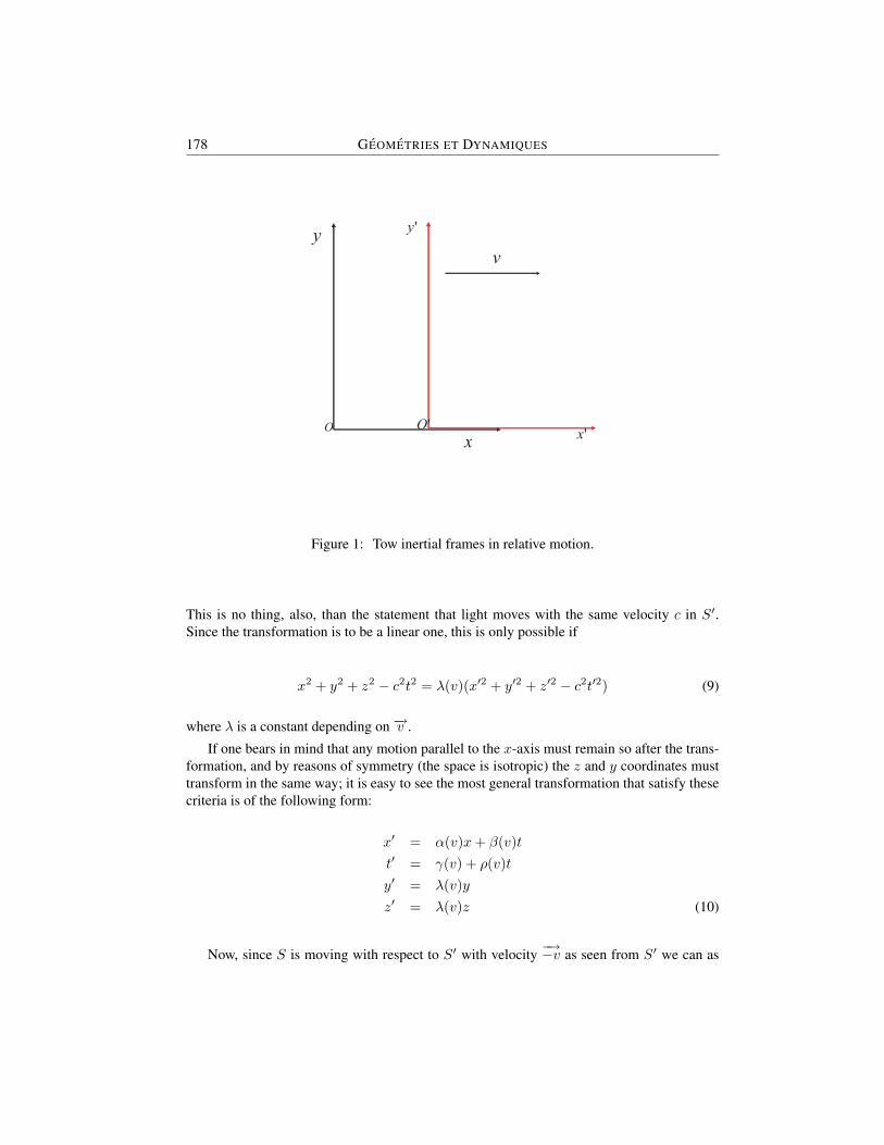
178 GEOMETRIES ET DYNAMIQUES
y
'y
O 'O
v
x'x
Figure 1: Tow inertial frames in relative motion.
This is no thing, also, than the statement that light moves with the same velocity c in S′.Since the transformation is to be a linear one, this is only possible if
x2 + y2 + z2 − c2t2 = λ(v)(x′2 + y′2 + z′2 − c2t′2) (9)
where λ is a constant depending on −→v .
If one bears in mind that any motion parallel to the x-axis must remain so after the trans-formation, and by reasons of symmetry (the space is isotropic) the z and y coordinates musttransform in the same way; it is easy to see the most general transformation that satisfy thesecriteria is of the following form:
x′ = α(v)x+ β(v)tt′ = γ(v) + ρ(v)ty′ = λ(v)yz′ = λ(v)z (10)
Now, since S is moving with respect to S′ with velocity −→−v as seen from S′ we can as

D. DOU 179
well write:
x = α(−v)x′ + β(−v)t′
t = γ(−v)x′ + ρ(−v)t′
y = λ(−v)y′
z′ = λ(−v)z′ (11)
From which it immediately follows that : λ(−→−v)λ(−→v ) = 1Now since all direction of space are equivalent than as far as the z and the y are concerned
there should be no difference whether the motion is with velocity −→v or −→−v. Hence
λ(−→−v) = λ(−→v )
which leads to λ(−→v ) = ±1, but λ(−→v ) must be positive (in the limiting case v = 0 we mustget λ(0) = 1), and we conclude that λ(−→v ) = 1.
Then a simple algebraic manipulation enables us to fix completely the value of α, β, γ, ρand show that the desired transformations are of the following form:
x′ =x− vt√1− v2
c2
t′ =t− (v/c2)x√
1− v2
c2
y′ = y
z′ = z (12)
This transformation is known as Lorentz transformation. It is clear from equation (3.6)that Lorentz transformations make sense only for velocities v < c, however we shall latershow that physical velocities can not exceed the velocity of light.
2. 5 Simultaneity, Lorentz Contraction and Time DilatationOne of the concepts that is taken for guarantee in the classical view of space and time isabsoluteness of simultaneity. Tow events located in different places in space are said to occursimultaneously if they happen at the same time, as measured in a given inertial system. Ifin a given inertial system S the space-time coordinates of events (1), say, are (t1, x1, y1, x1)and for event (2) are (t2, x2, y2, x2); if t1 = t2 the two events are said to be simultaneous.Consider another inertial system S′ moving with constant velocity in the x direction withrespect S. The space space-time coordinates of the two events in S′ are (t′1, x
′1, y′1, x′1) and
(t′2, x′2, y′2, x′2). Now, it is easy to see using Lorentz transformation that t′1 6= t′2 even if t1 =
t2, unless x1 = x2. Therefore, we conclude that tow events which are judged as simultaneousin one inertial system are not necessarily simultaneous in another inertial system. Indeed thisis one of the classical concepts, “absoluteness of simultaneity”, that one must abandon onedealing with relativity 6.
6Most of the paradoxes in special relativity are due to the failure of abandoning this concept.

180 GEOMETRIES ET DYNAMIQUES
Let us now consider some questions concerning the measurement of length of one andthe same measuring rod and of the duration of one and the same time in different inertialsystems.
Let S and S′ be two I.S, S′ is in translation motion with respect to S. Take a rod lyingalong the x-axis, at rest in S′(that is the rod is moving with velocity v with respect to S).
The positions coordinates of its ends x′1 and x′2 are thus independent of t′ and x′2 − x′1 =l0. l0 is the rest length of the rod or the proper length.
On the other hand, we might determine the length of the rod in the system S, in thefollowing way: We find x1 and x2 as a function of t. Then the distance between the twopoints which coincide simultaneously with the end points of the rod in S, will be called thelength l of the rod in the moving system , x2 − x1 = l. Since these two positions are nottaken up simultaneously in S′, it cannot be expected that l equals l0.
From Lorentz transformation
x′2 = γ(x2 − vt) , x′1 = γ(x1 − vt)
from which we obtain for ll =
√1− v2/c2l0
This states that the length of the rod in the system S appears shortened in the ratio√1− v2/c2 : 1.
Consider now a clock which is at rest in S′, the time which it indicates in S′ is its propertime τ and we can put its coordinates x′ equal to zero. It follows then from Lorentz transfor-mation that
t =τ√
1− v2/c2
Measured in the time scale of S, therefore, a clock moving with velocity v will lag behindone at rest in S in the ratio
√1− v2/c2 : 1.
In view of the relativity of the concepts of time and lengths, a question that is generallyraised is whether there is any thing real that can be associated with the lengths of rods or timedurations indicated by clocks. For instance one may argue that the proper length of a rod (inthe system where it is at rest) is the real length of the rod, and the other lengths measured bymoving observers are just apparent. The application of the distinction between “apparent”and “real” in this naıve sense is no more reasonable than asking what is the real x- coordinateof a point when it is not known which x− y-coordinate system is meant.
2. 6 On the Addition of Velocities and Causality
Having established the relation between space and time coordinates in different I.S’s, and theconsequences that this has brought on the notion of space and time; we can now go moredeep in the Kinematics of Relativity.
Our starting principle that led to the derivation of Lorentz was the failure of the old addi-tion law of velocity.
Let us now see how velocities are compounded in relativity.
D. DOU 181
Consider an object (point) moving in space, the position as measured in a given I.S S isgiven by (x(t), y(t), z(t). The velocity with respect to S is
−→u = (ux =dx
dt, uy =
dy
dt, uz =
dz
dt)
The velocity in with respect to S′ is
−→u′ = (u′x =
dx′
dt′, u′y =
dy′
dt′, u′z =
dz′
dt′)
Using Lorentz transformation we deduce
u′x =ux − v
1 + vux/c2
u′y =(1− v2/c2)uy
1 + vux/c2
u′z =(1− v2/c2)uz
1 + vux/c2(13)
Then it is easy to see that any body moving with velocity −→u with respect to S, such that|−→u | < c, will have velocity
−→u′ in S′ such that |
−→u′ | < c. In particular if |−→u | = c then |
−→u′ | = c
as expected.Hence the velocity of light is, kinematically, a limiting velocity which cannot be ex-
ceeded. However this is not enough, one could still argue that it is possible to acceleratebodies so that their speed will exceed that of light.What one really needs here is a dynamicalprinciple that would prevent velocity from exceeding that of light. We shall see later that thedynamics built upon relativity leads automatically to the physical impossibility to exceed thevelocity of light.
Now, suppose that it were possible that an effect in a system S is propagated with velocitygreater than the velocity of light. There would then exist a system S′ (moving relative to Swith velocity v less than c) in which event causing another, later, event in S would happenafter it.
To see this consider a motion in S with uy = uz = 0 and ux > c, than
u′x =uxv
1− uxv/c2< 0
by choosing c/ux < v/c < 1. This would be tantamount to upsetting the concept of causeand effect, and it can therefore be concluded that it is impossible to send any physical signalor effect with velocity greater than the velocity of light.
This is known as the causality principle, and it is sometime stated as part of the postulateof special relativity.
Before we move to the more geometrical interpretation of Relativity, it is of great interestto understand the relation between Einstein relativity and Newtonian relativity based on theconcept of absolute space and time.

182 GEOMETRIES ET DYNAMIQUES
In our daily life we never see moving clocks lagging behind static ones, or moving rodsappearing contacted with static ones; Newtonian mechanics and Galilean transformation de-scribe with great accuracy daily mechanical events. Of course relativity must provide ananswer for that, since by principle it should be a sort of refinement for the old view of spaceand time. Now, in our daily life we deal with motions with velocities that are negligible incomparison with the velocity of the light, that is v c. If we take this into account, Lorentztransformation can be approximated as follow
x′ = x− vt+O(v2/c2)t′ = t+O(v2/c2)y′ = y
z′ = z (14)
The deviation from Galilean transformation is of a second order in v/c, (v2/c2 = 10−10,for the fastest airplane on earth).
2. 7 Geometrical Interpretation of Lorentz Transformation
Since only the perpendicular component and time are affected by Lorentz transformation, weshall from now on restrict our attention to the (x, t) components to discuss the geometricalmeaning of these transformations.
Before discussing Lorentz transformation, it turns out to be conceptually useful to discussrotation in two dimensional Euclidean spaces R2, or 2-dimensional plan.
It is typically convenient to label coordinates by introducing the Cartesian coordinates.Consider now such a coordinate system (x, y), let p1 and p2 be two points in the plan
with coordinates (x1, y1), (x2, y2) resp.If a different Cartesian coordinate system is chosen, defined by x′ and y′ axes which are
rotated with angle θ with respect to the originals, the relation between the coordinates in theoriginal system and the rotated one are well known;
x′ = x cos θ + sin θy′ = −x sin θ + cos θ (15)
The points p1 and p2 will, of course, have different coordinates in the rotated system.Consider now the distance between the two points ∆s defined using the standard Eu-
clidean metric:
∆s2 = (x1 − x2)2 + (y1 − y2)2 (16)
Now it is easy to show that
∆s2 = (x′1 − x′2)2 + (y′1 − y′2)2 (17)

D. DOU 183
Although the coordinates change their values in moving from the original coordinate sys-tem to the rotated one, the distance is unaltered. We therefore say that the distance is invariantunder such changes of coordinates. This is a general future of geometry. Coordinates are notthe essence of geometry, coordinates are just number that we use to label each point. Theessence of geometry, or the quantities that really characterize the space, must be invariantunder change of coordinates.
The distance in the Euclidean plan is such an example of invariant quantity, that does notdepend on the choice of the coordinate. Here we must mention that the rotation we useddoes not only leave the distance invariant but leave the relation between the distance andcoordinate unchanged, they are both described by the same equation. The rotation is not onlya coordinate transformation but an isometry of the Euclidean metric in the plan.We will turnto this point more later, but it is important to keep in mind this distinction, rotations are justclass of a larger group of coordinates transformation.
t
x
'x
't
Figure 2: Geometrical representation of Lorentz transformation.
Now we are ready to investigate the geometrical interpretation of lorentz transformation.Consider a system of coordinate S endowed with cartesian coordinate (x, y, z, t), the
fact that we are able to describe globally the space and time by cartesian coordinates via theCartesian coordinates, therefore our space and time is just R4.
As mentioned earlier it will be sufficient for our purpose to consider only the two dimen-sional subspace R2 made of the x and t.
184 GEOMETRIES ET DYNAMIQUES
Consider then an inertial coordinate system S. Let (x, t) denote the space and time coor-dinates in this system.
If now we consider another coordinate system S′ that is moving with velocity v withrespect to S. The coordinates (x′, t′) of S′ are related to (x, t) by Lorentz transformation.
x′ =x− vt√1− v2
c2
t′ =t− (v/c2)x√
1− v2
c2
(18)
Let us know try to represent geometrically Lorentz transformation.We start by portrayingthe initial t and x axes at right angles, although this not necessary! The x′ axis is representedby the equation t′ = 0, then from equation (18) we get x = vt. The t′ axis is represented bythe line t = v/c2x.
The resulting picture is shown in fig 2. We therefore see that the space and time axesare rotated into each other, although they scissor together instead of remaining orthogonalin the traditional Euclidean sense.(As we shall see, the axes do in fact remain orthogonal inthe Lorentzian sense). This should come as no surprise, since if space and time behave justlike a four-dimensional version of space the world would be a very different place. It is alsoenlightening to consider the paths corresponding to travel at the speed of light c. These aregiven in the original coordinate system by x = ±ct. In the new system, these paths are stillgiven by x′ = ±ct′ and they are the same as those defined by x = ±ct; these trajectory areleft invariant under Lorentz transformations. Of course Lorentz transformation were derivedto do just that, the velocity of light is the same in all inertial coordinates systems.
Now in the Euclidean plan or in R3 in general, distances are invariant under rotation.A natural question that we should ask is: What is the invariant which characterizes Lorentztransformations?.
The answer to this question follows almost automatically from the derivation of Lorentztransformation. Consider two events in space and time characterized by the coordinates(x1, y1, z1, t1) and (x2, y2, z2, t2) and let ∆s2 be
∆s2 = (x1 − x2)2 + (y1 − y2)2 + (z1 − z2)2 − c2(t1 − t2)2 (19)
Now let us move to another inertial coordinate system obtained by Lorentz transforma-tion. The events (1) and (2) will now have the coordinates (x′1, y
′1, z′1, t′1) and (x′2, y
′2, z′2, t′2),
where the primed and unprimed coordinates are related by Lorentz transformation. Now it iseasy to show that although the coordinates change in moving from one coordinate system toanother, the interval defined by (19) remains invariant under change of coordinates, that is
∆s2 = (x1 − x2)2 + (y1 − y2)2 + (z1 − z2)2 − c2(t1 − t2)2
= (x′1 − x′2)2 + (y′1 − y′2)2 + (z′1 − z′2)2 − c2(t′1 − t′2)2

D. DOU 185
Thus we have obtained a quantity that is invariant and have a coordinate independentmeaning. The interval between the events defined in this way plays the role of distance inEuclidean geometry, and can be used to describe physical events in coordinate free manner.
One of the most fundamental consequences of the invariance of the interval is that itdivides the history of a given event into two causally disjoint regions.
To see this consider the origin (0, 0, 0, 0) and consider the set of points defined by thefollowing equation
x2 + y2 + z2 = c2t2
The sets of points satisfying this equation form two cones, one for positive times andother for negative times, the entire set is invariant under Lorentz transformation. Movementson each cone must occur with velocity of light.
Now, since light can be used as a mean of communication, events that occurred at negativetimes and lie on the cone can be transmitted to the origin and therefore affect it. That is tosay, those events with x2 + y2 + z2 = c2t2 and t ≤ 0 make part of the causal past of theorigin. Events with positive times are in principle reachable from the origin by light andcommunication is possible, therefore these events with x2 + y2 + z2 = c2t2 and t ≥ 0 makepart of the future of the origin. The set of points satisfying the equation x2 + y2 + z2 = c2t2
is called the light cone. The subset for which t ≤ 0 is called the past light cone, and the onewith t ≥ 0 is called the future light cone.
Consider now the set made of the points satisfying x2 + y2 + z2 < c2t2, this is theequation of a solid cone with the boundary removed. This set is also invariant under Lorentztransformation and are in principle reachable from the origin by signals that moves withvelocity less than the velocity of light. This set also splits naturally into two subset, positiveand negative times. The subset with positive (negative) makes part of the future (past) of theorigin. The points of this set are said to be time-like separated from the origin.
It remains now to consider the set of points outside the light cone. This set is made of thepoints that satisfy the following equation x2 + y2 + z2 > c2t2, which is also invariant underLorentz transformations. In order to communicate with this region one has to use signalsthat move faster than light, which is physically impossible, therefore this region is causallydisconnected from the origin. The points belonging to this region are said to be space-likerelated to the origin.
To sum up we have the following definitions:Let p1 and p2 be two events in space and time with coordinates (x1, y1, z1, t1) and
(x2, y2, z2, t2) and ∆s2 = (x1 − x2)2 + (y1 − y2)2 + (z1 − z2)2 − c2(t1 − t2)2, then:
• if ∆s2 ≥ 0, p1 and p2 are said time-like related.
• if ∆s2 = 0, p1 and p2 are said null related.
• if ∆s2 > 0, p1 and p2 are said space-like related.
The causal future (past) of the event p1 is the set of all the events with coordinates(x, y, z, t) satisfying (x1 − x)2 + (y1 − y)2 + (z1 − z)2 − c2(t1 − t)2 ≤ 0 and t − t1 > 0( t − t1 < 0), fig 3. Note here that the statements t − t1 > 0 and t − t1 < 0 are Lorentzinvariant.

186 GEOMETRIES ET DYNAMIQUES
Future Light Cone
Past Light Cone
t
x
ctx
ctx
Causaly disconnected
sector Causaly disconnected
sector
Figure 3: The different causal regions with respect to the origin.
At the end of this section it worth mentioning that one can use the geometrical repre-sentation of Lorentz transforation, depicted in fig 2, to derive length contraction and timedilatation. However in doing that, one must pay attention to a subtle point. In contrast to thestandard Euclidean rotation, Lorentz transformed axes i.e (x′, t′) have different calibrationfrom the original axes. One must use calibration curves of the form t2 − x2 = a (hyperbo-lae), which are invariant, in order to define the right calibration of the axes, and then comparedistance and time durations 7.
3 Minkowski Space and Lorentzian MetricLorentz transformations, in a sense, rotate space and time into each other. There is no absolutenotion of “simultaneous events”; whether two things occur at the same time depends onthe coordinates used. What may seem part of space for one observer seems a part of timefor another observer. Therefore the division of the physical world into space and time is achoice we make for our own purpose, not something intrinsic to the situation more than is thedivision of R2 into x and y direction. Our first conclusion is that we should really think ofspace and time as forming a four dimensional manifold. Our assumptions about the validityof global cartesian coordinates covering space and time lead us to conjecture that space andtime is globally R4. This is of course by no means an obvious conjecture, it is just an a prioriassumption from what we locally perceive about space and time.The map of space and timeinto R4 was called inertial coordinate system ( global).Many different coordinate systems arepossible and are related by Lorentz transformations.
7In the Euclidean plane the calibration curves are circles, x2 + y2 = a2, and those are invariant under rotationand they intersect the original and the rotated axes at the same distances from the origin

D. DOU 187
Now, generally a manifold may carry a further structure if it is endowed with a metrictensor, which is a natural generalization of the inner product between two vectors in Rn to anarbitrary manifold. With this new structure, we define an inner product between two vectorsin a tangent space of a given point.
A natural question to ask here is whether we can define a metric or a notion of distance onthis spacetime. It may seem tempting to use an Euclidean metric, however, a close inceptionshows that a distance defined using Euclidean metric will not be invariant under class ofcoordinate transformation i.e Lorentz transformation, and this is enough reason to excludethis possibility.
In discussing the geometrical interpretation of Lorentz transformation we concluded thatthere is a quantity that plays the same role of the Euclidean distance and remains invariantunder Lorentz transformation. This quantity was defined by
∆s2 = (x1 − x2)2 + (y1 − y2)2 + (z1 − z2)2 − c2(t1 − t2)2
If the two points are infinitesimal close we can write
ds2 = dx2 + dy2 + dz2 − c2dt2
if we denote x0 ≡ ct, x1 ≡ x, x2 ≡ y and x3 ≡ z we can write ds2,
ds2 = −dx20 + dx2
1 + dx22 + dx2
3 (20)
As far as the space components are concerned the distance is just the standard Euclideanmetric. The space time infinitesimal distance defined in this way is invariant under Lorentztransformation. However it is easily seen that this distance is not positive definite, thereforea metric defined in this way can not be an Euclidean metric. The fact we require a metricto be positive definite has no mathematical reason beside our experience of space distancebeing positive. Now we are facing another experimental fact, for space and time one can notdefine an Euclidean metric, but at the same time there is a natural metric that can be defined.Therefore we are going to take equation (20) as our starting point to introduce a metric andfor this we need to generalize the notion of metric.
Definition Let M be a differentiable manifold : A pseudo−Riemannian metric g onM is a type (0, 2) tensor field on M which satisfies the following axioms at each pint p ∈M :
• gp(U, V ) = gp(V,U).
• If gp(U, V ) = 0, for any U ∈ TpM then V = 0.
U, V ∈ TpM . In short, gp is a symmetric bilinear form.
Now since gµν(p) is still real symmetric matrix and has a maximal rank, it can be diag-onalized and all its diagonal elements reduced to ±1. If there are i positive and j negativeeigenvalues, the pair (i, j) is called the index of the metric. If j = 1, the metric is called aLorentz metric8.
In case (M,g) is Lorentzian, the elements of TpM are divided into three classes as follow,
8Some times one encounters another convention for Lorentz metric for which j = 3 and i = 1.

188 GEOMETRIES ET DYNAMIQUES
• g(U,U) > 0→ U is spacelike
• g(U,U) = 0→ U is null
• g(U,U) < 0→ U is timelike
The above division is made in accordance with our previous division of the interval be-tween events.
One can easily generalize all the mathematical objects (Curvature, Geodesics, integration,etc.) of Riemannian geometry to the pseudo-Riemannian one. From now on we shall assumethat this has been done.
Let us now consider the space time distance defined by equation (20). The metric associ-ated with this distance can be written in a given global inertial coordinate system as
gp =3∑
µ,ν=0
ηµνdxµ ⊗ dxν , ∀p (21)
where (ηµν) is given by −1 0 0 00 1 0 00 0 1 00 0 0 1
Before moving on let us introduce a very useful convention known as Einstein summationconvention: if the same index appears twice then the index is summed over all possiblevalues.
Using this convention equation (21) can be written as
gp = ηµνdxµ ⊗ dxν ,∀p (22)
Geometrically this means that: Space and time is the manifold R4 with a flat metric ofLorentz index defined on it. This space is called Minkowski space or world, and veryoften denoted M4, however we shall use (R4, η). The metric η is called Minkowski metric.
Now consider all the coordinates transformations that leave the spacetime distance invari-ant,
(x0, x1, x2, x3)→ (x′0, x′1, x′2, x′3)
ds2 = −(dx0)2 + (dx1)2 + (dx2)2 + (dx3)2 = −(dx′0)2 + (dx′1)2 + (dx′2)2 + (dx′3)2
Using the metric (η) this can be stated as:
ηµνdxµdxν = ηµνdx
′µdx′ν
Since η is the metric than it must transform as (0, 2) tensor
∂x′µ
∂xα∂x′ν
∂xβηαβ = ηµν (23)
But this is just the requirement that the transformation be an Isometry.

D. DOU 189
Consider now the Minkwoski metric and let us find all the set of transformations thatsatisfy equation (23) i.e all the isometries of η.
First it is easy see to that a simple class of such transformations are the coordinates shift
xµ → x′µ = xµ + aµ
where aµ is a set of four fixed numbers. This just a reflection of the homogeneity ofspace-time. Physically, it means no matter the place we chose to do our experiment theresults will be the same. The only remaining class of transformations is to multiply xµ by aspacetime-independent matrix:
x′µ = Λµνxν
where Λµν = ∂x′µ
∂xν .Using more conventional matrix notation,
x′ = Λx
with this notation equation (23) can be written as
η = Λ>ηΛ (24)
The set of all matrix which satisfy (24) form a group called Lorentz Group denotedL(4) or O(1, 3).
A simple examples of elements of this group are the following matrices
Λ =
±1 0 0 00 ±1 0 00 0 ±1 00 0 0 ±1
A less trivial example is the sub-group of three-dimensional space rotation. The matrix
of this subgroup have the following general form
Λ =(
1 00 R
)where R is 3× 3 matrix satisfying;
1 = RT1R (25)
The set of matrices which satisfy (25) is known as the orthogonal three dimensional groupO(3).
Let us now give a more systematic study of the group L(4).A 4 × 4 matrix generally has 16 independent elements, however as a consequence of
equation (24) a matrix Λ ∈ L(4) can be parameterized by 6 independent elements.Equation (24) tell us that
∀Λ ∈ L(4) =⇒ det Λ = ±1
The group O(1, 3) is indeed a Lie group, with a disconnected group manifold, the con-nected components can be obtained as follow. It is obvious that the subset of matrix with

190 GEOMETRIES ET DYNAMIQUES
det Λ = 1, form a subgroup. The subset of matrices with determinant equal to 1(−1) isdenoted by L+(4) (L−(4)). Moreover the subset L+(4) has a subgroup called the properhomogenous Lorentz group, defined by imposing on Λ the additional requirement
Λ00 ≥ 1 (26)
Note that from (24) we have,
(Λ00)2 = 1 +
3∑i=1
(Λi0)2 ≥ 1
From which it follows that: Either Λ00 ≤ −1 or Λ0
0 ≥ 1. Now, because it is impossible bycontinuous change of parameters to jump from Λ0
0 ≤ −1 to Λ00 ≥ −1, or from det Λ = −1
to det Λ = 1, we are led to consider four connected components of L(4).L↑+(4) = Λ|Λ0
0 ≥ 1, detΛ = 1 Proper Lorentz Group,L↓+(4) = Λ|Λ0
0 ≤ −1, detΛ = 1 improper Lorentz Transformation,L↓−(4) = Λ|Λ0
0 ≤ −1, detΛ = −1 improper Lorentz Transformation,L↑+(4) = Λ|Λ0
0 ≥ 1, detΛ = −1 improper Lorentz Transformation,
The improper Lorentz transformations involve either space inversion or parity P :
P : (x1, x2, x3 → −x1,−x2,−x3)
and therefore det Λ = −1 and Λ00 ≥ 1.
Or time reversal T :T : x0 → −x0
and therefore det Λ = −1 and Λ00 ≤ −1.
Both P and T transformation are known to be not an exact symmetry of nature, neither isthe product of P and T or PT . Indeed we can not go further in discussing the space reelectionand time reversal, since it will take us away from the main scope of these lectures9.
Now it is easily seen that the full Lorentz group is made up of the following four com-ponents: L↑+(4), PL↑+(4), TL↑+(4) and PTL↑+(4). In order to study the full group O(1, 3)it is enough to study the component connected to the identity and the discrete group made ofP, T i.e the connected component and the factor, which is always a discrete group.
Consider the proper Lorentz group L↑+(4) which is generally denoted SO0(1, 3) orSO0(3, 1).
Let Λ be an arbitrary element of SO0(1, 3), and let (α1, α2 · · · α6) be the six parametersneeded to parameterize the matrix. We chose these parameters such that,
Λ(α = 0) = I
9It is worth mentioning that although P and T are well defined concepts in classical physics, they acquire a par-ticular and fundamental role only in quantum physics; and indeed it is at this level where the P and T transformationfails to be a symmetry of nature.

D. DOU 191
Consider now an infinitesimal transformation (close to the identity). This obtained
Λ(δα) = I + δαiLi
where Li = ∂Λ(α)∂αi|α=0. That is Li belongs to the tangent space on the Lie group (which is a
manifold) : Li ∈ TeSO0(1, 3).Using the infinitesimal version of (24) we get
δαi(LTi η + ηLi) = 0
A solution of this equation is given by
L01 =
0 −1 0 0−1 0 0 00 0 0 00 0 0 0
L02 =
0 0 −1 00 0 0 0−1 0 0 00 0 0 0
L03 =
0 0 0 −10 0 0 00 0 0 0−1 0 0 0
L12 =
0 0 0 00 0 1 00 −1 0 00 0 0 0
L13 =
0 0 0 00 0 0 10 0 0 00 −1 0 0
L23 =
0 0 0 00 0 0 00 0 0 10 0 −1 0
The matricesLij are known as the generators of Lorentz transformation, they form a basis
of the Lie algebra of the Lie group SO0(1, 3).Consider for instance a transformation obtained from the identity by successive applica-
tion of the following transformation,
R(δθ) = I + δθL12
If we apply R(δθ) N -times we get
RN =N∏n=1
(I + δθL12)
If we define δθ = θN and let N →∞, we obtain the finite transformation
R(θ) = limN→∞RN = (I +θ
NL12)N = eθL12
A simple calculation leads to
R(θ) =
1 0 0 00 cos θ sin θ 00 − sin θ cos θ 00 0 0 1

192 GEOMETRIES ET DYNAMIQUES
This, of course, no more than a rigid rotation in x1−x2 plan. The same can be shown for L13
andL23 that they generate the remaining space rotations. In fact one can easily show that eachgenerator Lij generates one-parameter group of transformations. The one parameter groupsgenerated by L12, L23 and L23 are all compact (0 ≤ α ≤ 2π).
Now it remains to consider the generators L01, L02 and L03. It is sufficient to considerthe generator L01.
Consider again a finite transformation obtained from the identity by successive applica-tion of infinitesimal transformation,
Λ(δφ) = I + δφL01
Going through the same steps as for L12 we obtain for an arbitrary finite transformation,
Λ(φ) =
coshφ − sinhφ 0 0− sinhφ coshφ 0 0
0 0 1 00 0 0 1
(27)
Let us find the explicit form of the new coordinates
x′0 = x0 coshφ− x1 sinhφx′1 = −x0 sinhφ+ x1 coshφx′2 = x2
x′3 = x3 (28)
Let v/c ≡ tanhφ. It follows that −c ≤ v ≤ c. A simple algebra leads to
x′0 = γ(x0 − v
cx1)
x′1 = γ(−vcx0 + x1)
x′2 = x2
x′3 = x3 (29)
where γ = 1/√
1− v2/c2. But this is just Lorentz transformations between tow inertialcoordinate systems. Lorentz transformation looks like a rotation in t−x plan, and the velocityplays the role of the tangent of the angle φ (v = c tanhφ).
Now the essence of Special Relativity can be stated as follow:Space-time is R4 withflat Lorentzian metric defined on it. Of course all coordinate systems are equally good forthe manifold R4, however there is privilege given to the global coordinate systems (inertialcoordinate systems) in which the metric take the form (22). Now, the relativity principlewould be no thing more than requiring the physical laws to be invariant under isometries.Isometries are from the point of view spacetime the symmetry of the manifold, and justspecial class of coordinate transformations, hence Special Relativity.
The Lorentz and spacetime translation transformations form a group called Poincaregroup. A general transformation of Poincare group is of the following form

D. DOU 193
xµ → x′µ = Λµνxν + aµ
where Λ ∈ SO0(3, 1).Note that Poincare group is not a direct product of Lorentz group and Translation group,
however, it is a semi-direct product.
3. 1 A bit of Relativistic MechanicsNote that starting from this section on we shall set the velocity of light equal to one: c = 1.
Let us remember that the starting point of the whole scheme was the study of motion ofbodies in space and time. Having established that the physical space to which the motionmust be referred to is a 4 dimensional space with flat Lorentzian metric (R4, η), we can nowstart building the dynamical equations that govern motions and at the same time respect theprinciple of special relativity. It turns out that with the help of Minkowski geometry thoserelativistic dynamical laws can easily be constructed using the principle of inertia and somelaws which survived from Newtonian mechanics. It is interesting here to mention that thelaws electromagnetism fitted automatically into scheme of the vector and tensor calculus in(R4, η), this of course should not be surprising, it is the theory of light that led us to specialrelativity.
Kinematics and Dynamics
In order to formulate the new mechanics we should remember two facts:
• Physical quantities must be represented by : Scalars (0-forms), vectors or co-vectors,tensors fields in (R4, η).
• The equations of motions must be invariant under Lorentz transforation i.e they takethe same form in all inertial coordinate systems.
The fact that we require the laws to be invariant under Lorentz transformations gives asort of privilege to the metric (η) and allows it to appear explicitly in the law of physics. Forinstance an tensorial equation of the form
∂µTν + ∂νTµ = ηµνφ
is acceptable. Tµ are the components of a co-vector field (one form) and φ is a scalar function(a zero-form).
A single particle in space-time will have trajectory which we will call a world line orpath.
A world line is specified by a curve i.e. map R → M4 , where R4 is our Minkowskispace. Let λ be an allowable parameterization of the curve representing the world line. Thetangent vector to this curve is V
V =dxµ
dλ∂µ

194 GEOMETRIES ET DYNAMIQUES
An object of primary interest is the norm of the tangent verctor, which serves to char-acterize the path; if the tangent vector is timelike/null/spacelike at some parameter value λ,we say that the path is timelike/null/spacelike at the point.This explains why the same wordsare used to classify vectors in the tangent space and intervals between two points, because astraight line connecting, say, two time-like separated points will itself be time-like at everypoint along the path. Moreover two points joined by a path which timelike/null/spacelikeevery where are timelike/null/spacelike separated. However classification of finite intervalsbetween points in timelike/null/spacelike is not generally meaningful (in curved spaces); itdepends on a specific choice of path (a “straight line”) which connects the points, and thischoice in turn depends on the fact that spacetime being flat.
A more natural object is the line element of an infinitesimal displacement: xµ → xµ+dxµ
ds2 = ηµνdxµdxν
From the definition it seems natural to take the square root and integrated along a path toobtain a finite interval. But since ds2 needs not be positive, we define different proceduresfor different cases. For space-like paths we define the path lentgh
4s =∫ √
ηµνdxµ
dλ
dxν
dλdλ
where the integral is taken over the path. However the path length is of a little interest forphysics.
For time-like paths we define the proper time
4τ =∫ √
−ηµνdxµ
dλ
dxν
dλdλ (30)
which will be positive. For null paths the interval is zero, so no extra formula is required.Notice that the integral of the line element is independent of the parameterization. We mayconsider paths that are time-like in some places and space-like in others, but fortunately itturns out that paths of physical particles never change their character, they always move ontime-like or null paths.
We used the word “proper time” for the line element integrated along a time-like curve,which is especially appropriate, since we shall shortly show that τ actually measures the timeelapsed on a physical clock carried along the path.
Consider a particle moving with velocity −→v (t) in a given inertial coordinate system. Thecoordinates of the particle are x0 = t, x1, x2, x3, the velocity is given by
vi =dxi
dx0=dxi
dt, i = 1, 2, 3
Consider an infinitesimal displacement of the particle between an instant t and t+ dt (x0
and x0 + dx0) as measured in the inertial system. Then d−→x = −→v dtBetween t and t+dtwe can consider the motion of the particle as rectilinear and uniform.
Consider now the coordinate system moving with the particle as inertial system, call it S∗
(generally called a co-moving frame). The space coordinates of the particle in S∗ are (0, 0, 0),

D. DOU 195
the time measured by the clock moving with the particle between the instant t and t+ dt willbe dt∗.
Now we can apply Lorentz transformation between the coordinate (dt, d−→x ) in the originalinertial system and the coordinates (dt∗,
−→0 ) in S∗ during the time t and t+ dt to obtain dt∗.
dt =dt∗√1− v2
(31)
it follows then
(1− v2)dt2 = (dt∗)2 = (1− d−→x 2
dt2)dt2 = dt2 − d−→x 2 =⇒
dt∗ =
√−ηµν
dxµ
dλ
dxν
dλdλ = dτ
So really dτ presents the proper time measured by a clock moving with particle. Note herethat we do not require the particle to move with rectilinear and uniform velocity, we requireit only to move along a timelike paths. It is interesting to note the proper time correspondingto a particle moving along a null path (with the velocity of light) is zero i.e the particle doesnot feel the passage of time!!.
Since the proper time is the time measured by a clock travelling on the timelike world-line, it provides a natural parameterization of timelike paths. If τ is used to parameterize thepath then the tangent vector is called the four− velocity, Uµ;
Uµ =dxµ
dτ(32)
Since dτ2 = −ηµνdxµdxν , the four-velocity is automatically normalized:
ηµνUµUν = UµUµ = −1 (33)
In the rest frame of the particle, its four-velocity has the components U = (1, 0, 0, 0).To have a flavor for why the name four-velocity is used, consider the case where the
particle is moving with small velocity compared to the velocity of light i.e v 1. In thiscase
U i =dxi
dτ=
1√1− v2
dxi
dt=dxi
dt+O(v2) ≈ vi
which are the components of classical velocity.Let us now consider Newton’s second law, which we wrote before as
d−→pdt
=−→F (34)
Although this law was one of the building stone of special relativity, it can not be thecorrect law for a simple reasons; it is not invariant under Lorentz transformation. This isobvious, since for a physical law to be invariant under Lorentz transformation it must be a

196 GEOMETRIES ET DYNAMIQUES
vector or tensorial equation. Nevertheless, it turned out that equation (34) in its current formhas enough information to lead us to the correct law.
One can show, using equation (34), the classical differential definition of energy andLorentz invariance, that the energy of the particle of mass m and the momentum combinetogether to form a four-vector given by
pµ = mUµ
With the energy E = p0 and the momentum −→p = (p1, p2, p3). An alternative way toexpress the energy and momentum is
E = M−→p = M−→v
(35)
where M is now defined byM =
m√1− v2
Let us know go back and consider the Newton’s second law. In order to generalize New-ton’s law we must take into account only tow things 1) it must be invariant under Lorentztransformation. 2) it boils down to Newton’s classic law in the limit of small velocities.
First we have to admit the existence of a four-vector fµ representing the force. Since theforce, by definition, measures the variation of momentum we are immediately led to considerthe following generalization
dpµ
dτ= fµ (36)
Consider the spacial part of this equation
d−→pdτ
=−→f
this is of course the same equation as the classical one for small velocities. To compare thisequation with the classical law, we use the time measured in the inertial system instead of theproper time
d−→pdt
=−→F
where−→F =
√1− v2
−→f is the analogue of the classical force.
Using the expression of −→p we can write
dM−→vdt
=−→F
Because M = m√1−v2 then it diverges as v approaches the velocity of light, therefore we
can never accelerate a particle so that its speed reaches or exceeds the velocity of light (wewould need an infinite force or energy!). We conclude that the speed of light is a limitingvelocity as a consequence of a relativistic dynamical principle and therefore massive particlewill always move on timelike paths.

D. DOU 197
Principle of Least Action and Energy Momentum Tensor
The extreme development of mechanics led to one principle that governs all the classicalphysics (non-quantum). This principle is known as the principle of least action. It can bestated in the following way: For each physical system there exits a function called lagrangianL and the action between tow instants of time t1 and t2 is a functional defined by
S =∫ t2
t1
Ldt (37)
The explicit form of the lagrangian depends on the system under consideration.Now the principle of Least action states that among all the possible paths the system
follows the path for which the action is an extrema. That is
δS = 0
The simplest system that may illustrate this principle is a single particle in one spacedimension. The lagrangian of this system is a function of the position x, the velocity dx
dt = xand time. Let us find what trajectory or path the particle will follow to go from a point x1 att = t1 to another point x2 at t2.
The action between this two points along a given path is given by
S[x] =∫ t2
t1
L(x, x, t)dt
Consider an infinitesimal variation δx(t) of the path with the end points kept fixed i.eδx(t1) = δx(t1) = 0.
The action along the deformed path is given
S[x+ δx] =∫ t2
t1
L(x+ δx, x+ δx, t)dt = S[x] + δS[x]
The variation of the action δS[x] can easily be derived
δS[x] =∫ t2
t1
[∂L∂x− d
dt
∂L∂x
]δxdt
If we require the variation to vanish for arbitrary infinitesimal deformation (extremize) weobtain
d
dt
∂L∂x− ∂L∂x
= 0 (38)
This is the Euler-Lagrange equation of motion.To see that this really gives the standard equations of motion consider a free a particle i.e
a particle with no external force acting on it.The lagrangian of this particle is given by its Kinetic energy (classic)
L =12mv2 =
12mx2 (39)

198 GEOMETRIES ET DYNAMIQUES
Euler-Lagrange equation givesmx = 0
which is the standard equation of motion of free particle. Quite generally the Lagrangian isdefined to be
L = T − Vwhere T is the Kinetic energy and V is the potential energy.
The most important application of the principle of least action is that it furnishes a naturalsetting for the conservation laws. Conservation laws are very powerful tool in physics and arenaturally related to the symmetry of the physical system. A symmetry of a physical system istransformation of the coordinates or the dynamical variables that leaves the action invariant.For instance if the action is invariant under time translation t→ t+ s where s is an arbitraryconstant, it follows from the action principle that energy is conserved. If the action is invariantunder space translation, that is xi → xi + ai, the action principle tells us that momentummust be conserved.
This is indeed a special case of a more general theorem known as Noether′s theorem,which states that to each continuous symmetry of the action (invariance) there is a conservedquantity Q i.e dQ
dt = 0.In general physics deals with fields (not a single particle), and we speak about Lagrangian
density to describe the dynamics of the fields. In this case the action is given by
S =∫ ∫
dtd3xL(φ, ∂φ)
where φ is the field variable. For a relativistic field theory, one can show that invariance underspace and time translation leads to the following equation
∂µTµν = 0 (40)
Tµν are the component of a symmetric tow rank tensor called the energy-momentumtensor. The components T 0µ can be shown to be the density of energy and momentum i.eT 0µ = ρUµ, where Uµ is the four velocity field. What is important about this is the follow-ing:
The total Energy and momentum of the field are given by
Pµ =∫d3xT 0µ
where the integral is taken over all the space. Using equation (40) and assuming that theenergy momentum “vanishes at space infinity”, one can easily show that
dPµ
dt= 0
this is energy and momentum conservation.Indeed, it is difficult to explain in few words the physics behind this definition of energy
momentum tensor, however intuitively we can understand the physical meaning as follow.Imagine that you have a distributions of matters or particles “fluid”, with a given density,each particle has his own four-velocity, and there will be pressure exerted by different partsof the fluid. The energy-momentum tensor is just the right quantity to describe the distributionof velocity and matter and pressure.

D. DOU 199
3. 2 GeodesicsIn Relativistic as well as in Classical Mechanics free particles move on straight lines in inertialcoordinate systems. As we mentioned earlier the equation of the path that a body follows fromone point to another is governed by the principle of least action. An immediate question thatarises is whether we can formulate a relativistic version of the principle of least action.
It turns out that for free particle there is already a geometrical interpretation of the princi-ple of least action. To see that, let us take first Minkowski space and try to construct an actionanalogue to (39) such that it gives the equation of motion (straight line). In doing so we haveto remember that the lagrangian must boils down to the classical one for small velocity andbe invariant under Lorentz transformation (scalar), otherwise the equations obtained woulddepend on the particular choice of the inertial coordinate system.
Now equation (39) suggests that we take as a lagrangian:
L = −αηµνdxµ
dτ
dxν
dτ
where α is still unknown parameter inserted to get the units right (the lagrangian has unitsof energy). This Lagrangian in the limit of small velocities coincides with non-relativistic oneup to an additive constant, which does not affect the equations of motion, given that we choseα = m (the mass of the particle). By variation the action of this lagrangian, it is easy toobtain
d2xµ
dτ2= 0
Beside this action there is another alternative one which satisfies all the desired criteria.Take as an action between two points the proper time itself (proportional to the world line),that is
S[x] = α
∫ λ2
λ1
√−ηµν
dxµ
dλ
dxν
dλdλ (41)
Variating this action (the proper time) and setting the variation to zero we obtain
d2xµ
dτ2= 0 (42)
which is the same equation we obtained using the other action. In fact the two action areequivalent, however one is more convenient than the other. For instance the action definedas the proper time has the simple geometrical interpretation but it is nonlinear, however forpractical calculation the first action is more convenient.
The variational principle provides a natural setting to rediscover the analogue of straightlines in curved spaces (space-times), namely Geodesics.
Given spacetime with metric g. Consider the proper time functional,
τ = α
∫ √−gµν
dxµ
dλ
dxν
dλdλ (43)
To seek the extrema of this functional we introduce an infinitesimal variation of the curve
xµ → xµ + δxµ

200 GEOMETRIES ET DYNAMIQUES
this of course will introduce a variation on the metric (we changed the path of integration),
gµν → gµν(x+ δx) = gµν(x) + δxα∂αgµν
A straight forward calculation leads to
δτ =∫
[−12∂ρgµν
dxµ
dτ
dxν
dτ+
d
dτ(gµρ
dxµ
dτ)]δxρdτ
Since we are searching for stationary curve, we demand δτ to vanish for any variation; thisimplies (after some algebra)
d2xα
dτ2+
12gαβ(∂νgβµ + ∂µgβν − ∂βgµν)
dxµ
dτ
dxν
dτ= 0 (44)
This is precisely the geodesic equation, but with the specific choice of Christoffel sym-bols, namely the one compatible with the metric, called the Levi-Civita connection.
Γαµν =12gαβ(∂νgβµ + ∂µgβν − ∂βgµν) (45)
Using the definition of covariant derivative or the connection we can write the geodesicequation as
∇UU = Uµ(∇U)µ = 0 (46)
Where Uµ = dxµ
dτ are the components of the tangent vector of the geodesic. Equation (46)means that the tangent vector to the curve is transported parallel to itself.
Thus on a manifold with metric, extremals of the length functional are curves whichparallel transport their tangent vector with respect to Levi-Civita connection. From now onwe shall refer only to Levi-Civita connection.
Some remarks about the geodesics in Lorentzian spaces are in order:
• An important property of geodesics in a manifold with Lorentzian metric is that thecharacter timlike/null/spacelike of the geodesic never changes. This is true becausetransport preserves inner products (the metric is covariantly constant∇g = 0), and thecharacter is determined by the inner product of the tangent vector with itself.
• There are also null geodesics, which satisfy the same equation, except that the propertime cannot be used as a parameter.
• On a manifold with a Riemannian metric, one can always find curves of arbitrarily longlength connecting any two points. However, the length will be bounded from below,and the curve of shortest length connecting two points is necessarily an extremum oflength and thus geodesic. Thus, the shortest path between two points is always the“straightest possible path”. However, a given geodesic connecting two points needsnot be the shortest path (think of S2). In analogy with Riemannian spaces one maybe inclined to think that geodesics are curves which minimize the proper time, whichis uncorrect. For Lorentzian manifold, given two points that can be connected by atimelike curve, one can always find timelike curves of arbitrarily small proper time

D. DOU 201
connecting the points. Timelike geodesics cannot therefore be curves of minimumproper time, they are extrema. Again, given tow points, it is often possible that there ismore than one geodesic between them, so really we should speak about local extrema10.
4 General Relativity
4. 1 Invariance Under General Coordinate transformations
The reader may have felt unsatisfied with the fact that special relativity makes a distinctionbetween different coordinate systems. A privilege is given to Inertial Systems and coordinatetransformations which are isometries of the metric (lorentz transformation), whereas in dif-ferential geometry all coordinates system are equally good in describing the manifold. Fromthe pure geometrical of view, inertial coordinate system being special only for the fact thatgeodesics on this coordinates are straight lines. Viewed in this way the principle of specialrelativity ( Lorentz transformation) is really about symmetries of the spacetime and not aboutcoordinates transformation.
The physical principle that enables us to single inertial systems out of all the possiblecoordinates systems, is the principle of inertia and the constancy of the velocity of light. Nowafter we reached an understanding of the geometrical structure of space time as a metric spaceof a specific signature, the constancy of the velocity of light is just a geometric consequenceof the fact that light moves on null (geodesics) curves, and those are invariant. Nevertheless,so far the principle of inertia keeps the same status in special relativity as in Newtonianrelativity, and the distinction between inertial and non-inertial systems can not be drooped.Nonetheless from a purely geometrical point of view there is no thing that can prevent usfrom writing the laws of physics in an arbitrary coordinate system. Indeed, from childhoodwe have become familiar with the appearance of physical equations in non-Cartesian systems,such as polar coordinates, and in non inertial systems, such as rotating coordinates. In factfrom the physical viewpoint, all physical measurements amount to determining space-timecoincidences; nothing apart from these coincidences is observable.
At this stage, it may seem that writing the laws of physics in an arbitrary coordinatesystem will not add any thing new to the physical content of the theory, nevertheless it willprove very powerful for understanding of the subsequent development. For this reason weshall try to write some laws of relativity in an arbitrary coordinate system.
The most useful law, which stems its origin from the principle of inertia, is the relativisticversion of Newton’s law in the case where no forces are present (a body left to itself). Theequation of motion is just the geodesic equation with zero Levi-Cevita connection coefficients(in an inertial system).
d2xµ
dτ2= 0 (47)
Let us consider now an arbitrary coordinate transformation, not necessarily Lorentz transfor-
10However, a given geodesic needs not maximize the proper time between two points i.e existence of conjugatepoints

202 GEOMETRIES ET DYNAMIQUES
mation.xµ → x′µ
under such transformation the metric transforms to
gµν(x′) =∂xα
∂xµ∂xβ
∂xνηαβ
and equation (47) takes a different form
d2x′µ
dτ2+dx′α
dτ
dx′β
dτ
∂xµ
∂xσ∂2xσ
∂x′α∂x′β= 0 (48)
equation (48) is different from (47) only by the term dx′α
dτdx′β
dτ∂xµ
∂xσ∂2xσ
∂x′α∂x′β, however this
term can be related to the Levi-Civita connection coefficients of the metric gµν(x′). In fact∂xµ
∂xσ∂2xσ
∂x′α∂x′βare just the connection coefficients resulting by coordinate transformation from
a vanishing connection coefficients. Therefore we can rewrite equation (48) using covariantderivative and bring it to a coordinate independent form. In arbitrary coordinate system
∇UU = 0 (49)
this equation is manifestly invariant under all coordinate transformation. The fact that theycan be reduced to the standard form of equation (47) is due to the existence of global coor-dinate system in which the metric is reduce to the flat one with vanishing connection coeffi-cients.
Equation (49) teaches us a very important lesson. In classical mechanics when non-inertial systems is used terms similar to dx′α
dτdx′β
dτ∂xµ
∂xσ∂2xσ
∂x′α∂x′βare interpreted as forces gen-
erated by the relative motion with respect to the inertial system (relative acceleration, Coriolisforce, ...) however from the geometrical point of view there is no difference between the equa-tion (49) and (47). The extra terms that appear in (49) are just due to the non-vanishing ofthe connection coefficients in this coordinate system.
Along this line we can easily rewrite all the laws of special relativity in general covariantform i.e they take the same form in all coordinate systems, by just subsisting for the metriccomponents their form and for the derivative the covariant derivatives (we take into accountthe non-vanishing of the Levi-Civita coefficients). Now, at least from the geometrical pointof view, inertial system lost their privilege, and the law of physics can be brought into such aform that they read the same in every coordinate system, i.e they are covariant under arbitrarycoordinate transformations. This is achieved by incorporating the correct metric (along withits connection coefficients) into the physical laws.
Now the generalization of the principle of special relativity (invariance and Lorentz trans-formation) will not bring any thing new as long as we are able to find global coordinate sys-tem in which the metric is flat. Therefore we have reduced the principle of relativity to theexistence of global inertial systems.
4. 2 Locally Flat Coordinate System-Locally Inertial SystemIn discussing the formulation of the law of special relativity in general covariant form, weconcluded that it is the existence of global coordinates systems which makes the invariance

D. DOU 203
under general coordinates transformation of little value from the physical point of view. How-ever there is a fundamental point that must be discussed here. Most of our statement aboutspace time are usually affected by our local measurement which can hardly capture the globalstructure of space-time.
So let us discuss this point from the geometrical point of view. Let (M,g) be (pseudo)-Riemannian manifold with an arbitrary metric. Let p be an arbitrary point of the manifold,let gµν(p) be the components of the metric at the point p which are in general different fromηµν . One can show (some how easily) that there always exists a coordinate system xµ whoseorigin is at p and in which:
g′µν(x) = ηµν + 0(x2) (50)
∂αg′µν |p= 0⇒ Γ′αµν(p) = 0 (51)
That is, the metric near p is approximatively that of special relativity, differences being ofsecond order in the coordinates and can be shown to be directly proportional to Riemanncurvature tensor at the point p.
Moreover one can also show that this coordinate system is not unique but defined up toLorentz transformation (which is expected). One may hope to do better and go beyond thesecond derivative, however, it turns out that it is generally impossible to go beyond the firstderivative. The reason of not being able to make the second derivative vanish by coordi-nates transformation is due to the direct relation between Riemann curvature and the secondderivatives of the metric, which is non zero for curved spaces.
So although we are generally unable to find a coordinate system in which the metric takethe canonical form, we can always find a coordinate system such that, in the first neighbor-hood of given point the metric looks like that of flat space. This is merely the statement thatany manifold has a flat space ‘tangent’ to it at any point. Such coordinates are known as ‘lo-cal flat coordinate Systems’ or Riemann normal coordinates and in the context of Lorentziangeometry is referred to as ‘local Lorentz or Inertial frames’11.
Recall that straight lines in flat space are the world lines (spacetime path) of free particle;the absence of the first derivative terms in equation (50) will mean that free particles aremoving on paths that are locally straight in this coordinate system.
In physical terms,“a small enough region of space-time looks like Minkowski space andfree particle in this region will move on straight lines”. The question of how small or big thisregion depends of course on the smallness and the largeness of the region in comparison ofthe curvature.
4. 3 The Principle of EquivalenceLet us now remember that our point of departure was the principle of inertia, which statesthat body left to itself will move with rectilinear and uniform motion, the coordinate systemsin which this law is true are inertial systems.
Now acceleration in inertial systems is generated by forces and governed by Newton’ssecond law
mi−→a =
−→F (52)
11The reason for this terminology will become clear later.

204 GEOMETRIES ET DYNAMIQUES
The inertial mass has a universal character, related to the resistance you feel when youtry to push on the object; it is the same no matter what kind of force is being exerted. Besidethe inertial mass, there is to each body a gravitational mass defined as the source of thegravitational force. For instance we are well aware of the fact that all objects are attractedto the earth. The force exerted by the earth on an object is the gravitational forces Fg . Thegravitational force is the mutual of attraction between any two objects in the universe. The lawthat governs this force is Newton’s third law, which states that every particle in the universeattracts every other particle with a force that is directly proportional to the product of the twogravitational masses and inversely proportional to the square of the distance between them.If two particles have gravitational masses Mg and mg and are separated by a distance r themagnitude of the gravitational force is
−→Fg =
GmgMg
r3−→r (53)
where G is the universal gravitational constants.A more precise and general formulation of this law is the following. If we have an arbi-
trary distribution of matter such that the density of the gravitational mass is ρ(−→r ), than theforce exerted by this matter on a test body of gravitational mass mg is given by
−→F g = −mg
−→∇φ = −mg
−→g (54)
where φ is called the gravitational potential which satisfy Poisson equation
∇2φ = 4πGρ (55)
where∇2 = δij∂j∂j is the Laplacian in space. −→g is called the gravitational field.Now if we apply Newton’s second law to this test particle we get
mi−→a =
−→F g = mg
−→g (56)
where mi is the inertial mass.Now, so far there seems no thing special about gravitational forces, they seem like any
other force i.e electromagnetic..etc. However in contrast to the electric, magnetic and otherforces in nature, the gravitational field exhibits a remarkable property, which is of funda-mental importance for what follows. Bodies which are moving under the sole influence ofgravitational field receive an acceleration, which does not in the least depend either on thematerial or on the physical state of the body. For instance, a piece of lead and a piece of woodfall in exactly the same manner in gravitational field (in vacuo), when they start off from restor with the same initial velocity. This law, which holds most accurately, can be expressed ina different form on the light of the following consideration12
According to Newton’s law (56), we have
(Force) = (inertial mass)× (acceleration)
12These consideration are taken, with slight modifications, from Einstein’s book: Relativity, the special and thegeneral theory.

D. DOU 205
If now gravitation is the cause of the acceleration, we then have
(Force) = (gravitational mass)× (intensity gravitational field)
From this two relations follows:
(acceleartion) =(gravitational mass)
(inertial mass)(intensity of the gravitational field).
Now, experience tells that all objects fall with the same accelerations in a given gravitationalfield, independent of the composition of the object, then the ratio of the gravitational and theinertial mass must likewise be the same for all bodies. By suitable choice of units we can thusmake this ratio equal to unity. We then have the following law: The graviational mass ofa body is equal to its inertial mass. This sometimes refereed as the Weak EquivalencePrinciples: The inertial mass and the gravitational mass of any object are equal.
Now armed with this principle, we can rewrite our previous equations
m−→a = m−→g (57)
where we removed the subscripts.The equality between inertial and gravitational has a far reaching and profound conse-
quences.Imagine that a man “physicist-observer” is enclosed in a big box (room) with a ball on his
hand and unable to observe the outside world. Suppose also that the system (Box+Man+Ball)is so far removed from the stars and other appreciable masses, that the law of inertia appliesquite accurately: objects at rest remain at rest and objects in motions continue permanentlyin uniform rectilinear motion. Viewed as a reference, the system is an inertial system. Let usnow suppose that a hook with rope attached and the box is pulled with constant force. TheB.M.B will then begin to move “upward!” with a uniformly accelerated motion.In course oftime their velocity will reach unheard-of value- provided that we are viewing all this fromanother reference body which is not being pulled with the system fig 4.
But how does the physicists in the box regard the process? The acceleration of the boxwill be transmitted to him by the reaction of the floor of the box. “He takes up this pressureby means of his legs”. He is then standing in the box in exactly the same way as anyonestands in a room of a house on our earth (provided that it is exactly equal to that of theearth acceleration). Now if he releases the ball which he previously had in his hand, theacceleration of the box will no longer be transmitted to this ball, and for this reason the ballwill approach the floor of the box and accelerated relative motion. The observer (the man)will further convince himself that the acceleration of the body towards the floor of the box isalways the same magnitude; whatever kind of body he may happen to use for the experiment.Now, relying on his knowledge of gravitational field, the man in the box will thus come tothe conclusion that he and the box are in gravitational field which is constant with regardto time.Of course he will be puzzled for a moment as to why the box does not fall in thisgravitational field. Just then, however, he discovers the hook in the middle of the lid of thebox and the rope which is attached to it, and he consequently comes to the conclusion thatthe box is suspended at rest in the gravitational field. Even though it is being accelerated withrespect to the inertial system first considered, we can nevertheless regard the box as being at

206 GEOMETRIES ET DYNAMIQUES
F F
Force = acceleration
NO Gravity g=0
Figure 4:
rest in a gravitational field. Of course, there is still an alternative possibility of the processwhich is the real situation, however, the question that ought to ask is :Is there any means ofdistinguishing by experiment within the box between the two possibilities?
We are bound to answer that physics knows of no such means. Actually, the effect ofgrivation can in no way be distinguished from the effect of acceleration; each is fully equiv-alent to other, and this is what equation (57) is saying. Let us consider further our system(box+physicist) but now assume that he is holding two balls instead of one. Now suppose thatthe system is in free full towards the earth and the gravitational field assumed uniform, and askhow would the life for the physicist inside the box look like? What will the physicist noticeif he releases the two balls. Since they all are in free fall, with the same acceleration, he willnotice that the two balls remain in the same position, at rest with respect to him, moreover ifone ball is given an initial velocity it will continue to move rectilinearly and uniformly withthe same initial velocity. Remember also that the physicist does not feel any kind of pressurefrom the floor, they all fall with the same velocity. The first conclusion that the physicist willmake will be that he is an inertial system, since the law of inertia holds. Second he can by nomeans discover that he is in free fall under the action of a gravitational field (of course untilhe reaches his destiny and hits the ground of the earth).
This is essentially because of the circumstance that all bodies fall equally fast. The factthat we are unable to distinguish the two concepts acceleration and gravitation make theircoexistence very similar to the notion of absolute rest, which is a sort of unascertainable fact.Physics refuses to accept such concepts and statements and replaces them by new ones. Onlyascertainable facts have physical reality.
Classical mechanics distinguishes between the notion of a body that is left to itself sub-ject to no force (inertial motion) and the motion of a body under the action of gravitation.The former is rectilinear and uniform in an inertial system; the latter occurs in curvilinearpaths and is nonuniform. According to the principle of equivalence this distinguish must bedropped. For by merely passing over to an accelerated system of reference we can transform

D. DOU 207
the rectilinear of inertia into a curved, accelerated motion which cannot be distinguished fromone produced by gravitation. The converse holds too, so far for uniform gravitational fields.The theorem that the inertial motion relative to inertial system is uniform and rectilinear -theordinary law of inertia-now comes to an end.
Before we move further and state precisely the principle of equivalence let us transformthe previous remarks to explicit calculations.
Let S be an inertial system, if there exists a uniform gravitational field −→g (constant inspace and time) it will produce an acceleration for any object, the equation of motion of abody of mass m with respect to S is
m−→a =−→f +m−→g (58)
where−→f is the net force acting on the particle other than gravitational force.
If we move to an accelerated system S′ with acceleration −→γ with respect to S equation(58) take the following form
m(−→a′ +−→γ ) =
−→f +m−→g (59)
which can also be written asm−→a′ =
−→f +m(−→g −−→γ ) (60)
where−→a′ is now the acceleration of the body with respect to S′. By choosing −→g = −→γ we
reduce equation (60) to the standard form of a body under the action of a force−→f ; if
−→f = 0
the body will move uniformly and rectilinearly . We may say in general that by acceleratingthe system appropriately we can produce constant gravitational field, reduce one that is given,or annul, intensify, or reverse it.
Earth
Figure 5: The tidal force effect.

208 GEOMETRIES ET DYNAMIQUES
Now in reality gravitational field produced by the simplest distribution is not uniform or atleast homogenous. The intensity of the gravitational field varies from point to point in spaceand may also depend on time; therefore we can never eliminate completely (everywhere)the effect of the gravitational by moving to accelerated system. For instance the two balls,considered previously, which are located in different places in the box, will both move towardthe center and therefore they will not continue to move straight down, for the observer insidethe box, he will see after a while the two balls approaching each other fig 5, this is known asthe tidal force effect. It is, however, clear that within a sufficiently small portion of space andduring a small interval of time (as measured by the local observer “freely falling observer”)any arbitrary gravitational field may be regarded as approximately constant. Hence we canalways find an accelerated system of reference relative to which there is no gravitational fieldin the limited space-time region. In this region of space-time the laws of mechanics reducesto the law of special relativity. Therefore we can state the Weak Equivalence principle as:
At every space-time point in an arbitrary gravitational field, it is possible to choosea “locally inertial coordinate system” such that, within a sufficiently small region of thepoint in question, the laws of mechanics take the same form as in inertial system inspecial relativity in the absence of gravity.
Now after the advent of special relativity, the concept of mass lost some of its uniqueness,as it became clear that mass was simply a manifestation of energy and momentum (E =mc2). It is therefore natural to generalize the weak equivalence principle to principle thatincludes not only the laws of mechanics, but all the laws of Nature. Once this inclusion ismade the weak equivalence principle becomes Einstein equivalence principle (StrongE.P).
A natural question that remained is whether it is possible to eliminate every gravitationalfield in its whole extent (every where) and for all times by merely choosing an appropriatesystem of reference. May gravitation, in other words, be regarded as “apparent”? This isclearly not the case. The field of the earth, for example, cannot be fully eliminated. For it isdirected towards the center, and as we discussed earlier objects located in different places inthe freely falling box will approach each other as the box descended. The effect left over byan inhomogeneous gravitational will lead to tidal forces which can be detected13.
4. 4 Geometrical Interpretation of Gravity and Einstein Equations
The attentive reader may have noticed a certain resemblance between the Principle of Equiv-alence and the fact that in (Pseudo)-Riemannian we can always at a given point choose acoordinate system based on that point, such that the metric takes the flat form and its firstderivatives vanish. In the presence of an arbitrary gravitational field and in sufficiently smallregion of a given point one may chose a state of motion (freely falling) such that the lawsof Mechanics hold as in special relativity, and free particles moves on straight lines (withinthis region), that is the local effects of gravity disappear. On the other hand, for an arbitrary(Pseudo)-Riemannian and in a given point one may chose a locally flat coordinate systemwith vanishing connection coefficients, and geodesics are locally straight lines. This canbe stated as equivalence between local flat coordinate systems and local inertial coordinate
13This as it turns out will be described by Riemman tensor as Geodesic deviation.

D. DOU 209
systems.To sharpen the above equivalence, assume that we are a given distribution of mass in
spacetime. This mass will generate gravitational field, a given test particle of a mass m ismoving under the action of the gravitational field and no other force. Now according to theequivalence principle we can in small region (the first neighborhood of a given point p) ofspacetime choose an accelerated coordinate system such that the equation of motion of thetest particle is straight line (no force)
md2xµ
dλ2= 0 at p (no acceleration) (61)
Now what about another coordinate system? We have already shown that in arbitrarycoordinate system this take the general form of geodesic equation
d2xµ
dλ2+ Γµρσ
dxσ
dλ
dxρ
dλ= 0 (62)
This of course expected, as we showed earlier, in an accelerated system the straight lineequation (free particle) takes the general form of geodesic equation and we argued that accel-eration induces non vanishing connection coefficients. However, there is here a fundamentaldifference; in the Minkowski space there is a global coordinate system in which all geodesicsequations reduce to the form (61), whereas in the presence of an arbitrary gravitational fieldwe can do that only in a small region of spacetime (only the local effects of garvity canbe made to disappaer), therefore we are bound to conclude that the connection coefficientsinduced by an arbitrary gravitational field are not constant, and one needs for each point aspecific coordinate system to make them vanish i.e no global coordinate system is sufficient.This leads us to almost unavoidable conclusion that in the presence of arbitrary distributionof mass spacetime must be curved.
In fact this is could be guessed from our consideration in the flat case, where we inter-preted acceleration as connection coefficients, and according to the E.E.P there is no dis-tinction between acceleration and gravity, therefore the induced connection coefficients in aninhomogeneous gravitational field can not be constant in space and time.
As far as free particle go, we have argued that curvature of spacetime is necessary todescribe gravity; we now have to show it is sufficient. To do that we have to show that in anappropriate limit the equation of geodesic reduces to Newton’s third law.
By appropriate limit we mean the following: Where the deviation from flat space is small(the metric can be considered as a perturbation of the Minkowski one), and the field is alsostatic. Since Newton’s third law is not relativistic, we ought to assume slowly moving bodies,that is
dxi
dt 1 = c (63)
where c is the velocity of light.Using the proper time as an affine parameter, we can write (63) as
dxi
dτ dt
dτ(64)

210 GEOMETRIES ET DYNAMIQUES
so the geodesic equation becomes
d2xµ
dτ2+ Γµ00(
dt
dτ)2 = 0 (65)
Since the metric is assumed to be just a perturbation of Minkowski one we write
gµν = ηµν + hµν , | hµν | 1 (66)
Putting every thing together and neglecting terms of order of h2 and higher, we find forthe approximated geodesic equation
d2xµ
dτ2=
12ηµν∂λh00(
dt
dτ)2 (67)
To rediscover Newton’s third law we examine the space components, which can be readfrom (67)
d2xi
dτ2=
12
(dt
dτ)2∂ih00 (68)
this equation can easily be converted to time derivatives and we get
d2xi
dt2=
12∂ih00 (69)
If we compare (69) to (54), we find that they are the same once we identify
h00 = −2φ (70)
or in other wordsg00 = −(1 + 2φ) (71)
Therefore, we have shown that the curvature of spacetime is indeed sufficient to describegravity in the Newtonian limit, as long as the metric takes the form (71), that is the deviationfrom the flat metric is governed by the gravitational field φ.
The next step towards establishing a full theory of gravity is to determine the relationbetween gravity and matter. That is the relation between matter distribution and curvature, orhow the sources (matter) of the gravitational field determine the metric.
The principle that we will use to derive (really, to justify) the fundamental equations ofgravitation is the fact that whatever theory of gravity we find must, in the Newtonian limit(low velocities and weak gravitational fields), reduce to Newton theory of gravity. That isin the limiting case, where velocities are low and gravity is weak, we should get Poissonequation.
∇2φ = 4πGρ (72)
using equation (71) we can write Poisson equation as
∇2g00 = −4πGρ (73)

D. DOU 211
using the fact that ρ is the component T00 of the energy momentum tensor, we can writethe Newtonian limit as
∇2g00 = −4πGT00 (74)
Equation (74) almost tells us how to represent matter, for matter we use the energy momentumtensor (or at least it suggests). The question now is how to represent spacetime. Since theenergy momentum tensor is symmetric we have to put on the other side of the equationa symmetric tensor that represents spacetime. Moreover, this tensor must depend on thesecond derivative of the metric, as can be seen from equation (74). Here, there is an obviouscandidate that satisfies all these criteria, namely Ricci tensor Rµν . It is therefore reasonableto guess that the gravitational field equations are
Rµν = κTµν (75)
where κ is some constant that will be fixed using the Newtonian limit. However before goingfurther, equation (75) can not be consistent, for a simple reason, the energy-momentum tensoris a conserved quantity which satisfy the conservation equation in flat spacetime
∂µTµν = 0 (76)
this reads in curved space time∇µTµν = 0 (77)
which in turn implies∇µRµν = 0 (78)
this is certainly not true in an arbitrary geometry, since
∇µRµν =12∇νR (79)
unless we require∇νR = 0, which in turn implies that
∇µT = ∂µT = 0 (80)
but this is physically unacceptable, since T = 0 in vacuum while T > 0 inside matter.Therefore we ought to look for another equation. A close inception of equation (79) tells usthat the following tensor is automatically conserved: the Einstein tensor
Gµν = Rµν −12gµνR (81)
We are therefore led to proposeGµν = κTµν (82)
as field equation for the metric. This equation satisfies all the obvious requirements.The constant κ can easily be fixed using Poisson equation in the weak field approximation
i.e gµν = ηµν + hµν for hµν 1, and is found to be κ = 8πG.Equation (82) takes its final form, known as Einstein equations.
Rµν −12gµνR = 8πGTµν (83)

212 GEOMETRIES ET DYNAMIQUES
These equations tell us how the curvature of space-time reacts to the presence of energy-momentum.
As differential equations, Einstein’s equations are extremely complicated, the Ricci scalarand tensor are contractions of the Riemann tensor, which involves derivative and products ofThe Levi-Civita connections, which in turn involve the inverse and derivatives of the met-ric. Furthermore, the energy momentum tensor, will generally involve the metric as well.Theequations are nonlinear. It is therefore very difficult to solve Einstein’s equations in anysort of generality, in fact any space time can be thought as solution of Einstein equations bysuitably choosing the energy momentum tensors, and it is usually necessary to make simpli-fying assumptions. The most popular assumption is that the spacetime has some degree ofsymmetry, like spherically symmetric, or isotropic or maximally symmetric..etc.
Before we end, there is a point that must be said here. In deriving Einstein equationsour guide was Poisson Equation, however not only Einstein equations given by (83) lead toPoisson equation, but there are infinitely many other equations which all lead, in the weakfield limit, to Poisson equation, and all of them containing higher orders of the curvature.
Now, there is one famous modification of Einstein equations (83), made by Einsteinhimself, to get static solution for the universe. The modification in question is known as thecosmological term. Consider instead of (83) the following equations
Rµν −12gµνR+ Λgµν = 8πGTµν (84)
This extra term can be left even if no matter is presented (in the vacuum) and we can stillrecover Newton’s law as long as we assume Λ to be very small. As we mentioned this termwas introduced by Einstein to get static solution for the universe, however we know fromcosmological observation that the universe is rather expanding and not static. Now, one maythink that we can just set Λ equal to zero. Well, this term has turned out to be very difficult tokill due to another branch of physics, namely quantum mechanics. The latest cosmologicalobservations have revealed non zero, although extremely small, value for the cosmologicalconstant. The natural estimate of the cosmological constant that quantum mechanics givesis 10120 bigger than the observed value. This is the largest known discrepancy betweentheoretical estimate and observation, ever, and makes the cosmological constant problem oneof the most outstanding problem of physics!
References[1] Max Born, Einstein’s theory of Relativity: This book has been used heavily throughout
these lectures, and as far as the author is concerned, it is the one of the best books everwritten on the subject from the physical point of view as well as from the elementarymathematical considerations.
[2] A. Einstein, Relativity: This book stands as an original source.
[3] R. Wald, General Relativity : This book presents the modern view of the subject, andcover general relativity using rigorous mathematics. For mathematicians the book is anexcellent reference despite some non-standard notation. Among the important subject

D. DOU 213
discussed in this book with great detail, we find: Singularities theorems of Hawking andPenrose, Causal Structure, Black Holes.
[4] W.Pauli, Theory of Relativity : This is may be the first text book written on the subjectby a genus. The the mathematical representation of the subject is very classical, but it isnevertheless a very simple and an original reference.
[5] Steven Weinberg, Gravitation and Cosmology: An excellent classical book, a full cover-age of the subject, specially standard models of cosmology. However, the physics usedis very heavy and it could be hard for a mathematician to benefit from it.
[6] G.Ellis and S.Hawking, The large scale structure of Space-time: An original referencefor the singularities theorems, and causal structure.
[7] Sean M. Carroll, Lectures in G.R., [arXiv:hep-th/0101102].
[8] O’Neill, Semi-Riemannian geometry with applications to relativity : This book is, maybe, the best up-to-date book for mathematicians who want to learn both the mathemati-cal tools Lorentzian geometry and their application to relativity.
[9] Sachs and Wu, General Relativity for Mathematicians.
[10] The reader who is interested in the history of the subject: all the original papers onspecial and general relativity are collected and translated into English in The Principleof Relativity, Lorentz, Einstein, Minkowski and Weyl.
Djamel DouInstitute of Exact Sciences and TechnologyCenter of Eloued, Eloued, Algeriae-mail: [email protected]


Une introduction aux aspectsgeometriques de la Relativite
Generale
par
FRANCOIS BEGUIN
Ce texte, issu d’exposes effectues a El Oued en mars 2005, est une introduction trespartiale a la Relativite Generale. En fait, il serait plus juste de parler d’une introduction aquelques problemes de geometrie lorentzienne issus de la Relativite Generale. En particu-lier, on parlera de physique que pour justifier brievement certaines definitions. De meme, lesproblemes d’analyse (et de geometrie) souleves par l’etude de l’equation d’Einstein ne serontqu’a peine evoques. J’espere que les lecteurs voudront bien excuser l’etroitesse de ce pointde vue (helas, due a l’etroitesse de mes competences).
Prerequis. Ce texte s’adresse a un lecteur familier des concepts de base de geometriedifferentielle (variete, espace tangent, differentielle, champs de vecteurs, etc.). Par ailleurs,si on a rappele dans un appendice les definitions des concepts de geometrie pseudo-rieman-nienne utilises dans le texte (metrique, derivee covariante, geodesiques, tenseur de courbure,champs de Jacobi), un si court appendice ne saurait avoir d’autre ambition que de rafraıchirla memoire d’un lecteur ayant deja un peu cotoye ces objets.
Indications bibliographiques. Il existe au moins deux bons livres classiques de geome-trie lorentzienne : celui de J.K. Beem, P.E. Ehrlich et K.L. Easley ([5]), et celui de B. O’Neill([14]) ; tout deux abordent un certain nombre de notions et problemes issues de la RelativiteGenerale. Les livres de Relativite Generale a destination des physiciens sont naturellementplus nombreux (mais parfois un peu obscurs pour un mathematicien) ; parmi ceux-ci, leslivres de S. Caroll ([7]) et de R. Wald ([16]) sont tout deux tres bien fait (le premier etantnettement plus elementaire mais moins complet que le second) ; le livre de S.W. Hawkinget R.F. Ellis ([12]) est une veritable mine d’or, helas parfois un peu difficile a explorer. Desreferences concernant certains points plus specifiques (modeles d’espace-temps a symetriesexactes, probleme de Cauchy pour l’equation d’Einstein, theoremes d’existence de singula-rites, etc.) seront indiquees dans le corps du texte.
215

216 GEOMETRIES ET DYNAMIQUES
1 L’univers de la Relativite GeneraleLa modelisation de l’espace et du temps en Relativite Generale est issue de deux « sauts
conceptuels » fondamentaux, tout deux dus a A. Einstein.L’experience de Michelson-Morley est a l’origine du premier de ces deux sauts concep-
tuels. Cette experience montre que la lumiere a une vitesse finie, et independante du refe-rentiel gallileen dans laquelle on la mesure. Einstein a compris que ceci implique que, s’iln’existe pas de notion absolue d’immobilite, alors il n’existe pas non plus de notion absoluede simultaneite. Autrement dit, deux evenements qui paraissent simultanes a un observateurA peuvent ne pas paraıtre simultanes a un observateur B (en mouvement par rapport a A).La seule notion qui garde un sens absolu est celle d’evenements ayant lieu en meme tempset au meme endroit. On doit donc remplacer la conception newtonienne d’un espace (tri-dimensionnel) et d’un temps (unidimensionnel) independants par celle d’un espace-temps(quadridimensionnel).
Le second saut conceptuel est ne du constat qu’on ne peut pas distinguer, par une expe-rience physique, un repere non-accelere plonge dans un champ gravitationnel
−→G d’un repere
en apesanteur soumis a une acceleration −−→G . Autrement dit, les effets d’un champ gravi-
tationnel peuvent toujours etre interpretes comme les effets d’une acceleration. Einstein ex-plique que ceci doit nous conduire a modeliser l’univers, non plus par un espace-temps platmunit des champ gravitationnel, mais par un espace-temps « courbe » sans champ gravita-tionnel.
Mathematiquement, l’espace-temps de la relativite generale est une variete connexe lisseM de dimension 4, munie d’une metrique lorentzienne g (par habitude, on considere desmetriques lorentziennes de signature (−,+,+,+), plutot que (−,−,−,+)). La courbure dela metrique g est relie a la distribution de matiere1 dans l’espace-temps par une equation(appelee equation d’Einstein) que nous verrons plus tard.
Ceci appelle un certain nombre de commentaires.– Un point important est qu’on ne connaıt pas a priori la variete M et la metrique lo-
rentzienne g qui modelisent l’univers. C’est ce point qui rend la relativite generale tresdifferente des autres theories physiques : l’espace de la mecanique newtonnienne estl’espace euclidien R3, l’espace-temps de la relativite restreinte est l’espace de Min-kovski, l’espace de la mecanique quantique est l’espace de Hilbert L2(R3), etc. ; enrelativite generale, l’espace-temps est une variete lorentzienne qu’on ne connaıt pas apriori. Il y a plusieurs raisons a cela. Tout d’abord, nous ignorons la distribution exactede matiere dans l’espace-temps. Comme c’est la matiere qui « courbe » l’espace-temps,l’ignorance de la distribution de matiere implique l’ignorance de la metrique lorent-zienne g. Par ailleurs, la theorie de la Relativite Generale ne nous indique pas a priorila topologie de la variete M . Enfin, l’equation d’Einstein qui relie la metrique lorent-zienne g a la distribution d’energie matiere est telle que, meme si on connaissait latopologie de M et la distribution exacte de matiere dans M , ceci ne determinerait pas2
1et aux proprietes (mecaniques, electromagnetiques, etc.) de celle-ci.2Plus precisement, la distribution d’energie matiere determine la courbure de Ricci de la metrique g ; mais, en
dimension 4, une metrique n’est pas uniquement caracterisee pas sa courbure de Ricci.

F. BEGUIN 217
pour autant la metrique g.– Ceci etant, toutes les varietes lorentziennes de dimension 4 ne constituent pas des
espaces-temps interessants d’un point de vue physique. La principale raison en est tressimple : nous avons deja dit que la courbure de l’espace-temps est reliee a la distribu-tion de matiere ; un espace-temps cense modeliser l’espace-temps physique doit doncavoir une distribution de courbure qui correspond a une distribution de matiere « rai-sonnable ». Par ailleurs, il existe egalement d’autres postulats physiques qui limite lestopologies possibles pour l’espace-temps ; en particulier, on verra que l’espace-tempsphysique ne peut etre une variete compacte (un espace-temps compact violerait le prin-cipe de causalite).
– L’espace-temps « physique » est quadridimensionnel3. Neanmoins, rien n’interdit auxmathematiciens de considerer des espace-temps de dimension differente de 4, si ceux-cipresentent un interet. Il n’est d’ailleurs pas inhabituel de voir des physiciens theoricienss’interesser a des espaces-temps de dimension 3 ; la raison est en general assez triviale :certains problemes etant inextricables en dimension 4, on commence par essayer decomprendre la situation en dimension 3.
Dans toute la suite, on suppose donne un espace-temps (M, g). Sauf mention du contraire,tous les objets consideres sont lisses.
2 Vecteurs, courbes, surfaces et hypersurfaces de typetemps, lumiere ou espace
Le role de la metrique lorentzienne g est double. D’une part, une telle metrique fournitune notion de courbure, ce qui permet de donner un sens au principe selon lequel « on doitremplacer le champ gravitationnel par de la courbure » (voir la partie 6). D’autre part, unetelle metrique permet de traduire les resultats de l’experience de Michelson-Morley. Rap-pelons que cette experience a montre que la lumiere a une vitesse finie et independante dureferentiel gallileen dans lequel on la mesure. Ceci implique qu’aucun objet materiel ne peutavoir une vitesse superieure a celle de la lumiere. Par suite, certaines courbes dans l’espace-temps ne peuvent correspondre a des trajectoires d’objets materiels, d’autres ne peuvent cor-respondre a des trajectoires de rayons lumineux, etc.. La metrique lorentzienne g permet dedistinguer ces differents types de trajectoires, comme nous allons le voir maintenant.
Definition 2.1 On dit qu’un vecteur v tangent a M est de type temps, lumiere ou espacesuivant que sa pseudo-norme g(v, v) est strictement negative, nulle, ou strictement positive.On dit que v est un vecteur causal si v est de type temps ou lumiere (c’est-a-dire si sa pseudo-norme g(v, v) est negative ou nulle).
Pour chaque point p deM , on peut trouver des coordonnees lineaires (x, y, z, t) sur TpMdans lesquelles la forme quadratique gp s’ecrit x2 + y2 + z2 − t2 (les formes quadratiquessur Rn sont classifiees par leur signature). Par consequent, l’ensemble des vecteurs de typetemps de TpM est un cone ouvert, union de deux demi-cones convexes. La frontiere de cecone ouvert est l’ensemble des vecteurs de type lumiere de TpM .
3si tant est que cette phrase a un sens.

218 GEOMETRIES ET DYNAMIQUES
vecteur detype temps
vecteur detype lumiere
vecteur detype espace
FIG. 1 – Vecteurs de types temps, lumiere, espace.
Une courbe (lisse) γ : I → M est dite de type temps si son vecteur tangent dγds (s) est detype temps quel que soit s ∈ I . On definit de meme les notions de courbe de type lumiere, decourbe causale, et de courbe de type espace.Remarques 2.1. En general, le type (temps, lumiere, espace) du vecteur tangent a une courbeparametree change lorsqu’on se deplace le long de la courbe. Une courbe parametree n’estdonc, en general, ni de type temps, ni de type lumiere, ni causale, ni de type espace.
Par contre, le type du vecteur tangent a une geodesique ne change pas lorsqu’on se deplacele long de cette geodesique4. Une geodesique a donc toujours un type (temps, lumiere ouespace) bien defini.
D’un point de vue physique, les trajectoires (dans l’espace-temps) les objets materielssont toujours des courbes de type temps, et les trajectoires des photons sont toujours descourbes de type lumiere5. Reciproquement, toute courbe de type temps (resp. lumiere) estune trajectoire potentielle d’objet materiel (resp. de photon).
Definition 2.2 Une surface (resp. une hypersurface) Σ dans M est dite de type espace sitous les vecteurs tangents a Σ sont de type espace. En d’autre termes, une surface (resp. unehypersurface) Σ dans M est de type espace si toutes les courbes tracees sur Σ sont de typeespace.
Remarque 2.2. N’importe quel surface (et a fortiori n’importe quelle hypersurface) dans Ma des vecteurs tangents de type espace (ceci provient du fait que, en tout point p de M , le
4En effet, si γ : I →M est une geodesique, alors on a
d
dsg
„dγ
ds,dγ
ds
«= 2g
„D
ds
dγ
ds,dγ
ds
«= 2g
„0,dγ
ds
«= 0
5Ce qui traduit l’invariance de la vitesse de la lumiere par changement de repere, et le fait que toute particulematerielle « va moins vite que la lumiere ».

F. BEGUIN 219
cone des vecteurs temps ou lumiere de TpM est saillant, i.e. ne contient aucun sous-espacevectoriel de dimension 2). Autrement dit, il n’existe pas a strictement parler de surface oud’hypersurface de type temps ou de type lumiere6.
Orientation temporelleDefinitions. Une orientation temporelle de l’espace-temps (M, g) est un choix continu, pourtout p ∈ M , d’une des deux composantes connexes du cone des vecteurs de type tempsde TpM . On dit alors que les vecteurs situes dans (l’adherence de) la composante connexechoisie en p sont diriges vers le futur, et que les vecteurs situes dans (l’adherence de) l’autrecomposante connexe sont diriges vers le passe.
Remarque et convention. Certaines varietes lorentziennes n’admettent pas d’orientation tem-porelle. Cependant, d’un point de vue physique, il semble « evident » que le temps est(au moins localement) oriente. C’est pourquoi, les espaces-temps consideres en RelativiteGenerale sont presque toujours munis d’une orientation temporelle. En particulier, ce sera lecas dans la suite de ce texte.
Definitions. Une courbe de type temps γ : I →M est dite dirigee vers le futur si son vecteurtangent en chaque point dγds (s) est dans le demi-cone futur de Tγ(s)M pour tout s ∈ I . Unecourbe causale γ : I →M est dite dirigee vers le futur si son vecteur tangent dγds (s) est dansl’adherence du demi-cone futur de Tγ(s)M pour tout s ∈ I . On definit de meme la notion decourbe de type temps (resp. de courbe causale) dirigee vers le passe.
Pour des raisons techniques, il est utile d’etendre les notions ci-dessus a des courbes quine sont pas lisses en certains points. On dira qu’une courbe γ : I →M est lisse par morceauxsi γ est continue, si γ est lisse sauf en un nombre fini de points x0, . . . , xp ∈ I , et si γ admetdes vecteurs tangents a gauche et a droite en chacun des points x0, . . . , xp. On dira qu’unetelle courbe γ est de type temps dirigee vers le futur si le vecteur tangent a γ aux points deI \ x0, . . . , xp, ainsi que les vecteurs tangents a gauche et a droite aux points x0, . . . , xpsont de type temps diriges vers le futur. On definit de meme les notions de courbe lisse parmorceaux causale dirigee vers le futur, de type temps dirigee vers le passe, causale dirigeevers le futur et causale dirigee vers le passe.
Remarques 2.3. La definition ci-dessus est justifiee par le fait que toute courbe lisse parmorceaux de type temps (resp. causale) dirigee vers le futur peut etre lissee, c’est-a-diredeformee en une courbe lisse de type temps (resp. causale) dirigee vers le futur. Ce fait reposesur la convexite de l’ensemble des vecteurs de types temps diriges vers le futur en chaquepoint de M .
Par contre, il n’existe pas de bonne notion de « courbe lisse par morceaux de type temps »(sans preciser si les vecteurs tangents pointent vers le passe ou le futur). En effet, si lesvecteurs tangents a gauche et a droite en un point ou la courbe n’est pas lisse ne sont pas dansle meme demi-cone, alors la courbe ne peut pas etre deformee par une courbe lisse de typetemps. Pour le meme genre de raison, il n’existe pas de bonne notion de « courbe lisse parmorceaux de type espace ».
6Cependant, par abus de langage, on appelle parfois surface ou hypersurface lumiere une surface ou hypersurfaceen restriction a laquelle la metrique lorentzienne est degeneree en tout point.

220 GEOMETRIES ET DYNAMIQUES
Invariance conformeSi g′ est une deuxieme metrique lorentzienne sur M , on dit que g et g′ sont dans la meme
classe conforme si, en tout point p de M , les formes quadratiques gp et g′p sont proportion-nelles. Pour des raisons de signature, le coefficient de proportionnalite est alors automatique-ment strictement positif. On fait alors la remarque triviale mais importante suivante :
Remarque 2.4. Si g et g′ sont dans la meme classe conforme, alors un vecteur est de typetemps (resp. lumiere, espace) pour g si et seulement s’il est de type temps (resp. lumiere,espace) pour g′.
Il en resulte les notions de courbe, surface, hypersurface de type temps, lumiere et espacene dependent que de la classe conforme de la metrique lorentzienne g. Il en sera de memepour les differentes notions de passe et de futur d’un ensemble qui seront definies dans laprochaine partie.
3 Passe(s) et futur(s) d’un sous-ensemblePuisqu’il ne peut emprunter que des courbes de type temps (resp. lumiere) dirigees vers le
futur, un objet materiel (resp. un signal lumineux) ne peut pas a priori aller de n’importe quelpoint de l’espace-temps a n’importe quel autre. Le but essentiel de cette partie est d’etudierl’ensemble des points de l’espace-temps que peut atteindre un objet materiel (resp. un signallumineux) en partant d’un point p donne. Cet ensemble s’appelle le futur chronologique (resp.le futur causal) du point p.
Definition 3.1 Soit p un point de M et U un sous-ensemble de M contenant p. Le futurchronologique de p dans U , note I+(p, U), est l’ensemble des points q ∈M tels qu’il existeune courbe γ : I → U non-triviale7, lisse par morceaux, de type temps, dirigee vers le futur,allant de p a q.
On definit de facon similaire le passe chronologique de p dans U , que l’on note I−(p, U).Les notations I+(p) et I−(p) designent le futur et le passe chronologiques de p dans M . Lepasse chronologique du point p (dans M ) est l’ensemble des points q ∈ M tels qu’un objetmateriel peut aller en p en partant de q (autrement dit tel que p est dans le futur chronologiquede q).
Remarques 3.1. On utilisera sans cesse les faits suivants :– En general, un point p n’appartient en general pas a son futur chronologique I+(p, U).
En effet, dans la definition ci-dessus, on ne considere que les courbes non-triviales.– Un point q est dans le futur chronologique d’un point p si et seulement si le point p est
dans le passe chronologique du point q.– La relation « etre dans le futur chronologique de » est transitive. Autrement dit : pour
tous points p, q, r ∈ M et tout ensemble U contenant ces trois points, si q ∈ I+(p, U)et si r ∈ I+(q, U) alors r ∈ I+(p, U). En effet, quand on met bout-a-bout une courbelisse par morceaux, de type temps, dirigee vers le futur, allant d’un point p a un point q,et une courbe lisse par morceaux, de type temps, dirigee vers le futur, allant de q a un
7c’est-a-dire non-reduite a un seul point

F. BEGUIN 221
point r, on obtient une courbe lisse par morceaux, de type temps, dirigee vers le futur,allant de p a r. C’est d’ailleurs le principal interet de considerer des courbes lisses parmorceaux.
Definition 3.2 Soit p un point de M , et U un sous-ensemble de M contenant p. Le futurcausal de p dans U , note J+(p, U), est l’ensemble des points q de M tels qu’il existe unecourbe (eventuellement reduite a un point) lisse par morceaux, causale, dirigee vers le futurallant de p a q.
On definit de meme le passe causal de p dans U , note J−(p, U). On note J+(p) et J−(p)le futur causal et le passe causal de p dans M . D’un point de vue physique, le futur causalde p est la region de l’espace-temps ou peuvent se rendre des objets et des signaux lumineuxen partant de p. En d’autres termes, c’est la region de l’espace-temps qui peut etre influenceepar ce qui se passe en p.
Remarques 3.2. Les faits suivants decoulent immediatement des definitions du futur chro-nologique et du futur causal d’un point :
– On a bien sur I+(p, U) ⊂ J+(p, U). De plus, J+(p, U) est inclus dans l’adherence deI+(p, U) (en effet, il est facile d’approcher une courbe causale issue de p par une suitede courbes de type temps issues de p).
– Un point p appartient toujours a son futur causal J+(p, U). En effet, dans la definitionde J+(p, U), on prend en compte les courbes reduites a un point.
– Un point q est dans le futur causal d’un point q si et seulement si le point p est dans lepasse causal de q.
– La relation « etre dans le futur causal de » est transitive : pour tous p, q, r et tout Ucontenant ces trois points, si q ∈ J+(p, U) et r ∈ J+(q, U), alors r ∈ J+(p, U).
Le lemme ci-dessous, intuitivement evident mais non-trivial, est a la clef de nombreuxresultats portant sur le futur des points de M :
Lemme 3.3 Soit p un point de M et U un ouvert convexe contenant p. Alors, :– l’ensemble I+(p, U) est constitue des points q ∈ U tels que l’unique arc geodesique
qui joint p a q est de type temps, dirige vers le futur.– l’ensemble J+(p, U) est constitue des points q ∈ U tels que l’unique arc geodesique
qui joint p a q est de type temps ou lumiere, dirige vers le futur.
Preuve. Puisque U est un voisinage ouvert convexe de p, l’ensemble W = exp−1p (U) est un
voisinage de 0 dans TpM et l’application expp realise un diffeomorphisme de W sur U . Onnote C le demi-cone de TpM constitue des vecteurs de type temps diriges vers le futur. Onconsidere un point q ∈ I+(p, U). Pour demontrer la premiere assertion du lemme, on doitdemontrer que q ∈ expp(C ∩W ).
Puisque q ∈ I+(p, U), il existe une courbe γ : [0, 1] → U de type temps dirigee versle futur qui joint p a q. On note alors γ : [0, 1] → W ⊂ TpM la courbe definie par γ =(expp)−1 γ. On va montrer que γ(t) ∈ C pour tout t ∈ [0, 1]. Ceci entraınera en particulierque q = γ(1) ∈ expp(C ∩W ).
Affirmation 1 : pour t > 0 assez petit, γ(t) est dans le demi-cone C.Pour prouver cette affirmation, on identifie (via l’identification canonique) l’espace vectorielTpM a son espace tangent en 0. Avec cette identification, la differentielle en 0 de l’application

222 GEOMETRIES ET DYNAMIQUES
expp est l’identite de TpM (puisque la courbe t 7→ expp(tv) a pour vecteur tangent v en 0).Par consequent, le vecteur dbγ
dt |t=0est identifie au vecteur dγ
dt |t=0. En particulier, le vecteur
dbγdt |t=0
est de type temps dirige vers le futur. Par consequent, le point γ(t) est dans le demi-cone C pour tout t > 0 assez petit, ce qui termine la preuve de l’affirmation 1.
Affirmation 2 : la courbe γ ne ressort pas du demi-cone C.
Pour prouver cette affirmation, on considere les hypersurfaces de niveaux de la fonctionv 7→ gp(v, v). Ces hypersurfaces definissent un feuilletage trivial du demi-cone C ⊂ TpM .L’image de ce feuilletage par l’application expp est un feuilletage trivial, qu’on notera F , del’ouvert expp(C) ∩ U . Un calcul classique montre que, pour tout v ∈ C ∩W , la feuille deF passant par le point expp(v) est orthogonale en ce point a la geodesique t 7→ expp(t.v)(voir, par exemple, [12, lemme 4.5.2]). Comme t 7→ expp(t.v) est une geodesique de typetemps pour tout v ∈ C, on en deduit que les feuilles de F sont des hypersurfaces de typeespace. Et, puisque γ est de type temps, on en deduit que γ est transverse aux feuilles de F .De maniere equivalente, la courbe γ est transverse aux niveaux de v 7→ gp(v, v) dans TpM .On voit facilement sur la figure 2 que ceci empeche la courbe γ de sortir du demi-cone C, ettermine la preuve de l’affirmation 2.
On a donc montre en particulier que γ(1) appartient appartient a C. Autrement dit, lepoint q = γ(1) est de la forme expp(v) avec v ∈ C, c’est-a-dire v de type temps dirige versle futur. Ceci termine la preuve de la premiere assertion du lemme. La seconde assertion sededuit facilement de la premiere en utilisant le fait que tout point de J+(p, U) est limite depoint de I+(p, U).
p
L’ensemble expp(C)
La courbe γLe feuilletage F
FIG. 2 – Le feuilletage F et la courbe γ dans la preuve du lemme 3.3

F. BEGUIN 223
Proposition 3.4 Pour tout point p ∈ M et tout voisinage ouvert U de p, l’ensembleI+(p, U) est ouvert.
Preuve de la proposition 3.4. Pour eviter les details techniques, on fait la preuve dans le casou U = M . Soit r ∈ I+(p) ; on doit montrer que I+(p) est un voisinage de r. Pour cela,on considere un voisinage convexe V de r, et un point q ∈ V ∩ I+(p) ∩ I−(r, V ) (il suffitde prendre q sur γ ∩ V ou γ est une courbe de type temps, dirigee vers le futur, joignant pa r). L’application expq realise un diffeomorphisme de W = (expq)−1(V ) ⊂ TqM sur V .Par ailleurs, puisque q ∈ I−(r, V ) (c’est-a-dire r ∈ I+(q, V )), le lemme 3.3 montre qu’ilexiste un vecteur v ∈W de type temps dirige vers le futur tel que r = expq(v). Notons C ledemi-cone des vecteurs de type temps diriges vers le futur dans TqM . Alors, expq(C ∩W )est inclus dans I+(q, V ) (d’apres le lemme 3.3), donc aussi dans I+(p) (par transitivite de larelation « etre dans le futur chronologique de »). Par ailleurs, C ∩W est un voisinage ouvertdu vecteur v dans de TqM ; donc expq(C ∩W ) est un voisinage de r = expq(v) dans M .On a ainsi trouve un voisinage de r inclus dans I+(p).
Remarque 3.3. Si U est un voisinage convexe de p, le lemme 3.3 implique que l’ensembleJ+(p, U) est ferme dans U . Cependant, ceci est faux en general lorsque U n’est pas un voisi-nage convexe. En particulier, J+(p) = J+(p,M) n’est en general pas ferme (voir l’exemplede la figure 3).
J+(p)
p de J+(p)fait partieLe trait plein
mde J+(p)ne fait pas partieLe trait pointille
FIG. 3 – La figure represente le cas ou l’espace-temps M est l’espace de Minkowski (c’est-a-dire R4 muni de la metrique lorentzienne standard dx2 +dy2 +dz2−dt2) prive d’un pointquelconque m. On considere alors un point p tel qu’une demi-geodesique lumiere issue de pet dirigee vers le futur va « buter » sur m. On voit facilement que le futur causal J+(p) de pdans M n’est pas ferme.

224 GEOMETRIES ET DYNAMIQUES
Proposition 3.5 Pour tous points p, q, r deM , et tout ensembleU contenant ces trois points,– si q ∈ I+(p, U) et r ∈ J+(q, U) alors r ∈ I+(p, U) ;– si q ∈ J+(p, U) et r ∈ I+(q, U) alors r ∈ I+(p, U).
Schema de preuve de la premiere assertion. (La seconde se montre de meme.) On remarquetout d’abord que le cas particulier ou U est un ouvert convexe decoule des arguments uti-lises dans la preuve du lemme 3.3. On s’attaque alors au cas general (U quelconque).Soit γ une courbe causale dirigee vers le futur joignant q a r. On choisit alors des pointsq = m0,m1, . . . ,mk,mk+1 = r sur γ, places dans cet ordre sur γ, et tels que deux pointssuccessifs mi et mi+1 sont dans un meme ouvert convexe Ui. En utilisant le fait que laproposition est vraie dans les ouverts convexes simples U0, . . . , Uk−1, on obtient alors quem1 ∈ I+(p), puis que m2 ∈ I+(p),..., puis que mk+1 = r ∈ I+(p).
Du lemme 3.3, on deduit facilement que, pour tous points p, q ∈ M , si q ∈ J+(p) \I+(p), alors il existe un arc geodesique de type lumiere joignant p a q. En fait, la propositionsuivante montre un resultat beaucoup plus fort : toute courbe causale joignant p a q est un arcgedodesique de type lumiere.
Proposition 3.6 Soient p et q deux points de M . Si q ∈ J+(p) \ I+(p), alors, pour toutecourbe γ : I →M causale, dirigee vers le futur, lisse par morceaux, allant de p a q,
– a reparametrage pres, γ est un arc geodesique de type lumiere,– il n’existe pas de point conjugue a p le long de γ.
Preuve de la premiere assertion. Soit γ : [0, 1]→M une courbe lisse par morceaux, causaledirigee vers le futur, joignant p a q. On suppose que γ ne peut pas etre reparametree en un arcgeodesique de type lumiere ; on va montrer que ceci implique q ∈ I+(p).
On considere un sous-intervalle compact [t, t′] de [0, 1] tel que γ|[t,t′] ne peut pas etrereparametree en un arc geodesique, et tel que γ|[t,t′] est contenue dans un voisinage convexeU ⊂M . On note r = γ(t). Puisque V est un voisinage ouvert convexe de r, l’ensembleW =exp−1
r (U) est un voisinage de 0 dans TrM et l’application expr realise un diffeomorphismede W sur U . On note C (resp. ∂C, C) l’ensemble des vecteurs de type temps (resp. de typelumiere, de type temps ou lumiere) diriges vers le futur de TrM . La seconde assertion dulemme 3.3 implique que la courbe γ|[t1,t2] est contenue dans expr(C ∩W ).
Affirmation : la courbe γ|[t,t′] ne peut pas etre rester sur l’hypersurface expr(∂C ∩W ).En effet, l’hypersurface expr(∂C ∩W ) est reglee par les demi-geodesiques lumieres issuesde r, et tout vecteur tangent a l’hypersurface et transverse a ce reglage est de type espace.Puisque les vecteurs tangents a γ ne sont jamais de type espace, si γ etait contenue dansl’hypersurface expr(∂C ∩W ), alors γ serait tangente en tout point a une geodesique lumiereissue de r. Autrement dit, γ pourrait etre reparametree en une geodesique lumiere, ce qui estcontraire a notre hypothese.
Il va donc necessairement exister un t′′ ∈ [t, t′] tel que γ(t′′) ∈ expr(C ∩W ) ⊂ I+(r).En notant s = γ(t′′), on a alors la situation suivante : r ∈ J+(p), s ∈ I+(r) et q ∈ J+(s).D’apres la proposition 3.5, ceci implique q ∈ I+(p).
Esquisse de preuve de la seconde assertion. Soit γ : [0, 1] → M un arc geodesique de typelumiere joignant p a q. On suppose qu’il existe un point r = γ(s0) conjugue a p le long de γ.

F. BEGUIN 225
Puisque r = γ(s0) est conjugue a p = γ(0), il existe une deformation (γu)u∈[−ε,ε] de γ,telle que γu est un arc geodesique de type lumiere verifiant γu(0) = p pour tout u, et telleque ∂
∂uu=0γu(s0) = 0. Cette derniere condition signifie que γu(s0) est tres proche du point r
pour u petit. Si γu(s0) etait exactement egal a r, en concatenant l’arc γu|[0,s0] et l’arc γ|[s0,1],on obtiendrait une courbe causale qui joint p a q, mais qui n’est pas reparametrable en unarc geodesique. D’apres la premiere assertion de la proposition 3.6, ceci impliquerait queq ∈ I+(p).
Pour faire une transformer cette idee en une vraie preuve, on procede comme suit. Etantdonne une fonction f : [0, 1]→ R, on considere, pour tout ε > 0, la courbe γf,ε : [0, 1]→Mdefinie par
γf,ε(t) = expγ(t)(ε.f(t).J(t)) ou J =J
‖J‖
(le champ J n’est a priori pas defini en t = t0, mais on verifie facilement qu’il se prolongepar continuite en ce point). On cherche alors f tel que la courbe γf,ε soit de type temps (pour εassez petit), passe par p et un point γ(t1). Ces conditions se traduisent par l’annulation de f en0 et en t1, et par une equation differentielle du second ordre sur f . On montre alors facilementque le probleme admet une solution (voir, par exemple, [12, proposition 4.5.10]).
Jusqu’ici nous n’avons parle que du futur (resp. du passe) d’un point. Cependant, on peutegalement definir le futur de n’importe quelle partie de M : pour toutes parties A,U de Mtelles que A ⊂ U , on appelle futur chronologique et futur causal) de A dans U les ensembles
I+(A,U) =⋃p∈A
I+(p, U) et J+(A,U) =⋃p∈A
J+(p, U)
La plupart des proprietes enoncees ci-dessus dans le cas ou A est un point se generalisentimmediatement au cas ou A est quelconque. Le cas particulier ou A est une surface de typeespace jouera un role important a la fin de ce texte ; dans ce cas particulier, on a l’analoguesuivant de la proposition 3.6 :
Proposition 3.7 Soit Σ est une surface de type espace dans M et q un point de J+(Σ) \I+(Σ). Alors, pour toute courbe causale γ : I →M allant d’un point de Σ a q,
— γ est un arc geodesique de type lumiere,
— γ est orthogonal a Σ,
— il n’existe pas de point focal a Σ le long de γ.
Dans un certains nombre de problemes, la strategie est la suivante. On a un ensemble8 A,et on voudrait un maximum d’informations sur le futur chronologique ou causal de A. Pourcela, on cherche a etudier la frontiere de I+(A) (qui coıncide avec celle de J+(A)). Maiscela n’est en general guere facile. Par contre, les propositions 3.6 et 3.7 nous fournissentdes informations sur l’ensemble J+(A) \ I+(A). Il reste donc a montrer que, sous certaineshypotheses raisonnables, la frontiere de J+(A) n’est pas trop differente de J+(A) \ I+(A).On verra un resultat de ce type dans la partie 5.
8Par exemple, dans la derniere partie de ce texte, cet ensemble sera une surface entourant un astre dont on veutmontrer qu’il va, en temps fini, s’effondrer pour creer un trou noir, et donc forcer l’existence d’une « singularite ».

226 GEOMETRIES ET DYNAMIQUES
4 Hypotheses de causalitePuisque, d’un point de vue physique, toute courbe de types temps dans M represente une
trajectoire putative de particule materielle, l’existence de courbes de type temps fermees im-pliquerait qu’un objet materiel pourrait « revenir dans son passe ». On considere generalementqu’un tel evenement contreviendrait aux principes philosophiques sur lesquels est batie laphysique (on parle de « violation du principe de causalite »). C’est pourquoi, on postulepresque toujours que l’espace-temps (M, g) satisfait l’hypothese suivante :
Hypothese chronologique faible : il n’existe aucune courbe de type temps fermee dans l’es-pace-temps M .
En fait, l’existence d’une particule qui reviendrait, non pas a strictement parler dansson passe, mais arbitrairement proche d’un point de son passe peut sembler egalement pa-radoxale ; il est donc frequent d’utiliser une hypothese plus forte que celle ci-dessus :
Hypothese chronologique forte : tout point p ∈M admet un voisinage U arbitrairement petit,tel que toute courbe de type temps qui sort de U n’y revient plus.
Il existe de nombreuse variantes des hypotheses ci-dessus. Par exemple, on peut renfor-cer chacune des deux hypotheses ci-dessus en prenant en compte toutes les courbes cau-sales, au lieu des seules courbes de type temps (hypothese de causalite faible et forte).On peut aussi supposer qu’il n’existe pas de courbe causale fermee non seulement pourla metrique consideree, mais aussi pour toute perturbation assez petite de cette metrique(hypothese de causalite stable). Toutes ces hypotheses sont regroupees sous l’appelationgenerique d’hypotheses de causalite.
Formellement, les hypotheses de causalite evoquees ci-dessus sont toutes differentes lesunes des autres (voir, par exemple, [12, partie 6.4]) . Cependant, les exemples de varieteslorentziennes qui verifient une des hypotheses mais pas les autres semblent assez artificiels.On peut d’ailleurs montrer des resultats qui affirment que, pour des varietes lorentziennesatisfaisant certaines proprietes geometriques raisonnables, toutes les hypotheses evoqueesci-dessus sont equivalentes. Voici un exemple de tel resultat (voir [12, page 192] pour unedemonstration) :
Proposition 4.1 Supposons que (M, g) satisfait la hypothese chronologique faible, et sup-posons que toute geodesique de type temps ou lumiere de (M, g) admet une paire de pointsconjugues. Alors, (M, g) satisfait l’hypothese chronologique forte.
Question. Est-il vrai que si l’espace-temps (M, g) satisfait l’hypothese chronologique faible,alors il existe une metrique lorentzienne g′ arbitrairement proche9 de g tel que l’espace(M, g′) verifie toutes les hypotheses de causalite evoquees ci-dessus ?
Les hypotheses de causalite imposent des restrictions assez fortes sur la topologie del’espace-temps. Par exemple, elles excluent la possibilite que l’espace-temps puisse etre com-pact :
9pour la topologie raisonnable a determiner

F. BEGUIN 227
Proposition 4.2 Si l’espace-temps (M, g) satisfait l’hypothese chronologique faible, alorsM n’est pas compact.
Preuve. Supposons M compacte. Pour tout point q dans M , l’ensemble I+(q) est ouvert.Par compacite de M , on peut donc trouver un nombre fini de points q1, . . . , qn tels que lesensembles I+(q1), . . . , I+(qn) recouvrent M .
Notons i1 = 1. Puisque les ensembles I+(q1), . . . , I+(qn) recouvrent M , il existe i2 ∈1, . . . , n tel que qi1 est dans le futur de qi2 . Pour la meme raison, il existe i3 ∈ 1, . . . , ntel que qi2 est dans le futur de qi3 . De proche en proche, on construit une suite (ik) d’elementsde 1, . . . , n telle que qik est dans le futur de qik+1 pour tout k. Notons que, par transitivitede la relation « etre dans le futur de », ceci implique que qik est dans le futur de qil pourtous k, l tels que k < l. Puisque la suite (ik) prend ses valeurs dans un ensemble fini, il doitexister deux entiers r et s tel que ir = is. Mais alors le point qir est dans son propre futur.Donc M ne satisfait pas la hypothese chronologique faible.
En fait, les hypotheses de causalite ont tendance a forcer l’espace-temps a etre peu diffe-rent (au niveau topologique) du produit d’une hypersurface de type espace par une droite detype temps. Voici, un resultat qui va dans ce sens :
Proposition 4.3 Supposons que (M, g) satisfait l’hypothese de causalite forte, et supposonsqu’il existe deux hypersurfaces de type espace disjointes S et S′ dans M qui bordent uncompact M0 de M . Alors S et homeomorphe a S′ et M0 est homeomorphe a S × [0, 1].
Schema de preuve. On peut construire un champ de vecteurs X sur M , qui ne s’annule pas,n’est tangent a S et S′ en aucun point, et pointe du cote de M0 le long de S (par exemple, onpeut choisir X de type temps). Soit γ une courbe integrale de X partant d’un point p de S.L’hypothese de causalite forte interdit a γ de rester a tout jamais dans une region compacte(on utilise ici le fait que X ne s’annule pas). Donc γ doit sortir de M0, et la seule possibilitepour sortir de M0 est de couper S′ au bout d’un temps τ(p) (car X pointe vers l’interieurde M0 le long de S). On verifie alors que l’application Φ : (p, t) 7→ X
tτ(p) (p) realise un
homeomorphisme de S × [0, 1] sur M0.
5 Horloges globales, hypersurfaces de Cauchy et hyperbo-licite globale
Le principe fondateur de la Relativite Restreinte est qu’il n’existe pas de notion abso-lue de simultaneite. En d’autres termes : il n’y a pas d’horloge privilegiee (une « horloge »est une fonction qui assigne une « heure » a chaque evenement, c’est-a-dire a chaque pointde l’espace-temps ; voir la definition precise ci-dessous). De plus, en Relativite Generale, ilarrive qu’il n’existe aucune horloge globale (c’est-a-dire definie sur l’espace-temps en en-tier). Le but de cette partie est de relier l’existence d’horloges globales a d’autres proprietesfondamentales des espaces-temps.
Definition 5.1 Une horloge definie sur un sous-ensemble U de l’espace-temps M est unefonction continue t : U → R qui satisfait la propriete suivante : si q est dans le futur

228 GEOMETRIES ET DYNAMIQUES
chronologique de p, alors t(q) > t(p). Une horloge globale est une horloge definie sur M enentier.
Notons que si (M, g) admet une horloge globale, alors (M, g) satisfait toutes les hy-potheses de causalite enoncee dans la partie precedente. Ceci etant, la plupart des modelesd’espace-temps qu’utilisent les physiciens admettent une horloge globale. Par ailleurs, nousverrons dans la partie 6 que les espace-temps construits numeriquement par resolution d’unprobleme de Cauchy pour l’equation d’Einstein admettent automatiquement une horloge glo-bale.
Definition 5.2 On dit que l’espace-temps (M, g) est globalement hyperbolique s’il satisfaitl’hypothese chronologique forte, et si J+(p) ∩ J−(q) est compact pour tous p, q ∈M .
Proposition 5.3 Si M est un espace temps globalement hyperbolique, alors le futur causalJ+(K) de n’importe quel compact K de M est ferme.
Preuve. Montrons tout d’abord que le futur causal de tout point deM est ferme. Consideronsun point p de M . Supposons que J+(p) n’est pas ferme, et considerons alors un element q ∈adh(J+(p)) \ J+(p). Soit alors r ∈ I+(q). Alors q ∈ adh(J+(p)) ∩ I−(r) = adh(J+(p) ∩I−(r) (l’egalite provient du fait que I−(r) est ouvert). Et puisque J+(p)∩J−(r) est compact,ceci implique que q ∈ J+(p) ∩ J−(r). D’ou une contradiction. Donc J+(p) est ferme.
Soit maintenantK un compact deM . Supposons que J+(K) n’est pas ferme, et conside-rons un point q dans adh(J+(K))\J+(K). Soit qn une suite de points de I+(q) convergeantvers q, telle que qn+1 ∈ I−(qn) pour tout n. Alors, pour chaque n, l’ensemble J−(qn) estferme, donc J−(qn)∩K est compact. Donc
⋂n J−(qn)∩K est un compact non-vide ; soit p
est un point de cet ensemble. Alors le point qn est dans J+(p) pour tout n. Et puisque J+(p)est ferme d’apres la premiere partie de la preuve, le point q est dans J+(p). Comme p ∈ K,ceci contredit le fait que q /∈ J+(K).
Remarque 5.1. Si l’espace-temps (M, g) est globalement hyperbolique, alors, pour tout pointp ∈M , les propositions 3.6 et 5.3 fournissent de precieuses informations sur la frontiere dufutur de p : cette frontiere est constituee de points q relies a p par un arc geodesique de typelumiere ne contenant pas de point conjugue a p.
Definition 5.4 Une hypersurface de Cauchy de M est une hypersurface de type espace Σdans M telle que toute courbe causale inextensible10 intersecte Σ en un point et un seul.
Proposition 5.5 (R. Geroch) Si l’espace-temps (M, g) est globalement hyperbolique, alorsil admet une horloge globale et une hypersurface de Cauchy. De plus, M est diffeomorphe aun produit S × R ou S est une hypersurface de Cauchy.
Preuve partielle. Supposons que (M, g) est globalement hyperbolique. On choisit un volumeriemannien µ sur M tel que le volume total de M soit egal a 1. Remarquons tout d’abord quepour tout point p ∈M , on a µ(J+(p)) = µ(I+(p)) ; en effet, J+(p) \ I+(p) est inclus dansl’image par une application differentiable (l’application expp) d’une hypersurface (le conedes vecteurs de type lumiere de TpM ). Bien sur, on a de meme µ(J−(p)) = µ(I−(p)) pour
10Une courbe causale γ : I → M est dite inextensible s’il n’existe aucune courbe causale bγ : J → M telle queJ contient strictement J et bγ|I = γ.

F. BEGUIN 229
tout p ∈ M . On considere alors les fonctions f+ : M → R et f− : M → R definies parf+(p) = µ(J+(p)) = µ(I+(p)) et f−(p) = µ(J−(p)) = µ(I−(p)). Clairement, f+ et f−
sont respectivement strictement decroissante et strictement croissante le long de n’importequelle courbe causale dirigee vers le futur.
Montrons que f+ tend vers 0 le long de toute courbe causale, dirigee vers le futur, inex-tensible deM . Soit γ : R→M une telle courbe, et supposons que f+(γ(t)) ne tend pas vers0 quand t tend vers +∞. Alors, l’intersection decroissante
⋂t∈R J
+(γ(t)) est non-vide ;soit q un point de cette ensemble, et t0 un reel. Comme M est globalement hyperbolique,J−(q) ∩ J+(γ(t0)) est compact. Et comme γ(t) sort de tout compact lorsque t tend vers+∞, il existe t > t0 tel que γ(t) /∈ J−(q) ∩ J+(γ(t0)). Mais γ(t) ∈ J+(γ(t0)) (puisquet > t0). Donc γ(t) /∈ J−(q), c’est-a-dire q /∈ J+(γ(t)), ce qui contredit la definition de q.Donc f+(γ(t)) tend vers 0 quand t tend vers +∞. On montre de meme que f−(γ(t)) tendvers 0 quand t tend vers −∞.
Montrons que f+ et f− sont continues. Remarquons tout d’abord qu’il suffit pour celade montrer qu’elles sont continues le long de toute courbe causale : en effet, n’importe quellecourbe lisse dans M peut-etre approchee (en topologie C0) par un courbe continue, C1 parmorceaux, dont chaque morceau est un arc causal. Considerons donc une courbe causale γ, etr ∈ γ. Supposons que f+ n’est pas semi-continue superieurement en r le long de γ. Alors, ilexiste une suite (rn)n∈N de points de γ, qui tend vers r, telle que les points rn sont tous stric-tement dans le passe de r, et telle que µ(
⋂n J
+(rn)) > µ(J+(r)). En particulier, il existeq ∈ (
⋂n J
+(rn))\J+(r). Par definition, r n’est pas dans J−(q), mais rn est dans J−(q) pourtout n, et donc r est dans l’adherence de J−(q). Ceci constitue une contradiction, puisqueJ−(q) est ferme d’apres la proposition 5.3 ; donc f+ est semi-continue superieurement enr le long de γ. On montre de meme que f+ est semi-continue inferieurement le long de γ(cette fois-ci, les points rn sont dans le futur de r, on a µ(
⋃n I
+(rn)) > µ(I+(r)), et onobtient une contradiction en utilisant le fait que I+(r) est ouvert). On procede bien sur dememe avec f−.
Considerons maintenant la fonction f : M → R definie par f(p) = f+(p)/f−(p).C’est une une horloge globale sur M . Ceci implique immediatement que toute courbe cau-sale coupe n’importe quel niveau (non-vide) de f en au plus un point. Par ailleurs, toutecourbe causale coupe n’importe quel niveau non-vide de f en au moins un point : ceci pro-vient simplement du fait que les valeurs de f varient continument de −∞ a +∞ le long den’importe quelle courbe causale inextensible.
La fonction f est a priori seulement continue. Si la fonction f : M → R est lisse, et sila derivee de f le long de toute courbe causale dirigee vers le futur est strictement positive,alors n’importe quel niveau non-vide de f est une hypersurface lisse. Les proprietes de fimpliquent que toute courbe causale coupe cette hypersurface en un en un point et un seul.On a donc trouve l’hypersurface de Cauchy recherchee. Si f n’est pas lisse, il faut montrerqu’on peut lisser f et obtenir une fonction dont la derivee le long de toute courbe causale eststrictement positive ; pour ce point, je renvoie a [6].
Le dernier point a montrer est la decompositionM ≈ S×R, ou S est une hypersurface deCauchy - par exemple, un niveau de f . Soit∇f le gradient de f . C’est un champ de vecteursde type temps. On peut le renormaliser par une fonction reelle a de sorte que X = a∇f

230 GEOMETRIES ET DYNAMIQUES
soit dirige vers le futur, et de sorte que le flot ϕt engendre par X soit complet, c’est-a-diredefini pour tous les temps. On peut donc definir une application F : S × R → M parF (x, t) = ϕt(x). C’est clairement un diffeomorphisme local, injectif, et le fait que S soitune hypersurface de Cauchy implique la surjectivite de F puisque chaque trajectoire de ϕest une courbe causale (et meme de type temps) inextensible. Ceci acheve la preuve de laproposition.
Reciproquement, l’existence d’une surface de Cauchy implique l’hyperbolicite globale :
Proposition 5.6 Si l’espace-temps (M, g) admet une hypersurface de Cauchy, alors il estglobalement hyperbolique.
Schema de preuve. La preuve peut se decomposer en trois etapes :1) On commence par montrer que toute suite (γn)n∈N de courbes causales admet une courbelimite γ (au sens ou tout voisinage de tout point de γ rencontre une infinite de γn). On obtientde plus que, si p est un point de M tel que tout voisinage de p rencontre une infinite de γn,alors on peut choisir γ passant par p. Enfin, on obtient que, si les γn sont toutes inextensiblesdans un ouvert U , alors on peut choisir γ inextensible dans U .2) On considere alors l’hypersurface de Cauchy S ⊂ M , deux points p, q ∈ M , et une suite(γn) de courbes causales joignant p a q. En distinguant deux cas (suivant que S separe p etq, ou pas), en utilisant le fait que toute courbe causale inextensible coupe S, et le lemme del’etape 1), on trouve une courbe limite γ de la suite (γn), qui est causale et joint p a q.3) L’etape 2) montre que, pour tous p, q ∈ M , l’ensemble C(p, q) des arcs causaux joignantp a q est compact (la topologie etant celle pour laquelle un voisinage de γ0 ∈ C(p, q) estconstitute des arcs γ ∈ C(p, q) tels que l’image de γ dans M est contenue dans un voisinagede l’image de γ0 dans M ). On montre enfin que la compacite de C(p, q) pour tous p, q ∈Mest equivalente a l’hyperbolicite globale de l’espace-temps (M, g).
On trouve une preuve complete, par exemple, dans [12, partie 6.6].
Remarquons que les propositions 5.6 et 5.5 mises bout-a-bout montrent que l’existenced’une surface de Cauchy implique l’existence d’une horloge globale. Par contre, la reciproqueest fausse : en considerant l’ensemble
(x, y, z, t) ∈ R4 | x2 + y2 + z2 < 1
muni de la metrique induite par la forme quadratique x2 +y2 +z2− t2, on obtient un espace-temps qui admet une horloge globable, mais pas d’hypersurface de Cauchy. Cependant, on ades reciproques partielles, comme par exemple :
Proposition 5.7 Si l’espace-temps (M, g) admet une horloge globale dont les hypersurfacesde niveaux sont compactes, alors (M, g) admet une hypersurface de Cauchy.
Preuve. Soit t : M → R une horloge globale et S une hypersurface de niveau de t. Puisquet est strictement croissante le long de chaque courbe causale orientee vers le futur, S estnecessairement une hypersurface de type espace que chaque courbe causale coupe au plusune fois. Par ailleurs, l’ensemble des courbes causales qui coupent S est clairement ouvert(pour la topologie compacte-ouverte), et la compacite de S implique facilement qu’il est

F. BEGUIN 231
ferme. Comme l’ensemble des courbes causales (parametrees et dirigees vers le futur) estconnexe, on en deduit que toute courbe causale coupe S, ce qui conclut la preuve.
Concluons par une remarque. Nous avons affirme au debut de cette partie qu’un des prin-cipes fondateurs de la Relativite est qu’il n’existe pas d’horloge privilegiee. En fait, en Re-lativite Generale, cette affirmation n’est vraie que localement. En effet, sur certains typesd’espace-temps particuliers, il arrive qu’on reussisse a definir une horloge globale privilegiee.La valeur en un point p d’une telle horloge depend alors necessairement de la geometrie glo-bale de l’espace-temps, et non seulement d’un voisinage de p.
Exemple 2. Pour tout point p de l’espace-temps (M, g), on note τ(p) le supremum des lon-gueurs de toutes les courbes de type temps, partant de p, et dirigees vers le passe. En general,τ(p) = +∞ au moins pour certains points p ∈ M . Mais, si τ(p) est fini pour tout p ∈ M ,et si p 7→ τ(p) est continue, alors τ est une horloge globale sur M . Cette horloge est cano-nique au sens ou sa definition ne depend pas du choix de coordonnees particulieres. On l’ap-pelle l’horloge cosmologique. Il existe des exemples importants d’espace-temps (le modeled’univers de Robertson-Walker, par exemple) pour lesquels l’horloge cosmologique est biendefinie. Sur ce sujet, voir [3].
Probleme. Trouver des hypotheses les plus generales possibles qui permettent de definir unehorloge globale privilegiee.
6 L’equation d’EinsteinL’idee de base de la relativite generale consiste a remplacer un espace-temps plat muni
d’un champ gravitationnel par un « espace-temps courbe » sans champ gravitationnel. Au-trement dit, en Relativite Generale, la matiere ne cree plus de champ gravitationnel, mais« courbe l’espace ». Reste a savoir de quelle maniere une distribution de matiere donneecourbe l’espace ? La reponse nous est donnee par l’equation d’Einstein, qui relie la metriquelorentzienne g et un tenseur T qui decrit la distribution de matiere dans l’espace-temps :
Ricg −12
Scalg.g + Λ.g = 8π.T
ou :– Ricg designe le tenseur de Ricci de la metrique lorentzienne g,– Scalg designe la courbure scalaire de g,– Λ est une constante, appelee constante cosmologique,– T est un champ de formes bilineaires symetriques, de divergence nulle, qui decrit
la distribution de matiere et d’energie dans l’espace-temps, appele tenseur energie-impulsion.
Essayons de justifier (partiellement) cette equation. Il nous faut tout d’abord admettreque la matiere et les divers champs presents dans l’espace-temps peuvent etre decrits par unchamp de formes bilineaires symetriques, de divergence nulle, qu’on note T (le fait que T soitde divergence nulle traduit la conservation de l’energie). Pour exprimer le fait que la matierecourbe l’espace, on doit alors chercher une equation du type G(g) = T , ou G(g) est un

232 GEOMETRIES ET DYNAMIQUES
champ de formes bilineaires symetriques, de divergence nulle, qui depend de la metrique g.De plus, on veut que cette equation ne dependent pas du choix d’un systeme de coordonnee,c’est-a-dire que T soit equivariant sous l’action du groupe des diffeomorphismes, c’est-a-direverifie G(h∗g) = h∗G(g) pour tout diffeomorphisme h : M →M . Or, il resulte des travauxde D. Hilbert qu’un tel champ de formes bilineaires est necessairement de la forme G(g) =k(Ricg − 1
2 Scalg + Λ.g) ou k et Λ sont des constantes. Enfin, on trouve la valeur k = 18π en
comparant l’equation d’Einstein pour des metriques proches de la metrique de Minkowski etles lois de la mecanique newtonnienne11. Bien sur, d’un point de vue physique, la principalejustification a posteriori de cette equation est le fait qu’elle semble rendre compte avec unetres grande precision des resultats des experiences.
Il est important de comprendre que l’equation d’Einstein ne permet pas, a elle seule, dedeterminer l’espace-temps (M, g). Tout d’abord, cette equation suppose connue la variete Mpuisqu’elle relie des objets (la courbure de la metrique lorentzienne g et le tenseur energie-impulsion T ) qui vivent sur cette variete. De plus, a moins de supposer qu’on connaıt ladistribution exacte de matiere dans l’espace-temps en entier, on ne connait ni la valeur exactedu tenseur energie-impulsion T en chaque point de M , ni la valeur exacte de la constantecosmologique12 Λ. Enfin, quand bien meme on connaitrait M , T et Λ, il faut remarquer quela connaissance du tenseur Ricg − 1
2 Scalg.g + Λ.g (qui est equivalente a la connaissance dutenseur de Ricci Ricg) ne permet pas de determiner entierement13 la metrique lorentzienne g.
L’equation d’Einstein peut neanmoins etre utilisee de plusieurs facons :– On peut tout d’abord chercher des solutions particulieres de cette equation. En general,
on cherche des solutions qui possedent beaucoup de symetries (on parle de solutionsa symetrie exactes). Nous evoquerons ci-dessous deux types de solutions a symetriesexactes qui jouent un role particulierement important en astrophysique : les espace-temps de Robertson-Walker et l’espace-temps de Schwarzschild-Kruskal.
– On peut egalement formuler un probleme de Cauchy pour l’equation d’Einstein, ce quipermet de calculer numeriquement des certaines solutions de cette equation.
– Enfin, on peut utiliser l’equation d’Einstein comme un dictionnaire qui permet de tra-duire des proprietes physiques du tenseur energie-impulsion T en proprietes geometri-ques de la metrique g. Nous montrerons un exemple de cette demarche ci-apres (voirle paragraphe sur l’hypothese d’energie positive).
Solutions a symetries exactes I : les espaces-temps de Robertson-Walker
Les espaces-temps de Robertson-Walker sont des solutions de l’equation d’Einstein quimodelisent la forme globale de l’univers, en negligeant les irregularites locales de la dis-tribution de matiere. Les premieres solutions de ce type ont ete proposees dans les annees20, independamment par G. Lemaıtre et A. Friedman. Ces solutions ont une importanceconsiderable en Astrophysique : ils sont a l’origine de la theorie predisant l’existence duBig Bang, c’est grace a eux qu’on estime l’age de l’univers, etc.
11En fait, la valeur k = 18π
depend d’un choix d’unites que nous ne precisons pas ici12La valeur de cette constante (en particulier son signe) est reliee a la quantite de « matiere noire » presente dans
l’univers. L’estimation de cette valeur fait l’objet d’intenses recherches et d’interminables debats chez les physiciens.13Si j’ai bien compris, c’est d’ailleurs ceci qui est a l’origine des fameuses ondes gravitationnelles dont plusieurs
experiences essaient en ce moment de detecter l’existence.

F. BEGUIN 233
Un espace-temps de Robertson-Walker est un espace-temps (M, g) qui satisfait les troishypotheses suivantes :
(1) (M, g) admet une horloge globale. On rappelle que ceci implique que M = S × I , ouS est une variete de dimension 3 et d’un intervalle I =]t∗, t∗[ de R (a priori t∗ et t∗
peuvent etre finis ou infinis), ou la surface S × t est de type espace pour tout t ∈ I ,et la courbe x × I est de type temps pour tout x ∈ S.
(2) (M, g) est spatialement isotrope : pour tout (x, t) ∈ S × I = M , et tous vecteursunitaires v, v′ tangents a S × t en (x, t), il existe une isometrie Φ de (M, g) quipreserve l’hypersurface S × t, qui fixent le point (x, t), et telle que dΦ(x,t).v = v′.
(3) (M, g) est maximal : si h est un plongement isometrique de (M, g) dans un espace-temps (M ′, g′) satisfaisant la premiere et la deuxieme hypothese ci-dessus, alors h estsurjectif.
Des trois hypotheses de la definition ci-dessus, la plus importante est certainement l’hy-pothese (2). De maniere informelle, cette hypothese affirme que, quelque soit le point del’espace-temps ou on se trouve, ce que l’on voit ne depend pas de la direction dans laquel-le on regarde. Bien entendu, cette hypothese n’est pas verifiee dans l’univers physique auxechelles usuelles d’observation. Neanmoins, les mesures des astrophysiciens14 indiquent qu’atres grande echelle, la distribution d’energie-matiere dans l’univers observee depuis la Terreest quasiment isotrope. On fait, par ailleurs, le postulat Copernicien que la Terre n’a pas uneposition speciale dans l’univers, et que la distribution de matiere observee depuis un autrepoint de l’univers serait donc egalement isotrope. L’hypothese ci-dessus semble donc justifieesi on ne s’interesse qu’a la forme globale de l’univers, sans tenir compte des irregularites lo-cales.
On montre facilement que l’hypothese (2) implique d’une part que la metrique rieman-nienne induite par g sur l’hypersurface S×t est a courbure constante pour tout t, et d’autrepart qu’on passe de la metrique sur l’hypersurface S × t1 a la metrique sur l’hypersurfaceS×t2 par une simple homothetie. Autrement dit, la metrique lorentzienne g peut s’ecrire :
g = −dt2 + f(t)gS
ou f : I →]0,+∞[ est une fonction lisse et gS est une metrique riemannienne a courbureconstante sur la 3-variete S.
Soit maintenant T = Ricg− 12 Scalg.g+Λ.g. Lorsqu’on ecrit T en fonction de f et gS , on
voit que T a la forme d’un tenseur energie-impulsion bien connu des physiciens : le tenseurenergie-impulsion d’un fluide parfait. Un tel fluide est caracterise par sa densite d’energie ρet sa pression p. Ici, on a
ρ =3
8π
((f ′
f
)2
+k
f2
)et p = − 1
8π
(2f ′′
f+(f ′
f
)2
+k
f2
)
On remarque alors le lemme suivant :
14le celebre rayonnement cosmique de fond

234 GEOMETRIES ET DYNAMIQUES
Lemme 6.1 Supposons que ρ + 3p est strictement positif en tout point de l’espace-tempsM , et qu’il existe t0 ∈ I tel que f ′(t0) > 0. Alors, t∗ est fini, et f(t) tend vers 0 lorsque ttend vers t∗.
Preuve. Des expressions de ρ et p, on tire :
f ′′
f= −4π
3(ρ+ 3p)
Comme f et ρ + 3p sont strictement positifs, on en deduit que f ′′ est strictement positif, etdonc que f(t) < f(t0) + f ′(t0)(t− t0) Comme f ′(t0) > 0, et comme f doit etre strictementpositive sur ]t∗, t∗[, on doit donc avoir t∗ ≥ t0 − f(t0)/f ′(t0) > −∞. Par ailleurs, si f netendait pas vers 0 en t∗ alors on pourrait prolonger la metrique g sur S×]t∗ − ε, t∗[, ce quicontredirait la maximalite de l’espace-temps (M, g).
Dans les espaces-temps de Robertson Walker, le signe de f ′(t) indique si on passe de lametrique sur l’hypersurface S(t) a la metrique sur l’hypersurface S(t+h) via une contractionou une dilatation. Dans l’univers physique, les observations des astrophysiciens (le celebredecalage vers le rouge) semblent indiquer que les galaxies lointaines s’eloignent nous. Parconsequent, si on modelise l’univers physique par un espace-temps de Robertson-Walker,alors f ′ devrait etre positif au point de l’espace-temps ou nous nous trouvons actuellement.Par ailleurs, dans tous les fluides connus, la densite d’energie est tres superieure a la pression.Les physiciens pensent donc que, si on modelise l’univers physique par un espace-tempsde Robertson-Walker, alors on doit supposer que la quantite ρ + 3p est partout positive. Lelemme 6.1 implique alors que, sous ces conditions, la borne inferieure t∗ de l’intervalle I estfinie. Dans ce modele, « l’age de notre univers » est donc fini. Contrairement aux apparences,cette affirmation ne depend pas du choix d’une horloge ; en effet, si t∗ est fini, alors toutegeodesiques de type temps ou lumiere dirigee vers le passe est incomplete (c’est-a-dire « sortde l’espace-temps en temps fini »). Physiquement, ceci traduit le fait que, si on suit a reboursla trajectoire d’un objet materiel ou d’un photon, cette trajectoire « arrive au bord de l’espace-temps » (« a la naissance de l’univers ») au bout d’un temps propre fini. De plus, f tendvers 0 lorsque t tend vers t∗. Ceci implique que, la densite d’energie ρ, la pression p, et lescoefficients du tenseur de courbure de g (donc l’intensite des forces gravitationnelles subiespar n’importe quel objet materiel) tendent vers l’infini lorsqu’on s’approche de la « naissancede l’univers ». C’est pourquoi on parle de Big Bang.
Solutions a symetrie exactes II : l’espace-temps de Schwarschild-Kruskal
En 1916, moins d’un an apres la publication de l’article dans lequel Einstein formulela theorie de la Relativite Generale, K. Schwarzschild a propose une solution de l’equationd’Einstein destinee a modeliser l’univers au voisinage d’un astre spherique isole. C’est cettesolution qui a ete utilisee dans les differents tests de la Relativite Generale (mesure de l’avan-ce du perihelie de Mercure, de la deviation des rayons lumineux lors du passage pres d’unastre, etc). C’est egalement cette solution qui est a l’origine de la decouverte du concept detrou noir.

F. BEGUIN 235
Un espace-temps de Schwarschild est un espace-temps (M, g) qui satisfait les conditionssuivantes :
(1) M est diffeomorphe a S×R, ou S est le complementaire d’une boule centree en 0 dansR3 (ceci traduit le fait qu’on se place a l’exterieur d’un astre spherique). On considererades coordonnees spheriques (r, θ, ϕ) sur R3, et une coordonnee t sur R.
(2) La coordonnee t est une horloge globale et ∂∂t est un champ de Killing (c’est-a-dire que
le flot du champ ∂∂t est un groupe a un parametre d’isometries de g).
(3) La metrique g est a symetrie spherique, c’est-a-dire que, pour tout Ψ ∈ O(3), l’appli-cation (x, t) 7→ (Ψ(x), t) est une isometrie de g.
(4) (M, g) est vide, c’est-a-dire solution de l’equation d’Einstein avec tenseur energie-impulsion nul.
(5) (M, g) est asymptotiquement isometrique a l’espace de Minkowski, c’est-a-dire que lametrique g est asymptote a la metrique de Minkowski−dt2+dr2+r2 sin θdθdϕ quandr tend vers l’infini.
Ces hypothese impliquent que la metrique g peut se mettre sous la forme
g = −(
1− 2mr
)dt2 +
(1− 2m
r
)−1
dr2 + r2(dθ2 + sin2 θdϕ2),
ou m est un parametre qui s’interprete comme la masse de l’astre considere.La formule ci-dessus degenere en r = 2m. Il est donc naturel de considerer que l’espace-
temps de Schwarschild doit se limiter a la region (r, θ, ϕ, t) | r > 2m (ce qui n’est guerechoquant puisqu’on a suppose des le debut de la construction qu’on se placait a l’exterieurd’un astre spherique). Cependant, si on s’interesse de plus pres a la metrique g definie ci-dessus, on remarque que la metrique g ne degenere absolument pas lorsqu’on s’approche der = 2m. En fait, la divergence de la formule ci-dessus est un simple artefact du choix dusysteme de coordonnees. On le verifie facilement en considerant les coordonnees de Kruskal(r, θ, ϕ, v) ou v = t+ 2m log(r − 2m) ; dans ces coordonnees, la metrique g s’ecrit
g = −(
1− 2mr
)dv2 + 2dvdr + r2(dθ2 + sin2 θdϕ2)
Cette formule est parfaitement reguliere en r = 2m (elle ne degenere qu’en r = 0). On peutdonc prolonger la metrique g sur M ′ = (R3 \ 0)×R par la formule ci-dessus (et, puisquetoute les formules sont analytiques, le prolongement est unique).Remarque 6.1. Pour trouver la formule definissant la metrique g dans le systeme de coor-donnees (r, θ, ϕ, t), nous avons explicitement suppose que la coordonnee t definissait unehorloge globale, et donc, en particulier, que le vecteur ∂
∂t etait de type temps. Or le vecteur∂∂t n’est de type temps que dans la zone r > 2m (il est de type espace dans la zone r < 2m).Il n’est donc guere etonnant que la formule definissant g dans les coordonnees (r, θ, ϕ, t)degenere sur l’hypersurface r = 2m.
Notons, par contre, que la degenerescence des formules ci-dessus en r = 0 n’est pas duea des choix artificiels de coordonnees. On peut en effet verifier que la courbure scalaire de g(qui est un objet intrinseque) explose lorsque r tend vers 0.

236 GEOMETRIES ET DYNAMIQUES
En etudiant l’espace-temps (M ′, g), on remarque que celui-ci possede un certain nombrede proprietes dont les interpretations physiques sont pour le moins surprenantes :
– Tout d’abord, on constate que les courbes causale dirigees vers le futur peuvent entrerdans la region r < 2m, mais ne peuvent jamais sortir de cette region. D’un point de vuephysique, ceci signifie qu’un objet materiel ou un rayon lumineux peut entrer dans laregion r < 2m (qui est un voisinage de l’astre considere), mais ne peut jamais sortir decette region. C’est pourquoi, on qualifie la region r < 2m de trou noir. L’hypersurfacer = 2m est l’horizon du trou noir.
– Une fois entre dans la region r < 2m, une courbe causale dirigee vers le futur n’ad’autre avenir que d’aller buter en temps fini vers la « ligne de singularites » r = 0.De plus, lorsqu’on s’approche de r = 0, le tenseur de courbure de g explose. D’unpoint de vue physique, ceci signifie que, dans le modele de Schwarzshild-Kruskal, toutobjet materiel ou rayon lumineux qui penetre dans le « trou noir » va cesser d’existerau bout d’un temps fini, et, vers la fin de sa courte vie, subir des forces dont l’intensitetend vers l’infini !
t
La region r < 2m :l’interieur du trou noir
La surface r = 2m :horizon du trou noir
La ”ligne de
Une courbe de type temps
singularites” r = 0
FIG. 4 – La figure represente l’espace-temps de Schwarschild-Kruskal lorsqu’on « oublie »les variables θ et ϕ. On a dessine une courbe de type temps typique qui traverse la surfacer = 2m, se trouve des lors emprisonnee dans la region r < 2m, et va, au bout d’un tempsfini, s’echouer sur la « ligne de singularites » r = 0.

F. BEGUIN 237
Remarque 6.2. La validite des differentes interpretations physiques ci-dessus repose sur deshypotheses plus ou moins fortes suivant les cas :
– l’existence d’un trou noir (i.e. d’une zone d’ou aucun objet materiel ni rayon lumineuxne peut sortir) suppose que la metrique g modelise fidelement l’univers sur (R3\B)×Rou B est une boule centree en 0 de rayon strictement plus petit que 2m ;
– l’existence de trajectoires d’objets materiels qui cessent d’exister au bout d’un tempsfini et qui subissent des forces d’intensite infinie suppose que la metrique g modelisefidelement l’univers sur (R3 \ 0) × R en entier (y compris a l’interieur de l’astrespherique qu’on a considere au depart), et donc que le tenseur energie-impulsion estnul sur (R3 \ 0)× R en entier (y compris a l’interieur de l’astre considere).
La majorite des astrophysiciens semble aujourd’hui croire en l’existence de trou noirsdans notre univers : tout astre suffisament massif terminerait sa vie entoure d’un horizond’ou ne peut ressortir aucun objet materiel ou rayon lumineux. Pour une presentation unpeu moins sommaire des espaces-temps de Robertson-Walker et de Schwarschild-Kruskal, lelecteur est invite a consulter par exemple [7], [12], [14] ou [16]. On trouvera par ailleurs dansces ouvrages de nombreux autres modeles d’espace-temps a symetries exactes.
Le probleme de Cauchy
Une autre approche de l’equation d’Einstein, plus proche du traitement usuel des EDP,consiste a se restreindre aux espace-temps (M, g), tels que M est diffeomorphe a un produitΣ × R (ou Σ est une variete de dimension 3), et tels que chaque hypersurface Σ × t estde type espace pour la metrique g. Ainsi, on peut voir la metrique lorentzienne g commeune famille de metriques riemanniennes (les metriques induites par g sur les « tranches »Σ×t), et l’equation d’Einstein comme une equation devolution dans l’espace des metriquesriemanniennes sur la 3-variete Σ. Dans ce cadre, il est alors possible de formuler un problemede Cauchy (pour simplifier, on ne considere ici que l’equation d’Einstein dans le vide, c’est-a-dire avec tenseur energie-impulsion identiquement nul) :
Formulation du probleme de Cauchy. Soient Σ une variete de dimension 3, γ unemetrique riemannienne sur Σ, etB un champ de formes bilineaires symetriques sur Σ. Existe-t-il une metrique lorentzienne g, definie sur un ouvert M de Σ × R contenant Σ × 0, quisatisfait l’equation d’Einstein telle que γ soit la metrique induite par g sur Σ× 0, et telleque B soit la seconde forme fondamentale de Σ× 0 pour la metrique g ?
Pour que le probleme de Cauchy formule ci-dessus admette une solution, la metrique γet le champ de forme bilineaires B ne peuvent etre choisis de maniere arbitraire. En effet,la metrique induite et la seconde forme fondamentale d’une hypersurface dans une varietepseudo-riemannienne satisfont toujours certaines relations : les equations de Gauss-Codazzi.Ces relations donnent lieu a des equations de contraintes (quatre equations scalaires) quidoivent etre satisfaites par γ et B.
Meme lorsque les equations de contraintes sont satisfaites, l’existence et l’unicite des so-lutions de l’equation d’Einstein sont loin d’etre des problemes triviaux. Le probleme majeurest l’invariance de l’equation d’Einstein sous l’action du groupe des diffeomorphismes : pour
238 GEOMETRIES ET DYNAMIQUES
tout diffeomorphisme h deM , si g est une metrique lorentzienne solution de l’equation d’Ein-stein, alors h∗g est aussi solution de cette equation15. L’espace des solutions, s’il est non-vide,est donc automatiquement de dimension infinie. Pour obtenir des resultats d’existence et uni-cite, il faut donc « fixer une jauge », c’est-a-dire choisir un systeme de coordonnees. Bien sur,on veut que, dans ce systeme de coordonnees, l’equation d’Einstein est une forme « la plussympathique possible ». Le choix le plus classique consiste a travailler dans un systeme decoordonnees harmoniques (c’est-a-dire, dans un systeme de coordonnees que l’on supposeisothermes pour le Laplacien de la metrique lorentzienne g recherchee). Dans de telles coor-donnees, l’equation d’Einstein est de type quasi-lineaire hyperbolique16, ce qui a permis a Y.Choquet-Bruhat et R. Geroch de montrer le resultat fondamental suivant :
Theoreme 6.2 (Y. Choquet-Bruhat, [9]) Soient Σ, γ et B une variete de dimension 3, unemetrique riemannienne et un champ de formes bilineaire sur Σ qui satisfont les equations decontraintes. Alors, le probleme de Cauchy formule ci-dessus admet une solution (M, g). Deplus, (M, g) est globalement hyperbolique et Σ× 0 est une surface de Cauchy dans M .
Theoreme 6.3 (Y. Choquet-Bruhat et R. Geroch, [8]) Soient Σ, γ et B qui satisfont lesequations de contraintes. Alors le probleme de Cauchy admet une unique solution maximaleparmi les solutions globalement hyperboliques pour lesquelles Σ × 0 est une surface deCauchy.
L’etude (theorique et numerique) du probleme de Cauchy pour l’equation d’Einstein estun probleme tres riche, dont je ne dirai rien de plus17. Pour plus de details, je renvoie parexemple aux chapitres traitant du probleme de Cauchy dans [12] ou [16], ou bien au articlesde survol [4] et [1].
L’ hypothese de positivite de l’energieL’equation d’Einstein peut egalement etre utilisee de maniere indirecte dans des situations
ou on ne veut pas supposer que l’on connait la forme exacte du tenseur energie-impulsion T .Cette equation permet en effet de traduire n’importe quelle hypothese « physique » portantsur le tenseur energie-impulsion en une hypothese geometrique portant sur la metrique lo-rentzienne g. Reciproquement, elle permet de verifier qu’une hypothese geometrique sur lametrique g correspond a une condition « physiquement raisonnable » sur le tenseur energie-impulsion.
Par exemple, l’hypothese geometrique suivante :
pour tout vecteur causal v, on a Ricg(v, v) ≥ 0
appelee hypothese de positivite de l’energie, joue un role crucial dans la preuve de nombreuxresultats (comme, par exemple, les theoremes d’existence de singularites qu’on evoquera dansla partie 8). En utilisant l’equation d’Einstein, on voit que cette hypothese geometrique estequivalente a l’hypothese « physique » suivante :
pour tout vecteur causal v, on a T (v, v) ≥(
12C(T )− Λ
8π
).g(v, v)
15Les physiciens disent que « l’equation d’Einstein a un groupe de jauge de dimension infinie »16J’avoue ne pas bien comprendre ce que cela signifie.17principalement, parce que j’en serais incapable

F. BEGUIN 239
ou C(T ) designe la contraction du tenseur T (c’est-a-dire C(T ) = Σ4i=1 T (ei, ei) ou (ei)i
est une base de l’espace tangent a M au point considere). Les physiciens affirment que cettehypothese est satisfaite par tous les tenseurs energie-impulsion classiques. C’est pourquoi, ilest generalement admis que les espaces-temps physiques satisfont l’hypothese de positivitede l’energie18.
Remarque 6.3. En fait, l’hypothese de positivite de l’energie semble traduire le fait que« la gravitation est attractive ». En effet, si v est le vecteur tangent d’une geodesique γ,alors la positivite de Ricg(v, v) inplique que les geodesiques « infiniment proches de γ » onttendance, en moyenne, a se rapprocher de γ.
7 Existence de points conjugues et focauxDans la partie 3, nous avons vu role crucial joue par les points conjugues et des points
focaux dans la delimitation du futur d’un point ou d’une surface de type espace (proposi-tions 3.6 et 3.7). Par ailleurs, dans la partie 6, nous avons degage une hypothese portantsur la courbure de Ricci, qui semble correspondre a une hypothese physique tres raison-nable : l’hypothese de positivite de l’energie. Nous allons maintenant relier tout cela : nousallons montrer comment l’hypothese de positivite de l’energie force, dans de nombreux cas,l’existence de points conjugues et de points focaux le long des geodesiques de type temps etlumiere.
Points conjugues le long d’une geodesique de type temps
On commence par l’etude la plus simple : celle de l’existence de points conjugues le longd’une geodesique de type temps. Soit donc γ : I → M une geodesique de type temps etp = γ(s0) un point de γ. On veut savoir s’il existe un point q = γ(s1) conjugue a p le longde γ. Pour cela, il faut tenir compte de tous les champs de Jacobi le long de γ qui s’annulenten p et sont orthogonaux a γ (il y en a une infinite). Heureusement, en utilisant la linearitede l’equation differentielle satisfaite par les champs de Jacobi, nous allons nous ramener al’etude d’un champ d’applications lineaires le long de γ.
Pour tout champ de vecteurs V defini le long de γ, on note V (s) le vecteur V (γ(s)).Pour tout s ∈ I , on note E(s) l’orthogonal dans Tγ(s)M du vecteur dγ
ds (s). On considereune base (e1(s0), e2(s0), e3(s0)) de E(s0), que l’on transporte parallelement en une base(e1(s), e2(s), e3(s)) de E(s) pour tout s ∈ I . Remarquons que, pour tout s ∈ I , la metriquelorentzienne g induit surE(s) une forme bilineaire definie positive (ceci jouera un role crucialci-dessous).
On notera J l’ensemble des champs de Jacobi le long de γ qui s’annulent en p et sontorthogonaux a γ. Les champs de Jacobi satisfont une equation differentielle lineaire du secondordre. L’application qui a un champ de Jacobi J ∈ J associe sa derivee DJ
ds (s0) en s0 realisedonc un isomorphisme entre l’espace vectoriel J et l’espace vectoriel E(s0). En particulier,J est un espace vectoriel de dimension 3.
18Ceci etant, Hawking a explique que la dilatation de la duree de vie des anti-particules au voisinage d’un trounoir, pourrait entraıner la violation de cette hypothese

240 GEOMETRIES ET DYNAMIQUES
On choisit une base (s 7→ J1(s), s 7→ J2(s), s 7→ J3(s)) de J . Pour tout s ∈ I , onconsidere alors l’endomorphisme A(s) de l’espace vectoriel E(s) qui envoie les vecteurse1(s), e2(s), e3(s) sur les vecteurs J1(s), J2(s), J3(s). Pour tout champ parallele s 7→ V (s)le long de γ a valeur dansE(s), le champ s 7→ A(s).V (s) est un champ de Jacobi appartenanta J . Reciproquement, tous champ de Jacobi J ∈ J s’ecrit alors s 7→ A(s).V (s) ou s 7→V (s) est un champ de vecteurs parallele le long de γ. Par consequent, il existe un pointconjugue a p le long de γ si et seulement si il existe s 6= s0 tel que A(s) n’est pas inversible.C’est pourquoi on va s’interesser a l’annulation du determinant de A(s).
Rappelons que, pour tout s ∈ I , la metrique g induit un produit scalaire (defini positif )sur l’espace vectoriel E(s). Les traces, adjoints, etc. d’endomorphismes de E(s) consideresci-dessous sont relatifs a ce produit scalaire. Pour tout s tel que A(s) est inversible, on note
θ(s) := tr(DA
ds.A−1
)(s) =
1detA
.d
dsdet(A)(s)
(l’egalite entre les deux expression est un exercice d’algebre lineaire elementaire laisse aulecteur). On dit que θ(s) est la divergence19 au point γ(s) des geodesiques de passant par p.On note par ailleurs
Σ(s) :=(DA
ds.A−1 − 1
3θ
)(s)
la partie sans trace de DAds .A
−1(s), et
σ(s) :=√
tr (ΣΣ∗)(s)
la norme euclidienne de l’endomorphisme Σ. On dit que σ(s) est la distortion au point γ(s)des geodesiques passant par p.
Afin de trouver des conditions suffisante a l’annulation de θ(s) (et donc a l’existence depoints conjugues a p), nous allons etablir une equation differentielle satisfaite par θ(s).
Proposition 7.1 Au voisinage de toute valeur de s telle que A(s) soit inversible, la diver-gence s 7→ θ(s) est solution de l’equation de Raychudhuri
dθ
ds= −Ricg
(dγ
ds,dγ
ds
)− σ2 − 1
3θ2
Au cours de la preuve de la proposition 7.1, nous utiliserons le lemme et les deux re-marques ci-dessous :
Lemme 7.2 Pour tout s ∈ I , l’endomorphisme DAds .A
−1(s) est auto-adjoint.
Remarque 7.1. Le lemme 7.2 implique que l’endomorphisme Σ(s) est egalement auto-adjoint pour tout s, et qu’on a donc
σ(s) =√
tr (Σ2)(s).19Rappelons que, pour toute famille (γu)u∈[−ε,ε] de geodesiques passant par p telle que γ0 = γ, le champ
s 7→ ∂∂uγu est un champ de Jacobi appartenant a J (quitte a reparametrer les geodesiques γu). On en deduit que le
signe de θ(s) indique si, en moyenne, les geodesiques passant par p (et proches de γ) ont tendance a s’eloigner ouse rapprocher de γ. Ce qui justifie le terme « divergence ».

F. BEGUIN 241
Remarque 7.2. Pour tout s ∈ I , par definition de la courbure de Ricci, on a
Ricg
(dγ
ds,dγ
ds
)= tr
(Rg
(dγ
ds, •).dγ
ds
)(?)
ou la trace est prise sur l’espace vectoriel Tγ(s)M en entier. Cependant, par antisymetrie du
tenseur de courbure, on a R(dγds ,
dγds
).dγds = 0. Dans l’egalite (?) ci-dessus, il suffit donc de
prendre la trace en restriction a un supplementaire de R.dγds dans Tγ(s)M (par exemple, enrestriction a E(s)).
Preuve de la proposition 7.1. Pour tout champ de vecteurs parallele s 7→ V (s) le long de γ,le champ s 7→ A.V (s) est un champ de Jacobi, et satisfait donc l’equation differentielle
D2
ds2A.V = −Rg
(dγ
ds,A.V
).dγ
ds
Par suite, au voisinage d’une valeur de s ou A(s) est inversible, V etant parallele, on a
D2A
ds2.A−1 = −Rg
(dγ
ds, •).dγ
ds
et, par suite,Dds
(DAds .A
−1)
= D2Ads2 .A
−1 − DAds .A
−1.DAds .A−1
= −Rg(dγds , •
).dγds −
(DAds .A
−1)2
En prenant la trace (par rapport, a la metrique induite par g sur E(s)) des deux membres decette equation, et en utilisant les deux remarques ci-dessus, on obtient
Ddsθ = −tr
(Rg(dγds , •
).dγds
)− tr
((DAds .A
−1)2)
= −Ricg(dγds ,
dγds
)− tr
((Σ + 1
3θId)2)
= −Ricg(dγds ,
dγds
)− σ2 − 1
3θ2
Preuve du lemme 7.2. L’ingredient fondamental de la preuve est la « symetrie par paire » dutenseur de courbure :
g (Rg(x, y).z, t) = g (Rg(x, t).z, y)
On commence par montrer que la matriceB = A∗DAds −DA∗
ds A est nulle pour toute valeurdu parametre s. On a
DB
ds= A∗
D2A
ds2− D2A∗
ds2A
242 GEOMETRIES ET DYNAMIQUES
Or, pour tous vecteurs v, w, on a
g((A∗D
2Ads2 −
D2A∗
ds2 .A).v, w
)= g
(A∗D
2Ads2 .v, w
)− g
(A∗.D
2Ads2 .w, v
)= g
(A∗.R
(dγds , v
).dγds , w
)− g
(A∗.R
(dγds , w
).dγds , v
)= 0
(la derniere egalite provient de la « symetrie par paire » du tenseur de courbure rappeleeci-dessus). La derivee de B(s) est donc nulle pour tout s. Comme B(s0) est nulle (car A(s0)l’est), on en deduit que B(s) est nulle pour tout s. Enfin, pour tout s ∈ I , on a
DAds .A
−1 −(DAds .A
−1)∗
= DAds .A
−1 −(A−1
)∗.DA
∗
ds
=(A−1
)∗.B.A−1
= 0
ce qui prouve que DAds .A
−1(s) est auto-adjoint pour tout s.
L’equation de Raychaudhuri et l’hypothese de positivite de l’energie vont maintenantnous permettre de trouver un critere d’existence de point conjugue.
Proposition 7.3 Supposons que l’espace-temps (M, g) satisfait l’hypothese de positivite del’energie : Ricg(v, v) ≥ 0 pour tout v de type temps ou lumiere. Supposons que la geodesiqueγ est complete (c’est-a-dire que I = R). Enfin, supposons qu’il existe une valeur s1 > s0
du parametre20 tel que la divergence θ(s1) est strictement negative. Alors, il existe un pointq = γ(s2) conjugue a p le long de γ. De plus, on a s2 < s1 + 3
−θ(s1) .
Preuve. La divergence s 7→ θ(s) satisfait a l’equation de Raychaudhuri
dθ
ds(s) = −Ricg
(dγ
ds(s),
dγ
ds(s))− σ(s)2 − 1
3θ(s)2
Puisque (M, g) satisfait l’hypothese de positivite de l’energie, le terme
−Ricg
(dγ
ds(s),
dγ
ds(s))
est negatif. Donc s 7→ θ(s) satisfait l’inequation differentielle
dθ
ds(s) <
13θ(s)2
20Rappelons que s0 est la valeur du parametre telle que p = γ(s0).

F. BEGUIN 243
Ceci implique que, si θ garde une valeur finie sur [s0, s], on a
θ(s) ≤ 3s− (s1 + 3
−θ(s1) )
Par consequent, θ(s) « explose » necessairement pour une s2 du parametre telle que s1 ≤s1 + 3
−θ(s1) . On a vu que ceci implique que le point q = γ(s2) est un point conjugue a p lelong de γ.
Points conjugues le long d’une geodesique de type lumiereOn considere maintenant une geodesique de type lumiere γ : I → M et un point p =
γ(s0) sur γ. Comme precedemment, on cherche des conditions suffisantes a l’existence d’unpoint conjugue a p le long de γ. Pour cela, on reprend le raisonnement effectue precedemmentdans le cas ou γ etait de type temps. Il apparaıt cependant une difficulte supplementaire : larestriction de gγ(s) a E(s) est maintenant une forme bilineaire degeneree. Pour contournercette difficulte, on va devoir remplacer l’espace vectoriel E(s) par l’espace vectoriel E(s)obtenu comme quotient abstrait de E(s) par la direction R.dγds (s).
On appellera champ de vecteurs le long de γ a valeurs dans E toute application de laforme s 7→ J(s) avec J(s) ∈ E(s) pour tout s. On peut alors verifier (et j’invite le lecteur ale faire) les points suivants :
– pour tout s ∈ I , la restriction de gγ(s) au sous-espace E(s) passe au quotient en uneforme bilineaire definie positive sur E(s) (qu’on notera gγ(s)) ;
– la derivation covariante Dds passe au quotient en une derivation covariante bD
ds operantsur les champs le long de γ a valeurs dans E ; ceci definit, pour tous s1, s2, un transportparallele le long de γ de E(s1) dans E(s2) ;
– l’endomorphisme
R
(dγ
ds(s), •
).dγ
ds(s) : E(s)→ E(s)
passe au quotient en un endomorphisme
R
(dγ
ds(s), •
).dγ
ds(s) : E(s)→ E(s) ;
– la trace de ce dernier endomorphisme (calculee a l’aide de la forme bilineaire gγ(s)) decet endomorphisme de E(s) vaut encore
Ric
(dγ
ds,dγ
ds
)(s).
– un champ J le long de γ a valeurs dans E est la projection d’un champ de Jacobi (avaleurs dans E) si et seulement si il satisfait l’equation differentielle
D2J
ds2(s) = −R
(dγ
ds, J
).dγ
ds(s)
(on dira alors que J est un champ de Jacobi le long de γ a valeurs dans E) ;
244 GEOMETRIES ET DYNAMIQUES
– si J est un champ de Jacobi le long de γ a valeurs dans E, et si J s’annule pour deuxvaleurs s1, s2 du parametre, alors il existe un champ de Jacobi J a valeurs dans E quireleve J et qui s’annule en s1 et s2.
On note maintenant J l’ensemble des champs de Jacobi le long de γ a valeurs dans E,qui s’annulent en p. Cet ensemble est naturellement un espace vectoriel de dimension 2 ; onen choisit une base s 7→ J1(s), s 7→ J2(s). Par ailleurs, on choisit une base (e1(s0), e2(s0))de E(s0), que l’on transporte parallelement en une base (e1(s), e2(s)) pour tout s (c’est-a-dire que s 7→ ei(s) sont solutions de l’equation differentielle bDbei
ds (s) = 0). Puis, pour tout s,on note A(s) l’endomorphisme de E(s) qui envoie les vecteurs e1(s), e2(s) sur les vecteursJ1(s), J2(s).
On definit la divergence θ(s) au point γ(s) des geodesiques de type lumiere passant parp :
θ(s) := tr
(DA
ds.A−1
)(s) =
1
det A.d
dsdet(A)(s)
Puis, on considere la partie sans trace de D bAds .A
−1(s) :
Σ(s) :=
(DA
ds.A−1 − 1
2θ
)(s)
et enfin la norme euclidienne de Σ(s)
σ(s) :=√
tr(
ΣΣ∗)
(s).
En raisonnant comme dans la preuve de la proposition 7.1, on montre que θ satisfaitl’equation de Raychaudhuri
dθ
ds= −Ricg
(dγ
ds,dγ
ds
)− σ2 − 1
2θ2
On en deduit alors un analogue de la proposition 7.3 :
Proposition 7.4 Supposons que l’espace-temps (M, g) satisfait l’hypothese de positivite del’energie : Ricg(v, v) ≥ 0 pour tout v de type temps ou lumiere. Supposons que la geodesiqueγ est complete (c’est-a-dire que I = R). Enfin, supposons qu’il existe une valeur s1 > s0
du parametre tel que la divergence θ(s1) est strictement negative. Alors, il existe un pointq = γ(s2) conjugue a p le long de γ. De plus, on a s2 < s1 + 2
−θ(s1) .
7. 1 Points focaux a une surface de type espaceOn considere maintenant une surface Σ de type espace dansM , et une geodesique lumiere
γ : I → M orthogonale a la surface Σ en un point p = γ(s0). On cherche des conditionssuffisantes a l’existence de points focaux a Σ le long de γ.

F. BEGUIN 245
On rappelle qu’en chaque point q de Σ, il existe exactement deux vecteurs unitaires detype lumiere, diriges vers le futur, orthogonaux a Σ, qu’on note n(q) et n′(q) (de maniere ace que n(q) et n′(q) dependent continument de q). Pour tout q ∈ Σ, on definit des operateursde Weingarten Wq,W
′q : TqΣ→ TqΣ par Wq(v) = Dvn et W ′q(v) = Dvn
′.Quitte a echanger n et n′, on peut supposer que dγ
ds (s0) est colineaire a n(q). On rappellemaintenant que le point q = γ(s1) est un point focal a Σ (le long de γ) s’il existe un champde Jacobi J le long de γ tel que J(s0) ∈ TpΣ, tel que DJ
ds (s0) = Wp(J(s0)), et tel queJ(s1) = 0.
On note maintenant J l’ensemble des champs de Jacobi J a valeurs dans E qui satisfont
DJ
ds(s0) = Wp(J(s0))
Notons que le plan TpΣ est un supplementaire a la droite R.dγds (s0) dans E(s0) ; par conse-quent, E(s0) s’identifie a TpΣ. L’operateur Wp : TpΣ → TpΣ induit ainsi un operateurWp : E(s0)→ E(s0). On note alors J l’ensemble des champs de Jacobi J a valeurs dans Equi satisfont
DJ
ds(s0) = Wp(J(s0))
C’est clairement un espace vectoriel de dimension 2, et on verifie que q = γ(s1) est un pointfocal a γ si et seulement si il existe un element de J qui s’annule en s1.
En considerant une base de J , on definit alors, pour tout s ∈ I , les endomophismes A(s)et Σ(s), ainsi que les nombres θ(s), et σ(s). On dit que θ(s) est la divergence au point γ(s)des geodesiques de type lumiere orthogonales a Σ. On remarque que, par construction de Jet de A, on a
DA
ds.A−1(s0) = Wp
En particulier, θ(s0) n’est autre que la trace de « l’operateur de Weingarten » Wp (c’est doncune sorte de « courbure moyenne » de la surface Σ associe a la normale de type lumiere n).
En raisonnant exactement comme dans les parties precedantes, on montre que θ satisfaitl’equation de Raychaudhuri
dθ
ds= −Ricg
(dγ
ds,dγ
ds
)− σ2 − 1
2θ2
puis on montre :
Proposition 7.5 Supposons que l’espace-temps (M, g) satisfait l’hypothese de positivite del’energie : Ricg(v, v) ≥ 0 pour tout v de type temps ou lumiere. Supposons que la geodesiqueγ est complete (c’est-a-dire que I = R). Enfin, supposons qu’il existe une valeur s1 > s0
du parametre tel que la divergence θ(s1) est strictement negative. Alors, il existe un pointq = γ(s2) focal a Σ le long de γ. De plus, on a s2 < s1 + 2
−θ(s1) .En particulier, si la trace de l’operateur de WeingartenWp est strictement negative, alors
il existe un point q = γ(s2) focal a Σ le long de γ avec s2 < s0 + 2−θ(s0) .

246 GEOMETRIES ET DYNAMIQUES
8 Theoremes d’existence de singularitesComme nous l’avons vu dans la partie 6, certains modeles d’espaces-temps (espaces
temps de Robertson-Walker, de Schwarschild-Kruskal) presentent des proprietes assez eton-nantes (du moins lorsqu’on interprete ces proprietes en termes physiques) : existence degeodesiques causales incompletes (certaines trajectoires potentielles d’objets materiels et dephotons cessent brutalement d’exister au bout d’un temps fini), explosion de la courburele long de ces geodesiques incompletes (certains objets materiels et photons sont soumis ades forces gravitationnelles qui tendent vers l’infini en temps fini). Cependant, certains physi-ciens ont suggere dans les annees 50-60 que ces proprietes pourraient etre de simples artefactsdes symetries exactes presentes dans les modeles de Robertson-Walker et de Schwarschild-Kruskal. C’est ce qui a conduit R. Penrose, puis S. Hawking, a demontrer l’existence degeodesiques causales incompletes, sous des hypotheses tres generales. En particulier, lestheoremes de Penrose et Hawking ne suppose aucunement que l’espace-temps admet dessymetries exactes. Ces theoremes sont generalement regroupes sous l’expression « theoremesd’existence de singularites ».
Remarque 8.1. Les physiciens on pris l’habitude de parler d’existence de singularites encas d’existence de geodesiques causales incompletes. Il faut prendre garde a ne pas se laisserabuser par ce vocabulaire : l’espace-temps est une variete parfaitement lisse, et la metriquelorentzienne n’est singuliere en aucun point de l’espace-temps.
Par ailleurs, les physiciens associent souvent l’existence de geodesiques causales in-completes, et la divergence du tenseur de courbure le long de ces geodesiques. Si ces deuxphenomenes coexistent effectivement dans de nombreux modeles d’espaces-temps (commeceux de Robertson-Walker et de Schwarschild-Kruskal), ils n’ont aucune raison d’etre as-socies en general. Il existe d’ailleurs des modeles d’espace-temps en dimension 3 (appelesmodeles BTZ) qui possedent les caracteristiques usuelles d’un modele de « trou noir » (geode-siques causales incompletes, existence d’un zone de laquelle aucun objet ou rayon lumineuxne peut s’echapper, etc.), a ceci pres que la coubure reste parfaitement bornee le long desgeodesiques causales incompletes. Les theoremes d’existence de singularites de Hawking etPenrose ne montrent que l’existence de geodesiques incompletes, sans rien affirmer sur lecomportement du tenseur de courbure21.
Afin de pouvoir enoncer le plus simple des theoremes d’existence de singularites, il nousfaut tout d’abord expliquer ce qu’est une surface piegee. Cette notion sert a modeliser la si-tuation lors de la formation d’un trou noir. Plus precisement, on prevoit que certains astres,s’effondrant sur eux-memes sous l’effet de la gravitation « apres avoir epuise leur carbu-rant nucleaire », deviennent suffisamment denses pour qu’aucune particule materielle, nimeme aucun photon, ne puisse plus s’echapper de leur voisinage. La notion de surface piegeemodelise le bord d’une region de l’espace22 dont aucune particule materielle ou photon nepeut s’echapper. Pour obtenir une definition mathematique independante de tout choix de
21Ceci est certainement du aux preuves de ces theoremes qui, bien que tres elegantes, sont un peu frustrantes : onsuppose que toutes les geodesiques de type temps et lumiere sont completes, et on montre que ceci conduit a unecontradiction, mais on n’a rien appris de la localisation des geodesiques incompletes, ni de la geometrie au voisinagede ces geodesiques.
22Ici, il s’agit bien de l’espace, et non de l’espace-temps. Lorsqu’on s’exprime ainsi, on sous-entend donc unchoix d’une horloge (locale).

F. BEGUIN 247
coordonnees, on doit neanmoins s’eloigner un peu de cette intuition physique :
Definition 8.1 Une surface piegee Σ est une surface compacte de type espace dans M telleque les deux familles de geodesiques de type lumiere orthogonales a Σ ont une divergencenegative en chaque point de Σ. Autrement dit, une surface piegee Σ est une surface compactede type espace dans M telle que, pour tout q ∈ Σ, les operateurs de Weingarten Wq et Wq
′
definis ont une trace strictement negative (voir la fin de la partie 7 et la fin de l’appendice).
n n′ n′ nn
n′ n′
J+(Σ)
Σ Σ
J+(Σ)
n
FIG. 5 – On a represente ci-dessus (dans deux situations differentes) une surface de typeespace Σ, les vecteurs n, n′ unitaires de type lumiere diriges vers le futur orthogonaux a Σ, etle futur causal J+(Σ). Pour les besoins de la figure, on a « oublie » une dimension ; la surfaceΣ est donc representee par une ellipse. A gauche, on a schematise la situation « normale » ; adroite, on a schematise la situation lorsque Σ est une surface piegee.
On comprend mieux le lien entre l’idee physique de « surface piegee » et la definitionmathematique ci-dessus a la lecture de la preuve du theoreme 8.2 ci-dessous. En effet, onmontre dans cette preuve que (sous certaines hypotheses raisonnables) la frontiere du futurcausal d’une surface piegee est une hypersurface compacte. Les exemples typiques de sur-faces piegees sont les surfaces (r, θ, ϕ, t) | r = r0 et t = t0 avec r0 < 2m dans le modelede Schwarschild-Kruskal. Il semble que les observations astronomiques indique maintenantque des surfaces piegees ont de tres bonnes chances d’exister dans notre univers (ceci, biensur, si l’on admet que notre univers peut etre modelise par la Relativite Generale, c’est-a-direque cela a un sens d’interpreter les observations experimentales en termes de sous-varieted’une variete riemanienne, de seconde forme fondamentale, etc.)
Voici le premier theoreme d’existence de singularites, que l’on doit a Penrose :
Theoreme 8.2 (Penrose, 1965) On suppose que l’espace-temps (M, g) satisfait les hy-potheses suivantes :
– M satisfait l’hypothese de positivite de l’energie, i.e. Ricg(v, v) ≥ 0 pour tout v cau-sal ;
– il existe une surface piegee Σ dans M ;– M admet une hypersurface de Cauchy S non-compacte.

248 GEOMETRIES ET DYNAMIQUES
Alors, M a une geodesique de type lumiere incomplete.
Schema de la preuve. 23 On raisonne par l’absurde : on suppose que toutes les geodesiquessont completes. On etudie alors la frontiere du futur de la surface piegee Σ. Cette frontiereest un ensemble achronal : deux quelconques de ses points ne peuvent jamais etre joints parune courbe causale. Comme tout ensemble achronal « sans bord », c’est une hypersurfacetopologique. Par ailleurs, puisque M admet une hypersurface de Cauchy, M est globalementhyperbolique, et la frontiere de J+(Σ) coıncide donc avec J+(Σ) \ I+(Σ) (voir proposi-tions 5.6 et 5.3). On a vu que tout point de J+(Σ) \ I+(Σ) est relie a Σ par un segment degeodesique lumiere, orthogonal a Σ, qui ne contient pas de point focal a Σ (proposition 3.7).Mais, puisque toute geodesique lumiere est complete, le fait que Σ soit une surface piegeeet l’hypothese de positivite de l’energie fournissent une borne uniforme sur la longueur dessegments geodesiques lumieres partant de Σ, orthogonaux a Σ, et qui ne contiennent pas depoints conjugues a Σ (voir proposition 7.5). On en deduit que l’hypersurface topologiquefr(J+(Σ)) est compacte.
On choisit alors un champ de vecteurs de type tempsX surM . Chaque orbite deX coupela surface de Cauchy S en un point et un seul, la projection sur S le long des orbites de X estdonc bien definie. Cette projection induit un plongement (topologique) de fr(J+(Σ)) dansS (l’injectivite provient du fait que fr(J+(Σ)) est un ensemble achronal). Ceci est absurdepuisqu’on ne peut pas plonger une variete compacte dans une variete non-compacte connexede meme dimension.
Quelques annees apres que Penrose a obtenu le resultat ci-dessus, Hawking et Penroseont prouve des enonces du meme type, qui permettent de se debarasser de l’hypothese d’exis-tence d’une hypersurface de Cauchy24. De plus, contrairement au theoreme 8.2 qui ne traiteque des situations du type « trou noir », les resultats ulterieurs de Hawking et Penrosemontrent egalement qu’une hypothese du type « univers en expansion » implique l’existencede geodesiques de type temps incomplete vers le passe (ce qui semble indiquer l’existenced’une singularite initiale du type « Big Bang »).
Ces resultats soulevent un certain nombre de questions.Tout d’abord, comme on l’a deja dit, les physiciens s’attendent a ce que la relativite
generale conduisent non seulement a l’existence de geodesiques de type temps ou lumiereincomplete, mais aussi (et surtout) a une divergence de la densite d’energie (et donc du tenseurde courbure) le long de telles geodesiques. D’ou le probleme suivant :
Probleme. Montrer que, sous des hypotheses similaires a celles des theoremes de Hawkinget Penrose (et eventuellement d’autres hypotheses techniques appropriees), certaines compo-santes du tenseur de courbure explosent (i.e tendent vers l’infini) le long des geodesiques detype temps et lumiere incompletes25 ? (Voir [12, parties 8.3, 8.4 et 8.5] a ce sujet)
23On trouvera une preuve complete dans [15] ou dans [12, page 263]. On trouvera egalement une descriptioninformelle, mais lumineuse, de la preuve dans [13]
24L’hypothese d’hyperbolicite globale de l’espace-temps semblait particulierement genante a certains physiciens(comme Hawking), parce qu’elle n’a pas d’interpretation physique claire et parce qu’elle concerne la geometrieglobale de l’espace-temps. Hawking et Penrose l’ont remplacee par une hypothese de causalite tout aussi globale,mais qui est plus nettement plus faible, et dont l’interpretation physique est plus claire.
25Pour que la notion d’explosion d’une composante du tenseur de courbure le long d’une courbe γ ait un sensintrinseque, il faut considerer les composantes par rapport a une base que l’on transporte parallelement le long de γ.

F. BEGUIN 249
Par ailleurs, d’un point de vue plus mathematique, on peut se demander si l’absence degeodesique incomplete, combinee avec une hypothese de positivite du tenseur de Ricci danscertaines directions (type hypothese de positivite de l’energie) est une contrainte forte pourune variete lorentzienne (par exemple : est-ce que cela interdit certaines topologies). Danscette direction, D. Gannon ([11]), et plus recemment L. Andersson et G. Galloway ([2]), ontmontre qu’un espace-temps globalement hyperbolique, « pas trop complique au voisinage del’infini », qui satisfait une hypothese de positivite de l’energie, et dont toutes les geodesiquesde type lumiere sont completes, a necessairement une topologie « triviale ». Je renvoie a [10]pour une presentation plus large de resultats de ce type.
Appendice. Rappels de geometrie pseudo-riemannienneDans cet appendice, on suppose fixee une variete differentielle lisse M . On note n la
dimension de cette variete.
Metriques pseudo-riemanniennesUne metrique pseudo-riemannienne g de signature (k, l) sur M est un champ de formes
bilineaires symetriques de signature (k, n − k) sur M (c’est-a-dire la donnee, pour chaquep ∈ M , d’une forme bilineaire symetrique gp sur l’espace tangent TpM , qui depend demaniere lisse du point p). Une metrique riemannienne est un metrique pseudo-riemanniennede signature (n, 0). Une metrique lorentzienne est une metrique pseudo-riemannienne de si-gnature (1, n− 1) ou de signature (n− 1, 1).
On supposera maintenant fixee une metrique pseudo-riemannienne g sur M .
Derivation covariante et transport paralleleSi p et q sont deux points d’un espace affineE, on a une identification canonique entre les
espaces tangents TpE et TqE. De meme, la metrique pseudo-riemannienne g sur la varieteM permet de definir une identification entre les espaces tangents TpM et TqM , lorsque p etq sont deux points de M (cependant, cette identification n’est pas completement canonique,elle depend du choix d’un arc joignant p a q). Pour construire cette identification, on doitd’abord definir la derivation covariante et le transport parallele associes a g.
Considerons tout d’abord un systeme de coordonnees locales (xi)i=1...n defini sur unvoisinage V d’un point p de M , et notons ∂1, . . . , ∂n les champs de vecteurs elementairesassocies a ce systeme de coordonnees. On appelle derivee covariante du champ de vecteurs∂i dans la direction du champ de vecteurs ∂j le champ de vecteurs
D∂j∂i :=12
n
Σk=1
g (∂k, ∂l)(
∂
∂xig (∂j , ∂m) +
∂
∂xjg (∂i, ∂m)− ∂
∂xmg (∂i, ∂j)
)∂k
Il suffit alors d’etendre cette formule par linearite pour definir la derivee covariante DYXd’un champ de vecteurs quelconque X (definit sur U ) dans la direction d’un autre champ de

250 GEOMETRIES ET DYNAMIQUES
vecteurs quelconque Y . Le point important est que DYX ne depend en fait pas du choix dusysteme de coordonnees (xi)i=1...n (voir remarque ci-dessous).
On verifie facilement que la valeur du champ de vecteurs DYX en un point p ne dependque de la valeur de Y en p, et de la restriction deX au germe de courbe integrale de Y passantpar p. Ainsi, si γ : I → M est une courbe lisse, et si X est un champ de vecteurs le long deM , alors D dγ
dsX est un champ de vecteurs bien defini le long de γ. Lorsque X n’est defini
que le long de γ, il n’y a pas d’ambiguite quand a la direction dans laquelle on derive ; onutilise alors la notation DX
ds pour designer le champ D dγdsX .
Etant donnes un arc parametre lisse γ : I → M (sans point double) et un vecteur v ∈Tγ(s0)M pour un certain s0 ∈ I , le theoreme de Cauchy-Lipschitz implique qu’il existe ununique champ de vecteurs V le long de γ, tel que V (γ(s0)) = v et tel que D dγ
dsV = 0. On dit
que le champ de vecteurs V est obtenu par transport parallele de v le long de γ. Quels quesoient s0, s1 ∈ I , ceci definit une application lineaire
τγ,s0,s1 : Tγ(s0) → Tγ(s1)
qui envoie un vecteur v ∈ Tγ(s0) sur la valeur en γ(s1) du champ V obtenu par transportparallele de v le long de γ. On peut alors montrer :
Proposition 8.3 L’application lineaire τγ,s0,s1 est une isometrie : pour tous v, w dansTγ(s0)M , on a
gγ(s1) (τγ,s0,s1(v), τγ,s0,s1(w)) = gγ(s0)(v, w).
Un champ de vecteurs W le long de γ est dit parallele si il satisfait D dγdsW = 0, ou de
maniere equivalente, si on a W (γ(s1)) = τγ,s0,s1(W (γ(s0)) pour tous s0, s1.
Remarque 8.2. On peut montrer que la derive covariante (X,Y ) 7→ DXY est entierementcaracterisee par le fait que l’application τγ,s0,s1 est une isometrie (pour tout arc γ et tousreels s0, s1), et par l’egalite DXY − DYX = [X,Y ]. On en deduit alors immediatementque la definition de DXY donnee ci-dessus est en fait independante du choix du systeme decoordonnees (xi)i=1...n.
Geodesiques, application exponentielle, longueur des arcs
Une geodesique de (M, g) est une courbe parametree γ : I → M qui est une solutionmaximale de l’equation differentielle
D
ds
dγ
dt= 0.
Un arc geodesique est un arc parametre que l’on peut prolonger en une geodesique.Il decoule alors du theoreme de Cauchy-Lipschitz que, pour tout point p et tout vecteur
v ∈ TpM , il existe une unique geodesique γ : I →M telle que γ(0) = p et dγds (0) = v. Cecipermet de definir, en chaque point p de M , une application exponentielle
expp : TpM →M

F. BEGUIN 251
qui a un vecteur v ∈ TpM associe le point γ(1) ∈ M ou γ est l’unique geodesique telle queγ(0) = p et dγds (0) = v.
On appelle voisinage normal d’un point p de M tout voisinage V tel que l’applicationexpp realise un diffeomorphisme d’un voisinage de l’origine dans TpM sur V . Un ouvertde M est dit convexe si c’est un voisinage normal de chacun de ces points. Cette definitionimplique en particulier que deux points quelconques p et q d’un ouvert convexe V sont jointspar un unique arc geodesique (a reparametrisation pres) dans V . En appliquant les theoremesgeneraux sur les equations differentielles a l’equation qui definit les geodesiques, on obtientfacilement :
Proposition 8.4 Tout point de M admet un voisinage convexe.
L’importance des geodesiques en geometrie pseudo-riemannienne provient essentielle-ment du lien entre les geodesiques et les points critiques de la fonctionnelle d’energie. Plusprecisement, considerons la fonctionelle E qui a tout arc parametre γ : [a, b] → M associeson energie E(γ) definie par
E(γ) =∫ b
a
g
(dγ
ds,dγ
ds
)ds
Etant deux points distincts p, q ∈M , on note Γ(p, q) l’ensemble des arcs parametres joignantp a q. Etant donnes une sous-variete Σ de M , et un point q ∈ M \ Σ, on note Γ(Σ, q)l’ensemble des arcs parametres qui joignent Σ a q. On a alors la proposition suivante :
Proposition 8.5 Quels que soient p, q ∈ M distincts, les points critiques de la restrictionde la fonctionnelle E a Γ(p, q) sont exactement les arcs geodesiques joignant p a q.
Quel que soit la sous-variete Σ de M , et un point q ∈ M \ Σ, les points critiques de larestriction de la fonctionnelle E a Γ(Σ, q) sont exactement les arcs geodesiques joignant Σa q, et orthogonaux a Σ.
Une geodesique γ : I → M est dite complete si l’intervalle I est egal a R en entier ;sinon elle est dite incomplete. Une variete est dite geodesiquement complete si toutes lesgeodesiques sont completes.
Notons que les varietes pseudo-riemanniennes geodesiquement completes sont rares. Parexemple, contrairement au cas Riemannien, il n’est pas vrai en general qu’une variete pseudo-riemannienne compacte est geodesiquement complete.
Tenseur de courbureOn s’interesse a la question suivante : deux metriques pseudo-riemannienne de meme
signature sont-elles toujours isometriques ? Autrement dit : au voisinage d’un point p de M ,peut-on trouver un systeme de coordonnees locales (x1, . . . , xn) tel que, dans ce systeme decoordonnees, la metrique g s’ecrit gx = −dx2
1 − · · · − dx2k + dx2
k+1 + · · ·+ dx2n ?
La reponse a la question ci-dessus est connue depuis Riemann. Tout d’abord, on peutverifier que, pour tout point p ∈ M , l’application exponentielle permet de construire unsysteme de coordonnees locales (x1, . . . , xn) d’origine p tel que, dans ces coordonnees, gs’ecrit gx = −dx2
1−· · ·−dx2k +dx2
k+1 + · · ·+dx2n+o(x). Par contre, il n’existe en general

252 GEOMETRIES ET DYNAMIQUES
aucun systeme de coordonnees locales (x1, . . . , xn) dans lesquelle le terme d’ordre 2 en xs’annule. Le terme d’ordre 2 qui apparait dans l’ecriture de g est le tenseur de courbure de gen p.
Par definition, le tenseur de courbure Rg de g est l’application trilineaire qui, a troischamp de vecteurs X,Y, Z associe le champ de vecteurs Rg(X,Y ).Z defini par
Rg(X,Y ).Z = −DXDY Z +DYDXZ +D[X,Y ]Z
Remarque importante. Les valeurs des differents champs de vecteurs DXDY Z, DYDXZet D[X,Y ]Z en un point p ne dependent pas que des valeurs de X , Y et Z au seul point p.Cependant, on peut montrer que la valeur du champ Rg(X,Y ).Z en p ne depend que desvaleurs de X , Y et Z au point p. L’expression Rg(X,Y ).Z est donc definie des que X,Y, Zsont des vecteurs tangents a M en un meme point p.
Le tenseur de courbure possede de nombreuses symetries : pour tout point p ∈M et toutquadruplet (X,Y, Z,W ) de vecteurs de (TpM)4, on a
(1) Rg(X,Y ).Z = −Rg(Y,X).Z
(2) g (Rg(X,Y ).Z,W ) = −g (Rg(X,Y ).W,Z)
(3) Rg(X,Y ).Z + Rg(Y,Z).X + Rg(Z,X).Y = 0
(4) g (Rg(X,Y ).Z,W ) = g (Rg(Z,W ).X, Y )
Le tenseur de courbure est un objet complexe, fort difficile a manipuler et a interpreter ;c’est pourquoi on cherche a en extraire des objets qui contiennent moins d’informations, maissont plus simples. Les plus importants de ces objets sont le tenseur de Ricci et la courburescalaire de g. Le tenseur de Ricci de g en p est la forme bilineaire symetrique qui a deuxvecteurs X,Y ∈ TpM associe le nombre reel Ricg(X,Y ) defini par
Ricg(X,Z) := tr (V 7→ Rg(X,V ).Y ) =n
Σi=1
g(ei, ei)g (Rg(X, ei).Y, ei)
ou (ei)i=1...n est une base pseudo-orthonormee de TpM . La courbure scalaire de g au pointp est le nombre reel
Scalg :=n
Σi=1
Ricg(ei, ei)
ou (ei)i=1...n est une base pseudo-orthonormee de TpM .
Champs de Jacobi et points conjuguesOn a vu ci-dessus que les points critiques de la fonctionnelle d’energie E sont des arcs
geodesiques. Nous allons maintenant etudier les familles continues d’arcs geodesiques etdecrire partiellement le comportement de E au voisinage d’un de ses points critiques.
Soit γ : I → M une geodesique. Etant donne un champ de vecteurs V le long de γ,une deformation de γ de direction V est une famille (γu)u∈[−ε,ε] de courbes parametree parI , telle que γ0 = γ, et telle que ∂
∂u |u=0γu(s) = V (γ(s)). On dit que (γu)u∈[−ε,ε] est une
deformation geodesique si γu est une geodesique pour tout u.

F. BEGUIN 253
Un champ de Jacobi le long de γ est un champ de vecteurs V le long de γ qui satisfaitl’equation differentielle
D2V
ds2+ Rg
(dγ
ds, V
).dγ
ds= 0
Le lien entre les champs de Jacobi le long de γ et les deformation geodesiques de γ estdonne par la proposition suivante :
Proposition 8.6 Si (γu)u∈[−ε,ε] est une deformation geodesique de γ de direction V , alorsV est un champ de Jacobi. Reciproquement, si V est un champ de Jacobi le long de γ, alorsil existe une deformation geodesique de γ de direction V .
On dit que deux points p = γ(a) et q = γ(b) sont conjugues le long de γ s’il existe unchamp de Jacobi le long de γ qui s’annule en p et en q.
Remarque 8.3. Si V est un champ de Jacobi le long de γ qui s’annule en deux points distincts,alors V est necessairement orthogonal a γ. Pour determiner l’existence de points conjuguesle long de γ, il suffit donc de considerer les champ de Jacobi orthogonaux a γ.
On a alors les propositions suivantes :
Proposition 8.7 Supposons que γ n’est pas de type lumiere.S’il existe une deformation geodesique (γu)u∈[−ε,ε] de γ telle que γu(a) = p et γu(b) = q
pour tout u, alors les points p et q sont conjugues le long de γ.Reciproquement, si les points p et q sont conjugues le long de γ, alors il existe une
deformation geodesique (γu)u∈[ε,ε] de γ, telle que γu(a) = p pour tout u, et telle que∂γu(b)∂u |u=0
= 0 (c’est-a-dire que la courbe γu passe presque par q pour u petit). De plus,γu|[a,b] a la meme energie que γ[a,b] a des termes d’ordre 3 en u pres.
Proposition 8.8 Supposons maintenant que γ est de type lumiere.S’il existe existe une deformation geodesique (γu)u∈[−ε,ε] de γ, telle que γu est de type
lumiere pour tout u, et telle que γu(a) = p et γu(b) = q pour tout u, alors les points p et qsont conjugues le long de γ.
Reciproquement, si les points p et q sont conjugues le long de γ, alors il existe unedeformation geodesique (γu)u∈[ε,ε] de γ, telle que γu est de type lumiere pour tout u, telleque γu(a) = p pour tout u, et telle que ∂γu(b)
∂u |u=0= 0 (c’est-a-dire que la courbe γu passe
presque par q pour u petit).
Points focauxOn suppose maintenant que la metrique g est lorentzienne (de signature (−,+, . . . ,+)).
On considere une hypersurface Σ de type espace dansM . On note n le champ des normales aΣ, dirigees vers le futur, de pseudo-norme −1. En tout point p de Σ, on considere l’operateurde Weingarten Wp : TpΣ→ TpΣ defini par Wp(v) = Dvn.
On suppose maintenant que la geodesique γ est orthogonale a Σ en un point p = γ(a)(ce qui entraıne que γ est de type temps), et on considere un point q = γ(b) sur γ. Pour fixerles idees, on suppose que b > a et que γ est dirigee vers le futur. On dit que q est un pointfocal a Σ (le long de γ) s’il existe un champ de Jacobi V le long de γ, orthogonal a γ (et donc

254 GEOMETRIES ET DYNAMIQUES
tangent a Σ en p), qui s’annule en q, et tel que DVds (p) = Wp(V (p)). On a alors la proposition
suivante :
Proposition 8.9 S’il existe existe une deformation geodesique (γu)u∈[−ε,ε] de γ telle queγu est orthogonale a Σ en γu(a), et telle que γu(b) = q pour tout u, alors q est un point focala Σ le long de γ.
Reciproquement, si q est un point focal a Σ le long de γ, alors il existe une deformationgeodesique (γu)u∈[ε,ε] de γ, telle que γu est orthogonale a Σ pour tout u, et ∂γu(b)
∂u |u=0= 0.
De plus, γu|[a,b] a la meme energie que γ[a,b] a des termes d’ordre 3 en u pres.
On s’interesse maintenant au cas specifique ou M est de dimension 4. On considere alorsune surface Σ de type espace dans M . En chaque point de Σ, il existe deux directions detype lumiere orthogonales a Σ. Il existe donc deux champs n et n′ de normales a Σ, detype lumiere, dirigees vers le futur, et de norme 1 pour une metrique riemannienne auxiliairearbitraire. En chaque point p de Σ, on a donc deux operateurs de Weingarten Wp : TpΣ →TpΣ et W ′p : TpΣ→ TpΣ definis par Wp(v) = Dvn et W ′p(v) = Dvn
′.On suppose maintenant que la geodesique γ est de type lumiere et orthogonale a Σ en
un point p = γ(a) ; par exemple, on supposera que dγds |s=a est colineaire a la normale n. On
considere un point q = γ(b) sur γ. Pour fixer les idees, on suppose que b > a et que γ estdirigee vers le futur. On dit que q est un point focal a Σ (le long de γ) s’il existe un champde Jacobi V le long de γ, orthogonal a γ et tangent a Σ en p, qui s’annule en q, et tel queDVds (p) = Wp(V (p)). On a alors la proposition suivante :
Proposition 8.10 S’il existe existe une deformation geodesique (γu)u∈[−ε,ε] de γ telle queγu est de type lumiere, telle que γu est orthogonale a Σ en γu(a) pour tout u et telle queγu(b) = q pour tout u, alors q est un point focal a Σ le long de γ.
Reciproquement, si q est un point focal a Σ le long de γ, alors il existe une deformationgeodesique (γu)u∈[ε,ε] de γ telle que γu est de type lumiere et orthogonale a Σ pour tout u,et telle que ∂γu(b)
∂u |u=0= 0.
Bibliographie[1] L. Andersson. The Global Existence Problem in General Relativity. In The Einstein
Equations and the Large Scale Behaviour of Gravitational Fields, P.T. Chrusciel andH. Friedrich (eds), Birkhauser Verlag, 2004.
[2] L. Andersson and G. Galloway. dS/CFT and spacetime topology. Adv. Theor. Math.Phys., 6 (2003), 307-327.
[3] L. Andersson, G. Galloway and R. Howard. The cosmological time function. Class.Quantum Grav., 15 (1998) 309-322.
[4] R. Bartnik and J. Isenberg. The Constraint Equations. In The Einstein Equations andthe Large Scale Behaviour of Gravitational Fields, P.T. Chrusciel and H. Friedrich(eds), Birkhauser Verlag, 2004.
[5] J.K. Beem, P.E. Ehrlich and K.L. Easley. Global Lorentzian Geometry. Marcel Dekker,1996.
F. BEGUIN 255
[6] A.N. Bernal and M. Sanchez. Smoothness of time functions and the metric splitting ofglobally hyperbolic spacetimes. Commun. Math. Phys. 257 (2005) 43-50.
[7] S.M. Caroll. Spacetime and geometry : an introduction to Relativity. Addison Wesley,2003.
[8] Y. Choquet-Bruhat and R. Geroch. Global aspects of the Cauchy problem in generalrelativity. Comm. Math. Phys. 14 (1969), 329–335.
[9] Y. Foures-Bruhat. Theoreme d’existence pour certains systemes d’equations auxderivees partielles non lineaires. Acta Mathematica 88 (1952), 141-225.
[10] G.J. Galloway. Null Geometry and the Einstein Equations. In The Einstein Equationsand the Large Scale Behaviour of Gravitational Fields, P.T. Chrusciel and H. Friedrich(eds), Birkhauser Verlag, 2004.
[11] D. Gannon. Singularities in nonsimply connected space-times. J. Math. Phys., 16(1975), 2364–2367.
[12] G. Ellis, S. W. Hawking. The large scale structure of spacetime. Cambridge Mono-graphs on Mathematical Physics, Cambridge university Press, 1973.
[13] S.W. Hawking and R. Penrose. The Nature of Space and Time. Princeton UniversityPress, 1996. Traduction en Francais : La Nature de l’Espace et du Temps, Folio Essais,Gallimard, 2003.
[14] B. O’Neill Semi-riemannian Geometry (with Applications to Relativity). AcademicPress, 1983.
[15] R. Penrose. Techniques of Differential Topology in Relativity. CBMS-NSF RegionalConference Series, SIAM, 1972.
[16] R.M. Wald. General Relativity. University of Chicago Press, 1984.
Francois BeguinLaboratoire de Mathematiques (UMR CNRS 8628)Universite Paris Sud - Batiment 42591405 ORSAYe-mail : [email protected]

Quatrieme partie
Systemes dynamiques etCosmologie
257


Introduction aux systemesdynamiques et applications a un
modele cosmologique
par
TEWFIK SARI
1 IntroductionLa theorie des systemes dynamiques est utilisee pour etudier les systemes physiques qui
evoluent au cours du temps. On suppose que l’etat d’un systeme, a un instant donne, peutetre represente par un element x d’un espace d’etat X . L’espace X est de dimension finie(un ouvert de Rn ou plus generalement une variete differentiable). L’evolution du systemeest decrite par un systeme differentiel sur X qu’on ecrira
dx
dt= f(x), x ∈ X (1)
ou f : X −→ Rn est un champ de vecteurs surX . Ainsi, (1) represente un systeme autonomed’equations differentielles ordinaires. La theorie des systemes dynamiques a son origine dansles travaux de Poincare, a la fin du 19eme siecle, sur le probleme des trois corps [5]. Poincarea propose, au lieu de s’interesser a une solution particuliere du systeme (donnee par exemplepar des conditions initiales ou des conditions aux limites), d’utiliser des arguments topolo-giques et geometriques pour determiner les proprietes de l’ensemble de toutes les solutions,considerees comme orbites (ou trajectoires) dans l’espace des etats. Voici ce qu’il dit dansl’introduction de son Memoire sur les courbes definies par une equation differentielle, pu-blie en 1881 (pour plus d’informations voir [4, 5]) : “Prenons, par exemple, le probleme destrois corps : ne peut-on pas se demander si l’un des corps restera toujours dans une certaineregion du ciel ou bien s’il pourra s’eloigner indefiniment ; si la distance de deux corps aug-mentera, ou diminuera a l’infini, ou bien si elle restera comprises entre certaines limites ? Nepeut-on pas se poser mille questions de ce genre, qui seront toutes resolues quand on sauraconstruire qualitativement les trajectoires des trois corps ? Et, si l’on considere un nombre
259

260 GEOMETRIES ET DYNAMIQUES
plus grand de corps, qu’est-ce que la question de l’invariabilite des elements des planetes,sinon une veritable question de geometrie qualitative, puisque voir que le grand axe n’a pasde variations seculaires, c’est montrer qu’il oscille constamment entre certaines limites. Telest le vaste champ de decouvertes qui s’ouvre devant les geometres...”. Par la suite, dans lesannees 1920, avec les travaux de Birkhoff et d’autres, s’est degagee la notion de systemedynamique abstrait, de flot, d’ensembles limites... Le but de ce cours est d’exposer ces no-tions et de les utiliser pour etablir les proprietes qualitatives de certains sytemes dynamiquesen cosmologie. La presentation suit les chapitres 4 et 6 de [12]. Pour les demonstrations etplus d’informations sur la theorie des equations differentielles et des systemes dynamiques lelecteur peut consulter [6, 7, 8, 10]. Pour d’autres applications en mecanique celeste le lecteurpeut consulter [3, 9]. Pour plus d’informations sur les theories cosmologiques le lecteur peutconsulter [1, 11, 12, 14].
2 Systemes differentiels et flotsOn considere le systeme (1) et on suppose que X est un ouvert de Rn. On note x =
(x1, . . . , xn) etf(x) = (f1(x), . . . , fn(x)).
On suppose que la fonction f est differentiable (de classe C∞) sur X . Alors, (1) representeun systeme de n equations differentielles ordinaires
x′i = fi(x1, . . . , xn), i = 1, . . . , n, ou x′i = dxi/dt,
Certains types de systemes sont d’un grand interet pour les applications.
Systemes lineaires. Si X = Rn et f est une application lineaire, i.e. f(x) = Ax ou A estune matrice n× n a coefficients dans R, on obtient alors le systeme lineaire
x′ = Ax, x ∈ Rn. (2)
Systemes hamiltoniens. Si x = (q1, . . . , qm, p1, . . . , pm) ∈ X ⊂ R2m et
f(x) =(∂H
∂p,−∂H
∂q
),
ou H : X −→ R est une fonction differentiable, appelee hamiltonien, on obtient alors lesysteme hamiltonien
dqidt
=∂H
∂pi,
dpidt
= −∂H∂qi
, i = 1, . . . ,m.
2. 1 Theoremes d’existence et d’unicite des solutionsUne solution du systeme (1) est une fonction derivable
t 7→ x(t) = (x1(t), . . . , xn(t)),
T. SARI 261
definie d’un intervalle I ⊆ R dans X , telle que pour tout t ∈ I on ait
x′(t) = f(x(t)).
L’image d’une solution est appelee une orbite. Une orbite est tangente en chacun de ses pointsau champ de vecteurs f . Le domaine X est appele l’espace des phases.
Soit a ∈ X . Le probleme de Cauchy consiste en la determination des solutions du systeme(1) satisfaisant la condition initiale
x(0) = a. (3)
Theoreme 2.1 (Existence et unicite locales) Il existe δ > 0 et une unique solution duprobleme de Cauchy x′ = f(x), x(0) = a, definie sur ]− δ, δ[.
La solution locale dont l’existence est garantie par ce theoreme peut etre definie sur unintervalle maximal ]tmin(a), tmax(a)[, dependant du point initial a ∈ X . On note par x(t, a)cette solution maximale, pour rappeler sa dependance en a. Lorsque t tend vers les extremitesde l’intervalle maximal de definition, alors (t, x(t, a)) sort de tout compact inclus dans R×X .Ce resultat s’utilise dans la pratique de la maniere suivante.
Theoreme 2.2 (Continuation des solutions) Si une solution reste dans un compact de Xalors elle est definie pour tout t ∈ R. Si tmin(a) est fini alors lorsque t tend vers tmin(a), lasolution x(t, a) tend vers la frontiere de X (ou bien vers l’infini). Le resultat est vrai aussipour la limite en tmax(a).
Soit ‖ · ‖ une norme sur Rn. Si X = Rn et si ‖f(x)‖ ne croıt pas trop vite quand ‖x‖ →∞ (par exemple si elle est bornee ou bien s’il existe une constante positive M telle que‖f(x)‖ ≤ M‖x‖ pour tout x ∈ Rn), alors toute solution du systeme x′ = f(x) est definiepour tout t ∈ R. On peut donc toujours diviser le champ de vecteurs f(x) correspondant ausysteme (1) par une fonction λ(x) > 0 de telle sorte que les orbites ne changent pas et queles solutions du systeme x′ = f(x)/λ(x) soient definies pour tout t ∈ R. Il suffit de prendreλ(x) = 1 + ‖f(x)‖.
On suppose dorenavant que les solutions du systeme (1) sont definies pour tout t ∈ R.
2. 2 Le flot d’un systeme differentiel
Definition 2.3 Le flot du systeme differentiel (1) est la famille a un parametre d’applicationsϕtt∈R de X dans lui-meme definies par
ϕt(a) = x(t, a), pour tout a ∈ X,
ou x(t, a) est l’unique solution du probleme de Cauchy (1,3).
Le theoreme suivant affirme que les solutions d’un systeme differentiel dependent demaniere differentiable des conditions initiales et que le flot est un groupe a un parametre dediffeomorphismes.

262 GEOMETRIES ET DYNAMIQUES
Theoreme 2.4 L’application ϕt est differentiable sur X . Le flot ϕtt∈R verifie les pro-prietes suivantes :ϕ0 = Id (Id est l’identite de X)ϕt1 ϕt2 = ϕt1+t2 pour tous t1, t2 ∈ R (Loi de composition)
Du theoreme precedent on deduit que pour chaque t ∈ R, ϕt est un diffeomorphisme deX et que
(ϕt)−1 = ϕ−t.
Bien que l’on ait, par definition, ϕt(a) = x(t, a), pour tout t ∈ R et tout a ∈ X , il ne fautpas confondre le flot ϕt(a) et la solution x(t, a). Conceptuellement
– Pour chaque a ∈ X , la solution x(·, a) : R −→ X donne l’etat du systeme x(t, a) pourtout t ∈ R, tel que x(0, a) = a.
– Pour chaque t ∈ R, le flot ϕt : X −→ X donne l’etat du systeme ϕt(a) a l’instant t,pour tout a ∈ X .
Par definition du flot on ad
dtϕt(a)|t=0 = f(a).
Cette formule montre que la donnee du flot ϕt definit le systeme (1). Pour un systeme lineaire(2), le flot est donne par
ϕt(a) = etAa.
La matrice exponentielle etA est definie par la serie
etA = I + tA+12!t2A2 + · · ·+ 1
n!tnAn + · · ·
2. 3 Systemes dynamiques
Jusqu’a present nous avons utilise le vocable “systeme dynamique” dans un sens informelpour designer un systeme physique qui evolue dans le temps. Formellement, on peut definirun systeme dynamique de la maniere suivante.
Definition 2.5 Soit X un espace metrique. Un systeme dynamique sur X est la donneed’une famille a un parametre d’homeomorphismes ϕt : X −→ X verifiant les conditionsϕ0 = Id et ϕt1 ϕt2 = ϕt1+t2 pour tous t1, t2 ∈ R.
Dans la litterature, un tel systeme dynamique est souvent appele systeme dynamiquecontinu. Le terme systeme dynamique discret designe la donnee d’une famille d’applicationsgmm∈Z engendree par les iterations d’un homeomorphisme g : X → X , c’est-a-direg2 = g g et g−1 est l’inverse de g.
Du Theoreme 2.4 on deduit que le flot ϕt associe au systeme (1) sur X est un systemedynamique sur X . Ainsi le systeme (1) definit un systeme dynamique ϕt et vice versa. Leflot ϕt engendre un systeme dynamique discret defini par g = ϕt, ou t est une valeur fixeedu temps.
T. SARI 263
2. 4 Orbites et ensembles invariantsDefinition 2.6 Etant donne un systeme (1) et le flot associe ϕt sur X , l’orbite d’un pointx0 ∈ X est l’ensemble
γ(x0) = x ∈ X : ∃t ∈ R x = ϕt(x0).
Les points d’equilibre (ou etats stationnaires, ou points fixes, ou points singuliers) d’unsysteme jouent un role important dans la description des proprietes du systeme.
Definition 2.7 Un point x0 est un dit point d’equilibre du systeme (1), s’il satisfait f(x0) =0 ou bien de maniere equivalente si ϕt(x0) = x0 pour tout t ∈ R. Sinon le point x0 est ditordinaire.
De la definition 2.6 on deduit que l’orbite d’un point d’equilibre est reduite au pointlui-meme :
γ(x0) = x0.Par contre l’orbite d’un point ordinaire est une courbe lisse qui admet en chaque point xle vecteur f(x) comme vecteur tangent. Parmi les points ordinaires on distingue les pointsperiodiques et les points recurrents.
Definition 2.8 Un point ordinaire x0 est un dit periodique, s’il existe T > 0 tel queϕT (x0) = x0. Un point ordinaire x0 et non periodique, est dit recurrent si pour tout voi-sinage V de x0 et tout T ∈ R il existe t > T tel que ϕt(x0) ∈ V .
Si le systeme possede un point periodique x0, alors la solution correspondante x(·, x0)est periodique. Si le systeme possede un point recurrent x0, alors la solution correspondantex(·, x0) repasse arbitrairement pres de x0 pour des temps suffisamment grands.
Definition 2.9 Une orbite γ(x0) telle qu’il existe deux points d’equilibre a et b verifiantlimt→+∞ ϕt(x0) = a et limt→−∞ ϕt(x0) = b est dite orbite heterocline si a 6= b et orbitehomocline si a = b.
Definition 2.10 Un ensemble S ⊂ X est dit invariant par le flot ϕt sur X (ou bien parle systeme x′ = f(x) correspondant) si pour tout x ∈ S et tout t ∈ R on a ϕt(x) ∈ S.Si S verifie la propriete ϕt(x) ∈ S pour tout x ∈ S et tout t > 0 alors on dit que S estpositivement invariant.
Si S est invariant et x ∈ S alors l’orbite γ(x) est incluse dans S. Par consequent un en-semble invariant est une reunion d’orbites. On obtient des ensembles invariants de la manieresuivante. Soit Z : X −→ R une fonction differentiable. On note
Z ′(x) =∂Z
∂x(x) · f(x) =
n∑i=1
∂Z
∂xi(x)fi(x)
la derivee de la fonction Z dans la direction du champ de vecteurs f . Cette derivee s’appelleaussi la derivee de Lie de Z et se note LfZ. Soit ϕt le flot du systeme (1) on a
d
dtZ(ϕt(x)) = Z ′(ϕt(x)), pour tout x ∈ X.

264 GEOMETRIES ET DYNAMIQUES
Proposition 2.11 S’il existe une fonction Z : X −→ R telle que Z ′(x) = α(x)Z(x) ouα : X −→ R est une fonction continue, alors les sous-ensembles de X definis par Z > 0,Z = 0 et Z < 0 sont invariants par le systeme (1).
Si un ensemble positivement invariant M est homeomorphe a la boule de Rn alors il y aau moins un point d’equilibre dans M . Ce resultat est une consequence du theoreme du pointfixe de Brouwer. En effet, pour tout n, le flot ϕ 1
npossede un point fixe xn. Par compacite la
suite (xn) admet un sous-suite qui converge vers un point d’equilibre x dans M .
3 Comportement asymptotique
3. 1 Ensembles limitesDefinition 3.1 Soit ϕt un flot dansX et soit a ∈ X . Un point x est dans l’ensemble ω-limiteω(a) s’il existe une suite tk → +∞ telle que ϕtk(a) → x lorsque k → +∞. Un point x estdans l’ensemble α-limite α(a) s’il existe une suite tk → −∞ telle que ϕtk(a) → x lorsquek → +∞.
Si a est un point d’equilibre alors ω(a) = α(a) = a. Si a est periodique alors ω(a) =α(a) = γ(a). Si a et b sont dans la meme orbite alors ω(a) = ω(b) et α(a) = α(b), de sorteque l’on definit les ensembles limites d’une orbite comme etant les ensembles limites de l’unde ses points. Si γ est une orbite heterocline allant du point d’equilibre a au point d’equilibreb alors ω(γ) = b et α(γ) = a.
Proposition 3.2 Un ensemble limite est ferme et invariant. Si une orbite est positivementbornee alors son ensemble ω-limite est non vide, compact et connexe.
L’ensemble ω-limite ω(a) d’un point a decrit le comportement asymptotique lorsquet → +∞ du systeme lorsque a est la condition initiale. Lorsqu’on veut decrire le compor-tement asymptotique futur du systeme avec une condition initiale arbitraire il faut examinerl’attracteur futur du systeme, qui est le plus petit ensemble qui attire presque toute les orbites.
Definition 3.3 L’attracteur futur A+ d’un flot sur X est le plus petit ensemble ferme in-variant tel que ω(a) ⊂ A+ pour tout a ∈ X \ N , ou N est un ensemble de mesure nulle.L’attracteur passe A− est defini de la meme maniere en remplacant ω(a) par α(a).
3. 2 Comportement asymptotique dans le planDans le plan, une orbite periodique (un cycle) entoure un point d’equilibre, puisque son
interieur est homeomorphe a la boule de dimension 2 et qu’il est invariant par le flot. Parailleurs les ensembles limites sont bien decrits.
Theoreme 3.4 (Poincare-Bendixon) On suppose que le systeme n’a que des points sin-guliers isoles. Si une orbite est positivement bornee alors son ensemble ω-limite est soit unpoint sigulier, soit un cycle, soit une reunion de points singuliers et de courbes homoclinesou heteroclines.
T. SARI 265
Ce theoreme admet un corollaire qui est souvent utilise pour montrer l’existence d’orbitesperiodiques.
Theoreme 3.5 Si une orbite γ est positivement bornee et que ω(γ) ne contient pas de pointsd’equilibre alors ω(γ) est une orbite periodique.
Si ω(γ) 6= γ, alors γ spirale autour du cycle ω(γ) dans un certain sens et ω(γ) est appeleun cycle limite. La non existence de cycles (et meme d’orbites homoclines) est garantie parle critere suivant.
Theoreme 3.6 (Critere de Dulac-Bendixon) Considerons le systeme x′ = f(x) dans leplan. Si divf = ∂f1/∂x1 + ∂f2/∂x2 ne s’annule pas dans une region Ω du plan alors Ω necontient ni orbite periodique, ni orbite homocline.
Comme corollaire du Theoreme 3.6 on a le resultat suivant : s’il existe une fonctionpositiveB sur Ω telle que div(Bf) garde un signe constant sur Ω, alors le systeme x′ = f(x)n’a pas de cycles dans Ω. En effet f et Bf ont les memes orbites. Une telle fonction B estappelee une fonction de Dulac.
3. 3 Principe de monotonie
En dimension plus grande, les ensembles limites sont d’une grande complexite car lesysteme presente en general un comportement chaotique. Cependant, lorsque le systeme ad-met une fonction monotone, alors on peut decrire ses ensembles limites.
Definition 3.7 Soit ϕt un flot et S un ensemble invariant. Une fonction continue V : S −→R est appelee une fonction monotone pour le flot si pour tout x ∈ S, V (ϕt(x)) est unefonction monotone de t.
Si V est differentiable alors il suffit que sa derivee V ′ le long du champ f ne s’annulepas.
Theoreme 3.8 (Principe d’invariance de LaSalle) Soit le systeme x′ = f(x) de flot ϕt.Soit S un ensemble compact et positivement invariant de ϕt et V une fonction monotonedifferentiable sur S. Alors pour tout a ∈ S,
ω(a) ⊂ x ∈ S : V ′ = 0
Theoreme 3.9 (Principe de monotonie) Soit le systeme x′ = f(x) de flot ϕt. Soit S unensemble invariant de ϕt et Z une fonction strictement decroissante sur S a valeur dansl’intervalle ]a, b[, avec −∞ ≤ a < b ≤ +∞. Alors pour tout x ∈ S,
ω(x) ⊂ s ∈ S \ S : limy→s
Z(y) 6= b,
α(x) ⊂ s ∈ S \ S : limy→s
Z(y) 6= a.

266 GEOMETRIES ET DYNAMIQUES
4 LinearisationLa premiere etape dans l’etude qualitative d’un systeme consiste en l’etude du systeme
au voisinage de ses points d’equilibre. Considerons un systeme x′ = f(x) sur X et soit a unpoint d’equilibre (ainsi f(a) = 0). Le systeme lineaire
x′ = Ax, avec A =∂f
∂x(a) =
(∂fi∂xj
(a))
(4)
s’appelle le linearise du systeme au point a.
4. 1 Systemes lineaires
Etant donne un systeme lineaire x′ = Ax dans Rn, on considere les valeurs propres λ dela matrice A, qui sont complexes et non distinctes en general, et les sous espaces vectorielscarracteristiques associes Eλ. On definit
le sous espace stable Es = ⊕Reλ<0Eλ,le sous espace instable Eu = ⊕Reλ>0Eλ,le sous espace central Ec = ⊕Reλ=0Eλ.
Il est bien connu queEs ⊕ Eu ⊕ Ec = Rn
et quew ∈ Es ⇒ lim
t→+∞etAw = 0, w ∈ Eu ⇒ lim
t→−∞etAw = 0.
Par consequent toutes les solutions issues de conditions initiales dans le sous espace stablesont attirees vers l’origine tandis que celles issues de conditions initiales dans le sous espaceinstable sont repoussees par l’origine. En particulier, lorsque Es = Rn toutes les solutionstendent vers l’origine qui est appelee un puits, et lorsque Eu = Rn toutes les solutionsproviennent de l’origine qui est appelee une source. Si ni Es, ni Eu n’est reduit a 0, et queEc = 0 l’origine est appelee un point selle.
4. 2 Theoreme de Hartman-Grobman
On se propose de comparer, dans un voisinage d’un point d’equilibre a, les solutions dusysteme x′ = f(x), et celles de son linearise (4).
Definition 4.1 Le point d’equilibre a du systeme x′ = f(x) est dit hyperbolique lorsquetoute valeur propre de la matrice ∂f
∂x (a) a une partie reelle non nulle.
Definition 4.2 Deux flotsϕt etψt sont dits topologiquement equivalents dans des voisinagesde points d’equilibre, s’il existe un homeomorphisme h qui envoie le point d’equilibre dupremier flot sur le point d’equilibre du deuxieme flot et qui conjugue les flots, c’est-a-direh ϕt = ψt h.
T. SARI 267
Theoreme 4.3 (Hartman-Grobman) Considerons un systeme x′ = f(x), de flot ϕt. Si a estun point d’equilibre hyperbolique, alors il existe un voisinage V de a sur lequel le flot ϕt esttopologiquement equivalent au flot du linearise du systeme en a.
En d’autres termes le theoreme signifie que dans le voisinage V d’un point d’equili-bre, les orbites d’un systeme peuvent etre deformees continuement dans les orbites de sonlinearise. En particulier, si toutes les valeurs propres du linearise ont une partie reelle stricte-ment negative, alors toutes les solutions issues du voisinage V tendent vers l’equilibre lorsquet→ +∞. De la meme maniere, lorsque toutes les valeurs propres ont une partie reelle stricte-ment positive, alors toutes les solutions issues du voisinage V tendent vers l’equilibre lorsquet→ −∞. Cette remarque justifie la definition suivante.
Definition 4.4 Un point d’equilibre a d’un systeme x′ = f(x) est appele un puits (resp.une source) si toutes les valeurs propres de la matrice ∂f
∂x (a) ont une partie reelle stricte-ment negative (resp. positive). Un point d’equilibre hyperbolique qui n’est ni un puits, ni unesource est appele un point selle.
4. 3 Varietes invariantesLa variete stable W s d’un point d’equilibre a du systeme x′ = f(x) est une variete
differentiable qui est tangente au sous espace stable Es du linearise (4) en a et telle quetoutes les solutions issues deW s tendent vers a quand t→ +∞. De meme la variete instableWu du point d’equilibre a est une variete differentiable qui est tangente au sous espace in-stable Eu et telle que toutes les solutions issues de W s tendent vers a quand t → −∞.Enfin la variete centrale W c est une variete tangente au sous espace central Ec. Le compor-tement asymptotique des orbites contenues dans la variete centrale n’est pas determine par lelinearise du systeme en a. Il y a unicite des varietes stable W s et instable Wu, par contre il ya une infinite de varietes centrales. Pour plus de details voir [2].
Theoreme 4.5 (Theoreme de la variete centrale) Soit un systeme admettant l’origine commepoint d’equilibre. SoientEs,Eu etEc les sous-espaces stable, instable et central du linearisedu systeme en 0. Alors le systeme admet des varietes invariantes W s, Wu et W c passant parle point 0 et tangentes respectivement aux sous-espaces Es, Eu et Ec. Les solutions issuesde W s (resp. Wu) tendent exponentiellement vers 0 quand t → +∞ (resp. t → −∞). Lecomportement des solutions dans la variete W c est determine par les termes non lineaires.
Theoreme 4.6 (Theoreme de reduction) Il existe un voisinage de 0 sur lequel le systeme esttopologiquement equivalent au produit direct des deux equations suivantes : la restriction dusysteme a la variete W c et la “selle standard”
x′s = −xs, x′u = xu, xs ∈ Es, xu ∈ Eu.
Exemple. Considerons le systeme sur R2
x′ = x, y′ = −y + x2. (5)
L’origine est un point d’equilibre. Le linearise en ce point d’equilibre est
x′ = x, y′ = −y.

268 GEOMETRIES ET DYNAMIQUES
La fonction Z(x, y) = y − x2/3 verifie Z ′ = −Z. D’apres la Proposition 2.11, la paraboley = x2/3 est un ensemble invariant. On a (voir Fig. 1)
Wu = (x, y) : y = x2/3, Eu = (x, y) : y = 0,
W s = Es = (x, y) : x = 0.
!
"
#$
%
&'
(
!
")*
+
,-
.
Es
Eu
W s
W u
FIG. 1 – Varietes invariantes du systeme (5) et de son linearise.
Exemple. Noeud-Col : considerons le systeme dans le plan
x′ = x2, y′ = −y (6)
L’origine est un point d’equilibre. Le linearise en ce point d’equilibre est
x′ = 0, y′ = −y.
On a (voir Fig. 2)
W s = Es = (x, y) : x = 0, Ec = (x, y) : y = 0.
W c = (x, y) : y = 0 si x ≥ 0, y = Ce1/x si x < 0,
ou C est une constante reelle. La variete centrale n’est pas unique. Elle n’est pas analytique,sauf si C = 0.
! ! !!!
" " """
!
"
##
$
%
$
%&
'(
)
Es
Ec
W s
W c
W c
FIG. 2 – Varietes invariantes du systeme (6) et de son linearise.

T. SARI 269
5 Modele cosmologique de Wainwright et Hsu
5. 1 Cosmologies de BianchiUne cosmologie de Bianchi est un modele d’univers dont la metrique admet un groupe
d’isometries de dimension 3 qui agit de maniere simplement transitive sur les hypersurfacesde type espace, qui sont donc des surfaces d’homogeneite dans l’espace temps (pour lesdetails et des definitions precises, voir le chapitre 1 de [12]). Ces cosmologies sont classifieespar leur algebres de Lie des champs de Killing. Dans un systeme de coordonnees bien choisi,les equations d’evolution des cosmologies de Bianchi dites de classe A (voir le chapitre 6 de[12]) sont donnees par le systeme differentiel sur R5 suivant
Σ′+ = −(2− q)Σ+ − S+
Σ′− = −(2− q)Σ− − S−N ′1 = (q − 4Σ+)N1
N ′2 = (q + 2Σ+ + 2√
3Σ−)N2
N ′3 = (q + 2Σ+ − 2√
3Σ−)N3
(7)
ouS+ =
16
[(N2 −N3)2 −N1 (2N1 −N2 −N3)
],
S− =1
2√
3(N3 −N2) (N1 −N2 −N3) ,
q =12
(3γ − 2)(1−K) +32
(2− γ)(Σ2+ + Σ2
−),
K =112[N2
1 +N22 +N2
3 − 2 (N1N2 +N2N3 +N3N1)].
Ici γ represente un parametre reel tel que
2/3 < γ < 2.
Chaque solution x(t) = (Σ+(t),Σ−(t), N1(t), N2(t), N3(t)) du systeme (7) represente l’undes univers de Bianchi de classe A. Les coordonnees Σ+ et Σ− decrivent l’anisotropie duflot de Hubble du modele et les coordonnees N1, N2, N3 decrivent le type de Bianchi de songroupe d’isometrie (voir [12, 13]). Considerons la fonction
Ω = 1−(Σ2
+ + Σ2−)−K.
On aΩ′ = [2q − (3γ − 2)] Ω.
Donc l’ensemble B defini par
B = Ω ≥ 0, N1 ≥ 0, N2 = N3 = 0 (8)
est invariant. Sur cet ensemble le systeme (7) devient

270 GEOMETRIES ET DYNAMIQUES
Σ′+ = −(2− q)Σ+ + 13N
21
Σ′− = −(2− q)Σ−N ′1 = (q − 4Σ+)N1
(9)
ou
q =12
(3γ − 2)(
1− 112N2
1
)+
32
(2− γ)(Σ2+ + Σ2
−).
Dans la suite on se propose d’etudier le flot du systeme (9), qui decrit l’evolution d’un modelecosmologique dit univers de Bianchi II (voir [12, 13]). Les plans definis respectivement parΣ− = 0 et par N1 = 0, ainsi que l’ellipsoıde
Ω = 1−(Σ2
+ + Σ2−)− 1
12N2
1 = 0
sont des ensembles invariants du systeme (9). Comme ce systeme est aussi invariant par latransformation Σ− 7→ −Σ−, le flot est symetrique par rapport au plan Σ− = 0.
5. 2 Points d’equilibreUnivers de Friedmann-Lemaıtre plat
Cet univers correspond au point d’equilibre F du systeme (9) defini par
Σ+ = Σ− = 0, N1 = 0
Les valeurs propres du linearise sont
λ1 = λ2 = −32
(2− γ) < 0, λ3 =12
(3γ − 2) > 0.
Les sous-espaces propres sont
Es = N1 = 0, Eu = Σ+ = Σ− = 0.
Comme le plan N1 = 0 est invariant on a W s = N1 = 0. La variete invariante Wu est dedimension 1. Elle sera decrite plus loin (voir la section 5. 3).
Univers de Collins-Stewart (II)
Cet univers correspond au point d’equilibre P du systeme (9) defini par
Σ+ =18
(3γ − 2), Σ− = 0, N1 =14
√(2− γ)(3γ − 2).
Les valeurs propres du linearise verifient
λ1 < 0, λ2 < 0, λ3 < 0.
Par consequent Es = R3, donc le point d’equilibre P est un puits.
T. SARI 271
Vide de Kasner
Cet univers correspond au cercle de points d’equilibres K defini par
Σ2+ + Σ2
− = 1, N1 = 0.
Les valeurs propres du linearise au point d’equilibre (Σ+,Σ−, 0) sont donnees par
λ1 = 3(2− γ) > 0, λ2 = 0, λ3 = 2(1− 2Σ+).
Par consequent on a
dimEc =
1 si Σ+ 6= 1/2,2 si Σ+ = 1/2.
dimEu =
2 si Σ+ < 1/2,1 si Σ+ ≥ 1/2.
dimEs =
0 si Σ+ ≤ 1/2,1 si Σ+ > 1/2.
Les varietes centrale W c, instable Wu et stable W s du point d’equilibre de Kasner
(Σ+,Σ−, 0)
seront decrites dans la section suivante.
5. 3 Dynamique sur les varietes invariantesDynamique dans la variete N1 = 0
Dans ce plan, le systeme s’ecrit
Σ′+ = −(2− q)Σ+, Σ′− = −(2− q)Σ−
Ce systeme decrit l’evolution d’un modele cosmologique dit univers de Bianchi I. Les or-bites sont radiales (voir Fig 3). Ainsi la variete instable d’un point d’equilibre de Kasner(Σ+,Σ−, 0) contient le rayon passant par (Σ+,Σ−).
Dynamique dans la variete Σ− = 0
Dans ce plan le systeme s’ecrit
Σ′+ = −(2− q)Σ+ +13N2
1 , N ′1 = (q − 4Σ+)N1.
La demi-ellipse Σ2+ + 1
12N21 = 1 est invariante. Le point d’equilibre de Collins-Stewart P
attire toutes les solutions du domaine defini par N1 > 0 et Σ2+ + 1
12N21 < 1 (voir la section
5. 4). Par consequent la variete instable du point d’equilibre de Friedmann-Lemaıtre F tendvers P (voir Fig 3).

272 GEOMETRIES ET DYNAMIQUES
!
"
#$
%
&
'
(
!
$!+
!! K
F
$ #!
%
%
%%
!
$!+
N1
P
F
FIG. 3 – Dynamique du systeme (9) dans le plan N1 = 0 (a gauche) et dans le plan Σ− = 0(a droite).
Dynamique dans la variete Ω = 0
On verifie que l’on aΣ− = k(Σ+ − 2),
ou k est une constante arbitraire. Par consequent (voir Fig 4), les orbites sont donnees parl’intersection des plans verticaux passant par le point (2, 0) avec le demi-ellipsoıde
Σ2+ + Σ2
− +112N2
1 = 1, N1 > 0.
Ces orbites s’appelent des univers de Taub. Chaque plan vertical coupe le cercle de Kasneren deux points d’equilibre de Kasner : le premier tel que Σ+ < 1/2 et le second tel queΣ+ > 1/2. Une orbite de Taub est contenue dans la variete instable du premier et dans lavariete stable du second.
!"
#
!
$
!+
!!
21/2%%&
$
''(
))*
))*$
!+
!!
N1
P
F
Orbites de Taub
Orbites de typeBianchi I
Cercle deKasner
FIG. 4 – Projection dans le plan (Σ+,Σ−) des orbites du systeme (9) correspondant a l’en-semble invariant Ω = 0 (a gauche) et orbites de ce systeme dans la region Σ− ≥ 0 dudomaine invariant B defini par (8) (a droite).

T. SARI 273
5. 4 Attracteurs futur et passeSoit S = Ω > 0, N1 > 0, N2 = N3 = 0. On construit (voir [12], page 151) une
fonction strictement croissante Z positive dans S \ P telle que Z(x)→ 0 quand x→ ∂S eton applique le principe de monotonie. On obtient alors.
Proposition 5.1 Pour tout x ∈ S on a ω(x) = P .
Par consequent les orbites sont comme sur la figure 4. Le point d’equilibre P est l’attrac-teur futur. L’ensemble (Σ+,Σ−) ∈ K : Σ+ < 1/2 est l’attracteur passe. Dans la figure 4on a represente le demi-espace Σ− ≥ 0. Les orbites du demi-espace Σ− < 0 se deduisentpar symetrie par rapport au plan invariant Σ− = 0. Ainsi tous les univers de type BianchiII, c’est-a-dire ceux de l’ensemble invariant B, tendent asymptotiquement vers l’univers deCollins-Stewart P sauf ceux des ensembles invariants N1 = 0 ou Ω = 0, c’est-a-dire lesunivers de Taub, de Kasner ou de type Bianchi I.
Bibliographie[1] L. ANDERSSON, The global existence problem in general relativity, in The Einstein
equations and the large scale behavior of gravitational fields, 71–120, Birkhauser, Ba-sel, 2004.
[2] D. V. ANOSOV, V. I. ARNOLD (Eds.) Dynamical Systems I, Ordinary DifferentialEquations and Smooth Dynamical Systems, Encyclopaedia of Mathematical Sciences,Springer-Verlag 1988.
[3] V. I. ARNOLD (Ed.) Dynamical Systems III, Mathematical Aspects of Classical andCelestial Mechanics, Encyclopaedia of Mathematical Sciences, Springer-Verlag 1993.
[4] J. BARROW-GREEN, Poincare and the Three-Body Problem. History of Mathematics,11, American Mathematical Society, London Mathematical Society, 1997.
[5] A. CHENCINER, De la Mecanique Celeste a la theorie des Systemes Dynamiques, alleret retour, Epistemologie des systemes dynamiques, Paris, 1999(http ://www.bdl.fr/Equipes/ASD/preprints).
[6] J. K. HALE, Ordinary differential equations, Pure and Applied Mathematics, Vol. 21,Wiley-Interscience, 1969.
[7] M. W. HIRSCH, S. SMALE, Diferential Equations, Dynamical systems and Linear Al-gebra, Pure and Applied Mathematics, vol. XI, Academic Press, 1974.
[8] S. LEFSCHETZ, Differential Equations : Geometric Theory, Pure and Applied Mathe-matics, Vol. 6, Wiley-Interscience, 1963.
[9] K. R. MEYER, G. R. HALL, Introduction to Hamiltonian Dynamical Systems and theN -Body Problem, Springer-Verlag 1992.
[10] V. V. NEMYTSKII, V. V. STEPANOV, Qualitative Theory of Differential Equations,Princeton University Press, 1960.
[11] H. RINGSTROM, The Bianchi IX attractor. Ann. Henri Poincare 2 (2001), no. 3, 405–500.

274 GEOMETRIES ET DYNAMIQUES
[12] J. WAINWRIGHT, G. F. R. ELLIS, Dynamical Systems in Cosmology, Cambridge Uni-versity Press, 1997.
[13] J. WAINWRIGHT, L. HSU, A dynamical systems approach to Bianchi cosmologies :orthogonal models of class A, Class. Quantum Grav. 6 (1989), 1409-1431.
[14] A. ZEGHIB, Homeogeneous spaces, dynamics, Cosmology : Geometric flows and ratio-nal dynamics. Ce volume.
Tewfik SariLaboratoire de Mathematiques, Informatique et ApplicationsUniversite de Haute Alsace,4 rue des Freres Lumiere, 68093, Mulhouse, France.e-mail : [email protected]

Homogeneous spaces, dynamics,cosmology: Geometric flows and
rational dynamics
by
ABDELGHANI ZEGHIB
ABSTRACT. The Ricci flow is a parabolic evolution equation in the space ofRiemannian metrics of a smooth manifold. To some extent, Einstein equationsgive rise to a similar hyperbolic evolution. The present text is an introductory ex-position to Bianchi-Ricci and Bianchi-Einstein flows, that is, the restricted finitelydimensional dynamical systems, obtained by considering homogeneous metrics.
1 IntroductionThese notes are variations around the homogeneous space
Xn = Sym+n = GL(n,R)/O(n)
that is, the space of n× n positive definite symmetric matrices, and sometimes, its subspaceof those matrices with determinant 1,
Yn = SSym+n = SL(n,R)/SO(n)
Besides their striking beauty, these spaces modelize many structures and support fasci-nating geometry and dynamics. It is surely very interesting to investigate interplays betweenthese aspects. We will not do it systematically here, but rather briefly note some of them1.
1We would like to emphasis on that this is a preliminary short non-finished work. This explains in particular whymany proofs are left as exercises. Also, this text may be considered as expository, although the method here doesnot follow any existing approach.
275

276 GEOMETRIES ET DYNAMIQUES
Our modest remark here is that “Bianchi” Ricci flows and Bianchi cosmologies are betterseen as natural dynamical systems (i.e. differential equations) on Xn, respectively of firstand second orders. To be more precise, Bianchi spaces are special homogeneous Riemannianspaces, those given by left invariant metrics on Lie groups. For a given Lie group G, thespace of such metrics is identified with Xn, n = dimG. The Ricci flow acting of the spaceof Riemannian metrics on a manifold, becomes here a (gradient-like) flow on Xn. Similarly,the Cauchy problem for the (vaccum) Einstein equations becomes here a dynamical systemon TXn. The group G acts preserving all these dynamical systems.
References
There are now abundant references on the Ricci flow techniques, since their use by Perelmanin his program on the geometrization conjecture on 3-manifolds. We may quote as an example[10] as an interesting recent reference. The “toy” homogeneous case (with which we aredealing here) was in particular investigated in [13, 14].
The history of cosmology from a relativistic point of view, i.e. applying Einstein equa-tions, is very old, and was in fact usually considered within a homogeneous framework, evenan isotropic one, as in the standard big-bang model [12, 24, 25]. Even, concrete interplaybetween cosmology and the mathematical theory of dynamical systems, were involved in theliterature, but this seems to be not well known by “mathematicians” (which gives motivationfor our text here). As recent references, we may quote [2, 21, 20].
For the general material on homogeneous spaces, we quote [6, 9, 17, 18].Finally, in these proceedings, recommended references would include [15, 22].
2 A multifaceted spaceThe general linear group GL(n,R) acts transitively on the space of positive scalar productson Rn, the stabilizer of the canonical scalar product being the orthogonal group O(n). Thisspace is therefore identified to the homogeneous spaceGL(n,R)/O(n). It will be sometimesmore convenient to deal with a reduced variant:
Yn = SL(n,R)/SO(n)
which then represents conformal scalar products, or equivalently, scalar products with unitvolume (i.e. their unit ball has volume 1 with respect to the canonical volume).
For a more intrinsic treatment, we start with a real vector space E, and consider Sym(E)the space of its quadratic forms. Inside it, we have the open subspace of all non-degenerateones Sym∗(E), and Sym+(E) (or X(E)) the open cone of positive definite ones. We alsoget spaces of conformal structures by taking quotient by R acting by homothety; in particularSSym+(E) (or Y (E)) will denote the space of conformal positive definite structures. In thecase of E = Rn, we use the notations:
Symn, Sym∗n, Sym
+n (= Xn), SSym+
n (= Yn)
They are identified to subspaces of symmetric matrices A = A∗ ∈ Mnn. The lastthree spaces correspond respectively to: detA 6= 0, A has positive eigenvalues, and positiveeigenvalues with detA = 1.

A. ZEGHIB 277
Exercise 1. Show that the GL(n,R)-action on Symn is given by g.A = (g∗)−1Ag (whereg∗ is the transpose of g).
A metric on the space of metrics
A Euclidean structure q on a vector space E induces similar ones on associated spaces, inparticular on the dual E∗ and on E∗⊗E∗. If (ei) is a q-orthonormal basis, then its dual basis(e∗i ) is also orthonormal, and also is the basis (e∗i ⊗ e∗j ).
Now, since Sym+n is open in Symn, its tangent space at any point q is naturally identified
to Symn, which is thus endowed with the scalar product 〈, 〉q . Therefore, Sym+n becomes
(tautologically) a Riemannian space.
Exercise 2. • Show that
〈p, p〉q = tr(q−1pq−1p) (= tr(pq−1pq−1)) (1)
(where p ∈ Tq(Sym+n )is identified with a matrix ∈ Symn).
• Show that Sym+n is isometric to the product R∗+ × Yn, more precisely, one has an
isometry: A ∈ Sym+n 7→ (log detA, A
detA ) ∈ (R, ncan) × Yn (where can stands forthe canonical metric of R).
• Show that q 7→ q−1 is an isometry, that is, Yn as well asXn are Riemannian symmetricspaces.
Exercise 3. For n = 1, Yn is R∗+ endowed with dx2
x2 .
• Y2 is “a hyperbolic plane”, i.e. a homogeneous simply connected surface with (con-stant) negative curvature. Compute this constant. Does this correspond to a classicalmodel of the hyperbolic plane?
• Show that the SL(n,R)-action on Yn factors through a faithful action of PSL(n,R).
Symmetric matrices vs quadratic forms
We guess it is worthwhile to seize the opportunity and clarify the relationship betweenquadratic forms and their representations as matrices. Let E be a vector space, and as aboveSym(E) and Sym+(E) its spaces of quadratic forms, and those which are positive definite,respectively. A basis (ei) of E yields a matricial representation isomorphism
P ∈ Sym(E) 7→ p = (P (ei), P (ej))ij ∈ Symn(= Sym(Rn))
Justified by a latter use (see § 8), the restriction to Sym+(E), will be denoted by: Q ∈Sym+(E) 7→ q ∈ Sym+
n .In fact, these representations depend only on the scalar product on E for which the given
basis is orthonormal.Now, given (Q,P ) ∈ Sym+(E) × Sym(E), that is a pair of a scalar product together
with a quadratic form on E, one associates a Q-autoadjoint endomorphism f : E → E,representing P by means of Q, that is P (x, y) = Q(x, f(y)) = Q(f(x), y), where P and Qare understood here as symmetric bilinear forms.

278 GEOMETRIES ET DYNAMIQUES
Fact 2.1 Given (Q,P ) and their associates (q, p), the endormorphism f has a matrixrepresentation A = q−1p.
Conversely, given Q and a Q-autoadjoint endomorphism f , its corresponding quadraticform P has a matrix representation p = qA.
2. 1 FlatsLet B = (ei) be a basis of E. The flat FB ⊂ Sym+(E) is the space of scalar products onE for which B is orthogonal. It is parametrized by n positive reals xi, its elements have theform: Σxie∗i ⊗ e∗i .
Exercise 4. Show that the metric induced on FB is given by Σidx2i
x2i
, and that
(t1, . . . , tn) ∈ (Rn, can) 7→ Σ exp(ti)e∗i ⊗ e∗i ∈ FB
is an isometric immersion.Prove that:
• FB is totally geodesic in Sym+(E).(Hint: make use of the isometries of Sym+n , p 7→
σ∗i pσi, where σi is the reflection fixing all the ej , j 6= i, and σi(ei) = −ei).
• GL(E) acts transitively on the set of flats of the form FB (Hint: relate this to thesimultaneous diagonalization of quadratic forms).
• Any geodesic of Sym+(E) is contained in some FB.
3 An individual left invariant metricStandard references for this section and the following one are [6, 9, 17, 18].
Equation of Killing fileds
Let (M, 〈, 〉) be a pseudo-Riemannian manifold. A Killing field X is a vector field thatgenerates a (local) flow of isometries. Any vector field X has a covariant derivative which isan endomorphism of TM defined by: DxX : u ∈ TxM 7→ ∇uX(x) ∈ TxM , where ∇ isthe Levi-Civita connection of the metric.
Fact 3.1 X is a Killing field, iff, DxX is skew-symmetric with respect to 〈, 〉x, for anyx ∈M .
Proof. Let us first recall that this is the case for the Euclidean space: in fact, this is equivalentto that the Lie algebra of the orthogonal group is the space of skew-symmetric matrices.
In the general case, assume x generic, that is, X(x) 6= 0, and consider N a small trans-verse submanifold (to X at x). Let Y and Z be two vector fields defined on N , and ex-tend them on open neighborhood of x, by applying the flow of X , that is by definition:[X,Y ] = [X,Z] = 0.

A. ZEGHIB 279
If X is Killing, then 〈Y,Z〉 is constant along X: X.〈Y,Z〉 = 0. Thus, by definition ofthe Levi-Civita connection, 〈∇XY, Z〉+ 〈Y,∇XZ〉 = 0. Apply the commutations ∇XY =∇YX ,∇XZ = ∇ZX , to get: 0 = 〈∇YX,Z〉+ 〈Y,∇ZX〉, that isDxX is skew-symmetric.
It is also easy to use those arguments backwards, that is, if DxX skew-symmetric for anyx, then X is a Killing field.
Three Killing fields
Let now X,Y and Z be three Killing fields. Apply skew-symmetry for all their covariantderivatives, and get (at the end of substitutions) the following formula:
2〈∇XY, Z〉 = 〈[X,Y ], Z〉+ 〈[Y,Z], X〉 − 〈[Z,X], Y 〉 (2)
Remark 3.1. Observe the beauty (= symmetry) and easiness of the formula!
Remark 3.2. Recall Koszul’s formula for the Levi-Civita connection:
2〈∇Y Z,X〉 = Y 〈Z,X〉+ Z〈X,Y 〉 −X〈Y,Z〉−〈Y, [Z,X]〉+ 〈Z, [X,Y ]〉+ 〈X, [Y, Z]〉 (3)
It implies the previous formula of three Killing fields. Conversely, this last formula yieldsKoszul’s one for any combination of Killing fields with coefficients (non-necessarily con-stant) functions on M . In particular (2) yields (3) if M is homogeneous. In fact, as (2)holds as X,Y and Z are pointwise Killing at order 1, (2) yields (3) also in the general non-homogeneous case.
3. 1 Left invariant metricsWe are interested now on Riemannian metrics on a Lie group G which are left invariant, i.eany left translation x 7→ gx is isometric. This is in particular the case of any flow ϕt(x) =gtx, where gt is a one-parameter subgroup of G. Its infinitesimal generator X(x) =∂ϕt
∂t (x)|t=0 is a Killing field. This is a right invariant vector field: X(g) = X(1)g.Therefore, a left invariant metric is exactly a metric admitting the right invariant fields as
Killing fields.Another characterization is that a left invariant metric is one for which left invariant fields
have a constant length. (but they are not necessarily Killing).Such a metric is equivalent to giving a scalar product on the tangent space of one point in
G, say T1G, i.e. the Lie algebra of G. We keep the same notation 〈, 〉 for both the metric onG and the scalar product on its Lie algebra G.
Here, to be precise, we define the Lie algebra G as the space of right invariant vector fieldson G. (The other choice, i.e. that of left invariant vector fields, would induce modification ofsigns in some formulae).
From the formula of three Killing fields, one sees that the connection on G is expressedby means of the scalar product on G and the Lie bracket. In other words, one can forget thegroup G and see all things on the Lie algebra. For instance the Riemann curvature tensor is a4-tensor on G. The Ricci curvature is just a symmetric endomorphism of G.

280 GEOMETRIES ET DYNAMIQUES
3. 2 The connectionAny Lie group has a canonical torsion free connection defined for right invariant vector fieldsby:
∇XY =12
[X,Y ].
Any other left invariant connection can be written ∇XY = 12 [X,Y ] + C(X,Y ), where
C : G×G → G is a bilinear map, and the connection is torsion free, iff, C(X,Y ) = C(Y,X).In the case of the Levi-Civita connection of a metric, one deduces from the formula of threeKilling fields
2〈C(X,Y ), Z〉 = 〈[X,Z], Y 〉+ 〈X, [Y,Z]〉= 〈ad∗XY,Z〉+ 〈ad∗YX,Z〉 (4)
(Here as usually aduv = [u, v], and ad∗ is its adjoint with respect to 〈, 〉).It then follows:
∇XY =12
([X,Y ] + ad∗XY + ad∗YX (5)
Sectional curvature
The following formulae for various curvatures follow from Eq. (4), see for instance [6] fordetailed proofs.
〈R(X,Y )Y,X〉 = −34〈[X,Y ], [X,Y ]〉 − 1
2〈[X, [X,Y ], Y 〉
−12〈[Y, [Y,X], X]〉+ 〈C(X,Y ), C(X,Y )〉
−〈C(X,X), C(Y, Y )〉+ 〈Y, [[X,Y ], X]〉
Ricci curvature
The tensor C disappears in the expression of the Ricci and scalar curvatures!
Ric(X,X) = − 12B(X,X)− 〈[Z,X], X〉
− 12
Σi|[X, ei]|2 +14
Σij〈[ei, ej ], X〉2 (6)
where:
• B is the Killing form of G, that is the bilinear form (X,Y ) 7→ tr(adXadY ),
• (ei) is any orthonormal basis of (G, 〈, 〉),
• and finally, Z is the vector of G defined by 〈Z, Y 〉 = trace(adY ), that is, it measuresthe unimodularity defect of G by means of 〈, 〉.

A. ZEGHIB 281
Scalar curvature
r = −14
Σij |[ei, ej ]|2 −12
ΣiB(ei, ei)− |Z|2 (7)
3. 3 Warning: left vs rightA metric is bi-invariant i.e. invariant under both left and right translations of G if and onlyif its associated scalar product is invariant under the Ad representation. In this case, theconnection is the canonical one given by ∇XY = 1
2 [X,Y ], for X and Y right-invariantvector fields. As said above, this torsion free connection exists on any Lie group, but doesnot in general derive from a Riemannian or a pseudo-Riemannian metric (i.e. it is not a LeviCivita connection). Its geodesics trough the neutral element are one-parameter groups, andits curvature is given by R(X,Y )Z = 1
4 [[X,Y ], Z], and has a Ricci curvature Ric(X,Y ) =14B(X,Y ), where B is the Killing form (recall that a connection, not necessarily pseudo-Riemannian, has a Ricci curvature, Ric(X,Y ) = tr(Z 7→ R(X,Z)Y ).
Other quantities
The following fact, left as an exercise, gives characterization of bi-invariant metrics:
Fact 3.2 A left invariant metric is right invariant (and hence bi-invariant) iff it satisfies oneof the following conditions:
(1) For any right invariant (Killing) field X , 〈X,X〉 is constant on G.
(2) The orbits of any such X are geodesic
(3) The orbit of 1 (∈ G) under any such X is a one parameter group.
All this suggests the possibility to define other quantities essentially equivalent to theRicci curvature. Say, in the bi-invariant case, the Ricci curvature is essentially the Killingform, and hence, in the general left invariant case, the remaining part Re (of the Ricci cur-vature) is an obstruction to the constancy of 〈X,X〉, or (equivalently) an obstruction for oneparameter groups to be geodesic. A naive construction goes as follows. For X a right invari-ant vector field, let lX : x ∈ G 7→ 〈X(x), X(x)〉, its length function, and dlX1 its differentialat 1. Define Re(X,X) = tr(dlX1 ⊗ dlX1 )...
4 Curvature mappings on Xn
4. 1 All scalar products together: The space Sym+(G) et alWe are now considering all left invariant Riemannian metrics on G. As said above the spaceof such metrics can be identified with Sym+(G), the space of positive definite scalar productson G. Let Sym(G) be the space of all quadratic forms on G. Then, the above formula for theRicci curvature determines a map:
Ric : Sym+(G)→ Sym(G)

282 GEOMETRIES ET DYNAMIQUES
4. 2 Aut(G)-action on Sym+(G)
Not only interior automorphisms of G, but also “exterior” ones, i.e. general automorphismsact on Sym(G). Their group Aut(G) is sometimes identified with Aut(G), assuming implic-itly that G is simply connected. Of course, this action is compatible with all mappings thatwill be discussed below.
4. 3 All Lie algebras togetherWe can now go a step further and deal with all Lie algebras of a given dimension n. As vectorspaces they are identified with Rn. The space of quadratic forms and the positive definite oneare Symn and Sym+
n . In short, for any Lie algebra G (endowed with a basis allowing one toidentify it with Rn), we have a Ricci and a scalar curvature mapping, involving the bracketstructure of G:
RicG : Sym+n → Symn
rG : Sym+n → R
4. 4 FormulaeThe Lie algebra G has a basis (ei). An element of Symn is denoted by p = (xij)1≤,i,j,≤n.The structure constants Ckij , are defined by [ei, ej ] = Ckijek.
(Here and everywhere in this paper, if a letter is repeated as a lower and an upper index,like k is the last equation, we use the Einstein summation convention, for example, aji bjstands for Σja
ji bj , etc...).
From Formula (6), we have:
RicG : q = (xab) ∈ Sym+n 7→ p = (Xab) ∈ Symn
Where:
Xab = −12Bab −
12CkaiC
lbjxklx
ij +14CpikC
qjlxpaxqbx
ijxkl +12Eab (8)
and,Bab = CjaiCibj is the matrix representing the Killing form, (xij) is the inverse matrix
of (xij), andEab = Cjijx
is(Clsaxlb + Clsbxla)
This last term depends on q, but vanishes identically if G is unimodular. So, assuming Gunimodular will simplify and shorten the formula.
4. 5 ParameterTo simplify, we will restrict ourselves to unimodular algebras, and so (Eab) disappears. AnyLie algebra is defined by a system (Ckij) which furthermore satisfies the Jacobi identity. Wecan then consider a mapping,
A. ZEGHIB 283
Ric : (−→C , q) = ((Ckij), (xab)) ∈ Rn
3× Sym+
n 7→ p = (Xab) ∈ Symn
Xab = −12CjaiC
ibj −
12CkaiC
lbjxklx
ij +14CpikC
qjlxpaxqbx
ijxkl (9)
This map is equivariant with respect to the GL(n,R) × GL(n,R)-action on the sourceand the GL(n,R)-action on the target.
5 Three-dimensional case: Bianchi geometries (of class A)A Bianchi space (or geometry) is a homogeneous Riemannian 3-manifold together with atransitive free action of a Lie group. This is therefore equivalent to giving a left invariantRiemannian metric on a 3-dimensional Lie group. These groups have been classified byBianchi (see for instance [9, 20]). They split into classes A and B, according to they areunimodular or not. To simplify we will consider here only class A.
Milnor (or Bracket cyclic) bases of a 3-dimensional Lie algebra
Let G(a,b,c) be the Lie algebra generated by u, v, w with relations:
[u, v] = aw, [v, w] = bu, [w, u] = cv
It is easy to show that this is actually a Lie algebra, i.e. that the Jacobi identity is satisfied.Conversely, a basis B = u, v, w of a Lie algebra G is called a Milnor basis ([9]) if it
satisfies the previous relations: [u, v] = aw, [v, w] = bu, [w, u] = cv. In particular, G is thenisomorphic to G(a,b,c).
5. 1 Invariance of Milnor flats under Ric
Let us recall here that in dimension 3, giving the Ricci curvature is equivalent to giving thefull Riemann curvature tensor (in higher dimension, Ricci is too weaker than Riemann).
Recall that the flat FB determined by B is the space of scalar products on G for which Bis orthogonal.
We will say that FB is a Milnor flat if B is a Milnor basis.The flat FB is parametrized by 3 positive reals x, y and z, where:
x = 〈u, u〉, y = 〈v, v〉, and z = 〈w,w〉.
The corresponding metric will be denoted by (x, y, z) ∈ (R+)3
Define the extended flat FB to be the set of all quadratic forms which are diagonal in thebasis B, i.e. they have the same form as elements of FB, but x, y and z are allowed to be anyreal numbers.
One uses the orthonormal basis u√x, v√
y ,w√z for the metric (x, y, z), and computes from
Formula (6) (or (9)),

284 GEOMETRIES ET DYNAMIQUES
Ric(u, u) =
Ric(v, v) =
Ric(w,w) =
12 (b2 x
2
yz − a2 zy − c
2 yz ) + ac
12 (c2 y
2
xz − a2 zx − b
2 xz ) + ab
12 (a2 z2
xy − b2 xy − c
2 yx ) + bc
(10)
In fact, Ric is diagonal in the basis B, i.e. Ric(u, v) = . . . = 0. We can on the other handperform some simplification, for instance, for Ric(u, u) we have:
12
(b2x2
yz− a2 z
y− c2 y
z) + ac =
12yz
(b2x2 − c2y2 − a2z2 + 2acyz)
=1
2yz(b2x2 − (cy − az)2)
Proposition 5.1 Consider a 3-Lie algebra G, and a Milnor flat FB ⊂ Sym+3 . Then, the
Ricci map sends:(x, y, z) ∈ FB 7→ (X,Y, Z) ∈ FB
and is given by:
X =
Y =
Z =
12yz (b2x2 − (cy − az)2)
12xz (c2y2 − (az − bx)2)
12xy (a2z2 − (bx− cy)2)
(11)
Remark 5.1. Observe the complete symmetry of these equations: there is for instance “aduality” x 7→ b: everywhere the coefficient of x (resp. x2) is b (resp. b2). Recall that thecoordinate x correponds to the vector u, and they are both related to the coefficient b, by thefact that the unique bracket proportional to u is [v, w] = bu. The same observation applies tothe other variables, following a same correspondence: (x, y, z) 7→ (b, c, a).
5. 2 Scalar curvature
Similarly, from Formula (7), we infer:
r =1
2xyz(−b2x2 − c2y2 − a2z2 + 2acyz + 2abxz + 2bcxy). (12)

A. ZEGHIB 285
6 Structure of unimodular Lie algebras in dimension 3Proposition 6.1 Any unimodular 3-Lie algebra has a Milnor basis. More precisely the map(a, b, c) ∈ R3 7→ G(a,b,c) ∈ L gives a parametrization of the space of unimodular 3-Liealgebras L. The diagonal action of R∗3 on R3, and that of the permutation group S3 bypermutation of coordinates, preserve the isomorphism classes of algebras.
In fact, this is equivalent to the more precise:
Corollary 6.2 There is six isomorphism classes of unimodular 3-algebras, represented asfollows, where below + (resp. −) means any positive (resp. negative) number, e.g. +1 (resp.−1).
(1) (0, 0, 0): the abelian algebra R3.
(2) (0, 0,+): the Lie algebra of G = Heis, the Heisenberg group.
(3) (0,−,+): the Lie algebra of G = Euc, the group of rigid motions of the Euclideanplane (i.e. the isometry group of the affine Euclidean plane). It is a semi-direct productR n R2, where R acts on R2, by(
cos t − sin tsin t cos t
).
(4) (0,+,+): the algebra of the group G = SOL, the group of rigid motions of theMinkowski plane (i.e. the Minkowski space of dimension 1 + 1), G = R n R2, whereR acts on R2 by (
et 00 e−t
).
(5) (−,+,+): sl(2,R).
(6) (+,+,+): so(3).
They are labeled respectively, Bianchi: I , II , V II0, V I0, V III and IX .
Proof. (see [17]). In dimension 3, there are exactly two semi-simple Lie algebras, so(3)and sl(2,R), and there are no semi-simple Lie algebra of dimension ≤ 2. Therefore, if a3-algebra G is not semisimple, then it contains no semisimple algebra, that is, G is solvable.
Assume G contains an (abelian) ideal isomorphic to R2. Take any supplementary onedimensional subspace (hence a subalgebra) R. Then, G writes as a semi-direct product of Racting on R2. Since G is assumed to be unimodular, this action is via a one parameter groupof SL(2,R). These one parameter groups split into: elliptic, parabolic and hyperbolic types.We obtain respectively: Euc, Heis and SOL.
It suffices therefore to show the existence of such an ideal R2. For this, let us remark thatthere exists always an abelian ideal of dimension 1, say A ∼= R. Indeed, if the commutatorideal has dimension 2, then since it is solvable, its commutator has dimension 1 or 0...
Now, since G acts on A, the Kernel L has at least dimension 2 and contains A. Let usconsider here the case dimL = 2, since the dimension 3 case is easier. By definition (of theKernel) this is an ideal, and since it has dimension 2 and has a non-trivial center (it containsA), then it is abelian.

286 GEOMETRIES ET DYNAMIQUES
7 Summary; further commentsIn this section, we present a general setup where the previous constructions can be defined. Inother words, we “summarize” how one associates to a Lie group various rational dynamicalsystems.
7. 1 A rational map(§ 4. 4). Let G be a Lie algebra of dimension n, with a basis (ei), such that [ei, ej ] = Ckijek,and assume to simplify that it is unimodular. Then, we have a rational map:
RicG : (xab) ∈ Sym+n 7→ (Xab) ∈ Symn
Xab = −12Bab −
12CkaiC
lbjxklx
ij +14CpikC
qjlxpaxqbx
ijxkl (13)
as well as a rational (scalar curvature) function:
rG : (xab) ∈ Sym+n 7→ Xabx
ab (14)
(recall that (xij) is the inverse matrix of (xij)).
7. 2 Aut(G)-equivarianceBoth RicG and rG are respectively equivariant and invariant under the Aut(G)-action onSymn (identified with Sym(G), the space of quadratic forms on G).
7. 3 ExtensionsActually, everything extends to left invariant pseudo-Riemannian metrics on G, or equiva-lently to Sym∗(G) the space of non-degenerate quadratic forms on G. The same formulaeallow one to calculate the Ricci and scalar curvature of such metrics.
• Now, the formulae may have sense even for some degenerate quadratic forms!
• We can also consider complex quadratic forms on the complexification of G. Theyform a space Sym(G)⊗C identified with Symn(C), the space of symmetric complexmatrices. In other words, to a Lie group G of dimension n is associated an Aut(G)-equivariant rational transformation RicG on Symn(C). We also have an Aut(G)-invariant meromorphic function rG.
• RicG can be written as a rational vectorial map ( PiQi )i : Cn(n+1)/2 → Cn(n+1)/2
where Pi and Qi are homogeneous polynomials of a same degree 2n (on n(n + 1)/2variables).
• From this, one gets a rational transformation of the projective space CPn(n+1)/2−1 ∼=PSymn(C). We will denote it by RicG, to emphasize that it is the extension to thecomplex projective space. For instance, if n = 3, then we have a rational map on CP 5.

A. ZEGHIB 287
• RicG is equivariant under scalar multiplication. In fact, as this follows from its definingformula, RicG is polynomial when restricted to matrices with det = 1. Therefore, arepresentative of RicG (on the projective space) is the polynomial map (Pi)i (of degree2n).
• RicG is invariant under the (algebraic) action of (the complexification of) Aut(G) onCPn(n+1)/2−1(∼= PSym(G) ⊗ C). It then determines a map on the quotient space.It depends however on the meaning to give to such a quotient space (by Aut(G)). Asan algebraic action, it has a poor dynamics, and a nice quotient space can be thus con-structed for it. There is in particular a notion of “algebraic quotient”. In dimensionn = 3, the algebraic quotient space has dimension 5−3, more exactly, it is a (singular)compact complex surface SG, say. We have then associated to a 3-dimensional Liegroup a rational map on a compact complex surface SG. This map seems to have a“poor dynamics”, for instance, it has in general a vanishing entropy. We guess never-theless that (other) “dynamical invariants” of it can characterize the group G (i.e. twodifferent groups have different invariants). It is also worthwhile to see what happens inhigher dimension case.
7. 4 Forget invarianceIn the formula defining RicG, we can consider any system of parameters (Ckij), not nec-essarily satisfying the Jacobi identity of Lie algebras. We obtain a big family of rationaltransformations generalizing those associated to Lie groups. In this case, various dynamicaltypes may appear. We think it is worthwhile to investigate the structure of this parameterspace, and to understand inside it, the (algebraic) set of Lie algebras, the algebraic actions onit...
7. 5 Cross sections, FlatsLet us call a cross section S for RicG or RicG a submanifold in Sym+
n (resp. PSymn(C))which is invariant under RicG (resp. RicG) and such that S meets any G-orbit in a non-empty discrete set. The last condition implies in particular that S is transversal (at least in atopological sense) to the G-orbits. In fact there are weaker variants of this definition whichcan be useful, in particular in a geometric algebraic context.• It is in the case where G is unimodular and has dimension 3 that cross sections occur
easily. In this case, one can in fact find them, as affine (resp. projective) subspaces forRicG (resp. RicG) of dimension 3 (resp. 2). Indeed, as explained in § 6, the Lie algebraof such a group has a Milnor basis B = u, v, w (§ 5), and the flat FB (§ 2. 1), or moreformally its “extension” FB, i.e. the space of quadratic forms diagonalizable in B, is invariantunder RicG. In order to see that one gets in this way a cross section, it remains to show theabundance of Milnor bases as in the following statement,
Exercise 5. Prove that any quadratic form can be digonalized in some Milnor basis of G.(Hint: this can be done by checking case by case. For instance, for the group SOL, its Liealgebra is generated by X,Y, Z, with relations [X,Y ] = Y, [X,Z] = −Z and [Y,Z] = 0.Consider u = X + T , where T belongs the the plane P generated by Y and Z. Then, the
288 GEOMETRIES ET DYNAMIQUES
restriction of adu on P , satisfies ad2u = −1. Choose u to be orthogonal to P (with respect
to the given metric). Consider a non-vanishing vector v ∈ P , and let w = adu(v). Thenu, v, w is a Milnor basis, because of the fact ad2
u = 1. We claim that v can be chosen suchthat w is orthogonal to v. This is a calculation in the basis Y,Z).• Let us point out the following polynomial presentation of RicG. As was said above,
RicG is invariant under scalar multiplication, that is, it suffices to consider its restriction onunimodular matrices SSymn, in which case, it becomes polynomial. In particular, from § 5.1, RicG has the following form as a cubic homogeneous polynomial map:
RicG : C3 → C3 (15)
(x, y, z) 7→ 12
(x(b2x2 − (cy − az)2), y(c2y2 − (az − bx)2), z(a2z2 − (bx− cy)2)).
7. 6 Formula in each caseCase of SO(3):
a = b = c = 1.
Ric(x, y, z) =12
(x(x2 − (y − z)2), y(y2 − (z − x)2), z(z2 − (x− y)2)).
Case of SL(2,R):
a = b = 1, and c = −1.
Ric(x, y, z) =12
(x(x2 − (y + z)2), y(y2 − (z − x)2), z(z2 − (x+ y)2)).
Case of the Heisenberg group Heis:
a = b = 0, c = 1
Ric(x, y, z) =12y2(−x, y,−z).
Case of Euc:
a = 0, b = −1, c = 1
Ric(x, y, z) =12
(x(x2 − y2), y(y2 − x2),−z(x+ y)2)
Case of SOL:
a = 0, b = c = 1
Ric(x, y, z) =12
(x(x2 − y2), y(y2 − x2),−z(x− y)2)

A. ZEGHIB 289
7. 7 Bianchi-Ricci flowRecall that the Ricci flow associated to a compact manifold M (of finite volume) is an evolu-tion equation on its space Met(M) of Riemannian metrics:
∂gt∂t
= −2Ric(gt) + 2< r(gt) >
ngt
where n = dimM and < r(g) >=∫r(g)dvg/V ol(M, g) is the average scalar curvature of
g [9].
The vector fieldRicG
Now, if G is an n-dimensional Lie group, then this gives a classical differential equation onthe space of its left invariant Riemannian metrics, where one takes a punctual value of thescalar curvature instead of its average (since this scalar curvature is constant). Equivalently,this is a vector field on Sym+
n . In fact, all this is derived from our previous rational mapRicG. Since Sym+
n is an open set in the vector space Symn, the vectorial map RicG :Sym+
n → Symn can be alternatively seen as a vector field on Sym+n , say,RicG.
Observe that RicG is invariant under the Aut(G)-action on Sym+n (which is equivalent
to the fact that RicG is equivariant under the (linear) action of Aut(G)).Let us denote a generic point of Sym+
n by q, and consider the radial vector field V(q) = q.The previous differential equation, which we will call the Bianchi-Ricci flow associated to Gis the vector field
−2RicG + 2rGnV
Commutation
Consider the bracket [RicG,V] = DVRicG −DRicGV , where Du denotes the usual deriva-tion in the u-direction. This equals 0−RicG, since,DVRicG = 0, i.e. the mapRicG is invari-ant under multiplication; andDV = Identity, everywhere. Therefore, [RicG,V] = −RicG.Because of this commutation rule (that is, the two vector fields generate a local action of theaffine group), the essential dynamics of the Bianchi-Ricci flow comes from theRicG-part.
Bianchi-Hilbert-Ricci flow
The remark applies to any combination of RicG and V: understanding one combination al-lows one to understand the others. A famous one is Ein = RicG− r
2V , which can be called inthis context the “Bianchi-Einstein flow”, since the tensor Ric(g)− r
2g of a Riemannian man-ifold (M, g) is called Einstein tensor (this is, essentially, the unique combination of Ric(g)and g which is divergence free). However, in order to prevent confusion with “Einstein equa-tions” and some related flows which will be considered below, Ein could be better calledBianchi-Hibert flow. Indeed, the function
H : p ∈ Sym+n 7→ r(p)
√det(p) ∈ R

290 GEOMETRIES ET DYNAMIQUES
is the substitute of the classical Hilbert action in the case of left invariant metrics. Indeed:
Exercise 6. Show that Ein is a gradient vector field. More exactly, Ein = ∇H, where thegradient∇ is taken with respect to the metric of Sym+
n .
Remark 7.1. The computation can be handled in a more explicit way on a Milnor flat FB (§5. 1), where the Hilbert action has the form:
H(x, y, z) =1
2√xyz
(−b2x2 − c2y2 − a2z2 + 2acyz + 2abxz + 2bcxy)
and the metric isdx2
x2+dy2
y2+dz2
z2
Restriction on SSym+n
The interest of the normalization in the definition of the Ricci flow is to let it preserving thevolume of the Riemannian metric, that is, the total volume remains constant under evolution.In the case of left invariant metrics, this is equivalent to the fact that the vector field RicG −rnV is tangent to SSymn. This in turn is equivalent to the fact, that for any q ∈ SSymn,RicG(q)− r(q)
n q is trace free, which follows from the very definition of the scalar curvaturer. This allows one to justify the following simplification: write equations assuming q ∈SSymn, i.e. det(q) = 1, which gives polynomial equation. However, in order to keep thispolynomial natural, do not take reduction of variables from the equation det(q) = 1. To bemore concrete, consider a flat FB, then instead of the rational forms of RicG(x, y, z) andrG(x, y, z), we assume xyz = 1 which leads to polynomial forms: §§ 5. 1 and Formula 12(but we do not go further and eliminate one variable, say z = 1
xy ). We can then write theBianchi-Ricci flow as follows
−2RicG + 2r
3V(x, y, z) =
x( 23bx(−2bx+ cy + az) + 2
3c2y2 + 2
3a2z2 − 4
3acyz)
y( 23cy(−2cy + bx+ az) + 2
3b2x2 + 2
3a2z2 − 4
3bcxz)
z( 23az(−2az + bx+ cy) + 2
3b2x2 + 2
3c2y2 − 4
3bcxy)
(16)
Differential equations on a projective space
In the same way, we associate to a Lie group G an Aut(G)-invariant one dimensional com-plex algebraic foliation on the projective space PSymn(C). Here, among combinations ofthe vector fields RicG and V , only RicG is relevant, since the radial vector field V becomestrivial on the projective space. In the case of a unimodular 3-group, we have the followinghomogeneous cubic differential system on C3:

A. ZEGHIB 291
dxdt =
dydt =
dzdt =
x(b2x2 − (cy − az)2)
y((c2y2 − (az − bx)2)
z(a2z2 − (bx− cy)2)
(17)
Dynamics, compactifications
It is the dynamics of the Bianchi-Ricci flow −2RicG + 2r3 V which was investigated in the
literature [9, 13]. As we argued above, this is essentially the same as that of the Einstein-Hilbert field ∇H. But, as a gradient flow, its dynamics is completely trivial on Sym+
n ...The point is to study the behavior of orbits when they go to an infinity boundary ∂∞Sym+
n .There is however several ways to attach such a boundary to (the non-positively curved Rie-mannian symmetric space) Sym+
n . One naturally wants to interpret ideal points as collapsedRiemannian metrics. With respect to this, the Hadamard compactification seems to be themost pertinent (see for instance [16]). On the other hand, the advantage of algebraic com-pactifications (e.g. the projective space) is to extend the dynamics...
8 Hamiltonian dynamics on Sym+n
After consideration of some maps and vector fields, we are now going to study second orderdifferential equations on Sym+
n , the prototype of which is the geodesic flow of Sym+n , and
then the “Einstein flow” associated to a Lie group.
8. 1 Geodesic flow
Write the metric on Sym+n as: L(q, p) = 〈p, p〉q = tr(q−1pq−1p). Since Sym+
n is openin Symn, its tangent bundle trivializes TSym+
n = Sym+n × Symn. We will use the usual
notations ∂L∂q , ∂L∂p for the horizontal and vertical differentials dpL and dqL.
We have:
∂L
∂q(δq) = tr(−q−1(δq)q−1pq−1p− q−1pq−1(δq)q−1p) = −2tr((δq)q−1pq−1pq−1)
where δq is a horizontal tangent vector, i.e. an element of Symn.
∂L
∂p(δp) = 2tr((δp)q−1pq−1).

292 GEOMETRIES ET DYNAMIQUES
Now, write: q = q(t), p(t) = q = ∂q∂t , and compute
∂
∂t
∂L
∂p(δp) = 2tr((δp)q−1[−2qq−1q + q]q−1).
The Euler-Lagrange equation is obtained by taking δq = δp = A, and writing for any A,
∂
∂t
∂L
∂pA− ∂L
∂qA = 0.
This reads:tr(2Aq−1(−qq−1q + q)q−1) = 0, ∀A ∈ Symn.
and therefore,
Fact 8.1 The equation of geodesics of Sym+n is the second order matricial equation on
Sym+n :
q = qq−1q
or equivalently (in the phase space):q =p =
ppq−1p.
(18)
8. 2 Other pseudo-Riemannian and Finsler metrics on Sym+n
There is a canonical GL(n,R)-invariant form ω on Sym+n :
ωq(p) = tr(q−1p).
We can then associate to any reals α and β a Lagrangian:
Lα,β(q, p) = α(ωq(p))2 + β〈p, p〉q = α(tr(q−1p))2 + βtr(q−1pq−1p).
For generic α and β, this is a homogeneous pseudo-Riemannian metric, but it can degeneratefor some values.
Similarly, there are homogeneous Finsler metrics:
Fα,β(q, p) = αωq(p) + β√〈p, p〉q = α(tr(q−1p)) + β
√tr(q−1pq−1p.
Exercise 7. Write the Euler-Lagrange equation for Lα,β and Fα,β .Solve the geodesic equation for Sym2.
9 Einstein Equations in a Gauss gauge

A. ZEGHIB 293
CylindersLet M be a differentiable n-manifold endowed with a family of Riemannian metrics gt, t is a”time” parameter lying in an interval I . Consider the Lorentz manifold M = I×M endowedwith the metric
〈, 〉 = g = −dt2 + gt, i.e. g(t,x) = −dt2 + (gt)x
Such a structure is sometimes called a cylinder. Our purpose is to relate geometric (e.g.curvature) quantities on M and M . For a fixed point (t, x), R, Ric, and r will denote theRiemann, Ricci and scalar curvatures of (M, gt) at x and ∇ its Levi-Civita connection. Thecorresponding quantities for M are noted by R, Ric and r and ∇.
9. 1 Second fundamental formThe (scalar) second fundamental form of t ×M is denoted kt (or sometimes simply k).Actually, the second fundamental form is defined as a vectorial form: II(X,Y ) equals theorthogonal projection of ∇XY on Re0, where e0 = ∂
∂t .The scalar second fundamental form is defined by
k(X,Y ) = 〈II(X,Y ), e0〉 = 〈∇XY, e0〉.
The Weingarten map a = ae0 is defined by:
a(X) = −∇Xe0.
We have:
k(X,Y ) = 〈∇XY, e0〉 = X〈Y, e0〉 − 〈∇Xe0, Y 〉 = 0 + 〈a(X), Y 〉.
In other words, a is the symmetric endomorphism associated to k by means of the metricg (we will use sometimes the notation at as well as gt and kt, in order to emphasize thedependence on t).(The definition of k and a coincides with that in the Riemannian case. Theunique difference is that here, II = −ke0, since e0 is unit timelike, i.e. 〈e0, e0〉 = −1).
9. 2 Geometry of the productConsider e1, . . . , en a frame of vector fields on M , that we also consider as horizontal vectorfields on M . By definition, they commute with e0(= ∂
∂t ).
Fact 9.1 We have:
∇e0e0 = 0 (the trajectories of e0 are geodesic), (19)
kt = (−1/2)∂
∂tgt, (20)
〈R(e0, ei)ei, e0〉 =∂
∂t〈at(ei), ei〉+ 〈a2
t (ei), ei〉, (21)
Ric(e0, e0) =∂
∂ttr(at) + tr(a2
t ). (22)

294 GEOMETRIES ET DYNAMIQUES
Proof. •We have
0 = ∂/∂t〈e0, ei〉 = 〈∇e0e0, ei〉+ 〈e0, ∇e0ei〉.
But〈e0, ∇e0ei〉 = (1/2)ei.〈e0, e0〉 = 0,
since e0 and ei commute. Therefore 〈∇e0e0, ei〉 = 0, ∀i.•We have
∂
∂tgt(ei, ej) = e0〈ej , ej〉 = 〈∇e0ei, ej〉+ 〈∇e0ej , ei〉
Since e0 commutes with ei and ej , this also equals:
−〈(a(ei), ej〉 − 〈a(ej), ei〉 = −2kt(ei, ej)
•Computation of R(e0, ei)ei, e0〉ı¿ 12 : Because of the commutation relations, and because
e0 is geodesic, we have, by definition of the curvature:
R(e0, ei)e0 = −∇e0a(ei),
and thus:
〈R(e0, ei)e0, ei〉 = −〈∇e0a(ei), ei〉 = −e0〈a(ei), ei〉 − 〈a(ei), a(ei)〉,
and since a is symmetric, this also equals:
− ∂
∂t〈a(ei), ei〉 − 〈a2(ei), ei〉
And hence,
〈R(e0, ei)ei, e0〉 =∂
∂t〈at(ei), ei〉+ 〈a2
t (ei), ei〉
•We can assume that at a fixed point (t, x), the basis (ei)i≥1 is orthonormal, and takingthe sum (over i > 0) we get:
Ric(e0, e0) =∂
∂ttr(at) + tr(a2
t ).
Remark 9.1. In fact, the meaning of “Gauss gauge” is nothing but that e0 is unit and hasgeodesic orbits.
9. 3 Gauss equationIt describes the relationship between the sectional curvatures for R and R:
〈R(ei, ej)ej , ei〉 = 〈R(ei, ej)ej , ei〉+ k(ei, ei)k(ej , ej)−k(ei, ej)k(ei, ej) (23)
(observe this difference of sign of the k-term, in comparison with the Riemannian case).

A. ZEGHIB 295
9. 4 Einstein evolution equation for kt
Again, assume (ei) orthonormal, fix i, and take the sum over j > 0. We first have:
Σjk(ei, ei)k(ej , ej) = k(ei, ei)tr(a) = tr(a)〈(a(ei), ei)〉
andΣjk(ei, ej)k(ei, ej) = 〈a2(ei), ei)〉
(Indeed in matricial notations, aij = aji = k(ei, ej), and thus (a2)ii = Σjaijaji).Therefore, if we consider the quadratic form l, defined by:
l(ei, ei) = Σj(k(ei, ei)k(ej , ej)− k(ei, ej)k(ei, ej))
then its associated endomorphism is:
tr(a)a− a2
• Ric(ei, ei) equals the trace of u → R(u, ei)ei. Remember, (ei) is a Lorentz orthonor-mal basis, i.e. 〈ei, ej〉 = 0, for i 6= j, 〈e0, e0〉 = −1 and 〈ej , ej〉 = +1, for j > 0. It thenfollows that
R(ei, ei) =∑j>0
〈R(ei, ej)ej , ei〉 − 〈R(e0, ei)ei, e0〉
• Returning to the Gauss equation (23), and taking the sum over j > 0, we get:
Ric(ei, ei) + 〈R(e0, ei)ei, e0〉 = Ric(ei, ei) + 〈(tr(a)a− a2)(ei), ei〉
• Replacing 〈R(e0, ei)e0, ei〉 by its previous value:
Ric(ei, ei) +∂
∂t〈a(ei), ei〉+ 〈a2(ei), ei〉 = Ric(ei, ei) + 〈(tr(a)a− a2)(ei), ei〉
Equivalently, for any X,Y ∈ TM :
∂
∂tkt(X,Y ) = −Ric(X,Y ) +Ric(X,Y ) + 〈(tr(at)at − 2a2
t )(X), Y 〉.
Fact 9.2 Define the square power ktgtkt to be the quadratic form associated by means ofgt with the matrix a2
t (where at is the matrix associated to kt via gt). Then:
∂
∂tkt = −Ric+Ric+ trgt(kt)kt − 2ktgtkt.
9. 5 Gauss constraintsConsider again the Gauss equation and take the sum over i, j > 0:
r − 2Ric(e0, e0) = r + (trgtkt)2 − tr(ktgtkt) = r + (trgtkt)
2 − |kt|2gt .

296 GEOMETRIES ET DYNAMIQUES
9. 6 Matrix equationsWe are now going to write equations by means of symmetric matrices associated to thequadratic forms gt and kt (see § 2). For this, we fix x and a time t0 and choose an or-thonormal basis (ei(t0)) of TxM . We denote by qt (resp. pt) the matrix associated with gt(resp. −2kt), and by ¯rict and rict (or simply ric and ric) those associated with Ric and Ric(recall they are the Ricci curvatures of respectively M , at (t, x), and (M, gt), at x). With this,we have:
• Evolution equations: q =
p =
p
−ric+ ric+ 14 tr(q
−1p)p− 12q−1pq−1p
(24)
• Gauss constraints (actually said Hamiltonian constraints)
r − 2ric(e0, e0) = r + (tr(q−1p))2 − tr(q−1pq−1p)= r + tr(q−1p)2 − 〈p, p〉q= r − L−1,1(q, p)
where L−1,1 is the pseudo-Riemannian metric defined in § 8, for the value (α, β) =(−1, 1)
10 Bianchi cosmologyWe will now restrict ourselves to the vacuum case, i.e. M is Ricci-flat: Ric = 0, and thusalso r = 0. We will also assume M is a Lie group G and the metrics on it (i.e. gt) are leftinvariant. Therefore such a metric is identified with an element q ∈ Sym+
n (n = dimG, theidentification of Sym+(G) with Sym+
n comes from a choice of a basis). Now, ric becomesa map ric : Sym+
n 7→ Symn, and r : Symn 7→ R. We get the (beautiful) ODE system withconstraints:
q =
p =
L−1,1(q, p) =
p
ric(q) + 14 tr(q
−1p)p− 12q−1pq−1p
r(q) (Hamiltonian constraint)
(25)
Remark 10.1. Observe that ric and r are basic functions, they depend only on q (and not onp).
10. 1 Isometric G-action on M
Here M = I × G, with g = −dt2 + gt. A left translation x ∈ G 7→ hx is isometric for allthe metrics gt, and therefore is isometric for g as well.

A. ZEGHIB 297
10. 2 The Bianchi-Einstein flow along and on a flat
Actually, there are other constraints to add to the ODE system above, in order to get whatwe will call the Bianchi-Einstein flow. These (momentum) constraints will be consideredbelow. Before, let us consider a subsystem of it, the restriction (of everything) to a Milnorflat FB. The following proposition derives from Formulae (11) and (12).
Proposition 10.1 Let FB be a Milnor flat, and TFB its tangent bundle, a point of whichis denoted by (q, p), q = (x, y, z), p = (x′, y′, z′). The Bianchi-Einstein flow on FB isthe following system of ODE on TFB, together with one algebraic constraint defined by aLorentz metric on TFB and a basic function on FB. (The phase space has thus dimension 5,and is a fiber bundle over FB):
x =
y =
z =
x′ =
y′ =
z′ =
x′
y′
z′
12yz (b2x2 − (cy − az)2) + 1
4 (x′
x + y′
y + z′
z )x′ − 12x′2
x2
12xz (c2y2 − (az − bx)2) + 1
4 (x′
x + y′
y + z′
z )y′ − 12y′2
y2
12xy (a2z2 − (bx− cy)2) + 1
4 (x′
x + y′
y + z′
z )z′ − 12z′2
z2
(26)
The phase space is a hypersurface (maybe singular) N (in TFB) defined by the Hamilto-nian equation:
l(x,y,z)(x′, y′, z′) = −r(x, y, z)2
(27)
Where l is the Lorentz metric (on FB):
l(x,y,z)(x′, y′, z′) =x′y′
xy+x′z′
xz+y′z′
yz, (28)
and r is given by Formula (12):
r(x, y, z) =1
2xyz(−b2x2 − c2y2 − a2z2 + 2acyz + 2abxz + 2bcxy)
Exercise 8. Show explicitly that the constraint is preserved by the dynamics, i.e. the vectorfield determined by the differential equations is tangent to the “submanifold” N ⊂ TFBdefined by the constraint.

298 GEOMETRIES ET DYNAMIQUES
10. 3 Codazzi (or Momentum) constraintsThe Codazzi equation establishes a relation between the intrinsic and extrinsic curvatures of asubmanifold M in a Riemanniann manifold M , and is in fact valid in the general backgroundof pseudo-Riemannian manifolds provided the induced metric on the submanifold is alsopseudo-Riemannian, i.e. it is not degenerate. More precisely, it states that some “partial sym-metrisation” of the covariant derivative of the second fundamental form (all this depends onlyupon data on M) equals the normal part of the Riemann curvature tensor (this depends onM ). The equation gives obstructions for a (vectorial) 2-tensor to be the second fundamentalform of a submanifold.
In the case where M is a CMC spacelike hypersurface (i.e. with a constant mean curva-ture) in a Ricci flat Lorentz manifold M , one can deduce from Codazzi equation, by takinga trace, that the second fundamental form k is a divergence free 2-tensor. This applies inparticular to our case (our hypersurfaces are G-orbits and thus are CMC).
Let us recall some definitions. First, if k is a symmetric 2-tensor on M , then its covariantderivative∇Xk with respect to a vector X , is a 2-tensor:
(∇Xk)(Y, Z) = Xk(Y,Z)− k(∇XY,Z)− k(Y,∇XZ)
Now divk is a 1-form, the trace of ∇k (with respect to the metric of M ), i.e. if (ei) is anorthonormal basis:
divk(X) = Σi∇eik(ei, X)
Divergence of left invariant quadratic forms on Lie groups
At first glance one can guess that left invariant objects are divergence free (with respect toleft invariant Riemannian metrics). This is however false (apart from some trivial cases).
Let G be a 3-dimensional unimodular Lie group, endowed with a left invariant metric〈, 〉 = q ∈ Sym+(G), with a Milnor q-orthonormal basis u, v, w: [u, v] = aw, [v, w] = buand [w, u] = cv (see § 5). The proof of the following facts and corollaries is left as exercise.Let p ∈ Sym(G) represent a left invariant quadratic form.
Fact 10.2 Let X,Y and Z be right invariant vector fields, with X(1) = e ∈ G. Letgt = exp te. Then the derivative X.p(Y, Z) at 1 ∈ G is given by:
X.p(X,Y ) =∂
∂tp(Adgt(Y ), Adgt(Z)) = p([X,Y ], Z) + p(Y, [X,Z))
Fact 10.3 For the basis u, v, w, we have:• ∇uu = ∇vv = ∇ww = 0,• 2∇uw = (−c+ a− b)v, 2∇vw = (b− a+ c)u ... (Use Formula (2))
Corollary 10.4 Consider the left invariant quadratic form, p12 = du⊗dv+dv⊗du. Then:•
u.p12(u, e) + v.p12(v, e) + w.p12(w, e) = −c− a, for e = w
= 0, for e = u, or e = v

A. ZEGHIB 299
• p12(u,∇uw) + p12(v,∇vw) + p12(w,∇ww) = 0• It then follows that ω = divp12 is such that ω(u) = ω(v) = 0, and ω(w) = −(c+ a),
that is ω = −(c+ a)dw.
Corollary 10.5 Let us say a Milnor basis is generic if (a+ c)(a+ b)(b+ c) 6= 0. Then, fora generic Milnor basis, any divergence free left invariant quadratic form (with respect to themetric for which this basis is orthonormal) is diagonalizable in this basis.
In other words (keeping the previous notation), along a Milnor flat FB, an element p ∈TqSym
+3 satisfies the momentum constraints, iff, p ∈ Tq(FB) (or in more linear words,
p ∈ FB)
10. 4 Cross sections for the Bianchi-Einstein flowOn TSym+
3 , the group Aut(G) acts, preserving the Bianchi-Einstein flow (determined byG). A cross section (§ 7. 5) will play the role of a flow on a quotient space (for the Aut(G)-action).
Proposition 10.6 The Bianchi-Einstein flow on a generic Milnor flat is a cross section ofthe full Bianchi-Einstein flow (with constraints) on Sym3 endowed with the Aut(G)-action.Generic flats exist except in the abelian and nilpotent cases, i.e. when G is R3 or the Heisen-berg group Heis.
Proof. Firstly, one easily sees that if there exists a Milnor basis for which a and b 6= 0, thenafter re-scaling, this basis becomes generic. This exists exactly when G is different from R3,and Heis. If we are not in these cases, then we can assume, after re-scaling if necessary,that all Milnor bases are generic. Let B be such a basis, and (q, p) ∈ TSym+
n , then upto application of an element of Aut(G), q ∈ FB. But since B is generic, if p satisfies themomentum constraints, then p ∈ TFB, which means that TFB is a cross section.
Case of G = R3
In the case of the Heisenberg group, there is exactly one momentum constraint which givesrise to invariant sets of the system. There is no such constraint in the case of R3, where weobtain the following system:
q =
p =
L−1,1(q, p) =
p
14 tr(q
−1p)p− 12q−1pq−1p
0 (the lightlike cone bundle of L−1,1)
(29)
The spacetime M has a metric
g = −dt2 + t2p1du2 + t2p2dv2 + t2p3dv2.
This is called a Kasner spacetime (observe that in some cases, e.g. p1 = p2 = p3, this isjust the Minkowski space) [2, 7, 25].Exercise 9. Prove the previous form of g and solve the same problem in the case of theHeisenberg group.

300 GEOMETRIES ET DYNAMIQUES
10. 5 Isometry group of M
As said previously, the left action of G on itself induces, by definition of its metric, an iso-metric action on M . In fact, if for some level (M, gt), there are extra-isometries (i.e. otherthan left translations), then they extend to M . More precisely, if the metric at some level, sayt = 0, is identified with q0 ∈ Sym+(G), and M corresponds to a point (q0, p0) ∈ TSym+
n =Sym+
n × Symn, and K ⊂ Aut(G) is the stabilizer of (q0, p0), then, on the one hand, K actsas an isometric isotropy group for (M, g0) (g0 corresponds to q0). On the other hand, Kpreserves the Bianchi-Einstein trajectory of (q0, p0), and thus acts isometrically on M (asisotropy for any point identified with 1 ∈ G).
10. 6 An example: Bianchi IX
This means G = SO(3), or more precisely its universal cover the sphere S3. In this case,there are Milnor bases with a = b = c = 1. Any other Milnor basis satisfies these equal-ities, up to re-scaling. Also, all such bases are equivalent up to conjugacy and re-scaling.Yet, this is the most challenging case of Bianchi cosmologies (see for instance [21]). Asan example, TAUB-NUT spacetimes are exact solutions of the Bianchi-Einstein equationsof class IX . They are characterized among Bianchi IX spacetimes as those having extra-symmetries, i.e. a non-trivial isotropy, which then must be SO(2) (and thus their isometrygroup is S3 × SO(2), up to a finite index). Nevertheless, their high complexity (at leastamong exact solutions) led people to describe them as “counter-examples to everything”! Ina Milnor flat where a = b = c = 1, these spacetimes correspond (up to isometry) to x = y,and x′ = y′. The left invariant metric on G (at any time) corresponds to a Berger sphere,i.e. (up to isometry) a metric on the sphere derived from the canonical one, by rescalingthe length along the fibers of a Hopf fibration. In other words, the set of solutions of theBianchi-Einstein flow, which are Berger spheres at any time, is closed and invariant, say, theTAUB-NUT set.
10. 7 Effect of a non-vanishing cosmological constant
Instead of requiring M to be Ricci-flat, let us merely assume it to be Einstein, i.e. Ric = Λg.Its effect is essentially an additive constant (related to Λ) in all equations and constraints.This situation does not seem to be systematically investigated in the literature. In particular,one can wonder whether the introduction of Λ is “catastrophic” or in contrary produces onlya moderate effect. A similar situation is that of the paradigmatic example in holomrophicdynamics, of the quadratic family z 7→ z2 +c. Here the variation of the parameter c generatesa chaotic dynamics as well as a fractal geometry [4].
10. 8 Wick rotation
Here M = I ×M is endowed with the Riemannian metric g = +dt2 + gt. Writing Ric = 0,yields:

A. ZEGHIB 301
∂∂tgt = −2kt
∂∂tkt = −Ric+ trgt(kt)kt − 2ktgtkt
0 = r + |kt|2gt − (trgtkt)2 (Constraint)
(30)
For instance, this allows one to construct examples of Riemannian Ricci flat manifolds,of co-homogeneity 1, i.e. their isometry group has codimension 1 orbits.
Notice that the (true) Einstein equations (i.e. without symmetries) can not be solved in aRiemannian context (they cannot be transformed to a hyperbolic PDE system). Maybe, thisBianchi situation can give insights on the reasons behind this fact.
Finally, it does not seem there exists a “true Wick rotation”, i.e. some correspondencebetween solutions of Bianchi-Einstein equations in the Lorentzian and Riemannian cases.(Compare with [5]).
10. 9 Orthonormal frames approach vs Metric approachAs a result of a search on fundamental references in this area, “dynamical systems and cos-mology”, one can get at least [7, 19] and [20] which are surely the most known and recentsynthesis in this “emerging” domain. The authors adopted there an “orthonormal frames ap-proach” in opposite to our “metric approach” here (see explanations therein). They obtainedthe following system of quadratic polynomial differential equations on R5.
Σ′+ = −(2− q)Σ+ − S+
Σ′− = −(2− q)Σ− − S−N ′1 = (q − 4Σ+)N1
N ′2 = (q + 2Σ+ + 2√
3Σ−)N2
N ′3 = (q + 2Σ+ − 2√
3Σ−)N3
(31)
where:
S+ = 16
[(N2 −N3)2 −N1 (2N1 −N2 −N3)
]S− = 1
2√
3(N3 −N2) (N1 −N2 −N3)
q = 12 (3γ − 2)(1−K) + 3
2 (2− γ)(Σ2+ + Σ2
−)
K = 112
[N2
1 +N22 +N2
3 − 2 (N1N2 +N2N3 +N3N1)]
Here γ is a parameter: 2/3 < γ < 2. (See for instance [22]).
Comparison
This system of differential equations must be “equivalent” to our equations (§ 10. 2) on thetangent bundle of a Milnor flat, which was a rational differential system on R6 with one

302 GEOMETRIES ET DYNAMIQUES
constraint. A formal definition of equivalency of approaches is that the two systems are “bi-rationally equivalent”. However, the transformation of our system to this polynomial systemis by no means obvious. This last system was not a priori motivated by simplifying ourmore “naive” one, but rather by considering another point of view in considering Einsteinequations. Instead of studying the evolution with time of the metrics on spacelike slices, oneconsiders the evolution of brackets of orthonormal frames on these slices. The gauge freedomis more subtle in this case, but still this method is very clever, as shown by the simplified formof the equations here. In our Bianchi case, i.e. where spacelike slices are Lie groups with leftinvariant metrics, one can very roughly say that the bi-rational equivalence comes from theprojection map Mil(G) → Sym(G), where Mil(G) is the space of Milnor bases of G. Thenext step is to lift the Einstein equation (including a gauge choice) toMil(G) (more preciselyan associated bundle) and to take the quotient by the G-action!
10. 10 Further remarksThis beauty of Symn appeals one to go beyond..., but as we said, our contribution here isessentially preliminary and expository. Let us mention some facts that were not consideredhere (with the hope to give details on some of them in the future).
Variants of Sym+n
First, one can generalize the discussion from Sym+n to Sym∗n, the space of all pseudo-
Euclidean products, i.e. non-degenerate quadratic forms. Everything extends there, a pseudo-Riemannian metric (on Sym∗n), Ricci maps, Bianchi-Einstein flows...
The components of Sym∗n are spaces of quadratic forms of a given signature. As forSym+
n , each component is a pseudo-Riemannian symmetric space and plays a universal rolein its class.
• Complex case. The same is true for complex spaces: Sym∗n(C), the space of complexnon-degenerate quadratic forms on Cn, is a holomorphic symmetric space...
• Projectivization. Taking the associated projective spaces will send all these spaces intocompact ones, and hence compactify them, by attaching various boundaries, with moreor less nice interpretations. A natural requirement is that ideal points correspond tocollapsing of Riemannian metrics, say in the Gromov sense [11] (restricted here to ho-mogeneous spaces). By algebraicity, all differential equations extend to the projectivespaces.
• Fiberwise constructions. If E → B is a vector fiber bundle, then one can associate toit Sym+(E)...
• Configuration spaces. Another interesting aspect of Sym+n is its configuration space
aspect. We mention here the case of “ hydrodynamics”, where a geometric formalism(a Riemannian metric, its geodesic flow...) was developed (see for instance [3]) follow-ing similar ideas as those presented here. There are also other non-linear and infinitedimensional situations, in particular a space Sym∗(E) associated to a Hilbert space Ecould be exciting!

A. ZEGHIB 303
Geodesic flows of left invariant metrics
For a Lie group G, Sym+(G) plays a role of a parameter space of its left invariant metrics.The geodesic flow of any such metric on G is a second order quadratic ODE system on G[1]. It is intersting to study the dependence on parameter of the qualitative properties of thesegeodesic flows.
(Locally) Homogeneous, but “non-simply homogeneous” spaces.
Instead of left invariant metrics on Lie groups, one can consider general homogeneous spaces,say, those endowed with an isometric transitive, but not necessarily free action of a givengroup G. More important is the case of locally homogeneous spaces, i.e. when the metricvaries in the space of all those locally modeled on a fixed space X endowed with a (non-fixed) G-invariant metric (but G is fixed). Here, G does not act (it acts only locally, as apseudogroup). As an example, we have the Robertson-Walker-Friedman-Lemaitre space-times [12, 18, 24], which are warped products M = T ×w N , g = −dt2 + w(t)g, where Nhas a constant curvature.
Dimension 2 + 1
So far, only the Gauss gauge has been considered. Maybe, this is because of its “deterministiccharacter”, i.e. it gives rise to autonomous differential equations, instead of non-autonomousones, as in the generic case. There are however other situations where interesting gauges areavailable. As an example, in ’t Hooft’s theory of systems of particles in dimension 2 + 1[23], one has a flat polyhedral surface with singularities, evolving (locally) in a Minkowskispace. The gauge here is fixed by the fact that time is locally equivalent to a “linear time” inthe Minkowski space. In particular the time levels remain flat polyhedral. By considerationof suitable spaces of such surfaces, one may be convinced there is a configuration spaceapproach similar to our situation here.
Non-empty spaces
Recall that M = I ×M is a perfect fluid, if Ric = (p + ρ)dt2 + pg, where p is the pressureand ρ is the density [12, 18, 24]. A Bianchi-Einstein flow can be defined in this case, when pand ρ are functions on TSym+
n , or more reasonably, when they are basic functions, i.e. theydepend on the coordinate q ∈ Sym+
n alone. Robertson-Walker spacetimes ı¿ 12 are examples
of perfect fluids (strictly speaking, they would be covered by our approach, once we considergeneral locally homogeneous spaces, as discussed above).
Quantization of the Bianchi-Einstein flow
We strongly believe this is a natural case that can be treated by a quantum gravity theory (seefor instance [8]), that is, a reasonable quantization of the Bianchi-Einstein flow should bepossible...

304 GEOMETRIES ET DYNAMIQUES
A modified Einstein equation
World would be perhaps simpler if the Einstein equation on TSym+n were given by the
mechanical system determined by the Riemannian metric 〈, 〉 on Sym+n as a kinetic energy,
and the Hilbert actionH as a potential energy. Recall [1] that solutions of such a mechanicalsystem are curves q(t) ∈ Sym+
n , satisfying
∇q′(t)q′(t) = −∇H(q(t))
(∇ is the Riemannian-connection and ∇H is the Riemannian gradient of H). Other more“realistic” modified equations are obtained by replacing the Riemannian metric by a pseudo-Riemannian or a Finsler one of the form Lα,β or Fα,β (§ 8).
References[1] R. Abraham, J. Marsden, Foundations of mechanics. Second edition, enlarged. With
Benjamin/Cummings Publishing Co., Inc., Advanced Book Program, Reading, Mass.,1978
[2] L. Andersson, The global existence problem in general relativity. The Einstein equationsand the large scale behavior of gravitational fields, 71–120, Birkhauser, Basel, 2004.
[3] V. Arnold, B. Khesin, Topological methods in hydrodynamics. Applied MathematicalSciences, 125. Springer-Verlag, New York, 1998.
[4] A. Beardon . Iteration of rational functions. Complex analytic dynamical systems. Grad-uate Texts in Mathematics, 132. Springer-Verlag, New York, 1991.
[5] R. Benedetti, F. Bonsante, Canonical Wick rotations in 3-dimensional gravity,arxiv.org/math.DG/0508485.
[6] A. Besse, Einstein manifolds. Ergebnisse der Mathematik und ihrer Grenzgebiete (3)[Results in Mathematics and Related Areas (3)], 10. Springer-Verlag, Berlin, 1987.
[7] O. Bogoyavlensky, Methods in the qualitative theory of dynamical systems in astro-physics and gas dynamics. Translated from the Russian by Dmitry Gokhman. SpringerSeries in Soviet Mathematics. Springer-Verlag, Berlin, 1985.
[8] S. Carlip, Quantum gravity in 2+1 dimensions. Cambridge Monographs on Mathemat-ical Physics. Cambridge University Press, Cambridge, 1998.
[9] J. Cheeger, D. Ebin, Comparison theorems in Riemannian geometry. American ElsevierPublishing Co., Inc., New York, 1975.
[10] B. Chow, Bennett, D. Knopf, The Ricci flow: an introduction. Mathematical Surveysand Monographs, 110. American Mathematical Society, Providence, RI, 200.
[11] M. Gromov, Metric structures for Riemannian and non-Riemannian spaces. Progress inMathematics, 152. Birkhauser Boston, Inc., Boston, MA, 1999.

A. ZEGHIB 305
[12] S. Hawking, G. Ellis, The large scale structure of space-time. Cambridge Monographson Mathematical Physics, No. 1. Cambridge University Press, 1973.
[13] J. Isenberg, M. Jackson, Ricci flow of locally homogeneous geometries on closed man-ifolds. J. Differential Geom. 35 (1992), no. 3, 723–741.
[14] J. Isenberg, M. Jackson, L. Peng, Ricci flow on locally homogeneous closed 4-manifolds, arxiv.org/math.DG/0502170.
[15] B. Kloeckner, Produits scalaires pseudo-euclidiens, These proceedings.
[16] B. Kloeckner, Symmetric spaces of higher rank do not admit differentiable compactifi-cations, www.umpa.ens-lyon.fr/˜bkloeckn/
[17] J. Milnor, Curvatures of left invariant metrics on Lie groups. Advances in Math. 21(1976), no. 3, 293–329
[18] B. O’Neill, Semi-Riemannian geometry. With applications to relativity. Pure and Ap-plied Mathematics, 103. Academic Press, Inc., New York, 1983
[19] M. Ryan, L. Shepley, Homogeneous relativistic cosmologies. Princeton Series inPhysics. Princeton University Press, Princeton, N.J., 1975.
[20] Dynamical systems in cosmology. Papers from the workshop held in Cape Town, June27–July 2, 1994. Edited by J. Wainwright and G. F. R. Ellis. Cambridge UniversityPress, Cambridge, 1997.
[21] H. Ringstrom, The Bianchi IX attractor. Ann. Henri Poincare 2 (2001), no. 3, 405–500.
[22] T. Sari, Introduction aux systemes dynamiques et applications a un modele cos-mologique, These proceedings.
[23] G. ’t Hooft, Quantization of point particles in (2+1)-dimensional gravity and spacetimediscreteness. Classical Quantum Gravity 13 (1996), no. 5, 1023–1039.
[24] R. Wald, General relativity. University of Chicago Press, Chicago, IL, 1984.
[25] S. Weinberg, Gravitation and Cosmology, Principles and Applications of the GeneralTheory of Relativity, John Wiley and Sons Inc., 1972.
Abdelghani ZeghibUMPA, Ecole normale superieure de Lyon (CNRS UMR 5669)46 Allee d’Italie69364 Lyon, Francee-mail: [email protected]


Cinquieme partie
Actes du GGTM
307


Actes du premier colloquemaghrebin de geometrie, topologie
El Oued du 26 fevrier au 2 mars 2005
Organise par le GGTM :Groupement pour le developpement de la Geometrie et
Topologie au Maghreb.
Avant-propos
Le GGTM a pris naissance le 5 juin 2003 a Marrakech. Il a ete fonde par un ensemble degeometres maghrebins et francais. Son objectif est de participer a la promotion de la recherchemathematique en geometrie et en topologie dans les pays du Maghreb. Il entend stimuler etencourager la cooperation scientifique visant a realiser cet objectif. Il offre un espace derencontre et d’echange du savoir mathematique. Il se donne comme but :
– de regrouper des geometres et topologues maghrebins ;– de concevoir et realiser des projets de recherche dans l’espace maghrebin ;– d’organiser les echanges entre les equipes de recherche maghrebines ;– d’encourager la mobilite des chercheurs et des etudiants dans le Maghreb ;– d’organiser des formations communes ;– de lancer des projets de recherche communs ;– de creer un reseau d’equipes de recherche en geometrie et topologie ;– d’associer les geometres et topologues a la realisation des objectifs du GGTM ;– de developper les echanges entre les chercheurs maghebins et ceux d’autres pays ;– d’organiser des colloques periodiques au Maghreb et des rencontres regionales.Outre les activites ponctuelles et isolees qu’il a eues depuis sa creation, le GGTM a deja
organise trois grands colloques :
1. Premier Colloque Maghrebin de Geometrie et Topologie a El-Oued (Algerie) du 26fevrier au 2 mars 2005.
2. Deuxieme Colloque Maghrebin de Geometrie, Systemes dynamiques et Topologiea Bizerte (Tunisie) du 08 au 11 mai 2006.
309

310 GEOMETRIES ET DYNAMIQUES
3. Troisieme Colloque Maghrebin de Geometrie, Systemes dynamiques et Topologiea Marrakech (Maroc) du 28 mai au 02 juin 2007.
Cela montre a quel point notre volonte a ete mise en pratique. Nous aimerions ainsi arrivera une reconnaissance de notre travail de recherche et l’inserer dans des projets officiels. L’in-clure par exemple dans les divers programmes d’echanges entre la communaute europeenneet le Maghreb serait pour nous capital. Nous tous, œuvrons avec beaucoup de volonte, et peude moyens actuellement, pour mener a bien notre tache.
Le premier colloque a ete organise en marge de l’Ecole du CIMPA Geometries et dyna-miques riemanniennes et pseudo-riemanniennes et applications qui a eu lieu a El Oued. Lesconferences dans ce cadre ont accompagne les cours de cette ecole et leurs auteurs ont bienaccepte d’en rediger le contenu. Nous nous rejouissons de l’occasion qui nous a ete offertede les inclure dans ces actes.
La decision de creer une revue qui serait publiee sous forme d’actes de colloque, dejournees ou toute autre manifestation d’une telle ampleur a ete prise lors d’une reunion desmembres du GGTM en juin 2007 a Marrakech. Nous esperons sa mise en œuvre dans toutesnos activites futures.
Aziz EL KACIMICoordinateur du GGTM

Invariants des nœuds issus de lacohomologie des quandles
par
HAMID ABCHIR
1 IntroductionUn nœud est une corde nouee fermee dans l’espace. Un entrelacs est une reunion disjointe
finie de nœuds entrelaces.Depuis Gauss, les mathematiciens s’interessent a ces objets et tentent de les classifier. Le
probleme est toujours ouvert. Cependant, l’avenement de la topologie algebrique au debut du20-ieme siecle a enormement contribue a l’exploration du monde des entrelacs.
L’evolution des travaux sur les entrelacs a ete marquee par la decouverte de resultats tresimportants qui ont permis d’etablir des liens avec d’autres objets mathematiques, et parfoisdes ponts avec d’autres disciplines telle que la physique theorique.
Parmi les theoremes les plus interessants de la topologie geometrique, on peut citer celuide Lickorish [6] qui affirme qu’a diffeomorphime pres toute 3-variete orientee connexe com-pacte sans bord est completement decrite par une classe d’equivalence d’un certain entrelacsdans S3, Le theoreme de Kirby [5] qui montre que modulo une relation d’equivalence, lesentrelacs dans S3 sont en correspondance biunivoque avec les classes de diffeomorphismedes 3-varietes orientees connexes compactes et sans bord. Ce resultat a ainsi ramene la clas-sification des 3- varietes a celle des entrelacs dans S3.
On ne pourra oublier de citer la grande et importante decouverte du polynome de Jones[3], invariant qui a inaugure une nouvelle ere dans les mondes des mathematiques et de laphysique theorique.
De nos jours, la theorie des nœuds trouve des applications en physique quantique, enmecanique statistique et en biologie moleculaire [8].
On se propose dans cet expose de presenter des invariants des nœuds recemment in-troduits par J. Scott Carter, D. Jelsovsky, S. Kamada, L. Langford et M. Saito [2]. Ces in-variants sont definis a l’aide de 2-cocycles de la cohomologie des quandles. Ils n’ont pasete completement explores et ne peuvent encore etre calcules que dans des situations quasi-triviales.
311
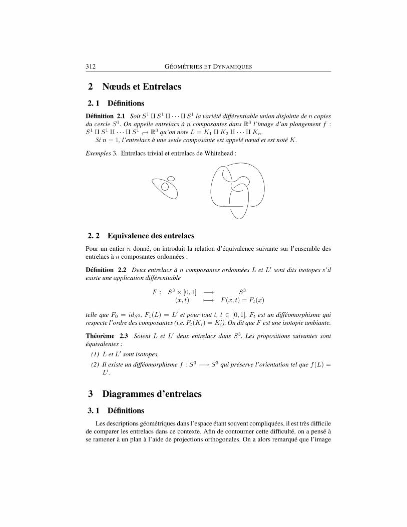
312 GEOMETRIES ET DYNAMIQUES
2 Nœuds et Entrelacs
2. 1 DefinitionsDefinition 2.1 Soit S1 qS1 q · · · qS1 la variete differentiable union disjointe de n copiesdu cercle S1. On appelle entrelacs a n composantes dans R3 l’image d’un plongement f :S1 q S1 q · · · q S1 → R3 qu’on note L = K1 qK2 q · · · qKn.
Si n = 1, l’entrelacs a une seule composante est appele nœud et est note K.
Exemples 3. Entrelacs trivial et entrelacs de Whitehead :
2. 2 Equivalence des entrelacsPour un entier n donne, on introduit la relation d’equivalence suivante sur l’ensemble desentrelacs a n composantes ordonnees :
Definition 2.2 Deux entrelacs a n composantes ordonnees L et L′ sont dits isotopes s’ilexiste une application differentiable
F : S3 × [0, 1] −→ S3
(x, t) 7−→ F (x, t) = Ft(x)
telle que F0 = idS3 , F1(L) = L′ et pour tout t, t ∈ [0, 1], Ft est un diffeomorphisme quirespecte l’ordre des composantes (i.e. Ft(Ki) = K ′i). On dit que F est une isotopie ambiante.
Theoreme 2.3 Soient L et L′ deux entrelacs dans S3. Les propositions suivantes sontequivalentes :
(1) L et L′ sont isotopes,
(2) Il existe un diffeomorphisme f : S3 −→ S3 qui preserve l’orientation tel que f(L) =L′.
3 Diagrammes d’entrelacs
3. 1 DefinitionsLes descriptions geometriques dans l’espace etant souvent compliquees, il est tres difficile
de comparer les entrelacs dans ce contexte. Afin de contourner cette difficulte, on a pense ase ramener a un plan a l’aide de projections orthogonales. On a alors remarque que l’image

H. ABCHIR 313
d’un entrelacs par une projection orthogonale particuliere sur un plan comporte toutes lesinformations necessaires pour le reconstituer dans l’espace. Dans ce qui suit, on montreraque pour comparer les entrelacs il suffit de comparer leurs projections.
Soit π une projection de l’espace sur le plan R2. Soit L un entrelacs. Un point P ∈π(L) ⊂ R2 dont l’image reciproque π−1(P ) comporte plus d’un antecedent est appele pointmultiple.
Definition 3.1 Soit π la projection orthogonale de R3 sur un plan P. On dit que π estreguliere si pour tout entrelacs L ∈ R3 :
(1) Toute droite tangente a L en un point P se projette sur une droite du plan (pas dedegeneressence).
(2) Les seuls points multiples sont les points doubles. Un point double est appele croise-ment.
(3) L’ensemble des croisements est fini et en chaque croisement les projections des lignestangentes aux points antecedents ne sont pas colineaires.
Remarque. Dans le contexte de la definition precedente, les cas de la figure 1 ne sont pasautorises.
FIG. 1 – Deux projections interdites
Definition 3.2 (diagramme) On appelle diagramme d’un entrelacs, son image par uneprojection reguliere dans laquelle on insere les informations dessus-dessous relatives auxcroisements (altitude).
3. 2 Equivalence des diagrammes
Soit L un diagramme d’entrelacs et K une composante de L. Soient P et Q deux pointssur K et l ⊂ K l’arc joignant P a Q. On considere un nouvel arc l′ reliant P a Q isotopea l tel qu’il existe une surface δ de bord l ∪ l′ verifiant δ ∩ L = l. On appelle mouvementelementaire sur L le remplacement de l par l′ ou l’operation inverse. Le nouveau diagrammeL′ est dit obtenu (apres lissage de la courbe) a partir de L par un mouvement elementaire.
On appelle une suite finie de tels mouvements isotopie plane (figure 2).

314 GEOMETRIES ET DYNAMIQUES
FIG. 2 – Isotopie plane
Remarque. Au cours d’une isotopie plane les phenomenes suivants ne doivent pas se pro-duire :
(1) l’apparition ou la disparition d’un croisement.(2) Les projections de deux branches de l’entrelacs deviennent tangentes.(3) Les points de trois branches de l’entrelacs sont projetees sur le meme point.
Cependant, les situations ci-dessus prohibees dans le plan sont les projections regulieresd’isotopies ambiantes dans l’espace. Ces projections correspondent aux mouvements suivantsdits de Reidemeister :
Ω3
Ω1 Ω2
FIG. 3 – Mouvements de Reidemeister
Definition 3.3 Deux diagrammes d’entrelacs sont dits equivalents si on peut transformerl’un en l’autre par une suite finie de mouvements de Reidemeister et d’isotopies planes.
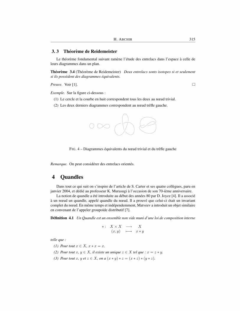
H. ABCHIR 315
3. 3 Theoreme de ReidemeisterLe theoreme fondamental suivant ramene l’etude des entrelacs dans l’espace a celle de
leurs diagrammes dans un plan.
Theoreme 3.4 (Theoreme de Reidemeister) Deux entrelacs sonts isotopes si et seulementsi ils possedent des diagrammes equivalents.
Preuve. Voir [1].
Exemple. Sur la figure ci-dessous :
(1) Le cercle et la courbe en huit correspondent tous les deux au nœud trivial.
(2) Les deux derniers diagrammes correspondent au nœud trefle gauche.
FIG. 4 – Diagrammes equivalents du nœud trivial et du trefle gauche
Remarque. On peut considerer des entrelacs orientes.
4 QuandlesDans tout ce qui suit on s’inspire de l’article de S. Carter et ses quatre collegues, paru en
janvier 2004, et dedie au professeur K. Murasugi a l’occasion de son 70-ieme anniversaire.La notion de quandle a ete introduite au debut des annees 80 par D. Joyce [4]. Il a associe
a un nœud un quandle, appele quandle du nœud. Il a prouve que celui-ci etait un invariantcomplet du nœud. En meme temps et independemment, Matveev a introduit un objet similaireen convenant de l’appeler groupoıde distributif [7].
Definition 4.1 Un Quandle est un ensemble non vide muni d’une loi de composition interne
∗ : X ×X −→ X(x, y) 7−→ x ∗ y
telle que :
(1) Pour tout x ∈ X , x ∗ x = x.
(2) Pour tout x, y ∈ X , il existe un unique z ∈ X tel que : x = z ∗ y.
(3) Pour tout x, y et z ∈ X , on a (x ∗ y) ∗ z = (x ∗ z) ∗ (y ∗ z).

316 GEOMETRIES ET DYNAMIQUES
Exemples. (1) Soit G un groupe. On prend X = G et pour x, y ∈ X ,
x ∗ y = y−n ∗ x ∗ yn
(2) Quandle Dihedral : On prend X = Zn = 0, 1, · · · , n− 1 muni de l’operation
x ∗ y = 2y − x (mod n)
(3) Soit S4 = 0, 1, 2, 3 avec les relations :
0 = 0 ∗ 0 = 1 ∗ 2 = 2 ∗ 3 = 3 ∗ 11 = 0 ∗ 3 = 1 ∗ 1 = 2 ∗ 0 = 3 ∗ 22 = 0 ∗ 1 = 1 ∗ 3 = 2 ∗ 2 = 3 ∗ 03 = 0 ∗ 2 = 1 ∗ 0 = 2 ∗ 1 = 3 ∗ 3
(4) Soit Λ = Z[t, t−1] l’anneau des polynomes de Laurent a coefficients entiers. Alors toutΛ-module M a une structure de quandle definie par a ? b = ta + (1 − t)b pour a et bdans M .Si P (t) est un polynome de Laurent dont les coefficients dominant et constant sontegaux a ±1, alors Zn[t, t−1]/(P (t)) est un quandle fini appele (mod n)-quandled’Alexander. En particulier on peut verifier que S4 ' Z2[t, t−1]/(t2 + t+ 1).
Definition 4.2 Soit f : X −→ Y une application d’un quandle X dans un quandle Y . Ondit que f est un morphisme de quandles si pour tout x, y ∈ X on a :
f(x ∗ y) = f(x) ∗ f(y)
Avant de passer au paragraphe suivant, il est interessant de noter que l’introduction dela structure de quandle a ete en partie motivee par les mouvements de Reidemeister sur lesdiagrammes d’entrelacs.
5 Cohomologie des QuandlesSoit X un quandle.On note CRn (X) le groupe abelien libre engendre par les n-uplets (x1, · · · , xn), ou xi ∈
X .Soit l’homomorphisme
∂n : CRn (X) −→ CRn−1(X)(x1, · · · , xn) 7−→ ∂n(x1, · · · , xn)
defini par
∂n(x1, · · · , xn) =n∑i=2
(−1)i[(x1, · · ·xi−1, xi+1, · · · , xn)
− (x1 ∗ xi, x2 ∗ xi, · · ·xi−1 ∗ xi, xi+1, · · · , xn)]

H. ABCHIR 317
pour n ≥ 2 et ∂0 = ∂1 = 0.On obtient ainsi le complexe de chaınes CR∗ (X) = CRn (X), ∂n.
On pose CD0 (X) = CD1 (X) = 0. Si n ≥ 2, on considere CDn (X) ⊂ CRn (X), ou CDn (X)est le sous groupe engendre par les n-uplets (x1, · · · , xn) verifiant xi = xi+1 pour un certainindice i, 1 ≤ i ≤ n− 1.
Alors CD∗ (X) = CDn (X), ∂n est un sous complexe de CRn (X), ∂n.On pose alors
CQn (X) = CRn (X)/CDn (X)
On appelle complexe de chaines du quandle X , le complexe CQ∗ (X) = CQn (X), ∂′n, ou ∂′
est l’homomorphisme induit par ∂n.Pour tout groupe abelien A, on definit les complexes de chaınes et de cochaınes suivants :
CQ∗ (X;A) = CQ∗ (X)⊗A ; ∂ = ∂ ⊗ id
C∗Q(X;A) = Hom(CQ∗ (X);A) ; δ = Hom(∂, id)
Definition 5.1 On appelle n-ieme groupe de cohomologie du quandle X le groupe
Hn(X;A) = (Hn(C∗Q(X;A))
Hn(X;A) = Zn(X;A)/Bn(X;A)
ou Zn(X;A) designe l’ensemble des cocycles et Bn(X;A) designe l’ensemble des cobords.
Remarque. Soit un 2-cocycle ϕ, ϕ ∈ Zn(X) ⊂ C2Q(X) = Hom(CQ2 (X); Z). On a :
δ2ϕ(x, y, z) = ϕ ∂3(x, y, z) = ϕ(x, z)− ϕ(x ∗ y, z)− ϕ(x, y) + ϕ(x ∗ z, y ∗ z) = 0
D’ou la relation :
ϕ(x, z) + ϕ(x ∗ z, y ∗ z) = ϕ(x, y) + ϕ(x ∗ y, z)
6 Cocycles invariants des nœudsDorenavant X designe un quandle fini fixe et A est un groupe abelien fixe note multipli-
cativement.
Definition 6.1 Soit D un diagramme oriente d’un nœud K. Soit R l’ensemble des arcs deD. On appelle coloration de D toute application
C : R −→ Xα 7−→ C(α) = x
qui verifie, en tout croisement τ de D, la propriete suivante :si α est l’arc passant au dessus en τ , et si β1 et β2 designent les sous arcs en τ tels quela normale a α pointe de β1 vers β2 alors :
C(β2) = C(β1) ∗ C(α)

318 GEOMETRIES ET DYNAMIQUES
y
x
x ∗ y
FIG. 5 – Convention de coloration
On dit que C(α) est la couleur de l’arc α.
Remarque. : En un croisement, les colorations ne dependent pas des orientations des sousarcs.
Convention des signes des croisements : On oriente le plan dans le sens contraire des ai-guilles d’une montre.
En chaque croisement, on considere la paire (N,n), ou N (respectivement n) designeun vecteur normal a l’arc dessus (respectivement dessous) oriente selon la regle de la maindroite.
Si (N,n) coıncide avec l’orientation du plan (sens inverse des aiguilles d’une montre),on dit que le croisement τ est positif. Il est dit negatif dans le cas contraire.
Definition 6.2 – Soit ϕ ∈ Z2(X;A) un 2-cocycle.– Soit D un diagramme d’un nœud oriente.– Soit C une coloration de D.– Soit τ un croisement de D. On note α,β1 et β2 respectivement l’arc passant au dessus
en τ , les sous arcs en τ tels que la normale a α pointe de β1 vers β2.– On note x = C(β1) et y = C(α).On appelle poids de C en τ associe a ϕ l’element suivant de A :
B(τ, C) := ϕ(x, y)ε(τ)
ou ε(τ) = ±1 selon que le signe de τ est positif ou negatif.
Definition 6.3 Soit ϕ ∈ Z2(X;A) un 2-cocycle. Soit D un diagramme d’un nœud K. Onappelle fonction de partition de K associee a ϕ l’expression∑
C
∏τ
B(τ, C) ∈ Z[A]
ou le produit porte sur tous les croisements deD et la somme porte sur toutes ses colorations.On l’appelle aussi somme d’etats du nœud.
Theoreme 6.4 Soit ϕ ∈ Z2(X;A) un 2-cocycle. Soit D un diagramme d’un nœud K.Alors, la fonction de partition de K associee a ϕ est independante du diagramme D choisi.Elle definit alors un invariant du nœud note Φϕ(K).
H. ABCHIR 319
Preuve. Tout d’abord on remarque qu’il y a une correspondance biunivoque entre les colora-tions avant et apres un mouvement de Reidemeister. Il suffit alors de verifier que
∏τ B(τ, C)
reste inchange par les mouvements de Reidemeister pour chaque coloration.Mouvement Ω1 :
ϕ ∈ C2(X;A) = Hom(C2(X;A).C2(X) = CR2 (X)/CD2 (X). Or (x, x) ∈ CD2 (X) et par suite il est nul dans C2(X). Commeϕ est un morphisme de groupes, ϕ(x, x) = 1 ∈ A.Mouvement Ω2 :On a la relation x ∗ y = x ∗ z, d’ou d’apres l’axiome 2 d’un quandle x = z. Ainsi les deuxtermes qui apparaissent dans le produit, ϕ(x, y) et ϕ(z, y)−1 s’eliminent mutuellement.Mouvement Ω3 :La remarque de la page 318 montre que
ϕ(x, y)ϕ(y, z)ϕ(x ∗ y, z) = ϕ(y, z)ϕ(x, z)ϕ(x ∗ z, y ∗ z)
Theoreme 6.5 L’invariant Φϕ(K) est independant de la classe de cohomologie du 2-cocycle ϕ.
En particulier, si ϕ est un cobord, la somme des etats est egale au nombre de colorationsd’un diagramme d’un nœud donne.
Preuve. Soit C une coloration fixee. On se propose de calculer∏τ B(τ, C) dans le cas ou le
2-cocycle ϕ ∈ Z2(X;A) est un cobord. Soit alors ψ ∈ C1(X;A) tel que ϕ = δψ ou δ estl’operateur cobord. Il s’en suit que pour tout (x, y) ∈ X2,
ϕ(x, y) = ψ(x)ψ(x ? y)−1
On convient d’attribuer le poids ψ(x) a l’extremite du sous arc arrivant a τ et le poids ψ(x ?y)−1 a l’extremite du sous arc partant de τ . On remarque alors que puisqu’a chaque arcest atribuee une unique couleur, les deux poids attribues aux deux extremites d’un arc sontinverses l’un de l’autre et s’eliminent ainsi mutuellement dans le produit des poids qui vautalors 1.
7 Exemples de groupes de cohomologie des quandlesOn suppose que A est un groupe cyclique note additivement : Z ou Zn.Pour tout x ∈ Xn, on definit la fonction caracteristique χx : Cn(X) −→ A telle que :
χx(y) =
1 si x = y0 si x 6= y
Alors pour toute cochaıne f ∈ CnR(X;A), on a :
f =∑x∈Xn
Cxχx

320 GEOMETRIES ET DYNAMIQUES
et si f ∈ CnQ(X;A), alors :
f =∑
x∈Xn\S
Cxχx
ou S = (x1, · · · , xn) | xj = xj+1 pour un certain j, 1 ≤ j ≤ n− 1.
Lemme 7.1H2(R3; Z) ' 0
H2(R4; Z) ' Z× ZH2(S4; Z2) = Z2
Preuve. Voir dans le paragraphe 6 de [2]
On rappelle que S4 ' Z2[t, t−1]/(t2 + t+ 1). On considere le 2-cocycle
ϕ = tχ(0,1)+χ(1,0)+χ(1+t,0)+χ(0,1+t)+χ(1,1+t)+χ(1+t,1) ∈ Z2(S4; Z2)
Theoreme 7.2 Les invariants somme d’etats du trefle et du nœud huit associes au 2-cocycleϕ defini ci-dessus sont egaux a
4 + 12t
Preuve. Chacun de ces deux nœuds peut etre colorie de 16 manieres en utilisant le quandleS4 introduit dans la page 316.
Considerons le cas du trefle droit Td represente par un diagramme D comportant troiscroisements tous positifs. Pour chaque coloration C donnee, on calcule
∏3i=1B(τi, C), ou τi
est le i-eme croisement de D. Si xi, yi et zi = xi ? yi sont les couleurs en τi, alors :
3∏i
B(τi, C) =3∏i=1
ϕ(xi, yi)
=3∏i=1
t[χ(0,1)+χ(1,0)+χ(1+t,0)+χ(0,1+t)+χ(1,1+t)+χ(1+t,1)](xi,yi)
En ecrivant ce produit pour toutes les colorations possibles de D, puis en faisant la sommedes produits obtenus, on a le resultat annonce.
8 Questions– Dans le cas ou le quandle est un groupe G avec comme loi la conjugaison, comparer la
cohomologie du quandle a celle du groupe G.– Developper des outils de calculs de la cohomologie des quandles tels que les suites
spectrales.– Preciser le comportement des fonctions de partition vis a vis des operations sur les
nœuds telle que la somme connexe.
Remerciements : Je n’oublierai pas de remercier les organisateurs de l’ecole CIMPA d’ElOued et les feliciter pour la reussite eclatante de cette manifestation scientifique.

H. ABCHIR 321
xiyi
τi
xi ∗ yi
FIG. 6 – Coloration C du Trefle en un croisement τi
Bibliographie[1] Burde et Zieschang, Knots, De Gruyter Studies in Mathematics 5.
[2] J. Scott Carter, D. Jelsovsky, S. Kamada, L. Langford and M. Saito, Quandle Coho-mology and State-Sum Invariants of Knotted Curves and Surfaces, Trans. Amer. Math.Soc. 335 (2003), 3947-3989.
[3] V.F.R Jones, Hecke algebra representations of braid groups and link polynomials, Ann.of Math. 126(1987), 335-388.
[4] D. Joyce, A classifying invariant of knots, the knot quandle, J. Pure Appl. Alg. 23(1982)37-65.
[5] R. Kirby, A calculus for framed links in S3, Invent. Math. 45(1978) 35-56.
[6] WBR Lickorish, Introduction to knot theory, Springer, GTM 175.
[7] S. Matveev, Distributive groupoids in knot theory, (Russian) Mat. Sb.(N.S.)119(161)(1982) 78-88, 160.
[8] Murasugi, Knot theory and its applications, Birkhauser.
Hamid AbchirUniversite Hassan II, Ecole superieure de TechnologieRoute d’El Jadida. B.P. 8012. Oasis. 20100 Casablanca. Maroce-mail : [email protected]


Pseudo-Parallel submanifolds
by
MOHAMED BELKHELFA
ABSTRACT. Pseudo-parallel (shortly PP) submanifolds are defined as a gen-eralization of semi-parallel (shortly SP ) submanifolds and as extrinsic analogueof pseudo-symmetric (shortly PS) manifolds (in the sense of R. Deszcz) [1], [26].Asperti et al [1] obtained a description of PP hypersurfaces in space form as quasi-umbilic hypersurfaces or cyclids of Dupin and studied PP surfaces with maximalfirst normal bundle in space form and classified complete simply connected PPsubmanifolds in space. In the last years many results obtained about a class ofsurfaces in Euclidean space, pseudo-parallel hypersurfaces in pseudo-Riemannianspace forms and pseudo-parallel real hypersurfaces in complex space forms, ap-peared in [19], [15], [16] respectively. In this paper we study the PP hypersurfacesin Riemannian manifold not necessarily a space form; Moreover we give a descrip-tion of semi-parallel surfaces in BCV spaces.
Mathematics Subject classification: 53C40 53C35.Keywords: Submanifold, symmetry, semi-symmetry, paseudo-symmetry, parallel, semi-
parallel, pseudo-parallel.Acknowledgment The author thanks the organizing committee for the invitation, hospital-
ity and generosity.
1 IntroductionLet (M, g) be a n-dimensional, n ≥ 3, semi-Riemannian connected manifold of class C∞.We denote by ∇, S, and κ the Levi-Civita connection, the Ricci tensor, and the scalar cur-vature of (M, g), respectively. A (0, k)-tensor field T on (M, g) is called parallel when it isinvariant under parallel translation, i.e. when
∇T = 0,
323
324 GEOMETRIES ET DYNAMIQUES
in particular, if the (0, 4)-Riemann-Christoffel curvature tensor R is parallel, i.e.
∇R = 0,
then M is said to be locally symmetric.In the following, by R we will also denote the curvature operator such that:
R(X,Y )Z = ∇X∇Y Z −∇Y∇XZ −∇[X,Y ]Z,
As is well known, every (1, 1)-tensor field A on a differential manifold determines aderivation A· of the tensor algebra on this manifold, commuting with contractions. In par-ticular, the anti-symmetric (1, 1)-tensor field R(X,Y ) induces derivations R(X,Y )·, thusassociating with a (0, k)-tensor field T, the (0, 2 + k)-tensor R · T defined by:
(R · T )(X1, X2, . . . , Xk;X,Y ) = (R(X,Y ) · T )(X1, X2, . . . , Xk)= −T (R(X,Y )X1, X2, . . . , Xk)− · · ·−T (X1, X2, . . . , R(X,Y )Xk).
One hasR(X,Y ) · T = ∇X(∇Y T )−∇Y (∇XT )−∇[X,Y ]T.
ByR ·R we denote in this way the (0, 6) -tensor field obtained by the derivation of the secondR, the (0, 4)- curvature tensor, using the curvature operator, the first R. If
R ·R = 0, (1)
then M is called a semi-symmetric space [20], [22]. It was already recognized by E. Cartanthat all locally symmetric spaces and all 2-dimensional Riemannian space fulfill the condi-tion (1). When talking about semi-symmetry, we will always assume n ≥ 3. The condition ofsemi-symmetry for hypersurfaces M of Euclidean spaces En+1 was first studied by K. No-mizu in [18]. He asked the question if there exist complete irreducible and simply connectedRiemannian manifolds of dimension n ≥ 3 satisfying R · R = 0 and which are not locallysymmetric. In 1972, R. Takagi [24] and later also K. Sekigawa produced such examples, ashypersurfaces in Euclidean spaces. In 1982-84 Z. Szabo obtained a full intrinsic classifica-tion of semi-symmetric Riemannian manifolds. And soon after that Z. Szabo and J. Deprez,independently, obtained the classification of all semi-symmetric hypersurfaces in Euclideanspaces [9], [21].
Locally, each semi-symmetric space belongs to one of the following three classes:
(1) the trivial class consisting of all locally symmetric spaces and all 2-dimensional Rie-mannian manifolds,
(2) the exceptional class of all elliptic, hyperbolic, Euclidean and Kahlerian cones,
(3) the typical class of all Riemannian manifolds foliated by Euclidean leaves of codimen-sion two [20], [22].

M. BELKHELFA 325
2 Pseudo-symmetryTo state the definition of pseudo-symmetry in Deszcz sense, we first determine a (0, k + 2)-tensor Q(g, T ) associated with any (0, k)- tensor field T on a semi-Riemannian manifold Mby:
Q(g, T )(X1, X2, . . . , Xk;X,Y ) = ((X ∧g Y ) · T ) (X1, X2, .., Xk)= −T ((X ∧g Y )X1, X2, .., Xk)−−T (X1, X2, . . . , Xk−1, (X ∧g Y )Xk)),
where X ∧g Y denotes the endomorphism given by:
X ∧g Y = g(Y, Z)X − g(X,Z)Y.
A semi-Riemannian manifold Mn = (Mn, g), n ≥ 3, is said to be pseudo-symmetric in thesense of R. Deszcz if the (0, 6)-tensor fields R ·R and Q(g,R) on M are linearly dependent,i.e., if there exists a function
LR : M −→ R
such thatR ·R = LRQ(g,R) (2)
holds on UR = x ∈ M |R − κn(n−1)G 6= 0 at x, where G is the (0, 4)-tensor of (M, g)
defined byG(X1, X2, X3, X4) = g((X1 ∧g X2)X3, X4)
for all X1, X2, X3, X4 vector fields of M [3], [10], [26].Clearly, every semi-symmetric manifolds is pseudo-symmetric. The converse is not true;there are pseudo-symmetric manifolds which are not semi-symmetric. For instance, thewarped product Sp ×F Sn−p, p ≥ 2, n − p ≥ 1, of the standard spheres Sp and Sn−p withsome warping function F and Schwarzschild space time are a non semi-symmetric pseudo-symmetric manifold [10]. We mention also that certain spacetimes are pseudo-symmetric,among others: the Robertson-Walker spacetimes and generalized Robertson-Walker space-times, the Kottler spacetimes as well as the Riessner-Nordstrom spacetimes [7], [11]. Thecondition of pseudo-symmetry arose during the study of totally umbilical submanifolds ofsemi-symmetric manifolds, and also arose during the consideration of geodesic mapping ontosemi-symmetric manifolds [3], [10], [26].It is known that every totally umbilical submanifold, with parallel mean curvature vectorfield is also pseudo-symmetric (or more generally, in a pseudo-symmetric) manifold is alsopseudo-symmetric. In particulair, extrinsic spheres in pseudo-symmetricRiemannian man-ifold are also pseudo-symmetric. Further, if a semi-Riemannian manifold (M, g)admits ageodesic mapping (A diffeomorphism which maps geodesic lines into geodesic lines) onto asemi-symmetric (or more generally, in a pseudo-symmetric) manifold then (M, g) is pseudo-symmetric.
Remark 2.1. [10]Q(g,R) = 0⇐⇒ R =
κ
n(n− 1)G

326 GEOMETRIES ET DYNAMIQUES
If at a point x ∈M , we have R = κn(n−1)G then R ·R = 0 holds at x. Thus the pseudosym-
metry condition is trivially fulfilled on M − URA hypersurface M of En+1 is pseudo-symmetric if and only if M is semi-symmetric or
has at most two distinct principal curvatures [10], [26].
3 Extrinsic notions of pseudo-symmetry
Let M be a submanifold of Riemannian manifold N , when N is a space form (i.e. Withconstant sectional curvature c) will be denote by N(c) and let h be the second fundamentalform of M .
The extrinsic analogous classes of symmetric, semi-symmetric and pseudo-symmetricrespectively are: symmetric or parallel submanifold (∇h = 0), semi-parallel submanifold(R · h = 0) and pseudo-parallel submanifold (R · h = LhQ(g, h)). For parallel and semi-parallel submanifolds and others generalizations see [17].
The basic Gauss, Codazzi-Mainardi and Ricci equations give that the extrinsic condi-tions Parallel, semi-parallel and pseudo-parallel imply the correspondent intrinsic conditionssymmetry, semi-symmetry and pseudo-symmetry respectively see [1]
Proposition 3.1 Let Mn be a hypersurface of Riemannian manifold (Nn+1, g) and let ξ aunit normal vector and e1, e2, . . . , en be an orthonormal basis of the tangent space of Mn
which diagonalizes the Weingarten operator Aξ. If Mn is pseudo-parallel then:
[K(ei, ej) + λiλj − Lh](λj − λi) = 0, (3)
for all i 6= j
Where λi = g(Aξei, ei), K(ei, ej) = g(R(ei, ej)ej , ei) and R is the Riemannian curva-ture of Nn+1
Proof. Let λi = g(Aξei, ei) be the principal curvature in the direction of ξ, following theproof in [1] and using the Gauss equation we get the equation 3
Corollary 3.2 If (Nn+1, g) is a space form with constant curvature c and Mn is PP we get
[c+ λiλj − Lh](λj − λi) = 0, (4)
for all i 6= j
Which is the proposition 3.1 [1] up sign in the second term, because they used the wedgeproduct (X ∧g Y )Z = g(X,Z)Y − g(Y,Z)X.
Remark 3.1. The work is in progress for the hypersurface in Sasakian space form.
The condition 3 is also sufficient for PP.
Remark 3.2. For n = 2. Lh is the Gauss curvature; So every surface is PP. Which is not thecase for SP surfaces.

M. BELKHELFA 327
In [4] We classified parallel surfaces in BCV spaces. The following 2-parameter familyof Riemannian metrics.
gl,m =dx2 + dy2
1 +m(x2 + y2)2+(dz +
l
2ydx− xdy
1 +m(x2 + y2)
)2
, l, m ∈ R. (5)
is called the Bianchi-Cartan-Vranceanu metrics. The metrics as above are defined over thewhole 3-space R3 for m ≥ 0 and over the region x2 + y2 < −1/m for m < 0. We shall callthe homogeneous Riemannian 3-manifolds M3 = (M3, gl,m) defined by
M3 =((x, y, z) ∈ R3 | 1 +m(x2 + y2) > 0, gl,m
)the Bianchi-Cartan-Vranceanu spaces (BCV-spaces in short)[4].
Theorem 3.3 [4] Let (M3, gl,m) be the BCV-space with 4m− l2 6= 0.
(1) If l 6= 0 : then the only parallel surfaces in (M3, gl,m) are Hopf cylinders over Rie-mannian circles in M2.
(2) If l = 0 : then the only parallel surfaces in Riemannian symmetric space M30,m with
m 6= 0 are totally geodesic leaves and Hopf cylinders over Riemannian circles in M2.
Here Riemannian circles in M2 are curves in M2 with constant geodesic curvature, where
M2 =((x, y) ∈ R2 | 1 +m(x2 + y2) > 0 , dx2 + dy2
1 +m(x2 + y2)2
).
Let γ be a curve parametrised by arclength in M3/ξ with curvature κ. Then taking theinverse image S := π−1(γ) of γ in M3. We shall call this surface S the Hopf cylinder (orBoothby-Wang cylinder) over γ, where ξ = ∂
∂z .Take an orthonormal frame field E = (e1, e2, e3):
e1 = 1 +m(x2 + y2) ∂∂x− ly
2∂
∂z, e2 = 1 +m(x2 + y2) ∂
∂y+lx
2∂
∂z,
e3 =∂
∂z.
Then the dual coframe field ϑ = (θ1, θ2, θ3) is given by
θ1 =dx
1 +m(x2 + y2), θ2 =
dy
1 +m(x2 + y2), θ3 = dz +
λ
2ydx− xdy
1 +m(x2 + y2).
Note that the one-form η := θ3 is a contact form on M3 if and only if l 6= 0. The Levi-Civitaconnection ∇ of M is described by the formulae:
∇e1e1 = 2mye2, ∇e1e2 = −2mye1 +l
2e3, ∇e1e3 = − l
2e2,
∇e2e1 = −2mxe2 −l
2e3, ∇e2e2 = 2mxe1, ∇e2e3 =
l
2e1, (6)

328 GEOMETRIES ET DYNAMIQUES
∇e3e1 = − l2e2, ∇e3e2 =
l
2e1, ∇e3e3 = 0.
[e1, e2] = −2mye1 + 2mxe2 + le3, [e2, e3] = [e3, e1] = 0. (7)
the curvature tensor R is described by the formula:
R1212 = 4m− 34l2, R1313 = R2323 =
l2
4. (8)
The Ricci tensor Ric of M is given by
R11 = R22 = 4m− l2, R33 =l2
2.
Hence the scalar curvature s is s = 8m− l2/2.
Remark 3.3. The geodesics of M3 are calculated by Sitzia [23], see also [5], [2], for geo-metric properties of this metric.
Proof. Let X1, X2, X3 be an orthonormal frame field of S such that X3 = N . Denote byω1, ω2, ω3 the dual coframe field to Xi. We can write ω3 = pθ1 + qθ2 + rθ3. Sinceωi is orthonormal, p2 + q2 + r2 = 1. The vector fields u1 = re1 − pe3, u2 = re2 − qe3
are tangent to S. In particular if r 6= 0, u1, u2 is a (local) frame field on S. By directcomputations using (3.4) we obtain the following:
Lemma 3.4 The normal components of curvature tensor R are described by
(R(u1, u2)u1)⊥ = qr3(l2 − 4m)N, (R(u1, u2)u1)⊥ = −pr3(l2 − 4m)N.
Assume that the second fundamental form h of S is parallel. Then the Codazzi equationimplies:
(R(u1, u2)u1)⊥ = (∇u1h)(u2, u1)− (∇u1h)(u1, u1) = 0. (9)
Similarly we have(R(u2, u1)u2)⊥ = 0. (10)
First we consider the case r 6= 0.Case I r 6= 0.The preceding lemma implies p = q = 0, since we assumed λ2 − 4µ 6= 0. Hence
ω3 = θ3. Namely S is an integral surface of the distribution D defined by η = 0.
Subcase (i) l = 0: in this case S is an integral surface of the distribution D definedby dz = 0. Hence S is a leaf M2 × z0 for some z0. Note that this leaf is totallygeodesic.
Subcase (ii) l 6= 0: since η in this case is a contact form, there are no integral surfacesof D. This implies that this case cannot occur.

M. BELKHELFA 329
Case II r = 0.In this case ω3 has the form ω3 = pθ1 + qθ2. Since p2 + q2 = 1, we may write
p = cosϕ, q = sinϕ. In addition, the orthonormal vector fields v1 = qe1 − pe2, v2 = e3
give an orthonormal frame field tangent to S.Next by using (3.4), we have
∇v1v1 = v1(q)e1 − v1(p)e2 + 2m(px+ qy)N, ∇v1v2 = − l2N,
∇v2v1 = − l2N + (v2(q)e1 − v2(p)e2), ∇v2v2 = 0.
By the symmetry of second fundamental form, we get pv2(q)−qv2(p) = 0. Equivalentlywe have v2(ϕ) = 0.
By the Gauss formula we obtain the induced connection and the second fundamentalform:
∇v1v1 = 0, ∇v1v2 = 0, ∇v2v2 = 0, (11)
h(v1, v1) = v1(ϕ) + 2m(px+ qy)N, h(v1, v2) = − l2N, h(v2, v2) = 0. (12)
The mean curvature vector field H of S defined by
H =12
tr h (13)
is computed asH = HN, 2H = v1(ϕ) + 2m(px+ qy).
Since h is parallel, the mean curvatureH is constant. Furthermore (3.9) implies that S is flat.Moreover (3.9) implies that we can take z as a (local) coordinate of S and hence there existsa local coordinate system (t, z) such that
∂
∂t= v1.
Thus the equation v2(ϕ) = 0 implies that ϕ depends only on t. With respect to this coordinatesystem (t, z), the constancy of H is rewritten as
dϕ
dt= 2H −m(cosϕ(t)x(t) + sinϕ(t)y(t)), H ∈ R. (14)
It is easy to see that S is generated by two coordinate curves. The z-coordinate curves aregeodesics and integral curves of the vector field e3. The t-coordinate curves are horizontalcurves of curvature 2H . Let us denote by γ(t) the t-coordinate curve in M3. Then it is easyto see that γ is a Frenet curve of osculating order at most 3. The principal normal vector fieldof γ is the restriction of N on γ. The binormal vector field B of γ is ±e3. We can assumeB = e3. The Frenet-Serret formulas of γ are given by
∇γ′(T,N,B) = (T,N,B)
0 −2H 02H 0 − l
2
0 l2 0
(15)
330 GEOMETRIES ET DYNAMIQUES
This implies that t-coordinate curves are of constant torsion l/2. Hence t-coordinate curvesare horizontal curves of curvature 2H . Let us denote by γ(t) = (x(t), y(t)) the projectionof γ to M2, namely γ = π γ. One can check that γ(t) is of constant curvature 2H .Equivalently t-coordinate curves are horizontal lifts of Riemannian circles of curvature 2Hin M2. (In particular the case H = 0, γ is a geodesic in M2.)
Recall the surface S is parameterized by t and z. And the t-coordinate curves are hor-izontal lifts of Riemannian circles in the base space with curvature 2H . Thus we concludethat S is a Hopf cylinder over a Riemannian circle of curvature 2H . In particular, S is pa-rameterized by (x(t), y(t), z). We finish this paper by considering these Riemannian circlesmore in detail.
From the definition of v1, we notice that
dx
dt= sinϕ(t)f(t),
dy
dt= − cosϕ(t)f(t), f(t) := 1 + µ(x(t)2 + y(t)2). (16)
Here ϕ(t) is the solution to (3.12). The equation (3.14) says t is the arc length parameter ofγ.
The function f(t) satisfies the following ordinary differential equation:
d
dtlog |f(t)| = 2µx(t) sinϕ(t)− y(t) cosϕ(t). (17)
On the other hand, differentiating (3.12),
d2ϕ
dt2(t) =
dϕ
dt(t)
d
dtlog |f(t)|. (18)
If ϕ′ = 0, then from (3.14) we obtain that γ is a straight line. So we assume that ϕ′ 6= 0.Comparing (3.15) and (3.16), we have
f(t) = αϕ′(t), α ∈ R.
Hence we obtain the following explicit expression for γ:
(x(t), y(t)) = (−α cosϕ(t) + x0,−α sinϕ(t) + y0). (19)
Therefore the curve is a circle centered at (x0, y0).
Therefore it is interesting to study SP in some special manifolds, namely BCV spaces wegot
Theorem 3.5 Let M2 be a surface of Riemannian manifold (N3, gl,m) (BCV spaces) withm 6= 0 and 4m− l2 6= 0.
Then M2 is properly SP (non parallel) if and only if it is flat.
Proof. The Corollary 8.4 [4] implies the nonexistence of totally geodesic surfaces and ex-trinsic spheres–i.e., totally umbilical surfaces with parallel mean curvature vector fields, incontact 3-space forms with c 6= 1. Therefore using the corollary and suppose that the surfaceis semi-parallel we show that the surface is flat.

M. BELKHELFA 331
Example 4. [14] Let f be a linear function of x and y. Then it is easy to see that the graph rof f is a plane and is minimal in (N3, g1,0) . However planes are not flat. In fact the Gaussiancurvature is given by
K =3 + 2(b− x/2)2 + 2(a+ y/2)2
41 + 2(b− x/2)2 + (a+ y/2)22> 0
for f(x, y) = ax + by + c, a, b, c ∈ R. Which is not semi-parallel. We know that everysurface is semi-symmetric, this shows that semi-symmetric do not imply semi-parallel.
Example 5. Let (f(u), g(u)) be a regular curve parametrised by arclength in xz-plane suchthatf(u) > 0. The surface of revolution with profile curve (f(u), g(u)) = (u, 1
6
√(u2 + 3)3 is a
flat surface in (N3, g1,0) [6] then it is SP surface.
Example 6. Let (x(u), y(u)) be a curve in the xy−plane parametrised by arclength u. Thecylinder over a curve (x(u), y(u)) is M(u, v) = (x(u), y(u), v), its mean curvature is H =12x(u)y(u)− x(u)y(u) = −κ(u)
2 , where κ(u) is the curvature of the curve (x(u), y(u)),and x(u), x(u) denote the second and the first derivative respectively [4]. We remark that ifκ(u) is non constant then the cylinder in (N3, g1,0) is SP non parallel.
Remark 3.4. (1) For the geometric interpretation of Pseudo symmetry see [13]
(2) J.Van der veken proved in his PhD thesis that ”A surface immersed in an arbitrarythree-dimensional Riemannian manifold is semi-parallel if and only if it is flat or totallyumbilical.” [25].
References[1] A. C. Asperti,G. A. Lobos and F. Mercuri, Pseuo-parallel submanifols of a space form,
Adv. Geom. 2 (2002),57-71.
[2] M. Belkhelfa, R. Deszcz, and L. Verstraelen, Pseudosymmetry of 3-dimensional D’Atrispace, Dept. Math., Agricultural Univ. Wrocław, Ser. A, Theory and Methods, ReportNo. 86 (2000).
[3] M. Belkhelfa, R. Deszcz, M. Gl ogowska, M. Hotlos, D.Kowalczyk and L. Verstraelen,On some type of curvature conditions, Banach Center Publications 57 (2002) 179-194.
[4] M. Belkhelfa, F. Dillen and J. Inoguchi, Surfaces with parallel second fundamentalform in Bianchi-Cartan- Vranceanu-spaces, to Banach Center Publications 57 (2002)57-87.
[5] F. Borghero and R. Caddeo, Une structure de Separabilite et Geodesiques dans les HuitGeometries Tridimensionalles de Thurston, Rend. Mat. Appl. (7) 9, (1989), 607-624.
[6] R. Caddeo, P. Piu and A. Ratto Rotational surfaces inH3 with constant Gauss curvature,Boll. Unione Mat. Ital., VII. Ser., B 10, 2, (1996), 341-357.

332 GEOMETRIES ET DYNAMIQUES
[7] F. Defever, R. Deszcz, L. Verstraelen and L. Vrancken, On pseudo-symmetric space-times, J. Math. Phys. 35 (1994), 5908–5921.
[8] J. T. Cho and J. Inoguchi Pseudo-symmetric contact 3-manifolds, J. Korean Math. Soc.42 (2005), 913–932.
[9] J. Deprez, Semi-parallel hypersurfaces, Rend. Semin. Mat., Torino 44 (1986), 303-316.
[10] R. Deszcz, On pseudo-symmetric spaces, Bull. Soc. Math. Belg, 44 (1992), 1–34.
[11] R. Deszcz, L. Verstraelen and L. Vrancken, On the symmetry of the warped product,Gen. Relativity Gravitation, 23 (1991), 671–681.
[12] D. Ferus, Symmetric submanifolds of Euclidean space, Math. Ann, 247 (1980), 81-93.
[13] S. Haesen and L. Verstraelen, Properties of a scalar curvature invariant de- pending ontwo planes, Manuscripta Math. 122 (2007), 59-72.
[14] J. Inoguchi, T. Kumamoto, N. Ohsugi and Y. Suyama, Differential Geometry of curvesand surfaces in 3-dimensional homogeneous spaces II, Fukuoka Univ. Sci. Rep., 30(2000), 17-47.
[15] G. A. Lobos, Pseudo-parallel Hypersurfaces in pseuod-Riemannian space forms, Publ.R. Soc.Mat. Esp. 6,(2004), 229-234 . space forms, , (2004).
[16] G. A. Lobos and M. Ortegae, Pseudo-parallel real Hypersurfaces in complex spaceforms, Bull. Korean. Math. Soc, 41, No.4, (2004), 609-618.
[17] Ulo. Lumiste, Submanifolds with parallel fundamental form, in : Handbook of Differ-ential Geometry, Amsterdam: North-Holland, I ( 2000), 779-906.
[18] K. Nomizu, On hypersurfaces satisfying a certain condition on the curvature tensor,Tohoku Math. J, 20 (1968), 46-59.
[19] C. Ozgur, K. Arslan and C. Murathan, On Class of surfaces in the Euclidean space,Commun. Fac. Univ.Ank. Series A1, Vol. 51. No 1 (2002), 47-54
[20] Z.I. Szabo, Structure theorems on Riemannian spaces satisfying R(X,Y ) · R = 0, I.The local version, J. Diff. Geom. 17 (1982), 531-582.
[21] Z.I. Szabo, Classification and construction of complete hypersurfaces satisfyingR(X,Y )R = 0. Acta Sci. Math. 47 (1984), 321-348
[22] Z.I. Szabo, Structure theorems on Riemannian spaces satisfying R(X,Y ) · R = 0, II.Global versions, Geom. Dedicata 19 (1985), 65-108.
[23] P. Sitzia, Explicit formulas for geodesics of three-dimensional homogeneous manifoldswith isometry group of dimension 4 or 6, preprint, Univ. Cagliari, (1989).
[24] H. Takagi, An example of a Riemannian manifold satisfying R(X,Y ) · R = 0 but not∇R = 0, Tohoku Math. J. 24 (1972), 105-108.

M. BELKHELFA 333
[25] J. Van der veken, Submanifolds of homogeneous spaces, PhD thesis, KULeuven 2007.
[26] L. Verstraelen, Comments on pseudo-symmetry in the sense of Ryszard Deszcz, Geom-etry and Topology of Submanifolds VI, World Sci. Publ. (1994), 199-209.
Mohamed BelkhalfaLaboratoire de Physique Quantique de la Matiere et Modelisations MathematiquesCentre Universitaire de MascaraRoute de Mamounia, Mascara 29000, Algeriee-mail: [email protected], [email protected]


Area of vector fields on the sphereand related problems
by
VINCENT BORRELLI and OLGA GIL-MEDRANO1
This article is divided into two parts. The first one is an announcement of a result regard-ing unit vector fields on the 2-sphere 2 and the second one is a list of related open problems.Indeed, one of the intentions of the Ecole-CIMPA at El Oued was to provide advanced stu-dents with the opportunity to discover new areas and open problems on which they could setto work with a reasonnable hope to make significant progress. Our opinion is that the studyof volume of vector fields is such an area and that is the reason why we have included thislist of open questions.
2000 Mathematics Subject Classification : 53C20Keywords and phrases : Volume, Vector field.
1 Vector fields with least areaA vector field V on a manifold M is a section of its tangent bundle TM. If (M, g) is aRiemannian manifold, its tangent bundle is endowed with a natural Riemannian metric calledthe Sasaki metric (TM, gSas) which is defined by the following formula
∀X,Y ∈ TTM, gSas(X,Y ) = g(dπ(X), dπ(Y )) + g(K(X),K(Y ))
where π : TM −→ M is the natural projection and K : TTM −→ TM the connector ofthe Levi-Civita connection∇ of g (∇V = K dV ). It ensues that the horizontal and verticaldistributions are orthogonal, moreover the metric on each of these distributions is just the“pull-back” of g by π and K.
Suppose now that (M, g) is compact. The volume of the vector field V : M −→ TM isthe volume of the image submanifold V (M) ⊂ TM computed with the metric induced by the
1The second author is supported by Spanish DGI and FEDER (Project MTM2004-06015-C02-01) and by AVCiT(grupos03/169)
2Proofs will appear elsewhere.
335

336 GEOMETRIES ET DYNAMIQUES
Sasaki metric gSas. It is denoted by V ol(V ). Historically the first studied question regardingthe volume was the one of the infimum: given a compact, oriented Riemannian manifoldwithout boundary, is there a vector field of least volume ? To avoid the trivial answer V ≡ 0it is usually assumed that the infimum is taken among unit vector fields, that is vector fieldsV : M −→ TM such that
∀x ∈M, gx(Vx, Vx) = 1.
From now on, we will always assume that this condition holds, in particular since M has noboundary, the infimum question makes sense if and only if the Euler number χ(M) vanishes.
Since V : M → T 1M is a section, that is –roughly speaking– a graph, we have
V ol(M) ≤ V ol(V )
and a direct computation shows that equality holds if and only if the field V is parallel, i. e.∇V = 0. Therefore the problem is actually interesting when M does not admit any parallelfield. A natural example of such a situation is given by standard odd-dimensional spheresS2m+1, m ≥ 1.
The problem of finding the infimum of the volume turns out to be very difficult, even forthe usual spheres S2m+1 ! In fact the only spheres for which the problem is solved are S1 andS3. The case of S1 is straightforward since there is only two unit vector fields and both areparallel. The case of S3 is far more involved, the space of unit vector fields is homeomorphicto the space of maps from S3 to S2 and none of them is parallel. In a pionnering work,H. Gluck and W. Ziller proved, using a calibration argument, that Hopf vector fields are theunique minimizers of the volume [7] (a Hopf vector field is any vector field tangent to thefibers of a Hopf fibration S1 −→ S2m+1 −→ CPm). For the other odd-dimensional sphereswhat is known is that Hopf vector fields do not achieve the minimum [8], [5], [1]. In fact itis conjectured [8] that the infimum of the volume is achieved by singular vector fields thatwe called, Pontrjagin fields. These fields are obtained by parallel translation of a given unitvector v ∈ TpS2m+1 along geodesics radiating from the point p. The antipodal point −p issingular with index 0 = χ(S2m+1) and so can be removed, precisely, P can be approximatedby a family of non singular unit vector fields (Pε)ε∈]0,1] and such that
limε→0
V ol(Pε) = V ol(P ).
One unpleasant fact regarding the volume problem for unit vector fields is that the topo-logical condition χ(M) = 0 eliminates many interesting manifolds, almost all surfaces forinstance. Fortunately there are many ways to bypass this restriction: for example by consid-ering unit vector fields with isolated singularities or by considering a new class of unit vectorfields that we have called unit vector fields without boundary.
Definition 1.1 Let U be a dense open set of M and V : U → T 1M be a smooth vectorfield over U . The field V is said to be without boundary if the adherence V (U) of its image inT 1M is a (topological) submanifold without boundary. This submanifold is denoted by V .
It is easily seen that every Riemannian oriented manifold admits unit vector fields withoutboundary and so we can re-set the question of the infimum of the volume for this large familyof manifolds. Coming back to our spheres Sn it is obvious that Hopf vector fields have no

V. BORRELLI, O. GIL-MEDRANO 337
boundary since they are defined everywhere. For Pontrjagin fields P it turns out that they alsohave no boundary. In fact P is a submanifold without boundary which is smooth if n = 2and smooth everywhere except at a singular point if n > 2, precisely, P is homeomorphic toRPn with an RPn−2 smashed to a point [8].
Note that if P : Sn \ pt → T 1Sn is a Pontrjagin field then its restriction V = P|Uto any dense open set U of Sn \ pt is a vector field without boundary which have sameadherence and same volume. Nevertheless, strictly speaking, V is not a Pontrjagin field, thatis why it is convenient to enlarge a little bit our definition of a Pontrjagin field. We say thatV : U → T 1Sn is a Pontrjagin field in the generalized sense if V = P for a certain Pontrjaginfield P. In particular V and P coincide in a dense open set of Sn.
Theorem 1.2 Vector fields without boundary of least area on S2 are Pontrjagin fields (inthe generalized sense) and no others.
The following picture shows a Pontrjagin field on S2, its integral lines are mapped by thestereographic projection onto straight lines. Note that the index of the unique singularity ofP is 2 since χ(S2) = 2 and so the singularity can not be removed.
2 Related problemsProblem 1. Here is a question that naturally follows our theorem: what about the other com-pact orientable Riemannian surfaces of constant curvature ? The genus one case is trivialsince any flat torus T 2 = C/Λ admits parallel unit vector fields. The interesting –and mostlikely difficult– case is the one of the 2-dimensional space forms of negative Gaussian curva-ture that is genus g > 1 Riemannian surfaces which are quotients of the hyperbolic disk H2
by groups of isometries Γ acting freely and properly discontinuously on H2.There is a related problem which could be a bit easier. A fundamental result, due to
F. Brito, P. Chacon and A. Naveira [3], states that if V is a unit vector field on a compactRiemannian oriented manifold M of dimension n = 2m+ 1 then
V ol(V ) ≥∫M
(1 +
m∑i=1
CimC2i
2m
|σ2i(V ⊥)|
)dvolM

338 GEOMETRIES ET DYNAMIQUES
where σ2i(V ⊥) is the 2i-th elementary function of the second fundamental form of the distri-bution V ⊥ (which is not necessarily integrable). When m ≥ 2, equality holds if and only ifV is totally geodesic and V ⊥ integrable and umbilic. This inequality can be simplified if Mhas constant sectional curvature c, in that case there is an integral formula for the symmetricfunctions σi, precisely (see [4])∫
M
σi(V ⊥)dvolM =Cmi/2c
i/2vol(M) if i even,0 if i odd
and so the above above inequality gives a lower bound for the volume in terms of c andV ol(M). In particular, for the standard sphere M = S2m+1, it yields:
V ol(V ) ≥ V ol(R).
where R is a radial field, i. e. any unit vector field which is tangent to geodesics radiatingfrom a given point p ∈ S2m+1. This field has two singular antipodal points, the adherenceof its image in the unit tangent bundle is a submanifold with two boundary components,namely the two fibers over the singular points. Therefore R is not a unit vector field withoutboundary.
Although very important, the result of Brito, Chacon and Naveira does not solve theproblem of the infimum of the volume because there is no known globally defined family ofunit vector fields Rε of S2m+1 such that
limε→0
V ol(Rε) = V ol(R).
Note also that their result gives no information for even-dimensional manifolds, in fact,the technic used in the proof totally fails in these dimensions. An important topic will bethe search of a similar result for even-dimensional manifolds, and in particular, in the 2-dimensional case.
Problem 2. What is the influence of normalization ? Instead of choosing a unit vector field,we could also consider vector fields of constant norm, or equivalently, we could perform adilatation of the metric gk = 1
kg while keeping the length ‖V ‖gk equals to one. Of course ifV is a unit vector field for (M, g) then V k = k−
12V is a unit vector field for (M, gk) and a
direct computation shows that
V olgk(V k) =∫M
√det
(1kId+A
)dvolg
=∫M
√1kn
+1
kn−1σ1(A) + ...+
1kσn−1(A) + σn(A)dvolg
where A denotes (∇V )T ∇V and the σj are the elementary symmetric functions of theeigenvalues of A. Note that ‖V ‖g = 1 implies σn(A) = 0. If k is large, the behaviour of thevolume is ruled by the twisting of V :
Tw(V ) =∫M
√σn−1((∇V )T ∇V )dvolg.

V. BORRELLI, O. GIL-MEDRANO 339
It is shown in [1] that Hopf vector fields achieve the minimum of the twisting in odd-dimensional spheres giving an evidence that Hopf vector field could achieve the minimumof the volume for large value of k. Naturally the proof totally collapses for even-dimensionalspheres since in that case there is no Hopf vector fields... The question is to find an analogousresult on even-dimensional spheres and in particular when the dimension is 2.
If k is small, the behaviour of the volume is ruled by the energy
E(V ) =12
∫M
(n+ σ1((∇V )T ∇V )
)dvolg =
12
∫M
(n+ ‖∇V ‖2
)dvolg.
It is shown in [2] that the energy of the radial vector field is the infimum of the energy ofsmooth unit vector fields in odd-dimensional spheres. The result is based on the contructionof a family of unit vector fields Rε of S2m+1 such that
limε→0
E(Rε) = E(R).
In this construction, the fact that the dimension is odd is also crucial.
Problem 3. What is the “volume cost” of singularities ? Suppose first that V is a unit vectorfields without boundary of S2 with a unique singular point p ∈ S2 and let D2 be a small2-disk of S2 centered at p. Since the Euler number χ(S2) is 2 the index of p must also be2, hence the image V (∂D) is a closed curve that surrounds twice the fiber over p and theadherence
V (D2 \ p)
is a Moebius band µ2. It ensues that V is a Moebius band glued along its boundary to theimage V (S2 \D2) which is topologically a 2-disk, thus V is homeomorphic to RP 2. Assumenow that V has several singularities, since V is a manifold, their indexes must be 2,0 or -2.The essential singularities are the ones with indexes ±2 and from the above discussion, eachof them creates a Moebius band. So, if V has N essential singularities and if D1, ..., DN areN disjoint small disks centered at the singularities, V is homeomorphic to(
S2 \ (D1 ∪ ... ∪DN ))∪ µ2 ∪ ... ∪ µ2︸ ︷︷ ︸
N times
and so V is a connected sum of a projective space and several tori
V ' RP 2] T 2 ]...] T 2︸ ︷︷ ︸N−1
2 times
(N must be odd for obvious topological reasons).Our intuition seems to tell us that adding singularities should increase the volume since
the topology of the image actually increases with the number of singularities. In an otherhand, radial fields on S2 which have two singularities, have less volume than Pontrjaginfields with only one singularity. Whatever finding the infimum of the volume among vectorfields without boundary with exactly N essential singularities is an open problem.

340 GEOMETRIES ET DYNAMIQUES
Problem 4. A natural way to find minimizers of the volume is to look for stable criticalpoints of the volume functional (recall that a critical field V is said to be stable if the quadraticform (Hess Vol)V is non negative). In [6] it has been computed the condition that a vectorfield should fulfill in order to be critical and in [5] one can find the second variation of thefunctional at critical points. In particular, all critical vector fields on a surface are stable.
Up to now, the only examples of critical vector fields defined on an open subset of S2
are those described above: radial vector fields and Pontrjagin ones. An open question is toknow if there are other unit critical vector fields on S2. The same question of determiningall critical unit vector fiels is open for compact surfaces of constant negative curvature. Forany even-dimensional sphere the similar problem could be addressed, although in that caseit would be natural to determine first if radial and Pontrjagin are the only critical stable unitvector fields.
References
[1] V. BORRELLI AND O. GIL-MEDRANO, A critical radius for unit Hopf vector fields onspheres, to appear in Math. Ann.
[2] V. BORRELLI, F. BRITO AND O. GIL-MEDRANO, The infimum of the energy of unitvector fields on odd-dimensional spheres, Ann. Global Analysis Geom. 23 (2003), 129-140.
[3] F. BRITO, P. CHACON AND A. M. NAVEIRA, On the volume of unit vector fields onspaces of constant sectional curvature, Comment. Math. Helv. 79(2004), 300-316.
[4] F. BRITO, R. LANGEVIN AND H. ROSENBERG, Integrale de courbure sur des varietesfeuilletees, J. Diff. Geom. 16 (1981), 19-50.
[5] O. GIL-MEDRANO AND E. LLINARES-FUSTER, Second variation of Volume and En-ergy of vector fields. Stability of Hopf vector fields, Math. Ann. 320 (2001), 531-545.
[6] O. GIL-MEDRANO AND E. LLINARES-FUSTER, Minimal unit vector fields, TohokuMath. J. 54 (2002), 71-84.
[7] H. GLUCK AND W. ZILLER, On the volume of a unit vector field on the three-sphere,Comment. Math. Helv. 61 (1986), 177-192.
[8] S. L. PEDERSEN, Volumes of vector fields on spheres, Trans. Amer. Math. Soc. 336(1993), 69-78.

V. BORRELLI, O. GIL-MEDRANO 341
Vincent BorrelliInstitut Girard Desargues, Universite Claude Bernard, Lyon 143, boulevard du 11 Novembre 191869622 Villeurbanne Cedex, Francee-mail : [email protected]
Olga Gil-MedranoDepartamento de Geometrıa y Topologıa, Facultad de MatematicasUniversidad de Valencia46100 Burjassot, Valencia, Espanae-mail : [email protected]


Groupes d’homeomorphismesd’espaces metriques
par
HAWETTE HATTAB
ABSTRACT. The aim of this paper is to study some qualitative properties of anequicontinuous group of homeomorphisms of a metric space. We give also someconditions on a group of homeomorphisms of a metric space with finite orbits tobe finite.
Mots cles : groupe d’homeomorphismes, equicontinu, orbite.Mathematics Subject Classification : 57S17, 57S30
1 IntroductionSoient (E, d) un espace metrique et Homeo(E) son groupe d’homeomorphismes. On
designe par G un sous-groupe de Homeo(E). Soit x ∈ E ; l’ensemble G(x) = g(x) : g ∈G est l’orbite de x par G.
La classe d’une orbite G(x), notee Cl(G(x)), est la reunion des orbites O telles queO = G(x).
La famille des classes d’orbites determine une relation d’equivalence ouverte ; en effet,la reunion des orbites rencontrant un ouvert U est egale a la reunion des classes d’orbitesrencontrant U .
Un ensemble minimal m est un ferme invariant non vide minimal dans la famille desfermes invariants non vides.
m est un ensemble minimal si et seulement si pour tout x ∈ m, on a G(x) = m.On dit que O est une orbite minimale si O est un ensemble minimal.Une orbite O est localement fermee si O −O est un ferme.Si O est localement fermee alors Cl(O) = O.Une orbite O est localement dense si int(O) 6= ∅.On designe par :
343

344 GEOMETRIES ET DYNAMIQUES
– E/G l’espace des orbites ;– E/G l’espace des classes des orbites, appele l’espace des quasi-orbites ;– p : E → E/G la projection canonique.E/G est toujours de Kolmogoroff. Ainsi, on peut definir l’ordre suivant : si a et b sont
deux elements de E/G, alors on a
a = p(x) ≤ p(y) = b si G(x) ⊂ G(y).
La topologie quotient de E/G est compatible avec l’ordre inverse ; en effet on a :
a = x ∈ E/G : x ≤ a.
On dit que G est equicontinu au point x ∈ E si :
∀ ε > 0, ∃ α > 0 tel que si d(x, y) < α, alors d(g(x), g(y)) < ε ∀ g ∈ G.
Un homeomorphisme f de E est regulier si fn : n ∈ Z est equicontinu en tout point.La notion d’homeomorphisme regulier a ete introduite par Kerekjarto (1934) pour classi-
fier les homeomorphismes des surfaces. Ce meme auteur donne une condition necessaire etsuffisante pour qu’un homeomorphisme conservant l’orientation soit conjugue a une trans-formation conforme.
Remarque. La plupart des diffeomorphismes ne sont pas reguliers, par exemple le diffeomor-phisme lineaire d’Anosov sur le tore T2...
En 1998 Bonatti et Kolev ont caracterise les homeomorphismes reguliers des surfaces :
Theoreme 1.1 [B.K.] Soit f un homeomorphisme regulier preservant l’orientation d’unesurface M2. Alors :
(1) Si M2 = S2, f est conjugue a z 7→ az+bcz+d avec ad− bc = 1.
(2) Si M2 = T2, f est periodique ou il est conjugue a (s, t) 7→ (s+ α, t+ β).
(3) Si χ(M2) < 0, f est periodique.
On rappelle que la carateristique d’Euler-Poincare , χ(M2), d’une surfaceM2 est egale a2−2g ou g est le genre de la surfaceM2. Dans le cas des spheres Sn on a χ(Sn) = 1+(−1)n.
2 Groupes EquicontinusLes resultats de cette section sont obtenus en collaboration avec A. El Kacimi et E. Salhi
dans [E.H.S].Le theoreme qui suit donne quelques proprietes qualitatives des groupes equicontinus
d’homeomorphismes d’un espace metrique E. Le groupe Homeo(E) des homeomorphismesde E sera muni de la topologie C0 (appelee aussi topologie compacte-ouverte).
Theoreme 2.1 [E.H.S.] Soit G un groupe equicontinu d’homeomorphismes d’un espacemetrique E. On a les proprietes suivantes :
H. HATTAB 345
(1) Toute orbite est minimale.
(2) Si toute orbite est fermee, l’espace des orbites E/G est separe.
(3) L’espace des quasi-orbites E/G est toujours separe.
(4) Si E est compact, l’adherence G de G dans Homeo(E) est un sous-groupe compactd’homeomorphismes de E et, pour tout x ∈ E, on a G(x) = G(x).
Preuve. (1) Soient x un point de O, y un point de O et (gn(x)) une suite d’elements de Oqui converge vers y. Comme G est equicontinu, on a la propriete qui suit :
(P) pour tout ε > 0 il existe η > 0 tel que, pour tout z ∈ E avec d(z, y) < η et pour toutg ∈ G, on ait d(g(z), g(y)) < ε
2 .Puisqu’il existe un entier N tel que, pour tout n ≥ N , d(gn(x), y) < η alors, pour toutn ≥ N (en prenant g = g−1
n ) on aura d(x, g−1n (y)) < ε
2 , pour tout n ≥ N ; ce qui impliqueque la suite (g−1
n (y)) converge vers x, donc x ∈ G(y) etO ⊂ G(y). AinsiG(y) = O et doncO est un ensemble minimal.
(2) On suppose que E/G est non separe. Alors il existe deux orbites distinctes G(x) etG(y) et deux suites (un), (vn) convergeant respectivement vers x et y telles que, pour toutn, il existe gn ∈ G avec vn = gn(un). Si ε et η sont comme dans la propriete (P) citeeprecedemment, il existe un entier N1 tel que pour tout n ≥ N1, on ait d(vn, y) < η et parsuite d(un, g−1
n (y)) < ε2 (on a vn = gn(un)) ; de plus il existe un entier naturel N2 tel que,
pour tout n ≥ N2, on ait d(un, x) < ε2 .
Pour tout n ≥ sup(N1, N2) on a d(x, g−1n (y)) ≤ d(un, g−1
n (y)) + d(un, x) < ε ; ce quiprouve que la suite (g−1
n (y)) converge vers x et donc x ∈ G(y) = G(y) (car toute orbite estfermee) et alors G(x) = G(y) ; ceci contredit l’hypothese et montre donc que E/G est biensepare.
(3) Si l’espace des classes d’orbites E/G etait non separe, il existerait deux orbites G(x)et G(y) avec G(x) 6= G(y) et deux suites (un), (vn) convergeant respectivement vers x ety telles que, pour tout n, G(un) = G(vn) (on a utilise le fait que la classe de toute orbitecoıncide avec son adherence). Puisque, pour tout ouvert non vide U , la reunion des classesd’orbites rencontrant U coıncide avec la reunion des orbites rencontrant U (sature eG(U) =satureG(U)), on peut supposer que G(un) = G(vn) et par suite, pour tout n, il existe gn ∈ Gavec vn = gn(un). Comme dans la preuve de (2) on verifie qu’on a G(x) = G(y) ; ce quicontredit l’hypothese.
(4) Si de plus E est compact, G est equicontinu et l’adherence de toute orbite est relative-ment compacte, d’apres le theoreme d’Ascoli ; l’adherence G de G sera donc un sous-groupecompact d’homeomorphismes de E. Montrons que, pour tout x ∈ E, on a G(x) = G(x).
Soit y ∈ G(x) ; alors il existe g ∈ G tel que g(x) = y. Comme il existe une suite (gn)d’elements de G qui converge vers g, (gn(x)) converge vers g(x) = y ; d’ou y ∈ G(x).
Reciproquement, si y ∈ G(x), il existe une suite (gn) de G telle que la suite (gn(x))converge vers y. Comme G est compact, il existe une sous-suite (gnp) de G qui convergevers h ∈ G donc (gnp(x)) converge vers h(x), ce qui montre que y = h(x) ∈ G(x). D’ou lapropriete (4).
Comme consequence du theoreme precedent on obtient le resultat suivant :
346 GEOMETRIES ET DYNAMIQUES
Corollaire 2.2 Soit G un groupe equicontinu d’homeomorphismes d’un espace metriqueconnexe E. Alors :
(1) Si G a une orbite O localement dense, toute orbite est partout dense.
(2) Toute orbite O propre est fermee.
(3) Si E est compact et si G a une orbite O localement dense, le groupe G opere transiti-vement.
Theoreme 2.3 [E.H.S.] Soit G un groupe denombrable equicontinu d’homeomorphismesd’un espace vectoriel reel de dimension finie. SiG possede une orbite relativement compacte,alors toute orbite est relativement compacte.
Preuve. On va montrer que l’ensemble A = x ∈ E : G(x) compact est ouvert et ferme(A est la reunion des orbites relativement compactes).
1) Montrons que A est un ouvert. Pour tout x ∈ A et pour tout ε > 0, le fait que G(x)soit un compact montre qu’il existe un nombre fini de points y1, · · · , yn de G(x) tels que :
G(x) ⊂n⋃i=0
B(yi,
ε
2
)ou B
(yi,
ε2
)designe la boule fermee de centre yi et de rayon ε
2 . Pour tout 1 ≤ i ≤ n on aG(yi) = G(x) (propriete 1 du theoreme 2.1).
Comme G est equicontinu, il existe η > 0 tel que, pour tout point y ∈ B(x, η), on aitg(y) ∈ B
(g(x), ε2
)pour tout g ∈ G. Pour chaque g ∈ G, il existe i ∈ 1, · · · , n tel que
g(x) ∈ B(yi,
ε2
)donc d(g(y), yi) ≤ d(g(x), yi) +d(g(y), g(x)) ≤ ε
2 + ε2 = ε. On en deduit
que l’orbite G(y) est contenue dans le ferme borne
n⋃i=0
B(yi, ε).
Comme E est un espace vectoriel reel de dimension finie ou E est un espace metriquecompact, K est compact ; par suite G(y) est un compact et donc y ∈ A. On conclut queB(x, η) ⊂ A et donc A est un ouvert.
2) Montrons que A est un ferme. Soient x un point de A et (xn) une suite de A quiconverge vers x. Comme G est equicontinu, pour tout ε > 0, il existe η > 0 tel que, pour toutg ∈ G et tout y ∈ E, on ait l’implication :
d(y, x) < η =⇒ d(g(y), g(x)) <ε
2.
Or (xn) converge vers x ; il existe donc N tel que, pour tout n ≥ N , on ait d(xn, x) < η ;donc, pour tout g ∈ G et tout n ≥ N , on a d(g(xn), g(x)) < ε
2 . Soit n ∈ N tel que n ≥ N
fixe. Le fait que xn ∈ A montre qu’il existe p elements y1, · · · , yp dans G(xn0) avec :
G(xn0) ⊂p⋃i=0
B(yi,
ε
2
)

H. HATTAB 347
(d’apres la preuve precedente). Soit g ∈ G ; il existe yi tel que g(xn) ∈ B(yi, ε2 ). On adonc d(g(x), yi) ≤ d(g(x), g(xn) + d(g(xn), yi) < ε. Ceci qui montre que l’orbite G(x) estcontenue dans le compact
⋃pi=0B(yi, ε) et par suite x ∈ A.
En conclusion, E etant connexe et A est a la fois ouvert et ferme, A est ou bien videauquel cas il n’y a aucune orbite finie ou bien on a A = E auquel cas toute orbite fermee estfinie.
Remarques 2.1. (1) Sous les hypotheses du theoreme 2.1 et si E est compact, l’espaceE/G des quasi-orbites de G coıncide avec l’espace des orbites E/G de G.
(2) Il existe un diffeomorphisme f : R2 −→ R2 ayant toutes ses orbites fermees nonperiodiques et l’espace des orbites R2/f non separe. Donc l’hypothese d’equicon-tinuite dans le theoreme 2.1 est substantielle. Voici l’exemple. Soit V le champ devecteurs de R2 defini par V (x, y) = ((x− 1)(x+ 1), x). Toute orbite de V est fermeenon singuliere et l’espace des orbites est non separe. Si (ϕt) designe le flot associe aV , le diffeomorphisme f : R2 −→ R2 defini par f = ϕ1 repond a la question.
(3) Il existe un diffeomorphisme f : R2 → R2 ayant des orbites finies et des orbitesfermees infinies. L’hypothese d’equicontinuite est donc substantielle.
3 Groupes a orbites finiesSoit E une variete connexe. On a les resultats suivants :
Theoreme 3.1 (Newmann) [Dre] Soit f : E → E un homeomorphisme periodique. Si fest egal l’identite sur un ouvert non vide alors f = idE .
Theoreme 3.2 [M.Z.] Soit f : E → E un homeomorphisme. Si f est periodique en toutpoint de E alors f est periodique.
f est periodique en tout point de E si pour tout x ∈ E, l’ensemble fn(x) : n ∈ Z estfini.
Theoreme 3.3 [Eps] Si toutes les orbites de G sont finies alors G est fini.
Si E n’est pas une variete connexe tous les theoremes precedents tombent en defaut(exemples 4.1 et 4.2).
3. 1 Groupe de type finiLe groupe G est periodique si pour tout g ∈ G il existe n ∈ N∗ tel que gn = 1.En 1902 Burnside a pose les problemes suivants :
Probleme 1. Soit G un groupe de type fini periodique. G est-il fini ?
En 1964 Golod a repondu negativement a ce probleme.On considere un groupe G verifiant la propriete suivante : il existe un entier naturel non
nul p tel que pour tout g ∈ G on ait gp = 1. Dans ce cas on dit que G est periodiqued’exposent borne.
348 GEOMETRIES ET DYNAMIQUES
Probleme 2. Un groupe de type fini periodique d’exposant borne est-il fini ?
En 1968 Adian et Novikov ont repondu negativement a ce probleme.Dans cette section on pose le probleme : soit G un groupe d’homeomorphismes d’un
espace metrique E. On suppose qu’il existe un entier naturel p tel que toute orbite ait soncardinal majore par p. Le groupe G est-il fini ?
Theoreme 3.4 [Hat] Soit G un groupe de type fini d’homeomorphismes d’un espace metri-que E. S’il existe p ∈ N∗ tel que ∀x ∈ E, Card(G(x)) ≤ p alors G est fini.
Les exemples 4.1 et 4.2 montrent que les conditions du theoreme precedent sont opti-males.
Un point x ∈ E est regulier s’il existe un ouvert Ux contenant x et un entier kx tels que∀y ∈ Ux, |G(y)| ≤ kx. Une orbite est dite reguliere si elle contient un point regulier.
Theoreme 3.5 [Hat] Soit G un groupe de type fini d’homeomorphismes tel que toutes lesorbites soient regulieres. Alors G est equicontinu.
Corollaire 3.6 Soit G un groupe de type fini d’homeomorphismes tel que toutes les orbitessoient regulieres et rencontrent un compact K ⊂ E. Alors G est fini.
3. 2 Groupe verifiant la propriete ℘
Dans ce paragraphe on suppose que G verifie la propriete suivante :
℘ : ∃ ε0 > 0, ∀x ∈ E, si g(x) 6= x, alors d(x, g(x)) > ε0
Theoreme 3.7 [Hat] SiE est connexe et siG verifie la propriete ℘ et admet une orbite finiealors G est fini.
Si E n’est pas connexe alors on peut construire des groupes infinis tels que toutes lesorbites soient finies et verifient la propriete ℘ [Hat, Example 1.1.7].
Theoreme 3.8 [Hat] Si E est compact, si G verifie la propriete ℘ et si toutes les orbitessont finies alors G est fini sous l’une des conditions suivantes :
(a) E est localement connexe.(b) G est equicontinu.
4 Les exemplesExemple 7. On va construire un groupe infini G d’homeomorphismes d’un sous-espacemetrique de R2 compact, connexe par arcs et non localement connexe par arcs tel que touteorbite soit de cardinal inferieur ou egal a deux.
Dans R2 on considere les points A(0, 1), B(0,−1) et Mn
(1− 1
n+2 , 0)
, ou n est unentier naturel. On designe par Cn l’arc de cercle d’extremites les points A et B et passant parMn ; Cn sera le symetrique de Cn par rapport a l’axe des y. Soit :
E = S1⋃⋃
n≥0
(Cn ∪ Cn)

H. HATTAB 349
la reunion des courbes Cn ∪ Cn et du cercle S1. L’espace E est un sous-espace metrique deR2 compact et connexe par arcs. Il n’est pas localement connexe par arcs.
Soit sn : Cn ∪ Cn → Cn ∪ Cn la symetrie orthogonale definie par : sn(x, y) = (−x, y).On definit l’application fn : E → E par : fn = sn sur Cn ∪ Cn et id ailleurs. Cetteapplication fn est continue. En effet, soient (x, y) un point de S1 et ((xp, yp))p une suitede E convergeant vers (x, y). Pour p assez grand, (xp, yp) /∈ Cn ∪ Cn ; d’ou fn(xp, yp) =(xp, yp) ; la suite (fn(xp, yp))p converge donc vers (x, y) = fn(x, y) ; ce qui montre que fnest continue en tout point de S1 donc sur E. Pour tout n, fn est un homeomorphisme de Etel que fn fn=id.
Soit G le groupe engendre par l’ensemble fn, n ≥ 0. Pour tout (x, y) ∈ E \ S1,l’orbite de (x, y) par G est G(x, y) = (x, y), (−x, y) et, pour tout (x, y) ∈ S1, on aG(x, y) = (x, y). Toute orbite est donc finie, de cardinal inferieur ou egal a 2 et l’espacedes orbites E/G s’identifie a S1 ∪
⋃n≥0 Cn
. Il est non separe ; en effet, si u = (x, y) est
un point de S1 \ A,B alors il existe une suite un = (xn, yn) qui converge vers (x, y) = uet la suite vn = (−xn, yn) converge vers (−x, y) = v. On a u = G(u) 6= G(v) = v etG(un) = G(vn) car vn = fn(un) ; ce qui prouve que tout ouvert invariant contenant G(u)rencontre tout ouvert invariant contenant G(v) ; l’espace E/G est donc non separe.
On a les proprietes suivantes :
(1) Le groupe G n’est pas equicontinu (Theoreme 2.1).
(2) Cet exemple montre que l’hypothese « E est une variete connexe » dans le theoreme3.3 (Epstein) est substantielle.
(3) Cet exemple montre que l’hypothese « etre de type fini » dans les theoremes 3.4 et 3.5est necessaire.

350 GEOMETRIES ET DYNAMIQUES
Exemple 8. Dans toute la suite, on note (x, y, u) les coordonnees d’un point M de R3. Si onidentifie R3 a C× R et si on pose z = x+ iy, (z, u) designeront les coordonnees de M .
On va construire un homeomorphisme non periodique f d’un sous-espace metrique deR3 compact, connexe par arcs et non localement connexe par arcs et tel que toute orbite de fsoit finie (periodique par point) mais le cardinal des orbites n’est pas uniformement borne.
On considere les points A(0, 0, 1) et Mn
(0, 0, 1
n+1
). On designe par Sn la sphere de
diametre le segment [AMn] et par S∞ la sphere de diametre le segment [AO]. On designepar E la reunion des spheres Sn et de la sphere S∞ ; E est un sous-espace metrique de R3
compact et connexe par arcs. Il est non localement connexe par arcs.Soit rn : Sn −→ Sn la rotation d’axe (Ou) et d’angle 2π
n+1 : pour tout (z, u) ∈ Sn on a
rn(z, u) = (ze2iπn+1 , u). On definit l’application f : E → E par f|Sn = rn pour tout n ≥ 1 et
f|S∞ = id. Cette application f est continue. En effet :– pour tout n ≥ 0 on a rn(A) = A ;– pour toute suite ((zp, up)) de E convergeant vers un point (z, u) de S∞ \ A on a
f(zp, up) =(zpe
2iπnp+1 , up
)si (zp, up) ∈ Snp .
On peut supposer que la suite np converge vers l’infini et alors (f(zp, up)) converge vers(z, u) = f(z, u) ; ce qui montre que f est continue. L’application f est un homeomorphismed’inverse :
f−1(z, u) =
(ze−
2iπn+1 , u) = r−1
n (z, u) si (z, u) ∈ Sn,(z, u) si (z, u) ∈ S∞.
Pour tout entier naturel n, la sphere Sn est une reunion d’orbites finies de cardinal au plusn+ 1. Toute orbite de S∞ est reduite a un singleton.
On a les proprietes suivantes.

H. HATTAB 351
(1) L’homeomorphisme f n’est pas regulier (Theoreme 2.1).
(2) Cet exemple montre que l’hypothese « E est une variete connexe » dans le theoreme3.2 (Montogomry-Zippin) est substantielle.
(3) Cet exemple montre que l’hypothese « le cardinal des orbites est uniformement borne »dans le theoreme 3.4 est necessaire.
(4) Cet exemple montre que l’hypothese « toutes les orbites sont regulieres » dans le theo-reme 3.5 est necessaire.
(5) Il existe un groupe de type finiG ayant une orbite non reguliere maisG est equicontinu.
Bibliographie[A.N.] S.I. Adian, P.S. Novikov, On infinite periodic groups I, II, III, Izv. Akad. Nauk SSSR.
Ser. Math. 32, (1968), 212-244 ; 251-524 ; 709-731.
[B.K.] C. Bonatti and B. Kolev, Surface Homeomorphisms with zero dimensional singularset, Topology and its applications, 90, (1998), 69-85
[Bur] W.Burnside, On unsettled question in the theory of discontinuous groups, Quart.J.PureAppl.Math. 33, (1902), 230-238.
[Dre] A.Dress, Newman’s theorem on transformation groups, Topology, 8, (1969), 203-207.
[Eps] D.A.Epstein, Foliations with all leaves compact, Ann.Ins.Fourier, 26, (1976), 265-282.
[E.H.S.] A.El Kacimi Aloui, H.Hattab, E.Salhi, Remarques sur certains groupesd’homeomorphismes d’espaces metriques, JP.Geo.Top. 3, (2004), 225-242.
[Hat] H.Hattab, Group of homeomorphisms of a metric space with finite orbits, JP.Geo.Top.2, (2004), 115-128.
[M.Z.] D.Montogomry, L.Zippin, Topological transformation groups, Inter-Science, NewYork (1955).
[Sal] E.Salhi, Sur les ensembles minimaux locaux C.R.A.S. Paris, 295, (1982), 691-694.
Hawette HattabInstitut Superieur d’Informatique et du MultimediaSfax, [email protected]

352 GEOMETRIES ET DYNAMIQUES


Ce volume contient des versions remaniees de cours et d’exposes donnespendant l’ecole du CIMPA d’El Oued de fevrier 2005 et du premier ColloqueMaghrebin de Geometrie et de Topologie qui a accompagne cette ecole. Lestextes proposent des revues detaillees, avec les avancees les plus recentes, dequelques questions de Geometries et de Dynamiques comme les surfaces deRiemann, la geometrie riemannienne, les espaces homogenes, la geometrielorentzienne et la relativite generale, les systemes dynamiques et la cosmolo-gie, les invariants de noeuds, les champs de vecteurs sur la sphere, les groupesd’homeomorphismes.
Les auteurs sont : E. Ghys (Lyon), D. Smai (Alger) R. Souam (Paris),
B. Kloeckner (Grenoble), C. Frances (Paris), T. Barbot (Lyon), D. Dou (El-
Oued), F. Beguin (Paris), T. Sari (Mulhouse), A. Zeghib (Lyon), A. Abchir
(Casablanca), M. Belkhalfa (Mascara), V. Borrelli (Lyon), O. Gil-Medrano
(Valencia) et H. Hattab (Sfax).