Dynamiques de consommation dans la crise

FocusN° 049‐2020 Octobre 2020

Dynamiques de consommation dans la crise : les enseignements en temps réel

des données bancaires

David Bounie(1), Youssouf Camara(2), Étienne Fize(3), John Galbraith(4),

Camille Landais(5), Chloé Lavest(6), Tatiana Pazem(7) et Baptiste Savatier(8)

Résumé non technique

Le contexte inédit de la crise sanitaire a renforcé le besoin de mobiliser des sources de données « en temps réel », c’est‐à‐dire très rapidement disponibles, suffisamment représentatives et détaillées afin de pouvoir décrire les hétérogénéités des situations durant la crise. À ce titre, les données bancaires sont particulièrement riches. Grâce à des partenariats noués entre le CAE et le Groupement des Cartes Bancaires CB, la Chaire Finance digitale de Paris II Panthéon‐Assas, Télécom Paris et Crédit Mutuel Alliance Fédérale, que nous remercions tous, un travail de recherche original a été rendu possible en s’appuyant sur ces données. L’accès à ces données agrégées et strictement anonymisées s’est effectué dans une procédure sécurisée (voir encadré). Les données de transactions par cartes bancaires permettent de construire un baromètre de la consommation des ménages puisqu’elles en couvrent environ 60 % (hors charges fixes). Elles permettent également de produire des analyses sectorielles et géographiques et des hétérogénéités entre les ménages. Les données de comptes bancaires Crédit Mutuel Alliance Fédérale, sur la base d’un échantillon de 300 000 ménages strictement anonymisés, permettent d’aller plus loin dans l’analyse en disposant d’informations sur les dépenses des ménages (achats par cartes bancaires, retraits d’espèces, chèques et prélèvements) et sur les soldes des comptes (compte courant, compte d’épargne, compte titre, assurance vie, crédits). Avec de telles données, il est ainsi possible notamment d’étudier la dynamique de l’épargne globale, et selon différentes catégories de ménages.

(1) Télécom Paris ; (2) Télécom Paris ; (3) IEP Paris et CAE ; (4) McGill ; (5) LSE et CAE ; (6) CAE ; (7) LSE ; (8) CAE.

2 Dynamiques de consommation dans la crise

1. La dynamique de la consommation agrégée

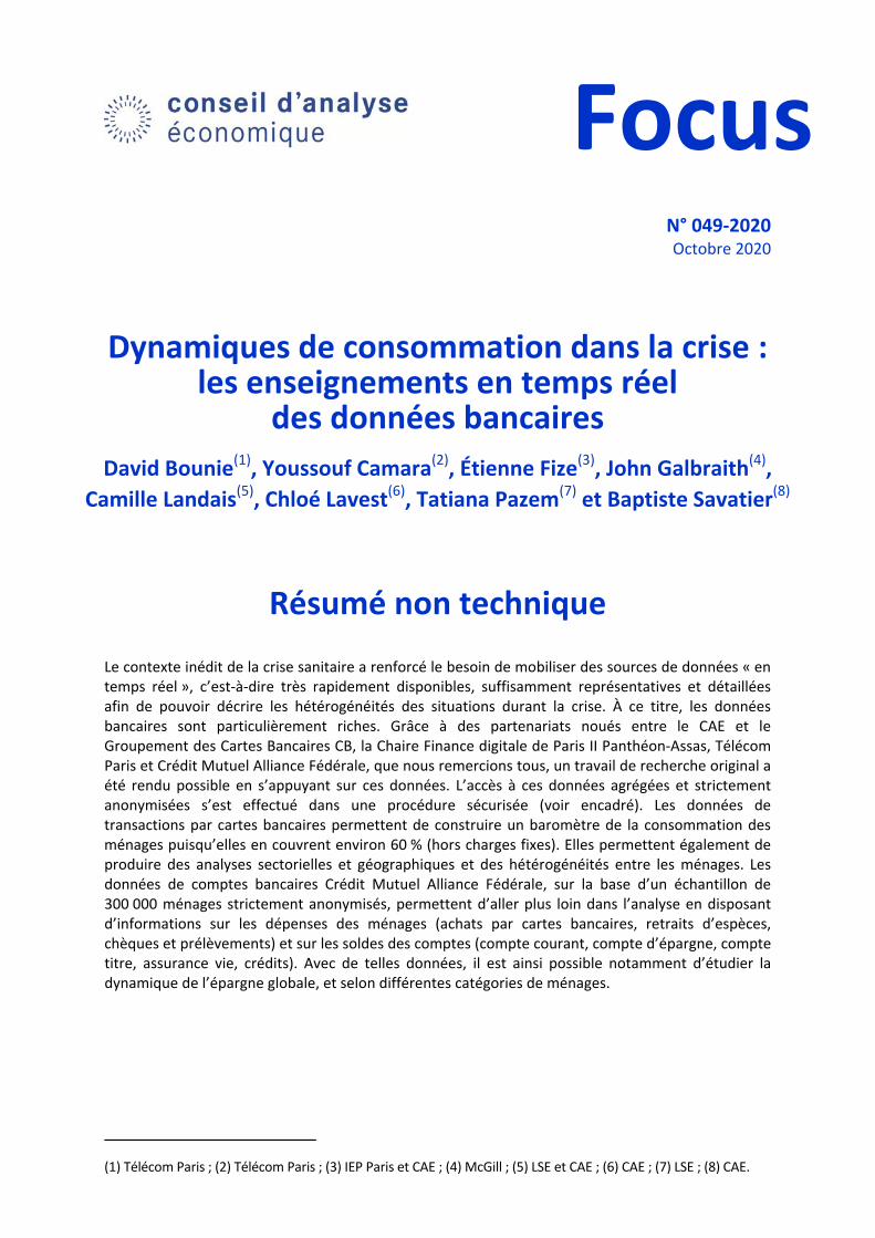
Les données de cartes bancaires permettent de suivre en temps réel l’évolution de la consommation en temps de crise Covid et de mieux comprendre ses déterminants. Après la chute de la consommation pendant le confinement qui a correspondu à une perte annualisée de 6,3 % par rapport à 2019, la consommation, telle que mesurée par les données de cartes bancaires, a rapidement rebondi avec depuis le déconfinement un retour à une consommation à un niveau normal avec même, en terme annualisé à nouveau, une augmentation de 0,7 %. Il n’y a pas eu pour autant de rattrapage de la consommation au niveau agrégé puisque le rebond ne compense pas du tout la perte pendant le confinement (voir graphique 1). C’est un point important qui est la source du risque accru de défaillance et qui suggère que nombre d’entreprises sont exposées à un risque de solvabilité et non pas seulement de liquidité.

Graphique 1. Dynamique globale des dépenses par carte

Source : Exploitation des données Groupement Cartes Bancaires CB.

Le rebond de la consommation a été particulièrement fort en juillet et août mais les données les plus récentes en particulier fin septembre montrent un léger essoufflement, en cohérence avec les récentes analyses de l’INSEE et de la Banque de France. Les mauvaises nouvelles sanitaires en sont peut‐être la cause même si elles n’ont pas, jusqu’ici, induit un comportement de retrait massif des consommateurs. De ce point de vue, ceux‐ci semblent donc s’adapter aux nouvelles conditions sanitaires. Un exemple de cette adaptation est la substitution des cartes bancaires au paiement en espèces.

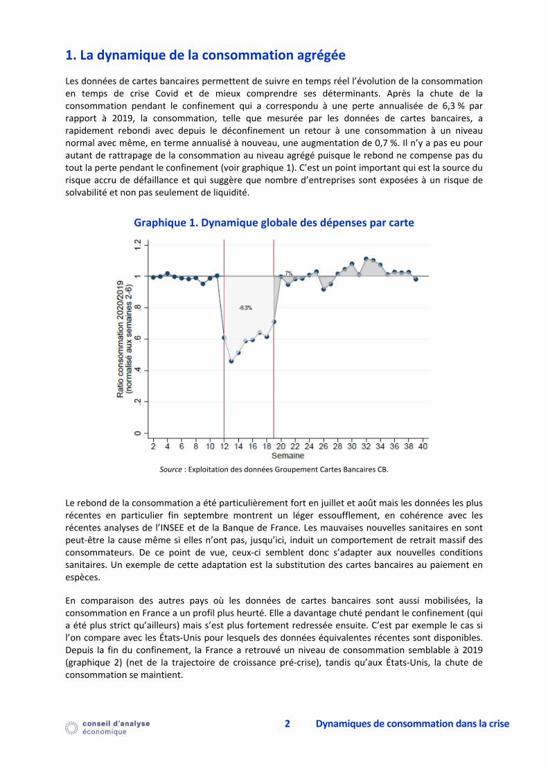
En comparaison des autres pays où les données de cartes bancaires sont aussi mobilisées, la consommation en France a un profil plus heurté. Elle a davantage chuté pendant le confinement (qui a été plus strict qu’ailleurs) mais s’est plus fortement redressée ensuite. C’est par exemple le cas si l’on compare avec les États‐Unis pour lesquels des données équivalentes récentes sont disponibles. Depuis la fin du confinement, la France a retrouvé un niveau de consommation semblable à 2019 (graphique 2) (net de la trajectoire de croissance pré‐crise), tandis qu’aux États‐Unis, la chute de consommation se maintient.


Graphique 2. Comparaisons internationales : États‐Unis vs France


2. La dynamique globale de l’épargne des ménages

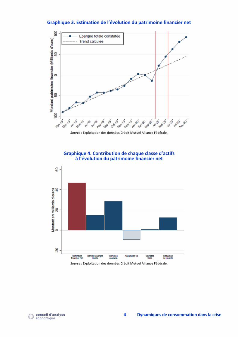
Grâce aux données de comptes bancaires, nous pouvons aussi analyser la dynamique de l’épargne. Nous estimons l’accumulation faite par les ménages depuis le confinement sur leurs comptes courants, comptes d’épargne, comptes d’assurance vie et comptes titres, nette des variations de leur dette. En déviation par rapport à la croissance de la période pré‐Covid (soit de fin février 2019 à fin février 2020), le surcroît d’épargne depuis le confinement est très important. Sur la base des données bancaires utilisées, qui ne peuvent qu’être partielles puisque les clients d’une banque peuvent placer une partie leur épargne au sein d’autres établissements bancaires, nous l’évaluons à un peu moins de 50 milliards d’euros fin août 2020 (voir graphique 3). Ce surcroît d’épargne s’est matérialisé surtout par une augmentation des soldes des comptes courants et des comptes d’épargne et par une diminution de la dette, très peu par une augmentation des comptes titres, tandis que l’assurance‐vie est en net recul (voir graphique 4).


Graphique 3. Estimation de l’évolution du patrimoine financier net

Source : Exploitation des données Crédit Mutuel Alliance Fédérale.

Graphique 4. Contribution de chaque classe d’actifs à l’évolution du patrimoine financier net



3. L’hétérogénéité sectorielle

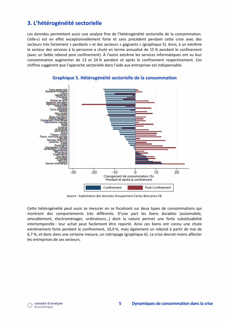
Les données permettent aussi une analyse fine de l’hétérogénéité sectorielle de la consommation. Celle‐ci est en effet exceptionnellement forte et sans précédent pendant cette crise avec des secteurs très fortement « perdants » et des secteurs « gagnants » (graphique 5). Ainsi, à un extrême le secteur des services à la personne a chuté en terme annualisé de 15 % pendant le confinement (avec un faible rebond post confinement). À l’autre extrême les services informatiques ont vu leur consommation augmenter de 13 et 24 % pendant et après le confinement respectivement. Ces chiffres suggèrent que l’approche sectorielle dans l’aide aux entreprises est indispensable.

Graphique 5. Hétérogénéité sectorielle de la consommation


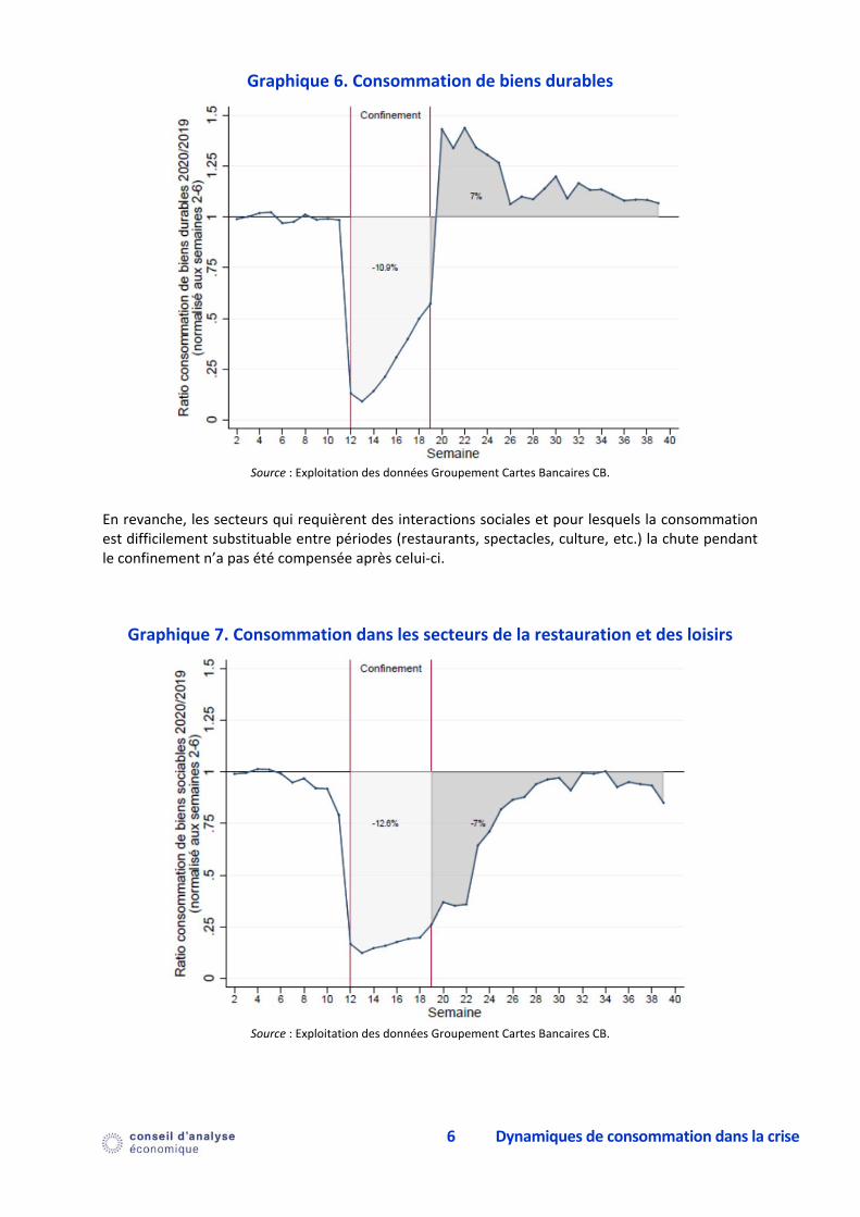
Cette hétérogénéité peut aussi se mesurer en se focalisant sur deux types de consommations qui montrent des comportements très différents. D’une part les biens durables (automobile, ameublement, électroménager, ordinateurs…) dont la nature permet une forte substituabilité intertemporelle : leur achat peut facilement être reporté. Ainsi ces biens ont connu une chute extrêmement forte pendant le confinement, 10,9 %, mais également un rebond à partir de mai de 6,7 %, et donc dans une certaine mesure, un rattrapage (graphique 6). La crise devrait moins affecter les entreprises de ces secteurs.


Graphique 6. Consommation de biens durables


En revanche, les secteurs qui requièrent des interactions sociales et pour lesquels la consommation est difficilement substituable entre périodes (restaurants, spectacles, culture, etc.) la chute pendant le confinement n’a pas été compensée après celui‐ci.

Graphique 7. Consommation dans les secteurs de la restauration et des loisirs



4. L’hétérogénéité entre les ménages

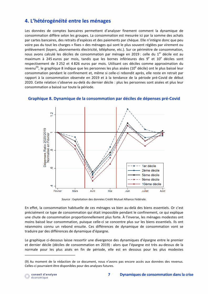
Les données de comptes bancaires permettent d’analyser finement comment la dynamique de consommation diffère selon les groupes. La consommation est mesurée ici par la somme des achats par cartes bancaires, des retraits d’espèces et des paiements par chèque. Elle n’intègre donc que peu voire pas du tout les charges « fixes » des ménages qui sont le plus souvent réglées par virement ou prélèvement (loyers, abonnements électricité, téléphone, etc.). Sur ce périmètre de consommation, nous avons calculé les déciles de consommation par ménage en 2019 : celle du 1er décile est au maximum à 245 euros par mois, tandis que les bornes inférieures des 9e et 10e déciles sont respectivement de 3 252 et 4 826 euros par mois. Utilisant ces déciles comme approximation du revenu(9),2le graphique 8 indique que les personnes les plus aisées (10e décile) ont le plus baissé leur consommation pendant le confinement et, même si celle‐ci rebondit après, elle reste en retrait par rapport à la consommation observée en 2019 et à la tendance de la période pré‐Covid de début 2020. Cette relation s’observe au‐delà du dernier décile : plus les personnes sont aisées et plus leur consommation a baissé sur toute la période.

Graphique 8. Dynamique de la consommation par déciles de dépenses pré‐Covid


En effet, la consommation habituelle de ces ménages va bien au‐delà des biens essentiels. Or c’est précisément ce type de consommation qui était impossible pendant le confinement, ce qui explique une chute de consommation proportionnellement plus forte. À l’inverse, les ménages modestes ont moins baissé leur consommation, puisque celle‐ci se concentre plus sur les biens essentiels. Ils ont néanmoins connu un rebond ensuite. Ces différences de dynamique de consommation vont se traduire par des différences de dynamique d’épargne.

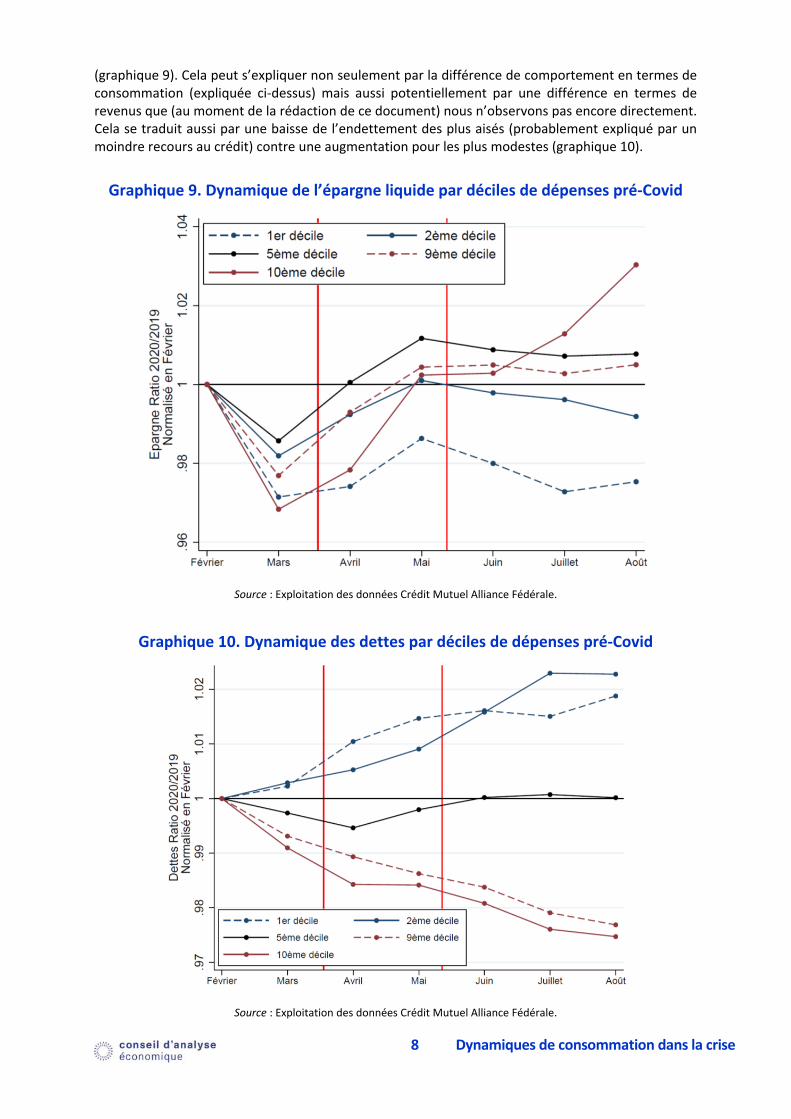
Le graphique ci‐dessous laisse ressortir une divergence des dynamiques d’épargne entre le premier et dernier décile (déciles de consommation en 2019) : alors que l’épargne est très au‐dessus de la normale pour les plus aisés en fin de période, elle est en dessous pour les plus modestes

(9)2Au moment de la rédaction de ce document, nous n’avons pas encore accès aux données des revenus. Celles‐ci pourraient être disponibles pour des analyses futures.


(graphique 9). Cela peut s’expliquer non seulement par la différence de comportement en termes de consommation (expliquée ci‐dessus) mais aussi potentiellement par une différence en termes de revenus que (au moment de la rédaction de ce document) nous n’observons pas encore directement. Cela se traduit aussi par une baisse de l’endettement des plus aisés (probablement expliqué par un moindre recours au crédit) contre une augmentation pour les plus modestes (graphique 10).

Graphique 9. Dynamique de l’épargne liquide par déciles de dépenses pré‐Covid


Graphique 10. Dynamique des dettes par déciles de dépenses pré‐Covid



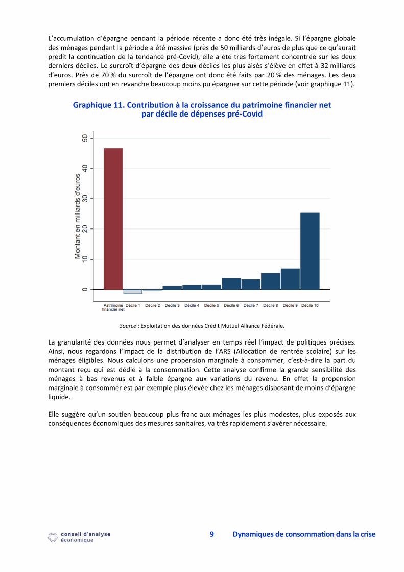
L’accumulation d’épargne pendant la période récente a donc été très inégale. Si l’épargne globale des ménages pendant la période a été massive (près de 50 milliards d’euros de plus que ce qu’aurait prédit la continuation de la tendance pré‐Covid), elle a été très fortement concentrée sur les deux derniers déciles. Le surcroît d’épargne des deux déciles les plus aisés s’élève en effet à 32 milliards d’euros. Près de 70 % du surcroît de l’épargne ont donc été faits par 20 % des ménages. Les deux premiers déciles ont en revanche beaucoup moins pu épargner sur cette période (voir graphique 11).

Graphique 11. Contribution à la croissance du patrimoine financier net par décile de dépenses pré‐Covid


La granularité des données nous permet d’analyser en temps réel l’impact de politiques précises. Ainsi, nous regardons l’impact de la distribution de l’ARS (Allocation de rentrée scolaire) sur les ménages éligibles. Nous calculons une propension marginale à consommer, c’est‐à‐dire la part du montant reçu qui est dédié à la consommation. Cette analyse confirme la grande sensibilité des ménages à bas revenus et à faible épargne aux variations du revenu. En effet la propension marginale à consommer est par exemple plus élevée chez les ménages disposant de moins d’épargne liquide.

Elle suggère qu’un soutien beaucoup plus franc aux ménages les plus modestes, plus exposés aux conséquences économiques des mesures sanitaires, va très rapidement s’avérer nécessaire.


5. Conclusion

L’utilisation et l’analyse de données bancaires microéconomiques en temps réel, inédit en France, permet un suivi précieux pour la compréhension des effets de la crise sur les ménages français. Cette analyse mérite d’être continuée. Ces données, mises à disposition récemment, recèlent encore un fort potentiel inexploité. Les auteurs souhaitent approfondir les analyses décrites ci‐dessus, notamment en termes d’hétérogénéité des réponses face à la crise, encore mal captée par les classifications économiques usuelles (âge, profession et catégories socioprofessionnelles). L’exploitation plus fine des données pourrait également conduire à un calibrage précis des politiques publiques en identifiant les publics prioritaires de populations particulièrement soumises à la crise, notamment en termes de chute du revenu.

Encadré. Crédit Mutuel Alliance Fédérale et Groupement Cartes Bancaires CB

Première banque à adopter le statut d’entreprise à mission, Crédit Mutuel Alliance Fédérale a contribué à cette étude par la fourniture de données de comptes bancaires sur la base d’un échantillon de ménages par tirage aléatoire. Toutes les analyses réalisées dans le cadre de cette étude ont été effectuées sur des données strictement anonymisées sur les seuls systèmes d’information sécurisés du Crédit Mutuel en France. Pour Crédit Mutuel Alliance Fédérale, cette démarche « s’inscrit dans le cadre des missions qu’il s’est fixé :

contribuer au bien commun en œuvrant pour une société plus juste et plus durable : en participant à l’information économique, Crédit Mutuel Alliance Fédérale réaffirme sa volonté de contribuer au débat démocratique ;

protéger l’intimité numérique et la vie privée de chacun : Crédit Mutuel Alliance Fédérale veille à la protection absolue des données de ses clients ».

Le Groupement des Cartes Bancaires CB, Groupement d’Intérêt Économique qui définit les modalités de fonctionnement du schéma de paiement par carte CB (physique ou dématérialisée dans le mobile) a également contribué à cette étude par la fourniture de ses données (agrégées) et par la possibilité de solliciter des traitements sur des données individuelles anonymisées dans un espace strictement sécurisé et dans le cadre de son partenariat avec la Chaire Finance Digitale. « Ce partenariat entre CB et le monde académique va permettre de développer de nouvelles filières de compétence. Il reflète aussi la démarche citoyenne et responsable de CB, qui a pour volonté de servir l’intérêt général et favoriser l’inclusion sociale et sociétale », déclare Philippe Laulanie, Directeur général de CB.

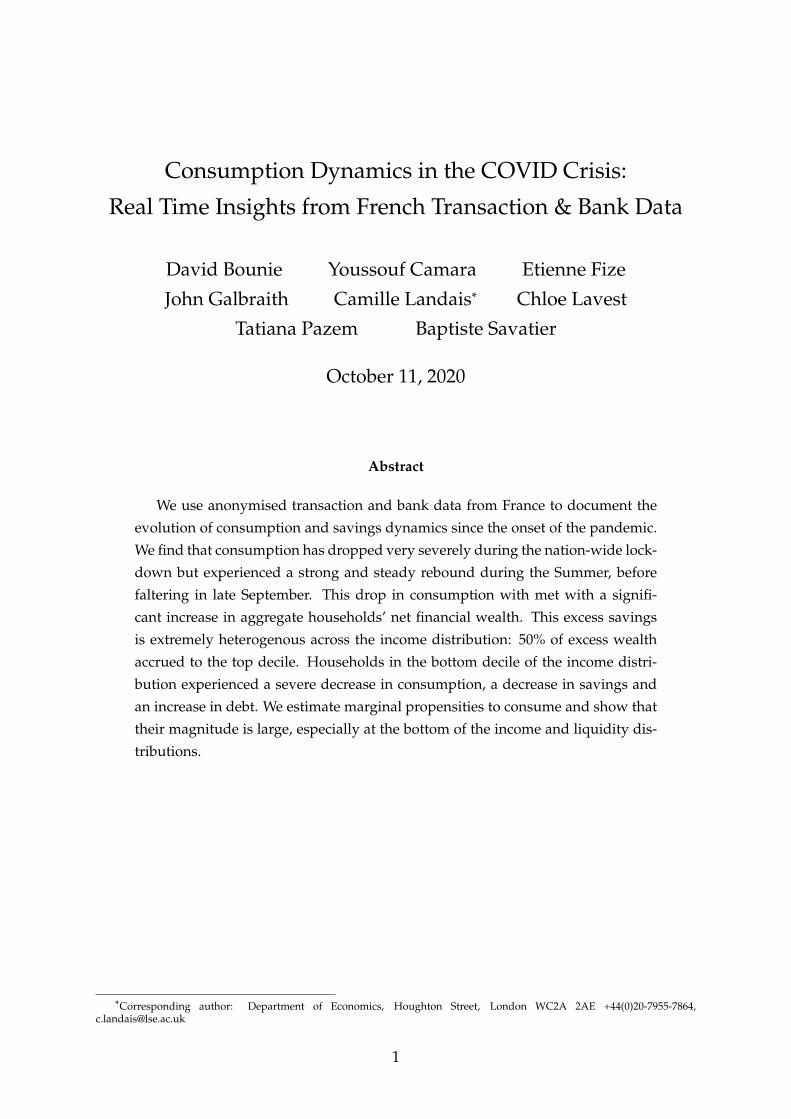
Consumption Dynamics in the COVID Crisis:

Real Time Insights from French Transaction & Bank Data

David Bounie Youssouf Camara Etienne Fize

John Galbraith Camille Landais* Chloe Lavest

Tatiana Pazem Baptiste Savatier

October 11, 2020

Abstract

We use anonymised transaction and bank data from France to document the

evolution of consumption and savings dynamics since the onset of the pandemic.

We find that consumption has dropped very severely during the nation-wide lock-

down but experienced a strong and steady rebound during the Summer, before

faltering in late September. This drop in consumption with met with a signifi-

cant increase in aggregate households’ net financial wealth. This excess savings

is extremely heterogenous across the income distribution: 50% of excess wealth

accrued to the top decile. Households in the bottom decile of the income distri-

bution experienced a severe decrease in consumption, a decrease in savings and

an increase in debt. We estimate marginal propensities to consume and show that

their magnitude is large, especially at the bottom of the income and liquidity dis-

tributions.

*Corresponding author: Department of Economics, Houghton Street, London WC2A 2AE +44(0)20-7955-7864,[email protected]

1

1 Introduction

The explosive dynamics of the coronavirus shock has created a new historic need for“extreme nowcasting” to monitor the impact of the shock on the economy. This in turnrequires access to new data that are quickly available (for reactivity), representative(for robustness) and granular (to allow for rich distributional analysis, as well as quasi-experimental analysis to learn about mechanisms).

Furthermore, the covid shock is unprecedented in both its magnitude and its nature.This poses a series of original issues to policy-makers in their response to the crisis.How is the economic shock distributed in the population? What is the causal role ofhealth risk in explaining behaviors? How much are consumption and savings behav-ior driven by precautionary savings in response to the significant rise in uncertaintyregarding future income and employment dynamics? Etc.

In this work, we offer insights coming from the use of original anonymous and de-identified transaction and bank data in the French context. The data comes from twounique sources. First, from the universe of card transactions from the French consor-tium of card providers “Groupement Cartes Bancaires CB” (CB thereafter). Second,from a large balanced panel of 300,000 households randomly sampled from the clientsof the French Bank Credit Mutuel Alliance Federale (CM thereafter).1

We first investigate the dynamics of aggregate transactions. We find that card transac-tion expenditures experienced a severe decline of about 50% during the nation-widelockdown period that started in mid-March in France, and lasted until mid-May. In-terestingly, we find that after that initial phase, expenditures bounced back almostimmediately to their 2019 levels, and remained steady throughout the summer. Inthat sense, the French recovery in terms of consumption has been much stronger thanin other countries such as the US or the UK. There is nevertheless an extreme amountof sectoral heterogeneity in the dynamics of expenditures, which is a unique featureof the covid-induced recession. Furthermore, there are clear signs that consumptionexpenditures have been faltering in the last weeks of September, as a second epidemicwave was gaining momentum in France.

Using the richness of the CM data, we also explore the dynamics of financial wealthand savings behavior during the crisis. We find that aggregate financial wealth hasincreased by about e50 billions since the onset of the crisis, compared to the counter-factual of a prolongation of the 2019 trend. Interestingly, most of this excess financialwealth is accounted for by an increase in liquid savings. Moving to distributional

1All data is de-identified, and accessed through secure internal IT servers. We provide all details onthe data, and on the procedures for data access and for preserving data privacy in the Data section ofthis paper, as well as in the Appendix.

2

analysis, we find that more than 50% of this excess “savings” accrued to householdsin the top decile of the income distribution. At the bottom of the distribution, con-sumption and savings have both decreased since the start of the pandemic, indicativeof severe income shocks experienced by these households, despite the social insuranceand welfare transfer policies put in place by the French government since the start ofthe crisis.

Finally, we also show how this unique source of data can be used to explore therespective role of three potential drivers of consumption dynamics. We investigatethe importance of income dynamics and income expectations by estimating marginalpropensities to consume, taking advantage of the granularity of the CM data, com-bined with quasi-experimental variation in welfare transfer payments. We find largebut heterogeneous MPCs, with households at the bottom of the liquid savings distri-bution being particularly sensitive to additional cash-on-hand. We then turn to explor-ing the role of health risk, vis-a-vis that of lockdown and restriction policies. We findrelatively little role of health risk perceptions on consumption dynamics on average,but a strong role for lockdown policies.

The remainder of the paper is organized as follows. Section 2 presents the data, Section3 analyzes the evolution of aggregate consumption and savings. Section 4 documentssectoral heterogeneity, while section 5 delves into the distributional impact of the cri-sis. Finally, section 6 explores the mechanisms driving consumption dynamics sincethe beginning of the covid crisis.

2 Data

2.1 Carte Bancaires

Cartes Bancaires CB is one of the leading consortium of payment service providers,banks and e-money institutions. It was created by the French banks in 1984, and by2019 had more than 100 members. As of 2019 there were more than 71.1 million CBcards in use in the CB system, and 1.8 million CB-affiliated merchants.

Thanks to a partnership with Cartes Bancaires CB, we are able to observe the universeof CB card transactions at a very granular level. A CB card transaction is characterizedby its amount, the precise time and date of the transaction, the geographical locationof the merchant, the statistical classification of the type of purchase, and the type ofpurchasing channel used during the transaction, i.e. off-line or online. By definition,all the other card transactions carried out with payment card schemes such as Visa or

3

MasterCard are not covered and part of the analysis, as they are not CB card transac-tion. Similarly, the payments made by checks, direct debits and credit transfers are nottransactions covered by the CB card network.

The data set of CB card transactions is exceptional in its coverage, allowing us to cap-ture a significant proportion of all consumer expenditure in France. To appreciate therichness of the Cartes Bancaires CB data, consider a few comparisons with nationalstatistics provided for the full year 2019 by the National Institute of Statistics and Eco-nomic Studies (INSEE). GDP in France in 2019 was estimated as e 2,427 billion, withe 1,254 billion (52 percent of GDP) representing household consumption expenditure.Excluding fixed charges (rents, financial services, insurances) from household con-sumption expenditure, as these are typically paid by checks, direct debits and credittransfers, the remaining part of consumer expenditure amounts to e 828 billion (34percent of GDP). Comparing these figures with total CB card payments (e 494 billion),the value of CB card payments represents 20 percent of French GDP, 39 percent oftotal household consumption expenditure, and finally 60 percent of total householdconsumption expenditure excluding fixed charges. CB card transactions thus capturesthe most cyclical part of household consumption expenditure, which is very useful foreconomic nowcasting.

The real-time and detailed information on timing and location of the transaction, thenature of the merchant, allows us to provide fine-grained descriptions of consumptionfluctuations, and to contrast consumption patterns along the geographical and sectoraldimensions.2 For more details on the CB data, see Bounie, Camara and Galbraith[2020], who provide a detailed analysis of consumption dynamics in the early monthsof the crisis.

2.2 Credit Mutuel Alliance Fédérale

Sampling

The data used in this paper comes from a balanced panel of 300,000 randomly se-lected clients of the French National retail bank CIC, a subsidiary of Crédit MutuelAlliance Fédérale. As opposed to the Crédit Mutuel which is deeply rooted in the Eastof France, the CIC is less regionally concentrated and has more than 2,000 agenciesspread across the country.

The sampling procedure was the following. We selected customers according to theirage and department (French administrative geographical area called “département”)

2We limit the sample to Metropolitan France, which excludes the overseas territories.

4

of residency. We defined 6 age groups (18-25, 26-35, 36-45, 46-55, 56-65 and 66+). Fromeach of the 94 departments and age groups we randomly selected a certain number ofcustomers. For the 31 most populated departments in France we selected 1,000 cus-tomers per cell (age-groupe - department). For the next 26, we selected 500, for the next13 300 and finally 100 for the last 24 departments. This sampling procedure ensured abetter representativity of the sample but also guaranteed anonymity, by making surethat the fraction of sampled customers in each cell did not exceed a specific threshold.

Furthermore, the customers were chosen out of a sub-sample of all CIC clients. Thecustomers had to be “principal customers”, meaning that the CIC is their main bankwhere they domiciliate their income and main assets and credits. They had to be aphysical entity and alive. We do have self-employed individuals in our sample but nofirms. All customers in our sample had to be customers at least before January 2019.We excluded residents of Corsica, French overseas territories and customers outsideof France. Finally we also excluded employees of Crédit Mutuel Alliance Fédérale andindividuals banned from holding a bank account.

The sampling resulted in a little over 300,000 customers defined at the group level (i.ehousehold level) which amounts to approximately 550,000 individuals. In cases wherethe household composition changed (marriage, divorce ...), we kept in the sample allof the initial members of the groups. The sampling was performed in June 2020.

Reweighting

In order for our sample to better match national data, we reweight each age-groupdepartment cell to match French census data from INSEE. Note that for now, we onlyuse age and geography as observables characteristics in our reweighting approach, butmore sophisticated approaches can be used, to match other aggregate or distributionalstatistics in the French population.

Data structure

We use pseudo-anonymized data located on a secure distant server.3

We were granted access of three tables containing information on card expenditures,cash withdrawals, check payments, bank balances, savings accounts, equities, life in-surances and household debts. Moreover we have some information on wire transfersand for the year 2020 we have information on direct debits and daily information on

3See appendix for more detail information on data access and the partnership with Crédit MutuelAlliance Fédérale.

5

card expenditures that allows us to know in which sector (MCC classification) thespending was made.

We also have access to some information regarding the account owner and householdmembers : department, age, socio-professional category (PCS)4, marital status andwhether or not the individual is self-employed. Note that the definition of householdsin the CM data is different from the standard INSEE definition usually retained inFrench survey data.5.

Descriptive statistics

Our sampling strategy led to an overrepresentation of young people and an underrep-resentation of older people. Appendix Table 1 provides descriptive statistics for ouroriginal sample, as well as our reweighted sample, and then compares these statisticsto external INSEE data on the universe of the French population. The reweighting pro-cedure allows us to get a more representative sample of the French population. Butwe still slightly underrepresent retirees.6

4“Nomenclature des Professions et catégories socio-professionnelles” which can translate to“Nomenclature of Professions and Socioprofessional Categories”

5Indeed, whereas INSEE considers that a household is defined by a shared home, and not by kin-ship, allowing roomates, for example, to form a unique household, this is not the case in the CréditMutuel Alliance Fédérale databases. Their definition of a household is much more restricted: onlyblood or marriage related people are considered to be a unit. Moreover, children turning 18 are bydefault transferred to a new household unit even though they may still be living with their parents.

6Our interpretation of this deviation is that even though the sample has been reweighted and doesbetter at comparing with the actual percentage of older people in the French population (66+ peopleattainted 21.13% after the weighting procedure against 16.70% before it for a total of 24.61% as reportedby the INSEE census in 2018), because the Crédit Mutuel Alliance Fédérale data must be updated bythe account owners themselves, few of them actually declare their retirement right away, hence PCSvariables are often updated with significant delay at retirement.

6

3 Aggregate Consumption & Savings Dynamics

3.1 Consumption

We start by documenting the evolution of aggregate consumption dynamics in Francesince the beginning of the pandemic. We focus on aggregate credit card expendituresmeasured in the CB data. We aggregate transactions at the weekly level. To deal withseasonality, we divide aggregate transactions in week t of 2020 by aggregate transac-tions in the exact same week t in 2019: C2020

t /C2019t . We further take away the general

trend in aggregate consumption between 2019 and 2020. To this effect, we normal-ize these expenditure ratios by the average ratio between week 2 and week 6 in 2020:C̄2020

t∈[2;6]/C̄2019t∈[2;6]. In other words, we assume that the overall trend observed in expen-

ditures between the first weeks of 2020 and the first weeks 2019 would have contin-ued absent the COVID crisis. We then report ct =

C2020t /C2019

tC̄2020

t∈[2;6]/C̄2019t∈[2;6]

, which measures how

consumption deviates from its 2019 level, once accounting for the general trend thatwould have occured between 2019 and 2020 absent the pandemic.

Sharp Decline & Steep Recovery Figure 1 shows the evolution of credit card trans-actions from the CB data since the start of 2020. The first red line corresponds to thestart of the nation-wide lockdown in France (week 12) and the second red line cor-responds to the end of the lockdown in week 19. The figure shows that aggregatetransactions did not experience much of a decline before the start of the lockdown.But the lockdown was associated with a brutal and severe decline in transactions, ofabout 50%. Transactions remained extremely depressed throughout the seven weeksof lockdown despite a small improvement after the initial sharp contraction of week13. Interestingly, aggregate consumption bounced back immediately to pre-crisis lev-els as soon as the lockdown ended, and has been stable at this level ever since. Theredoes not seem to be signs of a decrease in expenditures since late August, as a secondwave of covid infections has been quickly spreading across the country.

A few important lessons emerge from these patterns of aggregate consumption dy-namics. First, the overall contraction in spending during the lockdown has been mas-sive in France. If we cumulate the aggregate amount of spending “lost” from week 12to week 19 (the light grey area in Figure 1), this corresponds to a 6.3% loss in annualspending. Second, although the recovery in credit card transactions has been quickand steady since the end of the lockdown, transactions have reached their pre-crisislevel, but did not overshoot: there is no sign of intertemporal substitution at the ag-gregate level. In other words, the 6.3% loss in annual spending during the lockdownis a permanent loss. Third, there does not seem to be strong signs of correlation in the

7

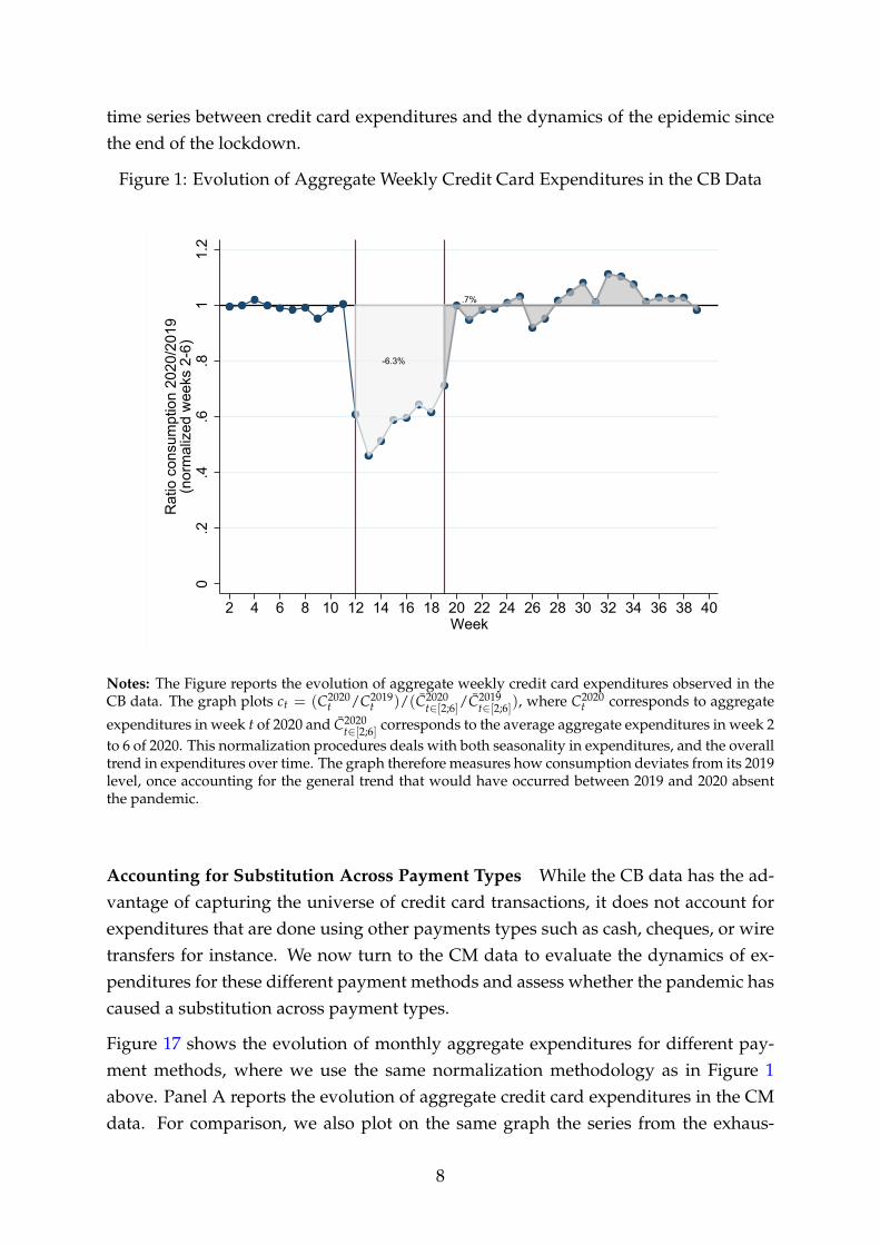
time series between credit card expenditures and the dynamics of the epidemic sincethe end of the lockdown.

Figure 1: Evolution of Aggregate Weekly Credit Card Expenditures in the CB Data

-6.3%

.7%

0.2

.4.6

.81

1.2

Rat

io c

onsu

mpt

ion

2020

/201

9(n

orm

aliz

ed w

eeks

2-6

)

2 4 6 8 10 12 14 16 18 20 22 24 26 28 30 32 34 36 38 40Week

Notes: The Figure reports the evolution of aggregate weekly credit card expenditures observed in theCB data. The graph plots ct = (C2020

t /C2019t )/(C̄2020

t∈[2;6]/C̄2019t∈[2;6]), where C2020

t corresponds to aggregate

expenditures in week t of 2020 and C̄2020t∈[2;6] corresponds to the average aggregate expenditures in week 2

to 6 of 2020. This normalization procedures deals with both seasonality in expenditures, and the overalltrend in expenditures over time. The graph therefore measures how consumption deviates from its 2019level, once accounting for the general trend that would have occurred between 2019 and 2020 absentthe pandemic.

Accounting for Substitution Across Payment Types While the CB data has the ad-vantage of capturing the universe of credit card transactions, it does not account forexpenditures that are done using other payments types such as cash, cheques, or wiretransfers for instance. We now turn to the CM data to evaluate the dynamics of ex-penditures for these different payment methods and assess whether the pandemic hascaused a substitution across payment types.

Figure 17 shows the evolution of monthly aggregate expenditures for different pay-ment methods, where we use the same normalization methodology as in Figure 1above. Panel A reports the evolution of aggregate credit card expenditures in the CMdata. For comparison, we also plot on the same graph the series from the exhaus-

8

tive CB data. The two series display similar dynamics, although the CM series isa little more volatile. Panel B focuses on payments by cheque and shows that suchpayments have decreased more than credit card payments during the lockdown. Fur-thermore, they are still at a level that is 5 to 10% lower than pre-crisis level. PanelC shows similar patterns for cash withdrawals, which are currently 15% below theirpre-crisis levels. This suggests that consumers have significantly moved away fromcash payments in response to the pandemic. In panel D, we show the dynamics of to-tal expenditures, that is credit card transactions, cash withdrawals, cheques (XX whatabout prelevements automatiques etc??). The graph confirms that accounting for allpayment methods, the level of consumer expenditures has bounced back vigorouslyafter the sharp contraction of the lockdown. However, the level of total expendituresis, after the lockdown, about 2 to 3% lower than what it would have been absent thepandemic.

International Comparisons We now compare the evolution of consumption dynam-ics in France and in a series of countries for which similar data is available. The datafor Denmark and Sweden comes from Andersen et al. [2020], the data for the US comesfrom Chetty et al. [2020] and the data from the UK is from Hacioglu, Känzig and Surico[2020]. For all countries, we use the same normalization as in Figure 1. Note that allfive countries experienced a roughly similar timing for their first wave of the covidepidemic.

Several important insights transpire from this comparison. First, in the second halfof March 2020, all five countries witnessed a sudden drop in spending, and this dropwas of roughly similar magnitude. This happened despite the drastically different lev-els of severity of the restrictions put in place at that time across these five countries.This evidence prompted the interpretation that this is the epidemic, and not policies,that caused the severe contraction in spending (e.g. XX johanesen paper). Inter-estingly though, after this initial phase that saw remarkably similar dynamics acrosscountries, consumer transactions have been experiencing drastically different patternsacross countries. These differences suggest that the policy paths chosen by the differ-ent countries have had a significant impact on the dynamics of aggregate consump-tion. We see for instance that, countries like France, which entered a strict nation-widelockdown, had a much more severe decrease in aggregate transactions, than countriesthat did not mandate nation-wide lockdowns like Sweden or the US. But we also seethat after this initial phase of severe decline in consumption, the recovery in creditcard transactions has been much more rapid in France than anywhere else. In the UKfor instance, overall consumption remained heavily depressed throughout May andJune. In panel B, we focus on the comparison between France and the US. Due to its

9

severe lockdown, France experienced until May a decline in expenditures relative tothe US equivalent to 2.6% in annual term (i.e. light grey area in panel B). But sincethe end of the lockdown, the quick recovery has made up for all this loss: French ex-penditures have recovered 2.6% in annual term relative to the US. As a consequence,so far, the cumulated decline in consumption expenditures over the year 2020 appearsequivalent in both countries despite drastically different trajectories.

Overall, evidence from Figure 2 confirms that policies do actually matter, and that theirimpact must be measured by taking into account their full long run dynamic effects.

10

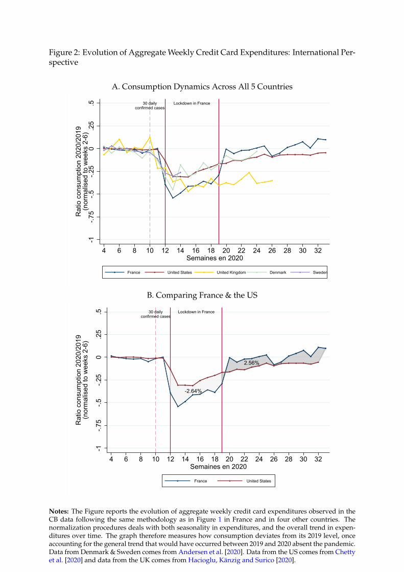
Figure 2: Evolution of Aggregate Weekly Credit Card Expenditures: International Per-spective

A. Consumption Dynamics Across All 5 Countries

30 dailyconfirmed cases

Lockdown in France

-1-.7

5-.5

-.25

0.2

5.5

Rat

io c

onsu

mpt

ion

2020

/201

9(n

orm

alis

ed to

wee

ks 2

-6)

4 6 8 10 12 14 16 18 20 22 24 26 28 30 32Semaines en 2020

France United States United Kingdom Denmark Sweden

B. Comparing France & the US

-2.64%

2.56%

30 dailyconfirmed cases

Lockdown in France

-1-.7

5-.5

-.25

0.2

5.5

Rat

io c

onsu

mpt

ion

2020

/201

9(n

orm

alis

ed to

wee

ks 2

-6)

4 6 8 10 12 14 16 18 20 22 24 26 28 30 32Semaines en 2020

France United States

Notes: The Figure reports the evolution of aggregate weekly credit card expenditures observed in theCB data following the same methodology as in Figure 1 in France and in four other countries. Thenormalization procedures deals with both seasonality in expenditures, and the overall trend in expen-ditures over time. The graph therefore measures how consumption deviates from its 2019 level, onceaccounting for the general trend that would have occurred between 2019 and 2020 absent the pandemic.Data from Denmark & Sweden comes from Andersen et al. [2020]. Data from the US comes from Chettyet al. [2020] and data from the UK comes from Hacioglu, Känzig and Surico [2020].

3.2 Household Balance Sheet & Savings Dynamics

The household balance-sheet data from CM allows us to also investigate the dynamicsof household savings during the pandemic. We start by explaining the content of thehousehold balance-sheet data currently available. What we observe in the data are:

• WBit : balances of all bank accounts held with CM in month t

• WSit : balances on all liquid savings accounts held with CM in month t (e.g. “comptes

sur livret”, PEL, etc)

• WMit : balances of all mutual funds held with CM in month t (e.g. “comptes

titres”)

• Dit: balance of all household debt held with CM in month t (e.g. consumer loans,credit card debt, etc.) also including mortgage

From this information, we create a measure of household financial wealth net of debt

Wit = WBit + WS

it + WMit − Dit (1)

It is important to acknowledge a couple of important limitations of this measure. First,we do not observe the balance of accounts or assets held outside the bank. Second,there are important components of the household balance sheet that we do not ob-serve. In particular, at this point, we do not observe the value of real estate wealth WR

itowned by households.In that sense, our measure is not a comprehensive measure ofhousehold wealth, but a measure of net financial wealth.

We start by documenting the evolution of our measure of household financial wealth.But we are also interested in measuring savings, that is, in separating what, in thedynamics of household wealth, is driven by the dynamics of asset prices, and what isdue to active savings behaviors of household.

To define households’ active savings, it is useful to start from the definition of thehousehold budget constraint:

Cit = Zit −∑k

pkt [Aikt − Aikt−1]︸︷︷︸Savings

, (2)

where Zit captures all sources of income net of taxes and transfers, Ait = Ai1t, .., AiKt

denotes the portfolio of assets and pt = pi1t, .., piKt the corresponding vector of pricesat which they are traded. We can re-write the asset component of the identity in (2) as

pkt∆Aikt = ∆Wikt − ∆pkt Aikt−1,

12

where we use the difference notation ∆Xt = Xt − Xt−1. The above expression high-lights that only the active rebalancing of assets participates in the flow of active sav-ings. To measure active savings, we therefore need to substract from the change inthe value of the portfolio (∆Wit) the passive gains on assets induced by changes in theprice of these assets.

In practice, we do not observe the prices for each individual asset held by each house-hold to offer a household-specific measure of passive capital gains on each asset class.We therefore operationalize our measure of savings in the following way:

St = ∆Wit −

Passive K gains︷︸︸︷∆pt

pt−1·WM

it−1 − YSit + rt · Dit︸︷︷︸

Interests on debt

That is, we use the evolution of average prices of stocks to measure passive capitalgains on wealth held in mutual funds (WM

it ), and the average interest rate on debtto measure the contribution of the change in the price of household debt. YS

it is theobserved interest income on liquid savings accounts.

Kolsrud, Landais and Spinnewijn [2020] and Eika, Mogstad and Vestad [2020] pro-vide a detailed discussion of the measurement error created by using average (ratherthan individual-specific) price indices to retrieve savings and consumption flows fromhousehold balance-sheet data.

Dynamics of Net Financial Wealth Wt. In Figure 3, we present the evolution of totalnet financial wealth, normalized to zero at the end of January 2020. Note that aggre-gate wealth is computed using our designed sample weights, so that we interpret thistotal as representative of total net financial wealth (as defined in (1)) in the populationliving in the French Metropolitan area. The Figure shows that, after a sharp initial dipin March 2020, Wt rebounded strongly. Overall, Wt has grown by about e90 billionsbetween January 2020 and beginning of September 2020. The Figure also highlightsthat Wt was already trending strongly upwards in 2019. We report in red on the graphthe linear trend in Wt computed over the period January 2019 to January 2020. Wemeasure the effect of the pandemic shock on wealth Wt as the deviation from thistrend. We find that total net financial household wealth has increased by e5X billionsin the aftermath of the covid crisis, relative to the counterfactual of what would havehappened if it had continue to grow according to its 2019 trend.

In Figure 4, we decompose the evolution of net financial wealth Wt into its differentcomponents. For each component Wk

t observed in month t, we deal with both season-ality and trend using the same methodology as in Figure 1. That is, we report the ratio

13

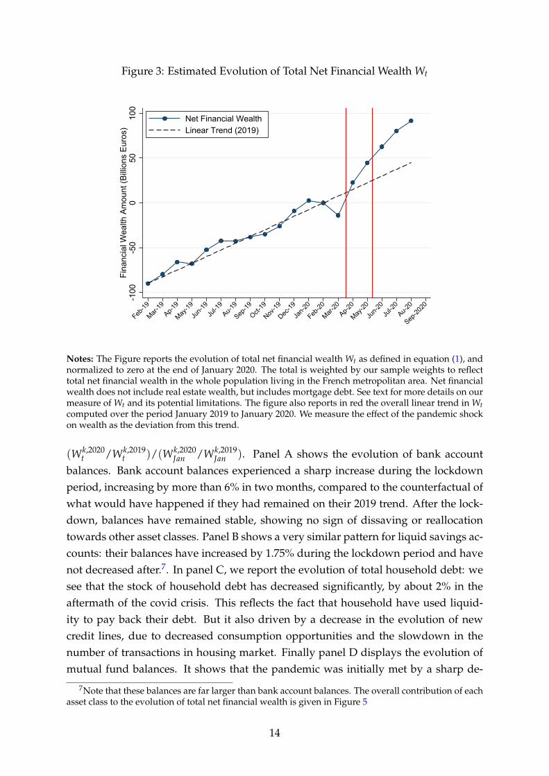
Figure 3: Estimated Evolution of Total Net Financial Wealth Wt

-100

-50

050

100

Fina

ncia

l Wea

lth A

mou

nt (B

illion

s Eu

ros)

Feb-19

Mar-19

Ap-19

May-19

Jun-1

9Ju

l-19

Au-19

Sep-19

Oct-19

Nov-19

Dec-19

Jan-2

0

Feb-20

Mar-20

Ap-20

May-20

Jun-2

0Ju

l-20

Au-20

Sep-20

20

Net Financial WealthLinear Trend (2019)

Notes: The Figure reports the evolution of total net financial wealth Wt as defined in equation (1), andnormalized to zero at the end of January 2020. The total is weighted by our sample weights to reflecttotal net financial wealth in the whole population living in the French metropolitan area. Net financialwealth does not include real estate wealth, but includes mortgage debt. See text for more details on ourmeasure of Wt and its potential limitations. The figure also reports in red the overall linear trend in Wtcomputed over the period January 2019 to January 2020. We measure the effect of the pandemic shockon wealth as the deviation from this trend.

(Wk,2020t /Wk,2019

t )/(Wk,2020Jan /Wk,2019

Jan ). Panel A shows the evolution of bank accountbalances. Bank account balances experienced a sharp increase during the lockdownperiod, increasing by more than 6% in two months, compared to the counterfactual ofwhat would have happened if they had remained on their 2019 trend. After the lock-down, balances have remained stable, showing no sign of dissaving or reallocationtowards other asset classes. Panel B shows a very similar pattern for liquid savings ac-counts: their balances have increased by 1.75% during the lockdown period and havenot decreased after.7. In panel C, we report the evolution of total household debt: wesee that the stock of household debt has decreased significantly, by about 2% in theaftermath of the covid crisis. This reflects the fact that household have used liquid-ity to pay back their debt. But it also driven by a decrease in the evolution of newcredit lines, due to decreased consumption opportunities and the slowdown in thenumber of transactions in housing market. Finally panel D displays the evolution ofmutual fund balances. It shows that the pandemic was initially met by a sharp de-

7Note that these balances are far larger than bank account balances. The overall contribution of eachasset class to the evolution of total net financial wealth is given in Figure 5

14

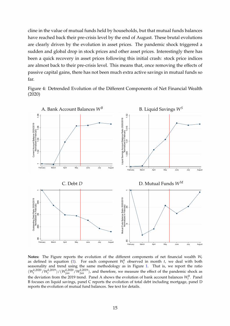
cline in the value of mutual funds held by households, but that mutual funds balanceshave reached back their pre-crisis level by the end of August. These brutal evolutionsare clearly driven by the evolution in asset prices. The pandemic shock triggered asudden and global drop in stock prices and other asset prices. Interestingly there hasbeen a quick recovery in asset prices following this initial crash: stock price indicesare almost back to their pre-crisis level. This means that, once removing the effects ofpassive capital gains, there has not been much extra active savings in mutual funds sofar.

Figure 4: Detrended Evolution of the Different Components of Net Financial Wealth(2020)

A. Bank Account Balances WB B. Liquid Savings WS

11.

021.

041.

061.

08

Cur

rent

Acc

ount

Bal

ance

202

0/20

19N

orm

aliz

ed in

Feb

ruar

y

February March April May June July August

11.

005

1.01

1.01

51.

02

Liqu

id S

avin

gs A

ccou

nt B

alan

ce R

atio

202

0/20

19N

orm

aliz

ed in

Feb

ruar

y


C. Debt D D. Mutual Funds WM

.98

.985

.99

.995

1

Out

stan

ding

Deb

t Rat

io 2

020/

2019

Nor

mal

ized

in F

ebru

ary


.85

.9.9

51

Mut

ual F

uds

Bala

nce

Rat

io 2

020/

2019

Nor

mal

ized

in F

ebru

ary


Notes: The Figure reports the evolution of the different components of net financial wealth Wtas defined in equation (1). For each component Wk

t observed in month t, we deal with bothseasonality and trend using the same methodology as in Figure 1. That is, we report the ratio(Wk,2020

t /Wk,2019t )/(Wk,2020

Jan /Wk,2019Jan ), and therefore, we measure the effect of the pandemic shock as

the deviation from the 2019 trend. Panel A shows the evolution of bank account balances WBt . Panel

B focuses on liquid savings, panel C reports the evolution of total debt including mortgage, panel Dreports the evolution of mutual fund balances. See text for details.

15

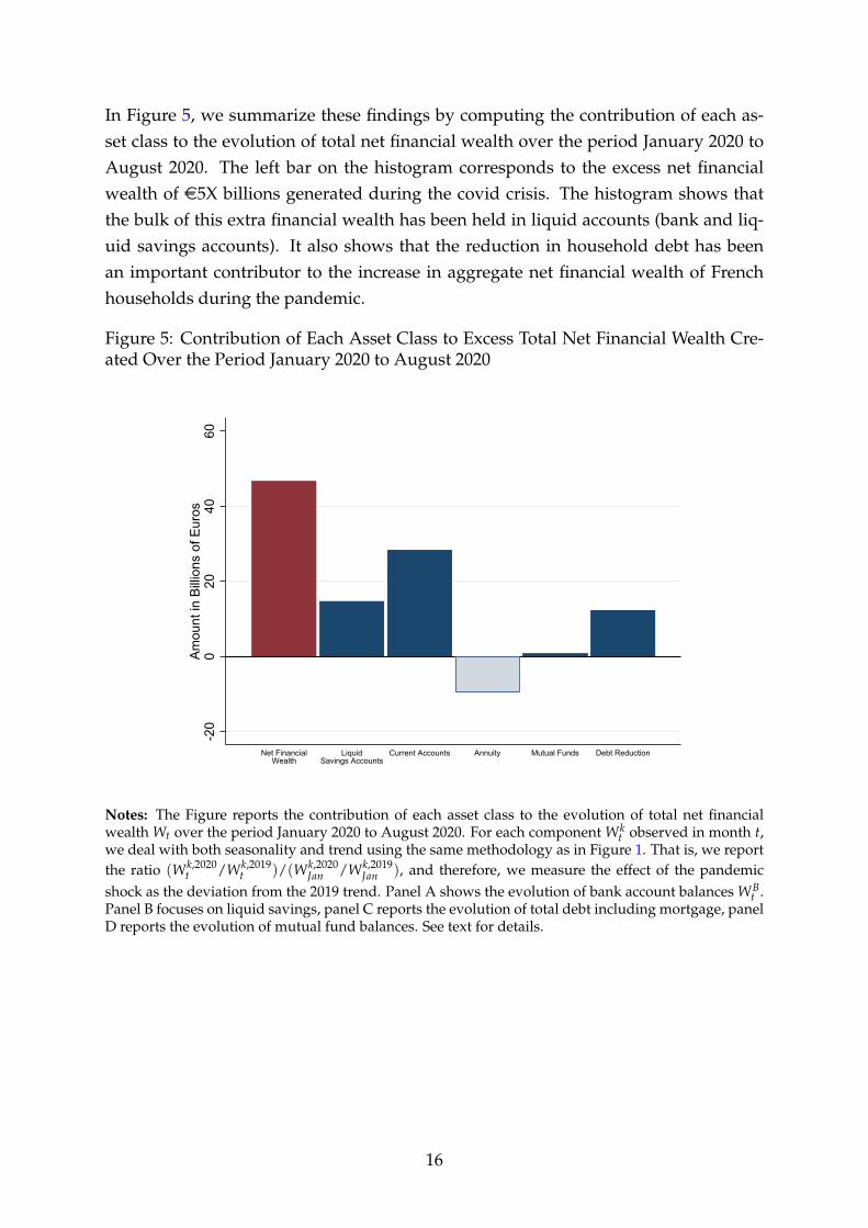
In Figure 5, we summarize these findings by computing the contribution of each as-set class to the evolution of total net financial wealth over the period January 2020 toAugust 2020. The left bar on the histogram corresponds to the excess net financialwealth of e5X billions generated during the covid crisis. The histogram shows thatthe bulk of this extra financial wealth has been held in liquid accounts (bank and liq-uid savings accounts). It also shows that the reduction in household debt has beenan important contributor to the increase in aggregate net financial wealth of Frenchhouseholds during the pandemic.

Figure 5: Contribution of Each Asset Class to Excess Total Net Financial Wealth Cre-ated Over the Period January 2020 to August 2020

-20

020

4060

Amou

nt in

Billi

ons

of E

uros

Net FinancialWealth

LiquidSavings Accounts

Current Accounts Annuity Mutual Funds Debt Reduction

Notes: The Figure reports the contribution of each asset class to the evolution of total net financialwealth Wt over the period January 2020 to August 2020. For each component Wk

t observed in month t,we deal with both seasonality and trend using the same methodology as in Figure 1. That is, we reportthe ratio (Wk,2020

t /Wk,2019t )/(Wk,2020

Jan /Wk,2019Jan ), and therefore, we measure the effect of the pandemic

shock as the deviation from the 2019 trend. Panel A shows the evolution of bank account balances WBt .

Panel B focuses on liquid savings, panel C reports the evolution of total debt including mortgage, panelD reports the evolution of mutual fund balances. See text for details.

16

4 Sectoral Heterogeneity

The richness of the CB data allows to document the large sectoral heterogeneity in theseverity of the covid shock.

4.1 Durables

We start by focusing on expenditures on durable goods. We define durable goodsas cars, motorcycles, home appliances, IT, furniture, and jewelry.8 The dynamics ofexpenditures on durables is in important signal regarding the underlying mechanismsdriving consumption dynamics. First, because, contrary to other goods or services,durables allow for intertemporal substitution. If the effect of the severe lockdown onconsumption was entirely driven by incapacitation effects, then we should see almostperfect intertemporal substitution. And durable expenditures would catch up postlockdown the losses made during the lockdown period. But durable consumptionis also an important signal regarding households’ expectations and is often stronglycorrelated with cyclical variation in economic activity, dipping strongly in recessions.The reason is that durables are an important means of consumption insurance againstthe expectations of future shocks. In the face of a future expected shock, one can usedurables to smooth consumption over time without having to incur new expenditures.

In Figure 6 below, we report in panel A the evolution of consumption expenditureson durables observed in the CB data following the same approach as in Figure 1 toaccount for trends and seasonality. The Figure shows that, after a very large declineduring the lockdown period, expenditures on durable goods have bounced back sig-nificantly right after lockdown and have been at a significantly higher level than in2019 ever since. Overall, this strong pattern of intertemporal reallocation of expendi-tures has enabled to recoup almost two thirds of the losses made during the lockdownperiod.

4.2 Hospitality

In panel B of Figure 6, we report, following a similar methodology, the evolution of ex-penditures in the hospitality sector, defined as sector codes "56", "90", "91" and "93" inthe French NAF classification. The patterns are markedly different compared to panelA. We see that the hospitality sector has been severely impacted by the lockdown, but

8This corresponds to the following sectors in the French NAF classification of sectors: "451","453","454", "474", "475", "4777".

17

did not experience a quick rebound after. Various administrative restrictions have re-mained in place in these sectors throughout the summer months, such that in annualterms it has lost 6.6% of annual expenditures since the end of the lockdown. Whenadded to the 13% annual expenditures already lost during the lockdown, this makesfor a historic and dramatic loss for 2020. Furthermore, hospitality expenditures havebeen declining since the end of August, as new cases started to rise in France, prompt-ing new administrative measures restricting consumption in these sectors.

4.3 Overall Heterogeneity Across Sectors

In Figure 7, we report the total annualized gains or losses in expenditures made byeach sector during the lockdown period, and the post-lockdown period. Results pro-vide a clear picture of the extreme heterogeneity in the severity of the shock acrosssectors, something that is quite unique compared to previous recessions. Overall, themajority of sectors was confronted with heavy losses in expenditures during the lock-down period, with only a few sectors doing better than in 2019. But interestingly, somesectors did compensate for these losses during the post-lockdown period with a sig-nificant rebound in expenditures (hardware stores, bookshops, etc). In contrast, somesectors continued to face extremely depressed expenditures (travel agencies, muse-ums, leisure centers, etc).

These results indicate that sectors face extremely heterogeneous prospects in termsof recovery, and different needs in terms of public policies. While some sectors haveexperienced temporary losses that did affect their liquidity but not their solvency inthe near future, others have faced permanent losses, and cannot anticipate a recoveryin terms of expenditures as long as the epidemic is not brought into control. Thesesectors are now facing extremely severe solvency issues, and their needs can only beaddressed via targeted sectoral policies.

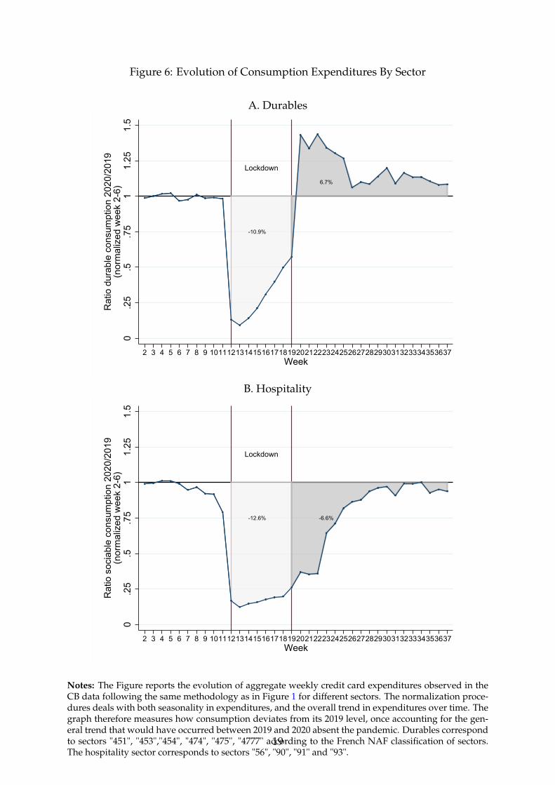
Figure 6: Evolution of Consumption Expenditures By Sector

A. Durables

Lockdown

-10.9%

6.7%

0.2

5.5

.75

11.

251.

5

Rat

io d

urab

le c

onsu

mpt

ion

2020

/201

9(n

orm

aliz

ed w

eek

2-6)

2 3 4 5 6 7 8 9 10111213141516171819202122232425262728293031323334353637Week

B. Hospitality

Lockdown

-12.6% -6.6%

0.2

5.5

.75

11.

251.

5

Rat

io s

ocia

ble

cons

umpt

ion

2020

/201

9(n

orm

aliz

ed w

eek

2-6)

2 3 4 5 6 7 8 9 10111213141516171819202122232425262728293031323334353637Week

Notes: The Figure reports the evolution of aggregate weekly credit card expenditures observed in theCB data following the same methodology as in Figure 1 for different sectors. The normalization proce-dures deals with both seasonality in expenditures, and the overall trend in expenditures over time. Thegraph therefore measures how consumption deviates from its 2019 level, once accounting for the gen-eral trend that would have occurred between 2019 and 2020 absent the pandemic. Durables correspondto sectors "451", "453","454", "474", "475", "4777" according to the French NAF classification of sectors.The hospitality sector corresponds to sectors "56", "90", "91" and "93".

19

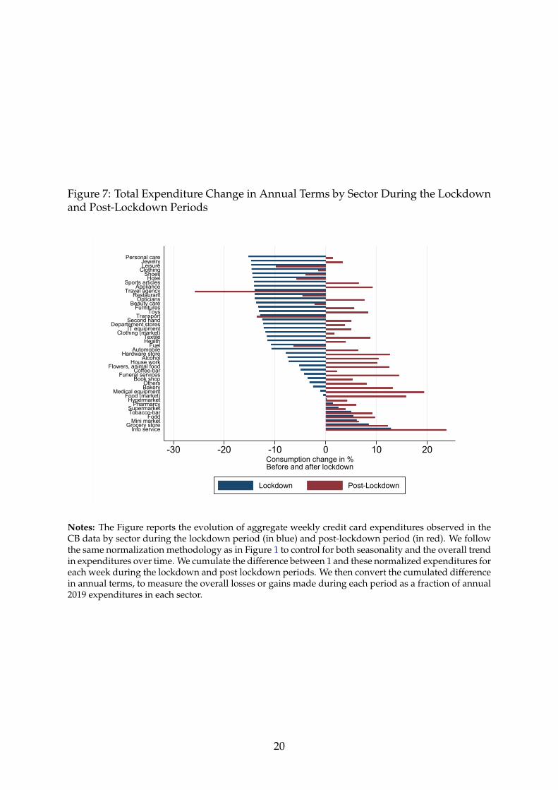
Figure 7: Total Expenditure Change in Annual Terms by Sector During the Lockdownand Post-Lockdown Periods

-30 -20 -10 0 10 20Consumption change in %Before and after lockdown

Info serviceGrocery store

Mini marketFodd

Tobacco-barSupermarket

PharmarcyHypermarket

Food (market)Medical equipment

BakeryOthers

Book shopFuneral services

Coffee-barFlowers, animal food

House workAlcohol

Hardware storeAutomobile

FuelHealthTextile

Clothing (market)IT equipment

Departement storesSecond hand

TransportToys

FurnituresBeauty care

OpticiansRestaurant

Travel agencyAppliance

Sports articlesHotel

ShoesClothingLeisureJewelry

Personal care

Lockdown Post-Lockdown

Notes: The Figure reports the evolution of aggregate weekly credit card expenditures observed in theCB data by sector during the lockdown period (in blue) and post-lockdown period (in red). We followthe same normalization methodology as in Figure 1 to control for both seasonality and the overall trendin expenditures over time. We cumulate the difference between 1 and these normalized expenditures foreach week during the lockdown and post lockdown periods. We then convert the cumulated differencein annual terms, to measure the overall losses or gains made during each period as a fraction of annual2019 expenditures in each sector.

20

5 Distributional Effects

We now turn to documenting heterogeneity in the responses of household consump-tion and savings to the crisis.

We first rank households in the CM panel according to their level of total expendi-tures in 2019. The CM data does not enable us yet to measure income flows precisely,and total consumption expenditures offer a good proxy for the standard of living ofa household pre-crisis.9 In Figure 8, we show in panel A the evolution of total con-sumption expenditures for different deciles of the distribution of pre-crisis expendi-tures. The graph shows that households in the bottom of the distribution of pre-crisisexpenditures experienced a smaller decrease in consumption during the lockdown,and a steeper rebound during the summer months. This finding of an overall largerdecline in consumption for richer households is reminiscent of the results in Chettyet al. [2020]. Note that their results are based on correlations between aggregate cardexpenditures and average income across zip codes, while our approach is based onindividual level variation in “income” levels.

Interpreting these differential consumption patterns is not straightforward. They mayfirst reflect differential variations in income or in income expectations. But they mayalso be due to differential perceptions regarding the risk of getting infected or severelyill, perceptions which may ultimately affect consumption behaviors. Finally, they mayalso simply reflect differential incapacitation in the face of the restrictions (e.g. lock-downs, etc) put in place by the the government: individuals have the top end of theincome distribution have usually a much larger share of their expenditures in sectorsthat have been shut down by the pandemic (travels, leisure, hospitality, etc.). It isimportant to understand which of these three main channels is driving consumptionpatterns to understand the distributional and welfare effects of the shock.

We start here by focusing on the role of income fluctuations and income expectations.Ideally, of course, we would like to be able to observe income, and its differential evo-lution across households. Unfortunately, we do not have (yet) a robust measure ofincome in the CM data. But by combining the patterns of evolution of consumptionand household financial wealth in the CM data, we can get a good indication of whathas happened to income, using households’ budget constraint identity (2). In panelB of Figure 8, we report the evolution of total gross savings, defined as the sum ofcurrent account balances, all liquid savings account balances, and of all mutual fundsbalances held in the bank, for different deciles of the distribution of 2019 total expen-ditures. Once again, we take care of trends and seasonality, using the same approachas in panel A. The graph shows that the crisis has caused a decline of about 2% of

9Total expenditures are defined as credit card transactions, check payments and cash withdrawals.

21

the total gross financial wealth for the “poorest” households (i.e. the bottom decilesof the distribution of pre-crisis expenditures). For households in the middle of thedistribution (5th decile), the crisis has created a small increase of about 1% of theirgross financial wealth, after an initial dip in March, due to the crash in asset prices.Interestingly, households at the top end of the distribution saw a larger dip than otherhouseholds in gross financial wealth in March, due to the larger fraction of their finan-cial wealth held in risky assets. But after this dip, the situation reversed: as of August,households in the 10th decile have experienced the largest increase in financial wealthin percentage terms (i.e. of about 4%). This rebound reflects both the rebound in assetprices following the initial crash, but also the steady flow of savings maintained bythese households since the start of the pandemic.

In panel C, we investigate the evolution of outstanding debt by deciles, and use thesame approach as before to detrend the data and take care of seasonality. We find thatpoorest households have seen a significant increase in their outstanding debt since thestart of the crisis. To the contrary, households at the top end of the distribution of pre-crisis expenditures have experienced a large decrease in the stock of their outstandingdebt, reflecting movements both at the intensive margin (debt repayments), and ex-tensive margin (fewer new debt contracts). Overall, the patterns reported in all threepanels of Figure 8 suggest that households at the bottom of the distribution, experi-enced both a decline in consumption and a decline in their net financial wealth. In-verting their budget constraint’s identity, this is direct evidence that they experienceda significant drop in income. Clearly, these households have been strongly affectedby the pandemic crisis, and, contrary to households at the top end of the distribution,have not been able to create a buffer of savings during the lockdown.

In Figure 9, we compute the contribution of each decile of pre-crisis expenditures tothe excess growth in net financial wealth over the period February to August 2020.The graph shows that the contribution of the poorest deciles was negative, as theyexperienced a decline in their net financial wealth. It also shows that more than 70%of thee45 billions in excess wealth have accrued to the top two deciles. And 55% aloneof this excess wealth went to the top decile. Given these top two deciles accounted fora little less than 45% of total net financial wealth before the pandemic, this suggeststhat the crisis has generated an increase in wealth inequality.

22

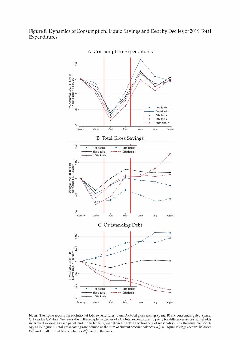
Figure 8: Dynamics of Consumption, Liquid Savings and Debt by Deciles of 2019 TotalExpenditures

A. Consumption Expenditures

.4.6

.81

1.2

Expe

nditu

res

Rat

io 2

020/

2019

Nor

mal

ized

in F

ebru

ary


1st decile2nd decile5th decile9th decile10th decile

B. Total Gross Savings

.96

.98

11.

021.

04

Savi

ngs

Rat

io 2

020/

2019

Nor

mal

ized

in F

ebru

ary


1st decile 2nd decile5th decile 9th decile10th decile

C. Outstanding Debt

.97

.98

.99

11.

011.

02

Deb

ts R

atio

202

0/20

19N

orm

aliz

ed in

Feb

ruar

y


1st decile 2nd decile5th decile 9th decile10th decile

Notes: The figure reports the evolution of total expenditures (panel A), total gross savings (panel B) and outstanding debt (panelC) from the CM data. We break down the sample by deciles of 2019 total expenditures to proxy for differences across householdsin terms of income. In each panel, and for each decile, we detrend the data and take care of seasonality using the same methodol-ogy as in Figure 1. Total gross savings are defined as the sum of current account balances WB

it , all liquid savings account balancesWS

it , and of all mutual funds balances WMit held in the bank.

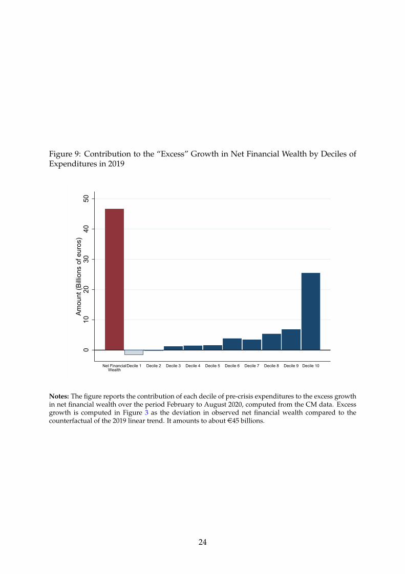
Figure 9: Contribution to the “Excess” Growth in Net Financial Wealth by Deciles ofExpenditures in 2019

010

2030

4050

Amou

nt (B

illion

s of

eur

os)

Net FinancialWealth

Decile 1 Decile 2 Decile 3 Decile 4 Decile 5 Decile 6 Decile 7 Decile 8 Decile 9 Decile 10

Notes: The figure reports the contribution of each decile of pre-crisis expenditures to the excess growthin net financial wealth over the period February to August 2020, computed from the CM data. Excessgrowth is computed in Figure 3 as the deviation in observed net financial wealth compared to thecounterfactual of the 2019 linear trend. It amounts to about e45 billions.

24

6 What Is Driving Consumption Dynamics?

We now investigate the role of three potential drivers of consumption dynamics dur-ing the pandemic. First, we focus on the role of income dynamics and income expec-tations. For this, we estimate marginal propensities to consume using the granularityof our data. Second, we explore the role of health risk. Finally, we measure the impactof restriction policies.

6.1 Income Dynamics & Marginal Propensities to Consume

To evaluate the role of income dynamics in explaining consumption and savings dy-namics, we focus on estimating marginal propensities to consume (MPC). MPCs mea-sure the sensitivity of consumption to income changes and are therefore importantto understand the aggregate demand effects of transfer and stimulus policies put inplace during the crisis. Furthermore, MPCs reveal households’ expectations about thefuture. The presence of strong precautionary saving motives for instance would trans-late into low MPCs, indicative that households prefer to use any extra income to builda buffer stock of savings in the face of uncertain income and employment dynam-ics. Finally and importantly, MPCs also help capturing the social value of transfers.Landais and Spinnewijn [forthcoming] show that, under particular assumptions, het-erogeneity in MPCs can identify heterogeneity in the underlying price of raising anextra e of consumption. As a result, while consumption dynamics alone is a poorguide to evaluate the welfare consequences of a shock, heterogeneity in MPCs is keyto measure the differential welfare impacts of such shocks, and determine the redis-tributive and social value of transfers.

Identifying MPCs To identify MPCs, we exploit eligibility criteria for a specific wel-fare transfer called the “Allocation de Rentree Scolaire” (ARS). This welfare transfer isa one-time payment made in August, just before the start of the school year, to familieswith children above 6 years old. The transfer is means-tested. This year, the regularamount was topped-up by an extra e100 payment, so that eligible families receivede470 per child for children between six and ten years old. We focus on households inthe CM panel with one or two children meeting the means-test requirement to receivethe payments. We then create two groups from this subsample. The treatment groupcomprises households with just one child, whose age is between 6 and 10 years old,as well as families with two children, with one of them being between 6 and 10 yearsold and the other between 3 and 5 years old. The control group is made of householdswith just one child, whose age is between 3 and 5 years old, as well as families with

25

two children, both of them being between 3 and 5 years old. The treatment group re-ceives a e470 ARS payment on August 18th, while the control group does not receiveany payment on this date. Identification relies on a standard diff-in-diff assumptionof parallel trends.

Figure 10 shows the difference in average weekly expenditures between householdsin the treatment and control group, normalized to zero in week 33. The differencewas extremely stable in the weeks preceding the ARS payment, lending credibility toour diff-in-diff identifying assumption. We see a sudden and sharp increase in con-sumption expenditures by households in the treated group in week 34, just after theyreceive the ARS welfare payment. When scaled by the value of the transfer (i.e. e470),this sharp increase in expenditures translates into a MPC estimate of .15 for the firsttwo weeks. These findings are consistent with estimated expenditures responses toCARES Act stimulus payments in the US, from Chetty et al. [2020] (who use aggre-gate card transaction data), as well as from Baker et al. [2020] and Karger and Rajan[2020] who use individual transaction data. Note that the estimated MPCs from thelatter two studies are slightly higher (around .2 to .25) but they both rely on samplesprimarily made of lower-income individuals (compared to the population eligible toARS).

In Figure 11, we show the presence of strong heterogeneity in estimated MPCs. Wesplit the estimation sample by quartiles of liquid savings, defined as the sum of cur-rent account balances WB

it , all liquid savings account balances WSit , and of all mutual

funds balances WMit . The graph shows that estimated MPCs are three times larger for

households in the bottom quartile of liquid savings compared to households in the topquartile.

26

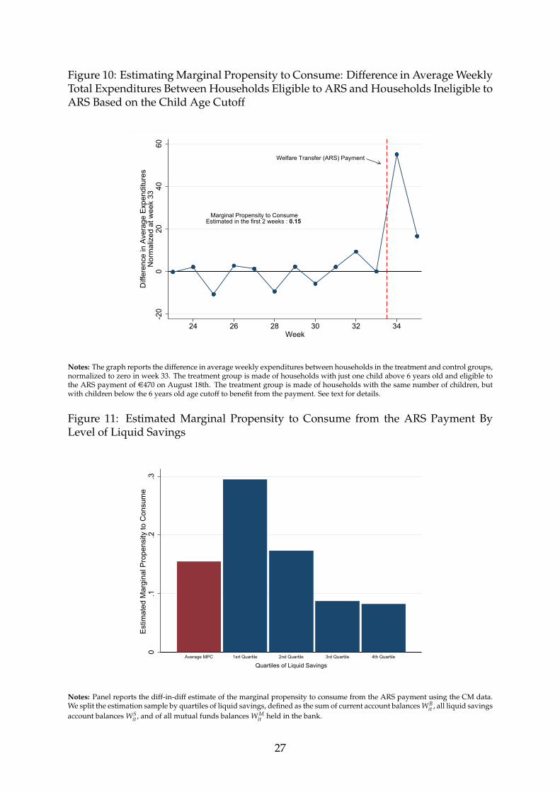
Figure 10: Estimating Marginal Propensity to Consume: Difference in Average WeeklyTotal Expenditures Between Households Eligible to ARS and Households Ineligible toARS Based on the Child Age Cutoff

Marginal Propensity to ConsumeEstimated in the first 2 weeks : 0.15

Welfare Transfer (ARS) Payment-2

00

2040

60

Diff

eren

ce in

Ave

rage

Exp

endi

ture

sN

orm

aliz

ed a

t wee

k 33

24 26 28 30 32 34Week

Notes: The graph reports the difference in average weekly expenditures between households in the treatment and control groups,normalized to zero in week 33. The treatment group is made of households with just one child above 6 years old and eligible tothe ARS payment of e470 on August 18th. The treatment group is made of households with the same number of children, butwith children below the 6 years old age cutoff to benefit from the payment. See text for details.

Figure 11: Estimated Marginal Propensity to Consume from the ARS Payment ByLevel of Liquid Savings

0.1

.2.3

Estim

ated

Mar

gina

l Pro

pens

ity to

Con

sum

e

Average MPC 1srt Quartile 2nd Quartile 3rd Quartile 4th Quartile

Quartiles of Liquid Savings

Notes: Panel reports the diff-in-diff estimate of the marginal propensity to consume from the ARS payment using the CM data.We split the estimation sample by quartiles of liquid savings, defined as the sum of current account balances WB

it , all liquid savingsaccount balances WS

it , and of all mutual funds balances WMit held in the bank.

27

6.2 Health Risk

Time Series & Cross-sectional Geographical Evidence How much is consumptiondynamics impacted by the increased health risk that people face due to the pandemic?The first natural approach is to look at time series and cross-sectional variation in theseverity of the epidemic, and use this variation to estimate correlation with consump-tion expenditures. In Figure 12, we plot the evolution of ICU admissions in Franceagainst the evolution of aggregate daily card transactions in the CB data, using a 7-daymoving average.10 The graph shows the presence of a strong correlation in the time se-ries between virus dynamics and aggregate consumption behaviors. In particular, thegraph shows that aggregate consumption has started to falter since mid-September, asthe second wave of the epidemic was gaining strength in France. Cross-sectional vari-ation confirms the presence of a strong correlation between virus spread and aggregateconsumption: in panel B, we display an binscatter of aggregate log CB consumption inSeptember 2020 (relative to log aggregate CB consumption in September 2019) by “de-partement”, against the number of average daily new confirmed cases in September by“departement”.11 The binscatter is residualized on a series of controls for observablecharacteristics at the departement level, including population size, density, occupa-tional structure of the workforce, age structure of the population. The graph indicatesclearly that departements in which the number of cases is the highest in September arealso facing the lowest level of aggregate card transactions.

Evidence from Figure 12 clearly indicates that the steady and quick rebound of aggre-gate consumption observed in France during the Summer months is now at risk, andthere is a clear slowdown of expenditures since mid-September, as the second waveis looming. However, it is hard to interpret the correlations from Figure 12 as directevidence of a causal link between health risk and consumption dynamics, as there is astrong correlation in the time series and in the cross-section between the severity of theepidemic and restriction policies. To counter the rapid spread of the virus, the Frenchgovernment has indeed strengthened restrictions since early September, and enabledlocal jurisdictions to take targeted restrictions and lockdown measures.

10ICU admissions come from the official data series released by the French government on the “SantePublique France” web portal.

11A “departement” is a French political jurisdiction. There are about 100 “departements” in France.Numbers of daily new confirmed cases by departement come from the “Sante Publique France” webportal.

28

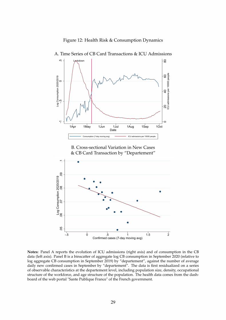
Figure 12: Health Risk & Consumption Dynamics

A. Time Series of CB Card Transactions & ICU AdmissionsLockdown

020

4060

80IC

U a

dmis

sion

s pe

r 100

00 p

eopl

e

-1-.5

0.5

Log

Con

sum

ptio

n 20

20/2

019

1Apr 1May 1Jun 1Jul 1Aug 1Sep 1OctDate

Consumption (7-day moving avg) ICU admissions per 10000 people

B. Cross-sectional Variation in New Cases& CB Card Transaction by “Departement”

.05

.06

.07

.08

.09

.1Lo

g C

onsu

mpt

ion

2020

/201

9

-.5 0 .5 1 1.5 2Confirmed cases (7-day moving avg)

Notes: Panel A reports the evolution of ICU admissions (right axis) and of consumption in the CBdata (left axis). Panel B is a binscatter of aggregate log CB consumption in September 2020 (relative tolog aggregate CB consumption in September 2019) by “departement”, against the number of averagedaily new confirmed cases in September by “departement”. The data is first residualized on a seriesof observable characteristics at the departement level, including population size, density, occupationalstructure of the workforce, and age structure of the population. The health data comes from the dash-board of the web portal "Sante Publique France" of the French government.

29

Age Variation To try to identify the causal relationship between health risk and con-sumption dynamics, we examine heterogeneity in patterns of consumption across agegroups. There has not been any age-specific restriction policies put in place during thepandemic, that may confound the correlation observed between age and consump-tion. Furthermore, there is a clear gradient in health risk by age, as older people aremore likely to die from the new coronavirus. To identify first how risk perceptionsvaried by age, and correlate with actual risk, we use elicited risk perceptions of dyingfrom the coronavirus from the DataCovid survey, which was conducted in June on arandom representative sample of 5,000 individuals. Three insights emerge from thispanel. First, the overall average elicited risk of dying strongly overstates the true ac-tual risk of dying from the virus. Second, we find a strong gradient in elicited risk,with older people clearly perceiving their higher likelihood of dying from the virus.But thirdly, the gradient is smaller than the actual gradient in true risk. Epidemiolog-ical studies suggest that individuals above 65 years old are 4 to 5 times more likely todie from the virus than individuals below 40 years old. In the survey, we see that thisgradient is only of about 2: older individuals believe on average to be about 2 timesonly more likely to die than 18-34 years old. This indicates that there is strong upwardbias in risk perception in younger individuals, compared to older individuals.

In panel B, we investigate to what extent these differential percpetions translate intoconsumption dynamics. We use the CM data and plot the evolution of total expendi-tures for three age groups. We see that during the lockdown period, consumption ofthe elderly decreased significantly more than that of younger age groups. But interest-ingly, we see that as soon as the lockdown ended, consumption patterns reverted backto their 2019 levels for all age groups, without significant differences in consumptiondynamics during the summer months. Note that if we break down consumption bysectors, we do find that the consumption structures of the elderly changed comparedto younger age groups: the elderly are less likely to engage in consumption involvingsocial interactions (restaurants, etc). Yet, these differences in structure do not seem toimpact aggregate consumption levels, suggesting the presence of strong substitutionacross consumption types.

These results suggest that health risk perceptions may have been less consequentialthan restriction policies to explain, in the French context, the strong correlation be-tween the dynamics of the epidemic, and that of consumption. To confirm this, wenow turn to identifying the effect of restriction policies more directly.

30

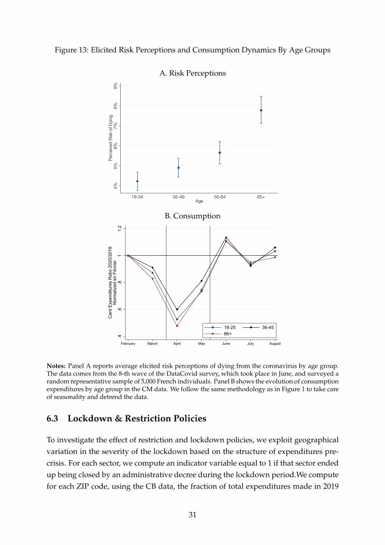
Figure 13: Elicited Risk Perceptions and Consumption Dynamics By Age Groups

A. Risk Perceptions

4%

5%

6%

7%

8%

9%

Perc

eiv

ed

Ris

k of D

ying

18-34 35-49 50-64 65+Age

B. Consumption

.4.6

.81

1.2

Car

d Ex

pend

iture

s R

atio

202

0/20

19N

orm

aliz

ed e

n Fé

vrie

r


18-25 36-4566+

Notes: Panel A reports average elicited risk perceptions of dying from the coronavirus by age group.The data comes from the 8-th wave of the DataCovid survey, which took place in June, and surveyed arandom representative sample of 5,000 French individuals. Panel B shows the evolution of consumptionexpenditures by age group in the CM data. We follow the same methodology as in Figure 1 to take careof seasonality and detrend the data.

6.3 Lockdown & Restriction Policies

To investigate the effect of restriction and lockdown policies, we exploit geographicalvariation in the severity of the lockdown based on the structure of expenditures pre-crisis. For each sector, we compute an indicator variable equal to 1 if that sector endedup being closed by an administrative decree during the lockdown period.We computefor each ZIP code, using the CB data, the fraction of total expenditures made in 2019

31

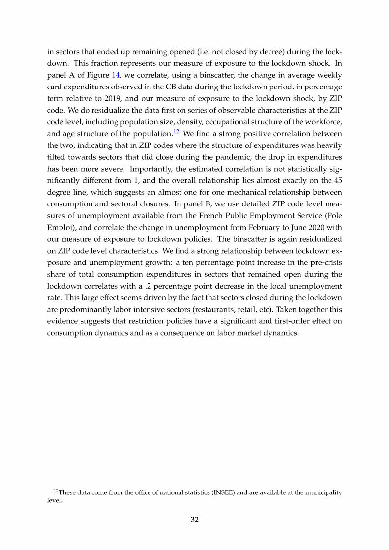
in sectors that ended up remaining opened (i.e. not closed by decree) during the lock-down. This fraction represents our measure of exposure to the lockdown shock. Inpanel A of Figure 14, we correlate, using a binscatter, the change in average weeklycard expenditures observed in the CB data during the lockdown period, in percentageterm relative to 2019, and our measure of exposure to the lockdown shock, by ZIPcode. We do residualize the data first on series of observable characteristics at the ZIPcode level, including population size, density, occupational structure of the workforce,and age structure of the population.12 We find a strong positive correlation betweenthe two, indicating that in ZIP codes where the structure of expenditures was heavilytilted towards sectors that did close during the pandemic, the drop in expenditureshas been more severe. Importantly, the estimated correlation is not statistically sig-nificantly different from 1, and the overall relationship lies almost exactly on the 45degree line, which suggests an almost one for one mechanical relationship betweenconsumption and sectoral closures. In panel B, we use detailed ZIP code level mea-sures of unemployment available from the French Public Employment Service (PoleEmploi), and correlate the change in unemployment from February to June 2020 withour measure of exposure to lockdown policies. The binscatter is again residualizedon ZIP code level characteristics. We find a strong relationship between lockdown ex-posure and unemployment growth: a ten percentage point increase in the pre-crisisshare of total consumption expenditures in sectors that remained open during thelockdown correlates with a .2 percentage point decrease in the local unemploymentrate. This large effect seems driven by the fact that sectors closed during the lockdownare predominantly labor intensive sectors (restaurants, retail, etc). Taken together thisevidence suggests that restriction policies have a significant and first-order effect onconsumption dynamics and as a consequence on labor market dynamics.

12These data come from the office of national statistics (INSEE) and are available at the municipalitylevel.

32

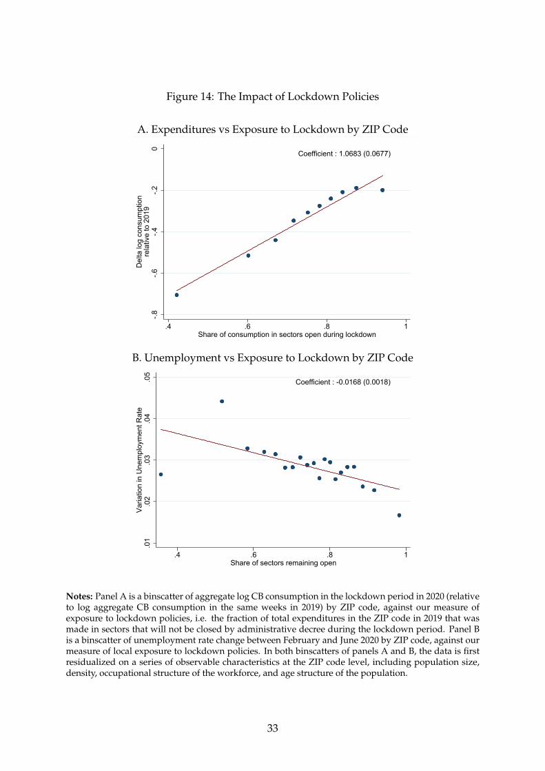
Figure 14: The Impact of Lockdown Policies

A. Expenditures vs Exposure to Lockdown by ZIP Code

-.8-.6

-.4-.2

0

Del

ta lo

g co

nsum

ptio

nre

lativ

e to

201

9

.4 .6 .8 1Share of consumption in sectors open during lockdown

Coefficient : 1.0683 (0.0677)

B. Unemployment vs Exposure to Lockdown by ZIP Code

.01

.02

.03

.04

.05

Varia

tion

in U

nem

ploy

men

t Rat

e

.4 .6 .8 1Share of sectors remaining open

Coefficient : -0.0168 (0.0018)

Notes: Panel A is a binscatter of aggregate log CB consumption in the lockdown period in 2020 (relativeto log aggregate CB consumption in the same weeks in 2019) by ZIP code, against our measure ofexposure to lockdown policies, i.e. the fraction of total expenditures in the ZIP code in 2019 that wasmade in sectors that will not be closed by administrative decree during the lockdown period. Panel Bis a binscatter of unemployment rate change between February and June 2020 by ZIP code, against ourmeasure of local exposure to lockdown policies. In both binscatters of panels A and B, the data is firstresidualized on a series of observable characteristics at the ZIP code level, including population size,density, occupational structure of the workforce, and age structure of the population.

33

References

Andersen, Asger, Emil Toft Hansen, Niels Johannesen, and Adam Sheridan. 2020.“Consumer Responses to the COVID-19 Crisis: Evidence from Bank Account Trans-action Data.” C.E.P.R. Discussion Papers CEPR Discussion Papers 14809.

Baker, Scott R, Robert A Farrokhnia, Steffen Meyer, Michaela Pagel, and Constan-tine Yannelis. 2020. “How Does Household Spending Respond to an Epidemic?Consumption during the 2020 COVID-19 Pandemic.” The Review of Asset PricingStudies. raaa009.

Bounie, David, Youssouf Camara, and John W. Galbraith. 2020. “Consumers’ Mobil-ity, Expenditure and Online-Offline Substitution Response to COVID-19: Evidencefrom French Transaction Data.” CIRANO CIRANO Working Papers 2020s-28.

Carvalho, V, Juan R. Garcia, S. Hansen, A. Ortiz, T. Rodrigo, and J. V. R. More. 2020.“Tracking the COVID-19 Crisis with High-Resolution Transaction Data.” Facultyof Economics, University of Cambridge Cambridge Working Papers in Economics2030.

Chetty, Raj, John N Friedman, Nathaniel Hendren, Michael Stepner, and The Op-portunity Insights Team. 2020. “How Did COVID-19 and Stabilization Policies Af-fect Spending and Employment? A New Real-Time Economic Tracker Based onPrivate Sector Data.” National Bureau of Economic Research Working Paper 27431.

Eika, Lasse, Magne Mogstad, and Ola L. Vestad. 2020. “What can we learn abouthousehold consumption expenditure from data on income and assets?” Journal ofPublic Economics, 189: 104163.

Hacioglu, Sinem, Diego Känzig, and Paolo Surico. 2020. “the distributional impactof the pandemic.” CEPR Discussion Papers, 15101.

Karger, Ezra, and Aastha Rajan. 2020. “Heterogeneity in the Marginal Propensity toConsume: Evidence from Covid-19 Stimulus Payments.” Federal Reserve Bank ofChicago Working Paper Series WP 2020-15.

Kolsrud, Jonas, Camille Landais, and Johannes Spinnewijn. 2020. “The value of reg-istry data for consumption analysis: An application to health shocks.” Journal ofPublic Economics, 189: 104088.

Landais, Camille, and Johannes Spinnewijn. forthcoming. “The Value of Unemploy-ment Insurance.” The Review of Economic Studies.

34

APPENDIX

Data

Groupement des Cartes Bancaires CB Le Groupement des Cartes Bancaires CB,Groupement d’Intérêt Economique qui définit les modalités de fonctionnement duschéma de paiement par carte CB (physique ou dématérialisée dans le mobile) a égale-ment contribué Ã cette étude par la fourniture de ses données (agrégées) et par la pos-sibilité de solliciter des traitements sur des données individuelles anonymisées dansun espace strictement sécurisé et dans le cadre de son partenariat avec la Chaire Fi-nance Digitale. “Le partenariat entre CB et le monde académique va permettre dedévelopper de nouvelles filières de compétence. Il reflète aussi la démarche citoyenneet responsable de CB, qui a pour volonté de servir l’intérêt général et favoriser l’inclusionsociale et sociétale”, déclare Philippe Laulanie, Directeur Général de CB.

Crédit Mutuel Alliance Fédérale Première banque à adopter le statut d’entreprise àmission, Crédit Mutuel Alliance Fédérale a contribué à cette étude par la fourniture dedonnées dans le cadre des missions qu’il s’est fixé :

• contribuer au bien commun en oeuvrant pour une société plus juste et plusdurable : en participant à l’information économique, Crédit Mutuel AllianceFédérale réaffirme sa volonté de contribuer au débat démocratique ;

• protéger l’intimité numérique et la vie privée de chacun : Crédit Mutuel AllianceFédérale veille à la protection absolue des données de ses clients. Toutes lesanalyses réalisées dans le cadre de cette étude ont été effectuées sur des donnéesnon identifiantes (pas de nom, prénom ou adresse de résidence) sur les seulssystèmes d’information sécurisés du Crédit Mutuel en France.

Representativeness of CM Sample

35

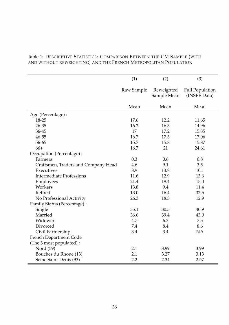
Table 1: DESCRIPTIVE STATISTICS: COMPARISON BETWEEN THE CM SAMPLE (WITHAND WITHOUT REWEIGHTING) AND THE FRENCH METROPOLITAN POPULATION

(1) (2) (3)

Raw Sample Reweighted Full PopulationSample Mean (INSEE Data)

Mean Mean Mean

Age (Percentage) :18-25 17.6 12.2 11.6526-35 16.2 16.3 14.9636-45 17 17.2 15.8546-55 16.7 17.3 17.0656-65 15.7 15.8 15.8766+ 16.7 21 24.61

Occupation (Percentage) :Farmers 0.3 0.6 0.8Craftsmen, Traders and Company Head 4.6 9.1 3.5Executives 8.9 13.8 10.1Intermediate Professions 11.6 12.9 13.6Employees 21.4 19.4 15.0Workers 13.8 9.4 11.4Retired 13.0 16.4 32.5No Professional Activity 26.3 18.3 12.9

Family Status (Percentage) :Single 35.1 30.5 40.9Married 36.6 39.4 43.0Widower 4.7 6.3 7.5Divorced 7.4 8.4 8.6Civil Partnership 3.4 3.4 NA

French Department Code(The 3 most populated) :

Nord (59) 2.1 3.99 3.99Bouches du Rhone (13) 2.1 3.27 3.13Seine Saint-Denis (93) 2.2 2.34 2.57

36

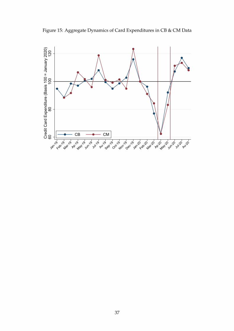
Figure 15: Aggregate Dynamics of Card Expenditures in CB & CM Data

6080

100

120

Cre

dit C

ard

Expe

nditu

re (B

asis

100

= J

anua

ry 2

020)

Jan-1

9

Feb-19

Mar-19

Ap-19

May-19

Jun-1

9Ju

l-19

Au-19

Sep-19

Oct-19

Nov-19

Dec-19

Jan-2

0

Feb-20

Mar-20

Ap-20

May-20

Jun-2

0Ju

l-20

Au-20

CB CM

37

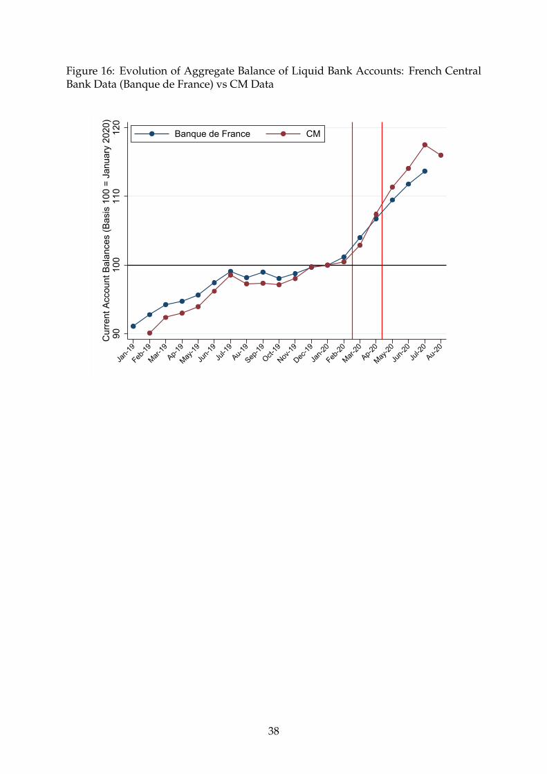
Figure 16: Evolution of Aggregate Balance of Liquid Bank Accounts: French CentralBank Data (Banque de France) vs CM Data

9010

011

012

0C

urre

nt A

ccou

nt B

alan

ces

(Bas

is 1

00 =

Jan

uary

202

0)

Jan-1

9

Feb-19

Mar-19

Ap-19

May-19

Jun-1

9Ju

l-19

Au-19

Sep-19

Oct-19

Nov-19

Dec-19

Jan-2

0

Feb-20

Mar-20

Ap-20

May-20

Jun-2

0Ju

l-20

Au-20

Banque de France CM

38

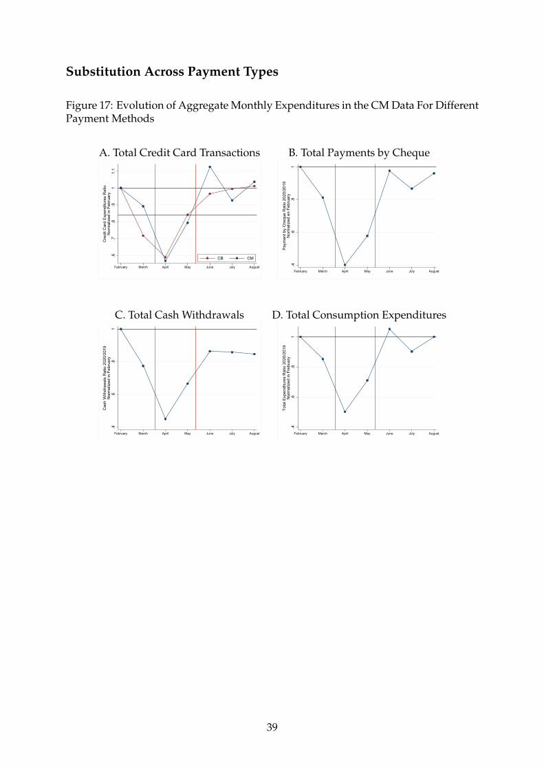
Substitution Across Payment Types

Figure 17: Evolution of Aggregate Monthly Expenditures in the CM Data For DifferentPayment Methods

A. Total Credit Card Transactions B. Total Payments by Cheque

.6.7

.8.9

11.

1

Cre

dit C

ard

Expe

nditu

res

Rat

ioN

orm

aliz

ed in

Feb

ruar

y


CB CM

.4.6

.81

Paym

ent b

y C

hequ

e R

atio

202

0/20

19N

orm

aliz

ed e

n Fe

brua

ry


C. Total Cash Withdrawals D. Total Consumption Expenditures

.4.6

.81

Cas

h W

ithdr

awal

s R

atio

202

0/20

19N

orm

aliz

ed in

Feb

ruar

y


.4.6

.81

Tota

l Exp

endi

ture

s R

atio

202

0/20

19N

orm

aliz

ed in

Fre

buar

y


39

Dynamiques de consommation dans la crise

Documents

Transcript of Dynamiques de consommation dans la crise