A Riemannian Approach to

Anisotropic Filtering of Tensor Fields

C.A. Castano-Moragaa,b, C. Lengleta, R. Derichea and

J. Ruiz-Alzolab

aI.N.R.I.A., Projet Odyssee, 2004 route des lucioles, 06902 Sophia-Antipolis, France.

bCenter for Technology in Medicine, Signals and Communications Department, Building

B, University of Las Palmas de Gran Canaria. Campus de Tafira s/n. 35017 Tafira, Spain.

Abstract

Tensors are nowadays an increasing research domain in different areas, especially in image

processing, motivated for example by DT-MRI (Diffusion Tensor Magnetic Resonance

Imaging). Up to now, algorithms and tools developed to deal with tensors were founded

on the assumption of a matrix vector space with the constraint of remaining symmetric

positive definite matrices. On the contrary, our approach is grounded on the theoretically

well-founded differential geometrical properties of the space of multivariate normal

distributions, where it is possible to define an affine-invariant Riemannian metric and

express statistics on the manifold of symmetric positive definite matrices. In this paper,

we focus on the contribution of these tools to the anisotropic filtering and regularization of

tensor fields. To validate our approach we present promising results on both, synthetic and

real DT-MRI data.

Key words: Differential geometry, Riemannian manifold, Geodesic distance, DT-MRI,

Tensor fields, Regularization, Anisotropic filtering, Nonlinear diffusion.

Preprint submitted to Elsevier Science 2 March 2006

1 Introduction

DT-MRI (Diffusion Tensor Magnetic Resonance Imaging) is a relatively new

medical imaging modality [3,34] from which a great deal of research on tensors

has stemmed. But this is not the only domain where tensors arise. Image structure

analysis through the Local Structure Tensor [4], stress and strain analysis of

materials [5] or electromagnetism [35] are other examples. Whatever domain we

are referring to, working with these tensor fields may require some regularization to

reduce the noise arising, for instance, from the acquisition process. Regularization

and filtering schemes of tensor fields are widely studied in the literature, especially

in the domain of DT-MRI. As an example, [29] deals with the problem of

regularizing noisy fields of diffusion tensors, considered as symmetric and positive

definiten×n matrices, through a PDE-based scheme and a spectral decomposition.

A complementary work is that presented in [11] which provides a geometric

interpretation of constrained flows for matrix-valued functions. This yields, through

the use of exponential maps, suitable numerical schemes that are also constraints

preserving. Another approach presented in [33] provides a generalization of

anisotropic and nonlinear diffusion process to matrix-valued data. More recently,

[12] proposes a scheme, based on variational methods, restoring the main direction

of the tensors and using the resulting direction to regularize the eigenvalues by an

anisotropic diffusion process. However, tensor eigenvalues tend to regularize faster

than the associated eigenvectors. This phenomenon is known as theeigenvalue

swelling effect for long regularization time, as shown in [30], while noise removal

Email addresses:ccasmor@ctm.ulpgc.es (C.A. Castano-Moraga ),

Christophe.Lenglet@sohpia.inria.fr (C. Lenglet),

Rachid.Deriche@sophia.inria.fr (R. Deriche),jruiz@ctm.ulpgc.es (J.

Ruiz-Alzola).

2

is not quite significant for short time regularization.

Other works try to couple the regularization with the tensors estimation process

from diffusion-weighted images. For example, [31] presents a constrained

variational principle which involves the minimization of a regularization term,

based onLp norms and subject to a nonlinear constraint on the data to obtain

positive definite tensors.

In this paper, we will rely on [17,18] where the authors proposed to use the

differential geometrical properties of the space of multivariate normal distributions

to define statistics on diffusion tensors, i.e. covariance matrices. This work is based

on the information geometry derived from the Fisher information, as proposed for

instance by Amari in [1].

Independently, other recent papers also addressed the issue of defining statistical

quantities and filtering tools for tensor fields. [14] first analyzes the space of

symmetric, positive definite matrices from a Lie groups perspective and shows

that this space does not form a vector space but can be regarded as a Riemannian

symmetric space. The authors used these ideas to develop efficient and elegant

methods for computing statistics and modes of variation of diffusion tensor data

in this non linear space.

More recently, and in parallel to our work initiated earlier in [17], [25] developed

also a nice and elegant computational framework for tensor processing with a

particular emphasize on interpolation, regularization and restoration of noisy tensor

fields.

Adding to these works where similar tools have been developed in order to study

the statistical variability of diffusion tensor images, one can also refer to the original

point of view based on the information geometry recently developed in [18]. It is

thus very interesting to note that comparable results were obtained through different

means while studying the statistical variability of diffusion tensor images. In our

3

work, we use the mathematical framework, developed in [28] and used in [18] to

take into account the particular geometry of the set of symmetric, positive definite

matrices in the smoothing process. We introduce an anisotropic filtering algorithm

controlled by the magnitude of the spatial gradient of the tensor field. On the

contrary of [14], where a statistical analysis of diffusion tensors was proposed but

without addressing the problem of smoothing, or [25], where the regularization

task was addressed with a PDE point of view, our smoothing method, developed

in parallel to [25] and based on our previous work developed earlier in [17], only

relies on simple and local anisotropic averaging. Adding to that, our method is

favorably compared to a state-of-the-art approach [33]. A detailed analysis of the

performances of our approach is performed and qualitative and quantitative results

obtained on noisy and synthetic data show that our approach outperforms the one

proposed in [33]. The emphasize of this article is not on the derivation of the

Riemannian framework, which we developed earlier in [17,18], but rather on its

clear and efficient application to solve the important problem of anisotropically

smoothing a set of noisy tensor data using the right concepts and tools, extending

our previous PDE based approaches in [29].

Section 2 recalls basic facts on the differential geometry of the space of multivariate

normal distributions and section 3 shows how they can be used to compute local

averages and spatial gradient of diffusion tensor images. Section 4 introduces the

filtering process. Finally, section 5 presents and discusses numerical experiments.

We will show that our Riemannian anisotropic filtering method yields better results

on both synthetic and real DT-MRI datasets when compared to other approaches

such as the nonlinear diffusion proposed in [33].

4

2 Geometry of the Space of Multivariate Normal Distributions

We hereafter review the necessary material related to the Riemannian geometry

of the multivariate normal model. As in [18], we consider the family of three-

dimensional normal distributions with 0-mean as the 6-dimensional parameter

space of variances and covariances. We identify it withS+(3), the set of 3× 3

real symmetric positive definite matrices, e.g. covariance matrices. Following the

work by Rao [27] and Burbea-Rao [7], where a Riemannian metric was introduced

for S+(3) in terms of the Fisher information matrix, it is possible to define notions

such as the geodesic distance, the curvature, the mean, and the covariance matrix for

elements ofS+(3). The basis of the tangent spaceTΣS+(3) = SΣ(3) atΣ ∈ S+(3) is

taken to be as in [28] and denoted byEi , i = 1, ...,6. The local coordinates are given

by θ1 = Σ11, θ2 = Σ12, ..., θ6 = Σ33. The fundamental mathematical tools needed to

derive our numerical schemes were detailed in [28], [8], [13], [9], [15] and [22].

Without employing the information geometry associated to the Fisher information

matrix but instead, identifyingS+(3) with the quotient spaceGL+(3)/S O(3), (with

GL+(3) the general linear group of positive definite 3× 3 matrices andS O(3) the

special orthogonal group of 3× 3 matrices), other works such as [14] and [25]

recently used similar ideas to derive statistical or filtering tools on tensors fields.

By extending the symmetry group to SL(3), [20] studied a slightly different metric

which turns out to exhibit an additional term in one direction. This extension was

also recently formulated by [21] in terms of a weighted Fisher information matrix.

They also generalized this approach to a wider class of elliptical densities. The

metric tensor forS+(3), derived from the Fisher information matrix is given by the

following theorem, which is proved in [28]:

Theorem 1 The Riemannian metric for the space S+(3) of multivariate normal

5

distributions with zero mean is given,∀Σ ∈ S+(3) by:

gi j = g(Ei ,E j) = 〈Ei ,E j〉Σ =12

tr(Σ−1EiΣ

−1E j

)i, j = 1, ...,6 (1)

In practice, this means that for any tangent vectorsA, B, their inner product relative

to Σ is 〈A, B〉Σ = 12tr(Σ−1AΣ−1B

). We recall that, ifΣ : t 7→ Σ(t) ∈ S+(3), ∀t ∈

[t1, t2] ⊂ R denotes a curve segment inS+(3) between two normal distributions

parameterized by the matricesΣ1 andΣ2, its length is expressed as:

LΣ(Σ1,Σ2) =∫ t2

t1

6∑i, j=1

gi j (Σ(t))dθi(t)

dt

dθ j(t)

dt

1/2

dt (2)

As stated for example in [22], the geodesic starting fromΣ(t1) ∈ S+(3) in the

directionV = Σ(t1) of the tangent spaceTS+(3) = S(3), is given by the exponential

map:

Σ(t) = Σ(t1)1/2 exp

((t − t1)Σ(t1)

−1/2VΣ(t1)−1/2)Σ(t1)

1/2∀t ∈ [t1, t2] (3)

We recall that the geodesic distanceD between any two elementsΣ1 andΣ2 is the

length of the minimizing geodesic betweenΣ1 andΣ2:

D(Σ1,Σ2) = infΣLΣ(Σ1,Σ2) : Σ1 = Σ(t1),Σ2 = Σ(t2)

It is given by the following theorem, whose original proof is available in an

appendix of [2] but different versions can also be found in [28] and [15].

Theorem 2 (S.T. Jensen, 1976)Consider the family of multivariate normal

distributions with common mean vector but different covariance matrices. The

geodesic distance between two members of the family with covariance matrices

Σ1 andΣ2 is given by

D(Σ1,Σ2) =

√12

tr(log2(Σ−1/21 Σ2Σ

−1/21

))=

√√12

3∑i=1

log2(ηi) (4)

6

whereηi denote the3 eigenvalues of the matrixΣ−1/21 Σ2Σ

−1/21 .

3 Local Average and Spatial Gradient of Diffusion Tensor Fields

Now, we can recall how the local average and spatial gradient of a diffusion tensor

image can be computed.

3.1 Intrinsic mean

To estimate the intrinsic mean distribution of a set of zero-mean multivariate

normal distributions we resort to a gradient descent algorithm. As proposed in

[18], we use the classical definition of the Riemannian center of mass and the

geodesic equations to derive a manifold constrained numerical integrator and thus

ensure that each step forward of the gradient descent stays within the spaceS+(3).

The normal distribution parametrized byΣ ∈ S+(3) and defined as the empirical

mean of N distributionsΣ1,Σ2, . . . ,ΣN, achieves a local minimum of the function

µ : S+(3)→ R+ given as:

µ(Σ,Σ1,Σ2, . . . ,ΣN) =1N

N∑k=1

D2(Σ,Σk) (5)

It has been proved in [16] that such a local minimum, known as the Riemannian

barycenter, exists and is unique for manifolds of non-positive sectional curvature,

which is the case forS+(3). A closed-form expression cannot be obtained, but

it is possible to derive a gradient descent algorithm for the computation of the

intrinsic mean as shown in [18]. To derive a flow evolving an initial guessΣ(0)

toward the Riemannian barycenter of the setΣ1,Σ2, . . . ,ΣN ∈ S+(3), we denote by

Σ(s), s ∈ [0,∞) the family of solution of∂sΣ(s) = V(Σ(s)), where V is the direction

7

of evolution. Then, we have:

Σ(s) ∈ S+(3),∀s> 0⇔ Σ(0) ∈ S+(3) and V(Σ(s)) ∈ TΣ(s)S+(3),∀s> 0 (6)

We thus identifyV with the opposite of the gradient of our objective function

µ(Σ1,Σ2, . . . ,ΣN), which is [22]:

∇µ(Σ,Σ1,Σ2, . . . ,ΣN) =Σ(s)N

N∑k=1

log(Σ−1k Σ(s)) (7)

Hence, the evolution is:

∂sΣ(s) = −Σ(s)N

N∑k=1

log(Σ−1k Σ(s)) (8)

Moreover, numerical implementation has to be dealt with carefully and we have

to build a step-forward operator such that the discrete flow provides an intrinsic

approximation of the evolution in Eq. 8. As proved in [18], this can be achieved for

any tangent vectorV = −∇µ ∈ S(3), by resorting to the geodesic equation:

Σl+1 = Σ1/2l exp(−dtΣ−1/2

l ∇µΣ−1/2l )Σ1/2

l (9)

Finally, using Eq. 7 in Eq. 9, we obtain the following evolution to calculate the

intrinsic mean:

Σl+1 = Σ1/2l exp

−dtΣ

1/2l

N

N∑k=1

log(Σ−1k Σl)

Σ−1/2l

Σ1/2l , (l = 0, . . . ,Niter) (10)

Numerical experimentation demonstrates that the evolution toward the desired

meanΣ converges in no more thanNiter = 4 or 5 iterations for any initial guess

Σ0.

8

3.2 Weighted intrinsic mean

In the same way the intrinsic mean is defined, we can also calculate a weighted

intrinsic mean which ponderates a set ofN normal distributionsΣ1,Σ2, . . . ,ΣN ∈

S+(3) with the weightsω1, ω2, . . . , ωN, ωi ∈ R+ In this case, the normal distribution

parameterized byΣw ∈ S+(3) and defined as the weighted empirical mean of N

distributionsΣ1,Σ2, . . . ,ΣN, achieves a minimum of the weighted sum of squared

distances defined by

µw(Σw,Σ1,Σ2, . . . ,ΣN) =

∑Nk=1ωkD

2(Σw,Σk)∑Nk=1ωk

(11)

Following the same steps as in section 3.1, the following weighted step-forward

operator is readily obtained:

Σwl+1 = Σ

w 1/2l exp

−dtΣ

w 1/2l

(∑Nk=1ωk log(Σ−1

k Σwl ))Σ

w−1/2l∑N

k=1ωk

Σw 1/2l (12)

3.3 Spatial gradient of diffusion tensor fields

It is possible to estimate the magnitude of the gradient of the tensor fieldΣ(x) :

Ω ⊂ R3 7→ S+(3) at x ∈ Ω through the sum of squared geodesic distances between

tensors in orthogonal directions on a discrete grid, as indicated by the following

expression:

| ∇Σ(x) |2'3∑

k=1

D2(Σ(x),Σ(x± ek)) (13)

whereek denotes the elements of the canonical basis inR3. To derive Eq. 13, we use

the explicit formulation of geodesic presented in Eq. 3, which allows us to calculate

the geodesic starting atΣ0 = Σ(x) in the directionV = Σ(0) as:

Σ(t) = Σ1/20 exp(tΣ−1/2

0 VΣ−1/20 )Σ1/2

0 (14)

9

Hence, as we know thatΣ(1) = Σ(x± ek) = Σ1, we obtain that:

V = Σ1/20 log(Σ−1/2

0 Σ1Σ−1/20 )Σ1/2

0 = Σ(0) (15)

It can be shown that this quantity is actually equivalent to the opposite of the

gradient of the squared geodesic distance∇D2(Σ0,Σ1) whose expression was given

by Moakher [22]:

∇D2(Σ0,Σ1) = Σ0 log(Σ−1

1 Σ0

)Indeed, it is easy to see thatΣ1/2

0 log(Σ−1/20 Σ1Σ

−1/20 )Σ1/2

0 can be rewritten as

Σ0Σ−1/20 log(Σ−1/2

0 Σ1Σ−1/20 )Σ1/2

0 . Using the following property:

M−11 log(M2)M1 = log(M−1

1 M2M1), ∀M1,M2 ∈ GL(m) (16)

we get

V = Σ0 log (Σ−10 Σ1) = −Σ0 log (Σ−1

1 Σ0)

The symmetric matrixV can thus be used to approximate the spatial directional

derivative of a tensor field. To better understand why this is correct, we can consider

the Euclidean distance between tensor

D2E(Σ0,Σ1) = |Σ0 − Σ1|

2F = tr

((Σ0 − Σ1)(Σ0 − Σ1)

T)

for which, using the fact that∇tr (XY) = YT , ∀X,Y ∈ GL(m), we have

∇D2E(Σ0,Σ1) = Σ0 − Σ1. In other words, this corresponds to thedifferencetangent

vector, usually used in finite difference schemes to approximate a spatial gradient.

V generalizes this notion by taking into account the Riemannian structure of the

spaceS+(3).

All we need to prove now is that the magnitude of the tangent vectorV, taking into

account the Riemannian metric ofS+(3), is equal to the squared geodesic distance

betweenΣ0 andΣ1, so that Eq. 13 is true.

Noting thatV is, by definition, thelogarithm mapof Σ1 at Σ0 logΣ0(Σ1) = Σ0, we

10

know this is true since one of its properties is:

〈Σ0, Σ0〉Σ0 = D2(Σ0,Σ1)

Indeed, we have

〈V,V〉Σ0 =12

tr((−Σ−1

0 Σ0 log (Σ−11 Σ0)

)2)=

12

tr((

log (Σ−10 Σ1)

)2)and since the matricesΣ−1

0 Σ1 and Σ−1/20 Σ1Σ

−1/20 are similar, we have〈V,V〉Σ0 =

12tr(log2(Σ−1/20 Σ1Σ

−1/20

))= D2(Σ0,Σ1). Hence, to obtain the gradient magnitude

within the Riemannian framework, we simply calculate the geodesic distances in

orthogonal directions following Eq. 13.

Let us now compare the differences between the gradient magnitude in a Euclidean

sense and our definition in the Riemannian framework. For the sake of simplicity,

we are going to study the case of tensors in a two-dimensional neighborhoodN

containing a boundary like that shown in Fig. 1, where white dots represent tensors

T1 = λ1v1v1T+λ2v2v2

T and black dots represent tensorsT2 = k1λ1v1v1T+k2λ2v2v2

T ,

with λi , (i = 1,2) the eigenvalues ofT1, associated to eigenvectorsvi and constants

ki. Using Eq. 13 and the definition of the geodesic distance in Eq. 4, it is not hard

to see that:

| ∇N |2= D2(T1,T2) =12

(log2(k1) + log2(k2)) (17)

while the magnitude of the Euclidean gradient is:

| ∇N |2E=‖ T1 − T2 ‖2F= λ

21(1− k1)

2 + λ22(1− k2)

2 (18)

It is remarkable that the Riemannian gradient magnitude is independent of the

eigenvalues since it only depends on the constant factors, that is to say, the

magnitude is scale-independent. Fig. 2 presents both gradient magnitudes for

different values ofk1 = k2 = K and different values ofλ1, λ2. While the

11

Fig. 1. 3× 3 NeighborhoodN of a tensor field. White dots represent tensorsT1 whereas

black dots are tensorsT2

0 1 2 3 4 5 6 7 8 9 100

2

4

6

8

10

12

K

Gra

dien

t Mag

nitu

de

Fig. 2. Gradient magnitudes as a function of parameterK. Red Line: Riemannian Gradient

Magnitude. Blue Lines: Euclidean Gradient Magnitude for different eigenvalues Dashed

Line: λ1 = 0.22, λ2 = 0.22. Solid Line:λ1 = 0.94, λ2 = 0.33. Dashed-Dotted Line:

λ1 = 1.05, λ2 = 0.80.

Riemannian gradient is not affected by different values ofλ1, λ2, the slope of the

Euclidean gradient magnitude is determined by the square root of the sum of the

squared eigenvalues, showing that the greater the eigenvalues, the bigger the slope

represented by the blue lines in Fig. 2 Let us now study the different behaviors

when we have, in our neighborhoodN , the same tensors but rotated by an angleα.

12

The white tensors are now defined asT1 = λ1v1v1T + λ2v2v2

T while T2 = PTT1P,

with P an orthogonal unitary rotation matrix. Again, using Eqs. 13 and 4 it is not

difficult to derive the following expression for the Riemannian gradient magnitude:

| ∇N |2= D2(T1,T2) =12

(log2(A+) + log2(A−)) (19)

whereA+ andA− are, respectively

A± =(2λ1λ2 + sin2(α)(λ1 − λ2)2 ± sin(α)(λ1 − λ2)

√sin2(α)(λ1 − λ2)2 + 4λ1λ2)

2λ1λ2

(20)

On the other hand, the Euclidean gradient magnitude is:

| ∇N |2E=‖ T1 − T2 ‖2F= 2 sin2(α)(λ1 − λ2)

2 (21)

Again, the dependence of the Riemannian gradient magnitude on eigenvalues is

less important than that of the Euclidean gradient magnitude. Fig. 3 shows different

responses of the gradient magnitudes as a function of the angleα ∈ [0, π]. On the

left, we show the gradient magnitudes for anisotropic tensors, for which eigenvalues

ratio is large. In that case, forλ1 = 0.99, λ2 = 0.2 it can be seen that the response

of the Riemannian gradient (solid red line) is bigger than the response of the

Euclidean gradient. On the right, we show the gradient magnitudes with more

isotropic tensors, with eigenvalues ratio close to one (λ1 ' λ2). In this case, the

Riemannian gradient magnitude provides a smaller response (solid red line) than

the Euclidean gradient magnitude (solid blue line). However, as the Euclidean

gradient magnitude is proportional to the eigenvalues, a problem may arise with

isotropic tensors if the eigenvalues are too large, as the dashed lines show. In that

case, withλ1 = 19, λ2 = 17.5, the Euclidean gradient magnitude is much bigger

than the Riemannian one which, on the contrary, stays almost identical to its value

for smallλi.

13

0 0.5 1 1.5 2 2.5 3 3.50

0.5

1

1.5

Angle

Gra

dien

t Mag

nitu

de

0 0.5 1 1.5 2 2.5 3 3.50

0.5

1

1.5

2

2.5

Angle

Gra

dien

t Mag

nitu

de

Fig. 3. Gradient magnitudes as a function of rotation angleα. Red Lines: Riemannian

Gradient Magnitude. Blue Lines: Euclidean Gradient Magnitude. Left Image: Response

for anisotropic tensors. Right Image: Response for more isotropic tensors.

4 DT-MRI Anisotropic Filtering

We now make use of the concepts previously presented to develop our Riemannian

anisotropic smoothing algorithm. It is detailed in section 4.1. We also review, in

section 4.2, another filtering algorithm based on the generalization of PDEs to

tensor fields. These methods will be quantitatively compared in the next section.

4.1 Riemannian anisotropic smoothing

In this section we use the mathematical tools presented in section 3 to develop

a boundary preserving smoothing algorithm. In practice, we simply use the step-

forward operator shown in Eq. 12 to compute local weighted averages. The

anisotropic behavior is introduced by weighting each sample, within a local

neighborhood, by a function that depends on the Riemannian gradient magnitude

developed in section 3.3. This function is chosen so that, in homogeneous regions,

the weights are constant and the tensors are isotropically averaged. On the contrary,

when lying on an edge of the image, we would like that only samples on that

14

boundary, and not those across, contribute to the local averaging. To achieve

this goal and avoid mixing structures of the image, one possible choice for the

weighting function isωk = ε+ | ∇Σ(x) |2. A major advantage of this approach is

that a straightforward C++ implementation yields a quite computationally efficient

algorithm since, to regularize a 50×50×50 volume of 3×3 tensors, using a 3×3×3

averaging neighborhood, we obtain an average processing time of 8 minutes on a

1.7 GHz Pentium M CPU with 1 Gb of RAM. Moreover, it is easy to automatically

detect the convergence of the gradient descent, detailed in Eq. 12, by checking the

evolution speed

Σwl

(∑Nk=1ωk log(Σ−1

k Σwl ))

∑Nk=1ωk

and stopping whenever a given norm (Frobenius for instance) of this symmetric

matrix has reached a certain threshold (1e-6 in practice). Hence not only do we

ensure the convergence of the weighted mean but we also discard the need for a

parameter such as the number of iterations.

The theoretical framework developed in sections 2 and 3 implies that the tensor

field consists of symmetric positive definite tensors. Depending on the estimation

procedure used to compute those tensors (see [29] and references therein), positive

semidefinite tensors may arise, yielding inaccurate results, since any semidefinite

tensor is at an infinite distance from a definite one. To solve this issue, it is necessary

to resort to a dedicated estimation algorithm, such as the one proposed in [19], that

ensures to stay withinS+(3).

4.2 Nonlinear diffusion of tensor fields

In this section, we focus on nonlinear diffusion filters, as presented in [33] and

studied, in the context of local structure tensor estimation, in [6]. For scalar images,

15

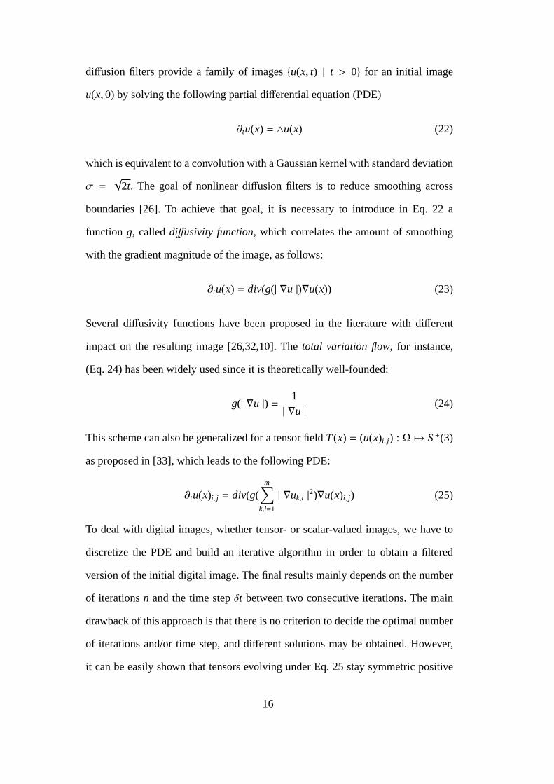
diffusion filters provide a family of imagesu(x, t) | t > 0 for an initial image

u(x,0) by solving the following partial differential equation (PDE)

∂tu(x) = 4u(x) (22)

which is equivalent to a convolution with a Gaussian kernel with standard deviation

σ =√

2t. The goal of nonlinear diffusion filters is to reduce smoothing across

boundaries [26]. To achieve that goal, it is necessary to introduce in Eq. 22 a

function g, calleddiffusivity function, which correlates the amount of smoothing

with the gradient magnitude of the image, as follows:

∂tu(x) = div(g(| ∇u |)∇u(x)) (23)

Several diffusivity functions have been proposed in the literature with different

impact on the resulting image [26,32,10]. Thetotal variation flow, for instance,

(Eq. 24) has been widely used since it is theoretically well-founded:

g(| ∇u |) =1| ∇u |

(24)

This scheme can also be generalized for a tensor fieldT(x) = (u(x)i, j) : Ω 7→ S+(3)

as proposed in [33], which leads to the following PDE:

∂tu(x)i, j = div(g(m∑

k,l=1

| ∇uk,l |2)∇u(x)i, j) (25)

To deal with digital images, whether tensor- or scalar-valued images, we have to

discretize the PDE and build an iterative algorithm in order to obtain a filtered

version of the initial digital image. The final results mainly depends on the number

of iterationsn and the time stepδt between two consecutive iterations. The main

drawback of this approach is that there is no criterion to decide the optimal number

of iterations and/or time step, and different solutions may be obtained. However,

it can be easily shown that tensors evolving under Eq. 25 stay symmetric positive

16

definite if the initial valueT(0) = (u(0)i, j) is symmetric positive definite [6].

5 Results

In this section, we present various numerical experiments and compare the

regularization methods previously detailed on synthetic and real DT-MRI data.

5.1 Synthetic Data

Experiment 1

In order to check the performance of our approach we generate a 50× 50 × 50

synthetic field of 3× 3 tensors which roughly simulates a bifurcation of two fibers.

In Fig. 4, we display a partial view of one slice in our volume, without noise

on the left and with a low level of noise on the right. For this image, as well

as any other tensor field presented in this paper, the color code is related to the

fractional anisotropy (FA) of the tensors with: Blue= low FA / Red= high FA. To

generate the noise we use a generalization of the Gaussian distribution for samples

belonging toS+(3). By using the algorithm proposed in [19], we can easily generate

a set of random positive definite tensors with the desired mean and covariance

matrix. This is a much more satisfying approach than, as usually done, simply

building symmetric matrices with iid normally distributed components and then

enforcing their positiveness since this leaves no grasp on the actual distribution

of the tensors. Moreover, the algorithm proposed in [19] is consistent with the

parametric model for noise in DT-MRI proposed in [23]. In this work, the authors

proved that, assuming that the magnitude diffusion weighted images are Rician

distributed, noise in diffusion tensor data within a voxel follows a 6-dimensional

17

Fig. 4. Left: Original synthetic dataset. Right: Noisy image./ Color code: Blue= low FA

and Red= high FA

Normal distribution. We then try to recover the original image from the noisy

version. Figures 5 compares the outputs of the filtering schemes presented in this

paper from a qualitative point of view. The image on the left was obtained by

convolving each component of the tensor with a Gaussian kernel (σ = 1.5). This

is equivalent to the diffusion process presented in Eq. 22. In the middle we can

see the best output we have obtained with the nonlinear diffusion process presented

in Eq. 25 with time step 0.01 and 36 iterations. The result on the right uses our

anisotropic Riemannian approach presented in section 4.1. We must point out here

that the optimization of the diffusion time for the nonlinear diffusion scheme is

clearly both critical and difficult to adjust. It is definitely a major limitation of this

last approach. From Fig. 5, it is obvious that boundaries are better preserved by

anisotropic methods than by the isotropic approach. To more clearly emphasize

these different behaviors, Fig. 6 shows a detail of the output of the Gaussian

filtering scheme and of the anisotropic Riemannian approach. In order to quantify

and compare the performances of the nonlinear diffusion with our Riemannian

anisotropic smoothing method, we propose to measure the error at each voxel by

18

Fig. 5. Results on denoising synthetic data. Left: Gaussian convolution (Eq. 22). Middle:

Nonlinear diffusion (Eq. 25). Right: Anisotropic Riemannian filtering (section 4.1).

Fig. 6. Detail of boundaries. Left: Gaussian filtering (Eq. 22). Right: Anisotropic

Riemannian filtering (section 4.1).

using the squared geodesic distance between tensors:

Error(x) = D2(Σ(x), Σ(x)) (26)

whereΣ(x) is the original tensor field andΣ(x) is the filtered one. Table 1 shows

some statistics on the error, where it can be seen that the Riemannian approach

improves the behavior of the Euclidean counterparts. Since using the geodesic error

metric may bias the comparison in favor of our approach, another error measure is

also used in table 2. It shows the statistics of the Frobenius norm of the difference

19

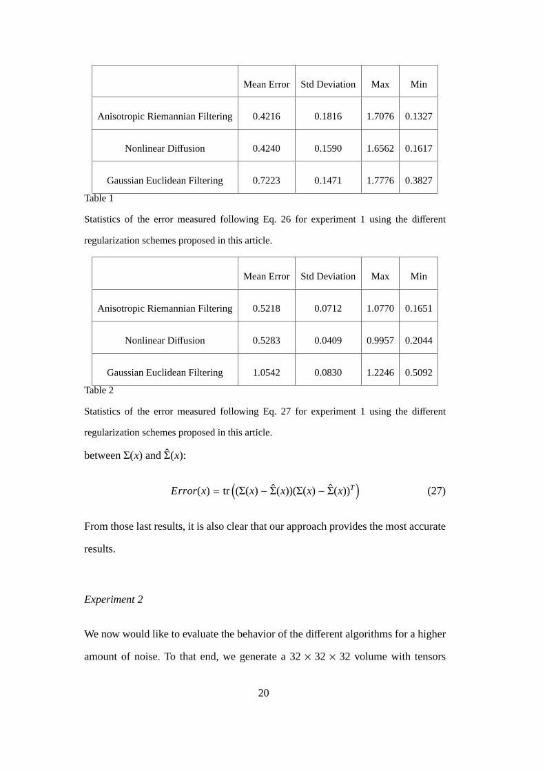
Mean Error Std Deviation Max Min

Anisotropic Riemannian Filtering 0.4216 0.1816 1.7076 0.1327

Nonlinear Diffusion 0.4240 0.1590 1.6562 0.1617

Gaussian Euclidean Filtering 0.7223 0.1471 1.7776 0.3827

Table 1

Statistics of the error measured following Eq. 26 for experiment 1 using the different

regularization schemes proposed in this article.

Mean Error Std Deviation Max Min

Anisotropic Riemannian Filtering 0.5218 0.0712 1.0770 0.1651

Nonlinear Diffusion 0.5283 0.0409 0.9957 0.2044

Gaussian Euclidean Filtering 1.0542 0.0830 1.2246 0.5092

Table 2

Statistics of the error measured following Eq. 27 for experiment 1 using the different

regularization schemes proposed in this article.

betweenΣ(x) andΣ(x):

Error(x) = tr((Σ(x) − Σ(x))(Σ(x) − Σ(x))T

)(27)

From those last results, it is also clear that our approach provides the most accurate

results.

Experiment 2

We now would like to evaluate the behavior of the different algorithms for a higher

amount of noise. To that end, we generate a 32× 32 × 32 volume with tensors

20

oriented along the vertical direction and introduce a 16× 16× 16 cube with tensors

oriented in the orthogonal direction, as shown in the top left image of Fig. 7. Then,

we add a high level of Gaussian noise, resulting in the noisy tensor field in the

top right image of Fig. 7. The bottom right image corresponds to the anisotropic

Riemannian filtering approach proposed in this paper while the image on the left

is the output of the nonlinear diffusion. Differences arise when comparing these

two images. First of all, noise is better removed with the Riemannian approach

than with the nonlinear diffusion, where some misoriented tensors remain even

after 536 iterations with a time step of 0.01, which are the parameters that provide

the optimal response. Furthermore, the well-known swelling effect, due to a faster

regularization of the eigenvalues, is observed for the nonlinear diffusion, whereas

it is not noticeable for our Riemannian approach. This can be observed by looking

at the colors of the tensors: First, we point out that the original tensors are blue

because they are all identical, thus have the same FA (0.77), and our visualization

software assigns the color associated to the lowest value in that case. But most

importantly, we can see that the regularized tensor field obtained with our approach

is more anisotropic (tensors are yellow and FA is around 0.75) than that obtained

with the nonlinear diffusion (tensors are green and FA is around 0.60). From a

quantitative point of view, we measure the error between the original and the

regularized images following Eq. 26 and Eq, 27. As shown in table 3, mean squared

geodesic distance is much lower for the anisotropic Riemannian approach than for

the nonlinear diffusion. Table 4 shows the error statistics based on the Frobenius

norm. It is also obvious that the accuracy of the Riemannian approach is much

better than that achieved with the nonlinear diffusion.

21

Fig. 7. Results in presence of a high level of noise. Top Left: Original Image. Top

Right: Noisy Image. Bottom Left: Nonlinear diffusion (Eq. 25). Bottom Right: Anisotropic

Riemannian filtering (section 4.1).

Mean Error Std. Deviation Max Min

Anisotropic Riemannian Filtering 0.2572 0.1313 1.3065 0.0300

Nonlinear Diffusion 0.8284 0.1209 3.2551 0.2630

Table 3

Statistics of the error measured following Eq. 26 for experiment 2.

22

Mean Error Std. Deviation Max Min

Anisotropic Riemannian Filtering 0.6296 0.5166 4.4222 0.0600

Nonlinear Diffusion 2.1677 0.7970 91.2742 0.7367

Table 4

Statistics of the error measured following Eq. 27 for experiment 2.

5.2 Real DT-MRI Data

For experiments with real data, diffusion weighted images were acquired on a

3 Tesla MEDSPEC 30/80 AVANCE (Bruker) at the Centre IRMf de Marseille,

France, using a quadrature bird-cage head coil. We used 12 gradient directions and

a b-value of 1000 s/mm2. Acquisitions were repeated 8 times for each direction

to ensure a good signal-to-noise ratio. The sequence parameters were chosen as

follows: ∆ = 38.5ms,δ = 21.6ms,TR = 10000ms,T E = 79ms and voxel size

was 2× 2× 2 mm3. Diffusion tensors were estimated by a robust gradient descent

algorithm preserving their symmetry and positive definiteness, as presented in [19].

The idea of this method is to minimize a functional of the linearized Stejskal-Tanner

equation by evolving an initial guess of the tensor on the manifoldS+(3) with a

numerical scheme similar to the one used for the estimation of the mean. Figure

8 (top left) shows the estimated diffusion tensors. On the top right, we display the

regularized image using the Riemannian filtering approach, while bottom images

are regularized using nonlinear diffusion, both with 10 iterations, but different

time steps: 0.001 on the left and 0.01 on the right. If we analyze the different

structures found on this axial slice, we can see that tensors orientation within the

splenium of the corpus callosum(CC(S) in the image) and in thegenu of the corpus

callosum(CC(G) in the image) is more coherent with our Riemannian filtering

23

Fig. 8. Results on real DT-MRI data. Top Left: Original DT-MRI data. CC(S): Splenium of

the Corpus Callosum. CC(G): Genu of the Corpus Callosum. VE: Ventricles. CR: Corona

Radiata. Top Right: anisotropic Riemannian filtering. Bottom Left: nonlinear diffusion

(time step 0.001, 10 iter.). Bottom Right: nonlinear diffusion (time step 0.01, 10 iter.)

scheme. Anisotropy in these areas is also better preserved than with the nonlinear

diffusion case, which yields blurred areas most likely because of the properties of

the Euclidean gradient. In addition, theventriclesareas (VE in the image), since

they are mainly homogeneous structures, are better regularized with our approach,

as inhomogeneities do not disappear with nonlinear diffusion. Finally, thecorona

radiata (CR in the image) is well preserved in our approach while it is completely

24

Fig. 9. Real data volume of a human brain.

Fig. 10. Raw tensor field (left) compared to regularized tensor field (right)

smoothed away from the image with longer diffusion time. On Fig. 9 we show a

complete human brain volume where fiber orientation is color coded as follows:

25

Red: Right-Left/ Green: Anterior-Posterior/ Blue: Inferior-Superior. Original data

is shown at the top of the image, while the filtered version is shown at the bottom.

An axial slice from that volume is presented on Fig. 10, where we compare original

data (on the left) with the filtered version (on the right) using our approach. It is

clear tensors belonging to particular fiber bundles have are more coherent while the

interfaces between the various tracts have been preserved.

6 Conclusions

We have presented a novel differential geometrical approach for the anisotropic

regularization of tensor fields, seen as fields of multivariate normal distributions.

We focused on the properties of the space of multivariate normal distributions

to introduce an affine invariant Riemannian metric and notions such as the mean

and spatial gradient which provide a well-founded framework to develop a non

iterative anisotropic filtering algorithm for tensor data. The anisotropic behavior is

introduced through the gradient magnitude, simply computed by using the geodesic

distance between distributions. This gradient magnitude, contrary to the Euclidean

one, benefits from the affine invariance of the underlying distance. It is not sensitive

to the scale of the tensors which allows to better discriminate tissues interfaces

and regularize misoriented tensors because of the noise as shown in our numerical

experiments. Our filtering scheme is also compared to nonlinear diffusion of

matrix-valued data to point out its added value over the PDE-based approaches

and to show that our approach can easily solve some of their limitations, yielding

better results on synthetic and real DT-MRI data.

26

Acknowledgments

This research was partially supported by the European Commission (contract

FP6-507609), the French National Project ACI Obs-Cerv, the European Project

IMAVIS (HPMT-CT-2000-00040) and the Region Provence-Alpes-Cote d’Azur.

The authors would like to thank J.L. Anton, M. Roth and N. Wotawa for the human

brain DTI datasets used in this paper.

References

[1] S. Amari, Differential geometrical methods in statistics, Lectures Notes in Statistics,

Springer-Verlag (1990).

[2] C. Atkinson, A. Mitchell, Rao’s distance measure, Sankhya: The Indian Journal of

Stats. 43 (A) (1981) 345–365.

[3] P. Basser, J. Mattiello, D. LeBihan, MR diffusion tensor spectroscopy and imaging,

Biophysica (66) (1994) 259–267.

[4] J. Bigun, G.-H. Granlund, Optimal orientation detection of linear symmetry,

Proceedings of IEEE International Conference on Computer Vision, London (1987)

433–438.

[5] E. Boring, A. Pang, Interactive deformations from tensor fields, Proceedings of IEEE

Visualization (1998) 297–304.

[6] T. Brox, J. Weickert, B. Burgeth, P. Mrazek, Nonlinear structure tensors, Image and

Vision Computing, 24 (1), (January 2006) 41-55.

[7] J. Burbea, C. Rao, Entropy differential metric, distance and divergence measures in

probability spaces: A unified approach, Journal of Multivariate Analysis 12 (1982)

575–596.

27

[8] J. Burbea, Informative geometry of probability spaces, Expositiones Mathematica

43 (A) (1986) 345–365.

[9] M. Calvo, J. Oller, An explicit solution of information geodesic equations for the

multivariate normal model, Statistics and Decisions 9 (1991) 119–138.

[10] P. Charbonnier, G. Aubert, M. Blanc-Fraud, M. Barlaud, Two deterministic half-

quadratic regularization algorithms for computed imaging, Proceedings of the

International Conference on Image Processing Vol.2 (1994) 168–172.

[11] C. Chefd’hotel, D. Tschumperle, R. Deriche, O. Faugeras, Constrained flows on

matrix-valued functions : Application to diffusion tensor regularization, Proceedings

of the European Conference on Computer Vision, Copenhaguen (2002), 251–265.

[12] O. Coulon, D. Alexander, S. Arridge, Diffusion tensor magnetic resonance image

regularisation, Medical Image Analysis 8 (1) (2004) 47–67.

[13] P. Eriksen, Geodesics connected with the fisher metric on the multivariate manifold,

Tech. Rep. 86-13, Institute of Electronic Systems, Aalborg University (1986).

[14] P. Fletcher, S. Joshi, Principal geodesic analysis on symmetric spaces: Statistics of

diffusion tensors, Proceedings of Computer Vision Approaches to Medical Image

Analysis, Prague (2004) 87–98.

[15] W. Forstner, B. Moonen, A metric for covariance matrices, Tech. rep., Stuttgart

University, Dept. of Geodesy and Geoinformatics (1999).

[16] H. Karcher, Riemannian centre of mass and mollifier smoothing, Comm. Pure Appl.

Math 30 (1977) 509–541.

[17] C. Lenglet, M. Rousson, R. Deriche, O. Faugeras, Statistics on multivariate normal

distributions: A geometric approach and its application to Diffusion Tensor MRI,

INRIA Research Report 5242 (June 2004).

28

[18] C. Lenglet, M. Rousson, R. Deriche, O. Faugeras, Statistics on the manifold of

multivariate normal distributions: Theory and application to Diffusion Tensor MRI,

Journal of Mathematical Imaging and Vision, Special Issue MIA’04 (2006) In press.

[19] C. Lenglet, R. Deriche, O. Faugeras, S. Lehericy, K. Ugurbil, A Riemannian approach

to diffusion tensors estimation and streamline-based fiber tracking, Proceedings of

11th Annual Meeting of the Organization for Human Brain Mapping, Toronto (2005).

[20] M. Lovric, M. Min-Oo, E.-A. Ruh, Multivariate normal distributions parametrized as

a Riemannian symmetric space, J. Multivariate Analysis 74 (1) (2005) 36–48.

[21] C.-A. Micchelli, L. Noakes, Rao distances, J. Multivariate Analysis 92 (2005) 97–115.

[22] M. Moakher, A differential geometric approach to the geometric mean of symmetric

positive-definite matrices, SIAM J. Matrix Anal. Appl. 26 (3) (2005) 735–747.

[23] S. Pajevic, P. Basser, Parametric and non-parametric statistical analysis of DT-MRI

data, Journal of Magnetic Resonance (161) (2003) 1–14.

[24] X. Pennec, Probabilities and statistics on Riemannian manifolds: A geometric

approach, INRIA Research Report 5093 (January 2004).

[25] X. Pennec, P. Fillard, N. Ayache, A Riemannian framework for tensor computing,

International Journal of Computer Vision 66 (1) (2006) 41–66.

[26] P. Perona, J. Malik, Scale-space and edge detection using anisotropic diffusion, IEEE

Transactions on Pattern Analysis and Machine Intelligence 12 (7) (1990) 629–639.

[27] C. Rao, Information and accuracy attainable in the estimation of statistical parameters,

Bull. Calcutta Math. Soc. 37 (1945) 81–91.

[28] L. Skovgaard, A Riemannian geometry of the multivariate normal model, Tech. Rep.

81/3, Statistical Research Unit, Danish Medical Research Council, Danish Social

Science Research Council (1981).

29

[29] D. Tschumperle, R. Deriche, Variational frameworks for DT-MRI estimation,

regularization and visualization, Proceedings of the International Conference on

Computer Vision, Nice (2003), 116–122.

[30] D. Tschumperle, R. Deriche, DT-MRI images : Estimation, regularization and

application, Proceedings of the International Workshop on Computer Aided Systems

Theory, Las Palmas de Gran Canaria (2003), 530–541.

[31] Z. Wang, B. Vemuri, Y. Chen, T. Mareci, A constrained variational principle for direct

estimation and smoothing of the diffusion tensor field from complex DWI, IEEE

Transactions on Medical Imaging 23 (8) (2004) 930–939.

[32] J. Weickert, Anisotropic Diffusion in Image Processing, Teubner-Verlag (1998).

[33] J. Weickert, T. Brox, Diffusion and regularization of vector- and matrix-valued images,

Inverse Problems, Image Analysis and Medical Imaging. Contemporary Mathematics

313 (2002) 251–268.

[34] C.-F. Westin, S. Maier, H. Mamata, A. Nabavi, F.-A. Jolesz, R. Kikinis, Processing and

visualization for Diffusion Tensor MRI, Medical Image Analysis 6 (2) (2002) 93–108.

[35] E.-A. Witalis, Incompressible steady flow with tensor conductivity leaving a transverse

magnetic field, J. Nucl. Energy, Part C Plasma Phys. 8 (1966) 137–143.

30