Enhancement of Flow-Like Structures in Hyperspectral Imagery using Tensor Nonlinear Anisotropic Diffusion

Maider Marin-McGee and Miguel Velez-Reyes Laboratory for Applied Remote Sensing and Image Processing

University of Puerto Rico at Mayaguez E-mail: Maider.Marin, Miguel.Velez-Reyes@upr.edu

ABSTRACT

Analyzing flow-like patterns in images for image understanding is an active research area but there have been much less attention paid to the process of enhancement of those structures. The completion of interrupted lines or the enhancement of flow-like structures is known as Coherence-Enhancement (CE). In this work, we are studying nonlinear anisotropic diffusion filtering for coherence enhancement. Anisotropic diffusion is commonly used for edge enhancement by inhibiting diffusion in the direction of highest spatial fluctuation. For CE, diffusion is promoted along the direction of lowest spatial fluctuation in a neighborhood thereby taking into account how strongly the local gradient of the structures in the image is biased towards that direction. Results of CE applied multispectral and hyperspectral images are presented. Keywords: Hyperspectral Image Processing, Nonlinear Diffusion, Coherence-Enhancement, Image Processing.

1 INTRODUCTION The most stable and reliable descriptor of the local structure of an image is the structure tensor [1]. This tensor is a symmetric

positive semi definite matrix that at each pixel determines the orientation of minimum and maximum spatial fluctuation in a neighborhood of a pixel. It was presented by [2] and also by [3] in an equivalent formulation for gray level imagery. The structure tensor is derived from the gradient; it provides the main directions of the gradient in a specified neighborhood of a point. Its eigen-decomposition provides information of how strongly the gradient is biased towards a particular direction which is known as coherence [4]. Oriented flow-like structures can be found by looking to the orientation of lowest spatial fluctuation in an image, and it is determined by the eigenvector of the structure tensor with the smallest eigenvalue. This process has been studied in the context of gray and color images [5] by the pattern recognition and computer vision fields and used for automatic grading of fabrics or wood surfaces [6], segmenting two-photon laser scanning microscopy images[7], enhancing fingerprint images [1], enhancing corners [2] and 3-D medical imaging [3,6]. But few have been done with vector-valued data such as multispectral (MSI) and hyperspectral images (HSI).

This paper study a PDE-based coherence diffusion method proposed by [6] and uses a finite volume scheme proposed by [7]. The main contribution in this paper is to extend CED to MSI and HSI, and propose eigenvalues for the diffusion tensor. In addition, it will be shown that coherence enhancement can be used for remote sensing image processing problems. Results will be presented for multispectral, and hyperspectral images. This paper is organized as follows. Section 2 introduces CED, the diffusion tensor, and some properties. Section 3 presents an overview of finite volume discretization. Section 4 shows some experimental results.

2 COHERENCE ENHANCING DIFFUSION Adaptive smoothing methods are based on the idea of applying a process which itself depends on local properties of the image. A

regularized adaptive method can be extended to anisotropic processes which make use of an adapted diffusion tensor instead of scalar diffusivity. This is the case of the anisotropic diffusion model introduced by Weickert in [1,6]. Let us consider a scale image domain

1 2: (0, ) (0, )n nΩ = × with 1n number of rows and 2n number of columns, boundary ∂Ω and : (0, )I = ∞ . The following initial boundary value problem represents a class of anisotropic diffusion filters:

( ) 0 inu D u It

∂−∇⋅ ∇ = Ω×

∂ (1.1)

( ) ( ),0 in u x f x= Ω (1.2)

Algorithms and Technologies for Multispectral, Hyperspectral, and Ultraspectral Imagery XVII,edited by Sylvia S. Shen, Paul E. Lewis, Proc. of SPIE Vol. 8048, 80480E · © 2011 SPIE

CCC code: 0277-786X/11/$18 · doi: 10.1117/12.885645

Proc. of SPIE Vol. 8048 80480E-1

Downloaded from SPIE Digital Library on 08 Sep 2011 to 136.145.56.95. Terms of Use: http://spiedl.org/terms

, 0 onD u n I∇ = ∂Ω× (1.3)

Hereby, u, the filtered version of image f (x), is the solution of the initial boundary value problem for the diffusion equation with f as initial condition, see Equation (1.2). Equation (1.1) has a partial derivative with respect to time, in image processing there is no real evolution in time, variable t in this case is a dummy variable that represent an iterative process. The vector n denotes the outer normal unit vector to ∂Ω and ⟨· , ·⟩ is the Euclidean scalar product on ℜ2 Equation (1.3) is a Neumann boundary condition, which means that the flux is zero outside the boundary. Equations (1.1) to (1.3) will be called P1. CED is basically a 1-D diffusion, where a minimal amount of isotropic smoothing is added for regularization purposes.

In order to make the diffusion tensor 22×ℜ∈D adaptive, in the sense that a strong smoothing is obtained in one direction and low smoothing along the edges, it will depend on the structure tensor that in turn depends on the edge estimator uσ∇ , which is also

known as the smoothed gradient. uσ∇ is obtained by finding the gradient of the smoothed image uσ obtained by a Gaussian

convolution Gσ of variance 0σ >

( ) ( ) ( ), : , , 0u x t G u t xσ σ σ= ∗ ⋅ >% (1.4)

( )2

221: exp ,

22

xGσ σπσ

⎛ ⎞⎜ ⎟= ⋅ −⎜ ⎟⎝ ⎠

(1.5)

where u% denotes the extension of u from Ω to ℜ2×2 that can be obtained by mirroring at ∂Ω [8] and the * is a convolution.

Figure 1 shows a block diagram of CED for a scalar image. The following sections will discuss some of these steps.

Figure 1. CED block diagram showing an iteration for scale t = n and for a scalar image.

2.1 Diffusion Tensor The diffusion tensor D was designed to generate a strong smoothing in a preferred direction and a low smoothing perpendicular to it, e.g. for images with interrupted coherence of structures, D is built upon the structure tensor Jρ . This tensor provides the main directions of the gradient in a specified neighborhood of a point. Its eigen-decomposition

Proc. of SPIE Vol. 8048 80480E-2

Downloaded from SPIE Digital Library on 08 Sep 2011 to 136.145.56.95. Terms of Use: http://spiedl.org/terms

S

provides information of how strongly the gradient is biased towards a particular direction, which is known as coherence direction. For the oriented flow-like case, we want the direction of lowest spatial fluctuation in the image. The structure tensor is defined by [6]:

0J G Jρ ρ= ∗

where 0 ,TJ u uσ σ= ∇ ∇ with , 0σ ρ > , u and Gσ are as in Equations (1.4) and (1.5). 0J is a 2 2× symmetric, positive semi-definite matrix and its eigenvectors are parallel and orthogonal to uσ∇ . Why choose the structure tensor as an outer product and do not use directly the smoothed gradient? Cottet et al [9] presented a reaction-diffusion model where the diffusion was along the eigenvector corresponding to the smallest eigenvalue, ( )2

2 g uσκ = ∇ of its diffusion tensor,

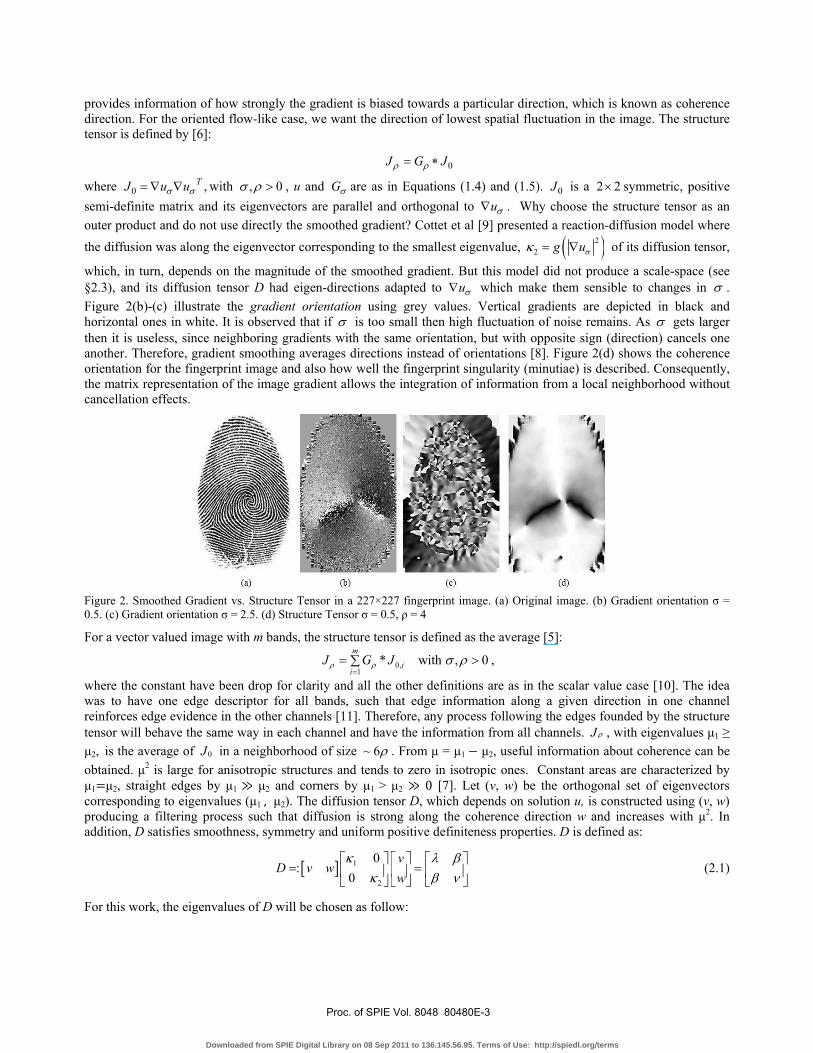
which, in turn, depends on the magnitude of the smoothed gradient. But this model did not produce a scale-space (see §2.3), and its diffusion tensor D had eigen-directions adapted to uσ∇ which make them sensible to changes in σ . Figure 2(b)-(c) illustrate the gradient orientation using grey values. Vertical gradients are depicted in black and horizontal ones in white. It is observed that if σ is too small then high fluctuation of noise remains. As σ gets larger then it is useless, since neighboring gradients with the same orientation, but with opposite sign (direction) cancels one another. Therefore, gradient smoothing averages directions instead of orientations [8]. Figure 2(d) shows the coherence orientation for the fingerprint image and also how well the fingerprint singularity (minutiae) is described. Consequently, the matrix representation of the image gradient allows the integration of information from a local neighborhood without cancellation effects.

Figure 2. Smoothed Gradient vs. Structure Tensor in a 227×227 fingerprint image. (a) Original image. (b) Gradient orientation σ = 0.5. (c) Gradient orientation σ = 2.5. (d) Structure Tensor σ = 0.5, ρ = 4

For a vector valued image with m bands, the structure tensor is defined as the average [5]:

0,1

* with , 0m

ii

J G Jρ ρ σ ρ=

= >∑ ,

where the constant have been drop for clarity and all the other definitions are as in the scalar value case [10]. The idea was to have one edge descriptor for all bands, such that edge information along a given direction in one channel reinforces edge evidence in the other channels [11]. Therefore, any process following the edges founded by the structure tensor will behave the same way in each channel and have the information from all channels. J ρ , with eigenvalues μ1 ≥ μ2, is the average of 0J in a neighborhood of size ~ 6ρ . From μ = μ1 − μ2, useful information about coherence can be obtained. μ2 is large for anisotropic structures and tends to zero in isotropic ones. Constant areas are characterized by μ1=μ2, straight edges by μ1 ≫ μ2 and corners by μ1 > μ2 ≫ 0 [7]. Let (v, w) be the orthogonal set of eigenvectors corresponding to eigenvalues (μ1 , μ2). The diffusion tensor D, which depends on solution u, is constructed using (v, w) producing a filtering process such that diffusion is strong along the coherence direction w and increases with μ2. In addition, D satisfies smoothness, symmetry and uniform positive definiteness properties. D is defined as:

[ ] 1

2

0:

0v

D v ww

κ λ βκ β ν

⎡ ⎤ ⎡ ⎤ ⎡ ⎤= =⎢ ⎥ ⎢ ⎥ ⎢ ⎥

⎣ ⎦ ⎣ ⎦⎣ ⎦ (2.1)

For this work, the eigenvalues of D will be chosen as follow:

Proc. of SPIE Vol. 8048 80480E-3

Downloaded from SPIE Digital Library on 08 Sep 2011 to 136.145.56.95. Terms of Use: http://spiedl.org/terms

10 1 <<<= αακ

1 2

2 41 2

(1 )exp elseC

α μ μ

κ α αμ μψ

=⎧ ⎛ ⎞⎪ ⎜ ⎟⎪= ⎜ ⎟⎨ + − −⎜ ⎟⎪ −⎛ ⎞⎜ ⎟⎪ ⎜ ⎟

⎝ ⎠⎩ ⎝ ⎠

(2.2)

Note that by definition ( )2 0,1 ,κ α∈ is a small number that guarantees that the process never stops and keeps the

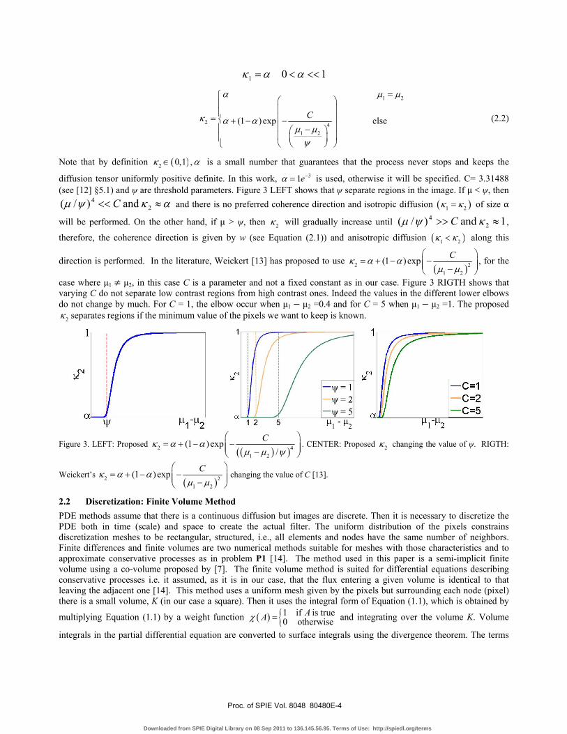
diffusion tensor uniformly positive definite. In this work, 31eα −= is used, otherwise it will be specified. C= 3.31488 (see [12] §5.1) and ψ are threshold parameters. Figure 3 LEFT shows that ψ separate regions in the image. If μ < ψ, then

ακψμ ≈<< 24 and )/( C and there is no preferred coherence direction and isotropic diffusion ( )1 2κ κ= of size α

will be performed. On the other hand, if μ > ψ, then 2κ will gradually increase until 1 and )/( 24 ≈>> κψμ C ,

therefore, the coherence direction is given by w (see Equation (2.1)) and anisotropic diffusion ( )1 2κ κ< along this

direction is performed. In the literature, Weickert [13] has proposed to use ( )2 2

1 2

(1 )exp Cκ α αμ μ

⎛ ⎞= + − −⎜ ⎟⎜ ⎟−⎝ ⎠

, for the

case where μ1 ≠ μ2, in this case C is a parameter and not a fixed constant as in our case. Figure 3 RIGTH shows that varying C do not separate low contrast regions from high contrast ones. Indeed the values in the different lower elbows do not change by much. For C = 1, the elbow occur when μ1 − μ2 =0.4 and for C = 5 when μ1 − μ2 =1. The proposed

2κ separates regions if the minimum value of the pixels we want to keep is known.

Figure 3. LEFT: Proposed ( )( )2 4

1 2

(1 )exp/

Cκ α αμ μ ψ

⎛ ⎞= + − −⎜ ⎟⎜ ⎟−⎝ ⎠

. CENTER: Proposed 2κ changing the value of ψ. RIGTH:

Weickert’s ( )2 2

1 2

(1 )exp Cκ α αμ μ

⎛ ⎞= + − −⎜ ⎟⎜ ⎟−⎝ ⎠

changing the value of C [13].

2.2 Discretization: Finite Volume Method PDE methods assume that there is a continuous diffusion but images are discrete. Then it is necessary to discretize the PDE both in time (scale) and space to create the actual filter. The uniform distribution of the pixels constrains discretization meshes to be rectangular, structured, i.e., all elements and nodes have the same number of neighbors. Finite differences and finite volumes are two numerical methods suitable for meshes with those characteristics and to approximate conservative processes as in problem P1 [14]. The method used in this paper is a semi-implicit finite volume using a co-volume proposed by [7]. The finite volume method is suited for differential equations describing conservative processes i.e. it assumed, as it is in our case, that the flux entering a given volume is identical to that leaving the adjacent one [14]. This method uses a uniform mesh given by the pixels but surrounding each node (pixel) there is a small volume, K (in our case a square). Then it uses the integral form of Equation (1.1), which is obtained by

multiplying Equation (1.1) by a weight function ( ) 1 if is true0 otherwise

AAχ = and integrating over the volume K. Volume

integrals in the partial differential equation are converted to surface integrals using the divergence theorem. The terms

Proc. of SPIE Vol. 8048 80480E-4

Downloaded from SPIE Digital Library on 08 Sep 2011 to 136.145.56.95. Terms of Use: http://spiedl.org/terms

t=80 t= 100

t=30

t= 150

t= 50

t=200

Original Image p=1- p=4

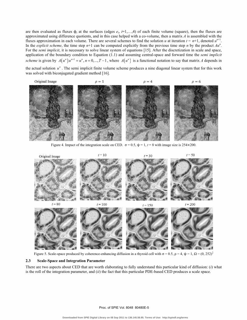
are then evaluated as fluxes ϕi at the surfaces (edges ei, i=1,…,4) of each finite volume (square), then the fluxes are approximated using difference quotients, and in this case helped with a co-volume, then a matrix A is assembled with the fluxes approximation in each volume. There are several schemes to find the solution u at iteration t = n+1, denoted un+1. In the explicit scheme, the time step n+1 can be computed explicitly from the previous time step n by the product Aun. For the semi implicit, it is necessary to solve linear system of equations [15]. After the discretization in scale and space, application of the boundary condition to Equation (1.1) and assuming central-space and forward time the semi implicit scheme is given by ( ) 1 , 0,..., 1n n nA u u u n T+ = = − , where ( )nA u is a functional notation to say that matrix A depends in

the actual solution nu . The semi implicit finite volume scheme produces a nine diagonal linear system that for this work was solved with biconjugated gradient method [16].

Figure 4. Impact of the integration scale on CED. σ = 0.5, ψ = 1, t = 8 with image size is 254×200.

Figure 5. Scale-space produced by coherence-enhancing diffusion in a thyroid cell with σ = 0.5, ρ = 4, ψ = 1, Ω = (0, 252)2

2.3 Scale-Space and Integration Parameter There are two aspects about CED that are worth elaborating to fully understand this particular kind of diffusion: (i) what is the roll of the integration parameter, and (ii) the fact that this particular PDE-based CED produces a scale space.

Proc. of SPIE Vol. 8048 80480E-5

Downloaded from SPIE Digital Library on 08 Sep 2011 to 136.145.56.95. Terms of Use: http://spiedl.org/terms

2.3.1 Integration Parameter Recall from Section 2.1 that the structure tensor J ρ is the average of the gradient orientations in a neighborhood of size ρ. Figure 4 shows an example of how the size of ρ influence the result of CED. In this figure, the Van Gogh paint [17] is shown, all parameters are kept constant except the integration parameter. When ρ = 1, the filter will produce artifacts, while increasing it to ρ = 4 make flow-like structures look like completed lines since the average of orientations in this bigger neighborhood captures the coherence orientation, but further increase to ρ = 6 hardly makes any difference [12]

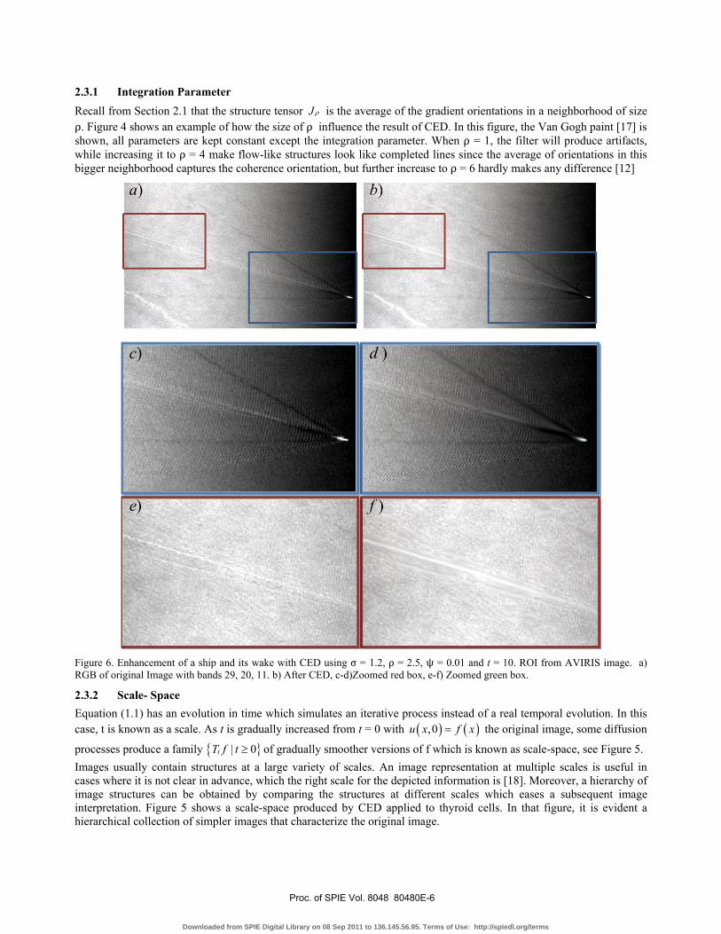
Figure 6. Enhancement of a ship and its wake with CED using σ = 1.2, ρ = 2.5, ψ = 0.01 and t = 10. ROI from AVIRIS image. a) RGB of original Image with bands 29, 20, 11. b) After CED, c-d)Zoomed red box, e-f) Zoomed green box.

2.3.2 Scale- Space Equation (1.1) has an evolution in time which simulates an iterative process instead of a real temporal evolution. In this case, t is known as a scale. As t is gradually increased from t = 0 with ( ) ( ),0u x f x= the original image, some diffusion

processes produce a family | 0tT f t ≥ of gradually smoother versions of f which is known as scale-space, see Figure 5. Images usually contain structures at a large variety of scales. An image representation at multiple scales is useful in cases where it is not clear in advance, which the right scale for the depicted information is [18]. Moreover, a hierarchy of image structures can be obtained by comparing the structures at different scales which eases a subsequent image interpretation. Figure 5 shows a scale-space produced by CED applied to thyroid cells. In that figure, it is evident a hierarchical collection of simpler images that characterize the original image.

Proc. of SPIE Vol. 8048 80480E-6

Downloaded from SPIE Digital Library on 08 Sep 2011 to 136.145.56.95. Terms of Use: http://spiedl.org/terms

S

= 0.05 11) = 0.2

3 EXPERIMENTAL RESULTS Experiments on enhancement of HSI and multispectral remote sensed data are presented in this section. In addition a discussion of the components of the diffusion tensor is provided.

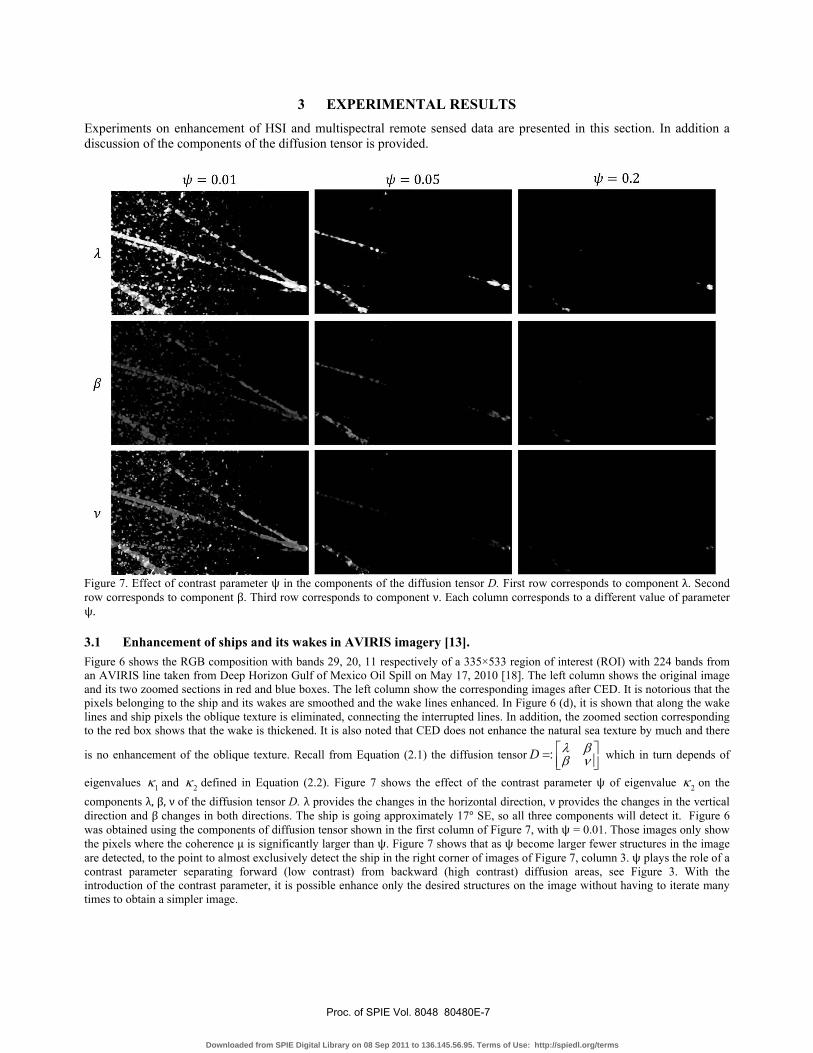
Figure 7. Effect of contrast parameter ψ in the components of the diffusion tensor D. First row corresponds to component λ. Second row corresponds to component β. Third row corresponds to component ν. Each column corresponds to a different value of parameter ψ. 3.1 Enhancement of ships and its wakes in AVIRIS imagery [13]. Figure 6 shows the RGB composition with bands 29, 20, 11 respectively of a 335×533 region of interest (ROI) with 224 bands from an AVIRIS line taken from Deep Horizon Gulf of Mexico Oil Spill on May 17, 2010 [18]. The left column shows the original image and its two zoomed sections in red and blue boxes. The left column show the corresponding images after CED. It is notorious that the pixels belonging to the ship and its wakes are smoothed and the wake lines enhanced. In Figure 6 (d), it is shown that along the wake lines and ship pixels the oblique texture is eliminated, connecting the interrupted lines. In addition, the zoomed section corresponding to the red box shows that the wake is thickened. It is also noted that CED does not enhance the natural sea texture by much and there

is no enhancement of the oblique texture. Recall from Equation (2.1) the diffusion tensor :D λ ββ ν⎡ ⎤= ⎢ ⎥⎣ ⎦

which in turn depends of

eigenvalues 1κ and 2κ defined in Equation (2.2). Figure 7 shows the effect of the contrast parameter ψ of eigenvalue 2κ on the components λ, β, ν of the diffusion tensor D. λ provides the changes in the horizontal direction, ν provides the changes in the vertical direction and β changes in both directions. The ship is going approximately 17° SE, so all three components will detect it. Figure 6 was obtained using the components of diffusion tensor shown in the first column of Figure 7, with ψ = 0.01. Those images only show the pixels where the coherence μ is significantly larger than ψ. Figure 7 shows that as ψ become larger fewer structures in the image are detected, to the point to almost exclusively detect the ship in the right corner of images of Figure 7, column 3. ψ plays the role of a contrast parameter separating forward (low contrast) from backward (high contrast) diffusion areas, see Figure 3. With the introduction of the contrast parameter, it is possible enhance only the desired structures on the image without having to iterate many times to obtain a simpler image.

Proc. of SPIE Vol. 8048 80480E-7

Downloaded from SPIE Digital Library on 08 Sep 2011 to 136.145.56.95. Terms of Use: http://spiedl.org/terms

Figure 8 shows a ROI of band 7 of an image acquired using MODIS sensor [20] taken from North America between Washington state and Alaska, with spatial resolution of 500 m [19]. Also highlighted in red and green boxes there are two regions of two different kinds of clouds with observable ship contamination plumes. The rightmost column shows the enhancement of the edges of the plumes using CED. It can be observed that the edges of the plumes are smoother; the sensor texture in the blue box is not enhanced as shown in blue box in Figure 9. The red box ROI is more difficult since it is desirable to enhance the plumes edges without disturbing the cloud textures which is significant. This goal is achieved by setting ψ small to capture the contrast between clouds and plumes and making σ = 4 so the process ignore the clouds as shown in red box in Figure 9.

Figure 8. ROI for Band 7 of MODIS image [19] with two smaller ROIs highlighted in red and green boxes. Blue Boxes: Plumes captured by altostratus clouds and its CED enhancement with σ = 1, ρ = 3, ψ = 1 and t = 10. Red Boxes: Plumes captured by altocumulus clouds and its CED with σ = 4, ρ = 6, ψ = 0.35 and t = 10.

Figure 9 Components λ, β, and ν of the diffusion tensor for the CED image of the red and blue boxes in Figure 8.

4 SUMMARY AND CONCUSIONS CED generates a scale-space evolution by means of a nonlinear anisotropic diffusion equation. Its diffusion tensor reflects the local image structure by using the same set of eigenvectors as the structure tensor. The latter is better suited to define the diffusion tensor than the smoothed gradient, since it does not produce cancellation effects and more information can be extracted from it. The eigenvalues of the diffusion tensor are chosen in such a way that diffusion acts mainly along the direction with the highest coherence, and becomes stronger when the coherence increases. The

Proc. of SPIE Vol. 8048 80480E-8

Downloaded from SPIE Digital Library on 08 Sep 2011 to 136.145.56.95. Terms of Use: http://spiedl.org/terms

proposed eigenvalue 2κ for the diffusion tensor D separates low contrast from high contrast diffusion areas; with this definition it is possible to customize the diffusion. It is easy to enhance desired structures since it is only necessary to know the minimum value of the pixel in the structure that will be enhanced. CED usefulness was illustrated by applying it to multispectral and hyperspectral images. In addition, this method can be used for remote sensing applications as the enhancement of ship wakes and contamination plumes in satellite data.

5 ACKNOWLEDGMENTS This material is based upon work supported by the U.S. Department of Homeland Security under Award Number 2008-ST-061- ED0001. The views and conclusions contained in this document are those of the authors and should not be interpreted as necessarily representing the official policies, either expressed or implied of U.S. Department of Homeland Security. The Authors thanks Isnardo Arenas and professors Paul Castillo and Olga Drblìková for useful comments during the implementation process and professor Badrinath Roysan from the University of Houston for providing the Thyroid Tissue image data set and the NASA Jet propulsion Laboratory for providing the AVIRIS image.

6 REFERENCES [1] J. Weickert, “Multiscale texture enhancement,” in Computer Analysis of Images and Patterns 970, V. Hlavàc and R. Šára,

Eds., pp. 230-237, Springer Berlin / Heidelberg (1995). [2] W. Fröstner and E. Gülch, “A Fast Operator for Detection and Precise Location of Distinct Points, Corners and Centers of

Circular Features,” in Proceedings of the ISPRS Intercommission Workshop on Fast Processing of Photogrammetric Data, pp. 281-305 (1987).

[3] J. Bigün and G. H. Granlund, “Optimal Orientation Detection of Linear Symmetry,” in IEEE First International Conference on Computer Vision, p. 433–438, London, Great Britain (1987).

[4] B. Jähne, Spatio-temporal image processing: theory and scientific applications, Springer (1993). [5] J. Weickert, “Coherence-enhancing diffusion of colour images,” Image Vision Comput. 17, 201-212 (1999). [6] J. Weickert, “Coherence-Enhancing Diffusion Filtering,” International Journal of Computer Vision 31, 111-127 (1999). [7] O. Drblíková and K. Mikula, “Convergence Analysis of Finite Volume Scheme for Nonlinear Tensor Anisotropic Diffusion

in Image Processing,” SIAM J. Numer. Anal. 46, 37–60 (2007) [doi:http://dx.doi.org/10.1137/070685038]. [8] F. Catte, P. L. Lions, J. M. Morel, and T. Coll, “Image selective smoothing and edge detection by nonlinear diffusion,” SIAM

J. Numer. Anal. 29, 182–193 (1992). [9] G. H. Cottet and L. Germain, “Image processing through reaction combined with nonlinear diffusion,” Mathematics of

Computation 61, 659–673 (1993). [10] J. Weickert, “Scale-Space Properties of Nonlinear Diffusion Filtering with a Diffusion Tensor,” Laboratory of

Technomathematics, University of Kaiserslautern, P.O (1994). [11] S. Di Zenzo, “A note on the gradient of a multi-image,” Computer Vision, Graphics, and Image Processing 33, 116 - 125

(1986) [doi:DOI: 10.1016/0734-189X(86)90223-9]. [12] J. Weickert, Anisotropic Diffusion in Image Processing, Teubner-Verlag (1998). [13] J. Weickert, “Coherence-Enhancing Diffusion Filtering,” International Journal of Computer Vision 31, 111-127 (1999). [14] J. Peiró and S. Sherwin, “Finite Difference, Finite Element and Finite Volume methods for partial differential equations,”

Handbook of Materials Modeling, 2415–2446 (2005). [15] J. C. Strikwerda, Finite difference schemes and partial differential equations, Society for Industrial Mathematics (2004). [16] Y. Saad, Iterative Methods for Sparse Linear Systems, Second Edition, 2nd ed., Society for Industrial and Applied

Mathematics (2003). [17] V. Van Gogh, Road with cypress and star (1890). [18] J. Weickert, B. M. T. H. Romeny, and M. A. Viergever, “Efficient and reliable schemes for nonlinear diffusion filtering,”

Image Processing, IEEE Transactions on 7, 398 -410 (1998) [doi:10.1109/83.661190]. [19] NASA, “Visible Composite,”

ftp://ladsweb.nascom.nasa.gov/allData/5/MOBRGB/2003/041/MOBRGB.A2003041.2025.005.2006343091024.jpg. [20] NASA, “About MODIS,” <http://modis.gsfc.nasa.gov/about/>.

Proc. of SPIE Vol. 8048 80480E-9

Downloaded from SPIE Digital Library on 08 Sep 2011 to 136.145.56.95. Terms of Use: http://spiedl.org/terms