Fresnel diffraction of substructured gratings

$: Fresnel diffraction of substructured gratings$
Optics Communications 249 (2005) 397–405

www.elsevier.com/locate/optcom

Fresnel similarity

Adolf W. Lohmann, Jorge Ojeda-Castaneda *

Lehrsthul fur Multimediakommunikation und Signalverarbeitung,Universitat Erlangen-Nurnberg Cauerstrabe 7,

D-91058 Erlangen, Germany

Department of Physics and Mathematics, School of Science, University of las Americas, Apartado Postal 100, Cholula 72820,

Puebla, Mexico

Received 2 August 2004; received in revised form 17 December 2004; accepted 26 January 2005

Abstract

We study Fresnel diffraction, in particular the similarity between an object, at plane z = 0, and its diffraction pattern,

at z > 0. We define a degree of similarity, r(z), which depends on the object and the distance z. Perfect self-imaging is

associated with a degree of similarity equal to unity, while imperfect self-imaging is classified by a degree between zero

and one. We derive the theory that allows us to find r(z), if the object is known. And we can synthesize an object that

exhibits a wanted r(z). We describe some novel applications.

� 2005 Published by Elsevier B.V.

Keywords: Fresnel diffraction; Self-imaging; Extended depth of field; Axial imaging; Optical correlations; Apodizers

1. Introduction

For several applications in optical instrumenta-

tion, such as Talbot and Lau interferometry [1,2],

array illuminators [3,4], photolithography [5,6],

and for compression and expansion of the depth

of field [7–13], it is relevant to compare an input

transmittance with its Fresnel diffraction pattern.

0030-4018/$ - see front matter � 2005 Published by Elsevier B.V.

doi:10.1016/j.optcom.2005.01.042

* Corresponding author. Tel.: +522222292045; fax:

+522222292066.

E-mail address: [email protected] (J. Ojeda-Castane-

da).

Here, we aim to analyze quantitatively the blur-

ring due to Fresnel diffraction. To that end, we for-mulate a Fresnel diffraction theory in a way that

tells us how to manipulate the diffraction blur.

Our theoretical tool is a modified cross correlation

between the input object u0(x), at plane z = 0, and

its Fresnel diffraction pattern u(x,z), at plane

z > 0. This cross correlation is denoted as the sim-

ilarity function.

In Section 2, we begin by describing the under-lying fundamentals, and by standardizing the basic

terms. We also study some basic properties and

symmetries. We show how the power spectrum

mailto:[email protected]

SOURCE

(a)

398 A.W. Lohmann, J. Ojeda-Castaneda / Optics Communications 249 (2005) 397–405

of the object influences the degree of similarity.

Next, in Section 3, we analyze similarity propaga-

tion behind aperiodic objects. In Section 4, we

consider the Montgomery effect, which occurs

when studying the Fresnel diffraction of certainquasi-periodic objects. In Section 5, with the pur-

pose of understanding the impact of periodicity

on the similarity, we evaluate the similarity func-

tion of periodic structures. In Section 6, we discuss

some optical methods for measuring the similarity

function. And in Section 7, we consider 2-D ob-

jects with radial symmetry. We show that for this

type of objects the similarity function is a 1-DFourier transform of the angularly averaged

power spectrum. This latter result is related to

the design of annular apodizers for tailoring focal

depth.

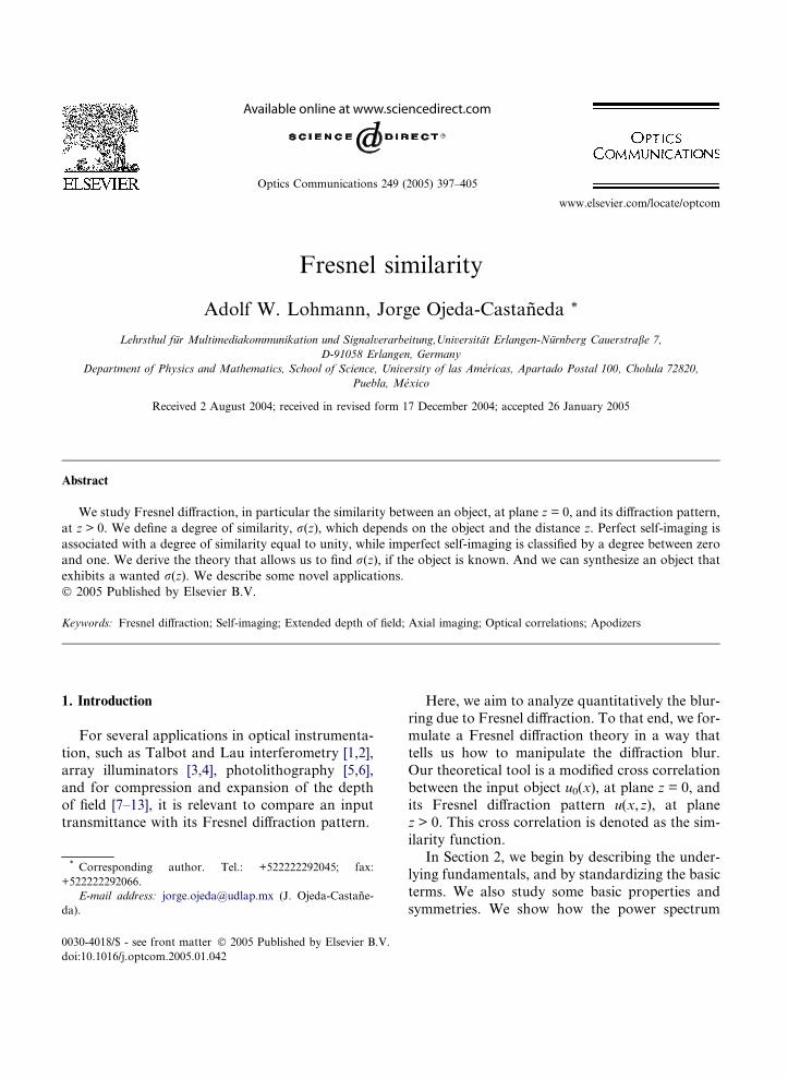
(b)

Fig. 1. Optical setup for: (a) Fresnel diffraction with input

object u0(x), and Fresnel diffraction pattern u(x,z), (b) the

optical setup for measuring the similarity function. A pinhole at

the rear focal plane of the last lens implements the integration

of the product uðx; zÞu�0ðxÞ.

2. Underlying fundamentals

The optical setup that we have in mind is de-

picted in Fig. 1(a). A monochromatic plane wave

illuminates the object with complex amplitude

transmission u0(x). The second transversal coordi-nate y is of no interest for now. The complex

amplitude distribution, u(x, z), just behind the ob-

ject (at z = 0) is

uðx; 0Þ ¼ u0ðxÞ: ð1Þ

The complex amplitude in Eq. (1) acts as the refer-

ence signal for the definition of similarity functionas

SðzÞ ¼Z 1

�1uðx; zÞu�ðx; 0Þdx

¼Z 1

�1uðx; zÞu�0ðxÞdx; ð2Þ

where the limits of integration are ±1 for ape-

riodic objects and quasi-periodic objects, while

the limits are ±d/2 for periodic objects with per-

iod d.

In Fig. 1(b), we show an optical setup for imple-

menting the operation in Eq. (2) by using twomasks. In Section 6, we discuss other approaches

for evaluating the similarity function with a single

mask.

It is important to note that the value of the sim-ilarity function at the object plane, S(0), is the total

energy of the optical signal, which is a finite num-

ber. That is, we consider optical signals that are

bounded either in the space domain (windowed

signals), or in the frequency domain (band-limited

signals). In mathematical terms,

A.W. Lohmann, J. Ojeda-Castaneda / Optics Communications 249 (2005) 397–405 399

Sð0Þ ¼Z 1

�1juðx; 0Þj2 dx ¼

Z 1

�1ju0ðxÞj2 dx

¼Z 1

�1j~u0ðvÞj2 dv ¼ E: ð3Þ

Next, we show that when dealing with optical sig-

nals that are infinitely extended, the bias term must

be zero. That is, if

u0ðxÞ ¼ ½hui þ DuðxÞ�; ð4Þ

with

hui ¼Z 1

�1u0ðxÞdx; ð5Þ

then, the condition in Eq. (3) implies that

E ¼Z 1

�1½jhuij2 þ jDuðxÞj2 þ 2Refhui�DuðxÞg�dx:

ð6ÞAnd therefore, to avoid an undefined value, we

must set

hui ¼Z 1

�1u0ðxÞdx ¼ 0; ð7Þ

and consequently

E ¼Z 1

�1jDuðxÞj2 dx: ð8Þ

Now, if the definition of similarity, in Eq. (1), is

normalized to stay within unity, 0 6 |r(z)| 6 1, wespeak of the ‘‘degree of similarity’’. For this pur-

pose we divide the original S(z) by S(0) = E. That

is, since |S(z)| 6 S(0) then

rðzÞ ¼ SðzÞ=Sð0Þ: ð9Þ

In Sections 3 and 4, we show that for quasi-

periodic and periodic signals the similarity func-tion is a periodic function, and that the degree of

similarity has the following property: r(nZT) =

r(0) = 1, where n is an integer number, and

zT = 2d2/k is the so-called Talbot distance.

Next, we recognize first that for the input

u0ðxÞ ¼Z 1

�1~u0ðvÞ expði2pxvÞdv; ð10Þ

its Fresnel diffraction pattern can be expressed in

terms of a Fourier transform as follows

uðx; zÞ ¼Z 1

�1~u0ðvÞ exp½i2pz

pðk�2 � v2Þ�

� expði2pxvÞdv: ð11Þ

Since in the paraxial regime one can approximatep(k�2�v2) � k�1 � k v2/2 then except for the

phase factor exp(i2pz/k), in the paraxial approxi-

mation equation (11) reduces to

uðx; zÞ ¼Z 1

�1~u0ðvÞ expð�ipkzv2Þ expði2pxvÞdv:

ð12Þ

Then, by substituting either Eq. (11) or Eq. (12) inEq. (2), one has that

SðzÞ ¼Z 1

�1j~u0ðvÞj2 exp½i2pz

Z 1

�1ðk�2 � v2Þ�dv

ð13Þ

or, except for the phase factor exp(i2pz/k), that inthe paraxial regime

SðzÞ ¼Z 1

�1j~u0ðvÞj2 expð�ipkzv2Þdv: ð14Þ

It is apparent from Eqs. (13) and (14) that the sim-ilarity function describes the Fresnel propagation

of the power spectrum |u0(v)|2.

The proposed measurement of similarity is

independent of the phase of the Fourier spectrum

u0(v). It is surprising because S(z) is not an auto-

correlation, but a cross correlation of two different

functions u(x, 0) and u(x, z).

We recognize that another important feature, ofEqs. (10) and (11), is that they allow for designing

similarity values by proper selection of the power

spectrum |u0(v)|2. A similar problem occurs when

synthesizing the optical transfer function by using

computer-generated holography; as is discussed in

Section 7.

Either from Eq. (13), or from Eq. (14), we can

identify the following symmetry

SðzÞ ¼ S�ð�zÞ: ð15Þ

In other words, the similarity function is a hermi-tian function both in the paraxial approximation

and beyond the paraxial approximation. Eq. (15)

also shows that |S(z)| 6 S(0).


We note also that the similarity function remains

invariant under the following transformations:

(a) S(z) does not change if one displaces later-

ally the input, namely

u0ðxÞ ! u0ðx� x0Þand

uðx; zÞ ! uðx� x0; zÞ:Since

~u0ðv; x0Þ ! ~u0ðvÞ expð�i2pvx0Þand

~uðv; x0Þ ! ~uðvÞ expð�i2pvx0Þ expð�ipkzv2Þ:Thus,

Sðz; x0Þ ¼Z 1

�1j~u0ðv; x0Þj2 expð�ipkzv2Þdv ¼ SðzÞ:

ð16Þ(b) If one takes the complex conjugate of the in-

put, namely

u0ðxÞ ! u�0ðxÞ;then

~u0ðvÞ ! ~u�0ð�vÞ;and then for the paraxial regime

SðzÞ ¼Z 1

�1j~u�0ð�vÞj2 expð�ipkzv2Þdv ¼ S�ð�zÞ:

ð17Þ(c) If one displaces longitudinally, say by z0, the

input as well as the second mask the function S(z)

does not change

u0ðx; z ¼ 0Þ ! u0ðx; z0Þ; and uðx; zÞ ! uðx; zþ z0Þ:ð18Þ

In other words, the similarity function depends

only on the difference of the axial coordinate z.

The similarity function is next applied in thefollowing sections, for analyzing some illustrative

cases.

3. Aperiodic objects

A general treatment of aperiodic objects is be-

yond our present scope. Here, we discuss a simple

example, within the paraxial approximation,

which illustrates the concept of similarity.

We consider a suitably modified Gaussian

beam. Its power spectrum is

j~u0ðvÞj2 ¼ jvj expð�pv2=a2Þ: ð19ÞThe scaling factor a�2 defines the width of the

Gaussian beam. For this example, if one considers

that z � k, then the similarity function is

SðzÞ ¼Z Na

�Najvj exp½�pða�2 þ ikzÞv2�dv;

SðzÞ ¼ 1=2

Z N2a2

0

exp½�pða�2 þ ikzÞv2�dðv2Þ

þ 1=2

Z N2a2

0

exp½�pða�2 þ ikzÞv2�dðv2Þ;

¼Z N2a2

0

exp½�pða�2 þ ikzÞv2�dðv2Þ:

ð20ÞIn Eq. (20) we set the upper limit equal to (Na)2

where N is a large integer number, such that

exp(�pN2)� 1. Then, within the approximation

that z � k, it is straightforward to evaluate Eq.

(20) to obtain

SðzÞ � 1=½a�2 þ ikz� � ½a�2 � ikz�=½a�4 þ k2z2�:ð21Þ

Now, since S(0) = a2 then the modulus of the de-

gree of similarity can be written as

jrðzÞj � 1=pð1þ a4k2z2Þ: ð22Þ

Eq. (22) represents a monotonically decreasing

function.

4. Quasi-periodic objects

Quasi-periodic objects have a power spectrumof the form

j~u0ðvÞj2 ¼ ð1=MÞXM�1

m¼0

jamj2d½v� vm�: ð23Þ

A subset of these quasi-periodic objects is the setof ‘‘Montgomery objects’’. Their power spectrum

peaks are located at


vm ¼ v1pm; and v1 ¼ 1=d: ð24Þ

We denote aspm the square root of m. Montgom-

ery identified this set, when describing the neces-

sary and sufficient conditions for self-imaging

[14]. The similarity function for the ‘‘Montgomery

objects’’ is

SðzÞ ¼ ð1=MÞXM�1

m¼0

jamj2 expð�ipkzm=d2Þ

¼ ð1=MÞXM�1

m¼0

jamj2 expð�i2pzm=ZTÞ; ð25Þ

which is to be recognized as a finite Fourier serieswith fundamental period equal to the Talbot

length ZT = 2d2/k. Hence, the similarity function,

as well as the degree of similarity, is a periodic

function. In mathematical terms,

rðzÞ ¼XM�1

m¼0

jamj2 exp �i2pzm=ZTð Þ" #,XM�1

m¼0

jamj2

ð26Þis a periodic function

rðzþ nZTÞ ¼ rðzÞ; ð27Þwith fundamental period ZT. Specifically, for

z = 0, we have that r(n ZT) = r(0) = 1.

We discuss next the behavior of the similarity

function at fractions; say 1/M, of the Talbot

length. Since we assume that z = n(ZT/M), forn = 0,1,2,. . .,M � 1, then Eq. (25) becomes

SðnZT=MÞ ¼ ð1=MÞXM�1

m�0

jamj2 expð�i2pmn=MÞ;

ð28Þwhich is to be recognized as the finite Fourier

transform of the coefficients |am|2. And therefore,

if the finite Fourier transform of the coefficient

am is the coefficient An,

An ¼ ð1=MÞXM�1

m�0

am expð�i2pmn=MÞ; ð29Þ

then the similarity function in Eq. (28) can be writ-

ten as the autocorrelation of the Am coefficients.

That is,

SðnZT=MÞ ¼XM�1

m�0

A�mAmþn: ð30Þ

A nice application of Eq. (30) is the so-called

pseudo-random sequence. By using a pseudo-ran-

dom sequence for Am one can shape (SnZT/M) to

be equal to 1 only if n = 0 and multiple numbers

of M. Otherwise S(nZT/M) should be equal tozero. And consequently, the degree of similarity

can be manipulated to be a Dirac�s comb, with per-

iod ZT. Next, we discuss the periodic case.

5. Periodic structures

Optical gratings are good examples of periodicinputs. Their power spectrum is represented by

j~u0ðvÞj2 ¼X1

m¼�1jamj2d½v� m=d�: ð31Þ

In Eq. (31) we disregard the evanescent waves by

limiting the summation index m to |m|<d/k = M.

In other words, we restrict the term ‘‘similarity’’

to distances beyond the reach of evanescent waves.

Often the grating may deflect only into a narrow

angular range |sinam|. In that case the z-dependent

part of the exponent (1 � cosa)z/k maybe approx-imated by (z/2k)sin2am = m2kzv2/2. In other words,

we invoke the paraxial approximation that simpli-

fies the analysis.

Hence, within the paraxial regime, the similarity

function is the finite Fourier series

SðzÞ ¼XMm¼�M

jamj2 expð�ipkzm2=d2Þ;

¼XMm¼�M

jamj2 expð�i2pzm2=ZTÞ: ð32Þ

We note that Eq. (32) agrees well with the predic-

tion made on symmetries in Eq. (15). Again, as in

the case of the ‘‘Montgomery objects’’, for a peri-

odic input the degree of similarity is unity at the

self-imaging planes, as was expected.

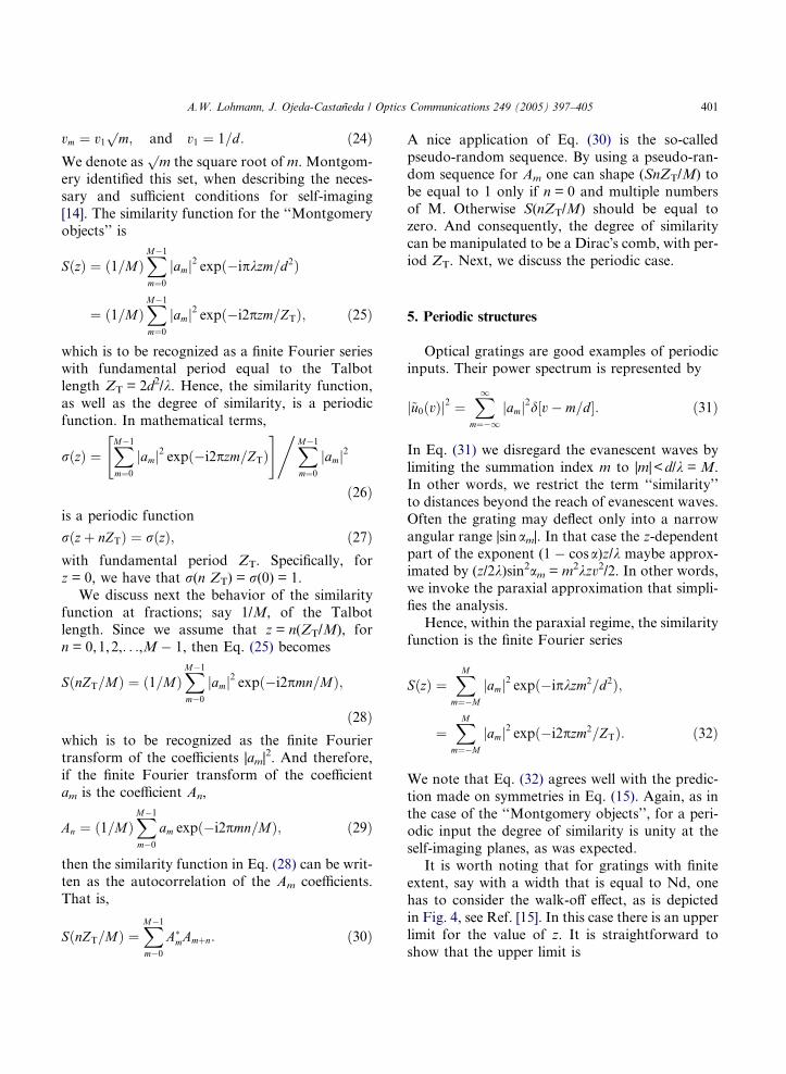
It is worth noting that for gratings with finiteextent, say with a width that is equal to Nd, one

has to consider the walk-off effect, as is depicted

in Fig. 4, see Ref. [15]. In this case there is an upper

limit for the value of z. It is straightforward to

show that the upper limit is

u0(x)

z0

.dx |.|2ADD

z + z(a)

(b)

0


Z ¼ Nðd2=kÞp½1� ðk=dÞ2�Z¼ ½MN

pð1�M�2Þ�d: ð33Þ

If one neglects the diffraction produced by the fi-

nite size of the grating, then at z = Z the non-zero

diffracting orders have left the transverse region of

interest. Under these conditions, the degree of sim-

ilarity is equal to unity. However, roughly speak-

ing, the walk-off effect is harmless if the numbers

of grating periods is much larger than the numberof diffraction orders.

u(x,z+z0)

z0

u0(x) u0(x,z0)

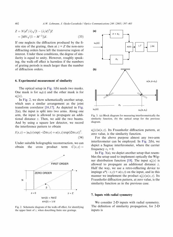
Fig. 3. (a) Block diagram for measuring interferometrically the

similarity function, (b) the optical setup for the previous

diagram.

6. Experimental measurement of similarity

The optical setup in Fig. 1(b) needs two masks.

One mask is for u0(x) and the other mask is for

u�0ðxÞ.In Fig. 2, we show schematically another setup,

which uses a similar arrangement as the joint

transform correlator [16,17]. As depicted in Fig.

2(a), the input is split into two arms. Along one

arm, the input is allowed to propagate an addi-

tional distance z. Then, we add the two beams.

And by using a square law detector, we record

the interference pattern to obtain

Iðx; zÞ ¼ ju0ðxÞexpð�i2pv1xÞþ uðx; zÞexpði2pv1xÞj2:ð34Þ

Under suitable holographic reconstruction, we can

obtain the cross product term Cðx; zÞ ¼

FIRST ORDER

ZERO ORDER

N

z = 0 z = Z

tan(β

β

) = Nd/Z

sin(β) = λ/d

Fig. 2. Schematic diagram of the walk-off effect, for identifying

the upper limit of z, when describing finite size gratings.

u�0ðxÞuðx; zÞ. Its Fraunhofer diffraction pattern, at

zero value, is the similarity function.For the above purpose almost any two-arm

interferometer can be employed. In Fig. 2(b), we

depict a Sagnac interferometer, where the carrier

frequency v1 = 0.

In Fig. 3(a), we depict another setup that resem-

bles the setup used to implement optically the Wig-

ner distribution function [18]. The input u�0ðxÞ is

allowed to propagate an additional distance z.Half the way, we use a retro-reflecting device to

impinge u*(�x,z) = u(x,z) on the input, and in this

manner we implement the product u�0ðxÞuðx; zÞ. ItsFraunhofer diffraction pattern, at zero value, is the

similarity function as in the previous case.

7. Inputs with radial symmetry

We consider 2-D inputs with radial symmetry.

The definition of similarity propagation, for 2-D

inputs is

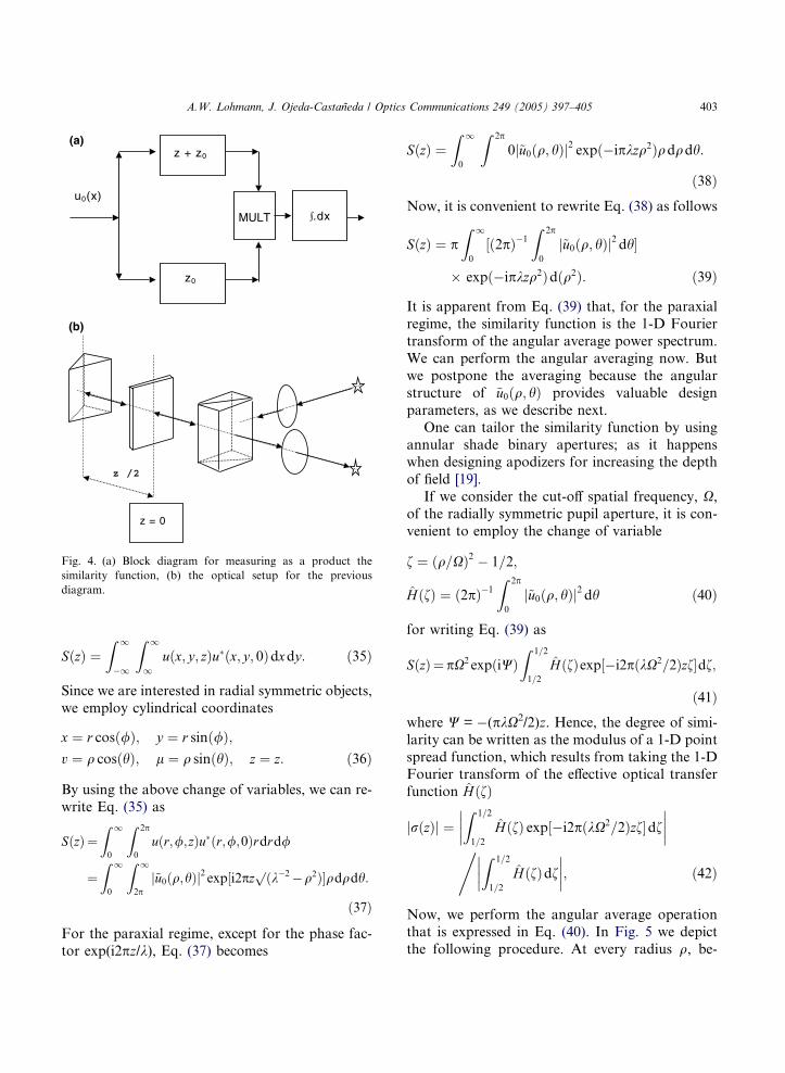
u0(x)

.dxMULT

z0

z + z(a)

(b)

0

z = 0

Fig. 4. (a) Block diagram for measuring as a product the

similarity function, (b) the optical setup for the previous

diagram.


SðzÞ ¼Z 1

�1

Z 1

1uðx; y; zÞu�ðx; y; 0Þdxdy: ð35Þ

Since we are interested in radial symmetric objects,

we employ cylindrical coordinates

x ¼ r cosð/Þ; y ¼ r sinð/Þ;v ¼ q cosðhÞ; l ¼ q sinðhÞ; z ¼ z: ð36Þ

By using the above change of variables, we can re-

write Eq. (35) as

SðzÞ¼Z 1

0

Z 2p

0

uðr;/;zÞu�ðr;/;0Þrdrd/

¼Z 1

0

Z 1

2pj~u0ðq;hÞj2 exp½i2pz

pðk�2�q2Þ�qdqdh:

ð37Þ

For the paraxial regime, except for the phase fac-

tor exp(i2pz/k), Eq. (37) becomes

SðzÞ ¼Z 1

0

Z 2p

0j~u0ðq; hÞj2 expð�ipkzq2Þqdqdh:

ð38ÞNow, it is convenient to rewrite Eq. (38) as follows

SðzÞ ¼ pZ 1

0

½ð2pÞ�1

Z 2p

0

j~u0ðq; hÞj2 dh�

� expð�ipkzq2Þdðq2Þ: ð39Þ

It is apparent from Eq. (39) that, for the paraxial

regime, the similarity function is the 1-D Fourier

transform of the angular average power spectrum.

We can perform the angular averaging now. But

we postpone the averaging because the angular

structure of ~u0ðq; hÞ provides valuable design

parameters, as we describe next.

One can tailor the similarity function by usingannular shade binary apertures; as it happens

when designing apodizers for increasing the depth

of field [19].

If we consider the cut-off spatial frequency, X,of the radially symmetric pupil aperture, it is con-

venient to employ the change of variable

f ¼ ðq=XÞ2 � 1=2;

HðfÞ ¼ ð2pÞ�1

Z 2p

0

j~u0ðq; hÞj2 dh ð40Þ

for writing Eq. (39) as

SðzÞ¼ pX2 expðiWÞZ 1=2

1=2

HðfÞexp½�i2pðkX2=2Þzf�df;

ð41Þwhere W = �(pkX2/2)z. Hence, the degree of simi-

larity can be written as the modulus of a 1-D point

spread function, which results from taking the 1-DFourier transform of the effective optical transfer

function HðfÞ

jrðzÞj ¼Z 1=2

1=2

HðfÞ exp½�i2pðkX2=2Þzf�df��

��, Z 1=2

1=2

HðfÞdf��

��; ð42Þ

Now, we perform the angular average operation

that is expressed in Eq. (40). In Fig. 5 we depict

the following procedure. At every radius q, be-

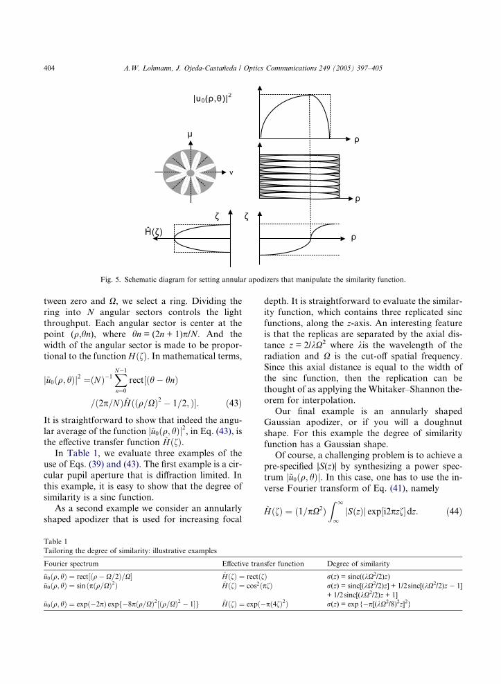
Fig. 5. Schematic diagram for setting annular apodizers that manipulate the similarity function.


tween zero and X, we select a ring. Dividing the

ring into N angular sectors controls the light

throughput. Each angular sector is center at the

point (q,hn), where hn = (2n + 1)p/N. And the

width of the angular sector is made to be propor-

tional to the function HðfÞ. In mathematical terms,

j~u0ðq; hÞj2 ¼ðNÞ�1XN�1

n¼0

rect½ðh� hnÞ

=ð2p=NÞHððq=XÞ2 � 1=2; Þ�: ð43Þ

It is straightforward to show that indeed the angu-

lar average of the function j~u0ðq; hÞj2, in Eq. (43), is

the effective transfer function HðfÞ.In Table 1, we evaluate three examples of the

use of Eqs. (39) and (43). The first example is a cir-

cular pupil aperture that is diffraction limited. In

this example, it is easy to show that the degree of

similarity is a sinc function.

As a second example we consider an annularly

shaped apodizer that is used for increasing focal

Table 1

Tailoring the degree of similarity: illustrative examples

Fourier spectrum Effective tran

~u0ðq; hÞ ¼ rect½ðq� X=2Þ=X� HðfÞ ¼ rectðf~u0ðq; hÞ ¼ sin ðpðq=XÞ2Þ HðfÞ ¼ cos2ð

~u0ðq; hÞ ¼ expð�2pÞ expf�8pðq=XÞ2½ðq=XÞ2 � 1�g HðfÞ ¼ expð�

depth. It is straightforward to evaluate the similar-

ity function, which contains three replicated sinc

functions, along the z-axis. An interesting feature

is that the replicas are separated by the axial dis-

tance z = 2/kX2 where kis the wavelength of the

radiation and X is the cut-off spatial frequency.Since this axial distance is equal to the width of

the sinc function, then the replication can be

thought of as applying the Whitaker–Shannon the-

orem for interpolation.

Our final example is an annularly shaped

Gaussian apodizer, or if you will a doughnut

shape. For this example the degree of similarity

function has a Gaussian shape.Of course, a challenging problem is to achieve a

pre-specified |S(z)| by synthesizing a power spec-

trum j~u0ðq; hÞj. In this case, one has to use the in-

verse Fourier transform of Eq. (41), namely

HðfÞ ¼ ð1=pX2ÞZ 1

1jSðzÞj exp½i2pzf�dz: ð44Þ

sfer function Degree of similarity

Þ r(z) = sinc((kX2/2)z)

pfÞ r(z) = sinc[(kX2/2)z] + 1/2sinc[(kX2/2)z � 1]

+ 1/2sinc[(kX2/2)z + 1]

pð4fÞ2Þ r(z) = exp{�p[(kX2/8)2z]2}


And since from Eq. (15) we know that

S(z) = S*(�z) then HðfÞ is a real function. Hence,

by properly selecting the angular widths one can

synthesis HðfÞ.

8. Final remarks

We have proposed to measure the similarity of

a complex amplitude transmittance with its Fres-

nel diffraction pattern, at a distance z, by the use

of a modified cross correlation, which is denoted

as the similarity function S(z) = S*(�z).We have described schematically three types of

experimental setups for experimentally evaluating

S(z). For the first type, the optical setup uses two

masks, one mask for u0(x) and the other mask

for u�0ðxÞ. In the second type, we use the experi-

mental scheme of the joint transform correlation.

A convenient interference pattern is recorded,

and under holographic reconstruction we obtainthe similarity function. In the third type, we take

advantage of the symmetry properties of real

transmittance objects to implement the product

with a retro-reflecting device.

We have shown that under the paraxial regime,

the similarity function is the Fresnel diffraction

pattern of the power spectrum. For radially sym-

metric objects the similarity function can be ex-pressed as the 1-D Fourier transform of the

angular average power spectrum.

We have discussed specific applications that

illustrate the use of this concept. Specifically, we

have shown that for certain apodized Gaussian

beams the similarity function can be a monotoni-

cally decreasing function.

We have indicated that for certain quasi-peri-odic objects, as well as for periodic structures,

the degree of similarity is periodic function with

fundamental period equal to the Talbot length.

The degree of similarity can be shaped as a comb

function by using quasi-periodic structures related

to the pseudo-random sequences. For periodic ob-

jects with finite extension, we employ the concept

of the walk-off effect to identify the upper limitof z.

We have shown that for diffraction limited

apertures the degree of similarity is a sinc function.

We have discussed that certain apodizers can ex-

tend the depth of focus, by replicating the sinc

function along the z-axis. Since the replicated sinc

functions are separated axially by the sinc width,

then the depth of focus increases following theWhitaker–Shannon interpolation formula.

Finally, we have shown how to synthesize a

similarity function by means of binary screens with

angular sectors.

Acknowledgements

We are grateful to the reviewers for their helpful

suggestions. One of us (J.O.C.) is indebted to the

Alexander von Humboldt Foundation for finan-

cial support.

References

[1] A.W. Lohmann, D. Silva, Opt. Commun. 2 (1971) 413.

[2] H.O. Bartelt, J. Jahns, Opt. Commun. 30 (1979) 268.

[3] A.W. Lohmann, Optik 79 (1988) 41.

[4] M. Testorf, V. Arrizon, J. Ojeda-Castaneda, J. Opt. Soc.

Am. A 16 (1999) 97.

[5] B. Salik, J. Rosen, A. Yariv, J. Opt. Soc. Am. A 12 (1995)

1702.

[6] J.E. Harvey, A. Krywono, D. Bogunovic, Appl. Opt. 44

(2002) 2586.

[7] J. Ojeda-Castaneda, Pedro Andres, M. Martinez-Corral,

Appl. Opt. 33 (1994) 7611.

[8] J. Ojeda-Castaneda, P. Andres, A. Dıaz, Opt. Lett. 5

(1986) 1233.

[9] J. Ojeda-Castaneda, L.R. Berriel-Valdos, Appl. Opt. 27

(1988) 790.

[10] E.R. Dowski, T.W. Cathey, Appl. Opt. 34 (1995) 1859.

[11] S. Mezouari, A.A. Harvey, Opt. Lett. 28 (2003) 771.

[12] N. George, W. Chi, J. Opt. Pure Appl. 5 (2003) s157.

[13] A. Castro, J. Ojeda-Castaneda, Appl. Opt. 43 (2004) 3474.

[14] W.D. Montgomery, J. Opt. Soc. Am. 57 (1967) 772.

[15] A.W. Lohmann, Optical Information Processing, page 107,

Multimediakommunikation und Signalverarbeitung,

Erlangen-Nurnberg University, Cauerstrasse 7, D-91058

Erlangen, Germany Erlangen, 1978.

[16] C.S. Weaver, J.W. Goodman, Appl. Opt. 5 (1966) 1248–

1249.

[17] J.E. Rau, J. Opt. Soc. Am. 56 (1966) 1490.

[18] K.-H. Brenner, A.W. Lohmann, Opt. Commun. 42 (1982)

310.

[19] A.W. Lohmann, J. Ojeda-Castaneda, A. Serrano-Heredia,

Appl. Opt. 34 (1998) 317.

Fresnel diffraction of substructured gratings

Documents

Transcript of Fresnel diffraction of substructured gratings