Tensor Alignment Based Domain Adaptation for Hyperspectral ...

JOURNAL OF LATEX CLASS FILES, VOL. 14, NO. 8, AUGUST 2015 1

Tensor Alignment Based Domain Adaptation forHyperspectral Image Classification

Yao Qin, Student Member, IEEE, Lorenzo Bruzzone, Fellow, IEEE, and Biao Li

Abstract—This paper presents a tensor alignment (TA) baseddomain adaptation method for hyperspectral image (HSI) classi-fication. To be specific, HSIs in both domains are first segmentedinto superpixels and tensors of both domains are constructed toinclude neighboring samples from single superpixel. Then we con-sider the subspace invariance between two domains as projectionmatrices and original tensors are projected as core tensors withlower dimensions into the invariant tensor subspace by applyingTucker decomposition. To preserve geometric information in orig-inal tensors, we employ a manifold regularization term for coretensors into the decomposition progress. The projection matricesand core tensors are solved in an alternating optimization mannerand the convergence of TA algorithm is analyzed. In addition,a post-processing strategy is defined via pure samples extractionfor each superpixel to further improve classification performance.Experimental results on four real HSIs demonstrate that theproposed method can achieve better performance compared withthe state-of-the-art subspace learning methods when a limitedamount of source labeled samples are available.

Index Terms—Domain adaptation (DA), hyperspectral image(HSI) classification, superpixel segmentation, tensor alignment

I. INTRODUCTION

IN THE past decades, extensive research efforts have beenspent on hyperspectral remote sensing since hyperspec-

tral data contains detailed spectral information measured incontiguous bands of the electromagnetic spectrum [1]–[3].Due to the discriminative spectral information of such data,they have been used for a wide variety of applications,including agricultural monitoring [4], mineral exploration [5],and etc. One fundamental challenge in these applications ishow to generate accurate land-cover maps. Although super-vised learning for hyperspectral image (HSI) classification hasbeen extensively developed in the literature (including randomforest [6], support vector machine (SVM) [7], laplacian SVM(LapSVM) [8]–[10], decision trees [11] and support tensor ma-chine (STM) [12]), sufficient labeled training samples shouldbe available to obtain satisfactory classification results. Thiswould require extensive and expensive field data collectioncompaigns. Furthermore, with the advance of newly-developedspaceborne hyperspectral sensors, large numbers of HSIs are

Manuscript received September 4, 2018. (Corresponding author: LorenzoBruzzone.)

Y. Qin is with the College of Electronic Science, National University ofDefense Technology, Changsha 410073, China and Department of InformationEngineering and Computer Science, University of Trento, 38122 Trento, Italy(e-mail: [email protected]).

L. Bruzzone is with Department of Information Engineering andComputer Science, University of Trento, 38122 Trento, Italy (e-mail:[email protected]).

B. Li is with the College of Electronic Science, National University ofDefense Technology, Changsha 410073, China.

easily collected and it is not feasible to timely label sam-ples of the hyperspectral images as reference for training.Therefore, only limited labeled samples are available in mostreal applications of hyperspectral classification. Accordingto the statistical theory in supervised learning, the data tobe classified are expected to follow the same probabilitydistribution function (PDF) of training data. However, sincethe physical conditions (i.e. illumination, atmosphere, sensorparameters, and etc.) can hardly be the same when collectingdata, PDFs of training and testing data tend to be different(but related) [13]. Then how to apply the labeled samples oforiginal HSI to the related HSI is challenging in such cases.These problems can be addressed by adapting models trainedon a limited number of source samples (source domain) tonew but related target samples (target domain). The problemshould be further studied for the development of hyperspectralapplications.

According to the machine learning and pattern recognitionliterature, the problem of adapting model trained on a sourcedomain to a target domain is referred to as transfer learningor domain adaptation (DA) [13]. The main idea of transferlearning is to adapt the knowledge learned in one task to arelated but different task. An excellent review of transfer learn-ing can be found in [14], [15]. In general, transfer learning isdivided into four categories based on the properties of domainsand tasks, i.e. DA, multi-task learning, unsupervised transferlearning and self-taught learning. In fact, DA has greaterimpact on practical applications. When applied to classificationproblems, DA aims to generate accurate classification resultsof target samples by utilizing the knowledge learned on thelabeled source samples. According to [3], DA techniques forremote sensing applications can be roughly categorized asselection of invariant features, adaptation of data distributions,adaptation of classifier and adaptation of classifier by activelearning (AL).

In our case of HSI classification, we focus on the sec-ond category, i.e. adaptation of data distributions, in whichdata distributions of both domains are made as similar aspossible to keep the classifier unchanged. Despite the factthat several DA methods have been proposed for HSI clas-sification, they treat HSIs as several single samples, whichrenders them incapable of reflecting and preserving importantspatial consistency of neighboring samples. In this paper, toexploit the spatial information in a natural and efficient way,tensorial processing is utilized, which treats HSIs as three-dimensional (3D) tensors. Tensor arithmetic is a generalizationof matrix and vector arithmetic, and is particularly well suitedto represent multilinear relationships that neither vector normatrix algebra can capture naturally [16], [17]. The power of

arX

iv:1

808.

0976

9v2

[ee

ss.I

V]

4 S

ep 2

018


tensorial processing for improving classification performancewithout DA has been proved in [18]–[22]. Similarly, whenwe apply tensorial processing to HSI in DA, multilinearrelationships between neighboring samples in both HSIs arewell captured and preserved, while conventional DA methodsusing vectorization deal with single samples. Tensor-based DAmethods for visual application has demonstrated the efficacyand efficiency on the task of cross-domain visual recognition[17], [23], whereas there are few published works on DA byusing tensorial processing of HSIs.

To be specific, we propose a tensor alignment (TA) methodfor DA, which can be divided into two steps. First, theoriginal HSI data cubes in both domains are divided into smallsuperpixels and each central sample is represented as a 3Dtensor consisting of samples in the same superpixel. In thisway, each tensor is expected to include more samples fromthe same class. Since tensors are acted as “basic elements” inthe TA method, we believe that high purity of tensors bringsbetter adaptation performance. Second, taking into account thecomputational cost, we randomly select part of target tensors inthe progress of TA to identify the invariance subspace betweenthe two domains as projection matrices. This is done on thesource and selected target tensors, and the subspace sharedby both domains is obtained by utilizing three projectionmatrices {U(1),U(2),U(3)} with original geometry preserved.The solution is addressed through the Tucker decomposition[24] with orthogonal regularization on projection matrices andoriginal tensors are represented by core tensors in the sharedsubspace. Fig. 1 illustrates the manifold regularized TA methodwith a 1-Nearest Neighbor (1NN) geometry preserved.

In addition to the TA method, after generating classificationmap, a post-processing strategy based on pure samplesextraction of each superpixel is employed to improveperformances. The pure samples in superpixels have similarspectral features and likely belong to the same class.Therefore, if most pure samples in a superpixel are classifiedas i-th class, it is probable that the remaining pure samplesbelongs to the same class. Since samples in one superpixelmay belong to two or even more classes and there arealways classification errors in DA, the ratio of pure samplespredicting as the same class might be reduced if we extractmore pure samples. Therefore, we extract the pure samplesby fixing the ratio as 0.7. Specifically, final pure samples areextracted by first projecting samples in each superpixel toprincipal component axis and then including more samples inthe middle range of the axis till the ratio reaches 0.7. In thisway the consistency of classification results on pure samplesis enforced. To sum up, the main contributions of our worklie in the following two aspects:• We propose a manifold regularized tensor alignment (TA)

for DA and develop the corresponding efficient iterativealgorithm to find the solutions. Moreover, we analyze theconvergence properties of the proposed algorithm and itscomputational complexity as well.• We introduce a pure samples extraction strategy as post-

processing to further improve the classification performance.Comprehensive experiments on four publicly availablebenchmark HSIs have been conducted to demonstrate the

Source Subspace

Shared SubspaceTarget Subspace

U(1)

U(2)

U(3)

Fig. 1. Illustration of the manifold regularized tensor alignment method.There are 5 tensor objects for each class in the source domain, while 3 tensorobjects for each class in the target domain. The shared subspace is obtainedby utilizing 3 projection matrices {U(1),U(2),U(3)} with original geometrypreserved. Each arrow represents the 1NN relationship between tensors. Bestview in colors.

effectiveness of the proposed algorithm.The rest of the paper is organized as follows. Related

works on adaptation of data distributions, tensorial processingof HSI and multilinear algebra are illustrated in Section II.The proposed methodology of TA is presented in section III,while the pure samples extraction strategy for classificationimprovement is outlined in Section IV. Section V describesthe experimental datasets and setup. Results and discussionsare presented in Section VI. Section VII summarizes thecontributions of our research.

II. RELATED WORK

This section briefly describes important studies related tothe adaptation of data distributions, tensorial processing ofhyperspectral data and basic concepts in multilinear algebra.

A. Adaptation of Data Distributions

Several methods for the adaptation of data distributionsfocus on subspace learning, where projected data from bothdomains are well aligned. Then, the same classifier (or re-gressor) is expected to be suitable for both domains. In [25],the data alignment is achieved through principal componentanalysis (PCA) or kernel PCA (KPCA). In [26], a PCA-basedsubspace alignment (SA) algorithm is proposed, where thesource subspace is aligned as close as possible to the targetsubspace using a matrix transformation. In [17], features fromconvolutional neural network are treated as tensors and theirinvariant subspace is obtained through the Tucker decom-position. In [27], the authors align domains with canonicalcorrelation analysis (CCA) and then perform change detection.The approach is extended to a kernel and semisupervisedversion in [28], where the authors perform change detectionwith different sensors. In [29], the supervised multi-viewcanonical correlation analysis ensemble is presented to addressheterogeneous domain adaptation problems.


A few studies assume that data from both domains lie onthe Grassmann manifold, where data alignment is conducted.In [30], the sampling geodesic flow (SGF) method is intro-duced and finite intermediate subspaces are sampled alongthe geodesic path connecting the source subspace and thetarget subspace. Geodesic flow kernel (GFK) method in [31]models infinite subspaces in the way of incremental changesbetween both domains. Along this line, GFK support vectormachine in [32] shows the performance of GFK in nonlinearfeature transfer tasks. A GFK-based hierarchical subspacelearning strategy for DA is proposed in [33], and an iterativecoclustering technique applied to the subspace obtained byGFK is proposed in [34].

Other studies hold the view that the subspace of both do-mains can be low-rank reconstructed or clustered. The recon-struction matrix is enforced to be low-rank and a sparse matrixis used to represent noise and outliers. In [35], a robust domainadaptation low-rank reconstruction (RDALRR) method is pro-posed, where a transformed intermediate representation of thesamples in the source domain is linearly reconstructed by thetarget samples. In [36], the low-rank transfer subspace learning(LTSL) method is proposed where transformations are appliedfor both domains to resolve disadvantages of RDALRR. In[37], a low-rank and sparse representation (LRSR) method ispresented by additionally enforcing the reconstruction matrixto be sparse. To obtain better results of reconstruction matrix,structured domain adaptation (SDA) in [38] utilizes block-diagonal matrix to guide iteratively the computation. Differentfrom the above methods, latent sparse domain transfer (LSDT)in [39] is inspired by subspace clustering, while the low-rank reconstruction and instance weighting label propagationalgorithm in [40] attempts to find new representations forthe samples in different classes from the source domain bymultiple linear transformations.

Other methods focus on feature extraction strategy byminimizing predefined distance measures, e.g. Maximum MeanDiscrepancy (MMD) or Bregman divergence. In [41], transfercomponent analysis (TCA) tries to learn some transfer compo-nents across domains in a Reproducing Kernel Hilbert Space(RKHS) using MMD. It is then applied to remote sensingimages in [42]. TCA is further improved by joint domain adap-tation (JDA), where both the marginal distributions and condi-tional distributions are adapted in a dimensionality reductionprocedure [43]. Furthermore, transfer joint matching (TJM)aims to reduce the domain difference by jointly matching thefeatures and reweighting the instances across domains [44].Recently, joint geometrical and statistical alignment (JGSA) ispresented by reducing the MMD and forcing both projectionmatrices to be close [45]. In [46] and [47], the authors transfercategory models trained on landscape views to aerial views forhigh-resolution remote sensing images by reducing MMD.

Different from the above category for feature extraction,several studies employ manifold learning to preserve theoriginal geometry. In [48], both domains are matched throughmanifold alignment while preserving label (dis)similarities andthe geometric structures of the single manifolds. The algorithmis extended to a kernelized version in [49]. Spatial informationof HSI data is taken into account for manifold alignment in

[50]. In [51], both local and global geometric characteristicsof both domains are preserved and bridging pairs are extractedfor alignment. In addition to manifold learning, the manifoldregularized domain adaptation (MRDA) method integrates spa-tial information and the overall mean coincidence method toimprove prediction accuracy [52]. Beyond classical subspacelearning, manifold assumption and feature extraction methods,several other approaches are proposed in the literature, suchas class centroid alignment [53], histogram matching [54] andgraph matching [55].

B. Tensorial Processing of Hyperspectral Data

A few published works of tensor-based methods have beenapplied to HSI processing to fully exploit both spatial andspectral information. The texture features of HSI at differentscales, frequencies and orientations are successfully extractedby the 3D discrete wavelet transform (3D-DWT) [56]. Thegray level co-occurrence is extended to its 3D version in [57]to improve classification performance. Tensor discriminativelocality alignment (TDLA) algorithm optimizes the discrimi-native local information for feature extraction [58], while localtensor discriminant analysis (LTDA) technique is employedin [59] for spectral-spatial feature extraction. The high-orderstructure of HSI along all dimensions is fully exploited bysuperpixel tensor sparse coding to better understand the data in[60]. Moreover, several conventional 2D methods are extendedto the 3D for HSI processing, such as the 3D extension ofempirical mode decomposition in [61], [62]. The modifiedtensor locality preserving projection (MTLPP) algorithm ispresented for HSI dimensionality reduction and classificationin [63].

C. Notations and basics of Multilinear Algebra

A tensor is a multi-dimensional array that generalizes matrixrepresentation. Vectors and matrices are first and second ordertensors, respectively. In this paper, we use lower case letters(e.g. x), boldface lowercase letters (e.g. x) and boldface capitalletters (e.g. X) to denote scalars, vectors and matrices, respec-tively. Tensors of order 3 or higher will be denoted by boldfaceEuler script calligraphic letters (e.g. X ). The operations ofKronecker product, Frobenius norm, vectorization and productare denoted by ⊗, ||·||F, vec(·) and

∏, respectively. The Tr(·)

denotes the trace of a matrix.A M-th order tensor is denoted by X ∈ RI1×···×IM . The

corresponding k-mode matricization of the tensor X , denotedby X(k), unfolds the tensor X with respect to mode k. Theoperation between tensor X and a matrix U(k) ∈ RJk×Ik

is the k-mode product denoted by X ×(k) U(k), which is atensor of size I1 × · · · × Ik−1 × Jk × Ik+1 × · · · IM . Briefly,the notion for the product of tensor with a set of projectionmatrices {U(k)}Mk=1 excluding the l-mode as:

X×(l)U(l) = X

∏k 6=l

×(k)U(k) (1)

Tucker decomposition is one of the most well-known decom-position models for tensor analysis. It decomposes a M modetensor X into a core tensor G multiplied by a set projection


matrices {U(k)}Mk=1 with the objective fuction defined asfollows:

minG,U||X − G

M∏k=1

×(k)U(k)||F (2)

where G ∈ RJ1×···×JM and U represents {U(k)}Mk=1 withU(k) ∈ RJk×Ik . For simiplicity, we denote G

∏Mk=1×(k)U

(k)

as [[G;U]].By applying the l-mode unfolding, Eq. (2) can alternatively

be written as

minG,U||X(l) −U(l)G(l)(U

(−l))T||F (3)

where G(l) denotes the l-mode unfolding of G, and U(−l) de-notes

∏k 6=l⊗U(k). The vectorization of (3) can be formulated

asminG,U||vec(X(l))− (U(−l) ⊗U(l))vec(G(l))||F (4)

Note that regularizations of G and U are ignored in aboveequations.

III. PROPOSED TENSOR ALIGNMENT APPROACH

A. Problem DefinitionAssume that we have ns tensor samples {X i

s}nsi=1 of mode

M in the source domain, where X is ∈ RI1×···×IM . Similarly,

tensors in the target domain are denoted as {X jt }

ntj=1. In this

paper, we consider only homogeneous DA problem, thus weassume that X j

t ∈ RI1×···×IM . In the context of DA, wefollow the idea to represent the subspace invariance betweentwo domains as projection matrices U = {Ul}Ml=1, whereUl ∈ RJl×Il . Intuitively, we propose to conduct subspacelearning on the tensor samples in both domains with mani-fold regularization. Fig. 1 shows that the shared subspace isobtained by utilizing 3 projection matrices {U(1),U(2),U(3)}.By performing Tucker decomposition simultaneously, the ten-sor samples in both domains are represented by the corre-sponding core tensors GS = {GiS}

nsi=1 and GT = {GiT }

nTi=1 with

smaller dimensions in the shared subspace. The geometricalinformation should be preserved as much as possible viaforcing manifold regularization during subspace learning. Inthe next subsection, we will introduce how to construct HSItensors and perform tensor subspace alignment.

B. Tensors ConstructionDA is achieved by tensor alignment, where HSI tensors

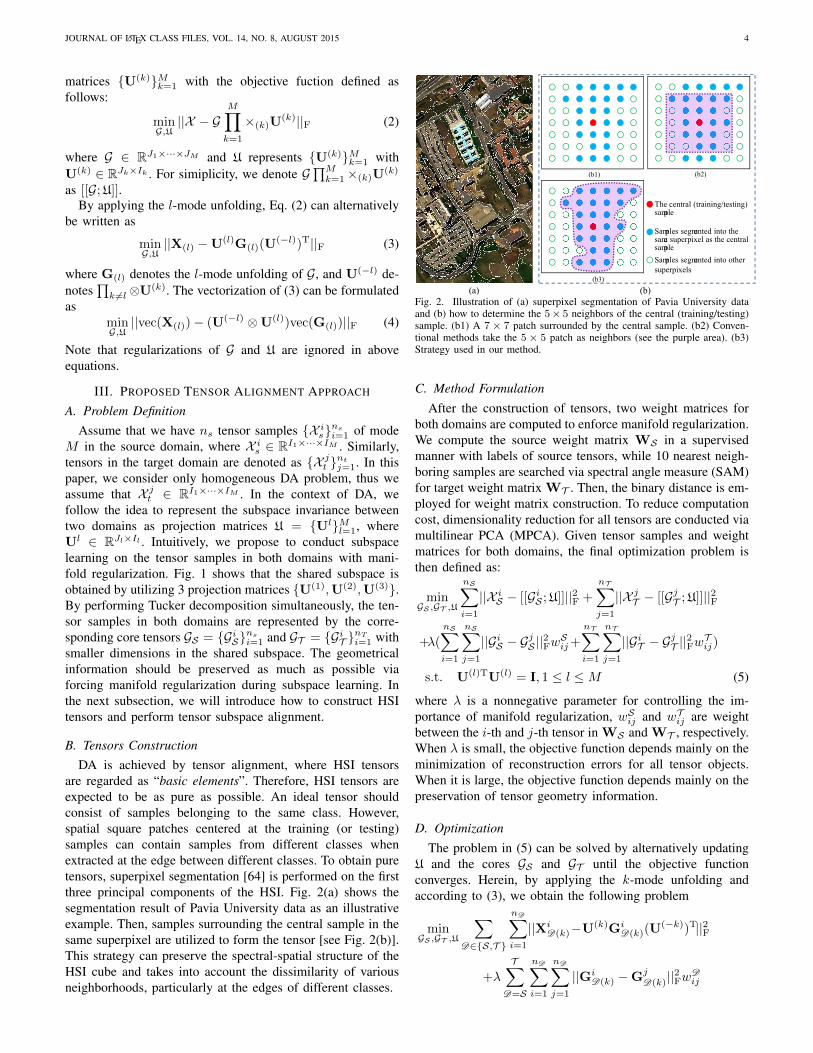
are regarded as “basic elements”. Therefore, HSI tensors areexpected to be as pure as possible. An ideal tensor shouldconsist of samples belonging to the same class. However,spatial square patches centered at the training (or testing)samples can contain samples from different classes whenextracted at the edge between different classes. To obtain puretensors, superpixel segmentation [64] is performed on the firstthree principal components of the HSI. Fig. 2(a) shows thesegmentation result of Pavia University data as an illustrativeexample. Then, samples surrounding the central sample in thesame superpixel are utilized to form the tensor [see Fig. 2(b)].This strategy can preserve the spectral-spatial structure of theHSI cube and takes into account the dissimilarity of variousneighborhoods, particularly at the edges of different classes.

(b1) (b2)

(b3)

The central (training/testing) sample

Samples segmented into the same superpixel as the central sample

Samples segmented into other superpixels

(a) (b)Fig. 2. Illustration of (a) superpixel segmentation of Pavia University dataand (b) how to determine the 5× 5 neighbors of the central (training/testing)sample. (b1) A 7× 7 patch surrounded by the central sample. (b2) Conven-tional methods take the 5× 5 patch as neighbors (see the purple area). (b3)Strategy used in our method.

C. Method Formulation

After the construction of tensors, two weight matrices forboth domains are computed to enforce manifold regularization.We compute the source weight matrix WS in a supervisedmanner with labels of source tensors, while 10 nearest neigh-boring samples are searched via spectral angle measure (SAM)for target weight matrix WT . Then, the binary distance is em-ployed for weight matrix construction. To reduce computationcost, dimensionality reduction for all tensors are conducted viamultilinear PCA (MPCA). Given tensor samples and weightmatrices for both domains, the final optimization problem isthen defined as:

minGS ,GT ,U

nS∑i=1

||X iS − [[GiS ;U]]||2F +

nT∑j=1

||X jT − [[GjT ;U]]||2F

+λ(

nS∑i=1

nS∑j=1

||GiS − GjS ||

2FwSij+

nT∑i=1

nT∑j=1

||GiT − GjT ||

2FwTij)

s.t. U(l)TU(l) = I, 1 ≤ l ≤M (5)

where λ is a nonnegative parameter for controlling the im-portance of manifold regularization, wSij and wTij are weightbetween the i-th and j-th tensor in WS and WT , respectively.When λ is small, the objective function depends mainly on theminimization of reconstruction errors for all tensor objects.When it is large, the objective function depends mainly on thepreservation of tensor geometry information.

D. Optimization

The problem in (5) can be solved by alternatively updatingU and the cores GS and GT until the objective functionconverges. Herein, by applying the k-mode unfolding andaccording to (3), we obtain the following problem

minGS ,GT ,U

∑D∈{S,T }

nD∑i=1

||XiD(k)−U(k)Gi

D(k)(U(−k))T||2F

+λ

T∑D=S

nD∑i=1

nD∑j=1

||GiD(k) −Gj

D(k)||2Fw

Dij


s.t. U(l)TU(l) = I, 1 ≤ l ≤M (6)

where D is introduced to denote source (S) and target (T )domain for simplicity.

1) Updating GS and GT : When U is fixed, by applyingvectorization shown in (4), the problem is formulated as

minGS ,GT

∑D∈{S,T }

nD∑i=1

||vec(XiD(k))−Z(k)vec(Gi

D(k))||2F

+λ∑

D∈{S,T }

nD∑i=1

nD∑j=1

||vec(GiD(k))− vec(Gj

D(k))||2Fw

Dij (7)

where Z(k) = U(−k) ⊗U(k). The matrix form of the aboveequation can be written as

minGS ,GT

∑D∈{S,T }

||XvD(k) − Z(k)Gv

D(k)||2F

+λ∑

D∈{S,T }

Tr(GvD(k)L

D(GvD(k))

T) (8)

where XvD(k) and Gv

D(k) are matrices in which the i-thcolumns are vec(Xi

D(k)) and vec(GiD(k)), respectively. The

LD = DD − WD denotes the Laplacian matrix, DD =diag(dD

1 , ..., dDn ) and dD

i =∑nD

j=1 WDij . Formally, we trans-

form the problem above into the following optimization for-mulation

minG||X− ZG||2F + λTr(GLGT) (9)

For simplicity and better illustration, X ∈ Rnx×nD , Z ∈Rnx×ng and L ∈ RnD×nD . Let ΛΣVT be the singular valuedecomposition of Z and denote VTG as Y. Note that noinformation of G is lost in the transformation because V isinvertible. Then we have

minY||X−ΛΣY||2F + λTr(VYLYTVT) (10)

where Y ∈ Rng×nx , ΛΛT = Inx×nxand VVT = Ing×ng

.Based on the properties of trace and F-norm, we reformulateit as

minY||M−ΣY||2F + λTr(YLYT) (11)

where M = ΛTX. We denote the i-th row of matrix M asMi,:. Then the problem above can be rewritten as

minY

ng∑i=1

||Mi,: −ΣiiYi,:||2F + λ

ng∑i=1

Yi,:LYTi,: (12)

When only considering Yi,:, we have

minYi,:

Yi,:QYTi,: − 2ΣiiYi,:M

Ti,: (13)

where Q = λL + Σ2iiInD×nD

is a positive definite matrix.This is an unconstrained quadratic programming optimizationof Yi,: and can be easy solved by setting the derivation to zero.The optimal Y∗ can be obtained by updating all rows andoptimal G∗ is given as VY∗. When both Gv

D(k) are updated,the GD can be obtained by applying tensorization.

2) Updating U: When the cores GS and GT are fixed, wefirst write the problem of (5) as

minU||X − G

M∏l=1

U(l)||2F,U(l)TU(l) = I, 1 ≤ l ≤M (14)

whereX ∈RI1×···×IM×(nS+nT ) and G∈RJ1×···×JM×(nS+nT )

denote the concatenation of sample tensors XD and coretensors GD in each domain, respectively. Similar to most tensordecomposition algorithms, the solution for U(l)(1 ≤ l ≤ M)is obtained by updating one with others fixed. By using thek-mode unfolding, the problem is derived as the followingconstrained objective function:

minU(k)||X(k)−U(k)G(U(−k))T||2F,U(k)TU(k) = I (15)

which can be effectively solved by utilizing singular value de-composition (SVD) of X(k)U

(−k)GT. Please refer to the Ap-pendix for the proof. For an efficient computation, G(U(−k))T

is solved in the implementation as follows:

G(U(−k))T = [G∏l 6=k

×(l)U(l)](k) (16)

Based on the derived solutions of projection matrices and coretensors, the proposed method is summarized in Algorithm 1.Since the objective function in (5) is non-convex on projectionmatrices U and core tensors GD , we initialize projection matri-ces U to obtain a stationary solution by solving a conventionalTucker decomposition problem.

Algorithm 1 Tensor AlignmentInput: tensor set XD in both domains, regularizationparameter λ and dim of cores {J1, . . . , JM}Output: core tensor set GD in both domains, projectionmatrices U1: Compute two graph matrice WD ;2: Initialize U using Tucker decomposition;3: While optimization in (5) does not converge do4: update GD by solving (13);5: update U by alternatively solving (15);6: Check the convergence of (5);7: Return GD and U.

E. Convergence and Computational Complexity Analysis

Formally, the objective function of the optimization inproblem (5) is denoted as Γ(GS ,GT ,U). In (13), we up-date GS and GT with U fixed, i.e., we solve {G∗S ,G∗T } =argminΓ(GS ,GT ,U). Since both of them have a closed-formsolution, we have Γ(G∗S ,G∗T ,U) ≤ Γ(GS ,GT ,U) for anyGS ,GT ,U. Similarly, given the closed form solution of optimalU∗, we have Γ(G∗S ,G∗T ,U∗) ≤ Γ(G∗S ,G∗T ,U). Therefore, theΓ(GS ,GT ,U) decreases monotonically and iteratively, assuringthe convergence of the proposed algorithm. As shown inSection VI, the proposed algorithm achieves convergence inless than 15 iterations.

The computational complexity mainly contains two parts:unconstrained optimization problem in (9) and orthogonalconstrained problem in (15). The number of iterations forupdating GD is denoted as N1, while N2 is the average


number of iterations for updating U following each trial ofupdating GD . For simplicity, the vectorization dimensionalityof original and core tensors are denoted as Do =

∏Mk=1 Ik

and Dc =∏M

k=1 Jk, respectively. Firstly, the complexity of(9) consists of SVD of Z in (10) and matrix inverse of Qin (13). The corresponding complexities are O(N1DoD

2c ) and

O[N1Dc(n2S log(nS) + n2T log(nT ))], respectively. Secondly,

given the SVD of X(k)U(−k)GT (k = 1, ...,M) in (15),

U is updated solved with complexity O(N1N2(∑M

k=1 IkJ2k )).

In total, the complexity of TA method is O[N1DoD2c +

N1Dc(n2S log(nS) + n2T log(nT )) +N1N2(

∑Mk=1 IkJ

2k )].

IV. PURE SAMPLES BASED CLASSIFICATIONIMPROVEMENT

Once the projection matrices {U(1),U(2),U(3)} are com-puted, source and target tensors are represented as core tensorsGS and GT , respectively. The predicted map of target HSIcan be easily obtained by a supervised classifier. It is notablethat only part of target tensors are well exploited for domainadaptation and superpixel segmentation contributes only totensor construction in the whole progress. In order to furtherexploit all target tensors and superpixel segmentation, inthis section a strategy based on pure samples extraction isintroduced to improve classification performance.

We firstly introduce the PCA-based method used for extract-ing the pure samples. As suggested in [65], for each superpixelwe perform PCA and choose the first three principal compo-nents as the projection axis. Then, we project all samples ontothese three principal components. For each projection axis,we normalize the projection values to [0, 1]. Since samplesbelonging to the same class in each superpixel have similarspectral signatures, these samples are likely to be projectedto middle range of [0, 1], instead of extreme value 0 and 1.Given a threshold T (i.e., 0.9), if the normalized projectionof sample pi is larger than T , we assign a weight of pi tothe sample. Otherwise if it is smaller than 1−T , the weightis set as 1−pi. Further, 0 is assigned to those pixels whichmeet pi ∈ (1 − T, T ). In this way, each pixel is representedby three weights for three components. Finally, the sum of allweights for each sample is regarded as its purity index. Thesamples with purity index equal to 0 are extracted as puresamples. Illustrative examples of pure samples extraction isshown in Fig. 3, where T is set as 0.7. After the extractionof pure samples in target HSI, we can apply the strategies forperformance improvement.

The pure samples in each superpixel are expected to belongto the same class. However, there are always some samplespredicting as different class in the testing stage. Therefore, ifmost of pure samples in one superpixel are predicted as i-th class, it is reasonable to believe the residual pure samplesbelong to the i-th class. Indeed, this idea is similar to thespatial filtering which also exploits spatial consistency. Sincesamples in one superpixel may belong to two even moreclasses and there are always classification errors in DA, theratio of pure samples predicting as the same class might bereduced if we extract more pure samples. Therefore, we extractthe pure samples by fixing the ratio of pure samples predicting

1 0.9 0.8 0.7,0 . . . . . . . 0 . . . . . . 0 0.7 0.8 0.9 1

(a) (b) (c) (d)

Fig. 3. (a) Superpixel segmentation of the Pavia University data. (b)Illustration of 3 superpixels. (c) PCA-based pure samples extraction of the3 superpixels. Here, the min-max axis is the first principal component vectorand the threshold T is set as 0.7. (d) Results of pure samples for 3 superpixels.(Best viewed in color).

(a) (b) (c) (d)Fig. 4. ROSIS Pavia dataset used in our experiments. (a) Color compositeimage and (b) ground truth of the university scene; (c) color composite imageand (d) ground truth of city center scene.

as same class as 0.7. If 70% pure samples are predicted tobelong to the i-th class, then remaining 30% pure samples arechanged into the i-th class. To find the optimal pure samples,a greedy algorithm is applied to extract more pure samples sothat the ratio is no more than 0.7:

N∗pure = min{Npure|ratio(Npure) ≤ 0.7} (17)

where ratio(·) means the ratio predicting as the same class.Intuitively, the optimal N∗pure should be as large as possible (toinclude more samples for the purpose of improving classifica-tion). Meanwhile, it should not be too large, otherwise samplesbelonging to different classes are included. We reduce thethreshold T by 0.01 iteratively to include more pure samplesuntil the ratio of pure samples predicting as the same classreaches 70%. Then predicted results of remaining 30% puresamples are alternated as the predicted class of the 70% puresamples. We denote the strategy as TA P for short. Althoughthe strategy is simple, experimental results in section V revealthat remarkable margins are gained by TA P over the proposedTA method.

V. DATA DESCRIPTION AND EXPERIMENTAL SETUP

A. DataSet Description

The first dataset consists in two hyperspectral images ac-quired by the Reflective Optics Spectrographic Image System


(a) (b)

(c) (d)

Fig. 5. Houston GRSS2013 dataset used in our experiments. (a) Colorcomposite image and (b) ground truth of the left dataset; (c) color compositeimage and (d) ground truth of the right dataset.

(ROSIS) sensor over the University of Pavia and Pavia CityCenter are considered (see Fig. 4). The Pavia City Centerimage contains 102 spectral bands and has a size of 1096×492pixels. The Pavia University image contains instead 103spectral reflectance bands and has a size of 610×340 pixels.Seven classes shared by both images are considered in ourexperiments. The number of labeled pixels available is detailedin Table I. In the experiments, the Pavia University image wasconsidered as the source domain, while the Pavia City Centerimage as the target domain, or vice versa. These two cases aredenoted as univ/center and center/univ, respectively. Note thatonly 102 spectral bands of the Pavia University image wereused for adaptation.

The second dataset is the GRSS2013 hyperspectral imageconsisting of 144 spectral bands. The data were acquiredby the National Science Foundation (NSF)-funded Center forAirborne Laser Mapping (NCALM) over the University ofHouston campus and the neighboring urban area. Originally,the data sets have a size of 1905 × 349 pixels and theirground truth includes 15 land cover types. Similarly to theprevious case, we consider two disjoint sub-images with750×349 pixels [Fig. 5(a)] and 1155×349 pixels [Fig. 5(b)],respectively. For ease of reference, we name the two cases asleft/right and right/left. These sub-images share eight classes inthe ground truth: “healthy grass”, “stressed grass”, “trees”,“soil”, “residential”, “commercial”, “road” and “parking lot1”. The classes are listed in Table I with the correspondingnumber of samples.

B. Experimental Setup

To investigate the classification performance of the proposedmethods, SVM with linear kernel is employed as the super-vised classifier. In detail, it is trained on the labeled sourcesamples and tested on the unlabeled target samples. Althoughclassifier like SVM with Gaussian kernel performs better inthe classification task, the optimal parameters of such classifiertuned by source samples usually perform worse than expectedfor target samples under the context of DA. On the other hand,simple linear kernel is not biased by parameter tuning and cancapture original relationships between samples from differentdomains. Free parameter C for linear SVM is tuned in therange (0.001-1000) by 5-fold cross validation.

Several unsupervised DA approaches for visual and remotesensing applications are employed as baseline methods:

TABLE INUMBER OF LABELED SAMPLES AVAILABLE FOR THE PAVIA DATASET

(TOP) AND THE GRSS2013 DATASET (DOWN).

No. Class Color in Fig. 4 Pavia University Pavia Center1 Asphalt 6631 75852 Meadows 18649 29053 Trees 3064 65084 Baresoil 5029 65495 Bricks 3682 21406 Bitumen 1330 72877 Shadows 947 2165No. Class Color in Fig. 5 Left Right1 Healthy grass 547 7042 Stressed grass 569 6853 Trees 451 7934 Soil 760 4825 Residential 860 4086 Commercial 179 10657 Road 697 5558 Parking Lot 1 713 520

• Source (SRC): SRC is the first baseline method that trainsthe classifier directly utilizing the labeled source samples.

• Target (TGT): TGT is the second baseline that trains theclassifier directly utilizing the labeled target samples (upperbound on performance).

• PCA: PCA treats source and target samples as a singledomain.

• GFK: GFK proposes a closed-form solution to bridge thesubspaces of the two domains using a geodesic flow on aGrassmann manifold.

• SA: SA directly adopts a linear projection to match thedifferences between the source and target subspaces. Ourapproach is closely related to this method.

• TCA: TCA carries out adaptation by learning some transfercomponents across domains in a RKHS using MMD.

The parameters of GFK, SA and TCA are tuned as in [31],[26] and [41], respectively. The dimension of final featuresin PCA is set as same as SA. The main parameters of theTA method are the window size, the tensor dimensionalityafter MPCA, the core tensor dimensionality after TA andthe manifold regularization term λ. They are fixed as 5 × 5pixels, 5 × 5 × 20, 1 × 1 × 10 and 1e-3 in all experiments,respectively. Note that spectral dimensionality setting as 20and spatial dimensionality unchanged in MPCA guaranteethat 99% energy is preserved and spatial information is alsowell kept, respectively.

Given the computation cost of TA, we explore the adaptationability of TA and TA P with limited samples by randomlyselecting tensors in both domains in each trial. To be specific,different numbers of tensors ([5 10 15 20 25 30 35 40] forPavia dataset and [3 4 5 6 7 8 9 10] for GRSS2013 dataset)per class from the source domain, and 100 tensors per classfrom the target domain are randomly selected for adaptation.After obtaining the projection matrices, SVM classifier withlinear kernel is trained on selected source tensors and testedon all unlabeled target tensors. Regarding the SRC and TGTmethods, central samples in selected source tensors and samenumber of samples per class randomly selected from targetdomain are employed for training, respectively. In the settingof other DA baseline methods, source tensors are vectorized as


TABLE IICLASSIFICATION RESULTS FOR THE PAVIA DATASET WITH DIFFERENT NUMBERS OF LABELED SOURCE SAMPLES. THE FIRST THREE BEST RESULTSOF MEAN OAS FOR EACH COLUMN ARE REPORTED IN ITALIC BOLD, UNDERLINED BOLD AND BOLD, RESPECTIVELY. THE PROPOSED APPROACHES

OUTPERFORM ALL THE BASELINE DA METHODS.

# Labeled samples per class 5 10 15 20 25 30 35 40

univ/center

SRC OA 69.7/0.78 72.8/0.61 73.0/0.62 71.6/0.74 70.0/0.71 68.3/0.62 67.5/0.64 66.9/0.51Kappa 0.638/0.091 0.673/0.072 0.675/0.073 0.659/0.087 0.640/0.084 0.620/0.073 0.611/0.075 0.605/0.060

TGT OA 82.1/0.42 85.9/0.25 87.9/0.15 88.6/0.12 89.0/0.11 89.7/0.10 90.0/0.11 90.6/0.10Kappa 0.786/0.050 0.832/0.030 0.854/0.017 0.863/0.014 0.868/0.013 0.877/0.012 0.880/0.013 0.887/0.012

PCA OA 69.5/0.83 72.9/0.60 74.6/0.49 75.2/0.51 76.0/0.50 75.7/0.47 74.7/0.51 74.9/0.49Kappa 0.634/0.098 0.674/0.071 0.693/0.059 0.701/0.061 0.710/0.061 0.706/0.057 0.694/0.061 0.696/0.059

GFK OA 66.8/0.53 67.0/0.47 67.7/0.47 68.5/0.41 68.3/0.41 67.7/0.34 67.4/0.37 67.4/0.36Kappa 0.601/0.061 0.604/0.054 0.612/0.055 0.621/0.048 0.619/0.049 0.612/0.040 0.609/0.043 0.610/0.041

SA OA 69.0/0.81 72.6/0.63 74.2/0.48 75.0/0.50 75.9/0.48 75.7/0.44 74.8/0.49 75.2/0.48Kappa 0.628/0.095 0.670/0.074 0.689/0.058 0.698/0.060 0.709/0.058 0.706/0.053 0.695/0.059 0.701/0.057

TCA OA 69.4/0.73 73.0/0.54 74.0/0.50 74.8/0.49 75.0/0.50 74.7/0.46 74.1/0.49 73.6/0.49Kappa 0.634/0.086 0.675/0.064 0.687/0.060 0.696/0.059 0.698/0.060 0.694/0.056 0.687/0.058 0.682/0.059

Proposed TA OA 74.3/0.80 79.5/0.49 80.7/0.43 81.2/0.41 82.1/0.33 81.9/0.32 82.4/0.27 83.1/0.26Kappa 0.691/0.094 0.753/0.059 0.767/0.052 0.774/0.050 0.783/0.040 0.782/0.038 0.787/0.033 0.797/0.032

Proposed TA P OA 76.4/0.93 81.8/0.56 83.2/0.52 83.9/0.48 84.9/0.40 84.5/0.38 85.0/0.31 86.1/0.30Kappa 0.716/0.110 0.780/0.068 0.797/0.063 0.805/0.058 0.818/0.048 0.812/0.046 0.818/0.037 0.832/0.037

center/univ

SRC OA 53.2/0.72 56.9/0.56 56.6/0.47 56.8/0.44 57.2/0.42 57.3/0.36 56.2/0.41 55.9/0.42Kappa 0.409/0.069 0.448/0.053 0.449/0.044 0.451/0.043 0.454/0.039 0.456/0.033 0.446/0.038 0.444/0.040

TGT OA 60.9/0.98 69.1/0.74 72.7/0.62 75.6/0.62 77.0/0.53 79.0/0.51 80.9/0.35 81.9/0.32Kappa 0.508/0.094 0.601/0.075 0.644/0.068 0.678/0.070 0.697/0.061 0.721/0.060 0.744/0.042 0.758/0.038

PCA OA 50.9/0.78 55.4/0.57 54.9/0.50 56.1/0.44 56.5/0.35 56.6/0.30 56.5/0.33 56.5/0.27Kappa 0.395/0.074 0.440/0.056 0.436/0.047 0.448/0.043 0.451/0.034 0.454/0.027 0.453/0.033 0.453/0.025

GFK OA 48.7/0.77 51.3/0.64 51.1/0.55 51.8/0.50 53.3/0.42 52.4/0.39 53.4/0.36 53.7/0.34Kappa 0.373/0.070 0.396/0.060 0.395/0.051 0.401/0.045 0.417/0.040 0.406/0.036 0.416/0.033 0.419/0.032

SA OA 50.7/0.84 55.5/0.58 55.1/0.47 56.2/0.44 56.3/0.32 56.6/0.30 56.5/0.33 56.5/0.26Kappa 0.393/0.079 0.441/0.057 0.437/0.044 0.449/0.043 0.450/0.031 0.454/0.029 0.453/0.033 0.452/0.025

TCA OA 49.7/0.71 55.4/0.60 55.8/0.46 55.9/0.45 57.2/0.45 57.5/0.37 57.0/0.34 57.1/0.35Kappa 0.378/0.067 0.438/0.057 0.444/0.041 0.445/0.041 0.457/0.042 0.461/0.032 0.457/0.030 0.459/0.031



source samples and all target samples are used for adaptation.In the training stage, only the central samples are used aslabeled. Take the case of 10 per class of source tensors as aexample, then 250 (5 × 5 × 10) source samples per class areavailable for adaptation in DA baselines, and only 10 per classof central source samples are used for training the classifier.For each setting with same number of labeled source samples,100 trials of the classification have been performed to ensurestability of the results. The classification results are evaluatedusing Overall Accuracy (OA), Kappa statistic and F-measure(harmonic mean of user’s and producer’s accuracies). All ourexperiments have been conducted by using Matlab R2017b ina desktop PC equipped with an Intel Core i5 CPU (at 3.1GHz)and 8GB of RAM.

VI. RESULTS AND DISCUSSIONS

A. Classification Performances

Tables II and III illustrate the OAs, Kappa statistics and thecorresponding standard errors obtained by the proposed meth-ods and the baseline methods for the Pavia and GRSS2013datasets, respectively. In total, there are four cases: univ/center,center/univ, left/right and right/left.

1) Pavia Dataset: Since more samples are used for adap-tation and classifier training when increasing the number oflabeled source samples from 5 to 40, the mean OAs andKappa statistics of all methods roughly increase as expected.

The increasing trend of mean OAs confirms that 100 trialsare enough for achieving stable results. Moreover, standarderrors of both OAs and Kappa statistics for small numbers oflabeled samples appear to be higher. The mean OAs of TAand TA P in univ/center case with various number of labeledsamples are in the range of 74.3%-83.1% and 76.4%-86.1%,respectively. However, the performance in center/univ casebecome worse for the proposed methods, with mean OA in therange of 52.8%-59.2% and 53.4%-58.7%, respectively. Similartrend can be found for other baseline methods. These resultsare not a surprise: the knowledge in Pavia University datacan be easily transferred to Pavia Center data, whereas it’snot the same reversely. The mean OAs achieved by TGT fortwo cases are in the range of 82.1%-90.6% and 60.9%-81.9%,respectively. Roughly, the performance of TA P in both casesis better than other baseline methods except TGT. More specif-ically, TGT yields 4.5%-5.7% and 7.5%-22.0% higher meanOAs than the TA P for two cases, depending on the numberof labeled samples. Compared with TA, mean OA achieved byTA P are on average ∼2.6% higher and ∼0.1% lower for theuniv/center and center/univ case, respectively. Although theimprovement for univ/center case is not so remarkable, thisresult confirms that introducing spatial consistency improvesclassification accuracy when the accuracy obtained by TA isnot so small.

The accuracies achieved by SRC are about 4.6%-16.2%


TABLE IIICLASSIFICATION RESULTS FOR THE GRSS2013 DATASET WITH DIFFERENT NUMBERS OF LABELED SOURCE SAMPLES. THE FIRST THREE BEST

RESULTS OF MEAN OAS FOR EACH COLUMN ARE REPORTED IN ITALIC BOLD, UNDERLINED BOLD AND BOLD, RESPECTIVELY.

# Labeled samples per class 3 4 5 6 7 8 9 10

left/right

SRC OA 52.2/0.46 55.4/0.44 56.7/0.39 57.6/0.44 59.1/0.30 59.3/0.29 59.4/0.26 60.3/0.30Kappa 0.461/0.051 0.497/0.049 0.512/0.043 0.522/0.049 0.538/0.034 0.540/0.032 0.542/0.029 0.551/0.033

TGT OA 61.7/0.78 68.3/0.45 71.2/0.50 73.8/0.39 74.9/0.50 76.8/0.33 77.2/0.38 78.7/0.37Kappa 0.563/0.088 0.638/0.051 0.671/0.056 0.700/0.044 0.713/0.057 0.734/0.037 0.739/0.043 0.756/0.042

PCA OA 50.6/0.28 52.5/0.35 54.2/0.30 55.2/0.32 56.4/0.27 57.1/0.31 57.7/0.27 58.5/0.30Kappa 0.443/0.031 0.464/0.038 0.483/0.033 0.494/0.036 0.508/0.030 0.515/0.034 0.522/0.029 0.531/0.033

GFK OA 53.4/0.31 54.9/0.27 55.6/0.23 56.1/0.24 56.6/0.20 57.0/0.23 57.4/0.19 57.9/0.19Kappa 0.474/0.035 0.492/0.030 0.499/0.026 0.504/0.027 0.511/0.023 0.515/0.026 0.520/0.021 0.524/0.022

SA OA 50.1/0.25 51.8/0.32 53.4/0.30 54.6/0.31 55.9/0.26 56.4/0.30 56.9/0.28 57.8/0.29Kappa 0.437/0.027 0.456/0.035 0.474/0.033 0.487/0.034 0.502/0.029 0.508/0.033 0.513/0.031 0.523/0.032

TCA OA 53.1/0.51 55.3/0.60 56.8/0.46 58.2/0.37 59.3/0.37 60.2/0.34 60.0/0.31 61.1/0.25Kappa 0.468/0.056 0.493/0.065 0.509/0.051 0.524/0.040 0.536/0.041 0.546/0.038 0.544/0.034 0.556/0.028



right/left

SRC OA 73.5/0.42 75.4/0.46 76.9/0.36 78.0/0.27 78.0/0.30 78.7/0.24 79.5/0.23 79.7/0.23Kappa 0.692/0.048 0.714/0.054 0.732/0.042 0.744/0.031 0.744/0.035 0.753/0.028 0.762/0.027 0.764/0.027

TGT OA 79.4/0.47 82.7/0.39 83.5/0.38 85.2/0.30 85.9/0.32 87.2/0.26 87.8/0.30 88.8/0.24Kappa 0.760/0.055 0.799/0.045 0.808/0.044 0.827/0.035 0.836/0.038 0.851/0.030 0.858/0.035 0.869/0.028

PCA OA 72.2/0.59 74.3/0.50 76.8/0.53 77.6/0.37 78.1/0.39 79.0/0.38 80.0/0.31 80.3/0.31Kappa 0.676/0.068 0.701/0.058 0.730/0.061 0.739/0.043 0.745/0.044 0.756/0.044 0.767/0.036 0.770/0.036

GFK OA 72.0/0.55 72.6/0.45 74.6/0.44 74.9/0.41 75.8/0.36 75.9/0.36 76.6/0.32 77.4/0.27Kappa 0.675/0.063 0.682/0.052 0.706/0.051 0.709/0.047 0.720/0.042 0.721/0.042 0.729/0.037 0.738/0.031

SA OA 71.5/0.61 73.5/0.51 76.3/0.51 76.8/0.41 78.0/0.40 78.7/0.39 79.5/0.35 80.0/0.30Kappa 0.669/0.070 0.692/0.059 0.725/0.059 0.730/0.047 0.744/0.046 0.753/0.045 0.762/0.041 0.767/0.035

TCA OA 64.8/0.66 67.6/0.49 70.1/0.57 71.9/0.42 73.1/0.39 73.9/0.35 74.7/0.34 75.1/0.30Kappa 0.591/0.075 0.624/0.057 0.653/0.065 0.674/0.048 0.687/0.045 0.697/0.040 0.706/0.039 0.711/0.035



and 6.7%-19.2% lower than TA and TA P methods for theuniv/center case. However, when numbers of labeled samplesper class is no less than 15, the differences between SRC andthe proposed methods become lower for the center/univ case,i.e. 0%-3.2% and 0.1%-3.2% for TA and TA P, respectively.Further, SRC even outperforms TA and TA P methods withnumbers of labeled samples smaller than 15. One can see thatthe improvement of the proposed methods are relevant withnumber of labeled samples. The reason is that the adaptationability of TA can be enhanced as expected with more samples.We can further notice that three methods (PCA, GFK andSA) perform better with more labeled samples for both cases.When comparing them with SRC, they roughly outperformSRC for two cases with enough labeled samples, whereasthey perform worse with a small amount of labeled samples.These observations suggest that adaptation abilities of PCA,GFK and SA are severely hindered with a small number ofsource samples. The two proposed methods always deliverhigher classification accuracies than all these three methods.As compared with TCA, the proposed TA P method achievehigher mean OAs (i.e. 5.8%-11.3% and 2.0%-3.0% for the twocases). Since TCA seeks a new space where domain distancesare globally minimized, poor performances are achieved byTCA with a small number of source samples, whereas theaccuracies of TCA are better than other DA methods whenincreasing the number of labeled samples (see last column inTable II for the center/univ case). It can be concluded that

DA methods based on global alignment are affected by theavailability of source samples.

2) GRSS2013 Dataset: Similar to the results of the Paviadataset, the mean OAs and Kappa statistics of all methodsincrease as expected by increasing the number of labeledsource samples, which further proves experimental stability.The mean OAs of TA and TA P methods for left/right casewith various numbers of labeled samples are in the range of54.1%-60.4% and 54.4%-60.9%, respectively. However, bothmethods perform better in left/right case, with mean OAs inthe range of of 74.2%-83.0% and 74.6%-83.2%. By comparingclassification performances of all methods, it is clear thatGRSS2013 right data is easily transferred to left data. Infact, the difficulty of DA in left/right case lies in the shadowsamples of the right dataset [see shadows in Fig. 5(b)]. TheTA P method in both cases outperforms most baseline DAmethods, while TGT achieves the best accuracy for both casesCompared with TA, mean OAs achieved by TA P are averagely∼0.4% and ∼0.1% higher for the left/right and right/left cases,respectively.

The accuracies achieved by SRC are ∼0.2% and ∼0.4%smaller than those of TA and TA P methods for the left/rightcase, respectively. Further, the differences become higher forthe right/left case, i.e. 0.7%-3.3% and 1.1%-3.5% for TA andTA P, respectively. Both TA and TA P methods deliver higherclassification accuracies than PCA, GFK and SA methods. Itis further observed that TCA performs differently for the two


(a1) (b1) (c1) (d1) (e1) (f1) (g1)

(a2) (b2) (c2) (d2) (e2) (f2) (g2)

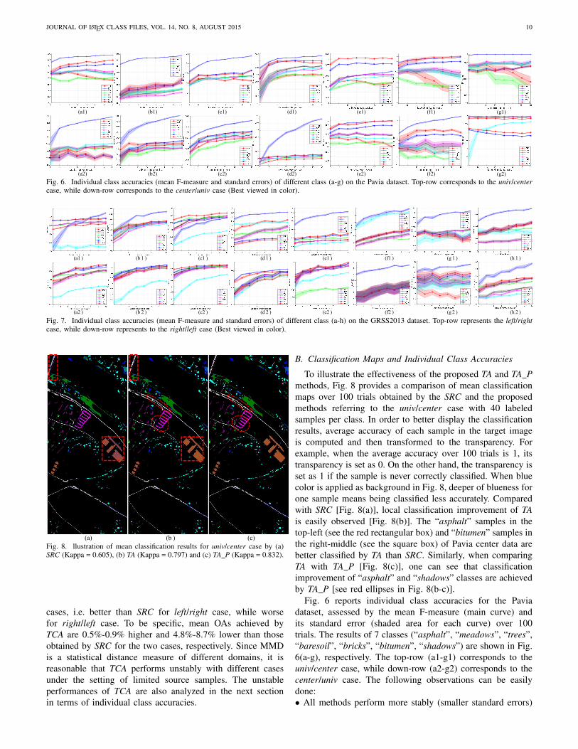
Fig. 6. Individual class accuracies (mean F-measure and standard errors) of different class (a-g) on the Pavia dataset. Top-row corresponds to the univ/centercase, while down-row corresponds to the center/univ case (Best viewed in color).

(a1) (b1) (c1) (d1) (e1) (f1) (g1) (h1)

(a2) (b2) (c2) (d2) (e2) (f2) (g2) (h2)

Fig. 7. Individual class accuracies (mean F-measure and standard errors) of different class (a-h) on the GRSS2013 dataset. Top-row represents the left/rightcase, while down-row represents to the right/left case (Best viewed in color).

(a) (b) (c)Fig. 8. llustration of mean classification results for univ/center case by (a)SRC (Kappa = 0.605), (b) TA (Kappa = 0.797) and (c) TA P (Kappa = 0.832).

cases, i.e. better than SRC for left/right case, while worsefor right/left case. To be specific, mean OAs achieved byTCA are 0.5%-0.9% higher and 4.8%-8.7% lower than thoseobtained by SRC for the two cases, respectively. Since MMDis a statistical distance measure of different domains, it isreasonable that TCA performs unstably with different casesunder the setting of limited source samples. The unstableperformances of TCA are also analyzed in the next sectionin terms of individual class accuracies.

B. Classification Maps and Individual Class Accuracies

To illustrate the effectiveness of the proposed TA and TA Pmethods, Fig. 8 provides a comparison of mean classificationmaps over 100 trials obtained by the SRC and the proposedmethods referring to the univ/center case with 40 labeledsamples per class. In order to better display the classificationresults, average accuracy of each sample in the target imageis computed and then transformed to the transparency. Forexample, when the average accuracy over 100 trials is 1, itstransparency is set as 0. On the other hand, the transparency isset as 1 if the sample is never correctly classified. When bluecolor is applied as background in Fig. 8, deeper of blueness forone sample means being classified less accurately. Comparedwith SRC [Fig. 8(a)], local classification improvement of TAis easily observed [Fig. 8(b)]. The “asphalt” samples in thetop-left (see the red rectangular box) and “bitumen” samples inthe right-middle (see the square box) of Pavia center data arebetter classified by TA than SRC. Similarly, when comparingTA with TA P [Fig. 8(c)], one can see that classificationimprovement of “asphalt” and “shadows” classes are achievedby TA P [see red ellipses in Fig. 8(b-c)].

Fig. 6 reports individual class accuracies for the Paviadataset, assessed by the mean F-measure (main curve) andits standard error (shaded area for each curve) over 100trials. The results of 7 classes (“asphalt”, “meadows”, “trees”,“baresoil”, “bricks”, “bitumen”, “shadows”) are shown in Fig.6(a-g), respectively. The top-row (a1-g1) corresponds to theuniv/center case, while down-row (a2-g2) corresponds to thecenter/univ case. The following observations can be easilydone:• All methods perform more stably (smaller standard errors)


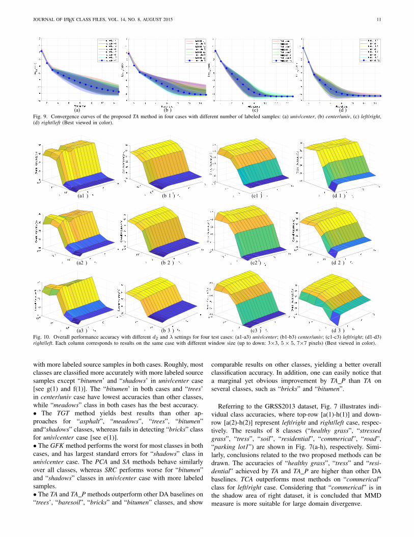
(a) (b) (c) (d)Fig. 9. Convergence curves of the proposed TA method in four cases with different number of labeled samples: (a) univ/center, (b) center/univ, (c) left/right,(d) right/left (Best viewed in color).

(a1) (b1) (c1) (d1)

(a2) (b2) (c2) (d2)

(a3) (b3) (c3) (d3)Fig. 10. Overall performance accuracy with different d2 and λ settings for four test cases: (a1-a3) univ/center; (b1-b3) center/univ; (c1-c3) left/right; (d1-d3)right/left. Each column corresponds to results on the same case with different window size (up to down: 3×3, 5× 5, 7×7 pixels) (Best viewed in color).

with more labeled source samples in both cases. Roughly, mostclasses are classified more accurately with more labeled sourcesamples except “bitumen’ and “shadows’ in univ/center case[see g(1) and f(1)]. The “bitumen’ in both cases and “trees’in center/univ case have lowest accuracies than other classes,while “meadows” class in both cases has the best accuracy.• The TGT method yields best results than other ap-proaches for “asphalt”, “meadows”, “trees”, “bitumen”and“shadows” classes, whereas fails in detecting “bricks” classfor univ/center case [see e(1)].• The GFK method performs the worst for most classes in bothcases, and has largest standard errors for “shadows” class inuniv/center case. The PCA and SA methods behave similarlyover all classes, whereas SRC performs worse for “bitumen”and “shadows” classes in univ/center case with more labeledsamples.• The TA and TA P methods outperform other DA baselines on“trees’, “baresoil”, “bricks” and “bitumen” classes, and show

comparable results on other classes, yielding a better overallclassification accuracy. In addition, one can easily notice thata marginal yet obvious improvement by TA P than TA onseveral classes, such as “bricks” and “bitumen”.

Referring to the GRSS2013 dataset, Fig. 7 illustrates indi-vidual class accuracies, where top-row [a(1)-h(1)] and down-row [a(2)-h(2)] represent left/right and right/left case, respec-tively. The results of 8 classes (“healthy grass”, “stressedgrass”, “tress”, “soil”, “residential”, “commerical”, “road”,“parking lot1”) are shown in Fig. 7(a-h), respectively. Simi-larly, conclusions related to the two proposed methods can bedrawn. The accuracies of “healthy grass”, “tress” and “resi-dential” achieved by TA and TA P are higher than other DAbaselines. TCA outperforms most methods on “commerical”class for left/right case. Considering that “commerical” is inthe shadow area of right dataset, it is concluded that MMDmeasure is more suitable for large domain divergenve.


C. Convergence

We have proved that the TA method is convergent underthe iteratively updating rules of projection matrices and coretensors. Here, we investigate and demonstrate the speed ofthe convergence based on experimental results. Fig. 9 showsthe mean reducing rate of the objective function of TA onthe four test cases over 100 trials (shaded areas representstandard errors). One can see that the objective function valuedecreases by increasing the number of iterations. Moreover,we can observe that the TA converges very fast, usually takingless than 15 iterations. The reducing rate reaches 10e-6 and10e-7 for the Pavia and the GRSS2013 datasets over all the100 trials at the 15-th iteration, respectively. For our MATLABimplementation, 15 iterations take ∼3.3s for univ/center caseswhen 40 labeled samples per class are used.

D. Parameter Sensitivity Analysis

Herein we perform experiments to discuss effects of param-eters of the TA methods in the four cases. For simple and validquantitative analysis, we only employ mean OAs to evaluatedifferent parameter configurations. In detail, window size,spectral dimensionality of TA d2 and manifold regularization λare discussed to achieve better understanding of the proposedmethod. Assuming that the window size is W × W pixels,we set tensor dimensions for MPCA and TA as W ×W × 20and 1× 1× d2, respectively. Note that the number of labeledsamples are fixed to 40 per class for Pavia dataset and 10per class for GRSS2013 dataset, and 10 trials are conductedfor each sub-experiment. Fig. 10 illustrates the mean OAs withrespect to different parameter configurations for the four cases.Each column indicates results using different window sizes foreach case. One can observe that the trends of the mean OAsfor all test cases under different window sizes are nearly thesame, i.e. large value of λ and low value of d2 can both yieldworse accuracy. The observation points out two conclusions: 1)large values of λ force strong geometry preservation, hinderingthe learning of projection matrices; 2) If d2 is smaller than5 for all cases, no enough spectral information is preservedfor training the classifier. However, when d2 is lager than 10,there is no improvement of classification results. To sum up,λ ∈ [0, 0.001] and d2 ∈ [10, 20] can be optimal parametervalues for all cases.

VII. CONCLUSION

This paper has addressed the issue of DA in the classifica-tion of HSI under the assumption of small number of labeledsamples. The main contributions of this paper are the proposedtensor alignment based domain adaptation algorithm and thestrategy based on pure samples extraction for performanceimprovement.

The proposed TA naturally treats each sample in HSI asa 3-D tensor, exploiting the multilinear relationship betweenspatial and spectral dimensions. The shift between 3-D tensorsfrom different domains is reduced by introducing a commonset of projection matrices in the Tucker decomposition. TheTA method mainly contains three steps, i.e. tensors construc-tion, dimension reduction and tensor alignment. Firstly, HSIs

in both domains are segmented into superpixels and eachtensor is constructed by including samples from the samesuperpixel. In this way, the tensors are expected to containsamples belonging to the same class. Then, in order to reducecomputational cost, MPCA is employed for spectral dimensionreduction. In the stage of tensor alignment, to preserve thegeometry of original tensors, two laplacian matrices from bothdomains are first computed. The problem of tensor alignmentis formulated as jointly Tucker decomposition of tensors fromboth domains with manifold regularization on core tensors andorthogonal regularization on projection matrices. The solutionis found by the developed efficient iterative algorithm andthe convergence is analyzed. Once the projection matrices arecomputed, source and target tensors are represented as coretensors. The predicted map of target HSI can be easily obtainedby a supervised classifier.

To further exploit the spatial consistency of HSI, a strategyfor pure samples extraction for performance improvement isthen proposed. The pure samples in each superpixel havesimilar spectral features and likely belong to the same class.Given that samples in one superpixel may belong to twoor even more classes, pure samples may include samplesbelonging to different classes if we increase the number ofpure samples extraction. To extract an appropriate number ofpure samples, we fix the ratio of pure samples (predicted asthe same class) as a constant value. We consider that it isreasonable to assume 70% pure samples in one superpixel.Although the strategy is simple, it turns out to be effective inperformance improvement.

The experiments are conducted on four real HSIs, i.e. PaviaUniversity and City Center, GRSS left and right images. Toexplore the adaptation capacity of TA, different numbers ofsource samples are randomly selected as labeled. Given thecomputational cost of TA, 100 tensors per class from targetdomain are selected for alignment. The TA method yieldsbetter results on univ/center, center/univ and right/left datasets than the other considered DA methods, whereas TCAoutperforms TA on left/right data set. It is found that TCAperforms better than all subspace learning method on the“Commercial” class in the left/right data set. Since the MMD-based TCA method can directly reduce the domain divergence,the “Commercial” class obtained under different conditions inthe left/right data set (non-shadow and shadow area in the twoimages) is better adapted by TCA than by other consideredDA methods. To summarize, the proposed TA method canachieve better performance compared with the state-of-the-artsubspace learning methods when a limited amount of sourcelabeled samples are available.

As future development, the proposed TA method can beeasily extended to manifold regularization orthogonal Tuckerdecomposition for tensor data dimension reduction. Its typicalapplications include multichannel electroencephalographies,multiview images and videos processing.

ACKNOWLEDGMENT

The authors would like to thank Prof. P. Gamba from theUniversity of Pavia for providing the ROSIS data, thank the


Hyperspectral Image Analysis Group and the NSF FundedCenter for Airborne Laser Mapping (NCALM) at the Uni-versity of Houston for providing the grss dfc 2013 data set,and the IEEE GRSS Data Fusion Technical Committee fororganizing the 2013 Data Fusion Contest.

APPENDIX APROOF OF SOLVING EQ. (15)

Theorem 1 Let ΛDVT be the singular value decom-position of ABT, where A ∈ Rm×n and B ∈ Rp×n.Then X = ΛIm×pVT is an orthogonal matric minimizing||A−XB||2F, where Im×p is a matrix with diagonal elementsall are 1 while others are 0.Proof. To derive the method we first expand ||A−XB||2F:

||A−XB||2F = ||A||2F + ||B||2F − 2tr(XTABT) (18)

So picking X to maximize tr(XTABT) will minimize ||A−XB||2F. Let ΛDVT be the singular value decomposition ofABT. Then we have:

tr(XTABT) = tr(XTΛDVT) = tr(VTXTΛD) (19)

Write Z = VTXTΛ, notice Z is orthogonal (being the productof orthogonal matrices). The goal is re-stated: maximizetr(ZD) through our choice of X. Since D is diagonal, thentr(ZD) =

∑i ZiiDii. The Dii are non-negative and Z is

orthogonal for any choice of X. The maximum is achieved bychoosing X such that all of Zii = 1 which implies Z = Im×p.So an optimal X is ΛIm×pVT.

REFERENCES

[1] M. Fauvel, Y. Tarabalka, J. A. Benediktsson, J. Chanussot, and J. C.Tilton, “Advances in spectral-spatial classification of hyperspectral im-ages,” Proceedings of the IEEE, vol. 101, no. 3, pp. 652–675, 2013.

[2] G. Camps-Valls, D. Tuia, L. Bruzzone, and J. A. Benediktsson, “Ad-vances in hyperspectral image classification: Earth monitoring withstatistical learning methods,” IEEE signal processing magazine, vol. 31,no. 1, pp. 45–54, 2014.

[3] D. Tuia, C. Persello, and L. Bruzzone, “Domain adaptation for theclassification of remote sensing data: An overview of recent advances,”IEEE geoscience and remote sensing magazine, vol. 4, no. 2, pp. 41–57,2016.

[4] S. Schneider, R. J. Murphy, and A. Melkumyan, “Evaluating theperformance of a new classifier–the gp-oad: A comparison with existingmethods for classifying rock type and mineralogy from hyperspectralimagery,” ISPRS Journal of Photogrammetry and Remote Sensing,vol. 98, pp. 145–156, 2014.

[5] K. Tiwari, M. Arora, and D. Singh, “An assessment of independentcomponent analysis for detection of military targets from hyperspec-tral images,” International Journal of Applied Earth Observation andGeoinformation, vol. 13, no. 5, pp. 730–740, 2011.

[6] J. Ham, Y. Chen, M. M. Crawford, and J. Ghosh, “Investigation of therandom forest framework for classification of hyperspectral data,” IEEETransactions on Geoscience and Remote Sensing, vol. 43, no. 3, pp.492–501, 2005.

[7] F. Melgani and L. Bruzzone, “Classification of hyperspectral remotesensing images with support vector machines,” IEEE Transactions ongeoscience and remote sensing, vol. 42, no. 8, pp. 1778–1790, 2004.

[8] M. Belkin, P. Niyogi, and V. Sindhwani, “Manifold regularization: Ageometric framework for learning from labeled and unlabeled examples,”Journal of machine learning research, vol. 7, no. Nov, pp. 2399–2434,2006.

[9] S. Melacci and M. Belkin, “Laplacian support vector machines trainedin the primal,” Journal of Machine Learning Research, vol. 12, no. Mar,pp. 1149–1184, 2011.

[10] W. Yang, X. Yin, and G.-S. Xia, “Learning high-level features forsatellite image classification with limited labeled samples,” IEEE Trans-actions on Geoscience and Remote Sensing, vol. 53, no. 8, pp. 4472–4482, 2015.

[11] S. Delalieux, B. Somers, B. Haest, T. Spanhove, J. V. Borre, andC. Mucher, “Heathland conservation status mapping through integrationof hyperspectral mixture analysis and decision tree classifiers,” Remotesensing of environment, vol. 126, pp. 222–231, 2012.

[12] X. Guo, X. Huang, L. Zhang, L. Zhang, A. Plaza, and J. A. Benedik-tsson, “Support tensor machines for classification of hyperspectralremote sensing imagery,” IEEE Transactions on Geoscience and RemoteSensing, vol. 54, no. 6, pp. 3248–3264, 2016.

[13] L. Bruzzone and M. Marconcini, “Domain adaptation problems: Adasvm classification technique and a circular validation strategy,” IEEEtransactions on pattern analysis and machine intelligence, vol. 32, no. 5,pp. 770–787, 2010.

[14] V. M. Patel, R. Gopalan, R. Li, and R. Chellappa, “Visual domainadaptation: A survey of recent advances,” IEEE signal processingmagazine, vol. 32, no. 3, pp. 53–69, 2015.

[15] S. J. Pan and Q. Yang, “A survey on transfer learning,” IEEE Trans-actions on knowledge and data engineering, vol. 22, no. 10, pp. 1345–1359, 2010.

[16] M. A. O. Vasilescu and D. Terzopoulos, “Multilinear subspace analysisof image ensembles,” in Computer Vision and Pattern Recognition, 2003.Proceedings. 2003 IEEE Computer Society Conference on, vol. 2. IEEE,2003, pp. II–93.

[17] H. Lu, L. Zhang, Z. Cao, W. Wei, K. Xian, C. Shen, and A. van denHengel, “When unsupervised domain adaptation meets tensor represen-tations,” in The IEEE International Conference on Computer Vision(ICCV), vol. 2, 2017.

[18] Z. Zhong, B. Fan, J. Duan, L. Wang, K. Ding, S. Xiang, and C. Pan,“Discriminant tensor spectral–spatial feature extraction for hyperspectralimage classification,” IEEE Geoscience and Remote Sensing Letters,vol. 12, no. 5, pp. 1028–1032, 2015.

[19] L. Zhang, L. Zhang, D. Tao, X. Huang, and B. Du, “Compression ofhyperspectral remote sensing images by tensor approach,” Neurocom-puting, vol. 147, pp. 358–363, 2015.

[20] Y. Xu, X. Fang, J. Wu, X. Li, and D. Zhang, “Discriminative transfersubspace learning via low-rank and sparse representation,” IEEE Trans-actions on Image Processing, vol. 25, no. 2, pp. 850–863, 2016.

[21] Z. Feng, M. Wang, S. Yang, Z. Liu, L. Liu, B. Wu, and H. Li,“Superpixel tensor sparse coding for structural hyperspectral imageclassification,” IEEE Journal of Selected Topics in Applied Earth Ob-servations and Remote Sensing, vol. 10, no. 4, pp. 1632–1639, 2017.

[22] Z. He, J. Hu, and Y. Wang, “Low-rank tensor learning for classificationof hyperspectral image with limited labeled samples,” Signal Processing,vol. 145, pp. 12–25, 2018.

[23] P. Koniusz, Y. Tas, and F. Porikli, “Domain adaptation by mixture ofalignments of second-or higher-order scatter tensors,” in Proc. IEEEConference on Computer Vision and Pattern Recognition (CVPR), vol. 1,2017.

[24] T. G. Kolda and B. W. Bader, “Tensor decompositions and applications,”SIAM review, vol. 51, no. 3, pp. 455–500, 2009.

[25] A. A. Nielsen and M. J. Canty, “Kernel principal component andmaximum autocorrelation factor analyses for change detection,” in Imageand signal processing for remote sensing XV, vol. 7477. InternationalSociety for Optics and Photonics, 2009, p. 74770T.

[26] B. Fernando, A. Habrard, M. Sebban, and T. Tuytelaars, “Unsupervisedvisual domain adaptation using subspace alignment,” in Computer Vision(ICCV), 2013 IEEE International Conference on. IEEE, 2013, pp.2960–2967.

[27] A. A. Nielsen, “The regularized iteratively reweighted mad method forchange detection in multi-and hyperspectral data,” IEEE Transactionson Image processing, vol. 16, no. 2, pp. 463–478, 2007.

[28] M. Volpi, G. Camps-Valls, and D. Tuia, “Spectral alignment of multi-temporal cross-sensor images with automated kernel canonical correla-tion analysis,” ISPRS Journal of Photogrammetry and Remote Sensing,vol. 107, pp. 50–63, 2015.

[29] A. Samat, C. Persello, P. Gamba, S. Liu, J. Abuduwaili, and E. Li, “Su-pervised and semi-supervised multi-view canonical correlation analysisensemble for heterogeneous domain adaptation in remote sensing imageclassification,” Remote sensing, vol. 9, no. 4, p. 337, 2017.

[30] R. Gopalan, R. Li, and R. Chellappa, “Domain adaptation for objectrecognition: An unsupervised approach,” in Computer Vision (ICCV),2011 IEEE International Conference on. IEEE, 2011, pp. 999–1006.

[31] B. Gong, Y. Shi, F. Sha, and K. Grauman, “Geodesic flow kernelfor unsupervised domain adaptation,” in Computer Vision and Pattern


Recognition (CVPR), 2012 IEEE Conference on. IEEE, 2012, pp. 2066–2073.

[32] A. Samat, P. Gamba, J. Abuduwaili, S. Liu, and Z. Miao, “Geodesic flowkernel support vector machine for hyperspectral image classification byunsupervised subspace feature transfer,” Remote Sensing, vol. 8, no. 3,p. 234, 2016.

[33] B. Banerjee and S. Chaudhuri, “Hierarchical subspace learning basedunsupervised domain adaptation for cross-domain classification of re-mote sensing images,” IEEE Journal of Selected Topics in Applied EarthObservations and Remote Sensing, vol. 10, no. 11, pp. 5099–5109, 2017.

[34] B. Banerjee and K. M. Buddhiraju, “Domain adaptation in the absenceof source domain labeled samplesa coclustering-based approach,” IEEEGeoscience and Remote Sensing Letters, vol. 13, no. 12, pp. 1905–1909,2016.

[35] I.-H. Jhuo, D. Liu, D. Lee, and S.-F. Chang, “Robust visual domainadaptation with low-rank reconstruction,” in Computer Vision and Pat-tern Recognition (CVPR), 2012 IEEE Conference on. IEEE, 2012, pp.2168–2175.

[36] M. Shao, D. Kit, and Y. Fu, “Generalized transfer subspace learningthrough low-rank constraint,” International Journal of Computer Vision,vol. 109, no. 1-2, pp. 74–93, 2014.

[37] Y. Xu, X. Fang, J. Wu, X. Li, and D. Zhang, “Discriminative transfersubspace learning via low-rank and sparse representation,” IEEE Trans-actions on Image Processing, vol. 25, no. 2, pp. 850–863, 2016.

[38] J. Li, Y. Wu, and K. Lu, “Structured domain adaptation,” IEEE Trans-actions on Circuits and Systems for Video Technology, vol. 27, no. 8,pp. 1700–1713, 2017.

[39] L. Zhang, W. Zuo, and D. Zhang, “Lsdt: Latent sparse domain transferlearning for visual adaptation,” IEEE Transactions on Image Processing,vol. 25, no. 3, pp. 1177–1191, 2016.

[40] Q. Shi, B. Du, and L. Zhang, “Domain adaptation for remote sensingimage classification: A low-rank reconstruction and instance weightinglabel propagation inspired algorithm,” IEEE Transactions on Geoscienceand Remote Sensing, vol. 53, no. 10, pp. 5677–5689, 2015.

[41] S. J. Pan, I. W. Tsang, J. T. Kwok, and Q. Yang, “Domain adaptation viatransfer component analysis,” IEEE Transactions on Neural Networks,vol. 22, no. 2, pp. 199–210, 2011.

[42] G. Matasci, M. Volpi, M. Kanevski, L. Bruzzone, and D. Tuia, “Semisu-pervised transfer component analysis for domain adaptation in remotesensing image classification,” IEEE Transactions on Geoscience andRemote Sensing, vol. 53, no. 7, pp. 3550–3564, 2015.

[43] M. Long, J. Wang, G. Ding, J. Sun, and S. Y. Philip, “Transfer featurelearning with joint distribution adaptation,” in Computer Vision (ICCV),2013 IEEE International Conference on. IEEE, 2013, pp. 2200–2207.

[44] M. Long, J. Wang, G. Ding, J. Sun, and P. S. Yu, “Transfer jointmatching for unsupervised domain adaptation,” in Proceedings of theIEEE conference on computer vision and pattern recognition, 2014, pp.1410–1417.

[45] J. Zhang, W. Li, and P. Ogunbona, “Joint geometrical and sta-tistical alignment for visual domain adaptation,” arXiv preprintarXiv:1705.05498, 2017.

[46] H. Sun, S. Liu, S. Zhou, and H. Zou, “Transfer sparse subspace analysisfor unsupervised cross-view scene model adaptation,” IEEE Journal ofSelected Topics in Applied Earth Observations and Remote Sensing,vol. 9, no. 7, pp. 2901–2909, 2016.

[47] ——, “Unsupervised cross-view semantic transfer for remote sensingimage classification,” IEEE Geoscience and Remote Sensing Letters,vol. 13, no. 1, pp. 13–17, 2016.

[48] D. Tuia, M. Volpi, M. Trolliet, and G. Camps-Valls, “Semisupervisedmanifold alignment of multimodal remote sensing images,” IEEE Trans-actions on Geoscience and Remote Sensing, vol. 52, no. 12, pp. 7708–7720, 2014.

[49] D. Tuia and G. Camps-Valls, “Kernel manifold alignment for domainadaptation,” PloS one, vol. 11, no. 2, p. e0148655, 2016.

[50] H. L. Yang and M. M. Crawford, “Spectral and spatial proximity-basedmanifold alignment for multitemporal hyperspectral image classifica-tion,” IEEE Transactions on Geoscience and Remote Sensing, vol. 54,no. 1, pp. 51–64, 2016.

[51] ——, “Domain adaptation with preservation of manifold geometry forhyperspectral image classification,” IEEE Journal of Selected Topics inApplied Earth Observations and Remote Sensing, vol. 9, no. 2, pp. 543–555, 2016.

[52] C. Luo and L. Ma, “Manifold regularized distribution adaptation forclassification of remote sensing images,” IEEE Access, 2018.

[53] L. Zhu and L. Ma, “Class centroid alignment based domain adaptationfor classification of remote sensing images,” Pattern Recognition Letters,vol. 83, pp. 124–132, 2016.

[54] S. Inamdar, F. Bovolo, L. Bruzzone, and S. Chaudhuri, “Multidimen-sional probability density function matching for preprocessing of mul-titemporal remote sensing images,” IEEE Transactions on Geoscienceand Remote Sensing, vol. 46, no. 4, pp. 1243–1252, 2008.

[55] D. Tuia, J. Munoz-Mari, L. Gomez-Chova, and J. Malo, “Graph match-ing for adaptation in remote sensing,” IEEE Transactions on Geoscienceand Remote Sensing, vol. 51, no. 1, pp. 329–341, 2013.

[56] Y. Qian, M. Ye, and J. Zhou, “Hyperspectral image classification basedon structured sparse logistic regression and three-dimensional wavelettexture features,” IEEE Transactions on Geoscience and Remote Sensing,vol. 51, no. 4, pp. 2276–2291, 2013.

[57] F. Tsai and J.-S. Lai, “Feature extraction of hyperspectral image cubesusing three-dimensional gray-level cooccurrence,” IEEE transactions ongeoscience and remote sensing, vol. 51, no. 6, pp. 3504–3513, 2013.

[58] L. Zhang, L. Zhang, D. Tao, and X. Huang, “Tensor discrimina-tive locality alignment for hyperspectral image spectral–spatial featureextraction,” IEEE Transactions on Geoscience and Remote Sensing,vol. 51, no. 1, pp. 242–256, 2013.

[59] Z. Zhong, B. Fan, J. Duan, L. Wang, K. Ding, S. Xiang, and C. Pan,“Discriminant tensor spectral–spatial feature extraction for hyperspectralimage classification,” IEEE Geoscience and Remote Sensing Letters,vol. 12, no. 5, pp. 1028–1032, 2015.

[60] Z. Feng, M. Wang, S. Yang, Z. Liu, L. Liu, B. Wu, and H. Li,“Superpixel tensor sparse coding for structural hyperspectral imageclassification,” IEEE Journal of Selected Topics in Applied Earth Ob-servations and Remote Sensing, vol. 10, no. 4, pp. 1632–1639, 2017.

[61] Z. He, J. Li, L. Liu, and Y. Shen, “Three-dimensional empirical modedecomposition (temd): A fast approach motivated by separable filters,”Signal Processing, vol. 131, pp. 307–319, 2017.

[62] Z. He, J. Li, L. Liu, K. Liu, and L. Zhuo, “Fast three-dimensional em-pirical mode decomposition of hyperspectral images for class-orientedmultitask learning,” IEEE Transactions on Geoscience and RemoteSensing, vol. 54, no. 11, pp. 6625–6643, 2016.

[63] Y.-J. Deng, H.-C. Li, L. Pan, L.-Y. Shao, Q. Du, and W. J. Emery, “Mod-ified tensor locality preserving projection for dimensionality reductionof hyperspectral images,” IEEE Geoscience and Remote Sensing Letters,2018.

[64] R. Achanta, A. Shaji, K. Smith, A. Lucchi, P. Fua, and S. Susstrunk,“Slic superpixels compared to state-of-the-art superpixel methods,” IEEEtransactions on pattern analysis and machine intelligence, vol. 34,no. 11, pp. 2274–2282, 2012.

[65] G. Martin and A. Plaza, “Spatial-spectral preprocessing prior to end-member identification and unmixing of remotely sensed hyperspectraldata,” IEEE journal of selected topics in applied earth observations andremote sensing, vol. 5, no. 2, pp. 380–395, 2012.

Yao Qin (SM’ 16) received the B.S degree inInformation Engineering from Shanghai JiaotongUniversity, Shanghai, China, in 2013 and the M. S.degree from School of Electronic and Engineering,National University of Defence Technology, Chang-sha, China, in 2015. Currently, he is pursuing thePh. D. degree and is a visiting Ph. D at RSLabin the Department of Information Engineering andComputer Science, University of Trento, Italy. Hismajor research interests are remote sensing imageclassification and domain adaptation.


Lorenzo Bruzzone (S’95-M’98-SM’03-F’10) re-ceived the Laurea (M.S.) degree in electronic engi-neering (summa cum laude) and the Ph.D. degree intelecommunications from the University of Genoa,Italy, in 1993 and 1998, respectively.

He is currently a Full Professor of telecommuni-cations at the University of Trento, Italy, where heteaches remote sensing, radar, and digital communi-cations. Dr. Bruzzone is the founder and the directorof the Remote Sensing Laboratory in the Departmentof Information Engineering and Computer Science,

University of Trento. His current research interests are in the areas of remotesensing, radar and SAR, signal processing, machine learning and patternrecognition. He promotes and supervises research on these topics within theframeworks of many national and international projects. He is the PrincipalInvestigator of many research projects. Among the others, he is the PrincipalInvestigator of the Radar for icy Moon exploration (RIME) instrument inthe framework of the JUpiter ICy moons Explorer (JUICE) mission of theEuropean Space Agency. He is the author (or coauthor) of 215 scientificpublications in referred international journals (154 in IEEE journals), morethan 290 papers in conference proceedings, and 21 book chapters. He iseditor/co-editor of 18 books/conference proceedings and 1 scientific book. Hispapers are highly cited, as proven form the total number of citations (morethan 25000) and the value of the h-index (74) (source: Google Scholar). Hewas invited as keynote speaker in more than 30 international conferences andworkshops. Since 2009 he is a member of the Administrative Committee ofthe IEEE Geoscience and Remote Sensing Society (GRSS).

Dr. Bruzzone ranked first place in the Student Prize Paper Competitionof the 1998 IEEE International Geoscience and Remote Sensing Symposium(IGARSS), Seattle, July 1998. Since that he was recipient of many interna-tional and national honors and awards, including the recent IEEE GRSS 2015Outstanding Service Award and the 2017 IEEE IGARSS Symposium PrizePaper Award. Dr. Bruzzone was a Guest Co-Editor of many Special Issues ofinternational journals. He is the co-founder of the IEEE International Work-shop on the Analysis of Multi-Temporal Remote-Sensing Images (MultiTemp)series and is currently a member of the Permanent Steering Committee of thisseries of workshops. Since 2003 he has been the Chair of the SPIE Conferenceon Image and Signal Processing for Remote Sensing. He has been the founderof the IEEE Geoscience and Remote Sensing Magazine for which he hasbeen Editor-in-Chief between 2013-2017.Currently he is an Associate Editorfor the IEEE Transactions on Geoscience and Remote Sensing. He has beenDistinguished Speaker of the IEEE Geoscience and Remote Sensing Societybetween 2012-2016.

Biao Li was born in Zhejiang, China, in 1968. He received the Ph.D.degrees in the School of Electronic Science, National University of DefenseTechnology, Changsha, China, in 1998, where he is currently a full professor.His current research interests include signal processing and infrared imageprocessing.

Tensor Alignment Based Domain Adaptation for Hyperspectral ...

Documents

Transcript of Tensor Alignment Based Domain Adaptation for Hyperspectral ...