remote sensing

Letter

Comparison of Hyperspectral Versus Traditional FieldMeasurements of Fractional Ground Cover in theAustralian Arid Zone

Claire Fisk * , Kenneth D. Clarke and Megan M. Lewis

School of Biological Sciences, The University of Adelaide, Adelaide 5005, Australia;kenneth.clarke@adelaide.edu.au (K.D.C.); megan.lewis@adelaide.edu.au (M.M.L.)* Correspondence: claire.fisk@adelaide.edu.au

Received: 1 October 2019; Accepted: 26 November 2019; Published: 28 November 2019�����������������

Abstract: The collection of high-quality field measurements of ground cover is critical for calibrationand validation of fractional ground cover maps derived from satellite imagery. Field-basedhyperspectral ground cover sampling is a potential alternative to traditional in situ techniques.This study aimed to develop an effective sampling design for spectral ground cover surveys in orderto estimate fractional ground cover in the Australian arid zone. To meet this aim, we addressedtwo key objectives: (1) Determining how spectral surveys and traditional step-point samplingcompare when conducted at the same spatial scale and (2) comparing these two methods to currentAustralian satellite-derived fractional cover products. Across seven arid, sparsely vegetated surveysites, six 500-m transects were established. Ground cover reflectance was recorded taking continuoushyperspectral readings along each transect while step-point surveys were conducted along thesame transects. Both measures of ground cover were converted into proportions of photosyntheticvegetation, non-photosynthetic vegetation, and bare soil for each site. Comparisons were made ofthe proportions of photosynthetic vegetation, non-photosynthetic vegetation, and bare soil derivedfrom both in situ methods as well as MODIS and Landsat fractional cover products. We foundstrong correlations between fractional cover derived from hyperspectral and step-point samplingconducted at the same spatial scale at our survey sites. Comparison of the in situ measurementsand image-derived fractional cover products showed that overall, the Landsat product was stronglyrelated to both in situ methods for non-photosynthetic vegetation and bare soil whereas the MODISproduct was strongly correlated with both in situ methods for photosynthetic vegetation. This studydemonstrates the potential of the spectral transect method, both in its ability to produce resultscomparable to the traditional transect measures, but also in its improved objectivity and relativelogistic ease. Future efforts should be made to include spectral ground cover sampling as part ofAustralia’s plan to produce calibration and validation datasets for remotely sensed products.

Keywords: calibration; ground cover; hyperspectral; spectral unmixing; validation

1. Introduction

Satellite image-derived fractional ground cover mapping has proven to be an essential sourceof information for applications, including analysis of spatial and temporal vegetation dynamics [1],monitoring urban greenness [2], mapping bushfire burn severity levels [3], forest cover change [4], anddeforestation [5]. Algorithms, including spectral mixture analysis [6–8], multiple endmember spectralmixture analysis [9], and relative spectral mixture analysis [10], are used to produce fractional cover(FC) maps. These algorithms can be applied to multispectral and hyperspectral imagery, decomposingeach image pixel into a measure of similarity to two or more spectrally distinct land cover types. These

Remote Sens. 2019, 11, 2825; doi:10.3390/rs11232825 www.mdpi.com/journal/remotesensing

Remote Sens. 2019, 11, 2825 2 of 13

typically include photosynthetic vegetation (PV), non-photosynthetic vegetation (NPV), bare soil (BS),shadow, and snow [6,10], with the resulting maps providing quantitative estimates of the proportionof the cover types comprising each pixel.

Fractional cover mapping has been performed across a range of scales, including global mappingprojects as such the Copernicus Global Land Service, which has produced a 300-m and a 1-km fractionof green vegetation cover product based on PROBA-V and SPOT-VGT imagery [11,12]. Local studieshave used FC products to assist water quality management of catchments [13], urban land covermapping [14], and the study of savanna vegetation morphology [15,16]. In Australia, time series offractional cover have been produced from MODIS [17] and Landsat [18,19] and are being used widelyfor environmental assessment and monitoring applications.

Calibration and validation are essential for ensuring the reliability and consistency of FC products.Data used for calibration and validation of fractional cover are derived from a variety of sources andtechniques, and there is currently no international standard. Lawley et al. [20], Montesano et al. [21],Morisette et al. [22], and Xiao and Moody [23] all utilised remotely sensed imagery with high spatialresolution to validate FC products with lower spatial resolution. The advantages of this approach arethat high-spatial resolution imagery provides an objective record at the time of the region being assessedand may allow for the validation of areas that cannot be easily accessed. Alternative evaluationshave sought to avoid subjective on-ground assessments of ground cover and instead have used acombination of qualitative and quantitative data for assessment. For example, Guerschman et al. [16]utilised two qualitative datasets to calibrate the Australian MODIS fractional cover product: (1) Ageneral description of vegetation type and condition, including photographs of each site, and (2) avectorized fire scar map that classified areas of the landscape as either burnt or unburnt.

Common approaches to in situ measurement of ground cover, demonstrated by Scarth, Röder, andDenham [24], Asner and Heidebrecht [25], and Lewis [26], have utilised variants of point-based samplingtechniques that were initially developed for vegetation ecology and rangeland assessment [27–29].These methods include line-point intercept transects, step-point surveys, and wheel-point surveys,where observers walk across a study area making point-based observations at defined intervals. Acrossa survey area, hundreds of point-based observations are used to estimate FC. Point observationsgenerally categorise ground cover into defined classes, such as rock, disturbed soil, green leaf, anddry leaf, which are later aggregated into broader classes, such as PV, NPV, and BS, matching the fieldclasses with the image product being assessed. Muir et al. [30] developed an Australian nationalstandard for field measurements of fractional ground cover, which provides a well-documented, easilyrepeatable method that is now widely used.

Although field protocols have been developed to improve consistency and reduce the potential forerrors, subjective human judgements are still required, and these may affect the data significantly [31].In such surveys, observers are required to make hundreds of rapid decisions, only having a fewseconds to observe and record the cover type before moving on. Most cover types are relativelyeasy to discriminate in the field but distinguishing between PV and NPV can be a difficult task. PVand NPV are better thought of as extremes of a continuum, rather than binary categories, and hencedistinguishing between PV and NPV can be difficult for observers [32].

A technique that has the potential to help reduce subjectivity is to estimate the relative fractions ofPV, NPV, and BS from field-based hyperspectral reflectance measurements. While in situ hyperspectralmeasurements have been used for radiometric and spectral calibration and validation of remotelysensed products [33,34], and may provide reference signatures for image analyses [17,18], they have notbeen used explicitly for the validation of fractional ground cover products until Meyer and Okin [35].This method records many in situ spectra over a study area, which in their aggregate, capture thecombined spectral response of the site. The relative proportions of PV, NPV, and BS can then be unmixedfrom the field spectra. Using this approach Meyer and Okin [35] demonstrated a stronger agreementbetween FC values derived from field-based reflectance measurements and their image-based productthan between traditional line-point intercept observations and their image-based product, which

Remote Sens. 2019, 11, 2825 3 of 13

showed low correlations. In our paper, hyperspectral ground surveys refer to the collection of spectralmeasurements over an area for the purpose of estimating ground cover fractions [33], quite a differentapplication to the use of in situ spectroscopic measurements for radiometric calibration of imagery.

Another challenge for calibration and validation is to match the scale of field data with that ofbroad-scale FC products. When validating products developed from coarse resolution imagery (e.g.,500 m), it is common to up-scale field data recorded at a finer scale (e.g., 100 m) in order to determinethe accuracy of the coarse resolution products. This is usually conducted under the assumption thatthe area around the sample site is homogenous and similar to that surveyed. For example, Meyerand Okin [35] conducted spectral sampling over 500-m transects to correspond to a MODIS pixeland compared the results to line-point intercept sampling that was conducted over smaller 100-mtransects. A potential reason for the low correlation between the sampling methods is that the 100-mtransects were insufficient to gain an adequate estimate of the ground cover for a 500-m pixel. Meyerand Okin [35] were following the Muir et al. [30] field sampling layout, where transects were placedin a radiating star pattern that was designed to relate field measurements to Landsat imagery. TheMuir et al. [30] design samples three 100-m transects, which covers approximately 3 × 3 Landsatpixels, making it ideal for validating Landsat-based products but not necessarily adequate for coarserresolution products (MODIS).

The layout of transects also has the potential to affect how an area is sampled. For instance,the star-transect method includes a sampling bias that over-represents cover towards the centre ofthe plot. Three transects are placed in a star pattern with the result being that observation pointsare concentrated in the centre of the star and increasingly dispersed as the distance from the centreincreases. Therefore, a sampling pattern that provides a more even distribution across a site mayprovide a better representation of the ground cover. Other studies have placed parallel transects evenlyacross sample sites [26,36] or placed transects in a grid pattern in order to more evenly sample thearea [37].

Field-based hyperspectral ground cover sampling is a potential alternative to traditional techniquesthat may assist with the calibration and validation of remotely sensed products. The motivation forthis research is to expand upon the work of Meyer and Okin [35] and trial hyperspectral ground coversampling in Australia, with the ultimate aim of incorporating spectral sampling as part of Australia’snational effort to collect validation and calibration data to meet our remote sensing needs. Our aimwas to develop an effective sampling design for spectral ground cover surveys in order to estimatefractional ground cover. Our objectives were (1) to determine how spectral surveys and traditionalstep-point sampling compare when conducted at the same spatial scale, and (2) determine how thesein situ methods compare to current Australian satellite-derived FC products.

2. Materials and Methods

Currently, in situ validation data collected using the Muir et al. [30] method is used to assess theaccuracy of both the MODIS and Landsat products. Meyer and Okin [35] found that the in situ spectralmeasurements they collected could be used to validate fractional ground cover mapping developedfrom MODIS imagery over Botswana, but this has not been tested across other environments. Tomeet our objectives, we therefore completed ground cover surveys before inspecting how our in situmeasurements would compare with the MODIS and Landsat products. Figure 1 provides an overviewof the methods used in this study.

Remote Sens. 2019, 11, 2825 4 of 13Remote Sens. 2019, 11, x FOR PEER REVIEW 4 of 13

Figure 1. Flowchart outlining the methodological approach taken in this paper.

2.1. Study Area

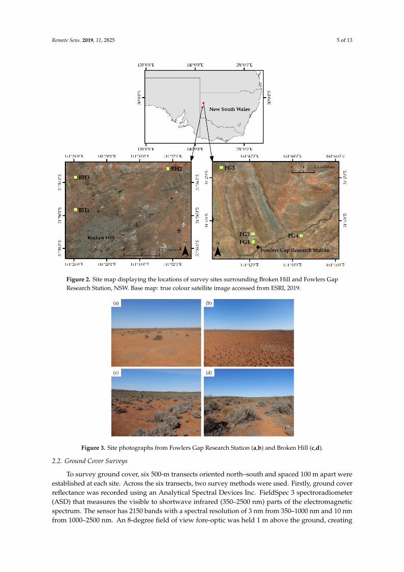
The study was conducted in New South Wales (NSW), Australia within the arid zone (Figure 2). Sites FG1–FG4 (Figure 3a,b) were situated at Fowlers Gap Arid Research Station, 110 km north of Broken Hill, NSW, while sites BH1–BH3 (Figure 3c,d) were located surrounding the City of Broken Hill. The climate for both regions is hot and persistently dry [38]. Fowlers Gap has a mean annual rainfall of 240 mm, a mean annual minimum temperature of 13 ᵒC, and a mean annual maximum temperature of 26.9 ᵒC [39]. The vegetation at Fowlers Gap comprises low open chenopodiaceous shrublands, some low open Acacia and Casuarina woodland as well as grasslands on the plains Mabbutt et al. [40]. Broken Hill has a mean annual rainfall of 250 mm with a mean annual minimum temperature of 11.8 ᵒC and a mean annual maximum temperature of 24.7 ᵒC [41]. The vegetation around Broken Hill is also composed of chenopod shrublands that includes saltbush and bluebush communities as well as Mulga (Acacia aneura) [42].

Figure 1. Flowchart outlining the methodological approach taken in this paper.

2.1. Study Area

The study was conducted in New South Wales (NSW), Australia within the arid zone (Figure 2).Sites FG1–FG4 (Figure 3a,b) were situated at Fowlers Gap Arid Research Station, 110 km north ofBroken Hill, NSW, while sites BH1–BH3 (Figure 3c,d) were located surrounding the City of Broken Hill.The climate for both regions is hot and persistently dry [38]. Fowlers Gap has a mean annual rainfall of240 mm, a mean annual minimum temperature of 13 ◦C, and a mean annual maximum temperature of26.9 ◦C [39]. The vegetation at Fowlers Gap comprises low open chenopodiaceous shrublands, somelow open Acacia and Casuarina woodland as well as grasslands on the plains Mabbutt et al. [40]. BrokenHill has a mean annual rainfall of 250 mm with a mean annual minimum temperature of 11.8 ◦C anda mean annual maximum temperature of 24.7 ◦C [41]. The vegetation around Broken Hill is alsocomposed of chenopod shrublands that includes saltbush and bluebush communities as well as Mulga(Acacia aneura) [42].

Remote Sens. 2019, 11, 2825 5 of 13Remote Sens. 2019, 11, x FOR PEER REVIEW 5 of 13

Figure 2. Site map displaying the locations of survey sites surrounding Broken Hill and Fowlers Gap Research Station, NSW. Base map: true colour satellite image accessed from ESRI, 2019.

Figure 3. Site photographs from Fowlers Gap Research Station (a,b) and Broken Hill (c,d).

2.2. Ground Cover Surveys

To survey ground cover, six 500-m transects oriented north–south and spaced 100 m apart were established at each site. Across the six transects, two survey methods were used. Firstly, ground cover reflectance was recorded using an Analytical Spectral Devices Inc. FieldSpec 3 spectroradiometer (ASD) that measures the visible to shortwave infrared (350–2500 nm) parts of the electromagnetic spectrum. The sensor has 2150 bands with a spectral resolution of 3 nm from 350–1000 nm and 10 nm

Figure 2. Site map displaying the locations of survey sites surrounding Broken Hill and Fowlers GapResearch Station, NSW. Base map: true colour satellite image accessed from ESRI, 2019.

Remote Sens. 2019, 11, x FOR PEER REVIEW 5 of 13

Figure 2. Site map displaying the locations of survey sites surrounding Broken Hill and Fowlers Gap Research Station, NSW. Base map: true colour satellite image accessed from ESRI, 2019.

Figure 3. Site photographs from Fowlers Gap Research Station (a,b) and Broken Hill (c,d).

2.2. Ground Cover Surveys

To survey ground cover, six 500-m transects oriented north–south and spaced 100 m apart were established at each site. Across the six transects, two survey methods were used. Firstly, ground cover reflectance was recorded using an Analytical Spectral Devices Inc. FieldSpec 3 spectroradiometer (ASD) that measures the visible to shortwave infrared (350–2500 nm) parts of the electromagnetic spectrum. The sensor has 2150 bands with a spectral resolution of 3 nm from 350–1000 nm and 10 nm

Figure 3. Site photographs from Fowlers Gap Research Station (a,b) and Broken Hill (c,d).

2.2. Ground Cover Surveys

To survey ground cover, six 500-m transects oriented north–south and spaced 100 m apart wereestablished at each site. Across the six transects, two survey methods were used. Firstly, ground coverreflectance was recorded using an Analytical Spectral Devices Inc. FieldSpec 3 spectroradiometer(ASD) that measures the visible to shortwave infrared (350–2500 nm) parts of the electromagneticspectrum. The sensor has 2150 bands with a spectral resolution of 3 nm from 350–1000 nm and 10 nmfrom 1000–2500 nm. An 8-degree field of view fore-optic was held 1 m above the ground, creating

Remote Sens. 2019, 11, 2825 6 of 13

a 0.14-m diameter ground field of view. At the start of each transect, and as required, the devicewas optimized and white reference measurements taken following the recommended protocols [43].The operator of the ASD walked along each transect at a consistent pace taking continuous readingsof ground cover reflectance. The continuous readings were averaged by the ASD and 10 averagedspectra were recorded for each 25-m segment of the transect, totalling 200 spectra per transect (1200measurements per site).

The second method used was step-point sampling, where an observer collected point-basedobservations of ground cover along the six transects. The observer marked a point on a boot tip and at5-m intervals recorded the cover that intersected the point. Cover was categorised into a set numberof cover types, including crust, rock, litter, green leaf, and dry leaf, as outlined in the Muir et al. [30]protocol. The cover for each of these categories was calculated as the proportion of the total number ofpoint observations at the site (n = 600). These categories were grouped into three broad classes, PV,NPV, and BS, to give their FC percentage within the site.

2.3. Endmember Extraction and Spectral Unmixing

The hyperspectral reflectance measurements for each transect were converted into single raster filesenabling them to be processed in ENVI 5.3.1 (Exelis Visual Information Solutions, Boulder, Colorado).The Sequential Maximum Angle Convex Cone (SMACC) tool was used to extract endmembers from thetransect rasters and to perform linear spectral unmixing [44]. The SMACC tool automatically definesthe most extreme point (i.e., the brightest pixel in multi-dimensional space) as the first endmember inthe raster using a convex cone model. The next endmember is identified based on the angle it makeswith the existing cone (i.e., the pixel that is most different from the brightest), which is then added tothe cone to derive the next endmember. This process continues until a specific tolerance is reached oruntil a specific number of endmembers are identified.

For each of the transects, PV, NPV, and BS endmembers (Figure 4) were extracted and abundanceimages of PV, NPV, BS, and shadow were produced, with each image displaying the proportion aspecific endmember contributes to each pixel. These images were produced using a fully constrainedlinear spectral unmixing algorithm:

DNb =n∑

i=1

FiDNi,b + Eb andn∑

i=1

Fi = 1 , (1)

where DNb is the apparent surface reflectance of a pixel in band b of an image; Fi is the fractionof endmember i; DNi,b is the relative reflectance of endmember i in band b; n is the number ofendmembers; and Eb is the error for band b of the fit of n spectral endmembers, that of [7,8,45].

Remote Sens. 2019, 11, 2825 7 of 13Remote Sens. 2019, 11, x FOR PEER REVIEW 7 of 13

Figure 4. Example of image-derived endmembers for non-photosynthetic vegetation, photosynthetic vegetation, and bare soil.

2.4. Comparison to Image-Based Fractional Cover Products

The field-based FC estimates were compared to two Australian image-derived FC products based on MODIS [46] and Landsat imagery [47]. The MODIS FC product was initially developed for monitoring the tropical savanna region of the Northern Territory, Australia [16] and was later applied across the continent by the Commonwealth Scientific and Industrial Research Organisation (CSIRO) [19]. This product uses MODIS imagery and describes the proportion of PV, NPV, and BS Australia-wide. The Landsat product was developed by the Joint Remote Sensing Research Program (JRSRP) also as a national FC product utilising the Landsat archive. Initially developed for rangeland monitoring in Queensland, Australia, the product is now being implemented nationally by Geoscience Australia [21,24]. Key differences between the two products include their spatial and temporal resolutions. The MODIS product has a moderate resolution of 500 m while the Landsat product is at a finer scale of 25 m. The latest version of the MODIS product uses MODIS MC43A4 version 6 imagery, which is a 16-day composition of daily captures from 2000 to 2019 (on-going) [46]. The Landsat product utilises data from the Landsat archive from 1986 to the present. Recent versions of the Landsat and MODIS FC products use a similar unmixing process [23] that incorporates endmembers of PV, NPV, and BS derived from field spectra and the imagery itself. For this study, the Guerschman and Hill [46] version 3.1.0 MODIS product and the Landsat FC25 version 1.5 were used [47]. The MODIS and Landsat FC products were acquired for dates that corresponded with the collection of in situ ground cover measurements. The Landsat FC image is based on a single date (17 August 2018) while the MODIS FC product is developed from a 16-day composite of imagery collected from the 13 to 28 August 2018. The PV, NPV, and BS values for each of the seven sites were extracted from a single pixel for the MODIS product while an average of 400 Landsat pixels across the same 500 × 500 m area were calculated. These extracted values were then compared to both the step-point and the spectral PV, NPV, and BS fractions.

2.5. Statistical Analysis

To determine the relationship between the in situ FC estimates and the image-based estimates, two metrics were used: Spearman’s rank-order correlation (rs) to measure the relationship between

Figure 4. Example of image-derived endmembers for non-photosynthetic vegetation, photosyntheticvegetation, and bare soil.

The proportions of PV, NPV, and BS across each site were calculated as the averages of the unmixedfractions derived from each transect spectrum.

2.4. Comparison to Image-Based Fractional Cover Products

The field-based FC estimates were compared to two Australian image-derived FC productsbased on MODIS [46] and Landsat imagery [47]. The MODIS FC product was initially developedfor monitoring the tropical savanna region of the Northern Territory, Australia [16] and was laterapplied across the continent by the Commonwealth Scientific and Industrial Research Organisation(CSIRO) [19]. This product uses MODIS imagery and describes the proportion of PV, NPV, and BSAustralia-wide. The Landsat product was developed by the Joint Remote Sensing Research Program(JRSRP) also as a national FC product utilising the Landsat archive. Initially developed for rangelandmonitoring in Queensland, Australia, the product is now being implemented nationally by GeoscienceAustralia [21,24]. Key differences between the two products include their spatial and temporalresolutions. The MODIS product has a moderate resolution of 500 m while the Landsat product isat a finer scale of 25 m. The latest version of the MODIS product uses MODIS MC43A4 version 6imagery, which is a 16-day composition of daily captures from 2000 to 2019 (on-going) [46]. TheLandsat product utilises data from the Landsat archive from 1986 to the present. Recent versions of theLandsat and MODIS FC products use a similar unmixing process [23] that incorporates endmembersof PV, NPV, and BS derived from field spectra and the imagery itself. For this study, the Guerschmanand Hill [46] version 3.1.0 MODIS product and the Landsat FC25 version 1.5 were used [47]. TheMODIS and Landsat FC products were acquired for dates that corresponded with the collection of insitu ground cover measurements. The Landsat FC image is based on a single date (17 August 2018)while the MODIS FC product is developed from a 16-day composite of imagery collected from the 13to 28 August 2018. The PV, NPV, and BS values for each of the seven sites were extracted from a singlepixel for the MODIS product while an average of 400 Landsat pixels across the same 500 × 500 m areawere calculated. These extracted values were then compared to both the step-point and the spectral PV,NPV, and BS fractions.

Remote Sens. 2019, 11, 2825 8 of 13

2.5. Statistical Analysis

To determine the relationship between the in situ FC estimates and the image-based estimates,two metrics were used: Spearman’s rank-order correlation (rs) to measure the relationship betweenmethods and the mean absolute error (MAE) to measure the average error. MAE was calculated asfollows:

MAE =1n

n∑i=1

∣∣∣ f1 − f2∣∣∣ (2)

where f 1 and f 2 represent the two FC measures being tested and n is the number of measurements.MAE is an average of the absolute difference between FC measure 1 and FC measure 2 (i.e., the absoluteerror). MAE is calculated in the same units as the variables and is a negatively oriented score, withlower values indicating lower errors.

3. Results

The in situ methods showed strong positive relationships across all three ground cover types(Table 1). While rs was high, the MAE for NPV (rs = 0.61, MAE = 19.82) and BS (rs = 0.82, MAE =

19.26) was also relatively high. PV (rs = 0.87, MAE = 1.37) showed a high correlation with low errors.Overall, low errors were observed for all comparisons made for PV. When the in situ methods werecompared to the image-based models (MODIS and Landsat), spectral transect sampling showed astrong relationship to the MODIS image for PV and was the strongest relationship observed (rs =

0.91, MAE = 4.21). For BS, the correlation between the MODIS imagery and the in situ methods wasmoderate and moderate to low for NPV. In comparison, the Landsat imagery showed a strong tomoderate relationship with both in situ methods for BS, NPV, and PV.

Table 1. Summary of correlations and errors for each ground cover type based on comparisons betweenin situ and image-based fractional cover methods (step-point, spectral, MODIS, and Landsat).

Bare Soil

Step-point Spectral

rs MAE rs MAE

Step-pointSpectral 0.82 19.26MODIS 0.58 20.31 0.56 26.43Landsat 0.79 13.85 0.79 19.95

Non-photosynthetic Vegetation

Step-point Spectral

rs MAE rs MAE

Step-pointSpectral 0.61 19.82MODIS 0.43 19.62 0.16 19.61Landsat 0.68 15.79 0.71 14.86

Photosynthetic Vegetation

Step-point Spectral

rs MAE rs MAE

Step-pointSpectral 0.87 1.37MODIS 0.86 4.24 0.91 4.21Landsat 0.5 4.68 0.45 4.71

Remote Sens. 2019, 11, 2825 9 of 13

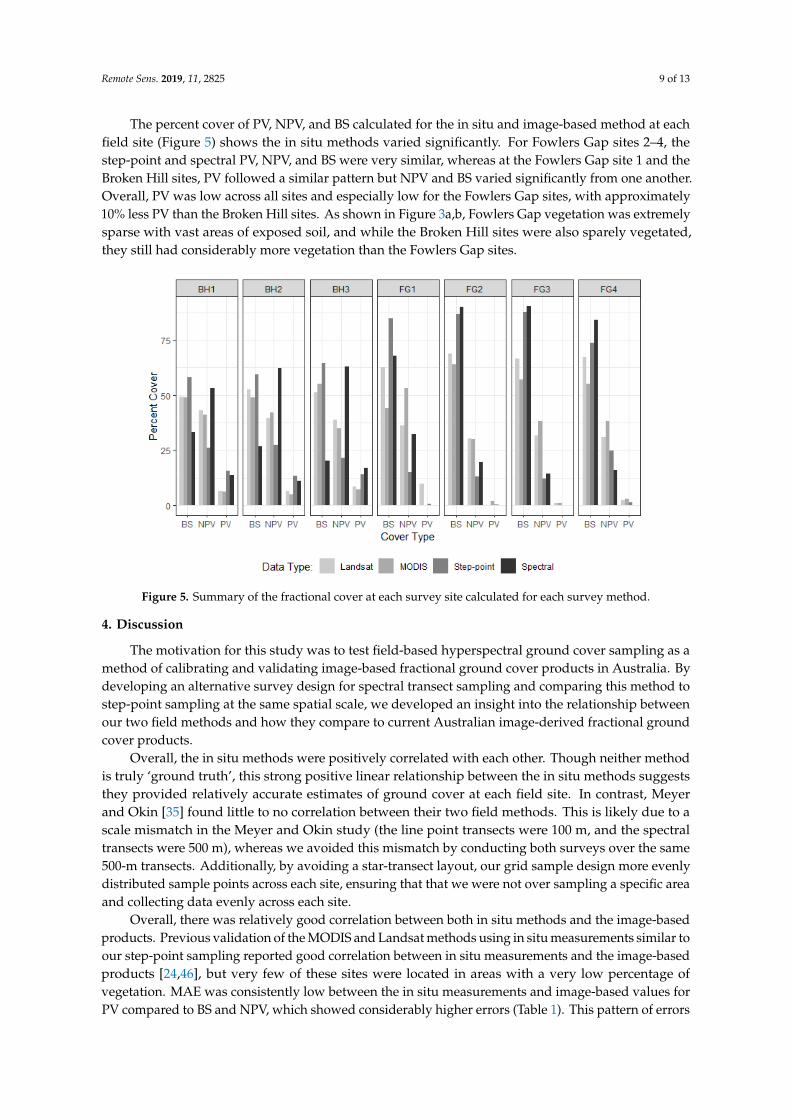
The percent cover of PV, NPV, and BS calculated for the in situ and image-based method at eachfield site (Figure 5) shows the in situ methods varied significantly. For Fowlers Gap sites 2–4, thestep-point and spectral PV, NPV, and BS were very similar, whereas at the Fowlers Gap site 1 and theBroken Hill sites, PV followed a similar pattern but NPV and BS varied significantly from one another.Overall, PV was low across all sites and especially low for the Fowlers Gap sites, with approximately10% less PV than the Broken Hill sites. As shown in Figure 3a,b, Fowlers Gap vegetation was extremelysparse with vast areas of exposed soil, and while the Broken Hill sites were also sparely vegetated,they still had considerably more vegetation than the Fowlers Gap sites.

Remote Sens. 2019, 11, x FOR PEER REVIEW 9 of 13

Step-point Spectral 0.87 1.37 MODIS 0.86 4.24 0.91 4.21 Landsat 0.5 4.68 0.45 4.71

Figure 5. Summary of the fractional cover at each survey site calculated for each survey method.

4. Discussion

The motivation for this study was to test field-based hyperspectral ground cover sampling as a method of calibrating and validating image-based fractional ground cover products in Australia. By developing an alternative survey design for spectral transect sampling and comparing this method to step-point sampling at the same spatial scale, we developed an insight into the relationship between our two field methods and how they compare to current Australian image-derived fractional ground cover products.

Overall, the in situ methods were positively correlated with each other. Though neither method is truly ‘ground truth’, this strong positive linear relationship between the in situ methods suggests they provided relatively accurate estimates of ground cover at each field site. In contrast, Meyer and Okin [35] found little to no correlation between their two field methods. This is likely due to a scale mismatch in the Meyer and Okin study (the line point transects were 100 m, and the spectral transects were 500 m), whereas we avoided this mismatch by conducting both surveys over the same 500-m transects. Additionally, by avoiding a star-transect layout, our grid sample design more evenly distributed sample points across each site, ensuring that that we were not over sampling a specific area and collecting data evenly across each site.

Overall, there was relatively good correlation between both in situ methods and the image-based products. Previous validation of the MODIS and Landsat methods using in situ measurements similar to our step-point sampling reported good correlation between in situ measurements and the image-based products [24,46], but very few of these sites were located in areas with a very low percentage of vegetation. MAE was consistently low between the in situ measurements and image-based values for PV compared to BS and NPV, which showed considerably higher errors (Table 1). This pattern of errors is also consistent with past studies, where PV has been successfully unmixed due to being spectrally unique, whereas BS and NPV are typically harder to distinguish due to their spectral similarity [15,35].

Figure 5. Summary of the fractional cover at each survey site calculated for each survey method.

4. Discussion

The motivation for this study was to test field-based hyperspectral ground cover sampling as amethod of calibrating and validating image-based fractional ground cover products in Australia. Bydeveloping an alternative survey design for spectral transect sampling and comparing this method tostep-point sampling at the same spatial scale, we developed an insight into the relationship betweenour two field methods and how they compare to current Australian image-derived fractional groundcover products.

Overall, the in situ methods were positively correlated with each other. Though neither methodis truly ‘ground truth’, this strong positive linear relationship between the in situ methods suggeststhey provided relatively accurate estimates of ground cover at each field site. In contrast, Meyerand Okin [35] found little to no correlation between their two field methods. This is likely due to ascale mismatch in the Meyer and Okin study (the line point transects were 100 m, and the spectraltransects were 500 m), whereas we avoided this mismatch by conducting both surveys over the same500-m transects. Additionally, by avoiding a star-transect layout, our grid sample design more evenlydistributed sample points across each site, ensuring that that we were not over sampling a specific areaand collecting data evenly across each site.

Overall, there was relatively good correlation between both in situ methods and the image-basedproducts. Previous validation of the MODIS and Landsat methods using in situ measurements similar toour step-point sampling reported good correlation between in situ measurements and the image-basedproducts [24,46], but very few of these sites were located in areas with a very low percentage ofvegetation. MAE was consistently low between the in situ measurements and image-based values forPV compared to BS and NPV, which showed considerably higher errors (Table 1). This pattern of errors

Remote Sens. 2019, 11, 2825 10 of 13

is also consistent with past studies, where PV has been successfully unmixed due to being spectrallyunique, whereas BS and NPV are typically harder to distinguish due to their spectral similarity [15,35].

The observer and the spectral field data recorded less than 1.3% PV at the Fowlers Gap site,MODIS PV values ranged from 0% to 3%, and Landsat ranged from 0% to 9.72% PV. Consideringthe finer resolution of the Landsat product, we would have expected PV to be better correlated withthe Landsat values rather than the MODIS values. A reason for this could be related to the imageproducts. The Landsat FC product is based on a single image captured on one day, whereas the MODISMCD43A4 product calculates the weighted estimate of albedo over a 16-day period. The Landsatimage was captured during this 16-day composite period.

This comparison was conducted with a small number of samples located in the arid zone wherewe know these products tend to fail [19,24]. More extensive surveys are needed to determine if thispattern is more widespread in arid areas. It is also important to remember that we compared singleMODIS pixels with an average of 400 Landsat pixels. Sampling a cluster of pixels is preferable foraccuracy assessment to remove errors associated with positional accuracy [48]. This is feasible forimage products with resolutions of 5, 10, or 30 m but becomes logistically taxing for clusters of MODISpixels at 500 m. This is why the upscaling of field data is regularly used. Currently, the MODIS productis validated using upscaled in situ data initially collected over 100-m transects. Sampling the area of asingle pixel in the field has limitations. We argue that overall, surveying the area of a single MODISpixel is preferable to comparing upscaled field data to a MODIS pixel.

Arid shrublands and desert zone cover 48% of the Australian continent [49]. Having reliablelong-term fractional cover data at varying scales is crucial for those managing or studying theseregions, especially for areas that are inaccessible or unsafe to travel. The in situ methods used haveboth benefits and shortcomings. Step-point sampling has been developed over time as a simple andeasily repeatable method of collecting fractional ground cover estimates. Limitations of this techniqueinclude the time-consuming collection of field observations and the potential for human subjectivityand bias to be introduced, especially when classifying PV and NPV [32]. Utilizing standardizeddefinitions and methods [30] may reduce subjective error but cannot remove it entirely. In order tofurther reduce human bias, spectral transect sampling provides a solution. This method allows forcontinuous, quantitative hyperspectral measurements to be taken over an area, providing an objectiverecord of ground cover without the need for observers to make categorical decisions in the field. Thishyperspectral record of ground cover may also have the potential to calibrate and validate a range ofother remotely sensed products and this is an area of future research. With the continued demand forhigh-quality ground cover products, it is critical to ensure that we are collecting high-quality calibrationand validation data for the assessment of these sought-after products.

5. Conclusions

Field-based estimation of fractional ground cover is critical for ensuring the accuracy andconsistency of remotely sensed ground cover maps. Currently, Australia’s national standard forthe collection of field estimates of ground cover uses traditional field sampling techniques, buthyperspectral reflectance sampling of ground cover has considerable potential to improve fieldmeasurements collected for calibration and validation purposes. This study trailed the use ofhyperspectral reflectance sampling in the sparsely vegetated NSW arid zone. Comparison of step-pointand spectral transect sampling across the same transects, at the same spatial scale, demonstrated thesignificant potential of the spectral transect method, both in is ability to produce results comparableto the traditional transect measures and also in the improved objectivity and relative logistic ease ofthe method.

Overall, we found the in situ step-point and spectral sampling techniques to be positivelycorrelated across the three ground cover classes. Comparing the in situ data and current Australianimage-derived fractional cover products showed that overall, the Landsat product was strongly relatedto both in situ methods for non-photosynthetic vegetation and bare soil whereas the MODIS product

Remote Sens. 2019, 11, 2825 11 of 13

was strongly correlated with both in situ methods for photosynthetic vegetation. These results arespecific to our survey sites and further work is required to test their wider applicability.

While a limitation of spectral sampling is the availability and cost of the spectroradiometer itself,overall, the benefits outweigh the limitations. Spectral sampling is especially beneficial for repeatsurveys or multi-temporal studies. Future efforts should be made to include spectral ground coversampling as part of Australia’s efforts to produce calibration and validation datasets for remotelysensed products and should further test this method to develop a national or global standard.

Author Contributions: Conceptualization, C.F.; methodology, C.F., K.D.C., M.M.L.; data curation, C.F.; formalanalysis, C.F.; writing—original draft preparation, C.F., K.D.C. and M.M.L.; writing—review and editing, C.F.,K.D.C., and M.M.L.

Funding: This research received no external funding.

Acknowledgments: I would like to thank my field assistant Hannah Auricht for giving up her time and for beinggreat company in the field. Thank you to Keith Leggit for granting permission to work on UNSW Fowlers GapResearch Station and to Vikki Dowling for providing excellent accommodation. Lastly, thank you to the BrokenHill City Council and the Rangers at the Living Desert for permission to work on the reserve. Financial supportfor this research was provided by the Australian Government Research Training Program Scholarship and theUniversity of Adelaide School of Biological Sciences.

Conflicts of Interest: The authors declare no conflict of interest.

References

1. Ma, X.; Huete, A.; Yu, Q.; Coupe, N.R.; Davies, K.; Broich, M.; Ratana, P.; Beringer, J.; Hutley, L.B.; Cleverly, J.;et al. Spatial patterns and temporal dynamics in savanna vegetation phenology across the North Australiantropical transect. Remote Sens. Environ. 2013, 139, 97–115. [CrossRef]

2. Gan, M.Y.; Deng, J.S.; Zheng, X.Y.; Hong, Y.; Wang, K. Monitoring urban greenness dynamics using multipleendmember spectral mixture analysis. PLoS ONE 2014, 9, 12. [CrossRef] [PubMed]

3. Quintano, C.; Fernández-Manso, A.; Roberts, D.A. Multiple endmember spectral mixture analysis (mesma)to map burn severity levels from Landsat images in mediterranean countries. Remote Sens. Environ. 2013,136, 76–88. [CrossRef]

4. Mayes, M.T.; Mustard, J.F.; Melillo, J.M. Forest cover change in miombo woodlands: Modeling land cover ofafrican dry tropical forests with linear spectral mixture analysis. Remote Sens. Environ. 2015, 165, 203–215.[CrossRef]

5. Karimi, N.; Golian, S.; Karimi, D. Monitoring deforestation in Iran, Jangal-abr forest using multi-temporalsatellite images and spectral mixture analysis method. Arab. J. Geosci. 2016, 9, 1–16. [CrossRef]

6. Settle, J.; Drake, N. Linear mixing and the estimation of ground cover proportions. Int. J. Remote Sens. 1993,14, 1159–1177. [CrossRef]

7. Smith, M.O.; Ustin, S.L.; Adams, J.B.; Gillespie, A.R. Vegetation in deserts. I. A regional measure of abundancefrom multispectral images. Remote Sens. Environ. 1990, 31, 1–26. [CrossRef]

8. Adams, J.B.; Smith, M.O.; Johnson, P.E. Spectral mixture modeling: A new analysis of rock and soil types atthe viking lander 1 site. J. Geophys. Res. Solid Earth 1986, 91, 8098–8112. [CrossRef]

9. Roberts, D.A.; Gardner, M.; Church, R.; Ustin, S.; Scheer, G.; Green, R.O. Mapping Chaparral in the SantaMonica mountains using multiple endmember spectral mixture models. Remote Sens. Environ. 1998, 65,267–279. [CrossRef]

10. Okin, G.S. Relative spectral mixture analysis—A multitemporal index of total vegetation cover. Remote Sens.Environ. 2007, 106, 467–479. [CrossRef]

11. Baret, F.; Weiss, M.; Lacaze, R.; Camacho, F.; Makhmara, H.; Pacholcyzk, P.; Smets, B. Geov1: Lai and faparessential climate variables and fcover global time series capitalizing over existing products. Part 1: Principlesof development and production. Remote Sens. Environ. 2013, 137, 299–309. [CrossRef]

12. Camacho, F.; Cernicharo, J.; Lacaze, R.; Baret, F.; Weiss, M. Geov1: Lai, fapar essential climate variables andfcover global time series capitalizing over existing products. Part 2: Validation and intercomparison withreference products. Remote Sens. Environ. 2013, 137, 310–329. [CrossRef]

Remote Sens. 2019, 11, 2825 12 of 13

13. Awad, J.; Fisk, C.A.; Cox, J.W.; Anderson, S.J.; van Leeuwen, J. Modelling of THM formation potential andDOM removal based on drinking water catchment characteristics. Sci. Total Environ. 2018, 635, 761–768.[CrossRef] [PubMed]

14. Powell, R.L.; Roberts, D.A.; Dennison, P.E.; Hess, L.L. Sub-pixel mapping of urban land cover using multipleendmember spectral mixture analysis: Manaus, Brazil. Remote Sens. Environ. 2007, 106, 253–267. [CrossRef]

15. Mishra, N.B.; Crews, K.A.; Okin, G.S. Relating spatial patterns of fractional land cover to savanna vegetationmorphology using multi-scale remote sensing in the Central Kalahari. Int. J. Remote Sens. 2014, 35, 2082–2104.

16. Guerschman, J.P.; Hill, M.J.; Renzullo, L.J.; Barrett, D.J.; Marks, A.S.; Botha, E.J. Estimating fractionalcover of photosynthetic vegetation, non-photosynthetic vegetation and bare soil in the Australian tropicalsavanna region upscaling the EO-1 Hyperion and MODIS sensors. Remote Sens. Environ. 2009, 113, 928–945.[CrossRef]

17. Thomas, V.; Treitz, P.; Jelinski, D.; Miller, J.; Lafleur, P.; McCaughey, J.H. Image classification of a northernpeatland complex using spectral and plant community data. Remote Sens. Environ. 2003, 84, 83–99. [CrossRef]

18. Artigas, F.J.; Yang, J.S. Hyperspectral remote sensing of marsh species and plant vigour gradient in the NewJersey meadowlands. Int. J. Remote Sens. 2005, 26, 5209–5220. [CrossRef]

19. Guerschman, J.P.; Oyarzabal, M.; Malthus, T.; McVicar, T.; Byrne, G.; Randall, L.; Stewart, J. Evaluation of theMODIS-Based Vegetation Fractional Cover Product; CSIRO: Canberra, Australia, 2012; pp. 1–28.

20. Lawley, E.F.; Lewis, M.M.; Ostendorf, B. Evaluating MODIS soil fractional cover for arid regions, usingalbedo from high-spatial resolution satellite imagery. Int. J. Remote Sens. 2014, 35, 2028–2046.

21. Montesano, P.; Nelson, R.; Sun, G.; Margolis, H.; Kerber, A.; Ranson, K. MODIS tree cover validation for thecircumpolar taiga–tundra transition zone. Remote Sens. Environ. 2009, 113, 2130–2141. [CrossRef]

22. Morisette, J.T.; Nickeson, J.E.; Davis, P.; Wang, Y.; Tian, Y.; Woodcock, C.E.; Shabanov, N.; Hansen, M.;Cohen, W.B.; Oetter, D.R. High spatial resolution satellite observations for validation of MODIS land products:Ikonos observations acquired under the NASA scientific data purchase. Remote Sens. Environ. 2003, 88,100–110. [CrossRef]

23. Xiao, J.; Moody, A. A comparison of methods for estimating fractional green vegetation cover within adesert-to-upland transition zone in central New Mexico, USA. Remote Sens. Environ. 2005, 98, 237–250.[CrossRef]

24. Scarth, P.; Röder, A.S.M.; Denham, R. Tracking Grazing Pressure and Climate Interaction—The Role ofLandsat Fractional Cover in Time Series Analysis. In Proceedings of the 15th Australasian Remote Sensingand Photogrammetry Conference, Alice Springs, Australia, 13–17 September 2010.

25. Asner, G.P.; Heidebrecht, K.B. Spectral unmixing of vegetation, soil and dry carbon cover in arid regions:Comparing multispectral and hyperspectral observations. Int. J. Remote Sens. 2002, 23, 3939–3958. [CrossRef]

26. Lewis, M.M. Numeric classification as an aid to spectral mapping of vegetation communities. Plant Ecol.1998, 136, 133. [CrossRef]

27. Winkworth, R.; Perry, R.; Rossetti, C. A comparison of methods of estimating plant cover in an arid grasslandcommunity. J. Range Manag. 1962, 194–196. [CrossRef]

28. Graham, F.G. An enhanced wheel-point method for assessing cover, structure and heterogeneity in plantcommunities. J. Range Manag. 1989, 42, 79–81.

29. Evans, R.A.; Love, R.M. The step-point method of sampling-a practical tool in range research. Rangeland Ecol.Manag. J. Range Manag. Arch. 1957, 10, 208–212. [CrossRef]

30. Muir, J.; Schmidt, M.; Tindall, D.; Trevithick, R.; Scarth, P.; Stewart, J. Field measurement of fractional groundcover: A technical handbook supporting ground cover monitoring for Australia. ABARES Canberra ACT2011, 1–58. Available online: https://daff.ent.sirsidynix.net.au/client/en_AU/search/asset/1027474/0 (accessedon 12 July 2017).

31. Trevithick, R.; Muir, J.; Denham, R. The effect of observer experience levels on the variability of fractionalground cover reference data. In Proceedings of the XXII Congress of the International Photogrammetry andRemote Sensing Society, Melbourne, Australia, 25 August–1 September 2012.

32. Fisk, C.; Clarke, K.D.; Delean, S.; Lewis, M.M. Distinguishing photosynthetic and non-photosyntheticvegetation: How do traditional observations and spectral classification compare? Remote Sens. 2019, 11, 2589.[CrossRef]

Remote Sens. 2019, 11, 2825 13 of 13

33. Li, F.; Jupp, D.L.B.; Reddy, S.; Lymburner, L.; Mueller, N.; Tan, P.; Islam, A. An evaluation of the use ofatmospheric and BRDF correction to standardize Landsat data. IEEE J. Sel. Top. Appl. Earth Observ. RemoteSens. 2010, 3, 257–270. [CrossRef]

34. Liang, S.; Fang, H.; Chen, M.; Shuey, C.J.; Walthall, C.; Daughtry, C.; Morisette, J.; Schaaf, C.; Strahler, A.Validating MODIS land surface reflectance and albedo products: Methods and preliminary results. RemoteSens. Environ. 2002, 83, 149–162. [CrossRef]

35. Meyer, T.; Okin, G.S. Evaluation of spectral unmixing techniques using MODIS in a structurally complexsavanna environment for retrieval of green vegetation, nonphotosynthetic vegetation, and soil fractionalcover. Remote Sens. Environ. 2015, 161, 122–130. [CrossRef]

36. Lewis, M. Discrimination of arid vegetation composition with high resolution casi imagery. Rangeland J.2000, 22, 141. [CrossRef]

37. White, A.; Sparrow, B.; Leitch, E.; Foulkes, J.; Flitton, R.; Lowe, A.J.; Caddy-Retalic, S. Ausplots RangelandsSurvey Protocols Manual; University of Adelaide Press: Adelaide, Australia, 2012; Available online: https://www.tern.org.au/AusPlots-Rangelands-Survey-Protocols-Manual-pg23944.html (accessed on 24 August2016).

38. Stern, H.; De Hoedt, G.; Ernst, J. Objective classification of Australian climates. Austr. Meteorol. Mag. 2000,49, 87–96.

39. Bureau of Meteorology. Climate Statistics for Australian Locations—Summary Statistics Fowlers Gap AWS.2019. Available online: http://www.bom.gov.au/climate/averages/tables/cw_046128.shtml (accessed on 12July 2019).

40. Mabbutt, J.A.; Burrell, J.P.; Corbett, J.R.; Sullivan, M.E. Land Systems of Fowlers Gap Station; University of NewSouth Wales: Sydney, Australia, 1973; pp. 25–43.

41. Bureau of Meteorology. Climate Statistics for Australian Locations—Summary Statistics Broken Hill AirportAWS. Available online: http://www.bom.gov.au/climate/averages/tables/cw_047048.shtml (accessed on 12July 2019).

42. Benson, J. Setting the Scene: The Native Vegetation of New South Wales; Background Paper; Native VegetationAdvisory Council: Sydney, Australia, 1999.

43. Analytical Spectral Devices. In Fieldspec 3 User Manual; ASD Inc.: Boulder, Colorado, 2008.44. Gruninger, J.; Ratkowski, A.J.; Hoke, M.L. The Sequential Maximum Angle Convex Cone (Smacc) Endmember

Model; Spectral Sciences Inc.: Burlington, MA, USA, 2004.45. Adams, J.B.; Smith, M.O.; Gillespie, A.R. Imaging spectroscopy: Interpretation based on spectral mixture

analysis. In Remote Geochemical Analysis: Elemental and Mineralogical Composition; Cambridge UniversityPress: New York, NY, USA, 1993; pp. 145–166.

46. Guerschman, J.P.; Hill, M.J. Calibration and validation of the Australian fractional cover product for MODIScollection 6. Remote Sens. Lett. 2018, 9, 696–705. [CrossRef]

47. Geoscience Australia. Fractional Cover (fc25) Product Description. 2015. Available online: https://d28rz98at9flks.cloudfront.net/79676/Fractional_Cover_FC25_v1_5.PDF (accessed on 12 March 2019).

48. Congalton, R.G.; Green, K. Assessing the Accuracy of Remotely Sensed Data: Principles and Practices; CRC Press:Boca Raton, FL, USA, 2008.

49. Department of the Environment. Conservation Management Zones of Australia; Australian Government:Canberra, Australia, 2015.

© 2019 by the authors. Licensee MDPI, Basel, Switzerland. This article is an open accessarticle distributed under the terms and conditions of the Creative Commons Attribution(CC BY) license (http://creativecommons.org/licenses/by/4.0/).