Spatial and temporal point tracking in real hyperspectral images

RESEARCH Open Access

Spatial andtemporal point tracking in realhyperspectral imagesBenjamin Aminov, Ofir Nichtern and Stanley R Rotman*

Abstract

In this article, we consider the problem of tracking a point target moving against a background of sky and clouds.The proposed solution consists of three stages: the first stage transforms the hyperspectral cubes into a two-dimensional (2D) temporal sequence using known point target detection acquisition methods; the second stageinvolves the temporal separation of the 2D sequence into sub-sequences and the usage of a variance filter (VF) todetect the presence of targets using the temporal profile of each pixel in its group, while suppressing clutter-specific influences. This stage creates a new sequence containing a target with a seemingly faster velocity; thethird stage applies the Dynamic Programming Algorithm (DPA) that tracks moving targets with low SNR at aroundpixel velocity. The system is tested on both synthetic and real data.

Keywords: Hyperspectral, Track before detect, Dynamic programming algorithm, Infrared tracking, Variance filter

IntroductionIn the intervening years, interest in hyperspectral sen-sing has increased dramatically, as evidenced byadvances in sensing technology and planning for futurehyperspectral missions, increased availability of hyper-spectral data from airborne and space-based platforms,and development of methods for analyzing data andnew applications [1].This article addresses the problem of tracking a dim

moving point target from a sequence of hyperspectralcubes. The resulting tracking algorithm will be applic-able to many staring technologies such as those used inspace surveillance and missile tracking applications. Inthese applications, the images consist of targets movingat sub-pixel velocities on a background consisting ofevolving clutter and noise. The demand for a low falsealarm rate on the one hand, and a high probability ofdetection on the other makes the tracking a challengingtask. We posit that the use of hyperspectral images willbe superior to current technologies using broadband IRimages due to the ability of the hyperspectral imagetechnique to simultaneously exploit two target-specificproperties: the spectral target characteristics and thetime-dependent target behavior.

The goal of this article is to describe a unique systemfor tracking dim point targets moving at sub-pixel velo-cities in a sequence of hyperspectral cubes or, simplyput, in a hyperspectral movie. Our system uses algo-rithms from two different areas, target detection inhyperspectral imagery [1-9] and target tracking in IRsequences [10-19]. Numerous works have addressedeach of these problems separately, but to the best of ourknowledge, to date no attempts have been made tocombine the two fields.We chose the most intuitive approach to tackle the

problem, namely, divide and conquer; we separate theproblem into three sub-problems and sequentially solveeach one separately. Thus, we first transform eachhyperspectral cube into a two-dimensional (2D) imageusing a hyperspectral target detection method. The nextstep involves a temporal separation of the movie(sequence of images) into sub-movies and the usage of avariance filter (VF) [10-13] algorithm. The filter detectsthe presence of targets from the temporal profile ofeach pixel, while suppressing clutter-specific influences.Finally, a track-before-detect (TBD) approach is imple-mented by a dynamic programming algorithm (DPA), toperform target detection in the time domain [14-17,19].Performance metrics are defined for each step and areused in the analysis and optimization.

* Correspondence: [email protected] of Electrical and Computer Engineering, Ben-Gurion Universityof the Negev, P.O. Box 653, Beer-Sheva 84105, Israel

Aminov et al. EURASIP Journal on Advances in Signal Processing 2011, 2011:30http://asp.eurasipjournals.com/content/2011/1/30

© 2011 Aminov et al; licensee Springer. This is an Open Access article distributed under the terms of the Creative CommonsAttribution License (http://creativecommons.org/licenses/by/2.0), which permits unrestricted use, distribution, and reproduction inany medium, provided the original work is properly cited.

mailto:[email protected]

http://creativecommons.org/licenses/by/2.0

To evaluate the complete system, we need to obtain ahyperspectral movie. Since data of this kind are not yetavailable to us, an algorithm was developed for the creationof a hyperspectral movie, based on a real-world IRsequence and real-world signatures, including an implantedsynthetic moving target, given by Varsano et al. [13].

1 System ArchitectureThe system performs target detection and tracking inthree steps: a match target spectral filter, a sub-pixelvelocity match filter (MF), and a TBD filter. This thirdstep proves to be an effective algorithm for the trackingof moving targets with low signal-to-noise ratios (SNRs).The SNR is defined as:

SNR = MaxT/σ (1)

where MaxT is the target’s maximum peak amplitudeand s is the standard deviation.The general system architecture is given in Figure 1.Parts of this study have been published previously by

our group: we will, therefore, refer extensively to thosepublications. Algorithms for target detection in singlehyperspectral cubes are described in Raviv and Rotman[20], the details of the VF and of the generation of thehyperspectral movie are presented in Varsano et al. [13],and the DPA is described in Nichtern and Rotman [14].In this article, we present an overall integration of thesystem; in particular, the article analyzes the integration

of the VF and the DPA and provides an overall evalua-tion of the system.

Step 1: Transformation of the hyperspectral cube into a2D image - the hyperspectral reduction algorithmThree different reduction tests - spectral average, scalarproduct, and MF - were applied on each temporalhypercube individually. Each of these methods is charac-terized by a mathematical operator, which is calculatedon each pixel. In every frame, a map of pixel scores isobtained (the result of the mathematical operator) andused to create the movie.Test 1: spectral averageThis test involves implementation of a simple spectralaverage of each pixel by:

E (x) =12

∑n

xn (2)

where x denotes the pixel’s spectrum, xn the spectralvalue of the nth band, and N the number of spectralbands.Test 2: scalar productTest 2 is a simple scalar product of the pixel’s spectrum(after mean background subtraction) with the knowntarget spectral signature:

Scalar product = tT · (x − m) (3)

Figure 1 System architecture.


of 25

where x is the pixel being examined, t is the knowntarget signature, and m is the background estimationbased on neighboring pixels.Test 3: MFIn every frame, a map of pixel scores is obtained (theresult of the mathematical operator) and used to createthe movie. The article assumes the linear mixture model(LMM) of the background and a known target signature.The MF detector is given as follows:

MF = tTφ−1(x − m) (4)

where x is the pixel being examined, t is the knowntarget signature, and m and F are the background andcovariance matrix estimations, respectively.The background subtraction procedure is done prior

to applying the filter. The background estimation is per-formed on the closest neighbors that definitely do notcontain the target; for example, if the target is known tobe at most two pixels wide, the background is estimatedfrom the 16 surrounding neighbors, as illustrated inFigure 2.The MF test was run with different target factors

(intensities). The target factor (intensity) can be con-trolled manually by the hyperspectral data creation algo-rithm, as an external parameter to the three testsmentioned previously. A higher target factor value, i.e.,stronger intensity of the implanted target, poses less dif-ficulty to the detection and tracking algorithm. Sincethe target implantation model is linear, it is directly pro-portional to the target factor (intensity of implantation).Overall, the input to the first stage is a hyperspectral

cube; the output of the first stage is a 2D imageobtained from the hypercube. Details of the signal pro-cessing algorithm using a hyperspectral MF can befound in Raviv et al. [20].

Step 2. Temporal separation of the 2D sequence: thetemporal processing algorithmBuffering a number of 2D images acquired in step one isneeded to obtain a sequence that is sufficiently long toperform temporal processing with the VF [13]. Theinput for the temporal processing algorithm is the

temporal profile of a pixel. Figure 3 defines our termi-nology at this stage.The temporal processing algorithm starts with a tem-

poral separation of each temporal profile into sections;each section should roughly cover the time it takes forthe target to enter and leave the pixel. By compressingeach section into a single picture, the original amountof sequence images will now be condensed into a smal-ler sequence of images with the target moving at pixelvelocities (at least one pixel per frame). For example,the profile in Figure 4 (top) is an input to the temporalseparation which increases the velocity of the target toat least one pixel per frame, as shown in Figure 4 (bot-tom). The number of sub-profiles is defined by:

j =N − G0

G − G0(5)

where N is the number of profile frames, G0 is theoverlap between each of the sub-profiles, and G is thelength of the sub-profile.Following temporal separation, the temporal proces-

sing algorithm is applied. The temporal processing algo-rithm is based on a comparison of the sub-profileoverall linear background estimation (defined as DC) tothe single highest fluctuation within the sub-profile. Theoverall linear background estimation (DC) fit, is doneusing a wider temporal window of samples to achievebest background estimation. The background estimationis performed by calculating a linear fit by means of leastsquares estimation (LSE) [21]. The fluctuation or short-term variance estimation is performed on a short tem-poral window of samples (susceptible to temporal varia-tions, i.e., the target entering/leaving pixel), afterremoving the estimated baseline background. The

X X X X X

X

X

X

XX X X X

X

X

X

Examined PixelPixel used for

background estimation

Potentialtarget pixels

Figure 2 Pixels used for background estimation for a target of2 × 2 pixels. Figure 3 Terminology used in Step 2.


of 25

algorithm is presented in the following two steps,although, in practice, the processing can be performedin real time using a finite size buffer.Background estimation using a linear fit modelThe background can be regarded as the DC level ofthe temporal profile: the DC level is constant fornoise-dominated temporal profiles but varies with timewhen clutter is present. The DC is estimated in a pie-cewise fashion using a long-term sliding window andperforming the estimation on each set of samples sepa-rately. The number of samples for each long-term win-dow is denoted by M. The following linear model isused for estimating the DC; for the sake of simplicity,the description of the estimation is applied to a singlewindow:

y = ax + b + n; x = [1, 2, . . .M]T (6)

where n is the noise, a and b are the coefficients thatmust be estimated, M is the number of samples for eachlong-term window, and y is the DC signal. The goal ofthis step is to estimate the long-term DC baseline usinga least-squares fit to the linear model represented by a

coefficients vector [ab]T .

Equation 6 can be rewritten as follows:

y = Xβ + n (7)

where β =[ba

]and X =

⎡⎢⎢⎢⎢⎣

1 11...

1

2...

M

⎤⎥⎥⎥⎥⎦

Using LSE, the following equation is obtained for β :

β = (XTX)−1XTy; β =[ba

](8)

The estimated DC of a single window thus becomes:

y = Xβ (9)

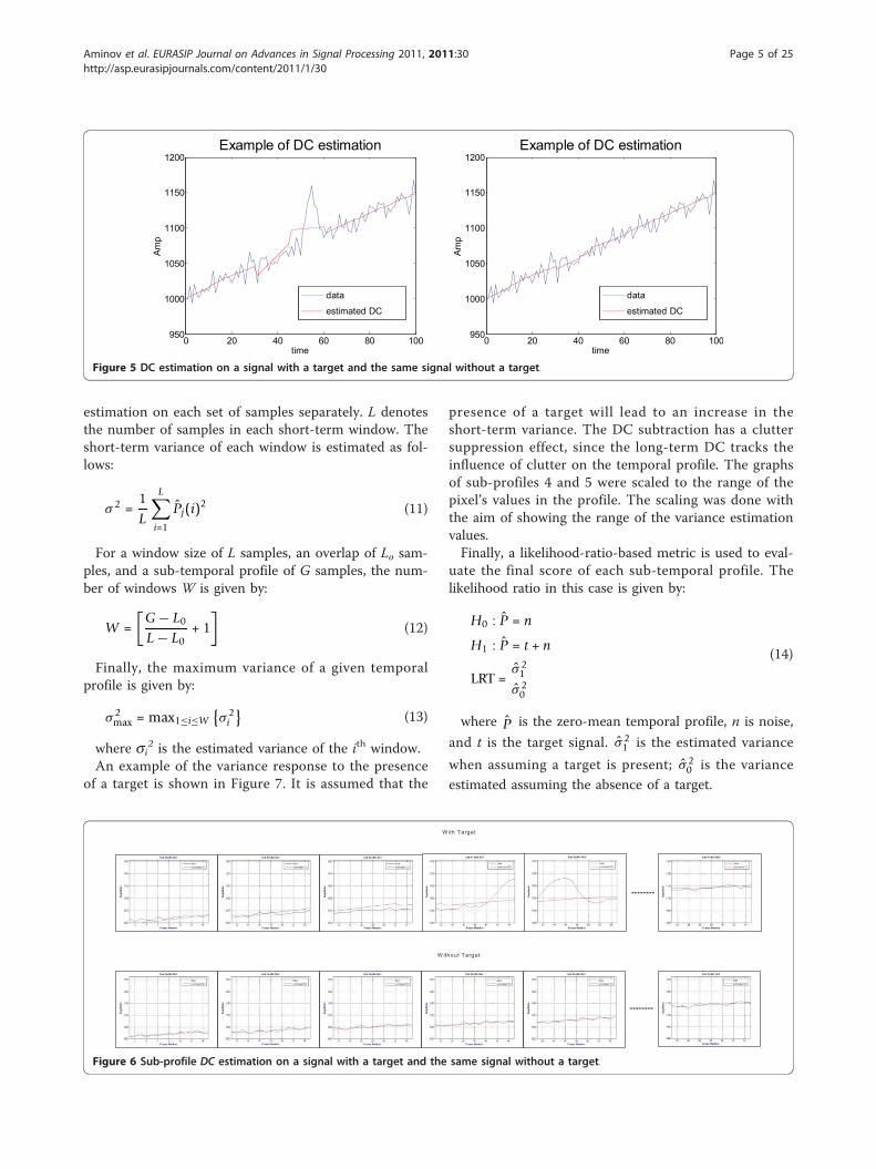
The estimated DC of the complete signal is obtainedafter performing the above calculations for each windowseparately. Figure 5 shows two synthetic temporal pro-files (one with the target implanted and the other withidentical noise but without a target) and their estimatedDC signals.The estimated DC is based on the entire temporal

profile. The sub-profile DC estimation is chosen by therelative location within complete temporal pixel profile.Figure 6 shows the DC estimation on a signal with atarget and the same signal without a target from thepoint of view of the sub-profiles separations.Short-term variance estimationThe short-term variance calculation is performed aftersubtracting the estimated long-term DC from each sub-profile. The complete DC signal obtained in the pre-vious step is denoted by DCj, where j denotes the indexof sub-profile, and the number of sub-profiles is definedin Equation 5. DCj is subtracted from the temporal sub-profile Pj:

P = Pj − DCj (10)

The variance estimation is calculated by using a slid-ing short-term window and performing variance

5 0 5 5 6 0 6 50

5

1 0

1 5

2 0

2 5

3 0

3 5

4 0 4 5 5 0 5 50

5

1 0

1 5

2 0

2 5

3 0

3 5

3 0 3 5 4 0 4 50

5

1 0

1 5

2 0

2 5

3 0

3 5

2 0 2 5 3 0 3 50

5

1 0

1 5

2 0

2 5

3 0

3 5

1 0 1 5 2 0 2 50

5

1 0

1 5

2 0

2 5

3 0

3 5

2 4 6 8 1 0 1 2 1 40

5

1 0

1 5

2 0

2 5

3 0

3 5

Figure 4 Profile with target before (top) and after (bottom) temporal separation.


of 25

estimation on each set of samples separately. L denotesthe number of samples in each short-term window. Theshort-term variance of each window is estimated as fol-lows:

σ 2 =1L

L∑i=1

Pj(i)2 (11)

For a window size of L samples, an overlap of Lo sam-ples, and a sub-temporal profile of G samples, the num-ber of windows W is given by:

W =[G − L0L − L0

+ 1]

(12)

Finally, the maximum variance of a given temporalprofile is given by:

σ 2max = max1≤i≤W

{σ 2i

}(13)

where si2 is the estimated variance of the ith window.An example of the variance response to the presence

of a target is shown in Figure 7. It is assumed that the

presence of a target will lead to an increase in theshort-term variance. The DC subtraction has a cluttersuppression effect, since the long-term DC tracks theinfluence of clutter on the temporal profile. The graphsof sub-profiles 4 and 5 were scaled to the range of thepixel’s values in the profile. The scaling was done withthe aim of showing the range of the variance estimationvalues.Finally, a likelihood-ratio-based metric is used to eval-

uate the final score of each sub-temporal profile. Thelikelihood ratio in this case is given by:

H0 : P = n

H1 : P = t + n

LRT =σ 21

σ 20

(14)

where P is the zero-mean temporal profile, n is noise,

and t is the target signal. σ 21 is the estimated variance

when assuming a target is present; σ 20 is the variance

estimated assuming the absence of a target.

0 20 40 60 80 100950

1000

1050

1100

1150

1200Example of DC estimation

time

Am

p

data

estimated DC

0 20 40 60 80 100950

1000

1050

1100

1150

1200Example of DC estimation

time

Am

p

data

estimated DC

Figure 5 DC estimation on a signal with a target and the same signal without a target.

W ith Target

W ithout Target

Figure 6 Sub-profile DC estimation on a signal with a target and the same signal without a target.


of 25

In our model σ 21 , σ 2

0 variances are estimated as fol-

lows:

σ 21 = σ 2

max

σ 20 =

1K

K∑i=1

σ 2i

(15)

where σ 2i for 1 ≤ i ≤ K denotes the K minimal var-

iance values of each temporal profile. The value of K is

chosen to be smaller than W, so as not to include valuesthat might be caused by the presence of a target.In this case, the final score of each sub-profile is given

by:

Scorej =σ 2max

1K

∑Ki=1 σ 2

i

(16)

The performance of the algorithm depends on a wisechoice of parameters, i.e., the sizes of the short-term

Figure 7 Example of variance estimation on a synthetic signal.


of 25

and long-term windows and the length of the sub-pro-file. The long-term window size serves as the baselinefor DC estimation. Since the pixel might be affected byclutter, the baseline DC is not constant. It is assumedthat the presence of clutter will cause a monotonic riseor fall pattern in the values of the pixel’s temporal pro-file at least during the duration of the long-term win-dow. Thus, the long-term window should be longenough to facilitate accurate estimation of background,on the one hand, and short enough to enable the influ-ence of clutter to be tracked, on the other hand. Thus,the long-term window should be minimally longer thanthe target base width to avoid suppressing it [2]. Theshort-term window is used for variance estimation. Itshould be matched (or reduced) to the target width(which depends on the target velocity). If the short-termwindow is significantly longer than the target width, thechange in variance caused by the target will be reduced.The sub-profile length matches a pixel target velocity; itshould be matched to the target temporal width. Theimportance of these two window sizes and the overallwindow parameters will be discussed in the experimen-tal section of the article. We note that the temporalalgorithm presented here does not assume a particulartarget shape and width. It does, however, assume a max-imum temporal size of the target, (affecting the targettemporal profile), and a positive adding of the targetintensity to the background.To determine the optimal set of window sizes on a

real data sequence, the algorithm was run with varioussets of parameters.

Dynamic Programming AlgorithmThe algorithm is implemented using the followingassumptions [14]:

1. The target size is one pixel or less.2. Only one target exists in each spatial block.3. The target may move in any possible direction.4. Target velocity is within 0-2 pixels per frame(ppf).5. Images are too noisy to allow detection of athreshold on a single frame.6. Jitter of up to 0.5 ppf is allowed only in the hori-zontal and vertical directions and is uniformlydistributed.

Since the target velocity is within the range of 0-2 ppfwith a possible jitter of 0.5 ppf, the pixel can move upto 2.5 ppf in the horizontal and vertical directions;hence, a valid area from which a pixel might originfrom in the previous frame is a 7 × 7 pixel area (matrix).Such a search area can be resized according to differentvelocity ranges and jitter values. The search area will

define the probability matrices that contain the probabil-ities of pixels in the previous frames being the origin ofthe pixel in the current frame. To take into accountunreasonable changes of direction, penalty matrices areintroduced with the aim of building probability matricesfor the different possible directions of movement. Thesematrices give high probabilities to pixels in the esti-mated direction and decreasing probabilities (punish-ment) as the direction varies from the estimateddirection.

2 System EvaluationEvaluation of the temporal algorithm on synthetic dataCreation of synthetic IR framesTo evaluate the performance of the spatial and temporaltracking algorithms, synthetic temporal profiles thatsimulate different types of clutter and background beha-vior were created. A target signal was implanted intothese background signals to simulate a target traversingboth clutter and noise-dominated scenes. On the basisof the study of Silverman et al. [12] showing that thetemporal noise is closely matched to white Gaussiannoise, we used white Gaussian noise at various SNRs totest the temporal algorithm.Figure 8 shows the different types of signal used to

test the algorithm. The type 1 signal shown in Figure 8simulated relatively fast and small clutter formation pas-sing through a pixel. Signals of types 2, 3, and 4 simu-lated, respectively, slowly entering clutter, symmetricalslowly exiting clutter, and a noise-dominated scene inwhich the base timeline is constant. The type 5 signalserved as reference signal, i.e., the best-case scenario,which comprises a constant zero-mean base line.Target temporal profiles were characterized by a rapid

rise and fall pattern. This behavior may be modeled by ahalf sine or triangular shape, as shown in Figure 9.The base width of the target corresponds to the target

velocity. The simulations showed that there were no sig-nificant performance differences between the sine andthe triangular shaped targets.Figure 10 shows the various background models with

the sine shape implanted at an SNR of 4.Examination of the temporal algorithm on synthetic dataThis section demonstrates the algorithm’s operation onthe synthetic data described in the previous section. Thefollowing parameters affect the algorithm’s performance:

1. The background type.2. The SNR, which is a function of the noise var-iance and the target’s amplitude (factor). SNR is afunction of MaxT - the target’s peak amplitude.3. Parameters of the windowing procedure:

a. the window size to estimate the backgroundbaseline DC: the grouping spatial window size to


of 25

convert sub-pixel target velocity to the pixel tar-get velocity in the frame (as an input to theDPA)b. the size of the short-term variance windowsfor each sample and for each groupingc. the step size of each window (overlapping).

The dependence of the performance of the algorithmon these factors is described below.

Background type The factor most influenced by thebackground type is the DC estimation capability of thealgorithm. It is expected that DC estimation will beeasiest for signals having a constant DC level (signals oftypes 4 and 5) and for signals having a slowly changingDC (signals of types 2 and 3), since the linear regressionis capable of estimating parameters of the linear model.Type 1 signals are the most problematic, since the DCof such signals does not have an overall fit with a linear

model, but depends on piecewise matching of the DC towindows sizes, as explained below.Figures 11, 12, 13, 14, 15, 16, 17, 18, 19, and 20 illus-

trate the algorithm’s operation on the various signaltypes, with and without an implemented target. In eachcase, the DC signal and the estimated variance values(calculated after subtracting the estimated DC from thesignal) are also plotted. The simulations were run for aDC window of 20 samples, a DC overlap of 50%, a sub-temporal profile of 15 samples, an overlap between sub-profiles of five samples, and an SNR of 4. The targetwidth was 10 samples.As can been seen in Figure 11, the increase in the var-

iance of sub-profiles 2, 8, and 9 may be attributed to theimprecise DC estimation of the background. This casesimulates a cloud entering and exiting. Nevertheless, thevariance score of the target sub-profiles 5 and 6 is still

Figure 8 Synthetic background signals.


of 25

20 40 60 80 100

0

10

20

30

40

50Sine shaped target

time

ampli

tude

20 40 60 80 100

0

10

20

30

40

50Triangular shaped target

time

ampli

tude

Figure 9 Synthetic target examples.

0 10 20 30 40 50 60 70 80 90 100980

1000

1020

1040

1060

1080

1100

1120

1140

1160

1180Target Type 2 SNR=4

time

ampl

itude

Noisy signalclean signal

0 10 20 30 40 50 60 70 80 90 100980

1000

1020

1040

1060

1080

1100

1120

1140

1160


time

ampl

itude


0 10 20 30 40 50 60 70 80 90 100980

1000

1020

1040

1060

1080

1100

1120


time

ampl

itude


0 10 20 30 40 50 60 70 80 90 100-30

-20

-10

0

10

20

30

40

50


time

ampl

itude


0 10 20 30 40 50 60 70 80 90 100980

990

1000

1010

1020

1030

1040

1050


time

ampl

itude


Figure 10 Example of synthetic signals with an implanted sine target, SNR = 4.


of 25

much higher than that of sub-profiles 2, 8, and 9. Thevariance of the other sub-profiles 1, 3, 4, and 7 is closeto zero.The DC estimation for signals of types 2 and 3 is pre-

cise, since the signal fits a linear model. The variance

increases significantly when the target passes throughthe pixel and is close to zero at other times.Figures 14 and 15 shows a similar behavior for signals

of different DC levels. As expected, the variance of eachof signal (types 4 and 5) is the same.

Figure 11 Example of the temporal algorithm operation on the type 1 signal with a target.


of 25

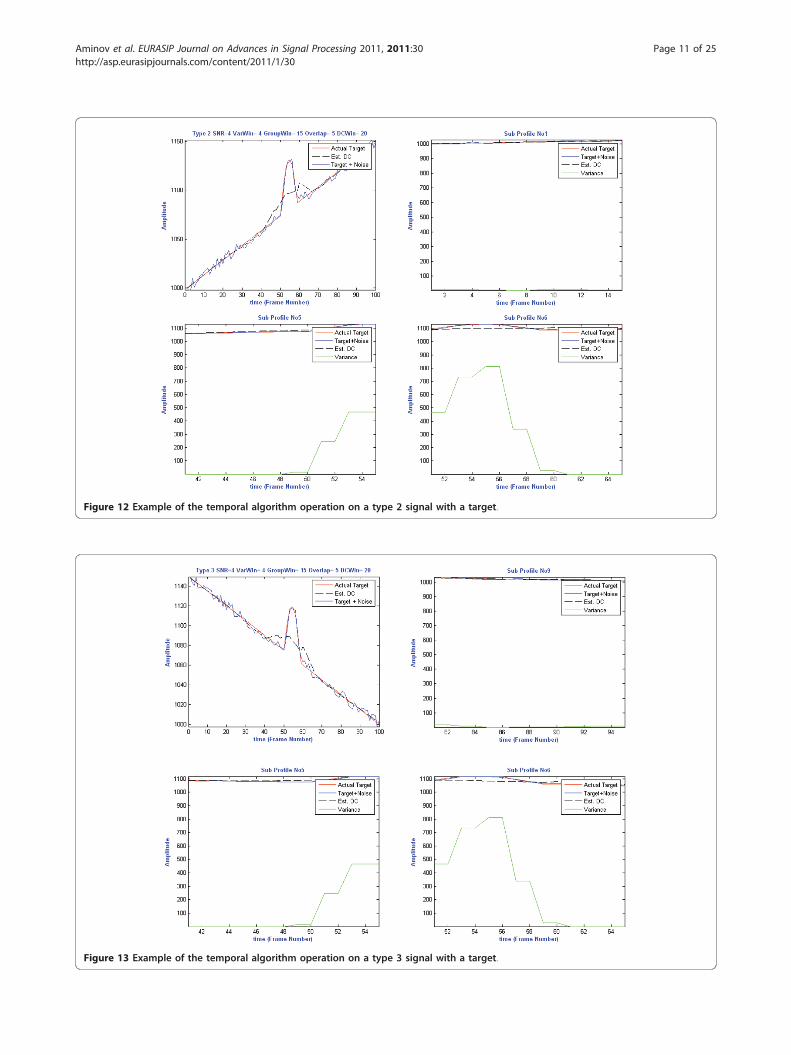
Figure 12 Example of the temporal algorithm operation on a type 2 signal with a target.



of 25

Figures 16, 17, 18, 19, and 20 show the results of tem-poral processing (variance estimation) for the differentsignal types, for the cases where no target is present.Not all the sub-profiles are shown, since the values ofthe exhibited variance values are around zero.From Figure 16 it can be seen that, by analogy with

Figure 11, the variance increases for sub-profiles wherethe cloud enters and exits into/from frame. Such cases,i.e., with no target, may cause false alarms. Figures 17,18, 19, and 20 show that the temporal processing scoreis close to zero for such signals in the absence of atarget.A simple means of performance evaluation is given by

the ratio of the score obtained from the synthetic signalthat contains a target to the same signal without a tar-get, i.e., the target/noise (T/N) ratio. Table 1 shows theT/N ratio for the different signal types obtained by aver-aging 500 runs. It is important to note that the T/Nratio is not an effective metric to evaluate the algorithm,as will be shown later.As expected, the performance of the type 1 signal is

the worst among the different signals. Signals of types2-5 all have similar good performance. If we compareour sub-temporal processing algorithm with a temporalprocessing algorithm as described in [13], it can beclearly seen (Table 1, 2nd column) that the performance

improves by a factor of at least 2 for signals of types 2-5, but not for the type 1 signal, for which the perfor-mance improvement is insignificant.Signal-to-noise ratio As in many other applications, theSNR has a significant influence on the performance ofthe temporal algorithm. As the SNR increases, the algo-rithm’s performance is expected to improve, since boththe DC and variance estimation will be more accurate,as is shown in Figure 21.The algorithm responds similarly for signals of types

2-5, in agreement with expectations, i.e., the perfor-mance improves as the SNR increases. The performanceof the algorithm for the type 1 signal behaves differently;first it increases with the SNR, but at a slower rate thanfor signals of types 2-5, and it then decreases as a resultof an inaccurate DC estimation, as will be detailed later.Since the DC of this signal does not fit a linear modeland the estimation must therefore be performed in pie-cewise fashion, the size and the position of the windowsused to perform the estimation act as a limiting factorto the performance.Window size Both the window size for the baseline DCestimation and the window size for the short-term var-iance for the sub-profile have a marked impact on theperformance of the algorithm. It is expected that largewindow sizes for baseline DC estimation would improve



of 25

the DC estimation in cases where the backgroundchanges monotonically (as for signals of types 2-4). Toolarge a DC estimation window size might, in somecases, lead to inaccurate tracking of the clutter form andcause high false alarm rates (e.g., as for type 1 signals).Thus, for background profiles, the optimal window sizeis determined by the background type, i.e., for a noise-dominated background or backgrounds containingmonotonically changing clutter, larger window sizes arepreferred; for backgrounds characterized by rapidlychanging clutter, shorter windows are preferred. For tar-get temporal profiles, the larger the DC window, thehigher the profile score, since the presence of the targetpeak will have a smaller influence on the DC estimation.Obviously, an estimated DC that tracks the target form

is highly undesirable since it leads to target suppression.Thus, in terms of the overall algorithm performance, theoptimal DC window is the one that is small enough toclosely track background changes but is large enoughnot to track the target peak.The sub-temporal profile length should be matched to

the target sub-pixel velocity, which is expressed as thebase width of the peak of the target profile and the sub-pixel velocity, although there is no acute need for anexact match. The short-term variance window size forthe sub-profile should be matched to the target risetime, although once again there is no acute need for anexact match. A sub-profile length that is larger than thetarget width will disable the ability to track/detect a tar-get with a sub-pixel velocity. Alternatively, a sub-profile



of 25

Figure 16 Example of the temporal algorithm operation on a type 1 signal without a target.



of 25

length that is smaller than the target width will allowtoo few samples for the sub-profile.A short time variance window that is larger than the tar-

get rise time will result in a lower score for the target pro-file, since the variance calculated on each window isnormalized by the window’s length. Thus, for the targetprofile, the optimal variance window size is expected to beless than or equal to the sub-profile length. In fact, theshorter the window, the higher the score of the target pro-file. On the other hand, a short variance window is moresensitive to random noise spikes in a temporal profiledominated by noise. Therefore, the optimal variance win-dow size for noise-dominated profiles should be as largeas possible so as to diminish the effect of the noise spikes.The optimal variance window for the overall algorithm’sperformance is the one offering the best compromisebetween the need to enhance the target profile score (i.e.,as short as possible) and the need to suppress the short-term noise fluctuations (i.e., as long as possible).Another factor which will impact performance is the

overlap window between the sub-profiles. The overlapwindow should allow for the compensation of low sub-pixel velocity that derives from a small sub-profile

length. The overlap window results in the creation ofmore sub-profiles, as defined in Equation 5, since thegreater number of sub-profiles aids to achieve a moreaccurate tracking estimation.

Evaluation of the temporal processing algorithm on realdataReal IR sequencesReal-world IR image sequences taken from Silverman etal. [22] were used for evaluating the temporal algorithm.The movies comprised 95 or 100 12-bit IR frames. Thesequences contain raw data of unresolved targets flyingfrom Boston Logan Airport in Massachusetts, USA. Inthe available dataset, there are five scenes containingvarious types of clutter and sky as well as various targetsmoving at different velocities.Figure 22 shows a single frame (frame 50) of each of

the IR sequences examined in this study. Table 2 sum-marizes the number and the nature of the targets foreach IR sequence and the background type of scene.Evaluation metricsSilverman et al. [22] suggested several performancemetrics for the evaluation of temporal algorithms. A




of 25

derived version of the metric was defined. Each frame inthe sequence was divided into H × N blocks (30 × 30were used), and the algorithm was run over nine blocks,i.e., the target block (TB) and its eight adjacent non-tar-get blocks (NTB). The SNRs of the TB and its eightadjacent NTBs were calculated. Thereafter, the algo-rithm score was calculated on the basis of the resultingSNRs.The block SNR is given as:

Block SNR(i, j) =E[vi,j ∈ M] − E[vi,j /∈ M]

σvi,j(17)

where vi, j is the set of pixels belonging to the (i, j)th

block, M is a set containing the five pixels with thehighest gray level in that block, s is the standard devia-tion of the block pixels. E[vi, j Î M] is the expectedvalue of the highest pixels (target) and the E[vi, j ∉ M] isthe expected value of the rest of the pixels(background).The algorithm score is given as:

Score =Block SNR(i, j)(i,j)=TB − E

[{Block SNR(i, j)(i,j)=NTB

}]σ{

Block SNR(i,j)(i,j)=NTB

} (18)

The block formula performs a subtraction between theexpectation value of the highest pixels (target) and theexpectation value of the rest of the pixels (background),divided by the standard deviation of block pixels. Sincethe probability matrices of the DPA introduce the

influence of target pixels on adjacent pixels, these influ-enced pixels might accumulate higher values than unaf-fected pixels (background), and can be regarded astarget pixels. This might lower the expectation value ofthe target, but will also lower the standard deviation ofthe background, since these high pixels are higher thanthe statistics of the background.The final grade of the algorithm serves as a tool for

comparison between the suggested temporal processingalgorithm and other temporal processing algorithmsthat deal with the same problems. The grade is a reflec-tion of the difference between the score of the blockcontaining the target and the expected values of the restof the blocks in the image, normalized by their standarddeviations.Real data resultsThe real-world IR image sequences described in the pre-vious section were used to evaluate the temporal track-ing algorithm. The algorithm’s output images are givenin Figure 23, together with a representative frame fromeach sequence. The sequences were chosen so as to


Table 1 Target/noise (T/N) ratio for various signal types

Signal type T/N ratio T/N ratio [Varsano et al. [13]]

1 1.8098 1.72

2 10.9558 4.34

3 10.9658 4.41

4 10.9659 4.29

5 10.9659 4.41 Figure 21 T/N ratio versus SNR for different signal types.


of 25

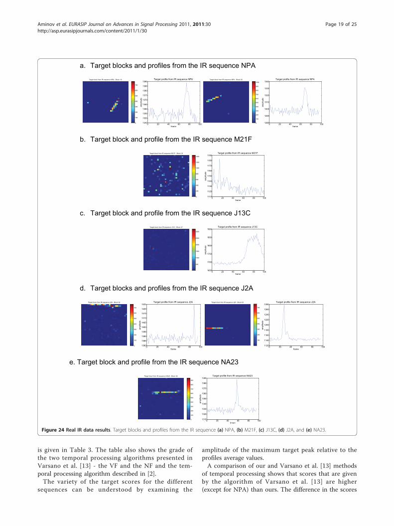
comprise both clutter- and noise-dominated scenes. Theparameters of each simulation were chosen to be theoptimal set, as will be explained in the following section.The target tracks are seen as bright short stripes, and insome cases, clutter leakage is also evident.Figure 24 provides a closer view of the block contain-

ing the target of each output image together with a

representative target temporal profile. Visual evaluationof the images presented in Figure 24 suggests that interms of enhancement of the target pixels, the bestresults were obtained for the sequences J2A and NPA,since the target trace is stronger relative to the back-ground. The M21F sequence, for example, has morenoise in the background, although the target pixels areclearly visible. The metric defined for assessing the over-all performance of the algorithm, which is given inEquation 17, takes into consideration not only the targetenhancement but also the ability of the algorithm tosuppress the background. This is achieved by gradingeach block with a score that evaluates the differencebetween the maximal 5 values of the block and theblock average values, normalized by the standard

The IR image NPA

1300

1350

1400

1450

1500

1550

1600

1650

The IR image J13C

1800

2000

2200

2400

2600The IR image NA23

1200

1400

1600

1800

2000

2200

The IR image J2A

1100

1200

1300

1400

1500

1600 The IR image M21F

1050

1100

1150

1200

Figure 22 Frame 50 of each real data IR sequence.

Table 2 Description of the IR sequences

IR sequence Scene description

NPA Two targets in wispy clouds

J13C One slow target in clear of cloudy scene

NA23 One fast target in bright clouds

J2A Two targets in fluffy clouds

M21F One weak target in hot hazy night sky


of 25

deviation. The goal is, of course, to obtain TBs withhigh scores and background blocks with low scores.The purpose of the final grading of the algorithm,

defined in Equation 18 is to evaluate the separationbetween the TB(s) and the background blocks. The

grading provides an evaluation of the difference betweenthe TB score (and if there is more than one target, themean of the TBs) and the mean of the backgroundblocks, normalized by the standard deviation of thebackground. The final grade obtained for each sequence

Frame 70 from IR sequence NPA Result Image of IR sequence NPA

Frame 70 from IR sequence J13C Result Image of IR sequence J13C

Frame 70 from IR sequence M21F Result Image of IR sequence M21F

Frame 70 from IR sequence J2A Result Image of IR sequence J2A

Frame 70 from IR sequence NA23 Result Image of IR sequence NA23

Figure 23 Output images of the temporal tracking algorithm.


of 25

is given in Table 3. The table also shows the grade ofthe two temporal processing algorithms presented inVarsano et al. [13] - the VF and the NF and the tem-poral processing algorithm described in [2].The variety of the target scores for the different

sequences can be understood by examining the

amplitude of the maximum target peak relative to theprofiles average values.A comparison of our and Varsano et al. [13] methods

of temporal processing shows that scores that are givenby the algorithm of Varsano et al. [13] are higher(except for NPA) than ours. The difference in the scores

a. Target blocks and profiles from the IR sequence NPA

b. Target block and profile from the IR sequence M21F

c. Target block and profile from the IR sequence J13C

d. Target blocks and profiles from the IR sequence J2A

e. Target block and profile from the IR sequence NA23

Target block from IR sequence NPA - Block 16

0

100

200

300

400

500

600

700

0 20 40 60 80 1001345

1350

1355

1360

1365

1370

1375

1380

1385

1390Target profile from IR sequence NPA

frame

ampl

itude

Target block from IR sequence NPA - Block 55

0

100

200

300

400

500

600

700

800

900

1000

0 20 40 60 80 1001280

1290

1300

1310

1320

1330

1340Target profile from IR sequence NPA

frame

ampl

itude

Target block from IR sequence M21F - Block 33

0

200

400

600

800

1000

1200

1400

0 20 40 60 80 1001110

1120

1130

1140

1150

1160

1170

1180

1190Target profile from IR sequence M21F

frame

ampl

itude

Target block from IR sequence J13C - Block 47

500

1000

1500

2000

2500

3000

0 20 40 60 80 1001650

1700

1750

1800

1850

1900Target profile from IR sequence J13C

frame

ampl

itude

Target block from IR sequence J2A - Block 42

0

100

200

300

400

500

600

700

0 20 40 60 80 1001380

1385

1390

1395

1400

1405

1410

1415

1420

1425Target profile from IR sequence J2A

frame

ampl

itude

Target block from IR sequence J2A - Block 63

100

200

300

400

500

600

700

0 20 40 60 80 1001120

1140

1160

1180

1200

1220

1240

1260

1280Target profile from IR sequence J2A

frame

ampl

itude

Target block from IR sequence NA23 - Block 26

0

100

200

300

400

500

600

700

800

900

0 20 40 60 80 1001310

1320

1330

1340

1350

1360

1370

1380

1390Target profile from IR sequence NA23

frame

ampl

itude

Figure 24 Real IR data results. Target blocks and profiles from the IR sequence (a) NPA, (b) M21F, (c) J13C, (d) J2A, and (e) NA23.


of 25

may be attributed to the differences in the metrics andTP calculation, i.e., the difference in the metric calcula-tion is due to the fact that we have more score framesand hence we calculate their average, as described atFigure 25 and 25 in Table 1; the temporal processingmethod used gives us a better target to noise ratio.The sequences in NPA differ from those in NA23:

although the target in NPA seems weaker, its blockscore is higher than that of NA23 as a result of thestrong clutter in the NA23 scene as shown at Table 4.As stated in the following section, the window size para-meters are not optimized in terms of both the TB andthe background. Thus, choosing an inappropriate win-dow size will lower the TB score. Therefore, althoughthe target in NA23 is stronger than that in NPA, the TBscore obtained after the temporal processing is lower.Finally, the lowest target score is that for the M21Fsequence. The target here is quite weak, and the sceneis noise dominated, hence the low target amplitude andthe low TB score. The algorithm score for this sequencewas the lowest among the scores of all the sequences.Optimal window sizeChoosing the appropriate set of parameters for the tem-poral algorithm is crucial for the detection capabilitiesof the system. The dependence of the algorithm on thewindow size was evaluated on real data, and the optimalset of parameters was obtained for each IR sequence.The expected optimal window sizes depend on both

the shape of the target’s temporal profile, mainly on thetarget’s peak width, which is inversely proportional to

the target’s velocity, and on the background scene, i.e.,on the presence of clouds and their size and velocity, asstated in section “Window size”.To determine the optimal set of window sizes on a

real data sequence, the algorithm was run on thesequence with various sets of parameters. The set thatyielded the highest algorithm grade, defined in Equation18, was chosen for the evaluation.Figure 26 shows the results of the simulation on the

IR sequence NPA. The results show that the highestalgorithm score was obtained for a group width of size14 samples, an overlap of size 7 samples and a variancewindow of size 6 samples with a linear (DC) window ofsize 50 samples. The final algorithm grade provides anevaluation of the difference between the target’s blockscore (if there is more than one target, the relevantscores are averaged) and the mean background score,normalized by the standard deviation of the backgroundblocks. Thus, the optimal window set will tend to maxi-mize the target score while minimizing the backgroundand standard deviation scores. Table 5 summarizes theoptimal window sets for three IR sequences.

Evaluation of the complete system on real dataThe hyperspectral movie is created as described in Var-sano et al. [13]. The movie consists of a sequence of 30× 30 × 96 cubes (width × height × bands). A synthetictarget is implanted into the sequence. The target is sine-shaped, 2 × 2 pixels wide, and has a horizontal and ver-tical velocity of 0.1 ppf. White Gaussian noise is addedto each spectral signature and the noise variance is setto be [0.1 × Max(signature)]2.The movie then constitutes the input into our system.

The MF with the estimated covariance matrix is appliedfor the first-stage processing of each hypercube, and thetemporal processing algorithm described in section “Sys-tem architecture” is used for the target detection in thesecond stage. The output of the second stage constitutesthe input into the DPA. The DPA allows us to track the

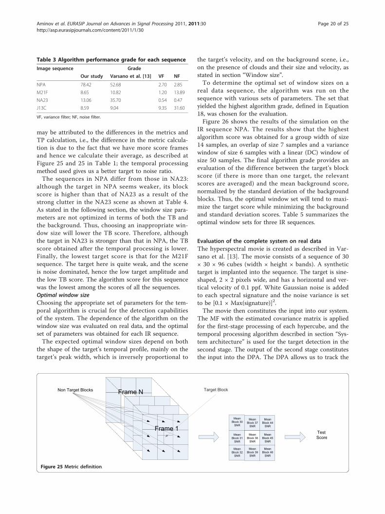
Table 3 Algorithm performance grade for each sequence

Image sequence Grade

Our study Varsano et al. [13] VF NF

NPA 78.42 52.68 2.70 2.85

M21F 8.65 10.82 1.20 13.89

NA23 13.06 35.70 0.54 0.47

J13C 8.59 9.04 9.35 31.60

VF, variance filter; NF, noise filter.

Target BlockNon Target Blocks

Frame 1

Frame N

Mean Block 30

SNR

Mean Block 39

SNR

Mean Block 44

SNR

Mean Block 31

SNR

Mean Block 38

SNR

Mean Block 32

SNR

Mean Block 37

SNR

Mean Block 45

SNR

Mean Block 46

SNR

TestScore

Figure 25 Metric definition.


of 25

target from pixel to pixel; an updated summation scorefor each pixel is kept for each pixel, based on its similar-ity to expected target behavior. Penalties are introducedto lower the score of pixels apparently acting in a non-physical manner. In the final stage, the last processedframe is taken and the highest pixel is declared as a“target” and its track is found. In this section, we willdefine three tests to evaluate the effect of each stage ofthe algorithm.Metric definitionThe performance metric, Equations 17 and 18, was usedto evaluate various stages of the analysis. The three testsbased on this metric were applied. Test 3 uses a MF forthe cube collapsing. The resulting cubes are then evalu-ated as described in Equations 17 and 18; the cube with

the highest score will be evaluated as representative ofthe efficacy of using the MF alone.Test 4 (full system test) uses a MF detector as the

input of the temporal processing velocity filter. Test 5(full system test) adds to Test 4 the DPA. These testswere created to evaluate the effect of the IR trackingalgorithms on the overall score of the hyperspectraltracking system.The MF and the temporal processing algorithm create

images with pixel scores according to their likelihood ofbeing a target, whereas the DPA accumulates the scoresof pixels according to the probability of the path goingthrough them to be the target’s path.

Discussion of the results obtained on real dataHere, we present the results of applying the completesystem algorithm on a hyperspectral movie based onblocks from the real IR sequence NA23. The algorithm

Table 4 Target maximal peak for the different IRsequences

Sequence Target peak

NPA Approximately 30

J2A Approximately 140

M21F Approximately 18

NA23 Approximately 60

J13C Approximately 150

Figure 26 Algorithm score versus window size sets for the IR sequence NPA.

Table 5 Optimal window sets for three IR sequences

Sequence Group width Overlap Variance window

NPA 14 7 6

M21F 19 18 8

NA23 16 5 4


of 25

was run on TBs and their eight surrounding backgroundblocks. The blocks were chosen to represent three dif-ferent scenes, which could roughly be categorized as“clear sky” (containing only sky), “weak clutter” (con-taining partial weak clutter (with low to medium IRamplitude)) and “strong clutter” (containing partial clut-ter with high IR amplitudes). The parameters of thesimulation are summarized in Table 6.Tables 7, 8, 9, 10, and 11 present the results for

hypercubes of three different backgrounds, based onblocks from the real IR sequence NA23. Figure 27shows a single frame from the sequence, divided intolabeled blocks.Comparison of Tables 9 and 10 shows that scores for

Test 4 were lower than those for Test 3. This differencemay be attributed to differences in the calculation of themetrics and the temporal processing method, i.e., thedifference in the metric calculation due to the fact that

we have more score frames and hence calculate theiravarage (Figure 25); and as described in Table 1, thetemporal processing method used gives us a better targetto noise ratio.Previous research [13] has shown that Test 1 allows a

rough assessment of the relative amplitude of the targetpixels vis-à-vis their background. The low values of theresults indicate that the implantation of the target andtaking the maximal score without any processing is notsufficient for target detection; in other words, theimplantation method does not allow an “easy” detection.The highest values of Test 1 were obtained for the weakclutter scenes, which is reasonable since the implanta-tion method is additive and in weak clutter surround-ings, the amplitudes are obviously higher than those inclear sky scenes. A comparison of Tests 1 and 2 allowedus to estimate the improvement conferred by using pri-mitive hyperspectral processing, i.e., simply taking theaverage of all the bands. Although this method led to animprovement in the sky and weak clutter scenes, it hadnegative impact on strong clutter scenes, a finding thatindicates that simply averaging the bands is disastrousfor certain sets of spectral signatures and cannot itselfbe used as a detection method. Thus, the discussion willfocus on the use of “smart” hyperspectral processing(Test 3), hyperspectral processing and temporal proces-sing (Test 4), and hyperspectral processing, temporalprocessing and the DPA (Test 5). The results of Varsanoet al. [13] have shown that there is an obvious advantageof using both hyperspectral detection (MF) and tem-poral processing (Test 4 vs. Tests 1-3).When the target is implanted in clear sky scenes, the

use of temporal processing significantly improves theperformance vis-à-vis hyperspectral detection alone. Inmost cases, the use of the MF compared to simple aver-aging was clearly advantageous, with the exception of

Table 6 Complete system simulation parameters

Parameter Value

Hyperspectral movie parameters

Movie length 95 frames

Spectral signatures Identical to the ones presented in Varsano et al.[13], Figure 13

Block size 30 × 30 pixels

Number ofspectral bands

100 bands

IR sourcesequence

NA23, taken from Silverman et al. [23]

Noise added White Gaussian noise factor of 0.05 (std = noisefactor * 0.05)

Synthetic target properties

Spatial shape Half sine, 2 × 2 pixels, integral of the spatialdistribution normalized to 0.5

Horizontal velocity 1/8 pixels/frame

Vertical velocity 1/8 pixels/frame

Velocity error Noise factor of 0.25, as described in Varsano et al.[13], section 6.3

Hyperspectral cube reduction

Reduction filter Match filter, selected according to bestperformance

Target block 37 (weak clutter), 38 (sky only), 39 (strong clutter)

Target factor 10, 20, 40, 60, 80, 100, 500, 1000

Temporal processing parameters

Sub profile length 15 samples

Overlap 10 samples

DC window 50 samples

DC step size 15 samples

Variance window 4 samples

DPA

EMC (b) [0...6] for g = 0, [0...1] for g = 1

a 1

p 0.5

y 24

Table 7 Evaluation results of Test 1-spectral average

Block Scene Target factor

Description 20 40 60 80

37 Partial weak clutter 1.7622 1.7542 1.7414 1.7204

38 Mainly sky -1.3432 -1.0566 -0.5864 -0.0326

39 Mainly strong clutter -0.0362 -0.0371 -0.0354 -0.0392

Mean 0.1276 0.2201 0.3732 0.5495

Table 8 Evaluation results of Test 2-scalar product




38 Mainly sky -1.2325 -0.8918 -0.3695 0.2114


Mean -0.3548 -0.2575 -0.0712 0.1470


of 25

block 31, for which the performance was similar for thetwo techniques. This similarity may be attributed to therelative “easiness” of detection in this kind of scene andthe fact that the high level of noise might confer a dis-advantage on the MF but an advantage on the averagingfilter. When weak clutter was present, temporal proces-sing combined with the MF detector was always betterthan hyperspectral detection alone.A parameter known as the target factor (MaxT) has

been used to describe linearly the power in the targetsignature. To define the boundaries of the full system, itis necessary to define a valid range for the target factor.Preliminary runs for target factors of 1000, 500, 100,and 10 showed that target factors of ≥ 100 are “tooeasy” to use a detection algorithm, whereas a target fac-tor of 10 is “too hard” for the full system to detect andtrack a target. Therefore, trial runs were performed withthe following values of the target factor: 20-80 withsteps of 20. Figures 28 and 29 show the results for block38 for target factors of 100 and 20, respectively, for var-ious stages.

3 ConclusionsIn this study, a complete system for the tracking of dimpoint targets moving at sub-pixel velocities in a sequenceof hyperspectral cubes or, simply put, a hyperspectralmovie was presented. Our research incorporates algo-rithms from two different areas, target detection in hyper-spectral imagery and target tracking in IR sequences.

Table 9 Evaluation results of Test 3 - Match filter




38 Mainly sky -0.2196 0.2049 0.7912 1.3592


Mean 0.62317 0.7512 0.9690 1.1916

Table 10 Evaluation results of Test 4-match filter andtemporal processing




38 Mainly sky 3.2252 3.6421 3.7222 3.7188

39 Mainly strong clutter 0.5539 1.6206 3.1649 3.4353

Mean 2.2404 2.9817 3.5356 3.6204

Table 11 Evaluation results of Test 5-match filter,temporal processing and DPA




38 Mainly sky 3.7568 3.8255 3.8318 3.8365

39 Mainly strong clutter 2.0955 2.3476 3.7458 3.7171

Mean 3.1665 3.3312 3.8008 3.7994

The IR image sequence NA23, Frame 1

1

2

3

4

5

6

7

8

9

10

11

12

13

14

15

16

17

18

19

20

21

22

23

24

25

26

27

28

29

30

31

32

33

34

35

36

37

38

39

40

41

42

43

44

45

46

47

48

49

50

51

52

53

54

55

56

57

58

59

60

61

62

63

64

65

66

67

68

69

70

1200

1300

1400

1500

1600

1700

1800

1900

2000

2100

2200

Figure 27 Single frame of IR sequence NA23 with labeled blocks division.


of 25

(a) (b)

-1

-0.5

0

0.5

1

1.5

2

2.5

3

3.5

10

20

30

40

50

60

70

80

Figure 28 Block 38, target factor 100: (a) single frame after MF (Test 1), (b) single frame after MF and TP (Test 2).

(a) (b)

(c)

-0.8

-0.6

-0.4

-0.2

0

0.2

0.4

0.6

0.8

20

40

60

80

100

120

140

160

180

200

220

5 10 15 20 25 30

5

10

15

20

25

30

50

100

150

200

Figure 29 Block 38, target factor 20: (a) single frame after MF (Test 1-Frame 64), (b) single frame after MF and TP (Test 2-Frame 12), (c) singleframe after MF, TP, and DPA (Test 3-Frame 12).


of 25

Performance metrics are defined for each step and areused in the analysis and optimization; a comparison ismade to previous work in this area.

AbbreviationsDPA: dynamic programming algorithm; LSE: least squares estimation; LMM:linear mixture model; MF: match filter; NTB: non-target block; SNRs: signal-to-noise ratios; TB: target block; TBD: track-before-detect; 2D: two-dimensional;VF: variance filter.

Competing interestsThe authors declare that they have no competing interests.

Received: 22 March 2010 Accepted: 26 July 2011Published: 26 July 2011

References1. J Chanussot, MM Crawford, BC Kuo, Foreword to the special issue on

hyperspectral image and signal processing. IEEE Trans Geosci Remote Sens.48(11), (2010)

2. G Shaw, D Manolakis, Signal processing for hyperspectral imageexploitation. IEEE Signal Process Mag. 19, 12–16 (2002)

3. D Landgrebe, Hyperspectral image data analysis as a high dimensionalsignal processing problem. IEEE Signal Process Mag. 19, 17–28 (2002)

4. G Shaw, H Burke, Spectral imaging for remote sensing. Lincoln Lab J. 14(1),3–27 (2003)

5. CE Caefer, SR Rotman, J Silverman, PW Yip, Algorithms for point targetdetection in hyperspectral imagery. Proc SPIE. 4816, 242–257 (2002)

6. D Manolakis, G Shaw, Detection algorithms for hyperspectral imagingapplications. IEEE Signal Process Mag. 19, 29–43 (2002). doi:10.1109/79.974724

7. N Keshava, JF Mustard, Spectral unmixing. IEEE Signal Process Mag. 19,44–57 (2002). doi:10.1109/79.974727

8. DWJ Stein, SG Beaven, LE Hoff, EM Winter, AP Schaum, AD Stocker,Anomaly detection from hyperspectral imagery. IEEE Signal Process Mag.19, 58–69 (2002). doi:10.1109/79.974730

9. O Duran, M Petrou, A time-efficient method for anomaly detection inhyperspectral images. IEEE Trans Geosci Remote Sens. 45, 3894–3904 (2007)

10. CE Caefer, JM Mooney, J Silverman, Point target detection in consecutiveframe staring IR imagery with evolving cloud clutter. Proc SPIE. 2561, 14–24(1995)

11. CE Caefer, J Silverman, JM Mooney, S DiSalvo, RW Taylor, Temporal filteringfor point target detection in staring IR imagery: I. damped sinusoid filters.Proc SPIE. 3373, 111–122 (1998)

12. J Silverman, CE Caefer, S DiSalvo, VE Vickers, Temporal filtering for pointtarget detection in staring IR imagery: II. Recursive variance filter. Proc SPIE.3373, 44–53 (1998)

13. L Varsano, I Yatskaer, SR Rotman, Temporal target tracking in hyperspectralimages. Opt Eng. 45(12), 126201 (2006). doi:10.1117/1.2402139

14. O Nichtern, SR Rotman, Point target tracking in a whitened IR sequence ofimages using dynamic programming approach. Proc SPIE 6395, Electro-Optical and Infrared Systems: Technology and Applications III, 63950U, ed. byDriggers RG, Huckridge DA, (September 2006)

15. Y Barniv, Dynamic Programming solution for detecting dim moving targets.Aerospace Electron Syst Proc IEEE. 29(1), 44–56 (1985)

16. Y Barniv, O Kella, Dynamic programming solution for detecting dim movingtargets part II: analysis. Aerospace Electron Syst Proc IEEE. 23(6), 776–788(1987)

17. J Arnold, H Pasternack, Detection and tracking of low observable targetsthrough dynamic programming. Proc SPIE Signal Data Process SmallTargets. 1305, 207–217 (1990)

18. R Succary, H Kalmanovitch, Y Shurnik, Y Cohen, E Cohen, SR Rotman, Pointtarget detection. Infrared Technol Appl XXVII Proc SPIE. 3820, 671–675(2003)

19. R Succary, A Cohen, P Yaractzi, SR Rotman, A dynamic programmingalgorithm for point target detection: practical parameters for DPA. SignalData Process Small Targets Proc SPIE. 4473, 96–100 (2001)

20. O Raviv, SR Rotman, An improved filter for point target detection in multi-dimensional imagery. Proc of SPIE Imaging Spectrometry IX, ed. by Shen SS,Lewis PE 5159, 32–40 (2003)

21. S Chatterjee, AS Hadi, Influential observations, high leverage points, andoutliers in linear regression. Stat Sci. 1(3), 379–416 (1986). doi:10.1214/ss/1177013622

22. J Silverman, CE Caefer, JM Mooney, Performance metrics for point targetdetection in consecutive frame IR imagery. Proc SPIE. 2561, 25–30 (1995)

23. IR Source Sequences, http://www.sn.afrl.af.mil/pages/SNH/ir_sensor_branch/sequences.html

doi:10.1186/1687-6180-2011-30Cite this article as: Aminov et al.: Spatial andtemporal point tracking inreal hyperspectral images. EURASIP Journal on Advances in SignalProcessing 2011 2011:30.

Submit your manuscript to a journal and benefi t from:

7 Convenient online submission

7 Rigorous peer review

7 Immediate publication on acceptance

7 Open access: articles freely available online

7 High visibility within the fi eld

7 Retaining the copyright to your article

Submit your next manuscript at 7 springeropen.com


of 25

http://www.sn.afrl.af.mil/pages/SNH/ir_sensor_branch/sequences.html

http://www.sn.afrl.af.mil/pages/SNH/ir_sensor_branch/sequences.html

http://www.springeropen.com/

http://www.springeropen.com/

Spatial and temporal point tracking in real hyperspectral images

Documents

Transcript of Spatial and temporal point tracking in real hyperspectral images