Purdue UniversityPurdue e-Pubs

ECE Technical Reports Electrical and Computer Engineering

2-21-2007

Border Feature Detection and Adaptation forClassification of Multispectral and HyperspectralRemote Sensing ImagesN. Gokhan KasapogluInstanbul Technical University, gokhank@itu.edu.tr

okan ersoyersoy@purdue.edu

Follow this and additional works at: http://docs.lib.purdue.edu/ecetr

This document has been made available through Purdue e-Pubs, a service of the Purdue University Libraries. Please contact epubs@purdue.edu foradditional information.

Kasapoglu, N. Gokhan and ersoy, okan, "Border Feature Detection and Adaptation for Classification of Multispectral andHyperspectral Remote Sensing Images" (2007). ECE Technical Reports. Paper 346.http://docs.lib.purdue.edu/ecetr/346

Border Feature Detection and Adaptation for Classification of Multispectral and Hyperspectral Remote Sensing Images

N. Gokhan Kasapoglu Dept. of Electronics and Communication Eng

Istanbul Technical University Istanbul, Turkey

gokhank@itu.edu.tr

Okan K. Ersoy School of Electrical and Computer Eng

Purdue University W. Lafayette, IN, USA

ersoy@purdue.edu

2

ABSTRACT

Effective partitioning of feature space for high classification accuracy with due

attention to rare class members is often a difficult task. In this paper, the border feature

detection and adaptation (BFDA) algorithm is proposed for this purpose. The BFDA

consist of two parts. In the first part of the algorithm, some specially selected training

samples are assigned as initial reference vectors called border features. In the second part

of the algorithm, the border features are adapted by moving them towards the decision

boundaries. At the end of the adaptation process, the border features are finalized. The

method next uses the minimum distance to border feature rule for classification. In

supervised learning, the training process should be unbiased to reach more accurate

results in testing. In the BFDA, decision region borders are related to the initialization of

the border features and the input ordering of the training samples. Consensus strategy can

be applied with cross validation to reduce these dependencies. The performance of the

BFDA and Consensual BFDA (C-BFDA) were studied in comparison to other

classification algorithms including neural network with back-propagation learning (NN-

BP), support vector machines (SVMs), and some statistical classification techniques.

Keywords: Decision region borders, BFDA, data classification, remote sensing,

consensual classification.

3

I. INTRODUCTION

Performance of a classifier is heavily related to the number and quality of training

samples in supervised learning [1,2]. A desirable classifier is expected to achieve

sufficient classification accuracy while rare class members are also correctly classified in

the same process. Achieving this aim is not a trivial task, especially when the training

samples are limited in number. Lack of a sufficient number of training samples decreases

generalization performance of a classifier. Especially in remote sensing, collecting

training samples is a costly and difficult process. Therefore, a limited number of training

samples is obtained in practice. A heuristic metric is that the number of training samples

for each class should be at least 10-30 times the number of attributes (features/bands)

[3,4]. It is true that this may be achieved for multispectral data classification. However,

for hyperspectral data which has at least 100-200 bands, sufficient number of training

samples can not be collected. Normally, when the number of bands used in the

classification process increases, more accurate class determination is expected. For a high

dimensional feature space, when a new feature is added to the data, classification error

decreases, but at the same time the bias of the classification error increases [5]. If the

increment of the bias of the classification error is more than the reduction in classification

error, then the use of the additional feature actually decreases the performance of the

classifier. This phenomenon is called the Hughes effect [6], and it may be much more

harmful with hyperspectral data than multispectral data.

Special attention can be given to the determination of significant samples which

are much more effective to use for forming the decision boundary [7]. Structure of

discriminant functions used by classifiers can give some important clues about the

positions of the effective samples in the feature space. The training samples near the

decision boundaries can be considered significant samples. The problem would be to

specify the positions of these samples in the image. In crop mapping applications, some

samples near parcel borders (spatial boundary in the image) are assumed to be samples

with mixed spectral responses. Samples compromising mixed spectral responses can be

taken into consideration to determine significant samples. Therefore, the same

classification accuracy can be achieved by using a lower number of significant samples

than a larger number of samples collected from pure pixels [8]. Consequently, one major

4

classifier design consideration should be the detection and usage of training samples near

the decision boundaries [9].

It is obvious that the training stage is very important in supervised learning and

affects the generalization capability of a classification algorithm. In some cases, not all

training samples are useful, and some may even be detrimental to classification [10]. In

such a case, some (noisy) samples may be discarded from the training set, or their

intensity values may be filtered for noise reduction by using appropriate spatial filtering

operations such as mean filtering to enhance generalization capability of the classifier

[11]. For example, this kind of spatial filtering with a small window size (1x2) has been

applied to parcel borders in agricultural areas to find appropriate intensity values of the

spectral mixture type pixels [8].

The training process should not be biased. Equal number of training samples

should be selected for each class if possible. In practice, this may not be possible. In

addition, the training process may be affected by the order of the input training samples.

To reduce such dependencies and to increase classification accuracy, a consensual rule

[12,13] can be applied to combine results obtained from a pool of classifiers. This process

can also be combined with cross validation to improve the generalization capability of a

classifier.

Our motivation in this study is to overcome some of these general classification

problems, by developing a classification algorithm which is directly based on the

detection of significant training samples without relying on the underlying statistical data

distribution. Our proposed algorithm, the BFDA, uses detected border features near the

decision boundaries which are adapted to make a precise partitioning in the feature space

by using a maximum margin principle.

Many supervised classification techniques have been used for multispectral and

hyperspectral data classification, such as the maximum-likelihood (ML), neural networks

(NNs) and support vector machines (SVMs). Practical implementational issues and

computational load are additional factors used to evaluate classification algorithms.

Statistical classification algorithms are fast and reliable, but they assume that the

data has a specific distribution. For real world data, these kinds of assumptions may not

be sufficiently accurate, especially for low probability classes. For a high dimensional

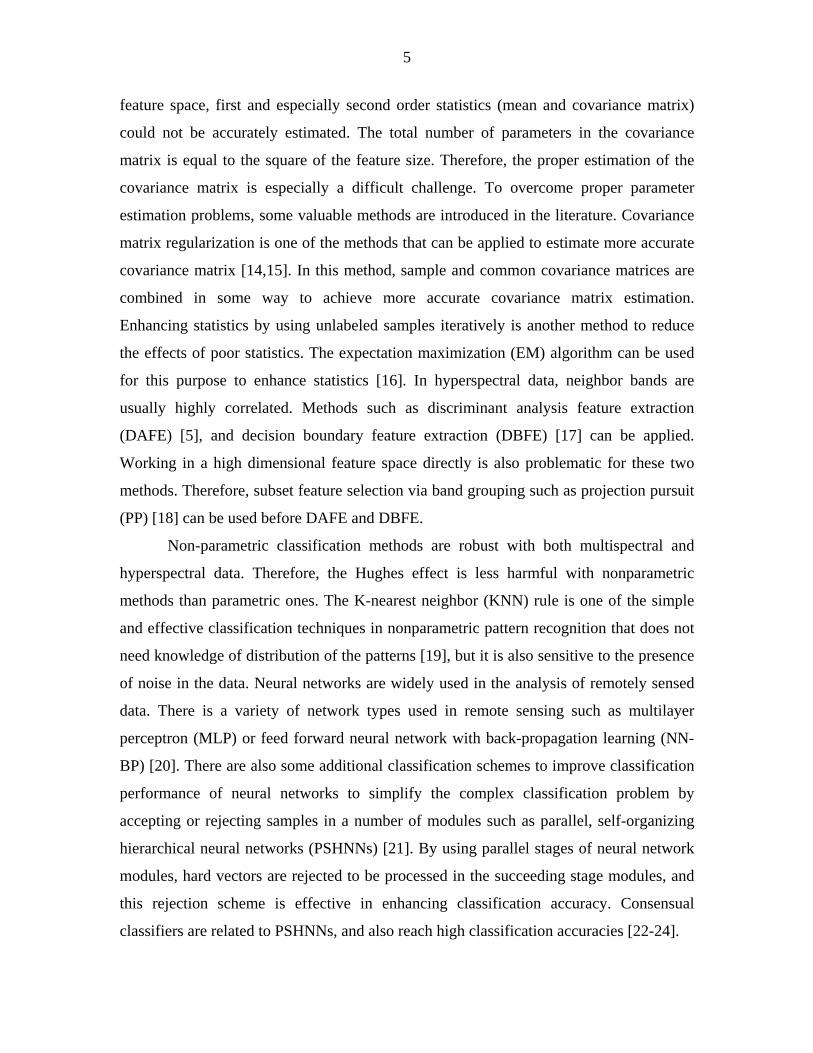
5

feature space, first and especially second order statistics (mean and covariance matrix)

could not be accurately estimated. The total number of parameters in the covariance

matrix is equal to the square of the feature size. Therefore, the proper estimation of the

covariance matrix is especially a difficult challenge. To overcome proper parameter

estimation problems, some valuable methods are introduced in the literature. Covariance

matrix regularization is one of the methods that can be applied to estimate more accurate

covariance matrix [14,15]. In this method, sample and common covariance matrices are

combined in some way to achieve more accurate covariance matrix estimation.

Enhancing statistics by using unlabeled samples iteratively is another method to reduce

the effects of poor statistics. The expectation maximization (EM) algorithm can be used

for this purpose to enhance statistics [16]. In hyperspectral data, neighbor bands are

usually highly correlated. Methods such as discriminant analysis feature extraction

(DAFE) [5], and decision boundary feature extraction (DBFE) [17] can be applied.

Working in a high dimensional feature space directly is also problematic for these two

methods. Therefore, subset feature selection via band grouping such as projection pursuit

(PP) [18] can be used before DAFE and DBFE.

Non-parametric classification methods are robust with both multispectral and

hyperspectral data. Therefore, the Hughes effect is less harmful with nonparametric

methods than parametric ones. The K-nearest neighbor (KNN) rule is one of the simple

and effective classification techniques in nonparametric pattern recognition that does not

need knowledge of distribution of the patterns [19], but it is also sensitive to the presence

of noise in the data. Neural networks are widely used in the analysis of remotely sensed

data. There is a variety of network types used in remote sensing such as multilayer

perceptron (MLP) or feed forward neural network with back-propagation learning (NN-

BP) [20]. There are also some additional classification schemes to improve classification

performance of neural networks to simplify the complex classification problem by

accepting or rejecting samples in a number of modules such as parallel, self-organizing

hierarchical neural networks (PSHNNs) [21]. By using parallel stages of neural network

modules, hard vectors are rejected to be processed in the succeeding stage modules, and

this rejection scheme is effective in enhancing classification accuracy. Consensual

classifiers are related to PSHNNs, and also reach high classification accuracies [22-24].

6

In recent years, kernel methods such as support vector machines (SVMs) have

demonstrated good performance in multispectral and hyperspectral data classification

[25-27]. Some of the drawbacks of SVMs are the necessity of choosing an appropriate

kernel function and time-intensive optimization. In addition, the assumptions made in the

presence of samples which are not linearly separable are not necessarily optimal. It is also

possible to use composite kernels [27] for remote sensing image classification to reach

higher classification accuracies.

In this paper, a new classification algorithm well suited for classification of

remote sensing images is developed with a new approach to detecting and adapting

border features with the training data. This approach is especially effective when the

information source has a limited amount of data samples, and the distribution of the data

is not necessarily Gaussian. Training samples closer to class borders are more prone to

generate misclassification, and therefore are significant features to be used to reduce

classification errors. The proposed classification algorithm searches for such error-

causing training samples in a special way, and adapts them to generate border features to

be used as labeled features for classification.

The BFDA algorithm can be considered in two parts. The first part of the

algorithm consists of defining initial border features using class centers and misclassified

training samples. With this approach, a manageable number of border features are

detected. The second part of the algorithm is the adaptation of the border features by

using a technique which has some similarity with the learning vector quantization (LVQ)

algorithm [28]. In this adaptation process, the border features are adaptively modified to

support proper distances between them and the class centers, and to increase the margins

between neighboring border features with different class labels. The class centers are also

adapted during this process. Subsequent classification is based on labeled border features

and class centers. With this approach, a proper number of features for each class is

generated by the algorithm.

The paper consists of four sections. The BFDA and consensual BFDA (C-BFDA)

are presented in Section II. The data sets used and the experimental results obtained with

them are presented in Section III. Conclusions and discussion of future research are

presented in Section IV.

7

II. BORDER FEATURE DETECTION AND ADAPTATION

Partitioning feature space by using some selected reference vectors from a

training set is a well-known approach in pattern recognition [29]. In general, there is an

optimal number of reference vectors which can be used. More number of reference

vectors above the optimal number may cause reduction of generalization performance. To

avoid performance reduction, additional efforts should be taken to discard redundant

reference vectors. An example of such a procedure is discussed in the grow and learn

algorithm (GAL) [29].

We propose a new approach to reference vector selection called border feature

detection. In developing such an approach, the selected reference vectors are required to

satisfy certain geometric considerations. For example, a major property of SVMs is to

optimize the margin between the hyperplanes characterizing different classes [9]. The

training vectors on the hyperplanes (in a separable problem) are called support vectors. In

the proposed algorithm, the same type of consideration leads to the positions of the

reference vectors selected from the training set to be adapted so that they better represent

the decision boundaries while the reference vectors from different classes are as far away

from each other as possible. These adapted reference vectors are called border features.

A. Border Feature Detection

The border feature detection algorithm is developed by considering the following

requirements:

1. Border features should be adapted so that they represent the decision boundaries as

well as possible.

2. The initial selection and adaptation procedure is desired to be automatic, with a

reasonable number of initial border features.

3. Every class should be represented with an appropriate number of border features to

properly represent the class.

In order to choose the initial border features, the class centers are used. A

particular class center is defined as the nearest vector to its class mean. Using class center

8

instead of class mean is a precaution for some classes which are spread in a concave form

in the feature space.

Assuming a labeled training dataset 1 2{( , ), ( , ), , ( , )}ny y y⋅ ⋅ ⋅1 2 nx x x where the

training samples are , 1,...,N i∈ =ix n , the class labels are {1, 2, , }iy m∈ ⋅ ⋅ ⋅ , is the

total number of training samples, and is the number of classes, the class means are

calculated as follows:

n

m

1 ,{ | , 1, , }1

niy i i mjn ji

= = = ⋅ ⋅ ⋅∑=

m x xi j j (1)

where is the total number of training samples for class i. The class center in ic for class i

is defined as follows:

{ }

( ) { }2

1

arg min,

(1 ), (1 ),

( , ) ( ) - ( ) ,N

i j jd

k

i m j n

m d x d y i=

⎧ ⎫=⎪ ⎪⎪ ⎪≤ ≤ ≤ ≤= ⎨ ⎬⎪ ⎪= − = =⎪ ⎪⎩ ⎭

∑

j

i k

j i j i j j

D

c x

D m x m x x

(2)

Let be a set of border features in the feature space. For t=0, is the set of initial

border features chosen as a combination of initial border feature sets :

tΒ 0Β

iB

(3) 0i

0

=i m≤ ≤

B∪Β

0B is chosen as the set of initial class centers. They can be written together with their

class labels as

{ }0 1 2 1 2( , ), ( , ), , ( , ) {( ), ( ), , ( )}m my y y y y y= ⋅ ⋅ ⋅ = ⋅ ⋅ ⋅B 1 2 m 1 2 mc c c b , b , b , . (4)

The number of members for the set is0B 0m m= . Additionally,

is chosen as a set of initial border features detected for class i as discussed next. Assume

that the total number of detected border features is for class i. In this assignment

procedure, is called the reference set for class i, and the number of members

for the reference set is . At the beginning of the detection procedure for every

class, ,and therefore, . During the detection process for class i=q,

, 1 i m= ⋅ ⋅ ⋅Bi

im

0= ∪R B Bi i

0 im m+

(t=0)=∅Bi 0t=0R ( ) = Bi

9

every member of the training samples belonging to class is randomly selected only

once as an input. Assume that

q

( , )k ky q=x is selected. Then, the Euclidean distances

calculated between this sample and the current reference set members are given by

0( , ) , 1...( )qj m m= − = +j k j k jD x b x b (5)

The winning border feature is chosen by

{ }arg min jw D= (6)

If the label of the winning border feature wb is w ky y q≠ = , then ( , )k ky q=x is

chosen as a new reference vector for class q and added to the reference vector set. This

can be written as (t) = (t -1) {( , )}ky q=∪R Ri=q i=q kx . This procedure is somewhat similar

to the ART1 algorithm [30]. The procedure for selecting border features is applied with

all the classes.

We define b as the total number of border features, and as the

number of detected border features for class i, with being the number of classes.

Then, the following is true:

, 1,...,im i m=

0 = m m

0 1

m m

ii i

b m m= =

= = + im∑ ∑ . (7)

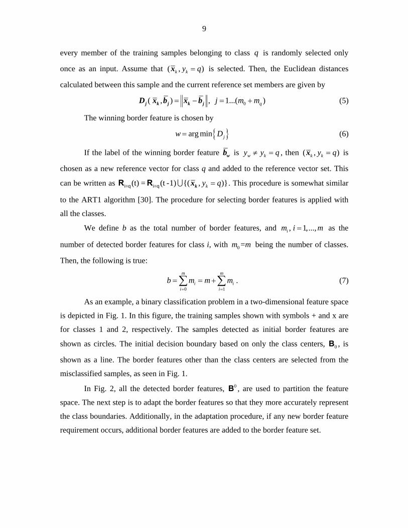
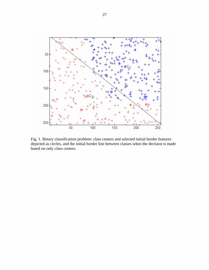
As an example, a binary classification problem in a two-dimensional feature space

is depicted in Fig. 1. In this figure, the training samples shown with symbols + and x are

for classes 1 and 2, respectively. The samples detected as initial border features are

shown as circles. The initial decision boundary based on only the class centers, , is

shown as a line. The border features other than the class centers are selected from the

misclassified samples, as seen in Fig. 1.

0B

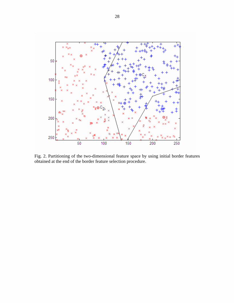
In Fig. 2, all the detected border features, , are used to partition the feature

space. The next step is to adapt the border features so that they more accurately represent

the class boundaries. Additionally, in the adaptation procedure, if any new border feature

requirement occurs, additional border features are added to the border feature set.

0Β

10

B. Adaptation Procedure

In the adaptation process, competitive learning principles are applied as follows:

The initial border features, are adaptively modified to support maximum distance

between the border features and their means, and to increase the margins between

neighboring border features with different class labels. The means of border features to

be used during adaptation are given by

0Β

1

1 ,{ | , 1, , }1

b

jji

y i i mm =

= = = ⋅+ ∑i j jm b b ⋅ ⋅ (8)

{ }01 2( , ), ( , ), ,( , ) my y y= ⋅ ⋅ ⋅M 1 2 mm m m (9)

The means of border features are not taken in to account in the final decision

process. Hence, at the end of the adaptation process, the means of border features are

redundant. During the adaptation process, they are used to decide whether new border

features should be generated. They are also adapted during learning due to the changes of

border features.

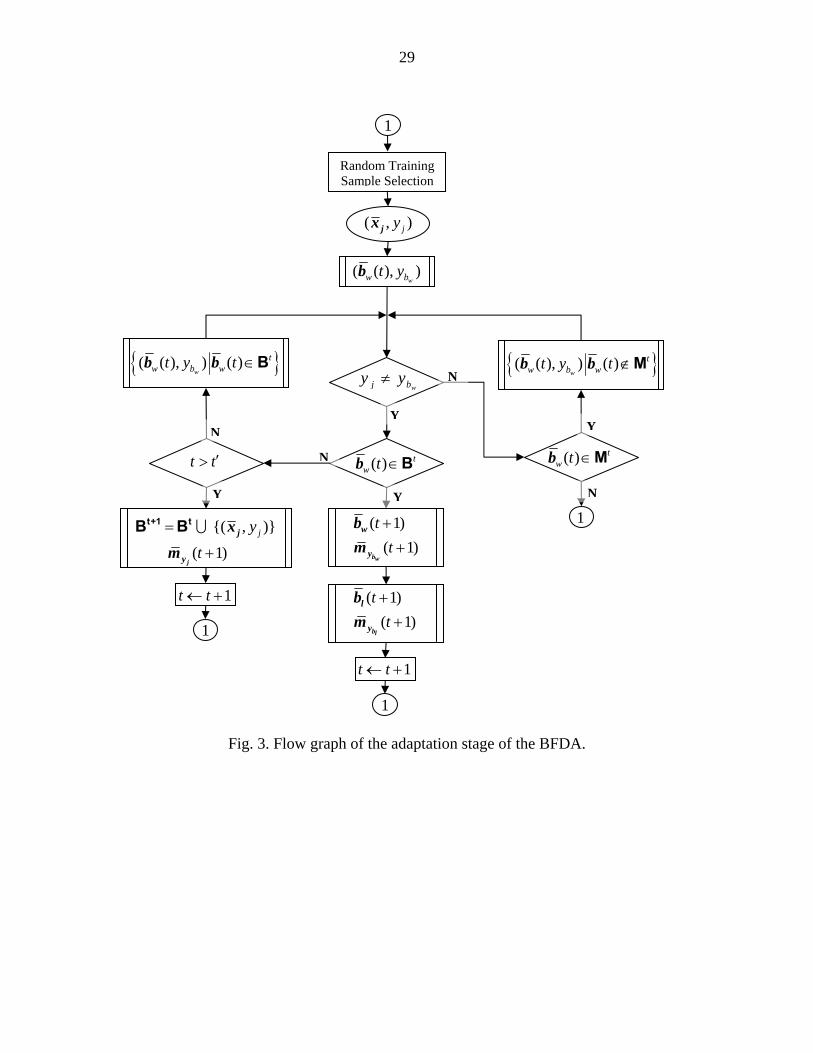
The strategy of adaptation can be explained as follows: a nearest border feature

( )twb which causes wrong decision should be farther away from the current training

sample. On the other hand, the nearest border feature ( )tlb with the correct class label

should be closer to the current training sample. The corresponding adaptation process

used has some similarity with the LVQ algorithm [28]. The adaptation procedure is

depicted as a flow graph in Fig. 3.

Let jx be one of the training samples with label jy . Assume that ( )w tb is the

nearest border feature to jx with label .If wby

wj by y≠ , then the adaptation is applied as

follows:

( 1) ( ) ( ) ( ( )) jt t t tη+ = − ⋅ −w w wb b x b (10)

( )( )( 1) ( ) ( ) ( ) b bw wy jt m t t t mη+ = ⋅ − ⋅ −

b bw wy y wm m x b y (11)

On the other hand, if ( )tlb is the nearest border feature to jx with label and lby

lj by y= ,

then

( 1) ( ) ( ) ( ( )) jt t t tη+ = + ⋅ −l l lb b x b (12)

11

( )( )( 1) ( ) ( ) ( ) bl ly jt m t t t mη+ = ⋅ + ⋅ −

b bl ly y lm m x bby (13)

where ( )tη is a descending function of time and is called the learning rate. A good choice

for it is given by

/0( ) tt e τη η −= (14)

During training, after a predefined number of iterations, t′ , the combination of

and are used as reference nodes to classify input training samples. If the nearest

node to a selected training sample

Mt tΒ

jx with label jy is one of the means of the border

features (t t′>wm ) with label and if wmy

wj my y≠ , then the wrongly classified training

sample jx is added as an additional border feature :

{( , )}, ( )jy t t′= >∪t+1 tΒ Β jx (15)

The corresponding mean vector is also adapted as follows:

( )( 1) ( ) ( ) ( ( ) 1)jy j yt m t t m t+ = ⋅ + +

j jy ym m xj

(16)

where is the number of border features belonging to class ( )jym t jy at iteration t.

Therefore is the number of border features in class ( 1)jym t + jy after the addition of the

new border feature.

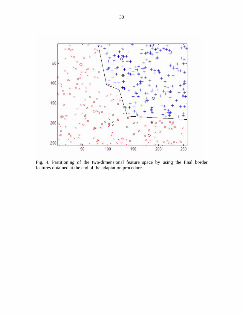
To illustrate the theory, the synthetic data result for the chosen binary

classification problem in the two-dimensional space is depicted in Fig. 4. After the

adaptation process, the final border features shown as circles and the final decision

boundary as combination of partial lines is observed in Fig. 4.

During testing with the testing dataset, classification is currently based on the

minimum distance rule with the border features determined at the end of the adaptation

procedure.

C. Consensus Strategy with Cross Validation

In supervised learning, the training process should be unbiased to reach more

accurate results in testing. In the BFDA, accuracy is related to the initialization of the

border features and the input ordering of the training samples. These dependencies make

the classifier a biased decision maker. Consensus strategy can be applied with cross

12

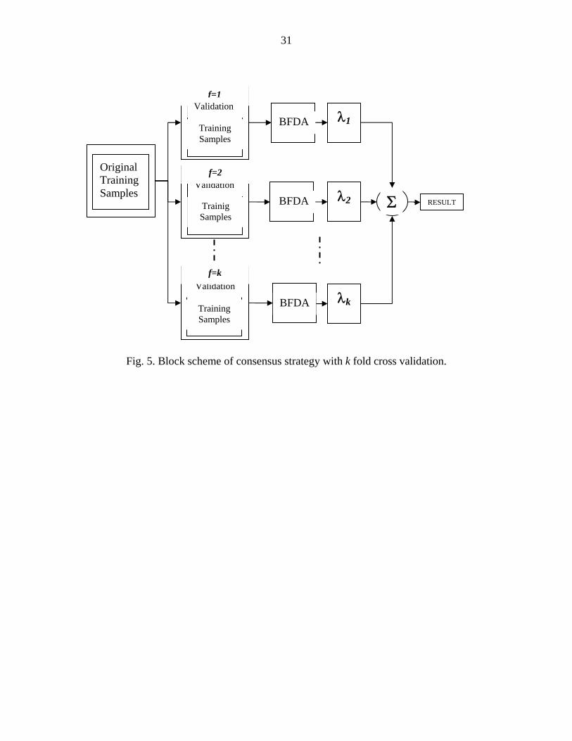
validation to reduce these dependencies. The cross validation fold number, f should be

chosen big enough with a limited number of training samples. The block scheme of

consensus strategy with k fold cross validation is depicted in Fig. 5.

There are a variety of consensual rules that can be applied to combine k individual

results to obtain improved classification. The reliability factor of the classification results

is depicted as a weight kλ for the kth BFDA classifier in Fig. 5. This reliability factor can

be specified by the consensual rule applied. For majority voting (MV) rule, weights can

be equally chosen, and the majority label is taken as the final label. It is also possible to

use a non-equal voting structure (Qualified Majority Voting, QMV) based on training

accuracies [31]. By using cross validation as a part of the consensual strategy, part of the

training samples are used for cross validation, and reliability factors can be assigned more

precisely based on validation. Once the reliability factors are determined, consensual

classification results can be obtained by applying a maximum rule with reliability factors.

Additionally, obtaining optimal reliability factors (weights, kλ ) can be done by least

squares analysis [12].

III. EXPERIMENTAL RESULTS

Reliable datasets well-known in the literature are more convenient to evaluate the

performance of the proposed BFDA algorithm than datasets which are not tested before.

Two well known data sets which are widely encountered in the literature were used in the

experiments for this purpose [32,33]. One additional data set from Turkey [34] was also

used to make proper comparison, and to show the robustness of the proposed algorithm.

As a consequence, three different data sets, one of them having four different

combinations of training samples and corresponding classes, were used in the

experiments to demonstrate a large number of results obtained with the BFDA. We were

able to show that the overall classification accuracies obtained with the BFDA are

satisfactory. Additionally, we were able to present rare class members are more

accurately classified than some other classification methods. Another goal of the

experiments was to show the Hughes effect [6] is less harmful with the BFDA than other

conventional statistical methods. This meant that the performance of the BFDA with a

13

limited number of training samples is generally higher than the performances of

conventional classifiers.

The performance of the BFDA was compared with other classification algorithms

including neural networks with back-propagation learning (NN-BP) [7], support vector

machines (SVMs) [25,26] and some statistical classification techniques such as maximum

likelihood (ML) and Fisher linear likelihood (FLL) [35]. The data analysis software called

Multispec [32] was used to perform the statistical classification methods. Linear SVM and

SVM with a radial basis kernel function were implemented in MATLAB using SVMlight

[36], and its MATLAB interface [37]. A one-against-one multiclassification scheme was

adopted in the experiments to compare SVMs performance to BFDA’s. Only spectral

features were taken into account in the comparison of the BFDA with other classification

techniques.

A. Choice of Parameters

How to choose the parameters for the BFDA is an important concern. Three

parameters need to be assigned. These parameters are the learning rate η, the time constant

τ and predefined number of iterations, t′ . For fast convergence, η=0.1 and τ=1000 were

found satisfactory. Faster training is suitable for relatively less complex classification

problems. For more complex classification problems, finer tuning may be necessary, and

η=0.2, τ=6750 can be chosen. Parameter selection for the BFDA has also some similarity

with the SOM [28]. Additionally, extra border feature requirements are controlled by

using a predefined number of iterations, t′ , during the adaptation process. This situation

occurs especially for complex classification problems. In the experiments, t = was

chosen. During the training process, a validation set can be used with a pocket algorithm

to avoid overfitting.

5000′

Determination of proper parameters is also an important concern for most other

classification algorithms such as the SVM classifiers. SVM is a binary classifier, and one-

against-one (OAO) strategy was used to generate multi-class SVM classifier in this study.

For one-against-one strategy, C and γ should be chosen for every binary class

combination. We assigned common parameters for each binary SVM classifier empirically

based on the training samples. High overall classification accuracies can be obtained by

14

using common parameter selection. Similar common parameter assignment was applied in

[25]. One drawback may occur with datasets which have unbalanced numbers of training

samples. In this situation, although high overall classification accuracy may be obtained,

accuracies of the rare classes may be lower than overall classification accuracy. It is

possible to use a multi class SVM classifier by reducing the classification to a single

optimization problem. This approach may also require fewer support vectors than a multi-

class classification approach based on combined use of many binary SVMs [38].

Neural network with back-propagation learning (NN-BP) was chosen in the

experiments as a well-known neural network classifier. 1 hidden layer with 15 neurons

was chosen as the network structure with learning rate equal to 0.01 and maximum

iteration number equal to 1000.

For the KNN classifier also used in the experiments, the choice of K is related to

the generalization performance of the classifier. Choosing a small number of K causes

reduction of generalization of the KNN classifier. It is also true that K=1 is the most

sensitive choice to noisy samples. Therefore K=5 was chosen in the experiments.

B. Description of the Datasets and the Experiments

Three different datasets were used in the experiments. The names of the

experiments are chosen the same as the names of the datasets, which are AVIRIS

(Airborne Visible/Infrared Imaging Spectrometer) Data [32], Satimage Data [33] and

Karacabey data [34].

B.1. AVIRIS Data Experiment

The AVIRIS image taken from the northwest Indiana’s Pine site in June 1992 [32]

was used in the experiments. This is a well known test image and has been often used for

validating hyperspectral image classification techniques [35,39]. Detailed comparisons

were made by using the AVIRIS data set in this paper. We used the whole scene

consisting of the full 145 x 145 pixels with two different class combinations, and two

different spectral band combinations. The training sample sets with 17 classes (pixels with

class labels of mixture type were considered for classification) and 9 classes (more

significant classes from the statistical viewpoint) were generated with different

15

combinations of 9 (to illustrate multispectral data classification performance) and 190

spectral bands (30 channels discarded from the original 220 spectral channels because of

atmospheric problems). 9 spectral bands used in datasets 1 and 3 were obtained by using

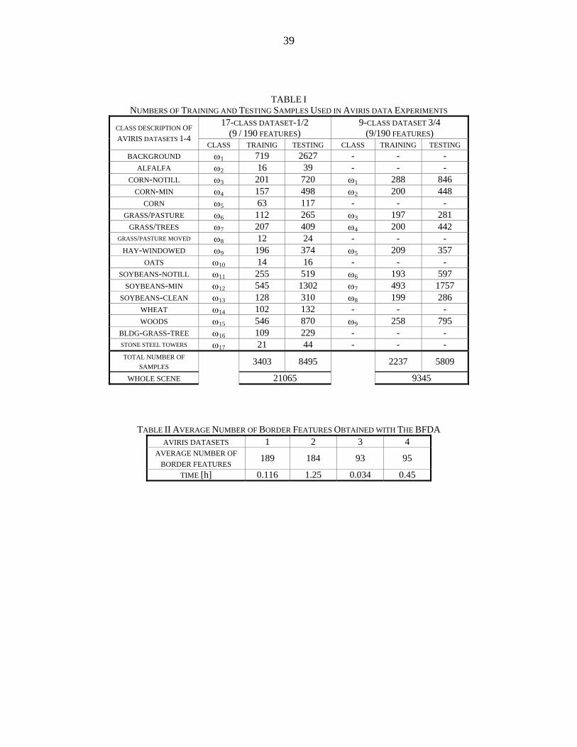
projection pursuit based on subset feature selection via band grouping. Table I shows the

number of training and testing samples for 17 and 9 class sets which were used in the

experiments. Datasets 1 and 2 contain background and building-grass-tree classes which

are of mixture type. Therefore, these two classification experiments involved more

complex classification problems than the other datasets. Additionally, datasets 1 and 2

have rare class members which have a limited number of training samples (alfalfa, oats,

stone steel towers, etc). Statistically meaningful classes were chosen for the datasets 3 and

4.

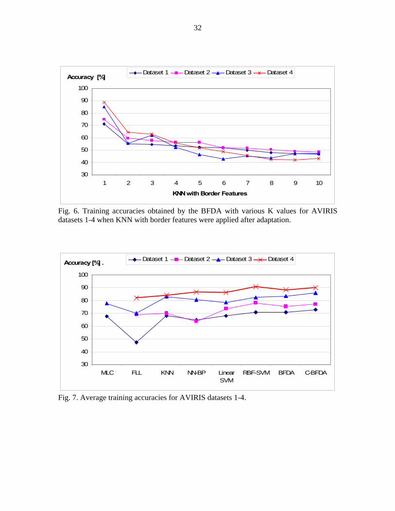
In the BFDA, classification is currently based on the minimum distance rule with

the finalized border features for the testing data. This rule can be thought of as a 1-

nearest neighbor (1-NN) with border features. The aim of the BFDA is to occupy the

feature space by using a minimum number of border features. Therefore, the nearest

border features typically have different class labels, causing K > 1 to yield worse results.

For example, the classification accuracies for dataset 1 are shown in Fig. 6 for different K

values. The highest accuracies were obtained with K=1 as expected.

Average testing accuracies obtained are shown in Fig. 7 for the AVIRIS data

experiments. The maximum likelihood classifier (MLC) results were obtained only for

datasets 1 and 3 because of the requirement of additional training samples to accurately

estimate the sample covariance matrix for every class. Higher number of training samples

is needed for proper sample covariance matrix estimation in high dimensional feature

space (datasets 2 and 4). Additionally, the Hughes effect is much more harmful for

quadratic classifiers.

The Fisher linear likelihood (FLL) algorithm was also used as an example of

statistical classifiers. The inverse of the common covariance matrix is used in the

discriminant function of the FLL. Therefore, all the classes are assumed to have the same

variance and correlation structure.

The results obtained with the K-Nearest Neighbor (KNN) were very satisfactory in

lower dimensional feature space (datasets 1 and 3). In the KNN algorithm, all the training

16

set members are used as reference vectors. Therefore, testing time takes more than other

conventional classification techniques.

For complex classification problems (datasets 1 and 2) we obtained relatively poor

classification results with the neural network based on back-propagation learning (NN-

BP). For statistically meaningful datasets, we obtained satisfactory results with the NN-BP

(datasets 3 and 4). Therefore, approximately equal number of training samples should be

selected to achieve better results with the NN-BP.

In general, the differences of the accuracies between datasets 2 and 1 and datasets

4 and 3 illustrate the robustness of the algorithms with respect to the Hughes effect (see

Fig. 7). Based on this consideration, the RBF-SVM, Consensual BFDA (C-BFDA), the

BFDA and the Linear SVM are observed to be the most robust algorithms with respect to

the Hughes effect. As observed in Fig. 7, these algorithms also produce case independent

results.

In low dimensional feature space, we obtained higher classification accuracies with

the BFDA and the C-BFDA. The performance of the BFDA in high dimensional feature

space was also satisfactory as seen in Fig. 7. In high dimensional feature space, we

obtained highest classification accuracies with the RBF-SVM and the C-BFDA. The

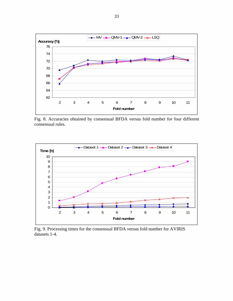
accuracies obtained with the C-BFDA versus fold number K are shown in Fig. 8 with four

different consensual rules for dataset 1. These rules are majority voting (MV), qualified

majority voting based on overall classification accuracies obtained by each validation set

(every fold) (QMV-1), qualified majority voting based on class by class accuracies

obtained by each validation set (QMV-2) and optimal weight selection based on least

squares analysis (LSE). Best accuracies were obtained for f=10 and MV rule for dataset 1.

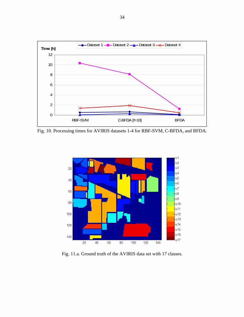
Processing time is also an important concern for our proposed consensual strategy

which is related to fold number (f). The total processing time for the C-BFDA versus fold

number f are shown in Fig. 9 for datasets 1-4. More complex classification problem

(dataset 2) needs much more time when we compare with other datasets. This is directly

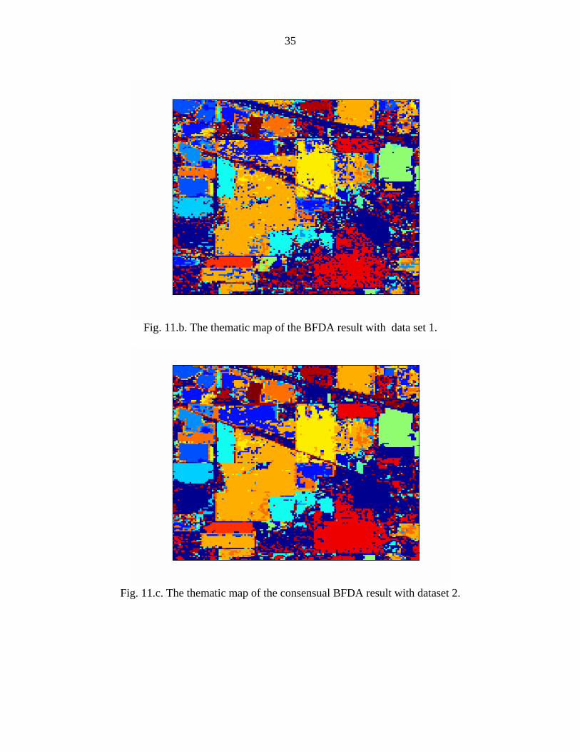
related to the number of classes and feature size. Total processing times are shown in Fig.

10 for RBF-SVM, BFDA and C-BFDA. It is shown that the RBF-SVM used more

processing time as compared to the C-BFDA and the BFDA. As observed in Fig. 10, the

processing time of the BFDA is reasonable.

17

The average number of border features used in the BFDA algorithm is shown in

Table II together with processing times for datasets 1-4. Border feature detection

procedure supports a proper number of border feature requirements dependent on the

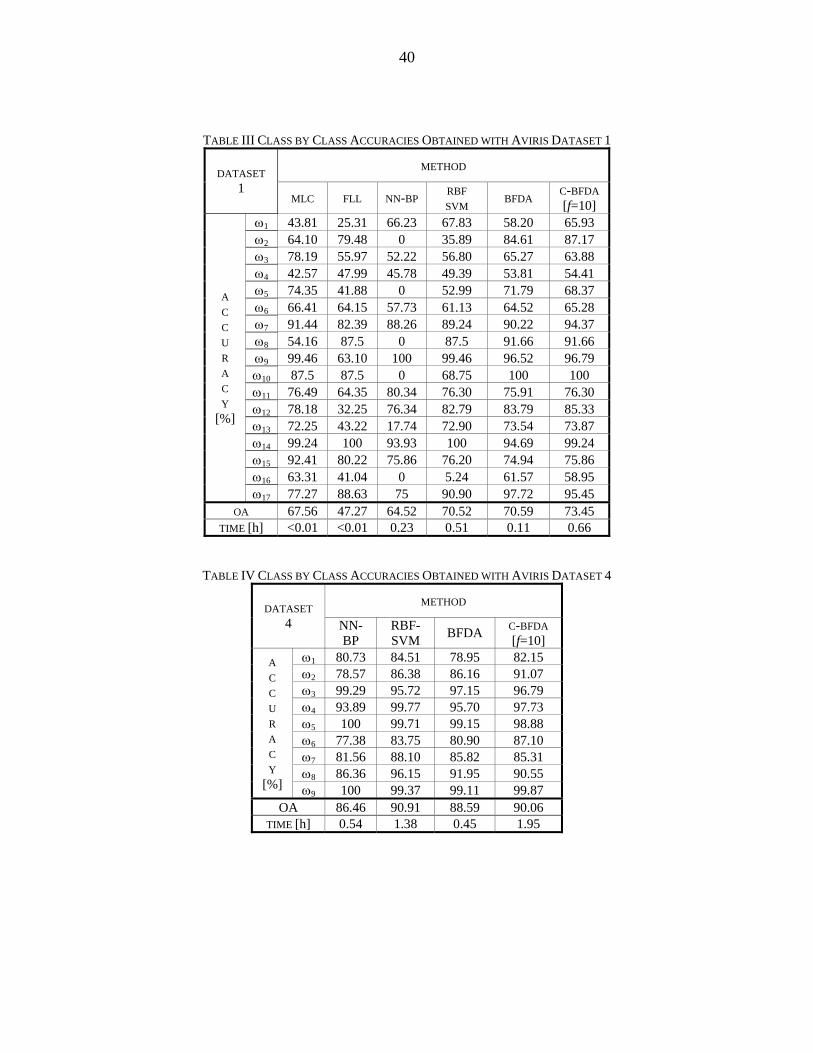
complexity of the problem. For detailed analysis, class by class accuracies are also given

for datasets 1 and 4 in Table III and Table IV, respectively.

The relatively low accuracy of class 1 (background class which is mixture type) in

dataset 1 reduced overall classification accuracy for the MLC as observed in Table III.

Reduction effects of the mixture type classes are much more harmful with the FLL in

dataset 1. We can conclude that the presence of the mixture type class members reduces

the overall classification accuracy with the statistical classifiers, as observed with dataset

1.

The neural network with back-propagation learning (NN-BP) is based on

minimizing the overall square error. As a result, the rare class members are not detected in

dataset 1 as expected. The performance of the NN-BP was satisfactory for dataset 4 which

has only statistically meaningful classes, as observed in Table IV. One interesting

observation was the very low accuracy of class 16 (building-grass-tree which is mixture

type rare class member) in dataset 1 with the RBF-SVM classifier as observed in Table

III. Common parameter assignment for each binary SVM classifier may have caused this

result.

With the BFDA and the C-BFDA, we obtained very satisfactory results for both

datasets 1 and 4, as observed in Tables III and IV. The BFDA reached high overall

classification accuracy while correctly classifying rare class members as observed in Table

III. Furthermore, the C-BFDA was used to enhance classification accuracy of the single

BFDA classifier by using cross validation in the consensual strategy with reasonable

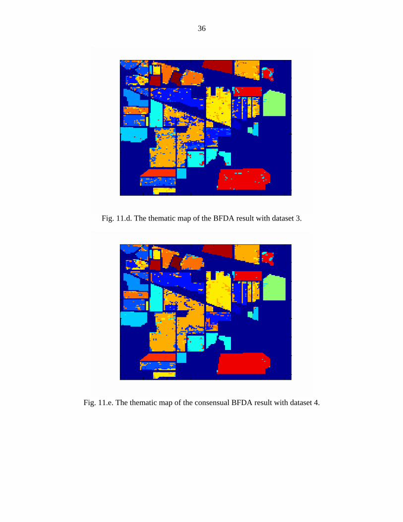
processing time, as observed in Tables III and IV. The thematic maps obtained with the

BFDA and the C- BFDA are depicted in Figures 11.b, and 11.c for datasets 1-2 and

Figures 11.d and 11.e for datasets 3-4, respectively.

B.2. Satimage Data Experiment

The satimage data set is a part of the Landsat MSS data and contains six different

classes. 4435 training samples and 2000 testing samples were obtained from the statlog

18

web site with their labels [33]. Training set contains statistical meaningful samples for

each class as shown in Table V. 4 spectral bands were used with one neighboring feature

extraction method to extract features. As a result, 4x9=36 features were assigned to a

pixel.

Highest accuracy in previous works with this data set was obtained with the SVM

[38]. In this experiment, the RBF-SVM classifier, the NN-BP and the MLC were used to

make comparisons with the BFDA and the C-BFDA. The aim of this experiment was to

demonstrate the robustness of the results obtained with the BFDA, and to illustrate the

performance of the BFDA on additional types of remotely sensed data in comparison

with other methods. The parameters of the BFDA were chosen as η=0.2, and τ=6750 for

learning rate and time constant respectively in this experiment. This parameter selection

makes slow convergence and fine tuning possible. The classification accuracy of the

RBF-SVM (C=16, γ=1) classifier with one-against-one strategy was reported as 91.3 %

for the satimage testing data set in reference [38]. In this experiment C=6 and γ=1.5 were

chosen by using a pattern search algorithm with a validation set. 15 neurons in one

hidden layer were chosen with the learning rate equal to 0.01 as network parameters for

the neural network with back-propagation learning. The activation function of the neural

network was chosen as the sigmoid function. In comparison, the testing results obtained

with the C-BFDA and the RBF-SVM were almost same and satisfactory for the satimage

data set as observed in Table V. Approximately 4 % less average accuracy were obtained

for the NN-BP when we compare the average of results obtained by the RBF-SVM, the

BFDA and the C-BFDA. Additionally less accurate result (27.48 %) was obtained for

class damp grey soil by the MLC. Therefore, the MLC were not sufficient to make

detailed class discrimination (for class damp grey soil) for this experiment. Obtained

accuracies for this problematic class were %54.04, %66.82, %67.29 and %68.72 by NN-

BP, RBF-SVM, BFDA and C-BFDA respectively. Therefore the best accurate results

were obtained by the BFDA and the C-BFDA for this specific class is obvious.

B.3. Karacabey Data Experiment

The Karacabey Data set is a Landsat 7 ETM+ image taken from northwest

Turkey, Karacabey region in Bursa in July 2000 [34]. Six visible infrared bands (Band 1-

19

5 & 7) having 30 m resolution were used as spectral features. Previous work was used as

auxiliary information for extraction of the ground reference data [34]. A color composite

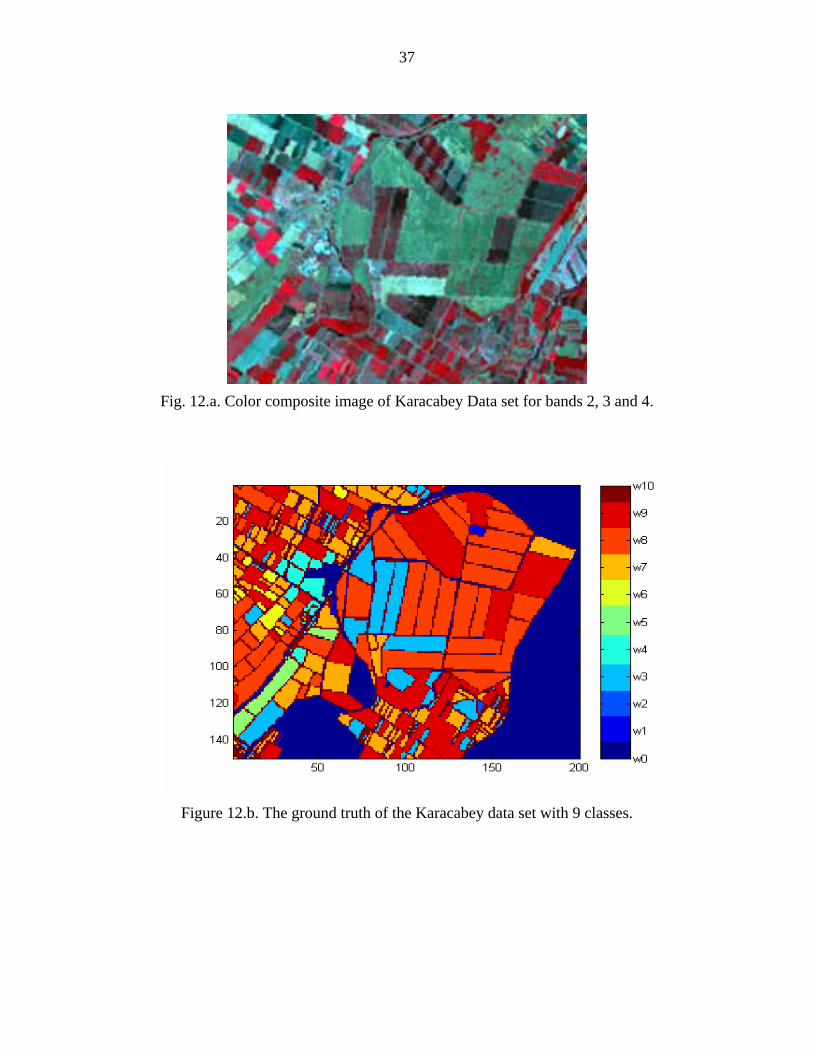
of the sub-image is shown in Fig. 12.a, and the ground truth map used in our experiments

is depicted in Fig. 12.b.

9 classes were utilized while background and parcel boundaries (depicted as w0

and w10 in the ground truth map, see Fig. 12.b) were discarded from evaluation.

Discarding of parcel boundaries supports selection of pure pixels. Therefore, pixels

which contain mixture spectral responses discarded in this experiment. Same selection

process was applied in reference [34]. However, there have been some advantages

reported in reference [8] related to selection of pixels which have mixture type spectral

responses especially for classifiers such as SVMs which are utilized training samples near

decision boundaries.

The description of the classes and the numbers of class samples used in the

experiment depicted in Table VI and the average training and testing accuracies as well

as the accuracies obtained with the whole scene are shown in Table VII. Balanced

numbers of training and testing samples were selected randomly; therefore obtained

results for testing and whole scene are shown same behavior. Our goal was to

demonstrate whether the BFDA is robust and performs well, in general. In this

experiment, we compared the BFDA with the SVM classifiers and the MLC.

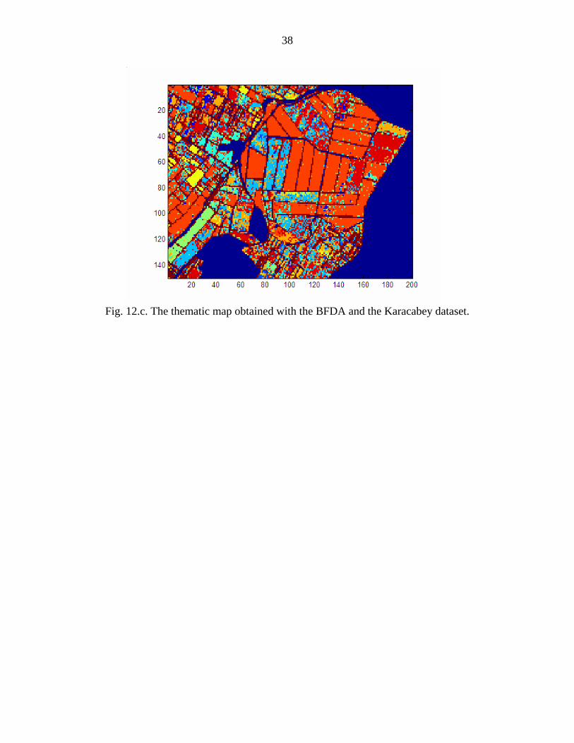
As we observe in Table VII, the results obtained with the BFDA and the C-BFDA

(67.41 % and 68.80 % respectively for whole scene) are satisfactory in comparison to

MLC (63.80 %). We obtained better result (%69.20 for whole scene) with RBF-SVM

classifier in this experiment. The average classification accuracies are less than 70 %.

Using only one multispectral data is not sufficient for discriminating detailed class types.

In the previous work [34], three different scenes acquired in approximately one month

period were used for classification. This indicates that multitemporal data classification

can be used to improve classification accuracy further. The thematic map of the BFDA

result for the Karacabey dataset is depicted in Fig. 12.c.

IV. CONCLUSIONS AND FUTURE WORK

In this study, we proposed a new algorithm for classification of remote sensing

images. The method first makes use of detected border features as part of an adaptation

20

process aimed at better describing the classes, and then uses minimum distance to border

feature rule for classification. The concept of border features proposed in this paper has

some similarity with support vectors in SVM classifiers. However, the procedure of the

initialization of border features, and subsequent adaptation process to find final border

features is completely different. The competitive learning principle is applied during the

adaptation procedure. In this sense, the adaptation algorithm used has some similarity

with the LVQ algorithm. The reason for this adaptation strategy is to satisfy the

maximum margin principle adaptively. It may be useful to mention some other

classification algorithms which have some similarity to the BFDA. The GAL algorithm

randomly chooses a subset of training samples to satisfy a predefined training accuracy

until a reaching predefined iteration number without any geometric consideration. The

border features chosen in the BFDA are different. The KNN algorithm uses the whole

training set as reference vectors. This makes the obtained results very sensitive to noise.

Another drawback of the KNN is processing time which is very high for classification of

large datasets. In the BFDA algorithm, a small number of border features are chosen.

The BFDA is a nonparametric classifier, robust against the Hughes effect, and

well-suited for remote sensing applications. In order to reach higher classification

accuracies C-BFDA which combines individual results of the BFDAs based on

consensual rule via cross validation was introduced. Additionally, appropriate safe

rejection schemes [21] can be applied to the BFDA to reach higher classification

accuracies. The BFDA algorithm utilizes training samples near decision boundaries.

Therefore using pixels which are mixed spectral responses can be increased the

performance of the classifier with the limited number of training samples which has been

reported in reference [8] for the SVM classifiers. Additionally in the spatial space, there

are also a variety of applications suitable for processing with the BFDA, such as target

detection, and contour specification. In conclusion, the BFDA can be applied in various

suitable applications in remote sensing, image processing, and other classification

applications.

21

ACKNOWLEDGMENT

The authors would like to thank GLCF (Global Land Cover Facility) for

providing Landsat 7 ETM+ data which is used as Karacabey data set in the experiment.

22

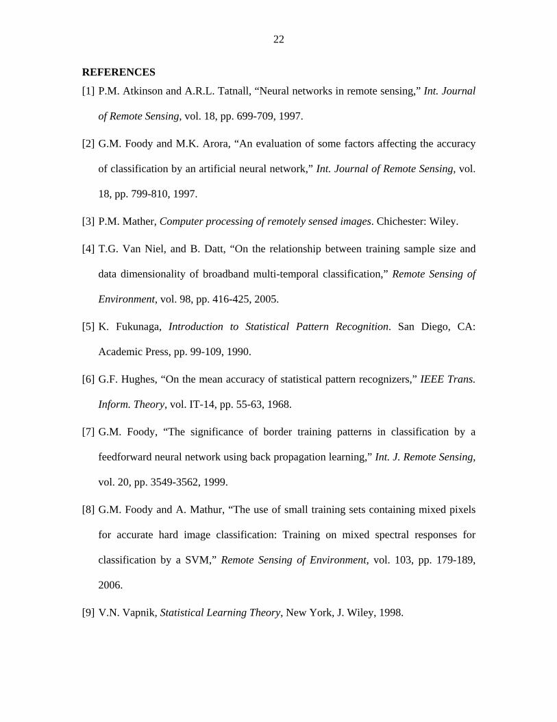
REFERENCES

[1] P.M. Atkinson and A.R.L. Tatnall, “Neural networks in remote sensing,” Int. Journal

of Remote Sensing, vol. 18, pp. 699-709, 1997.

[2] G.M. Foody and M.K. Arora, “An evaluation of some factors affecting the accuracy

of classification by an artificial neural network,” Int. Journal of Remote Sensing, vol.

18, pp. 799-810, 1997.

[3] P.M. Mather, Computer processing of remotely sensed images. Chichester: Wiley.

[4] T.G. Van Niel, and B. Datt, “On the relationship between training sample size and

data dimensionality of broadband multi-temporal classification,” Remote Sensing of

Environment, vol. 98, pp. 416-425, 2005.

[5] K. Fukunaga, Introduction to Statistical Pattern Recognition. San Diego, CA:

Academic Press, pp. 99-109, 1990.

[6] G.F. Hughes, “On the mean accuracy of statistical pattern recognizers,” IEEE Trans.

Inform. Theory, vol. IT-14, pp. 55-63, 1968.

[7] G.M. Foody, “The significance of border training patterns in classification by a

feedforward neural network using back propagation learning,” Int. J. Remote Sensing,

vol. 20, pp. 3549-3562, 1999.

[8] G.M. Foody and A. Mathur, “The use of small training sets containing mixed pixels

for accurate hard image classification: Training on mixed spectral responses for

classification by a SVM,” Remote Sensing of Environment, vol. 103, pp. 179-189,

2006.

[9] V.N. Vapnik, Statistical Learning Theory, New York, J. Wiley, 1998.

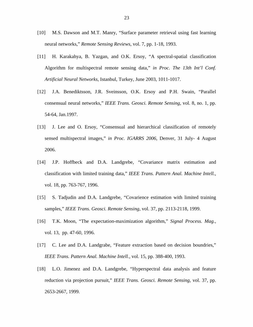
23

[10] M.S. Dawson and M.T. Manry, “Surface parameter retrieval using fast learning

neural networks,” Remote Sensing Reviews, vol. 7, pp. 1-18, 1993.

[11] H. Karakahya, B. Yazgan, and O.K. Ersoy, “A spectral-spatial classification

Algorithm for multispectral remote sensing data,” in Proc. The 13th Int’l Conf.

Artificial Neural Networks, Istanbul, Turkey, June 2003, 1011-1017.

[12] J.A. Benediktsson, J.R. Sveinsson, O.K. Ersoy and P.H. Swain, “Parallel

consensual neural networks,” IEEE Trans. Geosci. Remote Sensing, vol. 8, no. 1, pp.

54-64, Jan.1997.

[13] J. Lee and O. Ersoy, “Consensual and hierarchical classification of remotely

sensed multispectral images,” in Proc. IGARRS 2006, Denver, 31 July- 4 August

2006.

[14] J.P. Hoffbeck and D.A. Landgrebe, “Covariance matrix estimation and

classification with limited training data,” IEEE Trans. Pattern Anal. Machine Intell.,

vol. 18, pp. 763-767, 1996.

[15] S. Tadjudin and D.A. Landgrebe, “Covarience estimation with limited training

samples,” IEEE Trans. Geosci. Remote Sensing, vol. 37, pp. 2113-2118, 1999.

[16] T.K. Moon, “The expectation-maximization algorithm,” Signal Process. Mag.,

vol. 13, pp. 47-60, 1996.

[17] C. Lee and D.A. Landgrabe, “Feature extraction based on decision boundries,”

IEEE Trans. Pattern Anal. Machine Intell., vol. 15, pp. 388-400, 1993.

[18] L.O. Jimenez and D.A. Landgrebe, “Hyperspectral data analysis and feature

reduction via projection pursuit,” IEEE Trans. Geosci. Remote Sensing, vol. 37, pp.

2653-2667, 1999.

24

[19] T.M. Cover and P.E. Hart, “Nearest neighbor pattern classification,” IEEE Trans.

Information Theory, vol. 13, pp. 21-27, 1967.

[20] P.M. Atkinson and A.R.L. Tatnall, “Neural networks in remote sensing,” Int.

Journal of Remote Sensing, vol. 18, pp. 699-709, 1997.

[21] S. Cho, O.K. Ersoy, and M.R. Lehto, “Parallel, self-organizing, hierarchical

neural networks with competitive learning and safe rejection schemes,” IEEE Trans.

Circuits and Systems, vol. 40, no. 9, pp. 556-567, Sept. 1993.

[22] J.A. Benediktsson, J.R. Sveinsson and P.H. Swain, “Hybrid consensus theoretic

classification,” IEEE Trans. Geosci. Remote Sensing, vol. 35, no. 4, pp. 833-843, July

1997.

[23] J.A. Benediktsson and I. Kanellopoulos, “Classification of multisource and

hyperspectral data based on decision fusion,” IEEE Trans. Geosci. Remote Sensing,

vol. 37, no. 3, pp. 1367-1376, May 1999.

[24] Hoi-Ming Chee and O.K. Ersoy, A statistical self-organizing learning system for

remote sensing classification, IEEE Trans. Geosci. Remote Sensing, vol. 432, pp.

1890-1900, 2005.

[25] F. Melgani and L. Bruzzone, “Classification of hyperspectral remote sensing

images with support vector machines,” IEEE Trans. Geosci. Remote Sensing, vol. 42,

pp. 1778-1790, Aug. 2004.

[26] G.M. Foody and A. Mathur, “A relative evaluation of multiclass image

classification by support vector machines,” IEEE Trans. Geosci. Remote Sensing, vol.

42, pp. 1335-1343, 2004.

25

[27] G.C. Valls, L.G. Chova, J.M. Mari, J.V. Frances and J.C., Marivilla, “Composite

kernels for hyperspectral image classification,” IEEE Geosci. and Remote Sensing

Letters, vol. 3, pp. 93-97 2006.

[28] T. Kohonen,“The self-organizing map,” Proceedings of the IEEE, vol. 78, no. 9,

Sept. 1990.

[29] E. Alpaydin, “GAL: networks that grow when they learn and shrink when they

forget,” TR 91-032, International Computer Science Institute, Berkeley, CA, 1991.

[30] G.A. Carpenter and S. Grosberg, “A Massively parallel architecture for a self

organizing neural pattern recognition machine,” Computer Vision, Graphics, and

Image Processing, vol. 37, pp. 54-115, 1987.

[31] L.O. Jimenez, A.M. Morell and A. Creus, “Classification of hyperdimensional

data based featre and decision fusion approaches using projection pursuit, majority

voting, and neural networks,” IEEE Trans. Geosci. Remote Sensing, vol. 37, no. 3,

May 1999.

[32] D. Landgrebe and L. Biehl, Multispec and AVIRIS NW Indiana’s Indian Pines

1992 data set. [Online]. Available: http://www.ece.purdue.edu /~biehl

/MultiSpec/index.html

[33] Satimage data set : [Online]. Available: http://www.liacc.up.pt/ML/old/statlog/

datasets.html

[34] M. Arikan, “Parcel based crop mapping through multi-temporal masking

classification of Landsat 7 images in Karacabey, Turkey,” Proceedings of the ISPRS

Symposium, Istanbul International Archives of Photogrammetry. Remote Sensing and

Spatial Information Science, vol 34, 2004.

26

[35] D.A. Landgrebe, Signal Theory and Methods in Multispectral Remote Sensing.

New Jersey, USA: John Wiley & Sons, 2003.

[36] T. Joachims, Making large-Scale SVM Learning Practical. Advances in Kernel

Methods - Support Vector Learning, B. Schölkopf and C. Burges and A. Smola (ed.),

MIT-Press, 1999.

[37] A.Schwaighofer, MATLAB Interface to SVM light. Institute for Theoretical

Computer Science at Graz University of Technology. [Online]. Available:

http://www.cis.tugraz.at/igi/aschwaig/software.html.

[38] C. Hsu and C-J Lin, A comparison of methods for multiclass support vector

machines, IEEE Trans. Neural Networks, 13, 415-425 2002.

[39] P.K. Varshney and M.K. Arora, Advanced Image ProcessingTechniques for

Remotely Sensed Hyperspectral Data. New York, USA: Springer, 2004.

27

Fig. 1. Binary classification problem: class centers and selected initial border features depicted as circles, and the initial border line between classes when the decision is made based on only class centers.

28

Fig. 2. Partitioning of the two-dimensional feature space by using initial border features obtained at the end of the border feature selection procedure.

29

Random Training Sample Selection

wj by y≠

( ) tw t ∈b Β

( 1)( 1)

tt

++

bl

l

y

bm

1t t← +

1

t t′>

{( , )}

( 1)jy

t

=

+

∪t+1 tΒ Β

j

j

y

x

m

N

Y

{ }( ( ), ) ( )w

tw b wt y t ∈b b Β

( , )jyjx

( ) tw t ∈b M

1

{ }( ( ), ) ( )w

tw b wt y t ∉b b M

( ( ), )ww bt yb

( 1)( 1)

tt

++

bw

w

y

bm

1t t← +

1

1Y

NY

N

Y

N

Fig. 3. Flow graph of the adaptation stage of the BFDA.

30

Fig. 4. Partitioning of the two-dimensional feature space by using the final border features obtained at the end of the adaptation procedure.

31

Original Training Samples

Validation

Validation f=k

f=1 Validation

f=2

Training Samples

Trainig Samples

Training Samples

BFDA

Σ RESULT BFDA

BFDA

λ1

λ2

λk

Fig. 5. Block scheme of consensus strategy with k fold cross validation.

32

30

40

50

60

70

80

90

100

1 2 3 4 5 6 7 8 9 10

KNN with Border Features

Accuracy [%] Dataset 1 Dataset 2 Dataset 3 Dataset 4

Fig. 6. Training accuracies obtained by the BFDA with various K values for AVIRIS datasets 1-4 when KNN with border features were applied after adaptation.

30

40

50

60

70

80

90

100

MLC FLL KNN NN-BP LinearSVM

RBF-SVM BFDA C-BFDA

Accuracy [%] . Dataset 1 Dataset 2 Dataset 3 Dataset 4

Fig. 7. Average training accuracies for AVIRIS datasets 1-4.

33

62

64

66

68

70

72

74

76

2 3 4 5 6 7 8 9 10 11

Fold number

Accuracy [%]MV QMV-1 QMV-2 LSQ

Fig. 8. Accuracies obtained by consensual BFDA versus fold number for four different consensual rules.

0123456789

10

2 3 4 5 6 7 8 9 10 11

Fold number

Time [h]Dataset 1 Dataset 2 Dataset 3 Dataset 4

Fig. 9. Processing times for the consensual BFDA versus fold number for AVIRIS datasets 1-4.

34

0

2

4

6

8

10

12

RBF-SVM C-BFDA [f=10] BFDA

Time [h]Dataset 1 Dataset 2 Dataset 3 Dataset 4

Fig. 10. Processing times for AVIRIS datasets 1-4 for RBF-SVM, C-BFDA, and BFDA.

Fig. 11.a. Ground truth of the AVIRIS data set with 17 classes.

35

Fig. 11.b. The thematic map of the BFDA result with data set 1.

Fig. 11.c. The thematic map of the consensual BFDA result with dataset 2.

36

Fig. 11.d. The thematic map of the BFDA result with dataset 3.

Fig. 11.e. The thematic map of the consensual BFDA result with dataset 4.

37

Fig. 12.a. Color composite image of Karacabey Data set for bands 2, 3 and 4.

Figure 12.b. The ground truth of the Karacabey data set with 9 classes.

38

Fig. 12.c. The thematic map obtained with the BFDA and the Karacabey dataset.

39

TABLE I NUMBERS OF TRAINING AND TESTING SAMPLES USED IN AVIRIS DATA EXPERIMENTS

17-CLASS DATASET-1/2 (9 / 190 FEATURES)

9-CLASS DATASET 3/4 (9/190 FEATURES) CLASS DESCRIPTION OF

AVIRIS DATASETS 1-4 CLASS TRAINIG TESTING CLASS TRAINING TESTING

BACKGROUND ω1 719 2627 - - - ALFALFA ω2 16 39 - - -

CORN-NOTILL ω3 201 720 ω1 288 846 CORN-MIN ω4 157 498 ω2 200 448

CORN ω5 63 117 - - - GRASS/PASTURE ω6 112 265 ω3 197 281

GRASS/TREES ω7 207 409 ω4 200 442 GRASS/PASTURE MOVED ω8 12 24 - - -

HAY-WINDOWED ω9 196 374 ω5 209 357 OATS ω10 14 16 - - -

SOYBEANS-NOTILL ω11 255 519 ω6 193 597 SOYBEANS-MIN ω12 545 1302 ω7 493 1757

SOYBEANS-CLEAN ω13 128 310 ω8 199 286 WHEAT ω14 102 132 - - - WOODS ω15 546 870 ω9 258 795

BLDG-GRASS-TREE ω16 109 229 - - - STONE STEEL TOWERS ω17 21 44 - - - TOTAL NUMBER OF

SAMPLES 3403 8495 2237 5809

WHOLE SCENE 21065 9345

TABLE II AVERAGE NUMBER OF BORDER FEATURES OBTAINED WITH THE BFDA AVIRIS DATASETS 1 2 3 4

AVERAGE NUMBER OF BORDER FEATURES 189 184 93 95

TIME [h] 0.116 1.25 0.034 0.45

40

TABLE III CLASS BY CLASS ACCURACIES OBTAINED WITH AVIRIS DATASET 1

METHOD DATASET

1 MLC FLL NN-BP RBF

SVM BFDA C-BFDA [f=10]

ω1 43.81 25.31 66.23 67.83 58.20 65.93 ω2 64.10 79.48 0 35.89 84.61 87.17 ω3 78.19 55.97 52.22 56.80 65.27 63.88 ω4 42.57 47.99 45.78 49.39 53.81 54.41 ω5 74.35 41.88 0 52.99 71.79 68.37 ω6 66.41 64.15 57.73 61.13 64.52 65.28 ω7 91.44 82.39 88.26 89.24 90.22 94.37 ω8 54.16 87.5 0 87.5 91.66 91.66 ω9 99.46 63.10 100 99.46 96.52 96.79 ω10 87.5 87.5 0 68.75 100 100 ω11 76.49 64.35 80.34 76.30 75.91 76.30 ω12 78.18 32.25 76.34 82.79 83.79 85.33 ω13 72.25 43.22 17.74 72.90 73.54 73.87 ω14 99.24 100 93.93 100 94.69 99.24 ω15 92.41 80.22 75.86 76.20 74.94 75.86 ω16 63.31 41.04 0 5.24 61.57 58.95

A C C U R A C Y

[%]

ω17 77.27 88.63 75 90.90 97.72 95.45 OA 67.56 47.27 64.52 70.52 70.59 73.45

TIME [h] <0.01 <0.01 0.23 0.51 0.11 0.66

TABLE IV CLASS BY CLASS ACCURACIES OBTAINED WITH AVIRIS DATASET 4

METHOD DATASET 4 NN-

BP RBF-SVM BFDA C-BFDA

[f=10] ω1 80.73 84.51 78.95 82.15 ω2 78.57 86.38 86.16 91.07 ω3 99.29 95.72 97.15 96.79 ω4 93.89 99.77 95.70 97.73 ω5 100 99.71 99.15 98.88 ω6 77.38 83.75 80.90 87.10 ω7 81.56 88.10 85.82 85.31 ω8 86.36 96.15 91.95 90.55

A C C U R A C Y

[%] ω9 100 99.37 99.11 99.87 OA 86.46 90.91 88.59 90.06

TIME [h] 0.54 1.38 0.45 1.95

41

TABLE V CLASS BY CLASS ACCURACIES OBTAINED WITH SATIMAGE DATASET

TOTAL NUMBER OF SAMPLES METHOD SATIMAGE DATASET

CLASS DESCRIPTION TRAINING TESTING MLC NN-BP RBF-

SVM BFDA C-BFDA [f=10]

RED SOIL 1072 461 97.83 97.18 98.91 99.13 99.62 COTTON CROP 479 224 99.10 94.64 98.21 96.87 95.53

GREY SOIL 961 397 95.21 91.68 92.94 91.43 94.45 DAMP GREY SOIL 415 211 27.48 54.02 66.82 67.29 68.72

SOIL WITH STUBBLE 470 237 85.23 80.59 94.93 91.56 93.60 VERY DAMP GREY SOIL 1038 470

CLA

SS B

Y C

LASS

A

CC

UR

AC

Y [%

]

85.74 84.46 90.85 86.38 90.42 OA 85.7 86.3 91.9 90.1 92 TOTAL NUMBER OF

SAMPLES 4435 2000 AA 85.7 87.2 91.75 89.9 91.95

TABLE VI NUMBER OF SAMPLES FOR TRAINING, TESTING, AND WHOLE SCENE

KARACABEY DATASET

LABEL CLASS TRAINIG TESTING WHOLE SCENE

BARE SOIL ω1 10 10 66 WATERMELON ω2 10 10 27

PEPPER ω3 60 60 2110 PASTURE ω4 60 60 508 CLOVER ω5 60 60 442

SUGAR BEET ω6 60 60 300 TOMATO ω7 60 60 2694 RESIDU ω8 60 60 6846 CORN ω9 60 60 4752

TOTAL NUMBER OF SAMPLES 440 440 17737

TABLE VII AVERAGE CLASSIFICATION RESULTS WITH THE KARACABEY DATA SET ACCURACY [%]

METHOD TRAINING TESTING WHOLE

SCENE MLC 73.86 65.90 63.80

LINEER SVM 82.30 67.90 65.80 RBF-SVM 85.20 70.24 69.20

BFDA 87.24 68.80 67.41 C-BFDA [f=10] 88.40 70.02 68.80