Learning-Based Hyperspectral Imagery Compression through ...
Upload
khangminh22Category
view
2download
0
NTN
UN
orw
egia
n U
nive
rsity
of S
cien
ce a
nd T
echn
olog
yFa
culty
of I
nfor
mat
ion
Tech
nolo
gy a
nd E
lect
rical
Engi
neer
ing
Dep
artm
ent o
f Ele
ctro
nic
Syst
ems
Mas
ter’s
thes
is
Mohamed Ismail
HW/SW Co-design Implementation ofHyperspectral Image Classification Algorithm
Master’s thesis in Embedded Computing Systems
Supervisor: Milica Orlandic
June 2020


Mohamed Ismail
HW/SW Co-design Implementation ofHyperspectral Image Classification Algorithm
Master’s thesis in Embedded Computing SystemsSupervisor: Milica OrlandicJune 2020
Norwegian University of Science and TechnologyFaculty of Information Technology and Electrical EngineeringDepartment of Electronic Systems

Abstract
Hyperspectral Imager for Oceanographic Applications (HYPSO) mission is being de-veloped as a part of SmallSat laboratory at NTNU. The goal of the mission is to develop,launch, and operate a series of small satellites specially made for maritime observationand surveillance, e.g. monitoring of algae, plankton, oil spills, arctic ice etc. Satelliteswill be equipped with Zynq-7000 on-board processing system consisting of ARM®-basedprocessor with the hardware programmability of an FPGA.
In this thesis, on-board hyperspectral image classification on FPGA is explored. Basedon the hyperspectral data collected by the satellites, the detection of algae blooms orother material in the Norwegian sea can processed by classification. Classification aimsto distinguish and label material signatures on a given hyperspectral image. This thesispresents implementations of clustering-type unsupervised classification algorithms forhyperspectral images. Two algorithms are implemented in software; a novel segment-based clustering algorithm and a spectral clustering algorithm. The software implement-ations are implemented in MATLAB R2019a and Python 3.7.3, respectively. Expirementson the algorithms are carried on 8 different publicly available hyperspectral scenes withground truth data and results are compared with a state-of-the-art segment-based clus-tering method using NMI and Purity evaluation scores. Results of the software experi-ments are further analysed prior to FPGA implementation.
Based on the software analysis, spectral clustering algorithm is implemented as anovel hardware-software partitioned system on Xilinx Zynq-7000 development plat-form. The hardware-software co-design is implemented to gain the most efficiency com-pared to the standalone software solution. FPGA VHDL modules for graph constructionare developed and synthesized using Xilinx Vivado Design Suite 2019.1 and HDL Coder™
R2020a from MathWorks. Eigenvalue and eigenvector decomposition is implementedusing Vivado HLS 2019.1 and synthesized using Xilinx Vivado tool. This implement-ation illustrates productivity benefits of a C-based development flow using high-levelsynthesis (HLS) optimization methods. Resource utilization, performance, and classific-ation scores are reported for the HW/SW co-design of spectral clustering algorithm.
iii


Preface
This master’s thesis is the final part of my European Master degree in Embedded Com-puting Systems (EMECS). The thesis work was conducted at the Norwegian Universityof Science and Technology (NTNU) within a SmallSat project (HYPSO) and is a con-tinuation of the work done in a specialization project at NTNU. Hyperspectral imageclassification on FPGAs is a challenging topic and represents a very promising area ofresearch. This thesis allowed me to both acquire and enrich my knowledge and skills byexploring a wide spectrum of topics and tools involved in hyperspectral image classsi-fication. Moreover, as a student, I find it always wonderful and exciting to learn newtopics, and even though it has been a challenging learning experience, it has also beena rewarding and gratifying experience.
First of all, I would to like express my thanks, appreciation, and gratefulness to mysupervisor Milica Orlandic, for guiding me through this work, for always being availablefor my questions and discussions, for enlightening me to possible research dimensionsin my work, and for emotionally and academically supporting me through the events ofthe 2020 coronavirus global pandemic.
Finally, a special thanks to my family and friends for being a very solid supportsystem, a positive company, and for ensuring I am physically and psychologically wellthrough these months and weeks.
Mohamed IsmailJune 24, 2020.
v


Contents
Abstract . . . . . . . . . . . . . . . . . . . . . . . . . . . . . . . . . . . . . . . . . . . . . . iiiPreface . . . . . . . . . . . . . . . . . . . . . . . . . . . . . . . . . . . . . . . . . . . . . . . vContents . . . . . . . . . . . . . . . . . . . . . . . . . . . . . . . . . . . . . . . . . . . . . . viiFigures . . . . . . . . . . . . . . . . . . . . . . . . . . . . . . . . . . . . . . . . . . . . . . . ixTables . . . . . . . . . . . . . . . . . . . . . . . . . . . . . . . . . . . . . . . . . . . . . . . xiiiCode Listings . . . . . . . . . . . . . . . . . . . . . . . . . . . . . . . . . . . . . . . . . . . xv1 Introduction . . . . . . . . . . . . . . . . . . . . . . . . . . . . . . . . . . . . . . . . . 1
1.1 Motivation . . . . . . . . . . . . . . . . . . . . . . . . . . . . . . . . . . . . . . . 11.2 HSI Classification in the context of HYPSO mission . . . . . . . . . . . . . . 21.3 HYPSO mission payload . . . . . . . . . . . . . . . . . . . . . . . . . . . . . . . 31.4 Main Contributions . . . . . . . . . . . . . . . . . . . . . . . . . . . . . . . . . . 41.5 Structure of the Thesis . . . . . . . . . . . . . . . . . . . . . . . . . . . . . . . . 5
2 Background . . . . . . . . . . . . . . . . . . . . . . . . . . . . . . . . . . . . . . . . . 72.1 Hyperspectral Data Representation . . . . . . . . . . . . . . . . . . . . . . . . 72.2 HSI Classifcation Algorithms . . . . . . . . . . . . . . . . . . . . . . . . . . . . 9
2.2.1 Convolution Neural Networks . . . . . . . . . . . . . . . . . . . . . . . 92.2.2 Clustering Classification Algorithms . . . . . . . . . . . . . . . . . . . 10
2.3 State-of-the-art HSI Classification Algorithms . . . . . . . . . . . . . . . . . . 112.3.1 Supervised vs. Unsupervised Learning Methods . . . . . . . . . . . . 122.3.2 Segment-based Clustering . . . . . . . . . . . . . . . . . . . . . . . . . 132.3.3 Method Choice . . . . . . . . . . . . . . . . . . . . . . . . . . . . . . . . 14
2.4 Binary Partition Trees and HSI . . . . . . . . . . . . . . . . . . . . . . . . . . . 142.4.1 Pre-segmentation using Watershed Method . . . . . . . . . . . . . . . 152.4.2 BPT Building . . . . . . . . . . . . . . . . . . . . . . . . . . . . . . . . . 162.4.3 BPT Pruning . . . . . . . . . . . . . . . . . . . . . . . . . . . . . . . . . . 18
2.5 Filtering Algorithm . . . . . . . . . . . . . . . . . . . . . . . . . . . . . . . . . . 192.6 Spectral Clustering . . . . . . . . . . . . . . . . . . . . . . . . . . . . . . . . . . 21
2.6.1 Building the Similarity Graph . . . . . . . . . . . . . . . . . . . . . . . 212.6.2 Finding an Optimal Partition . . . . . . . . . . . . . . . . . . . . . . . . 212.6.3 Eigenvalue and Eigenvector Decomposition . . . . . . . . . . . . . . 262.6.4 Spectral Clustering Example . . . . . . . . . . . . . . . . . . . . . . . . 292.6.5 Nyström Extension . . . . . . . . . . . . . . . . . . . . . . . . . . . . . . 32
2.7 Overview of Zynq-7000 Functional Blocks . . . . . . . . . . . . . . . . . . . . 362.7.1 DSP blocks on Zynq . . . . . . . . . . . . . . . . . . . . . . . . . . . . . 372.7.2 AXI Protocols . . . . . . . . . . . . . . . . . . . . . . . . . . . . . . . . . 382.7.3 AXI DMA . . . . . . . . . . . . . . . . . . . . . . . . . . . . . . . . . . . . 40
vii
viii
2.7.4 Block RAM . . . . . . . . . . . . . . . . . . . . . . . . . . . . . . . . . . . 402.8 Vivado HLS . . . . . . . . . . . . . . . . . . . . . . . . . . . . . . . . . . . . . . . 42
3 Software Implementation . . . . . . . . . . . . . . . . . . . . . . . . . . . . . . . . 433.1 Segment-based Clustering using BPT . . . . . . . . . . . . . . . . . . . . . . . 43
3.1.1 Pre-Segmentation . . . . . . . . . . . . . . . . . . . . . . . . . . . . . . 443.1.2 BPT Building . . . . . . . . . . . . . . . . . . . . . . . . . . . . . . . . . 453.1.3 BPT Pruning . . . . . . . . . . . . . . . . . . . . . . . . . . . . . . . . . . 503.1.4 K-means Clustering . . . . . . . . . . . . . . . . . . . . . . . . . . . . . 51
3.2 Fast Spectral Clustering . . . . . . . . . . . . . . . . . . . . . . . . . . . . . . . 524 Software Results . . . . . . . . . . . . . . . . . . . . . . . . . . . . . . . . . . . . . . 55
4.1 Software Results for CLUS-BPT and FSC . . . . . . . . . . . . . . . . . . . . . 554.2 Experimental Datasets . . . . . . . . . . . . . . . . . . . . . . . . . . . . . . . . 554.3 Evaluation Metrics . . . . . . . . . . . . . . . . . . . . . . . . . . . . . . . . . . 59
4.3.1 Parameter Settings . . . . . . . . . . . . . . . . . . . . . . . . . . . . . . 594.4 Results and Comparisons . . . . . . . . . . . . . . . . . . . . . . . . . . . . . . 60
4.4.1 Effect of Number of Clusters . . . . . . . . . . . . . . . . . . . . . . . . 604.4.2 Computational Time . . . . . . . . . . . . . . . . . . . . . . . . . . . . . 64
4.5 Algorithm Choice . . . . . . . . . . . . . . . . . . . . . . . . . . . . . . . . . . . 665 HW/SW Co-design Implementation . . . . . . . . . . . . . . . . . . . . . . . . . . 67
5.1 Overall System Structure (HW/SW) . . . . . . . . . . . . . . . . . . . . . . . . 675.2 BRAM for Input and Processing Logic . . . . . . . . . . . . . . . . . . . . . . . 695.3 Similarity Graph Construction . . . . . . . . . . . . . . . . . . . . . . . . . . . 70
5.3.1 Sampling . . . . . . . . . . . . . . . . . . . . . . . . . . . . . . . . . . . . 705.3.2 Graph Construction . . . . . . . . . . . . . . . . . . . . . . . . . . . . . 71
5.4 Eigenvalue and Eigenvector Decomposition . . . . . . . . . . . . . . . . . . . 755.5 Spectral Embedding and K-means Clustering . . . . . . . . . . . . . . . . . . 81
6 HW/SW Co-design Results . . . . . . . . . . . . . . . . . . . . . . . . . . . . . . . . 856.1 Performance Analysis . . . . . . . . . . . . . . . . . . . . . . . . . . . . . . . . . 856.2 Resource Utilization . . . . . . . . . . . . . . . . . . . . . . . . . . . . . . . . . 866.3 Clustering Performance Analysis . . . . . . . . . . . . . . . . . . . . . . . . . . 88
7 Conclusion . . . . . . . . . . . . . . . . . . . . . . . . . . . . . . . . . . . . . . . . . . 937.1 Future Work . . . . . . . . . . . . . . . . . . . . . . . . . . . . . . . . . . . . . . 94
Bibliography . . . . . . . . . . . . . . . . . . . . . . . . . . . . . . . . . . . . . . . . . . . 95A Dimensionality Reduction . . . . . . . . . . . . . . . . . . . . . . . . . . . . . . . . 99B Gauss Jordan Elimination . . . . . . . . . . . . . . . . . . . . . . . . . . . . . . . . 101C Using HW/SW Co-design Implementation on Zynq Platform . . . . . . . . . . 103
C.1 Create Project . . . . . . . . . . . . . . . . . . . . . . . . . . . . . . . . . . . . . 103C.2 Synthesis and Simulation . . . . . . . . . . . . . . . . . . . . . . . . . . . . . . 103C.3 Post-synthesis and Implementation . . . . . . . . . . . . . . . . . . . . . . . . 106C.4 Xilinx SDK . . . . . . . . . . . . . . . . . . . . . . . . . . . . . . . . . . . . . . . 106
Figures
1.1 The Autonomous Ocean Sampling Network (AOSN) [3]. . . . . . . . . . . . 3
2.1 Illustration of a hyperspectral image [9]. . . . . . . . . . . . . . . . . . . . . . 72.2 Spectral signatures of different materials [9]. . . . . . . . . . . . . . . . . . 82.3 Hyperspectral Image BIP Storage Format. . . . . . . . . . . . . . . . . . . . . 82.4 A cartoon drawing of a biological neuron (left) and its mathematical
model (right) [10]. . . . . . . . . . . . . . . . . . . . . . . . . . . . . . . . . . . 92.5 K-means algorithm 2D example. . . . . . . . . . . . . . . . . . . . . . . . . . . 112.6 Flowchart of PCMNN. Dashed lines indicates that the local band selection
approach is incorporated within these operations [18]. . . . . . . . . . . . . 132.7 Example of hierarchical region-based representation using BPT [9]. . . . . 152.8 Topographic representation of a 2D mountain image [23]. . . . . . . . . . . 162.9 BPT construction using a region merging algorithm [9]. . . . . . . . . . . . 172.10 A grid representing the set of spectra for a region R containing M pixels
and modelled into one column of spectra. . . . . . . . . . . . . . . . . . . . . 172.11 Region-based pruning of the Binary Partition Tree using PR = 3 . . . . . . 182.12 Candidate z is pruned because C lies entirely on one side of the bisecting
hyperplane H [8]. . . . . . . . . . . . . . . . . . . . . . . . . . . . . . . . . . . . 192.13 A case where minimum cut gives a bad partition [32]. . . . . . . . . . . . . 222.14 Similarity graph corresponding to matrix W . . . . . . . . . . . . . . . . . . . 302.15 Spectral embedding example. . . . . . . . . . . . . . . . . . . . . . . . . . . . 322.16 Architectural Overview of Zynq-7000 [40]. . . . . . . . . . . . . . . . . . . . 372.17 Basic DSP48E1 Slice Functionality [41]. . . . . . . . . . . . . . . . . . . . . . 382.18 Block diagram of AXI interconnects connecting the processor and DMA
(in PS) to AXI DMA and a processing logic block (in PL). . . . . . . . . . . . 392.19 AXI4-Lite interface [42]. . . . . . . . . . . . . . . . . . . . . . . . . . . . . . . . 392.20 AXI4-Stream Interface. . . . . . . . . . . . . . . . . . . . . . . . . . . . . . . . . 402.21 Vector storage using BRAM. . . . . . . . . . . . . . . . . . . . . . . . . . . . . . 412.22 Vivado HLS Design Flow [46]. . . . . . . . . . . . . . . . . . . . . . . . . . . . 41
3.1 Flowchart of CLUS-BPT. . . . . . . . . . . . . . . . . . . . . . . . . . . . . . . . 433.2 Overall software modules hierarchy. . . . . . . . . . . . . . . . . . . . . . . . . 443.3 Example operations of dilation and erosion on a hyperspectral image. . . . 453.4 A tree node data structure. . . . . . . . . . . . . . . . . . . . . . . . . . . . . . 463.5 Variation of final segmentation maps for PaviaU image. . . . . . . . . . . . . 513.6 PCA and segmentation map embedding example. . . . . . . . . . . . . . . . 52
ix
x
3.7 Flowchart of FSC. . . . . . . . . . . . . . . . . . . . . . . . . . . . . . . . . . . . 52
4.1 Salinas scene ground truth map and labels reference. Salinas-A is high-lighted with a red box [47] . . . . . . . . . . . . . . . . . . . . . . . . . . . . . 56
4.2 Pavia Center scene ground truth map with labels reference [47] . . . . . . 564.3 Pavia University scene ground truth map with labels reference [47] . . . . 574.4 Indian Pines ground truth map and labels reference [47] . . . . . . . . . . . 574.5 Samson scene ground truth map and labels reference [47] . . . . . . . . . . 584.6 Jasper Ridge ground truth map and labels reference [47] . . . . . . . . . . 584.7 Urban dataset scene ground truth map and labels reference [47] . . . . . . 584.8 Average NMI values (10 runs) versus the number of regions (PR) for (a)
PaviaC and PaviaU, (b) Salinas and Indian Pines, (c) Jasper Ridge andUrban, and (d) Salinas-A and Samson. . . . . . . . . . . . . . . . . . . . . . . 61
4.9 NMI values obtained at different number of clusters for the proposedmethod. . . . . . . . . . . . . . . . . . . . . . . . . . . . . . . . . . . . . . . . . . 62
4.10 NMI values obtained at different number of clusters for the proposedmethod, for Salinas and Indian Pines images. . . . . . . . . . . . . . . . . . . 62
4.11 HSI ground truth and results. . . . . . . . . . . . . . . . . . . . . . . . . . . . . 634.12 HSI ground truth and results. . . . . . . . . . . . . . . . . . . . . . . . . . . . . 644.13 Computational time measured at different number of regions PR for the
proposed method. . . . . . . . . . . . . . . . . . . . . . . . . . . . . . . . . . . . 65
5.1 PS and PL Partitions in the Zynq-7000 HW/SW co-design. . . . . . . . . . . 675.2 Block diagram of BRAM module with register file. . . . . . . . . . . . . . . . 695.3 16-bit LFSR. . . . . . . . . . . . . . . . . . . . . . . . . . . . . . . . . . . . . . . 705.4 Implemented RTL design for graph A calculation. . . . . . . . . . . . . . . . 725.5 Implemented state machine for matrix A calculation. . . . . . . . . . . . . . 725.6 HLS SVD block design. . . . . . . . . . . . . . . . . . . . . . . . . . . . . . . . . 765.7 y pointer array points to the rows of E. . . . . . . . . . . . . . . . . . . . . . 82
6.1 Resource utilization as a function of varying number of spectral bands forBRAM module. . . . . . . . . . . . . . . . . . . . . . . . . . . . . . . . . . . . . . 87
6.2 Resource utilization as a function of varying number of spectral bands forProcessing Logic modules. . . . . . . . . . . . . . . . . . . . . . . . . . . . . . . 88
6.3 Cluster maps obtained from (a) FSC [12], (b) proposed CLUS-BPT, (c)proposed HW/SW, (d) ground reference image, and (e) ground referencecolor codes of classes for Urban image. . . . . . . . . . . . . . . . . . . . . . . 90
6.4 Cluster maps obtained from (a) FSC [12], (b) proposed CLUS-BPT, (c)proposed HW/SW, (d) ground reference image, and (e) ground referencecolor codes of classes for Jasper Ridge image. . . . . . . . . . . . . . . . . . . 90
6.5 Cluster maps obtained from (a) FSC [12], (b) proposed CLUS-BPT, (c)proposed HW/SW, (d) ground reference image, and (e) ground referencecolor codes of classes for Samson image. . . . . . . . . . . . . . . . . . . . . . 91
6.6 Cluster maps obtained from (a) FSC [12], (b) proposed CLUS-BPT, (c)proposed HW/SW, (d) ground reference image, and (e) ground referencecolor codes of classes for Salinas-A image. . . . . . . . . . . . . . . . . . . . . 91

Figures xi
C.1 Synthesis block diagram of HW/SW solution. . . . . . . . . . . . . . . . . . . 104C.2 Graph construction simulation waveform . . . . . . . . . . . . . . . . . . . . 105C.3 SDK - change project settings. . . . . . . . . . . . . . . . . . . . . . . . . . . . 106

Tables
2.1 Vivado HLS optimization directives [46]. . . . . . . . . . . . . . . . . . . . . 42
3.1 User defined parameters. . . . . . . . . . . . . . . . . . . . . . . . . . . . . . . 44
4.1 Best purity and NMI values obtained by PCMNN, FSC, and CLUS-BPT forSalinas and PaviaU images. . . . . . . . . . . . . . . . . . . . . . . . . . . . . . 61
4.2 Best purity and NMI values obtained by FSC and CLUS-BPT for the restof the images. . . . . . . . . . . . . . . . . . . . . . . . . . . . . . . . . . . . . . 62
4.3 Computational time for FSC and CLUS-BPT obtained for the best purityand NMI results for all datasets. . . . . . . . . . . . . . . . . . . . . . . . . . . 65
5.1 Generic parameters and example values for HW/SW codesign. . . . . . . . 695.2 AXI-lite register file description. . . . . . . . . . . . . . . . . . . . . . . . . . . 705.3 SVD Implementation Controls. . . . . . . . . . . . . . . . . . . . . . . . . . . . 75
6.1 Performance comparison for HW/SW codesign solution. . . . . . . . . . . . 856.2 Maximum frequency for HW/SW codesign solution modules. . . . . . . . . 866.3 Post-Synthesis resource utilization report. . . . . . . . . . . . . . . . . . . . . 876.4 Best purity and NMI scores obtained by HW/SW co-design proposed method,
FSC SW, and CLUS-BPT SW for images. . . . . . . . . . . . . . . . . . . . . . 89
xiii

Code Listings
3.1 Initialize node structures . . . . . . . . . . . . . . . . . . . . . . . . . . . . . . 473.2 Update node structures - Step 1. . . . . . . . . . . . . . . . . . . . . . . . . . . 483.3 Update node structures - Steps 2, 3, & 4. . . . . . . . . . . . . . . . . . . . . . 483.4 Final step in buildBPT. . . . . . . . . . . . . . . . . . . . . . . . . . . . . . . . . 493.5 BPT Pruning. . . . . . . . . . . . . . . . . . . . . . . . . . . . . . . . . . . . . . . 503.6 Python code in LATEX document . . . . . . . . . . . . . . . . . . . . . . . . . . . 535.1 HLS SVD C code. . . . . . . . . . . . . . . . . . . . . . . . . . . . . . . . . . . . 765.2 HLS SVD built-in function. . . . . . . . . . . . . . . . . . . . . . . . . . . . . . 775.3 svd2x2 function. . . . . . . . . . . . . . . . . . . . . . . . . . . . . . . . . . . . 785.4 SVD top function continued 1. . . . . . . . . . . . . . . . . . . . . . . . . . . . 795.5 Spectral Embedding in Zynq PS. . . . . . . . . . . . . . . . . . . . . . . . . . . 815.6 K-means Clustering function call. . . . . . . . . . . . . . . . . . . . . . . . . . 825.7 K-means Clustering function. . . . . . . . . . . . . . . . . . . . . . . . . . . . . 82B.1 Gauss Jordan implemented in C. . . . . . . . . . . . . . . . . . . . . . . . . . . 102
xv

Chapter 1
Introduction
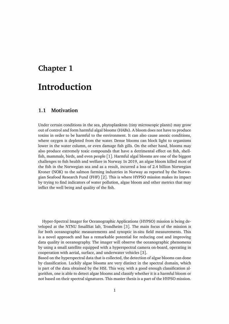
1.1 Motivation
Under certain conditions in the sea, phytoplankton (tiny microscopic plants) may growout of control and form harmful algal blooms (HABs). A bloom does not have to producetoxins in order to be harmful to the environment. It can also cause anoxic conditions,where oxygen is depleted from the water. Dense blooms can block light to organismslower in the water column, or even damage fish gills. On the other hand, blooms mayalso produce extremely toxic compounds that have a detrimental effect on fish, shell-fish, mammals, birds, and even people [1]. Harmful algal blooms are one of the biggestchallenges to fish health and welfare in Norway. In 2019, an algae bloom killed most ofthe fish in the Norwegian sea and as a result, incurred a loss of 2.4 billion NorwegianKroner (NOK) to the salmon farming industries in Norway as reported by the Norwe-gian Seafood Research Fund (FHF) [2]. This is where HYPSO mission makes its impactby trying to find indicators of water pollution, algae bloom and other metrics that mayinflict the well being and quality of the fish.
Hyper-Spectral Imager for Oceanographic Applications (HYPSO) mission is being de-veloped at the NTNU SmallSat lab, Trondheim [3]. The main focus of the mission isfor both oceanographic measurements and synoptic in-situ field measurements. Thisis a novel approach and has a remarkable potential for reducing cost and improvingdata quality in oceanography. The imager will observe the oceanographic phenomenaby using a small satellite equipped with a hyperspectral camera on-board, operating incooperation with aerial, surface, and underwater vehicles [3].Based on the hyperspectral data that is collected, the detection of algae blooms can doneby classification. Luckily algae blooms are very distinct in the spectral domain, whichis part of the data obtained by the HSI. This way, with a good enough classification al-gorithm, one is able to detect algae blooms and classify whether it is a harmful bloom ornot based on their spectral signatures. This master thesis is a part of the HYPSO mission.
1
2 1.2 HSI Classification in the context of HYPSO mission
1.2 HSI Classification in the context of HYPSO mission
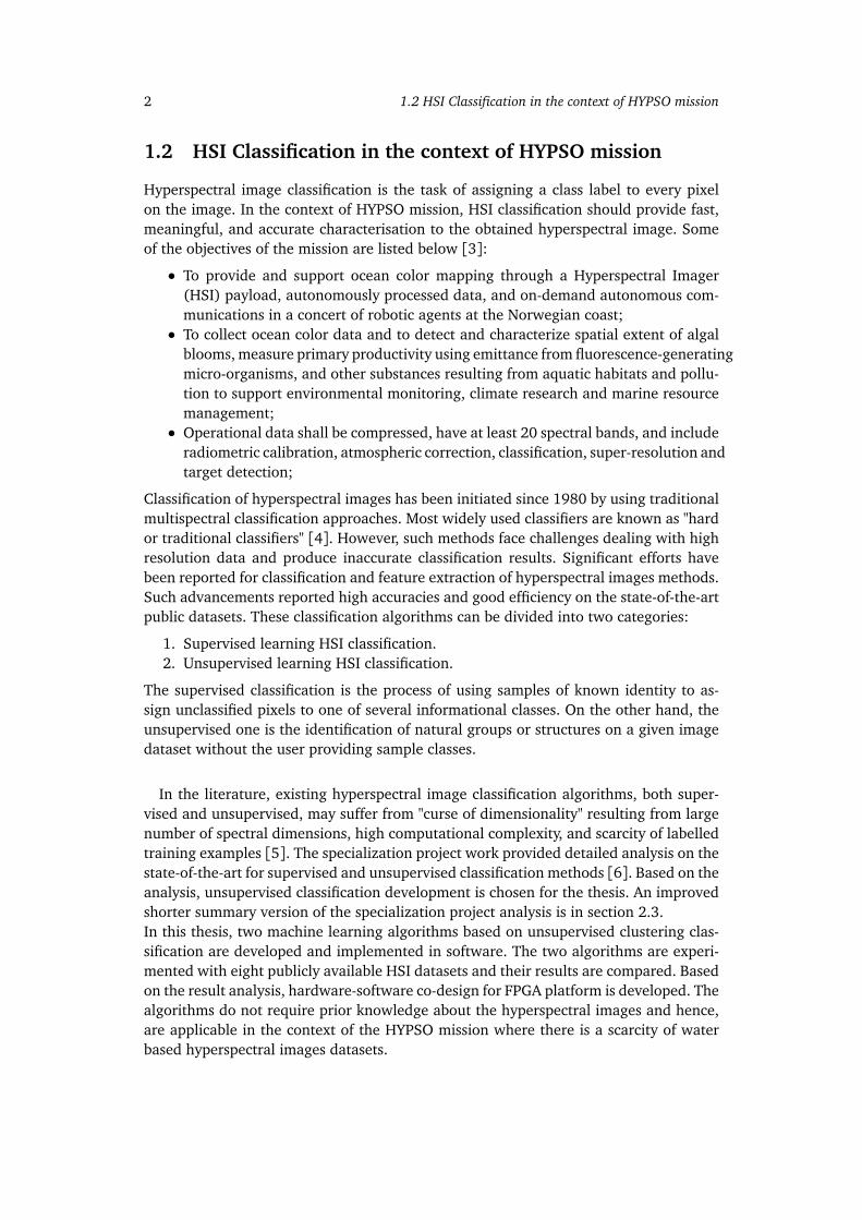
Hyperspectral image classification is the task of assigning a class label to every pixelon the image. In the context of HYPSO mission, HSI classification should provide fast,meaningful, and accurate characterisation to the obtained hyperspectral image. Someof the objectives of the mission are listed below [3]:
• To provide and support ocean color mapping through a Hyperspectral Imager(HSI) payload, autonomously processed data, and on-demand autonomous com-munications in a concert of robotic agents at the Norwegian coast;
• To collect ocean color data and to detect and characterize spatial extent of algalblooms, measure primary productivity using emittance from fluorescence-generatingmicro-organisms, and other substances resulting from aquatic habitats and pollu-tion to support environmental monitoring, climate research and marine resourcemanagement;
• Operational data shall be compressed, have at least 20 spectral bands, and includeradiometric calibration, atmospheric correction, classification, super-resolution andtarget detection;
Classification of hyperspectral images has been initiated since 1980 by using traditionalmultispectral classification approaches. Most widely used classifiers are known as "hardor traditional classifiers" [4]. However, such methods face challenges dealing with highresolution data and produce inaccurate classification results. Significant efforts havebeen reported for classification and feature extraction of hyperspectral images methods.Such advancements reported high accuracies and good efficiency on the state-of-the-artpublic datasets. These classification algorithms can be divided into two categories:
1. Supervised learning HSI classification.2. Unsupervised learning HSI classification.
The supervised classification is the process of using samples of known identity to as-sign unclassified pixels to one of several informational classes. On the other hand, theunsupervised one is the identification of natural groups or structures on a given imagedataset without the user providing sample classes.
In the literature, existing hyperspectral image classification algorithms, both super-vised and unsupervised, may suffer from "curse of dimensionality" resulting from largenumber of spectral dimensions, high computational complexity, and scarcity of labelledtraining examples [5]. The specialization project work provided detailed analysis on thestate-of-the-art for supervised and unsupervised classification methods [6]. Based on theanalysis, unsupervised classification development is chosen for the thesis. An improvedshorter summary version of the specialization project analysis is in section 2.3.In this thesis, two machine learning algorithms based on unsupervised clustering clas-sification are developed and implemented in software. The two algorithms are experi-mented with eight publicly available HSI datasets and their results are compared. Basedon the result analysis, hardware-software co-design for FPGA platform is developed. Thealgorithms do not require prior knowledge about the hyperspectral images and hence,are applicable in the context of the HYPSO mission where there is a scarcity of waterbased hyperspectral images datasets.
Chapter 1: Introduction 3
1.3 HYPSO mission payload
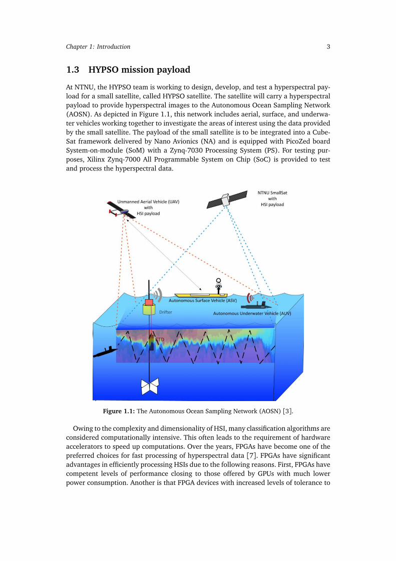
At NTNU, the HYPSO team is working to design, develop, and test a hyperspectral pay-load for a small satellite, called HYPSO satellite. The satellite will carry a hyperspectralpayload to provide hyperspectral images to the Autonomous Ocean Sampling Network(AOSN). As depicted in Figure 1.1, this network includes aerial, surface, and underwa-ter vehicles working together to investigate the areas of interest using the data providedby the small satellite. The payload of the small satellite is to be integrated into a Cube-Sat framework delivered by Nano Avionics (NA) and is equipped with PicoZed boardSystem-on-module (SoM) with a Zynq-7030 Processing System (PS). For testing pur-poses, Xilinx Zynq-7000 All Programmable System on Chip (SoC) is provided to testand process the hyperspectral data.
Figure 1.1: The Autonomous Ocean Sampling Network (AOSN) [3].
Owing to the complexity and dimensionality of HSI, many classification algorithms areconsidered computationally intensive. This often leads to the requirement of hardwareaccelerators to speed up computations. Over the years, FPGAs have become one of thepreferred choices for fast processing of hyperspectral data [7]. FPGAs have significantadvantages in efficiently processing HSIs due to the following reasons. First, FPGAs havecompetent levels of performance closing to those offered by GPUs with much lowerpower consumption. Another is that FPGA devices with increased levels of tolerance to
4 1.4 Main Contributions
ionizing radiation, making it suitable for space and are widely used as the solution foronboard processing at Earth observation satellites. In addition, FPGAs have the inherentability to change their functionality through partial or full reconfiguration, hence, opensthe possibility to select algorithms from a ground station [7].
The provided Xilinx Zynq-7000 SoC contains an ARM Cortex-A9 processor along withFPGA programmable logic and offers high performance ports to connect ARM processingsystem and FPGA programmable logic. This is very desirable for hardware and softwarecodesigned implementations. By deciding which elements will be performed by the pro-grammable logic, and which elements will run on the ARM Cortex-A9, the computationsystem is partitioned leading to the accelerated execution of hyperspectral processingalgorithms including classification algorithms.
1.4 Main Contributions
The specialization project [6] recommended the fulfillment of the following tasks in themaster thesis:
• Incorporation of methods like segmentation before classification (segment-basedclassification) for initially partitioning the hyperspectral image spatially. The pro-posed approach in the specialization project partitioned the regions by dividingthe HSI image into k regions iteratively by going through the whole image; whichis considered simple partitioning.
• Development of a two-level filtering algorithm before/during k-means clustering.• Change tree structure. The kd-trees discussed in the project represent strict rect-
angular partitions of the image which is very useful for plotted data points butmay not be suitable for hyperspectral images.
• Incorporation of dimensionality reduction methods including principal componentanalysis (PCA).
These tasks were approached in this thesis by development of two proposed solutions.The first one is a segment-based clustering where a full segmentation method basedon Binary Partition Trees (BPT) processes the HSI data before filtering k-means cluster-ing classification is applied. This framework represents a further development and en-hancement to the method presented in the specialization project [6], making it a novelframework in literature. The second one is an adaptation of a near-real time clusteringmethod for unsupervised HSI classification based on spectral clustering.Both frameworks are developed in software and are experimented on eight differentHSI datasets, including both land-cover and water-based datasets. Furthermore, exper-imental results are compared to state-of-the-art clustering methods. According to theanalysis of the experiments and the implementation of the methods, a novel HW/SWco-design solution is developed for the chosen method: spectral clustering.
To the best of the author’s knowledge, the HW/SW implementation in this work isa novel implementation for spectral clustering type methods on FPGA platforms. Con-sequently, a novel method for hyperspectral image clustering classification on FPGAs. Inliterature, the only clustering implementation for hyperspectral images on FPGAs has

Chapter 1: Introduction 5
been developed by [8] and is based solely on k-means clustering.In addition, this thesis proposes a new segment-clustering software framework for hyper-spectral images based on a three-stage scheme: (i) pre-segmentation, (ii) segmentation,and (iii) PCA and k-means clustering.
1.5 Structure of the Thesis
This section describes the organization of the rest of this thesis.Chapter 2 discusses the background information necessary for development of
the two HSI classification methods, for both software and hardware implementation. Inaddition, brief overview of Zynq-7000 platform is provided, with a short discussion onthe state-of-the-art HSI classification algorithms.
Chapter 3 presents the software implementation of both methods.Chapter 4 provides the experimental details including parameter settings. It also
analyzes the results obtained by the experiments and accordingly, the bases of choosinga suitable algorithm for HW/SW implementation.
Chapter 5 discusses the HW/SW co-design implementation of the spectral cluster-ing method.
Chapter 6 shows the synthesis results and metrics of the final design includinghardware performance, resource utilization, and classification performance.
Chapter 7 concludes the work with discussion and some remarks.Appendix consists of extra background information as well as guidlines for HW/SW
co-design setup and use.

Chapter 2
Background
2.1 Hyperspectral Data Representation
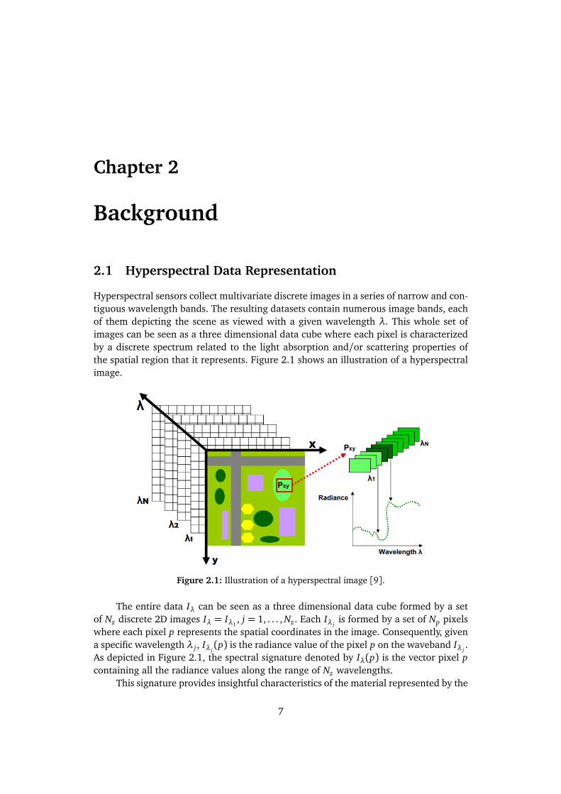
Hyperspectral sensors collect multivariate discrete images in a series of narrow and con-tiguous wavelength bands. The resulting datasets contain numerous image bands, eachof them depicting the scene as viewed with a given wavelength λ. This whole set ofimages can be seen as a three dimensional data cube where each pixel is characterizedby a discrete spectrum related to the light absorption and/or scattering properties ofthe spatial region that it represents. Figure 2.1 shows an illustration of a hyperspectralimage.
Figure 2.1: Illustration of a hyperspectral image [9].
The entire data Iλ can be seen as a three dimensional data cube formed by a setof Nz discrete 2D images Iλ = Iλ1
, j = 1, . . . , Nz . Each Iλ jis formed by a set of Np pixels
where each pixel p represents the spatial coordinates in the image. Consequently, givena specific wavelength λ j , Iλ j
(p) is the radiance value of the pixel p on the waveband Iλ j.
As depicted in Figure 2.1, the spectral signature denoted by Iλ(p) is the vector pixel pcontaining all the radiance values along the range of Nz wavelengths.
This signature provides insightful characteristics of the material represented by the
7

8 2.1 Hyperspectral Data Representation
pixel as shown for some materials in Figure 2.2.
Figure 2.2: Spectral signatures of different materials [9].
The spectral space is important because it contains much more information aboutthe surface of target materials than what can be perceived by the human eye. The spa-tial space is also important because it describes the spatial variations and correlationin the image and this information is essential to interpret objects in natural scenes. Hy-perspectral image classification methods highly desired goals include automatic featureextraction using either one or both data information (spectral and spatial), in order todistinguish different materials for a meaningful application.
In this work, the HSI image for the input logic is organized such that all spectralcomponents of one pixel are written in subsequent locations, followed by another pixelin a frame. Next row is formed for the next frame captured by the imager. Hence, bands1 to 3 are written for pixel 1 which is part of frame 1, followed by components of pixel2, and so on. This organization scheme is called band interleaved by pixel (BIP) formatand is used throughout this work. An illustration is presented in Figure 2.3.
Figure 2.3: Hyperspectral Image BIP Storage Format.

Chapter 2: Background 9
2.2 HSI Classifcation Algorithms
As introduced in section 1.2, HSI classification algorithms can be categorized into su-pervised methods and unsupervised methods. Due to the noises and redundancy amongspectral bands, many feature extraction, band selection, and dimension reduction tech-niques have been used for HSI classification in the past years. Supervised methods arepopularly known to go through these techniques and follow it by training and labeling.The first common step among supervised methods consists of transforming the image toa feature image to reduce the data dimensionality and improve the data interpretability.This processing phase is optional and comprises techniques such as principal compon-ent analysis. In the training phase, a set of training samples in the image is selected tocharacterize each class. Training samples train the classifier to identify the classes andare used to determine the criteria for the assignment of a class label to each pixel in theimage.
2.2.1 Convolution Neural Networks
Convolution Neural Networks (CNNs) are the most popular supervised learning classi-fiers. They are part of deep learning neural network architectures. Deep learning is partof the machine learning field which utilizes learning algorithms that derive meaning outof data by using a hierarchy of multiple layers. These multiple layers are constructed ofneurons that mimic the neural networks of our brain.
Figure 2.4: A cartoon drawing of a biological neuron (left) and its mathematical model(right) [10].
A single neuron is shown in Figure 2.4 (right) with an activation function. Anactivation function f takes a single number and performs a certain fixed mathematicaloperation on it. It defines the output of that node given an input or set of inputs. Arelative example would be a standard computer chip circuit. It can be seen as a digitalnetwork of activation functions that can be "ON" (1) or "OFF" (0), depending on input.An example neural network would consist of a multiple of neurons where each neuroncomputes the scores s for different visual categories given the image using the formulas =
∑
i wi x i , where x is an input array of image pixels and wi are parameters to belearned throughout the process via backpropagation.The wi parameters, also called weight vectors, are essentially the hidden layers of aneural network. Number of hidden layers determine the complexity of the network,which is high for high dimensional data like hyperspectral images.
10 2.2 HSI Classifcation Algorithms
2.2.2 Clustering Classification Algorithms
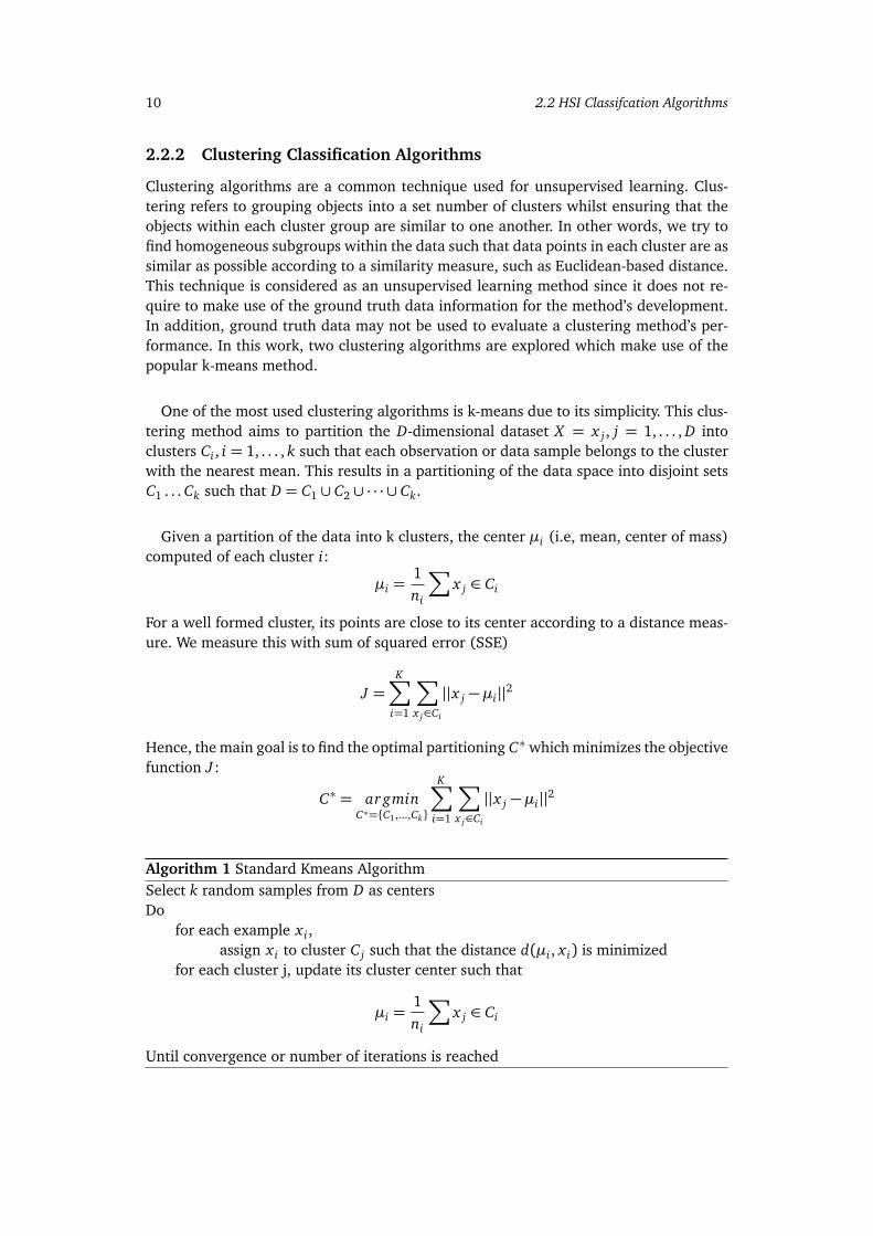
Clustering algorithms are a common technique used for unsupervised learning. Clus-tering refers to grouping objects into a set number of clusters whilst ensuring that theobjects within each cluster group are similar to one another. In other words, we try tofind homogeneous subgroups within the data such that data points in each cluster are assimilar as possible according to a similarity measure, such as Euclidean-based distance.This technique is considered as an unsupervised learning method since it does not re-quire to make use of the ground truth data information for the method’s development.In addition, ground truth data may not be used to evaluate a clustering method’s per-formance. In this work, two clustering algorithms are explored which make use of thepopular k-means method.
One of the most used clustering algorithms is k-means due to its simplicity. This clus-tering method aims to partition the D-dimensional dataset X = x j , j = 1, . . . , D intoclusters Ci , i = 1, . . . , k such that each observation or data sample belongs to the clusterwith the nearest mean. This results in a partitioning of the data space into disjoint setsC1 . . . Ck such that D = C1 ∪ C2 ∪ · · · ∪ Ck.
Given a partition of the data into k clusters, the center µi (i.e, mean, center of mass)computed of each cluster i:
µi =1ni
∑
x j ∈ Ci
For a well formed cluster, its points are close to its center according to a distance meas-ure. We measure this with sum of squared error (SSE)
J =K∑
i=1
∑
x j∈Ci
||x j −µi||2
Hence, the main goal is to find the optimal partitioning C∗ which minimizes the objectivefunction J :
C∗ = ar gminC∗={C1,...,Ck}
K∑
i=1
∑
x j∈Ci
||x j −µi||2
Algorithm 1 Standard Kmeans AlgorithmSelect k random samples from D as centersDo
for each example x i ,assign x i to cluster C j such that the distance d(µi , x i) is minimized
for each cluster j, update its cluster center such that
µi =1ni
∑
x j ∈ Ci
Until convergence or number of iterations is reached
Chapter 2: Background 11
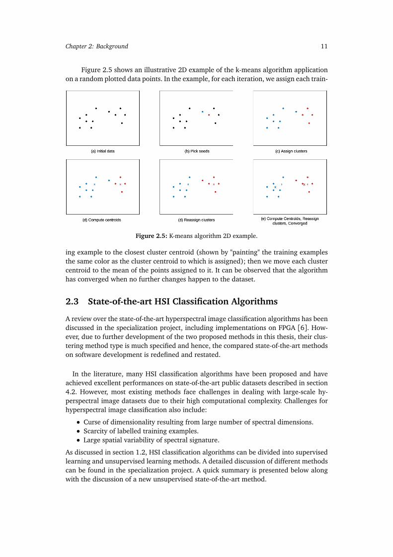
Figure 2.5 shows an illustrative 2D example of the k-means algorithm applicationon a random plotted data points. In the example, for each iteration, we assign each train-
Figure 2.5: K-means algorithm 2D example.
ing example to the closest cluster centroid (shown by "painting" the training examplesthe same color as the cluster centroid to which is assigned); then we move each clustercentroid to the mean of the points assigned to it. It can be observed that the algorithmhas converged when no further changes happen to the dataset.
2.3 State-of-the-art HSI Classification Algorithms
A review over the state-of-the-art hyperspectral image classification algorithms has beendiscussed in the specialization project, including implementations on FPGA [6]. How-ever, due to further development of the two proposed methods in this thesis, their clus-tering method type is much specified and hence, the compared state-of-the-art methodson software development is redefined and restated.
In the literature, many HSI classification algorithms have been proposed and haveachieved excellent performances on state-of-the-art public datasets described in section4.2. However, most existing methods face challenges in dealing with large-scale hy-perspectral image datasets due to their high computational complexity. Challenges forhyperspectral image classification also include:
• Curse of dimensionality resulting from large number of spectral dimensions.• Scarcity of labelled training examples.• Large spatial variability of spectral signature.
As discussed in section 1.2, HSI classification algorithms can be divided into supervisedlearning and unsupervised learning methods. A detailed discussion of different methodscan be found in the specialization project. A quick summary is presented below alongwith the discussion of a new unsupervised state-of-the-art method.
12 2.3 State-of-the-art HSI Classification Algorithms
2.3.1 Supervised vs. Unsupervised Learning Methods
The first step in a supervised learning method consists of transforming the image to afeature image to reduce the data dimensionality and improve the data interpretability.This processing phase comprises techniques such as principal component analysis (PCA).In the training phase, a set of training samples of the original image is selected andpatched to characterize each class. The classifier is trained using the training sampleswith certain parameters that affect the rate of learning. During the training process,a patch of test samples (ground truth data) is used to validate the classifier learningprogress and to find out if the classifier requires more training. Eventually, the classifierends up with an assignment criteria for each class label of a certain hyperspectral image.
High accurate supervised methods incorporate Convolution Neural Networks (CNNs),discussed in 2.2.1. These networks act like convolution filters to extract features whenapplied to data. They can be designed in 1D, 2D or 3D forms. The difference is thestructure of the input data and how the filter, also known as a convolution kernel orfeature detector, moves across the data.In the HSI context, it is evident from the literature that using just either 2D-CNN or 3D-CNN had a few shortcomings such as missing channel relationship information or verycomplex model, respectively [11]. The main reason is due to the fact that hyperspectralimages are volumetric data and have a spectral dimension as well. The 2D-CNN aloneisn’t able to extract good discriminating feature maps from the spectral dimensions.Similarly, a deep 3D-CNN is more computationally complex and alone seems to performworse for classes having similar textures over many spectral bands.In Feb 2019, a hybrid-CNN model which overcomes these shortcomings of the previousmodels have been proposed in [11]. It consists of 3D-CNN and 2D-CNN layers whichare assembled in such a way that they utilise both the spectral as well as spatial featuremaps to their full extent to achieve maximum possible accuracy.
HSI classification based on such supervised methods provide excellent performanceon standard datasets, e.g., more than 95% of the overall accuracy [11]. However, theseexisting methods face challenges in dealing with large-scale hyperspectral image data-sets due to their high computational complexity [5]. Challenges for hyperspectral imageclassification also include the "curse of dimensionality", resulting from large number ofspectral dimensions, and scarcity of labelled training examples as discussed earlier [12].
On the contrary, clustering-based techniques do not require prior knowledge andare commonly used for hyperspectral image unsupervised classification but still facechallenges due to high spectral resolution and presence of complex spatial struc-tures. Apart from removal of noisy or redundant bands, the optimal selection of spectralband(s) is one of the major tasks during classification for HSI. To address the high spec-tral resolution problem, the most common clustering approach utilizes feature extractionmethods for pre-processing such that one common subspace is produced for the wholedata set where clustering takes place. In [13], k-means clustering method was used toform different clusters from the data obtained after applying principal component ana-lysis (PCA) as a pre-processing technique. A local band selection approach is proposedin [14] where relevant set of bands is obtained using both relevancy and redundancy
Chapter 2: Background 13
among the spectral bands. This approach takes care of redundancy among the bands bymaking use of interband distances.
2.3.2 Segment-based Clustering
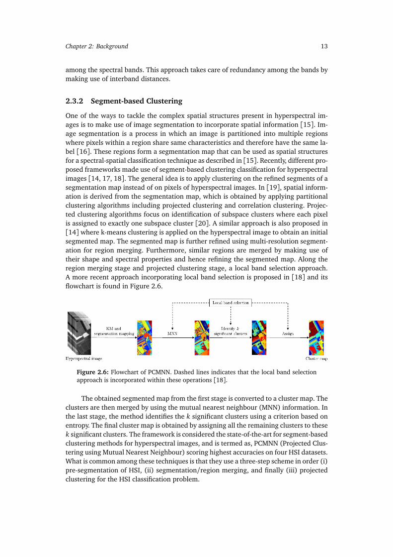
One of the ways to tackle the complex spatial structures present in hyperspectral im-ages is to make use of image segmentation to incorporate spatial information [15]. Im-age segmentation is a process in which an image is partitioned into multiple regionswhere pixels within a region share same characteristics and therefore have the same la-bel [16]. These regions form a segmentation map that can be used as spatial structuresfor a spectral-spatial classification technique as described in [15]. Recently, different pro-posed frameworks made use of segment-based clustering classification for hyperspectralimages [14, 17, 18]. The general idea is to apply clustering on the refined segments of asegmentation map instead of on pixels of hyperspectral images. In [19], spatial inform-ation is derived from the segmentation map, which is obtained by applying partitionalclustering algorithms including projected clustering and correlation clustering. Projec-ted clustering algorithms focus on identification of subspace clusters where each pixelis assigned to exactly one subspace cluster [20]. A similar approach is also proposed in[14] where k-means clustering is applied on the hyperspectral image to obtain an initialsegmented map. The segmented map is further refined using multi-resolution segment-ation for region merging. Furthermore, similar regions are merged by making use oftheir shape and spectral properties and hence refining the segmented map. Along theregion merging stage and projected clustering stage, a local band selection approach.A more recent approach incorporating local band selection is proposed in [18] and itsflowchart is found in Figure 2.6.
Figure 2.6: Flowchart of PCMNN. Dashed lines indicates that the local band selectionapproach is incorporated within these operations [18].
The obtained segmented map from the first stage is converted to a cluster map. Theclusters are then merged by using the mutual nearest neighbour (MNN) information. Inthe last stage, the method identifies the k significant clusters using a criterion based onentropy. The final cluster map is obtained by assigning all the remaining clusters to thesek significant clusters. The framework is considered the state-of-the-art for segment-basedclustering methods for hyperspectral images, and is termed as, PCMNN (Projected Clus-tering using Mutual Nearest Neighbour) scoring highest accuracies on four HSI datasets.What is common among these techniques is that they use a three-step scheme in order (i)pre-segmentation of HSI, (ii) segmentation/region merging, and finally (iii) projectedclustering for the HSI classification problem.
14 2.4 Binary Partition Trees and HSI
2.3.3 Method Choice
For HSI classification algorithms, in the context of the HYPSO mission objectives, theleading state-of-the-art supervised algorithm is the HybridSN CNN [11] with the fol-lowing classification accuracies: 99.99% on Pavia University dataset, 99.81% on In-dian Pines, and 100% on Salinas Scene. HybridSN seems to be the best choice for theHSI classification problem as it is the leading state-of-the-art algorithm, however, usingclustering-based method implementation on FPGAs is preferred for a number of reasons:
1. It is generally difficult to generalize the architecture of a very complex deep learn-ing model. Different layers have different parameters. The main challenge is thatCNN architectures do not usually have identical layer parameters, which increasesthe difficulty of designing generic hardware modules for the FPGA. For example,there are 1-D convolutional layers with different kernel sizes such as 3x1 and 5x1.
2. We notice that the recent developed CNNs are biased towards the 3 datasets (PaviaUniversity, Indian Pines, and Salinas Scene), which are land-cover based datasets,and hence might not perform well for other datasets such as Samson, Urban, andJasper Ridge which incorporate "water" as one of the classes. CNNs might also notperform well on such datasets because images may not be of the expected highquality or the dataset itself is small.
3. The highest classification reached for the HSI classification problem is approxim-ately 100% on the 3 datasets. Hence, there is a tendency in research for improvingthe other classification methods, e.g. clustering, so that it performs better for otherdatasets, including small datasets or unlabeled datasets which is not efficient forCNNs to learn from. In this study, 8 HSI datasets are experimented on, which areboth land-cover and water based images.
4. The simple control flow and inherent parallelism of distance computations makesclustering suitable for dedicated hardware implementations such as FPGAs andthis found to be proven in [21].
Based on the specialization project [6] and the method choice above, this thesispresents implementations of clustering-type unsupervised classification algorithms forhyperspectral images. Two algorithms are implemented in software; a novel segment-based clustering algorithm and a spectral clustering algorithm. Furthermore, based oncoming experiments and analysis in Chapter 4, the spectral clustering method is imple-mented for FPGA. Necessary background information for both hardware and softwareimplementations is detailed in the sections below.
2.4 Binary Partition Trees and HSI
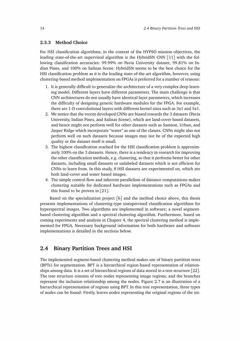
The implemented segment-based clustering method makes use of binary partition trees(BPTs) for segmentation. BPT is a hierarchical region-based representation of relation-ships among data. It is a set of hierarchical regions of data stored in a tree structure [22].The tree structure consists of tree nodes representing image regions, and the branchesrepresent the inclusion relationship among the nodes. Figure 2.7 is an illustration of ahierarchical representation of regions using BPT. In this tree representation, three typesof nodes can be found: Firstly, leaves nodes representing the original regions of the ini-

Chapter 2: Background 15
tial image partition; secondly, the root node representing the entire image support andfinally, the remaining tree nodes representing regions formed by the merging of theirtwo child nodes corresponding to two adjacent regions. Each of these non leaf nodeshas at most two child nodes, this is why the BPT is defined as binary.
Figure 2.7: Example of hierarchical region-based representation using BPT [9].
In the context of hyperspectral images, a BPT representation is generated using(i) a given region model and (ii) a region merging criterion, both recently developedby [9]. Given the initial partition of small regions, the BPT is constructed in such a waythat the most meaningful regions of the images are represented by nodes. The leaf nodescorrespond to the initial partition of the image. From this initial partition, an iterativebottom-up region merging algorithm is applied by keeping track of the merging stepswhere the most similar adjacent regions are merged at each iteration until only oneregion remains. This last region represents the whole image and is the root of the tree.The creation of BPT relies on three important notions:
1. The method obtaining the initial partition, also called, pre-segmentation.2. The region model MRi
which defines how regions are represented and how tomodel the union of two regions.
3. The merging criterion O(MRi, MR j
), which defines the similarity of neighboring re-gions as a distance measure between the region models MRi
and MR jand involves
determining the order in which regions are going to be merged.
In [9], different region models with their compatible region merging criterion were de-scribed to construct the BPT.
2.4.1 Pre-segmentation using Watershed Method
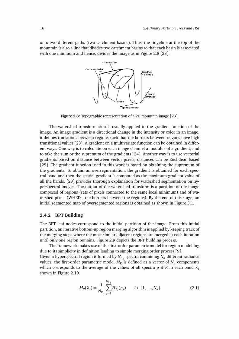
A watershed is a transformation defined on a grayscale image. To perform watershedsegmentation, a 2D image is viewed as a topographic map that shows hills and valleys asit can be observed in Figure 2.8. In that map/image, the value of each pixel correspondsto the elevation at that pixel point. Thus, dark areas (low pixel value) are valleys, whilebright areas (high pixel value) are hills. The watershed transform finds catchment basins(or dark areas) in this landscape. For example, when it rains on a mountain, water slides
16 2.4 Binary Partition Trees and HSI
onto two different paths (two catchment basins). Thus, the ridgeline at the top of themountain is also a line that divides two catchment basins so that each basin is associatedwith one minimum and hence, divides the image as in Figure 2.8 [23].
Figure 2.8: Topographic representation of a 2D mountain image [23].
The watershed transformation is usually applied to the gradient function of theimage. An image gradient is a directional change in the intensity or color in an image,it defines transitions between regions such that the borders between reigons have hightransitional values [23]. A gradient on a multivariate function can be obtained in differ-ent ways. One way is to calculate on each image channel a modulus of a gradient, andto take the sum or the supremum of the gradients [24]. Another way is to use vectorialgradients based on distance between vector pixels, distances can be Euclidean-based[25]. The gradient function used in this work is based on obtaining the supremum ofthe gradients. To obtain an oversegmentation, the gradient is obtained for each spec-tral band and then the spatial gradient is computed as the maximum gradient value ofall the bands. [23] provides thorough explanation for watershed segmentation on hy-perspectral images. The output of the watershed transform is a partition of the imagecomposed of regions (sets of pixels connected to the same local minimum) and of wa-tershed pixels (WHEDs, the borders between the regions). By the end of this stage, aninitial segmented map of oversegmented regions is obtained as shown in Figure 3.1.
2.4.2 BPT Building
The BPT leaf nodes correspond to the initial partition of the image. From this initialpartition, an iterative bottom-up region merging algorithm is applied by keeping track ofthe merging steps where the most similar adjacent regions are merged at each iterationuntil only one region remains. Figure 2.9 depicts the BPT building process.
The framework makes use of the first-order parametric model for region modellingdue to its simplicity in definition leading to simple merging order process [9].Given a hyperspectral region R formed by NRp
spectra containing Nn different radiancevalues, the first-order parametric model MR is defined as a vector of Nn componentswhich corresponds to the average of the values of all spectra p ∈ R in each band λishown in Figure 2.10.
MR(λi) =1
NRp
NRp∑
j=1
Hλi(p j) i ∈ [1, . . . , Nn] (2.1)

Chapter 2: Background 17
Figure 2.9: BPT construction using a region merging algorithm [9].
Note that Hλi(p j) represents the radiance value in the wavelength λi of the pixel
whose spatial coordinates are p j .
Figure 2.10: A grid representing the set of spectra for a region R containing M pixelsand modelled into one column of spectra.
Using the first-order parametric model (2.1), a merging criterion is defined as thespectral angle distance, dSAD, between the average values of any two adjacent regions:
O(MRa, MRb
) = dSAD = arccos
�
RTa Rb
||Ra||||Rb||
�
, (2.2)
18 2.4 Binary Partition Trees and HSI
where Ra, Rb are two different regions and MRa, MRb
are their corresponding spectrumcolumn region model.The region merging stage runs until there are no more mutual best neighbours availablefor merging. Further, before merging regions, small and meaningless regions in the initialpartition of the previous stage may result in a spatially unbalanced tree during BPTconstruction. Those regions are prioritized to be merged first in the region mergingorder by determining whether they are smaller than a given percentage (typically 15%)regions created by the merging process of the average region size of the initial partition[9].
2.4.3 BPT Pruning
Until this point, we have obtained a BPT representation of the hyperspectral image incor-porating its spatial and spectral features. The next step is to process the BPT such that weget a partition featuring the N most dissimilar regions created during the constructionof the binary partition tree. This can be done by extracting a given number of regionsPR (pruned regions), hence pruning the tree. Different BPT pruning strategies lead todifferent results [26]. Furthermore, there exists several BPT pruning strategies suitedfor a number of applications like classification, segmentation, and object detection [27,28].
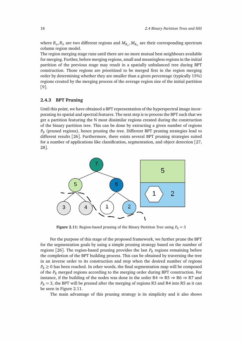
Figure 2.11: Region-based pruning of the Binary Partition Tree using PR = 3
For the purpose of this stage of the proposed framework, we further prune the BPTfor the segmentation goals by using a simple pruning strategy based on the number ofregions [26]. The region-based pruning provides the last PR regions remaining beforethe completion of the BPT building process. This can be obtained by traversing the treein an inverse order to its construction and stop when the desired number of regionsPR ≥ 0 has been reached. In other words, the final segmentation map will be composedof the PR merged regions according to the merging order during BPT construction. Forinstance, if the building of the nodes was done in the order R4⇒ R5⇒ R6⇒ R7 andPR = 3, the BPT will be pruned after the merging of regions R3 and R4 into R5 as it canbe seen in Figure 2.11.
The main advantage of this pruning strategy is its simplicity and it also shows

Chapter 2: Background 19
whether the BPT was constructed in a meaningful way or not since the last PR regionsare the most dissimilar regions. By the end of this stage, a well refined segmentationmap of the hyperspectral image is obtained which can be further used by a k-meansfiltering algorithm.
2.5 Filtering Algorithm
K-means algorithm complexity goes up linearly in k centres, the number of data pointsand the number of dimensions in a dataset, and the number of iterations [29]. This isbecause a straightforward implementation of k-means standard algorithm can be quiteslow due to the cost of computing nearest neighbors; we want to find the minimumargument for each cluster group and calculate the distances of each point in a cluster tothe centroid of that cluster. Thus, it becomes infeasible in high dimensional spaces withmany data points such as hyperspectral images.
Furthermore, getting the argmin of the objective function J defined in section 2.2.2 iscomputationally expensive for hyperspectral images [29]. In [30], a filtering algorithmwas developed for a multidimensional binary search tree, called a k-d tree. A k-d tree isa space partitioning tree data structure for organizing data points in a K-Dimensionalspace. The main goal of the filtering algorithm is to prune (filter) down the search spacefor the optimal partition such that the computation burden is reduced [21]. In this work,we make use of the filtering algorithm for another binary tree structure that allowsflexibility in region splitting (BPT discussed in section 2.4).
Figure 2.12: Candidate z is pruned because C lies entirely on one side of the bisectinghyperplane H [8].
Assume that the hyperspectral image is segmented into regions using a segment-ation method and is represented by a binary tree structure such that the leaves of thetree represent the partitions within the HSI cube. At the initial iteration of clustering,the regions of the segmentation map act as a base for the algorithm to start from. Dur-ing clustering, these regions are either differentiated or joined by assigning them clusterlabels as the tree is traversed for a number of iterations.Algorithm 2 shows pseudo code for one iteration of the filtering algorithm. Each tree

20 2.5 Filtering Algorithm
node u represents a region and is associated with the bounding box (C) information aswell as the number of pixels (count) and the vector sum of the associated pixels (theweighted centroid, wgtCent) which is used to update the cluster centres when eachiteration of the algorithm completes. The actual centroid is just wgtCent/count. In ad-dition, for each node of the tree, we maintain a set of possible candidate centers Z thatis propagated down the tree. This is defined to be a set of center points that can be thenearest neighbor for some pixel within a tree node. It follows that the candidate centersfor the root node consist of all k centers.
For a tree node u, the closest candidate center z∗ ∈ Z to the midpoint of the bound-ing box is found during clustering. The closest centre search involves the computationof the Euclidean distances. The remaining z ∈ Z \ {z∗} is pruned to the following nodedown the tree if no part of C is closer to z than the closest centre z∗ since it is not thenearest center to the pixels within C . Figure 2.12 shows an illustration where the set ofpoints are enclosed by the closed cell C and z∗ is the closest center point to the points inC . Hence, the center z is not further considered as a center since no part of C is closerto z than to z∗ and z is removed from the center candidate list for the closed cell C . Ifu is an internal node, we recurse on its children. The centre update occurs if a leaf isreached or only one candidate remains.
Algorithm 2 The filtering algorithm introduced in [30]function Filter (kdNode u, CandidateSet Z) {C ← u.Cif (u is a leaf) {
z∗← the closest point in Z to u.pointz∗.wgtCent ← z∗.wgtCent + u.pointz ∗ .count ← z∗.count + 1 }
else {z∗← the closest point in Z to C’s midpointfor all (z ∈ Z \ {z∗}) do
if z.isFarther(z∗, C) then Z ← Z \ {z}end forif (|Z |= 1) {
z∗.wgtCent ← z∗.wgtCent + u.wgtCentz ∗ .count ← z∗.count + u.count }
else {Filter(u.le f t, Z)Filter(u.ri ght, Z) }
}}for all (z ∈ Z)
z← z.wgtCent/z.count
The isFar ther function of Algorithm 2 checks whether any point of a boundingbox C is closer to z than to z∗. The function returns true if the sum of squares differ-ence between the candidate z and the closest candidate z∗ is greater than 2 × the sum ofsquares difference between either boundary points (high or low) and the closest candid-
Chapter 2: Background 21
ate center z∗. On termination of the filtering algorithm, center z is moved to the centroidof its associated points, that is, z← z.wgtCent/z.count.
2.6 Spectral Clustering
Spectral clustering techniques are widely used, due to their simplicity and empirical per-formance advantages compared to other clustering methods, such as k-means [31]. Thistype of clustering can be solved efficiently by standard linear algebra methods. The basicidea is to represent each data point as a graph-node and thus transform the clusteringproblem into a graph-partitioning problem. Thus, the goal is to identify communities ofnodes in a graph based on the edges connecting them. A typical implementation con-sists of two fundamental steps: 1. Building a similarity graph and 2. Finding an optimalpartition of the constructed graph.
2.6.1 Building the Similarity Graph
Given a set of data point samples x1, . . . , xn, the method first builds a similarity graphG = {Ver t ices, Ed ges} such that each vertex represents a sample x i and the edge toanother point x j is weighted by the similarity wi j where wi j is positive or larger than acertain threshold. The problem of clustering can now be reformulated using the similar-ity graph: we want to find a partition of the graph such that the edges between differentgroups have very low weights where points in different clusters are dissimilar from eachother, and the edges within a group have high weights such that points within the samecluster are similar to each other.In general, the corresponding similarity (or affinity) matrix W can be denoted as
Wi j = exp−||x i − x j||22
2σ2, i, j = 1, 2, . . . , n, (2.3)
whereσ is the width of the neighbors of the samples and n is the number of graph nodes.
2.6.2 Finding an Optimal Partition
Let A and B represent a bipartition of Vertices, where A ∪ B = Vertices and A ∩ B =;. The simplest and most direct way to construct a partition of the graph is to solvethe minimum cut (mincut) problem. For a given number k of subsets, the mincut ap-proach simply consists in choosing a partition A1, . . . , Ak which minimizes cut(A,B) =∑
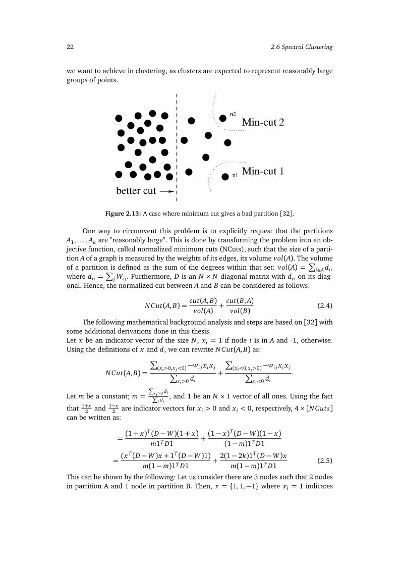
i∈A, j∈B Wi j . Hence, cut(A,B) denotes the sum of the weights between A and B. In thiscase, there are two partitions, k = 2, and the mincut problem is relatively easy to solve[31]. However, in practice the solution often does not lead to satisfactory partitions. Theproblem is that in many cases, the solution of mincut simply separates one individualvertex from the rest of the graph. Figure 2.13 illustrates such case. Assuming the edgeweights are inversely proportional to the distance between the two nodes, it can be ob-served that the cut partitioning node n1 or n2 will have a very small value. In fact, anycut that partitions out individual nodes on the right half will have smaller cut value thanthe cut that partitions the nodes into the left and right halves. Of course this is not what
22 2.6 Spectral Clustering
we want to achieve in clustering, as clusters are expected to represent reasonably largegroups of points.
Figure 2.13: A case where minimum cut gives a bad partition [32].
One way to circumvent this problem is to explicitly request that the partitionsA1, . . . , Ak are "reasonably large". This is done by transforming the problem into an ob-jective function, called normalized minimum cuts (NCuts), such that the size of a parti-tion A of a graph is measured by the weights of its edges, its volume vol(A). The volumeof a partition is defined as the sum of the degrees within that set: vol(A) =
∑
i∈A diiwhere dii =
∑
j Wi j . Furthermore, D is an N × N diagonal matrix with dii on its diag-onal. Hence, the normalized cut between A and B can be considered as follows:
NCut(A, B) =cut(A, B)
vol(A)+
cut(B, A)vol(B)
(2.4)
The following mathematical background analysis and steps are based on [32] withsome additional derivations done in this thesis.Let x be an indicator vector of the size N , x i = 1 if node i is in A and -1, otherwise.Using the definitions of x and d, we can rewrite NCut(A, B) as:
NCut(A, B) =
∑
(x i>0,x j<0)−wi j x i x j∑
x i>0 di+
∑
(x i<0,x j>0)−wi j x i x j∑
x i<0 di.
Let m be a constant; m =∑
xi>0 di∑
i di, and 1 be an N × 1 vector of all ones. Using the fact
that 1+x2 and 1−x
2 are indicator vectors for x i > 0 and x i < 0, respectively, 4× [NCuts]can be written as:
=(1+ x)T (D−W )(1+ x)
m1T D1+(1− x)T (D−W )(1− x)
(1−m)1T D1
=(x T (D−W )x + 1T (D−W )1)
m(1−m)1T D1+
2(1− 2k)1T (D−W )xm(1−m)1T D1
(2.5)
This can be shown by the following: Let us consider there are 3 nodes such that 2 nodesin partition A and 1 node in partition B. Then, x = {1,1,−1} where x i = 1 indicates

Chapter 2: Background 23
that the node belongs to A, otherwise, it belongs to B. Then the first numerator part ofNCut(A,B) is:
∑
(x i>0,x j<0)
−wi j x i x j = −w13 x1 x3 −w23 x2 x3 = w13 +w23.
Hence, 4× [NCuts] (1st part numerator) can be written as:
(1+ x)T (D−W )(1+ x) =>�
2 2 0�
w12 +w13 −w12 −w13−w21 w21 +w23 −w23−w31 −w32 w31 +w32
220
This is equal to 4 × (w13 + w23) as expected. A similar argument can be made for the2nd part of the numerator of 4× [NCuts].As for the denominator part,
m=
∑
x i>0 di∑
i di=
w11 +w12 +w21 +w22 +w13 +w23
w11 +w12 +w13 +w21 +w22 +w13 +w23 +w33,
then,
m1T D1=w11 +w12 +w21 +w22 +w13 +w23
w11 +w12 +w13 +w21 +w22 +w13 +w23 +w33×
(w11 +w12 +w13 +w21 +w22 +w13 +w23 +w33) =∑
x i>0
di .
Letα(x) = x T (D−W )x ,
β(x) = 1T (D−W )x ,
γ= 1T (D−W )1,
andQ = 1T D1,
then, Equation 2.5 can be further expanded as:
=(α(x) + γ) + 2(1− 2m)β(x)
m(1−m)Q
=(α(x) + γ) + 2(1− 2m)β(x)
m(1−m)Q−
2(α(x) + γ)Q
+2α(x)
Q+
2γQ
.
Dropping the last constant term such that it equals to 0, we get
=(1− 2m+ 2m2)(α(x) + γ) + 2(1− 2m)β(x)
m(1−m)Q+
2(α(x) + γ)Q
=1−2m+2m2
(1−m)2 (α(x) + γ) +2(1−2m)(1−m)2 β(x)
m(1−m)Q
+2α(x)
Q.
24 2.6 Spectral Clustering
Since γ= 0, then 2bγbQ = 0 and letting b = m
(1−m) , it becomes
=(1+ b2)(α(x) + γ) + 2(1− b2)β(x)
bQ+
2bα(x)bQ
=(1+ b2)(α(x) + γ) + 2(1− b2)β(x)
bQ+
2bα(x)bQ
−2bγbQ
.
Substituting back, it becomes
=(1+ b2)(x T (D−W )x + 1T (D−W )1)
b1T D1+
2(1− b2)1T (D−W )xb1T D1
+2b(x T (D−W )x)
b1T D1−
2b1T (D−W )1b1T D1
=(1+ x)T (D−W )(1+ x)
b1T D1+
b2(1− x)T (D−W )(1− x)b1T D1
−2b(1− x)T (D−W )(1+ x)
b1T D1
=(1+ x)T (D−W )(1+ x)
b1T D1+
b2(1− x)T (D−W )(1− x)b1T D1
−2b(1− x)T (D−W )(1+ x)
b1T D1.
Using matrix transpose properties, we get
=[(1+ x)− b(1− x)T (D−W )[(1+ x)− b(1− x)]
b1T D1. (2.6)
The goal now is to formulate expression 2.6 such that we find a minimum objectivefunction with conditions.Setting y = (1+ x)− b(1− x), where (1+ x) is a vector with all the nodes in the partitionA (x i > 0) and the vector (1− x) is otherwise (x i < 0). And since (A− B)T = AT − BT ,we can see that
y T D1=∑
x i>0
di − b∑
x i<0
di =∑
x i>0
di − (m
1−m)∑
x i<0
di
=∑
x i>0
di −
∑
x i>0 di∑
x i<0 di
∑
x i<0
di = 0.
We can deduce that
y T D y =∑
x i>0
di + b2∑
x i<0
di = b∑
x i<0
di + b2∑
x i<0
di
= b(∑
x i<0
di + b∑
x i<0
di)
= b1T D1
Hence, the minimum objective function for expression 2.6 becomes
minx Ncut(x) = minyy T (D−W )y
y T D y(2.7)
with the condition y T D1= 0.The right hand side of Equation 2.7 is the Rayleigh quotient if y is relaxed to take on

Chapter 2: Background 25
real values such that the matrices and vectors are real [32]. Hence, the problem can beminimized by solving the generalized eigenvalue system:
(D−W )y = λD y. (2.8)
Let z = D12 y , then the generalized eigenvalue system 2.8 becomes
(D−W )D−12 z = λDD−
12 z,
multiply D−12 on both sides,
D−12 (D−W )D−
12 z = λD−
12 DD−
12 z,
D−12 (D−W )D−
12 z = λz. (2.9)
We reach the standard eigensystem 2.9 which is to be minimized.Note that D −W is considered the "Laplacian Matrix" L. The Laplacian is just anothermatrix representation of a graph which has the following properties:
• L is a positive semidefinite matrix.• The smallest eigenvalue of an eigensystem of L is 0, the corresponding eigenvector
is the constant 1 vector.• L has n non-negative, real-valued eigenvalues such that 0= λ1 ≤ λ2 ≤ . . .λn.
According to spectral graph theory, an approximate resolution of Equation 2.7 can beconsidered as thresholding the eigenvector corresponding to the second smallest eigen-values of the normalized Laplacian L. The second smallest nonzero eigenvalue is calledthe spectral gap. The spectral gap gives us some notion of the density of the graph. If thisgraph was densely connected (all pairs of the n nodes had an edge), then the spectralgap would be n, where n is number of nodes.
The direct relation between the eigenvalues of a Laplacian matrix and clustering issummarized below:
• When the nodes in a graph are completely disconnected, then all eigenvalues are0.
• Otherwise, the 1st eigenvalue is always 0 since there is only one connected com-ponent which is the graph itself.
• The 2nd eigenvalue approximates the minimum graph cut needed to separate thegraph into two connected components.
• Near zero 2nd eigenvalue shows that there is almost a separation of two compon-ents.
• Each value in the 2nd eigenvector gives us information about which side of thecut a node belongs to, either positive or negative.
Algorithm 3 summarizes shows the established spectral clustering algorithm.
26 2.6 Spectral Clustering
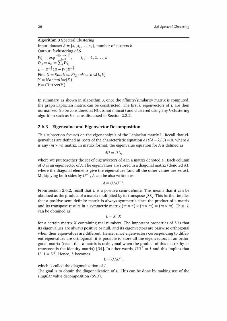
Algorithm 3 Spectral ClusteringInput: dataset S = {s1, s2, . . . , sn}, number of clusters kOutput: k-clustering of S
Wi j = exp−||x i−x j ||22
2σ2 , i, j = 1,2, . . . , nDi j = dii =
∑
j Wi j
L = D−12 (D−W )D−
12
Find X = SmallestEigenVectors(L, k)Y = Normalize(X )k = Cluster(Y )
In summary, as shown in Algorithm 3, once the affinity/similarity matrix is computed,the graph Laplacian matrix can be constructed. The first k eigenvectors of L are thennormalized (to be considered as NCuts not mincut) and clustered using any k-clusteringalgorithm such as k-means discussed in Section 2.2.2.
2.6.3 Eigenvalue and Eigenvector Decomposition
This subsection focuses on the eigenanalysis of the Laplacian matrix L. Recall that ei-genvalues are defined as roots of the characteristic equation det(A−λIm) = 0, where Ais any (m×m) matrix. In matrix format, the eigenvalue equation for A is defined as
AU = UΛ,
where we put together the set of eigenvectors of A in a matrix denoted U . Each columnof U is an eigenvector of A. The eigenvalues are stored in a diagonal matrix (denoted Λ),where the diagonal elements give the eigenvalues (and all the other values are zeros).Multiplying both sides by U−1, A can be also written as
A= UΛU−1.
From section 2.6.2, recall that L is a positive semi-definite. This means that it can beobtained as the product of a matrix multiplied by its transpose [33]. This further impliesthat a positive semi-definite matrix is always symmetric since the product of a matrixand its transpose results in a symmetric matrix (m× n)× (n×m) = (m×m). Thus, Lcan be obtained as:
L = X T X
for a certain matrix X containing real numbers. The important properties of L is thatits eigenvalues are always positive or null, and its eigenvectors are pairwise orthogonalwhen their eigenvalues are different. Hence, since eigenvectors corresponding to differ-ent eigenvalues are orthogonal, it is possible to store all the eigenvectors in an ortho-gonal matrix (recall that a matrix is orthogonal when the product of this matrix by itstranspose is the identity matrix) [34]. In other words, UU T = I and this implies thatU−1= U T . Hence, L becomes
L = UΛU T ,
which is called the diagonalization of L.The goal is to obtain the diagonalization of L. This can be done by making use of thesingular value decomposition (SVD).
Chapter 2: Background 27
Singular Value Decomposition
According to [35], for a rectangular matrix A (m×n), let p = min{m, n} the SVD theoremstates that
A= UΣV T , where
• U = (u1, . . . , um) ∈ Rm×m is orthogonal.• V = (v1, . . . , vn) ∈ Rn×n is orthogonal.• Σ= diag(σ1, . . . ,σp) ∈ Rm×n,σ1 ≥ σ2 ≥ · · · ≥ σp ≥ 0.
σi are called the singular values, ui are the left singular vectors, and vi are the rightsingular vectors. The singular values, σi , are the square roots of the eigenvalues of AT Aand of AAT (these two matrices have the same eigenvalues).
Corollary 1 If A is a symmetric matrix the singular values are the absolute values of theeigenvalues of A : σi = |λi| and the columns of U = V are the eigenvectors of A.
PROOF: If A is symmetric then AAT = AT A= A2 and U , V,Σ are square matrices. The ei-genvectors of A are also the eigenvectors of A2 with squared corresponding eigenvalues.The singular values are the absolute values of the eigenvalues of A. �
This implies that for the symmetric matrix L, L = UΛU T is the SVD of L where U andΛ are the eigenvalues and the eigenvectors of L, respectively. Hence, finding the SVD ofthe Laplacian matrix corresponds to finding its eigenvalue decomposition.
Jacobi Method
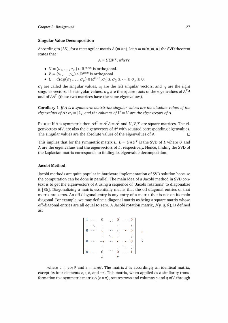
Jacobi methods are quite popular in hardware implementation of SVD solution becausethe computation can be done in parallel. The main idea of a Jacobi method in SVD con-text is to get the eigenvectors of A using a sequence of "Jacobi rotations" to diagonalizeit [36]. Diagonalizing a matrix essentially means that the off-diagonal entries of thatmatrix are zeros. An off-diagonal entry is any entry of a matrix that is not on its maindiagonal. For example, we may define a diagonal matrix as being a square matrix whoseoff-diagonal entries are all equal to zero. A Jacobi rotation matrix, J(p, q,θ ), is definedas:
where c = cosθ and s = sinθ . The matrix J is accordingly an identical matrix,except its four elements c, s, c, and −s. This matrix, when applied as a similarity trans-formation to a symmetric matrix A (n×n), rotates rows and columns p and q of A through

28 2.6 Spectral Clustering
the angle θ so that the (p, q) and (q, p) off-diagonal entries are zeroed as shown below(∗ is any entry ai j):
∗ · · · ∗. . .
app · · · apq...
.... . .
......
aqp · · · aqq. . .
∗ · · · ∗
→
∗ · · · ∗. . .
a′pp · · · 0...
.... . .
......
0 · · · a′qq. . .
∗ · · · ∗
.
Based on the number of angles required for annihilating the off-diagonal elements, Jac-obi methods are broadly classified as One-sided and Two-sided Jacobi methods. Two-sided Jacobi method is implemented in this work. The simplified stages of Two-sidedJacobi for solving eigenfunction problems can be described as:
1. Choose an index pair (p,q) from matrix A such that 1< p < q < n.2. Calculate a (c,s) pair for the rotation matrix J such that the 2 × 2 subproblem
matrix is diagonal:
�
a′pp a′pqa′qp a′qq
�
=
�
c1 s1−s1 c1
�T �app apqaqp aqq
��
c2 s2−s2 c2
�
(2.10)
3. Repeat by selecting the next (p,q) pairs. The algorithm fetches the next index pair(p, q) such for a sequence of N jacobi rotations, called sweep. The matrix A isoverwritten at each step A← J T A J .
The 2nd stage involves solving for off-diagonal elements and equating to zero (a′pq anda′qp are equal to zero):
app.sinθ1cosθ2 + aqp.cosθ1cosθ2 − apq.sinθ1sinθ2 + aqq.cosθ1sinθ2 = 0, (2.11)
app.cosθ1sinθ2 − aqp.sinθ1sinθ2 − apq.cosθ1cosθ2 + aqq.sinθ1cosθ2 = 0. (2.12)
Adding and subtracting Equations 2.11 and 2.12, gives the required Jacobi rotationangles:
tan(θ1 + θ2) =apq + aqp
aqq − app; tan(θ1 − θ2) =
apq − aqp
aqq + app. (2.13)
θ1 and θ2 are called half angles. The goal is to diagonalize matrix A in terms of θ1 andθ2. Equation 2.10 can be re-written as:
�
a′pp 00 a′qq
�
=
�
cosθ1 −sinθ1sinθ1 cosθ1
��
app.cosθ2 − apq.sinθ2 app.sinθ2 + apq.cosθ2aqp.cosθ2 − aqq.sinθ2 aqp.sinθ2 + aqq.cosθ2
�
(2.14)Replace cosθ1 ⇒ c1, sinθ1 ⇒ s1, cosθ2 ⇒ c2, and sinθ2 ⇒ s2, and carry out matrixmultiplication of Equation 2.14, a′pp and a′qq become:
a′pp = c1.(app.c2− apq.s2)− s1.(aqp.c2− aqq.s2), (2.15)
Chapter 2: Background 29
a′qq = s1.(app.s2+ apq.c2) + c1.(aqp.s2+ aqq.c2). (2.16)
Hence, the rotation angles cos(θ1+θ2), cos(θ1−θ2), sin(θ1+θ2), sin(θ1−θ2) canall be obtained by solving Equation 2.13. Thus, a solution is obtained for a′pp and a′qq in�
a′pp 00 a′qq
�
. The Two-sided Jacobi algorithm for SVD is formulated in Algorithm 4.
Algorithm 4 Two-sided Jacobi for eigenvalues and eigenvectors.Step 1. Read the symmetric matrix A. Let U = 1 be a matrix of the same size as A.
Step 2. Construct matrix U and V that are identical to the unit matrix, except for
Upp = Uqq = Vpp = Vqq = cosθ , Upq = Vpq = sinθ , and Uqp = Vqp = −sinθ .
Step 3. Find the off-diagonal element from A= [apq].
Step 4. Find the rotational angles using Equation 2.13. And hence, find U ′ and V ′
Step 5. Then compute the matrix products A′ = V T AU , Uout = U ′.U , and Vout = V ′.V ;
A′pq becomes zero by this operation, the other elements in rows and columns p and q
are changed.
Step 6. If the number of iterations is reached or the largest absolute value of the off
diagonal elements Apq is larger than a threshold, repeat the process from step no. 3
with A′ instead of A, Uout instead of U , and Vout instead of V . Upon convergence, A′
contains the eigenvalues, and Uout and Vout contain the eigenvectors.
Algorithm 4 concludes with singular value decomposition of the symmetric matrix A.
2.6.4 Spectral Clustering Example
For illustration, consider a graph G with 5 vertices, the similarity matrix for the graphis found using some criterion to be for example:
W =
0 1 1 0 01 0 1 0 01 1 0 1 00 0 1 0 10 0 0 1 0
An entry in the matrix W , wi j represents whether node i and j share an edge. The graphcorresponding to matrix W is presented below: It can be observed that for example thatnode 1 shares 3 edges with nodes 2,3, and 5, hence, the entries (1,2),(1,3),(1,5) areones in the matrix W . In addition, the diagonal entries of W are zero.The degree matrix D discussed earlier represents the sum of weights for each node, i.e.,

30 2.6 Spectral Clustering
Figure 2.14: Similarity graph corresponding to matrix W .
number of connections each node has. In this example the degree matrix D becomes:
D =
2 0 0 0 00 2 0 0 00 0 3 0 00 0 0 2 00 0 0 0 1
The degree of node i j = 11 is 2 in this case.The Laplacian matrix L can be found by L = D−W :
L =
2 −1 −1 0 0−1 2 −1 0 0−1 −1 3 −1 00 0 −1 2 −10 0 0 −1 1
The diagonal of L represents the degrees of the nodes while off the diagonal are binaryentries of 0 or -1; 0 means that a pair of given nodes is not connected and -1 that thepair of nodes is connected. Next step is to find the eigenvalues of the matrix L.First, we compute LLT and LT L. Using Corollary 1, we know that LLT = LT L = L2,then L2 is:
L =
6 −3 −4 1 0−3 6 −4 1 0−4 −4 12 −5 11 1 −5 6 −30 0 1 −3 2
We can determine the eigenvalues of the matrix L2 using the roots of the characteristicequation det(L2 −λIm) = 0.
det
6 −3 −4 1 0−3 6 −4 1 0−4 −4 12 −5 11 1 −5 6 −30 0 1 −3 2
−λ
1 0 0 0 00 1 0 0 00 0 1 0 00 0 0 1 00 0 0 0 1
: −λ5+32λ4−306λ3+916λ2−225λ
= −λ(λ4 − 32λ3 + 306λ2 − 916λ+ 225) = −λ(λ− 9)(λ3 − 23λ2 + 99λ− 25) = 0.
Chapter 2: Background 31
Solving the last equation gives the sorted eigenvalues of L2:
λ1 = 0λ2 = 0.269λ3 = 5.341λ4 = 9
λ5 = 17.390
Hence, the singular values (eigenvalues of L) are σi =p
λi sorted:
σ1 = 0σ2 = 0.5188σ3 = 2.311λ4 = 3λ5 = 4.17
We find that the first eigenvalue of L, σ1, is 0 as expected. The eigenvalues aresorted to find the 2nd smallest eigenvalue, λ2 = 0.5188 where the corresponding vectoris:
−0.59696−0.59696−0.287250.48119
1
The nodes on the graph can be labelled with 0 or 1 classes according to each value inthe eigenvector (positive or negative). It gives us information about which side of thecut a node belongs to.
Extensions to multiple partitions are possible via recursive bipartitioning or throughthe use of multiple eigenvectors. In this work, we make use of multiple eigenvectors tofind partitions of more than just 2 clusters. This is done by spectral embedding. Spec-tral embedding aims to represent a graph in some Euclidean space of low dimension,say RNE where NE � n. Hence, each node i ∈ V is represented by vector ei ∈ RE . Thestructure of the graph must be encoded in its representation e1, e2, . . . , en such that twoclose nodes i, j in the graph G correspond to two close vectors ei , e j in the embeddingspace.The importance of spectral embedding in spectral clustering can be shown in Figure2.15. Mapping the nodes of the graph into higher dimensions shows the distances betweenthe nodes. Eigenvectors of the Laplacian matrix provide an embedding of the data basedon similarity, i.e, groups the closer nodes together. To find such an embedding for thenormalized cut problem, [37] computed the n× NE matrix of the leading eigenvectorsV and the NE × NE diagonal matrix of eigenvalues Λ of the system:
D−12 (D−W )D−
12 V = VΛ.
The ith embedding representation of the jth pixel is then given by
Ei j =Vi+1, jÆ
Dj j, i = 1, . . . , NE , j = 1, . . . , N , (2.17)
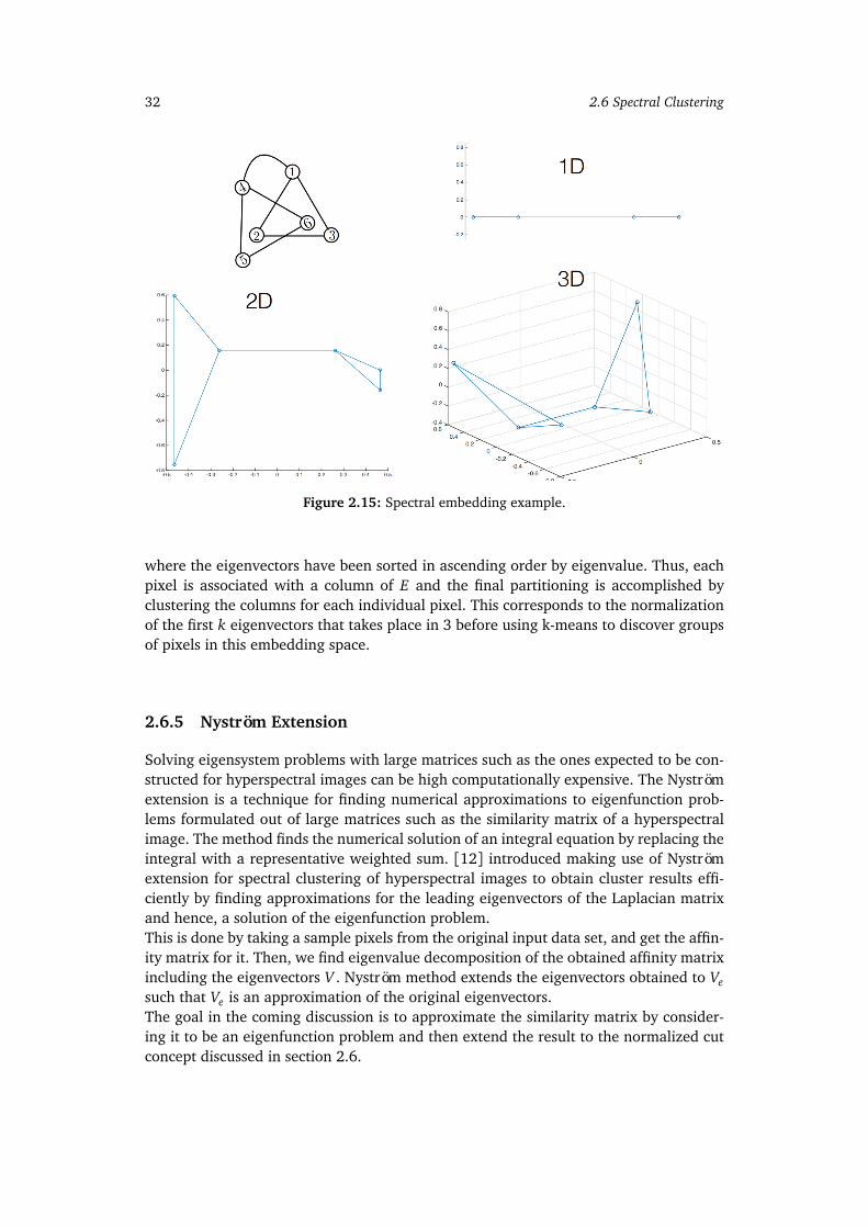
32 2.6 Spectral Clustering
Figure 2.15: Spectral embedding example.
where the eigenvectors have been sorted in ascending order by eigenvalue. Thus, eachpixel is associated with a column of E and the final partitioning is accomplished byclustering the columns for each individual pixel. This corresponds to the normalizationof the first k eigenvectors that takes place in 3 before using k-means to discover groupsof pixels in this embedding space.
2.6.5 Nyström Extension
Solving eigensystem problems with large matrices such as the ones expected to be con-structed for hyperspectral images can be high computationally expensive. The Nyströmextension is a technique for finding numerical approximations to eigenfunction prob-lems formulated out of large matrices such as the similarity matrix of a hyperspectralimage. The method finds the numerical solution of an integral equation by replacing theintegral with a representative weighted sum. [12] introduced making use of Nyströmextension for spectral clustering of hyperspectral images to obtain cluster results effi-ciently by finding approximations for the leading eigenvectors of the Laplacian matrixand hence, a solution of the eigenfunction problem.This is done by taking a sample pixels from the original input data set, and get the affin-ity matrix for it. Then, we find eigenvalue decomposition of the obtained affinity matrixincluding the eigenvectors V . Nyström method extends the eigenvectors obtained to Vesuch that Ve is an approximation of the original eigenvectors.The goal in the coming discussion is to approximate the similarity matrix by consider-ing it to be an eigenfunction problem and then extend the result to the normalized cutconcept discussed in section 2.6.
Chapter 2: Background 33
In the context of hyperspectral images, the affinity matrix considers both the reflect-ance value of the pixels and their spatial location in order to define the similarity betweentwo samples x i and x j . Hence, equation 2.3 of section 2.6 can be redefined as:
Wi j = exp−||li − l j||22
2σ2l
. exp−||x i − x j||22
2σ2x
, i, j = 1, 2, . . . , n, (2.18)
where li and l j are the spatial locations of the HSI’s pixels and σl and σx are thebandwidth of neighbouring pixels. σl and σx are sensitive to different hyperspectralimages. According to [38], these parameters can be related to li and l j and x i and x j ,and we can define σl and σx as
σl =1n2
n∑
i=1
n∑
j=1
||li − l j||22, σx =1n2
n∑
i=1
n∑
j=1
||x i − x j||22. (2.19)
Substituting back to Equation 2.8, it becomes:
Wi j = exp−||li − l j||22
2ασl2 . exp
−||x i − x j||222ασx
2 , i, j = 1, 2, . . . , n, (2.20)
where α is a parameter or factor to control the number of neighbors for each node inthe affinity matrix.
Let A be a matrix defined by Equation 2.18, then A is an affinity matrix of m chosensamples. The similarity matrix of the remaining n−m samples and the chosen samplesare denoted as B. In addition, let C denote the affinity matrix for the remaining samplesalone. The affinity matrix W of equation 2.8 can be rewritten as
W =
�
A BBT C
�
, (2.21)
where BT is the transpose of matrix B. Hence, A∈ Rm×m, B ∈ Rm×n, and C ∈ Rn×n.The affinity matrix C can be extremely large for HSI images. According to Nyströmextension, if we know A and B we can find an approximation for matrix C such thatC = BT A−1B. In other words, given only m rows of the matrix W , we can find the valuesof the entire n× n matrix W . In the following discussion, we establish the explanationof Nyström extension method in the steps similiar to [39].
Eigenfunction problems in which the Nyström extension is used are in the form
∫ b
aW (x , y)φ(y)dy = λφ(x).
According to [39], we can approximate this integral equation by evaluating it at a setof evenly spaced points ε1,ε2, . . . ,εn on the interval [a, b] and employing an approx-imation (called, quadrature rule; more information can be found in Appendix 2) of thedefinite integral of the function W (x , y)φ(y) such that it becomes:

34 2.6 Spectral Clustering
(b− a)n
n∑
j=1
W (x ,ε j)φ(ε j) = λφ(x), (2.22)
where φ(x) is an approximation to the true φ(x). Set x = εi and equation 2.22becomes
(b− a)n
n∑
j=1
W (εi ,ε j)φ(ε j) = λφ(εi) ∀i ∈ {1 . . . n}. (2.23)
Let [a, b] be [0,1], we structure the system 2.23 as a matrix eigenvalue problem:
AbΦ= nbΦΛ
where Ai j =W (εi ,ε j) and bΦ= [φ1, φ2, . . . , φn] are the n eigenvectors of A corres-ponding to λ1,λ2, . . . ,λn placed on the diagonals of the matrix Λ. Substituting back toequation 2.22 yields the Nyström extension for each eigenvector φi:
φi(x) =1
nλi
n∑
j=1
W (x ,ε j)φi(ε j). (2.24)
This expression allows us to extend an eigenvector computed for a set of sample pointsto an arbitrary point x using W (.,ε j) as the interpolation weights.
Considering A again to be the affinity matrix present in matrix W of Equation 2.21. Ithas been established in Section 2.6 that the Laplacian matrix is a positive semi-definitematrix. Recall the eigenvalue decomposition analysis of A from Section 2.6.3:
A= UΛU T
which is called the diagonalization of A.Going back to the Nyström extension for φi in 2.24, since matrix B represents the weightsbetween the sample points and the remaining points, then, the matrix form of the Nys-tröm extension is BT UΛ−1 where BT corresponds to W (ε j , .), the columns of U , theeigenvector, corresponds to φi(ε j)s, and Λ−1 corresponds to 1/λis. Recall the matrix Wof 2.21, letting U denote the approximate eigenvectors of W , then
U =
�
UBT UΛ−1
�
, (2.25)
since U is the eigenvectors of A and BT UΛ−1 is the Nyström extension matrix form.Furthermore, we can approximate W , which we denote, cW , such that
Chapter 2: Background 35
cW = UΛU T (2.26)
=
�
UBT UΛ−1
�
Λ�
U T Λ−1U T B�
(2.27)
=
�
UΛU T BBT BT A−1B
�
(2.28)
=
�
A BBT BT A−1B
�
(2.29)
=
�
AB
�
A−1�
A B�
(2.30)
(2.31)
since UU T = I = ΛΛ−1. Hence, C = BT A−1B according to the approximation of thematrix W using Nyström extension.
We are left to extend the above approximation to the normalized cut defined earlierin section 2.6. We know that by definition, bd represent the row sum of matrix W , hence,
bd =cW1=
�
A1m + B1nBT 1m + BT A−1B1n
�
, (2.32)
where A1m and B1n are the row sum of matrices A and B and BT 1m is the columnsum of matrix B. 1m is a vector row of 1s of size m.Having d, we can approximate the blocks of D−
12 (D−W )D−
12 , (similar to the embedding
done in Equation 2.17) such that the matrix A and B can be formulated as:
Ai j =Ai j
Ç
ÒdiÒd j
(2.33)
Bi j =Bi j
Ç
Òdibd j+m
(2.34)
and we can get the normalized affinity matrix D−12cW D−
12 , hence,
D−12cW D−
12 =
�
AB
�
A−1�
A B�
. (2.35)
In summary, Algorithm 3 becomes

36 2.7 Overview of Zynq-7000 Functional Blocks
Algorithm 5 Spectral Clustering with Nyström extension method [37].Input: dataset S = {s1, s2, . . . , sn}, number of clusters kOutput: k-clustering of S
Wi j = exp−||li−l j ||22
2σ2l
. exp−||x i−x j ||22
2σ2x
, i, j = 1, 2, . . . , n.
Di j = dii =∑
j Wi j .Calculate matrices A and B using Equations 2.33 and 2.34.Compute the normalized Laplacian
L = D−12cW D−
12 =
�
AB
�
A−1�
A B�
.
Find v1, v2, . . . , vk = SmallestEigenVectors(L, k).Let V ∈ Rn×k be the matrix containing the vectors v1, v2, . . . , vk as columns.Find the embedding Ei j =
Vi+1, jpD j j
, i, j = 1, . . . , k.
For i = 1, . . . , n, let yi ∈ Rk be the vector corresponding to the i-th row of E.Cluster the points (yi)i=1,,...,n in Rk with the k-means algorithm into clusters C1, . . . , Ck.
2.7 Overview of Zynq-7000 Functional Blocks
Zynq-7000 is a family of Xilinx System-on-Chip (SoC) products which offers the flexib-ility and scalability of an FPGA, while providing performance, power, and ease of use.The SoC architecture enables implementation of custom logic in the processing logic(PL) and custom software in the processing system (PS), and thus, enables implement-ations of HW/SW co-designs. The overview of the Zynq architecture is shown in Figure2.16, showing the functional blocks of both the PL and the PS.The processing system comprises four major blocks:
• Application Processor Unit (APU) which includes 2 ARM Cortex-A9 cores.• Memory Interfaces: A dynamic memory controller and static memory interface
modules.• I/O Peripherals (IOP) which contains the data communication peripherals.• Central Interconnect through which the APU, memory interface unit, and the IOP
are all connected to each other and to the PL.
Making use of the four main blocks of the PS along with a special PS-PL interface allowshigh performance communication between PS and PL cores on a single chip, whichfurther makes HW/SW co-design implementations possible. The processing logic coresused in this thesis include DSP blocks, BRAM blocks, and DMA core. The PS-PL interfaceis conducted by AXI protocols explained below in this section.
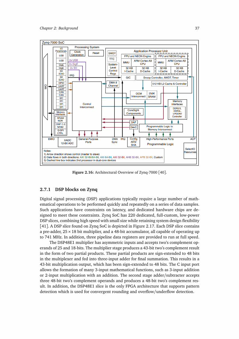
Chapter 2: Background 37
Figure 2.16: Architectural Overview of Zynq-7000 [40].
2.7.1 DSP blocks on Zynq
Digital signal processing (DSP) applications typically require a large number of math-ematical operations to be performed quickly and repeatedly on a series of data samples.Such applications have constraints on latency, and dedicated hardware chips are de-signed to meet these constraints. Zynq SoC has 220 dedicated, full-custom, low-powerDSP slices, combining high speed with small size while retaining system design flexibility[41]. A DSP slice found on Zynq SoC is depicted in Figure 2.17. Each DSP slice containsa pre-adder, 25×18 bit multiplier, and a 48-bit accumulator, all capable of operating upto 741 MHz. In addition, three pipeline data registers are provided to run at full speed.
The DSP48E1 multiplier has asymmetric inputs and accepts two’s complement op-erands of 25 and 18-bits. The multiplier stage produces a 43-bit two’s complement resultin the form of two partial products. These partial products are sign-extended to 48 bitsin the multiplexer and fed into three-input adder for final summation. This results in a43-bit multiplication output, which has been sign-extended to 48 bits. The C input portallows the formation of many 3-input mathematical functions, such as 3-input additionor 2-input multiplication with an addition. The second stage adder/subtracter acceptsthree 48-bit two’s complement operands and produces a 48-bit two’s complement res-ult. In addition, the DSP48E1 slice is the only FPGA architecture that supports patterndetection which is used for convergent rounding and overflow/underflow detection.
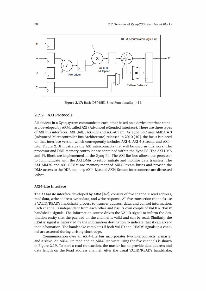
38 2.7 Overview of Zynq-7000 Functional Blocks
Figure 2.17: Basic DSP48E1 Slice Functionality [41].
2.7.2 AXI Protocols
All devices in a Zynq system communicate each other based on a device interface stand-ard developed by ARM, called AXI (Advanced eXtended Interface). There are three typesof AXI bus interfaces: AXI (full), AXI-lite and AXI-stream. As Zynq SoC uses AMBA 4.0(Advanced Microcontroller Bus Architecture) released in 2010 [40], the focus is placedon that interface version which consequently includes AXI-4, AXI-4 Stream, and AXI4-Lite. Figure 2.18 illustrates the AXI interconnects that will be used in this work. Theprocessor and DDR memory controller are contained within the Zynq PS. The AXI DMAand PL Block are implemented in the Zynq PL. The AXI-lite bus allows the processorto communicate with the AXI DMA to setup, initiate and monitor data transfers. TheAXI_MM2S and AXI_S2MM are memory-mapped AXI4-Stream buses and provide theDMA access to the DDR memory. AXI4-Lite and AXI4-Stream interconnects are discussedbelow.
AXI4-Lite Interface
The AXI4-Lite interface developed by ARM [42], consists of five channels: read address,read data, write address, write data, and write response. All five transaction channels usea VALID/READY handshake process to transfer address, data, and control information.Each channel is independent from each other and has its own couple of VALID/READYhandshake signals. The information source drives the VALID signal to inform the des-tination entity that the payload on the channel is valid and can be read. Similarly, theREADY signal is generated by the information destination to indicate that it can acceptthat information. The handshake completes if both VALID and READY signals in a chan-nel are asserted during a rising clock edge.
Communication over an AXI4-Lite bus incorporates two interconnects, a masterand a slave. An AXI4-Lite read and an AXI4-Lite write using the five channels is shownin Figure 2.19. To start a read transaction, the master has to provide data address anddata length on the Read address channel. After the usual VALID/READY handshake,
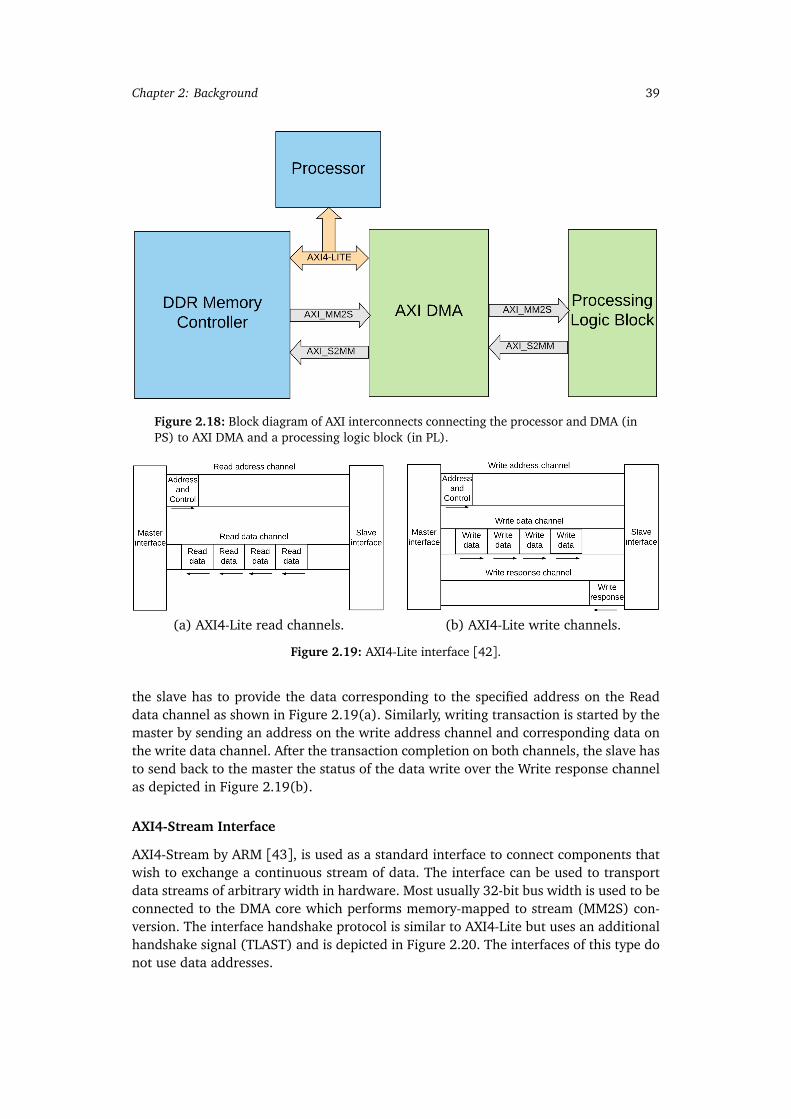
Chapter 2: Background 39
Figure 2.18: Block diagram of AXI interconnects connecting the processor and DMA (inPS) to AXI DMA and a processing logic block (in PL).
(a) AXI4-Lite read channels. (b) AXI4-Lite write channels.
Figure 2.19: AXI4-Lite interface [42].
the slave has to provide the data corresponding to the specified address on the Readdata channel as shown in Figure 2.19(a). Similarly, writing transaction is started by themaster by sending an address on the write address channel and corresponding data onthe write data channel. After the transaction completion on both channels, the slave hasto send back to the master the status of the data write over the Write response channelas depicted in Figure 2.19(b).
AXI4-Stream Interface
AXI4-Stream by ARM [43], is used as a standard interface to connect components thatwish to exchange a continuous stream of data. The interface can be used to transportdata streams of arbitrary width in hardware. Most usually 32-bit bus width is used to beconnected to the DMA core which performs memory-mapped to stream (MM2S) con-version. The interface handshake protocol is similar to AXI4-Lite but uses an additionalhandshake signal (TLAST) and is depicted in Figure 2.20. The interfaces of this type donot use data addresses.

40 2.7 Overview of Zynq-7000 Functional Blocks
Figure 2.20: AXI4-Stream Interface.
In AXI4-Stream, TDATA width of bits is transferred per clock cycle. The transferis started once the master signals TVALID and the slave responds with TREADY whichrepresents that it is ready to receive data. TLAST signals the last byte of the stream.TUSER is an optional signal which is a user defined sideband information that can betransmitted alongside the data stream [43]. In addition, TID and TDEST are two op-tional signals where TID usually identifies which master the stream originated from,and TDEST is used to route the stream to the appropriate destination.
2.7.3 AXI DMA
Direct Memory Access (DMA) cores are used to allow direct memory access to peripher-als with minimal CPU intervention. In the case of a Zynq system, AXI DMA provided byXilinx [44], is instantiated in PL and it is used to transfer data from DDR memory to theFPGA cores with AXI-stream interfaces as shown in Figure 2.18. The AXIS_MM2S andAXIS_S2MM are AXI4-streaming buses, which source and sink a continuous stream ofdata without addresses. In this work, we use the DMA to transfer data from memory toan PL block and back to the memory. In principle, the PL block could be any kind of dataproducer/consumer. In our case, it is the processing logic block of the intended HW/SWco-design.
2.7.4 Block RAM
One of the main challenges in hardware implementation of matrix operations is storingthe data. As the real symmetric matrix is quite huge, it needs to be stored in memoryand filled into and pulled from the memory to perform operations on it. The Xilinx blockRAM (BRAM) is a dual-port RAM module instantiated into the FPGA fabric to provideon-chip storage for a relatively large set of data. Zynq-7000 features 36Kb BRAM dual-port units which allow for parallel, same-clock-cycle access to different locations [45].In this work, the BRAM is modified such that it has 1 write and 2 read ports for a vectorof data. In other words, there are two read pointers to data addresses which can bedecoded into 2 separate or the same data row. Figure 2.21 shows the design of a dual-port vector BRAM with write enable (we) used in this work. The BRAM is defined by itssize (BRAM_ADDR_WIDTH) and width of each row (BRAM_DATA_WIDTH). For a writeoperation, din represents the input data to be written on the RAM address specified bythe row (w_addr) on the BRAM. Each row is associated with a write enable signal (we).

Chapter 2: Background 41
On the other hand, on each rising clock edge, the specified addresses, r_addr_1 andr_addr_2, are read and given to dout_1 and dout_2, respectively.
Figure 2.21: Vector storage using BRAM.
Figure 2.22: Vivado HLS Design Flow [46].
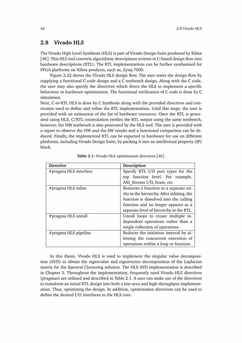
42 2.8 Vivado HLS
2.8 Vivado HLS
The Vivado High-Level Synthesis (HLS) is part of Vivado Design Suite produced by Xilinx[46]. This HLS tool converts algorithmic descriptions written in C-based design flow intohardware descriptions (RTL). The RTL implementations can be further synthesized forFPGA platforms on Xilinx products, such as, Zynq-7000.
Figure 2.22 shows the Vivado HLS design flow. The user starts the design flow bysupplying a functional C code design and a C testbench design. Along with the C code,the user may also specify the directives which direct the HLS to implement a specificbehaviour or hardware optimization. The functional verification of C code is done by Csimulation.Next, C-to-RTL HLS is done by C Synthesis along with the provided directives and con-straints used to define and refine the RTL implementation. Until this stage, the user isprovided with an estimation of the list of hardware resources. Once the RTL is gener-ated using HLS, C/RTL cosimulation verifies the RTL output using the same testbench,however, the HW testbench is also generated by the HLS tool. The user is provided witha report to observe the HW and the SW results and a functional comparison can be de-duced. Finally, the implemented RTL can be exported to hardware for use on differentplatforms, including Vivado Design Suite, by packing it into an intellectual property (IP)block.
Table 2.1: Vivado HLS optimization directives [46].
Directive Description#pragma HLS interface Specify RTL I/O port types for the
top function level. For example,AXI_Stream I/O, bram, etc.
#pragma HLS inline Removes a function as a separate en-tity in the hierarchy. After inlining, thefunction is dissolved into the callingfunction and no longer appears as aseparate level of hierarchy in the RTL.
#pragma HLS unroll Unroll loops to create multiple in-dependent operations rather than asingle collection of operations.
#pragma HLS pipeline Reduces the initiation interval by al-lowing the concurrent execution ofoperations within a loop or function.
In this thesis, Vivado HLS is used to implement the singular value decomposi-tion (SVD) to obtain the eigenvalue and eigenvector decomposition of the Laplacianmatrix for the Spectral Clustering solution. The HLS SVD implementation is describedin Chapter 5. Throughout the implementation, frequently used Vivado HLS directives(pragmas) are utilized and described in Table 2.1. A user can make use of the directivesto transform an initial RTL design into both a low-area and high-throughput implement-ation. Thus, optimizing the design. In addition, optimization directives can be used todefine the desired I/O interfaces to the HLS core.
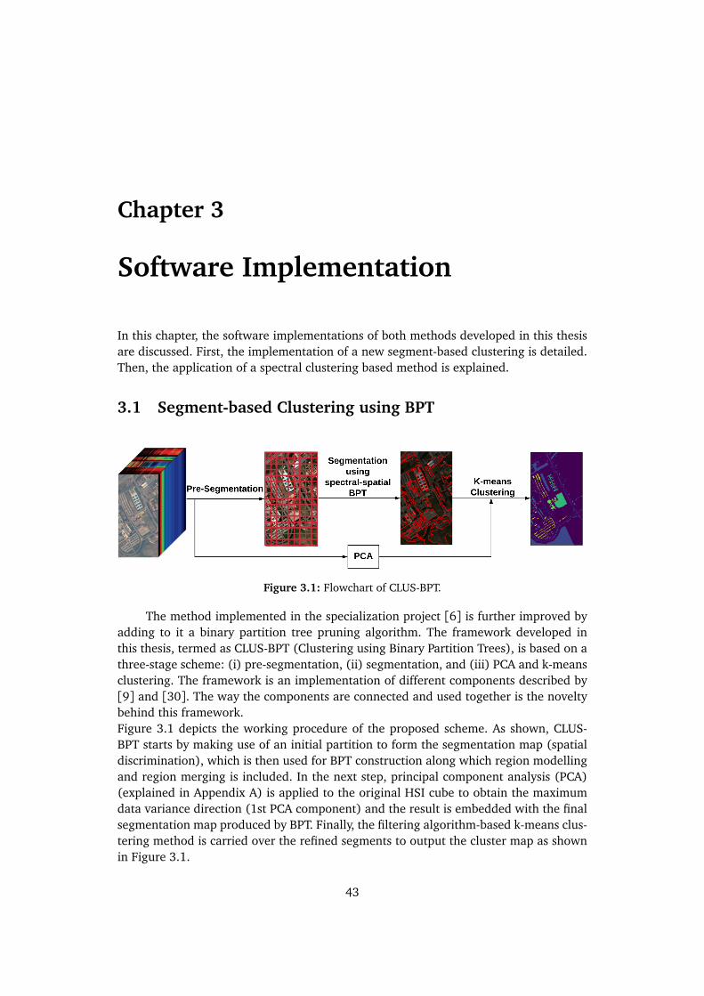
Chapter 3
Software Implementation
In this chapter, the software implementations of both methods developed in this thesisare discussed. First, the implementation of a new segment-based clustering is detailed.Then, the application of a spectral clustering based method is explained.
3.1 Segment-based Clustering using BPT
Figure 3.1: Flowchart of CLUS-BPT.
The method implemented in the specialization project [6] is further improved byadding to it a binary partition tree pruning algorithm. The framework developed inthis thesis, termed as CLUS-BPT (Clustering using Binary Partition Trees), is based on athree-stage scheme: (i) pre-segmentation, (ii) segmentation, and (iii) PCA and k-meansclustering. The framework is an implementation of different components described by[9] and [30]. The way the components are connected and used together is the noveltybehind this framework.Figure 3.1 depicts the working procedure of the proposed scheme. As shown, CLUS-BPT starts by making use of an initial partition to form the segmentation map (spatialdiscrimination), which is then used for BPT construction along which region modellingand region merging is included. In the next step, principal component analysis (PCA)(explained in Appendix A) is applied to the original HSI cube to obtain the maximumdata variance direction (1st PCA component) and the result is embedded with the finalsegmentation map produced by BPT. Finally, the filtering algorithm-based k-means clus-tering method is carried over the refined segments to output the cluster map as shownin Figure 3.1.
43
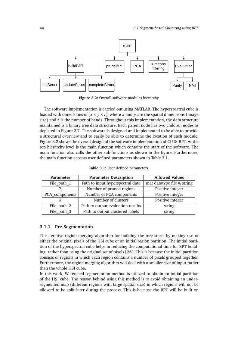
44 3.1 Segment-based Clustering using BPT
Figure 3.2: Overall software modules hierarchy.
The software implementation is carried out using MATLAB. The hyperspectral cube isloaded with dimensions of (x× y×z), where x and y are the spatial dimensions (imagesize) and z is the number of bands. Throughout this implementation, the data structuremaintained is a binary tree data structure. Each parent node has two children nodes asdepicted in Figure 2.7. The software is designed and implemented to be able to providea structural overview and to easily be able to determine the location of each module.Figure 3.2 shows the overall design of the software implementation of CLUS-BPT. At thetop hierarchy level is the main function which contains the start of the software. Themain function also calls the other sub-functions as shown in the figure. Furthermore,the main function accepts user defined parameters shown in Table 3.1.
Table 3.1: User defined parameters.
Parameter Parameter Description Allowed ValuesFile_path_1 Path to input hyperspectral data mat datatype file & string
PR Number of pruned regions Positive integerPCA_components Number of PCA components Positive integer
k Number of clusters Positive integerFile_path_2 Path to output evaluation results stringFile_path_3 Path to output clustered labels string
3.1.1 Pre-Segmentation
The iterative region merging algorithm for building the tree starts by making use ofeither the original pixels of the HSI cube or an initial region partition. The initial parti-tion of the hyperspectral cube helps in reducing the computational time for BPT build-ing, rather than using the original set of pixels [26]. This is because the initial partitionconsists of regions in which each region contains a number of pixels grouped together.Furthermore, the region merging algorithm will deal with a smaller size of input ratherthan the whole HSI cube.In this work, Watershed segmentation method is utilized to obtain an initial partitionof the HSI cube. The reason behind using this method is to avoid obtaining an under-segmented map (different regions with large spatial size) in which regions will not beallowed to be split later during the process. This is because the BPT will be built on
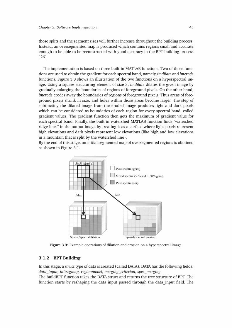
Chapter 3: Software Implementation 45
those splits and the segment sizes will further increase throughout the building process.Instead, an oversegmented map is produced which contains regions small and accurateenough to be able to be reconstructed with good accuracy in the BPT building process[26].
The implementation is based on three built-in MATLAB functions. Two of those func-tions are used to obtain the gradient for each spectral band, namely, imdilate and imerodefunctions. Figure 3.3 shows an illustration of the two functions on a hyperspectral im-age. Using a square structuring element of size 3, imdilate dilates the given image bygradually enlarging the boundaries of regions of foreground pixels. On the other hand,imerode erodes away the boundaries of regions of foreground pixels. Thus areas of fore-ground pixels shrink in size, and holes within those areas become larger. The step ofsubtracting the dilated image from the eroded image produces light and dark pixelswhich can be considered as boundaries of each region for every spectral band, calledgradient values. The gradient function then gets the maximum of gradient value foreach spectral band. Finally, the built-in watershed MATLAB function finds "watershedridge lines" in the output image by treating it as a surface where light pixels representhigh elevations and dark pixels represent low elevations (like high and low elevationsin a mountain that is split by the watershed line).By the end of this stage, an initial segmented map of oversegmented regions is obtainedas shown in Figure 3.1.
Figure 3.3: Example operations of dilation and erosion on a hyperspectral image.
3.1.2 BPT Building
In this stage, a struct type of data is created (called DATA). DATA has the following fields:data_input, initsegmap, regionmodel, merging_criterion, spec_merging.The buildBPT function takes the DATA struct and returns the tree structure of BPT. Thefunction starts by reshaping the data input passed through the data_input field. The
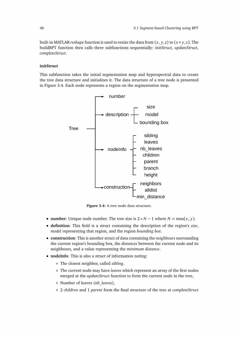
46 3.1 Segment-based Clustering using BPT
built-in MATLAB reshape function is used to resize the data from (x , y, z) to (x×y, z). ThebuildBPT function then calls three subfunctions sequentially: initStruct, updateStruct,completeStruct.
initStruct
This subfunction takes the initial segmentation map and hyperspectral data to createthe tree data structure and initializes it. The data structure of a tree node is presentedin Figure 3.4. Each node represents a region on the segmentation map.
Figure 3.4: A tree node data structure.
• number: Unique node number. The tree size is 2 ∗ N − 1 where N =max(x , y).
• definition: This field is a struct containing the description of the region’s size,model representing that region, and the region bounding box.
• construction: This is another struct of data containing the neighbours surroundingthe current region’s bounding box, the distances between the current node and itsneighbours, and a value representing the minimum distance.
• nodeInfo: This is also a struct of information noting:
◦ The closest neighbor, called sibling.
◦ The current node may have leaves which represent an array of the first nodesmerged at the updateStruct function to form the current node in the tree,
◦ Number of leaves (nb_leaves),
◦ 2 children and 1 parent form the final structure of the tree at completeStruct
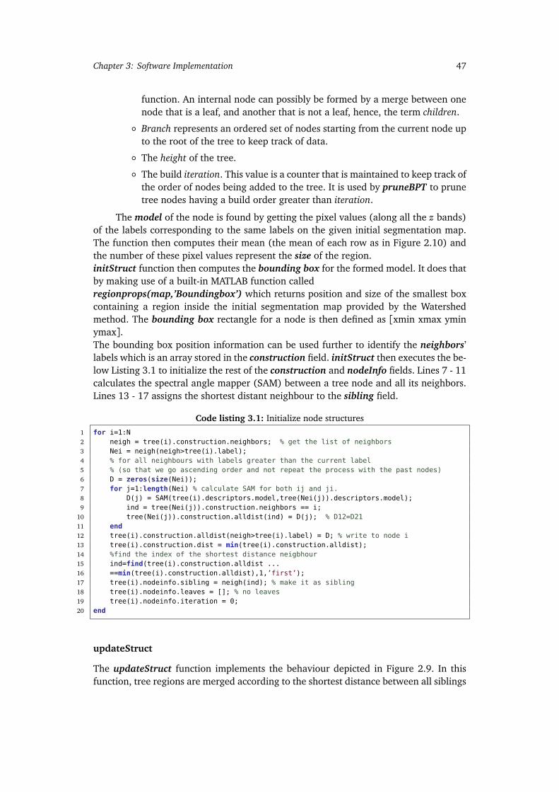
Chapter 3: Software Implementation 47
function. An internal node can possibly be formed by a merge between onenode that is a leaf, and another that is not a leaf, hence, the term children.
◦ Branch represents an ordered set of nodes starting from the current node upto the root of the tree to keep track of data.
◦ The height of the tree.
◦ The build iteration. This value is a counter that is maintained to keep track ofthe order of nodes being added to the tree. It is used by pruneBPT to prunetree nodes having a build order greater than iteration.
The model of the node is found by getting the pixel values (along all the z bands)of the labels corresponding to the same labels on the given initial segmentation map.The function then computes their mean (the mean of each row as in Figure 2.10) andthe number of these pixel values represent the size of the region.initStruct function then computes the bounding box for the formed model. It does thatby making use of a built-in MATLAB function calledregionprops(map,’Boundingbox’) which returns position and size of the smallest boxcontaining a region inside the initial segmentation map provided by the Watershedmethod. The bounding box rectangle for a node is then defined as [xmin xmax yminymax].The bounding box position information can be used further to identify the neighbors’labels which is an array stored in the construction field. initStruct then executes the be-low Listing 3.1 to initialize the rest of the construction and nodeInfo fields. Lines 7 - 11calculates the spectral angle mapper (SAM) between a tree node and all its neighbors.Lines 13 - 17 assigns the shortest distant neighbour to the sibling field.
Code listing 3.1: Initialize node structures
1 for i=1:N2 neigh = tree(i).construction.neighbors; % get the list of neighbors3 Nei = neigh(neigh>tree(i).label);4 % for all neighbours with labels greater than the current label5 % (so that we go ascending order and not repeat the process with the past nodes)6 D = zeros(size(Nei));7 for j=1:length(Nei) % calculate SAM for both ij and ji.8 D(j) = SAM(tree(i).descriptors.model,tree(Nei(j)).descriptors.model);9 ind = tree(Nei(j)).construction.neighbors == i;
10 tree(Nei(j)).construction.alldist(ind) = D(j); % D12=D2111 end12 tree(i).construction.alldist(neigh>tree(i).label) = D; % write to node i13 tree(i).construction.dist = min(tree(i).construction.alldist);14 %find the index of the shortest distance neigbhour15 ind=find(tree(i).construction.alldist ...16 ==min(tree(i).construction.alldist),1,’first’);17 tree(i).nodeinfo.sibling = neigh(ind); % make it as sibling18 tree(i).nodeinfo.leaves = []; % no leaves19 tree(i).nodeinfo.iteration = 0;20 end
updateStruct
The updateStruct function implements the behaviour depicted in Figure 2.9. In thisfunction, tree regions are merged according to the shortest distance between all siblings

48 3.1 Segment-based Clustering using BPT
for all tree nodes, this defines the merging order, which is an array of tree node labels tobe merged together in ascending order. However, as discussed in Chapter 2, small andmeaningless regions are prioritized to be merged first. Regions are considered smallif their size is less than a percentage (alpha) of the mean region size for the initialsegmentation map.In Listing 3.2, the MATLAB function starts by sorting all tree node sibling distances whilekeeping label information. Next, an inspection for small region sizes is done and themerging order is updated accordingly.
Code listing 3.2: Update node structures - Step 1.
1 D = [tree.construction];2 D = [D.dist]; % list of all distances3 [D,merging_order] = sort(D,’ascend’);4 % Step 1: find the merging order5 alpha = 0.15;6 Nregions = length(merging_order);7 mean_size_region = size(map,1)/Nregions; % mean size of a region8 thresh = round(alpha*mean_size_region); % threshold for small regions9 F = regsize(merging_order)<thresh;
10 % F is a flag binary vector where 1 means that the concerned regions gets11 % the merging priority12 merging_id = find(F,1,’first’); % find the ID of the first 1 in F13 if isempty(merging_id)14 % if no siblings have priority merging, merge the first two siblings15 merging_id = 1;16 end
The next step involves retrieving the two merging nodes information by making use ofmerging_id as in Listing 3.3. The following step creates a new node structure where themerging occurs. Lines 13-23 perform the sibling node merging for the descriptors field.The updatenewnode function in Line 24 updates the nodeInfo and construction fieldsof the tree. This is done by marking node i and node j as the children of the new label,transferring node i and node j neighbours to the new node, recalculating SAM distancesbetween the new node and those neighbours, and finally, marking node i and node jas leaves if both nodes do not have leaves from a previous update. The merging orderarray is then updated and the next two siblings are fetched and merged. The loop keepsgoing until two regions are remaining.
Code listing 3.3: Update node structures - Steps 2, 3, & 4.
1 %Step 2: retrieve the two regions which are to merge2 for i=1:N_iteration-2 % looping until there are two regions remaining3 % make a copy of the merging nodes4 node_i = tree(merging_order(merging_id));5 node_j = tree(S(merging_id)); % S is a list of siblings6 %empty the info about the first node merged7 S(merging_id) = []; merging_order(merging_id) = [];8 D(merging_id) = []; F(merging_id) = [];9 % Step 3: Create the new structure in tree
10 newlabel = N_iteration+i;11 tree(newlabel).label = newlabel;12 % merge the two models by multiplying the two models by their sizes13 Si = node_i.descriptors.size;14 Sj = node_j.descriptors.size;15 tree(newlabel).descriptors.size = Si+Sj;16 %field model17 Ri = node_i.descriptors.model; Rj = node_j.descriptors.model;
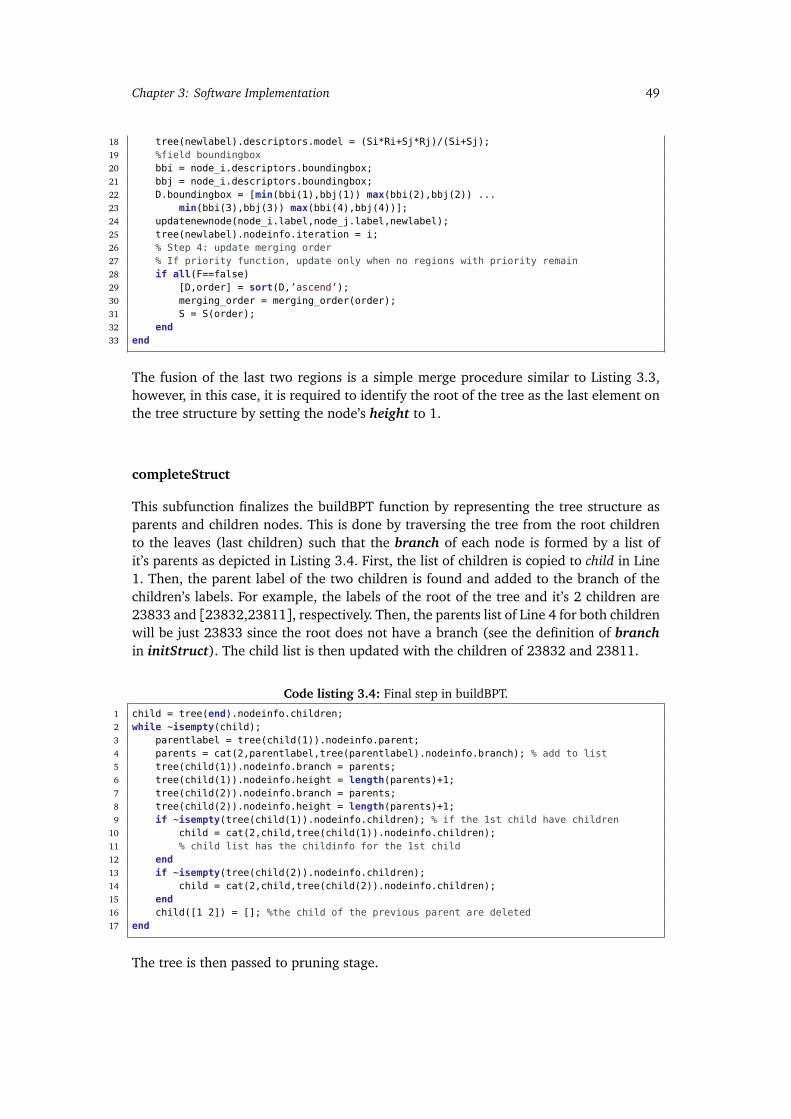
Chapter 3: Software Implementation 49
18 tree(newlabel).descriptors.model = (Si*Ri+Sj*Rj)/(Si+Sj);19 %field boundingbox20 bbi = node_i.descriptors.boundingbox;21 bbj = node_i.descriptors.boundingbox;22 D.boundingbox = [min(bbi(1),bbj(1)) max(bbi(2),bbj(2)) ...23 min(bbi(3),bbj(3)) max(bbi(4),bbj(4))];24 updatenewnode(node_i.label,node_j.label,newlabel);25 tree(newlabel).nodeinfo.iteration = i;26 % Step 4: update merging order27 % If priority function, update only when no regions with priority remain28 if all(F==false)29 [D,order] = sort(D,’ascend’);30 merging_order = merging_order(order);31 S = S(order);32 end33 end
The fusion of the last two regions is a simple merge procedure similar to Listing 3.3,however, in this case, it is required to identify the root of the tree as the last element onthe tree structure by setting the node’s height to 1.
completeStruct
This subfunction finalizes the buildBPT function by representing the tree structure asparents and children nodes. This is done by traversing the tree from the root childrento the leaves (last children) such that the branch of each node is formed by a list ofit’s parents as depicted in Listing 3.4. First, the list of children is copied to child in Line1. Then, the parent label of the two children is found and added to the branch of thechildren’s labels. For example, the labels of the root of the tree and it’s 2 children are23833 and [23832,23811], respectively. Then, the parents list of Line 4 for both childrenwill be just 23833 since the root does not have a branch (see the definition of branchin initStruct). The child list is then updated with the children of 23832 and 23811.
Code listing 3.4: Final step in buildBPT.
1 child = tree(end).nodeinfo.children;2 while ~isempty(child);3 parentlabel = tree(child(1)).nodeinfo.parent;4 parents = cat(2,parentlabel,tree(parentlabel).nodeinfo.branch); % add to list5 tree(child(1)).nodeinfo.branch = parents;6 tree(child(1)).nodeinfo.height = length(parents)+1;7 tree(child(2)).nodeinfo.branch = parents;8 tree(child(2)).nodeinfo.height = length(parents)+1;9 if ~isempty(tree(child(1)).nodeinfo.children); % if the 1st child have children
10 child = cat(2,child,tree(child(1)).nodeinfo.children);11 % child list has the childinfo for the 1st child12 end13 if ~isempty(tree(child(2)).nodeinfo.children);14 child = cat(2,child,tree(child(2)).nodeinfo.children);15 end16 child([1 2]) = []; %the child of the previous parent are deleted17 end
The tree is then passed to pruning stage.
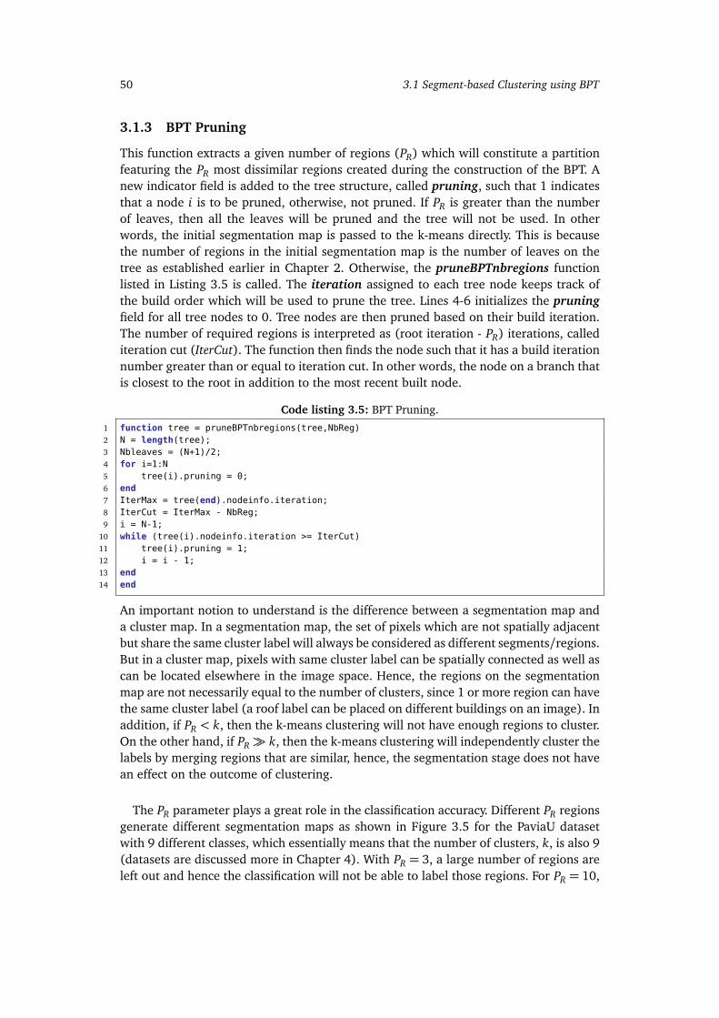
50 3.1 Segment-based Clustering using BPT
3.1.3 BPT Pruning
This function extracts a given number of regions (PR) which will constitute a partitionfeaturing the PR most dissimilar regions created during the construction of the BPT. Anew indicator field is added to the tree structure, called pruning, such that 1 indicatesthat a node i is to be pruned, otherwise, not pruned. If PR is greater than the numberof leaves, then all the leaves will be pruned and the tree will not be used. In otherwords, the initial segmentation map is passed to the k-means directly. This is becausethe number of regions in the initial segmentation map is the number of leaves on thetree as established earlier in Chapter 2. Otherwise, the pruneBPTnbregions functionlisted in Listing 3.5 is called. The iteration assigned to each tree node keeps track ofthe build order which will be used to prune the tree. Lines 4-6 initializes the pruningfield for all tree nodes to 0. Tree nodes are then pruned based on their build iteration.The number of required regions is interpreted as (root iteration - PR) iterations, callediteration cut (IterCut). The function then finds the node such that it has a build iterationnumber greater than or equal to iteration cut. In other words, the node on a branch thatis closest to the root in addition to the most recent built node.
Code listing 3.5: BPT Pruning.
1 function tree = pruneBPTnbregions(tree,NbReg)2 N = length(tree);3 Nbleaves = (N+1)/2;4 for i=1:N5 tree(i).pruning = 0;6 end7 IterMax = tree(end).nodeinfo.iteration;8 IterCut = IterMax - NbReg;9 i = N-1;
10 while (tree(i).nodeinfo.iteration >= IterCut)11 tree(i).pruning = 1;12 i = i - 1;13 end14 end
An important notion to understand is the difference between a segmentation map anda cluster map. In a segmentation map, the set of pixels which are not spatially adjacentbut share the same cluster label will always be considered as different segments/regions.But in a cluster map, pixels with same cluster label can be spatially connected as well ascan be located elsewhere in the image space. Hence, the regions on the segmentationmap are not necessarily equal to the number of clusters, since 1 or more region can havethe same cluster label (a roof label can be placed on different buildings on an image). Inaddition, if PR < k, then the k-means clustering will not have enough regions to cluster.On the other hand, if PR� k, then the k-means clustering will independently cluster thelabels by merging regions that are similar, hence, the segmentation stage does not havean effect on the outcome of clustering.
The PR parameter plays a great role in the classification accuracy. Different PR regionsgenerate different segmentation maps as shown in Figure 3.5 for the PaviaU datasetwith 9 different classes, which essentially means that the number of clusters, k, is also 9(datasets are discussed more in Chapter 4). With PR = 3, a large number of regions areleft out and hence the classification will not be able to label those regions. For PR = 10,
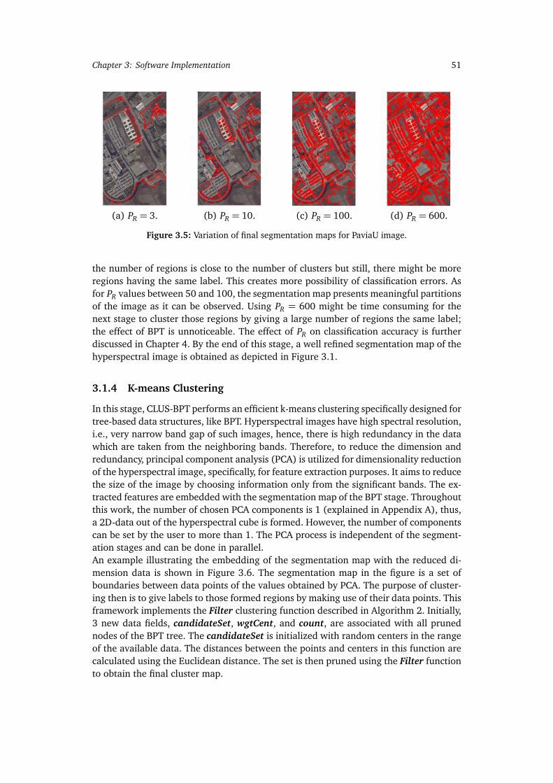
Chapter 3: Software Implementation 51
(a) PR = 3. (b) PR = 10. (c) PR = 100. (d) PR = 600.
Figure 3.5: Variation of final segmentation maps for PaviaU image.
the number of regions is close to the number of clusters but still, there might be moreregions having the same label. This creates more possibility of classification errors. Asfor PR values between 50 and 100, the segmentation map presents meaningful partitionsof the image as it can be observed. Using PR = 600 might be time consuming for thenext stage to cluster those regions by giving a large number of regions the same label;the effect of BPT is unnoticeable. The effect of PR on classification accuracy is furtherdiscussed in Chapter 4. By the end of this stage, a well refined segmentation map of thehyperspectral image is obtained as depicted in Figure 3.1.
3.1.4 K-means Clustering
In this stage, CLUS-BPT performs an efficient k-means clustering specifically designed fortree-based data structures, like BPT. Hyperspectral images have high spectral resolution,i.e., very narrow band gap of such images, hence, there is high redundancy in the datawhich are taken from the neighboring bands. Therefore, to reduce the dimension andredundancy, principal component analysis (PCA) is utilized for dimensionality reductionof the hyperspectral image, specifically, for feature extraction purposes. It aims to reducethe size of the image by choosing information only from the significant bands. The ex-tracted features are embedded with the segmentation map of the BPT stage. Throughoutthis work, the number of chosen PCA components is 1 (explained in Appendix A), thus,a 2D-data out of the hyperspectral cube is formed. However, the number of componentscan be set by the user to more than 1. The PCA process is independent of the segment-ation stages and can be done in parallel.An example illustrating the embedding of the segmentation map with the reduced di-mension data is shown in Figure 3.6. The segmentation map in the figure is a set ofboundaries between data points of the values obtained by PCA. The purpose of cluster-ing then is to give labels to those formed regions by making use of their data points. Thisframework implements the Filter clustering function described in Algorithm 2. Initially,3 new data fields, candidateSet, wgtCent, and count, are associated with all prunednodes of the BPT tree. The candidateSet is initialized with random centers in the rangeof the available data. The distances between the points and centers in this function arecalculated using the Euclidean distance. The set is then pruned using the Filter functionto obtain the final cluster map.

52 3.2 Fast Spectral Clustering
Figure 3.6: PCA and segmentation map embedding example.
3.2 Fast Spectral Clustering
Fast Spectral Clustering (FSC) method is based on incorporating spectral clustering withNyström extension for efficient approximation of the eigenfunction problem. Algorithm5 of section 2.6.5 describes the used FSC method. The framework is illustrated in Figure3.7 and is implemented in this work based on the work of [37] in Python. Using only
Figure 3.7: Flowchart of FSC.
those pixels marked by stars on the input image, a narrow strip of the full W matrix ofEquation 2.21 is computed, shown as the [AB] matrix. Each row contains the affinitiesfrom a sample point to the entire image. The Nyström extension allows one to then dir-ectly approximate the C matrix using the Laplacian matrix. Consequently, approximatethe leading eigenvectors and cluster the image using k-means clustering as described byAlgorithm 5.Listing 3.6 implements FSC on input hyperspectral cube X . The loaded input has thedimensions of pixels × bands. In addition, the function FSC takes m samples and theparameter sigma as inputs. It starts by randomly choosing samples from the input dataof size m and accordingly create two subsets of data. Lines 11 and 12 make use of abuilt-in function to calculate the Euclidean distance between the points. d1 and d2 inLines 19 and 21 correspond to the rows of d in Equation 2.32 of Chapter 2. Matrices Aand B are updated using di,dj,dj+m in Lines 25 and 26. The Laplacian matrix L is thenformed in Line 30. Singular component decomposition built-in function is used to obtainthe eigenvectors of L.Line 34 constitutes the spectral embedding which is done by normalizing each embed-ding vector by first eigenvector (V (:, 1) selects all the rows of the 1st column of V ).Algorithm code from [37] embedding(:, i−1) = V (:, i)./V (:, 1) is used. Finally, the firstk eigenvectors are chosen which are then clustered using Python library built-in k-means
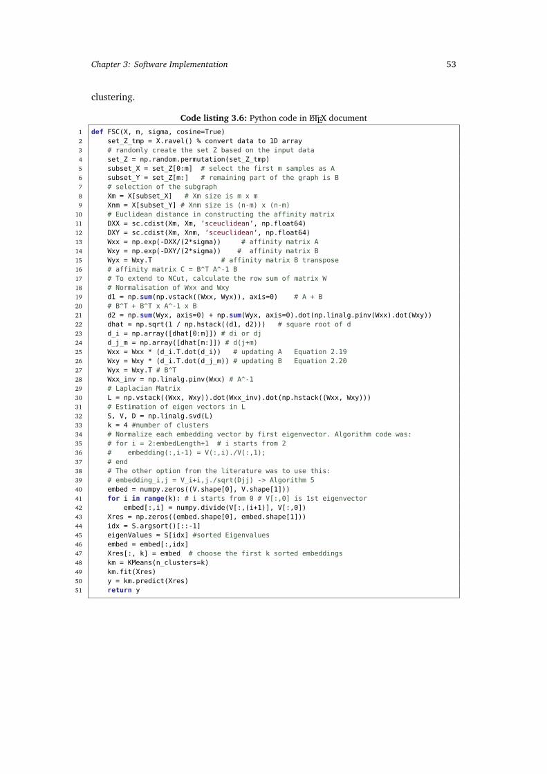
Chapter 3: Software Implementation 53
clustering.
Code listing 3.6: Python code in LATEX document
1 def FSC(X, m, sigma, cosine=True)2 set_Z_tmp = X.ravel() % convert data to 1D array3 # randomly create the set Z based on the input data4 set_Z = np.random.permutation(set_Z_tmp)5 subset_X = set_Z[0:m] # select the first m samples as A6 subset_Y = set_Z[m:] # remaining part of the graph is B7 # selection of the subgraph8 Xm = X[subset_X] # Xm size is m x m9 Xnm = X[subset_Y] # Xnm size is (n-m) x (n-m)
10 # Euclidean distance in constructing the affinity matrix11 DXX = sc.cdist(Xm, Xm, ’sceuclidean’, np.float64)12 DXY = sc.cdist(Xm, Xnm, ’sceuclidean’, np.float64)13 Wxx = np.exp(-DXX/(2*sigma)) # affinity matrix A14 Wxy = np.exp(-DXY/(2*sigma)) # affinity matrix B15 Wyx = Wxy.T # affinity matrix B transpose16 # affinity matrix C = B^T A^-1 B17 # To extend to NCut, calculate the row sum of matrix W18 # Normalisation of Wxx and Wxy19 d1 = np.sum(np.vstack((Wxx, Wyx)), axis=0) # A + B20 # B^T + B^T x A^-1 x B21 d2 = np.sum(Wyx, axis=0) + np.sum(Wyx, axis=0).dot(np.linalg.pinv(Wxx).dot(Wxy))22 dhat = np.sqrt(1 / np.hstack((d1, d2))) # square root of d23 d_i = np.array([dhat[0:m]]) # di or dj24 d_j_m = np.array([dhat[m:]]) # d(j+m)25 Wxx = Wxx * (d_i.T.dot(d_i)) # updating A Equation 2.1926 Wxy = Wxy * (d_i.T.dot(d_j_m)) # updating B Equation 2.2027 Wyx = Wxy.T # B^T28 Wxx_inv = np.linalg.pinv(Wxx) # A^-129 # Laplacian Matrix30 L = np.vstack((Wxx, Wxy)).dot(Wxx_inv).dot(np.hstack((Wxx, Wxy)))31 # Estimation of eigen vectors in L32 S, V, D = np.linalg.svd(L)33 k = 4 #number of clusters34 # Normalize each embedding vector by first eigenvector. Algorithm code was:35 # for i = 2:embedLength+1 # i starts from 236 # embedding(:,i-1) = V(:,i)./V(:,1);37 # end38 # The other option from the literature was to use this:39 # embedding_i,j = V_i+i,j./sqrt(Djj) -> Algorithm 540 embed = numpy.zeros((V.shape[0], V.shape[1]))41 for i in range(k): # i starts from 0 # V[:,0] is 1st eigenvector42 embed[:,i] = numpy.divide(V[:,(i+1)], V[:,0])43 Xres = np.zeros((embed.shape[0], embed.shape[1]))44 idx = S.argsort()[::-1]45 eigenValues = S[idx] #sorted Eigenvalues46 embed = embed[:,idx]47 Xres[:, k] = embed # choose the first k sorted embeddings48 km = KMeans(n_clusters=k)49 km.fit(Xres)50 y = km.predict(Xres)51 return y

Chapter 4
Software Results
In this chapter, clustering performance of the segment-based clustering using BinaryPartition Trees framework (described in section 3.1) and the Fast Spectral Clustering(described in section 3.2) is tested and compared with one other state-of-the-art clus-tering method. The experiments are performed on eight different hyperspectral images.To evaluate their performance, metrics such as Normalized Mutual Information (NMI)and Purity are used. This analysis serves as a basis for the algorithm choice for FPGAimplementation.
4.1 Software Results for CLUS-BPT and FSC
To assess the effectiveness of the CLUS-BPT and the FSC method, it is compared with thesegment-based projected clustering using mutual nearest neighbour (PCMNN) method[18] discussed earlier in section 2.3.2. Note that for Fast Spectral Clustering (FSC), thevalues mentioned are the reported ones from the HSI spectral clustering implementa-tion by [12] since it provided more accurate results than the implementation of Listing3.6 and hence, more challenging results.Further, to test the performance of the proposed frameworks, evaluation is carried onHSI datasets, and then several useful analysis are discussed. The experiments wereran under the same environment: Intel(R) Core(TM) i7-5930K CPU, 3.50 GHz, 64 GBmemory, Windows 10 OS, Matlab version R2019a and Python 3.7.3.
4.2 Experimental Datasets
Experiments were conducted on eight widely used hyperspectral datasets.
• Salinas scene was collected by the 224-band AVIRIS (Airborne Visible/InfraredImaging Spectrometer) sensor over Salinas Valley, California, and is character-ized by high spatial resolution (3.7-meter pixels). Salinas covers 512 lines by 217samples at as scale of 512× 217. Salinas ground truth contains 16 classes.
• Salinas-A is a small subscene of Salinas image and it comprises 86×83 pixels loc-ated within the same scene as Salinas at [samples, lines] = [591–676, 158–240].It includes vegetables, bare soils, and vineyard fields. Salinas-A ground truth con-tains 6 classes.
55
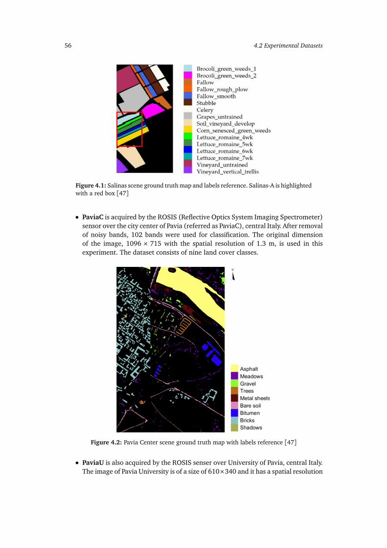
56 4.2 Experimental Datasets
Figure 4.1: Salinas scene ground truth map and labels reference. Salinas-A is highlightedwith a red box [47]
• PaviaC is acquired by the ROSIS (Reflective Optics System Imaging Spectrometer)sensor over the city center of Pavia (referred as PaviaC), central Italy. After removalof noisy bands, 102 bands were used for classification. The original dimensionof the image, 1096 × 715 with the spatial resolution of 1.3 m, is used in thisexperiment. The dataset consists of nine land cover classes.
Figure 4.2: Pavia Center scene ground truth map with labels reference [47]
• PaviaU is also acquired by the ROSIS senser over University of Pavia, central Italy.The image of Pavia University is of a size of 610×340 and it has a spatial resolution
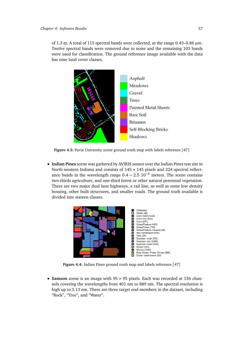
Chapter 4: Software Results 57
of 1.3 m. A total of 115 spectral bands were collected, at the range 0.43–0.86 µm.Twelve spectral bands were removed due to noise and the remaining 103 bandswere used for classification. The ground reference image available with the datahas nine land cover classes.
Figure 4.3: Pavia University scene ground truth map with labels reference [47]
• Indian Pines scene was gathered by AVIRIS sensor over the Indian Pines test site inNorth-western Indiana and consists of 145× 145 pixels and 224 spectral reflect-ance bands in the wavelength range 0.4 − 2.5 10−6 meters. The scene containstwo-thirds agriculture, and one-third forest or other natural perennial vegetation.There are two major dual lane highways, a rail line, as well as some low densityhousing, other built structures, and smaller roads. The ground truth available isdivided into sixteen classes.
Figure 4.4: Indian Pines ground truth map and labels reference [47]
• Samson scene is an image with 95× 95 pixels. Each was recorded at 156 chan-nels covering the wavelengths from 401 nm to 889 nm. The spectral resolution ishigh up to 3.13 nm. There are three target end-members in the dataset, including“Rock”, “Tree”, and “Water”.
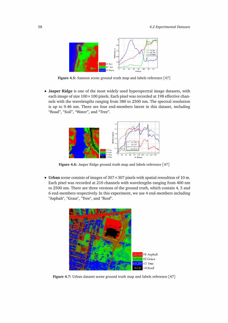
58 4.2 Experimental Datasets
Figure 4.5: Samson scene ground truth map and labels reference [47]
• Jasper Ridge is one of the most widely used hyperspectral image datasets, witheach image of size 100×100 pixels. Each pixel was recorded at 198 effective chan-nels with the wavelengths ranging from 380 to 2500 nm. The spectral resolutionis up to 9.46 nm. There are four end-members latent in this dataset, including“Road”, “Soil”, “Water”, and “Tree”.
Figure 4.6: Jasper Ridge ground truth map and labels reference [47]
• Urban scene consists of images of 307×307 pixels with spatial resoultion of 10 m.Each pixel was recorded at 210 channels with wavelengths ranging from 400 nmto 2500 nm. There are three versions of the ground truth, which contain 4, 5 and6 end-members respectively. In this experiment, we use 4 end-members including"Asphalt", "Grass", "Tree", and "Roof".
Figure 4.7: Urban dataset scene ground truth map and labels reference [47]
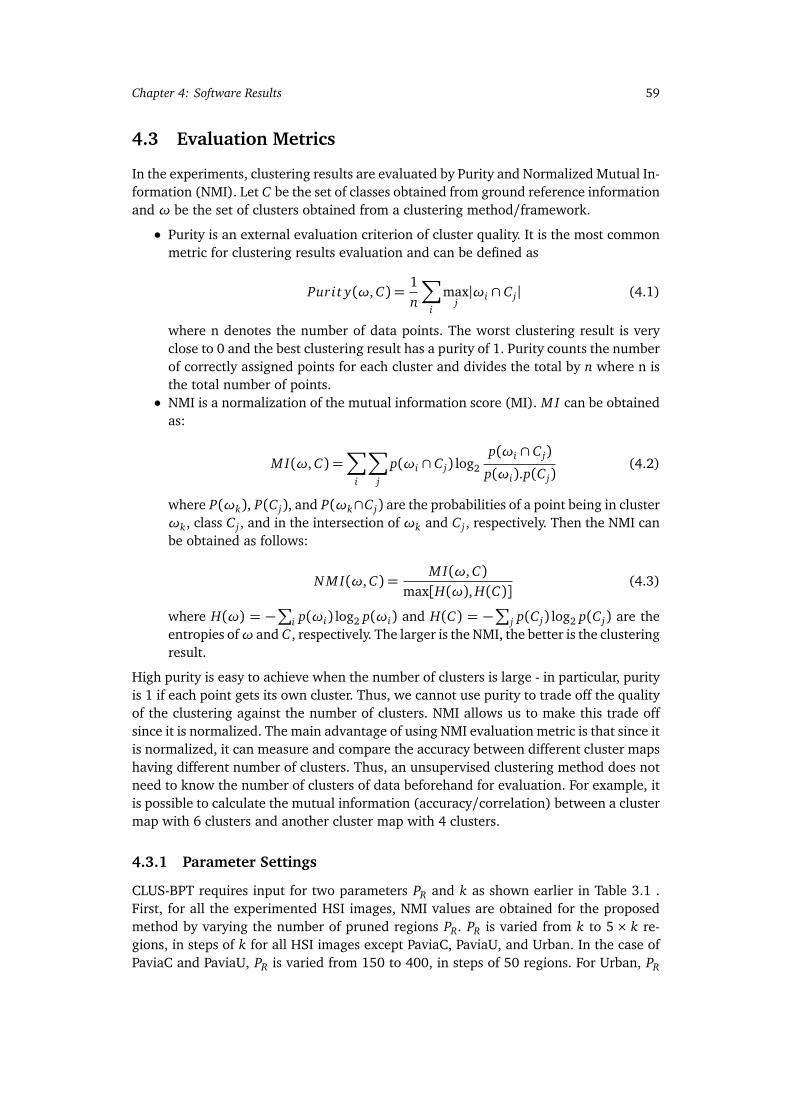
Chapter 4: Software Results 59
4.3 Evaluation Metrics
In the experiments, clustering results are evaluated by Purity and Normalized Mutual In-formation (NMI). Let C be the set of classes obtained from ground reference informationand ω be the set of clusters obtained from a clustering method/framework.
• Purity is an external evaluation criterion of cluster quality. It is the most commonmetric for clustering results evaluation and can be defined as
Puri t y(ω, C) =1n
∑
i
maxj|ωi ∩ C j| (4.1)
where n denotes the number of data points. The worst clustering result is veryclose to 0 and the best clustering result has a purity of 1. Purity counts the numberof correctly assigned points for each cluster and divides the total by n where n isthe total number of points.
• NMI is a normalization of the mutual information score (MI). M I can be obtainedas:
M I(ω, C) =∑
i
∑
j
p(ωi ∩ C j) log2
p(ωi ∩ C j)
p(ωi).p(C j)(4.2)
where P(ωk), P(C j), and P(ωk∩C j) are the probabilities of a point being in clusterωk, class C j , and in the intersection of ωk and C j , respectively. Then the NMI canbe obtained as follows:
N M I(ω, C) =M I(ω, C)
max[H(ω), H(C)](4.3)
where H(ω) = −∑
i p(ωi) log2 p(ωi) and H(C) = −∑
j p(C j) log2 p(C j) are theentropies ofω and C , respectively. The larger is the NMI, the better is the clusteringresult.
High purity is easy to achieve when the number of clusters is large - in particular, purityis 1 if each point gets its own cluster. Thus, we cannot use purity to trade off the qualityof the clustering against the number of clusters. NMI allows us to make this trade offsince it is normalized. The main advantage of using NMI evaluation metric is that since itis normalized, it can measure and compare the accuracy between different cluster mapshaving different number of clusters. Thus, an unsupervised clustering method does notneed to know the number of clusters of data beforehand for evaluation. For example, itis possible to calculate the mutual information (accuracy/correlation) between a clustermap with 6 clusters and another cluster map with 4 clusters.
4.3.1 Parameter Settings
CLUS-BPT requires input for two parameters PR and k as shown earlier in Table 3.1 .First, for all the experimented HSI images, NMI values are obtained for the proposedmethod by varying the number of pruned regions PR. PR is varied from k to 5 × k re-gions, in steps of k for all HSI images except PaviaC, PaviaU, and Urban. In the case ofPaviaC and PaviaU, PR is varied from 150 to 400, in steps of 50 regions. For Urban, PR
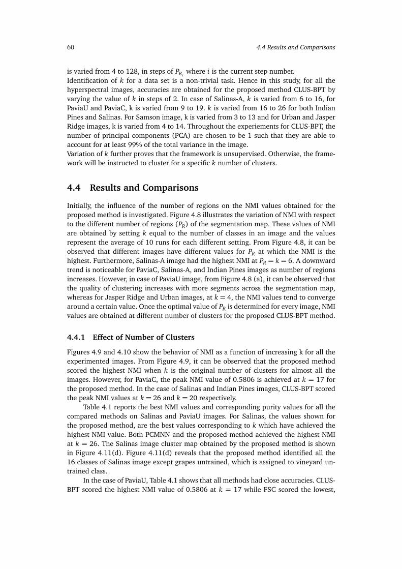
60 4.4 Results and Comparisons
is varied from 4 to 128, in steps of PRiwhere i is the current step number.
Identification of k for a data set is a non-trivial task. Hence in this study, for all thehyperspectral images, accuracies are obtained for the proposed method CLUS-BPT byvarying the value of k in steps of 2. In case of Salinas-A, k is varied from 6 to 16, forPaviaU and PaviaC, k is varied from 9 to 19. k is varied from 16 to 26 for both IndianPines and Salinas. For Samson image, k is varied from 3 to 13 and for Urban and JasperRidge images, k is varied from 4 to 14. Throughout the experiements for CLUS-BPT, thenumber of principal components (PCA) are chosen to be 1 such that they are able toaccount for at least 99% of the total variance in the image.Variation of k further proves that the framework is unsupervised. Otherwise, the frame-work will be instructed to cluster for a specific k number of clusters.
4.4 Results and Comparisons
Initially, the influence of the number of regions on the NMI values obtained for theproposed method is investigated. Figure 4.8 illustrates the variation of NMI with respectto the different number of regions (PR) of the segmentation map. These values of NMIare obtained by setting k equal to the number of classes in an image and the valuesrepresent the average of 10 runs for each different setting. From Figure 4.8, it can beobserved that different images have different values for PR at which the NMI is thehighest. Furthermore, Salinas-A image had the highest NMI at PR = k = 6. A downwardtrend is noticeable for PaviaC, Salinas-A, and Indian Pines images as number of regionsincreases. However, in case of PaviaU image, from Figure 4.8 (a), it can be observed thatthe quality of clustering increases with more segments across the segmentation map,whereas for Jasper Ridge and Urban images, at k = 4, the NMI values tend to convergearound a certain value. Once the optimal value of PR is determined for every image, NMIvalues are obtained at different number of clusters for the proposed CLUS-BPT method.
4.4.1 Effect of Number of Clusters
Figures 4.9 and 4.10 show the behavior of NMI as a function of increasing k for all theexperimented images. From Figure 4.9, it can be observed that the proposed methodscored the highest NMI when k is the original number of clusters for almost all theimages. However, for PaviaC, the peak NMI value of 0.5806 is achieved at k = 17 forthe proposed method. In the case of Salinas and Indian Pines images, CLUS-BPT scoredthe peak NMI values at k = 26 and k = 20 respectively.
Table 4.1 reports the best NMI values and corresponding purity values for all thecompared methods on Salinas and PaviaU images. For Salinas, the values shown forthe proposed method, are the best values corresponding to k which have achieved thehighest NMI value. Both PCMNN and the proposed method achieved the highest NMIat k = 26. The Salinas image cluster map obtained by the proposed method is shownin Figure 4.11(d). Figure 4.11(d) reveals that the proposed method identified all the16 classes of Salinas image except grapes untrained, which is assigned to vineyard un-trained class.
In the case of PaviaU, Table 4.1 shows that all methods had close accuracies. CLUS-BPT scored the highest NMI value of 0.5806 at k = 17 while FSC scored the lowest,
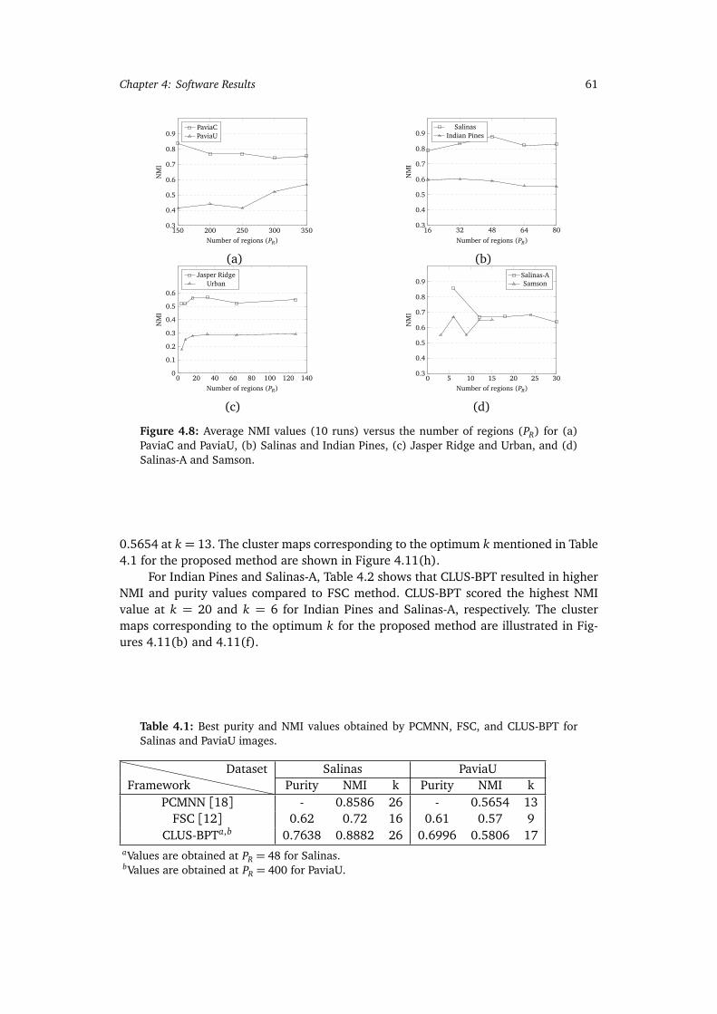
Chapter 4: Software Results 61
150 200 250 300 3500.3
0.4
0.5
0.6
0.7
0.8
0.9
Number of regions (PR)
NM
I
PaviaCPaviaU
(a)
16 32 48 64 800.3
0.4
0.5
0.6
0.7
0.8
0.9
Number of regions (PR)
NM
I
SalinasIndian Pines
(b)
0 20 40 60 80 100 120 1400
0.1
0.2
0.3
0.4
0.5
0.6
Number of regions (PR)
NM
I
Jasper RidgeUrban
(c)
0 5 10 15 20 25 300.3
0.4
0.5
0.6
0.7
0.8
0.9
Number of regions (PR)
NM
I
Salinas-ASamson
(d)
Figure 4.8: Average NMI values (10 runs) versus the number of regions (PR) for (a)PaviaC and PaviaU, (b) Salinas and Indian Pines, (c) Jasper Ridge and Urban, and (d)Salinas-A and Samson.
0.5654 at k = 13. The cluster maps corresponding to the optimum k mentioned in Table4.1 for the proposed method are shown in Figure 4.11(h).
For Indian Pines and Salinas-A, Table 4.2 shows that CLUS-BPT resulted in higherNMI and purity values compared to FSC method. CLUS-BPT scored the highest NMIvalue at k = 20 and k = 6 for Indian Pines and Salinas-A, respectively. The clustermaps corresponding to the optimum k for the proposed method are illustrated in Fig-ures 4.11(b) and 4.11(f).
Table 4.1: Best purity and NMI values obtained by PCMNN, FSC, and CLUS-BPT forSalinas and PaviaU images.
FrameworkDataset Salinas PaviaU
Purity NMI k Purity NMI kPCMNN [18] - 0.8586 26 - 0.5654 13
FSC [12] 0.62 0.72 16 0.61 0.57 9CLUS-BPTa,b 0.7638 0.8882 26 0.6996 0.5806 17
aValues are obtained at PR = 48 for Salinas.bValues are obtained at PR = 400 for PaviaU.
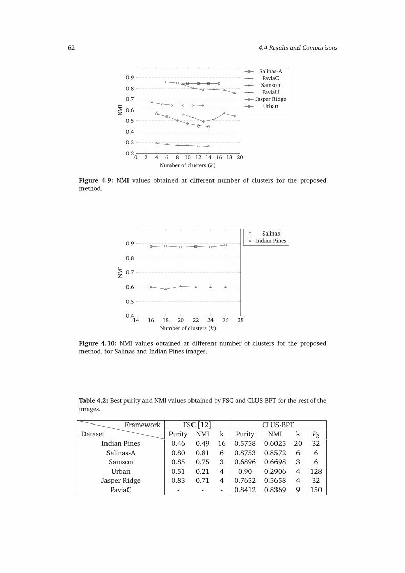
62 4.4 Results and Comparisons
0 2 4 6 8 10 12 14 16 18 200.2
0.3
0.4
0.5
0.6
0.7
0.8
0.9
Number of clusters (k)
NM
I
Salinas-APaviaCSamsonPaviaU
Jasper RidgeUrban
Figure 4.9: NMI values obtained at different number of clusters for the proposedmethod.
14 16 18 20 22 24 26 280.4
0.5
0.6
0.7
0.8
0.9
Number of clusters (k)
NM
I
SalinasIndian Pines
Figure 4.10: NMI values obtained at different number of clusters for the proposedmethod, for Salinas and Indian Pines images.
Table 4.2: Best purity and NMI values obtained by FSC and CLUS-BPT for the rest of theimages.
DatasetFramework FSC [12] CLUS-BPT
Purity NMI k Purity NMI k PR
Indian Pines 0.46 0.49 16 0.5758 0.6025 20 32Salinas-A 0.80 0.81 6 0.8753 0.8572 6 6Samson 0.85 0.75 3 0.6896 0.6698 3 6Urban 0.51 0.21 4 0.90 0.2906 4 128
Jasper Ridge 0.83 0.71 4 0.7652 0.5658 4 32PaviaC - - - 0.8412 0.8369 9 150
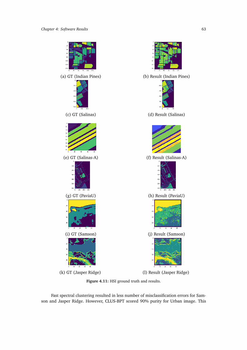
Chapter 4: Software Results 63
(a) GT (Indian Pines) (b) Result (Indian Pines)
(c) GT (Salinas) (d) Result (Salinas)
(e) GT (Salinas-A) (f) Result (Salinas-A)
(g) GT (PaviaU) (h) Result (PaviaU)
(i) GT (Samson) (j) Result (Samson)
(k) GT (Jasper Ridge) (l) Result (Jasper Ridge)
Figure 4.11: HSI ground truth and results.
Fast spectral clustering resulted in less number of misclassification errors for Sam-son and Jasper Ridge. However, CLUS-BPT scored 90% purity for Urban image. This
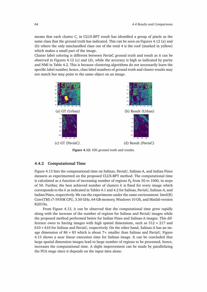
64 4.4 Results and Comparisons
means that each cluster Ci in CLUS-BPT result has identified a group of pixels as thesame class that the ground truth has indicated. This can be seen on Figures 4.12 (a) and(b) where the only misclassified class out of the total 4 is the roof (marked in yellow)which makes a small part of the image.Cluster label coloring is different between PaviaC ground truth and result as it can beobserved in Figures 4.12 (c) and (d), while the accuracy is high as indicated by purityand NMI in Table 4.2. This is because clustering algorithms do not necessarily learn thespecific label number, hence, class label numbers of ground truth and cluster results maynot match but may point to the same object on an image.
(a) GT (Urban) (b) Result (Urban)
(c) GT (PaviaC) (d) Result (PaviaC)
Figure 4.12: HSI ground truth and results.
4.4.2 Computational Time
Figure 4.13 lists the computational time on Salinas, PaviaU, Salinas-A, and Indian Pinesdatasets as experimented on the proposed CLUS-BPT method. The computational timeis calculated as a function of increasing number of regions PR from 50 to 1000, in stepsof 50. Further, the best achieved number of clusters k is fixed for every image whichcorresponds to the k as indicated in Tables 4.1 and 4.2 for Salinas, PaviaU, Salinas-A, andIndian Pines, respectively. We ran the experiments under the same environment: Intel(R)Core(TM) i7-5930K CPU, 3.50 GHz, 64 GB memory, Windows 10 OS, and Matlab versionR2019a.
From Figure 4.13, it can be observed that the computational time grew rapidlyalong with the increase of the number of regions for Salinas and PaviaU images whilethe proposed method performed better for Indian Pines and Salinas-A images. This dif-ference owes to having images with high spatial dimensions, such as 512 × 217 and610×610 for Salinas and PaviaU, respectively. On the other hand, Salinas-A has an im-age dimension of 86 × 83 which is about 7× smaller than Salinas and PaviaU. Figure4.13 shows a near linear execution time for Salinas image. It can be concluded thatlarge spatial dimension images lead to large number of regions to be processed, hence,increases the computational time. A slight improvement can be made by parallelizingthe PCA stage since it depends on the input data alone.
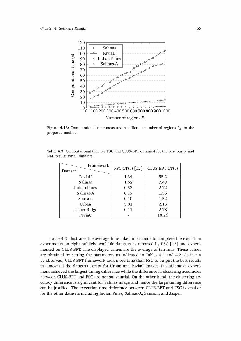
Chapter 4: Software Results 65
0 100 200 300 400 500 600 700 800 9001,0000
102030405060708090
100110120
Number of regions PR
Com
puta
tion
alti
me
(s)
SalinasPaviaU
Indian PinesSalinas-A
Figure 4.13: Computational time measured at different number of regions PR for theproposed method.
Table 4.3: Computational time for FSC and CLUS-BPT obtained for the best purity andNMI results for all datasets.
DatasetFramework
FSC CT(s) [12] CLUS-BPT CT(s)
PaviaU 1.34 58.2Salinas 1.62 7.48
Indian Pines 0.53 2.72Salinas-A 0.17 1.56Samson 0.10 1.52Urban 3.01 2.15
Jasper Ridge 0.11 2.78PaviaC - 18.26
Table 4.3 illustrates the average time taken in seconds to complete the executionexperiments on eight publicly available datasets as reported by FSC [12] and experi-mented on CLUS-BPT. The displayed values are the average of ten runs. These valuesare obtained by setting the parameters as indicated in Tables 4.1 and 4.2. As it canbe observed, CLUS-BPT framework took more time than FSC to output the best resultsin almost all the datasets except for Urban and PaviaC images. PaviaU image experi-ment achieved the largest timing difference while the difference in clustering accuraciesbetween CLUS-BPT and FSC are not substantial. On the other hand, the clustering ac-curacy difference is significant for Salinas image and hence the large timing differencecan be justified. The execution time difference between CLUS-BPT and FSC is smallerfor the other datasets including Indian Pines, Salinas-A, Samson, and Jasper.

66 4.5 Algorithm Choice
4.5 Algorithm Choice
In order to choose the adequate algorithm for FPGA implementation, experiments ofboth methods were carried out in this chapter on eight different HSI datasets. Evaluationperformance included purity, NMI, and computational time. According to the followingobservations made on Tables 4.1, 4.2, and 4.3, the Fast Spectral Clustering (FSC) methodis chosen for FPGA Implementation:
• Fast Spectral Clustering (FSC) execution time on almost all datasets is much lowerthan that of CLUS-BPT. On some datasets, the computational time is near real-time.
• Classification performance of both methods are quite comparable with slight pos-itive difference for CLUS-BPT. Hence, the choice is a trade-off between speed andaccuracy.
• CLUS-BPT involves a long list of components including watershed segmentation,BPT construction, BPT pruning, PCA, and filtering algorithm for k-means cluster-ing. While on the other hand, FSC uses less number of components and also hasthe advantage of deploying numerical approximations.
• In addition, FSC involves matrix processing functions which has been implemen-ted on FPGAs in literature.
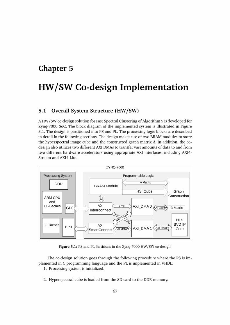
Chapter 5
HW/SW Co-design Implementation
5.1 Overall System Structure (HW/SW)
A HW/SW co-design solution for Fast Spectral Clustering of Algorithm 5 is developed forZynq-7000 SoC. The block diagram of the implemented system is illustrated in Figure5.1. The design is partitioned into PS and PL. The processing logic blocks are describedin detail in the following sections. The design makes use of two BRAM modules to storethe hyperspectral image cube and the constructed graph matrix A. In addition, the co-design also utilizes two different AXI DMAs to transfer vast amounts of data to and fromtwo different hardware accelerators using appropriate AXI interfaces, including AXI4-Stream and AXI4-Lite.
Figure 5.1: PS and PL Partitions in the Zynq-7000 HW/SW co-design.
The co-design solution goes through the following procedure where the PS is im-plemented in C programming language and the PL is implemented in VHDL:
1. Processing system is initialized.
2. Hyperspectral cube is loaded from the SD card to the DDR memory.
67

68 5.1 Overall System Structure (HW/SW)
3. BRAM module and 2 AXI_DMAs transfers are configured via AXI-lite register filethrough AXI_Interconnect.
4. HSI cube is written to BRAM by making use of a General Purpose AXI master port(GP0) in the Zynq PS.
5. Graph Construction module reads the HSI data band per pixel, processes the af-finity matrices A and writes it back to the BRAM. Meanwhile, matrix B is beingcomputed and streamed through AXI_DMA_0.
6. Matrices A and B are read by the PS and saved in DDR memory.
7. The PS forms the Laplacian matrix as means of this expression
�
AB
�
A−1�
A B�
by
making use of the necessary matrix multiplication and matrix inverse.
8. The High Performance (HP0) port of Zynq PS connected to the external DDRmemory and is used along with AXI_DMA_1 to stream the Laplacian matrix tothe high-level synthesis module of SVD.
9. The eigenvalue and eigenvector decompositions computed by SVD core are streamedback to the PS.
10. The PS C code sorts the eigenvalues and the corresponding eigenvectors. In addi-tion, it clusters the sorted eigenvectors using K-means clustering.
11. Finally, clustering results are written to the SD card. Results can be plotted usingMATLAB/Python.
Before loading HSI cube from the SD card to the DDR memory, the design requiresdata preprocessing, which is done by reducing the HSI spectral bands dimension to 16using PCA on MATLAB. Generic data parameters are kept consistent throughout theproject and are designed to be modular such that the generic parameters control thedesign size. Table 5.1 shows the generic parameters, their description, and examplevalues used throughout the HW/SW co-design modules. The default values for pixeldimensions are based on the reduced Salinas-A dataset.
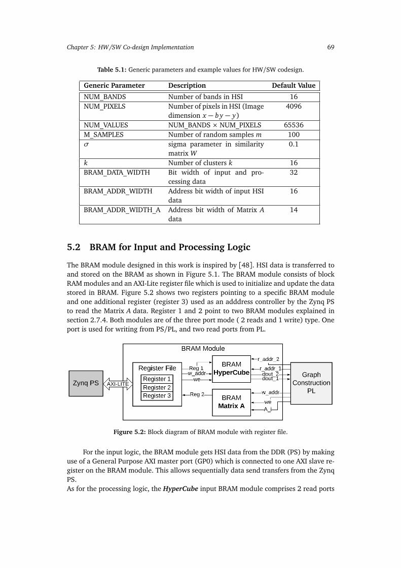
Chapter 5: HW/SW Co-design Implementation 69
Table 5.1: Generic parameters and example values for HW/SW codesign.
Generic Parameter Description Default Value
NUM_BANDS Number of bands in HSI 16NUM_PIXELS Number of pixels in HSI (Image
dimension x − b y − y)4096
NUM_VALUES NUM_BANDS × NUM_PIXELS 65536M_SAMPLES Number of random samples m 100σ sigma parameter in similarity
matrix W0.1
k Number of clusters k 16BRAM_DATA_WIDTH Bit width of input and pro-
cessing data32
BRAM_ADDR_WIDTH Address bit width of input HSIdata
16
BRAM_ADDR_WIDTH_A Address bit width of Matrix Adata
14
5.2 BRAM for Input and Processing Logic
The BRAM module designed in this work is inspired by [48]. HSI data is transferred toand stored on the BRAM as shown in Figure 5.1. The BRAM module consists of blockRAM modules and an AXI-Lite register file which is used to initialize and update the datastored in BRAM. Figure 5.2 shows two registers pointing to a specific BRAM moduleand one additional register (register 3) used as an adddress controller by the Zynq PSto read the Matrix A data. Register 1 and 2 point to two BRAM modules explained insection 2.7.4. Both modules are of the three port mode ( 2 reads and 1 write) type. Oneport is used for writing from PS/PL, and two read ports from PL.
Figure 5.2: Block diagram of BRAM module with register file.
For the input logic, the BRAM module gets HSI data from the DDR (PS) by makinguse of a General Purpose AXI master port (GP0) which is connected to one AXI slave re-gister on the BRAM module. This allows sequentially data send transfers from the ZynqPS.As for the processing logic, the HyperCube input BRAM module comprises 2 read ports
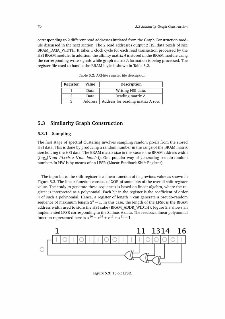
70 5.3 Similarity Graph Construction
corresponding to 2 different read addresses initiated from the Graph Construction mod-ule discussed in the next section. The 2 read addresses output 2 HSI data pixels of sizeBRAM_DATA_WIDTH. It takes 1 clock cycle for each read transaction processed by theHSI BRAM module. In addition, the affinity matrix A is stored in the BRAM module usingthe corresponding write signals while graph matrix A formation is being processed. Theregister file used to handle the BRAM logic is shown in Table 5.2.
Table 5.2: AXI-lite register file description.
Register Value Description
1 Data Writing HSI data.2 Data Reading matrix A.3 Address Address for reading matrix A row.
5.3 Similarity Graph Construction
5.3.1 Sampling
The first stage of spectral clustering involves sampling random pixels from the storedHSI data. This is done by producing a random number in the range of the BRAM matrixsize holding the HSI data. The BRAM matrix size in this case is the BRAM address width(log2(Num_Pixels × Num_bands)). One popular way of generating pseudo-randomnumbers in HW is by means of an LFSR (Linear-Feedback Shift Register).
The input bit to the shift register is a linear function of its previous value as shown inFigure 5.3. The linear function consists of XOR of some bits of the overall shift registervalue. The study to generate these sequences is based on linear algebra, where the re-gister is interpreted as a polynomial. Each bit in the register is the coefficient of ordern of such a polynomial. Hence, a register of length n can generate a pseudo-randomsequence of maximum length 2n − 1. In this case, the length of the LFSR is the BRAMaddress width used to store the HSI cube (BRAM_ADDR_WIDTH). Figure 5.3 shows animplemented LFSR corresponding to the Salinas-A data. The feedback linear polynomialfunction represented here is x16 + x14 + x13 + x11 + 1.
Figure 5.3: 16-bit LFSR.
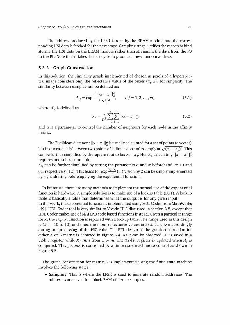
Chapter 5: HW/SW Co-design Implementation 71
The address produced by the LFSR is read by the BRAM module and the corres-ponding HSI data is fetched for the next stage. Sampling stage justifies the reason behindstoring the HSI data on the BRAM module rather than streaming the data from the PSto the PL. Note that it takes 1 clock cycle to produce a new random address.
5.3.2 Graph Construction
In this solution, the similarity graph implemented of chosen m pixels of a hyperspec-tral image considers only the reflectance value of the pixels (x i , x j) for simplicity. Thesimilarity between samples can be defined as:
Ai j = exp−||x i − x j||22
2ασx2 , i, j = 1,2, . . . , m, (5.1)
where σx is defined as
σx =1n2
n∑
i=1
n∑
j=1
||x i − x j||22. (5.2)
and α is a parameter to control the number of neighbors for each node in the affinitymatrix.
The Euclidean distance : ||x i−x j||22 is usually calculated for a set of points (a vector)but in our case, it is between two points of 1 dimension and is simply=
Æ
(x i − x j)2. Thiscan be further simplified by the square root to be: x i − x j . Hence, calculating ||x i − x j||22requires one subtraction unit.Ai j can be further simplified by setting the parameters α and σ beforehand, to 10 and
0.1 respectively [12]. This leads to (expx j−x i
2 ). Division by 2 can be simply implementedby right shifting before applying the exponential function.
In literature, there are many methods to implement the normal use of the exponentialfunction in hardware. A simple solution is to make use of a lookup table (LUT). A lookuptable is basically a table that determines what the output is for any given input.In this work, the exponential function is implemented using HDL Coder from MathWorks[49]. HDL Coder tool is very similar to Vivado HLS discussed in section 2.8, except thatHDL Coder makes use of MATLAB code based functions instead. Given a particular rangefor x , the ex p(x) function is replaced with a lookup table. The range used in this designis (x : −10 to 10) and thus, the input reflectance values are scaled down accordinglyduring pre-processing of the HSI cube. The RTL design of the graph construction foreither A or B matrix is depicted in Figure 5.4. As it can be observed, X i is saved in a32-bit register while X j runs from 1 to m. The 32-bit register is updated when Ai iscomputed. This process is controlled by a finite state machine to control as shown inFigure 5.5.
The graph construction for matrix A is implemented using the finite state machineinvolves the following states:
• Sampling: This is where the LFSR is used to generate random addresses. Theaddresses are saved in a block RAM of size m samples.
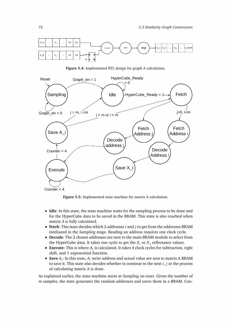
72 5.3 Similarity Graph Construction
Figure 5.4: Implemented RTL design for graph A calculation.
Figure 5.5: Implemented state machine for matrix A calculation.
• Idle: In this state, the state machine waits for the sampling process to be done andfor the HyperCube data to be saved in the BRAM. This state is also reached whenmatrix A is fully calculated.
• Fetch: This state decides which 2 addresses i and j to get from the addresses BRAMinitiliazed in the Sampling stage. Reading an address requires one clock cycle.
• Decode: The 2 chosen addresses are sent to the main BRAM module to select fromthe HyperCube data. It takes one cycle to get the X i or X j reflectance values.
• Execute: This is where Ai is calculated. It takes 4 clock cycles for subtraction, rightshift, and 1 exponential function.
• Save Ai: In this state, Ai write address and actual value are sent to matrix A BRAMto save it. This state also decides whether to continue to the next i, j or the processof calculating matrix A is done.
As explained earlier, the state machine starts at Sampling on reset. Given the number ofm samples, the state generates the random addresses and saves them in a BRAM. Con-

Chapter 5: HW/SW Co-design Implementation 73
currently, the BRAM module accepts the input HyberCube data sent from the Zynq PS,since the Sampling state does not depend on the input data rather, the size of the datawhich is set as a generic parameter (NUM_VALUES). Graph_en signals the Idle state thatthe random number generation is done and saved. Once the input data is loaded on theHSI BRAM, HyperCube_Ready signals the Fetch state that the full input data is capturedand ready for processing.
Fetch state is directly reading from the BRAM of sample addresses. Counters i and jare pointers corresponding to the addresses of the BRAM sample addresses. However,read access is done per 1 instruction for either i or j and not concurrently. The idea ofthe coming states is to fix an address i and increment address j until m and then incre-ment i for every j = m reached until i = m.
If it is a new round/loop, then j = 0 and a new address i is fetched. The fetched ad-dress is sent to the BRAM to decode, which takes 1 clock cycle equivalent to the Decodestate. Meanwhile, address j is fetched from the sample addresses BRAM. Next, the statemachine goes to another Decode state to decode the j address. Meanwhile, the decodedX i value is saved in a 32-bit register for usage in the coming loop. If it is not a newround/loop, then j 6= 0 and a similar Fetch, Decode process applies for address j.
The Execute state already has the saved X i as one of the operands of the subtractionunit. After calculation of Ai , the value is written to the matrix A BRAM, which can bealso read by the Zynq PS. The Save Ai state goes to Fetch if the calculation is not done(i 6= m), otherwise, it goes to the Idle state.
The critical path for the matrix A calculation is 9m2 + 1 with 1 subtraction unit, 1 LUT,and 1 right shift operation. m sampling clock cycles take place while HyperCube datainput is being written to the BRAM so it is not considered as part of the critical path. The+1 represents the first Idle state. Fetch and Decode states take 1 clock cycle each and 1clock cycle for saving X i in a register. Furthermore, the critical path for 1 loop is 9 clockcycles with the longest path: Fetch→ Fetch Address i→ Decode Address i→ Save X i →Execute→ Save Ai .
Matrix B calculation follows a similar RTL implementation as in Figure 5.4 as well asthe finite state machine in Figure 5.5. However, for the RTL implementation, i : 0→ mand j : 0→ (n−m). Hence, resource-wise, matrix B computation requires the same setof resources as matrix A.As for the FSM, matrix B calculation differs in the Save Bi stage. The size of B ism× (n−m) where n� m = 128× (65536− 128) = 8372224 values, using the genericparameters. Hence, it is expensive, resource-wise, to store matrix B on the BRAM. In-stead, it is saved in the DDR memory on Zynq PS. Master Output module, adapted from[48], streams the calculated matrix Bi to Zynq PS by communicating with AXI_DMA_0.The output module acts as an AXI stream master interface setting the different AXI4-Stream channels TDATA and TLAST. Moreover, the AXI stream on the DMA is connectedto a high performance AXI slave interface which provides a high bandwidth data-pathfrom the master modules (such as Master Output) in PL to the DDR on Zynq PS.

74 5.3 Similarity Graph Construction
Laplacian Matrix Formation
To this end, Zynq PS has matrix B stored in the DDR memory. Matrix A can be readfrom the BRAM register address 0. Both matrices A and B are used to form the Laplacianmatrix L on Zynq PS as in Algorithm 5. The matrix L size is expected to be n− b y − nwhere n= 65536 is NUM_VALUES. Hence, a total number of 65536x65536 values willhave to be streamed to the HLS SVD IP core to compute the eigenvalue and eigenvectordecomposition and send back to the PS three matrices of size n− b y−n each. This com-prises large utilization of BRAM resources used to store partial results of SVD (discussedin the next section). Consequently, the design may require to use BRAM resources morethan the resource limit available on the Zynq-7000 platform. Thus, a work-around is tocompute the eigenvalue and eigenvector of a smaller size matrix.
[37] found that if A is positive definite, then we can solve for the approximate eigen-vectors in one step. Let A
12 denote the symmetric positive definite square root of A, then,
define Q:
Q = A+ A−12 BBT A−
12 , (5.3)
and find its eigenvalue and eigenvector decomposition Q = UΛU T where U is the ei-genvector of Q and Λ contains the corresponding eigenvalues. Define a matrix V suchthat:
V =
�
ABT
�
A−12 UΛ−
12 . (5.4)
[37] proved that the approximated similarity graph of the whole data, cW , in Equation2.26 is diagonalized by V and Λ such that cW = VΛV T where V is the eigenvector of cWand Λ contains the corresponding eigenvalues.
Accordingly, we can obtain the approximated eigenvalue and eigenvector decom-position of the whole HSI cube. Note that the size of Q is (m − b y − m = 128 × 128)which is much smaller than n− b y − n. Moreover, m random samples is a user definedparameter and can be chosen to be smaller than 128 as well.
To form the matrix Q, first, the inversion of A is obtained using Gauss-Jordan Elim-ination Algorithm in embedded C programming language (explained in Appendix B).Matrix B is also transposed to form BT.
Next, bd of Equation 2.32 is calculated using A1m and B1n, which are the row sumof matrices A and B and BT 1m is the column sum of matrix B. 1m is a vector row of 1s ofsize m. Ai j and Bi j are accordingly updated as in Equations 2.33 and 2.34 given by Nys-trom Extension. Finally, 3 matrix multiplications and 1 matrix addition are computed toform the matrix S.The matrix Q is then streamed to the HLS SVD core using the address of the AXI_DMA_1connected to the PL core in order to obtain its eigenvalue Λ and eigenvector U decom-position. This implementation differs from the Listing 3.6 where the SVD decompositionis found for the Laplacian matrix in the software implementation.
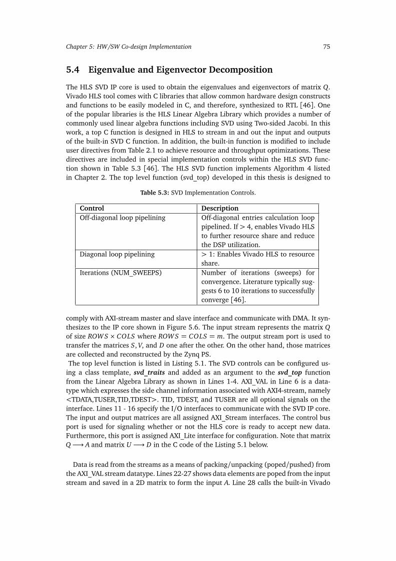
Chapter 5: HW/SW Co-design Implementation 75
5.4 Eigenvalue and Eigenvector Decomposition
The HLS SVD IP core is used to obtain the eigenvalues and eigenvectors of matrix Q.Vivado HLS tool comes with C libraries that allow common hardware design constructsand functions to be easily modeled in C, and therefore, synthesized to RTL [46]. Oneof the popular libraries is the HLS Linear Algebra Library which provides a number ofcommonly used linear algebra functions including SVD using Two-sided Jacobi. In thiswork, a top C function is designed in HLS to stream in and out the input and outputsof the built-in SVD C function. In addition, the built-in function is modified to includeuser directives from Table 2.1 to achieve resource and throughput optimizations. Thesedirectives are included in special implementation controls within the HLS SVD func-tion shown in Table 5.3 [46]. The HLS SVD function implements Algorithm 4 listedin Chapter 2. The top level function (svd_top) developed in this thesis is designed to
Table 5.3: SVD Implementation Controls.
Control DescriptionOff-diagonal loop pipelining Off-diagonal entries calculation loop
pipelined. If > 4, enables Vivado HLSto further resource share and reducethe DSP utilization.
Diagonal loop pipelining > 1: Enables Vivado HLS to resourceshare.
Iterations (NUM_SWEEPS) Number of iterations (sweeps) forconvergence. Literature typically sug-gests 6 to 10 iterations to successfullyconverge [46].
comply with AXI-stream master and slave interface and communicate with DMA. It syn-thesizes to the IP core shown in Figure 5.6. The input stream represents the matrix Qof size ROWS × COLS where ROWS = COLS = m. The output stream port is used totransfer the matrices S, V, and D one after the other. On the other hand, those matricesare collected and reconstructed by the Zynq PS.The top level function is listed in Listing 5.1. The SVD controls can be configured us-
ing a class template, svd_traits and added as an argument to the svd_top functionfrom the Linear Algebra Library as shown in Lines 1-4. AXI_VAL in Line 6 is a data-type which expresses the side channel information associated with AXI4-stream, namely<TDATA,TUSER,TID,TDEST>. TID, TDEST, and TUSER are all optional signals on theinterface. Lines 11 - 16 specify the I/O interfaces to communicate with the SVD IP core.The input and output matrices are all assigned AXI_Stream interfaces. The control busport is used for signaling whether or not the HLS core is ready to accept new data.Furthermore, this port is assigned AXI_Lite interface for configuration. Note that matrixQ −→ A and matrix U −→ D in the C code of the Listing 5.1 below.
Data is read from the streams as a means of packing/unpacking (poped/pushed) fromthe AXI_VAL stream datatype. Lines 22-27 shows data elements are poped from the inputstream and saved in a 2D matrix to form the input A. Line 28 calls the built-in Vivado

76 5.4 Eigenvalue and Eigenvector Decomposition
Figure 5.6: HLS SVD block design.
HLS SVD function with the user defined control configuration. The computed SUV datastored in memory (BRAM tiles when converted to RTL) is pushed to the output streamsequentially in Lines 30-47. Notice that a TLAST signal is concatenated with the last Velement in Line 45. This signal is set high when (k = ROWS ∗ COLS ∗ 3− 1), in otherwords, the last computed element is streamed.
Code listing 5.1: HLS SVD C code.
1 struct MY_CONFIG : hls::svd_traits<A_ROWS,A_COLS,MATRIX_IN_T,MATRIX_OUT_T>{2 static const int NUM_SWEEPS = 6;3 static const int DIAG_II = 4;4 static const int OFF_DIAG_II = 4;5 };6 typedef ap_axiu<32,1,1,1> AXI_VAL;7 // The top-level function to synthesize8 //9 void svd_top (AXI_VAL INPUT_STREAM[A_ROWS*A_COLS], AXI_VAL OUTPUT_STREAM[A_ROWS*A_COLS*3])
10 {11 #pragma HLS INTERFACE axis port=INPUT_STREAM12 #pragma HLS INTERFACE axis port=OUTPUT_STREAM13 // axi lite interface is used by the ARM processor to control the execution of this accelerator14 // this line also creates an interrupt port for this module which later will be used by15 // Zynq PS code to signal that data is ready.16 #pragma HLS INTERFACE s_axilite port=return bundle=CONTROL_BUS17 MATRIX_IN_T a_i[A_ROWS][A_COLS];18 MATRIX_OUT_T s_i[A_ROWS][A_COLS];19 MATRIX_OUT_T u_i[A_ROWS][A_ROWS];20 MATRIX_OUT_T v_i[A_COLS][A_COLS];21 // Copy input data to local memory22 a_row_loop : for (int r=0;r<A_ROWS;r++) {23 a_col_loop : for (int c=0;c<A_COLS;c++) {24 int k = r*A_ROWS + c;25 a_i[r][c] = pop_stream<float,1,1,1>(INPUT_STREAM[k]);26 }27 }28 hls::svd<A_ROWS, A_COLS, MATRIX_IN_T, MATRIX_OUT_T>(a_i, MY_CONFIG, s_i, u_i, v_i);29 // Copy local memory contents to outputs30 s_row_loop : for (int r=0;r<A_ROWS;r++) {31 s_col_loop : for (int c=0;c<A_COLS;c++) {32 int k = r*A_ROWS + c;33 OUTPUT_STREAM[k] = push_stream<float, 1, 1, 1>(s_i[r][c]);34 }
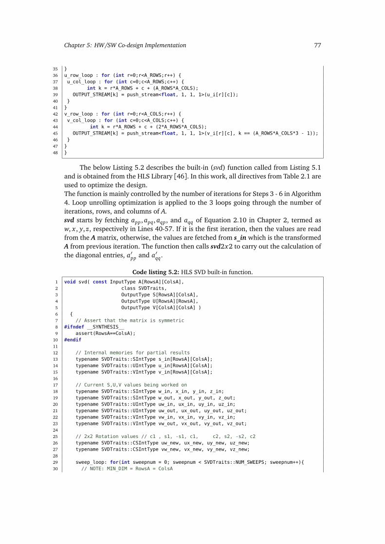
Chapter 5: HW/SW Co-design Implementation 77
35 }36 u_row_loop : for (int r=0;r<A_ROWS;r++) {37 u_col_loop : for (int c=0;c<A_ROWS;c++) {38 int k = r*A_ROWS + c + (A_ROWS*A_COLS);39 OUTPUT_STREAM[k] = push_stream<float, 1, 1, 1>(u_i[r][c]);40 }41 }42 v_row_loop : for (int r=0;r<A_COLS;r++) {43 v_col_loop : for (int c=0;c<A_COLS;c++) {44 int k = r*A_ROWS + c + (2*A_ROWS*A_COLS);45 OUTPUT_STREAM[k] = push_stream<float, 1, 1, 1>(v_i[r][c], k == (A_ROWS*A_COLS*3 - 1));46 }47 }48 }
The below Listing 5.2 describes the built-in (svd) function called from Listing 5.1and is obtained from the HLS Library [46]. In this work, all directives from Table 2.1 areused to optimize the design.The function is mainly controlled by the number of iterations for Steps 3 - 6 in Algorithm4. Loop unrolling optimization is applied to the 3 loops going through the number ofiterations, rows, and columns of A.svd starts by fetching app, apq, aqp, and aqq of Equation 2.10 in Chapter 2, termed asw, x , y, z, respectively in Lines 40-57. If it is the first iteration, then the values are readfrom the A matrix, otherwise, the values are fetched from s_in which is the transformedA from previous iteration. The function then calls svd2x2 to carry out the calculation ofthe diagonal entries, a′pp and a′qq.
Code listing 5.2: HLS SVD built-in function.
1 void svd( const InputType A[RowsA][ColsA],2 class SVDTraits,3 OutputType S[RowsA][ColsA],4 OutputType U[RowsA][RowsA],5 OutputType V[ColsA][ColsA] )6 {7 // Assert that the matrix is symmetric8 #ifndef __SYNTHESIS__9 assert(RowsA==ColsA);
10 #endif1112 // Internal memories for partial results13 typename SVDTraits::SIntType s_in[RowsA][ColsA];14 typename SVDTraits::UIntType u_in[RowsA][ColsA];15 typename SVDTraits::VIntType v_in[RowsA][ColsA];1617 // Current S,U,V values being worked on18 typename SVDTraits::SIntType w_in, x_in, y_in, z_in;19 typename SVDTraits::SIntType w_out, x_out, y_out, z_out;20 typename SVDTraits::UIntType uw_in, ux_in, uy_in, uz_in;21 typename SVDTraits::UIntType uw_out, ux_out, uy_out, uz_out;22 typename SVDTraits::VIntType vw_in, vx_in, vy_in, vz_in;23 typename SVDTraits::VIntType vw_out, vx_out, vy_out, vz_out;2425 // 2x2 Rotation values // c1 , s1, -s1, c1, c2, s2, -s2, c226 typename SVDTraits::CSIntType uw_new, ux_new, uy_new, uz_new;27 typename SVDTraits::CSIntType vw_new, vx_new, vy_new, vz_new;2829 sweep_loop: for(int sweepnum = 0; sweepnum < SVDTraits::NUM_SWEEPS; sweepnum++){30 // NOTE: MIN_DIM = RowsA = ColsA

78 5.4 Eigenvalue and Eigenvector Decomposition
31 #pragma HLS UNROLL FACTOR = SVDTraits::DIAG_UNROLL_FACTOR32 row_loop: for(int top_left = 0; top_left < SVDTraits::MIN_DIM; top_left++) {33 #pragma HLS UNROLL FACTOR = SVDTraits::DIAG_UNROLL_FACTOR34 col_loop: for(int bottom_right = top_left+1;35 bottom_right< SVDTraits::MIN_DIM; bottom_right++) {36 // loop unrolling and Pipelining37 #pragma HLS UNROLL FACTOR = SVDTraits::DIAG_UNROLL_FACTOR38 #pragma HLS PIPELINE II = SVDTraits::DIAG_II39 // Fetch w,x,y,z values40 if (sweepnum == 0 && top_left == 0) {41 if (bottom_right == 1) {42 w_in =A[top_left] [top_left];43 x_in =A[top_left] [bottom_right];44 y_in =A[bottom_right][top_left];45 } else {46 // Now revist values already updated in first diagonal pass47 w_in =s_in[top_left] [top_left];48 x_in =s_in[top_left] [bottom_right];49 y_in =s_in[bottom_right][top_left];50 }51 z_in =A[bottom_right][bottom_right];52 } else {53 w_in =s_in[top_left] [top_left];54 x_in =s_in[top_left] [bottom_right];55 y_in =s_in[bottom_right][top_left];56 z_in =s_in[bottom_right][bottom_right];57 }5859 // Diagonal60 svd2x2(w_in, x_in, y_in, z_in, uw_new, ux_new,61 uy_new, uz_new, vw_new, vx_new, vy_new, vz_new,62 w_out, x_out, y_out, z_out);
svd2x2 function is described in Listing 5.3. This function is inlined when being calledby svd in the previous code listing. Lines 22-33 compute half angles θ1 and θ2 by mak-ing use of arctan for Equation 2.13. Next, Lines 36-61 carry out matrix multiplicationswhich corresponds to Equations 2.15 and 2.16 by making use of an inlined function,vm2x1(a1, b1, a2, b2, c), which simply computes c = a1 ∗ b1+ a2 ∗ b2.
Code listing 5.3: svd2x2 function.
1 void svd2x2(2 AInType w_in, AInType x_in, AInType y_in, AInType z_in,3 CSType &uw_out, CSType &ux_out, CSType &uy_out, CSType &uz_out,4 CSType &vw_out, CSType &vx_out, CSType &vy_out, CSType &vz_out,5 AOutType &w_out, AOutType &x_out, AOutType &y_out, AOutType &z_out)6 {7 // svd2x2 is inlined in into any functions calling svd2x28 #pragma HLS inline9 const AOutType outZERO = 0;
10 CSType s1, c1, s2, c2;11 AInType u1, u2;12 std::complex<AInType> A, B;13 CSType cosA_full, sinA_full, cosA_half, sinA_half;14 CSType cosB_full, sinB_full, cosB_half, sinB_half;15 bool A_is_pos_real, A_is_imag;16 bool B_is_pos_real, B_is_imag;17 CSType uw_int, ux_int, uy_int, uz_int;18 CSType vw_int, vx_int, vy_int, vz_int;19 AOutType w_out1, w_out2, z_out1, z_out2,20 w_out_int, z_out_int;21 // Determine first half angle required to zero off-diagonal values
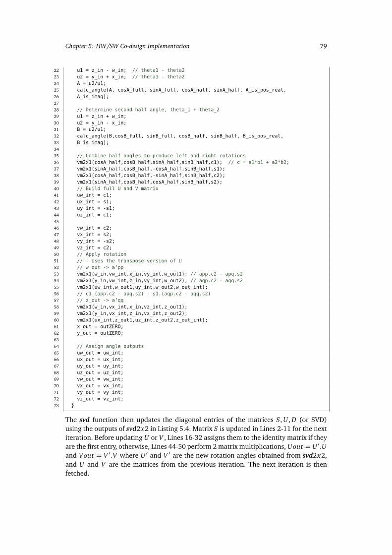
Chapter 5: HW/SW Co-design Implementation 79
22 u1 = z_in - w_in; // theta1 - theta223 u2 = y_in + x_in; // theta1 - theta224 A = u2/u1;25 calc_angle(A, cosA_full, sinA_full, cosA_half, sinA_half, A_is_pos_real,26 A_is_imag);2728 // Determine second half angle, theta_1 + theta_229 u1 = z_in + w_in;30 u2 = y_in - x_in;31 B = u2/u1;32 calc_angle(B,cosB_full, sinB_full, cosB_half, sinB_half, B_is_pos_real,33 B_is_imag);3435 // Combine half angles to produce left and right rotations36 vm2x1(cosA_half,cosB_half,sinA_half,sinB_half,c1); // c = a1*b1 + a2*b2;37 vm2x1(sinA_half,cosB_half,-cosA_half,sinB_half,s1);38 vm2x1(cosA_half,cosB_half,-sinA_half,sinB_half,c2);39 vm2x1(sinA_half,cosB_half,cosA_half,sinB_half,s2);40 // Build full U and V matrix41 uw_int = c1;42 ux_int = s1;43 uy_int = -s1;44 uz_int = c1;4546 vw_int = c2;47 vx_int = s2;48 vy_int = -s2;49 vz_int = c2;50 // Apply rotation51 // - Uses the transpose version of U52 // w_out -> a’pp53 vm2x1(w_in,vw_int,x_in,vy_int,w_out1); // app.c2 - apq.s254 vm2x1(y_in,vw_int,z_in,vy_int,w_out2); // aqp.c2 - aqq.s255 vm2x1(uw_int,w_out1,uy_int,w_out2,w_out_int);56 // c1.(app.c2 - apq.s2) - s1.(aqp.c2 - aqq.s2)57 // z_out -> a’qq58 vm2x1(w_in,vx_int,x_in,vz_int,z_out1);59 vm2x1(y_in,vx_int,z_in,vz_int,z_out2);60 vm2x1(ux_int,z_out1,uz_int,z_out2,z_out_int);61 x_out = outZERO;62 y_out = outZERO;6364 // Assign angle outputs65 uw_out = uw_int;66 ux_out = ux_int;67 uy_out = uy_int;68 uz_out = uz_int;69 vw_out = vw_int;70 vx_out = vx_int;71 vy_out = vy_int;72 vz_out = vz_int;73 }
The svd function then updates the diagonal entries of the matrices S, U , D (or SVD)using the outputs of svd2x2 in Listing 5.4. Matrix S is updated in Lines 2-11 for the nextiteration. Before updating U or V , Lines 16-32 assigns them to the identity matrix if theyare the first entry, otherwise, Lines 44-50 perform 2 matrix multiplications, Uout = U ′.Uand Vout = V ′.V where U ′ and V ′ are the new rotation angles obtained from svd2x2,and U and V are the matrices from the previous iteration. The next iteration is thenfetched.
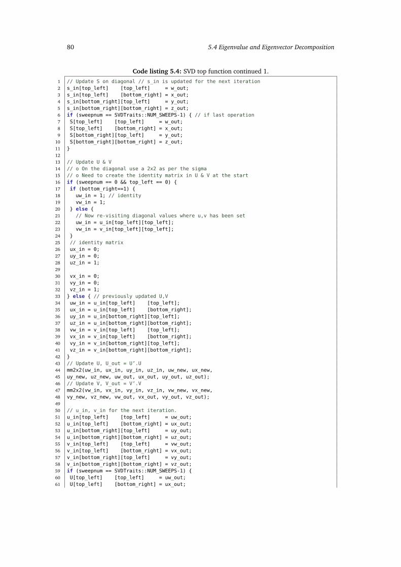
80 5.4 Eigenvalue and Eigenvector Decomposition
Code listing 5.4: SVD top function continued 1.
1 // Update S on diagonal // s_in is updated for the next iteration2 s_in[top_left] [top_left] = w_out;3 s_in[top_left] [bottom_right] = x_out;4 s_in[bottom_right][top_left] = y_out;5 s_in[bottom_right][bottom_right] = z_out;6 if (sweepnum == SVDTraits::NUM_SWEEPS-1) { // if last operation7 S[top_left] [top_left] = w_out;8 S[top_left] [bottom_right] = x_out;9 S[bottom_right][top_left] = y_out;
10 S[bottom_right][bottom_right] = z_out;11 }1213 // Update U & V14 // o On the diagonal use a 2x2 as per the sigma15 // o Need to create the identity matrix in U & V at the start16 if (sweepnum == 0 && top_left == 0) {17 if (bottom_right==1) {18 uw_in = 1; // identity19 vw_in = 1;20 } else {21 // Now re-visiting diagonal values where u,v has been set22 uw_in = u_in[top_left][top_left];23 vw_in = v_in[top_left][top_left];24 }25 // identity matrix26 ux_in = 0;27 uy_in = 0;28 uz_in = 1;2930 vx_in = 0;31 vy_in = 0;32 vz_in = 1;33 } else { // previously updated U,V34 uw_in = u_in[top_left] [top_left];35 ux_in = u_in[top_left] [bottom_right];36 uy_in = u_in[bottom_right][top_left];37 uz_in = u_in[bottom_right][bottom_right];38 vw_in = v_in[top_left] [top_left];39 vx_in = v_in[top_left] [bottom_right];40 vy_in = v_in[bottom_right][top_left];41 vz_in = v_in[bottom_right][bottom_right];42 }43 // Update U, U_out = U’.U44 mm2x2(uw_in, ux_in, uy_in, uz_in, uw_new, ux_new,45 uy_new, uz_new, uw_out, ux_out, uy_out, uz_out);46 // Update V, V_out = V’.V47 mm2x2(vw_in, vx_in, vy_in, vz_in, vw_new, vx_new,48 vy_new, vz_new, vw_out, vx_out, vy_out, vz_out);4950 // u_in, v_in for the next iteration.51 u_in[top_left] [top_left] = uw_out;52 u_in[top_left] [bottom_right] = ux_out;53 u_in[bottom_right][top_left] = uy_out;54 u_in[bottom_right][bottom_right] = uz_out;55 v_in[top_left] [top_left] = vw_out;56 v_in[top_left] [bottom_right] = vx_out;57 v_in[bottom_right][top_left] = vy_out;58 v_in[bottom_right][bottom_right] = vz_out;59 if (sweepnum == SVDTraits::NUM_SWEEPS-1) {60 U[top_left] [top_left] = uw_out;61 U[top_left] [bottom_right] = ux_out;
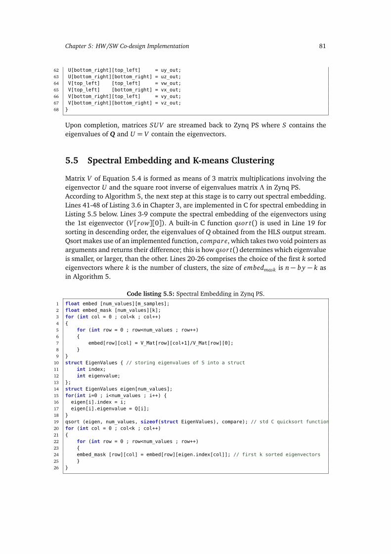
Chapter 5: HW/SW Co-design Implementation 81
62 U[bottom_right][top_left] = uy_out;63 U[bottom_right][bottom_right] = uz_out;64 V[top_left] [top_left] = vw_out;65 V[top_left] [bottom_right] = vx_out;66 V[bottom_right][top_left] = vy_out;67 V[bottom_right][bottom_right] = vz_out;68 }
Upon completion, matrices SUV are streamed back to Zynq PS where S contains theeigenvalues of Q and U = V contain the eigenvectors.
5.5 Spectral Embedding and K-means Clustering
Matrix V of Equation 5.4 is formed as means of 3 matrix multiplications involving theeigenvector U and the square root inverse of eigenvalues matrix Λ in Zynq PS.According to Algorithm 5, the next step at this stage is to carry out spectral embedding.Lines 41-48 of Listing 3.6 in Chapter 3, are implemented in C for spectral embedding inListing 5.5 below. Lines 3-9 compute the spectral embedding of the eigenvectors usingthe 1st eigenvector (V [row][0]). A built-in C function qsor t() is used in Line 19 forsorting in descending order, the eigenvalues of Q obtained from the HLS output stream.Qsort makes use of an implemented function, compare, which takes two void pointers asarguments and returns their difference; this is how qsor t() determines which eigenvalueis smaller, or larger, than the other. Lines 20-26 comprises the choice of the first k sortedeigenvectors where k is the number of clusters, the size of embedmask is n− b y − k asin Algorithm 5.
Code listing 5.5: Spectral Embedding in Zynq PS.
1 float embed [num_values][m_samples];2 float embed_mask [num_values][k];3 for (int col = 0 ; col<k ; col++)4 {5 for (int row = 0 ; row<num_values ; row++)6 {7 embed[row][col] = V_Mat[row][col+1]/V_Mat[row][0];8 }9 }
10 struct EigenValues { // storing eigenvalues of S into a struct11 int index;12 int eigenvalue;13 };14 struct EigenValues eigen[num_values];15 for(int i=0 ; i<num_values ; i++) {16 eigen[i].index = i;17 eigen[i].eigenvalue = Q[i];18 }19 qsort (eigen, num_values, sizeof(struct EigenValues), compare); // std C quicksort function20 for (int col = 0 ; col<k ; col++)21 {22 for (int row = 0 ; row<num_values ; row++)23 {24 embed_mask [row][col] = embed[row][eigen.index[col]]; // first k sorted eigenvectors25 }26 }
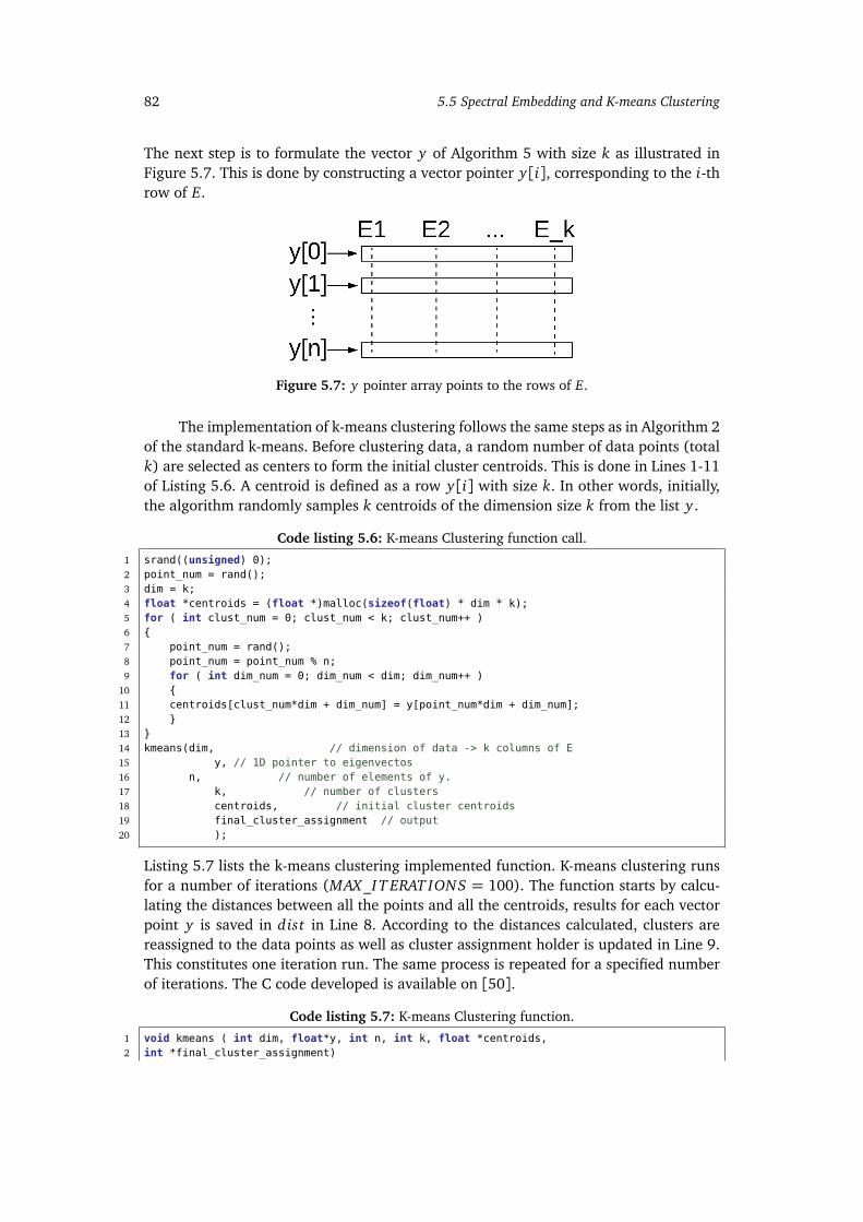
82 5.5 Spectral Embedding and K-means Clustering
The next step is to formulate the vector y of Algorithm 5 with size k as illustrated inFigure 5.7. This is done by constructing a vector pointer y[i], corresponding to the i-throw of E.
Figure 5.7: y pointer array points to the rows of E.
The implementation of k-means clustering follows the same steps as in Algorithm 2of the standard k-means. Before clustering data, a random number of data points (totalk) are selected as centers to form the initial cluster centroids. This is done in Lines 1-11of Listing 5.6. A centroid is defined as a row y[i] with size k. In other words, initially,the algorithm randomly samples k centroids of the dimension size k from the list y .
Code listing 5.6: K-means Clustering function call.
1 srand((unsigned) 0);2 point_num = rand();3 dim = k;4 float *centroids = (float *)malloc(sizeof(float) * dim * k);5 for ( int clust_num = 0; clust_num < k; clust_num++ )6 {7 point_num = rand();8 point_num = point_num % n;9 for ( int dim_num = 0; dim_num < dim; dim_num++ )
10 {11 centroids[clust_num*dim + dim_num] = y[point_num*dim + dim_num];12 }13 }14 kmeans(dim, // dimension of data -> k columns of E15 y, // 1D pointer to eigenvectos16 n, // number of elements of y.17 k, // number of clusters18 centroids, // initial cluster centroids19 final_cluster_assignment // output20 );
Listing 5.7 lists the k-means clustering implemented function. K-means clustering runsfor a number of iterations (MAX_I T ERAT IONS = 100). The function starts by calcu-lating the distances between all the points and all the centroids, results for each vectorpoint y is saved in dist in Line 8. According to the distances calculated, clusters arereassigned to the data points as well as cluster assignment holder is updated in Line 9.This constitutes one iteration run. The same process is repeated for a specified numberof iterations. The C code developed is available on [50].
Code listing 5.7: K-means Clustering function.
1 void kmeans ( int dim, float*y, int n, int k, float *centroids,2 int *final_cluster_assignment)
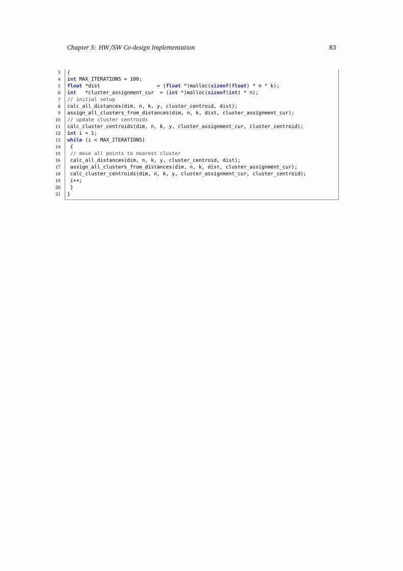
Chapter 5: HW/SW Co-design Implementation 83
3 {4 int MAX_ITERATIONS = 100;5 float *dist = (float *)malloc(sizeof(float) * n * k);6 int *cluster_assignment_cur = (int *)malloc(sizeof(int) * n);7 // initial setup8 calc_all_distances(dim, n, k, y, cluster_centroid, dist);9 assign_all_clusters_from_distances(dim, n, k, dist, cluster_assignment_cur);
10 // update cluster centroids11 calc_cluster_centroids(dim, n, k, y, cluster_assignment_cur, cluster_centroid);12 int i = 1;13 while (i < MAX_ITERATIONS)14 {15 // move all points to nearest cluster16 calc_all_distances(dim, n, k, y, cluster_centroid, dist);17 assign_all_clusters_from_distances(dim, n, k, dist, cluster_assignment_cur);18 calc_cluster_centroids(dim, n, k, y, cluster_assignment_cur, cluster_centroid);19 i++;20 }21 }

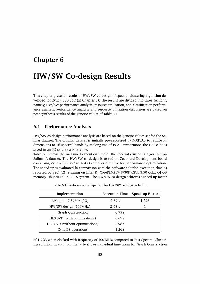
Chapter 6
HW/SW Co-design Results
This chapter presents results of HW/SW co-design of spectral clustering algorithm de-veloped for Zynq-7000 SoC (in Chapter 5). The results are divided into three sections,namely, HW/SW performance analysis, resource utilization, and classification perform-ance analysis. Performance analysis and resource utilization discussion are based onpost-synthesis results of the generic values of Table 5.1
6.1 Performance Analysis
HW/SW co-design performance analysis are based on the generic values set for the Sa-linas dataset. The original dataset is initially pre-processed by MATLAB to reduce itsdimensions to 16 spectral bands by making use of PCA. Furthermore, the HSI cube issaved in an SD card as a binary file.Table 6.1 shows the measured execution time of the spectral clustering algorithm onSalinas-A dataset. The HW/SW co-design is tested on Zedboard Development boardcontaining Zynq-7000 SoC with -O3 compiler directive for performance optimization.The speed-up is evaluated in comparison with the software solution execution time asreported by FSC [12] running on Intel(R) Core(TM) i7-5930K CPU, 3.50 GHz, 64 GBmemory, Ubuntu 14.04.5 LTS system. The HW/SW co-design achieves a speed-up factor
Table 6.1: Performance comparison for HW/SW codesign solution.
Implementation Execution Time Speed-up Factor
FSC Intel i7-5930K [12] 4.62 s 1.723
HW/SW design (100MHz) 2.68 s 1
Graph Construction 0.75 s
HLS SVD (with optimizations) 0.67 s
HLS SVD (without optimizations) 2.98 s
Zynq PS operations 1.26 s
of 1.723 when clocked with frequency of 100 MHz compared to Fast Spectral Cluster-ing solution. In addition, the table shows individual time taken for Graph Construction
85

86 6.2 Resource Utilization
of A and B module and the HLS SVD module. Hardware timings are measured usingAXI_TIMER and maximum clock latency/clock cycles. It can be observed that the HLSSVD core is the most expensive module in time complexity. This is because of the largematrix data that is decomposed into 3 other matrices of the same size. Furthermore,time has been measured with and without the user directive, resource and throughput,optimizations of Tables 2.1 and 5.3. The optimization owed to a speed-up factor of 4.45for the HLS SVD core performance.Zynq PS operations time includes the total time taken for HSI read from SD, two datatransfers, Q and V matrix formations, spectral embedding, and k-means clustering. Soft-ware time is measured using C XTime library.
The highest achievable operating frequencies for modules synthesized on XC7Z020-CLG484-1 SoC are shown in Table 6.2. Each hardware module in the design have beenindividually analyzed to determine the maximum operating frequencies by making useof the timing reports.
Table 6.2: Maximum frequency for HW/SW codesign solution modules.
Module Minimum Time Period Maximum Frequency
PS-PL System 9.955 ns 100.45 MHz
Graph Construction 6.270 ns 159.48 MHz
HLS SVD 6.343 ns 157.63 MHz
Master Output 2.362 ns 423.45 MHz
BRAM Module 3.363 ns 297.35 MHz
6.2 Resource Utilization
Post-synthesis resource utilization for HW/SW co-design using the generic parametersis shown in Table 6.3. The table shows the total resources used and their percentage ofthe total resources available on xc7z020clg484-1 SoC. HSI data input saved in BRAMmodule is synthesized to use 64 BRAM tiles which accounts for approximately for 45.7%of the available BRAM on the SoC device. As for HLS SVD core, the used BRAM tilesaccounts for 16.4% of the total BRAM tiles available.
The high use of BRAM tiles (77.14% with 16 spectral bands) can be a limitationfor this HW/SW co-design solution. Figure 6.1 shows the BRAM module resource utiliza-tion of BRAM tiles, slice LUTs, and slice registers as a function of the number of spectralbands varrying from 16 to 32 in steps of 4. The limitation can be observed at 28 spec-tral bands where the total number of synthesized BRAM tiles (BRAM module + PL)goes beyond the available resources (140 BRAM tiles). This is because as the number ofspectral bands increases, the size of the HSI cube increases as well. Consequently, theBRAM_ADDR_WIDTH parameter increases and more BRAM rows are required by thedesign. However, the design meets the requirements outlined in section 1.2 of operatingon at least 20 spectral bands. In addition, as expected, slice LUTs and registers slightlyincrease with the number of spectral bands.
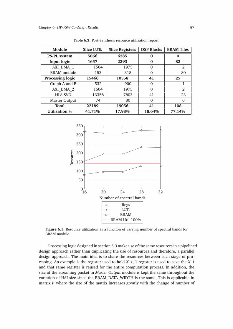
Chapter 6: HW/SW Co-design Results 87
Table 6.3: Post-Synthesis resource utilization report.
Module Slice LUTs Slice Registers DSP Blocks BRAM Tiles
PS-PL system 5066 6285 0 0Input logic 1657 2293 0 82
AXI_DMA_1 1504 1975 0 2BRAM module 153 318 0 80
Processing logic 15466 10558 41 25Graph A and B 532 900 0 1AXI_DMA_2 1504 1975 0 2
HLS SVD 13356 7603 41 23Master Output 74 80 0 0
Total 22189 19056 41 108Utilization % 41.71% 17.98% 18.64% 77.14%
16 20 24 28 320
50
100
150
200
250
300
350
Number of spectral bands
Res
ourc
e
RegsLUTs
BRAMBRAM Util 100%
Figure 6.1: Resource utilization as a function of varying number of spectral bands forBRAM module.
Processing logic designed in section 5.3 make use of the same resources in a pipelineddesign approach rather than duplicating the use of resources and therefore, a paralleldesign approach. The main idea is to share the resources between each stage of pro-cessing. An example is the register used to hold X_i, 1 register is used to save the X_iand that same register is reused for the entire computation process. In addition, thesize of the streaming packet in Master Output module is kept the same throughout thevariation of HSI size since the BRAM_DATA_WIDTH is the same. This is applicable inmatrix B where the size of the matrix increases greatly with the change of number of
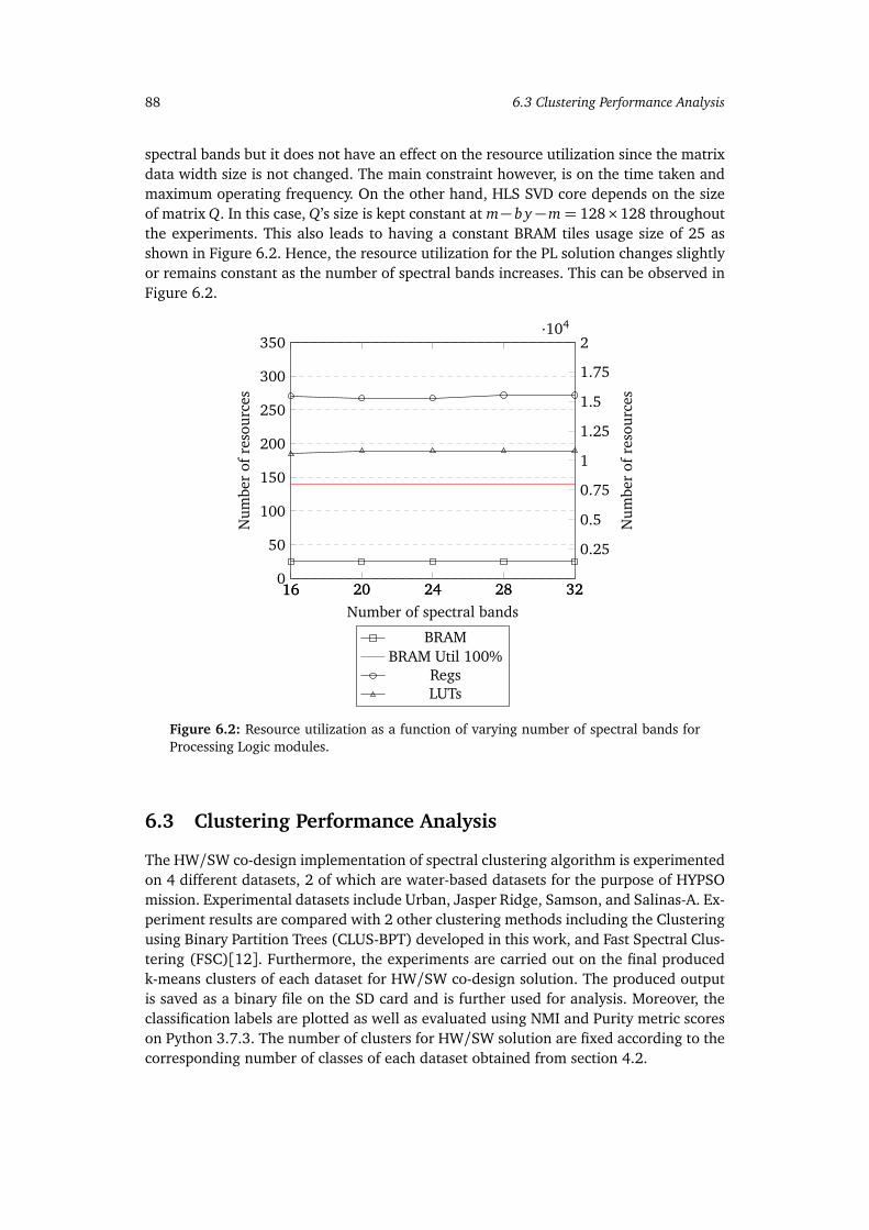
88 6.3 Clustering Performance Analysis
spectral bands but it does not have an effect on the resource utilization since the matrixdata width size is not changed. The main constraint however, is on the time taken andmaximum operating frequency. On the other hand, HLS SVD core depends on the sizeof matrix Q. In this case, Q’s size is kept constant at m− b y−m= 128×128 throughoutthe experiments. This also leads to having a constant BRAM tiles usage size of 25 asshown in Figure 6.2. Hence, the resource utilization for the PL solution changes slightlyor remains constant as the number of spectral bands increases. This can be observed inFigure 6.2.
16 20 24 28 32
0.25
0.5
0.75
1
1.25
1.5
1.75
2·104
Number of spectral bandsN
umbe
rof
reso
urce
sBRAM
BRAM Util 100%RegsLUTs
16 20 24 28 320
50
100
150
200
250
300
350
Num
ber
ofre
sour
ces
Figure 6.2: Resource utilization as a function of varying number of spectral bands forProcessing Logic modules.
6.3 Clustering Performance Analysis
The HW/SW co-design implementation of spectral clustering algorithm is experimentedon 4 different datasets, 2 of which are water-based datasets for the purpose of HYPSOmission. Experimental datasets include Urban, Jasper Ridge, Samson, and Salinas-A. Ex-periment results are compared with 2 other clustering methods including the Clusteringusing Binary Partition Trees (CLUS-BPT) developed in this work, and Fast Spectral Clus-tering (FSC)[12]. Furthermore, the experiments are carried out on the final producedk-means clusters of each dataset for HW/SW co-design solution. The produced outputis saved as a binary file on the SD card and is further used for analysis. Moreover, theclassification labels are plotted as well as evaluated using NMI and Purity metric scoreson Python 3.7.3. The number of clusters for HW/SW solution are fixed according to thecorresponding number of classes of each dataset obtained from section 4.2.
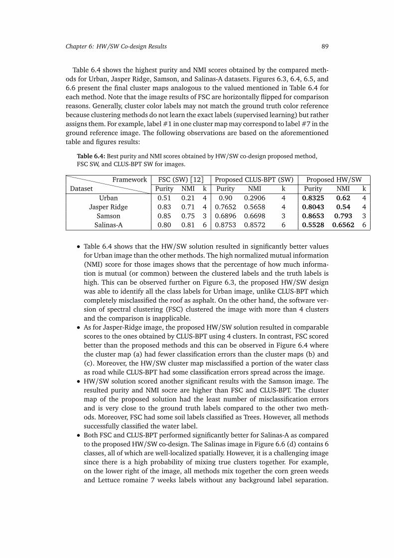
Chapter 6: HW/SW Co-design Results 89
Table 6.4 shows the highest purity and NMI scores obtained by the compared meth-ods for Urban, Jasper Ridge, Samson, and Salinas-A datasets. Figures 6.3, 6.4, 6.5, and6.6 present the final cluster maps analogous to the valued mentioned in Table 6.4 foreach method. Note that the image results of FSC are horizontally flipped for comparisonreasons. Generally, cluster color labels may not match the ground truth color referencebecause clustering methods do not learn the exact labels (supervised learning) but ratherassigns them. For example, label #1 in one cluster map may correspond to label #7 in theground reference image. The following observations are based on the aforementionedtable and figures results:
Table 6.4: Best purity and NMI scores obtained by HW/SW co-design proposed method,FSC SW, and CLUS-BPT SW for images.
DatasetFramework FSC (SW) [12] Proposed CLUS-BPT (SW) Proposed HW/SW
Purity NMI k Purity NMI k Purity NMI kUrban 0.51 0.21 4 0.90 0.2906 4 0.8325 0.62 4
Jasper Ridge 0.83 0.71 4 0.7652 0.5658 4 0.8043 0.54 4Samson 0.85 0.75 3 0.6896 0.6698 3 0.8653 0.793 3
Salinas-A 0.80 0.81 6 0.8753 0.8572 6 0.5528 0.6562 6
• Table 6.4 shows that the HW/SW solution resulted in significantly better valuesfor Urban image than the other methods. The high normalized mutual information(NMI) score for those images shows that the percentage of how much informa-tion is mutual (or common) between the clustered labels and the truth labels ishigh. This can be observed further on Figure 6.3, the proposed HW/SW designwas able to identify all the class labels for Urban image, unlike CLUS-BPT whichcompletely misclassified the roof as asphalt. On the other hand, the software ver-sion of spectral clustering (FSC) clustered the image with more than 4 clustersand the comparison is inapplicable.
• As for Jasper-Ridge image, the proposed HW/SW solution resulted in comparablescores to the ones obtained by CLUS-BPT using 4 clusters. In contrast, FSC scoredbetter than the proposed methods and this can be observed in Figure 6.4 wherethe cluster map (a) had fewer classification errors than the cluster maps (b) and(c). Moreover, the HW/SW cluster map misclassified a portion of the water classas road while CLUS-BPT had some classification errors spread across the image.
• HW/SW solution scored another significant results with the Samson image. Theresulted purity and NMI socre are higher than FSC and CLUS-BPT. The clustermap of the proposed solution had the least number of misclassification errorsand is very close to the ground truth labels compared to the other two meth-ods. Moreover, FSC had some soil labels classified as Trees. However, all methodssuccessfully classified the water label.
• Both FSC and CLUS-BPT performed significantly better for Salinas-A as comparedto the proposed HW/SW co-design. The Salinas image in Figure 6.6 (d) contains 6classes, all of which are well-localized spatially. However, it is a challenging imagesince there is a high probability of mixing true clusters together. For example,on the lower right of the image, all methods mix together the corn green weedsand Lettuce romaine 7 weeks labels without any background label separation.

90 6.3 Clustering Performance Analysis
However, FSC and CLUS-BPT managed to separate distinct labels for the rest ofthe image while the proposed HW/SW solution struggled in partially identifyingthe lettuce romaine 5 weeks and mistakened it with lettuce romaine 6 weeks.
(a) (b) (c) (d)
(e)
Figure 6.3: Cluster maps obtained from (a) FSC [12], (b) proposed CLUS-BPT, (c) pro-posed HW/SW, (d) ground reference image, and (e) ground reference color codes ofclasses for Urban image.
(a) (b) (c) (d)
(e)
Figure 6.4: Cluster maps obtained from (a) FSC [12], (b) proposed CLUS-BPT, (c) pro-posed HW/SW, (d) ground reference image, and (e) ground reference color codes ofclasses for Jasper Ridge image.
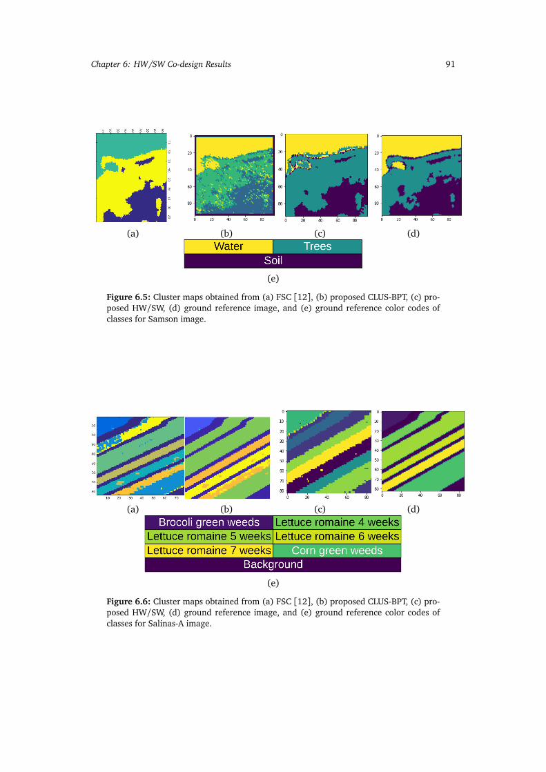
Chapter 6: HW/SW Co-design Results 91
(a) (b) (c) (d)
(e)
Figure 6.5: Cluster maps obtained from (a) FSC [12], (b) proposed CLUS-BPT, (c) pro-posed HW/SW, (d) ground reference image, and (e) ground reference color codes ofclasses for Samson image.
(a) (b) (c) (d)
(e)
Figure 6.6: Cluster maps obtained from (a) FSC [12], (b) proposed CLUS-BPT, (c) pro-posed HW/SW, (d) ground reference image, and (e) ground reference color codes ofclasses for Salinas-A image.


Chapter 7
Conclusion
In this thesis, unsupervised clustering classification for hypersepctral imagery has beenpresented as a very promising area of research [4]. Two solutions were proposed, namely,a software framework of filtering k-means clustering based on binary partition trees seg-mentation, and a hardware/software co-design implementation of spectral clusteringusing Nyström Extension. The two algorithm implementations have been profiled onsoftware for performance including classification evaluation scores and computationaltime. Furthermore, both software designs were tested on 8 widely used hyperspectralimage datasets. The results of the experimented designs serve as a solid ground for theHW/SW solution implementation. The software versions of the two algorithms are de-veloped using MATLAB R2019a and Python 3.7.3, respectively. On the other hand, theHW/SW co-design made use of a number of different development tools including XilinxVivado Design Suite, Vivado HLS, Xilinx SDK, and MathWorks HDL Coder™.
Unsupervised clustering classification has been preferred in this work to other classi-fication methods since clustering succeeds in: 1) identifying the number of class labelsin an image regardless of how many/what classes is the data divided into and 2) be-ing based on linear algebra computations which are very feasible to be implemented onFPGAs.
For CLUS-BPT, the framework made use of segmentation based on binary partitiontrees. This tree-based structure has been preferred in a hyperspectral image contextsince BPT proved to be accurately presenting: 1) the decomposition of the image interms of regions representing significant parts of the hyperspectral image and 2) the in-clusion relations of the regions in the scene [9]. Furthermore, given its fixed structure,BPT allows implementing efficient and advanced application-dependent techniques onit including k-means clustering algorithm. The k-means clustering is based on a filteringalgorithm that applies k-means clustering on tree-based data structures. Principal com-ponent analysis is integrated in the design to get the maximum data variance directionwhich is embedded with the final segmentation map in a new clustering framework.
Spectral clustering using Nyström Extension software algorithm was adapted from[37] and its implementation on hyperspectral images was inspired from [12]. Moreover,
93
the affinity matrix of the entire HSI cube is efficiently approximated using Nyström Ex-tension and is applicable to large-scale hyperspectral image datasets. The HW/SW solu-tion made use of the algorithm presented in [37]where eigenvalue decomposition of theLaplacian matrix represented a major challenge for this method. Instead, the eigenvaluedecomposition is found for a smaller size matrix using singular valued decomposition(SVD). A more optimized high-level synthesis of singular value decomposition is imple-mented using Vivado HLS. HW/SW cluster label results presented challenging evalu-ation scores as compared to other clustering methods. Moreover, the HW/SW solutionmaintains or even improves the clustering quality of the software version in 3 out of 4experimented HSI datasets.
7.1 Future Work
Both designs of the proposed methods are divided into a number of different componentsand stages that can be modified or replaced with other applicable parts. This createsmore room for future development and experiments, some of which are summarizedbelow:
• For CLUS-BPT, dimensionality reduction can be done using methods other thanPCA such as Linear Discriminant Analysis (LDA) and Non-negative matrix factor-ization (NMF). Both methods are used in pattern recognition context for featureextraction. In addition, NMF is able to preserve more information than PCA asdemonstrated by [51]. A further research can be done on the effect of number ofPCA components of a reduced HSI cube on the clustering performance.
• The HW/SW co-design takes advantage of the inherent parallelism in the designimplementation by using the pipeline approach. Hence, less hardware resourcesare used but this trades-off the execution time. Accordingly, HW/SW design can beintensively parallelized at many points including graph construction of matrices Aand B. In addition, further testing is necessary on different HSI datasets to definepossible improvements and limitations.
• Full FPGA implementation is possible for the software computations of the HW/SWsolution. This is because there exists in literature a number of FPGA implementa-tions for matrix multiplications and k-means clustering. However, the design couldbe limited by the hardware resources available to use on-board.
94
Bibliography
[1] S. Watson, B. Whitton, S. Higgins, H. Paerl, B. Brooks and J. Wehr, ‘Harmful algalblooms’, in. Jun. 2015, pp. 873–920, ISBN: 9780123858764. DOI: 10.1016/B978-0-12-385876-4.00020-7.
[2] The algae bloom in northern norway. [Online]. Available: https://www.kontali.no/references/fhf_901574.
[3] Mariusz E. Grøtte, Roger Birkeland, Joao F. Fortuna, Julian Veisdal, Milica Or-landic, Evelyn Honore-Livermore, Gara Quintana-Diaz, Harald Martens, J. TommyGravdahl„ Fred Sigernes, Jan Otto Reberg, Geir Johnsen, Kanna Rajan, and TorA. Johansen, ‘Hyperspectral imaging small satellite in multi-agent marine obser-vation system’, Unpublished-Internal document, 2018.
[4] D. Chutia, D. K. Bhattacharyya, K. K. Sarma, R. Kalita and S. Sudhakar, ‘Hyper-spectral remote sensing classifications: A perspective survey’, Transactions in GIS,Aug. 2015. DOI: 10.1111/tgis.12164.
[5] A. Signoroni, M. Savardi, A. Baronio and S. Benini, ‘Deep learning meets hyper-spectral image analysis: A multidisciplinary review’, Journal of Imaging, vol. 5,p. 52, May 2019. DOI: 10.3390/jimaging5050052.
[6] M. Ismail, ‘Unsupervised clustering for hyperspectral image classification’, 2019.
[7] J. Lei, L. Wu, Y. Li, W. Xie, C.-I. Chang, J. Zhang and B. Huang, ‘A novel fpga-basedarchitecture for fast automatic target detection in hyperspectral images’, RemoteSensing, vol. 11, p. 146, Jan. 2019. DOI: 10.3390/rs11020146.
[8] D. Lavenier, ‘Fpga implementation of the k-means clustering algorithm for hyper-spectral images’, Sep. 2000.
[9] S. Valero, P. Salembier and J. Chanussot, ‘Hyperspectral image representation andprocessing with binary partition trees’, IEEE transactions on image processing : apublication of the IEEE Signal Processing Society, vol. 22, Dec. 2012. DOI: 10.1109/TIP.2012.2231687.
[10] Cs231n: Convolutional neural networks for visual recognition, class notes for NeuralNetworks, Stanford, CA: Stanford Vision and Learning Lab, 2020. [Online]. Avail-able: https://cs231n.github.io/neural-networks-1/.
[11] S. Roy, G. Krishna, S. R. Dubey and B. Chaudhuri, ‘Hybridsn: Exploring 3d-2dcnn feature hierarchy for hyperspectral image classification’, Feb. 2019.
95
[12] Y. Zhao, Y. Yuan and Q. Wang, ‘Fast spectral clustering for unsupervised hyper-spectral image classification’, Remote Sensing, vol. 11, p. 399, Feb. 2019. DOI:10.3390/rs11040399.
[13] S. Ranjan, D. Nayak, S. Kumar, R. Dash and B. Majhi, ‘Hyperspectral image clas-sification: A k-means clustering based approach’, pp. 1–7, Jan. 2017. DOI: 10.1109/ICACCS.2017.8014707.
[14] A. Mehta and O. Dikshit, ‘Segmentation-based clustering of hyperspectral imagesusing local band selection’, Journal of Applied Remote Sensing, vol. 11, p. 015 028,Mar. 2017. DOI: 10.1117/1.JRS.11.015028.
[15] Y. Tarabalka, J. Benediktsson and J. Chanussot, ‘Spectral–spatial classification ofhyperspectral imagery based on partitional clustering techniques’, Geoscience andRemote Sensing, IEEE Transactions on, vol. 47, pp. 2973–2987, Sep. 2009. DOI:10.1109/TGRS.2009.2016214.
[16] V. Dey, Y. Zhang and M. Zhong, ‘A review on image segmentation techniques withremote sensing perspective’, ISPRS TC VII Symposium - 100 Years ISPRS, vol. 38,Jan. 2010.
[17] A. Mehta and O. Dikshit, ‘Projected clustering of hyperspectral imagery usingregion merging’, Remote Sensing Letters, vol. 7, pp. 721–730, Aug. 2016. DOI:10.1080/2150704X.2016.1182661.
[18] A. Mehta and O. Dikshit, ‘Segmentation-based projected clustering of hyperspec-tral images using mutual nearest neighbour’, IEEE Journal of Selected Topics inApplied Earth Observations and Remote Sensing, vol. PP, pp. 1–8, Nov. 2017. DOI:10.1109/JSTARS.2017.2768079.
[19] A. Mehta, A. Ashapure and O. Dikshit, ‘Segmentation based classification of hy-perspectral imagery using projected and correlation clustering techniques’, Geo-carto International, vol. 31, pp. 1–28, Oct. 2015. DOI: 10.1080/10106049.2015.1110207.
[20] C. Aggarwal, C. Procopiuc, J. Wolf, P. Yu and J. Park, ‘Fast algorithms for projectedclustering’, vol. 28, Jun. 1999, pp. 61–72. DOI: 10.1145/304181.304188.
[21] F. Winterstein, S. Bayliss and G. A. Constantinides, ‘Fpga-based k-means cluster-ing using tree-based data structures’, 23rd International Conference on Field pro-grammable Logic and Applications, 2013. [Online]. Available: https://ieeexplore.ieee.org/document/6645501/citations#citations.
[22] H. Futchs, Z. Kedem and B. Naylor, ‘On visible surface generation by a priori treestructures’, vol. 14, Dec. 1988, pp. 39–48. DOI: 10.1145/800250.807481.
[23] Y. Tarabalka, J. Chanussot and J. Benediktsson, ‘Segmentation and classificationof hyperspectral images using watershed transformation’, Pattern Recognition,vol. 43, pp. 2367–2379, Jul. 2010. DOI: 10.1016/j.patcog.2010.01.016.
[24] S. Beucher and F. Meyer, ‘The morphological approach to segmentation: The wa-tershed transformation’, in. Jan. 1993, vol. Vol. 34, pp. 433–481, ISBN: 9781315214610.DOI: 10.1201/9781482277234-12.
96
[25] G. Noyel, J. Angulo and D. Jeulin, ‘Morphological segmentation of hyperspectralimages’, Image Analysis and Stereology, Nov. 2007. DOI: 10.5566/ias.v26.p101-109.
[26] M. Veganzones, G. Tochon, M. Dalla Mura, A. Plaza and J. Chanussot, ‘Hyper-spectral image segmentation using a new spectral unmixing-based binary parti-tion tree representation’, IEEE transactions on image processing : a publication ofthe IEEE Signal Processing Society, vol. 23, Jun. 2014. DOI: 10.1109/TIP.2014.2329767.
[27] S. Valero, P. Salembier and J. Chanussot, ‘Comparison of merging orders and prun-ing strategies for binary partition tree in hyperspectral data’, Oct. 2010, pp. 2565–2568. DOI: 10.1109/ICIP.2010.5652595.
[28] S. Valero, P. Salembier, J. Chanussot and C. Cuadras, ‘Improved binary partitiontree construction for hyperspectral images: Application to object detection’, Aug.2011, pp. 2515–2518. DOI: 10.1109/IGARSS.2011.6049723.
[29] T. Kanungo, D. Mount, N. Netanyahu, C. Piatko, R. Silverman and A. Wu, ‘Anefficient k-means clustering algorithm analysis and implementation’, IEEE Trans-actions on Pattern Analysis and Machine Intelligence, vol. 24, pp. 881–892, Jul.2002. DOI: 10.1109/TPAMI.2002.1017616.
[30] T. Kanungo, D. Mount, N. Netanyahu, C. Piatko, R. Silverman and A. Wu, ‘Anefficient k-means clustering algorithm analysis and implementation’, IEEE Trans-actions on Pattern Analysis and Machine Intelligence, vol. 24, pp. 881–892, Jul.2002. DOI: 10.1109/TPAMI.2002.1017616.
[31] U. Luxburg, ‘A tutorial on spectral clustering’, Statistics and Computing, vol. 17,pp. 395–416, Jan. 2004. DOI: 10.1007/s11222-007-9033-z.
[32] J. Shi and J. Malik, ‘Normalized cuts and image segmentation’, IEEE Transactionson Pattern Analysis and Machine Intelligence, vol. 22, May 2002. DOI: 10.1109/34.868688.
[33] R. Bhatia, Positive Definite Matrices. Princeton University Press, 2007.
[34] N. J. Salkind, Encyclopedia of measurement and statistics. Sage, 2007.
[35] G. Strang, Introduction to Linear Algebra, Fourth. Wellesley, MA: Wellesley-CambridgePress, 2009, ISBN: 9780980232714.
[36] M. Berry, D. Mezher, B. Philippe and A. Sameh, ‘Parallel algorithms for the sin-gular value decomposition’, in. Jan. 2005, pp. 117–164.
[37] C. Fowlkes, S. Belongie, F. Chung and J. Malik, ‘Spectral grouping using thenystrom method’, IEEE transactions on pattern analysis and machine intelligence,vol. 26, pp. 214–25, Mar. 2004. DOI: 10.1109/TPAMI.2004.1262185.
[38] Y. Zhao, Y. Yuan, F. Nie and Q. Wang, ‘Spectral clustering based on iterative op-timization for large-scale and high-dimensional data’, Neurocomputing, vol. 318,Sep. 2018. DOI: 10.1016/j.neucom.2018.08.059.
[39] C. Fowlkes, S. Belongie and J. Malik, ‘Efficient spatiotemporal grouping usingthe nystrom method’, vol. 1, Feb. 2001, pp. I–231, ISBN: 0-7695-1272-0. DOI:10.1109/CVPR.2001.990481.
97
[40] Zynq-7000 soc data sheet, Xilinx, 2018. [Online]. Available: https://www.xilinx.com/support/documentation/data_sheets/ds190-Zynq-7000-Overview.pdf.
[41] 7 series dsp48e1 slice, Xilinx, 2018. [Online]. Available: https://www.xilinx.com/support/%20documentation/user_guides/ug479_7Series_DSP48E1.pdf.
[42] Axi4-lite specification, ARM, 2010. [Online]. Available: https://static.docs.arm.com/ihi0051/a/IHI0051A_amba4_axi4_stream_v1_0_protocol_spec.pdf?_ga=2.242520138.971183140.1590610019-178701575.1590610019.
[43] Axi4-stream specification, ARM, 2010. [Online]. Available: https : / / static .docs.arm.com/ihi0051/a/IHI0051A_amba4_axi4_stream_v1_0_protocol_spec.pdf.
[44] Axi dma v7.1, Xilinx, 2019. [Online]. Available: https://www.xilinx.com/support/documentation/ip_documentation/axi_dma/v7_1/pg021_axi_dma.pdf.
[45] 7 series fpgas memory resources, Xilinx, 2019. [Online]. Available: https://www.xilinx.com/support/documentation/user_guides/ug473_7Series_Memory_Resources.pdf.
[46] Vivado high-level synthesis, Xilinx, 2018. [Online]. Available: https://www.xilinx.com/support/documentation/sw_manuals/xilinx2018_2/ug902- vivado-high-level-synthesis.pdf.
[47] (2018). Hyperspectral remote sensing scenes, [Online]. Available: http://lesun.weebly.com/hyperspectral-data-set.html.
[48] Ð. Bovskovic, M. Orlandic, S. Bakken and T. A. Johansen, ‘Hw/sw implementationof hyperspectral target detection algorithm’, 2019 8th Mediterranean Conferenceon Embedded Computing (MECO), pp. 1–6, 2019.
[49] Hdl coder user’s guide, MathWorks, 2020. [Online]. Available: https://ww2.mathworks.cn/help/pdf_doc/hdlcoder/hdlcoder_ug.pdf.
[50] M. Ismail, https://https://github.com/mh3081995/HW-SW-HSI-Classification,2020.
[51] B. Rén, L. Pueyo, G. Zhu, J. Debes and G. Duchene, ‘Non-negative matrix fac-torization: Robust extraction of extended structures’, The Astrophysical Journal,vol. 852, Dec. 2017. DOI: 10.3847/1538-4357/aaa1f2.
[52] R. Bro and A. Smilde, ‘Principal component analysis’, Analytical methods, vol. 6,p. 2812, May 2014. DOI: 10.1039/c3ay41907j.
98
Appendix A
Dimensionality Reduction
Principal component analysis (PCA) is a useful statistical technique that has found ap-plication in fields such as face recognition and image compression, and is a commontechnique for finding patterns in data of high dimension, such as hyperspectral data.In this thesis, PCA is used as a dimensionality reduction technique for reducing the hy-perspectral image dimension. The first principal component band, describing the max-imum data variance direction is embedded with the segmentation map in CLUS-BPTframework in Chapter 3. Apart from reducing the number of dimensions, PCA ideallysuppresses present noise in the hyperspectral data.
PCA transformation [52] diagonalizes a sample covariance matrix C of the originaldata X (of size x × y×z in HSI case), thus determining its eigenvalues and eigenvectorsdecomposition. The covariance matrix is the measure of the correlation between twoor more variables. It indicates if the variables change together in the same direction(high correlated) or in opposite directions (low correlated). Covariance value is alwayscalculated between two variables, hence, the covariance matrix for n-dimensional datais made up of the covariances between every two variables and can be calculated using:
C(x i , x j) =
∑ni=1 x i x j
n− 1. (A.1)
Eigenvalue decomposition of the data covariance matrix can be determined by using aneigenvalue and eigenvector decomposition method like Jacobi method, then the matrixC can be expressed as:
C = VΛV T , (A.2)
where V is the eigenvector matrix and Λ is the matrix containing eigenvalues on thediagonal.After computing the eigenvectors and ordering them by their eigenvalues in descendingorder, choose whether to keep all these principal components (eigenvectors) or discardthose of lesser significance (of low eigenvalues). In this work, the number of PCA com-ponents used is 1. Hence, the highest data variance vector.Finally, PCA transformation is:
X reduced = V T X , (A.3)
where X reduced is a 2 dimensional image of size x × y .
99


Appendix B
Gauss Jordan Elimination
Gauss-Jordan Elimination is an algorithm that can be used to solve systems of linearequations and to find the inverse of any invertible matrix. In this thesis, Gauss-Jordanelimination is used by Zynq PS to invert matrix A to be able to form the Laplacian matrix.
The idea here is to perform row reduction on the matrix [A|I]where A is augmentedwith the identity matrix to obtain something of the form [I |B]. Then, B = A−1B = Aprovides a solution to the inverse problem. Row operations include a sequence of twosteps:
1. Multiply one of the rows by a nonzero scalar.2. Add or subtract the scalar multiple of one row to another row.
For example, consider [A|I]:
A=
2 6 −2 1 0 01 6 −4 0 1 0−1 4 9 0 0 1
,
then, the first row operation is to make sure that the diagonal entry A[0][0] is 1. Thiscan be done by dividing the first row by 2.
2 6 −2 1 0 01 6 −4 0 1 0−1 4 9 0 0 1
=⇒
1 3 −1 12 0 0
1 6 −4 0 1 0−1 4 9 0 0 1
.
A[0][0] is called a pivot, and the elements under the pivot must be 0. This can be doneby subtracting the first row from the second row. Furthermore, the first row can be addedto the third row to obtain the necessary 0s in the first column:
1 3 −1 12 0 0
1 6 −4 0 1 0−1 4 9 0 0 1
=⇒
1 3 −1 12 0 0
0 3 −3 −12 1 0
0 7 8 12 0 1
.
Repeat the same process for the diagonal A[1][1] as a pivot. Divide row 2 (R2) by 3,and compute (R1 − 3R2) and (R3 − 7R2).
1 3 −1 12 0 0
0 1 −1 −16
13 0
0 7 8 12 0 1
=⇒
1 0 2 1 −13 0
0 1 −1 −16
13 0
0 0 15 53 −7
3 1
.
101
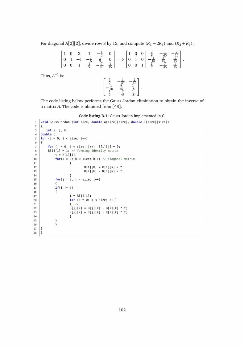
For diagonal A[2][2], divide row 3 by 15, and compute (R1 − 2R3) and (R2 + R3).
1 0 2 1 −13 0
0 1 −1 −16
13 0
0 0 1 19 − 7
45115
=⇒
1 0 0 79 − 1
45 − 215
0 1 0 − 118
845
115
0 0 1 19 − 7
45115
.
Thus, A−1 is:
79 − 1
45 − 215
− 118
845
115
19 − 7
45115
.
The code listing below performs the Gauss Jordan elimination to obtain the inverse ofa matrix A. The code is obtained from [48].
Code listing B.1: Gauss Jordan implemented in C.
1 void GaussJordan (int size, double A[size][size], double I[size][size])2 {3 int i, j, k;4 double t;5 for (i = 0; i < size; i++)6 {7 for (j = 0; j < size; j++) B[i][j] = 0;8 B[i][i] = 1; // forming identity matrix9 t = R[i][i];
10 for(k = 0; k < size; k++) // diagonal matrix11 {12 B[i][k] = B[i][k] / t;13 R[i][k] = R[i][k] / t;14 }15 for(j = 0; j < size; j++)16 {17 if(i != j)18 {19 t = R[j][i];20 for (k = 0; k < size; k++)21 { //22 B[j][k] = B[j][k] - B[i][k] * t;23 R[j][k] = R[j][k] - R[i][k] * t;24 }25 }26 }27 }28 }
102

Appendix C
Using HW/SW Co-designImplementation on Zynq Platform
This tutorial describes the setup steps for HW/SW codesign implementation of spectralclustering on ZedBoard development platform. The tutorial includes project creation,block design generation, simulation, synthesis and usage of Xilinx SDK Environmentfor interaction between software and hardware modules. In this tutorial, Xilinx Vivadov2019.1 (64-bit) is used.
C.1 Create Project
Open Vivado Design Suite and click on Create Project, a new project Wizard will popup. Click next and select the Project location as the folder downloaded from GitHubrepository available at [50]. The VHDL folder contains all necessary VHDL files, VHDLtestbenches, and Tcl scripts required for Vivado Design Suite project setup. Click nextand check on "Do not specify sources at this time" under "RTL Project" and then clicknext. Choose the Boards tab and locate "Zedboard Zynq Evaluation and DevelopmentKit". Using the Tcl Console, run project_SpectralClustering.tcl script by typing source pro-ject_SpectralClustering.tcl on the console. This will recreate the project. The project is setto xc7z020clg484-1 part number corresponding to Zedboard Zynq Evaluation and De-velopment Kit board. First, the script will include all source files, IP repositories, defaulttiming constraints, and simulation files. The Tcl script will also set design_1_wrapper astop module.
C.2 Synthesis and Simulation
Under IP Integrator, click on Open Block Design to view the synthesized block diagramof the whole project design. The provided Tcl scripts create instances, set properties, andcreate interface and the necessary port connections between corresponding IPs withinthat block diagram. Figure C.1 shows the generated HW/SW co-design synthesized blockdiagram. Simulation files are provided for in the Simulation Sources folder of the Project.Chooses one of the sources as top-level for simulation by Settings −→ Simulation −→Simulation top module name. An example waveform generated is shown in Figure C.2.
103
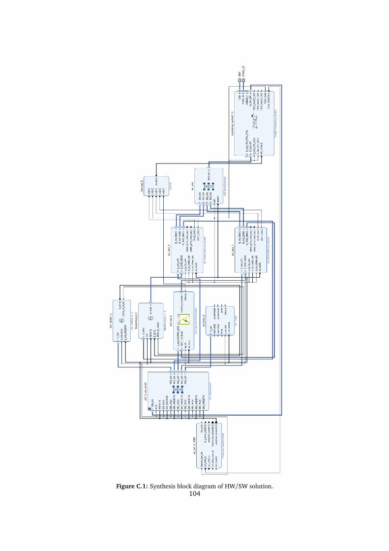
Figure C.1: Synthesis block diagram of HW/SW solution.104
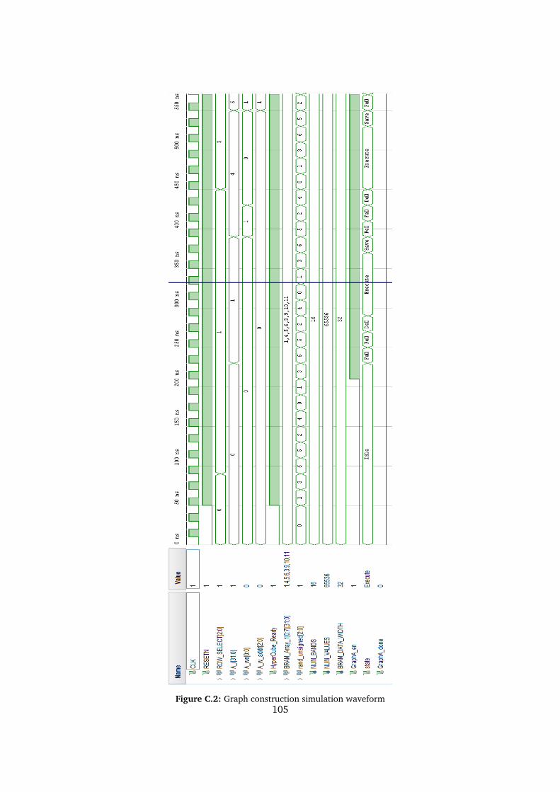
Figure C.2: Graph construction simulation waveform105
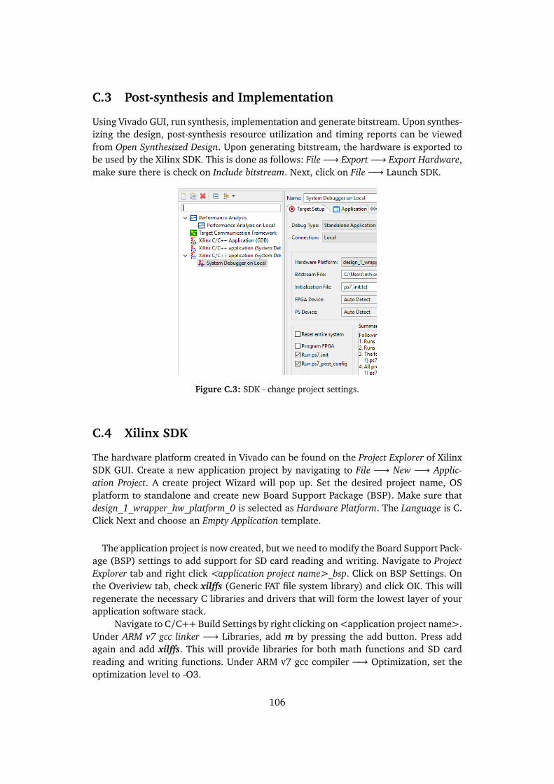
C.3 Post-synthesis and Implementation
Using Vivado GUI, run synthesis, implementation and generate bitstream. Upon synthes-izing the design, post-synthesis resource utilization and timing reports can be viewedfrom Open Synthesized Design. Upon generating bitstream, the hardware is exported tobe used by the Xilinx SDK. This is done as follows: File −→ Export −→ Export Hardware,make sure there is check on Include bitstream. Next, click on File −→ Launch SDK.
Figure C.3: SDK - change project settings.
C.4 Xilinx SDK
The hardware platform created in Vivado can be found on the Project Explorer of XilinxSDK GUI. Create a new application project by navigating to File −→ New −→ Applic-ation Project. A create project Wizard will pop up. Set the desired project name, OSplatform to standalone and create new Board Support Package (BSP). Make sure thatdesign_1_wrapper_hw_platform_0 is selected as Hardware Platform. The Language is C.Click Next and choose an Empty Application template.
The application project is now created, but we need to modify the Board Support Pack-age (BSP) settings to add support for SD card reading and writing. Navigate to ProjectExplorer tab and right click <application project name>_bsp. Click on BSP Settings. Onthe Overiview tab, check xilffs (Generic FAT file system library) and click OK. This willregenerate the necessary C libraries and drivers that will form the lowest layer of yourapplication software stack.
Navigate to C/C++ Build Settings by right clicking on<application project name>.Under ARM v7 gcc linker −→ Libraries, add m by pressing the add button. Press addagain and add xilffs. This will provide libraries for both math functions and SD cardreading and writing functions. Under ARM v7 gcc compiler −→ Optimization, set theoptimization level to -O3.
106

Next, navigate to Run −→ Run Configurations and double click on Xilinx C/C++application (System Debugger). System Debugger settings will be pop up as in FigureC.3. Make sure that Reset entire system and Program FPGA are unchecked as in the Fig-ure. Navigate to the Application tab and click check on ps7_cortexa9_0 processor. Thiswill enable a user to compile any further edited C code (for exmaple, edit user definedparameters) before execution on Zedboard. Press close.
Copy the C files from the Github repository [50] to<application project name> onthe Project Explorer. main.c file runs the program which reads the data from SD card,pre-processes the data, and initiates transfers using two different AXI DMA cores. Thedesign is ready to run. Click on Program FPGA to upload the bitstream on the FPGAdevice and then navigate to Run −→ System Debugger on Local and click Run.After all the execution of k-means clustering, the program reports the execution timeand writes the results to a file on SD card. The results can then be plotted on Python.
107

NTN
UN
orw
egia
n U
nive
rsity
of S
cien
ce a
nd T
echn
olog
yFa
culty
of I
nfor
mat
ion
Tech
nolo
gy a
nd E
lect
rical
Engi
neer
ing
Dep
artm
ent o
f Ele
ctro
nic
Syst
ems
Mas
ter’s
thes
is
Mohamed Ismail
HW/SW Co-design Implementation ofHyperspectral Image Classification Algorithm
Master’s thesis in Embedded Computing Systems
Supervisor: Milica Orlandic
June 2020
Copyright © 2022 FDOKUMEN