Frame Bundle of Riemannian Path Space and Ricci Tensor in Adapted Differential Geometry

Journal of Functional Analysis 177, 219�253 (2000)

Frame Bundle of Riemannian Path Space andRicci Tensor in Adapted Differential Geometry

Ana-Bela Cruzeiro

Gru� po de F@� sica-Matematica, Universidade de Lisboa, Av. Prof. Gama Pinto 2,1649-003 Lisbon, Portugal

and

Paul Malliavin

10 rue Saint Louis en l 'Isle, 75004 Paris, France

Communicated by Paul Malliavin

Received May 20, 2000; accepted May 20, 2000

dedicated to daniel w. stroock

The vanishing of the renormalized Ricci tensor of the path space above a Ricciflat Riemannian manifold is discussed. � 2000 Academic Press

Key Words: path space; infinite dimensional Riemann geometry; Weitzenbo� ckformula; heat semigroup.

Contents

Introduction.1. Frame Bundle and Absolute Differential Calculus on Path Space.2. Structural Equation of the Frame Bundle.3. Weitzenbo� ck Formula on the Path Space of a Ricci Flat Manifold.4. Tensorial Formulae of Integration by Parts.5. Towards Heat Semi-group on Adapted Vector Fields.Appendix

INTRODUCTION

Path Space has to be considered as some kind of ``amphibious animal''that must be fitted to live inside two different worlds: the world ofstochastic analysis and the world of infinite dimensional differentialgeometry. This joke has for corollary that, as far as possible, efficientdefinitions on Path Space must proceed simultaneously from these two dif-ferent worlds: to be efficient the connection has to be Markovian; in the

doi:10.1006�jfan.2000.3634, available online at http:��www.idealibrary.com on

2190022-1236�00 �35.00

Copyright � 2000 by Academic PressAll rights of reproduction in any form reserved.

same way efficient Ornstein�Uhlenbeck process has to be adapted, whichmeans that the projections defined by the canonical filtration of the PathSpace must be preserved during the OU evolution. There exists two defini-tions of the OU process on Path Spaces, one by Driver and Ro� ckner [4],the other by Norris [8]; only the Norris process satisfies this adaptnessprerequisite.

In their cooperation on the construction of Path Space theory, stochasticanalysis must play the role of the queen and differential geometry the roleof the servant: indeed only stochastic analysis can provide the renormalisa-tions, which are so vital for any infinite dimensional differential geometry.Differential geometry as developed in [2] fits the Norris paradigm only inthe case where the base Riemannian manifold is Ricci flat. This assumptionof Ricci flatness will be made in Sections 3�5.

Renormalization could mean replacing divergent series by stochasticintegrals, as is the case in [2]. In our setting renormalization will mean therestriction of classical identities, as the Weitzenbo� ck formula, to adaptedvector fields. This restriction will induce dramatic simplification offormulae of classical differential geometry such as those computed in [2].

The main result of this paper is the following: through this renormaliza-tion by restriction the Shigekawa�Ricci tensor associated to the Markovianconnection of Riemannian Path Space becomes equal to the identity, a resultwhich can be interpreted as the vanishing of the Ricci tensor itself. We haveobtained in [2, formula (9.7.1)], a similar statement at a formal level; inthe present work this statement means an effective Weitzenbo� ck formulavalid for adapted vector fields. The foundations of renormalization byrestriction have been set in [1]. At a conceptual level, this paper showsthat infinitesimal differential geometry on Path Space, started in [2], hasnow reached its maturity, making it possible to develop highlysophisticated computations leading nevertheless to simple results. TheMarkovian connection has been introduced in [2] where it appears as auseful tool to differentiate stochastic integrals; its legitimacy is reinforcedby the results established in this paper.

1. FRAME BUNDLE AND ABSOLUTE DIFFERENTIALCALCULUS ON PATH SPACE

Above a Riemannian manifold V of dimension d the bundle of all itsorthonormal frames O(V ) admits as a group of automorphisms the groupof orthogonal matrices SO(d ). In the infinite dimensional case the corre-sponding object will be the group of all unitary transformations of aHilbert space, which is much too large a group. We shall use the paradigmof adaptedness to squeeze it to a more manageable situation.

220 CRUZEIRO AND MALLIAVIN

We consider the Hilbert space H :=H1([0, 1], Rd). This Hilbert spacehas a continuous family of projectors 6_ , _ # [0, 1], defined by

d{(6_z) :=1[0, _]({) z* ({).

Going from the Hilbert space to its associated Segal probability space (cf.[7, Chap. 1]), the family of projectors 6_ corresponds to the Ito filtrationN_ .

We denote by U the group of unitary transformations of H commutingwith the family of projectors 6_ . We denote by Endres(H) the group ofbounded linear transformations of H commuting with the family ofprojectors 6_ .

1.1. Theorem. Denoting respectively by GL(d) and O(d) the lineargroup and the orthogonal group operating on Rd and denoting by P+(V) thecorresponding bounded measurable maps of [0, 1] into the correspondinggroup,

U&P+(O(d)) through the action (u V z)({) :=|{

0u(*) z* (*) d*,

and under the same action

Endres(H)&P+(GL(d)).

The Lie algebra of the group U can be identified to P+(so(d))=: G.We call an isometric surjective map from H onto the Cameron�Martin

tangent space T 1p(Pm0

(M )) a frame at the point p # Pm0(M ).

The parallel transport defines the canonic frame at p by the formula

z [ Z where Z{ :=t p{ � 0(z({)).

We have considered in [2] the inverse of this map under the notation 3p ,which we called the parallel form of Pm0

(M ); with a shorthand notation thecanonic frame is 3&1

p .We call adapted frame a frame which intertwins the projection operators

6* , this projection operator being defined on T 1p(Pm0

(M )) by

(6*(Z ))({) :=Z{ , \{<*; (6* Z )({)=t p{ � *(Z*), \{>*.

We define the frame bundle O(Pm0(M )) (shorthand as O) as the collection

of all adapted frames.

221RICCI TENSORS ON PATH SPACE

1.2. Theorem. The map

/: U_Pm0(M) [ O(Pm0

(M )) defined by(1.2) i

/(u, p): z [ 3&1p (u V z), \z # H,

is a bijective isomorphism. We denote as _ the section of the bundle ofadapted frames defined by _( p) :=/(e, p), where e denotes the constant pathequal to the identity. We denote by .: O(Pm0

(M )) [ Pm0(M ) the canonic

projection; then . b _ is the identity map on Pm0(M ).

Fixing u # U, we define

Qu : O [ O defined by r [ r b u&1, (1.2) ii

then Q*

defines a group action of U on O.

Proof. Obvious.

Markovian Connection on the Frame Bundle

We have introduced in [2] a Markovian connection and its asssociatedcovariant derivative {; this connection satifies the prerequisite of adapted-ness in the sense of [1]:

If Zi , Z2 are two adapted vector fields on Pm0(M ), then {Z1

Z2 is anadapted vector field.

Given z # H and given p # Pm0(M ), the Christoffel symbol of the

Markovian connection computed in [2] is

(1z, p V v){=|{

01z, p(*) v* (*) d*, where

(1.3) i

1z, p({) :=|{

00(z(*), odp(*));

then the martingale part of 1z, p belongs to G, meaning that the Markovianconnection preserves the Riemannian metric induced by the Hilbertianstructure of H.

The Markovian connection defines a family of canonic horizontal vectorfields on the frame bundle. We associate to z # H a vector field Az onO(Pm0

(M )) in the following way: using the section _ defined in 1.2, wedefine

Az(_( p)) :=\ dd= |==0

exp(&=1z, p), 3&1p (z)+ . (1.3) ii


At a generic point r=_( p) b u with u # U, we define Az(r) :=(1� z(r), Z� (r)) by

1� z(_( p) u) :=u&1 bd

d= |==0

exp(&=1u V z, p) b u; (1.4) i

Z� (r)=r(z). (1.4) ii

Proposition 1.6 constitutes the justification of the above definition (1.4).Given a vector field Z on Pm0

(M ) we call the H-valued function FZ

defined on the frame bundle by FZ(r) :=r&1(Z.(r)) its scalarization thisfunction satisfies the equivariance property

FZ(r b u)=u&1(FZ(r)) or FZ b Qu=u b FZ . (1.5)

Proposition. The Markovian covariant derivative {ZY is expressed onthe frame bundle by

F{r (z) Y (r)=(dFY , Az) r . (1.6)

Proof. Consider r=_( p) b u, then

FY (r) :=u&1FY (_(.(r))).

Take in particular u=u0 b exp =%, where % # G and where r0=_( p) u0 , inthis case

dd===0

FY (r0 exp(=%))=&% V FY (r0).

Taking %=&u&10 1u0 V zu0 we get

=u&10 1u0 V z(FY b _).

It remains to study the action of the horizontal component of Az which isequal to r(z). We define r==_( p+=r(z)) b u0 , where u0 # U is fixed:

dd===0

FY (r=)=u&10 Dr(z)(FY b _).

Therefore

(dFY , Az) r=u&10 3p({r(z)Y)=r&1({r(z) Y ); r=_( p) b u0 .

Tensorial Analysis

In classical differential geometry, a tensor field on a manifold V ismanipulated as the data in any local chart of a system of functions � i1 , ..., iq

j1 , ..., js,


each index running into [1, dim(V )]. The number q of superior indices iscalled the order of contravariance and the number s of inferior indices iscalled the order of covariance, the tensor field being of type (q, s). Bychange of local chart the covariant and contravariant indices transformaccording to distinct rules in duality with each other. As in the Path Spacethis local chart approach does not seem manageable, we do not need toexplicitly write here these classical change of chart rules.

The covariant derivative {i has the effect of adding a lower (covariant)index. Assume that V is a Riemannian manifold; the Christoffel symbolsare denoted 1 i

j1 , j2. The covariant derivative of a tensor of type (1, 0) (i.e.,

a vector field) is defined by

({j�)i :=Dj �i+:j1

1 ij, j1

� j1.

Imposing the property that the covariant derivative acts as a derivation onthe tensor algebra, we obtain for a (2, 0) tensor field the formula

({j�) i1 , i2=D j�i1 , i2+:j1

1 i1j, j1

� j1 , i2+1 i2j, j1

�i1 , j1, (1.7)

and so on for a (q, 0) tensor field. We emphasize the fact that the Christoffelsymbol acts on each indices of the considered tensor field.

1.8. Definition. We call the data on O of a family of functionals

8;1 , ..., ;q:1 , ..., :s

: O [ L2([0, 1]q+s; R), ;*

, :*

# [1, d] (1.8) i

satifying the equivariance property

8(Qu(r))({1 , ..., {q+s)

=(u({1)� } } } �u({q)� u({q+1)� } } } � u({q+s)) 8(r)({1 , ..., {q+s)

(1.8) ii

\{ # [0, 1]q+s, where u :=u* denotes the transpose of u, which is alsoequal to u&1 a tensor field of type (q, s) on Pm0

(M); for instance in the caseof a (2, 0) tensor field the equivariance is

(8(Qu(V)));1 , ;2 ({1 , {2)= ::1 , :2

u;1:1

({1) u;2:2

({2) (8:1 , :2)({1 , {2). (1.8) iii

By equivariance a tensor field is fully known by its restriction to the rangeof the canonic section _.


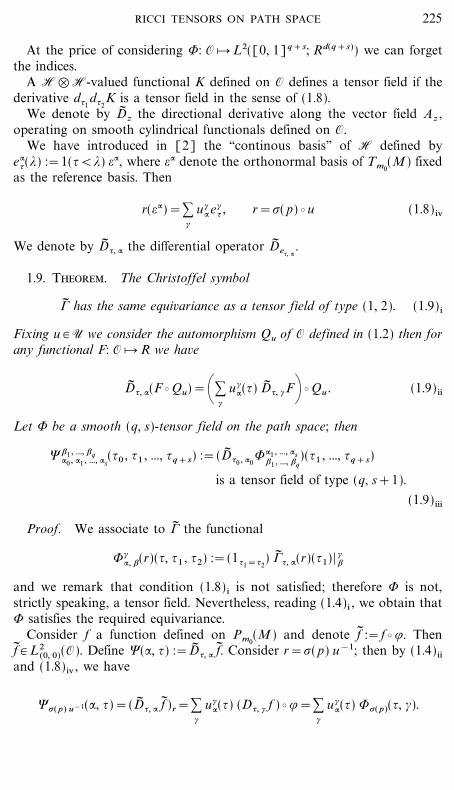
At the price of considering 8: O [ L2([0, 1]q+s; Rd(q+s)) we can forgetthe indices.

A H�H-valued functional K defined on O defines a tensor field if thederivative d{1

d{2K is a tensor field in the sense of (1.8).

We denote by D� z the directional derivative along the vector field Az ,operating on smooth cylindrical functionals defined on O.

We have introduced in [2] the ``continous basis'' of H defined bye:

{(*) :=1({<*) =:, where =: denote the orthonormal basis of Tm0(M ) fixed

as the reference basis. Then

r(=:)=:#

u#:e#

{ , r=_( p) b u (1.8) iv

We denote by D� {, : the differential operator D� e{, :.

1.9. Theorem. The Christoffel symbol

1� has the same equivariance as a tensor field of type (1, 2). (1.9) i

Fixing u # U we consider the automorphism Qu of O defined in (1.2) then forany functional F: O [ R we have

D� {, :(F b Qu)=\:#

u#:({) D� {, #F+ b Qu . (1.9) ii

Let 8 be a smooth (q, s)-tensor field on the path space; then

9 ;1 , ..., ;q:0 , :1 , ..., :s

({0 , {1 , ..., {q+s) :=(D� {0 , :08:1 , ..., :s

;1 , ..., ;q)({1 , ..., {q+s)

is a tensor field of type (q, s+1).

(1.9) iii

Proof. We associate to 1� the functional

8#:, ;(r)({, {1 , {2) :=(1{1={2

) 1� {, :(r)({1)| #;

and we remark that condition (1.8) i is not satisfied; therefore 8 is not,strictly speaking, a tensor field. Nevertheless, reading (1.4)i , we obtain that8 satisfies the required equivariance.

Consider f a function defined on Pm0(M ) and denote f� :=f b .. Then

f� # L2(0, 0)(O). Define 9(:, {) :=D� {, : f� . Consider r=_( p) u&1; then by (1.4) ii

and (1.8) iv , we have

9_( p) u&1(:, {)=(D� {, : f� )r=:#

u#:({) (D{, # f ) b .=:

#

u#:({) 8_( p)({, #).


We get an equivariance of type u*, which means that D� {, : f� behaves as atensor field of type (0, 1). K

Consider now the case where 8 is a tensor field of type (1, 0). Then,according to (1.4)i the vertical component of D� {0 , : acts on 8, at the point_( p) u&1, as

(18)(_( p) u&1)=(u1u&1 V z) 8(_( p) u&1).

Using the linearity of 1z relative to z it is sufficient to study the case wherez=e{

:; then the identity

u V e{:=:

#

u:#({) e#

{

implies, since u&1=u*, that

1u&1 V e{, :=:

#

u#:({) 1{, # . (1.9) iv

taking in account (1.9)ii we get for the indice of covariant derivative anequivariance of type u*, that is altogether a tensor field of type (1, 1). K

Absolute Differential Calculus

Definition. The covariant derivative {{, : of a tensor field 8 is definedby

({{, :8)p=(D� {, :8)_( p) . (1.10)

Formula (1.6) insures that this definition is coherent with the definition ofthe covariant derivative of a vector field.

Theorem. For a tensor 8 of type (q, s)

({{, :8)p (*1 , ..., *q , *q+1 , ..., *q+s)

=D{, :(8_( p))+ :1� j�q

1{, :(*j) 8_( p)(..., *j } } } )

& :q<i�q+s

1{, :(*i) 8_( p)(..., * i } } } ) (1.11) i

The calculus on 8 of a monomial in derivatives D�*

is reduced to covariantderivatives according to the formula

(D� {1 , :1} } } D� {k , :k

8)_( p)=({{1 , :1} } } {{k , :k

8)p . (1.11) ii


Remark. The formula (1.11) i extends to our setting formula (1.7).

Proof. The equivariance replaces the derivation in the direction of thevertical component of D� {, : by multiplication by the infinitesimal matrices

exp(=1{, :)

for the contravariant components and for the covariant components by

(exp(=1{, :))*=exp(&=1{, :),

the last equality being a consequence of the fact that 1{, : # U. We finishthe proof by differentiating with respect to = and taking ==0. K

Consider the case of a monomial of degre 2; denote by D� {2 , :28 :=9 a

function defined on O which has the variance of type (q, s+1). It is there-fore a tensor of type (q, s+1). It is determined by its restriction to therange of _ which is equal to {{2 , :2

8; it is possible to construct from {{2 , :28

a tensor field 3 having the variance (q, s+1). Of course we have3=D� {2 , :2

8 from the characterization of a tensor field as its restriction tothe range of the canonic section. This double notation emphasizes that 3can be effectively constructed starting only from the data of {{, : 8.

We have D� {1 , :19={{1 , :1

3 on the range of _, and we get (1.11) ii . K

Matricial Notations

For subsequent computations it will sometimes be necessary to have afull grasp of the indices of matrices. For this purpose we shall use theChristoffel symbol in the developed notation as in [2, formula (7.4.1)],

1 #:; ;({; *)=1({<*) |

*

{0:, $, ;, #odx$ (1.12) i

In matricial notation the passage from contravariant tensor to covariantindices transfer upper indices into lower indices. This exchange of indicessends the matrix 1 #

V, ;(V) into its transpose, which changes its sign. There-fore in the matricial notations the minus sign appearing in the last term ofthe r.h.s. of (1.11) disapears. Consider for instance a (1, 1) tensor field8`

= ({1 , {2):

({{, :8)`= ({1 , {2)=D{, :(8`

=)+1 #:; =({, {1) 8`

#+1 `:; #({, {2) 8#

= . (1.12) ii

Derivation of Trace Operator. Given two tensor fields 8 and 9 of type(1, 0) and (0, 1), their trace is defined by

trace**

(8�9 )=::

8:9: ; (1.12) iii


then this trace is a tensor field of type (0, 0);

D{, ; ::

8:9:=::

({{, ;8): 9:+8:({{, ;9 ): ; (1.12) iv

Writing {{, ;=D{, ;+1{, ; , this formula comes from the fact that thecovariant derivative on contravariant indices is equal to minus thecovariant derivartive on covariant indices. Formula (1.12)iv takes the sym-bolic form

D{, ;(trace**

(8�9 ))=trace **

(({{, ;8)�9+8�{{, ;9 ). (1.12)v

2. STRUCTURAL EQUATION OF THE FRAME BUNDLE

This section will show that absolute differential calculus can lead tosimpler computations than the brute force approach; for instance, compare(2.7) and (2.8) with parallel computations made in [2].

We define a parallelism on O by the data on O of a 1-differential form ?with values in H_U. We denote by ?* its first component and by ?� itssecond component, which are defined as

(T , ?* ) r :=r&1(.$(r)(T )), (T , ?� ) r :=1� ?* (T )+�$(r) T, (2.1)

where � denotes the projection on the first factor of the domain of /defined in (1.2), and where the tangent space at the point u # U has beenidentified to u exp(=G).

We remark that the vector fields Az defined in (1.4) are constant vectorfields in this parallelism satisfying

(Az , ?* ) =z, (Az , ?� ) =0. (2.2)

Theorem. The action of Qu on the parallel form ? preserves the decom-position (?* , ?� ) and has the following expression:

Qu* ?* =u b ?* , Qu* ?� =u b ?� b u&1. (2.3)

Proof. We recall that the definition of the reciprocal image of differen-tial forms Qu* is given by the identity

(Qu*?, T ) r=(?, Q$u(r) Tr) Qu(r) ,


valid for any vector field T. We have

. b Qu=. therefore .$(Qu(r)) b Q$u(r)=.$(r) or

(.$(Qu(r))(Q$u(r) Tr)=(.$(r))(Tr);

finally

(Qu* ?* , T ) r=ur&1(.$(Qu(r))(Q$u(r)(Tr))=u((?* , T ) r). K

We split ?� =?1+?2 where ?2=1� ?* (T ) ; then

(Qu* ?2, T ) r=((1� (Qu(r)))?* ((Q$u(r) T ) .

According to the first equation of (2.3) we have ?* (Q$u(r))=u(?* (T )),which means a variance of type (1, 0); as 1

*is covariant in the lower index

these two variances annihilate each other and we get that ?2 has a varianceof type (1, 1). That is, it satisfies the second equation of (2.3). K

It remains to deal with ?1; we have

?1r (Tr)=(�(r))&1 d

d= |==0

�(r+=Tr)

(Qu*?1, T ) r=?1Qu(r)(Q$u(r) Tr)

=u(�(r))&1 dd= |==0

�(Qu(r+=Tr))

=u?1r (Tr) u&1 K

The structural equation of the frame bundle consists in the expression ofthe parallelism of the coboundary of the parallel differential form. AsQu* d?=dQu* ?, we deduce from (2.3) that

Qu*(d?* )=u(d?* ), Qu*(d?� )=u(d?� ) u&1.

According to these relations it is sufficient to compute these coboundary onthe range of the canonic section _.

Theorem.

((T1 7 T2 , d?* )+?� (T1) ?* (T2)&?� (T2) ?* (T1))_( p)

:=T=&|0

* 0(?* (T2), ?* (T1)) odx; (2.4)


in the case where the Ricci tensor of M vanishes in the r.h.s. of (2.4) we canreplace the Stratonovitch integral by an Ito integral written with the sameintegrand.

The second structural equation is

((T1 7 T2 , d?� )&?� (T1) ?� (T2)+?� (T2) ?� (T1))_( p)

=&[1z , 1z$]&(Dz1z$)+(Dz$ 1z)+1[z, z$] where (2.5)

z=?* (T1), z$=?* (T2).

Proof. For any vector fields Ti we have the identity

(d? , T1 7 T2)=&(?, [T1 , T2]) +DT1(?(T2))&DT2

(?(T1)). (2.5) i

Taking the vector fields constant in the parallelism (i.e., ?(Ti)=constant),this identity reduces the computation of the coboundary to the computa-tion of the bracket.

Given %i # G, consider the constant vertical vector fields

?* (Ti)=0, ?� (Ti)=%i i=1, 2; then

(DTiF )(r)=

dd= |==0

F(Qexp(&=%i )(r))). (2.5) ii

The Lie bracket on U is equal to the Lie bracket on G according to thefollowing identity:

exp(&=%1) exp(&=%2)&exp(&=%2) exp(&=%1)= 12=2[%1 , %2]+o(=2).

As Q*

is a group action on O this action preserves the Lie bracket;therefore

([T1 , T2], F ) r=d

d= |==0

(F(Qexp(=[%1 , %2])(r)).

according (2.5) ii we obtain

?([T1 , T2])=(0, &?� (T1) ?� (T2)+?� (T2) ?� (T1));

as the r.h.s. of (2.5) vanishes, we get the structural equation for two verticalvectors fields. K

Consider now the case of two horizontal vector fields: ?� (Ti)=0, i=1, 2and fixing z1 , z2 # H constant, we define Ti by the relation ?* (Ti)=zi ; thenTi=D� zi

. The identity (2.5) i reduces the proof of the structural equation to


the computation of [D� z1, D� z2

]; as we are on the range of the canonicsection _, according (1.11) ii this bracket is equal to [{z1

, {z2].

Given 8`, { a tensor field of type (1, 0), we have

{z$8=Dz$ 8+1z$ V 8.

We shall explicate the action of 1z$ on 8`, { by the expresssion

1 `# (z$, {) 8#, { :=(1z$ V 8)`, {.

Then

({z{z$8)`=I1, 2+II1, 2+III1, 2+IV1, 2+V1, 2 where

I1, 2=(DzDz$&D1z V z$)(8`),

II1, 2=1 `#(z$, {)(Dz8)#+1 `

#(z, {)(Dz$8)#,

III1, 2=(Dz1z$) V,

IV1, 2=&11zz$ ,

V1, 2=1z V 1z$ V.

As II1, 2 is symmetric in the indices (1, 2), it does not contribute; as

I1, 2&I2, 1=([z, z$]&1zz$+1z$z, d(8`))=&DT(8`)

the last identity resulting from the structural equation of [2, formula(6.2.1)];

[{z , {z$]=&DT&1T+(Dz1z$)&(Dz$1z)&11z z$+11z$ z+[1z , 1z$];

(2.5) iii

using the facts

&DT=&{T+1T , T&1zz$+1z$ z=&[z, z$]

we obtain

[{z , {z$]=&{T+(Dz1z$&Dz$ 1z)+[1z , 1z$]&1[z, z$] , (2.5) iv

which by (2.5) i proves the structural equation in the case ?� (Ti)=0,i=1, 2. K


The last case of the structural equation to check is when ?� (T1)=0 and?* (T2)=0. Then there exists %2 # G such that (2.5) ii holds true and we have

[T2 , T1]=d

d= |==0

(Qexp(&=%2))*T1 ;

as Qu acts on H by the rotation u* we find [T2 , T1]=%2 V z1 . K

Theorem. The torsion of the Markovian connection is

T (z, z$) :={zz$&{z$z&[z, z$]=&|0

* 0(z, z$) odx. (2.6)

The curvature of the Markovian connection is given by

R(z, z$) :=&?� ([{z , {z$])=&[1z , 1z$]&(Dz1z$)+(Dz$1z)+1[z, z$] .

(2.7)

If Ricci(M )=0 the Ricci type trace of the curvature vanishes:

Trace R :=::

|1

0R(z, e:

{) V e:{ d{=0. (2.8)

Proof. The computation of the torsion is a direct consequence of thestructural equation [2, formula (6.2.1)], as already pointed out in[2, formula (9.2.2)]. Reading (2.5) we get (2.7).

The vanishing of the Ricci tensor for terms not containing derivativesresults from

[1z , 1e{:] e:

{=0; 1T (z, e{:)e:

{=0, 11e{:ze:

{=0, 11ze {: e:

{=0.

For the computation of Dz1*

we take z=e;* .

Then the derivative D*, ;1e{:=0 if *>{. For *<{ the third term of the

curvature gives rise inside the trace to

::

D{, : 1*, ;e:{=1(*<{) :

:

0;, :, :, V( p({))=&1(*<{) Ricci*; ( p({))=0.

For *>{ this term is

D{, :1*, ;e:{=0.


3. WEITZENBO� CK FORMULA ON THE PATH SPACEOF A RICCI FLAT MANIFOLD

Starting from this section until the end of this paper we shall make thepermanent assumption that M is Ricci flat. This does not imply that thecurvature tensor of M is trivial (see for instance Beauville, J. DifferentialGeometry 18 (1983), 755�782).

We have on the Path Space Pm0(M ) two natural OU processes, intro-

duced respectively by Driver and Ro� ckner and by Norris; both processesare reversible for the canonic Wiener measure + defined on Pm0

(M ). In thecase where M is Ricci-flat, these two processes coincide.

Kazumi [5] gave the following expression of the generator of the Norrisprocess:

2= 12 :

:|

1

0D2

{, : d{&D{, :odx:({). (3.1) i

The meaning of the Stratonovitch integral appearing here is clarified in(3.1) iii when we apply 2 to a cylindrical functional. In the non-cylindricalcase formula (3.5)i has to be considered a formal abridged notation.

We call the data of a finite set S/]0, 1] a mesh. A smooth cylindricalfunction f based on the mesh S=[{i] can be witten as f ( p)=F( p(({1), ..., p({n)); then

D{, : f = :0<i�n

1({<{i) ci, :( f ) where ci, :( f )=(=: | t p0 � {i

(�i F )).

It follows from this formula that the derivation vectors on cylindrical func-tions based on the mesh S :=[{i] have dn components. We denote by L2

S

the finite dimensional subspace of L2([0, 1]; Rd) constituted by the func-tions which are continuous and locally constant in the complement of S.Then the L2 norm induces on L2

S a structure of euclidean space. We takeas basis of these derivation vectors the vectors z:

k defined by the twoproperties

z* :k # L2

S ; z:k ({i)==: $k

i .

Direct computation shows that

z* :k=\ 1

{k&{k&1

1[{k&1 , {k]&1

{k+1&{k1[{k+1&{k]+ =:;


then ci, :( f )=Dzi: f. Denote y:

s =1[0, {s]=:; then (z* :

k | y;s )=$:

; $ sk which

means that z* **

and y**

are dual basis in L2S ; therefore for every , # L2

S wehave

,=:k:

y:k(, | z* :

k).

As ( y:i | y;

j )={i 7{j $:; we deduce

&,&2L2

S= :

i, j, :

{i 7 {j (, | z* :i )(, | z* :

j ), \, # L2S . (3.1) ii

In particular the Dirichlet form of Driver and Ro� ckner for cylindrical func-tions f, g associated to same mesh has the polarized expression

D( f, g)=E \::

|1

0D{, : f D{, : g d{+=:

:

:i, j

{i 7 {j E(Dzi: f Dzj

: g)

Using [2, formula (1.5.2)] we have for every smooth functional , the for-mula of integration by parts

E(Dz,)=E((z* | 9* x) ,), \z satisfying z* # L2S ,

where 9x is a continuous function, linear in S c and equal on S to x.Therefore

E(Dzi: f Dzj

: g)=&E( fDzi: Dzj

: g)+E( f (z* :i | 9* x) Dzj

: g).

Multiplying by {i 7 {j and summing together we get D( f, g)=&E( f2g),where

22g= ::, i, j

{i 7 {j Dzi: Dzj

: g& ::, i, j

{i 7{j (z* :i | 9* x) Dz: g (3.1) iii

the first order term can be written

I :=& :i, j, :

( y:i | y:

j )(9* :x | z* :

i )(dg | z* :j )

where dg # L2S is defined by (dg){=D{ g # L2

S . by applying (3.1) ii we get theKazumi formula:

I :=&(9* x | dg)Ls2=&:

:|

1

0D{, : g odx:({) K


The lifted Laplacian is the differential operator defined on O by

(2� )r := 12 :

:|

1

0D� 2

{, : d{&D� {, : odx:u({), (3.1) iv

where

x:u({)=|

{

0u:

#(*) dx#(*), r=Qu(_( p)).

We shall give below a precised signification of the Stratonovitch integralappearing in this definition. But before we shall deduce a formal propertyfrom a formal definition.

Proposition. For every smooth function F on O and every u # U we have

2� (F b Qu)=(2� F ) b Qu (3.1)v

Given f a smooth function on Pm0(M ), we have

2� f� =(2f ) b . (3.1)vi

More generally, if 8 is a tensor field of type (q, s), then 2� 8 is a tensor fieldof type (q, s).

Proof. We split 2� into its first order term and its second order term.According to (1.9) ii the second derivative D� {, :D� {$, :$ has an equivarianceunder Qu of type (0, 2). Then

�:, :1(r)=D� {, :D� {, :1

has the following equivariance:

�:, :1(Qu(r))= :

#, #1

u#:({) u#1

:1({) �#, #1

(r)

Taking now :=:1 and making a summation on : we get

::

�:, :(Qu(r))= :#, #1

\::

u#:({) u#1

: ({)+ �#, #1(r)

we remark that by the orthogonality of u the term (*) is equal to $#1# . K


It remains to consider the first order term. Then xu has an equivarianceof type (1, 0) when D� {, : has the equivariance (0, 1); therefore

::

D� {, : odx:u({)

is invariant under Qu . K

We remark that f� is invariant under the action of Qu*. According to (2.1) i

we have that 2� f� is invariant by Qu*; therefore it is sufficient to compute iton the range of _ where the identity is obvious. K

We shall limit ourselves to the action of 2� on a tensor field 8 of type(q, s). According to (3.1)v it is sufficient to compute 8 on the range of thecanonic section _.

A tensor field 8 of type (q, s) is called cylindrical if 8 b _ is a cylindricalfunctional on Pm0

(M ) taking its values in H�q� (H*)�s; then for a cylin-drical tensor field 8 we shall compute (2� 8)(_( p)) by the formula (3.1) iii .As 2� 8 is a tensor field of type (q, s)) it is fully determined by its restrictionon the range of _; therefore the formal notation (3.1) iv leads to an effectivedefinition on the dense subspace of cylindrical tensor field. K

By Bianchi identities, in the integral (1.3) defining the Christoffel symbol1z , the Stratonovitch differential can be replaced by an Ito stochasticdifferential. The same fact holds true for integral (2.6) defining the torsionT. We deduce the basic fact

Theorem. Given Zi two adapted vector fields, define the vector field

T (Z1 , Z2)({) :=&|{

00(Z1 , Z2) dx; (3.1)vii

then for every smooth functional F we have

E(DTF )=0. (3.1)viii

Proof. Apply [2, formulas (2.5.5) and (2.3.5)]; see [1] for identitiesrelated to (3.1)viii . K

If ! is a semi-martingale process whose Ito differential is d{!=a:; dx;+c: d{, and a:;+a;:=0, we have the following

Theorem. For every smooth cylindical function F on the Wiener space,

(D!F )=E \F |1

0c: dx:+


Proof. The martingale part of the process ! defines a measure-preservingisomorphism, since the diffusion coefficient is an antisymmetric matrix.

Theorem. Given a vector field Z let z :=3(Z ); then for all smoothcylindrical functions f, we have

E \:;

|1

0({*, ; 2� f� ) z* ;(*) d*+=E \:

;|

1

0(D*, ; 2f ) z* ;(*) d*+ . (3.2)

Proof. According to (3.1)vi

2� f� =(2f ) b .

therefore the l.h.s. has no vertical component and its covariant derivative{*, ; is equal to D*, ; . K

Theorem. Given an adapted vector field Z we have the identity

|O \:

%|

1

0[2� (D� {, *

f� )]{, % z* % ({) d{+ d+~ =E(DZ 2f )+E(DZ( f )). (3.3)

Remark. The covariant derivative involves derivation and mutiplicationby operators # G. These operations do not change the continuous indices {but operate on the discrete indices (:, %) as appearing in the notation of (1.8).This operation is expressed on the l.h.s. of (3.3) by a free index symbolizedas

*.

Proof. Granted (3.2), the r.h.s. of (3.3) is equal to an integral on O

relative to the measure +~ :=_*

+; therefore the identity (3.3) is reduced tocommutations on the frame bundle and finally, according to (1.11)ii , tocommutations of covariant derivatives. By formal calculation

D� 2*, ; D� {, :&D� {, : D� 2

*, ;=&A&B where

A :=2[D� {, : , D� *, ;] D� *, ; , (3.4)

B :=[D� *, ; , [D� {, : , D� *, ;]],

these identities leading to corresponding identities for covariant derivatives.A basic fact is the orthogonality of A to any adapted vector field accordingto the following lemma:


Main Lemma. Fix the continuous index (*, ;). Then for any adaptedvector field Z and any smooth functional f we have

E \::

|1

0([{{, : , {*, ;] {*, ; f� ) z* :({) d{+=0. (3.5)

Proof . We fix (*, ;); then by using (2.5) iii

[{{, : , {*, ;]=&DT+[1{, : , 1*, ;]+D{, :1*, ;&D*, ;1{, :&1U , (3.5) i

where U=1{, :(e;*)&1*, ;(e:

{). As f� is a tensor of type (0, 0) we have{*, ; f� =D*, ; f.

As M is Ricci flat we have

T!({, :)=&1(!>sup({, *)) |!

sup({, *)0:, ;, #, $ dx$. (3.5) ii

Let g=D*, ; f; then the first term of the r.h.s. of (3.5) i can be written as &Jwhere

J :=E \::

|1

0(DT ({, :) g) z* :({) d{+ .

As g is smooth we know that g is Skorohod�Nualart�Pardoux�Zakai(SNPZ)-integrable (cf. Appendix). Using [2, formula (2.3.9)] we have for({, :) fixed DT ({, :) g=9{, :(1), where

9{, :(\) :=1(\>sup({, *)) :#, $

|\

sup({, *)(D!, # g) V (0:, ;, #, $ dx$(!)),

and where V denotes the SNPZ anticipative integral defined in theAppendix. As Z is an adapted vector field, we have

J=::

E \|1

09{, :(1) z* :({) d{+=0. K

By adaptedness we have 1*, ; V e;*=0 and 1*, ; V a V e*, ;=0 for all

a # Endres(H1).

Therefore the second term of the r.h.s. of (3.5)i has a vanishing contribution.


The third term of (3.5) i is treated remarking that D*, ; 1{, :e;* vanishes if

*>{ or if *<{ and remarking that

(D{, : 1*, ;) e;*=1({=*) 0;, :, ;, *

,

an expression which vanishes a.e. in { (because * is fixed) and thereforedoes not contribute to the integral in {.

It remains to deal with the fourth term of (3.5) i , that is, 1U V e;*

Then we must have that support(U ) & [0, *[ is non-empty. This is neverthe case for 1{, : e;

* . The remaining possibility is 1*, ;e:{ if {<* but then the

Christoffel symbol 1*({)=0. K

3.6. Proof the Theorem. The term B in (3.4) is a first order differentialoperator, only ?* ((B) operates on df� .

Reading (3.5) i we have

?* ([{{, : , {*, ;])=&T, (3.6) i

?� ([{{, : , {*, ;])=[1{, : , 1*, ;]+D{, : 1*, ;&D*, ;1{, :&1U+1T . (3.6) ii

As we compute the bracket on O of the non-constant vector field (&T, 0)with the constant vector field e*, ; the structural Eq. (2.5), (2.6) has to becorrected by adding the derivation of the composants in the parallelism ofthe non-constant vector field. This derivation is given by the expression,where ({, :) is fixed,

K := &D*, ;T!({, :)=1(!>sup({, *)) \D*, ; |!

sup({, *)0:, ;, #, $ dx$+ ;

we use now the derivation formula of an Ito integral given in [2, formula(7.6.4)], (under its simplified form coming from the Ricci flatnesshypothesis):

K=0:, ;, #, ;( p(*))+1(!>sup(({, *)) |!

sup({, *)M:, ;, #, $ dx#;

M:, ;, #, $ :=({*, ;0):, ;, #, $ .

When we compute commutation with 2� , we must make a summation onthe index ;; this implies the vanishing of the first term by Ricci flatness.Using the expression given in [2, formula (7.1.1)] for the Markoviancovariant derivative, we get that M

*is adapted and antisymmetric in the

indices (#, $). The contribution of this derivative to (3.3) is, using again the


representation by a SNPZ integral of the directional derivative along atangent process according to [2, formula (2.3.9)], given by

E \::

|1

0z* :({) _|

1

sup({, *)(D!, # f ) V (M:, ;, #, $ dx$(!))& d{+ . (3.6) iii

By the adapteness of Z we can replace the bracket by EN{([V])=0. K

Therefore the calculus of B can be done from (3.6) i , (3.6) ii using only thestructural equations.

We split B=B1+B2 where

B1 &?* ([e;* , ?* ([{{, : , {*, ;])]), B2 &?* ([e;

* , ?� ([{{, : , {*, ;])])

We write the term B1 under the shape (3.6) iii using the representation usingan SNPZ integral

B1=E \|1

0 _|1

sup(*, {)(D!, # f ) V (0;, $, #, `T!, $({, :) dx` (!)))& z* :({) d{+ ;

(3.6) iv

the upper limit 1 for the integral inside the [V] can be changed into { bythe effect of conditional expectation EN{([V]), admissible by the adapted-ness of z; we have !�{, but according to (3.5) ii we have then T!=0 for!�{ and (3.6) iv vanishes. K

The terms in B2 come from the infinitesimal action of the verticalcomponents acting as infinitesimal rotations on e;

*; we have made thesecomputations in the proof of the main lemma: for instance,D*, ;1{, :(e;

*)=0.The only new term to consider is, where ({, :) is a fixed parameter,

1T (e{, *)=|1

01!(e;

*) 0(e:{ , e;

*) odx(!);

in order to get a non-vanishing integrand we must have simultaneously!<* and !>* and therefore this integral also vanishes identically.

Putting all the previous computations together we have obtained:

the identity (3.3) holds true for the second order term order terms in 2� .

It remains to deal with the first order term of order 2� . We fix (*, ;); twoterms C and D appear, where

C=E \|1

0 _|1

0(D!, = f ) V (0=, $(e:

{ , e;* , e=

! , dx$(!))& z* :({) d{+ ;


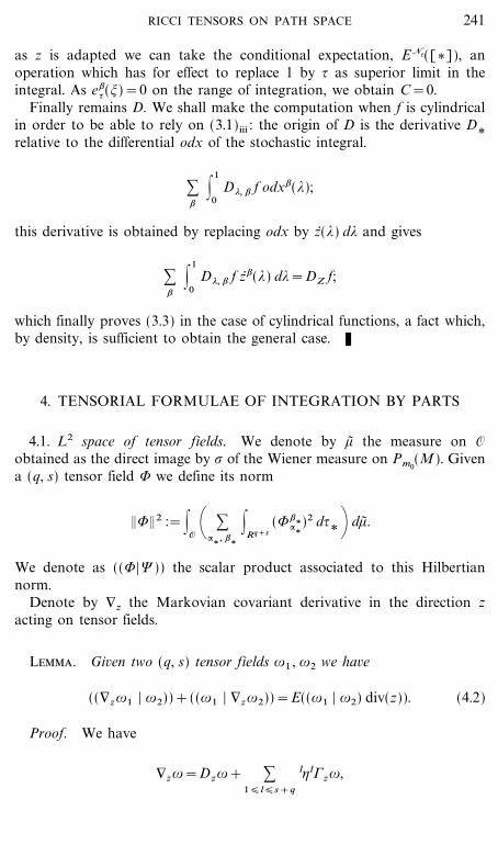
as z is adapted we can take the conditional expectation, EN{([V]), anoperation which has for effect to replace 1 by { as superior limit in theintegral. As e;

{(!)=0 on the range of integration, we obtain C=0.Finally remains D. We shall make the computation when f is cylindrical

in order to be able to rely on (3.1) iii : the origin of D is the derivative D*

relative to the differential odx of the stochastic integral.

:;

|1

0D*, ; f odx;(*);

this derivative is obtained by replacing odx by z* (*) d* and gives

:;

|1

0D*, ; f z* ;(*) d*=DZ f;

which finally proves (3.3) in the case of cylindrical functions, a fact which,by density, is sufficient to obtain the general case. K

4. TENSORIAL FORMULAE OF INTEGRATION BY PARTS

4.1. L2 space of tensor fields. We denote by +~ the measure on O

obtained as the direct image by _ of the Wiener measure on Pm0(M ). Given

a (q, s) tensor field 8 we define its norm

&8&2 :=|O \ :

:*

, ;*

|Rq+s

(8;*:*)2 d{

*+ d+~ .

We denote as ((8|9 )) the scalar product associated to this Hilbertiannorm.

Denote by {z the Markovian covariant derivative in the direction zacting on tensor fields.

Lemma. Given two (q, s) tensor fields |1 , |2 we have

(({z|1 | |2))+((|1 | {z|2))=E((|1 | |2) div(z)). (4.2)

Proof. We have

{z|=Dz|+ :1�l�s+q

l'l1z|,


where l'=1 or l'=&1 according to the contravariance or the covarianceof the index. As 1z is antisymmetric,

(1 �z |1 | |2)+(|1 | 1 �

z |2)=0.

Therefore

(({z|1 | |2))+((|1 | {z|2))=E(Dz(|1 | |2))=E((|1 | |2) div(z)) K

4.3. Theorem. Suppose that M is a Ricci flat manifold, consider theDirichlet form on L2

(q, s) tensor field defined by

D(8, 8)=&3&2L2

(q, s+1),

where 3 :={*

8. Consider the polarized expression

D(8, 9 )=|O \:

:|

1

0({{, :8 | {{, : 9 ) d{+ d+~ ; (4.3) i

then we have

D(8, 9 )=&|O

(8 | 2� 9 ) d+~ (4.3) ii

Remark. According to (3.1) iv 2� 9 is a tensor of type (q, s); therefore thescalar product (8 | 2� 9 ) is well defined.

Proof. As we integrate relative to the measure +~ , we are in the range of_ and we can replace D� {, : by {{, : . Then, denoting 9{, : :={{, :9, we haveby (4.2)

D(8, 9 )=::

|1

0E(({{, :8 | {{, :9 )) d{

=::

|1

0E(&(8 | {2

{, :8) d{+(8 | {{, :8) odx:({)),

an identity coming from the fact that div(D{, :)=odx:({), formal proofwhich can be substantiated along the lines of (3.1) iii . K

4.4. Corollary. For two smooth tensor field 81 , 82 of same type (q, s)we have

((2� 81 | 82))=((81 | 2� 82))


Proof. The r.h.s. is equal to D(8, 9 ), an expression which is obviouslysymmetric in 8, 9. K

The Duality Coupling. In order to define a duality coupling between atensor field 8 of type (q, s) and a tensor field 9 of type (s, q), we introducethe following preliminary operations:

(i) making the tensor product 3 :=8�9 we obtain a tensor fieldof type (l, l )) where l=q+s;

(ii) to a tensor field 3 of type (l, l ) we associate its trace Tr(3) whichis the tensor field defined by

(Tr(3))(r)= :#1 , ..., #l

|[0, 1]l

9 #1 , ..., #l#1 , ..., #l

(r)({1 , ..., { l , {1 , ..., {l) d{1 } } } d{l.

We have (Tr(3)(Qu(r))=(Tr(3)(r), relation which means that Tr(3) isa tensor of order (0, 0).

We define the duality coupling

(8, 9) :=Tr(8�9 ); ((8, 9))=|O

(8, 9) r +~ (dr).

Remark. We have defined in (1.12) the operation trace which consistsin taking only sum on indices situated in lower and upper position. Thenew operation Tr could be decomposed in a two-step operation: firstrealize the operation trace and second integrate on the diagonal of thecontinuous variables {i .

The Star Operation. We associate to a tensor field 9 of type (s, q) thetensor field 9* of type (q, s) defined by the identity

((8 , 9)) =((8 | 9*)).

Definition. We define an elliptic operator 2� on tensor fields by

2� 9=(2� 9*)*.

Proposition. Given two smooth tensor fields 8, 9 respectively of type(q, s) and of type (s, q) we have

((2� 8, 9)) =((8, 2� 9)) (4.5)

Proof

((2� 8, 9)) =((2� 8 | 9*))=((9 | 2� (9*)))=((8 , 2� 9)) .


4.6. Proposition. Let {� z9 :=({z9*)*; then for a vector field Y onPm0

(M) we have

{� zY=DzY&1zY

and on the support of _ we have

2� Y= 12 \:

:|

1

0{� 2

{, :&{� {, : odx:({)+ Y.

Proof . Formal computation.

Remark. Using the matricial notations introduced in (1.12) the proof of(4.6) becomes almost tautological. A vector field Z is given by its com-ponents z:({). The differential form |=Z* is defined by its components|:({)=z:({). According to (1.11) the covariant derivative acts on |

*(({)

by the factor &1, which proves (4.6).

Main Theorem. We introduce the differential operator L on vectorfields, defined by

L= 12 :

:|

1

0{� 2

{, : d{&|1

0{� {, : odx:({). (4.7)

If Z is an adapted vector field, then LZ is an adapted vector field. (4.8)

For every adapted vector field and every smooth functional f we have theintertwinning formula

E((d2f, Z) )+E((df, Z) )=E((df, LZ) ) (4.9)

Proof. Granted (3.3) the l.h.s. of (4.9) is equal to the bilinear form

B(Df, Z ) :=|O \:

%|

1

0[2� D{, *

f� ]{, % z* % ({) d{+ d+~

Our strategy will consist in extending this bilinear form to a tensorial set-ting; we denote by L2

0, 1(O) the space of (0, 1) tensor fields; then 8df :=D� f�is a (0, 1) tensor field. Then, denoting by 9Z the tensor field associated toZ we have

B(Df, Z )=((2� 8df , 9Z));

we conclude by using (4.5). K

Remark. The general strategy of the proof of the main theorem hasbeen to separate the algebraic identities treated in Sections 2 and 3 from


the integration by part which is dealed through a symmetrization using aDirichlet form approach. The symmetrization procedure is out of the ques-tion to be applied in the algebraic part: in fact only constant functions haveadapted differentials!

5. TOWARDS THE HEAT SEMI-GROUP ON ADAPTEDVECTOR FIELDS

First we shall recall and amplify the construction done in [6] of the heatsemi-group above a d-dimensional compact Riemannian manifold V, whichwill be assumed, in order to simplify the notations, Ricci flat. We denoteby O(V ) its orthonormal frame bundle; the Levi�Civita connection definesd canonic horizontal vector fields Ak , k # [1, d] on O(V ) and the horizon-tal diffusion is parametrized by a d-dimensional brownian motion xk

through the Stratonovitch SDE:

drx(t)=:k

Ak (rx(t)) odxk (t).

We associate to a 1-differential form | defined on V the family of d scalar-valued functions defined by

Fk (|, r) :=(r(=k), |.(r)) , k # [1, d],

where =*

is the canonic basis of Rd. Denote by &21 the de Rham�HodgeLaplacian acting on 1-differential forms.

Theorem. The solution of the Cauchy problem for the heat equation

�|t

�t=21|t , |0=| given, (5.1) i

has the following expression:

Fk (|t , r0)=Erx(0)=r0(Fk (|, rx(t))). (5.1) ii

Proof. See [7].

The Coprocess

We want to construct the dual semi-group of the semi-group on 1-differ-ential forms defined by (5.1) ii . In the scalar case it is well known that thedual of a semi-group operating on functions is a semi-group operating onprobability measures.


In our case we introduce the convex set of probability measure M on thetangent bundle. The Ito stochastic parallel transport is defined by

txt � 0(z) :=rx(t) b r&1

0 (z), where z # T.(r0)(V ).

It can be shown that the parallel transport is independent of the choice ofthe frame r0 # .&1(/(z)) where /: T(V ) [ V.

We define a semi-group 6t on M by

|T(V )

U(z) d(6t \) :=E$(U(txt � 0(z)))

for any bounded test fuction U defined on T(V ).We consider Ma/M consisting of measures \ which are of the form

_*

& where & is a probability measure on V and where _ is a section ofT(V ).

We define a projection Q: M [ Ma in the following way: given \ # M wedenote & :=/

*\; we disintegrate \ along / by

\=|V

*v &(dv),

where *v is a probability measure supported by /&1(v)=Tv(V ).We define a section

_(v) :=|Tv(V )

z*v(dz)

and we define Q($ :=_*

&. To a 1-differential form % on V we associate thefunction F% defined on T(V ) by

F% (z) :=(z, %/(z)) .

Then the projection Q is characterized by the property

|T(V )

F% d\=|T(V)

F% dQ(\)

holding true for all 1-differential forms %.

5.2. Proposition. Given \ # Ma, define

6 at (\) :=Q(6t (\)); (5.2) i


then the transformation 6 at : Ma [ Ma satisfies the semi-group property

6 at b 6 a

t$=6 at+t$ . (5.2) ii

Proof . The parallel transport is a linear transformation which preservesthe barycenter of a probability measure.

Proposition. Consider |t , a family of differential 1-forms dependingupon the parameter t satisfying the heat equation (5.1) i ; then write6 a

t (\)=(_t)*&t and denote as Zt the vector field defined by _t ; then

|V

(|t , Z0) d&0=|V

(|0 , Zt) d&t . (5.3)

Proof. By linearity it is sufficient to prove this formula in the casewhere &0 is the Dirac mass at the point v0 . Then taking _0 satisfying_0(v0)=r0(=k), formula (5.3) results from (5.1)ii .

Proposition. Denote by + the invariant probability measure for thelaplacian on V, that is the riemannian volume. To any vector field Z weassociate the measure \Z # Ma defined as (_Z)

*+. Then 6 a

t (\Z) # Ma,denote by (Zt , +) its decomposition. Define Pt (Z )=Zt . Then Pt is a semi-group and its infinitesimal generator is given by

(2� Z)(v0)= lim' � 0

'&1Ev0((tvy

' � 0)* (Zvy('))&Zv0). (5.4)

Proof. Using the semi-group property it is sufficient to study the infini-tesimal increase of the process at time t=0. The coprocess constructionleads to a conditionnal expectation upon the final value

Z'(v1)=E vx(')=v1(tvx' � 0(Z0(vx(0))).

We reverse the Brownian motion on V from the time ' relatively tothe invariant measure + defining vy(s)=vx('&s). As the measure + isreversible, the reversed process has the same law as the original process.Conditionning by the final value becomes conditionning by the initial valuefor the process vy . Finally, by the unitarity of the parallel transport,

T vx' � 0=(T vy

' � 0)*.

Remark. The transpose changes the sign of covariant derivatives as thisappeared in (4.6).


The Infinite Dimensional Case

5.5. Lemma. Given Y, Z two vector fields on Pm0(M), the covariant

derivative for the Markovian connection satisfies

(d{({ZY ))( p0)=DZ exp&1p0({)(d{Y),

where expp0({) is the normal chart of M of center p0({) and where

d{Y= lim' � 0

'&1(t p{ � {+'(Y({+')&Y({)).

Proof [2, formula (7.1.1)]. The Norris process [8] is a M-valued twoparameters process pw(t, {), t>0, { # [0, 1] such that t [ pw(t, *) realizesthe trajectory of the OU process leaving the measure + invariant.

We shall make the following fundamental assumption which presumablywill need the full Norris machinery in order to be firmly established.

5.6. Assumption. For all fixed {0 the map t [ pw(t, {0) is a M valuedsemi-martingale, depending continously from {.

Given a section %0 : [0, 1] [ O(M ) such that .(%({))= p0({), we con-sider its deformation %t defined by the condition that for all {0 fixed, thecurve t [ %t ({0 ) is the lifting to O(M ) through the Levi�Civita� connectionof the semi-martingale defined in (5.2).

5.7. Theorem. Suppose assumption (5.6) is established and take for %0

the parallel transport t p0

* � 0 . Then define the holonomy map t [ uwt # U by

uwt (z* )=(t pt

w)&1 b %t b t p

0w(z* ) (5.7) i

then

_( pwt ) b ut

is the process lifted to O through the Markovian connection.

5.8. Theorem. Suppose assumption (5.6) established; then, given anadapted vector field Z on Pm0

(M ), define

P� t (Z )( p0)=exp(&t) Epw(0)= p0((uw

t )* (Zpw(t))) (5.8) i

(5.8) ii If Z is an adapted vector then P� t (Z ) is an adapted vector field.

ddt |t=0

P� tZ=2� Z (5.8) iii


Denote by Pt the OU semi-group defined on functions on Pm0(M); then for

any smooth function f and any adapted vector field we have

|Pm0

(M )(d(Pt f ), Z) d+=|

Pm0(M )

(df, P� t Z) d+ (5.8) iv

|Pm0

(M )(d(Pt f ), Z) d+=|

Pm0(M )

(P� t (df ), Z) d+, where(5.8)v

(P� t (|))p0=exp(&t) Epw(0)= p0

(uwt (|pw(t))).

Given a functional f defined on Pm0(M ), denote

Da{, : f =E N{(D{, : f ); (5.8)vi

then

(Da{, :(Pt f ))( p0)=exp(&t) Ep0

(u#:(w, t, {)((Da

{, : f )( pw(t)))),

where u(w, t, {0) denotes the matrix describing the parallel transport for theLevi�Civita� connection of M of the frame t p

{, 0(=*

) along the curve on Mdefined by t [ pw(t, {0).

Proof. Property (5.8) i results from the the fact that the parallel trans-port is an adapted operation. K

For Property (5.8) ii we shall follow [1]. Fix Z adapted; then \� smoothwe define

At (�) :=E((dPt�, Z)&(d�, P� t (Z)) ).

Remark that A0(�)=0. Differentiating relative to t, we get

A4 t (�)=E((dPt (2�), Z)&(d�, 2� (Zt)) ),

where Zt=P� tZ. As Zt is adapted we can apply (3.3) combined with (4.6),

E((d�, 2� Zt)&(d2�, Zt) )=0

and we get the identity

A4 t (�)=At (2�).

Fix � and t0>0 and define

Nt=At (Pt0&t (�)), t # [0, t0].

Then N4 t=0 and N0=0 which implies that 0=Nt0=At0

(�).


Formula (5.8)v is deduced from (5.8) iv by making first an interchange ofintegration and expectation, second a transposition, and finally again aninterchange of expectation and integration.

We write now (5.8)v expliciting the duality coupling a differential formwith a vector field. As Z{ is adapted we can project for the Ito filtrationand we get

0=E \::

|1

08{, :Z{, : d{+

where

8({, :) :=EN{(D{, :(Pt ( f ))&(P� t D{, *f ){, : )

Fixing t and f, it is legitimate to choose Z{, :=8({, :), a choice whichimplies 8({, :)=0 and proves (5.8)vi . K

APPENDIX

The purpose of this Appendix is to prove A3 , a proof which could beobtained in two lines by cross-reference to [2]. Because of its crucial usein Section 3 above, we prefer to provide below a leisurely written proof. Inthis Appendix we shall also introduce several new stochastic integralswhich will disappear in the final statement, A3 .

We take as a probability space X the Wiener space of the brownianmotion on Rd. We denote by ` a scalar-valued martingale defined on X.Given a scalar-valued process u

*its Skorohod�Stratonovitch and

Skorohod stochastic integrals relative to `, namely

|1

0u{od`({), and |

1

0u{ V d`({),

are defined as the limit of the Nualart�Pardoux�Zakai sums

:i

M$i(u) `($ i) and :

i

E $ic(M$i

(u)) `($i),

where $i denote the intervals of a finite partition of [0, 1] in intervals,where E$ i

cdenotes the conditional expectation constituted by averaging

relative to the _-field generated by x({)&x({i), $i=[{i , {i+1], { # $ i , `($i)=`({i+1)&`({i) and where

M$(u)=|$|&1 |$

u{ d{


denotes the mean of u on the interval $. To have unambiguous notationswe have introduced * in the notation for the Skorohod integral; thenotation � a dx will be used for the Ito integral of adapted processes.

A1 Assume that f # D1+02 (X ), a*

*# L�&0(X; L2[0, 1]) and assume that

a**

is adapted and that a:;+a;

:=0; then if one of the two stochastic integralsbelow exits, the other exists as well and

|1

0(D{, : f ) V d`:({)=|

1

0(D{, : f ) od`:({),

where

`:({)=|{

0a:

; dx;.

The difference between the two integrals is given by the following limitof Nualart�Pardoux�Zakai sums:

:i

(E $ic(M$i

(D* , : f ))&M$i

( f )) `:($i).

Using the Clark�Ocone formula, this expression is equal to

&:i \M$i |

$i

EN*(D2

*, #; * , : f ) dx#(*)+ `:($i).

By the Wiener identity on the quadratic variation of the Brownian motion,the limit when the mesh of the partition goes to zero is equal to

&lim :i, #

|$i

M$i(D2

*, #; * , : f ) a:#(*) d*,

an expression which tends to zero granted the symmetry of the secondderivatives and the antisymmetry of a*

*. K

A proof of the existence of the integral relative to *d` could bereconstructed by resuming the methodology of Nualart�Pardoux in thisextended context; this construction leads to the inequality

} |1

0u V d` }�cp &u&Dp

1.

A2 Given a martingale ` having for Ito differential d`=c: dx: and suchthat the coefficients c: are semi-martingales having for Ito differentials


dc:=c:; # dx#+c:; 0 d{, for any process u*

# D�&01 (X; H ), the two integrals

below exist and are equal:

|1

0u V d`=:

:|

1

0(c:u) V dx:.

Write the Nualart�Pardoux sums of the two sides of this equality. Onthe LHS we shall approximate `($i) by c:({i) x:($ i); the legitimacy of thisapproximation on the LHS comes from the majoration

E \}:i

&\:i +

approximated

}2

+�:i

|E$ icM$i

(u)|2 = i |$ i |,

where 0<=i<2 and =i � 0. After this first approximation the differencebetween the Nualart�Pardoux sums approximating the LHS and the RHScan be written as

:i

E$icM$i

(u*

(c:(V)&c:({i))) x:($i);

E$ ic(c:(*)&c:({i))=E$ i

c \|*

{i

c:; 0(t) dt+=O( |$i | ),

E$ic \\|$i

E N t(Dt, #u*) dx#(t)+\|

*

{i

c:; # dx#(t)+c:; 0(t) dt++=O( |$i | ).

These two contributions multiplied by x($i)=O( |$i |1�2&=) give a

contribution in |$i |3�2&=, expression which after summation on the indices

i tends again to zero. K

A3 Let f # D1+02 (X ). Assume that the matrix a:

; satisfies the hypothesisof A2 and furthermore that a:

; # D�&01 (X); then D` f exists and is equal to

D` f =:;

|1

0 \::

a:; D{, : f + V dx;({).

Fix a**

and denote D( f ) the difference between the LHS and the RHS.Granted A2 we have that |D( f )|�c & f &D

2� . By direct computation of the

Stratonovitch integral appearing in A1 we obtain D( f )=0 for all f smoothcylindrical functions; we conclude by a density argument. K


REFERENCES

1. A. B. Cruzeiro, S. Fang, and P. Malliavin, A probabilistic Weitzenbo� ck formula onRiemannian path, J. Anal. [Jeruzalem 2000]

2. A. B. Cruzeiro and P. Malliavin, Renormalized differential geometry on path space,structural equation, curvature, J. Funct. Anal. 139 (1996), 119�181.

3. A. B. Cruzeiro and P. Malliavin, Energy identities and estimates for anticipative stochasticintegrals on a Riemannian manifold, Stochast. Anal. Relat. Top. 42 (1998), 221�234.

4. B. Driver and M. Ro� ckner, Construction of diffusions on path spaces and loop spaces ofcompact riemannian manifolds, C.R. Acad. Sci. Paris Ser. I 320 (1995), 1249�1254.

5. T. Kazumi, Le processus d'Ornstein�Uhlenbeck sur l'espace des chemins et riemanniensle proble� me des martingales, J. Funct. Anal. 144 (1997), 20�45.

6. P. Malliavin, Formules de la moyenne, calcul de pertubations et the� ore� me d'annulationpour les formes harmoniques, J. Funct. Anal. 17 (1974), 274�291.

7. P. Malliavin, ``Stochastic Analysis,'' Grundlehren der Mathematik, Vol. 313, p. 342,Springer-Verlag, Berlin�New York, 1997.

8. J. R. Norris, Twisted sheets, J. Funct. Anal. 132 (1995), 273�334.9. D. Nualart and E. Pardoux, Stochastic calculus with anticipating integrands, Prob. Theory

Relat. Fields 78 (1988), 535�581.10. I. Shigekawa, The de Rham�Hodge�Kodaira decomposition on an abstract Wiener space,

J. Math. Kyoto Univ. 26 (1986), 191�202.11. D. W. Stroock, ``An Introduction to the Analysis of Paths on a Riemannian Manifold,''

Amer. Math. Soc. Surveys and Monographs, Vol. 74, p. 269, Amer. Math. Soc.,Providence, 2000.

Printed in Belgium


Frame Bundle of Riemannian Path Space and Ricci Tensor in Adapted Differential Geometry

Documents

Transcript of Frame Bundle of Riemannian Path Space and Ricci Tensor in Adapted Differential Geometry