BAFS: Bundle Adjustment With Feature Scale Constraints for ...

804 IEEE ROBOTICS AND AUTOMATION LETTERS, VOL. 3, NO. 2, APRIL 2018

BAFS: Bundle Adjustment With Feature ScaleConstraints for Enhanced Estimation Accuracy

Vladimir Ovechkin and Vadim Indelman

Abstract—We propose to incorporate within bundle adjustment(BA) a new type of constraint that uses feature scale information,leveraging the scale invariance property of typical image featuredetectors (e.g., SIFT). While feature scales play an important rolein image matching, they have not been utilized thus far for esti-mation purposes in a BA framework. Our approach exploits thealready-available feature scale information and uses it to enhancethe accuracy of BA, especially along the optical axis of the camerain a monocular setup. Importantly, the mentioned feature scaleconstraints can be formulated on a frame to frame basis and donot require loop closures. We study our approach in synthetic en-vironments and the real-imagery KITTI dataset, demonstratingsignificant improvement in positioning error.

Index Terms—Localization, mapping, SLAM.

I. INTRODUCTION

ACCURATE pose estimation and structure reconstructionare important in a variety of applications, including vi-

sion aided navigation (VAN) [10], simultaneous localizationand mapping (SLAM) [8], [16], visual odometry (VO) [4],augmented reality, structure from motion (SfM), tracking androbotic surgery. Bundle adjustment (BA) is a commonly usedapproach to address these and other related problems, and assuch, has been extensively investigated over the years; see [22]for an extensive review of different aspects in BA.

Standard BA approaches typically assume a pinhole cameramodel [9] and minimize re-projection errors between measuredand predicted image coordinates. This minimization is typicallyobtained using iterative nonlinear optimization techniques that,provided a proper initial guess, converge to the maximum aposteriori (MAP) solution over camera poses and landmarks thatrepresent the observed environment. Alternative formulationshave been also developed in recent years. These include, forexample, structureless BA approaches, such as Light BundleAdjustment (LBA) [11]–[15] that algebraically eliminate the3D points and minimize the residual error in multiple viewgeometry constraints. In contrast, dense BA approaches, suchas DTAM [19] and SVO [4], minimize the photogrammetricerrors for each overlapping image.

Manuscript received September 7, 2017; accepted December 5, 2017. Dateof publication January 11, 2018; date of current version January 25, 2018. Thisletter was recommended for publication by Associate Editor U. Frese and Edi-tor C. Stachniss upon evaluation of the reviewers’ comments. (Correspondingauthor: Vadim Indelman.)

V. Ovechkin is with the Technion Autonomous Systems Program,Technion—Israel Institute of Technology, Haifa 32000, Israel (e-mail: [email protected]).

V. Indelman is with the Department of Aerospace Engineering, Technion—Israel Institute of Technology, Haifa 32000, Israel (e-mail: [email protected]).

Digital Object Identifier 10.1109/LRA.2018.2792141

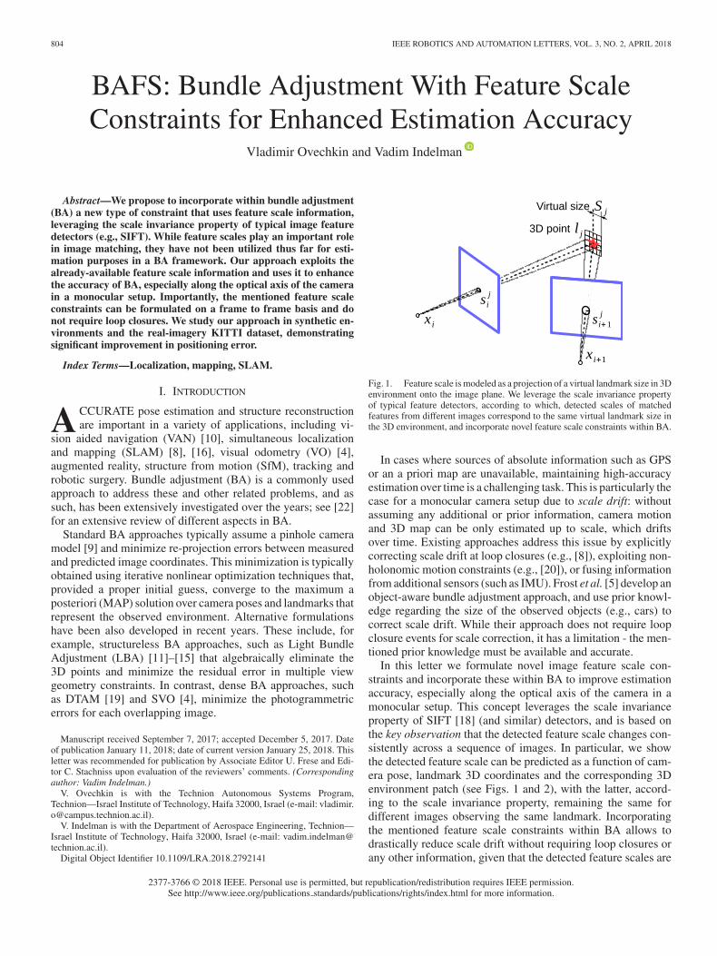
Fig. 1. Feature scale is modeled as a projection of a virtual landmark size in 3Denvironment onto the image plane. We leverage the scale invariance propertyof typical feature detectors, according to which, detected scales of matchedfeatures from different images correspond to the same virtual landmark size inthe 3D environment, and incorporate novel feature scale constraints within BA.

In cases where sources of absolute information such as GPSor an a priori map are unavailable, maintaining high-accuracyestimation over time is a challenging task. This is particularly thecase for a monocular camera setup due to scale drift: withoutassuming any additional or prior information, camera motionand 3D map can be only estimated up to scale, which driftsover time. Existing approaches address this issue by explicitlycorrecting scale drift at loop closures (e.g., [8]), exploiting non-holonomic motion constraints (e.g., [20]), or fusing informationfrom additional sensors (such as IMU). Frost et al. [5] develop anobject-aware bundle adjustment approach, and use prior knowl-edge regarding the size of the observed objects (e.g., cars) tocorrect scale drift. While their approach does not require loopclosure events for scale correction, it has a limitation - the men-tioned prior knowledge must be available and accurate.

In this letter we formulate novel image feature scale con-straints and incorporate these within BA to improve estimationaccuracy, especially along the optical axis of the camera in amonocular setup. This concept leverages the scale invarianceproperty of SIFT [18] (and similar) detectors, and is based onthe key observation that the detected feature scale changes con-sistently across a sequence of images. In particular, we showthe detected feature scale can be predicted as a function of cam-era pose, landmark 3D coordinates and the corresponding 3Denvironment patch (see Figs. 1 and 2), with the latter, accord-ing to the scale invariance property, remaining the same fordifferent images observing the same landmark. Incorporatingthe mentioned feature scale constraints within BA allows todrastically reduce scale drift without requiring loop closures orany other information, given that the detected feature scales are

2377-3766 © 2018 IEEE. Personal use is permitted, but republication/redistribution requires IEEE permission.See http://www.ieee.org/publications standards/publications/rights/index.html for more information.

https://orcid.org/0000-0002-1863-3442

OVECHKIN AND INDELMAN: BAFS: BA WITH FEATURE SCALE CONSTRAINTS 805

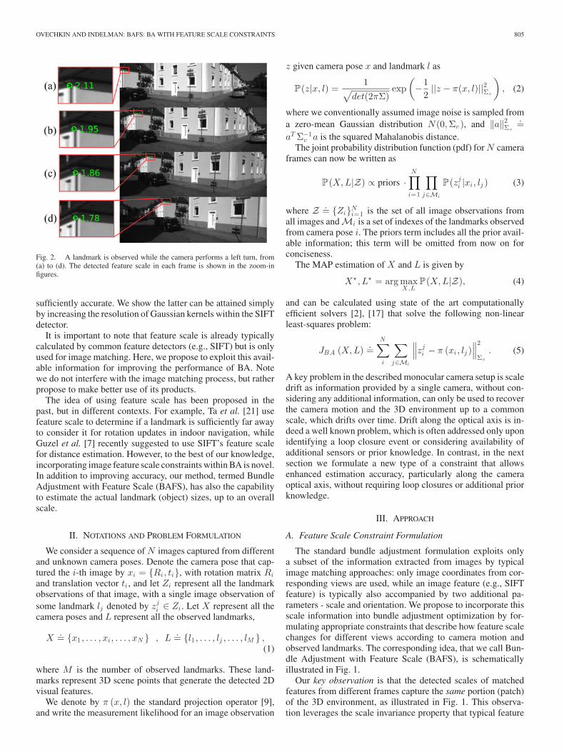
Fig. 2. A landmark is observed while the camera performs a left turn, from(a) to (d). The detected feature scale in each frame is shown in the zoom-infigures.

sufficiently accurate. We show the latter can be attained simplyby increasing the resolution of Gaussian kernels within the SIFTdetector.

It is important to note that feature scale is already typicallycalculated by common feature detectors (e.g., SIFT) but is onlyused for image matching. Here, we propose to exploit this avail-able information for improving the performance of BA. Notewe do not interfere with the image matching process, but ratherpropose to make better use of its products.

The idea of using feature scale has been proposed in thepast, but in different contexts. For example, Ta et al. [21] usefeature scale to determine if a landmark is sufficiently far awayto consider it for rotation updates in indoor navigation, whileGuzel et al. [7] recently suggested to use SIFT’s feature scalefor distance estimation. However, to the best of our knowledge,incorporating image feature scale constraints within BA is novel.In addition to improving accuracy, our method, termed BundleAdjustment with Feature Scale (BAFS), has also the capabilityto estimate the actual landmark (object) sizes, up to an overallscale.

II. NOTATIONS AND PROBLEM FORMULATION

We consider a sequence of N images captured from differentand unknown camera poses. Denote the camera pose that cap-tured the i-th image by xi = {Ri, ti}, with rotation matrix Ri

and translation vector ti , and let Zi represent all the landmarkobservations of that image, with a single image observation ofsome landmark lj denoted by zj

i ∈ Zi . Let X represent all thecamera poses and L represent all the observed landmarks,

X.= {x1 , . . . , xi , . . . , xN } , L

.= {l1 , . . . , lj , . . . , lM } ,(1)

where M is the number of observed landmarks. These land-marks represent 3D scene points that generate the detected 2Dvisual features.

We denote by π (x, l) the standard projection operator [9],and write the measurement likelihood for an image observation

z given camera pose x and landmark l as

P (z|x, l) =1

√det(2πΣ)

exp(−1

2||z − π(x, l)||2Σv

), (2)

where we conventionally assumed image noise is sampled froma zero-mean Gaussian distribution N(0,Σv ), and ‖a‖2

Σv

.=aT Σ−1

v a is the squared Mahalanobis distance.The joint probability distribution function (pdf) for N camera

frames can now be written as

P (X,L|Z) ∝ priors ·N∏

i=1

∏

j∈Mi

P (zji |xi, lj ) (3)

where Z .= {Zi}Ni=1 is the set of all image observations from

all images and Mi is a set of indexes of the landmarks observedfrom camera pose i. The priors term includes all the prior avail-able information; this term will be omitted from now on forconciseness.

The MAP estimation of X and L is given by

X�,L� = arg maxX,L

P (X,L|Z), (4)

and can be calculated using state of the art computationallyefficient solvers [2], [17] that solve the following non-linearleast-squares problem:

JBA (X,L) .=N∑

i

∑

j∈Mi

∥∥∥zji − π (xi, lj )

∥∥∥2

Σv

. (5)

A key problem in the described monocular camera setup is scaledrift as information provided by a single camera, without con-sidering any additional information, can only be used to recoverthe camera motion and the 3D environment up to a commonscale, which drifts over time. Drift along the optical axis is in-deed a well known problem, which is often addressed only uponidentifying a loop closure event or considering availability ofadditional sensors or prior knowledge. In contrast, in the nextsection we formulate a new type of a constraint that allowsenhanced estimation accuracy, particularly along the cameraoptical axis, without requiring loop closures or additional priorknowledge.

III. APPROACH

A. Feature Scale Constraint Formulation

The standard bundle adjustment formulation exploits onlya subset of the information extracted from images by typicalimage matching approaches: only image coordinates from cor-responding views are used, while an image feature (e.g., SIFTfeature) is typically also accompanied by two additional pa-rameters - scale and orientation. We propose to incorporate thisscale information into bundle adjustment optimization by for-mulating appropriate constraints that describe how feature scalechanges for different views according to camera motion andobserved landmarks. The corresponding idea, that we call Bun-dle Adjustment with Feature Scale (BAFS), is schematicallyillustrated in Fig. 1.

Our key observation is that the detected scales of matchedfeatures from different frames capture the same portion (patch)of the 3D environment, as illustrated in Fig. 1. This observa-tion leverages the scale invariance property that typical feature


detectors (e.g., SIFT [18]) satisfy. As an example, we considerthe image sequence shown in Fig. 2, where a single feature istracked and its detected scale across different images is explic-itly shown. One can note that, indeed, in all of the frames, thedetected scale represents an identical portion of the environ-ment, i.e., the contents inside of the circle with radius equals todetected scale is identical in all frames.

We shall consider the mentioned 3D environment patch extentas virtual landmark size and denote it for the jth landmark bySj . Based on the above key observation, we argue the detectedfeature scales in different images change consistently and canbe predicted. Specifically, letting sj

i denote the detected featurescale of the jth landmark in the ith image frame, and consideringa perspective camera, we propose the following observationmodel for sj

i

sji = f

Sj

dji

+ vi, (6)

where f is the focal length and vi is the measurement noisewhich is modelled to be sampled from a zero-mean Gaussiandistribution with covariance Σf s , i.e., vi ∼ N (0,Σf s). In (6)we use dj

i to denote the distance along the optical axis from thecamera pose xi to landmark lj . In other words, assuming theoptical axis is the z axis in the camera frame,

dji (xi, lj )

.= zc ,

⎡

⎢⎣

xc

yc

zc

⎤

⎥⎦ = Rilj + ti , (7)

where Ri and ti are the ith camera rotation matrix and translationvector, i.e., xi = {Ri, ti}.

We note one might be tempted to consider dji to be simply the

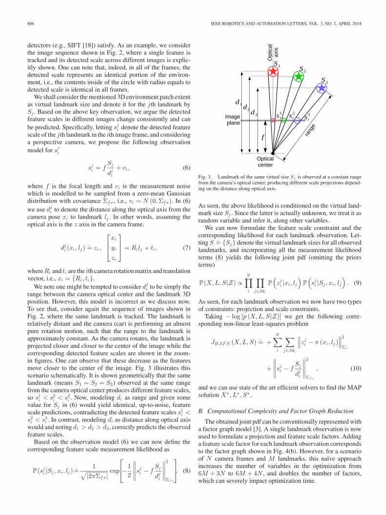
range between the camera optical center and the landmark 3Dposition. However, this model is incorrect as we discuss now.To see that, consider again the sequence of images shown inFig. 2, where the same landmark is tracked. The landmark isrelatively distant and the camera (car) is performing an almostpure rotation motion, such that the range to the landmark isapproximately constant. As the camera rotates, the landmark isprojected closer and closer to the center of the image while thecorresponding detected feature scales are shown in the zoom-in figures. One can observe that these decrease as the featuresmove closer to the center of the image. Fig. 3 illustrates thisscenario schematically. It is shown geometrically that the samelandmark (means S1 = S2 = S3) observed at the same rangefrom the camera optical center produces different feature scales,so s1

i < s2i < s3

i . Now, modeling di as range and given somevalue for Sj in (6) would yield identical, up-to-noise, featurescale predictions, contradicting the detected feature scales s1

i <s2

i < s3i . In contrast, modeling di as distance along optical axis

would and noting d1 > d2 > d3 , correctly predicts the observedfeature scales.

Based on the observation model (6) we can now define thecorresponding feature scale measurement likelihood as

P (sji |Sj , xi, lj )

.=1

√|2πΣf s |exp

⎡

⎣−12

∥∥∥∥∥sj

i − fSj

dji

∥∥∥∥∥

2

Σf s

⎤

⎦. (8)

Fig. 3. Landmark of the same virtual size Sj is observed at a constant rangefrom the camera’s optical center, producing different scale projections depend-ing on the distance along optical axis.

As seen, the above likelihood is conditioned on the virtual land-mark size Sj . Since the latter is actually unknown, we treat it asrandom variable and infer it, along other variables.

We can now formulate the feature scale constraint and thecorresponding likelihood for each landmark observation. Let-ting S

.= {Sj} denote the virtual landmark sizes for all observedlandmarks, and incorporating all the measurement likelihoodterms (8) yields the following joint pdf (omitting the priorsterms)

P (X,L, S|Z) ∝N∏

i

∏

j∈Mi

P(zj

i |xi, lj

)P

(sj

i |Sj , xi, lj

). (9)

As seen, for each landmark observation we now have two typesof constraints: projection and scale constraints.

Taking − log [p (X,L, S|Z)] we get the following corre-sponding non-linear least-squares problem

JBAF S (X,L, S) .= +N∑

i

∑

j∈Mi

∥∥∥zj

i − π (xi, lj )∥∥∥

2

Σv

+

∥∥∥∥∥sj

i − fSj

dji

∥∥∥∥∥

2

Σf s

, (10)

and we can use state of the art efficient solvers to find the MAPsolution X�,L� , S� .

B. Computational Complexity and Factor Graph Reduction

The obtained joint pdf can be conventionally represented witha factor graph model [3]. A single landmark observation is nowused to formulate a projection and feature scale factors. Addinga feature scale factor for each landmark observation correspondsto the factor graph shown in Fig. 4(b). However, for a scenarioof N camera frames and M landmarks, this naıve approachincreases the number of variables in the optimization from6M + 3N to 6M + 4N , and doubles the number of factors,which can severely impact optimization time.


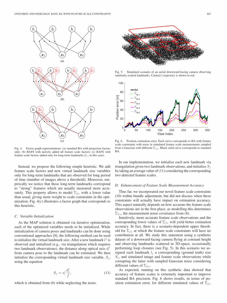
Fig. 4. Factor graph representations: (a) standard BA with projection factorsonly; (b) BAFS with naıvely added all feature scale factors; (c) BAFS withfeature scale factors added only for long-term landmarks (l1 , in this case).

Instead, we propose the following simple heuristic. We addfeature scale factors and new virtual landmark size variablesonly for long-term landmarks that are observed for long periodof time (number of images above a threshold). Moreover, em-pirically we notice that these long-term landmarks correspondto ”strong” features which are usually measured more accu-rately. This property allows to model Σf s with a lower valuethan usual, giving more weight to scale constraints in the opti-mization. Fig. 4(c) illustrates a factor graph that corresponds tothis heuristic.

C. Variable Initialization

As the MAP solution is obtained via iterative optimization,each of the optimized variables needs to be initialized. Whileinitialization of camera poses and landmarks can be done usingconventional approaches [9], the following method can be usedto initialize the virtual landmark size. After a new landmark lj isobserved and initialized (e.g., via triangulation which requirestwo landmark observations), the distance along optical axis dJ

i

from camera pose to the landmark can be estimated. We theninitialize the corresponding virtual landmark size variable, Sj ,using the equation

Sj = sji

dji

f, (11)

which is obtained from (6) while neglecting the noise.

Fig. 5. Simulated scenario of an aerial downward-facing camera observingrandomly-scatted landmarks. Camera’s trajectory is shown in red.

Fig. 6. Position estimation error. Each curve corresponds to BA with featurescale constraints with noise in simulated feature scale measurements sampledfrom a Gaussian with different Σf s . Black solid curve corresponds to standardBA.

In our implementation, we initialize each new landmark viatriangulation given two landmark observations, and initialize Sj

by taking an average value of (11) considering the correspondingtwo detected feature scales.

D. Enhancement of Feature Scale Measurement Accuracy

Thus far, we incorporated our novel feature scale constraints(10) within bundle adjustment, but did not discuss when theseconstraints will actually have impact on estimation accuracy.This aspect naturally depends on how accurate the feature scaleobservations are in the first place, as modelling this determinesΣf s , the measurement noise covariance from (8).

Intuitively, more accurate feature scale observations and thecorresponding lower values of Σf s will yield better estimationaccuracy. In fact, there is a scenario-dependent upper thresh-old for Σf s at which the feature scale constraints will have nocontribution at all. We study this statement using a syntheticdataset of a downward-facing camera flying at constant heightand observing landmarks scattered in 3D-space, occasionallyperforming loop closures (see Fig. 5). In this scenario we as-signed each landmark lj a corresponding (ground truth) sizeSj , and simulated image and feature scale observations whilecorrupting the latter with sampled Gaussian noise consideringdifferent values of Σf s .

As expected, running on this synthetic data showed thataccuracy of feature scales is extremely important to improvestandard BA precision. Fig. 6 shows results, in terms of po-sition estimation error, for different simulated values of Σf s


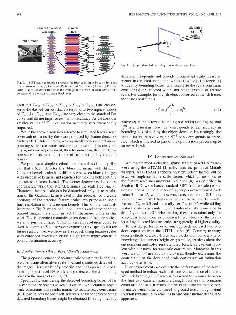
Fig. 7. SIFT scale estimation process. (a) Blur each input image with a setof Gaussian kernels. (b) Calculate Difference of Gaussians (DoG). (c) Featurescale is set via interpolation or as the average of the two Gaussian kernels thatcorrespond to the local-maxima DoG layer.

such that Σf s1 > Σf s2 > Σf s3 > Σf s4 > Σf s5 . One can ob-serve the dashed curves, that correspond to two highest valuesof Σf s (i.e., Σf s1 and Σf s2) are very close to the standard BAcurve, and do not improve estimation accuracy. As we considersmaller values of Σf s , estimation accuracy gets dramaticallyimproved.

While the above discussion referred to simulated feature scaleobservations, in reality these are produced by feature detectorssuch as SIFT. Unfortunately, we empirically observed that incor-porating scale constraints into the optimization does not yieldany significant improvement, thereby indicating the actual fea-ture scale measurements are not of sufficient quality (i.e., toonoisy).

We propose a simple method to address this difficulty. Re-call that a SIFT detector first blurs the image with differentGaussian kernels, calculates difference between blurred imageswith successive kernels, and searches for maxima both spatiallyand across different kernels. The former determines the featurecoordinates, while the latter determines the scale (see Fig. 7).Therefore, feature scale can be determined only up to resolu-tion of the Gaussian kernels used in this process. To increaseaccuracy of the detected feature scales, we propose to use afiner resolution of the Gaussian kernels. This simple idea is il-lustrated in Fig. 7, where additional kernels and correspondingblurred images are shown in red. Furthermore, while in thiswork Σf s is specified manually given detected feature scales,we envision the utilized Gaussian kernels resolution could beused to determine Σf s . However, exploring this aspect is left forfuture research. As we show in the sequel, using feature scaleswith enhanced resolution yields a significant improvement inposition estimation accuracy.

E. Application to Object-Based Bundle Adjustment

The proposed concept of feature scale constraints is applica-ble also using alternative scale invariant quantities detected inthe images. Here, we briefly describe one such application, con-sidering object-level BA while using detected object boundingboxes in the images (see Fig. 8).

Specifically, considering the detected bounding boxes of faraway stationary objects as scale invariant, we formulate objectscale constraints in a similar manner to feature scale constraints(6). Close objects are not taken into account as the correspondingdetected bounding boxes might be obtained from significantly

Fig. 8. Object detected bounding box in the image plane.

different viewpoints and provide inconsistent scale measure-ments. In our implementation, we use HoG object detector [1]to identify bounding boxes, and formulate the scale constraintconsidering the detected width and height instead of featurescale. For example, for the jth object observed at the ith frame,the scale constraint is

wji = f

Sobjj

dji

+ vobji , (12)

where wji is the detected bounding box width (see Fig. 8), and

vobji is a Gaussian noise that corresponds to the accuracy in

bounding box picked by the object detector. Interestingly, thevirtual landmark size variable Sobj

j now corresponds to objectsize, which is inferred as part of the optimization process, up toan overall scale.

IV. EXPERIMENTAL RESULTS

We implemented a classical sparse feature based BA frame-work using the GTSAM [2] solver and the provided Matlabwrapper. As GTSAM supports only projection factors out ofbox, we implemented a scale factor, which corresponds tothe feature scale measurement likelihood (8). As described inSection III-D, we enhance standard SIFT feature scale resolu-tion by increasing the number of layers per octave from defaultvalue 3 up to 15, which, however, consumed about 2.5 timesmore runtime of SIFT feature extraction. In the reported resultswe used Σv = 0.5 and manually set Σf s to 0.2 while addingfeature scale constraints for all landmarks. We were able todrop Σf s down to 0.1 when adding these constraints only forlong-term landmarks, as empirically we observed the corre-sponding detected feature scales are typically of higher quality.

To test the performance of our approach we used two out-door sequences from the KITTI dataset [6]. Contrary to manyother methods tested on this dataset, we do not involve any priorknowledge like camera height or typical object sizes about theenvironment and solve pure standard bundle adjustment prob-lem with our novel feature scale constraints. Moreover, in thiswork we do not use any loop closures, thereby examining thecontribution of the developed scale constraints on estimationaccuracy over time.

In our experiments we evaluate the performance of the devel-oped method to reduce scale drift across a sequence of frames.We initialize the global scale with ground truth range betweenthe first two camera frames, although odometry informationcould also be used. It makes it easy to evaluate estimation per-formance versus time compared to ground truth, though actualsolution remains up to scale, as in any other monocular SLAMapproach.


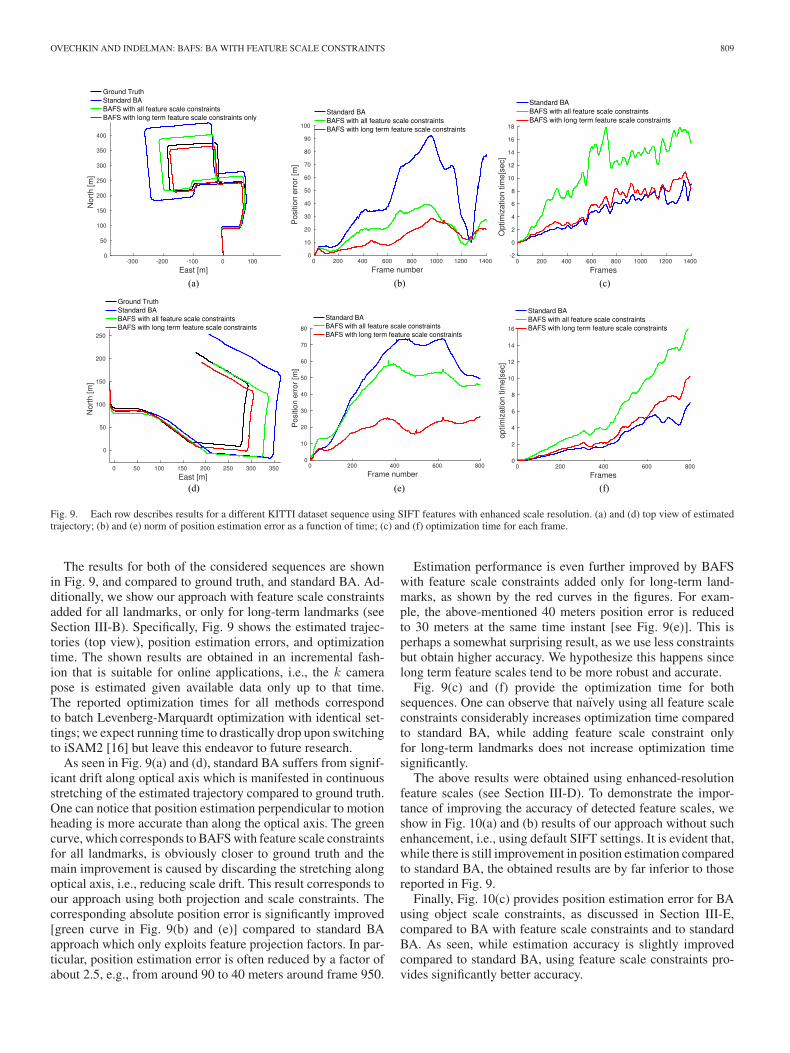
Fig. 9. Each row describes results for a different KITTI dataset sequence using SIFT features with enhanced scale resolution. (a) and (d) top view of estimatedtrajectory; (b) and (e) norm of position estimation error as a function of time; (c) and (f) optimization time for each frame.

The results for both of the considered sequences are shownin Fig. 9, and compared to ground truth, and standard BA. Ad-ditionally, we show our approach with feature scale constraintsadded for all landmarks, or only for long-term landmarks (seeSection III-B). Specifically, Fig. 9 shows the estimated trajec-tories (top view), position estimation errors, and optimizationtime. The shown results are obtained in an incremental fash-ion that is suitable for online applications, i.e., the k camerapose is estimated given available data only up to that time.The reported optimization times for all methods correspondto batch Levenberg-Marquardt optimization with identical set-tings; we expect running time to drastically drop upon switchingto iSAM2 [16] but leave this endeavor to future research.

As seen in Fig. 9(a) and (d), standard BA suffers from signif-icant drift along optical axis which is manifested in continuousstretching of the estimated trajectory compared to ground truth.One can notice that position estimation perpendicular to motionheading is more accurate than along the optical axis. The greencurve, which corresponds to BAFS with feature scale constraintsfor all landmarks, is obviously closer to ground truth and themain improvement is caused by discarding the stretching alongoptical axis, i.e., reducing scale drift. This result corresponds toour approach using both projection and scale constraints. Thecorresponding absolute position error is significantly improved[green curve in Fig. 9(b) and (e)] compared to standard BAapproach which only exploits feature projection factors. In par-ticular, position estimation error is often reduced by a factor ofabout 2.5, e.g., from around 90 to 40 meters around frame 950.

Estimation performance is even further improved by BAFSwith feature scale constraints added only for long-term land-marks, as shown by the red curves in the figures. For exam-ple, the above-mentioned 40 meters position error is reducedto 30 meters at the same time instant [see Fig. 9(e)]. This isperhaps a somewhat surprising result, as we use less constraintsbut obtain higher accuracy. We hypothesize this happens sincelong term feature scales tend to be more robust and accurate.

Fig. 9(c) and (f) provide the optimization time for bothsequences. One can observe that naıvely using all feature scaleconstraints considerably increases optimization time comparedto standard BA, while adding feature scale constraint onlyfor long-term landmarks does not increase optimization timesignificantly.

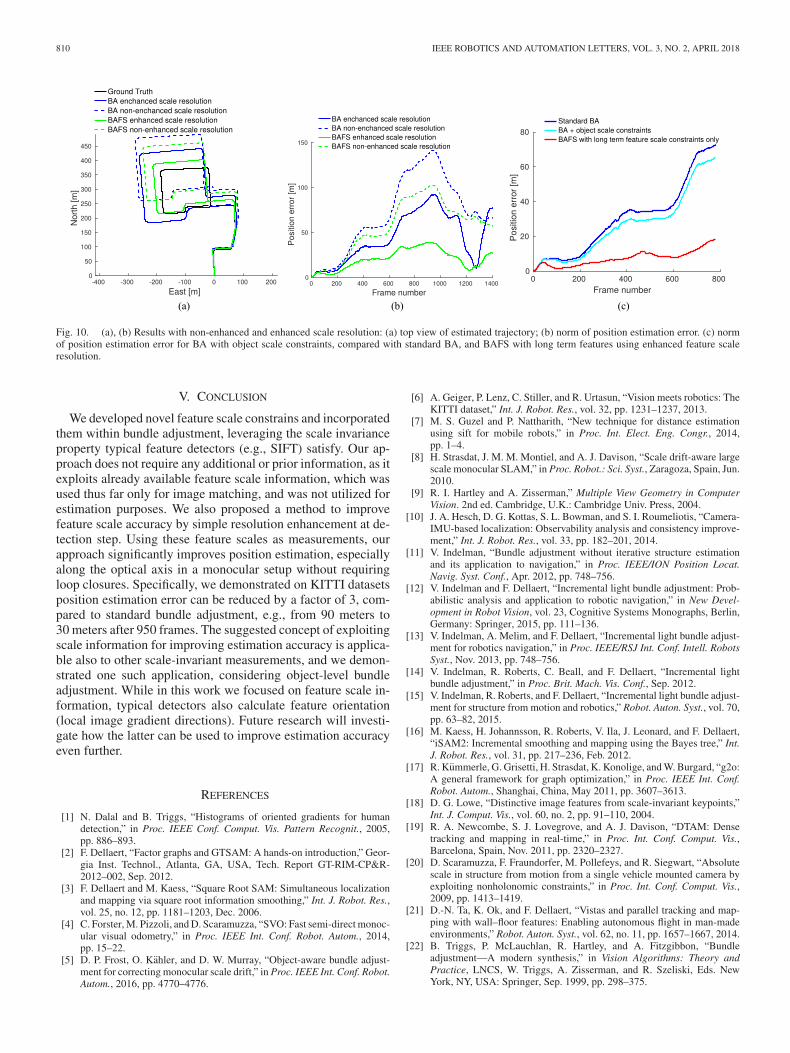
The above results were obtained using enhanced-resolutionfeature scales (see Section III-D). To demonstrate the impor-tance of improving the accuracy of detected feature scales, weshow in Fig. 10(a) and (b) results of our approach without suchenhancement, i.e., using default SIFT settings. It is evident that,while there is still improvement in position estimation comparedto standard BA, the obtained results are by far inferior to thosereported in Fig. 9.

Finally, Fig. 10(c) provides position estimation error for BAusing object scale constraints, as discussed in Section III-E,compared to BA with feature scale constraints and to standardBA. As seen, while estimation accuracy is slightly improvedcompared to standard BA, using feature scale constraints pro-vides significantly better accuracy.


Fig. 10. (a), (b) Results with non-enhanced and enhanced scale resolution: (a) top view of estimated trajectory; (b) norm of position estimation error. (c) normof position estimation error for BA with object scale constraints, compared with standard BA, and BAFS with long term features using enhanced feature scaleresolution.

V. CONCLUSION

We developed novel feature scale constrains and incorporatedthem within bundle adjustment, leveraging the scale invarianceproperty typical feature detectors (e.g., SIFT) satisfy. Our ap-proach does not require any additional or prior information, as itexploits already available feature scale information, which wasused thus far only for image matching, and was not utilized forestimation purposes. We also proposed a method to improvefeature scale accuracy by simple resolution enhancement at de-tection step. Using these feature scales as measurements, ourapproach significantly improves position estimation, especiallyalong the optical axis in a monocular setup without requiringloop closures. Specifically, we demonstrated on KITTI datasetsposition estimation error can be reduced by a factor of 3, com-pared to standard bundle adjustment, e.g., from 90 meters to30 meters after 950 frames. The suggested concept of exploitingscale information for improving estimation accuracy is applica-ble also to other scale-invariant measurements, and we demon-strated one such application, considering object-level bundleadjustment. While in this work we focused on feature scale in-formation, typical detectors also calculate feature orientation(local image gradient directions). Future research will investi-gate how the latter can be used to improve estimation accuracyeven further.

REFERENCES

[1] N. Dalal and B. Triggs, “Histograms of oriented gradients for humandetection,” in Proc. IEEE Conf. Comput. Vis. Pattern Recognit., 2005,pp. 886–893.

[2] F. Dellaert, “Factor graphs and GTSAM: A hands-on introduction,” Geor-gia Inst. Technol., Atlanta, GA, USA, Tech. Report GT-RIM-CP&R-2012–002, Sep. 2012.

[3] F. Dellaert and M. Kaess, “Square Root SAM: Simultaneous localizationand mapping via square root information smoothing,” Int. J. Robot. Res.,vol. 25, no. 12, pp. 1181–1203, Dec. 2006.

[4] C. Forster, M. Pizzoli, and D. Scaramuzza, “SVO: Fast semi-direct monoc-ular visual odometry,” in Proc. IEEE Int. Conf. Robot. Autom., 2014,pp. 15–22.

[5] D. P. Frost, O. Kahler, and D. W. Murray, “Object-aware bundle adjust-ment for correcting monocular scale drift,” in Proc. IEEE Int. Conf. Robot.Autom., 2016, pp. 4770–4776.

[6] A. Geiger, P. Lenz, C. Stiller, and R. Urtasun, “Vision meets robotics: TheKITTI dataset,” Int. J. Robot. Res., vol. 32, pp. 1231–1237, 2013.

[7] M. S. Guzel and P. Nattharith, “New technique for distance estimationusing sift for mobile robots,” in Proc. Int. Elect. Eng. Congr., 2014,pp. 1–4.

[8] H. Strasdat, J. M. M. Montiel, and A. J. Davison, “Scale drift-aware largescale monocular SLAM,” in Proc. Robot.: Sci. Syst., Zaragoza, Spain, Jun.2010.

[9] R. I. Hartley and A. Zisserman,” Multiple View Geometry in ComputerVision. 2nd ed. Cambridge, U.K.: Cambridge Univ. Press, 2004.

[10] J. A. Hesch, D. G. Kottas, S. L. Bowman, and S. I. Roumeliotis, “Camera-IMU-based localization: Observability analysis and consistency improve-ment,” Int. J. Robot. Res., vol. 33, pp. 182–201, 2014.

[11] V. Indelman, “Bundle adjustment without iterative structure estimationand its application to navigation,” in Proc. IEEE/ION Position Locat.Navig. Syst. Conf., Apr. 2012, pp. 748–756.

[12] V. Indelman and F. Dellaert, “Incremental light bundle adjustment: Prob-abilistic analysis and application to robotic navigation,” in New Devel-opment in Robot Vision, vol. 23, Cognitive Systems Monographs, Berlin,Germany: Springer, 2015, pp. 111–136.

[13] V. Indelman, A. Melim, and F. Dellaert, “Incremental light bundle adjust-ment for robotics navigation,” in Proc. IEEE/RSJ Int. Conf. Intell. RobotsSyst., Nov. 2013, pp. 748–756.

[14] V. Indelman, R. Roberts, C. Beall, and F. Dellaert, “Incremental lightbundle adjustment,” in Proc. Brit. Mach. Vis. Conf., Sep. 2012.

[15] V. Indelman, R. Roberts, and F. Dellaert, “Incremental light bundle adjust-ment for structure from motion and robotics,” Robot. Auton. Syst., vol. 70,pp. 63–82, 2015.

[16] M. Kaess, H. Johannsson, R. Roberts, V. Ila, J. Leonard, and F. Dellaert,“iSAM2: Incremental smoothing and mapping using the Bayes tree,” Int.J. Robot. Res., vol. 31, pp. 217–236, Feb. 2012.

[17] R. Kummerle, G. Grisetti, H. Strasdat, K. Konolige, and W. Burgard, “g2o:A general framework for graph optimization,” in Proc. IEEE Int. Conf.Robot. Autom., Shanghai, China, May 2011, pp. 3607–3613.

[18] D. G. Lowe, “Distinctive image features from scale-invariant keypoints,”Int. J. Comput. Vis., vol. 60, no. 2, pp. 91–110, 2004.

[19] R. A. Newcombe, S. J. Lovegrove, and A. J. Davison, “DTAM: Densetracking and mapping in real-time,” in Proc. Int. Conf. Comput. Vis.,Barcelona, Spain, Nov. 2011, pp. 2320–2327.

[20] D. Scaramuzza, F. Fraundorfer, M. Pollefeys, and R. Siegwart, “Absolutescale in structure from motion from a single vehicle mounted camera byexploiting nonholonomic constraints,” in Proc. Int. Conf. Comput. Vis.,2009, pp. 1413–1419.

[21] D.-N. Ta, K. Ok, and F. Dellaert, “Vistas and parallel tracking and map-ping with wall–floor features: Enabling autonomous flight in man-madeenvironments,” Robot. Auton. Syst., vol. 62, no. 11, pp. 1657–1667, 2014.

[22] B. Triggs, P. McLauchlan, R. Hartley, and A. Fitzgibbon, “Bundleadjustment—A modern synthesis,” in Vision Algorithms: Theory andPractice, LNCS, W. Triggs, A. Zisserman, and R. Szeliski, Eds. NewYork, NY, USA: Springer, Sep. 1999, pp. 298–375.

BAFS: Bundle Adjustment With Feature Scale Constraints for ...

Documents

Transcript of BAFS: Bundle Adjustment With Feature Scale Constraints for ...