Annals of Biomedical Engineering, Vol. 23, pp. 116-126, 1995 0090-6964/95 $10.50 + .00 Printed in the USA. All rights reserved. Copyright �9 1995 Biomedical Engineering Society

Magnetic Stimulation of Axons in a Nerve Bundle: Effects of Current Redistribution in the Bundle

SRIKANTAN S. NAGARAJAN, '~ DOMINIQUE M . D U R A N D , t BRADLEY J. ROTH,:~ a n d

RANJITH S . WIJESINGHEw

1Applied Neural Control Laboratory, Department of Biomedical Engineering, Case Western Reserve University, Cleveland, OH; SBiomedical Engineering and Instrumentation Program, National Center for Research Resources, National Institutes of Health,

Bethesda, MD; and w of Biomedical Engineering, Tulane University, New Orleans, LA

AbstractmRecently, we developed a model of magnetic stimu- lation of a concentric axon in an anisotropic nerve bundle. In that earlier paper, we considered a single axon surrounded by a nerve bundle represented as a homogeneous anisotropic monodomain medium. In this paper we extend our previous calculations to examine excitation of axons within a nerve bundle without ne- glecting the presence of other axons in the nerve bundle. A three-dimensional axial symmetry volume conductor model is used to determine the transmembrane potential response along an axon due to induced electric fields produced by a toroidal coil. Our principal objective is to examine the effect of current redis- tribution to other axons in the bundle on excitation characteris- tics. We derive the transmembrane potential along an axon for two currently available models of current redistribution: the biodomain model and the spatial-frequency monodomain model. Results indicate that a reduction in the transmembrane potential along an axon due to the presence of other nerve fibers in the bundle is observed. Axons located at the periphery of a nerve bundle have lower thresholds and different excitation sites com- pared with axons located near the center of a nerve bundle.

Keywords--Magnetic Stimulation, Electrical stimulation, An- isotropy, Coils, Transmembrane response, Nerve Bundle, Perineurium, Sheath, Bidomain, Spatial-frequency conductiv- ity, Monodomain, Cable Equation, Volume conductor effects.

INTRODUCTION

Magnetic stimulation is a noninvasive technique used to activate the nervous system and has emerged in recent years as a useful diagnostic and clinical tool (6). Despite its usefulness, many of the basic mechanisms of excitation of nerves during magnetic stimulation are not year clear. Quantitative and complex models of magnetic stimulation

Acknowledgment--This work was supported in part by National Sci- ence Foundation grant BCS91-11503 and National Institutes of Health grant 1R01NS32572-01A1 to Dominique M. Durand.

Address correspondence to Dominique M. Durand, Applied Neural Control Laboratory, Department of Biomedical Engineering, Case West- em Reserve University, Cleveland, OH 44106-4912.

(Received 30ct94, Revised lOJan95, Accepted 13Jan95)

have proven useful in understanding some of the basic mechanisms of excitation (4,5,11,12,16,21), and predic- tions based on such models have been verified experimen- tally (15,19). Most existing models assume that the target axon is isolated and lying in a homogeneous, isotropic volume conductor. A nerve, however, contains many ax- ons held together in a bundle. The properties of excitation of axons depend not only on the properties of the axons themselves, but also on the properties of the bundle, such as how tightly the axons are packed, and the anisotropic

conductivity of the nerve tissue. Recently, we have developed a model of a concentric

axon located in a uniform anisotropic nerve bundle (18). In that model we determined that nerve bundle anisotropy and the presence of a perineurium can significantly affect the amplitude of transmembrane polarization and the lo- cation of excitation along an axon. However, in the earlier paper (18), we had chosen to neglect the effect of the other axons within the nerve bundle. More appropriate repre- sentations of neural tissue, however, are either a bidomain medium consisting of a coupled interstitial and intracellu- lar spaces or a monodomain medium in which the bundle conductivity depends on spatial frequency (22,23). In this

paper we extend our previous calculations to examine ex- citation characteristics of axons within a nerve bundle modeled as a bidomain medium and a monodomain me- dium with a spatial f requency-dependent conductivity. Our aim is to examine (a) the effect of current redistribu- tion within a nerve bundle on excitation characteristics, (b) the effect of the perineurium using more complex rep- resentations of the nerve bundle such as the bidomain and spatial-frequency monodomain models, and (c) the trans- membrane polarization of axons located at different radial positions within the nerve. In all of these models, we assume that the nerve bundle is surrounded by a perineu- rium and a three-dimensional axisymmetric volume con- ductor.

116

Magnetic Stimulation of Axons in a Nerve Bundle 117

THEORY

Applied Fields

The total electric field in a volume conductor can be expressed as the sum of an induced term and an electro- static term. The induced term Einduce d is due to the applied time-varying magnetic field, and the electrostatic term (Eohmic) arises from charge separation at the boundaries of the volume conductor. Therefore the total electric field is

Etota I = Einduce d + Eohmi c (1)

We assume that the induced component of electric field is created by a thin toroidal coil (5,16). This geometry has been used recently by Davey et al. to stimulate nerves in vitro (10). Similar to previously published calculations, we also assume that the toroidal coil creates a thin filament of time-varying magnetic flux ~ of radius c. Therefore, the magnetic field has only an azimuthal component and can be written in cylindrical coordinates using dirac-delta functions as shown in the following equations:

Bapplie d = ~ t ~ ( p - C)~(Z) (2)

where ff is the unit vector in the azimuthal direction. The induced electric field is calculated from the vector poten- tial by

aA Einduced = -- 0"--t- (3)

where the vector potential is calculated using the equations

and

V . A = 0

V • A = B (4)

We can express the time rate of change of the vector potential (A) as a function of k, the Fourier transformed variable of the axial variable z as (5,9,14)

dO(t) ik6(Iklp)g~(Iklc), p < c (5) A~ = - c

dO(t) �9 ~z(t,p,k) = - c T IklIo(Iklo)gl(Iklc), p < c (6)

where I o, 11, Ko, and K 1 are modified Bessel functions of the zeroth and first-order, and t represents time.

The electrostatic component of the electric field ac- counts for the contribution to the electric field arising from charge accumulation at boundaries of the volume conduc- tor and can be expressed as follows

Eohmi c = -- Vdxb (7)

In the subsequent sections, we determine the scalar poten- tials and thereby the electrostatic component of the electric

field for the different volume conductor models of an axon in a nerve bundle.

Isolated Axon Located in an Infinite Homogeneous Conducting Medium

In the case of an axon located in an infinite homoge- neous conducting medium, space is divided into three re- gions, intracellular (i), extracellular (e), and membrane (m). The scalar potential in each regions dPi, d~m, dPe sat- isfies Laplace's equation,

V2(I)i,m,e = 0 (8 )

Owing to azimuthal symmetry, expanding this equation in cylindrical coordinates we get

1 0 ( 0(I)i,m,e~ OZ2(I)i m e p Op p ---~p /I + Oz------~:- - 0 (9)

Equation 9 reduces to a modified Bessel's equations when applying a Fourier transform to the axial variable z as shown below:

1 d ( ddPi,m,e'~_ k2dPim e -= 0 ( 1 0 ) p dp _ p dp ] ' '

Solutions to these equations can be expressed using mod- ified Bessel functions

~i(t,p,k) = A(t,k)lo(lklp), p < ai

~ m ( t , p , k ) = n(t,k)lo(lklp) + C(t,k)go(Jklp), a i < p < ao

a~e(t,p,k) -- D(t,k)go([klp), p > ao (11)

The coefficients A, B, C, and D can be determined by applying the appropriate boundary conditions (see Appen- dix). We are interested in solving for the transmembrane potential, which is defined as the difference between the intracellular and extracellular potentials:

~Igtm(t,k ) = dPm(t, ai,k ) - dPm(t, ao,k ) ( 1 2 )

Basser et al. (5) have derived a similar analytical expres- sion for transmembrane potential as a function of k by approximating the membrane as a thin dipole surface of thickness d (Eq. 12 from Ref. 5), which results in identical solutions (16).

Axon in an Anisotropic Monodomain Nerve Bundle

We now consider an axon within a bundle, which is anisotropic with a conductivity different from that of the extracellular space (7,9,17). The interstitial medium is then assumed to be surrounded by a perineurium. Three- dimensional space is divided into five regions: intracellu- lar (i), membrane (m), bundle/interstitial (b), sheath (s), and extracellular (e). All of the regions except the bundle are assumed to be isotropic and satisfy the modified ho-

118 S . S . NAGARAJAN et al.

mogeneous Bessel's equations, whose solutions reduce to the following equations:

qbi(t,p,k) = A(t,k)lo(lklp), p < ai

qbm(t,p,k) = B(t,k)lo(lklp) + C(t,k)Ko(lklp), ai < p < ao

~s(t,p,k) = F(t,k)1o(lklp) + G(t,k)Ko(lklP), bi < p < bo

qbe(t,p,k) = H(t,k)Ko(Iklp), p > bo (13)

where the unknown coefficients A, B, C, F, G, and H are determined from the boundary conditions. In an anisotro- pic region, such as the nerve bundle, the potentials satisfy

V " [~b( - - /~b -- V(IDb) ] = 0 (14)

where ~b is the conductivity tensor. We assume that the conductivity in the bundle is constant but is different in the radial and axial direction. The axial component of the bundle conductivity is related linearly to the conductivities in these regions through the volume fraction

o-~ = o ' i f + O" e (1 --3 ' ) (15)

The eight unknown coefficients, A-H, are determined by the boundary conditions (see Appendix).

Axons in a Bidomain Nerve Bundle

In the previous model we neglected the effect of current redistribution due to the presence of other fibers in the nerve bundle. The "bidomain concept" accounts for the presence of multiple fibers (1,20). This is a continuum model that accounts for both the intracellular and the in- terstitial spaces. The tissue is described by five parame- ters: the intracellular axial conductivity, o-iz; the interstitial

o and o. the membrane axial and radial conductivities, o-z o-0, resistance per unit area, Rm; and the ratio of the membrane surface area to the tissue volume, 13. Current in the bido- main is governed by two equations for the intracellular and the interstitial regions

V �9 Ji = - l m (20)

V "Jo = ]m (21)

where I m is the membrane current per unit volume. For a passive linear membrane, we can express I m as

where f is the fraction of volume occupied by the intra- cellular space. When we define the anisotropy ratio within the bundle as

(16)

the potential in the bundle satisfies the inhomogeneous modified Bessel's equation:

13 Im = R m ( ~ i - qbo) (22)

where 13 is the ratio of membrane surface to tissue volume (18) and R m the membrane resistance per unit area (20). We assume that the bidomain conductivities are related to the volume fraction by

o z = f ~

1 d ( dq~b'~ _ hbekZq~b = --(1 -- hbZ)ikkz (17) oN P do/

where i is the imaginary number. The solution to Eq. 17 is the sum of a general solution to the homogeneous equation and a particular solution to the inhomogeneous equation:

�9 b(t,p,k) -- O(t,k)lo(IklXp) + E(t,k)go(lklXp)

+ ~(t,k)Io(lk[p), a0 < p < bi (18)

where D and E must also be determined from the boundary conditions. The third term of Eq. 18 is the particular so- lution to the inhomogeneous modified Bessel's Eq. 17, where

~(t,k) dO ik

-- - c 7 ; ~1 gm(Iklc) Xb # 1

= 0 , hb = 1

(19)

l - f o-~ 1 + f o - e

o-~ = (1 - J)o-e (23)

The current densities are related to the potentials through Ohm's law:

Ji = ~ i ( - A i - V(I)i) (24)

Jo = ~ o ( - A o - V ~ o ) (25)

where Fi and Fo are the conductivity tensors

~i = 0 (26)

0 o-i

Magnetic Stimulation of Axons in a Nerve Bundle 119

and 4Po = A(k)lo(Ikl'qhp) + ~(k)Zo(lklp) (32)

[~o ~ o o) ~~ ~00 ~176176 O0 o" o (27)

Since the nerve axons making up the bundle are not cou- pled by intracellular junctions in the radial direction, the intracellular radial conductivity in the bidomain model vanishes (22). Substituting Eqs. 26, 24, and 22 in Eq. 20 and expanding the divergence operator in cylindrical co- ordinates, we can obtain an algebraic expression for the intracellular potentials by taking the Fourier transform of the axial variable z as shown below:

1 i k ~ m ~

- qbo(t, p,k) Zm ~i(t, p,k) Zm o.Zk 2 + 1 - - o'Zk 2 + 1

13 13

s

(28)

This equation is analogous to the result for point source electrical stimulation as derived by Altman and Plonsey (1), except for the presence of the second term on the right-hand side. Similarly, substituting Eqs. 27, 25, and 22 in Eq. 21, we find that the interstitial potential satisfies the following inhomogeneous modified Bessel's equation:

ld( a% P dP P do ] -- Ti2h2k2(I)o = ( z o" i

1 - 1 - ~ - ~ +

z) cr o ikk 2 ~kz

Zm-- o'Zk 2 + 1 13 /

(29)

where

/ 1 ) (Zm z-2 rl(k ) = 1 Zm Zk2 1 I g (rik + 1

(30)

and

(31)

Solution to this equation can be written as the sum of a general solution and a particular solution

where ~(k) is the function defined in Eq. 19. We consider the bidomain bundle to be surrounded by

a perineurium sheath, which in turn is surrounded by an unbounded homogeneous conducting medium. The sheath and the extracellular medium are assumed to be isotropic. The potentials in those regions satisfy Laplace's equation, which reduces to a modified Bessel's equation, the solu- tion to which can be expressed as

�9 s(t,o,k) = n(t,k)to(Iklp) + C(t,k)go(Iklp), bi < p < bo

dPe(t,p,k) = O(t,k)go(Iklp), p > bo (33)

The four unknown coefficients A - D can be determined from the boundary conditions (see Appendix): (a) conti- nuity of the normal component of the current density and (b) the continuity of the tangential component of the elec- tric field at the bidomain-perineurium surface (p = bi) and the perineurium-extracellular interface (p = bo). The current density in the bidomain is the sum of the current densities in the intracellular and interstitial spaces. How- ever, since we assume that the intracellular conductivity in the direction transverse to the fibers is zero, the intracel- lular potentials do not enter these boundary conditions (22).

Axon in a Spatial-Frequency Monodomain Bundle

Another proposed representation of a nerve bundle that takes into account the presence of other nerve fibers is the spatial-frequency monodomain model (23). This model makes use of monodomain conductivities that depend on spatial and temporal frequencies (22,23) and is a general- ization of an earlier description of the electric properties of a bundle of muscle fibers. The macroscopic conductivities % and crp are expressed as functions of the spatial fre- quency k (22):

ere(1 - f ) + cr0e

and

1 - y aW5 ~C(k)- 1 + f ~e + 2R----~- (35)

120 S.S. NAGARAJAN et al.

where R m is the membrane resistance per unit area, and h is the length constant of a single fiber in the restricted interstitial space of the fiber bundle given by

h = (36)

O"

In these equations, o" i and (r e are the intracellular and interstitial conductivity, f is the volume fraction of the intracellular space, and a is the radius of the passive fi- bers. If we assume that an axon is present inside a nerve bundle with these spatial frequency-dependent conductiv- ities, the equations for the anisotropic monodomain can be modified to include the conductivities to be functions of k. In this case, the equations for an anisotropic monodomain model (see Appendix) are now solved by substituting in Eqs. 34, 35, and 36 for the spatial frequency-dependent conductivities and by assuming that the anisotropy ratio is calculated as follows:

Xb(k) = ~/-~b(k) (37)

As in the previous models, the transmembrane potential, as a function of k, of an axon located concentrically in a bundle with spatial frequency~lependent conductivity is determined.

Shift ---~i i"'--

o.~

-10 -5

Filament of flux created by a thin toro~al coi~

- e - Isorated a.~otf . . / -(3 - Sheathless anisotropic monedomain bundle "

z (ram) I 10

-01 ~l

-0,2 " o "

-O 3

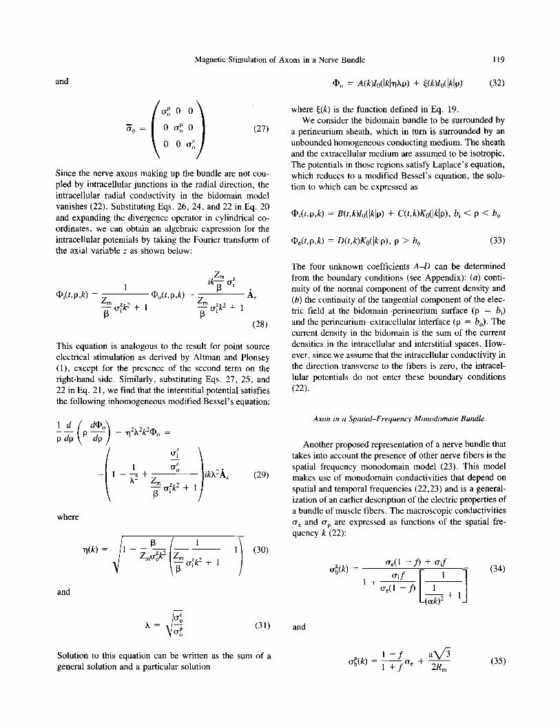
FIGURE 1. Steady-state t ransmembrane potential along an isolated axon (closed circles), an axon located in a sheathless anisotropic nerve bundle (open circles), an axon located in a sheatbless bidomain bundle (closed triangles), and an axon located in a sheathless spatial - frequency monodomain bun- dle (open triangles). The fol lowing parameters were used: b. = 1 mm, cq = 1.4286 S/m, cre = 0.8 S/m, f = 0.7, crm = 62.5 nS/m, arm = 6 nm, ch~/dt = 0.1 T/s, c = 2 m m (chosen from Refs. 1,5,13,17).

i - 1 0 - 5

- 0 . 1

�9 . . o * Sheathless aniso~opic rnonodomain bundle Anisof~pir rnonodomain bundle+pedneunurn

0 .2 - I - .o- Sheathle~ bidornan bundle B / - e - Bidomain bundle*pedne~ium

0 . 1 ~

-0.2 0 . 2 -

C

- 1 0 - 5

- 0 . 1 -

- 0 . 2 -

- .o- Sheath~,s spa~al-frequency rnonodoman bundle - e - Spa~al4reqcency monodomain I~ndle+pe~neufitrn

~ 0

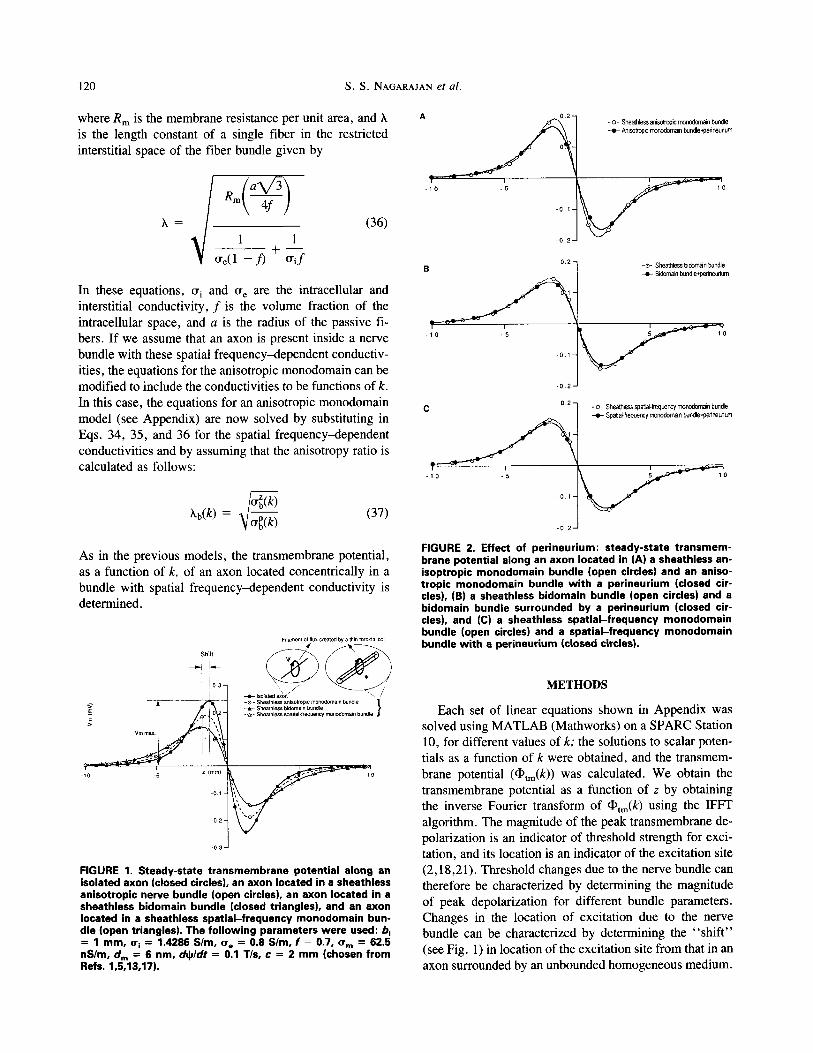
FIGURE 2. Effect of perineurium: steady-state t ransmem- brane potential along an axon located in (A) a sheathless an- isoptropic monodomain bundle (open circles) and an aniso- tropic monodomain bundle wi th a perineurium (closed cir- cles), (B) a sheathless bidomain bundle (open circles) and a bidomain bundle surrounded by a perineurium (closed cir- cles), and (C) a sheathless spat ia l - f requency monodomain bundle (open circles) and a spatial - frequency monodomain bundle wi th a perineurium (closed circlesl.

METHODS

Each set of linear equations shown in Appendix was solved using MATLAB (Mathworks) on a SPARC Station 10, for different values of k; the solutions to scalar poten- tials as a function of k were obtained, and the transmem- brane potential ((I)tm(k)) was calculated. We obtain the transmembrane potential as a function of z by obtaining the inverse Fourier transform of (I)tm(k) using the IFFT algorithm. The magnitude of the peak transmembrane de- polarization is an indicator of threshold strength for exci- tation, and its location is an indicator of the excitation site (2,18,21). Threshold changes due to the nerve bundle can therefore be characterized by determining the magnitude of peak depolarization for different bundle parameters. Changes in the location of excitation due to the nerve bundle can be characterized by determining the "shif t" (see Fig. 1) in location of the excitation site from that in an axon surrounded by an unbounded homogeneous medium.

Magnetic Stimulation of Axons in a Nerve Bundle 121

0.25 A

0.20

0.15

E E 0.10

t r I I

0.05 ..-O- Sheathless anisotropic monodomain --13- Sheathless spatial-frequency monodomain - & - Sheathless bidomain

0.00 I I I I 0.0 0.2 0.4 0.6 0.8

Volume fraction

1.0

B 0.25

0.20

> E o.15

E

E 0 . 1 0 >

0.05

0.00 0.0

I I I |

_ -O- Anisotropic monodomain+perineurium �9 --s Spatial-frequency monodomain+perineurium -~-- Bidomain+perineurium

I I I I 0.2 0.4 0.6 0.8 1.0

Volume fraction

C 0.0

g = - 0 . 5 o

m o "~ -1.0 ID

.c _ 1 . 5 =_ ~ = s o t or pic monodomain ~, '- ~ a l - f r e q u e n c y om nodomair~ O9

-zY.- Sheathless bidomain

-2.0 1 I I I 0 .0 0 . 2 0 . 4 0 . 6 0 . 8 .0

D

E E

c: .o_

N co O CX

.8

.=_ (D

0 . 0 I I I I

-0.5 - O _

- 1 . 0 -

- 1 . 5 -

-4:3-- Spatial-frequency monodomain+peri...~ - & - Bidomain+peri... [ ]

-2.0 I I 1 I 0,0 0.2 0,4 0.6 0.8 1.0

Volume fract ion VoJume fract ion

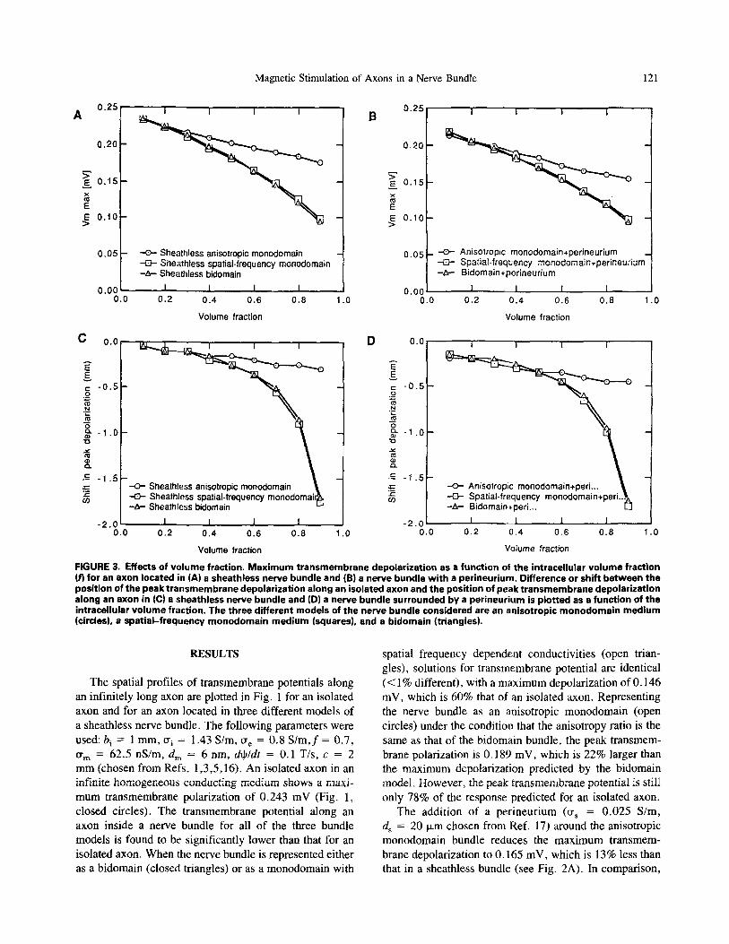
FIGURE 3. Effects of volume fraction. Max imum transmembrane depolarization as a function of the intracellular volume fraction (f) for an axon located in (A) a sheathless nerve bundle and (B) a nerve bundle wi th a perineurium. Difference or shift between the position of the peak t ransmembrane depolarization along an isolated axon and the position of peak t ransmembrane depolarization along an axon in (C) a sheathless nerve bundle and (D) a nerve bundle surrounded by a perineurium is plotted as a function of the intracellular volume fraction. The three different models of the nerve bundle considered are an anisotropic monodomain medium (circles), a spatial - frequency monodomain medium (squares), and a bidomain (triangles).

RESULTS

The spatial profiles of transmembrane potentials along an infinitely long axon are plotted in Fig. 1 for an isolated axon and for an axon located in three different models of a sheathless nerve bundle. The following parameters were

used: b i = 1 mm, tr i = 1.43 S/m, ~ = 0.8 S / m , f = 0.7, tr~ = 62.5 nS/m, d,~ = 6 nm, dO~dr = 0.1 T/s , c = 2

mm (chosen from Refs. 1,3,5,16). An isolated axon in an infinite homogeneous conducting medium shows a maxi- mum transmembrane polarization of 0.243 mV (Fig. 1, closed circles). The transmembrane potential along an axon inside a nerve bundle for all of the three bundle models is found to be significantly lower than that for an isolated axon. When the nerve bundle is represented either as a bidomain (closed triangles) or as a monodomain with

spatial f requency~lependent conductivities (open trian- gles), solutions for transmembrane potential are identical ( < 1% different), with a maximum depolarization of 0.146 mV, which is 60% that of an isolated axon. Representing the nerve bundle as an anisotropic monodomain (open circles) under the condition that the anisotropy ratio is the same as that of the bidomain bundle, the peak transmem- brane polarization is 0.189 mV, which is 22% larger than the maximum depolarization predicted by the bidomain model. However, the peak transmembrane potentiai is still only 78% of the response predicted for an isolated axon.

The addit ion of a per ineurium ( ~ = 0.025 S/m, d s = 20 p~m chosen from Ref. 17) around the anisotropic monodomain bundle reduces the maximum transmem- brahe depolarization to 0.165 mV, which is 13% less than that in a sheathless bundle (see Fig. 2A). In comparison,

1 2 2 S . S . NAGARAJAN et al.

A 0.25

0 .20 -

:~ 0 .15

E E 0 .10 >

0 . 0 5 ,

0 . 0 C 0.0

C 0 . 0

Z g = - 0 . 5 ._o

~ -1.0 " o

-=- - 1 . 5 .=_

�9 - o - Sheathless anisotropic monodomain Sheathless spatial-frequency monodomain

-&-- Sheathless bidomain

I 1 I I 0.2 0.4 0 .6 0.8

Bundle Radius [mini

1.0

�9 - 0 - Sheathless anisotropic monodomain �9 --C- Sheathless spatial-frequency monodomain -Zx- Sheathless bidomain

I I I I 0.2 0 .4 0.6 0.8

B 0.25

D

0.20

>

0.15

E E 0 .10 >

0 .05

0 . 0 0 0 . 0

0 . 0

Z E

v

= - 0 . 5 c)

c0 N "F-

O g -1 .o

"1o

.=- - 1 .5

- 2 . 0 - 2 . 0 0.0 1.0 0.0

_ - O - - Anisotropic monodomain+perineurium �9 -13- Spatial- frequency monodornain+perineuriurn -~ . - Bidomain+perineur ium

I I I 1 0.2 0 .4 0 .6 0 .8

Bundle Radius [ram]

.0

Bundle radius [mini

(9

- 0 - Anisotropic monodomain + perineuriurn -..t3- Spatial-frequency monodomain + perineurium -&..- Bidomain + perineuriurn

I I 1 I 0.2 0 .4 0.6 0 .8 1.0

Bundle radius [mm]

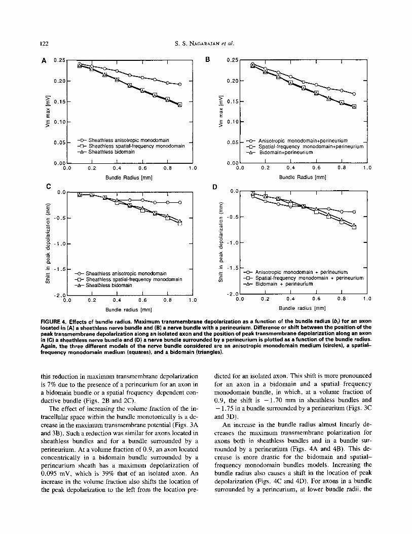
FIGURE 4. Effects of bundle radius. Max imum transmembrane depolarization as a function of the bundle radius (bi) for an axon located in (A) a sheathless nerve bundle and (B) a nerve bundle wi th a perineurium. Difference or shift between the position of the peak t ransmembrane depolarization along an isolated axon and the position of peak t ransmembrane depolarization along an axon in (C) a sheathless nerve bundle and (D) a nerve bundle surrounded by a perineurium is plotted as a function of the bundle radius. Again, the three different models of the nerve bundle considered are an anisotropic monodomain medium (circles), a spatial- frequency monodomain medium (squares), and a bidomain (triangles).

this reduction in maximum transmembrane depolarization is 7% due to the presence of a perineurium for an axon in a bidomain bundle or a spatial frequency~lependent con- ductive bundle (Figs. 2B and 2C).

The effect of increasing the volume fraction of the in- tracellular space within the bundle monotonically is a de- crease in the maximum transmembrane potential (Figs. 3A and 3B). Such a reduction was similar for axons located in sheathless bundles and for a bundle surrounded by a perineurium. At a volume fraction of 0.9, an axon located concentrically in a bidomain bundle surrounded by a perineurium sheath has a maximum depolarization of 0.095 mV, which is 39% that of an isolated axon. An increase in the volume fraction also shifts the location of the peak depolarization to the left from the location pre-

dicted for an isolated axon. This shift is more pronounced for an axon in a bidomain and a spat ia l - f requency monodomain bundle, in which, at a volume fraction of 0.9, the shift is - 1 . 7 0 mm in sheathless bundles and - 1.75 in a bundle surrounded by a perineurium (Figs. 3C and 3D).

An increase in the bundle radius almost linearly de- creases the maximum transmembrane polarization for axons both in sheathless bundles and in a bundle sur- rounded by a perineurium (Figs. 4A and 4B). This de- crease is more drastic for the bidomain and spatial- frequency monodomain bundles models. Increasing the bundle radius also causes a shift in the location of peak depolarization (Figs. 4C and 4D). For axons in a bundle surrounded by a perineurium, at lower bundle radii, the

Magnetic Stimulation of Axons in a Nerve Bundle 123

0 . 3 -

- 1 0 - 5 z (mm

-0.1 -

- 0 . 2 -

0.3

E 0.2 >E

E :~ 0.1

-0 .3

- - vm iso laxon - O - f f ~ = l . 0 - 1 - p/i~ =0,7 " " } " ~ = 0 , 4 -J~V-- p/l~=0.1

I I I I

- C - $heathless bidomain model -c)- BiOomain model with perineurium

~3 13.

0 . 0 I I I I 0.0 0.2 0.4 0.6 0.8 1.0

Axon position from cenler [mm]

0 .8

E" 0.6

.~_ 0,4

.~ 0 .2

o

0 . 2

~- - o . 4

= - 0 , 6 go

- 0 . 8

- c - Sheathless bidomain model �9 -C - Bidomain model with perineurium

0.2 0.4 0.6 0.8

Axon position from center [mm]

1.0

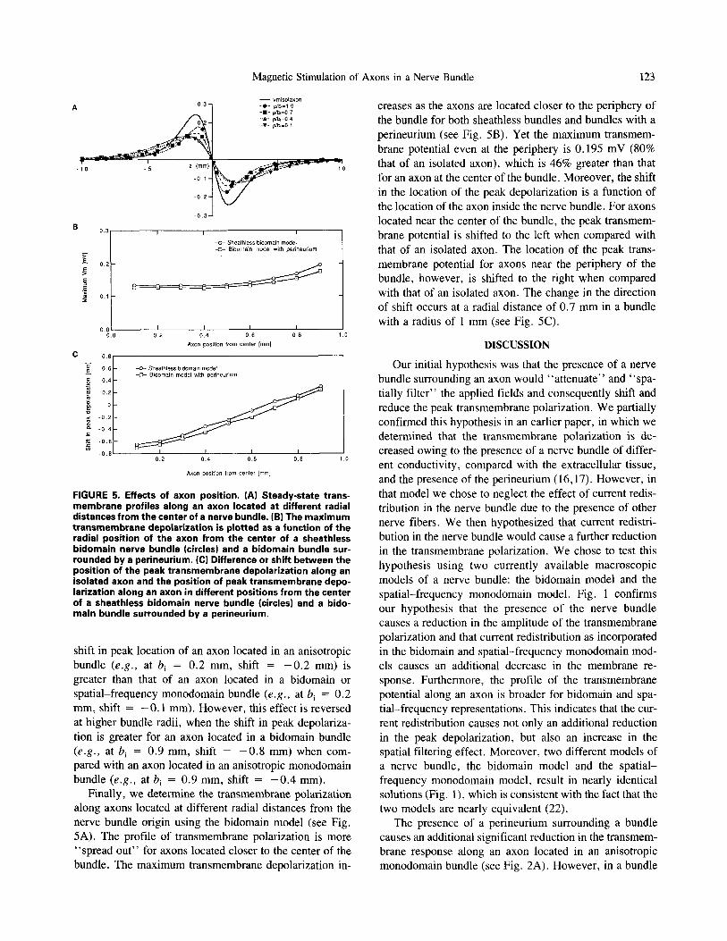
FIGURE 5. Effects of axon position. (A) Steady-state trans- membrane profiles along an axon located at different radial distances from the center of a nerve bundle. (B) The maximum transmembrane depolarization is plotted as a function of the radial position of the axon from the center of a sheathless bidomain nerve bundle (circles) and a bidomain bundle sur- rounded by a perineurium. (C) Difference or shift between the position of the peak transmembrane depolarization along an isolated axon and the position of peak transmembrane depo- larization along an axon in different positions from the center of a sheathless bidomain nerve bundle (circles) and a bido- main bundle surrounded by a perineurium.

shift in peak location of an axon located in an anisotropic bundle (e.g., at b i = 0.2 mm, shift = - 0 . 2 mm) is greater than that of an axon located in a bidomain or spatial-frequency monodomain bundle (e.g., at b i = 0.2 mm, shift = - 0 . 1 mm). However, this effect is reversed at higher bundle radii, when the shift in peak depolariza- tion is greater for an axon located in a bidomain bundle (e.g., at b i = 0.9 mm, shift = - 0 . 8 mm) when com- pared with an axon located in an anisotropic monodomain bundle (e.g., at b i = 0.9 mm, shift = - 0 . 4 mm).

Finally, we determine the transmembrane polarization along axons located at different radial distances from the nerve bundle origin using the bidomain model (see Fig. 5A). The profile of transmembrane polarization is more "spread out" for axons located closer to the center of the bundle. The maximum transmembrane depolarization in-

creases as the axons are located closer to the periphery of the bundle for both sheathless bundles and bundles with a perineurium (see Fig. 5B). Yet the maximum transmem- brane potential even at the periphery is 0.195 mV (80% that of an isolated axon), which is 46% greater than that for an axon at the center of the bundle. Moreover, the shift in the location of the peak depolarization is a function of the location of the axon inside the nerve bundle. For axons located near the center of the bundle, the peak transmem- brane potential is shifted to the left when compared with that of an isolated axon. The location of the peak trans- membrane potential for axons near the periphery of the bundle, however, is shifted to the right when compared with that of an isolated axon. The change in the direction of shift occurs at a radial distance of 0.7 mm in a bundle with a radius of 1 mm (see Fig. 5C).

DISCUSSION

Our initial hypothesis was that the presence of a nerve bundle surrounding an axon would "at tenuate" and "spa- tially filter" the applied fields and consequently shift and reduce the peak transmembrane polarization. We partially confirmed this hypothesis in an earlier paper, in which we determined that the transmembrane polarization is de- creased owing to the presence of a nerve bundle of differ- ent conductivity, compared with the extracellular tissue, and the presence of the perineurium (16,17). However, in that model we chose to neglect the effect of current redis- tribution in the nerve bundle due to the presence of other nerve fibers. We then hypothesized that current redistri- bution in the nerve bundle would cause a further reduction in the transmembrane polarization. We chose to test this hypothesis using two currently available macroscopic models of a nerve bundle: the bidomain model and the spatial-frequency monodomain model. Fig. 1 confirms our hypothesis that the presence of the nerve bundle causes a reduction in the amplitude of the transmembrane polarization and that current redistribution as incorporated in the bidomain and spatial-frequency monodomain mod- els causes an additional decrease in the membrane re- sponse. Furthermore, the profile of the transmembrane potential along an axon is broader for bidomain and spa- tial-frequency representations. This indicates that the cur- rent redistribution causes not only an additional reduction in the peak depolarization, but also an increase in the spatial filtering effect. Moreover, two different models of a nerve bundle, the bidomain model and the spatial- frequency monodomain model, result in nearly identical solutions (Fig. 1), which is consistent with the fact that the two models are nearly equivalent (22).

The presence of a perineurium surrounding a bundle causes an additional significant reduction in the transmem- brane response along an axon located in an anisotropic monodomain bundle (see Fig. 2A). However, in a bundle

124 S.S. NAGARAJAN et al.

that accounts for current redistribution (both the bidomain and the spatial-frequency monodomain representations), the addition of the perineurium does not cause a further reduction in the transmembrane polarization. This result suggests that the contribution of the perineurium in atten- uating the applied field is less significant than that due to current redistribution in the nerve bundle. However, the presence of the perineurium at lower bundle radii causes a greater spatial filtering in an anisotropic monodomain bundle rather than the bidomain or spatial-frequency monodomain bundle (see Fig. 4D).

The bidomain model enables us to determine the trans- membrane response along axons positioned at different radial distances from the bundle center. Axons located in the periphery of a nerve bundle would be predicted to have a lower threshold for excitation because they are closer to the exciting coil. Accordingly, the response of an axon located at the periphery of a nerve bundle is significantly greater than the response of one located at the center (see Figs. 5A and 5B). Furthermore, the shift in the location of peak depolarization is a function of the relative distance of an axon from the center of the bundle (see Fig. 5C). Since the location of peak depolarization is an indicator of ex- citation sites, there would be an ambiguity in the location of these excitation sites from recordings of action poten-

tials in nerve bundles. The range of this uncertainty is on the order of 2 mm in this model, which would become significant when more localized coils are used during magnetic stimulation.

CONCLUSION

We have analyzed the effect of current redistribution in a nerve bundle due to the presence of other nerve fibers on magnetic stimulation of an axon in a nerve bundle. Two currently available models of current redistribution, the bidomain model and the spatial-frequency monodomain model, indicate a reduction in the transmembrane poten- tial along an axon due to the presence of other nerve fibers in the bundle. This reduction is in addition to contributions from the conductivity and anisotropy in the nerve bundle. Therefore, models of isolated axons are poor predictors of the membrane response of an axon located in a nerve bundle. Reduction in transmembrane polarization in fibers located concentrically in a nerve bundle is a function pri- marily of the bundle radius and the volume fraction of axons in the bundle. Axons located in the periphery of a nerve bundle have lower thresholds and different excita- tion sites compared with axons located near the center of a nerve bundle.

APPENDIX

Determining Coefficients of Scalar Potentials for an Isolated Axon Located in an Infinite Homogeneous Conducting Medium

The coefficients of the scalar potentials of Eq. 11 are determined by applying the boundary conditions (a) continuity of normal current and (b) continuity of tangential electric field at the intracellular-membrane surface and the membrane- extracellular interfaces. This is expressed in the following equations:

(riEP(t, ai,k ) ormEOm(t, ai,k); Ei(t, ai,k) = EZ(t, ai,k) o o = z crmEm(t, ao,k ) -_ CrOeEOe(t, ao,k ) EZ(t, ao,k) = Ee(t, (A1)

lo(Iklai) - lo(Iklai) - g o ( l k l a i ) o A(k) 0 -Ikl~]l(lklaO I k l~ml~( lk la i ) -Iklcrmg~(lklai) 0 n(k) = - - ( O " m - - O ' i ) A p l p = a i

0 lo(Iklao) Ko(lklao) - go(lklao) C(k) 0 o -~mlklla(lklao) ~mlklg~(Iklao) --(relklg~(Ikla o) D(k) ( O " m - - Cre),4,plO=ao (A2)

The spatial Fourier transform formulation of the potentials reduces these boundary conditions to the following system of linear equations, which can be solved for each value of the spatial frequency k:

Determining Coefficients of Scalar Potentials for an Axon in an Anisotropic Monodomain Bundle with a Perineurium

The eight unknown coefficients, A - H , are determined by the boundary condition (a) continuity of the tangential electric field and (b) continuity of normal current density at the following four surfaces, membrane-intracellular region, mem- brane-interstitial surface, interstitial perineurium surface, and the perineurium-extracellular surface, as shown in the following equations:

(riE~ ai,k) = (ymE~m(t, ai,k); EZ(t, ai,k) = Ez( t , ai,k); ~E~ ao,k) = cr~E~(t, ao,k); EZ(t, ao,k) = E~(t, ao,k); (rbE~ bi,k)

ffsEPs(t, bi,k); z = Eb(t, bi,k) = EZ(t, bi,k); (rsEPs(t, bo,k) = treEPe(t, bo,k); EsZ(t, bo,k) = Ee(t, (A3)

Magnetic Stimulation of Axons in a Nerve Bundle 125

These result in the following system of linear equations:

lo(Iklai) -lo(]klai) go(Ikla~) 0 -cq]klla(lklaO %lklh(lklaO -~mlklg~(lklaO 0

0 lo(Ikla o) Ko(lkla o) -lo(]klha o) 0 -trmlkll~(lklka o) crmlk[g~(lkla o) X(rb[klldlklXa o) 0 0 0 lo(]klhb i) 0 0 0 -- hOtb[k[lt([klhbi) 0 0 0 0 0 0 0 0

0 - - ( 0 - m - - (ri)AP(t,ai,k)

~(k)lo(lklao) - (or b - (Ln)~P(t,ao,k) - (rr,~(k)lk[ll([k[ao)

- ~(k)lc~(tklb~) - ( ~ - ~rb)Aa(t,b,,k ) + r

0 - ( ~ e - (rs)A"(t,bo,k)

0 0 0 0 A(k) o o o o B(k)

- Ko(lklhao) 0 0 0 C(k) - X%lklg,(lklhao) 0 0 0 D(k)

go(lklXbO - Io(lklbO - go(lklbO 0 E(k ) = kCYb[k[Kl([klhbi) ~rslk[ll([klbi) -- ~dk[Kl([klbO 0 F(k)

o lo(Iklbo) Ko(lklbo) -Ko(lklbo) a(k) 0 --crdk[ll([ktbo) tr~lk[Kl([k[bo) --e%lklKl(lk[bo) H(k)

Determining Coefficients of Scalar Potentials for an Axon in a Bidomain Bundle with a Perineurium

(A4)

The four unknown coefficients, A - D , of the scalar potentials in the bidomain model are again determined by the boundary conditions,

(rOoEPo(t, bi ,k) = (rsEOs(t, bi,k); Eo(t, = Es(t, bi ,k) ~sEPs(t, bo,k ) = creEOe(t, bo,k); Es(t, = EZ(t, bo,k) (A5)

Similar to the previous models, these boundary conditions reduce to the following linear system of equations for different values of k:

- ~(k)lo(Iklbi)

IklcrOo~(k)l,(lklbO - (~o s - ~o0)~plp~b,

- )aol.=b ~

(A5)

Io(Ikl~Xbi) -Io([klbO - go(lklbO 0 A(k)

-Ik[~qh~ [kl~rSoll(ik[bi) -Ikl~Spgl(Ik[bi) 0 n(k) o Io(Iklbo) go(Iklbo) -go(Iklbo) C(k)

0 - slklll(Iklbo) dklg (Iklbo) - elklgl(Iklbo) O(k)

R E F E R E N C E S

1. Altman, K. W., and R. Plonsey. Development of a model for point source electrical fibre bundle stimulation. Med. Biol. Eng. Comput. 26:466--475, 1988.

2. Altman, K. W., and R. Plonsey. Analysis of excitable cell activation: Relative effects of external electrical stimuli. Med. Biol. Eng. Comput. 28:574-580, 1990a.

3. Altman, K. W., and R. Plonsey. Point source nerve bundle stimulation: Effects of fiber diameter and depth on simulated excitation, IEEE Trans. Biomed. Eng. 37:688-698, 1990b.

4. Basser, P. J., and B. J. Roth. Stimulation of a myelinated nerve axon by electromagnetic induction. Med. Biol. Eng. Comput. 29:261-268, 1991.

5. Basser, P. J., R. S. Wijesinghe, and B. J. Roth. The acti- vating function for magnetic stimulation derived from a three-dimensional volume conductor model. IEEE Trans. Biomed. Eng. 39:1207-1210, 1992.

6. Chokroverty, S. E. Magnetic Stimulation in Clinical Neu- rophysiology. Stoneham, MA: Butterworth, 1990.

7. Clark, J., and R. Plonsey. The extracellular potential field of the single active nerve fiber in a volume conductor. Bio- phys. J. 8:842-864, 1968.

8. Clark, J. W., and R. Plonsey. Fiber interaction in a nerve trunk. Biophy. J. 11:281-294, 1971.

9. Clark, J. W., E. C. Greco, and T. L. Harman. Experience with a Fourier method for determining the extracellular po- tential fields of excitable cells with cylindrical geometry. CRC Crit. Ref. Bioeng. 1-22, 1978.

10. Davey, K., L. Luo, and D. A. Ross. Towards functional magnetic stimulation theory and experiment. IEEE Trans. Biomed. Eng. 41:1024-103t, 1994.

11. Durand, D., and S. S. Nagarajan. Theoretical and experi- mental aspects of magnetic nerve stimulation. In: Proc. 14th Annu. Int. Conf. IEEE-EMBS, Vol. 4, 1992, pp. 1406- 1407.

12. Durand, D., A. S. F. Ferguson, and T. Dalbasti. Effects of surface boundary on neuronal magnetic stimulation. IEEE Trans. Biomed. Eng. 37:588-597, 1992.

13. Ganapathy, N., J. W. Clark, and O. W. Wilson. Extracel- lular potentials from skeletal muscle. Math. Biosci. 83:61- 96, 1987.

14. Jackson, J. D. Classical Electromagnetism, Second edition. New York: John Wiley & Sons, 1975.

15. Maccabee, P. J., V. E. Amassian, L. Eberle, A. P. Rudell, and R. Q. Cracco. The magnetic coil activates amphibian and primate nerve in-vitro at two sites and selectively at a bend. J. Physiol. 446:208P, 1992.

16. Nagarajan, S. S., and D. M. Durand. Analysis of magnetic stimulation of a concentric axon in a nerve bundle. In: Proc. 15th Int. IEEE EMBS Conf. Vol. III, 1993, pp. 1429-1430.

126 S.S. NAGARAJAN et al.

17. Nagarajan, S. S., and D. M. Durand. Analysis of magnetic stimulation of a concentric axon in a nerve bundle. IEEE Trans. Biomed. Eng. 1994, in press.

18. Nagarajan, S. S., D. Durand, and E. N. Warman. Effects of induced electric fields on finite neuronal structures: A simulation study. IEEE Trans. Biomed. Eng. 40:1175- 1188, 1993.

19. Nilsson, J., M. Panizza, B. J. Roth, P. J. Basser, L. G. Cohen, G. Caruso, and M. Hallett. Determining the site of stimulation during magnetic stimulation of a peripheral nerve. Electroencephol. Clin. Neurophysiol. 85:4:253-264, 1992.

20. Roth, B. J., and K. W. Altman. Steady-state point-source

stimulation of a nerve containing axons with an arbitrary distribution of diameters. Med. Biol. Eng. Comput. 30:103- 108, 1992.

21. Roth, B. J., and P. J. Basser. A model for stimulation of a nerve fiber by electromagnetic induction. 1EEE Trans. Biomed. Eng. 37:588-597, 1990.

22. Roth, B. J., and F. L. H. Gielen. A comparison of two models for calculating the electric potential in skeletal mus- cle. Ann. Biomed. Eng. 15:591-602, 1987.

23. Roth, B. J., F. L. H. Gielen, and J. P. J. Wikswo. Spatial and temporal frequency-dependent conductivities in vol- ume-conduction calculations for skeletal muscle. Math. Bio- sci. 88:159-189, 1988.