Minimum Wages and Optimal Redistribution

in the Presence of Taxes and Transfers∗

Damian Vergara

UC Berkeley

First version: September, 2021

This version: May, 2022

Abstract

This paper characterizes optimal redistribution for a social planner with three instruments: labor income

taxes and transfers, corporate income taxes, and a minimum wage. The modeled economy features search-

and-matching frictions, generates positive firm profits in equilibrium, and can accommodate limited employ-

ment effects and spillovers to non-minimum wage jobs after minimum wage increases. The analysis formalizes

the effects of the minimum wage on the relative welfare of low-skill workers, high-skill workers, and capitalists

as a function of sufficient statistics for welfare, social preferences for redistribution, and fiscal externalities.

Minimum wages are more likely to be desirable when corporate taxes are low because minimum wages can

generate corporate revenue losses. Minimum wages can improve welfare even under optimal income taxes

by shifting the incidence of the tax system when there is bunching in the wage distribution at the minimum

wage. I estimate the sufficient statistics that guide the welfare analysis using US state-level variation in

minimum wages. Minimum wages have increased low-skill workers’ welfare –especially for teens– with null

effects on high-skill workers. Aggregate welfare effects on capitalists are negligible but they are negative and

sizable in certain industries, especially in non-professional services. Income maintenance benefits have also

decreased after minimum wage hikes, suggesting that the effects of minimum wage increases on labor market

outcomes generate fiscal externalities. A simple calibration based on the empirical estimates suggests that

small minimum wage increases today would increase welfare, especially when incorporating distributional

concerns between workers and capitalists.

∗Email: damianvergara@berkeley.edu. I am especially grateful to Pat Kline, Emmanuel Saez, and Danny Yagan, forcontinuous guidance and encouragement. I also thank Alan Auerbach, Sydnee Caldwell, David Card, Patricio Domınguez,Cecile Gaubert, Andres Gonzalez, Attila Lindner, Cristobal Otero, Pablo Munoz, Marco Rojas, Harry Wheeler, GabrielZucman, my discussants Benjamin Glass and Thomas Winberry, and seminar participants at the Online Public FinanceWorkshop for Graduate Students, the NTA 114th Annual Conference on Taxation, the XIII RIDGE Forum Workshop onPublic Economics, UC Berkeley, and Universidad Adolfo Ibanez for very helpful discussions and suggestions. Early versionsof this project benefited from discussions with Jakob Brounstein, Sree Kancherla, Maximiliano Lauletta, Michael Love, BillyMorrison, and Monica Saucedo. I acknowledge financial support from the Center of Equitable Growth at UC Berkeley.This paper previously circulated under the title “When do Minimum Wages Increase Social Welfare? A Sufficient StatisticsAnalysis with Taxes and Transfers”. Usual disclaimers apply.

arX

iv:2

202.

0083

9v2

[ec

on.G

N]

6 M

ay 2

022

“The simplest expedient which can be imagined for keeping the wages of labor up to the desirable point

would be to fix them by law; the ground of decision being, not the state of the labor market, but natural

equity; to provide that the workmen shall have reasonable wages, and the capitalist reasonable profits.”

John Stuart Mill, Principles of Political Economy, 1884.

1 Introduction

A large literature finds that minimum wage increases have sizable effects on the wage distribution (Lee,

1999; Autor et al., 2016; Dube, 2019; Haanwinckel, 2020; Fortin et al., 2021; Engbom and Moser, 2022)

while yielding limited employment consequences (Manning, 2021). Do these findings imply that govern-

ments should use the minimum wage to redistribute toward low-wage workers? While this question was

raised by Stigler (1946) more than seventy years ago, a consensus on the desirability of the minimum

wage for redistributive purposes, especially when other policy tools are available for the policymaker,

remains elusive among economists.

It is hard to study the redistributive role of the minimum wage in the presence of taxes and transfers

because it is not clear whether it should be viewed as a substitute or a complement to tax-based redis-

tribution. For example, Neumark (2016) and Hurst et al. (2022) suggest that the EITC can replicate the

redistributive effects of the minimum wage with fewer distortions. However, the interactions between the

minimum wage and the tax system, such as the ones discussed in OECD (2009), Reich and West (2015), or

Dube (2019), suggest a rationale for simultaneously using both instruments when thinking about optimal

redistribution. One way to address this question is to formally model the decision of the social planner

assuming that multiple instruments are available for affecting the income distribution. Earlier work based

on this approach has provided mixed answers to this question using insightful but restrictive theoretical

environments that shut down empirically relevant avenues by which minimum wages may affect welfare.

For example, Hungerbuhler and Lehmann (2009), Lee and Saez (2012), Cahuc and Laroque (2014), and

Lavecchia (2020) each abstract from firm profits, corporate taxation, and empirically relevant general

equilibrium effects of the minimum wage that can dampen employment impacts. Therefore, the role of

the minimum wage in the optimal redistributive policy mix remains unsettled in the literature.

In this context, this paper characterizes optimal redistribution for a social planner with three instru-

ments –labor income taxes and transfers, corporate income taxes, and a minimum wage– using a novel

theoretical framework that makes progress in dealing with the limitations of the related literature. The

paper is structured in three parts. The first part proposes a model of the labor market that can accommo-

date limited employment effects and spillovers to non-minimum wage jobs after minimum wage increases,

with positive profits in equilibrium. The second part uses the model to analyze the welfare implications

of the minimum wage following an optimal policy approach where a social planner chooses the policy

parameters to maximize aggregate welfare. This analysis formalizes the effects of the minimum wage

1

on the relative welfare of low-skill workers, high-skill workers, and capitalists as a function of sufficient

statistics for welfare, social preferences for redistribution, and fiscal externalities. The third part provides

estimates of the sufficient statistics exploiting US state-level variation in minimum wages and uses the

results to develop a simple calibration to assess the welfare consequences of minimum wage changes.

The model of the labor market features directed search and two-sided heterogeneity. On one side, there

is a population of workers with heterogeneous skills and costs of participating in the labor market that

decide whether to enter the labor market. Conditional on participating in the labor market, workers decide

on jobs to which they will apply. On the other side, there is a population of capitalists with heterogeneous

productivities that decide whether to create firms. Conditional on creating a firm, capitalists decide the

number of vacancies they post and their corresponding wages. In the model, minimum wage increases

affect the workers’ job application strategies which, in turn, induce reactions in the posting behavior of

firms. I show that these behavioral responses can lead to limited employment effects and spillovers to

non-minimum wage jobs. In addition, firms earn positive profits in equilibrium.

In addition to the generation of more realistic predictions of changes in the minimum wage, the

model reproduces empirically relevant features of low-wage labor markets. The model admits wage

dispersion for similar workers (Card et al., 2018), wage posting rather than bargaining (Hall and Krueger,

2012; Caldwell and Harmon, 2019; Lachowska et al., 2022), endogenous finite firm-specific labor supply

elasticities (Staiger et al., 2010; Azar et al., 2019; Dube et al., 2020; Bassier et al., 2021; Sokolova and

Sorensen, 2021), and bunching in the wage distribution at the minimum wage (Cengiz et al., 2019).

Moreover, the competitive nature of directed search models (Wright et al., 2021) generates efficient

outcomes in terms of search and posting behavior that imply that the model avoids arguments in favor of

the minimum wage motivated by the correction of search and matching inefficiencies (e.g., Burdett and

Mortensen, 1998; Acemoglu, 2001; Hungerbuhler and Lehmann, 2009). This allows the analysis to focus

on redistribution –rather than efficiency– rationales for analyzing minimum wage policy.

With the model in hand, I proceed to analyze the the role of the minimum wage in the redistributive

policy mix following an optimal policy approach where a social planner chooses the minimum wage, the

income tax schedule, and the corporate tax rate to maximize social welfare.

The first result characterizes the tradeoff induced by the minimum wage in the absence of taxes.

The minimum wage affects the welfare of active low- and high-skill workers through its effects on the

labor market equilibrium, and the welfare of capitalists through its effects on profits. This implies that

the minimum wage can affect both the relative welfare between low- and high-skill workers and between

workers and capitalists. The change in workers’ welfare is summarized by the change in the expected

utility of participating in the labor market which, under some assumptions, is equal to the change

in the average post-tax wage of labor market participants including the unemployed. This sufficient

statistic aggregates all wage, employment, and participation responses that can affect workers’ utility in

2

a single elasticity. While the signs of the workers’ sufficient statistics are theoretically ambiguous, welfare

improvements for workers are not tied to positive employment effects. In fact, the sufficient statistics can

be used to compute, given wage effects, the disemployment effects that can be tolerated for the minimum

wage to have positive effects on workers’ welfare.

The second result solves for the optimal minimum wage under fixed income and corporate taxes,

that is, under a tax system that is taken as given by the social planner. This result characterizes the

mechanic interactions between the minimum wage and the tax system that play a role in the policy

design problem. The welfare tradeoff discussed above is augmented with fiscal externalities from both

sides of the market. On the workers’ side, changes in wages and employment may induce a change in

tax collection and transfer spending. On the firms’ side, the change in profits affects the corporate tax

revenue. When the corporate tax rate is low –which could happen, for example, under international tax

competition– the optimal minimum wage increases, both because the corporate revenue loss is smaller

and the welfare gains from redistributing from capitalists to workers increase.

The third result considers a situation where the social planner can simultaneously choose both the tax

system and the minimum wage. Having an optimal tax system limits the ability of the minimum wage to

directly increase workers’ welfare because the desired after-tax allocations can be achieved more efficiently

by a targeted non-linear income tax schedule. However, binding minimum wages may be desirable for

redistributive purposes even if taxes are optimal because the minimum wage can shift the incidence of the

tax system, making tax-based redistribution more efficient (OECD, 2009). To understand why, suppose

that the optimal tax schedule considers an EITC at the bottom of the distribution. Firms internalize

that the EITC increases job applications for a given posted wage, so they react by lowering posted pre-

tax wages (Rothstein, 2010). Then, the EITC becomes both a transfer to workers and capitalits. The

minimum wage limits the ability of firms to decrease wages, thereby increasing the efficacy of the EITC to

redistribute toward low-skill workers. The importance of this mechanism depends on the mass of workers

earning the minimum wage. When bunching at the minimum wage is large, this analysis suggests that

the minimum wage could be a complement to tax-based redistribution.

The final part of the paper estimates the sufficient statistics that play a role in the theoretical analysis.

I follow Cengiz et al. (2019, 2022) and estimate stacked event studies exploiting state-level variation in

minimum wages using Vaghul and Zipperer (2016) data on local minimum wages for the period 1979-2019.

Events are defined as state-level hourly minimum wage increases of at least $0.25 (in 2016 dollars) in

states where at least 2% of the pre-event year working population earned less than the new minimum

wage. The preferred specification uses a sample of 72 balanced events that exclude relevant minimum

wage increases where pre-trends can be confounded by multiple treatments.

The data consists of yearly state-level aggregates of different outcomes of interest. On the workers’

side, I follow Cengiz et al. (2019, 2022) and use the individual-level NBER Merged Outgoing Rotation

3

Group of the CPS to compute average pre-tax hourly wages and employment and participation rates to

compute a pre-tax version of the sufficient statistic. Low- and high-skill workers are broadly defined by

having or not a college degree. To estimate workers’ side fiscal externalities and transform pre-tax values

to post-tax values, I use data on income maintenance benefits (total and per-working age individual)

taken from the BEA regional accounts. On the capitalists’ side, given the lack of firm-level microdata,

I proxy state-level average profits using the gross operating surplus estimates from the BEA regional

accounts normalized by the average number of private establishments reported in the QCEW data files.

Results show that minimum wage increases have increased low-skill workers’ welfare, with a corre-

sponding null effect on high-skill workers. The estimated elasticity of average pre-tax wages of active

low-skill workers (including the unemployed) with respect to changes in the state-level minimum wage

ranges between 0.09 and 0.16 in the preferred specification. Conversely, all specifications estimate a pre-

cise zero elasticity for the high-skill workers’ analog. When decomposing the elasticity of low-skill workers

across different margins, I find that the entire effect is driven by an increase in the wage conditional on

employment: no effect is found on hours, employment, or participation. The analysis also suggests that

the most benefited group within low-skill workers are teens (workers aged 16-19) whose elasticity ranges

between 0.27 and 0.34. This finding implies stronger redistributive benefits from the minimum wage

because teens are much more likely to be located in the lower part of the income distribution within

low-skill workers (Manning, 2021; Cengiz et al., 2022).

The estimated elasticity of income maintenance benefits (both total and normalized by working-age

population) ranges between -0.31 and -0.37, suggesting relevant fiscal externalities derived from minimum

wage increases. This result is consistent with Reich and West (2015), who find elasticities of around -0.2

for SNAP expenditures after minimum wage increases, and Dube (2019), who finds that after-tax income

elasticities are one third smaller than pre-tax income elasticities. These fiscal externalities partially

attenuate the welfare gains for workers derived from pre-tax wage increases.

The estimated elasticity of average profits per establishment is zero when pooling all industries to com-

pute the state-level aggregates. However, some industries display negative profit effects. Non-professional

services stands out with elasticities that range from -0.12 and -0.21. Construction, wholesale trade, and

finance also show negative profit effects, although the point estimates are noisy and unstable across spec-

ifications. The lack of effects on manufacturing and other capital intensive industries suggests that the

interaction between the minimum wage and the corporate tax rate is particularly relevant because inter-

national tax competition puts bounds on corporate tax rates given the effects it has on capital-intensive

industries. In a sense, the minimum wage can be thought of as a sector-specific tax of profits that is not

subject to the typical distortions of the corporate tax rate driven by international capital mobility.

To better understand the welfare consequences of these results, I use the empirical estimates to develop

a simple calibration of the theoretical solution to the social planner’s problem. The analysis consistently

4

finds that past minimum wage increases have been welfare-improving, and that small minimum wage

increases today would also be socially beneficial. While the calibration predicts welfare gains even in

the absence of distributional concerns, these gains are an order of magnitude larger after incorporating

distributional concerns between workers and capitalists. The analysis confirms the importance of the

corporate tax rate since it appears as the most relevant parameter for assessing the welfare implications

of the minimum wage when distributional concerns are incorporated. The welfare gains are much larger

when calibrated corporate tax rates are small since the efficiency cost of the policy change –the loss

in corporate tax revenue due to smaller profits– is attenuated. Similar conclusions are reached when

computing the marginal value of public funds (Finkelstein and Hendren, 2020; Hendren and Sprung-

Keyser, 2020) as an alternative indicator of the welfare consequences of increasing the minimum wage.

Related literature The main contribution of this paper is to the normative analysis of the minimum

wage in frameworks with taxes and transfers. Lee and Saez (2012) use a competitive supply-demand

framework and show that the case for binding minimum wages under optimal taxes depends on labor

rationing assumptions. Cahuc and Laroque (2014) contest Lee and Saez (2012)’s result by arguing that

the minimum wage cannot improve welfare on top of an optimal non-linear tax schedule even if the labor

demand is modeled as a standard monopsonist. Both analyses abstract from search frictions, firm-level

heterogeneity, and do not give a role to firm profits. Hungerbuhler and Lehmann (2009) and Lavecchia

(2020) consider random search models but also abstract from firm profits, restricting the role of the

minimum wage under optimal taxes to solving search and matching inefficiencies. This paper adds to

this literature by considering a theoretical framework that gives a role to profits and explicitly generates

more realistic predictions of minimum wage changes, thus increasing the policy-relevance of the analysis.

The framework is built to emphasize the distributional dimension of the problem and derives results based

on estimable sufficient statistics, which facilitates the empirical assessment of the theoretical analysis.

A complementary growing literature studies the welfare consequences of the minimum wage using

structural models that abstract from the tax-design question. Some papers within this literature also

abstract from the distributional dimension and focus on efficiency rationales motivated by labor market

imperfections (Flinn, 2006; Wu, 2021; Ahlfeldt et al., 2022; Drechsel-Grau, 2022). Two recent papers

give a more important role to redistribution within the analysis. Berger et al. (2022b) propose a general

equilibrium model of oligopsonistic labor markets and find that welfare improvements from minimum wage

increases stem mainly from redistribution, because reductions in labor market power can simultaneously

generate misallocation as large-productive firms may increase their market share. Consistent with my

analysis, they find that the main distributional benefits of the minimum wage come from redistributing

from capitalists to low-skill workers. Hurst et al. (2022) develop a general equilibrium model to compare

the short- and long-run distributional impacts of the minimum wage and tax-based redistribution, finding

that tax-based redistribution dominates the minimum wage because the latter encourages capital-labor

5

substitution in the long-run, which generates unintended distributional consequences within low-skill

workers. My analysis differs from theirs since I focus on the optimal policy design and its short- and

medium-run –rather than long-run– distributional consequences. Interestingly, they also find that the

minimum wage can improve the efficacy of the EITC by setting a wage floor to firms.1

This paper also contributes to other strands of the literature. First, it adds to the analysis of re-

distributive policies in labor markets with frictions (Hungerbuhler et al., 2006; Stantcheva, 2014; Sleet

and Yazici, 2017; Kroft et al., 2020; Bagger et al., 2021; Hummel, 2021b; Mousavi, 2021; Craig, 2022;

Doligalski et al., 2022). Second, it contributes to the analysis of redistribution between capital and labor

(Atesagaoglu and Yazici, 2021; Eeckhout et al., 2021; Hummel, 2021a) by formalizing a role for the min-

imum wage in this problem. Third, it adds to a literature that studies the interaction of different policies

in second-best contexts (Diamond and Mirrlees, 1971; Atkinson and Stiglitz, 1976; Gaubert et al., 2020;

Ferey, 2020). Fourth, the model presented adds to the literature that studies the theoretical foundations

of monopsony power and firm wage premiums (Card et al., 2018; Haanwinckel, 2020; Huneeus et al.,

2021; Jarosch et al., 2021; Kroft et al., 2021; Berger et al., 2022a,b; Engbom and Moser, 2022; Lamadon

et al., 2022). Finally, the empirical results add to a large empirical literature, referenced throughout the

paper, that studies the effects of minimum wages on different labor market and firms outcomes.

2 Model of the Labor Market

This section proposes a tractable model of the labor market that can accommodate limited employment

effects and spillovers to non-minimum wage jobs after minimum wage increases, features positive firm

profits in equilibrium, and reproduces additional stylized facts of low-wage labor markets.

2.1 Setup

Overview The model is static and features two-sided heterogeneity. On one side, there is a population

of workers that is heterogeneous in two dimensions. First, workers have different skills. For simplicity,

I assume workers are either low-skill or high-skill. Second, workers have heterogeneous costs of partic-

ipating in the labor market. On the other side, there is a population of capitalists with heterogeneous

productivities. I assume individuals are either workers or capitalists.

Labor market interactions are modeled following a directed search approach inspired by Moen (1997).2

Capitalists decide whether to create firms based on expected profits. Conditional on creating a firm, they

1Dworczak et al. (2021) indirectly analyzes the redistributive consequences of the minimum wage using an alternativeframework. They analyze redistribution through markets and price controls using mechanism design techniques.

2The interaction between minimum wages and directed search frameworks has received little attention in the literature.For applications, see Shi (2009), Gautier and Moraga-Gonzalez (2018), Wu (2021), and Hurst et al. (2022).

6

post wages and vacancies, with all vacancies posted at a given wage forming a sub-market.3 Labor

markets are segmented, meaning that wages and vacancies are skill-specific. Workers observe wages and

vacancies and make their labor market participation and application decisions. In equilibrium, there is

a continuum of sub-markets indexed by m, characterized by skill-specific wages, wsm, vacancies, V sm, and

applicants, Lsm, with s ∈ {l, h} indexing skill.

Matching technology There are standard matching frictions within each sub-market. The number

of matches within a sub-market is given by the matching function Ms(Lsm, Vsm), with Ms continuously

differentiable, increasing and concave, and with constant returns to scale. The matching technology is

allowed to be different for low- and high-skill workers (Berman, 1997; Hall and Schulhofer-Wohl, 2018).

Under these assumptions, the sub-market skill-specific job-finding rate (that is, the workers’ proba-

bility of finding a job conditional on applying) can be written as

psm =Ms(Lsm, V

sm)

Lsm=Ms(1, θsm) = ps(θsm), (1)

with ∂ps(θsm)/∂θsm ≡ psθ > 0, where θsm = V sm/L

sm is the sub-market skill-specific vacancies to appli-

cants ratio, usually referred to as sub-market tightness. Intuitively, the higher the ratio of vacancies to

applicants, the more likely that an applicant will randomly be matched with one of those vacancies.

Likewise, the sub-market skill-specific job-filling rate (that is, the firms’ probability of filling a vacancy

conditional on posting it) can be written as

qsm =Ms(Lsm, V

sm)

V sm

=Ms

(1

θsm, 1

)= qs(θsm), (2)

with ∂qs(θsm)/∂θsm ≡ qsθ < 0. Intuitively, the lower the ratio of vacancies to applicants, the more likely

that the firm will be able to randomly fill the vacancy with a worker.

I assume that neither workers nor firms internalize that their application and posting behavior affects

equilibrium tightness, so they take psm and qsm as given when making their individual decisions.

Workers The population of workers is normalized to 1. The exogenous shares of low- and high-skill

workers are given by αl and αh, respectively. Conditional on skill, each worker draws a parameter

c ∈ C = [0, C] ⊂ R that represents the cost of participating in the labor market, which admits different

interpretations such as search costs, disutility of (extensive margin) labor supply, or other opportunity

costs of working such as home production. Let fs and Fs be the skill-specific density and cumulative

distributions of c, respectively, assumed to be smooth.

3The notion of sub-market should not be confounded with the notion of local labor market. Sub-markets only vary withwages and, in principle, all workers are equally able to apply to them. Both concepts could be closer in a more general modelwith multidimensional firm heterogeneity and heterogeneous application costs.

7

Workers derive utility from the after-tax wage net of labor market participation costs.4 The utility

of not entering the labor market is u0 = y0, where y0 is a lump-sum transfer paid by the government to

non-employed individuals. u0 is the same for all workers, regardless of their (s, c) type. When entering

the labor market, workers apply to jobs. Following Moen (1997), I assume that workers can apply to jobs

in only one sub-market.5 Conditional on employment, after-tax wages are given by ysm = wsm − T (wsm),

where T is the (possibly non-linear) income tax-schedule, with T (0) = −y0. Then, the expected utility

of entering the labor market for a worker of type (s, c) is given by

u1(s, c) = maxm{psmysm + (1− psm)y0} − c, (3)

since workers apply to the sub-market that gives them the highest expected after-tax wage internalizing

that the application ends in employment with probability psm and unemployment with probability 1−psm.

Recall that psm depends on the mass of workers of skill s that apply to jobs in sub-market m: given

a stock of vacancies, the more workers apply, the smaller the likelihood of being employed. Then,

individuals take psm as given but it is endogenously determined by the aggregate application behavior. This

implies that, in equilibrium, all markets have the same expected after-tax wage, i.e., psiysi + (1− psi )y0 =

psjysj + (1− psj)y0 = maxm{psmysm + (1− psm)y0}, for all i, j; if not, workers have incentives to change their

applications toward markets with higher expected values, pushing downward the job-filling probabilities

and restoring the equilibrium. Then, workers face a trade-off between wages and employment probabilities

because it is more difficult to get a job in sub-markets that pay higher wages.

In what follows, I define U s ≡ maxm{psmysm + (1 − psm)y0} so u1(s, c) = U s − c. The labor market

participation decision is given by l(s, c) = 1{u1(s, c) ≥ u0}. Let LsA = αs ·∫l(s, c)dFs(c) denote the mass

of active workers of skill s, that is, the mass of workers of skill s that enter the labor market. Inactive

workers are then given by LI = LlI + LhI = 1 − LlA − LhA. If after-tax wages are higher than y0, then

u1(s, 0) > 0. Since u1(s, c) is decreasing in c this implies that l(s, c) = 1 if c ≤ U s − y0, l(s, c) = 0

otherwise. Then, LsA = αs ·Fs(U s− y0). Denote by Lsm the mass of individuals of skill s applying to jobs

in sub-market m, so LsA =∫Lsmdm. For simplicity, I assume away sorting patterns in the labor market,

that is, application decisions conditional on participating in the labor market are independent from c.

Note that the expression U s = psmysm + (1 − psm)y0 implies that θsm can be written as a function of

wsm and U s, for all m. Formally, θsm = θsm(wsm, Us), with ∂θsm/∂w

sm < 0 and ∂θsm/∂U

s > 0.6 This

result facilitates the analysis below since implies that, conditional on wages, equilibrium behavior can be

4Since the model abstracts from intensive margin responses, I refer to wages and incomes indistinctly. In the empiricalsection I validate the assumption by showing no responses in weekly hours to minimum wage changes.

5As explained below, this assumption makes the equilibrium tractable and induces an efficiency property that is helpfulfor the normative analysis. Kircher (2009) and Wolthoff (2018) develop models when workers can simultaneously apply toseveral sub-markets.

6Since Us = ps(θsm)(wsm − T (wsm)) + (1− ps(θsm))y0, then dUs = psθ · dθsm · ysm + psm · (1− T ′(wsm)) · dwsm. Recalling thatpsθ > 0 and asssuming T ′(wsm) < 1 yields the result.

8

summarized by the scalars U s without needing to characterize the continuous sequence of θsm.

Capitalists The population of capitalists is normalized to K. Each capitalist draws a parameter

ψ ∈ Ψ =[ψ,ψ

]⊂ R+ that represents firm productivity. Let o and O be the density and cumulative

distributions of ψ, respectively, assumed to be smooth.

Capitalists observe ψ and choose whether to create a firm. Firms are price-takers in the output market

(with the price normalized to 1). Technology only uses workers for production, so a firm of productivity

ψ that hires (nl, nh) workers generates a revenue equal to ψ ·φ(nl, nh), with φ twice differentiable, φs > 0

and φss ≤ 0. Firms choose skill-specific wages, ws, and vacancies, vs, knowing that ns is the result of

the matching process. While firms take the job-filling probabilities as given, they internalize that paying

higher wages increases the job-filling probabilities. In other words, the wage choice is equivalent to the

sub-market choice. Following the discussion above, I rewrite the job-filling probabilities as qs(ws, U s) =

q(θs(ws, U s)), with qsw = qθ · (∂θs/∂ws) > 0, so ns = qs(ws) · vs. Posting vs vacancies has a cost ηs(vs),

with ηsv > 0 and ηsvv > 0. Then, pre-tax profits are given by revenues net of labor costs:

π(ψ;wl, wh, vl, vh

)= ψ · φ

(ql(wl, U l) · vl, qh(wh, Uh) · vh

)−(wl · ql(wl, U l) · vl + ηl(vl)

)−(wh · qh(wh, Uh) · vh + ηh(vh)

). (4)

Firms pay a flat corporate tax rate on profits, t, so after-tax profits are given by (1−t)π(ψ;wl, wh, vl, vh

).

Conditional on ψ, firms are homogeneous. Then, the solution to the profit maximizing problem can

be characterized by functions ws(ψ) and vs(ψ). Appendix A derives the first-order conditions and shows

that dispersion in productivities leads to dispersion in wages, with wages marked down relative to the

marginal productivities, and possibly with more productive firms paying higher wages.7 Within firms

and skill type, wages and vacancies are positively correlated, implying that more productive firms hire

more workers. Finally, the within firm correlation between low- and high-skill workers depends on the

sign of φlh. That is, if low- and high-skill workers are complements (φlh > 0), more productive firms hire

both more low- and high-skill workers.

Without loss of generality, m indexes sub-markets as well as the productivity levels of capital-

ists that create firms, so wsm = ws(ψm), vsm = vs(ψm), and V sm = K · vs(ψ) · o(ψ). Let Π(ψ) =

maxwl,wh,vl,vh π(ψ;wl, wh, vl, vh

)be the value function of firms of type ψ. Capitalists have to pay a

fixed cost, ξ, to create firms, and receive the lump-sum transfer when remaining inactive, so they become

active when (1 − t) · Π(ψ) ≥ ξ + y0. Since profits are strictly increasing in productivity, the entry rule

defines a productivity threshold implicitly determined by (1 − t) · Π(ψ∗) = ξ + y0 such that capitalists

create firms only if ψ ≥ ψ∗. Then, the mass of active capitalists is given by KA = K · (1−O(ψ∗)). The

7I say possibly since large second-order cross effects across skill types can induce non-linearities in the wage-productivityrelationship. For more details, see Appendix A.

9

mass of inactive capitalists, KI , is given by KI = K ·O(ψ∗), with KA +KI = K.

2.2 Discussion

Before introducing a minimum wage to the model, I briefly discuss some features and limitations of the

proposed framework and its equilibrium.

Directed search The choice of directed search is motivated by two different reasons. First, directed

search models are framed as competitive since they usually lead to efficient (or constrained-efficient)

outcomes in terms of search and posting behavior (Wright et al., 2021). That is, in these models there

is no inefficient excess or lack of applicants or vacancies, as can happen, for example, in random search

models (Hosios, 1990; Mangin and Julien, 2021). In the model developed in this paper, the arbitrage of

applicants that equalizes expected utility across sub-markets ensures this property (Moen, 1997). While

this simplification may seem restrictive, it fosters a focus on the redistributive properties of the minimum

wage rather that its efficiency-enhancing potential in contexts with search and matching inefficiencies,

which has been explored previously in the literature (e.g., Burdett and Mortensen, 1998; Acemoglu, 2001;

Hungerbuhler and Lehmann, 2009; Lavecchia, 2020).

Second, directed search offers a mechanism for inducing sorting of workers to firms that leads to wage

dispersion for similar workers in equilibrium. This can rationalize firm fixed-effects which have shown to

be empirically relevant (Card et al., 2018). The mechanism for inducing sorting –the positive relationship

between posted wages and applications per vacancy– is supported by empirical evidence (Dal Bo et al.,

2013; Banfi and Villena-Roldan, 2019; He et al., 2021).8, 9

Monopsony power While search and posting behavior is efficient, the model admits monopsony power

through endogenous wage-dependent job-filling probabilities that have a similar flavor to the standard

monopsony intuition of upward-slopping firm-specific labor supply curves (Robinson, 1933; Card et al.,

2018) supported by recent empirical evidence (Staiger et al., 2010; Azar et al., 2019; Dube et al., 2020;

Bassier et al., 2021; Sokolova and Sorensen, 2021). Because of monopsony power, wages are marked

down relative to the marginal productivities.10 This implies that minimum wages could induce positive

employment effects through the standard monopsony argument, however, this employment effect would

not be efficiency-improving as usually understood since total output would be reduced through a reduction

8Marinescu and Wolthoff (2020) show that the relationship between wages and applications is more complex when moregeneral patterns of heterogeneity are considered. The positive relationship only holds after controlling for job-titles, whichcan be accommodated by the model’s assumption of segmented labor markets.

9An alternative sorting mechanism is to assume idiosyncratic preferences for firms (Card et al., 2018). I avoid includingpreference heterogeneity since it may complicate the optimal policy analysis developed in next section (Eden, 2021).

10Variable vacancy creation costs prevent firms for posting infinite vacancies to push down wages to a unique market value,thus mediating the elasticity. See Appendix A for details.

10

in profits. Potential employment effects acquire a redistributive flavor in this framework.

Wage posting and bunching The equilibrium of the model is consistent with other stylized facts

of low-wage labor markets. In addition to wage dispersion of similar workers and monopsony power,

the model features wage posting rather than bargaining, which has been found to be more relevant for

low-wage jobs (Hall and Krueger, 2012; Caldwell and Harmon, 2019; Lachowska et al., 2022). Also, the

model can rationalize bunching in the wage distribution at the minimum wage (Cengiz et al., 2019).

Limitations The theoretical setup imposes several simplifying assumptions to preserve the required

tractability for the optimal policy analysis. Some of these assumptions may seem restrictive to analyze

the effects of minimum wages on labor market outcomes.

One important limitation is that the dimensions of worker and firm heterogeneity are limited and

insufficient for rationalizing observed labor market outcomes. On the workers’ side, the model assumes

that all workers within skill get the same expected utility. This requires no predictable sorting pattern

of workers to firms within skill type, which is at odds with the empirical evidence. For example, Cengiz

et al. (2022) show that teens are more likely to work at minimum wage firms than older workers with the

same education level. As suggested by Hurst et al. (2022), this could be masking important distributional

effects if there are winners and losers within skill-type of minimum wage changes. Extending the model

in this direction would imply that U s –which plays an important role in the optimal policy analysis of the

next section– could be different, for example, for low- and high-skill workers of different ages if younger

workers sort more frequently to firms that pay lower wages. I come back to this discussion in Section 4

where I empirically test for heterogeneities in the estimated welfare changes within skill groups.

On the firms’ side, one-dimensional heterogeneity is clearly an over-simplification. Firms could differ,

for example, in their production functions (as in Haanwinckel, 2020) or in the provision of non-wage

amenities.11 On a more general note, assuming that heterogeneity is only driven by productivity pre-

dicts a stark relationship between productivity, wages, and size which contradicts the fact that large

and productive firms may pay low-wages. In that regard, this assumption should be interpreted as an

instrument for inducing wage dispersion in equilibrium rather than a realistic prediction of the labor

market. Importantly, as shown in the next section, the optimal policy analysis is based on reduced-form

profit elasticities, so the empirical analysis will be robust to richer forms of firm-level heterogeneity.

11It is well documented that non-wage job-amenities are relevant for workers’ decisions (Bonhomme and Jolivet, 2009;Mas and Pallais, 2017; Lavetti and Schmutte, 2018; Maestas et al., 2018; Sorkin, 2018; Taber and Vejlin, 2020; Jager et al.,2021; Le Barbanchon et al., 2021; Lindenlaub and Postel-Vinay, 2021; Marinescu et al., 2021; Sockin, 2021; Lamadon et al.,2022; Roussille and Scuderi, 2022). Beyond helping to rationalize more realistic firm-size and wage distributions, amenitiesmay matter for the minimum wage analysis because of two reasons. First, if workers rank firms using a composite indexof expected wages and amenities, the tax system would distort workers’ choices by inducing a wedge between the valueof earnings and amenities, a point raised in Lamadon et al. (2022). Second, if amenities are endogenous, minimum wageincreases may induce firms to worsen the non-wage attributes of the job, a point raised in Clemens et al. (2018) and Clemens(2021). This could attenuate potential welfare gains to workers after minimum wage hikes.

11

Another important assumption of the model is that workers are risk-neutral: expected utility is money-

metric and abstracts from a differential valuation of changes in employment probabilities and after-tax

wages through, for example, a concave transformation of after-tax wages as in the general expected utility

theory (Savage, 1954). In essence, the model implicitly assumes that there is a perfect compensating

differential between after-tax wages and employment probabilities which limits the interpretation of the

firm fixed effects. Incorporating concavity in the flow utility function does not affect the high-level

analysis, but induces a complication for defining the empirical approximations of the relevant sufficient

statistics derived in the optimal policy analysis. I come back to this discussion in the next section.

This is a non-exhaustive discussion of the limitations of the model. In Appendix A I briefly discuss

the implications of abstracting from dynamics, intensive margin responses, capital in the production

function, and informal labor markets.

2.3 Introducing a minimum wage

I introduce a minimum wage, w, to explore how the predictions of the model speak to the related empirical

literature. I separately explore the effects on workers and capitalists decisions.

Low-skill workers Recall that, in equilibrium, U l = pl(θlm) · ylm + (1− pl(θlm)) · y0, for all sub-markets

m. Let i be the sub-market constrained by the minimum wage, so wli = w, and U l = pl(θlm) ·(w−T (w))+

(1− pl(θlm)) · y0. Differentiating yields

dU l

dw= plθ ·

dθlidw· (w − T (w)− y0) + pl(θli) · (1− T ′(w)). (5)

Since ps(θli) > 0, and assuming T ′(w) < 1, dU l/dw = dθli/dw = 0 is not a feasible solution of (5). This

implies that changes in w necessarily affect the equilibrium values of U l, θli, or both.

Intuitively, an increase in the minimum wage mechanically makes minimum wage jobs more attractive

for low-skill workers. This effect on expected utility is captured by pl(θli) · (1−T ′(w)) since the increase in

the attractiveness of this sub-market is the net-of-tax gain conditional on working, 1− T ′(w), times the

employment probability, pl(θli). This mechanic effect attracts new applicants toward minimum-wage sub-

markets (from other sub-markets and/or workers from outside the labor force), thus pushing θli downwards

until the across sub-market equilibrium is restored. This decreases the employment probability in sub-

market i, whose effect on expected utility is captured by the change in the employment probability,

plθ · (dθli/dw), times the change in after-tax income, w − T (w) − y0. How these two effects balance will

determine the extent to which the overall effect on expected utility is positive or negative.

This mechanic is the essence of the general equilibrium effects of the model: the initial change in

applications toward minimum-wage jobs triggers a sequence of reactions that reconfigure labor market

12

outcomes. For example, changes in w also affect the equilibrium of unconstrained low-skill sub-markets.

To see this, let j be a sub-market that is not constrained by the minimum wage, so wlj > w and

U l = pl(θlj) · ylj + (1− pl(θlj)) · y0. Differentiating yields

dU l

dw= plθ ·

dθljdw· (wlj − T (wlj)− y0) + pl(θlj) · (1− T ′(wlj)) ·

dwljdw

. (6)

Equation (5) suggests that the left-hand-side is unlikely to be zero, implying that θlj or wlj or both are

possibly affected by changes in the minimum wage in (6). There are two mechanics that mediate this

spillover. First, the change in applicant flows between sub-markets and from in and out of the labor

force affect the employment probabilities of all sub-markets until the equilibrium condition of equal

expected utilities is restored. This is captured by the first term of equation (6). If workers change their

applications toward the minimum wage sub-market, employment probabilities mechanically increase in

the remaining sub-markets, thus attenuating the application responses. Second, as discussed below, firms

can also respond to changes in applicants, potentially modifying vacancies and wages. The potential wage

response is captured in the second term of equation (6) and changes in vacancy posting will implicitly

enter in the terms dθlm/dw of equations (5) and (6).

Changes in U l also induce changes in labor market participation, since LlA = αl · Fl(U l − y0) and,

therefore dLlA/dw = αl ·fl(U l−y0)·(dU l/dw

). Then, whenever dU l/dw > 0, minimum wage hikes increase

labor market participation. Note, however, that the behavioral response is scaled by fl(Ul), which may

be negligible. This may result in an equilibrium effect with positive effects of expected utilities with

negligible participation effects at the aggregate level.

High-skill workers If minm{whm} > w, equilibrium effects for high-skill workers take the form of

equation (6). Then, the question is whether there are equilibrium forces that rule out solutions of the

form dUh/dw = dθhi /dw = dwhi /dw = 0. In this model, effects in high-skill sub-markets are mediated

by the production function, since demand for high-skill workers depends on low-skill workers through

φ. Then, this model may induce within-firm spillovers explained by a technological force. Changes in

low-skill markets affect high-skill posting, thus affecting high-skill workers application decisions.

Firms Low-skill workers react to changes in the minimum wage by potentially changing their application

strategies and extensive margin decisions, thus affecting sub-markets’ tightness. This, in turn, has an

impact on the profit maximization problem of the firms since sub-market tightness affect job-filling

probabilities. The effects of minimum wage changes on firms’ decisions are more involved given the

potential non-linearities and second-order effects implicit in the production and vacancy cost functions.

Appendix A formally addresses the problem and provides analytical results. In what follows, I describe

the main conclusions of the analysis.

13

It is illustrative to separate the analysis between constrained and unconstrained firms. Constrained

firms operate in sub-markets where the minimum wage binds for low-skill workers so they optimize low-

skill vacancies and high-skill wages and vacancies taken low-skill wages as given. The effect of minimum

wage changes on low-skill vacancy posting by constrained firms is ambiguous. There are two first-order

effects that work in opposite directions. On one hand, an increase in the minimum wage induces a

mechanical increase in labor costs, decreasing the expected value of posting a low-skill vacancy. On the

other hand, if sub-market tightness decreases given the increase in applicants, job-filling probabilities

increase. This mechanism increases the expected value of posting a low-skill vacancy.

Importantly, it is possible to have productivity dispersion across constrained firms: all firms whose

unconstrained optimal low-skill wage is lower than w bunch at w. Within the minimum wage sub-markets,

the net effect on vacancies is more likely to be negative the lower the productivity. This implies that the

least productive firms among the constrained group reduce their size after increases in the minimum wage,

while the most productive firms within this group could have null or positive firm-specific employment

effects. Standard envelope arguments imply that profits for all constrained firms decrease after minimum

wage increases, regardless of the firm-specific employment effect. This in turn leads marginal firms to

exit the market after increases in the minimum wage.

In the model, unconstrained firms also react by adapting their posted wages and vacancies to changes

in their relevant sub-market tightness. While the analytical expression for the wage spillover is difficult

to sign and interpret given the several effects that play a role in this reaction (see equation (A.IX)), it

directly depends on the change in sub-market tightness and, therefore, it is non-zero provided the sub-

market tightness of unconstrained firms change, something that is likely to happen given the analysis of

equations (5) and (6). Moreover, since wages and vacancies are positively correlated at the firm and skill

level, if wage spillovers are positive, then unconstrained firms also post more vacancies and, therefore,

increase their size. Therefore, the model has potential to generate reallocation effects.

Relation to empirical literature One motivation for building a model of the labor market is to

develop an optimal policy analysis that incorporates more realistic predictions after changes in the min-

imum wage. The purposely imposed tractability needed for the analysis of the next section puts limits

on the ability of the model to fully rationalize labor market dynamics.12 However, in what follows, I

argue that the proposed framework is more suitable for analyzing minimum wage impacts relative to the

frameworks used by the related literature.

One systematic finding of the empirical literature is that minimum wage hikes generate positive wage

effects with limited –or elusive– disemployment effects (see Manning, 2021 for a recent review). This

12For estimated structural models with richer levels of heterogeneity and flexibility that accurately match a comprehensiveset of empirical effects of the minimum wage together with other labor market moments, see Haanwinckel (2020), Ahlfeldtet al. (2022), Berger et al. (2022b), Drechsel-Grau (2022), and Engbom and Moser (2022).

14

empirical fact is inconsistent with a perfectly competitive model of the labor market, and is difficult to

rationalize with a random search framework since it requires an implausibly large labor force participation

response that is at odds with the empirical literature (Cengiz et al., 2022).

The proposed framework can rationalize positive wage effects with limited employment and participa-

tion effects through the applications margin that follows from the directed search assumption. When the

minimum wage increases, constrained firms face a mechanic increase in their labor costs. However, job

applicants reallocate applications toward these jobs, increasing the expected value of posting vacancies

for constrained firms. This applications effect attenuates the negative shock in labor costs, eventually

preventing the firm from decreasing employment. The reorganization of applications within the mass of

active workers can mediate this result when the size of the density at the margin of indifference is low

enough to prevent important participation responses.

Two additional findings of the recent empirical literature is that minimum wage hikes (i) generate

spillovers to non-minimum wage jobs in terms of wages and employment both within and between firms

(Giupponi and Machin, 2018; Cengiz et al., 2019; Derenoncourt et al., 2021; Dustmann et al., 2022), and

(ii) have negative effects on firm profits (Draca et al., 2011; Harasztosi and Lindner, 2019; Drucker et al.,

2021). The model incorporates both sets of predictions. The same responses in applications that dampen

the employment effects in low-skill labor markets generate spillovers in the model to both (i) firms that

pay higher wages through changes in their sub-markets’ tightness, and (ii) high-skill workers through

technological restrictions dictated by the production function. In addition, the model features positive

profits in equilibrium that decrease for constrained firms after minimum wage increases.

While these attributes represent an improvement relative to standard tractable frameworks like

supply-demand and random search models, the model misses other relevant effects of the minimum

wage, namely (i) the passthrough of minimum wage increases to output prices (MaCurdy, 2015; Alle-

gretto and Reich, 2018; Harasztosi and Lindner, 2019; Renkin et al., 2020; Leung, 2021; Ashenfelter and

Jurajda, 2022), and (ii) the effects of worker- and firm-level productivity (Riley and Bondibene, 2017;

Mayneris et al., 2018; Coviello et al., 2021; Ruffini, 2021; Ku, 2022). Appendix A discusses these effects

in more detail and argues that it is unlikely for them to play a central role in the optimal policy analysis

developed in the next section.

3 Optimal Policy Analysis

This section characterizes optimal redistribution for a social planner with labor income taxes and transfers,

corporate income taxes, and a minimum wage. The analysis is based on the labor market model presented

in the previous section. I start abstracting from taxes to characterize the effects of the minimum wage

on the relative welfare of low-skill workers, high-skill workers, and capitalists as a function of sufficient

15

statistics for welfare and social prefereces for redistribution. I then include taxes to analyze the fiscal

externalities of the minimum wage and explore other complementarities between the policies.

3.1 Social planner’s problem

The notion of optimal policy refers to policy parameters that maximize a social welfare function subject

to a government budget constraint. Following related literature (Kroft et al., 2020; Lavecchia, 2020;

Hummel, 2021b), the social planner is assumed to be utilitarian and maximize the sum of expected

utilities. I assume the social planner does not observe workers nor capitalists primitives (i.e., c nor ψ)

and, therefore, constrains the policy choice to second-best incentive-compatible policy schemes.

The social welfare function is given by

SW (w, T, t) =(LlI + LhI +KI

)·G(y0) + αl ·

∫ U l−y0

0G(U l − c)dFl(c)

+αh ·∫ Uh−y0

0G(Uh − c)dFh(c) +K ·

∫ ψ

ψ∗G ((1− t)Π(ψ)− ξ) dO(ψ), (7)

where (w, T, t) are the policy paramters –the minimum wage, the (possibly non-linear) income tax sched-

ule, and the flat corporate tax rate, respectively–, and G is an increasing and concave function that

accounts for social preferences for redistribution. G plays the role of inducing curvature to the individual

money-metric utilities thus allowing social gains from redistributing from high- to low-expected income

individuals. The degree of concavity of G defines the social preferences for redistribution (see discussion

below). The incentive compatibility constraints are implicit in the limits of integration since the planner

internalizes that the policy parameters affect the equilibrium objects U l, Uh, and ψ∗.

The first term in (7) accounts for the utility of inactive workers and inactive capitalists. Both get

income equal to y0. The second and third terms account for the expected utility of low- and high-skill

workers that enter the labor market, also referred to as active workers. The average expected utility

of active workers of skill s is∫ Us−y0

0 G(U s − c)dFs(c), where Fs(c) = Fs(c)/Fs(Us − y0). Then, total

expected utility is given by LsA ·∫ Us−y0

0 G(U s − c)dFs(c) which yields the expressions above noting that

LsA = αs · F (U s − y0). Finally, the last term accounts for the utility of active capitalists. Their average

utility is∫ ψψ∗ G((1 − t)Π(ψ) − ξ)dO(ψ), with O(ψ) = O(ψ)/(1 − O(ψ∗)). Their total utility is therefore

KA ·∫ ψψ∗ G((1− t)Π(ψ)− ξ)dO(ψ), which yields the expression above noting that KA = K · (1−O(ψ∗)).

Assuming no exogenous spending requirement, the planner’s budget constraint is given by

(LlI + LhI +KI + ρl · LlA + ρh · LhA

)· y0 ≤

∫ (Elm · T (wlm) + Ehm · T (whm)

)dm

+t ·K ·∫ ψ

ψ∗Π(ψ)dO(ψ), (8)

16

where Esm = psm ·Lsm is the mass of employed workers of skill s in sub-market m and ρs is the skill-specific

unemployment rate given by Lsρ/LsA, with Lsρ = LsA −

∫Esmdm the mass of workers that enter the labor

force and are not matched with vacancies. The budget constraint establishes that the transfer paid to

inactive workers, unemployed workers, and inactive capitalists (left-hand-side), must be funded by the

tax collection on employed workers and active capitalists (right-hand-side).

Understanding G To better understand the role of G, define the average social marginal welfare

weights (SMWWs) of inactive workers, active workers of skill type s, and active capitalists of type ψ as

g0 =G′(y0)

γ, gs1 =

αs ·∫ Us−y0

0 G′(U s − c)dFs(c)γ · LsA

, gψ =G′((1− t)Π(ψ)− ξ)

γ, (9)

where γ > 0 is the social planner’s budget constraint multiplier. Average SMWWs represent the social

value of the marginal utility of consumption normalized by the social cost of raising funds, thus measuring

the social marginal value of redistributing one dollar uniformly across a group of individuals. When

SMWWs are above one, the planner benefits from redistributing toward that group since the gains in

the social value of utility outweight the distortions induced by the increase in revenues. That is, a given

value of gX indicates that the government is indifferent between gX more dollars of public funds and 1

dollar of additional consumption of individuals of group X (Saez, 2001).

The utilitarian assumption used in equation (7) implies that the SMWWs are endogenous to final

allocations (and, therefore, to the policy parameters) since social welfare only depends on concave trans-

formations of individual money-metric utilities. Alternative formulations of the problem can generate dif-

ferent microfoundations for the SMWWs, for example, through exogenous Pareto weights or generalized

SMWWs (Saez and Stantcheva, 2016). More generally, SMWWs are sufficient statistics for preferences

for redistribution since their values inform the willingness to transfer incomes between different groups

of individuals. I return to this when discussing the results of the optimal policy analysis.

Rationing assumptions Since the social planner is assumed to care about expected utilities, rationing

assumptions conditional on entering the labor market do not affect the welfare analysis. That is, since all

workers have equal ex-ante expected utilities, the allocation to jobs and unemployment does not condition

the planner’s problem. By contrast, rationing assumptions are central in optimal policy analyses based on

competitive labor markets, a characteristic that can be considered restrictive.13 As discussed in Section

2, this would not be the case if additional layers of worker-level heterogeneity induce particular sorting

patterns that imply that some groups –for example teens– are more likely to work at low-wage firms or

to be unemployed. This can affect the analysis since the presence of winners and losers within skill-group

13For example, G. Mankiw’s reading of Lee and Saez (2012) results is: “Rather than providing a justification for minimumwages, the paper seems to do just the opposite. It shows that you need implausibly strong assumptions, such as efficientrationing, to make the case.” See http://gregmankiw.blogspot.com/2013/09/some-observations-on-minimum-wages.html.

17

may distort the assessment of the distributional effects of the minimum wage increases (Hurst et al.,

2022). I return to this question in Section 4 when testing for heterogeneities in the empirical estimation

of the worker-level sufficient statistics.

3.2 Case with no taxes

I now analyze the redistributive properties of the minimum wage using the welfare-based framework

described above. I start abstracting from the tax system to isolate the effects on the relative tradeoff

between low-skill workers, high-skill workers, and capitalists. Taxes and transfers are introduced to the

analysis in the next subsection.

Proposition I: In the absence of taxes, increasing the minimum wage is welfare improving if

dU l

dw· LlA · gl1 +

dUh

dw· LhA · gh1 +K ·

∫ ψ

ψ∗gψdΠ(ψ)

dwdO(ψ) > 0. (10)

Proof: See Appendix B.

Proposition I shows that a small increase of the minimum wage affects the relative welfare of active

low-skill workers (first term), active high-skill workers (second term), and active capitalists (third term).

While changes in U s and ψ∗ after minimum wage hikes also affect extensive margin decisions, those

margins do not induce first-order welfare effects because marginal workers and capitalists are initially

indifferent between states. Depending on the change in utility for the different groups (dU s/dw and

dΠ(ψ)/dw), the social value of those changes (gs1 and gψ), and the size of the groups (LsA and K · o(ψ)),

increasing the minimum wage may be desirable or not for the social planner.

The proposition explicitly incorporates profits to the distributional discussion. Previous optimal

policy analyses with minimum wages, taxes, and transfers abstract from profits, thus only considering

welfare tradeoffs between workers (Hungerbuhler and Lehmann, 2009; Lee and Saez, 2012; Cahuc and

Laroque, 2014; Lavecchia, 2020). Giving a role to profits allows the minimum wage to redistribute from

capitalists to workers on top of its effects on the labor income distribution.

Welfare weights To better understand why the framework emphasizes the distributional consequences

of the minimum wage, consider a situation where gl1 = gh1 = gψ = 1, for all ψ. In that case, equation

(10) reduces the welfare question to assessing changes in total output. The efficiency properties of the

labor market model proposed in Section 2 imply that equation (10) should never hold when SMWWs

are set to 1 for everyone. The analysis is different when SMWWs are not 1 for everyone. Total output

could decrease after minimum wage increases, but if the gains for winners are more socially valuable than

the losses for losers, then increasing the minimum wage can be welfare-improving. For example, if the

social planner does not care about the utility of capitalists and high-skill workers, there could be scope

18

to increase the minimum wage if the utility of low-skill workers increases after the policy change.

How to define the value of the SMWWs? The utilitarian assumption implies that SMWWs are

endogenous to final allocations, so they are inversely proportional to after-tax incomes.14 How steep

is the relationship will depend on the concavity of G. Alternatively, equation (10) could be derived

using a local perturbation approach to avoid the utilitarian microfoundation and impose exogenous social

valuation criteria (Saez and Stantcheva, 2016).

While developing a general normative theory of SMWWs in the context of the minimum wage policy

is beyond the scope of this paper, what is important to internalize is that SMWWs are sufficient statistics

for preferences for redistribution. When empirically assessing equation (10), imputing numbers to gl1, gh1 ,

and gψ according to a desired normative criteria will help to assess whether increasing the minimum wage

can have positive effects on aggregate welfare given its redistributive consequences.

Sufficient statistics Given values for the SMWWs, if the sizes of the groups are observed, the missing

piece for taking equation (10) to the data is to have empirical estimates of dU s/dw and dΠ(ψ)/dw.

Reduced-form estimates of these elasticities would allow the quantitative assessment of Proposition I

without needing to impose structural restrictions on the primitives of the model of the labor market.

That is, empirical counterparts of dU s/dw and dΠ(ψ)/dw work as sufficient statistics (Chetty, 2009;

Kleven, 2021) for assessing the welfare implications of minimum wage changes.

Profits are in principle observable so it is feasible to have reduced-form estimates of dΠ(ψ)/dw.

Regarding U s, recall that, in the absence of taxes, U s = pmwm. Multiplying both sides by the sub-

market mass of applicants, Lsm, and integrating over m, gives

U s =

∫Esmw

smdm

LsA= (1− ρs)

∫νsmw

smdm+ ρs · 0, (11)

where ρs is the skill-specific unemployment rate and νsm = Esm/∫Esmdm are employment-based weights.

This implies that U s is equal to the average wage of active workers including the unemployed. In the case

with taxes, U s is equal to the average post-tax wage of active workers including the unemployed, which

means that dU s/dw is equal to the change in the average pre-tax wage of active workers including the

unemployed net of the change in their average tax liabilities.15 In both cases, U s can be computed using

data on wages, tax liabilities, employment and participation rates. Then, these reduced-form elasticities

14Equation (7) builds on the assumption that the only income capitalists receive are their unique firm’s profits. However,in the real world capitalists may receive income from several firms and income sources. This implies that the social welfarefunction is likely to overestimate capitalists’ SMWWs given the concavity of G. Since results are based on reduced-formprofit elasticities, average SMWWs can be adjusted to incorporate information about the owners of the afected firms.

15Recall that, in the case with taxes, Us = psmysm + (1 − psm)y0. Multiplying both sides by the sub-market mass of

applicants, Lsm, and integrating over m, gives

Us =

∫Esm(wsm − T (wsm)− y0)dm

LsA+ y0 =

∫Esmw

smdm

LsA−∫Esm(T (wsm) + y0)dm

LsA+ y0, (12)

19

can be estimated to quantitatively assess equation (10). Section 4 makes progress in this regard.

Two things are worth discussing about the sufficient statistic for workers, dU s/dw. First, it captures

all the general equilibrium effects of the minimum wage that affect workers’ utility, including effects on

wages, employment, and participation. There is an unsettled discussion in the public debate about the

appropriate way of weighting these different effects. The framework proposed by this paper offers a

model-based avenue for aggregating them in a single elasticity. Interestingly, while the sign of dU s/dw is

in principle ambiguous, it is not completely determined by the sign of the employment effects. Appendix

A shows that this framework allows to compute the disemployment effects that can be tolerated for the

minimum wage to increase average workers’ welfare given positive wage effects. If employment and wage

effects are positive, welfare effects on workers are, not surprisingly, unambiguously positive.

Second, the result in equation (11) relies on the risk-neutrality assumption made in Section 2. If

workers have concave flow utilities of after-tax wages, then Proposition I remains true but the empirical

counterpart of U s is not longer the average wage among active workers including the unemployed and,

moreover, cannot be estimated without further assumptions on the workers’ flow utility function. This

is a conceptually important limitation, since job-losses could outweight, in a utility sense, actuarially

fair wage increases. One way to assess the concerns of using the risk-neutral sufficient statistic is to

decompose the empirical estimate across the different margins. If changes in employment are negligible

relative to changes in wages, then the risk-neutrality assumption should not have first-order effects on

the interpretation of the estimated elasticities. I come back to this discussion in Section 4.

Heterogeneous minimum wages Sometimes, national minimum wages coexists with industry- or

region-specific minimum wages (e.g., Cengiz et al., 2019; Derenoncourt et al., 2021; Card and Cardoso,

2022). Proposition I provides a first-order approximation to understand the rationale of such heteroge-

neous minimum wage schemes: if, for example, the tradeoff depicted in equation (10) varies across regions

because they have different fundamentals, then the optimal minimum wage across regions is likely to be

heterogeneous. The understanding of this question, however, is incomplete in the proposed framework

because heterogeneous minimum wages may induce additional behavioral responses, such as migration

responses (e.g., Ahlfeldt et al., 2018, 2022; Monras, 2019; Perez, 2022) that are not incorporated in the

model. For a formal normative analysis that integrates migration responses, see Simon and Wilson (2021).

where Esm = psm · Lsm. If the tax schedule is constant, then

dUs

dw=

d

dw

(∫Esmw

smdm

LsA

)− d

dw

(∫Esm(T (wsm) + y0)dm

LsA

). (13)

The first term represents the change in the average pre-tax wage among active workers (see equation (11)). The second termrepresents the change in average tax liabilities net of transfers among active workers.

20

3.3 Case with taxes

The case without taxes is useful for understanding the direct welfare effects of the minimum wage.

However, the absence of taxes makes the analysis so far incomplete. Changes in labor market outcomes

and profits affect tax collection and transfer spending. These fiscal externalities (and other potential

interactions between the policies) matter for assessing whether increasing the minimum wage is desirable.

Fixed taxes I first consider a case with fixed taxes, that is, a case where the social planner takes T (·)

and t as given, sets y0 to mechanically balance the budget constraint, and chooses w to maximize social

welfare. This case is useful to understand the mechanic interactions between the minimum wage and

the tax system and, in cases where political and other unmodeled constraints restrict the scope for tax

reforms, this case may be the policy-relevant scenario for assessing the total welfare effects of marginal

minimum wage increases.

Proposition II: If taxes are fixed, increasing the minimum wage is welfare improving if

dU l

dw· LlA · gl1 +

dUh

dw· LhA · gh1 +K · (1− t) ·

∫ ψ

ψ∗gψdΠ(ψ)

dwdO(ψ)

+

∫ (dElmdw

(T (wlm) + y0

)+ ElmT

′(wlm)dwlmdw

)dm

+

∫ (dEhmdw

(T (whm) + y0

)+ EhmT

′(whm)dwhmdw

)dm

+t ·K ·∫ ψ

ψ∗

dΠ(ψ)

dwdO(ψ)− dKI

dw· (t ·Π(ψ∗) + y0) > 0. (14)

Proof: See Appendix B.

The first line of Proposition II reproduces the same welfare tradeoff described in Proposition I, with

the subtlety that taxes and transfers affect the levels of after-tax income and, therefore, the SMWWs.

The second to fourth lines summarize the fiscal externalities on both sides of the market. The sign and

magnitude of these fiscal externalities matter for the overall assessment of the minimum wage desirability

since they either relax or restrict the budget constraint of the social planner, consequently relaxing or

restricting the redistribution already done by the existing tax system.

The second line describes the fiscal externalities on low-skill labor markets. The first term shows that,

if low-skill employment increases, the government increases tax collection, T (wlm), and saves in transfers

paid to unemployed individuals, y0. The opposite happens when employment decreases: the government

forgoes tax collection and pays additional transfers to non-employed workers. The second term shows

that if the wages of employed workers change, income tax collection changes according to the shape of the

income tax schedule, T ′(wlm). The third line represents the same effects but for high-skill labor markets.

While fiscal externalities at the worker-level have been discussed in the minimum wage literature (e.g.,

21

Reich and West, 2015; Dube, 2019), fiscal externalities on the capitalists’ side have been absent from the

discussion. The fourth line characterizes these fiscal externalities. The first term shows that changes in

profits affect the corporate tax revenue. If profits decrease, the social planner collects less revenue. The

second term shows that firms that exit the market also generate a negative fiscal externality since they

switch from paying taxes to receiving a transfer. Note that both effects are increasing in the corporate tax

rate: the larger t, the larger the revenue loss produced by smaller profits and extensive margin responses.

Firm-level fiscal externalities seem particularly relevant in the current state of international tax com-

petition. International tax competition posits substantial challenges to the establishment and enforcement

of high effective corporate tax rates, especially in developed countries (Keen and Konrad, 2013; Clausing

et al., 2021; Devereux et al., 2021; Bachas et al., 2022; Johannesen, 2022). If corporate taxes are low,

then the rationale for using the minimum wage to redistribute from capital to labor becomes stronger.

International tax competition is not explicitly modeled in the proposed framework, so it is fair to question

whether higher minimum wages could generate a similar impact on international capital flows. Minimum

wage workers are usually concentrated in labor-intensive immobile industries such as non-professional

services (Cengiz et al., 2019; Harasztosi and Lindner, 2019). The empirical evidence provided in Section

4 is consistent with this observation. By contrast, international tax competition is usually thought to be

triggered by the behavior of tradable capital-intensive industries such as manufacturing. The scope for

an international minimum wage competition, then, seems limited.

Optimal taxes The previous analysis illustrates the mechanical interaction between the minimum

wage and the tax schedule but does not answer if both policies are desirable at the joint optimum. It is

not ex-ante clear whether the redistributive consequences of the minimum wage can be reproduced more

efficiently by non-linear income tax schedules or if both policies can complement each other to make

redistribution more efficient. The following proposition explores the desirability of the minimum wage

when the social planner jointly optimizes the tax system and the minimum wage.

Proposition III: If taxes are optimal, increasing the minimum wage is welfare improving if

∂U l

∂w· LlA · gl1 +

∂Uh

∂w· LhA · gh1 +K · (1− t) ·

∫ ψ

ψ∗gψ∂Π(ψ)

∂wdO(ψ)

+

∫ (∂Elm∂w

(T (wlm) + y0

)+ Elm

∂wlm∂w

)dm

+

∫ (∂Ehm∂w

(T (whm) + y0

)+ Ehm

∂whm∂w

)dm

+t ·K ·∫ ψ

ψ∗

∂Π(ψ)

∂wdO(ψ)− ∂KI

∂w· (t ·Π(ψ∗) + y0) > 0 . (15)

Proof: See Appendix B.

22

At a high-level, Proposition III reproduces the same intuition than Proposition II: the desirability

of the minimum wage for redistributive purposes depends on both the effects on the relative welfare of

low-skill workers, high-skill workers, and capitalists, and on the fiscal externalities generated on labor

markets and profits. However, when taxes are optimized together with the minimum wage, the way in

which the minimum wage affects welfare and generate fiscal effects changes.

This is reflected in two important differences between Proposition II and Proposition III. First, all

relevant elasticities are micro rather than macro elasticities (Landais et al., 2018b,a; Kroft et al., 2020;

Lavecchia, 2020). I use partial rather than total derivatives to represent this difference. Macro elasticities

(present in Propositions I and II) internalize all general equilibrium effects of the minimum wage, while

micro elasticities (present in Proposition III) mute some of these effects by keeping after-tax allocations

constant. To see why, recall that U s = psmysm + (1− psm)y0 ≡ psm ·∆ysm + y0. Taxes being optimal imply

that ∆ysm and y0 are fixed when choosing the optimal minimum wage, so the minimum wage directly

affects workers’ welfare only through changes in psm. Then, under optimal taxes, changes in pre-tax wages

do not trigger mechanic changes in application strategies and, therefore, the labor market equilibrium

effects of the minimum wage are only driven by changes in vacancy posting as a response to the increase

in labor costs, which ultimately make the welfare effects proportional to potential employment effects.16

This implies that the direct welfare effects of the minimum wage on workers are both more likely to

be negative, but also potentially smaller in absolute terms, formalizing the intuition that tax-based

redistribution is more efficient when flexible non-linear schedules are available to the policymaker. This

force reduces the attractiveness of the minimum wage as a redistributive policy echoing the arguments

developed in Cahuc and Laroque (2014), Neumark (2016), and Hurst et al. (2022).

Second, the fiscal externalities are also affected by optimal taxes. Concretely, since after-tax alloca-

tions are fixed by the optimal tax schedule, changes in wages due to the minimum wage affect within-firm

redistribution. This is captured by the term Esm · (∂wsm/∂w): there are fiscal gains from wage increases

because they switch the burden of redistribution from the government to firms and, therefore, relax the

social planner’s budget constraint.17 While wage spillovers are less likely to be quantitatively relevant

given the argument developed above, for minimum wage sub-markets we have that ∂wlm/∂w = 1, so the

fiscal gain is equivalent to the mass of low-skill workers earning the minimum wage. To develop intuition,

16To see why, if Us = psm · ∆ysm + y0, multiplying Lsm on both sides and integrating over m yields (Us − y0) · LsA =∫Esm ·∆ysmdm. Then

∂Us

∂w· (LsA + (Us − y0)fs(Us − y0)) =

∫∂Esm∂w

∆ysmdm. (16)

17Firm-level heterogeneity and entry distortions impede t to fully redistribute from capitalists to workers. The averagewelfare weight for capitalists is below 1 at the optimal corporate tax rate (see Appendix A). Part of this result relies onthe corporate tax rate being flat. Extending to non-linear frameworks may induce additional welfare gains from using thetax system relative the minimum wage. For example, Saez and Zucman (2021) propose non-linear payroll taxes to mimicminimum wages. Non-linear corporate taxes, however, are not common practice and may induce additional behavioralresponses that affect the efficiency of the tax system (e.g., Bachas and Soto, 2020).

23

consider the case of the EITC. Firms internalize that the EITC increases job applications for a given

posted wage, so they optimally react by lowering pre-tax wages (Rothstein, 2010). In this setting, the

EITC becomes both a transfer to workers and firms. The minimum wage puts a floor to this response

and, therefore, increases the efficacy of the EITC to redistribute toward low-skill workers. This argument

formalizes the complementarity intuition developed in OECD (2009).

The bottom line of Proposition III is that binding minimum wages may be desirable even when

taxes are optimal, although it is ultimately a quantitative question. On one hand, potential employment

losses driven by increases in minimum wages when some of the equilibrium effects are muted by the tax

schedule support the first argument against binding minimum wages. The value of these micro elasticities

is an empirical question that, unfortunately, is difficult to assess given the required exogenous variation

(changes in minimum wages keeping fixed the after-tax allocations). On the other hand, the mass of

workers earning exactly the minimum wage, which has been shown to be non-negligible (Cengiz et al.,

2019), supports the second argument in favor of the minimum wage. The relative importance of these

two competing forces determines whether minimum wages can be desirable on top of optimal taxes.

Missing pieces Before concluding the theoretical analysis, I briefly discuss two missing pieces that

may affect the optimal policy analysis whose formal treatment is beyond the scope of this paper.

On the positive side, the theoretical attractiveness of the income tax system for redistributive purposes

relies on its flexibility (given its unrestricted non-linearity) and its perfect enforcement. In the real world,

income tax schedules are usually not fully non-linear (e.g., they follow a bracket structure) and, more

importantly, are not perfectly enforced and costly to administrate. Taxes can be avoided or evaded

(e.g., Andreoni et al., 1998; Slemrod and Yitzhaki, 2002; Kleven et al., 2011; Pomeranz, 2015; Guyton

et al., 2021) and the take up of benefits at the bottom of the distribution can be far from perfect (e.g.,

Currie, 2006; Kopczuk and Pop-Eleches, 2007; Chetty et al., 2013; Bhargava and Manoli, 2015; Guyton

et al., 2017; Goldin, 2018; Cranor et al., 2019; Finkelstein and Notowidigdo, 2019; Linos et al., 2021).

These frictions put limits to the redistributive ability of the tax system. In addition, abstracting from

tax evasion rules out additional complementarities between the minimum wage and the tax system. For

example, if workers under report their incomes, then the minimum wage can increase tax collection by

setting a floor on reported labor income (Bıro et al., 2021; Feinmann et al., 2022).

On the normative side, note that the minimum wage affects the distribution before taxes and transfers

while the tax system corrects pre-tax values to generate the after-tax distribution.18 The model assumes

that the social value of after-tax wages does not depend on its decomposition between pre-tax wages and

taxes and transfers. However, recent literature finds that changes in the distribution before taxes and

transfers seem to be the relevant force behind long-run decreases in inequality, supporting redistributive

18This claim is true only to a first-approximation since changes in taxes can also affect the pre-tax income distribution(Alvaredo et al., 2013; Roine et al., 2009; Piketty et al., 2014; Vergara, 2022).

24

policies that affect the pre-distribution (Bozio et al., 2020; Blanchet et al., 2021). This seems consistent

with people’s preferences. For example, McCall (2013) provides survey evidence that suggest that the US

public care about inequality and redistribution, but prefer policies that address inequality within the firm

rather than with taxes and transfers. This is consistent with the results of state-level ballot initiatives

which have systematically approved to increase the minimum wage and rejected to increase top marginal

income tax rates, in both Democratic and Republican states (Saez, 2021). Such social preferences could

be incorporated by generalizing the SMWWs (Saez and Stantcheva, 2016).

4 Sufficient Statistics Estimation

Section 3 derives conditions under which the minimum wage is desirable for redistribution. These condi-

tions depend on the welfare impacts of minimum wage changes on low-skill workers, high-skill workers,

and capitalists, which are summarized by sufficient statistics. This section exploits US state-level varia-

tion in minimum wages to estimate these sufficient statistics using publicly available data. I estimate the

macro-version of the sufficient statistics, that is, the version that considers all general equilibrium effects

of minimum wage changes, so results can be used to quantitatively assess Proposition II.19

4.1 Empirical strategy

The empirical strategy exploits state-level variation in minimum wages to estimate stacked event studies.

Events I follow Cengiz et al. (2019, 2022) strategy to define state-level events. Using data from Vaghul

and Zipperer (2016) for the 1979-2019 period, the state-by-year minimum wage is defined as the maximum

between the statutory values of the federal and state minimum wages throughout the calendar year.

Nominal values are transformed to 2016 dollars using the R-CPI-U-RS index including all items. An

event is defined as a state-level hourly minimum wage increase above the federal minimum wage of at

least $0.25 (in 2016 dollars) in a state with at least 2% of the employed population affected, where

the affected population is computed using the NBER Merged Outgoing Rotation Group of the CPS

(henceforth, CPS-MORG).20 These restrictions are imposed to focus on minimum wage increases that

are likely to have effects on the labor market. Binding federal minimum wage increases are not recorded as

state-level events, however, regressions control for small state-level and federal minimum wage increases.

Figure 1 shows the distribution of events across time. Panel (a) plots the distribution of the 172

annual state-level minimum wage increases that can be identified as events in the Vaghul and Zipperer

19Estimating micro elasticities requires a cleanly identified natural experiment where minimum wages vary and after-taxallocations are fixed constant, an exercise that cannot be implemented with the data and variation used in this paper.

20This is done by computing employment counts by wage bins and checking whether, on average, the previous year shareof workers with wages below the new minimum wage is above 2%.

25

Figure 1: State-level events by year

0

5

10

15

Num

ber o

f Eve

nts

1980 1985 1990 1995 2000 2005 2010 2015 2020

(a) All events

0

5

10

15

Num

ber o

f Eve

nts

1980 1985 1990 1995 2000 2005 2010 2015 2020

(b) Selected events

Notes: This figure plots the annual frequency of state-level minimum wage increases classified as events following Cengiz et al. (2019,2022). Data on minimum wages is taken from Vaghul and Zipperer (2016). A state-level hourly minimum wage increase above thefederal level is classified as an event if the increase is of at least $0.25 (in 2016 dollars) in a state with at least 2% of the workingpopulation affected, where the affected population is computed using the NBER Merged Outgoing Rotation Group of the CPS. Panel(a) considers all 172 events. Panel (b) considers a selected sample of 72 events where treated states do not experience other events inthe three years previous to the event and whose timing allow to observe the outcomes from three years before to four years after.

(2016) data using Cengiz et al. (2019, 2022) strategy. As I discuss below, for ensuring balance and avoid

confounding pre-trends with multiple treatments, the preferred specification uses a selected sample of 72

events, whose distribution is plotted in Panel (b). These are events where treated states do not experience

other events in the three years previous to the event and whose timing allow to observe the outcomes from

three years before to four years after. Both figures show that state-level minimum wage increases have

become more frequent in recent years. Table C.I of Appendix C display the list of the considered events

with their corresponding treated states and years. Figure C.I of Appendix C shows that, on average,

events represent state-level real hourly minimum wage increases of between 10% and 15%.

Estimating equation Estimating event studies in this setting is challenging because of two reasons.

First, events do not induce an absorbing status. That is, states may increase their minimum wages several

times throughout the period considered. Second, treatment effect heterogeneity may induce bias when

treatment adoption is staggered (de Chaisemartin and D’Haultfœuille, 2022; Roth et al., 2022).

To deal with both issues, I implement a stacked event study (Cengiz et al., 2019, 2022; Gardner, 2021;

Baker et al., 2022) as follows. For each event, I define a time window that goes from 3 years before the

event to 4 years after. Then, all states that do not experience events in the event-specific time-window

define an event-specific control group. This, in turn, defines an event-specific dataset. Finally, all event-

specific datasets are appended and used to estimate a standard event study with event-specific fixed

26

effects. This leads to the following estimating equation:

log Yite =

4∑τ=−3

βτDτite + αie + γte + ρite + εite, (17)

where i, t, and e index state, year, and event, respectively, Yite is an outcome of interest (see next

subsection), Dτite are event indicators with τ the distance from the event (in years), αie are state-by-event

fixed effects, γte are year-by-event fixed effects, and ρiqe are state-by-year-by-event varying controls that

include small state-level minimum wage increases and binding federal minimum wage increases.21 I also

consider specifications where the year-by-event fixed effects are allowed to vary across census regions or

census divisions. β−1 is normalized to 0. To allow for correlation within states across events, standard

errors are clustered at the state level. Regressions are weighted by state-by-year average total population,

computed using the monthly CPS files.

I also consider non-saturated differences-in-differences regressions:

log Y site = βTiePostte + αie + γte + ρite + εite, (18)

where Tie is an indicator variable that takes value 1 if state i is treated in event e, Postte is an indicator

variable that takes value 1 if year t is larger or equal than the treatment year in event e, and all other

variables are defined as in equation (17). The coefficient of interest is β, which captures the average

treatment effect in the post-event years (from τ = 0 to τ = 4).

I estimate the stacked event studies using both the full sample of events –which maximizes sample

size and statistical power– and the selected sample of events –which ensures that events are balanced and

do not confound pre-trends with multiple treatments (the preferred specification).

4.2 Data

Outcomes of interest consist on state-level aggregates computed using publicly available data.

Workers The sufficient statistic that summarizes changes in active workers’ welfare driven by minimum

wage changes is dU s/dw, for s ∈ {l, h}. Equations (11) and (13) show that, under the assumptions of

the model, dU s/dw equals the change in the average post-tax wage of active workers of skill s including

the unemployed, which can be decomposed into changes in the average pre-tax wage of active workers

including the unemployed and changes in the average net tax liability of active workers.

21Following Cengiz et al. (2019, 2022), controls for small state-level and binding federal minimum wage increases areincluded as follows. Let t be the year in which the small state-level or binding federal minimum wage increase takes place.Then, define Earlyt = 1{t ∈ {t−3, t−2}}, Pret = 1{t = t−1} and Postt = 1{t ∈ {t, t+1, t+2, t+3, t+4}}, and let Smalliand Fedi be indicators of states that face small state-level and binding federal minimum wage increases, respectively. Thenρite includes all the interactions between {Earlyt, P ret, Postt} × {Smalli, F edi} for each event separately.

27

I use the CPS-MORG data for the period 1979-2019 to compute average pre-tax hourly wages and

employment and participation rates at the state-by-year-by-skill level. Low-skill (high-skill) workers are

defined as not having (having) a college degree. Cengiz et al. (2019) show that in the CPS-MORG data

minimum wages are correlated with negative employment changes at the very top of the wage distribution.

Then, to avoid distorting low-skill workers’ statistics with this abnormal behavior at the top of the wage

distribution, I restrict the low-skill workers sample to workers that are either out of the labor force,

unemployed, or in the bottom half of the wage distribution when employed.

In the CPS-MORG data, hourly wages are either directly reported or can be indirectly computed by

dividing reported weekly earnings by weekly hours worked. I drop self-employed individuals and compute

average wages (including zeros for the unemployed) across individuals that are in the labor force by state

and year. Nominal wages are transformed to 2016 dollars using the R-CPI-U-RS index including all

items. Observations whose hourly wage is computed using imputed data (on wages, earnings, and/or

hours) are excluded to minimize the scope for measurement error. Since imputation flags are unreliable

for years 1994 and 1995, those years are excluded from the analysis on worker-level outcomes.

One limitation of the CPS-MORG data is the lack of information on taxes and transfers. To deal with

this, I consider data on income maintenance benefits taken from the BEA regional accounts to proxy the

net tax liabilities at the bottom of the distribution. BEA data is available from 1979 to 2019. Regressions

using income maintenance benefits as dependent variable allow to both adjust worker-level regressions

from pre- to post-tax values and to directly estimate fiscal externalities on labor market outcomes.22

Capitalists The sufficient statistic that summarizes changes in active capitalists’ welfare driven by

minimum wage changes is the change in firm profits, dΠ(ψ)/dw, for ψ ∈ [ψ∗, ψ].

Absent firm-level microdata, I compute a measure of average profits per firm by state and year. I use

the Gross Operating Surplus (GOS) estimates from the BEA regional accounts as a proxy of state-level

aggregate profits and divide them by the average number of private establishments reported in the QCEW

data files.23 Nominal profits are transformed to 2016 dollars using the R-CPI-U-RS index including all

items. Aggregate data is available for the period 1979-2019. I also use industry-level data available for

the period 1990-2019.24

22The BEA definition of income maintenance benefits is as follows: “Income maintenance benefits consists largely ofSupplemental Security Income (SSI) benefits, Earned Income Tax Credit (EITC), Additional Child Tax Credit, SupplementalNutrition Assistance Program (SNAP) benefits, family assistance, and other income maintenance benefits, including generalassistance.” This fiscal externality does not include changes in tax collection from high-skill workers. However, as shownbelow, minimum wage changes have zero effects on high-skill workers pre-tax outcomes, so the consequent fiscal externalitiesare expected to be negligible as well.

23The BEA definition of gross operating surplus is as follows: “Value derived as a residual for most industries aftersubtracting total intermediate inputs, compensation of employees, and taxes on production and imports less subsidies fromtotal industry output. Gross operating surplus includes consumption of fixed capital (CFC), proprietors’ income, corporateprofits, and business current transfer payments (net).”

24QCEW data at the industry level is only available since 1990. Before 1997, BEA regional accounts classified industries

28

Table 1: Descriptive statistics

Obs. Mean Std. Dev. Min Max

Low-skill workers:U l (annualized) 1,989 15,970.13 1,618.12 10,779.71 21,370.79Hourly wage 1,989 10.93 0.82 8.90 13.82Weekly hours worked 1,989 33.34 1.79 27.20 37.97Employment rate 1,989 0.84 0.06 0.53 0.96Participation rate 1,989 0.43 0.06 0.25 0.58

High-skill workers:Uh (annualized) 1,989 56,222.77 8,425.01 36,323.96 87,326.46Hourly wage 1,989 27.82 4.31 18.17 43.09Weekly hours worked 1,989 40.46 0.98 36.97 43.49Employment rate 1,989 0.96 0.02 0.88 0.99Participation rate 1,989 0.71 0.07 0.46 0.87

Income maintenance benefits 2,091 875.63 356.68 179.21 2194.19(per working-age individual)

Profit per establishment 2,091 608,633.96 187,452.85 268,542.94 2,353,092.25(all industries - 1979-2019)Profit per establishment 1,530 630,079.43 167,494.19 276,057.06 1,596,039.00(all industries - 1990-2019)Profit per establishment 1,524 154,271.48 66,641.84 62,175.63 575,952.75(non-professional services - 1990-2019)Profit per establishment 1,530 2,035,570.80 1,185060.30 430,362.66 9,804,113.00(finance - 1990-2019)

Notes: This table shows descriptive statistics for the non-stacked panel. The unit of observation is a state-year pair. Nominal valuesare transformed to 2016 dollars using the R-CPI-U-RS index including all items. U l and Uh are the average pre-tax wage including theunemployed annualized by computing Hourly Wage ×Weekly Hours × Employment Rate × 52. Worker-level aggregates are computedusing the CPS-MORG data. Income maintenance benefits are taken from the BEA regional accounts. Profit per establishmentcorresponds to the gross operating surplus taken from the BEA regional accounts normalized by the number of private establishmentsreported in the QCEW data. Non-professional services include educational services, health care, arts, entertainment, recreation,accomodation, and food services. Finance includes finance, insurance, real estate, rental, and leasing.

Descriptive statistics Table 1 shows descriptive statistics for the non-stacked panel. The total number

of observations is 2,091 (51 states times 41 years). Worker-level aggregates exclude years 1994 and 1995

because of the imputation step. All monetary values are annual and in 2016 dollars.25 Average pre-tax

incomes (accounting for the unemployed) are more than 3 times larger for high-skill workers relative to low-

skill workers. This is explained by higher hourly wages and weekly hours conditional on employment, and

higher employment rates. The average sum of income maintenance benefits per working-age individual is

875 dollars, which represents around 5% of low-skill workers pre-tax income. The average pre-tax profit

per establishment is around 12 times larger than the average pre-tax high-skill worker income including

the unemployed. However, there is wide heterogeneity by industry. For example, the average pre-tax

profit per establishment in non-professional services is around 3 times larger than the average pre-tax

high-skill worker income including the unemployed. For finance, the factor increases to more than 35.

using SIC. In 1997, the classification switched to NAIC. QCEW files use NAIC codes for the whole period. Below, I focuson broad industry categories for making both periods comparable.

25While the theoretical and empirical analysis on workers’ outcomes is based on average hourly wages, I annualize thesevalues by multiplying them by 52 weeks and the average number of hours worked by skill-group. I below show that weeklyhours worked conditional on employment are not affected by minimum wage changes.

29

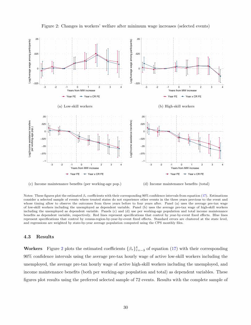
Figure 2: Changes in workers’ welfare after minimum wage increases (selected events)

-.025

0

.025

.05

Log(

Aver

age

wag

e am

ong

parti

cipa

nts)

-3 -2 -1 0 1 2 3 4Years from MW increase

Year FE Year x CR FE

(a) Low-skill workers

-.025

0

.025

.05

Log(

Aver

age

wag

e am

ong

parti

cipa

nts)

-3 -2 -1 0 1 2 3 4Years from MW increase

Year FE Year x CR FE

(b) High-skill workers

-.1

-.075

-.05

-.025

0

.025

.05

Log(

Inco

me

assi

stan

ce tr

ansf

ers

per w

orki

ng-a

ge p

op.)

-3 -2 -1 0 1 2 3 4Years from MW increase

Year FE Year x CR FE

(c) Income maintenance benefits (per working-age pop.)

-.1

-.075

-.05

-.025

0

.025

.05

Log(

Inco

me

assi

stan

ce tr

ansf

ers)

-3 -2 -1 0 1 2 3 4Years from MW increase

Year FE Year x CR FE

(d) Income maintenance benefits (total)

Notes: These figures plot the estimated βτ coefficients with their corresponding 90% confidence intervals from equation (17). Estimationsconsider a selected sample of events where treated states do not experience other events in the three years previous to the event andwhose timing allow to observe the outcomes from three years before to four years after. Panel (a) uses the average pre-tax wageof low-skill workers including the unemployed as dependent variable. Panel (b) uses the average pre-tax wage of high-skill workersincluding the unemployed as dependent variable. Panels (c) and (d) use per working-age population and total income maintenancebenefits as dependent variable, respectively. Red lines represent specifications that control by year-by-event fixed effects. Blue linesrepresent specifications that control by census-region-by-year-by-event fixed effects. Standard errors are clustered at the state level,and regressions are weighted by state-by-year average population computed using the CPS monthly files.

4.3 Results

Workers Figure 2 plots the estimated coefficients {βτ}4τ=−3 of equation (17) with their corresponding

90% confidence intervals using the average pre-tax hourly wage of active low-skill workers including the

unemployed, the average pre-tax hourly wage of active high-skill workers including the unemployed, and

income maintenance benefits (both per working-age population and total) as dependent variables. These

figures plot results using the preferred selected sample of 72 events. Results with the complete sample of

30

Table 2: Worker-level results

(a) Low-skill Workers (b) High-skill Workers

All events Selected events All events Selected events

β 0.025 0.021 0.025 0.014 0.012 0.020 0.002 0.001 0.003 0.000 -0.003 0.001(0.008) (0.008) (0.012) (0.008) (0.010) (0.010) (0.004) (0.003) (0.005) (0.006) (0.005) (0.007)

Year FE Y N N Y N N Y N N Y N NYear x CR FE N Y N N Y N N Y N N Y NYear x CD FE N N Y N N Y N N Y N N YObs. 36613 36613 34797 14860 14860 14099 36613 36613 34797 14860 14860 14099Events 172 172 172 64 64 64 172 172 172 64 64 64∆ log MW 0.101 0.101 0.101 0.128 0.128 0.126 0.101 0.101 0.101 0.128 0.128 0.126Elast. 0.251 0.204 0.242 0.107 0.093 0.160 0.024 0.010 0.034 0.002 -0.022 0.009

(c) Income Maintenance Benefits (d) Income Maintenance Benefits(Per Working-Age Individual) (Total)

All events Selected events All events Selected events

β -0.032 -0.038 -0.038 -0.041 -0.041 -0.046 -0.032 -0.045 -0.038 -0.038 -0.047 -0.045(0.009) (0.006) (0.008) (0.012) (0.009) (0.012) (0.008) (0.008) (0.007) (0.012) (0.011) (0.012)

Year FE Y N N Y N N Y N N Y N NYear x CR FE N Y N N Y N N Y N N Y NYear x CD FE N N Y N N Y N N Y N N YObs. 37749 37749 35914 17604 17604 16818 37749 37749 35914 17604 17604 16818Events 172 172 172 72 72 72 172 172 172 72 72 72∆ log MW 0.101 0.101 0.102 0.127 0.127 0.125 0.101 0.101 0.102 0.127 0.127 0.125Elast. -0.314 -0.374 -0.376 -0.322 -0.322 -0.368 -0.321 -0.449 -0.376 -0.301 -0.367 -0.363

Notes: This table shows the estimated β coefficient from equation (18). All columns represent different regressions using differentdependent variables (all in logarithms), fixed effects, and samples of events. Panel (a) uses the average pre-tax wage of low-skill workersincluding the unemployed as dependent variable. Panel (b) uses the average pre-tax wage of high-skill workers including the unemployedas dependent variable. Panel (c) uses income maintenance benefits per working age individual as dependent variable. Panel (d) usestotal income maintenance benefits as dependent variable. ∆ log MW is the average change in the log of the real state-level minimumwage across events in the year of the event. Elast. is the implied elasticity, that comes from dividing the point estimate by ∆ log MW.Standard errors (in parentheses) are clustered at the state level and regressions are weighted by state-by-year population.

events are presented in Figure C.II of Appendix C.26 Each figure plots regressions with two different types

of time fixed-effects: year-by-event fixed effects and census-region-by-year-by-event fixed effects. Table

2 presents the estimated coefficients β of equation (18) that summarize the average treatment effect in

the post period, considering results using both all and the selected sample of events, and also including

specifications that control for census-division-by-year-by-event fixed effects.

Panel (a) of Figure 2 shows that state-level minimum wage increases have increased the average pre-

tax hourly wage of active low-skill workers including the unemployed. Table 2 shows that the implied

elasticity ranges between 0.09 and 0.16 in the preferred specification, and becomes almost two times larger

when using the full sample of events. Panel (b) of Figure 2 shows that these minimum wage increases have

had null effects on the average pre-tax hourly wage of active high-skill workers including the unemployed.

These results suggest that state-level minimum wages have reduced welfare gaps between low- and high-

skill active workers. Panels (c) and (d) of Figure 2 show that part of the increase in the average pre-tax

hourly wage of active low-skill workers including the unemployed has been offset by a reduction in

26The comparison between Figures 2 and C.II illustrates the tradeoff of using the full set of events versus the restrictedsample. Using all events generate more precise estimates at the cost of inducing small pre-trends, potentially due to thepresence of events in the pre-period. Reassuringly, both strategies yield similar conclusions for all the outcomes considered.

31

Table 3: Additional results for low-skill workers (selected events)

(a) Year-by-event fixed effects

Margins Het.: Age Het.: EducWage Hours Emp. Part. [16,19] [20,30] >30 HS drop. HS comp. Coll. inc.

β 0.014 -0.001 -0.000 -0.003 0.036 0.012 0.010 0.017 0.011 0.015(0.003) (0.004) (0.007) (0.007) (0.012) (0.009) (0.009) (0.012) (0.009) (0.007)

Obs. 14860 14860 14860 14860 14860 14860 14860 14860 14860 14860Events 64 64 64 64 64 64 64 64 64 64∆ log MW 0.128 0.128 0.128 0.128 0.128 0.128 0.128 0.128 0.128 0.128Elast. 0.109 -0.010 -0.002 -0.020 0.283 0.096 0.080 0.135 0.089 0.119

(b) Census-region-by-year-by-event fixed effects

Margins Het.: Age Het.: EducWage Hours Emp. Part. [16,19] [20,30] >30 HS drop. HS comp. Coll. inc.

β 0.012 -0.004 -0.000 -0.005 0.034 0.011 0.009 0.010 0.010 0.015(0.003) (0.004) (0.008) (0.008) (0.012) (0.010) (0.010) (0.013) (0.010) (0.010)

Obs. 14860 14860 14860 14860 14860 14860 14860 14860 14860 14860Events 64 64 64 64 64 64 64 64 64 64∆ log MW 0.128 0.128 0.128 0.128 0.128 0.128 0.128 0.128 0.128 0.128Elast. 0.097 -0.031 -0.004 -0.037 0.267 0.086 0.072 0.075 0.078 0.119

(c) Census-division-by-year-by-event fixed effects

Margins Het.: Age Het.: EducWage Hours Emp. Part. [16,19] [20,30] >30 HS drop. HS comp. Coll. inc.

β 0.011 -0.000 0.009 -0.002 0.042 0.016 0.020 0.025 0.019 0.020(0.003) (0.005) (0.009) (0.011) (0.016) (0.012) (0.011) (0.017) (0.011) (0.011)

Obs. 14099 14099 14099 14099 14099 14099 14099 14099 14099 14099Events 64 64 64 64 64 64 64 64 64 64∆ log MW 0.126 0.126 0.126 0.126 0.126 0.126 0.126 0.126 0.126 0.126Elast. 0.086 -0.002 0.075 -0.017 0.338 0.127 0.156 0.198 0.149 0.159

Notes: This table shows the estimated β coefficient from equation (18) using different dependent variables for low-skill workers (all inlogarithms). Regressions only consider the sample of selected events. Panel (a) uses year-by-event fixed effects. Panel (b) uses census-region-by-year-by-event fixed effects. Panel (c) uses census-division-by-year-by-event fixed effects. Within each panel, columns (1)-(4)decompose the overall effect in four margins: wage (conditional on employment), hours (conditional on employment), employment rate,and participation rate. Columns (5)-(7) use the average pre-tax hourly wage of active low-skill workers including the unemployed thatare between 16 and 19 years old, between 20 and 30 years old, and older than 30, respectively. Columns (8)-(10) use the average pre-taxhourly wage of active low-skill workers including the unemployed that are high school dropouts, have complete high-school education,and have incomplete college education, respectively. ∆ log MW is the average change in the log of the real state-level minimum wageacross events in the year of the event. Elast. is the implied elasticity, that comes from dividing the point estimate by ∆ log MW.Standard errors (in parentheses) are clustered at the state level and regressions are weighted by state-by-year population.

income maintenance benefits. Table 2 shows that the implied elasticity of income maintenance benefits

per working age population ranges between -0.31 and -0.37, depending on the specification. Results are

consistent when using total income maintenance benefits, suggesting that these results are not driven by

changes in the underlying working-age population.

To better understand how minimum wages have affected low-skill workers, Table 3 shows two sets of

complementary results. To simplify exposition, Table 3 only presents results using the selected sample

of events. Results using the full sample of events can be found in Table C.II of Appendix C. The

different panels consider different sets of time fixed effects. Within each panel, columns (1)-(4) decompose

the overall effect on different margins: hourly wage, weekly hours (both conditional on employment),

employment rate, and participation rate. Results indicate that all the effect of minimum wage increases

32

on the average pre-tax hourly wage of active low-skill workers including the unemployed is driven by an

increase in the wage conditional on employment, with no effect on hours, employment, or participation.27

Columns (5)-(7) estimate the main effect on the average pre-tax hourly wage of active workers including

the unemployed for different samples of low-skill workers split by age. The effect is positive for all groups,

but it is between 2 and 3 times larger for teens. This suggests that the coarse aggregation at the skill-level

is possibly underestimating the distributional benefits of the minimum wage since teens are more likely

to work on minimum wage jobs (Manning, 2021; Cengiz et al., 2022). Columns (8)-(10) show that there

is no heterogeneous effect by educational status among the individuals with no college education.

Capitalists Figure 3 plots the estimated coefficients {βτ}4τ=−3 of equation (17) with their correspond-

ing 90% confidence intervals using the gross operating surplus per private establishment as dependent

variable. These figures plot results using the preferred selected sample of 72 events. Results with the com-

plete sample of events are presented in Figure C.III of Appendix C. Each figure plots regressions with two

different types of time fixed-effects: year-by-event fixed effects and census-region-by-year-by-event fixed

effects. Panel (a) shows results aggregating all industries. Panel (b) focuses on non-professional services

–educational services, health care, arts, entertainment, recreation, accomodation, and food services–, a

sector that is usually flagged as having larger shares of minimum wage workers (Card and Krueger, 1994;

Dube et al., 2010; Cengiz et al., 2019; Ruffini, 2021). Regressions are restricted to the 1990-2019 period

to use the industry classification. Table 4 presents the estimated coefficients β of equation (18) that sum-

marize the average treatment effect in the post period, considering results using both all and the selected

sample of events, and also including specifications that control for census-division-by-year-by-event fixed

effects. Table 5 provides a slightly more granular industry-level decomposition of the main result.

Panel (a) shows that there is no effect on profits per establishment when pooling all industries. This is

possibly explained by the fact that minimum wage workers represent a small share of the overall economy.

However, Panel (b) shows that when looking at the non-professional services industry, where the share

of minimum wage workers is larger, there is a negative effect on profits per establishment. Table 4 shows

that the implied elasticity is between -0.12 and -0.21 in the preferred specification.

To further understand the industry-level heterogeneity, Table 5 shows results for a wide range of

industries. To simplify exposition, Table 5 only presents results using the selected sample of events.

Results using the full sample of events can be found in Table C.III of Appendix C. The different panels

consider different sets of time fixed effects. The first two columns replicate the aggregate null effect for

the periods 1979-2019 and 1990-2019 to check that the period selection does not affect the results. The

rest of the columns estimate profit effects for different industries. The non-professional services industry

stands out by displaying consistent negative effect across all specifications. For the other sectors, point

27The lack of employment responses suggests that the result is robust to including curvature in the flow utility of workers.

33

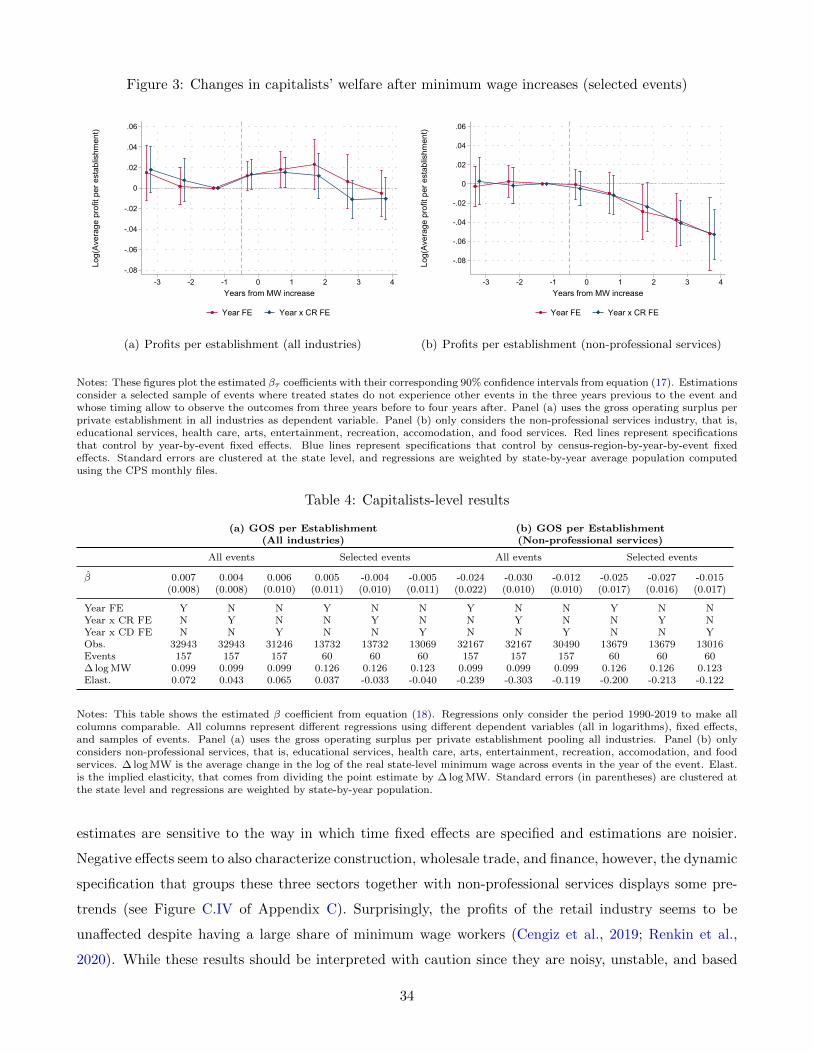
Figure 3: Changes in capitalists’ welfare after minimum wage increases (selected events)

-.08

-.06

-.04

-.02

0

.02

.04

.06

Log(

Aver

age

prof

it pe

r est

ablis

hmen

t)

-3 -2 -1 0 1 2 3 4Years from MW increase

Year FE Year x CR FE

(a) Profits per establishment (all industries)

-.08

-.06

-.04

-.02

0

.02

.04

.06

Log(

Aver

age

prof

it pe

r est

ablis

hmen

t)

-3 -2 -1 0 1 2 3 4Years from MW increase

Year FE Year x CR FE

(b) Profits per establishment (non-professional services)

Notes: These figures plot the estimated βτ coefficients with their corresponding 90% confidence intervals from equation (17). Estimationsconsider a selected sample of events where treated states do not experience other events in the three years previous to the event andwhose timing allow to observe the outcomes from three years before to four years after. Panel (a) uses the gross operating surplus perprivate establishment in all industries as dependent variable. Panel (b) only considers the non-professional services industry, that is,educational services, health care, arts, entertainment, recreation, accomodation, and food services. Red lines represent specificationsthat control by year-by-event fixed effects. Blue lines represent specifications that control by census-region-by-year-by-event fixedeffects. Standard errors are clustered at the state level, and regressions are weighted by state-by-year average population computedusing the CPS monthly files.

Table 4: Capitalists-level results

(a) GOS per Establishment (b) GOS per Establishment(All industries) (Non-professional services)

All events Selected events All events Selected events

β 0.007 0.004 0.006 0.005 -0.004 -0.005 -0.024 -0.030 -0.012 -0.025 -0.027 -0.015(0.008) (0.008) (0.010) (0.011) (0.010) (0.011) (0.022) (0.010) (0.010) (0.017) (0.016) (0.017)

Year FE Y N N Y N N Y N N Y N NYear x CR FE N Y N N Y N N Y N N Y NYear x CD FE N N Y N N Y N N Y N N YObs. 32943 32943 31246 13732 13732 13069 32167 32167 30490 13679 13679 13016Events 157 157 157 60 60 60 157 157 157 60 60 60∆ log MW 0.099 0.099 0.099 0.126 0.126 0.123 0.099 0.099 0.099 0.126 0.126 0.123Elast. 0.072 0.043 0.065 0.037 -0.033 -0.040 -0.239 -0.303 -0.119 -0.200 -0.213 -0.122

Notes: This table shows the estimated β coefficient from equation (18). Regressions only consider the period 1990-2019 to make allcolumns comparable. All columns represent different regressions using different dependent variables (all in logarithms), fixed effects,and samples of events. Panel (a) uses the gross operating surplus per private establishment pooling all industries. Panel (b) onlyconsiders non-professional services, that is, educational services, health care, arts, entertainment, recreation, accomodation, and foodservices. ∆ log MW is the average change in the log of the real state-level minimum wage across events in the year of the event. Elast.is the implied elasticity, that comes from dividing the point estimate by ∆ log MW. Standard errors (in parentheses) are clustered atthe state level and regressions are weighted by state-by-year population.

estimates are sensitive to the way in which time fixed effects are specified and estimations are noisier.

Negative effects seem to also characterize construction, wholesale trade, and finance, however, the dynamic

specification that groups these three sectors together with non-professional services displays some pre-

trends (see Figure C.IV of Appendix C). Surprisingly, the profits of the retail industry seems to be

unaffected despite having a large share of minimum wage workers (Cengiz et al., 2019; Renkin et al.,

2020). While these results should be interpreted with caution since they are noisy, unstable, and based

34

Table 5: Industry heterogeneity (selected events)

(a) Year-by-event fixed effects

All All NNRR Constr. Manuf. Transp. Wholesale Retail Finance Prof. serv Non-prof. serv.

β 0.002 0.005 0.032 -0.013 0.058 0.016 -0.027 0.011 -0.013 0.029 -0.025(0.008) (0.011) (0.036) (0.041) (0.040) (0.032) (0.024) (0.014) (0.015) (0.013) (0.017)

Obs. 17604 13732 13328 13677 13666 13682 13732 13732 13732 13732 13679Events 72 60 60 60 60 60 60 60 60 60 60∆ log MW 0.127 0.126 0.127 0.126 0.126 0.126 0.126 0.126 0.126 0.126 0.126Elast. 0.015 0.037 0.251 -0.100 0.457 0.125 -0.211 0.090 -0.101 0.234 -0.200

(b) Census-region-by-year-by-event fixed effects

All All NNRR Constr. Manuf. Transp. Wholesale Retail Finance Prof. serv Non-prof. serv.

β -0.003 -0.004 0.007 -0.057 0.050 -0.005 -0.041 -0.006 -0.017 0.019 -0.027(0.009) (0.010) (0.033) (0.043) (0.041) (0.030) (0.024) (0.014) (0.013) (0.012) (0.016)

Obs. 17604 13732 13285 13677 13666 13682 13732 13732 13732 13732 13679Events 72 60 60 60 60 60 60 60 60 60 60∆ log MW 0.127 0.126 0.127 0.126 0.126 0.126 0.126 0.126 0.126 0.126 0.126Elast. -0.023 -0.033 0.056 -0.456 0.395 -0.042 -0.323 -0.045 -0.135 0.150 -0.213

(c) Census-division-by-year-by-event fixed effects

All All NNRR Constr. Manuf. Transp. Wholesale Retail Finance Prof. serv Non-prof. serv.

β -0.003 -0.005 -0.042 -0.047 0.023 -0.045 0.008 0.005 -0.020 0.006 -0.015(0.011) (0.011) (0.038) (0.045) (0.039) (0.025) (0.027) (0.013) (0.014) (0.017) (0.017)

Obs. 16818 13069 12605 13012 13003 13019 13069 13069 13069 13069 13016Events 72 60 60 60 60 60 60 60 60 60 60∆ log MW 0.125 0.123 0.124 0.123 0.123 0.123 0.123 0.123 0.123 0.123 0.123Elast. -0.020 -0.040 -0.338 -0.382 0.186 -0.362 0.069 0.040 -0.163 0.049 -0.122

Notes: This table shows the estimated β coefficient from equation (18) using the gross operating surplus per private establishmentfor different industries (all in logarithms) using census-division-by-year-by-event fixed effects. Regressions only consider the sampleof selected events. Panel (a) uses year-by-event fixed effects. Panel (b) uses census-region-by-year-by-event fixed effects. Panel(c) uses census-division-by-year-by-event fixed effects. NNRR includes agriculture, forestry, fishing, hunting, and mining. Constr.includes construction. Manuf. includes durable and nondurable goods manufacturing. Transp. includes transportation. Wholesaleincludes wholesale trade. Retail includes retail trade. Finance includes finance, insurance, real estate, rental, and leasing. Prof. serv.includes professional and business services. Non-prof. serv. includes educational services, health care, arts, entertainment, recreation,accomodation, and food services. ∆ log MW is the average change in the log of the real state-level minimum wage across events inthe year of the event. Elast. is the implied elasticity, that comes from dividing the point estimate by ∆ log MW. Standard errors (inparentheses) are clustered at the state level and regressions are weighted by state-by-year population.

on non-ideal aggregate data of profits, they suggest that industry heterogeneity matters for the effects

on the capitalists’ side and call for a more thorough analysis based on firm-level microdata.

Related literature The results on workers’ outcomes are consistent with Cengiz et al. (2019, 2022)

who find positive wage effects, limited employment effects, and limited participation effects in the part of

the distribution close to the minimum wage using similar data and empirical strategy. Those findings are

common in the related literature (Manning, 2021). While consistent, my results differ from theirs along

two dimensions. First, I focus on wider skill groups that are not exactly composed by minimum wage

workers. Second, the main focus of my analysis is the estimation of the composite sufficient statistic rather

than the effect on different margins. The effects on income maintenance benefits are consistent with Reich

and West (2015) and Dube (2019) who also find reductions in transfer spending after minimum wage

increases. The effects on capitalists are, to my knowledge, the first profit elasticities estimated for the

US and, while noisy and only suggestive, are qualitatively consistent with estimations for other countries

35

based on granural firm-level data. Draca et al. (2011) study the introduction of the national minimum

wage in the United Kingdom and find that profit margins fell by almost 30%. Harasztosi and Lindner

(2019) find that profits fell around 1% after a large minimum wage increase in Hungary. This decrease

represented around 30% of the average profitability in the pre-reform year. Drucker et al. (2021) study

the Israeli case and finds a reduction of 7.5% in profits of highly exposed firms.

With respect to the recent structural literature that focus on the distributional impacts of the mini-

mum wage, my results are consistent with the quantitative exercise in Berger et al. (2022b) that suggests

that welfare gains are concentrated in workers and decreasing in skill, while welfare losses are concen-

trated in capital owners. My results also relate to Hurst et al. (2022) simulations. They find positive

aggregate effects on low-skill workers, but argue that within low-skill workers the ones at the bottom of

the distribution are made worse off by the policy. My results differ from theirs since I find larger welfare

increases for teens, which are more likely to be at the bottom of the distribution conditional on being

low-skill. It should be kept in mind that both set of results are not fully comparable since Hurst et al.

(2022) analysis focuses on the long-run consequences of the minimum wage increase (i.e., 15-20 years

after the policy change). The long-run analysis is beyond the scope of this paper.

4.4 Back to the optimal policy analysis

The empirical results inform about the effects of minimum wages on low-skill workers, high-skill workers,

and capitalits’ welfare. However, the estimated elasticities are not sufficient to draw conclusions on the

overall desirability of the minimum wage. Recall from Section 3 that to assess if increasing the minimum

wage is welfare-improving, the social planner needs information on the social value of the welfare changes

on active low-skill workers, the social value of the welfare changes on active high-skill workers, the

social value of the welfare changes on active capitalists, and the fiscal externalities on both workers’ and

capitalists’ sides. Results so far only depict an incomplete picture of this analysis. The remainder of the

section uses the estimated elasticities to develop a simple calibration of Proposition II to get additional

insights about the welfare properties of the minimum wage policy.

Revisiting Proposition II Consider the following modified version of equation (14). When taxes are

fixed, increasing the minimum wage increases aggregate welfare if

d logU l

dw· U l · LlA · gl1 +KA · (1− t) ·

∫ ψ

ψ∗gψd log Π(ψ)

dwΠ(ψ)dO(ψ) + Fiscal effects > 0, (19)

where KA = K · (1−O(ψ∗)), O(ψ) = O(ψ)/(1−O(ψ∗)), and the fiscal effects consider both workers’ and

capitalists’ sides fiscal externalities. The high-skill workers component is omitted since the estimations

of Table 2 suggest that dUh/dw = 0.

36

On the workers’ side, note from equation (13) that

U l · LlA =

∫Elmw

lmdm−

∫ElmT (wlm)dm+ y0 · LlA · ρl, (20)

that is, U l ·LlA is equal to total pre-tax income (first term) plus the net tax liabilities, which are composed

by the taxes paid by employed workers (second term) and the transfers received by the unemployed

workers. Total pre-tax annual income of employed low-skill workers can be computed using the CPS-

MORG data. Since taxes paid at the bottom of the distribution are possibly negative, I use the total

income maintenance benefits from the BEA regional accounts as a proxy for total net tax liabilities of

low-skill workers. Then, the low-skill workers’ side component of (19) can be written as

d logU l

dw· U l · LlA · gl1 = εU l · (TPTW + TIMB) · gl1, (21)

where εU l ≡ d logU l/dw, TPTW accounts for total annual pre-tax wages, and TIMB accounts for total

income maintenance benefits.

On the capitalists’ side, I impose that εΠ ≡ d log Π(ψ)/dw is constant given the lack of firm-level

microdata needed to estimate heterogeneous effects. Denoting as Π the (unweighted) average pre-tax

profit of active firms, the capitalists’ side component of (19) can be written as

KA · (1− t) ·∫ ψ

ψ∗gψd log Π(ψ)

dwΠ(ψ)dO(ψ) = εΠ · TPTP · (1− t) · gK , (22)

where TPTP = KA · Π accounts for total pre-tax profits and gK =∫ ψψ∗ gψ

Π(ψ)

ΠdO(ψ) is the average

SMWW across active capitalists. TPTP can be computed using the data of the empirical analysis.

Finally, fiscal effects can be decomposed into workers’ side and capitalists’ side fiscal externali-

ties. I proxy workers’ side effects by the change in TIMB, with a corresponding semi-elasticity of

εB ≡ d log TIMB/dw. On the capitalists’ side, I assume that fiscal externalities are well approximated

by the loss in the corporate tax revenue due to the effects on profits.28 Then

Fiscal effects = −εB · TIMB + εΠ · t · TPTP. (23)

28This claim has two caveats. First, changes in the number of establishments can also generate a fiscal externality. Second,changes in corporate profits may affect personal income tax collection either through reported business income, dividends,or S-corps income. In Table C.IV of Appendix C I show that minimum wages do not predict changes in these margins, sothe fiscal externalities of capitalists are well approximated by changes in pre-tax profits. The number of establishments, ifanything, shows a small but non-significant increase after minimum wage changes. Business income, dividend income, andS-Corp income reported in SOI state-level public tables do not change after minimum wage increases, neither at the intensive(per return or per working age population) or extensive (number of returns with positive income) margins.

37

Then, (19) can be written as

εU l · (TPTW + TIMB) · gl1 + εΠ · TPTP · (1− t) · gK − εB · TIMB + εΠ · t · TPTP > 0. (24)

Recall that Proposition II characterizes conditions under which small increases of the minimum wage

are welfare-improving. This can be quantitatively assessed by imputing values to the components of the

left-hand-side of (24). From equation (24), it can also be computed the minimum SMWW on active

low-skill workers that make the condition true, that is

gl∗1 =−εΠ · TPTP · (1− t) · gK + εB · TIMB− εΠ · t · TPTP

εU l · (TPTW + TIMB), (25)

where gl∗1 is the critical SMWW on active low-skill workers. Holding fix the rest of the components, any

gl1 ≥ gl∗1 makes the minimum wage increase desirable for redistribution. Then, gl∗1 is a measure of the

restrictions on social preferences for redistribution that make the policy change desirable. The smaller

gl∗1 , the weaker the required preferences for redistribution toward low-skill workers.

Calibration Calibration of equation (24) requires estimating four sets of components: (i) the monetary

aggregates, {TPTW,TIMB,TPTP}, (ii) the semi-elasticities, {εU l , εΠ, εB}, (iii) the corporate tax rate, t,

and (iv) the SMWWs, {gl1, gK}. Below I describe the steps followed to compute each of these components.

Appendix D provides additional details about the calculations.

Values for {TPTW,TIMB,TPTP} can be directly computed from the data used in the empirical

analysis. I use two assumptions for their computation: (i) the population weighted average values of

pre-event years across treated states, and (ii) the population weighted average values for 2019. The

former calculation is used to assess past minimum wage increases. The latter is used to speculate about

small minimum wage increases today. For TPTP, I only consider the industries that were found to have

negative profit effects, namely non-professional services, construction, wholesale trade.

Values for {εU l , εΠ, εB} can be recovered from Tables 2 and 5. εΠ corresponds to the semi-elasticity

of profits per establishment of each of the considered industries. εB corresponds to the semi-elasticity

of total income maintenance benefits. Since εU l accounts for changes in post-tax values, it cannot be

directly recovered from Table 2. I proceed as follows. First, I add the values for TPTW and TIMB

to estimate total post-tax incomes of active low-skill workers including the unemployed. Then, I apply

the estimated semi-elasticities of Table 2 separately for the TPTW and TIMB components to estimate

the total post-tax incomes of active low-skill workers including the unemployed after the minimum wage

increase. Finally, I compute the percent change of the estimated post-tax incomes to recover εU l . Since

some of the semi-elasticities are sensitive to the inclusion of different time fixed effects, I calibrate equation

(24) using different values for {εU l , εΠ, εB} that come from the different empirical models.

38

The value for the corporate tax rate, t, is computed based on observed US corporate tax rates. I con-

sider two cases. First, I consider the statutory corporate tax rate. I set t = 35% when using the population

weighted average value of pre-event years across treated states to compute {TPTW,TIMB,TPTP}, which

is the tax rate that applied between 1993 and 2017, and t = 21% when using the population weighted

average values for 2019 to compute {TPTW,TIMB,TPTP}, which is the current statutory corporate tax

rate. Second, I consider measures of effective corporate tax rates following Zucman (2014).29 For the

first case I set t = 23%, which is the average value for the period 1979-2017. In the second case I consider

t = 13%, which is the most recent value of the series.

Finally, values {gl1, gK} are computed using two approaches. First, I consider gl1 = gK = 1. This

represents a case with no redistributive considerations so the welfare calculation is reduced to computing

changes in total output. This benchmark can be thought of as a test for the efficiency of the labor

market. Second, I follow the optimal taxation literature with endogenous SMWWs (e.g., Mirrlees, 1971;

Saez, 2001; Piketty and Saez, 2013) and add structure to the framework presented in Section 3 by

assuming that the G function of the social welfare criterion is CRRA, that is, that G(V ) = V 1−ζ/(1− ζ),

with ζ > 0 and preferences for redistribution increasing in ζ. This functional form allows to calculate

gl1/gK using (powers of) the ratio of average post-tax incomes. Denote by ω(ζ) = gl(ζ)/gK(ζ) the ratio

of average SMWWs given ζ, where ω(ζ) is proportional to the ratio of average post-tax incomes (see

Appendix D).30 I set gl1 = 1 and gK = 1/ω(ζ), which converges to gK = 0 when average profits are order

of magnitudes larger than the average incomes of workers. This latter limit case matches the normative

assumption that is implicit in most of the related literature where the desirability of the policy is assessed

by only looking at worker-level outcomes.

For a given calibration choice, I perform two complementary exercises. First, I check whether equation

(24) holds. This informs about the desirability of the minimum wage for redistributive purposes holding

gl1 = 1 fixed. Second, I use (25) to compute gl∗1 and inform about the required preference for redistribution

that would make the minimum wage increase welfare-improving.31 This also informs by how far equation

(24) holds or not.

Results Table 6 summarizes the results. Each cell considers a different permutation of the calibration

choices discussed above to answer (i) whether equation (24) holds when gl1 is normalized to 1, and

(ii) the value of gl∗1 . The three panels use different values for the semi-elasticities, {εU l , εΠ, εB}, taken

29Effective corporate tax rates are computed by dividing all the corporate taxes paid by US firms (to US and foreigngovernments) by total US corporate profits using national accounts data taken from the BEA NIPA tables.

30For simplicity, I do not consider the participation and entry costs that ultimately matter for the computation of theSMWWs. Given Jensen’s inequality, to the extent that entry costs for firms do not represent a much more larger share ofprofits than search costs represent for low-skill workers average incomes (including the unemployed), abstracting for themimplies that the calibration of ω(ζ) is possibly a lower bound.

31Equation (25) is slightly different in the case of endogenous SMWWs because gK is a function of gl1. See Appendix D.

39

Table 6: Quantitative calibration of Proposition II

(a) Semi-elasticities of models with year-by-event fixed effects

Past minimum wage increases Minimum wage increases today

gK : gK :1 1/ω(1) 1/ω(1.5) 1/ω(2) 1 1/ω(1) 1/ω(1.5) 1/ω(2)

Statutory t Is (24) true? 3 3 3 3 3 3 3 3

gl∗1 0.533 0.118 0.116 0.115 0.642 0.061 0.060 0.060

Effective t Is (24) true? 3 3 3 3 3 3 3 3

gl∗1 0.533 0.039 0.038 0.038 0.642 0.001 0.001 0.001

(b) Semi-elasticities of models with census-region-by-year-by-event fixed effects

Past minimum wage increases Minimum wage increases today

gK : gK :1 1/ω(1) 1/ω(1.5) 1/ω(2) 1 1/ω(1) 1/ω(1.5) 1/ω(2)

Statutory t Is (24) true? 3 3 3 3 7 3 3 3

gl∗1 0.961 0.237 0.231 0.229 1.167 0.137 0.133 0.132

Effective t Is (24) true? 3 3 3 3 7 3 3 3

gl∗1 0.961 0.097 0.094 0.093 1.167 0.028 0.027 0.027

(c) Semi-elasticities of models with census-division-by-year-by-event fixed effects

Past minimum wage increases Minimum wage increases today

gK : gK :1 1/ω(1) 1/ω(1.5) 1/ω(2) 1 1/ω(1) 1/ω(1.5) 1/ω(2)

Statutory t Is (24) true? 3 3 3 3 3 3 3 3

gl∗1 0.456 0.103 0.102 0.102 0.531 0.051 0.051 0.051

Effective t Is (24) true? 3 3 3 3 3 3 3 3

gl∗1 0.456 0.037 0.036 0.036 0.531 0.002 0.002 0.002

Notes: This table shows whether equation (24) holds and the corresponding estimate of gl∗1 for different calibration choices. Thedifferent panels use different values for the semi-elasticities, {εUl , εΠ, εB}, taken from different estimated models in Tables 2 and 5 thatvary in the time fixed effects considered. Within each panel, the left sub-panel uses the population weighted average values of pre-eventyears across all treated states considered in the empirical analysis to estimate {TPTW,TIMB,TPTP}, while the right sub-panel usesthe population weighted averages of 2019. Within each sub-panel, columns consider the different approaches for computing gK , wherethe first column sets gK = 1 and the other three compute gK = 1/ω(ζ) for ζ ∈ {1, 1.5, 2}. Also, within each sub-panel, the rowsconsider either the statutory corporate tax rate or the effective corporate tax rate. The statutory and effective corporate tax rates are(35%, 23%) in the left sub-panel and (21%, 13%) in the right sub-panel, respectively. Additional details of the calibration can be foundin Appendix D.

from the different estimated models using the selected sample of events of Tables 2 and 5 that vary in

the time fixed effects considered. Within each panel, the left sub-panel uses the population weighted

average values of pre-event years across all treated states considered in the empirical analysis to estimate

{TPTW,TIMB,TPTP}, so the analysis assess the welfare implications of past-minimum wage increases,

while the right sub-panel uses the population weighted averages of 2019, so it speculates about the

welfare implications of hypothetical minimum wage increases today. Within each sub-panel, columns

consider the different approaches for computing gK , where the first column sets gK = 1 (so distributional

considerations are muted) and the other three compute gK = 1/ω(ζ) for ζ ∈ {1, 1.5, 2}. Also, within each

sub-panel, the rows consider either the statutory corporate tax rate or the effective corporate tax rate.

Table 6 shows that equation (24) is true in almost all cases. That is, past minimum wage increases

have been welfare improving, and small minimum wage increases today are likely to be as well. This is

40

also true for 10 out of the 12 cases in which gK = 1, implying that the efficient benchmark is rejected in

most cases: the increase in post-tax incomes for low-skill workers including the unemployed more than

compensates the fall in profits. Total output seems to have increased after minimum wage increases.

One important aspect of Table 6 is that gl∗1 decreases considerably when distributional concerns are

incorporated through gK . That is, the minimum SMWW for low-skill workers that makes a case for the

minimum wage is an order of magnitude smaller when the increases in after-tax incomes for low-skill

workers have a larger social value than the profit losses. Even when total output falls, the incorporation

of distributional concerns makes the case for the minimum wage unambiguously favorable. Interestingly,

the degree of concavity of the social welfare function, ζ, which measures the strength of the social

preferences for redistribution, does not affect the analysis. This is mainly driven by the fact that average

post-tax profits are several times larger than average post-tax incomes of active low-skill workers, so the

redistributive forces in (24) manifest even when the concavity of the social welfare function is moderate.

The corporate tax rate plays an important role in the analysis. Within each sub-panel, gl∗1 is larger

when considering the statutory tax rate, which is larger than the effective tax rate.32 The reason is that

the larger the corporate tax rate, the larger the corporate tax revenue loss, which matters for welfare

regardless of the social value put on capitalists’ incomes. This reinforces the narrative developed in

Section 3: if international tax competition is pushing tax rates down, the minimum wage can mimic

sector-specific tax rates to redistribute profits from labor-intensive industries to workers.

Comparing the analysis of past minimum wage increases to hypothetical future ones provide two

additional insights. First, when gK = 1, the estimated gl∗1 is larger for assessing minimum wage increases

today. That is, absent distributional concerns based on relative incomes, conditions on social preferences

are stricter today than they were for past minimum wage increases. This suggests that the potential

efficiency gains today are smaller than the ones that were expected in the past, which is consistent with

past minimum wage increases actually being efficiency enhancing. Second, when distributional concerns

between labor and capital are incorporated through endogenous SMWWs, the case for minimum wage

increases is stronger today than in the past. This is mainly explained by two reasons. First, the disparity

in average incomes between workers and capitalists is larger today than in the past. Second, the corporate

tax rates –both statutory and effective– are smaller today than in the past. Both elements favor the use

of the minimum wage for redistributive purposes.

MVPF The calibrated components of equation (24) can also be used to compute an alternative measure

of the welfare impacts of the minimum wage: the Marginal Value of Public Funds (MVPF) (Finkelstein

and Hendren, 2020; Hendren and Sprung-Keyser, 2020). The MVPF of a policy is an indicator of its

efficacy that compares its benefits to its costs, where the former is measured as the willingness to pay of

32This is true for all cases except when gK = 1. In that case the corporate tax rate plays no role because the fiscalexternality is exactly offset by the welfare effects of the corporate tax payment.

41

Table 7: Marginal Value of Public Funds

(a) Year FE (b) Year x CR FE (c) Year x CD FE

Past minimum Minimum wage Past minimum Minimum wage Past minimum Minimum wagewage increases increases today wage increases increases today wage increases increases today

Stat. t Eff. t Stat. t Eff. t Stat. t Eff. t Stat. t Eff. t Stat. t Eff. t Stat. t Eff. t

MVPFL 7.43 22.58 14.06 1,002.32 3.50 8.62 6.49 32.13 8.63 24.32 17.98 473.63

MVPFK -3.63 -13.07 -9.73 -717.88 -3.22 -9.38 -7.88 -42.94 -3.50 -11.67 -9.50 -275.66

MVPF 3.80 9.51 5.23 284.44 0.29 -0.76 -1.39 -10.81 5.13 12.65 8.48 197.7

Notes: This table presents estimations of MVPFL, MVPFK , and MVPF for different calibration choices, defined as MVPFL =WTPL/Costs, MVPFK = WTPK/Costs, and MVPF = (WTPL + WTPK)/Costs, where Costs = −εΠ · t · TPTP + εB · TIMB,WTPL = εUl ·TPTW + εB ·TIMB, and WTPK = εΠ · (1− t) ·TPTP. The different panels use different values for the semi-elasticities,{εUl , εΠ, εB}, taken from different estimated models in Tables 2 and 5 that vary in the time fixed effects considered. Within each panel,the left sub-panel uses the population weighted average values of pre-event years across all treated states considered in the empiricalanalysis to estimate {TPTW,TIMB,TPTP}, while the right sub-panel uses the population weighted averages of 2019. Within eachsub-panel, the rows consider either the statutory corporate tax rate or the effective corporate tax rate. The statutory and effectivecorporate tax rates are (35%, 23%) in the left sub-panel and (21%, 13%) in the right sub-panel, respectively. Additional details of thecalibration can be found in Appendix D.

the beneficiaries and the latter includes both the direct costs and the fiscal externalities. I can compute

the MVPF of the minimum wage since (i) all utility changes are money-metric and, therefore, can be

interpreted as willingness-to-pay, and (ii) the estimated macro elasticities include all general equilibrium

effects of the policy, including the fiscal externalities.

While minimum wage increases do not have direct costs for the government in terms of spending,

they induce changes on the government’s budget through the fiscal externalities. The costs of the policy

are given by Costs = −εΠ · t ·TPTP + εB ·TIMB, that is, by the loss in the corporate tax revenue net of

the savings due to the reduction in income maintenance benefits.

On the benefits side, workers’ willingness to pay for the increase in the minimum wage is given by

WTPL = εU l · TPTW + εB · TIMB, that is, by the net-increase in after-tax incomes, which corresponds

to the annualized increase in pre-tax wages net of the decrease in income maintenance benefits. Since

profits decrease after minimum wage increases, capitalists are willing to pay to avoid the policy. This

is equivalent to say that their willingness to pay is negative and equal to WTPK = εΠ · (1 − t) · TPTP.

The standard formulation of the MVPF abstracts from SMWWs and restricts the attention to comparing

total net benefits to total net costs, so is given by MVPF = (WTPL + WTPK)/Costs. Alternatively, one

could compute versions that either focus on workers, MVPFL = WTPL/Costs, or capitalits, MVPFK =

WTPK/Costs, when assessing the benefits of the policy.

Table 7 presents estimations of MVPFL, MVPFK , and MVPF for each of the cases considered in

Table 6. As a benchmark, Hendren and Sprung-Keyser (2020) estimates a MVPF of 0.75 for the SSI,

between 0.9 and 1.05 for the SNAP, and between 1.1 and 1.2 for the EITC. The MVPF is larger than 1

in 8 out of 12 cases, meaning that even when abstracting from distributional considerations, the benefits

of the policy seem to outweigh the fiscal costs. The only cases in which the MVPF is below 1 or negative

is when using the semi-elasticities from models with census-region-by-year-by-event fixed effects, since

42

those models predict larger decreases in profits, so the negative willingness to pay of capitalists increase.

The MVPFL is always far larger than one, suggesting that when only workers’ welfare is considered

for computing the benefits the policy is very cost effective, especially when considering the alternatives

such as the SSI, SNAP, or the EITC. The converse is true for the MVPFK . This, again, calls for the

importance of considering distributional concerns where there are clear winners and losers after a policy

implementation. When the MVPF and the MVPFL are above 1, their value is negatively correlated with

the corporate tax rate considered because the cost of the policy is proportional to the corporate tax rate.

This reinforces the narrative of minimum wage increases being more appealing for redistribution when

corporate tax rates are small.

Caveats The calibration analysis is only suggestive. On a conceptual level, recall that Proposition II

studies the desirability of the minimum wage when taxes are fixed. Then, the analysis does not inform

whether the minimum wage is desirable if taxes are optimal and how the tax system can be reformed

to approach its optimal design. That analysis requires information on the micro version of the semi

elasticities which cannot be estimated with the empirical setting of this paper. Also, even if assuming

fixed taxes is the policy-relevant scenario for assessing policy changes, the analysis is local in the sense

that informs about small minimum wage increases. That is, Tables 6 and 7 do not provide information

about how large is the optimal minimum wage.

On a technical level, the analysis assumes that the estimated semi-elasticities are valid today, which

is not necessarily the case if some of the fundamentals have changed over time. Also, given the lack of

firm-level micro data, the analysis abstracts from within-capitalist variation in profits that could play a

role in the distributional consequences of the policy if profit elasticities are not constant (e.g., Drucker

et al., 2021). Finally, elasticities are estimated using non-ideal aggregate data, yielding some results that

are noisy and sensitive to the inclusion of different sets of time fixed effects.

With this in mind, this calibration analysis constitutes a first-step toward a more comprehensive

understanding of the redistributive consequences of the minimum wage, especially when the relationship

between labor and capital is considered. Better data and policy experiments can provide more precise

assessments on the distributional consequences of hypothetical future minimum wage increases, a pressing

issue in the current policy debate.

5 Conclusion

A large literature studies the labor market effects of the minimum wage, usually finding important wage

effects with limited employment consequences. A smaller literature builds on these empirical findings to

understand the role of the minimum wage in the optimal redistributive policy mix, especially when taxes

43

and transfers are available for policymakers. This paper aims to contribute to this latter discussion.

The paper proposes a tractable model of the labor market to develop an optimal policy analysis.

The model features two-sided heterogeneity, has positive firm profits in equilibrium, reproduces several

facts of low-wage labor markets, and predicts realistic effects of minimum wage increases. Additional

modelling choices make the framework especially appealing for understanding the distributional impacts

of the minimum wage, on top of the widely studied potential efficiency-enhancing effects.

With the model of the labor market, the paper then develops an optimal policy analysis to characterize

the effects of the minimum wage on the relative welfare of low-skill workers, high-skill workers, and

capitalists as a function of sufficient statistics for welfare, social preferences for redistribution, and fiscal

externalities. One important insight of the analysis is that the minimum wage can be a useful tool

for redistributing from capital to labor when exogenous forces –such as international tax competition–

prevent social planners to enforce large corporate tax rates. This argument is reinforced after noting that

the profit effects are concentrated on labor-intensive service industries. I also show that the ability of

the minimum wage to shift the incidence of the tax system implies that there may be a role for binding

minimum wages even when the tax system is optimal.

The sufficient statistics that guide the welfare analysis are estimated using state-level variation in

minimum wages. I find that minimum wages have increased low-skill workers’ welfare –especially for

teens– with no effects on high-skill workers. Part of this effect is offset by a decrease in income main-

tenance benefits. Profits of labor-intensive industries also seem to decrease after minimum wage hikes.

The estimated coefficients are used to calibrate a simple welfare analysis that shows that incorporating

distributional concerns to the analysis, especially between labor and capital, is first-order for assessing

the desirability of the minimum wage. While only suggestive, the analysis finds that past minimum wage

increases have increased aggregate US welfare and that small future increases are likely to do that as well.

44

Bibliography

Aaronson, D., E. French, I. Sorkin, and T. To (2018). Industry dynamics and the minimum wage: A

putty-clay approach. International Economic Review 59 (1), 51–84.

Acemoglu, D. (2001). Good jobs versus bad jobs. Journal of Labor Economics 19 (1), 1–21.

Acemoglu, D. and J. S. Pischke (1999). The structure of wages and investment in general training.

Journal of Political Economy 107 (3), 539–572.

Acemoglu, D. and P. Restrepo (2019). Automation and new tasks: How technology displaces and rein-

states labor. Journal of Economic Perspectives 33 (2), 3–30.

Ahlfeldt, G. M., D. Roth, and T. Seidel (2018). The regional effects of Germany’s national minimum

wage. Economics Letters 172, 127–130.

Ahlfeldt, G. M., D. Roth, and T. Seidel (2022). Optimal minimum wages. Working Paper .

Allegretto, S. and M. Reich (2018). Are local minimum wages absorbed by price increases? Estimates

from internet-based restaurant menus. ILR Review 71 (1), 35–63.

Alvaredo, F., A. B. Atkinson, T. Piketty, and E. Saez (2013). The top 1 percent in international and

historical perspective. Journal of Economic Perspectives 27 (3), 3–20.

Andreoni, J., B. Erard, and J. Feinstein (1998). Tax compliance. Journal of Economic Literature 36 (2),

818–860.

Ashenfelter, O. and S. Jurajda (2022). Minimum wages, wages, and price pass-through: The case of

McDonald’s Restaurants. Journal of Labor Economics 40 (S1), S179—-S201.

Atesagaoglu, O. E. and H. Yazici (2021). Optimal taxation of capital in the presence of declining labor

share. Working Paper .

Atkinson, A. B. and J. E. Stiglitz (1976). The design of tax structure: Direct versus indirect taxation.

Journal of Public Economics 6 (1-2), 55–75.

Autor, D. (2015). Why are there still so many jobs? The history and future of workplace automation.

Journal of Economic Perspectives 29 (3), 3–30.

Autor, D., A. Manning, and C. L. Smith (2016). The contribution of the minimum wage to US wage

inequality over three decades: A reassessment. American Economic Journal: Applied Economics 8 (1),

58–99.

45

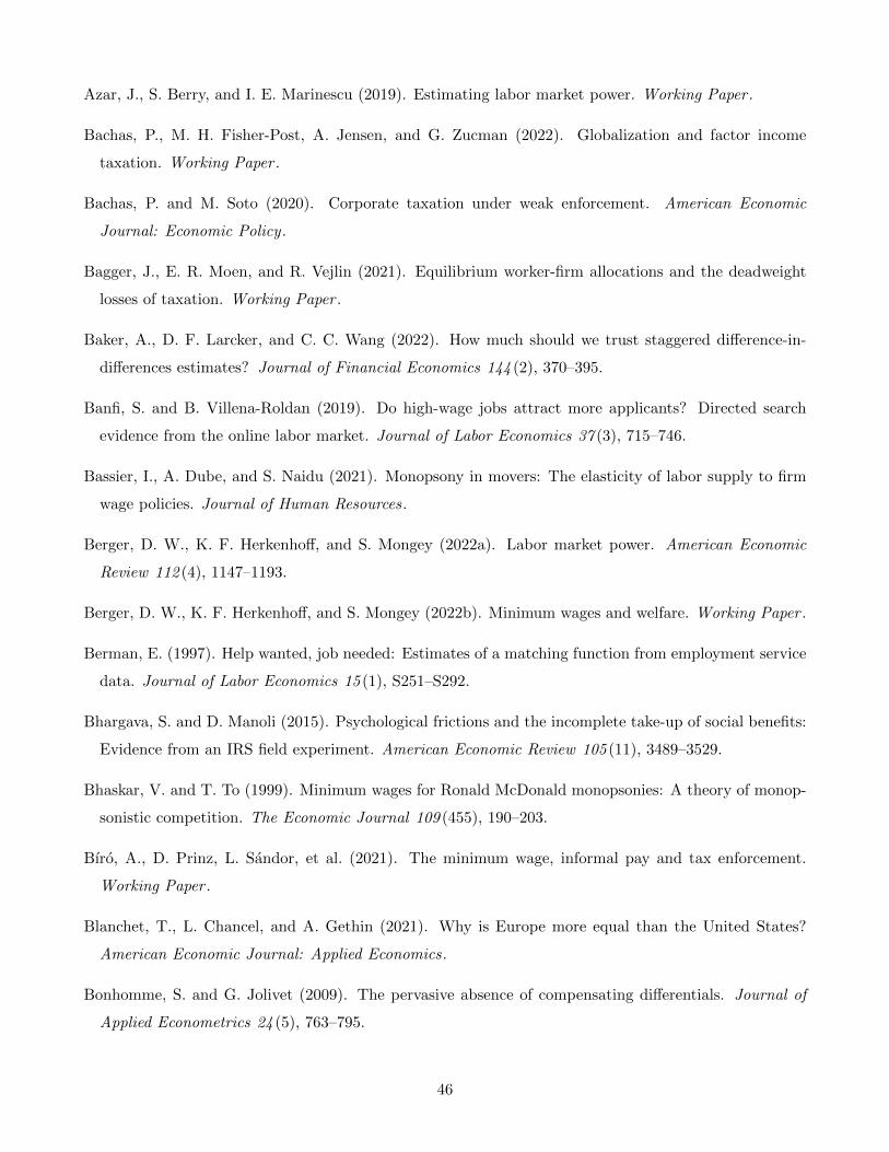
Azar, J., S. Berry, and I. E. Marinescu (2019). Estimating labor market power. Working Paper .

Bachas, P., M. H. Fisher-Post, A. Jensen, and G. Zucman (2022). Globalization and factor income

taxation. Working Paper .

Bachas, P. and M. Soto (2020). Corporate taxation under weak enforcement. American Economic

Journal: Economic Policy .

Bagger, J., E. R. Moen, and R. Vejlin (2021). Equilibrium worker-firm allocations and the deadweight

losses of taxation. Working Paper .

Baker, A., D. F. Larcker, and C. C. Wang (2022). How much should we trust staggered difference-in-

differences estimates? Journal of Financial Economics 144 (2), 370–395.

Banfi, S. and B. Villena-Roldan (2019). Do high-wage jobs attract more applicants? Directed search

evidence from the online labor market. Journal of Labor Economics 37 (3), 715–746.

Bassier, I., A. Dube, and S. Naidu (2021). Monopsony in movers: The elasticity of labor supply to firm

wage policies. Journal of Human Resources.

Berger, D. W., K. F. Herkenhoff, and S. Mongey (2022a). Labor market power. American Economic

Review 112 (4), 1147–1193.

Berger, D. W., K. F. Herkenhoff, and S. Mongey (2022b). Minimum wages and welfare. Working Paper .

Berman, E. (1997). Help wanted, job needed: Estimates of a matching function from employment service

data. Journal of Labor Economics 15 (1), S251–S292.

Bhargava, S. and D. Manoli (2015). Psychological frictions and the incomplete take-up of social benefits:

Evidence from an IRS field experiment. American Economic Review 105 (11), 3489–3529.

Bhaskar, V. and T. To (1999). Minimum wages for Ronald McDonald monopsonies: A theory of monop-

sonistic competition. The Economic Journal 109 (455), 190–203.

Bıro, A., D. Prinz, L. Sandor, et al. (2021). The minimum wage, informal pay and tax enforcement.

Working Paper .

Blanchet, T., L. Chancel, and A. Gethin (2021). Why is Europe more equal than the United States?

American Economic Journal: Applied Economics.

Bonhomme, S. and G. Jolivet (2009). The pervasive absence of compensating differentials. Journal of

Applied Econometrics 24 (5), 763–795.

46

Bosch, M. and M. Manacorda (2010). Minimum wages and earnings inequality in urban Mexico. American

Economic Journal: Applied Economics 2 (4), 128–49.

Bozio, A., J. Goupille-Lebret, and M. Guillot (2020). Predistribution vs. redistribution: Evidence from

France and the US. Working Paper .

Burdett, K. and D. T. Mortensen (1998). Wage differentials, employer size, and unemployment. Inter-

national Economic Review , 257–273.

Butschek, S. (2022). Raising the bar: Minimum wages and employers’ hiring standards. American

Economic Journal: Economic Policy .

Cahuc, P. and G. Laroque (2014). Optimal taxation and monopsonistic labor market: Does monopsony

justify the minimum wage? Journal of Public Economic Theory 16 (2), 259–273.

Caldwell, S. and N. Harmon (2019). Outside options, bargaining, and wages: Evidence from coworker

networks. Working Paper .

Card, D. and A. R. Cardoso (2022). Wage flexibility under sectoral bargaining. Journal of the European

Economic Association.

Card, D., A. R. Cardoso, J. Heining, and P. Kline (2018). Firms and labor market inequality: Evidence

and some theory. Journal of Labor Economics 36 (S1), S13–S70.

Card, D. and A. B. Krueger (1994). Minimum wages and employment: A case study of the fast-food

industry in New Jersey and Pennsylvania. American Economic Review 84 (4), 772–793.

Cengiz, D., A. Dube, A. Lindner, and D. Zentler-Munro (2022). Seeing beyond the trees: Using machine

learning to estimate the impact of minimum wages on labor market outcomes. Journal of Labor

Economics 40 (S1), S203—-S247.

Cengiz, D., A. Dube, A. Lindner, and B. Zipperer (2019). The effect of minimum wages on low-wage

jobs. The Quarterly Journal of Economics 134 (3), 1405–1454.

Chetty, R. (2009). Sufficient statistics for welfare analysis: A bridge between structural and reduced-form

methods. Annual Review of Economics 1 (1), 451–488.

Chetty, R., J. N. Friedman, and E. Saez (2013). Using differences in knowledge across neighborhoods to

uncover the impacts of the EITC on earnings. American Economic Review 103 (7), 2683–2721.

Clausing, K. A., E. Saez, and G. Zucman (2021). Ending corporate tax avoidance and tax competition:

A plan to collect the tax deficit of multinationals. Working Paper .

47

Clemens, J. (2021). How do firms respond to minimum wage increases? Understanding the relevance of

non-employment margins. Journal of Economic Perspectives 35 (1), 51–72.

Clemens, J., L. B. Kahn, and J. Meer (2018). The minimum wage, fringe benefits, and worker welfare.

Working Paper .

Clemens, J., L. B. Kahn, and J. Meer (2021). Dropouts need not apply? The minimum wage and skill

upgrading. Journal of Labor Economics 39 (S1), S107–S149.

Coviello, D., E. Deserranno, and N. Persico (2021). Minimum wage and individual worker productivity:

Evidence from a large US retailer. Journal of Political Economy .

Craig, A. C. (2022). Optimal income taxation with spillovers from employer learning. American Economic

Journal: Economic Policy .

Cranor, T., J. Goldin, and S. Kotb (2019). Does informing employees about tax benefits increase take-up?

Evidence from EITC notification laws. National Tax Journal 72 (2), 397–434.

Currie, J. (2006). The take up of social benefits. In A. Auerbach and J. Quigley (Eds.), Distribution of

Income, and Public Policy, pp. 80—-148.

Dal Bo, E., F. Finan, and M. A. Rossi (2013). Strengthening state capabilities: The role of financial

incentives in the call to public service. The Quarterly Journal of Economics 128 (3), 1169–1218.

de Chaisemartin, C. and X. D’Haultfœuille (2022). Two-way fixed effects and differences-in-differences

with heterogeneous treatment effects: A survey. Econometrics Journal .

Derenoncourt, E., F. Gerard, L. Lagos, and C. Montialoux (2021). Collective bargaining, wage floors,

and the racial earnings gap. Working Paper .

Derenoncourt, E., C. Noelke, and D. Weil (2021). Spillovers from voluntary employer minimum wages.

Working Paper .

Devereux, M. P., M. Keen, A. J. Auerbach, P. Oosterhuis, J. Vella, and W. Schon (2021). Taxing profit

in a global economy. Oxford University Press.

Diamond, P. A. and J. A. Mirrlees (1971). Optimal taxation and public production I: Production effi-

ciency. The American Economic Review 61 (1), 8–27.

Doligalski, P., A. Ndiaye, and N. Werquin (2022). Redistribution with performance pay. Working Paper .

Draca, M., S. Machin, and J. Van Reenen (2011). Minimum wages and firm profitability. American

Economic Journal: Applied Economics 3 (1), 129–51.

48

Drechsel-Grau, M. (2022). Macroeconomic and distributional effects of higher minimum wages. Working

Paper .

Drucker, L., K. Mazirov, and D. Neumark (2021). Who pays for and who benefits from minimum

wage increases? Evidence from Israeli tax data on business owners and workers. Journal of Public

Economics 199, 104423.

Dube, A. (2019). Minimum wages and the distribution of family incomes. American Economic Journal:

Applied Economics 11 (4), 268–304.

Dube, A., J. Jacobs, S. Naidu, and S. Suri (2020). Monopsony in online labor markets. American

Economic Review: Insights 2 (1), 33–46.

Dube, A., T. W. Lester, and M. Reich (2010). Minimum wage effects across state borders: Estimates

using contiguous counties. The Review of Economics and Statistics 92 (4), 945–964.

Dube, A., T. W. Lester, and M. Reich (2016). Minimum wage shocks, employment flows, and labor

market frictions. Journal of Labor Economics 34 (3), 663–704.

Dustmann, C., A. Lindner, U. Schonberg, M. Umkehrer, and P. Vom Berge (2022). Reallocation effects

of the minimum wage: Evidence from Germany. Quarterly Journal of Economics 137 (1), 267—-328.

Dworczak, P., S. D. Kominers, and M. Akbarpour (2021). Redistribution through markets. Economet-

rica 89 (4), 1665–1698.

Eden, M. (2021). Price-independent anonymity. Working Paper .

Eeckhout, J., C. Fu, W. Li, and X. Weng (2021). Optimal taxation and market power. Working Paper .

Engbom, N. and C. Moser (2022). Earnings inequality and the minimum wage: Evidence from Brazil.

American Economic Review .

Feinmann, J., M. Lauletta, and R. Rocha (2022). Employer-employee collusion and payments under the

table: Evidence from Brazil. Working Paper .

Ferey, A. (2020). Make work pay or make search pay? Redistributive taxation and unemployment

insurance. Working Paper .

Finkelstein, A. and N. Hendren (2020). Welfare analysis meets causal inference. Journal of Economic

Perspectives 34 (4), 146–67.

Finkelstein, A. and M. J. Notowidigdo (2019). Take-up and targeting: Experimental evidence from

SNAP. The Quarterly Journal of Economics 134 (3), 1505–1556.

49

Flinn, C. J. (2006). Minimum wage effects on labor market outcomes under search, matching, and

endogenous contact rates. Econometrica 74 (4), 1013–1062.

Fortin, N. M., T. Lemieux, and N. Lloyd (2021). Labor market institutions and the distribution of wages:

The role of spillover effects. Journal of Labor Economics 39 (S2), S369––S412.

Gardner, J. (2021). Two-stage differences in differences. Working Paper .

Gaubert, C., P. Kline, and D. Yagan (2020). Place-based redistribution. Working Paper .

Gautier, P. A. and J. L. Moraga-Gonzalez (2018). Search intensity, wage dispersion and the minimum

wage. Labour Economics 50, 80–86.

Gittings, R. K. and I. M. Schmutte (2016). Getting handcuffs on an octopus: Minimum wages, employ-

ment, and turnover. ILR Review 69 (5), 1133–1170.

Giupponi, G. and S. J. Machin (2018). Changing the structure of minimum wages: Firm adjustment and

wage spillovers. Working Paper .

Goldin, J. (2018). Tax benefit complexity and take-up: Lessons from the Earned Income Tax Credit. Tax

Law Review 72, 59.

Guyton, J., P. Langetieg, D. Manoli, M. Payne, B. Schafer, and M. Sebastiani (2017). Reminders and

recidivism: Using administrative data to characterize nonfilers and conduct EITC outreach. American

Economic Association: Papers and Proceedings 107 (5), 471–75.

Guyton, J., P. Langetieg, D. Reck, M. Risch, and G. Zucman (2021). Tax evasion at the top of the

income distribution: Theory and evidence. Working Paper .

Haanwinckel, D. (2020). Supply, demand, institutions, and firms: A theory of labor market sorting and

the wage distribution. Working Paper .

Haanwinckel, D. and R. R. Soares (2021). Workforce composition, productivity, and labor regulations in

a compensating differentials theory of informality. Review of Economic Studies 88 (6), 2970–3010.

Hall, R. E. and A. B. Krueger (2012). Evidence on the incidence of wage posting, wage bargaining, and

on-the-job search. American Economic Journal: Macroeconomics 4 (4), 56–67.

Hall, R. E. and S. Schulhofer-Wohl (2018). Measuring job-finding rates and matching efficiency with

heterogeneous job-seekers. American Economic Journal: Macroeconomics 10 (1), 1–32.

Harasztosi, P. and A. Lindner (2019). Who pays for the minimum wage? The American Economic

Review 109 (8), 2693–2727.

50

He, H., D. Neumark, and Q. Weng (2021). “I still haven’t found what I’m looking for”: Evidence of

directed search from a field experiment. Working Paper .

Hendren, N. and B. Sprung-Keyser (2020). A unified welfare analysis of government policies. The

Quarterly Journal of Economics 135 (3), 1209–1318.

Hosios, A. J. (1990). On the efficiency of matching and related models of search and unemployment. The

Review of Economic Studies 57 (2), 279–298.

Hummel, A. J. (2021a). Monopsony power, income taxation and welfare. Working Paper .

Hummel, A. J. (2021b). Unemployment and tax design. Working Paper .

Huneeus, F., K. Kroft, and K. Lim (2021). Earnings inequality in production networks. Working Paper .

Hungerbuhler, M. and E. Lehmann (2009). On the optimality of a minimum wage: New insights from

optimal tax theory. Journal of Public Economics 93 (3-4), 464–481.

Hungerbuhler, M., E. Lehmann, A. Parmentier, and B. Van der Linden (2006). Optimal redistributive

taxation in a search equilibrium model. The Review of Economic Studies 73 (3), 743–767.

Hurst, E., P. Kehoe, E. Pastorino, and T. Winberry (2022). The Distributional Impact of the Minimum

Wage. Working Paper .

Jager, S., C. Roth, N. Roussille, and B. Schoefer (2021). Worker beliefs about outside options. Working

Paper .

Jarosch, G., J. S. Nimczik, and I. Sorkin (2021). Granular search, market structure, and wages. Working

Paper .

Johannesen, N. (2022). The global minimum tax. Working Paper .

Keen, M. and K. A. Konrad (2013). The theory of international tax competition and coordination.

Handbook of Public Economics 5, 257–328.

Kircher, P. (2009). Efficiency of simultaneous search. Journal of Political Economy 117 (5), 861–913.

Kleven, H. (2021). Sufficient statistics revisited. Annual Review of Economics 13.

Kleven, H. J., M. B. Knudsen, C. T. Kreiner, S. Pedersen, and E. Saez (2011). Unwilling or unable to

cheat? Evidence from a tax audit experiment in Denmark. Econometrica 79 (3), 651–692.

Kopczuk, W. and C. Pop-Eleches (2007). Electronic filing, tax preparers and participation in the Earned

Income Tax Credit. Journal of Public Economics 91 (7-8), 1351–1367.

51

Kroft, K., K. Kucko, E. Lehmann, and J. Schmieder (2020). Optimal income taxation with unemploy-

ment and wage responses: A sufficient statistics approach. American Economic Journal: Economic

Policy 12 (1), 254–92.

Kroft, K., Y. Luo, M. Mogstad, and B. Setzler (2021). Imperfect competition and rents in labor and

product markets: The case of the construction industry. Working Paper .

Ku, H. (2022). Does minimum wage increase labor productivity? Evidence from piece rate workers.

Journal of Labor Economics 40 (2), 325—-359.

Lachowska, M., A. Mas, R. Saggio, and S. A. Woodbury (2022). Wage Posting or Wage Bargaining? A

Test Using Dual Jobholders. Journal of Labor Economics 40 (S1), S469—-S493.

Lamadon, T., M. Mogstad, and B. Setzler (2022). Imperfect competition, compensating differentials and

rent sharing in the US labor market. American Economic Review 112 (1), 169–212.

Landais, C., P. Michaillat, and E. Saez (2018a). A macroeconomic approach to optimal unemployment

insurance: Applications. American Economic Journal: Economic Policy 10 (2), 182–216.

Landais, C., P. Michaillat, and E. Saez (2018b). A macroeconomic approach to optimal unemployment

insurance: Theory. American Economic Journal: Economic Policy 10 (2), 152–81.

Lavecchia, A. M. (2020). Minimum wage policy with optimal taxes and unemployment. Journal of Public

Economics 190, 104228.

Lavetti, K. and I. M. Schmutte (2018). Estimating compensating wage differentials with endogenous job

mobility. Working Paper .

Le Barbanchon, T., R. Rathelot, and A. Roulet (2021). Gender differences in job search: Trading off

commute against wage. The Quarterly Journal of Economics 136 (1), 381–426.

Lee, D. (1999). Wage inequality in the United States during the 1980s: Rising dispersion or falling

minimum wage? The Quarterly Journal of Economics 114 (3), 977–1023.

Lee, D. and E. Saez (2012). Optimal minimum wage policy in competitive labor markets. Journal of

Public Economics 96 (9-10), 739–749.

Leung, J. H. (2021). Minimum wage and real wage inequality: Evidence from pass-through to retail

prices. Review of Economics and Statistics 103 (4), 754–769.

Lindenlaub, I. and F. Postel-Vinay (2021). The worker-job surplus. Working Paper .

Linos, E., A. Prohofsky, A. Ramesh, J. Rothstein, and M. Unrath (2021). Can nudges increase take-up of

the EITC?: Evidence from multiple field experiments. American Economic Journal: Economic Policy .

52

MaCurdy, T. (2015). How effective is the minimum wage at supporting the poor? Journal of Political

Economy 123 (2), 497–545.

Maestas, N., K. J. Mullen, D. Powell, T. Von Wachter, and J. B. Wenger (2018). The value of working

conditions in the United States and implications for the structure of wages. Working Paper .

Mangin, S. and B. Julien (2021). Efficiency in search and matching models: A generalized Hosios

condition. Journal of Economic Theory 193, 105208.

Manning, A. (2021). The elusive employment effect of the minimum wage. Journal of Economic Per-

spectives 35 (1), 3–26.

Marinescu, I., Y. Qiu, and A. Sojourner (2021). Wage inequality and labor rights violations. Working

Paper .

Marinescu, I. and R. Wolthoff (2020). Opening the black box of the matching function: The power of

words. Journal of Labor Economics 38 (2), 535–568.

Mas, A. and A. Pallais (2017). Valuing alternative work arrangements. American Economic Re-

view 107 (12), 3722–59.

Mayneris, F., S. Poncet, and T. Zhang (2018). Improving or disappearing: Firm-level adjustments to

minimum wages in China. Journal of Development Economics 135, 20–42.

McCall, L. (2013). The undeserving rich: American beliefs about inequality, opportunity, and redistribu-

tion. Cambridge University Press.

Meghir, C., R. Narita, and J.-M. Robin (2015). Wages and informality in developing countries. American

Economic Review 105 (4), 1509–46.

Mirrlees, J. A. (1971). An exploration in the theory of optimum income taxation. The Review of Economic

Studies 38 (2), 175–208.

Moen, E. R. (1997). Competitive search equilibrium. Journal of Political Economy 105 (2), 385–411.

Monras, J. (2019). Minimum wages and spatial equilibrium: Theory and evidence. Journal of Labor

Economics 37 (3), 853–904.

Mousavi, N. (2021). Optimal labor income tax, incomplete markets, and labor market power. Working

Paper .

Neumark, D. (2016). Policy levers to increase jobs and increase income from work after the great recession.

IZA Journal of Labor Policy 5 (1), 1–38.

53

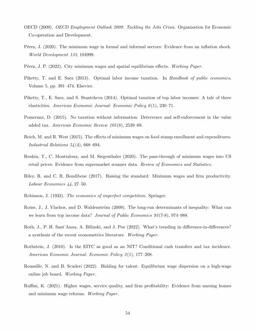
OECD (2009). OECD Employment Outlook 2009: Tackling the Jobs Crisis. Organisation for Economic

Co-operation and Development.

Perez, J. (2020). The minimum wage in formal and informal sectors: Evidence from an inflation shock.

World Development 133, 104999.

Perez, J. P. (2022). City minimum wages and spatial equilibrium effects. Working Paper .

Piketty, T. and E. Saez (2013). Optimal labor income taxation. In Handbook of public economics,

Volume 5, pp. 391–474. Elsevier.

Piketty, T., E. Saez, and S. Stantcheva (2014). Optimal taxation of top labor incomes: A tale of three

elasticities. American Economic Journal: Economic Policy 6 (1), 230–71.

Pomeranz, D. (2015). No taxation without information: Deterrence and self-enforcement in the value

added tax. American Economic Review 105 (8), 2539–69.

Reich, M. and R. West (2015). The effects of minimum wages on food stamp enrollment and expenditures.

Industrial Relations 54 (4), 668–694.

Renkin, T., C. Montialoux, and M. Siegenthaler (2020). The pass-through of minimum wages into US

retail prices: Evidence from supermarket scanner data. Review of Economics and Statistics.

Riley, R. and C. R. Bondibene (2017). Raising the standard: Minimum wages and firm productivity.

Labour Economics 44, 27–50.

Robinson, J. (1933). The economics of imperfect competition. Springer.

Roine, J., J. Vlachos, and D. Waldenstrom (2009). The long-run determinants of inequality: What can

we learn from top income data? Journal of Public Economics 93 (7-8), 974–988.

Roth, J., P. H. Sant’Anna, A. Bilinski, and J. Poe (2022). What’s trending in difference-in-differences?

a synthesis of the recent econometrics literature. Working Paper .

Rothstein, J. (2010). Is the EITC as good as an NIT? Conditional cash transfers and tax incidence.

American Economic Journal: Economic Policy 2 (1), 177–208.

Roussille, N. and B. Scuderi (2022). Bidding for talent: Equilibrium wage dispersion on a high-wage

online job board. Working Paper .

Ruffini, K. (2021). Higher wages, service quality, and firm profitability: Evidence from nursing homes

and minimum wage reforms. Working Paper .

54

Saez, E. (2001). Using elasticities to derive optimal income tax rates. The Review of Economic Stud-

ies 68 (1), 205–229.

Saez, E. (2002). Optimal income transfer programs: Intensive versus extensive labor supply responses.

The Quarterly Journal of Economics 117 (3), 1039–1073.

Saez, E. (2021). Public economics and inequality: Uncovering our social nature. AEA Papers and

Proceedings 111, 1–26.

Saez, E. and S. Stantcheva (2016). Generalized social marginal welfare weights for optimal tax theory.

The American Economic Review 106 (1), 24–45.

Saez, E. and G. Zucman (2021). Increasing the minimum wage through tax policy. Working Paper .

Savage, L. J. (1954). The foundations of statistics. John Wiley, New York, NY.

Shapiro, C. and J. E. Stiglitz (1984). Equilibrium unemployment as a worker discipline device. The

American Economic Review 74 (3), 433–444.

Shi, S. (2009). Directed search for equilibrium wage–tenure contracts. Econometrica 77 (2), 561–584.

Simon, A. and M. Wilson (2021). Optimal minimum wage setting in a federal system. Journal of Urban

Economics 123, 103336.

Sleet, C. and H. Yazici (2017). Taxation, redistribution and frictional labor supply. Working Paper .

Slemrod, J. and S. Yitzhaki (2002). Tax avoidance, evasion, and administration. In Handbook of Public

Economics, Volume 3, pp. 1423–1470. Elsevier.

Sockin, J. (2021). Show me the amenity: Are higher-paying firms better all around? Working Paper .

Sokolova, A. and T. Sorensen (2021). Monopsony in labor markets: A meta-analysis. ILR Review 74 (1),

27–55.

Sorkin, I. (2015). Are there long-run effects of the minimum wage? Review of Economic Dynamics 18 (2),

306–333.

Sorkin, I. (2018). Ranking firms using revealed preference. The Quarterly Journal of Economics 133 (3),

1331–1393.

Staiger, D. O., J. Spetz, and C. S. Phibbs (2010). Is there monopsony in the labor market? Evidence

from a natural experiment. Journal of Labor Economics 28 (2), 211–236.

Stantcheva, S. (2014). Optimal income taxation with adverse selection in the labour market. The Review

of Economic Studies 81 (3), 1296–1329.

55

Stigler, G. J. (1946). The economics of minimum wage legislation. The American Economic Review 36 (3),

358–365.

Taber, C. and R. Vejlin (2020). Estimation of a roy/search/compensating differential model of the labor

market. Econometrica 88 (3), 1031–1069.

Vaghul, K. and B. Zipperer (2016). Historical state and sub-state minimum wage data. Washington

Center for Equitable Growth.

Vergara, D. (2022). Do policies and institutions matter for pre-tax income inequality? Cross-country

evidence. International Tax and Public Finance 29 (1), 30–52.

Wolthoff, R. (2018). Applications and interviews: Firms’ recruiting decisions in a frictional labour market.

The Review of Economic Studies 85 (2), 1314–1351.

Wright, R., P. Kircher, B. Julien, and V. Guerrieri (2021). Directed search and competitive search: A

guided tour. Journal of Economic Literature 59 (1), 90–148.

Wu, L. (2021). Partially directed search in the labor market. Working Paper .

Zucman, G. (2014). Taxing across borders: Tracking personal wealth and corporate profits. Journal of

Economic Perspectives 28 (4), 121–48.

56

Minimum Wages and Optimal Redistribution

in the Presence of Taxes and Transfers

Online Appendix

Damian Vergara - UC Berkeley1

A Additional theoretical results i

B Proofs vii

C Additional figures and tables x

D Details of the calibration of Proposition II xviii

1Email: damianvergara@berkeley.edu.

A Additional theoretical results

Firm’s problem The first-order conditions of a firm of type ψ are given by

ws : (ψ · φs − ws) · qsw = qs, (A.I)

vs : (ψ · φs − ws) · qs = ηsv, (A.II)

for s ∈ {l, h}, where φs = ∂φ/∂ns and arguments are omitted from functions to simplify notation. Is

direct from the FOCs that wages are below the marginal productivities, that is, that ψ · φs > ws. Also,

combining both FOCs yields qs2 = ηsv · qsw. Differentiating and rearranging terms yields

dws

dvs=

ηsvv · qsw2qs · qsw − ηsv · qsww

> 0, (A.III)

provided qsww < 0.2 Moreover, differentiating (A.II) yields

(dψ · φs + ψ · dφs − dws) · qs + (ψ · φs − ws) · qsw · dws = ηsvv · dvs. (A.IV)

Note that

dφs = φss · (qsw · dws · vs + qs · dvs) + φsj ·(qjw · dwj · vj + qj · dvj

), (A.V)

where j is the other skill-type. Replacing (A.I) and (A.V) in (A.IV), yields

(dψ · φs + ψ ·

[φss · (qsw · dws · vs + qs · dvs) + φsj ·

(qjw · dwj · vj + qj · dvj

)])· qs = ηsvv · dvs. (A.VI)

2Ignoring the superscripts, note that qw = qθ · (∂θ/∂w), which is positive in equilibrium since U is fixed. Then

qww = qθθ ·(∂θ

∂w

)2

+ qθ ·∂2θ

∂w2.

In principle the sign of qww is ambiguous, since qθθ > 0 and ∂2θ/∂w2 > 0. I assume that the second term dominates

so qww < 0. If M(L, V ) = LδV 1−δ, sgn [qww] = sgn[−(1−T ′(w))2

1−δ − T ′′(w)], so the condition holds as long as the tax

system is not too concave. In any case, for the result above, qww < 0 is a sufficient but not necessary condition, thatis, qww is allowed to be moderately positive, which is plausible since the opposite forces in qww are interrelated. qθθ > 0follows the concavity and constant returns to scale of the matching function. To see why ∂2θ/∂w2 > 0, recall that dU =pθ · dθm · (wm − T (wm)− y0) + pm · (1− T ′(w)) · dwm. Setting dU = 0 and differentiating again yields

0 =

(ym · pθθ ·

∂θm∂wm

+ 2 · pθ · (1− T ′(wm))

)· ∂θm∂wm

+ pθ · ym ·∂2θm∂w2

m

− pm · T ′′(wm),

which implies that ∂2θ/∂w2 > 0 as long as the tax system is not too concave.

i

Setting dψ = 0 and rearranging terms gives

dvs

dvj=

[φsj ·

(qjw ·

dwj

dvj· vj + qj

)]−1

·[ηsvvψ · qs

− φss ·(qsw ·

dws

dvs· vs + qs

)], (A.VII)

which, given (A.III), implies that sgn (dvs/dvj) = sgnφsj . Also, departing from (A.VI), I can write

dws

dψ= φs ·

[ηsvvqs· dv

s

dws− ψ ·

(φss ·

(qs · vs + qs · dv

s

dws

)+

φsj ·dvj

dvs· dv

s

dws·(qjw ·

dwj

dvj· vj + qj

))]−1

. (A.VIII)

Note that dws/dψ is positive provided the cross effects do not dominate.

Firms’ responses to changes in the minimum wage To see the effect of the minimum wage on

firms’ decisions, note that the four first order conditions (equations (A.I) and (A.II) for s = {l, h}) hold

for firms that are not constrained by the minimum wage, while (A.I) no longer holds for firms that are

constrained by the minimum wage. Then, for firms that operate in sub-markets with wlm > w, it is

sufficient to verify the reaction of one of the four endogenous variables to changes in the minimum wage

and use the within-firm correlations to predict reactions in the other variables. For firms that operate

in sub-markets that wlm = w, it is necessary to first compute the change in low-skill vacancies and then

infer the changes in high-skill vacancies and wages using the within-firm between-skill correlations that

still hold for the firm.

In both cases, it is easier to work with equation (A.II) for s = l. For an unconstrained firm, totally

differentiating the first order condition and setting dψ = 0 yields

(ψ ·[φll ·

(qlθ · dθl · vl + ql · dvl

)+ φlh ·

(qhθ · dθh · vh + qh · dvh

)]− dwl

)· ql

+(ψ · φl − wl) · qlθ · dθl = ηlvv · dvl,

where I omitted sub-market sub-indices to simplify notation. Rearranging terms gives

dwl ·[dvl

dwl·(ηlvv − ψ · φll · ql2 − ψ · φlh · qh · ql ·

dvh

dvl

)+ ql

]= dθl · qlθ ·

[(ψ · φl − wl) + ψ · φll · vl · ql

]+ dθh · qhθ · φlh · ql. (A.IX)

Note that the sign and magnitude of dwl/dw is ambiguous but is likely to be non-zero since it depends

on dθl/dw. With the variation in wages it is possible to predict variation in vacancies (and, therefore,

firm-size) and spillovers to high-skill workers.

On the other hand, for a constrained firm, totally differentiating the first order condition and setting

ii

dψ = 0 yields

(ψ ·[φll ·

(qlθ · dθl · vl + ql · dvl

)+ φlh ·

(qhθ · dθh · vh + qh · dvh

)]− dw

)· ql

+(ψ · φl − w) · qlθ · dθl = ηlvv · dvl,

where I omitted sub-market sub-indices to simplify notation. Rearranging terms gives

dvl

dw·(ηlvv − ψ · φll · ql2 − ψ · φlh · qh · ql ·

dvh

dvl

)=

dθl

dw· qlθ ·

[(ψ · φl − w) + ψ · φll · vl · ql

]+dθh

dw· qhθ · φlh · ql − ql. (A.X)

Again, the sign is ambiguous but depends on the reaction on equilibrium sub-market tightness. However,

note that the first-order effect is decreasing in productivity, since (ψ · φl − w)→ 0 as w increases. That

is, among firms that pay the minimum wage, the least productive ones are more likely to decrease their

vacancies, and therefore shrink and eventually close.

Finally, to see the effect of the minimum wage on profits, we can use the envelope theorem and

conclude that the total effect is equal to the partial effect ignoring general equilibrium changes. For an

unconstrained firm, the first-order effects on profits of changes in the minimum wage are negligible. For

constrained firms there is an increase in labor costs and a mechanic increase in job-filling probabilities.

Formally

dΠ(ψ)

dw=∂Π(ψ)

∂w= qlθ ·

∂θl

∂wl· vl · (ψ · φl − w)− vl · ql. (A.XI)

This effect is negative given that the first-order condition with respect to low-skill wages holds with

inequality and is stronger for less productive firms.

Employment effects and workers’ welfare For simplicity, assume away taxes. Recall that, in equi-

librium, U s = psm · wsm. Multiplying by Lsm at both sides and integrating over m yields LsA · U s =∫Esmw

smdm, where Esm = Lsm · psm is the mass of employed workers of skill s in sub-market m. Differen-

tiating gives

dU s

dw· (LsA + U s · αs · fs(U s)) =

∫ (dEsmdw· wsm + Em ·

dwsmdw

)dm, (A.XII)

where I used LsA = αs · Fs(U s). The left-hand side is the welfare effect on workers times a positive

expression. Then, the right-hand side can be used to calculate the wage-weighted disemployment effects,∫(dEsm/dw)wsmdm, that can be tolerated for the minimum wage to still increase aggregate welfare for

workers given positive wage effects. Note that if both employment and wage effects are positive, the

iii

welfare effect on workers has to be positive (possibly attenuated by a participation response).

Average welfare weight of capitalists under optimal taxes Consider (B.IX). The FOC w.r.t. t

is given by

∂L∂t

=∂KI

∂t·G(y0)−K · ∂ψ

∗

∂t·G(y0) · o(ψ∗)−K ·

∫ ψ

ψ∗G′((1− t)Π(ψ)− ξ)Π(ψ)dO(ψ)

+γ ·K ·∫ ψ

ψ∗Π(ψ)dO(ψ)− t ·K · ∂ψ

∗

∂t·Π(ψ∗) · o(ψ∗)− y0 ·

∂KI

∂t= 0. (A.XIII)

The first two terms cancel out. Then, the expression can be rewritten as

γ ·K ·∫ ψ

ψ∗(1− gψ) Π(ψ)dO(ψ) =

∂KI

∂t(tΠ(ψ∗) + y0) . (A.XIV)

The right-hand-side is negative, which implies that

∫ ψ

ψ∗gψωψdO(ψ) < 1, (A.XV)

where ωψ = Π(ψ)/∫ ψψ∗ Π(ψ)dO(ψ) is a profit-based weight.

Additional discussion on the limitations of the model I briefly discuss the implications of ab-

stracting from dynamics, intensive margin responses, capital in the production function, and informal

labor markets.

Dynamics: The model is static. The implications of this assumption for the optimal policy analysis

are, in principle, ambiguous. Dube et al. (2016) and Gittings and Schmutte (2016) show that minimum

wage shocks decrease employment flows –separation, hires, and turnover rates– while keeping the em-

ployment stock constant, thus increasing job stability. In the presence of labor market frictions, this

induces a dynamic efficiency gain from minimum wage increases that is not captured by the model. On

the other hand, Sorkin (2015), Aaronson et al. (2018), and Hurst et al. (2022) argue that the long-run

employment distortions of minimum wage shocks are larger than the short-run responses, thus reducing

the attractiveness of the minimum wage policy. This is driven by long-run capital substitution that is

also absent from the model (see below).

Intensive margin responses: The model assumes segmented labor markets. This assumption implies

that the model abstracts from intensive margin responses (Saez, 2002). For example, increasing the

minimum wage could induce high-skill workers to apply to low-skill vacancies. To the extent that these

responses are empirically relevant, this is a caveat of the policy analysis. Note that this is different from

changes in demand for skills, as suggested by Butschek (2022) and Clemens et al. (2021). The model can

iv

rationalize this by changes in the skill composition of posted vacancies mediated by φ. Intensive margin

responses could also affect incentives conditional on labor market segmentation. For example, workers

may want to work more hours if the after-tax wage increases. This mechanism is muted in the model,

mainly motivated by the fact that at the bottom of the wage distribution extensive margin responses tend

to play a more important role to understand workers behavior. The empirical analysis finds no effect on

hours worked conditional on employment, providing empirical support to the assumption.

Capital in the production function: The production function is only a function of labor. However,

firms may also use capital. This is a caveat of the policy analysis since minimum-wages could in principle

induce capital-labor substitution in the long-run (Sorkin, 2015; Hurst et al., 2022). However, Harasztosi

and Lindner (2019) finds that firms that pay the minimum wage are usually labor intensive, which is

consistent with the estimated heterogeneities in the estimated profit elasticities. Therefore, even if capital-

labor substitution is substantive, it is unlikely to have a meaningful impact on aggregate outcomes. This

point is also related to the discussion on the labor market effects of automation (e.g., Autor, 2015;

Acemoglu and Restrepo, 2019) since minimum wage shocks could accelerate labor-saving automation.

While evidence in this regard is scarce, Ashenfelter and Jurajda (2022) study of McDonald’s restaurants

suggests that minimum wage shocks have not accelerated the automation process. They show that the

differential adoption of touch screen ordering technology across franchises is not correlated with local

minimum wage increases.

Informality : In some contexts, the interaction between the minimum wage and the degree of formality

of the labor market may be a first order consideration. In the model, the costs of participating in the

labor market, which are not taxed, may rationalize heterogeneity in outside options, including informal

labor market opportunities. However, changing the characteristics of the formal sector may affect both

the supply and demand for formal jobs. For detailed analyses, see Bosch and Manacorda (2010), Meghir

et al. (2015), Perez (2020), and Haanwinckel and Soares (2021).

Additional discussion on the empirical effects of minimum wages I briefly discuss the price

and productivity effects found in the empirical literature and its implications from abstracting from them

in the optimal policy analysis.

Price effects: The model assumes that output prices are fixed, ruling out price increases driven

by minimum wage shocks. However, the empirical literature finds substantial passthrough to prices

(Allegretto and Reich, 2018; Harasztosi and Lindner, 2019; Renkin et al., 2020; Ashenfelter and Jurajda,

2022; Leung, 2021). Modeling price increases after minimum wage shocks in the presence of limited

employment effects is challenging: if employment does not fall and demand curves are downward sloping,

prices should decrease rather than increase. Bhaskar and To (1999) and Sorkin (2015) try to formally

reconcile limited employment effects with price increases. Price effects matter for welfare since they can

v

erode nominal minimum wage increases. Also, the unemployed and non-employed households can be

made worse off given the absence of nominal improvements (MaCurdy, 2015). The distributional effect

depends on which consumers buy the goods produced by firms that pay the minimum wage, and the

relative importance of these goods in consumption bundles. It also depends on the share of minimum

wage workers since it affects the mapping from product-level prices to economy-level price indexes.

While more research is needed to assess the distributional impacts of the price effects, the available

evidence suggests that they are unlikely to play a big role in the aggregate distributional analysis. Min-

imum wage workers represent a small share of the aggregate labor market, so it is unlikely that a small

share of price increases can have substantial effects on aggregate price indexes. Also, Harasztosi and

Lindner (2019) show that the goods produced by firms that pay the minimum wage are evenly con-

sumed across the income distribution, which neutralizes the potential unintended consequences through

redistribution from high-income consumers to low-skill workers. Ashenfelter and Jurajda (2022) analyze

McDonald’s restaurants responses to local minimum wage shocks and show that the elasticity of the

number of Big Mac’s that can be purchased by minimum wage workers is around 80% of the own-wage

elasticity, meaning that even if workers spend all their money in Big Mac’s, their real wage increases are

still sizable. Renkin et al. (2020) also suggest that the price effects do not neutralize the redistributive

potential of the minimum wage, arguing that: “the rise in grocery store prices following a $1 minimum

wage increase reduces real income by about $19 a year for households earning less than $10,000 a year.

(...). The price increases in grocery stores offset only a relatively small part of the gains of minimum wage

hikes. Minimum wage policies thus remain a redistributive tool even after accounting for price effects in

grocery stores.” Based on these pieces of evidence, I conjecture that ignoring price effects is unlikely to

dramatically affect the conclusions of the policy analysis.

Productivity effects: The model assumes that technology and labor productivity are independent from

the minimum wage. This abstracts from recent literature that finds that minimum wages can increase both

workers’ (Ku, 2022; Coviello et al., 2021; Ruffini, 2021) and firms’ (Riley and Bondibene, 2017; Mayneris

et al., 2018) productivities. Potential mechanisms include efficiency wages (Shapiro and Stiglitz, 1984)

and effects on investment in training (Acemoglu and Pischke, 1999). Harasztosi and Lindner (2019) argue

that it is unlikely that productivity increases play a major role at the firm level as it would contradict

the heterogeneous employment effects found between tradable and non-tradable sectors. If these effects

are substantial, abstracting from these worker- and firm-specific increases in productivity after minimum

wage hikes is likely to make the case for a positive minimum wage conservative. Note, however, that the

model can accommodate aggregate increases in productivity through reallocation effects, as in Dustmann

et al. (2022). Importantly, the main policy results depend on reduced-form profit elasticities that are

robust to productivity increases.

vi

B Proofs

Proof of Proposition I In the absence of taxes, there is no budget constraint and the social welfare

function is given by

SW (w) =(LlI + LhI +KI

)·G(0) + αl ·

∫ U l

0G(U l − c)dFl(c)

+αh ·∫ Uh

0G(Uh − c)dFh(c) +K ·

∫ ψ

ψ∗G (Π(ψ)− ξ) dO(ψ). (B.I)

Replacing LlI + LhI = 1− LlA − LhA, the total derivative with respect to the minimum wage is given by

dSW

dw=

(dKI

dw−dLlAdw−dLhAdw

)·G(0)

+αl ·G(0) · fl(U l) ·dU l

dw+ αl ·

dU l

dw·∫ U l

0G′(U l − c)dFl(c)

+αh ·G(0) · fh(Uh) · dUh

dw+ αh ·

dUh

dw·∫ Uh

0G′(Uh − c)dFh(c)

+K ·

(∫ ψ

ψ∗G′(Π(ψ)− ξ)dΠ(ψ)

dwdO(ψ)− dψ∗

dw·G(0) · o(ψ∗)

). (B.II)

Note that dLsA/dw = d(αs · Fs(U s))/dw = αs · fs(U s) · (dU s/dw), for s ∈ {l, h}, and that dKI/dw =

d(K ·O(ψ∗))/dw = K · o(ψ∗) · (dψ∗/dw). Then, (B.II) is reduced to

dSW

dw= αs ·

dU l

dw·∫ U l

0G′(U l − c)dFl(c) + αh ·

dUh

dw·∫ Uh

0G′(Uh − c)dFh(c)

+K ·∫ ψ

ψ∗G′(Π(ψ)− ξ)dΠ(ψ)

dwdO(ψ). (B.III)

Using the marginal welfare weights definitions, (B.III) is reduced to

dSW

dw= γ ·

(dU l

dw· LlA · gl1 +

dUh

dw· LhA · gh1 +K ·

∫ ψ

ψ∗gψdΠ(ψ)

dwdO(ψ)

). (B.IV)

vii

Proof of Proposition II The Lagrangian is given by

L(w, y0) =(LlI + LhI +KI

)·G(y0)

+αl ·∫ U l−y0

0G(U l − c)dFl(c) + αh ·

∫ Uh−y0

0G(Uh − c)dFh(c)

+K ·∫ ψ

ψ∗G((1− t)Π(ψ)− ξ)dO(ψ) + γ ·

[∫ (ElmT (wlm) + EhmT (whm)

)dm

+t ·K ·∫ ψ

ψ∗Π(ψ)dO(ψ)− y0

(LlI + LhI +KI + ρl · LlA + ρh · LhA

)], (B.V)

where γ is the budget constraint multiplier. Since ρs · LsA = LsA −∫Esmdm, and the fact that LlI + LhI +

LlA + LhA = 1, the expression is simplified to

L(w, y0) =(LlI + LhI +KI

)·G(y0)

+αl ·∫ U l−y0

0G(U l − c)dFl(c) + αh ·

∫ Uh−y0

0G(Uh − c)dFh(c)

+K ·∫ ψ

ψ∗G((1− t)Π(ψ)− ξ)dO(ψ) + γ ·

[∫ (Elm(T (wlm) + y0)

+Ehm(T (whm) + y0))dm+ t ·K ·

∫ ψ

ψ∗Π(ψ)dO(ψ)− y0 (1 +KI)

]. (B.VI)

The derivative with respect to w, taking y0, t, and T (·) as given, is given by

dLdw

=

(dKI

dw−dLsAdw−dLhAw

)·G(y0)

+G(y0) · αl · fl(U l − y0) · dUl

dw+ αl ·

dU l

dw·∫ U l−y0

0G′(U l − c)dFl(c)

+G(y0) · αh · fh(Uh − y0) · dUh

dw+ αh ·

dUh

dw·∫ Uh−y0

0G′(Uh − c)dFh(c)

+K ·

[∫ ψ

ψ∗G′((1− t)Π(ψ)− ξ)(1− t)dΠ(ψ)

dwdO(ψ)−G(y0) · o(ψ∗) · dψ

∗

dw

]

γ ·[∫ (

dElmdw

(T (wlm) + y0

)+ ElmT

′(wlm)dwlmdw

+dEhmdw

(T (whm) + y0

)+ EhmT

′(whm)dwhmdw

)dm

+t ·K ·

(∫ ψ

ψ∗

dΠ(ψ)

dwdO(ψ)−Π(ψ∗) · o(ψ∗) · dψ

∗

dw

)− y0 ·

dKI

dw

]. (B.VII)

Recall that dKI/dw = K · o(ψ∗) · (dψ∗/dw) and dLsA/dw = αs · fs(U s − y0) · (dU s/dw) for s ∈ {l, h}.

viii

Using the social marginal weights definitions, and grouping common terms, (B.VII) can be written as

dLdw· 1

γ=

dU l

dw· LlA · gl1 +

dUh

dw· LhA · gh1 +K · (1− t) ·

∫ ψ

ψ∗gψdΠ(ψ)

dwdO(ψ)

+

∫ (dElmdw

(T (wlm) + y0

)+ ElmT

′(wlm)dwlmdw

)dm

+

∫ (dEhmdw

(T (whm) + y0

)+ EhmT

′(whm)dwhmdw

)dm

+t ·K ·∫ ψ

ψ∗

dΠ(ψ)

dwdO(ψ)− dKI

dw· (t ·Π(ψ∗) + y0) . (B.VIII)

Proof of Proposition III I assume that the planner optimizes allocations instead of taxes. That is,

the planner chooses ∆ysm = ysm − y0, for all m and s ∈ {l, h}, and then recover taxes by noting that

T (wsm) + y0 = wsm −∆ysm. This implies that the Lagrangian is given by

L (w, {∆ysm}, y0) =(LlI + LhI +KI

)·G(y0)

+αl ·∫ U l−y0

0G(U l − c)dFl(c) + αh ·

∫ Uh−y0

0G(Uh − c)dFh(c)

+K ·∫ ψ

ψ∗G((1− t)Π(ψ)− ξ)dO(ψ)

+γ ·[∫ (

Elm(wlm −∆ylm) + Ehm(whm −∆yhm))dm

+t ·K ·∫ ψ

ψ∗Π(ψ)dO(ψ)− y0 (1 +KI)

]. (B.IX)

There are two differences w.r.t. to the first-order condition derived for Proposition II. First, now the

planner takes partial derivatives rather than total derivatives, leaving ∆ysm constant, for all m and s ∈

{l, h} when choosing the minimum wage. This implies that the relevant elasticities are micro rather than

macro elasticities. Second, this transformation affects the term in the budget constraint that previously

contained T (·). This implies that the optimality condition of the minimum wage can be written as

∂L∂w· 1

γ=

∂U l

∂w· LlA · gl1 +

∂Uh

∂w· LhA · gh1 +K · (1− t) ·

∫ ψ

ψ∗gψ∂Π(ψ)

∂wdO(ψ)

+

∫ (∂Elm∂w

(T (wlm) + y0

)+ Elm

∂wlm∂w

)dm

+

∫ (∂Ehm∂w

(T (whm) + y0

)+ Ehm

∂whm∂w

)dm

+t ·K ·∫ ψ

ψ∗

∂Π(ψ)

∂wdO(ψ)− ∂KI

∂w· (t ·Π(ψ∗) + y0) . (B.X)

See the main text for a discussion on micro versus macro elasticities.

ix

C Additional figures and tables

Table C.I: List of Events

State Events (in bold the selected sample) Total

Alabama - 0Alaska 2003, 2015, 2016 3Arizona 2007, 2009, 2012, 2017, 2018, 2019 6Arkansas 2006, 2015, 2016, 2017, 2019 5California 1988, 1997, 1998, 2001, 2002, 2007, 2008, 2014, 2016, 2017, 2018, 2019 12Colorado 2007, 2009, 2015, 2017, 2018, 2019 6

Connecticut 1980, 1981, 1988, 1999, 2009, 2015, 2016, 2017 8Delaware 2000, 2007, 2014, 2015, 2019 5

District of Columbia 1980, 1987, 1993, 2014, 2015, 2016, 2017, 2018 8Florida 2005, 2009, 2012 3Georgia - 0Hawaii 1988, 1993, 2002, 2003, 2006, 2007, 2015, 2016, 2017, 2018 10Idaho - 0Illinois 2005, 2007, 2010 3Indiana - 0

Iowa 1990, 1991, 1992, 2008 4Kansas - 0

Kentucky - 0Louisiana - 0

Maine 2017, 2018, 2019 3Maryland 2015 1

Massachusetts 1997, 2001, 2007, 2015, 2016, 2017, 2019 7Michigan 2006, 2014, 2016, 2017 4Minnesota 1988, 1989, 1991, 2014, 2015, 2016 6Mississippi - 0Missouri 2007, 2009, 2019 3Montana 2007, 2009, 2012 3Nebraska 2015, 2016 2Nevada 2006, 2009, 2010 3

New Hampshire - 0New Jersey 1992, 2006, 2014, 2019 4New Mexico 2008, 2009 2New York 2005, 2006, 2013, 2014, 2015, 2016, 2017, 2018, 2019 9

North Carolina 2007 1North Dakota - 0

Ohio 2007, 2009, 2012 3Oklahoma - 0

Oregon 1989, 1990, 1991, 1997, 1998, 1999, 2003, 2006, 2007, 2009, 2016, 2017, 2019 13Pennsylvania 1989, 2007 2Rhode Island 1986, 1989, 1999, 2000, 2006, 2015, 2016, 2019 8

South Carolina - 0South Dakota 2015 1

Tennessee - 0Texas - 0Utah - 0

Vermont 1999, 2001, 2009, 2015, 2016, 2017, 2018 7Washington 1989, 1990, 1994, 1999, 2000, 2007, 2009, 2012, 2017, 2018, 2019 11

West Virginia 2006, 2007, 2015, 2016 4Wisconsin 1989, 2006 2Wyoming - 0

x

Figure C.I: State-level real minimum wage increase by event

-.05

0

.05

.1

.15

.2

Log(

Min

imum

Wag

e)

-3 -2 -1 0 1 2 3 4Years from MW increase

Year FE Year x CR FE

(a) All events

-.05

0

.05

.1

.15

.2

Log(

Min

imum

Wag

e)

-3 -2 -1 0 1 2 3 4Years from MW increase

Year FE Year x CR FE

(b) Selected events

Notes: These figures plot the estimated βτ coefficients with their corresponding 90% confidence intervals from equation (17) using thelog of the real hourly state-level minimum wage as a dependent variable. Red lines represent specifications that control by year-by-eventfixed effects. Blue lines represent specifications that control by census-region-by-year-by-event fixed effects. Panel (a) considers all 172events. Panel (b) considers a selected sample of 72 events where treated states do not experience other events in the three years previousto the event and whose timing allow to observe the outcomes from three years before to four years after. Minimum wage data is takenfrom Vaghul and Zipperer (2016). Standard errors are clustered at the state level, and regressions are weighted by state-by-year averagepopulation computed using the CPS monthly files.

xi

Figure C.II: Changes in workers’ welfare after minimum wage increases (all events)

-.025

0

.025

.05

Log(

Aver

age

wag

e am

ong

parti

cipa

nts)

-3 -2 -1 0 1 2 3 4Years from MW increase

Year FE Year x CR FE

(a) Low-skill workers

-.025

0

.025

.05

Log(

Aver

age

wag

e am

ong

parti

cipa

nts)

-3 -2 -1 0 1 2 3 4Years from MW increase

Year FE Year x CR FE

(b) High-skill workers

-.1

-.075

-.05

-.025

0

.025

.05

Log(

Inco

me

assi

stan

ce tr

ansf

ers)

-3 -2 -1 0 1 2 3 4Years from MW increase

Year FE Year x CR FE

(c) Income maintenance benefits (total)

-.1

-.075

-.05

-.025

0

.025

.05

Log(

Inco

me

assi

stan

ce tr

ansf

ers

per w

orki

ng-a

ge p

op.)

-3 -2 -1 0 1 2 3 4Years from MW increase

Year FE Year x CR FE

(d) Income maintenance benefits (per working-age pop.)

Notes: These figures plot the estimated βτ coefficients with their corresponding 90% confidence intervals from equation (17). Estimationsconsider all 172 events. Panel (a) uses the average pre-tax wage of low-skill workers including the unemployed as dependent variable.Panel (b) uses the average pre-tax wage of high-skill workers including the unemployed as dependent variable. Panels (c) and (d) usetotal and per working-age population income maintenance benefits as dependent variable, respectively. Red lines represent specificationsthat control by year-by-event fixed effects. Blue lines represent specifications that control by census-region-by-year-by-event fixed effects.Standard errors are clustered at the state level, and regressions are weighted by state-by-year average population computed using theCPS monthly files.

xii

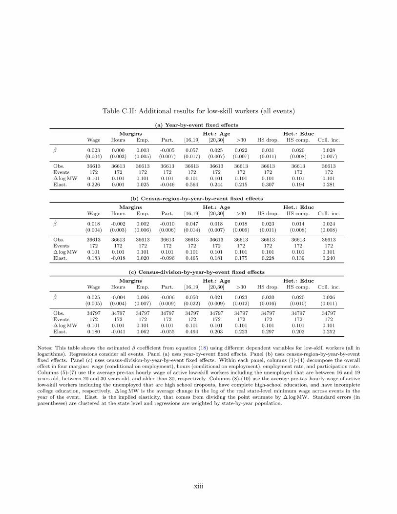
Table C.II: Additional results for low-skill workers (all events)

(a) Year-by-event fixed effects

Margins Het.: Age Het.: EducWage Hours Emp. Part. [16,19] [20,30] >30 HS drop. HS comp. Coll. inc.

β 0.023 0.000 0.003 -0.005 0.057 0.025 0.022 0.031 0.020 0.028(0.004) (0.003) (0.005) (0.007) (0.017) (0.007) (0.007) (0.011) (0.008) (0.007)

Obs. 36613 36613 36613 36613 36613 36613 36613 36613 36613 36613Events 172 172 172 172 172 172 172 172 172 172∆ log MW 0.101 0.101 0.101 0.101 0.101 0.101 0.101 0.101 0.101 0.101Elast. 0.226 0.001 0.025 -0.046 0.564 0.244 0.215 0.307 0.194 0.281

(b) Census-region-by-year-by-event fixed effects

Margins Het.: Age Het.: EducWage Hours Emp. Part. [16,19] [20,30] >30 HS drop. HS comp. Coll. inc.

β 0.018 -0.002 0.002 -0.010 0.047 0.018 0.018 0.023 0.014 0.024(0.004) (0.003) (0.006) (0.006) (0.014) (0.007) (0.009) (0.011) (0.008) (0.008)

Obs. 36613 36613 36613 36613 36613 36613 36613 36613 36613 36613Events 172 172 172 172 172 172 172 172 172 172∆ log MW 0.101 0.101 0.101 0.101 0.101 0.101 0.101 0.101 0.101 0.101Elast. 0.183 -0.018 0.020 -0.096 0.465 0.181 0.175 0.228 0.139 0.240

(c) Census-division-by-year-by-event fixed effects

Margins Het.: Age Het.: EducWage Hours Emp. Part. [16,19] [20,30] >30 HS drop. HS comp. Coll. inc.

β 0.025 -0.004 0.006 -0.006 0.050 0.021 0.023 0.030 0.020 0.026(0.005) (0.004) (0.007) (0.009) (0.022) (0.009) (0.012) (0.016) (0.010) (0.011)

Obs. 34797 34797 34797 34797 34797 34797 34797 34797 34797 34797Events 172 172 172 172 172 172 172 172 172 172∆ log MW 0.101 0.101 0.101 0.101 0.101 0.101 0.101 0.101 0.101 0.101Elast. 0.180 -0.041 0.062 -0.055 0.494 0.203 0.223 0.297 0.202 0.252

Notes: This table shows the estimated β coefficient from equation (18) using different dependent variables for low-skill workers (all inlogarithms). Regressions consider all events. Panel (a) uses year-by-event fixed effects. Panel (b) uses census-region-by-year-by-eventfixed effects. Panel (c) uses census-division-by-year-by-event fixed effects. Within each panel, columns (1)-(4) decompose the overalleffect in four margins: wage (conditional on employment), hours (conditional on employment), employment rate, and participation rate.Columns (5)-(7) use the average pre-tax hourly wage of active low-skill workers including the unemployed that are between 16 and 19years old, between 20 and 30 years old, and older than 30, respectively. Columns (8)-(10) use the average pre-tax hourly wage of activelow-skill workers including the unemployed that are high school dropouts, have complete high-school education, and have incompletecollege education, respectively. ∆ log MW is the average change in the log of the real state-level minimum wage across events in theyear of the event. Elast. is the implied elasticity, that comes from dividing the point estimate by ∆ log MW. Standard errors (inparentheses) are clustered at the state level and regressions are weighted by state-by-year population.

xiii

Figure C.III: Changes in capitalists’ welfare after minimum wage increases (all events)

-.08

-.06

-.04

-.02

0

.02

.04

.06

Log(

Aver

age

prof

it pe

r est

ablis

hmen

t)

-3 -2 -1 0 1 2 3 4Years from MW increase

Year FE Year x CR FE

(a) Profits per establishment (all industries)

-.08

-.06

-.04

-.02

0

.02

.04

.06

Log(

Aver

age

prof

it pe

r est

ablis

hmen

t)

-3 -2 -1 0 1 2 3 4Years from MW increase

Year FE Year x CR FE

(b) Profits per establishment (non-professional services)

Notes: These figures plot the estimated βτ coefficients with their corresponding 90% confidence intervals from equation (17). Estimationsconsider all 172 events. Panel (a) uses the gross operating surplus per private establishment in all industries as dependent variable.Panel (b) only considers the non-professional services industry, that is, educational services, health care, arts, entertainment, recreation,accomodation, and food services. Red lines represent specifications that control by year-by-event fixed effects. Blue lines representspecifications that control by census-region-by-year-by-event fixed effects, respectively. Standard errors are clustered at the state level,and regressions are weighted by state-by-year average population computed using the CPS monthly files.

xiv

Table C.III: Capitalists results: Industry heterogeneity

(a) Year-by-event fixed effects

All All NNRR Constr. Manuf. Transp. Wholesale Retail Finance Prof. serv Non-prof. serv.

β 0.007 0.007 0.013 -0.013 0.022 0.005 -0.018 0.010 0.005 0.019 -0.024(0.008) (0.008) (0.025) (0.031) (0.018) (0.020) (0.015) (0.010) (0.013) (0.010) (0.022)

Obs. 37749 32943 31494 32170 32098 32171 32259 32259 32259 32259 32167Events 172 157 157 157 157 157 157 157 157 157 157∆ log MW 0.101 0.099 0.100 0.099 0.099 0.099 0.099 0.099 0.099 0.099 0.099Elast. 0.068 0.072 0.132 -0.127 0.225 0.050 -0.178 0.097 0.046 0.190 -0.239

(b) Census-region-by-year-by-event fixed effects

All All NNRR Constr. Manuf. Transp. Wholesale Retail Finance Prof. serv Non-prof. serv.

β 0.006 0.004 -0.024 -0.045 0.034 -0.021 -0.021 -0.008 0.006 0.019 -0.030(0.008) (0.008) (0.025) (0.032) (0.026) (0.027) (0.017) (0.013) (0.012) (0.012) (0.010)

Obs. 37749 32943 31409 32170 32098 32171 32259 32259 32259 32259 32167Events 172 157 157 157 157 157 157 157 157 157 157∆ log MW 0.101 0.099 0.100 0.099 0.099 0.099 0.099 0.099 0.099 0.099 0.099Elast. 0.054 0.043 -0.244 -0.450 0.346 -0.214 -0.210 -0.083 0.056 0.189 -0.303

(c) Census-division-by-year-by-event fixed effects

All All NNRR Constr. Manuf. Transp. Wholesale Retail Finance Prof. serv Non-prof. serv.

β 0.008 0.006 -0.052 -0.062 0.008 -0.070 0.016 -0.012 0.000 0.008 -0.012(0.010) (0.010) (0.034) (0.036) (0.024) (0.028) (0.020) (0.010) (0.017) (0.013) (0.010)

Obs. 35914 31246 29692 30492 30423 30496 30584 30584 30584 30584 30490Events 172 157 157 157 157 157 157 157 157 157 157∆ log MW 0.102 0.099 0.100 0.099 0.099 0.099 0.099 0.099 0.099 0.099 0.099Elast. 0.076 0.065 -0.519 -0.628 0.079 -0.710 0.160 -0.124 0.002 0.081 -0.119

Notes: This table shows the estimated β coefficient from equation (18) using the gross operating surplus per private establishment fordifferent industries (all in logarithms). Panel (a) uses year-by-event fixed effects. Panel (b) uses census-region-by-year-by-event fixedeffects. Panel (c) uses census-division-by-year-by-event fixed effects. NNRR includes agriculture, forestry, fishing, hunting, and mining.Constr. includes construction. Manuf. includes durable and nondurable goods manufacturing. Transp. includes transportation.Wholesale includes wholesale trade. Retail includes retail trade. Finance includes finance, insurance, real estate, rental, and leasing.Prof. serv. includes professional and business services. Non-prof. serv. includes educational services, health care, arts, entertainment,recreation, accomodation, and food services. ∆ log MW is the average change in the log of the real state-level minimum wage acrossevents in the year of the event. Elast. is the implied elasticity, that comes from dividing the point estimate by ∆ log MW. Standarderrors (in parentheses) are clustered at the state level and regressions are weighted by state-by-year population.

xv

Figure C.IV: Changes in capitalists’ welfare after minimum wage increases: non-professional services,construction, wholesale trade, and finance

-.1

-.08

-.06

-.04

-.02

0

.02

.04

.06

Log(

Aver

age

prof

it pe

r est

ablis

hmen

t)

-3 -2 -1 0 1 2 3 4Years from MW increase

Year FE Year x CR FE

(a) Profits per establishment (all events)

-.1

-.08

-.06

-.04

-.02

0

.02

.04

.06

Log(

Aver

age

prof

it pe

r est

ablis

hmen

t)

-3 -2 -1 0 1 2 3 4Years from MW increase

Year FE Year x CR FE

(b) Profits per establishment (selected events)

Notes: These figures plot the estimated βτ coefficients with their corresponding 90% confidence intervals from equation (17). Thedependent variable is the gross operating surplus per private establishment only considering non-professional services, construction,wholesale trade, and finance. Panel (a) uses all events. Panel (b) only considers the selected sample of events. Red lines representspecifications that control by year-by-event fixed effects. Blue lines represent specifications that control by census-region-by-year-by-event fixed effects. Standard errors are clustered at the state level, and regressions are weighted by state-by-year average populationcomputed using the CPS monthly files.

xvi

Table C.IV: Additional fiscal externalities on capitalists

(a) Year-by-event fixed effects

# Estab. (All) # Estab. (All) # Estab. (Exp.) Bus. inc. Bus. inc. # of Bus. rets. Div. inc. Div. inc. # of Div. rets. S-Corp. inc. S-Corp. inc. # of S-Corp. rets.(1979-2019) (1990-2019) (1990-2019) (per ret.) (per wa pop) (per tot. ret.) (per ret.) (per wa pop) (per tot. ret.) (per ret.) (per wa pop) (per tot. ret.)

β 0.013 0.013 0.025 0.002 -0.005 -0.004 0.004 -0.003 -0.005 0.036 0.031 -0.003(0.009) (0.009) (0.011) (0.010) (0.011) (0.008) (0.020) (0.021) (0.006) (0.029) (0.027) (0.007)

Obs. 17604 17604 13732 11969 11969 11969 11969 11969 11969 5258 5258 5258Events 72 72 60 60 60 60 60 60 60 42 42 42∆MW 0.127 0.127 0.126 0.128 0.128 0.128 0.128 0.128 0.128 0.090 0.090 0.090Elast. 0.099 0.099 0.198 0.012 -0.038 -0.031 0.033 -0.026 -0.039 0.396 0.351 -0.028

(b) Census-region-by-year-by-event fixed effects

# Estab. (All) # Estab. (All) # Estab. (Exp.) Bus. inc. Bus. inc. # of Bus. rets. Div. inc. Div. inc. # of Div. rets. S-Corp. inc. S-Corp. inc. # of S-Corp. rets.(1979-2019) (1990-2019) (1990-2019) (per ret.) (per wa pop) (per tot. ret.) (per ret.) (per wa pop) (per tot. ret.) (per ret.) (per wa pop) (per tot. ret.)

β 0.007 0.007 0.016 0.006 0.006 0.002 0.002 -0.004 -0.005 0.011 0.003 -0.006(0.006) (0.006) (0.008) (0.011) (0.013) (0.006) (0.018) (0.019) (0.006) (0.027) (0.026) (0.006)

Obs. 17604 17604 13732 11969 11969 11969 11969 11969 11969 5258 5258 5258Events 72 72 60 60 60 60 60 60 60 42 42 42∆MW 0.127 0.127 0.126 0.128 0.128 0.128 0.128 0.128 0.128 0.090 0.090 0.090Elast. 0.058 0.058 0.128 0.044 0.050 0.012 0.014 -0.035 -0.043 0.118 0.029 -0.069

(c) Census-division-by-year-by-event fixed effects

# Estab. (All) # Estab. (All) # Estab. (Exp.) Bus. inc. Bus. inc. # of Bus. rets. Div. inc. Div. inc. # of Div. rets. S-Corp. inc. S-Corp. inc. # of S-Corp. rets.(1979-2019) (1990-2019) (1990-2019) (per ret.) (per wa pop) (per tot. ret.) (per ret.) (per wa pop) (per tot. ret.) (per ret.) (per wa pop) (per tot. ret.)

β 0.011 0.011 0.011 0.015 0.015 -0.002 0.030 0.023 -0.008 0.030 0.020 -0.010(0.008) (0.008) (0.007) (0.012) (0.012) (0.006) (0.012) (0.012) (0.007) (0.032) (0.030) (0.005)

Obs. 16818 16818 13069 11341 11341 11341 11341 11341 11341 4883 4883 4883Events 72 72 60 60 60 60 60 60 60 42 42 42∆MW 0.125 0.125 0.123 0.125 0.125 0.125 0.125 0.125 0.125 0.088 0.088 0.088Elast. 0.092 0.092 0.088 0.122 0.120 -0.016 0.238 0.185 -0.067 0.344 0.232 -0.111

Notes: This table shows the estimated β coefficient from equation (18) using different dependent variables (all in logarithms) usingthe selected sample of events. Regressions consider all events. Panel (a) uses year-by-event fixed effects. Panel (b) uses census-region-by-year-by-event fixed effects. Panel (c) uses census-division-by-year-by-event fixed effects. # Estab. (all) measures the number ofestablishments of all industries. # Estab. (Exp.) measures the number of establishments of non-professional services, construction,wholesale trade, and finance. The rest of the dependent variables are taken from public SOI tables at the state level. Bus. inc. isreported business income in personal tax forms, and available from 1996. Column (4) uses Bus. inc. normalized by the returns thatreport positive business income. Column (5) uses Bus. inc. normalized by working-age population. Column (6) measures the numberof returns that report positive business income. Div. inc. is reported dividend income in personal tax forms, and available from 1996.Column (7) uses Div. inc. normalized by the returns that report positive dividend income. Column (8) uses Div. inc. normalized byworking-age population. Column (9) measures the number of returns that report positive dividend income. S-Corp. inc. is reportedS-Corp income in personal tax forms, and available from 2009. Column (10) uses S-corp. inc. normalized by the returns that reportpositive business income. Column (11) uses S-corp. inc. normalized by working-age population. Column (12) measures the number ofreturns that report positive S-Corp. income. ∆ log MW is the average change in the log of the real state-level minimum wage acrossevents in the year of the event. Elast. is the implied elasticity, that comes from dividing the point estimate by ∆ log MW. Standarderrors (in parentheses) are clustered at the state level and regressions are weighted by state-by-year population.

xvii

D Details of the calibration of Proposition II

This appendix describes the details of the calibration that gives form to the results in Table 6.

Monetary values Total pre-tax earnings, total pre-tax profits, and total income maintenance transfers

are computed using the estimation sample. Total pre-tax earnings are computed using the CPS-MORG

data as described in Section 4. Since average pre-tax individual incomes are measured in hourly wages,

I multiply the annual sum of hourly wages by the average usual weekly hours worked, and 52 weeks.

Average weekly hours worked by employed low-skill workers are 32.6 and 33.7 in the cases considered

below. Total pre-tax profits per industry are directly taken from the BEA industry level estimates of

the gross operating surplus. Finally, total income maintenance benefits are taken from the BEA regional

accounts. To compute the welfare weights I also calculate average post-tax incomes of low-skill workers,

which correspond to the annualized version of the sufficient statistic (average hourly wage times average

weekly hours worked times the employment rate times 52), and average post-tax incomes of capitalists,

which correspond to the annual gross operating surplus per private establishment (taken from the QCEW

files) net of the corporate tax rate considered. Table D.I shows the computed values for the two scenarios

considered. Values are in 2016 thousand dollars. The first column is the population-weighted average

across treated states of all pre-event year observations. The second column is the population-weighted

average across states using data on year 2019. Average annual incomes of capitalists are pre-tax so post-

tax values correspond to the values of the table times (1 − t), for the different assumptions on t. While

total values are larger for workers, average incomes are several times larger for capitalists.

Table D.I: Monetary values (in 2016 thousand dollars)

Pre-event years 2019

Totals:TPTW 452,000,000 383,000,000TIMB 16,500,000 12,000,000TPTP (Non-prof. serv.) 32,800,000 30,300,000TPTP (Constr.) 13,500,000 14,100,000TPTP (Wholesale) 17,000,000 20,700,000TPTP (Finance) 170,000,000 157,000,000

Averages:Low-skill workers 17.180 20.437Cap. (Non-prof. serv.) 156.383 200.938Cap. (Constr.) 294.692 366.430Cap. (Wholesale) 499.010 711.332Cap. (Finance) 3,168.497 3,478.396

Computing εU l For each underlying model and assumption on the totals, εU l is computed as:

εU l =TPTW · ε

U l(pre-tax) + TIMB · εBTPTW + TIMB

. (D.I)

xviii

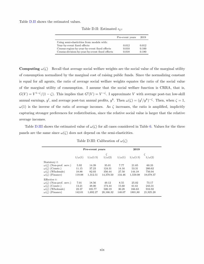
Table D.II shows the estimated values.

Table D.II: Estimated εU l

Pre-event years 2019

Using semi-elasticities from models with:Year-by-event fixed effects 0.012 0.012Census-region-by-year-by-event fixed effects 0.010 0.100Census-division-by-year-by-event fixed effects 0.018 0.180

Computing ω(ζ) Recall that average social welfare weights are the social value of the marginal utility

of consumption normalized by the marginal cost of raising public funds. Since the normalizing constant

is equal for all agents, the ratio of average social welfare weights equates the ratio of the social value

of the marginal utility of consumption. I assume that the social welfare function is CRRA, that is,

G(V ) = V 1−ζ/(1− ζ). This implies that G′(V ) = V −ζ . I approximate V with average post-tax low-skill

annual earnings, yl, and average post-tax annual profits, yk. Then ω(ζ) = (yl/yk)−ζ . Then, when ζ = 1,

ω(1) is the inverse of the ratio of average incomes. As ζ increases, the ratio is amplified, implicitly

capturing stronger preferences for redistribution, since the relative social value is larger that the relative

average incomes.

Table D.III shows the estimated value of ω(ζ) for all cases considered in Table 6. Values for the three

panels are the same since ω(ζ) does not depend on the semi-elasticities.

Table D.III: Calibration of ω(ζ)

Pre-event years 2019

ζ ζ1/ω(1) 1/ω(1.5) 1/ω(2) 1/ω(1) 1/ω(1.5) 1/ω(2)

Statutory t:ω(ζ) (Non-prof. serv.) 5.92 14.39 35.01 7.77 21.65 60.33ω(ζ) (Constr.) 11.15 37.23 124.31 14.16 53.31 200.62ω(ζ) (Wholesale) 18.88 82.03 356.44 27.50 144.18 756.04ω(ζ) (Finance) 119.88 1,312.51 14,370.50 134.46 1,559.08 18,078.37

Effective t:ω(ζ) (Non-prof. serv.) 7.01 18.56 49.12 8.55 25.02 73.17ω(ζ) (Constr.) 13.21 48.00 174.44 15.60 61.61 243.31ω(ζ) (Wholesale) 22.37 105.77 500.19 30.28 166.63 916.92ω(ζ) (Finance) 142.01 1,692.27 20,166.32 148.07 1801,80 21,925.20

xix