Sticky Wages, Profitability, and Momentum ∗

Morad Zekhnini †

November 13, 2015

∗I would like to thank Kerry Back, Jefferson Duarte, Gustavo Grullon, Yamil Kaba, BarbaraOstdiek, James Weston, Yuhang Xing, and seminar participants at Rice University.†Graduate Student, Department of Finance, Jones School of Business, Rice University, 6100

Main Street, Houston, TX, 77005; email: Morad.Zekhnini@rice.edu

Abstract

Wage stickiness and firm-specific human capital induce operating lever-

age that contributes to the risk exposure of the firm. This leverage pro-

duces momentum in returns as well as a positive relationship between prof-

its and subsequent returns. I demonstrate these relationships in the context

of a partial equilibrium production model. I empirically show that mo-

mentum and profitability returns are more pronounced in the presence of

labor-induced operating leverage. A novel implication of the model is that

recession-resistant stocks earn higher returns during subsequent expansions.

This prediction holds empirically and is distinct from other anomalies.

2

1 Introduction

The persistence of momentum profits, first documented by Jegadeesh and Titman

(1993), remains a major challenge to rational efficient market models. The recent

work of Novy-Marx (2013) documents a conceptually related regularity in equity

returns: profitable firms earn higher returns. I propose a rational explanation for

momentum and profitability returns based on cross-sectional dispersion in oper-

ating leverage that is positively correlated with past performance. The operating

leverage is due to high wages paid by profitable firms and is attributed to frictions

in the labor market. Empirically, I show that both the labor environment and

employee wages are associated with firm risk. In addition, I provide support for

a counterintuitive implication of the mechanism underlying the link between la-

bor and firm risk, namely that recession-resistant stocks are risky and earn higher

returns.

The main frictions that I consider are rigidities in wages, specifically wage

stickiness. Combined with production technologies that benefit from firm-specific

human capital, these rigidities render individual firm labor demand less elastic to

market conditions compared to a frictionless model. Intuitively, firm-specific hu-

man capital induces firms to retain employees despite the incidence of bad times,

while sticky wages discourage hiring new employees during good times. Conse-

quently, the wage bill is a source of operating leverage as it behaves like a fixed

cost as opposed to a variable cost. Labor market frictions and their financial im-

pact have been the focus of a growing body of work on the intersection of labor

and finance (e.g. Eisfeldt and Papanikoloau (2013) and Belo, Lin, and Bazdresch

(2014)). To my knowledge, this is the first paper to establish a link between labor

1

frictions and the momentum and profitability anomalies.

To model labor frictions, I consider a production economy in which output de-

pends on the tenure of the labor force. Tenure reflects firm-specific human capital

accumulated during employment. The market wage for new hires fluctuates, and

the firm must match increases to retain employees. However, the firm cannot cut

wages when the new-hire rate falls without losing workers and having to rehire

workers with lower firm-specific human capital. In reality, cutting wages can lead

to lower morale and productivity.1 I model this reluctance to reduce wages in a

simple way by assuming that the entire workforce departs if a firm cuts wages to

match the market rate. Thus, whenever the firm’s wage rate is above the market

rate, the firm has an option to cut wages at the cost of lower productivity due to

the loss of employees with firm-specific human capital. This option is exercised

only infrequently in equilibrium, and it tends to be exercised by firms with adverse

productivity shocks. As a result, more profitable firms tend to have the option in

place and therefore be more risky than less profitable firms.

To test the relationship between the labor environment and the momentum and

profitability anomalies, I hypothesize that firms lack the flexibility to lay off work-

ers in heavily unionized industries. In the absence of this option to restructure, the

cross-sectional variation in labor-induced leverage is small and the momentum and

profitability returns are likely to be small as well. Implementing the momentum

strategy in a restricted sample of heavily unionized industry firms yields a Fama-

French-Carhart monthly alpha of 0.77% compared to 1.36% in the full sample.

1Solow (1979) and Akerlof (1982) offer sociological-based explanations for wage rigiditycouched in the concept of “gift exchange,” whereby employee morale and productivity are tied towages. Bewely (1998) finds support for this explanation using survey data and Kube, Marechal,and Puppe (2013) conduct a field experiment whose results are consistent with the gift exchangetheory for wage stickiness.

2

On the other hand, the momentum strategy in low- and non-unionized industries

earns a monthly alpha of 1.84%. A similar relationship holds when I implement

the profitability strategy in the two subsamples. The profitability alpha in the

unionized-firm sample is 0.46%, nearly half the strategy’s alpha of 0.85% in the

non-union sample.

One of the salient features of the model is the role that labor wages play in

determining the risk exposure of the firm. Firm wages can therefore serve as

predictors of future returns. The model predictions are consistent with recent

findings regarding wage share (Donangelo, Gourio and Palacios (2015)). Firms or

industries where labor is a more important input into production have higher risk

exposure and hence earn higher returns. For a more direct test of the relationship

between employee compensation and firm risk I use defined benefit plan contribu-

tion data.2 Using defined benefit plan employer contributions as a proxy for the

compensation that firms pay their employees, I find that firms with relatively high

employee compensation earn a monthly factor-adjusted alpha that is 0.46% higher

than low compensation firms.

A novel prediction of a model with these frictions is that recession-resistant

stocks are risky and should command a premium. Aggregate conditions dictate

the market wage, a key factor in each firm’s decision to exercise its restructuring op-

tion. Therefore, the variation in risk exposure is more evident following aggregate

downturns, i.e. recessions, when aggregate wages drop and firms are more likely to

lay off workers. I test this prediction by constructing a measure of the cyclicality

of gross profits: the difference between recession and non-recession profits. I then

2The data on wages for U.S. firms are sparsely populated in the Compustat database (seeCrawford, Nelson and Rountree (2014)).

3

build portfolios on the basis of this measure and observe the portfolio returns. The

high-minus-low portfolio that is long less cyclical stocks and short cyclical stocks

earns a Fama-French-Carhart-adjusted monthly alpha of 0.27%. One important

feature of this measure is that it captures a low frequency phenomenon. For each

firm in my sample the measure stays constant over an entire business cycle. Cor-

respondingly, portfolios formed to exploit the strategy outlined here are adjusted

infrequently, and consequently have lower transactions costs than typical anomaly

strategies.

The empirical findings on profit cyclicality are distinct from previously doc-

umented anomalies. Novy-Marx (2013) shows that profitable firms earn higher

returns than less profitable firms. While gross profitability is the main covariate

in both his and my analysis, I show that the two measures are significantly distinct

from one another. I use the Fama and French (2015) five factors which include

a profitability factor to assess the returns of portfolios built using my measure.

Using the profitability factor does not change my initial findings.

Pro-cyclical firms have higher default risk than counter-cyclical firms using the

distress measure of Campbell, Hilscher and Szilagyi (2008, Hereafter CHS). CHS

show that this distress measure predicts lower expected returns. However, the

CHS measure does not subsume my measure’s ability to predict future returns. In

double sorts using CHS and cyclicality of gross profits, I still find that counter-

cyclical portfolios outperform pro-cyclical ones.

I also compute abnormal returns using the characteristic-based benchmarks

of Daniel, Grinblatt, Titman, and Wermers (1997). The point estimates remain

positive and economically significant for the value weighted portfolio, and the

equally-weighted abnormal returns are statistically significant.

4

Labor-Finance Literature

The importance of labor has a long tradition in asset pricing. Given that labor

income constitutes about 60% of GDP, it is likely that labor is a determinant of

marginal utility and therefore the asset pricing kernel. Santos and Veronesi (2006)

build a two sector model where the two sectors can be interpreted as labor and

dividend income. They show that the proportion of income due to labor forecasts

aggregate returns in their empirical work. Jaganathan and Wang (1996) use labor

income in an asset pricing factor model and show that the inclusion of a labor

factor markedly improves the model fit.

The model that I propose is related to a growing literature on the importance

of labor as a determinant of risk premia. Palacios (2015) develops a general equi-

librium model with separate investment in both physical and human capital. His

model establishes a link between the labor market and risk despite a low correla-

tion between wage growth and equity returns.3 Donangelo, Gourio and Palacios

(2015) build a model that concentrates on labor-induced operating leverage. They

build a production model where wages are exogenous. Despite the lack of frictions

in the labor market, the model links the labor share of production for a firm to its

operating leverage. Empirically, the authors use a proxy for labor share (the ratio

of labor costs to value-added) and document a relationship to the value premium.

Whereas Palacios (2015) and Donangelo et al. (2015) study economies where

the labor market is frictionless, other papers in the literature explore labor frictions

and their asset pricing implications. Belo, Lin and Bazdresch (2014) attribute spe-

3The low correlation between wage growth and equity returns observed in the data (e.g., Famaand Schwert (1977)) contradicted the notion of a link between labor and equity risk proposed byMayers (1972).

5

cific costs to the installation and disposal of human capital, and assume that these

costs are time varying. They conclude that firm hiring/firing decisions play a large

role in determining the firm exposure to these adjustment costs. Empirically, they

jointly test the implications of physical and human capital adjustments and find

that firm hiring rates are inversely related to future returns. Instead of explicit

costs for human capital adjustment, I focus on wage stickiness and firm-specific

human capital and the implied costs that they impose on labor adjustment. De-

spite the similarities across the models, the model in Belo et al. (2014) relies on

the time-varying nature of adjustment costs as a determinant of risk exposure. My

model, on the other hand, does not explicitly tie adjustment costs to the pricing

kernel, and relies on the endogenous timing of firm decisions to link personnel

changes to firm value.

Eisfeldt and Papanikolaou (2013) argue that employee skills are a form of intan-

gible capital. This form of capital, organizational capital, is not the sole property

of the firm however. Organizational capital is tied to the labor force which acts as

a strategic agent. The interaction between employees and capital owners is fraught

with frictions that constitute a source of leverage: employees have a claim on firm

proceeds, which in turn impacts the riskiness of equity. Using SG&A expenses

as a proxy for organizational capital, the authors find a positive relationship with

risk premia. In a related model, Donangelo (2014) shows that the mobility of

the labor force is an important determinant of risk. He explicitly considers the

specificity of the skills of the labor force and how transferable these skills are to

other firms (within an industry). His results complement those of Eisfeldt and

Papanikolaou (2013), since labor mobility increases the outside option to employ-

ees allowing them more bargaining power. The concept of organizational capital

6

in Eisfeldt and Papanikolaou (2013) is closely related to the frictions due to firm-

specific skills in my model. The key difference is that they allow for organizational

capital to be transferred outside of the firm. The feasibility, or rather the threat,

of such transfer makes existing physical capital more risky. In contrast, the risk

to equity in my setup is driven by a combination of non-transferable firm-specific

skills and rigidities in the wage contracts.

A related literature focuses on labor frictions in a general equilibrium setting.

While these models aim at explaining macroeconomic aggregates, my model is

more concerned with individual firm decisions and their impact on cross sectional

risk. Danthine and Donaldson (2002) build a general equilibrium model that fo-

cuses on the observed wage contracts. Their analysis formalizes the notion that

wage payments are priority claims on firm income and as such constitute a form

of operating leverage. Operating leverage, they argue, is more important than

financial leverage due to the sheer size of the wage bill compared to interest pay-

ments. They then develop and contrast the equilibria that would obtain under

various assumptions regarding the wage contract. To emulate the empirical regu-

larities observed in the data, they assume that wage contracts offer employees a

less volatile stream of cash flows. Such contracts result in labor-induced operat-

ing leverage rendering equity claims more risky. More recently, Li and Palomino

(2014) build a model with nominal rigidities in wages and prices, and show that

wage rigidities can result in sizable excess returns. Favilukis and Lin (2014) also

propose a general equilibrium model where only a fraction of the workforce changes

employment each period resulting in a rigidity in the aggregate wage bill. This

rigidity results in a higher equity risk premium compared with a frictionless envi-

ronment.

7

Other Related Literature

The paper is also related to a large literature that studies the momentum

anomaly. The studies of momentum can be separated into behavioral and rational

explanations. The behavioral explanations attribute the persistence in momen-

tum profits to investor biases in processing information. Daniel, Hirshleifer, and

Subrahmanyam (1998) attribute momentum to overconfidence and self-attribution

biases, while Barberis, Shleifer, and Vishny (1998) see momentum as a reflection

of the conservatism and representativeness biases. Hong and Stein (1999) show

how momentum can arise from a slow diffusion of information. There are few

explanations of momentum within a rational framework. Johnson (2002) offers a

simple model with a standard pricing kernel that gives rise to momentum effects.

The key to his model is the presence of time-varying dividend growth rates that

affect returns in a highly non-linear manner. More recently, Choi and Kim (2014)

use an extension of the Lucas (1978) tree model to demonstrate momentum ef-

fects as a result of changes in consumption share based on past performance. My

model offers a novel rational explanation that connects momentum effects to labor

decisions in the presence of labor frictions.

Wage rigidities are a well-documented empirical phenomenon in the labor eco-

nomics literature. Various studies find that the aggregate wage series exhibits less

variation than other related economic series such as production or consumption.

These empirical regularities show that wages and labor costs are not as responsive

to market conditions as a frictionless environment would suggest. In addition,

the wage rigidities are not symmetric and in fact exhibit downward stickiness.

Campbell and Kamlani (1997) provide a summary of the studies documenting this

8

phenomenon and the different explanations proposed in the literature.

The other key feature that I study, firm-specific skills, is also widely accepted

as a characteristic of labor. It is generally linked to employees’ ability to learn

and adapt which results in more efficient operation, a phenomenon often referred

to as a “learning curve.” The presence of a production learning curve was first

documented by Wright (1936) in the Aeronautics industry. Subsequent studies

have documented its prevalence across a wide array of disciplines. The effects of

the learning curve have been studied extensively in economic models. For example,

Spence (1981) and Majd and Pindyck (1987) build models that demonstrate how

learning affects the decisions of strategic firms.

The operating leverage in my model can be characterized as a real option in the

spirit of Carlson, Fisher and Giammarino (2004). Firms hold an option to lay off

workers. Dynamically, the history of exercising these options determines the firm’s

wage rate and employee tenure which constitute the level of operating leverage.

The time-varying nature of this leverage lends itself poorly to an estimation using

standard linear models where model parameters are assumed to be static. Time-

varying risk exposure is at the heart of many investment-based models. In that

sense, the firm’s labor decisions that I model are conceptually related to models of

optimal dynamic firm investment. While the models in that literature (e.g. Berk,

Green and Naik (1999) and Zhang (2005)) focus on physical capital investments

and differentiate between assets in place and growth opportunities, I focus on firm

investments in human capital. There are many parallels however, as the costly

reversibility of investment renders assets in place more risky in the Zhang (2005)

model, rigidities in wages make labor a source of risk in mine.

The dynamic investment literature emphasizes the role of physical capital fric-

9

tions in firm decisions. The presence of wage rigidities and a learning curve for

the work force make human capital similar to physical capital. Wage rigidities are

analogous to adjustment costs for physical capital. Whereas, the learning curve

or firm-specific skills play a similar role to that of depreciation. Wage rigidities

prevent the cost of labor from matching the market price of human capital. On the

other hand, human capital appreciates due to learning effects as opposed to physi-

cal capital which deteriorates after installation. This paper offers a framework for

optimal firm decisions under the presence of labor frictions that is distinct from

physical capital friction models.

The rest of the paper proceeds as follows. Sections 2 and 3 develop the model

and its solution. Section 4 discusses the data and the empirical results, and Section

5 concludes.

2 The Model

The model considers a production economy populated by a continuum of ex-ante

identical firms. Each firm, denoted by a subscript i, represents a production tech-

nology that uses exactly one unit of labor. Each firm produces yit units of a

consumption good and pays wages wit at each instant t. The firm’s instantaneous

profits are therefore given by πit := yit−wit. In order to focus on the effect of labor,

the model does not consider physical capital. Therefore, there is no investment in

the model, and profits equal cash flows.

10

2.1 Production

Besides labor there are two additional determinants of production: an aggregate

component represented by the process Xt and an idiosyncratic component Zit.

These two components can be thought of as either demand or productivity shocks.

The aggregate shock Xt is common to all firms and corresponds to aggregate

market conditions, and the idiosyncratic shock Zit determines the cross-sectional

variation among firms in the economy. Labor enters the production technology

in a manner that accounts for a key feature of human capital: firm-specific skills.

Employees learn processes and acquire skills that are specific to the firm and

improve their productivity in the process. I capture this feature through the

tenure of the labor force within each firm. Up to a certain threshold τ , the longer

that the labor force has been with the firm the more productive it is. Due to

the technical difficulty of keeping track of various employees and their tenure, I

assume that a firm can reorganize by laying off its entire workforce and hiring a

new vintage of employees. In doing so the tenure of its workforce is reset to 0.

The production technology that I consider satisfies certain empirical character-

istics regarding the effects of tenure. Namely, the production function needs to be

increasing and concave in tenure. To illustrate how the technology works, assume

that the firm has never restructured its labor force; i.e., the last reorganization

occurred at time 0. In this case the production function at t ≥ 0 is given by:

yit = XtZit(2− e−δmin(τ ,t))

where δ > 0 is the workforce learning coefficient.

11

2.2 Wages

The other feature of the labor force that I consider relates to rigidities in the

wage bill. Empirical data support the notion of stickiness in wages. For example,

Barattieri, Basu, and Gottschalk (2010) use individual data from Survey of Income

and Program Participation (SIPP) and find evidence of wage rigidities, especially

downward nominal rigidities. Firms typically do not cut existing employee wages.

Survey (e.g. Kampbell and Kamlani (1997) and Bewely (1994)) and experimental

(e.g. Kube, Marechal, and Puppe (2013)) results support these findings. Managers

are reluctant to reduce wages because of fears that such measures will reduce

morale and inhibit productivity.

In the model, wages for employees are sticky in a manner that prevents the

firm from renegotiating wages down. For tractability, I assume that the employ-

ment contract is such that the firm can break it only in the case of restructuring.

Employees on the other hand have the right to leave the firm at any time or rene-

gotiate their wages upward. Under these assumptions, the firm will match the

outside option of its current employees except at times of restructuring. Assume

that the prevailing market wage among all firms is Wt := W (Xt) = z1Xt where

z1 is the lowest value of the idiosyncratic shock Zit. The market wage therefore

reflects the marginal product of labor for a firm with a low idiosyncratic shock.4

Then, at time t, the wages paid by firm i whose last restructuring occurred at

some time T ≤ t is given by: wit = supu∈[T,t]Ws. This is due to the fact that,

for employees, the outside option at any point in time is Wt and the firm has to

match that option to keep its employees. The wage process for each firm given

4The assumption regarding aggregate wages can be attributed to competitive forces wherebynew firms can enter the martket and pay the marginal product of labor.

12

these assumptions maintains the patterns observed in the data. During normal

times, firm wages increase to match the overall economy, but during contractions

firms institute pay freezes and wages are not adjusted.

2.3 Stochastic Environment and The Firm Problem

It is more convenient to cast the problem in a risk-free environment. The problem

can then be converted to a physical measure using assumptions regarding the price

of risk. The main source of risk in the model is the aggregate state variable Xt.

Assume that the process Xt is governed by the stochastic differential equation:

dX = µXdt+ σXdB∗

where B∗ is a standard Brownian motion adapted to a filtration (Ω,P∗,Ft) where

P∗ is a risk neutral probability measure (restrictions on the values µ and σ are

needed for a solution to exist and are outlined in Appendix B).

The other stochastic shock to a firm is the process Zit. To reduce the di-

mensionality of the problem, I assume that Zit takes only one of two possible

values z1, z2. The two states can be viewed as low/high productivity shocks to

the firm’s production technology. I model this shock as a continuous two-state

Markov chain. The probability of transitioning from either state to the other on

an instant dt is p dt for some p > 0. The processes Zit are independent of one

another and independent of B∗t . Without loss of generality, I normalize the state

space of Zi such that z1 = 1 and z2 > z1.

The firm observes the state variables and maximizes the present value of all its

future cash flows. The optimization problem considers the actions that the firm can

13

take in terms of restructuring its workforce. As a result, the firm decisions consist

of a series of stopping times T1, T2, . . .. These stopping times represent times when

the firm restructures by laying off all employees and hiring new employees at the

prevailing market rate. More formally, let T0 = 0, then the firm solves:

maxT1,T2,...

∞∑k=1

E0

[∫ Tk

Tk−1

e−r tπ(Xt, Zit, wit, τt)dt

](1)

subject to:

wit = supu∈[Tk,t)

Wu,

and

τt = t− Tk, ∀t ∈ [Tk, Tk+1), k = 1, 2, . . . .

2.4 The Fundamental PDE

Letting V (.) denote the value of the firm, the principle of optimality implies:

V (x, z, w, τ) = maxT≥0

E0

[∫ T

0

e−r tπ(Xt, Zit, wit, τ + t)dt+ e−r TV (XT , Zi,T , XT , 0)

](2)

subject to:

wit = maxmax0≤u≤t

Xu, w

given

X0 = x and Zi,0 = z.

It is easy to show that V (.) is non-increasing in w and homogeneous of degree

1 in x and w (see Appendix A). For given values of z, w and τ , the solution to the

firm’s problem can therefore be characterized by a boundary x∗(z, w, τ) whereby

14

the firm takes no action when Xt > x∗(z, w, τ) and restructures once Xt drops

below x∗(z, w, τ). This boundary solution is common in optimal stopping time

problems such as the one presented here. To see the intuition of this solution, hold

Zit, wit, and τit constant, then as long as the economy is doing well (Xt > x∗) the

firm continues normal operation. Once Xt hits x∗, the firm has the opportunity to

hire a new batch of employees at the wage rate x∗. For a sufficiently low x∗, the

restructuring increases the value of the firm compared to continuing operation at

the wage w. A boundary solution reflects the observation that if the firm chooses

to restructure at some point x∗, the firm would also choose to restructure at all

points Xt < x∗.

For now, let us concentrate on the case where Xt > x∗(z, w, τ). The risk-

neutral expected return on the firm over an infinitesimal interval dt, i.e. the sum

of the instantaneous profit and the expected change in the firm value, must equal

the risk free rate (since the problem was cast under risk-neutral dynamics):

r V (x, z, w, τ)dt = π(x, z, w, τ)dt+ E[dV (x, z, w, τ)]. (3)

In order to simplify our notation and given that Z takes only two values, we

adopt the following convention:

vi(x,w, τ) := V (x, zi, w, τ),

and

πi(x,w, τ) := π(x, zi, w, τ), i = 1, 2.

15

Using Ito’s formula we can write:

E[dv1(X,W, τ)] = µX ∂v1∂Xdt+ σ2

2X2 ∂2v1

∂X2 dt+ ∂v1∂τdt+ ∂v1

∂WdW

− pv1(X,W, τ)dt+ pv2(X,W, τ)dt,

E[dv2(X,W, τ)] = µX ∂v2∂Xdt+ σ2

2X2 ∂2v2

∂X2 dt+ ∂v2∂τdt+ ∂v2

∂WdW

+ pv1(X,W, τ)dt− pv2(X,W, τ)dt.

It is important to note that the process wt in the inaction region (i.e. points where

the firm does not restructure) is defined as the running maximum of a diffusion

process. As such it is non-decreasing and hence has finite quadratic variation (a

formal proof is provided in Harrison, 1985). Heuristically this property leads to

the differential formula dw2 = 0.

In order for (3) to hold, it must be the case that ∂vi∂W

dW = 0; that is ∂vi∂W

= 0

at points of increase of W . Eliminating this term from the expression above, and

plugging back into (3) we can derive the fundamental PDE system:

(r − p) v1(x,w, τ) + p v2(x,w, τ) = π1 + µx∂v1∂x

+ σ2

2x2 ∂2v1

∂x2+ ∂v1

∂τ

p v1(x,w, τ) + (r − p)v2(x,w, τ) = π2 + µx∂v2∂x

+ σ2

2x2 ∂2v2

∂x2+ ∂v2

∂τ.

(4)

The above system can be expressed more concisely in matrix notation by letting:

v(x,w, τ) :=

v1(x,w, τ)

v2(x,w, τ)

,

π(x,w, τ) :=

π1(x,w, τ)

π2(x,w, τ)

,

16

and

P =

−p p

p −p

.The system then becomes:

[r I − P ]v(x,w, τ) = π(x,w, τ) + µ ∂∂xv(x,w, τ)x

+ σ2

2∂2

∂x2v(x,w, τ)x2 + ∂

∂τv(x,w, τ)

(5)

with I being the identity matrix. It is instructive to map the various terms in (5)

to the elements of the model. The LHS of the equation has two terms: an r v term

wich represents the rate of return on the firm, and a P v term which accounts for

the possibility that the idiosyncratic state of the firm can change. The RHS has

three components. π is the instantaneous profits earned by the firm. The terms

µx ∂∂xv + σ2

2∂2

∂x2v are the expected change in the value of the firm due to changes

in the aggregate state variable Xt. The final term ∂∂τv represents the value that

accrues to the firm from the additional experience of current employees.

This system of partial differential equations admits a unique solution to the

value function once the following boundary conditions are imposed:

∂v(x,w, z, τ)

∂τ= 0, (6)

∂v(x,w, z, τ)

∂w= 0, ∀x = w > 0, z, τ, (7)

v(x∗, w, z, τ) = v(x∗, x∗, z, 0), (8)

17

and

∂v(x,w, z, τ)

∂x|x=x∗(w,z,τ) =

∂v(x, x, z, 0)

∂x|x=x∗(w,z,τ) (9)

The first boundary condition (6) reflects the assumption that beyond τ no addi-

tional benefit accrues to the firm from employee tenure. The second condition (7)

is due to the assumption that when the firm’s wage is below the aggregate wage

(w ≤ x) the firm is forced to adjust its wage instantaneously, so that at the points

(w = x) the firm wage does not affect its value. The value x∗(w, z, τ) in the last two

conditions (8-9) represents the free boundary level of the aggregate shock at which

the firm will choose to restructure. The value matching condition (8) indicates that

at the point x∗(w, z, τ) an optimizing firm is indifferent between maintaining the

current wage level and restructuring. The restructuring resets the firm’s wage to

the aggregate wage x∗ and the tenure of the employees is reset to 0. Equation (9)

represents the smooth pasting optimality condition. This condition is an analog

of the envelope optimality condition, and to see why the equality has to hold con-

sider the case where it does not, e.g. ∂(v(x,w, z, τ) − v(x, x, z, 0)

)/∂x|x=x∗ > 0.

Note that by restructuring a firm gives up v(x,w, z, τ) to gain v(x, x, z, 0). If

the difference between these two values has a kink at x∗ then the decision is

not optimal. Choosing x∗ to be lower will increase the net gain of restructuring

which contradicts x∗ being optimal. A similar argument can be made for the case

∂(v(x,w, z, τ)− v(x, x, z, 0)

)/∂x|x=x∗ < 0.

18

3 Calibration, Model Solution and Simulation

3.1 Calibration

I solve the model presented in the prior section numerically using a value function

iteration algorithm (see Appendix B for details). For this exercise, I use qualita-

tively reasonable set of values for the primitives of the model. The model requires

a risk-free rate r that I set to r = 0.05. This rate is close to the nominal post war

treasury rate of about 0.04. For the aggregate shock dynamics I use a drift µ = 0.02

and a volatility σ = 0.2. I chose these value based on the growth rate of GDP and

the average volatility of broad market indices over the sample periods used in my

empirical analysis. The labor parameters are the learning coefficient δ = 0.05 and

the maximum tenure τ = 10. The learning coefficient can be interpreted as a 95%

learning rate, i.e. it takes 95% of the amount of labor needed for the first unit

of output to produce the second unit of output. For compatibility, Womer (1984)

uses a set of production data to estimate learning rates between 79% and 91%.

For the idiosyncratic shocks, I use a switching probability of p = 0.1, and values

of the idiosyncratic shock of z1 = 1 and z2 = 2. The model presented so far relies

on risk-free dynamics to define the firm problem. To assess the effect of labor-

induced leverage on the risk premia for different firms, I assume a constant price

of aggregate risk under the physical measure λ = 0.07. This value is consistent

with estimates for the equity premium in the literature.

19

3.2 Model Solution and Comparative Statics

Given that the only source of systematic risk in the model is the aggregate shock

X, exposure to this shock determines the risk premium for each asset. It is

straightforward to show that in my model this exposure is proportional to the

value β := xV1(x,w, z, τ)/V (x,w, z, τ) where V1(.) stands for the derivative with

respect to the first argument.

Figure (1) shows the relationship between the ratio x/w and the value of β

for different values of τ . Holding w and τ constant, each of the β curves in the

figure represents the risk exposure of a given firm as aggregate market conditions

change. It is readily apparent that this exposure will vary as aggregate conditions

change. A linear model that assumes a constant value for β over a period of time

is likely to be misspecified, and will therefore fail to capture the true risk of a

firm. A linear model would also ignore the tenure effects. The value of β is higher

for longer tenure firms. Given that longer tenure results in higher profits, tenure

strengthens the relationship between firm profitability and returns.

[Insert figure 1 here]

Figure (1) also shows that the exposure β is consistently higher for good id-

iosyncratic shock firms than for bad idiosyncratic shock firms. In addition the

inverse U-shape nature of the measure indicates that a firm that just restructured

would have a β of 1, while a firm that did not is likely to have a β that is signifi-

cantly higher. These characterizations of β give rise to one of the key predictions

of the model. Firms with good shocks are riskier than firms experiencing bad

shocks.

20

3.3 Simulation

I simulate an economy populated by 1,000 firms over a period of 100 years. All

firms in the economy start with an inexperienced labor force τ = 0 and a random

assignment of the idiosyncratic shock Zi. In addition all firms are subject to the

same aggregate shock X, simulated under the physical measure with a drift µ+ λ

and volatility σ. I discard the first 50 years of observations to avoid any effects

induced by the initial values. I use the time series of X to determine business cycles

using the method of Pagan and Sossounov (2003). I then organize the firms in the

sample into deciles based on profitability during each recession and observe their

realized returns during the following business cycle (expansion and recession). This

process is repeated 100 times to obtain a distribution of the returns of a strategy

to buy the high profitability firms and short the low profitability firms. Figure

2 shows a histogram of these results. The average return across all simulations

for the strategy just described is 0.67% and is positive in all but one simulation.

The figure also reports the distribution of the t-statistics. The strategy returns

are significant for the vast majority of the simulations.

[Insert figure 2 here]

Figure 3 shows the distribution of the intercept (α) in a regression of these

returns on the market returns. The market returns in this case are obtained by

considering an asset that pays the value of X at each instant. Such a stream is

easy to value under the risk neutral measure, which allows for the calculation of

the market returns. The excess returns of the strategy described above are positive

in 99 of the 100 simulations, with a mean of 0.60% and a standard deviation of

0.30% across simulations.

21

[Insert figure 3 here]

I also use the simulated economies to study the returns on momentum and

profitability strategies. For the momentum strategy, I calculate the cumulative

returns over 11 months for each simulated firm. I place firms into deciles based on

this measure and observe their monthly returns one month after the cumulative

return period. Figure (4) displays the average returns from each simulation of a

high-minus-low momentum strategy. The strategy yields positive returns in almost

all simulations, with the average strategy across all simulations being 0.60%. The

second panel of figure (4) displays a histogram of the t-statistics of the high-

minus-low returns. They are significantly positive at the 1%-level in 77 of the 100

simulations.

[Insert figure 4 here]

For the profitability strategy, I calculate the total profits of each simulated

firm over an entire year. For consistency with the empirical counterpart strategy,

I use these averages to form decile portfolios 6 months afterwards. I calculate

the average returns of a high-minus-low profitability portfolio for each simulation

and report these average returns along with their t-statistics in figure (5). The

results are quantitatively similar to the momentum results, with the high-minus-

low returns being positive in all but one simulation. The high-minus-low returns

are significant at the 1%-level for the majority of the simulations as well.

[Insert figure 5 here]

22

4 Empirical Results and Recession-Resistant Stocks

4.1 Data

The data consist of firms in the CRSP universe with available quarterly Compustat

entries for gross profitability (Sales and Cost of Goods Sold) and assets from

January 1973 to December 2012. I use the National Bureau of Economic Research

(NBER) designation for U.S. Business cycles. NBER recession periods will be

listed as recessions and inter-recession periods will be designated as normal or

expansion periods. Table 1 lists the NBER recessions affecting the U.S. economy

during the sample period. I also use the Compustat defined benefit plan data for

all firms reporting the employer plan contribution.

In tests using the firm unionization I use all stocks in the CRSP and the

annual Compustat files from July 1987 to December 2014. For industry labor

force union membership I use the Union Membership and Coverage database

(www.unionstats.com).5 Each firm in the sample is assigned the union member-

ship level of the industry to which the firm belongs. Firms for which the union

membership data are missing are assumed to have zero unionized labor force in

my tests.

[Insert table 1 here]

I define cyclicality of gross profits (CGP) as the difference in averages of gross

profitability over normal/expansion periods and recession periods divided by aver-

age assets during the normal/expansion period. High CGP stocks are highly pro-

5The data set is described by Hirsch and Macpherson (2003). I would like to thank GustavoGrullon and Evgeny Lyandres for providing me with industry mapping files and correspondingcode.

23

cyclical and low CGP stocks are recession resistant. To illustrate the construction

of the measure via an example, suppose that a business cycle, denoted by j, starts

at date t (first quarter of an expansion) and ends at date T > t (last quarter of a

recession). For this business cycle the recession starts at date τ ∈ (t, T ). Then the

measure of cyclicality in profits CGP for firm i during business cycle j is defined

by:

CGPi,j =GP−i,j −GP+

i,j

A−i,j

where GP := Sales−GOGS is gross profits, A is assets, and the superscripts “−”

and “+” denote averages before and after the beginning of the recession respec-

tively. That is, GP−i,j =∑τ−1k=t GPi,kτ−t and GP+

i,j =∑Tk=τ GPi,kT−τ+1

.

Quarterly reports issued immediately following the beginning or end of a reces-

sion are likely to contain figures that represent activities carried out during both

an expansion and a recession. To alleviate this concern, quarterly reports issued

less than three months after the start or end of a recession are discarded. Table 2

reports summary statistics for the sample and the constructed measure.

[Insert table 2 here]

For the defined benefit plan contributions, I match employer contributions

to the yearly financial statements for each firm in my sample. These data are

assumed to be available to the public after 6 months of the fiscal year end date.

The Compustat defined benefit plan contribution data are only available starting

the fiscal year that ends in 1989 which reduces the sample considerably.

24

4.2 Unions, Momentum and Profitability

The main driver of the results in my model is the availability of an option to

layoff workers. This option provides a form of organizational leverage that drives

the riskiness of the firms. In industries with a high level of participation in labor

unions this option might not be available to the firm. The decision to lay off

a unionized workforce is a very difficult one and is likely to hinder the firm’s

ability to continue operating. In light of this distinction, I hypothesize that the

predictions of my model would not hold, or at least are weaker, in industries with

high unionization participation. At the same time I predict that these predictions

will be more pronounced in non-unionized industries.

To test this hypothesis, I focus on the two anomalies that are consistent with my

model: momentum and profitability. Moskowitz and Grinblatt (1999) document a

strong industry effect for momentum. Their tests compare entire industries to one

another, and show that the within industry momentum effects are weaker. I extend

the within industry tests in their analysis to focus on all industries with high (low)

levels of union participation. I specifically, divide the sample of firms into two

sub-samples on the basis of industry union membership. I consider firms whose

industry has above (below) median union participation to be union (non-union)

firms. For each subsample, I sort the stocks into five value-weighted portfolios

based on a measure of momentum (cumulative returns over the period t − 12 to

t−2). Table 3 summarizes the returns on these portfolios in terms of excess returns

and Fama-French three-factor-adjusted returns. In the full sample, the momentum

strategy of holding past winners and shorting past losers earns a monthly three-

factor alpha of 1.32%. In the unionized subsample, the same strategy earns a

25

economically large yet marginally statistically significant alpha of 0.77%. On the

other hand, for the non-unionized subsample, the momentum strategy earns a

larger alpha of 1.84%. The difference between the two subsample alphas is a

highly statistically significant 1.07%. The results are similar in terms of excess

returns with the momentum strategy earning 0.95% higher returns in the non-

unionized sample than in the unionized sample. In fact the excess returns on

the strategy in the union subsample are 0.38% per month on average and are

statistically insignificant.

I repeat the same analysis for the profitability strategy. Using the gross profits

to assets measure from the prior fiscal year, I group all stocks for which this mea-

sure is available into five value-weighted portfolios. This procedure is repeated for

the two subsamples of unionized and non-unionized firms. Table 4 shows portfolio

alphas based on the Fama-French three-factor model as well as excess returns.

While the profitability strategy (buying stocks in top profitability portfolio and

shorting the ones in the bottom profitability portfolio) earns an 0.80% three-factor

alpha, its excess returns are statistically indistinguishable from 0 at only 0.34%.

The alpha for the union portfolio is about half that of the non-union portfolio at

0.46% and 0.85%, respectively. Although the difference in alphas between the two

samples is statistically insignificant, it is economically large.

Table 5 reports key characteristics of the firms in each of the samples used in

this analysis. The stocks across all three samples are similar in terms of delisting-

adjusted returns, past returns (momentum) and Book-to-Market ratios (B/M).

The difference between the unionized and non-unionized firms along these charac-

teristics are insignificant. The two samples are slightly different in terms of size

and gross profitability (GPA). Unionized firms are on average $395 million larger

26

than non-unionized firms and are 3.1% more profitable. These differences are not

severe however and do not appear to drive any of the results.

Taken together the results on the interaction with unionization suggest that the

two anomalies are more pronounced in the non-unionized firms. Behavioral expla-

nations of momentum attribute the phenomenon to slow diffusion of information

(Hong and Stein (1999)), a representativeness bias (Barberis, Shleifer, and Vishny

(1998)), or overconfidence (Daniel, Hirshleifer, and Subrahmanyam (1998)). All of

these explanations focus on the investors and biases in how they process informa-

tion about firms. It is difficult to reconcile these explanations with the differential

in momentum profits along the unionization dimension. In other words, if in-

vestors exhibit certain behavioral biases why are these biases stronger for a subset

of the firms than for another. It is important to note that the anomaly returns

exist even in the unionized firm sample. Therefore, this analysis does not rule

out behavioral explanations. Instead, the results suggest that labor frictions that

differentiate unionized and non-unionized firms play a large role in momentum and

profitability anomaly returns.

4.3 Defined Benefit Plan Contributions

The model also predicts that high relative wages are associated with elevated

levels of firm-specific human capital and ought to be riskier. Employers pay their

employees high wages as a response to the high level of organizational capital that

the workforce possesses. Given that employer contributions to defined benefit

plans are part of the compensation of employees, these contributions are a proxy

for overall compensation. Wage data is not available for the vast majority of firms

27

in my sample given that non-financial firms are not required to report employee

compensation data in the United States. The use of defined benefit plans data

restricts the sample to about a quarter of the firms in the CRSP/Compustat

universe. Table (6) compares key characteristics of firms with defined benefits

contribution plans data to the full sample. The defined benefit plan firms are

larger with $7.8 billion in market capitalization on average, compared to $3.2

billion for the overall sample. The pension sample is not significantly different

from the full sample along other dimension however. Using only firms in this

restricted sample, I scale these annual defined benefit plan contribution by the

assets of the firm for cross-sectional comparability, the resulting measure, defined

benefit contributions to assets, is a proxy for the relative labor costs per unit of

physical capital. I construct portfolios on the basis of this measure and report the

Fama-French-Carhart-adjusted returns of each portfolio in table (7).

[Insert table 6 here]

Firms with relative high wages, using this proxy, earn higher risk-adjusted re-

turns. For the equally-weighted portfolios the factor-adjusted returns on a strategy

that is long high compensation stocks and short low compensation stocks is 0.25%.

The same strategy has factor-adjusted returns of 0.46% on a value-weighted ba-

sis. The positive alphas are statistically significant at the 10% level in both cases

despite the short sample due to data availability.

[Insert table 7 here]

28

4.4 Profitability, Business Cycles and Future Returns

The mechanism that my model highlights has sharp predictions regarding the

business cycle impact on firm decisions. Firm decisions to lay off workers will be

concentrated in aggregate market downturns. I use NBER recessions as a proxy

for these downturns that are likely to drive many firms to restructure their labor

force. The time periods that NBER classifies as recessions are often reported with

a significant delay. In order to avoid introducing a look-ahead bias, I consider the

reported NBER cycle dates public knowledge only after a year has elapsed from

the stated dates. One year after the end of each recession, I construct portfolios

that reflect the profit cyclicality measure obtained in the most recent cycle. The

portfolios are maintained until one year after the end of the current cycle. Specif-

ically, all stocks in the sample for which the cyclicality measure is available are

sorted into five bins from lowest to highest CGP. Table 8 reports average char-

acteristics of each portfolio. The average portfolio characteristics indicate that

the pro-cyclical firms are smaller in terms of market capitalization with relatively

higher book to market values than counter-cyclical firms. The pro-cyclical firms

also issue more stock than counter-cyclical firms. There is no discernible pattern

in asset growth across portfolios. Lastly, the pro-cyclical portfolio also appears to

consist of firms with lower gross profits and higher likelihood of default over the

sample period.

[Insert table 8 here]

In order to test the performance of the portfolios constructed on the basis of

cyclical profitability, I regress the portfolio returns on the Fama-French-Carhart

four factors. Table 9 reports the coefficient estimates of these regressions when

29

equally-weighted portfolios are used (Panel A) and when value-weighted portfolios

are used (Panel B). Lower CGP firms have higher four-factor alphas. The alpha of

the low CGP value-weighted portfolio is 27 bps higher than that of the high CGP

portfolio.

[Insert table 9 here]

In table 10, I consider a more direct way of estimating the power of the CGP

measure in predicting future returns. For each stock in the sample I use the CGP

measure as a predictive characteristic in the framework of Fama and MacBeth

(1973). Due to the large number of small firms in my sample, I use a separate

specification where I restrict the sample to have only firms that are larger than

the NYSE’s 20-th percentile market capitalization. In a third specification, I also

exclude financial firms from my sample. In all specifications, I use size and book-

to-market in addition to CGP as stock-level characteristics. The CGP measure

positively predicts future returns with statistically significant parameter estimates

in all specifications.

[Insert table 10 here]

Daniel, Grinblatt, Titman, and Wermers (1997), henceforth DGTW, propose

a method for adjusting firm returns based on characteristic matches. Using the

matching data of DGTW, I compute the average abnormal returns of each of the

quintile portfolios constructed based on cyclical profitability. Table 11 reports the

average returns of each portfolio in my sample. Recession-resistant stocks have

positive abnormal returns. For value-weighted portfolios the difference between

the counter-cyclical and pro-cyclical portfolio excess returns is 12 bps.

30

[Insert table 11 here]

4.5 Other Anomalies

4.5.1 Gross Profitability

The CGP measure derived in this paper resembles the findings of Novy-Marx

(2013) who finds that gross profitability is a predictor of future returns. In order

to distinguish my findings from his, I use the Fama and French (2014) five factors

for risk adjustment. One of the factors proposed by Fama and French (2014) is

constructed on the basis of gross profitability. The factor, Robust Minus Weak

(RMW), is constructed using a similar methodology to the one used for the con-

struction of the HML factor, and captures the effects of the gross profitability

anomaly.

Introducing the new factors has little effect on the alphas of the CGP portfolios.

Table 12 reports the parameter estimates of this model. For the value-weighted

portfolios, the difference in alphas between the low and high cyclicality portfolios

is 33 bps. Although, this portfolio loads positively on RMW, this test shows that

my findings are distinct from those of Novy-Marx (2013) . Accounting for lagged

gross profitability does not alter my finding that recession-resistant stocks earn

higher future returns.

4.5.2 Distress Risk

The average portfolio characteristics in table 8 show a strong relationship be-

tween high cyclicality of gross profits and a proxy for the likelihood of distress,

the Campbell, Hilscher and Szilagyi (2008) measure (CHS). Portfolios constructed

31

based on various measures of distress have been shown to exhibit anomalous return

patterns that cannot be explained by standard asset pricing factors (e.g. Camp-

bell, Hilscher and Szilagyi 2008). However, financial distress does not explain the

anomalous returns of portfolios formed based on Cyclicality of Gross Profits to

Assets.

Table 13 reports the average returns on portfolios formed using a sequential

double sort based on both CHS and CGP. The portfolios are formed every month

to reflect the latest CHS estimate. In three out of the five distress quintiles,

the counter-cyclical profits portfolio outperforms the pro-cyclical portfolio. In the

other two, the difference between the two portfolios is insignificant. There appears

to be a relationship between distress and cyclical profits, but this relationship is

not strong enough to account for the out-performance of recession-resistant stocks.

[Insert table 13 here]

5 Conclusion

Frictions in the labor market have significant implications for the hiring/firing

decisions of a firm. I consider labor frictions in a production economy where each

firm’s labor force is subject to wage stickiness and firm-specific labor skills. Wage

stickiness prevents firms from reducing the wages of existing employees, and the

existence of firm-specific skills allows wages to rise above market-wide wage levels.

These rigidities amplify the exposure of firms to aggregate risk and hence increase

the premia demanded by investors.

In a model of these rigidities, firms optimally choose to keep wages for existing

employees high to benefit from their firm-specific skills. The resulting wage bill

32

is less variable and therefore a source of operating leverage. The cross-section

dispersion in operating leverage is correlated with past performance. Firms with

high profitability and returns have a higher operating leverage that raises their

risk exposure and hence their subsequent returns. The model has additional pre-

dictions regarding cross-sectional wages and performance during recession. Both

predictions have support in the data. Firms with high wages earn higher returns

than firms with low wages. Also, firms whose profitability is least affected during

a recession are less likely to lay off workers and loose firm-specific skills in the

process. As a result, profitable firms during recessions have more risk exposure

and earn higher returns.

33

Appendix A Supplementary Proofs

Proposition 1: V (.) is non-increasing in w.

Proof of Proposition 1: Fix the values of x, z, and τ and let 0 < w2 < w1. Assume

that the optimal stopping time for w1 is T1, i.e.

V (x, z, w1, τ) = E0

[ ∫ T1

0

e−r tπ(Xt, Zit, w1,t, τ + t)dt+ e−r T1V (XT1 , Zi,T1 , XT1 , 0)]

where:

w1,t = max supu∈[0,t)

Xu, w1.

By definition we have:

V (x, z, w2, τ) ≥ E0

[ ∫ T1

0

e−r tπ(Xt, Zit, w2,t, τ + t)dt+ e−r T1V (XT1 , Zi,T1 , XT1 , 0)]

with:

w2,t = max supu∈[0,t)

Xu, w2 ≤ max supu∈[0,t)

Xu, w1 = w1,t.

Given that π(.) is decreasing in w then we have:

π(Xt, Zit, w2,t, τ + t) ≥ π(Xt, Zit, w1,t, τ + t), ∀t ∈ [0, T1].

Therefore,

E0

[ ∫ T1

0

e−r tπ(Xt, Zit, w1,t, τ + t)dt]≤ E0

[ ∫ T1

0

e−r tπ(Xt, Zit, w2,t, τ + t)dt]

which establishes our result.

34

Proposition 2: ∀τ ≥ τ , V (x, zi, w, τ) = V (x, zi, w, τ)

Proof of Proposition 2: Proceeding in a similar way to the prior proposition, fix

x, z and w and let τ ≥ τ . Assume that given these conditions the optimal stopping

time is T ∗, i.e.

V (x, z, w, τ) = E0[∫ T ∗

0e−r tπ(Xt, Zit, wt, τ + t)dt+ e−r T

∗V (XT ∗ , Zi,T ∗ , XT ∗ , 0)]

= E0[∫ T ∗

0e−r tπ(Xt, Zit, wt, τ + t)dt+ e−r T

∗V (XT ∗ , Zi,T ∗ , XT ∗ , 0)]

where the second equality follows from the fact that beyond τ the function π(.)

stays constant as τ changes. The choice T ∗ is no better than the optimal stopping

time T ∗∗ that corresponds to τ and therefore V (x, z, w, τ) ≤ V (x, z, w, τ). We can

reverse this argument to show that V (x, z, w, τ) ≥ V (x, z, w, τ) which establishes

our result.

Appendix B Model Solution

B.1 The Case of τ > τ

Proposition 2 shows that ∀τ ≥ τ , V (x, zi, w, τ) = V (x, zi, w, τ). This follows

from the fact that beyond τ the workforce tenure has no incremental value to

the firm. We look for a value function V (.) satisfying the boundary condition

∀x, zi, w, τ ≥ τ , ∂V (Xs, Xi, w, τ)/∂τ = 0.

We can therefore restrict our attention to the case of τ = τ . To simplify the

notation in this section we fix the value of w and define the function vi(x) :=

35

V (x, zi, w, τ) for i = 1, 2. The fundamental PDE (5) becomes:

r v1(x) = x z1(2− e−δτ )− w + µxv′1(x) + σ2

2x2v′′1(x) + [−p p]

v1(x)

v2(x)

,

r v2(x) = x z2(2− e−δτ )− w + µxv′2(x) + σ2

2x2v′′2(x) + [p − p]

v1(x)

v2(x)

.The above problem is a system of two nonhomogeneous second-oder ordinary dif-

ferential equations. We can express this system more concisely in matrix notation

by adopting a similar scheme to the one used in the body of the paper:

v(x) :=

v1(x)

v2(x)

, v′(x) :=

v′1(x)

v′2(x)

, and v′′(x) :=

v′1(x)

v′2(x)

.The system then becomes:

[r I − P ]v(x) =

z1

z2

(2− e−δτ )x− 1w + v′(x)µx+ v′′(x)σ2

2x2, (10)

with 1 being a column vector of ones.

B.1.1 Homogenous System

The homogeneous system of (10) is:

(rI − P )v(x) = v′(x)µx+ v′′(x)σ2

2x2,

36

where I stands for the appropriate identity matrix. Solutions to the homogeneous

system take the following form:

v(x) = AxR

for some 2×1 vector A and a constant R. For ease of exposition, let the quadratic

equation corresponding to R be defined as: Q(R) := r− µR− σ2

2R(R− 1). Using

the proposed solution form in the homogeneous system of ODE’s results in:

(rI − P )AxR = [µR +σ2

2R(R− 1)]AxR

This is true for all x and therefore it has to be the case that:

[Q(R)I − P ]A = 0

If the matrix [Q(R)I −P ] is nonsingular, then A = 0. Therefore we are interested

in cases where the matrix [Q(R)I − P ] is singular, that is when its determinant

|Q(R)I − P | = Q(R)(Q(R) + 2p) = 0. We are thus looking for cases where either

Q = 0 or Q+ 2p = 0.

Case 1: Q(R) = 0

Given that the r, σ2 > 0, this case is satisfied at two distinct points: R1 < 0 < R2.

The system then reduces to P A = 0 and since P =

−p p

p −p

then the solution

takes the form A = a1 for some constant a.

37

Case 2: Q(R) + 2p = 0

Since p > 0, the regularity conditions for case 1 guarantee two roots to this mod-

ified quadratic equation. We denote these roots by R3 and R4. In this case the

system reduces to p

1 1

1 1

A = 0, which implies that the system admits solu-

tions of the form A = a

1

−1

.

To summarize the general homogeneous solution takes the form:

v(x) = a1 1xR1 + a2 1xR1 + a3

1

−1

xR3 + a4

1

−1

xR4 . (11)

B.1.2 Nonhomogenous System

Now we can go back to look at the nonhomogeneous system of differential equa-

tions. We guess that a specific solution to the problem is of the form: αx+ β and

substitute into (10):

(rI − P )(αx+ β) =

z1

z2

(2− e−δτ )x− 1w + µαx.

Separating the x terms from the non-x terms we get:

[(r − µ)I − P ]α =

z1

z2

(2− e−δτ )

and

(rI − P )β = −1w.

38

One of the conditions for the existence of a solution is that r > µ. This ensures

that the matrix (r − µ)I − P is invertible and so is rI − P . Therefore,

α = (2− e−δτ )[(r − µ)I − P ]−1

z1

z2

and

β = −w(rI − P )−11.

These expressions can be simplified further to get:

α =2− e−δτ

(r − µ+ p)2 − p2

p(z1 + z2)1 + (r − µ)

z1

z2

(12)

and

β = −wr

1.

The overall system solution is the sum of the homogeneous and nonhomoge-

neous solutions. So, the solution takes the following form:

v(x) = αx+ 1(a1(w)xR1 + a2(w)xR2 − wr)

+

1

−1

(a3(w)xR3 + a4(w)xR4).

(13)

I emphasize that in the solution the constants ai, i = 1, . . . , 4 depend on the

specific value of w.

39

B.1.3 Boundary Conditions

The value function V is homogeneous in x and w (this can be easily proven and

follows from the homogeneity of π). We can use this fact to restrict our at-

tention to the case of w = 1. To continue with our notation from the prior

section, we have vi(x) = V (x, zi, 1, τ), i = 1, 2. For the boundary points x∗, I

simplify the notation by letting x∗i := x∗(zi, 1, τ). At this boundary the firm

is indifferent between maintaining the current employees and restructuring; i.e.,

V (x∗i , zi, 1, τ) = V (x∗i , zi, x∗i , 0). For τ = 0, I adopt the following notation for

brevity: voi (x) := V (x, zi, 1, 0), i = 1, 2. Again invoking the homogeneity of V (.),

we get V (x∗i , zi, 1, τ) = x∗i voi (1). At points x ≤ x∗i the firm restructures so that

∀x ≤ x∗i , V (x, zi, 1, τ) = V (x, zi, x, 0) = xvoi (1). Therefore:

∀x ≤ x∗i , vi(x) = x voi (1) =x

x∗ivi(x

∗i ). (14)

We can modify the above condition to get the value matching equation at the

points x∗:

vi(x∗i ) = x∗i v

oi (1). (15)

In order for the resructuring to be optimal, the smooth pasting optimality

condition needs to be satisfied. That is the derivative of the above equation should

also hold:

v′i(x∗i ) = voi (1). (16)

The problem has another boundary, namely the points of increase of w. As

stated earlier, these points occur at W = w and can be characterized by ∂V∂w

= 0.

40

The homogeneity of V (.) in x and w yields: V (x, zi, w, τ) = wV (x/w, zi, 1, τ). The

condition at W = w becomes:

∂

∂wV (x, zi, w, τ) = V (x/w, zi, 1, τ)− x

wV1(x/w, zi, 1, τ) = 0

with V1(.) denoting derivative with respect to the first term. Given that x = w

then at these points x/w = 1. Using our notation, the condition becomes:

v(1) = v′(1). (17)

We let ai := ai(1), i = 1, . . . , 4. The equation can be rewritten using (13) :

v(1) = α + (a1 + a2 − 1/r)1 + (a3 + a4)

1

−1

,and

v(1) = v′(1) = α + (a1R1 + a2R2)1 + (a3R3 + a4R4)

1

−1

.At x = x∗i , combining (13) with (15) and (16) we get the following boundary

conditions:

Value Matching:

x∗ vo(1) = αx∗ + (a1 x∗R1 + a2 x

∗R2 − 1/r)1 + (a3 x∗R3 + a4 x

∗R4)

1

−1

,

41

and Smooth Pasting:

vo(1) = α + (a1R1 x∗R1−1 + a2R2 x

∗R2−1)1

+ (a3R3 x∗R3−1 + a4R4 x

∗R4−1)

1

−1

,

where x∗ :=

x∗1 0

0 x∗2

and x∗R :=

x∗1R 0

0 x∗2R

.

Assuming that the value vo(1) is known then we have a total of 6 equations

to determine the 4 parameters a1, . . . , a4 and the boundary points x∗1 and x∗2. We

can solve this system numerically.

B.2 The case of τ ∈ [0, τ)

For the case where τ < τ the value of ∂V/∂τ is unknown. Again to simplify the

notation, we let vi(x, τ) := V (x, zi, 1, τ).

The problem can be solved through a discretization of the tenure variable into

N equally-sized intervals. That is, define:

0 = τ0 < τ1 < · · · < τN = τ

where

τn − τn−1 = ∆, ∀n ∈ 1, 2 . . . , N.

Let vi,n(x) := vi(x, τn), for n ∈ 0, . . . , N and approximate the derivative with

respect to tenure as:

∂vi(x, τn)

∂τ≈ vi,n+1(x)− vi,n(x)

∆

42

The PDE can thereby be transformed into a set of ODEs:

(r + p+ 1∆

)v1,n(x)− pv2,n(x)− µxv′1,n(x)− σ2

2x2v′′1,n(x) = π1,n(x) + 1

∆v1,n+1(x)

(r + p+ 1∆

)v2,n(x)− pv1,n(x)− µxv′2,n(x)− σ2

2x2v′′2,n(x) = π2,n(x) + 1

∆v2,n+1(x)

(18)

with boundary conditions:

vN(x) = αx+ 1(a1 xR1 + a2 x

R2 − 1r)

+

1

−1

(a3 xR3 + a4 x

R4),(19)

vi,n(1) = v′i,n(1), ∀n, (20)

vi,n(x∗i,n) = x∗i,nvi,0(1), ∀n, (21)

and

v′i,n(x∗i,n) = vi,0(1), ∀n. (22)

where the points x∗i,n are defined as the restructuring boundary of a firm of type i

whose current wage and tenure are 1 and τn.

B.2.1 ODE Solution

The system in (18) can be easily solved by first defining un := v1,n + v2,n. Then

adding the two equations in (18) results in:

(r +1

∆)un(x)− µxu′n(x)− σ2

2x2u′′n(x) = π1,n(x) + π2,n(x) +

1

∆un+1(x) (23)

43

The above equation is an Euler equation that can be solved if un+1 is known. We

can therefore solve recursively backwards from the known function at N . Without

going through the formal proof it can be shown that the general solution for un

takes the form:

un(x) = αnx+ 2

(a1 x

R1 + a2 xR2 − 1

r

)+ 2

2∑j=1

N−1−n∑i=0

cij,n(log x)ixQj ,

where Q1 and Q2 are roots of the quadratic σ2

2Q(Q−1)+µQ− (r+1/∆) = 0, and

αn is a function of τn to be determined later. Taking first and second derivatives

of un(.) and substituting into (23) we get:

−2∑2

j=1

[ ∑N−n−2i=0 (i+ 1)(σ2/2(2Qj − 1) + µ)ci+1,j,n log(x)i

+∑N−n−3

i=0 (i+ 1)(i+ 2)σ2/2ci+2,j,n log(x)i]xQj

+ αn(r − µ+ 1/∆)x

= 2/∆∑2

j=1

∑N−1−(n+1)i=0 ci,j,n+1 log(x)ixQj

+(

(2− e−δτn)(z1 + z2) + αn+1/∆)x

(24)

It is important to note that by grouping like terms we have a system of linear

equations that define the parameters cij,n, i = 1, . . . , n− 1, j = 1, 2, in terms of

cij,n+1. So, we can recursively identify the parameters that define un(.) with the

exception of c0j,n. Specifically, we have:

(i+ 1)(σ2/2(2Qj − 1) + µ)ci+1,j,n + (i+ 1)(i+ 2)σ2/2ci+2,j,n = − ci,j,n+1

∆, i = 0, . . . , N − n− 3

(N − 1− n)(σ2/2(2Qj − 1) + µ)cN−1−n,j,n = − 1∆cN−2−n,j,n+1.

(25)

44

We also have:

αn =(2− e−δτn)(z1 + z2) + αn+1/∆

r − µ+ 1/∆(26)

Recall that the solution at τ = τ gives the value of αN from (12):

αN =2− e−δτ

r − µ(z1 + z2)

so, we can determine the values of all αn by working recursively backwards.

It can be further shown that:

v1,n(x) = α1nx−1

r+

4∑i=1

ai xRi +

4∑j=1

N−1−n∑i=0

cij,n log(x)ixQj ,

and

v2,n(x) = α2nx−1

r+

2∑i=1

ai xRi+

2∑j=1

N−1−n∑i=0

cij,n log(x)ixQj−4∑i=3

ai xRi−

4∑j=3

N−1−n∑i=0

cij,n log(x)ixQj

where Q3 and Q4 are roots of the quadratic σ2/2Q(Q−1)+µQ−(r+1/∆+2p) = 0.

To see this result, use the fact that un(x) = v1,n(x) + v2,n(x) to re-write (18) as:

(r+1

∆+2p)v1,n(x)−pun(x) = π1(x)+µxv′1,n(x)+

σ2

2x2v′′1,n(x)+

1

∆v1,n+1(x) (27)

Using the functional forms above and simplifying, we get a similar expression for

ci,j,n as before for j = 3, 4. We can also derive recursive expressions for α1,n and

use the fact that α1,n + α2,n = αn to do the same for α2,n.

It is important to note that the solution developed thus far identifies all the

parameters identifying v1,n and v2,n with the exception of the parameters c0,j,n, j =

45

1, . . . , 4. In order to identify these parameters (along with the boundary points

x∗1,n and x∗2,n) I employ the boundary conditions from the original problem. The

boundary conditions are given by:

vi,n(1) = v′i,n(1),

vi,n(x∗i,n) = x∗i,nvi,0(1),

and

v′i,n(x∗i,n) = vi,0(1), i = 1, 2.

The above equations constitute 6 non-linear equations in 6 unknowns and can

be solved numerically to obtain the parameters c0,j,n, j = 1, . . . , 4 and the bound-

ary points x∗1,n and x∗2,n.

B.2.2 Convergence

In the above analysis, we assumed that the value at restructuring vi,0(1) is known

and we demonstrated how the value function at all other points along with the

restructuring boundary can be identified. The problem then becomes one of “guess-

ing” the right pair of points vi,0(1), i = 1, 2 and then applying the algorithm above.

One possibility is to consider the scheme outlined above as a mapping so that given

an initial guess, say v0i,0, we calculate all intermediate values of vi,n(.) up to vi,0(.).

Then we evaluate vi,0(1) to get a new value, call it v1i,0. Then we map v0

i,0 to v1i,0.

Our problem is to find a fixed point of this mapping. A value function iteration,

for example, can be used to solve the problem.

46

Appendix C Physical Measure and Risk Premia

One way to view the model is by assuming that the environment described repre-

sents a single sector of the economy, while the rest of the economy is subject to the

same aggregate shock but follows a traditional frictionless model. For simplicity, I

assume that an asset (representing the aggregate economy) is traded and pays an

instantaneous dividend Xt at each instant t. Using the risk neutral measure it is

easy to price this asset:

Pt =Xt

r − µ.

I further assume that the price of risk is a constant λ > 0. I let B be adapted to

the filtration (Ω,P,Ft) where P is the physical probability measure, and

dB = λdt+ dB∗.

Using Ito’s lemma, it is easy to establish that:

E[dV ] = E∗[dV ] +X∂V

∂Xσλdt. (28)

where E[.] and E∗[.] represents expectations with respect to the physical measure

and risk-neutral measure, respectively.

Given that the expected return for the firm can be written as: E[rt] = E[dV ]+πV

,

we can conclude that:

E[rt] =E∗[dV ] + π

V+X

V

∂V

∂Xσλdt. (29)

47

The first term above is just the risk-neutral expected return and ought to be r.

The risk premium of a firm in the model is therefore proportional to the value

β := XV∂V∂X

.

In the text of the paper I use a transformation of the value function V by

defining w v(X/w, z, τ) := V (X, z, w, τ). Simple differentiation and substitution

yields β := xv∂v∂x

where x := X/w.

48

References

Akerlof, G.A., 1982. Labor contracts as partial gift exchange. Quarterly Journal of

Economics 97, 543-569.

Asness, Clifford S., Tobias J. Moskowitz, and Lasse Heje Pedersen, 2013, Value and

momentum everywhere, The Journal of Finance 68, 929-985.

Barberis, Nicholas, Andrei Shleifer, and Robert Vishny, 1998, A model of investor

sentiment, Journal of Financial Economics 49, 307-343.

Belo, Frederico, Xiaoji Lin, and Santiago Bazdresch, 2014, Labor hiring, investment,

and stock return predictability in the cross section, Journal of Political Economy,

129-177.

Bewley, Truman F, 1998, Why not cut pay? European Economic Review 42, 459-

490.

Campbell III, Carl M., and Kunal S. Kamlani, 1997, The reasons for wage rigidity:

evidence from a survey of firms, The Quarterly Journal of Economics, 759-789.

Campbell, John Y., Jens Hilscher, and Jan Szilagyi,2008, In search of distress risk,

The Journal of Finance 63, 2899-2939.

Carlson, Murray, Adlai Fisher, and Ron Giammarino, 2004, Corporate investment

and asset price dynamics: implications for the cross-section of returns, The Jour-

nal of Finance 59, 2577-2603.

Choi, Seung Mo, and Hwagyun Kim, 2014, Momentum effect as part of a market

equilibrium, Journal of Financial and Quantitative Analysis 49, 107-130.

49

Cooper, Michael J., Huseyin Gulen, and Michael J. Schill, 2008, Asset growth and

the cross-section of stock returns. The Journal of Finance 63, 1609-1651.

Crawford, Steve, Karen K. Nelson, and Brian Rountree, 2014, The CEO-Employee

Pay Ratio, Working paper, Rice University.

Daniel, Kent, Mark Grinblatt, Sheridan Titman, and Russ Wermers,1997, Measur-

ing mutual fund performance with characteristic-based benchmarks, The Journal

of Finance, 1035-1058.

Daniel, Kent, David Hirshleifer, and Avanidhar Subrahmanyam, 1998, Investor

psychology and security market under- and overreactions, The Journal of Finance

53, 1839-1885.

Danthine, Jean-Pierre, and John B. Donaldson, 2002, Labour relations and asset

returns, The Review of Economic Studies 69, 41-64.

Donangelo, Andres, 2014, Labor mobility: Implications for asset pricing, The Jour-

nal of Finance 69, 1321-1346.

Donangelo, Andres, Francois Gourio, and Miguel Palacios, 2015, Labor Leverage

and the Value Spread, Working paper, University of Texas.

Eisfeldt, Andrea L., and Dimitris Papanikolaou, 2013, Organization Capital and

the Cross-Section of Expected Returns, The Journal of Finance 68, 1365-1406.

Fama, Eugene F., and Kenneth R. French, 1993, Common risk factors in the returns

on stocks and bonds, Journal of Financial Economics 33, 3-56.

Fama, Eugene F., and Kenneth R. French, 2015, A five-factor asset pricing model,

Journal of Financial Economics 116, 1-22.

50

Fama, Eugene F., and James D. MacBeth, 1973, Risk, return, and equilibrium:

Empirical tests, The Journal of Political Economy, 607-636.

Favilukis, Jack, and Xiaoji Lin, 2014, Wage Rigidity: A Quantitative Solution to

Several Asset Pricing Puzzles, Working Paper.

Gourio, Francois, 2007, Labor leverage, firms heterogeneous sensitivities to the

business cycle, and the cross-section of expected returns, Working paper, Boston

University.

Grullon, Gustavo, Evgeny Lyandres, and Alexei Zhdanov, 2012, Real options,

volatility, and stock returns, The Journal of Finance 67, 1499-1537.

Harrison, J. Michael, 1985, Brownian motion and stochastic flow systems, (Wiley,

New York).

Jagannathan, Ravi, and Zhenyu Wang, 1996, The conditional CAPM and the cross-

section of expected returns, The Journal of Finance 51, 3-53.

Jegadeesh, Narasimhan, and Sheridan Titman, 1993, Returns to buying winners and

selling losers: Implications for stock market efficiency, The Journal of Finance

48, 65-91.

Kube, Sebastian, Michel Andr Marchal, and Clemens Puppe, 2013, Do wage cuts

damage work morale? Evidence from a natural field experiment, Journal of the

European Economic Association 11, 853-870.

Lucas Jr, Robert E, 1978, Asset prices in an exchange economy, Econometrica,

1429-1445.

51

Moskowitz, Tobias J., and Mark Grinblatt, 1999, Do industries explain momentum?

The Journal of Finance 54, 1249-1290.

Novy-Marx, Robert, 2013, The other side of value: The gross profitability premium,

Journal of Financial Economics, 1-28.

Pagan, Adrian R., and Kirill A. Sossounov, 2003, A simple framework for analysing

bull and bear markets, Journal of Applied Econometrics, 23-46.

Palacios, Miguel, 2013, Are labor intensive assets riskier, Working Paper, University

of California Berkley.

Palacios, Miguel, 2015, Human Capital as an Asset Class: Implications From a

General Equilibrium Model, Review of Financial Studies 28, 978-1023.

Rouwenhorst, K. Geert, 1998, International omentum strategies, The Journal of

Finance 53, 267-284.

Santos, Tano, and Pietro Veronesi, 2006, Labor income and predictable stock re-

turns, Review of Financial Studies 19, 1-44.

Solow, Robert M, 1979, Another possible source of wage stickiness, Journal of

Macroeconomics 1, 79-82.

Titman, Sheridan, Kuo-Chiang Wei, and Feixue Xie, 2004, Capital investments and

stock returns, Journal of Financial and Quantitative Analysis, 677-700.

Womer, Morman Keith, 1984, Estimating learning curves from aggregate monthly

data , Management Science 30, 982-992.

Zhang, Lu, 2005, The value premium, The Journal of Finance, 67-103.

52

Table 1: NBER RecessionsThe National Bureau of Economic Research (NBER) defines the periods listed inthis table as economic recessions in the U.S. during the sample period.

Start End

Dec-69 Nov-70Nov-73 Mar-75Jan-80 Jul-80Jul-81 Nov-82Jul-90 Mar-91Mar-01 Nov-01Dec-07 Jun-09

53

Table 2: Summary StatisticsThe data sample includes all stocks in the CRSP-Compustat universe betweenJanuary 1973 and December 2012 for which the Cyclical Gross profits measurewas calculated. Gross profits cyclicality (CGP) is constructed for each recessionbased on the NBER classification. For each firm, the average quarterly grossprofitability for the recession period is subtracted from the average quarterly grossprofitability during expansion/normal period preceding the recession. The resultis divided by the average firm assets during the expansion/normal period. Grossprofits by assets (GPA) are calculated as (Sales - COGS)/Assets. Size is the CRSPPrice × Shares Outstanding at the beginning of the month. Book to Market (B/M)is the book value of equity divided by size. Equally- and Value-weighted returnsare averages of delisting-adjusted returns weighted either equally or by marketcapitalization.

Mean Standard Deviation Observations

Size ($Millions) 2,187 1,941 517Book to Market 0.879 0.353 517

Gross Profits Cyclicality -0.006 0.083 517Gross Profits 0.027 0.195 517

Asset Growth 0.036 0.043 517CHS Measure 0.596 0.146 505

Equally-Weighted Returns 1.33% 5.68% 517Value-Weighted Returns 1.00% 4.49% 517

54

Tab

le3:

The

Eff

ect

ofU

nio

niz

atio

non

Mom

entu

mT

he

table

rep

orts

the

inte

ract

ion

ofm

omen

tum

and

lab

orunio

nm

emb

ersh

ip.

Usi

ng

all

CR

SP

stock

sb

etw

een

July

1987

and

Dec

emb

er20

14an

din

dust

ryunio

nm

emb

ersh

ipdat

afr

omth

eU

nio

nM

emb

ersh

ipan

dC

over

age

dat

abas

e,ea

chfirm

-mon

thob

serv

atio

nis

assi

gned

am

omen

tum

mea

sure

(cum

ula

tive

retu

rns

from

t−

12tot−

2)an

da

unio

niz

atio

nin

dic

ator

that

take

sa

valu

eof

1if

the

firm

isin

anin

dust

ryw

ith

abov

em

edia

nla

bor

unio

nm

emb

ersh

ip.

Eac

hm

onth

,th

efu

llsa

mple

isdiv

ided

into

unio

niz

edan

dnon

-unio

niz

edfirm

sbas

edon

the

unio

nin

dic

ator

vari

able

.F

orea

chsu

b-s

ample

,I

const

ruct

five

valu

e-w

eigh

ted

por

tfol

ios

ofst

ock

sbas

edon

the

mom

entu

mm

easu

re.

Addit

ional

ly,

Ico

nst

ruct

anU

p-m

inus-

Dow

np

ortf

olio

asth

ediff

eren

ceb

etw

een

the

hig

hm

omen

tum

(Up)

and

the

low

mom

entu

m(D

own)

por

tfol

ios.

The

table

rep

orts

the

retu

rns

ofth

ese

por

tfol

ioad

just

edusi

ng

the

Fam

a-F

rench

thre

e-fa

ctor

model

(firs

tpan

el)

asw

ell

asth

eex

cess

retu

rns

(sec

ond

pan

el).

The

last

colu

mn

inea

chpan

elsh

ows

the

diff

eren

cein

retu

rns

bet

wee

nth

enon

-unio

niz

edsa

mple

and

the

unio

niz

edsa

mple

.t-

stat

isti

csar

ere

por

ted

inpar

enth

eses

.

Fam

a-F

rench

Alp

has

Exce

ssR

etu

rns

Full

Sam

ple

Unio

nN

on-U

nio

nD

iffere

nce

Full

Sam

ple

Unio

nN

on-U

nio

nD

iffere

nce

Dow

n-1

.08%

-0.6

4%-1

.40%

-0.7

6%-0

.07%

0.35

%-0

.35%

-0.7

0%(-

3.66

)(-

2.06

)(-

4.51

)(-

2.90

)(-

0.15

)(0

.75)

(-0.

70)

(-2.

70)

2-0

.33%

-0.2

7%-0

.43%

-0.1

6%0.

44%

0.47

%0.

34%

-0.1

3%(-

1.95

)(-

1.49

)(-

2.18

)(-

0.87

)(1

.37)

(1.4

5)(0

.98)

(-0.

71)

3-0

.13%

-0.0

3%-0

.21%

-0.1

8%0.

49%

0.57

%0.

43%

-0.1

4%(-

1.56

)(-

0.32

)(-

1.85

)(-

1.24

)(2

.01)

(2.4

1)(1

.62)

(-0.

97)

40.

10%

0.08

%0.

10%

0.02

%0.

67%

0.61

%0.

69%

0.08

%(1

.35)

(0.7

6)(1

.12)

(0.2

0)(2

.95)

(2.7

9)(2

.82)

(0.6

6)

Up

0.28

%0.

13%

0.44

%0.

31%

0.84

%0.

73%

0.97

%0.

24%

(2.0

4)(0

.72)

(3.1

2)(2

.02)

(2.7

8)(2

.33)

(3.1

6)(1

.52)

Up

-D

ow

n1.

36%

0.77

%1.

84%

1.07

%0.

91%

0.38

%1.

32%

0.95

%(3

.40)

(1.8

4)(4

.53)

(3.5

8)(2

.20)

(0.8

8)(3

.09)

(3.1

8)

55

Tab

le4:

The

Eff

ect

ofU

nio

niz

atio

non

the

Pro

fita

bilit

yA

nom

aly

The

table

rep

orts

the

inte

ract

ion

ofpro

fita

bilit

yan

dla

bor

unio

nm

emb

ersh

ip.

Usi

ng

all

CR

SP

stock

sb

etw

een

July

1987

and

Dec

emb

er20

14,

Com

pust

atdat

afo

rth

esa

me

per

iod,

and

indust

ryunio

nm

emb

ersh

ipdat

afr

omth

eU

nio

nM

emb

ersh

ipan

dC

over

age

dat

abas

e,ea

chfirm

-mon

thob

serv

atio

nis

assi

gned

agr

oss

pro

fita

bilit

ym

easu

re(g

ross

pro

fits

duri

ng

the

pri

orfisc

alye

ardiv

ided

by

tota

las

sets

)an

da

unio

niz

atio

nin

dic

ator

that

take

sa

valu

eof

1if

the

firm

isin

anin

dust

ryw

ith

abov

em

edia

nla

bor

unio

nm

emb

ersh

ip.

Eac

hm

onth

,th

efu

llsa

mple

isdiv

ided

into

unio

niz

edan

dnon

-unio

niz

edfirm

sbas

edon

the

unio

nin

dic

ator

vari

able

.F

orea

chsu

b-s

ample

,I

const

ruct

five

valu

e-w

eigh

ted

por

tfol

ios

ofst

ock

sbas

edon

the

gros

spro

fita

bilit

ym

easu

re.

Addit

ional

ly,

Ico

nst

ruct

anR

obust

-m

inus-

Wea

kp

ortf

olio

asth

ediff

eren

ceb

etw

een

the

hig

hgr

oss

pro

fits

(Rob

ust

)an

dth

elo

wgr

oss

pro

fits

(Wea

k)

por

tfol

ios.

The

table

rep

orts

the

retu

rns

ofth

ese

por

tfol

ioad

just

edusi

ng

the

Fam

a-F

rench

thre

e-fa

ctor

model

(firs

tpan

el)

asw

ell

asth

eex

cess

retu

rns

(sec

ond

pan

el).

The

last

colu

mn

inea

chpan

elsh

ows

the

diff

eren

cein

retu

rns

bet

wee

nth

enon

-unio

niz

edsa

mple

and

the

unio

niz

edsa

mple

.t-

stat

isti

csar

ere

por

ted

inpar

enth

eses

.

F-F

Alp

has

Exce

ssR

etu

rns

Full

Sam

ple

Unio

nN

on-U

nio

nD

iffere

nce

Full

Sam

ple

Unio

nN

on-U

nio

nD

iffere

nce

Weak

-0.4

9%-0

.19%

-0.5

6%-0

.37%

0.44

%0.

48%

0.45

%-0

.03%

(-3.

54)

(-1.

62)

(-3.

19)

(-1.

65)

(1.2

9)(1

.86)

(1.1

9)(-

0.11

)

2-0

.11%

-0.1

9%-0

.07%

0.12

%0.

55%

0.51

%0.

64%

0.13

%(-

1.97

)(-

1.88

)(-

0.65

)(0

.70)

(2.2

7)(1

.93)

(2.3

5)(0

.77)

3-0

.02%

0.04

%-0

.23%

-0.2

7%0.

60%

0.60

%0.

45%

-0.1

5%(-

0.28

)(0

.33)

(-2.

37)

(-1.

92)

(2.4

4)(2

.46)

(1.5

1)(-

0.99

)

40.

08%

0.11

%0.

15%

0.04

%0.

60%

0.65

%0.

65%

0.00

%(1

.04)

(0.8

7)(1

.42)

(0.2

4)(2

.19)

(2.3

1)(2

.30)

(-0.

00)

Robust

0.31

%0.

27%

0.30

%0.

02%

0.78

%0.

74%

0.77

%0.

03%

(3.6

9)(2

.41)

(2.7

5)(0

.17)

(3.1

1)(3

.23)

(2.8

0)(0

.20)

Robust

-W

eak

0.80

%0.

46%

0.85

%0.

40%

0.34

%0.

26%

0.32

%0.

06%

(4.8

5)(2

.81)

(4.2

4)(1

.59)

(1.5

3)(1

.53)

(1.2

3)(0

.22)

56

Table 5: Union Sample CharacteristicsThe table reports the average firm characteristics for the union and non-union sub-samples. Using all CRSP stocks between July 1987 and December 2014 and indus-try union membership data from the Union Membership and Coverage database,each month firms are assigned to the union (non-union) subsample if the firm is inan industry with above (below) median labor union membership. Each month, thecross sections average of each characteristic is calculated within the full, the unionand the non-union samples. The reported statistics are the time series averagesfor each sample and characteristic. The last column reports the difference in thecharacteristic averages across the non-union and the union subsamples. Returnsare the delisting-adjusted returns, Size is the CRSP Price × Shares Outstandingat the beginning of the month, and log(Size) the the natural logarithm of Size,Momentum is the cumulative return over months t− 12 to t− 2, Book to Market(B/M) is the book value of equity divided by size, and Gross profits by assets(GPA) are calculated as (Sales - COGS)/Assets. t-statistics are in parenthesesand are calculated using Newey-West-adjusted standard errors with 12 lags.

Full Sample Union Non-Union Difference

Returns 1.02% 1.04% 1.01% -0.03%(3.14) (3.18) (3.11) (-0.31)

Size ($ million) 2,152 2,426 2,031 -395(7.75) (8.86) (7.44) (-5.14)

log(Size) 12.003 12.334 11.885 -0.449(71.76) (85.25) (67.97) (-4.43)

Momentum 0.128 0.130 0.126 -0.005(4.02) (3.95) (3.95) (-0.42)

B/M 0.694 0.679 0.708 0.029(25.91) (23.16) (22.68) (1.01)

log(B/M) -0.620 -0.565 -0.654 -0.089(-18.10) (-16.06) (-17.72) (-4.16)

Employee Growth 0.344 0.318 0.355 0.037(6.11) (6.16) (4.84) (0.56)

GPA 0.305 0.319 0.288 -0.031(54.71) (35.64) (40.76) (-2.95)

57

Table 6: Defined Benefit Contribution Sample StatisticsThis table reports a summary of the characteristics of the sample of firms thatreport defined benefit plan contributions. The full sample consists of all stocks inCRSP and compustat between January 2000 and December 2014. The sample ofdefined benefit plan firms (Pension Sample) covers all stocks in the same period forwhich data on benefit contributions are available in Compustat. Returns are thedelisting-adjusted returns, Size is the CRSP Price × Shares Outstanding at thebeginning of the month, and log(Size) the the natural logarithm of Size, Momen-tum is the cumulative return over months t− 12 to t− 2, Book to Market (B/M)is the book value of equity divided by size, and Gross profits by assets (GPA) arecalculated as (Sales - COGS)/Assets. For all variables the cross sectional meanand standard deviation are calculated for each month in the sample period, andthe time-series averages for each measure are reported.

Full Sample Pension Sample

Mean SD Mean SDReturn 0.966% 16.736% 1.109% 11.401%Size ($millions) 3,238 15,518 7,804 24,579log(Size) 12.661 2.052 14.022 1.984Momentum 0.138 0.668 0.134 0.436B/M 0.710 1.992 0.647 2.793GPA 0.282 0.359 0.262 0.225N 4,769 1,200

58

Table 7: Defined Benefit Contribution PortfoliosThis table reports the results of regressing the excess returns of 5 portfolios on theFama-French-Carhart factors. The portfolios are constructed based on a measureof defined benefit plan employer contributions divided by assets. Portfolio “Lo”represents the portfolio with smallest value of benefit contributions to assets whilethe portfolio “Hi” consists of stocks with the highest value of the measure. Valuesin parentheses are t-statistics.

Panel A. Equally Weighted Portfolios

Portfolio Intercept Market-Rf SMB HML UMD N R2

Lo0.15% 0.83 0.38 0.61 -0.13

175 0.93(1.49) (33.28) (11.94) (19.4) (-6.59)

20.20% 0.92 0.18 0.68 -0.09

175 0.91(1.73) (31.4) (4.84) (18.18) (-4.13)

30.26% 0.96 0.26 0.66 -0.12

175 0.92(2.2) (32.39) (6.93) (17.54) (-5.24)

40.32% 0.94 0.31 0.60 -0.12

175 0.90(2.53) (29.78) (7.76) (15.02) (-5.11)

Hi0.40% 1.04 0.30 0.65 -0.14

175 0.90(2.82) (29.6) (6.64) (14.67) (-5.31)

Hi - Lo 0.25% 0.21 -0.08 0.04 -0.02 175 0.24(1.87) (6.37) (-1.93) (0.98) (-0.67)

Panel B. Value-Weighted Portfolios

Portfolio Intercept Market-Rf SMB HML UMD N R2

Lo-0.24% 0.98 -0.06 0.62 -0.10

175 0.86(-1.55) (25.28) (-1.23) (12.61) (-3.22)

2-0.17% 1.04 -0.24 0.30 -0.05

175 0.90(-1.34) (33.97) (-6.17) (7.58) (-2.19)

30.05% 0.98 -0.23 0.19 -0.02

175 0.92(0.48) (38.83) (-7.07) (5.84) (-0.92)

40.24% 0.79 -0.16 0.30 0.04

175 0.84(1.98) (26.87) (-4.16) (7.98) (1.8)

Hi0.22% 0.89 -0.23 0.13 0.05

175 0.86(1.88) (30.79) (-6.14) (3.61) (2.25)

Hi - Lo 0.46% -0.09 -0.17 -0.49 0.15 175 0.31(2.11) (-1.62) (-2.4) (-7.08) (3.49)

59

Table 8: Portfolio CharacteristicsThis table presents the average size, Book to Market (B/M), Cyclicality of GrossProfits, Gross Profitability by Assets (GPA), Asset Growth, and the Campbell,Hilscher and Szilagyi (2008) measure of distress (CHS) for 5 portfolios constructedbased on CGP. The sample period begins in January of 1973 and ends in Decemberof 2012. The portfolios are constructed one year after each NBER recession. Thecharacteristics are averaged for each group each month in the sample and a time-series average and t-statistics (in parentheses) are presented.

Size B/M Cyc. GPA GPA AG CHS

Lo 795 0.870 -0.207 -0.032 0.036 0.724(23.73) (42.32) (-16.94) (-2.14) (12.13) (80.37)

21812 1.013 -0.045 0.005 0.027 0.597

(26.68) (68.78) (-11.28) (0.53) (23.30) (93.63)

32638 0.935 -0.003 0.032 0.030 0.555

(26.44) (65.15) (-1.49) (4.73) (10.79) (90.04)

42631 0.839 0.040 0.062 0.029 0.545

(25.56) (52.04) (32.66) (12.37) (32.57) (80.21)

Hi 3034 0.737 0.186 0.071 0.040 0.584(22.96) (29.42) (79.22) (10.36) (14.41) (79.18)

60

Table 9: Fama-French-Carhart Factor ModelThe measure of cyclicality in gross profits is the change in average gross prof-its between NBER recessions and the preceeding inter-recession period. Portfolio“Lo” represents the portfolio of stocks with the smallest increase in gross prof-itability between an expansion and a recession while the portfolio “Hi” consistsof stocks with the highest increase in gross profitability. The factors used are theFama-French 3 factors: excess return on the market (Market-Rf), Small MinusBig (SMB) and High Minus Low (HML), as well as Carhart’s Momentum factor(UMD). The sample period begins in January of 1973 and ends in December of2012. Values in parentheses are t-statistics.

Panel A. Equally Weighted Portfolios

Portfolio Intercept Market-Rf SMB HML UMD N R2

Lo0.16% 0.96 0.97 0.30 -0.20

512 0.89(1.6) (42.85) (30.76) (8.67) (-8.97)

20.15% 0.98 0.70 0.46 -0.14

512 0.92(2.05) (58.22) (29.72) (18.02) (-8.3)

30.20% 0.97 0.67 0.35 -0.11

512 0.93(3.1) (63.5) (31.41) (15.15) (-7.6)

40.24% 0.98 0.69 0.31 -0.11

512 0.93(3.58) (63.4) (31.89) (13.32) (-7.62)

Hi0.30% 1.01 0.82 0.19 -0.17

512 0.92(3.83) (56.23) (32.48) (6.96) (-9.89)

Hi - Lo 0.14% 0.05 -0.15 -0.11 0.02 512 0.10(1.82) (2.57) (-5.98) (-3.86) (1.33)

Panel B. Value-Weighted Portfolios

Portfolio Intercept Market-Rf SMB HML UMD N R2

Lo-0.08% 1.05 0.24 0.14 -0.06

512 0.89(-1.02) (56.11) (8.93) (5.03) (-3.35)

2-0.05% 1.01 -0.08 0.28 -0.05

512 0.93(-0.73) (61.89) (-3.61) (11.3) (-3.31)

30.05% 0.96 -0.13 0.14 -0.03

512 0.92(0.89) (76.28) (-7.47) (7.32) (-2.16)

40.03% 0.97 -0.12 0.04 0.02

512 0.92(0.51) (70.93) (-6.26) (1.69) (1.63)

Hi0.18% 1.03 -0.04 -0.26 0.03

512 0.92(2.63) (64.12) (-1.93) (-10.63) (1.88)

Hi - Lo 0.27% -0.03 -0.28 -0.40 0.09 512 0.25(2.36) (-1.1) (-7.64) (-10.18) (3.58)

61

Table 10: Fama-MacBeth and Pooled OLSThis table presents the parameter estimates for regressions of stock adjustedmonthly returns on characteristics. The size variable represent the log of themarket value of equity at the begining of the month, the Book-to-Market (B/M)represents the ratio of the latest quarterly value of book equity to begining of themonth market value of equity, and the Cyclical Fross Profits to Assets (CGP) is thechange in average gross profits between the last NBER recession and the preceed-ing inter-recession period. The first specification (1) use all stocks in the sample.The other specifications use all stocks with the exclusion of micro cap stocks forspecification (2) and with the exclusion of both micro caps and financials in specifi-cation (3). Micro caps are defined as stocks whose market value is below the 20-thpercentile of market capitalizations among NYSE stocks. Financials are defined asfirms with SIC codes between 6000 and 6999. The sample period begins in Januaryof 1973 and ends in December of 2012. Values in parentheses are t-statistics.

(1) (2) (3)

Intercept 0.0258 0.0157 0.0147(3.36) (1.91) (1.76)

Size -0.0013 -0.0005 -0.0004(-2.91) (-1.05) (-0.90)

B/M 3.5908 2.8598 2.7246(6.24) (3.77) (3.24)

CGP 0.0042 0.0053 0.0056(2.28) (2.23) (2.46)

62

Table 11: Excess Returns of Cyclicality of Gross Profits PortfoliosThis table displays the excess returns on 5 portfolios constructed based on a mea-sure of cyclicality of gross profits. The measure of cyclicality in gross profits isthe change in average gross profits between NBER recessions and the preceedinginter-recession period. Portfolio “Lo” represents the portfolio with smallest changein gross profitability while the portfolio “Hi” consists of stocks with the highestchange in gross profitability. The portfolios are formed one year after the end ofeach recession and held until one year after the end of the next recession. Thesample period begins in January of 1973 and ends in December of 2012. Excessreturns are measured relative to the Characteristic-Based Benchmarks of Daniel,Grinblatt, Titman, and Wermers (1997). Values in parentheses are t-statistics.

Panel A. Equally-Weighted Portfolios

Lo 2 3 4 Hi Hi-Lo-0.31% -0.30% -0.30% -0.23% -0.17% 0.14%(-3.58) (-4.56) (-5.07) (-3.71) (-2.5) (1.8)

Panel B. Value-Weighted Portfolios

Lo 2 3 4 Hi Hi-Lo-0.44% -0.45% -0.42% -0.40% -0.32% 0.12%(-6.37) (-7.54) (-10.04) (-9.12) (-5.94) (1.3)

63

Table 12: Fama-French Five-Factor ModelThe following table presents the coefficient of factor regression of the returns of5 portfolios constructed based on a measure of cyclicality of gross profits. Themeasure of cyclicality in gross profits is the change in average gross profits be-tween NBER recessions and the preceeding inter-recession period. Portfolio “Lo”represents the portfolio with smallest change in gross profitability while the port-folio “Hi” consists of stocks with the highest change in gross profitability. Thefactors used, obtained from Kenneth French’s website, are the Fama and Frenchfive factors: excess return on the market (Market-Rf), Small Minus Big (SMB),High Minus Low (HML), Robust Minus Weak (RMW), and Conservative MinusAggressive (CMA). Values in parentheses are t-statistics.

Panel A. Equally-Weighted Portfolios

Portfolio Intercept Market-Rf SMB HML RMW CMA N R2

Lo-0.03% 1.02 0.93 0.30 -0.14 0.19

511 0.87(-0.27) (40.49) (25.61) (6.38) (-1.88) (1.81)

2-0.05% 1.02 0.74 0.47 0.22 0.12

511 0.91(-0.61) (55.13) (27.55) (13.31) (4.01) (1.57)

30.05% 0.99 0.71 0.38 0.20 0.03

511 0.93(0.72) (60.06) (29.5) (12.01) (4.1) (0.41)

40.06% 1.02 0.73 0.30 0.19 0.16

511 0.93(0.87) (60.56) (29.63) (9.43) (3.96) (2.27)

Hi0.12% 1.04 0.85 0.27 0.16 -0.08

511 0.91(1.36) (51.15) (28.92) (7.03) (2.71) (-0.99)

Hi - Lo 0.14% 0.02 -0.08 -0.03 0.30 -0.28 511 0.19(1.92) (1.29) (-3.09) (-0.97) (5.72) (-3.66)

Panel B. Value-Weighted Portfolios

Portfolio Intercept Market-Rf SMB HML RMW CMA N R2

Lo-0.18% 1.08 0.24 0.11 0.05 0.18

511 0.89(-2.19) (54.59) (8.24) (2.89) (0.8) (2.19)

2-0.25% 1.05 -0.03 0.19 0.36 0.36

511 0.93(-3.59) (64.9) (-1.08) (6.01) (7.54) (5.35)

3-0.03% 0.98 -0.11 0.11 0.15 0.12

511 0.93(-0.54) (74.83) (-5.66) (4.52) (3.83) (2.17)

4-0.05% 0.99 -0.07 -0.04 0.30 0.21

511 0.93(-0.95) (72.53) (-3.43) (-1.42) (7.6) (3.67)

Hi0.15% 1.03 0.00 -0.28 0.23 0.04

511 0.92(2.18) (62.32) (0.02) (-9.03) (4.71) (0.64)

Hi - Lo 0.33% -0.06 -0.24 -0.39 0.18 -0.14 511 0.25(2.9) (-2.04) (-5.96) (-7.54) (2.25) (-1.2)

64

Table 13: Cyclicality and distressThe table presents the value weighted returns and factor alphas for porfolios con-structed by spliting the sample into quintiles based on the Campbell, Hilscher andSzilagyi (2008) measure of distress (CHS), and then splitting the sub-samples intoquintiles of Cyclical GPA (CGP). The portfolios are constructed one year afterthe end of an NBER recession and maintained untill a year after the end of thenext recession. The rows in the table represent quintile-portfolios of CHS withrow 1 representing firms with lowest CHS score. Columns represent sub-portfoliosformed based on CGP with column 1 representing the lowest CGP firms. PanelA shows the average value-weighted return for each of the 25 portfolios. Panel Breports the four-factor (Fama-French 3-factor + Carhart Momentum) alphas foreach portfolio’s value-weighted returns. t-statistics are provided in parentheses.

A. Raw Value-Weighted Returns

Cyclical ProfitsLo 2 3 4 Hi Hi-Lo

Dis

tress

Lo 0.54% 0.46% 0.70% 0.59% 0.80% 0.26%(2.38) (2.36) (3.53) (2.80) (3.52) (1.59)

20.45% 0.61% 0.67% 0.66% 0.69% 0.25%(1.69) (2.81) (2.68) (2.85) (2.70) (1.25)

30.87% 0.59% 0.76% 0.56% 0.49% -0.38%(3.26) (2.36) (3.04) (2.07) (1.55) (-1.71)

40.41% 0.85% 0.92% 0.68% 0.70% 0.29%(1.20) (2.77) (3.06) (2.06) (1.93) (1.03)

Hi 0.18% 0.34% 0.51% 0.43% 0.56% 0.38%(0.37) (0.79) (1.24) (1.03) (1.19) (1.09)

B. Factor Alphas

Cyclical ProfitsLo 2 3 4 Hi Hi-Lo

Dis

tress

Lo -0.09% -0.13% 0.12% 0.04% 0.26% 0.35%(-0.71) (-1.15) (1.03) (0.32) (2.29) (2.15)

2-0.21% 0.01% 0.03% 0.15% 0.27% 0.48%(-1.28) (0.09) (0.20) (1.17) (2.05) (2.43)

30.19% -0.01% 0.15% 0.20% 0.17% -0.02%(1.34) (-0.09) (1.08) (1.26) (1.05) (-0.10)

4-0.32% 0.15% 0.33% 0.19% 0.38% 0.70%(-1.58) (0.90) (1.86) (1.01) (1.80) (2.49)

Hi -0.30% -0.42% -0.18% -0.20% -0.11% 0.19%(-1.01) (-1.69) (-0.72) (-0.78) (-0.39) (0.52)

65

0.3 0.4 0.5 0.6 0.7 0.8 0.9 11

1.05

1.1

1.15

1.2

1.25

1.3

Wage Ratio

β

τ = 2.5

z = Lowz = High

0.3 0.4 0.5 0.6 0.7 0.8 0.9 11

1.05

1.1

1.15

1.2

1.25

1.3

Wage Ratioβ

τ = 5.0

z = Lowz = High

0.3 0.4 0.5 0.6 0.7 0.8 0.9 11

1.05

1.1

1.15

1.2

1.25

1.3

Wage Ratio

β

τ = 7.5

z = Lowz = High

0.3 0.4 0.5 0.6 0.7 0.8 0.9 11

1.05

1.1

1.15

1.2

1.25

1.3

Wage Ratio

β

τ = 10.0

z = Lowz = High

Figure 1: Wages and Firm RiskFigure 1 shows the relationship between the relative wage bill of the firm andthe instantaneous exposure to the aggregate shock. The four plots correspondto various lengths of workforce tenure τ . The x-axis represents the ratio of theprevailing aggregate wage to the wage paid by the firm. The y-axis represents thethe value x v′(x, z, τ)/v(x, z, τ) which corresponds to the instantaneous exposureto the aggregate shock (β). Each sub-plot shows the relationship between β andthe wage ratio for high and low idiosyncratic shock firms.

66

0

2

4

6

8

10

12

14

16

18

20

0.00% 0.17% 0.33% 0.50% 0.67% 0.83% 1.00% 1.16% 1.33% 1.50% More

Frequency

Ret

(a)

0

5

10

15

20

25

0.00 0.60 1.21 1.82 2.42 3.03 3.64 4.24 4.85 5.45 More

Frequency

t-stat

(b)

Figure 2: Simulated Portfolio Return HistogramFigure 2 depicts the distribution of the returns of a long-short strategy base oncyclical gross profits. The long-short strategy consists of buying stocks in the topdecile of recession profitability and short selling stocks in the bottom decile. Thedistribution is obtained through 100 simulations of an economy of 1,000 firms for100 years and ignoring the first 50 years. Recessions and expansions in each sim-ulation are identified using the peak to trough algorithm of Pagan and Sossounov(2003). Following each identified recession firms are placed into decile portfoliosbased on cumulative profits over the recession period. Panel (a) displays the dis-tribution of average returns of a strategy high-minus-low profitable firms. Panel(b) shows the distribution of t-statistics of the strategy returns.

67

0

5

10

15

20

25

-0.04% 0.09% 0.23% 0.36% 0.49% 0.62% 0.75% 0.88% 1.02% 1.15% More

Frequency

alpha

(a)

0

5

10

15

20

25

-0.16 0.41 0.98 1.55 2.12 2.68 3.25 3.82 4.39 4.96 More

Frequency

t-stat

(b)

Figure 3: Simulated Portfolio Alpha HistogramFigure 3 depicts the distribution of the intercept (α) in a regression of the re-turn of a long-short strategy on the aggregate market returns. The long-shortstrategy consists of buying stocks in the top decile of recession profitability andshort selling stocks in the bottom decile. The distribution is obtained through 100simulations of an economy of 1,000 firms for 100 years and ignoring the first 50years. Recessions and expansions in each simulation are identified using the peakto trough algorithm of Pagan and Sossounov (2003). Following each identifiedrecession firms are placed into decile portfolios based on cumulative profits overthe recession period. Panel (a) displays the distribution of the alphas of a strategythat is long high profitability firms and short low profitability firms. Panel (b)shows the distribution of t-statistics of the strategy alphas.

68

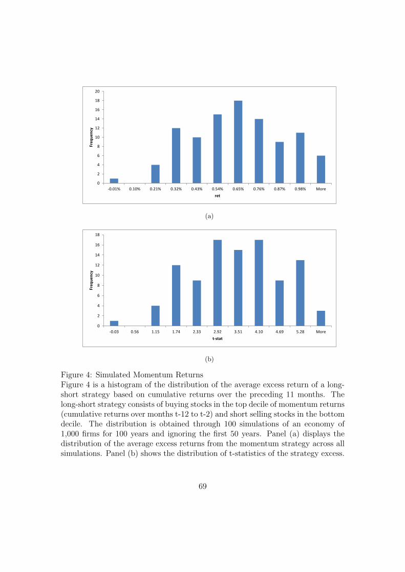
0

2

4

6

8

10

12

14

16

18

20

-0.01% 0.10% 0.21% 0.32% 0.43% 0.54% 0.65% 0.76% 0.87% 0.98% More

Frequency

ret

(a)

0

2

4

6

8

10

12

14

16

18

-0.03 0.56 1.15 1.74 2.33 2.92 3.51 4.10 4.69 5.28 More

Frequency

t-stat

(b)

Figure 4: Simulated Momentum ReturnsFigure 4 is a histogram of the distribution of the average excess return of a long-short strategy based on cumulative returns over the preceding 11 months. Thelong-short strategy consists of buying stocks in the top decile of momentum returns(cumulative returns over months t-12 to t-2) and short selling stocks in the bottomdecile. The distribution is obtained through 100 simulations of an economy of1,000 firms for 100 years and ignoring the first 50 years. Panel (a) displays thedistribution of the average excess returns from the momentum strategy across allsimulations. Panel (b) shows the distribution of t-statistics of the strategy excess.

69

0

5

10

15

20

25

-0.11% 0.01% 0.14% 0.27% 0.39% 0.52% 0.65% 0.77% 0.90% 1.03% More

Frequency

ret

(a)

0

5

10

15

20

25

-0.62 0.04 0.71 1.38 2.04 2.71 3.38 4.04 4.71 5.38 More

Frequency

t-stat

(b)

Figure 5: Simulated Profitability ReturnsFigure 5 is a histogram of the distribution of the average excess return of a long-short strategy based on firm profitability in the prior year. The long-short strategyconsists of buying stocks in the top decile of profitability (cumulative profits overthe period t-18 to t-12) and short selling stocks in the bottom decile. The distri-bution is obtained through 100 simulations of an economy of 1,000 firms for 100years and ignoring the first 50 years. Panel (a) displays the distribution of theaverage excess returns from the profitability strategy across all simulations. Panel(b) shows the distribution of t-statistics of the strategy excess return.

70