Tree growth inference and prediction from diameter censuses and ring widths

Ecological Applications, 17(7), 2007, pp. 1942–1953� 2007 by the Ecological Society of America

TREE GROWTH INFERENCE AND PREDICTION FROM DIAMETERCENSUSES AND RING WIDTHS

JAMES S. CLARK,1,2,3,4,6 MICHAEL WOLOSIN,2,3 MICHAEL DIETZE,2,3 INES IBANEZ,2,3 SHANNON LADEAU,2,3,7

MIRANDA WELSH,1 AND BRIAN KLOEPPEL5

1Nicholas School of the Environment, Duke University, Durham, North Carolina 27708 USA2Department of Biology, Duke University, Durham, North Carolina 27708 USA

3University Program in Ecology, Duke University, Durham, North Carolina 27708 USA4Institute of Statistics and Decision Sciences, Duke University, Durham, North Carolina 27708 USA

5Coweeta Hydrologic Laboratory, Otto, North Carolina 28763 USA

Abstract. Estimation of tree growth is based on sparse observations of tree diameter, ringwidths, or increments read from a dendrometer. From annual measurements on a few trees(e.g., increment cores) or sporadic measurements from many trees (e.g., diameter censuses onmapped plots), relationships with resources, tree size, and climate are extrapolated to wholestands. There has been no way to formally integrate different types of data and problems ofestimation that result from (1) multiple sources of observation error, which frequently result inimpossible estimates of negative growth, (2) the fact that data are typically sparse (a few treesor a few years), whereas inference is needed broadly (many trees over many years), (3) the factthat some unknown fraction of the variance is shared across the population, and (4) the factthat growth rates of trees within competing stands are not independent. We develop ahierarchical Bayes state space model for tree growth that addresses all of these challenges,allowing for formal inference that is consistent with the available data and the assumption thatgrowth is nonnegative. Prediction follows directly, incorporating the full uncertainty frominference with scenarios for ‘‘filling the gaps’’ for past growth rates and for future conditionsaffecting growth. An example involving multiple species and multiple stands with tree-ringdata and up to 14 years of tree census data illustrates how different levels of information at thetree and stand level contribute to inference and prediction.

Key words: Bayesian state space model; data assimilation; forest growth; hierarchical models;observation error; tree rings.

INTRODUCTION

Knowledge of tree growth is needed to understand

population dynamics (Condit et al. 1993, Fastie 1995,

Frelich and Reich 1995, Clark and Clark 1999, Wyckoff

and Clark 2002, 2005, Webster and Lorimer 2005),

species interactions (Swetnam and Lynch 1993), carbon

sequestration (DeLucia et al. 1999, Casperson et al.

2000), forest response to climate change (Cook 1987,

Graumlich et al. 1989), and restoration (Pearson and

Vitousek 2001). Despite its importance, diameter growth

estimates are limited due to the effort required for data

collection and problems associated with inference.

Estimates derive from any of three methods, diameter

measurements, tree rings, and dendrometer bands, each

with substantial uncertainty. The most common method

involves measuring tree diameters repeatedly and

calculating diameter change by subtraction. This ap-

proach has the advantages that diameters can be

measured rapidly, and it can be used in environments

where trees do not produce identifiable annual rings.

There are several disadvantages to diameter measure-

ments. Although measurement is fast, nothing is learned

until sufficient time has elapsed between observations to

allow for a confident estimate of the increment. If

interest focuses on individuals with particular growth

characteristics, those individuals may not even be

identifiable as such until years have passed. Because

intervals between measurements can be long, annual

growth rates are unknown. Instead, there is an

interpolated average growth rate for the full interval

(Biondi 1999). Long intervals may be needed, because

diameter measurements have substantial error (Biging

and Wensel 1988, Gregoire et al. 1990, Biondi 1999),

enough that diameters are frequently observed to

decrease (e.g., Clark and Clark 1999). Of course, growth

occurs each year (even ‘‘missing rings’’ may not occur

over the full circumference), so the apparent decline in

diameter results from errors in the measurements

themselves (the tape or caliper is not located at precisely

the same height and orientation on the tree), from shrink

and swell with changing bole moisture storage, or from

changes in bark thickness that are unrelated to growth

(common in pines and other thick-barked species).

Manuscript received 20 June 2006; revised 26 February 2007;accepted 22 March 2007. Corresponding Editor: Y. Luo.

6 E-mail: [email protected] Present address: Smithsonian Environmental Research

Center, P.O. Box 28, 647 Contees Wharf Road, Edgewater,Maryland 21037 USA.

1942

Various ad hoc remedies (discarding intervals of

negative growth, adding to each observation a constant

increment to insure that all increments come out

positive) introduce bias, even if one simply repeats

measurements only on the trees observed to have

negative increments (e.g., Clark and Clark 1999). In

short, diameter must have increased over the interval,

but any estimate of the increment would depend on

whatever ad hoc is used to make negative increments

come out positive.

Two alternatives to periodic tape measurements are

increment cores and dendrometer bands. They share the

advantages that annual (or sub-annual) growth can be

obtained. For increment cores, this growth rate applies to

one radius of the tree, so several increment cores may be

taken for each tree and averaged. The true area increment,

i.e., integrated over the tree circumference, is not known.

Further complications include the fact that trees may not

have identifiable growth rings, that cores are time-

consuming to obtain and analyze, and that takingmultiple

cores simultaneously or over time may affect tree health.

In temperate environments, growth rings range from

being readily identifiable (e.g., many conifers and ring-

porous hardwoods) to those having rings that are often

missed (e.g., many diffuse porous hardwoods). Like

diameter measurements, dendrometer bands provide no

information until an increment has accumulated, and the

measurements depend on timing of observations, due to

shrink and swell of the bole. The effort involved means

that increment cores and dendrometer bands are usually

obtained for sample individuals, not entire stands.

However, without full information on all trees that reside

within a known area, calculations of stand biomass

increment rely on extrapolation.

As with many ecological analyses, this one involves

several types of information (increment cores and

diameter measurements). In most cases, there is different

information available for each individual, depending on

when it was measured, if there is an increment core, and

when the increment core was taken. In the data set we

describe, some of the increment cores were obtained in

1998, others in 2005 or 2006. Diameter measurements

were obtained at irregular intervals. Stands were sampled

in different years. Some trees have more than one

increment core. If there is no increment core, how do we

exploit information that might come from the full sample

to make some probability statement about growth for a

tree having only a few diameter measurements? If there is

an increment core, how do we combine it with diameter

measurements, both of which have error?

The uncertainty associated with data suggests need for

inference, i.e., estimates of diameter and growth with

confidence envelopes. Available methods do not apply

to this problem. For diameter measurements, we can

expect to have no observations for most individuals and

years, and errors are unknown. For increment measure-

ments, a fraction of trees and years may be represented.

Growth rates vary among individuals, and this variation

can be important (Lieberman and Lieberman 1985,

Clark et al. 2003b). Sparse observations means that we

would like to borrow information across all or part of

the population as basis for ‘‘filling’’ the gaps. This need

to share information is evident in regressions used for

approximating a mean growth rate schedule for a

population (Condit et al. 1993, Terborgh et al. 1997,

Baker 2003). Regression methods that have been applied

to this problem do not exploit the full data set (by fitting

separate models for different classes of individuals) and

they do not accommodate variability contributed by

population heterogeneity (by not estimating tree-to-tree

differences). Moreover, previous regression approaches

ignore the nonindependence of observations and the

time series character of data (where multiple observa-

tions accumulate for the same individuals over time), of

the process (diameter-age estimation based on static

assumptions concerning canopy position), or of both.

The challenges of inference carry through to prediction,

which requires estimates of uncertainty in both diameter

and growth rate. Due to the errors summarized above, the

estimated confidence envelope for diameter in year t

would overlap with that for year t þ 1. A naıve Monte

Carlo simulation of tree growth based on such estimates

(drawing at random from diameter sequences) would

predict negative growth in many years. The need to avoid

this unrealistic outcome has spawned various ad hoc

methods (e.g., Lieberman and Lieberman 1985) that

involve resampling data with constraints that do not yield

a predictive interval, because they are not based on a

consistent probability model for the process and data.

In summary, methods are needed for combining

information in a way that is consistent with knowledge

that (1) growth is not negative, (2) some variation in

growth is shared among years and across individuals,

and (3) there are different types of observation errors

associated with each data type. Moreover, given

estimates of past growth, we need to know the

uncertainty associated with potential for future growth.

Often, the principle objective of growth estimation is the

perspective it can provide on how stands may develop in

the future. In light of the information available, to what

extent can we predict growth trends?

In this paper, we describe a general method for

estimating tree growth where multiple, but incomplete,

sources of information are available and for projecting

that growth forward. We develop a Bayesian state space

model of growth (Carlin et al. 1992, Calder et al. 2003,

Clark and Bjørnstad 2004), conditioned on the fact that

actual (and unknown) growth is nonnegative, that the

rate of growth is potentially informed by observations of

increment width and diameter measurements, and that

observations will be sparse, both within individual

sequences and across the stand. The Bayesian frame-

work allows exploitation of prior information on

measurement errors and ‘‘borrowing strength’’ across

the full data set(s), while responding to the amount,

type, and observation errors associated with them. We

October 2007 1943DATA ASSIMILATION FOR TREE GROWTH

simultaneously provide estimates for every individual

every year in the stand together with the stand, on

average.

DATA SETS

Growth data come from nine mapped stands in the

southern Appalachians and Piedmont of North Carolina

(Table 1), established since 1991 for purposes of

monitoring and experimental analysis of forest dynamics

(Clark et al. 1998, Beckage et al. 2000, Hille Ris Lambers

et al. 2005, Ibanez et al. 2007). Multiple diameter

measurements are available for all trees, obtained at

intervals of one to four years. The measurements are

made at breast height marked by a nail that holds a tag

indicating the identifying tree number. Increment cores

were obtained on a subset of trees in 1998 (Wyckoff and

Clark 2002) and in 2005 (M. Wolosin, J. S. Clark, and

M. Dietze, unpublished manuscript). The increment cores

were oriented with a compass, and several cores were

taken from some trees. Orientation of cores was done

only for future reference in the event that a core is taken

again from the same tree. Cores were mounted on a solid

frame, finely sanded, and measured with a sliding stage

micrometer. For purposes of demonstration we use data

on six species of Quercus (Table 1). A full analysis of all

species is reported separately (M. Wolosin, J. S. Clark,

and M. Dietze, unpublished manuscript).

DATA MODELING

Model fitting

Due to the fact that data will typically be sparse, the

model is developed to maximize the support that can be

drawn across the full data set(s), while emphasizing the

information for specific trees and years, when available.

The level of uncertainty, as represented by a confidence

envelope, reflects the combined information available

for all individuals and years. Information from the full

set of trees and years enters through the log mean

growth rate b0. Each individual is unique, with

individual differences supported by a term for random

individual effects bij, which draw on the fact that there

can be multiple diameter and growth observations for

specific individuals. There can be shared year-to-year

variation due to climate, for example, which supports an

estimate of fixed year effects bt. By modeling each of

these effects, we strike a balance between the data that

can enter in one or more ways for each tree-year and the

support that comes from the fact that some of the

variation may be shared across the population and over

time. Variation is not smoothed away: the degree of

smoothing depends on the extent to which variation is

shared across the data set, the size of the data set(s), and

the weighting of data sets. We discuss weighting after

introducing the model.

Let Dij,t be the diameter in centimeters of tree i in

stand j in year t, and Xij,t be the diameter increment

added between year t and tþ 1. We develop a model of

growth (Fig. 1) that exploits the information on overall

tree growth, with log mean for the full population b0,random individual effects bij (how tree ij differs from the

rest of the population), and fixed year effects bt (therecan be shared year-to-year variation due to, say,

climate). Because growth must be positive, we model

log increments,

lnðXij;tÞ[ lnðDij;tþ1 � Dij;tÞ ¼ lij;t þ eij;t ð1Þ

as a linear equation with population log mean growth

rate b0, random individual effect bij, year effect bt, and

TABLE 1. Number of Quercus trees and sample sizes for each of the stands included in this analysis.

Stand C1 C2 C3 C4 C5 CL CU D1 D2 Total

Beginning year 1992 1992 1992 1992 1992 2000 2000 2000 1999Increment observed 379 282 294 346 80 300 255 938 0 2874�Diameter observed 874 204 571 789 112 1219 1081 1267 460 6577�Tree-years 3472 800 2016 2784 384 2992 2392 3344 1656 19 840§Q. alba 12 0 0 0 1 0 0 229 65 307Q. coccinea 25 7 1 14 0 41 44 0 0 132Q. falcata 0 0 0 0 0 0 0 19 7 26Q. marilandica 10 0 0 0 0 0 0 20 0 30Q. phellos 0 0 0 0 0 0 1 18 71 90Q. montana 88 32 99 101 0 176 173 0 0 669Q. rubra 38 5 19 56 23 132 49 60 2 384Q. stellata 0 0 0 0 0 0 0 41 39 80Q. velutina 44 6 7 3 0 8 14 29 0 111Species uncertain 0 0 0 0 0 17 18 2 0 37Total trees 217 50 126 174 24 374 299 418 184 1866}

Notes: Sample sizes are for each of nine stands included in this analysis of Quercus. Stands are located at the CoweetaHydrologic Lab (C in stand name) or the Duke Forest (D in stand name). Beginning year is the year in which diametermeasurements began; increment observed is the number of growth increments measured from increment cores; diameter observed isthe number of diameters measured using a tape; tree-years is the total number of diameter estimates; and total trees is the totalnumber of trees, not tree years.

� Total ¼ nI.� Total ¼ nD.§ Total¼ n.} Total ¼ nT.

JAMES S. CLARK ET AL.1944 Ecological ApplicationsVol. 17, No. 7

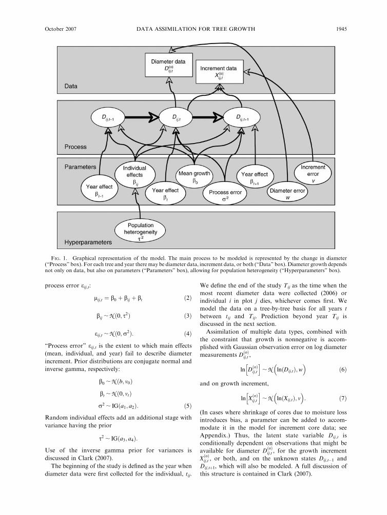
process error eij,t:

lij;t ¼ b0 þ bij þ bt ð2Þ

bij ; N ð0; s2Þ ð3Þ

eij;t ; N ð0;r2Þ: ð4Þ

‘‘Process error’’ eij,t is the extent to which main effects

(mean, individual, and year) fail to describe diameter

increment. Prior distributions are conjugate normal and

inverse gamma, respectively:

b0 ; N ðb; v0Þ

bt ; N ð0; vtÞ

r2 ; IGða1; a2Þ: ð5Þ

Random individual effects add an additional stage with

variance having the prior

s2 ; IGða3; a4Þ:

Use of the inverse gamma prior for variances is

discussed in Clark (2007).

The beginning of the study is defined as the year when

diameter data were first collected for the individual, tij.

We define the end of the study Tij as the time when the

most recent diameter data were collected (2006) or

individual i in plot j dies, whichever comes first. We

model the data on a tree-by-tree basis for all years t

between tij and Tij. Prediction beyond year Tij is

discussed in the next section.

Assimilation of multiple data types, combined with

the constraint that growth is nonnegative is accom-

plished with Gaussian observation error on log diameter

measurements DðoÞij;t ,

ln DðoÞij;t

h i; N

�lnðDij;tÞ;w

�ð6Þ

and on growth increment,

ln XðoÞij;t

h i; N

�lnðXij;tÞ; v

�: ð7Þ

(In cases where shrinkage of cores due to moisture loss

introduces bias, a parameter can be added to accom-

modate it in the model for increment core data; see

Appendix.) Thus, the latent state variable Dij,t is

conditionally dependent on observations that might be

available for diameter DðoÞij;t , for the growth increment

XðoÞij;t , or both, and on the unknown states Dij,t�1 and

Dij,tþ1, which will also be modeled. A full discussion of

this structure is contained in Clark (2007).

FIG. 1. Graphical representation of the model. The main process to be modeled is represented by the change in diameter(‘‘Process’’ box). For each tree and year there may be diameter data, increment data, or both (‘‘Data’’ box). Diameter growth dependsnot only on data, but also on parameters (‘‘Parameters’’ box), allowing for population heterogeneity (‘‘Hyperparameters’’ box).


Nonindependence of data is accommodated by the

stochastic treatment of the underlying process. We are

jointly modeling growth of interacting plants. It has long

been known that growth rates of competing plants

cannot be treated as independent observations (e.g.,

Mitchell-Olds 1987). A simple analysis of multiple

interacting trees would violate this most fundamental

assumption about the distribution of data. Our hierar-

chical approach accommodates correlations among

observations (both within and among trees), because

those relationships are taken up at the process stage.

Consider a single tree-year for which there are both

increment and diameter data. Here is their joint

probability (conditioned on the rest of the model):

p½DðoÞij;t ;XðoÞij;t ;Dij;t� ¼ p½DðoÞij;t ;X

ðoÞij;t jDij;t�pðDij;tÞ

¼ p½DðoÞij;t jDij;t�p½XðoÞij;t jDij;t�pðDij;tÞ

¼ N�

ln½DðoÞij;t �jlnðDij;tÞ;w�

3 N�

ln½XðoÞij;t �jlnðDij;tþ1 � Dij;tÞ; v�

3 N�

lnðDij;tþ1 � Dij;tÞjlij;t;r2�:

The densities in the last line are, respectively, diameter

data model, increment data model, and process model.

The two data models are connected by way of their

relationship to the process model. If Dij,t is not

stochastic, we cannot claim that the two data types

bring new information. Each is just a deterministic

transform of the other. Placing independent data models

on each would be inconsistent. This incorrect assump-

tion is implicit if we replace the third factor (a density)

with a constant value. Once we admit uncertainty in Dij,t

we allow for the possibility of conditional independence

between data types: both data types might have errors

that are independent (conditional on Dij,t), because

errors in measuring tree rings are unrelated to errors in

measurements of tree diameter.

Stochasticity in our process model includes process

error and random effects (Eqs. 1–4). The random effects

could be spatial, involving inter-tree distances. If such an

effect were evident, we could have included part of this

interdependence as a fixed effect, using a competitive

index involving size and distance. Had we included such

a fixed effect, we would still want to explore additional

random effects that are not accommodated by such

indices. We did not include such effects in this model,

because there are no trends in diameter increments in

our data that are correlated with distances among trees

or locations within stands. Clark (2007) provides an

example showing how the spatial random effect can be

modeled with Bayesian kriging. Although there is no

spatial pattern in random effects for these data,

variation among individuals cannot be ignored. Here,

the variation is large, albeit not well described by simple

spatial relationships. The fact that random effects are

nonspatial (no evidence of a crowding effect on growth)

is not surprising. With few exceptions, all trees in this

analysis are crowded. Had we analyzed a data set with a

range of crowing levels we would expect to see a spatial

trend in random effects.

Prior parameter values allow for a weighting of the

multiple data types, and they admit knowledge of the

approximate ranges of variability in measurements to be

expected. Priors for observation errors are conjugate

inverse gamma:

v ; IGða5; a6Þ ð8aÞ

w ; IGða7; a8Þ: ð8bÞ

There is a natural weighting that comes from measure-

ment errors. To see this, consider the conditional

posterior for a growth increment Xij,t ¼ Dij,tþ1 � Dij,t,

for which there exist an increment measurement and

diameter measurements for year t and tþ 1:

pðXij;t � � �Þ } N�

lnðXij;tÞjlij;t;r2�

N�

ln½XðoÞij;t �jlnðXij;tÞ; v�

3 N�

DðoÞij;t jDij;t;w

�N�

DðoÞij;tþ1jDij;tþ1;w

�:

ð9aÞ

By contrast, the conditional posterior for a growth year

with no observations is

pðXij;t � � �Þ ¼ N�

lnðXij;tÞjlij;t;r2�: ð9bÞ

For a tree increment with both types of observations

(Eq. 9a), (1) diameter measurements DðoÞij;t will have large

impact if their variance w is small (Eq. 6), (2) increment

measurements XðoÞij;t will have large impact if their

variance v is small (Eq. 7), and (3) the degree to which

the estimate will be influenced by the full data set will

increase with decreasing variance r2 (Eqs. 1 and 2).

Prior information not only informs these estimates, but

it also weights their contributions. We select priors that

bring in what is known about the measurement errors w

and v, but weight both to insure that measurements

dominate over the population model (Eqs. 1 and 2). In

other words, we want the relationship between w and v

to reflect what is known about errors in both

observations, while insuring that both carry much more

weight than r2. This is a subjective decision to

emphasize blending of data, rather than smoothing

over variability. With this approach the process model

has most impact for tree years having no data. From

multiple measurements of trees and increment cores

(e.g., Wyckoff and Clark 2005; M. Wolosin, J. S. Clark,

and M. Dietze, unpublished manuscript) we know

standard deviations are approximately 1 cm and 0.01

cm, respectively. Variances are on a log scale in the

model, reflecting the fact that errors proportionately

increase with tree diameter and decrease with increment


width (values � 1). Diameter measurements with an

error variance of 1 cm have a variance on log error from

0.0004 (50 cm diameter trees) to 0.01 (10 cm diameter

trees). Increment measurements with an error variance

of 0.0001 (standard deviation of 0.01 cm) have a

variance on log increment from 0.001 (0.3 cm incre-

ment) to 0.01 (0.1 cm increment). Thus, informative

priors can be centered on 0.001 to 0.01 for both types of

data. We used priors for these variances with mean

values of 0.01 (v) and 0.001 (w). Posteriors are

insensitive to the precise values of these priors. We then

weight these variances such that each is 10 times the

number of observations:

a5 ¼ 10nI

a6 ¼ 0:01ða5 � 1Þ

a7 ¼ 10nD

a8 ¼ 0:001ða7 � 1Þ

where nI and nD are the number of increment and

diameter observations, respectively (Table 1). This

weighting is based on moment matching (Clark 2007).

By contrast, we use a large prior mean on r2 of 1, and

weight it to be 100 times less than the number of tree

years:

n ¼X

ij

ðTij � tijÞ ¼ 19 840

a1 ¼ n=100

a2 ¼ a1 � 1:

Because n is large, we effectively downweight the

population model (Eqs. 1 and 2) to insure minimal

smoothing. This will dominant for tree years for which

there are no observations (Eq. 9b).

Other priors are proper, but noninformative. The

prior on log mean growth rate has mean and variance b

¼�2 (i.e., a prior mean growth rate of e�2¼ 0.13 cm/yr)

and v0 ¼ 1 3 107/n. This prior is 1 3 107 times weaker

than the sample size (total number of tree years). The

prior mean for the variance of random effects s2 was setto an arbitrary value of 1, and weighted roughly 0.01 of

the data. This is accomplished with a3 ¼ nT/100, where

nT is the number of trees (Table 1). Year effects bt haveprior mean zero and vt¼ 1. Posterior distributions were

not influenced by the mean values selected for b0, s2, and

bt, because priors were weak.

Analysis of the model is accomplished by Gibbs

sampling (Gelfand and Smith 1990), implementation of

which is discussed in the Appendix.

Prediction

We use a Bayesian prediction framework to forecast

growth several years ahead. The predictive density for

diameter one year ahead is represented by the integral

p�

Dij;Tijþ1j DðoÞij;t

n o; X

ðoÞij;t

n o; b��

¼ZZ

p�

Dij;Tijþ1j DðoÞij;t

n o; X

ðoÞij;t

n o; b�Tijþ1; h

�

3 p�hj D

ðoÞij;t

n o; X

ðoÞij;t

n o�pðb�Tijþ1jb

�Þdhdb�Tijþ1

ð10Þ

where

h [½ Dij;t

� �; lij;t

� �; b0; bij

� �; btf g;r2; s2;w; v�

is the set of parameters and latent variables estimated

from the model, and p(h j fDðoÞij;t g, fXðoÞij;t g) is the joint

posterior, conditioned on all diameter and increment data.

To simplify notation, we have omitted the prior parameter

values from the left hand side of Eq. 10. This predictive

distribution mixes over the uncertainty in parameter

estimates (the inner integral is taken over the posterior),

and over the uncertainty in the scenario for the year Tijþ1. The scenario is expressed in terms of the effect for the

upcoming year, b�ij;Tijþ1, the uncertainty of which is

described by density p(b�ij;Tijþ1 j b�) and written condition-

ally to remind us that the prediction will depend on

whatever assumptions b� went into the construction of

this scenario. The outer integral incorporates this scenario

uncertainty (Draper et al. 1999, Clark 2007). The scenario

could involve assumptions about growth conditions in

future years, expressed in terms of the density

p(b�ij;Tijþ1 j b�). In fact, we do not actually solve this

integral, but rather useMonte Carlo simulation. Using the

same approach, we can predict further ahead, expecting

the uncertainty to increase as we consider years further

into the future. This uncertainty magnifies if we allow that

the uncertainty in growing conditions (the scenario

b�ij;Tijþk, where k is taken in years) might likewise increase.

Because we expect predictive capacity to decline, we limit

predictions to a lead time of k¼ 10 yr.

RESULTS

Several parameters describe a population-wide pat-

tern in the data. In this analysis of 10 Quercus species

(Table 1), all parameters are well identified, as indicated

by narrow credible intervals (Table 2). Error parameter

estimates reflect priors. The informative prior insures

that the posterior estimate of r2 is centered at the large

value of 1. Large weights on w and v insure that they

dominate for individuals and years with observations.

The standard deviation for random individual effects shad a posterior mean of 0.536, substantially lower than

the prior mean value, and selected to be non-informa-

tive.

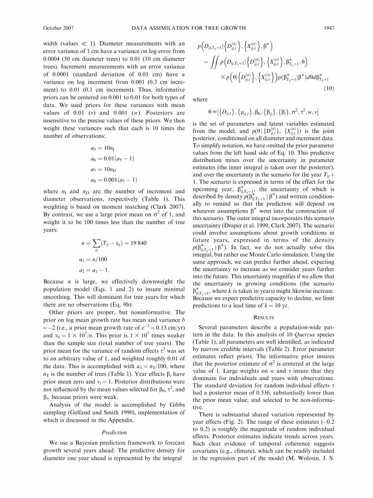
There is substantial shared variation represented by

year effects (Fig. 2). The range of these estimates (�0.2to 0.2) is roughly the magnitude of random individual

effects. Posterior estimates indicate trends across years.

Such clear evidence of temporal coherence suggests

covariates (e.g., climate), which can be readily included

in the regression part of the model (M. Wolosin, J. S.


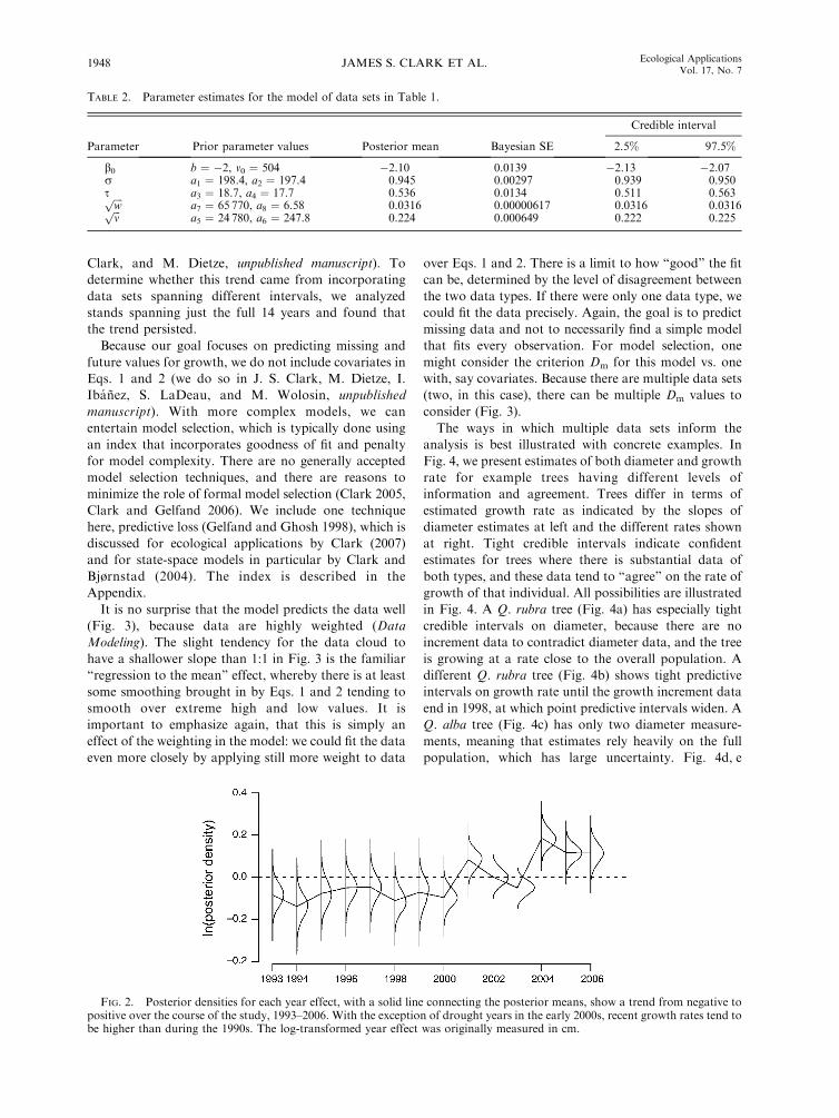
Clark, and M. Dietze, unpublished manuscript). To

determine whether this trend came from incorporating

data sets spanning different intervals, we analyzed

stands spanning just the full 14 years and found that

the trend persisted.

Because our goal focuses on predicting missing and

future values for growth, we do not include covariates in

Eqs. 1 and 2 (we do so in J. S. Clark, M. Dietze, I.

Ibanez, S. LaDeau, and M. Wolosin, unpublished

manuscript). With more complex models, we can

entertain model selection, which is typically done using

an index that incorporates goodness of fit and penalty

for model complexity. There are no generally accepted

model selection techniques, and there are reasons to

minimize the role of formal model selection (Clark 2005,

Clark and Gelfand 2006). We include one technique

here, predictive loss (Gelfand and Ghosh 1998), which is

discussed for ecological applications by Clark (2007)

and for state-space models in particular by Clark and

Bjørnstad (2004). The index is described in the

Appendix.

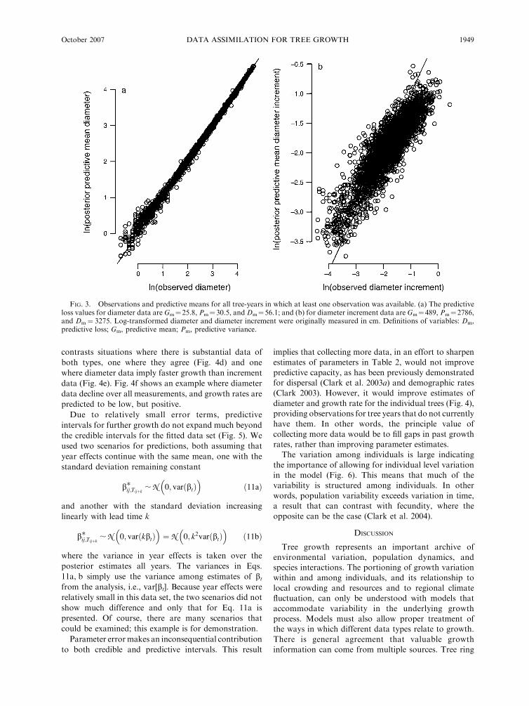
It is no surprise that the model predicts the data well

(Fig. 3), because data are highly weighted (Data

Modeling). The slight tendency for the data cloud to

have a shallower slope than 1:1 in Fig. 3 is the familiar

‘‘regression to the mean’’ effect, whereby there is at least

some smoothing brought in by Eqs. 1 and 2 tending to

smooth over extreme high and low values. It is

important to emphasize again, that this is simply an

effect of the weighting in the model: we could fit the data

even more closely by applying still more weight to data

over Eqs. 1 and 2. There is a limit to how ‘‘good’’ the fit

can be, determined by the level of disagreement between

the two data types. If there were only one data type, we

could fit the data precisely. Again, the goal is to predict

missing data and not to necessarily find a simple model

that fits every observation. For model selection, one

might consider the criterion Dm for this model vs. one

with, say covariates. Because there are multiple data sets

(two, in this case), there can be multiple Dm values to

consider (Fig. 3).

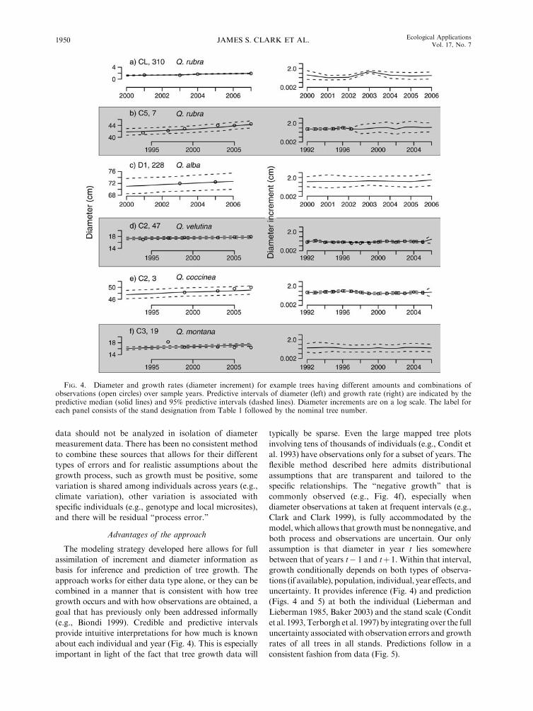
The ways in which multiple data sets inform the

analysis is best illustrated with concrete examples. In

Fig. 4, we present estimates of both diameter and growth

rate for example trees having different levels of

information and agreement. Trees differ in terms of

estimated growth rate as indicated by the slopes of

diameter estimates at left and the different rates shown

at right. Tight credible intervals indicate confident

estimates for trees where there is substantial data of

both types, and these data tend to ‘‘agree’’ on the rate of

growth of that individual. All possibilities are illustrated

in Fig. 4. A Q. rubra tree (Fig. 4a) has especially tight

credible intervals on diameter, because there are no

increment data to contradict diameter data, and the tree

is growing at a rate close to the overall population. A

different Q. rubra tree (Fig. 4b) shows tight predictive

intervals on growth rate until the growth increment data

end in 1998, at which point predictive intervals widen. A

Q. alba tree (Fig. 4c) has only two diameter measure-

ments, meaning that estimates rely heavily on the full

population, which has large uncertainty. Fig. 4d, e

FIG. 2. Posterior densities for each year effect, with a solid line connecting the posterior means, show a trend from negative topositive over the course of the study, 1993–2006. With the exception of drought years in the early 2000s, recent growth rates tend tobe higher than during the 1990s. The log-transformed year effect was originally measured in cm.

TABLE 2. Parameter estimates for the model of data sets in Table 1.

Parameter Prior parameter values Posterior mean Bayesian SE

Credible interval

2.5% 97.5%

b0 b ¼ �2, v0 ¼ 504 �2.10 0.0139 �2.13 �2.07r a1 ¼ 198.4, a2 ¼ 197.4 0.945 0.00297 0.939 0.950s a3 ¼ 18.7, a4 ¼ 17.7 0.536 0.0134 0.511 0.563ffiffiffiffi

wp

a7 ¼ 65 770, a8 ¼ 6.58 0.0316 0.00000617 0.0316 0.0316ffiffiffivp

a5 ¼ 24 780, a6 ¼ 247.8 0.224 0.000649 0.222 0.225


contrasts situations where there is substantial data of

both types, one where they agree (Fig. 4d) and one

where diameter data imply faster growth than increment

data (Fig. 4e). Fig. 4f shows an example where diameter

data decline over all measurements, and growth rates are

predicted to be low, but positive.

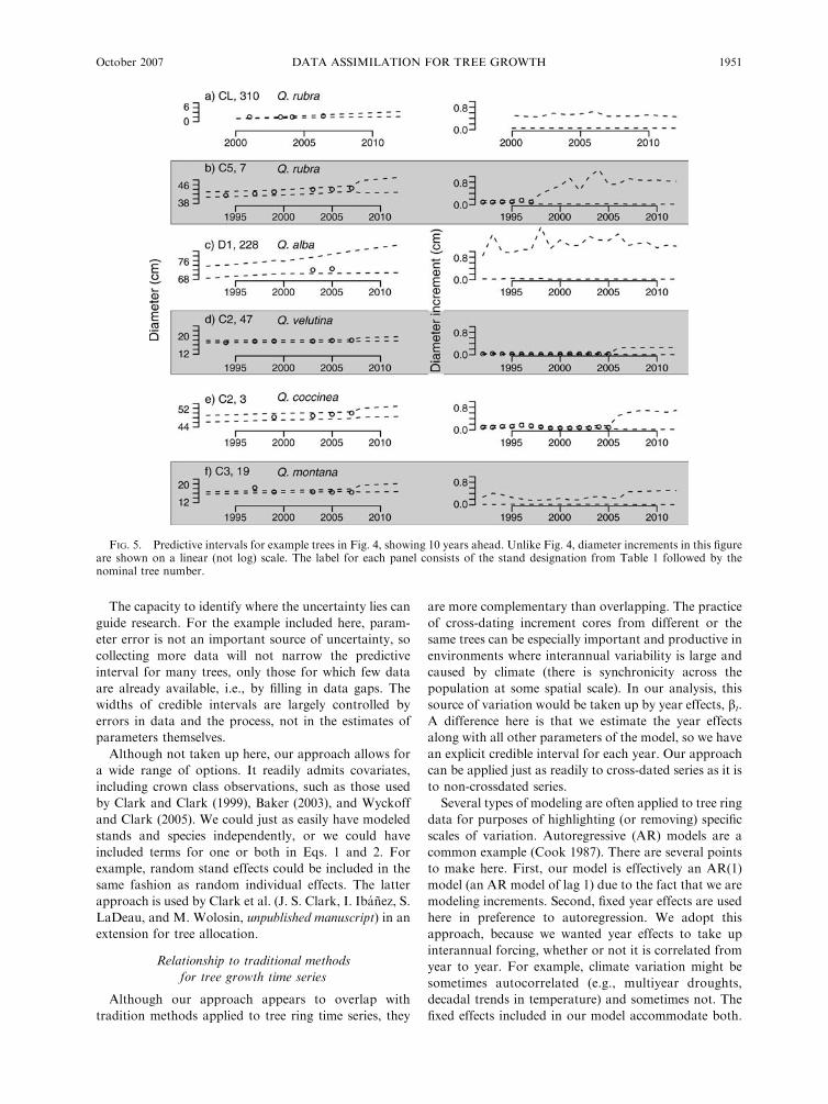
Due to relatively small error terms, predictive

intervals for further growth do not expand much beyond

the credible intervals for the fitted data set (Fig. 5). We

used two scenarios for predictions, both assuming that

year effects continue with the same mean, one with the

standard deviation remaining constant

b�ij;Tijþk; N

�0; varðbtÞ

�ð11aÞ

and another with the standard deviation increasing

linearly with lead time k

b�ij;Tijþk; N

�0; varðkbtÞ

�¼ N

�0; k2varðbtÞ

�ð11bÞ

where the variance in year effects is taken over the

posterior estimates all years. The variances in Eqs.

11a, b simply use the variance among estimates of btfrom the analysis, i.e., var[bt]. Because year effects were

relatively small in this data set, the two scenarios did not

show much difference and only that for Eq. 11a is

presented. Of course, there are many scenarios that

could be examined; this example is for demonstration.

Parameter errormakes an inconsequential contribution

to both credible and predictive intervals. This result

implies that collecting more data, in an effort to sharpen

estimates of parameters in Table 2, would not improve

predictive capacity, as has been previously demonstratedfor dispersal (Clark et al. 2003a) and demographic rates

(Clark 2003). However, it would improve estimates of

diameter and growth rate for the individual trees (Fig. 4),providing observations for tree years that do not currently

have them. In other words, the principle value of

collecting more data would be to fill gaps in past growthrates, rather than improving parameter estimates.

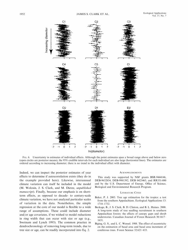
The variation among individuals is large indicating

the importance of allowing for individual level variationin the model (Fig. 6). This means that much of the

variability is structured among individuals. In other

words, population variability exceeds variation in time,a result that can contrast with fecundity, where the

opposite can be the case (Clark et al. 2004).

DISCUSSION

Tree growth represents an important archive of

environmental variation, population dynamics, andspecies interactions. The portioning of growth variation

within and among individuals, and its relationship to

local crowding and resources and to regional climatefluctuation, can only be understood with models that

accommodate variability in the underlying growth

process. Models must also allow proper treatment ofthe ways in which different data types relate to growth.

There is general agreement that valuable growth

information can come from multiple sources. Tree ring

FIG. 3. Observations and predictive means for all tree-years in which at least one observation was available. (a) The predictiveloss values for diameter data are Gm¼25.8, Pm¼30.5, and Dm¼56.1; and (b) for diameter increment data are Gm¼489, Pm¼2786,and Dm¼ 3275. Log-transformed diameter and diameter increment were originally measured in cm. Definitions of variables: Dm,predictive loss; Gm, predictive mean; Pm, predictive variance.


data should not be analyzed in isolation of diameter

measurement data. There has been no consistent method

to combine these sources that allows for their different

types of errors and for realistic assumptions about the

growth process, such as growth must be positive, some

variation is shared among individuals across years (e.g.,

climate variation), other variation is associated with

specific individuals (e.g., genotype and local microsites),

and there will be residual ‘‘process error.’’

Advantages of the approach

The modeling strategy developed here allows for full

assimilation of increment and diameter information as

basis for inference and prediction of tree growth. The

approach works for either data type alone, or they can be

combined in a manner that is consistent with how tree

growth occurs and with how observations are obtained, a

goal that has previously only been addressed informally

(e.g., Biondi 1999). Credible and predictive intervals

provide intuitive interpretations for how much is known

about each individual and year (Fig. 4). This is especially

important in light of the fact that tree growth data will

typically be sparse. Even the large mapped tree plots

involving tens of thousands of individuals (e.g., Condit et

al. 1993) have observations only for a subset of years. The

flexible method described here admits distributional

assumptions that are transparent and tailored to the

specific relationships. The ‘‘negative growth’’ that is

commonly observed (e.g., Fig. 4f), especially when

diameter observations at taken at frequent intervals (e.g.,

Clark and Clark 1999), is fully accommodated by the

model, which allows that growthmust be nonnegative, and

both process and observations are uncertain. Our only

assumption is that diameter in year t lies somewhere

between that of years t� 1 and tþ1. Within that interval,

growth conditionally depends on both types of observa-

tions (if available), population, individual, year effects, and

uncertainty. It provides inference (Fig. 4) and prediction

(Figs. 4 and 5) at both the individual (Lieberman and

Lieberman 1985, Baker 2003) and the stand scale (Condit

et al. 1993, Terborgh et al. 1997) by integrating over the full

uncertainty associated with observation errors and growth

rates of all trees in all stands. Predictions follow in a

consistent fashion from data (Fig. 5).

FIG. 4. Diameter and growth rates (diameter increment) for example trees having different amounts and combinations ofobservations (open circles) over sample years. Predictive intervals of diameter (left) and growth rate (right) are indicated by thepredictive median (solid lines) and 95% predictive intervals (dashed lines). Diameter increments are on a log scale. The label foreach panel consists of the stand designation from Table 1 followed by the nominal tree number.


The capacity to identify where the uncertainty lies can

guide research. For the example included here, param-

eter error is not an important source of uncertainty, so

collecting more data will not narrow the predictive

interval for many trees, only those for which few data

are already available, i.e., by filling in data gaps. The

widths of credible intervals are largely controlled by

errors in data and the process, not in the estimates of

parameters themselves.

Although not taken up here, our approach allows for

a wide range of options. It readily admits covariates,

including crown class observations, such as those used

by Clark and Clark (1999), Baker (2003), and Wyckoff

and Clark (2005). We could just as easily have modeled

stands and species independently, or we could have

included terms for one or both in Eqs. 1 and 2. For

example, random stand effects could be included in the

same fashion as random individual effects. The latter

approach is used by Clark et al. (J. S. Clark, I. Ibanez, S.

LaDeau, and M. Wolosin, unpublished manuscript) in an

extension for tree allocation.

Relationship to traditional methods

for tree growth time series

Although our approach appears to overlap with

tradition methods applied to tree ring time series, they

are more complementary than overlapping. The practice

of cross-dating increment cores from different or the

same trees can be especially important and productive in

environments where interannual variability is large and

caused by climate (there is synchronicity across the

population at some spatial scale). In our analysis, this

source of variation would be taken up by year effects, bt.

A difference here is that we estimate the year effects

along with all other parameters of the model, so we have

an explicit credible interval for each year. Our approach

can be applied just as readily to cross-dated series as it is

to non-crossdated series.

Several types of modeling are often applied to tree ring

data for purposes of highlighting (or removing) specific

scales of variation. Autoregressive (AR) models are a

common example (Cook 1987). There are several points

to make here. First, our model is effectively an AR(1)

model (an AR model of lag 1) due to the fact that we are

modeling increments. Second, fixed year effects are used

here in preference to autoregression. We adopt this

approach, because we wanted year effects to take up

interannual forcing, whether or not it is correlated from

year to year. For example, climate variation might be

sometimes autocorrelated (e.g., multiyear droughts,

decadal trends in temperature) and sometimes not. The

fixed effects included in our model accommodate both.

FIG. 5. Predictive intervals for example trees in Fig. 4, showing 10 years ahead. Unlike Fig. 4, diameter increments in this figureare shown on a linear (not log) scale. The label for each panel consists of the stand designation from Table 1 followed by thenominal tree number.


Indeed, we can inspect the posterior estimates of year

effects to determine if autocorrelation exists (they do in

the example provided here). Likewise, interannual

climate variation can itself be included in the model

(M. Wolosin, J. S. Clark, and M. Dietze, unpublished

manuscript). Finally, because our emphasis is on short-

term effects, as opposed to decade- to century-scale

climate variation, we have not analyzed particular scales

of variation in the data. Nonetheless, the simple

regression at the core of our model is flexible to a wide

range of assumptions. These could include diameter

and/or age covariates, if we wished to model reductions

in ring width that can occur with size or age (e.g.,

Swetnam and Lynch 1993). The common practice in

dendrochronology of removing long-term trends, due to

tree size or age, can be readily incorporated into Eq. 2.

ACKNOWLEDGMENTS

This study was supported by NSF grants BSR-9444146,

DEB-9632854, DEB-9981392, DEB 0425465, and RR551-080

and by the U.S. Department of Energy, Office of Science,

Biological and Environmental Research Program.

LITERATURE CITED

Baker, P. J. 2003. Tree age estimation for the tropics: a test

from the southern Appalachians. Ecological Applications 13:

1718–1732.

Beckage, B., J. S. Clark, B. D. Clinton, and B. L. Haines. 2000.

A long-term study of tree seedling recruitment in southern

Appalachian forests: the effects of canopy gaps and shrub

understories. Canadian Journal of Forest Research 30:1617–

1631.

Biging, G. S., and L. C. Wensel. 1988. The effect of eccentricity

on the estimation of basal area and basal area increment of

coniferous trees. Forest Science 32:621–633.

FIG. 6. Uncertainty in estimates of individual effects. Although the point estimates span a broad range above and below zero(open circles are posterior means), the 95% credible intervals for each individual are also large (horizontal lines). The estimates areordered according to increasing diameter; there is no trend in the individual effect with diameter.


Biondi, F. 1999. Comparing tree-ring chronologies andrepeated timber inventories as forest monitoring tools.Ecological Applications 9:216–227.

Calder, K., M. Lavine, P. Mueller, and J. S. Clark. 2003.Incorporating multiple sources of stochasticity in populationdynamic models. Ecology 84:1395–1402.

Carlin, B. P., N. G. Polson, and D. S. Stoffer. 1992. A MonteCarlo approach to nonnormal and nonlinear state-spacemodeling. Journal of the American Statistical Association 87:493–500.

Casperson, J. P., S. W. Pacala, J. C. Jenkins, G. C. Hurtt, P. R.Moorcroft, and R. A. Birdsey. 2000. Contributions of land-use history to carbon accumulation in US forests. Science290:1148–1151.

Clark, D. A., and D. B. Clark. 1999. Assessing the growth oftropical rain forest trees: issues for forest modeling andmanagement. Ecological Applications 9:981–997.

Clark, J. S. 2003. Uncertainty in population growth ratescalculated from demography: the hierarchical approach.Ecology 84:1370–1381.

Clark, J. S. 2005. Why environmental scientists are becomingBayesians. Ecology Letters 8:2–14.

Clark, J. S. 2007. Models for ecological data. PrincetonUniversity Press, Princeton, New Jersey, USA.

Clark, J. S., and O. Bjørnstad. 2004. Population time series:process variability, observation errors, missing values, lags,and hidden states. Ecology 85:3140–3150.

Clark, J. S., and A. E. Gelfand. 2006. A future for models anddata in ecology. Trends in Ecology and Evolution 21:375–380.

Clark, J. S., S. LaDeau, and I. Ibanez. 2004. Fecundity of treesand the colonization–competition hypothesis. EcologicalMonographs 74:415–442.

Clark, J. S., M. Lewis, J. S. McLachlan, and J. Hille RisLambers. 2003a. Estimating population spread: what can weforecast and how well? Ecology 84:1979–1988.

Clark, J. S., E. Macklin, and L. Wood. 1998. Stages and spatialscales of recruitment limitation in southern Appalachianforests. Ecological Monographs 68:213–235.

Clark, J. S., J. Mohan, M. Dietze, and I. Ibanez. 2003b.Coexistence: how to identify trophic trade-offs. Ecology 84:17–31.

Condit, R., S. P. Hubbell, and R. B. Foster. 1993. Identifyingfast-growing native trees from the Neotropics using datafrom a large, permanent census plot. Forest Ecology andManagement 62:123–143.

Cook, E. R. 1987. The decomposition of tree-ring series forenvironmental studies. Tree-Ring Bulletin 47:37–59.

DeLucia, E. H., J. G. Hamilton, S. L. Naidu, R. B. Thomas,J. A. Andrews, A. Finzi, M. Lavine, R. Matamala, J. E.Mohan, G. R. Hendrey, and W. H. Schlesinger. 1999. Netprimary production of a forest ecosystem with experimentalCO2 enrichment. Science 284:1177–1179.

Draper, D., A. Pereira, P. Prado, A. Saltelli, R. Cheal, S.Eguilior, B. Mendes, and S. Tarantola. 1999. Scenario and

parametric uncertainty in GESAMAC: a methodologicalstudy in nuclear waste disposal risk assessment. ComputerPhysics Communications 117:142–155.

Fastie, C. L. 1995. Causes and ecosystem consequences ofmultiple pathways of primary succession at Glacier Bay,Alaska. Ecology 76:1899–1916.

Frelich, L. E., and P. B. Reich. 1995. Spatial patterns andsuccession in a Minnesota southern-boreal forest. EcologicalMonographs 65:325–346.

Gelfand, A. E., and S. K. Ghosh. 1998. Model choice: aminimum posterior predictive loss approach. Biometrika 85:1–11.

Gelfand, A. E., and A. F. M. Smith. 1990. Sampling-basedapproaches to calculating marginal densities. Journal of theAmerican Statistical Association 85:398–409.

Graumlich, L. J., L. B. Brubaker, and C. C. Grier. 1989: Long-term trends in forest net primary productivity: CascadeMountains, Washington. Ecology 70:405–410.

Gregoire, T. G., S. M. Zedaker, and N. S. Nicholas. 1990.Modeling relative error in stem basal area estimates.Canadian Journal of Forest Research 20:496–502.

Hille Ris Lambers, J., J. S. Clark, and M. Lavine. 2005. Seedbanking in temperate forests: implications for recruitmentlimitation. Ecology 86:85–95.

Ibanez, I., J. S. Clark, S. LaDeau, and J. Hille Ris Lambers.2007. Exploiting temporal variability to understand treerecruitment response to climate change. Ecological Mono-graphs 77:163–177.

Lieberman, M., and D. Lieberman. 1985. Simulation of growthcurves from periodic increment data. Ecology 66:632–635.

Mitchell-Olds, T. 1987. Analysis of local variation in plant size.Ecology 68:82–87.

Pearson, H. L., and P. M. Vitousek. 2001. Stand dynamics,nitrogen accumulation, and symbiotic nitrogen fixation inregenerating stands of Acacia koa. Ecological Applications11:1381–1394.

Swetnam, T. W., and A. M. Lynch. 1993. Multicentury,regional-scale patterns of western spruce budworm out-breaks. Ecological Monographs 63:399–424.

Terborgh, J. C. F., P. Mueller, and L. Davenport. 1997.Estimating the ages of successional stands of tropical treesfrom growth increments. Journal of Tropical Ecology 14:833–856.

Webster, C. R., and C. G. Lorimer. 2005. Minimum openingsizes for canopy recruitment of midtolerant tree species: aretrospective approach. Ecological Applications 15:1245–1262.

Wyckoff, P. H., and J. S. Clark. 2002. Growth and mortalityfor seven co-occurring tree species in the southern Appala-chian Mountains: implications for future forest composition.Journal of Ecology 90:604–615.

Wyckoff, P., and J. S. Clark. 2005. Comparing predictors oftree growth: the case for exposed canopy area. CanadianJournal of Forest Research 35:13–20.

APPENDIX

Tree growth inference and prediction (Ecological Archives A017-077-A1).


Tree growth inference and prediction from diameter censuses and ring widths

Documents

Transcript of Tree growth inference and prediction from diameter censuses and ring widths