Citation: Ahmed Zaib, M.; Waqar, A.;

Abbas, S.; Badshah, S.; Ahmad, S.;

Amjad, M.; Rahimian Koloor, S.S.;

Eldessouki, M. Effect of Blade

Diameter on the Performance of

Horizontal-Axis Ocean Current

Turbine. Energies 2022, 15, 5323.

https://doi.org/10.3390/en15155323

Academic Editor: Francesco

Castellani

Received: 10 June 2022

Accepted: 18 July 2022

Published: 22 July 2022

Publisher’s Note: MDPI stays neutral

with regard to jurisdictional claims in

published maps and institutional affil-

iations.

Copyright: © 2022 by the authors.

Licensee MDPI, Basel, Switzerland.

This article is an open access article

distributed under the terms and

conditions of the Creative Commons

Attribution (CC BY) license (https://

creativecommons.org/licenses/by/

4.0/).

energies

Article

Effect of Blade Diameter on the Performance of Horizontal-AxisOcean Current TurbineMansoor Ahmed Zaib 1, Arbaz Waqar 1, Shoukat Abbas 1, Saeed Badshah 1 , Sajjad Ahmad 1,*,Muhammad Amjad 1 , Seyed Saeid Rahimian Koloor 2 and Mohamed Eldessouki 2,3,4,*

1 Department of Mechanical Engineering, International Islamic University, Islamabad 44000, Pakistan;mansoor.bsme713@iiu.edu.pk (M.A.Z.); arbazwaqar0@gmail.com (A.W.);shoukatabbas1997@gmail.com (S.A.); saeed.badshah@iiu.edu.pk (S.B.); m.amjad@iiu.edu.pk (M.A.)

2 Institute for Nanomaterials, Advanced Technologies and Innovation (CXI), Technical University ofLiberec (TUL), Studentska 2, 461 17 Liberec, Czech Republic; s.s.r.koloor@gmail.com

3 Empa, Swiss Federal Laboratories for Materials Science and Technology, Laboratory for Biomimetic,Membranes and Textiles, CH-9014 St. Gallen, Switzerland

4 Faculty of Engineering, Mansoura University, Mansoura 35516, Egypt* Correspondence: sa.ahmad@iiu.edu.pk (S.A.); mohamed.eldessouki@empa.ch (M.E.)

Abstract: The horizontal-axis ocean current turbine under investigation is a three-blade rotor thatuses the flow of water to rotate its blade. The mechanical energy of a turbine is converted intoelectrical energy using a generator. The horizontal-axis ocean current turbine provides a nongridrobust and sustainable power source. In this study, the blade design is optimized to achieve higherefficiency, as the blade design of the hydrokinetic turbine has a considerable effect on its outputefficiency. All the simulations of this turbine are performed on ANSYS software, based on theReynolds Averaged Navier–Stokes (RANS) equations. Three-dimensional (CFD) simulations arethen performed to evaluate the performance of the rotor at a steady state. To examine the turbine’sefficiency, the inner diameter of the rotor is varied in all three cases. The attained result concludesthat the highest Cm value is about 0.24 J at a tip-speed ratio (TSR) of 0.8 at a constant speed of 0.7 m/s.From 1 TSR onward, a further decrease occurs in the power coefficient. That point indicates theoptimum velocity at which maximum power exists. The pressure contour shows that maximumdynamic pressure exists at the convex side of the advancing blade. The value obtained at that place is−348 Pa for case 1. When the dynamic pressure increases, the power also increases. The same trendis observed for case 2 and case 3, with the same value of optimum TSR = 0.8.

Keywords: horizontal-axis ocean current turbine; 3-blade design; coefficient of power and torque;CFD simulations

1. Introduction

Overpopulation has led to an increased demand for resources such as energy, thusprompting developing nations to make engrossing traverse attempts to find alternativeenergy resources [1], as well as to look for environmentally friendly substitutes to fulfillour future needs [2,3]. Among various energy resources, ocean energy takes the lead, as itis predictable and reliable, enables big hoards, is easily built, has smooth maintenance, andis environmentally friendly [4,5]. These benefits have been intriguing and are progressingin the branch of force sustainability [6]. A thorough study analyzed the prospective andfeasibility of both powerhouse storage-dependent and standalone sustainable off-gridwater power applied sciences [7]. Water energy is attainable in various configurations, suchas water tides, thermal energy, marine current, and osmotic pressure difference [8,9]. Seastreams are caused by blowing air, tidal current, osmotic pressure, salinity, and thermalgradient [10]. Energy from the ocean and marine currents is not only continuous butalso reliable and globally present. The rapidly changing climate is affecting ocean current

Energies 2022, 15, 5323. https://doi.org/10.3390/en15155323 https://www.mdpi.com/journal/energies

Energies 2022, 15, 5323 2 of 13

and its circulating patterns. According to a study, since the 1900s, a 5% ocean currentacceleration has been observed in the ocean at depths up to 2000 m [11]. This increase inocean current acceleration shows considerable potential for obtaining kinetic energy fromthese high-speed currents. In recent years, the popularity of ocean current turbines madeof light composite materials [12,13] has increased as these turbines are cheap, eco-friendly,and have significant potential in the future as countries such as China, the European Union,and Japan have shown keen interest in investing in these research fields [14]. HAOCT andVAOCT are two sub-divisions of OCT [15]. The world’s primary business plate seawardflowing rotor “Seaflow” was a flat hub rotor comprising an estimated power of threehundred kilowatts and was presented by Marine Current Turbines Ltd. IT Power [16].Since then, a large number of designs have been studied. After concluding the results, theHAOCT is the most preferred type due to its strong adroitness and large power output [17].

There are two types of horizontal-axis ocean current turbines—hub stream turbineand in-plane hub turbines [18]. The axial-flow turbines have a rotational axis aligned tothe water current, and it works when water strikes the downstream side of the turbine anda lift force is produced on the blade that causes the rotation in the turbine. On the otherhand, the in-plane turbine rotational axis and current flow are perpendicular, and thus, itoperates due to the drag force that rotates its blades [19].

Chain studied the profile of the Savonius turbine, which works on the drag force.He changed the turbine profile to improve the rotor performance. The turbulence modelk-epsilon was used for this operation [20]. Several different designs of OCT have beentested in the last few years to achieve optimum power from the flow. This research studiedthe idea and development of a rotor that acts on the flow at 2 mph. A water rotor was builtbased on their layout and form [21]. After studying different turbine rotor designs, thehelical Savonius rotor consisting of the aspect and overlap ratio exhibited changes in the lowtorque coefficient. In a typical Savonius rotor, the negative static torque coefficient is almost0. A detailed study of the rotor with a 90◦-twist angle gave the best performance [22]. Theturbine layout test in this examination was a drag-based HAOCT. This is organized as a lowhead hydrokinetic turbine for intercepting current energy, with a velocity as low as 0.4 m/sto more than 4.4 m/s [23]. The turbine works by the drag power on the turbine’s concaveblade side. As the current collides with the inside of the moving blade, a propelling forceis formed, which causes drag power to force the rotor to turn. Its layout or design can beeasily built, which removes the high cost incurred on the aerofoil blade designs of differenthorizontal and vertical turbines. For studying drag types of ocean turbines, a thoroughexamination was conducted to determine the efficiency of a deflector or protecting platesincluded in the general production enhancement of the turbine. Golecha et al. carried outan investigation on a Savonius turbine using a deflector plate and after removing that plate.The study revealed that the turbine with a plate increased the force coefficient by half morethan that attained by a rotor without a plate [24]. Sahim et al. studied the Darrieus and ahybrid of Darrieus and Savonius turbines in relation to the deflector plate. The end productfrom the testing and survey depicted that the plate increased the force coefficient up to 30%for the Darrieus turbine and by 41% for the hybrid Darrieus [25]. A study performed forthe hydrokinetic Savonius turbines depicted, in comparison with no plates, that a turbineusing two protecting shield plates upstream at an absolute dot angle thickened the Cp ofthe turbine by 80% [26]. A higher-pressure differential ratio was achieved by a decreasein negative torque value on the blade. The ratio obtained between the approaching andreturning blade led to a high torque and eventually higher power coefficient. The powercoefficient was also enhanced by lowering the depth of the submersion of the turbine. Theturbine’s overall efficiency was also noted to increase [27].

The new concept of a turbine based on the drag mechanism has not been broadly studied.This work focused on the design variation of the rotor against the constant flow velocity. Threedifferent rotor diameters were selected, and the optimal value of the rotor design for a highervalue of efficiency is presented. For that purpose, a variation in the TSR was carried out for eachcase of rotor design. Numerical simulations were achieved with a range of TSR values from

Energies 2022, 15, 5323 3 of 13

0.6 m/s to 1.4 m/s. CFD software ANSYS was used to carry out the numerical simulation andthe rotor was modeled in Solidworks software. The k-ε turbulence model was implemented forsolving the Reynolds Average Navier–Stokes equation.

2. Theory2.1. CFD Description

The Reynolds Average Navier–Stokes equation is used to solve the finite volumemethod. We subdivide the flow region into a Cartesian structured grid cycle. Everyvariable’s average value is based on corresponding cells. A cell-centered value is used,omitting velocity. Each cell face is used to locate velocity. The CFD software Fluent wasused for the current study. Fluent uses the numerical algorithm for the pressure velocitysolver. For the pressure-based solver, it uses a combination of momentum and continuityequations to drive an equation of pressure. It is used because an efficient solution exists inan incompressible flow region [25,27].

The equation can be written concerning Cartesian coordinates x, y, and z components.In three-dimensional incompressible flows, the continuity equation in Fluent is given as:

C∂ρ

∂t+

∂

∂x(uAx) +

∂

∂y(vAy

)+

∂

∂z(wAz)=

Rsor

ρ(1)

The momentum equation for all directions is:

∂u∂t

+ 1/C(uAx∂u∂x

+ vAy∂u∂y

+ wAz∂u∂z

) = −1ρ

∂p∂x

+ Gx + fx (2)

∂v∂t

+ 1/C(uAx∂v∂x

+ vAy∂v∂y

+ wAz∂v∂z

) = −1ρ

∂p∂y

+ Gy + fy (3)

∂w∂t

+1/C(uAx∂w∂x

+ vAy∂w∂y

+ wAz∂w∂z

) = −1ρ

∂p∂z

+ Gz + fz (4)

In these equations, C is a constant that varies from 0 to 1. It depends on mesh cells;if a mesh cell occupies a fluid, then C is 1; otherwise, it is 0. (Gx, Gy, Gz) represents bodyacceleration and ( fx, fy, fz) represents the viscous acceleration in the respective direction(x, y, z). The velocity in the x, y, and z-direction is represented by u, v, and w, respectively,where Ax, Ay, and Az show the area vector in the x, y, and z-directions, repectively. Thedensity of the water is ρ, Rsur is the source term for density, and t is time.

2.2. Standard k-ε Turbulence Model

The characteristic flow for our simulation according to the condition is steady. TheY + value explains which turbulent model to use. Y + refers to the dimensionless distanceparameter between the first node point of the cell to the wall. Our first layer thicknessvalue is 1.91 × 10−3. In this case, the Y + value is 30, which determines that the k-epsilonmodel is suitable.

Disparate to preliminary turbulence models, the k-ε turbulence model focuses onthe technique that influences the turbulence kinetic energy. For high-Reynolds-numberapplications, it is better to use it under no-slip wall shear boundary conditions. However,Reynold shear stress is dominant in our case, so the k-ε turbulence model is used fornumerical simulation. Numerous studies have explained that hydro and wind turbinesby using the standard k-ε model have an admissible accordance with the results. Usingthe k-ε turbulence model, Sarmastudy conducted a numerical analysis of the Savoniuswater turbine and authenticated it with the performed results [28]. The value of thederived power coefficient was 0.390 from the achieved result and 0.4020 from the numericalresults, manifesting an admissible divergence of 1.03% between the results. From anarticle published by Wahyudi in 2017, the comparison of horizontal-axis tidal turbines withdeflectors and without deflectors was explained, showing a 2% efficiency increase [29].

Energies 2022, 15, 5323 4 of 13

Similarly, using the k-ε turbulence model in many numerical studies showed agreeableresults in comparison with experimental values. Thus, these results prove the reliability ofthe k-ε turbulence model. The k-ε turbulence model can be derived from the incompressibleNavier–Stokes equations. In this paper, the equation used in the model is described as:

For (k) turbulent kinetic energy:

∂

∂t(ρk) +

∂

∂xi(ρkui) =

∂

∂xj

[(µ +

µtσk

)∂k∂xj

]+Nk + Nb − ρε − DM + Sk (5)

For (ε) dissipation rate:

∂

∂t(ρε) +

∂

∂xi(ρεui) =

∂

∂xj

[(µ +

µtσε

)∂ε

∂xj

]+ A1ε

ε

k(Nk + A3εNb)− A2ερ

ε2

k+ sε (6)

From the equations written above, we know that Nk is used to produce turbulentkinetic energy caused by the gradient velocity; Nb expresses the turbulent K.E, whichresults in the courtesy of buoyancy; DM is the subsidy of fluctuating dilation to dissipation.xi is the coordinate of the ith direction, µ is the viscosity, σk and σε are the turbulent Prandtlnumbers, Cµ is a constant, and its value is 0.09. The value of Cµ came from the number ofiterations for a wide range of turbulent flows [21,29].

2.3. Performance of Equation

The following equations are then used to calculate the variables:The equation for power for an ocean current turbine is given by

Pavail = 0.5ρAU3 (7)

In this formula ρ, A, and U represent the density of water, swept area of the turbine,and velocity of fluid, respectively.

The Reynolds number depends on the diameter of the rotor and is given by the formula:

Re =ρUD

µ(8)

where ρ, U, D, and µ represent the density of water, velocity, rotor diameter, and waterviscosity, respectively. The formula for tip speed ratio is:

TSR =ωD2U

(9)

where ω represents the angular velocity.The torque coefficient is given by:

Cm =Q

0.5 × ρ × As × U2 × r(10)

where Cm represents the torque coefficient; Q is the torque extracted from the numericalsimulation; As is the turbine’s swept area, whose value is 0.665 m2 (A = H*D); r is the radiusof the rotor.

The power coefficient is given by:

Cp =Q ×ω

0.5 × ρ × As × U3 (11)

where Cp represents the power coefficient.

Energies 2022, 15, 5323 5 of 13

3. Numerical Setup3.1. Geometry Modeling

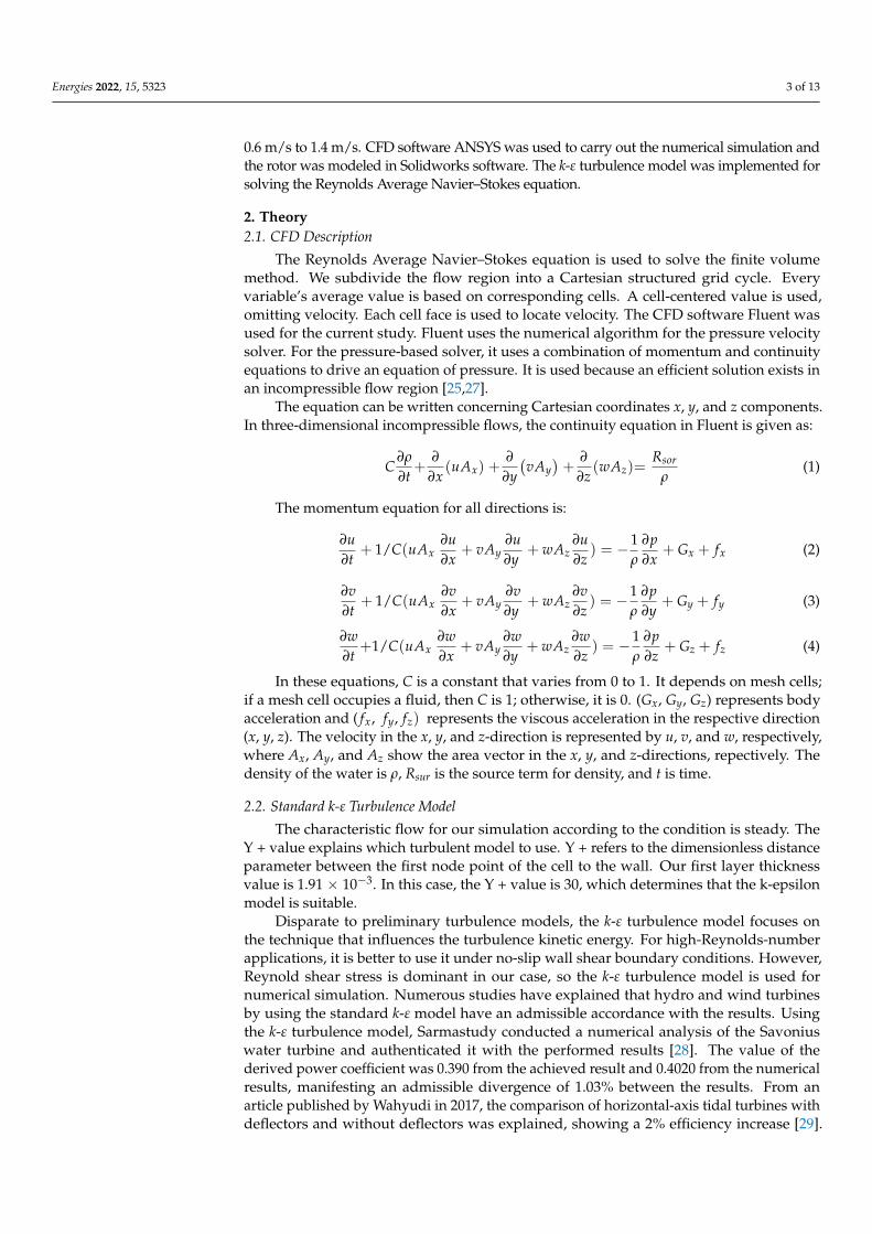
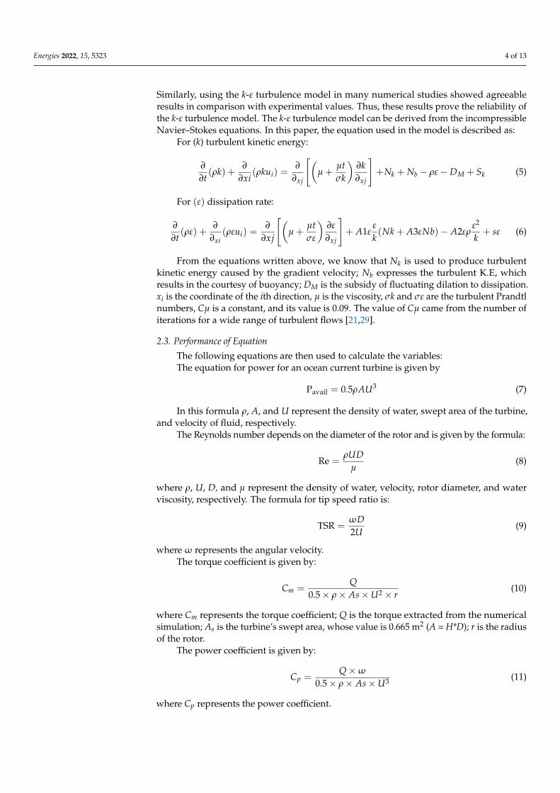
Solidworks software was used to create geometry and was then exported to AnsysFluent for numerical simulations. In this report, a horizontal-axis water turbine wasinvestigated. The collation of this paper was carried out before the simulation, whichexplains the scheme we should use [waterotor]. The first step was to regenerate geometry,and Figure 1 shows the dimensions of case 1. The outer diameter of the turbine was 0.95 m.Therefore, the diameter of the inner arc was 0.34 m and the diameter of the outer arc was0.68 m. The cylinder-like rotor had a radius of 0.175 m attached to the blade. The heightof the turbine blade was 0.7 m. The end plate of radius 0.55 m was also attached witha turbine thickness of 0.05 m. Due to the difficulty and cost of computational time, theturbine’s deflector and end plate effect will be examined in a future study. After this, thegeometry was converted into a step file and was imported into DesignModeler for furtherexplanation of the outer and inner domains. Figure 2 represents a 3D isometric view withend plates, and Figure 3 shows it without end plates.

Energies 2022, 15, x FOR PEER REVIEW 5 of 13

3. Numerical Setup 3.1. Geometry Modeling

Solidworks software was used to create geometry and was then exported to Ansys Fluent for numerical simulations. In this report, a horizontal-axis water turbine was investigated. The collation of this paper was carried out before the simulation, which explains the scheme we should use [waterotor]. The first step was to regenerate geometry, and Figure 1 shows the dimensions of case 1. The outer diameter of the turbine was 0.95 m. Therefore, the diameter of the inner arc was 0.34 m and the diameter of the outer arc was 0.68 m. The cylinder-like rotor had a radius of 0.175 m attached to the blade. The height of the turbine blade was 0.7 m. The end plate of radius 0.55 m was also attached with a turbine thickness of 0.05 m. Due to the difficulty and cost of computational time, the turbine’s deflector and end plate effect will be examined in a future study. After this, the geometry was converted into a step file and was imported into DesignModeler for further explanation of the outer and inner domains. Figure 2 represents a 3D isometric view with end plates, and Figure 3 shows it without end plates.

Figure 1. Dimensions of turbine (case 1).

Figure 2. Isometric view of the turbine (case 1).

Figure 1. Dimensions of turbine (case 1).

Energies 2022, 15, x FOR PEER REVIEW 5 of 13

3. Numerical Setup 3.1. Geometry Modeling

Solidworks software was used to create geometry and was then exported to Ansys Fluent for numerical simulations. In this report, a horizontal-axis water turbine was investigated. The collation of this paper was carried out before the simulation, which explains the scheme we should use [waterotor]. The first step was to regenerate geometry, and Figure 1 shows the dimensions of case 1. The outer diameter of the turbine was 0.95 m. Therefore, the diameter of the inner arc was 0.34 m and the diameter of the outer arc was 0.68 m. The cylinder-like rotor had a radius of 0.175 m attached to the blade. The height of the turbine blade was 0.7 m. The end plate of radius 0.55 m was also attached with a turbine thickness of 0.05 m. Due to the difficulty and cost of computational time, the turbine’s deflector and end plate effect will be examined in a future study. After this, the geometry was converted into a step file and was imported into DesignModeler for further explanation of the outer and inner domains. Figure 2 represents a 3D isometric view with end plates, and Figure 3 shows it without end plates.

Figure 1. Dimensions of turbine (case 1).

Figure 2. Isometric view of the turbine (case 1). Figure 2. Isometric view of the turbine (case 1).

Energies 2022, 15, 5323 6 of 13Energies 2022, 15, x FOR PEER REVIEW 6 of 13

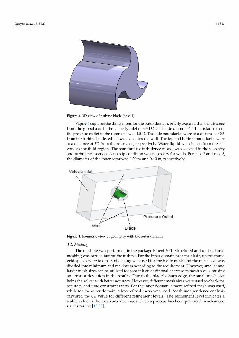
Figure 3. 3D view of turbine blade (case 1).

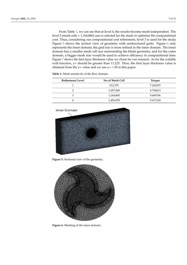
Figure 4 explains the dimensions for the outer domain, briefly explained as the distance from the global axis to the velocity inlet of 3.5 D (D is blade diameter). The distance from the pressure outlet to the rotor axis was 4.5 D. The side boundaries were at a distance of 0.5 from the turbine blade, which was considered a wall. The top and bottom boundaries were at a distance of 2D from the rotor axis, respectively. Water liquid was chosen from the cell zone as the fluid region. The standard k-ε turbulence model was selected in the viscosity and turbulence section. A no-slip condition was necessary for walls. For case 2 and case 3, the diameter of the inner rotor was 0.30 m and 0.40 m, respectively.

Figure 4. Isometric view of geometry with the outer domain.

3.2. Meshing The meshing was performed in the package Fluent 20.1. Structured and unstructured

meshing was carried out for the turbine. For the inner domain near the blade, unstructured grid spaces were taken. Body sizing was used for the blade mesh and the mesh size was divided into minimum and maximum according to the requirement. However, smaller and larger mesh sizes can be utilized to inspect if an additional decrease in mesh size is causing an error or deviation in the results. Due to the blade’s sharp edge, the small mesh size helps the solver with better accuracy. However, different mesh sizes were used to check the accuracy and time constraint ratios. For the inner domain, a more refined mesh was used, while for the outer domain, a less refined mesh was used. Mesh independence analysis captured the Cm value for different refinement levels. The refinement level indicates a stable value as the mesh size decreases. Such a process has been practiced in advanced structures too [13,30].

Figure 3. 3D view of turbine blade (case 1).

Figure 4 explains the dimensions for the outer domain, briefly explained as the distancefrom the global axis to the velocity inlet of 3.5 D (D is blade diameter). The distance fromthe pressure outlet to the rotor axis was 4.5 D. The side boundaries were at a distance of 0.5from the turbine blade, which was considered a wall. The top and bottom boundaries wereat a distance of 2D from the rotor axis, respectively. Water liquid was chosen from the cellzone as the fluid region. The standard k-ε turbulence model was selected in the viscosityand turbulence section. A no-slip condition was necessary for walls. For case 2 and case 3,the diameter of the inner rotor was 0.30 m and 0.40 m, respectively.

Energies 2022, 15, x FOR PEER REVIEW 6 of 13

Figure 3. 3D view of turbine blade (case 1).

Figure 4 explains the dimensions for the outer domain, briefly explained as the distance from the global axis to the velocity inlet of 3.5 D (D is blade diameter). The distance from the pressure outlet to the rotor axis was 4.5 D. The side boundaries were at a distance of 0.5 from the turbine blade, which was considered a wall. The top and bottom boundaries were at a distance of 2D from the rotor axis, respectively. Water liquid was chosen from the cell zone as the fluid region. The standard k-ε turbulence model was selected in the viscosity and turbulence section. A no-slip condition was necessary for walls. For case 2 and case 3, the diameter of the inner rotor was 0.30 m and 0.40 m, respectively.

Figure 4. Isometric view of geometry with the outer domain.

3.2. Meshing The meshing was performed in the package Fluent 20.1. Structured and unstructured

meshing was carried out for the turbine. For the inner domain near the blade, unstructured grid spaces were taken. Body sizing was used for the blade mesh and the mesh size was divided into minimum and maximum according to the requirement. However, smaller and larger mesh sizes can be utilized to inspect if an additional decrease in mesh size is causing an error or deviation in the results. Due to the blade’s sharp edge, the small mesh size helps the solver with better accuracy. However, different mesh sizes were used to check the accuracy and time constraint ratios. For the inner domain, a more refined mesh was used, while for the outer domain, a less refined mesh was used. Mesh independence analysis captured the Cm value for different refinement levels. The refinement level indicates a stable value as the mesh size decreases. Such a process has been practiced in advanced structures too [13,30].

Figure 4. Isometric view of geometry with the outer domain.

3.2. Meshing

The meshing was performed in the package Fluent 20.1. Structured and unstructuredmeshing was carried out for the turbine. For the inner domain near the blade, unstructuredgrid spaces were taken. Body sizing was used for the blade mesh and the mesh size wasdivided into minimum and maximum according to the requirement. However, smaller andlarger mesh sizes can be utilized to inspect if an additional decrease in mesh size is causingan error or deviation in the results. Due to the blade’s sharp edge, the small mesh sizehelps the solver with better accuracy. However, different mesh sizes were used to check theaccuracy and time constraint ratios. For the inner domain, a more refined mesh was used,while for the outer domain, a less refined mesh was used. Mesh independence analysiscaptured the Cm value for different refinement levels. The refinement level indicates astable value as the mesh size decreases. Such a process has been practiced in advancedstructures too [13,30].

Energies 2022, 15, 5323 7 of 13

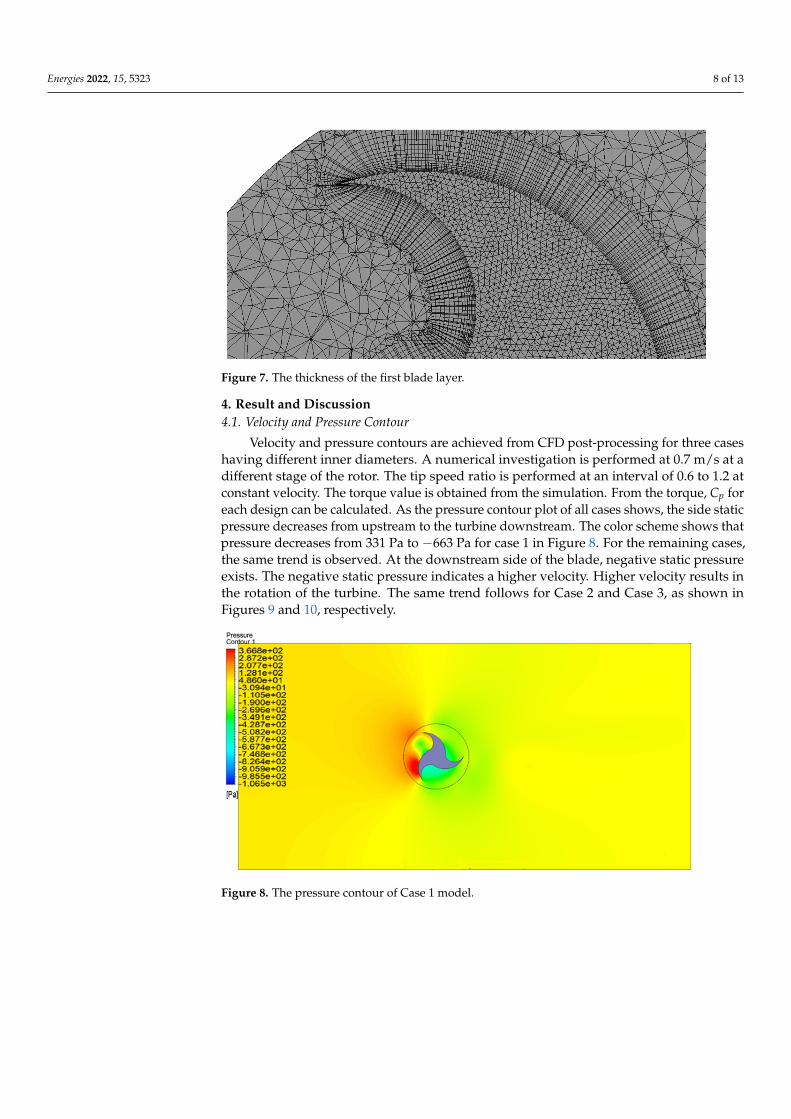
From Table 1, we can see that at level 4, the results become mesh-independent. Thelevel 3 (mesh cells = 1,164,860) case is selected for the study to optimize the computationalcost. Thus, considering our computational cost refinement, level 3 is used for the study.Figure 5 shows the section view of geometry with unstructured grids. Figure 6 onlyrepresents the inner domain; the grid size is more refined in the inner domain. The innerdomain has a smaller mesh cell size surrounding the blade geometry, and for the outerdomain, a bigger mesh size would be used to achieve efficiency in computational time.Figure 7 shows the first layer thickness value we chose for our research. As for the scalablewall function, y+ should be greater than 11.225. Thus, the first layer thickness value isobtained from the y+ value and we use y+ = 50 in this paper.

Table 1. Mesh sensitivity of the flow domain.

Refinement Level No of Mesh Cell Torque

1 912,375 7.265479

2 1,097,000 8.768413

3 1,164,860 9.669196

4 1,456,978 9.671234

Energies 2022, 15, x FOR PEER REVIEW 7 of 13

From Table 1, we can see that at level 4, the results become mesh-independent. The level 3 (mesh cells = 1,164,860) case is selected for the study to optimize the computational cost. Thus, considering our computational cost refinement, level 3 is used for the study. Figure 5 shows the section view of geometry with unstructured grids. Figure 6 only rep-resents the inner domain; the grid size is more refined in the inner domain. The inner domain has a smaller mesh cell size surrounding the blade geometry, and for the outer domain, a bigger mesh size would be used to achieve efficiency in computational time. Figure 7 shows the first layer thickness value we chose for our research. As for the scalable wall function, y+ should be greater than 11.225. Thus, the first layer thickness value is obtained from the y+ value and we use y+ =50 in this paper.

Table 1. Mesh sensitivity of the flow domain.

Refinement Level No of Mesh Cell Torque 1 912,375 7.265479 2 1,097,000 8.768413 3 1,164,860 9.669196 4 1,456,978 9.671234

Figure 5. Sectional view of the geometry.

Figure 6. Meshing of the inner domain.

Figure 5. Sectional view of the geometry.

Energies 2022, 15, x FOR PEER REVIEW 7 of 13

From Table 1, we can see that at level 4, the results become mesh-independent. The level 3 (mesh cells = 1,164,860) case is selected for the study to optimize the computational cost. Thus, considering our computational cost refinement, level 3 is used for the study. Figure 5 shows the section view of geometry with unstructured grids. Figure 6 only rep-resents the inner domain; the grid size is more refined in the inner domain. The inner domain has a smaller mesh cell size surrounding the blade geometry, and for the outer domain, a bigger mesh size would be used to achieve efficiency in computational time. Figure 7 shows the first layer thickness value we chose for our research. As for the scalable wall function, y+ should be greater than 11.225. Thus, the first layer thickness value is obtained from the y+ value and we use y+ =50 in this paper.

Table 1. Mesh sensitivity of the flow domain.

Refinement Level No of Mesh Cell Torque 1 912,375 7.265479 2 1,097,000 8.768413 3 1,164,860 9.669196 4 1,456,978 9.671234

Figure 5. Sectional view of the geometry.

Figure 6. Meshing of the inner domain. Figure 6. Meshing of the inner domain.

Energies 2022, 15, 5323 8 of 13Energies 2022, 15, x FOR PEER REVIEW 8 of 13

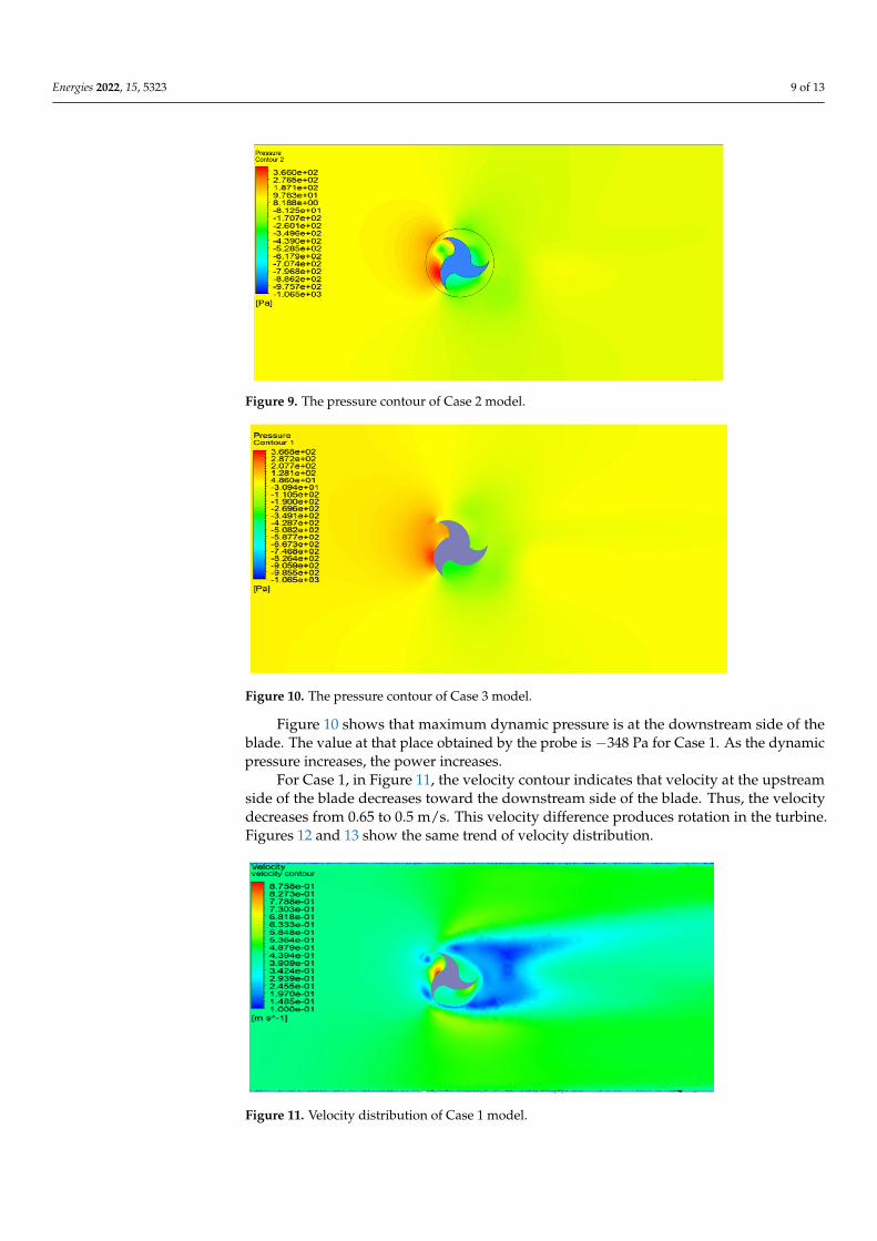
Figure 7. The thickness of the first blade layer.

4. Result and Discussion 4.1. Velocity and Pressure Contour

Velocity and pressure contours are achieved from CFD post-processing for three cases having different inner diameters. A numerical investigation is performed at 0.7 m/s at a different stage of the rotor. The tip speed ratio is performed at an interval of 0.6 to 1.2 at constant velocity. The torque value is obtained from the simulation. From the torque, Cp for each design can be calculated. As the pressure contour plot of all cases shows, the side static pressure decreases from upstream to the turbine downstream. The color scheme shows that pressure decreases from 331 Pa to −663 Pa for case 1 in Figure 8. For the re-maining cases, the same trend is observed. At the downstream side of the blade, negative static pressure exists. The negative static pressure indicates a higher velocity. Higher ve-locity results in the rotation of the turbine. The same trend follows for Case 2 and Case 3, as shown in Figures 9 and 10, respectively.

Figure 8. The pressure contour of Case 1 model.

Figure 7. The thickness of the first blade layer.

4. Result and Discussion4.1. Velocity and Pressure Contour

Velocity and pressure contours are achieved from CFD post-processing for three caseshaving different inner diameters. A numerical investigation is performed at 0.7 m/s at adifferent stage of the rotor. The tip speed ratio is performed at an interval of 0.6 to 1.2 atconstant velocity. The torque value is obtained from the simulation. From the torque, Cp foreach design can be calculated. As the pressure contour plot of all cases shows, the side staticpressure decreases from upstream to the turbine downstream. The color scheme shows thatpressure decreases from 331 Pa to −663 Pa for case 1 in Figure 8. For the remaining cases,the same trend is observed. At the downstream side of the blade, negative static pressureexists. The negative static pressure indicates a higher velocity. Higher velocity results inthe rotation of the turbine. The same trend follows for Case 2 and Case 3, as shown inFigures 9 and 10, respectively.

Energies 2022, 15, x FOR PEER REVIEW 8 of 13

Figure 7. The thickness of the first blade layer.

4. Result and Discussion 4.1. Velocity and Pressure Contour

Velocity and pressure contours are achieved from CFD post-processing for three cases having different inner diameters. A numerical investigation is performed at 0.7 m/s at a different stage of the rotor. The tip speed ratio is performed at an interval of 0.6 to 1.2 at constant velocity. The torque value is obtained from the simulation. From the torque, Cp for each design can be calculated. As the pressure contour plot of all cases shows, the side static pressure decreases from upstream to the turbine downstream. The color scheme shows that pressure decreases from 331 Pa to −663 Pa for case 1 in Figure 8. For the re-maining cases, the same trend is observed. At the downstream side of the blade, negative static pressure exists. The negative static pressure indicates a higher velocity. Higher ve-locity results in the rotation of the turbine. The same trend follows for Case 2 and Case 3, as shown in Figures 9 and 10, respectively.

Figure 8. The pressure contour of Case 1 model. Figure 8. The pressure contour of Case 1 model.

Energies 2022, 15, 5323 9 of 13Energies 2022, 15, x FOR PEER REVIEW 9 of 13

Figure 9. The pressure contour of Case 2 model.

Figure 10. The pressure contour of Case 3 model.

Figure 10 shows that maximum dynamic pressure is at the downstream side of the blade. The value at that place obtained by the probe is −348 Pa for Case 1. As the dynamic pressure increases, the power increases.

For Case 1, in Figure 11, the velocity contour indicates that velocity at the upstream side of the blade decreases toward the downstream side of the blade. Thus, the velocity decreases from 0.65 to 0.5 m/s. This velocity difference produces rotation in the turbine. Figures 12 and 13 show the same trend of velocity distribution.

Figure 11. Velocity distribution of Case 1 model.

Figure 9. The pressure contour of Case 2 model.

Energies 2022, 15, x FOR PEER REVIEW 9 of 13

Figure 9. The pressure contour of Case 2 model.

Figure 10. The pressure contour of Case 3 model.

Figure 10 shows that maximum dynamic pressure is at the downstream side of the blade. The value at that place obtained by the probe is −348 Pa for Case 1. As the dynamic pressure increases, the power increases.

For Case 1, in Figure 11, the velocity contour indicates that velocity at the upstream side of the blade decreases toward the downstream side of the blade. Thus, the velocity decreases from 0.65 to 0.5 m/s. This velocity difference produces rotation in the turbine. Figures 12 and 13 show the same trend of velocity distribution.

Figure 11. Velocity distribution of Case 1 model.

Figure 10. The pressure contour of Case 3 model.

Figure 10 shows that maximum dynamic pressure is at the downstream side of theblade. The value at that place obtained by the probe is −348 Pa for Case 1. As the dynamicpressure increases, the power increases.

For Case 1, in Figure 11, the velocity contour indicates that velocity at the upstreamside of the blade decreases toward the downstream side of the blade. Thus, the velocitydecreases from 0.65 to 0.5 m/s. This velocity difference produces rotation in the turbine.Figures 12 and 13 show the same trend of velocity distribution.

Energies 2022, 15, x FOR PEER REVIEW 9 of 13

Figure 9. The pressure contour of Case 2 model.

Figure 10. The pressure contour of Case 3 model.

Figure 10 shows that maximum dynamic pressure is at the downstream side of the blade. The value at that place obtained by the probe is −348 Pa for Case 1. As the dynamic pressure increases, the power increases.

For Case 1, in Figure 11, the velocity contour indicates that velocity at the upstream side of the blade decreases toward the downstream side of the blade. Thus, the velocity decreases from 0.65 to 0.5 m/s. This velocity difference produces rotation in the turbine. Figures 12 and 13 show the same trend of velocity distribution.

Figure 11. Velocity distribution of Case 1 model.

Figure 11. Velocity distribution of Case 1 model.

Energies 2022, 15, 5323 10 of 13Energies 2022, 15, x FOR PEER REVIEW 10 of 13

Figure 12. Velocity distribution of Case 2 model.

Figure 13. Velocity distribution of Case 3 model.

Therefore, with the increase in the intersection, the velocity magnitude difference on both sides of the turbine decreases gradually to ensure lift generation for the turbine. For all cases, the same trend follows.

4.2. Comparison of Torque and Power Curve The performance equation is used for calculating the torque and power coefficients

for all cases. Through formulation, we find the angular velocity at different tip speed ra-tios (0.6–1.2) at a constant velocity of 0.7 m/s. The findings are compared with published results [21]. We obtain the power coefficient after analysis. After validation, we change the inner diameter to improve the efficiency from the angular velocity, torque, and power coefficient for all cases, as shown in Tables 1 and 2.

Table 2. Values of Tip Speed Ratios (TSRs) and Angular Velocity at constant stream velocity.

Velocity (m/s) Tip Speed Ratio

(TSR) Angular Velocity

(Rad/s) 0.7 0.6 0.885 0.7 0.8 1.17 0.7 1 1.474 0.7 1.2 1.768

Figure 12. Velocity distribution of Case 2 model.

Energies 2022, 15, x FOR PEER REVIEW 10 of 13

Figure 12. Velocity distribution of Case 2 model.

Figure 13. Velocity distribution of Case 3 model.

Therefore, with the increase in the intersection, the velocity magnitude difference on both sides of the turbine decreases gradually to ensure lift generation for the turbine. For all cases, the same trend follows.

4.2. Comparison of Torque and Power Curve The performance equation is used for calculating the torque and power coefficients

for all cases. Through formulation, we find the angular velocity at different tip speed ra-tios (0.6–1.2) at a constant velocity of 0.7 m/s. The findings are compared with published results [21]. We obtain the power coefficient after analysis. After validation, we change the inner diameter to improve the efficiency from the angular velocity, torque, and power coefficient for all cases, as shown in Tables 1 and 2.

Table 2. Values of Tip Speed Ratios (TSRs) and Angular Velocity at constant stream velocity.

Velocity (m/s) Tip Speed Ratio

(TSR) Angular Velocity

(Rad/s) 0.7 0.6 0.885 0.7 0.8 1.17 0.7 1 1.474 0.7 1.2 1.768

Figure 13. Velocity distribution of Case 3 model.

Therefore, with the increase in the intersection, the velocity magnitude difference onboth sides of the turbine decreases gradually to ensure lift generation for the turbine. Forall cases, the same trend follows.

4.2. Comparison of Torque and Power Curve

The performance equation is used for calculating the torque and power coefficientsfor all cases. Through formulation, we find the angular velocity at different tip speedratios (0.6–1.2) at a constant velocity of 0.7 m/s. The findings are compared with publishedresults [21]. We obtain the power coefficient after analysis. After validation, we changethe inner diameter to improve the efficiency from the angular velocity, torque, and powercoefficient for all cases, as shown in Tables 1 and 2.

Table 2. Values of Tip Speed Ratios (TSRs) and Angular Velocity at constant stream velocity.

Velocity (m/s) Tip Speed Ratio(TSR)

Angular Velocity(Rad/s)

0.7 0.6 0.885

0.7 0.8 1.17

0.7 1 1.474

0.7 1.2 1.768

Figure 14 shows the relationship of iteration with torque values for case 1. After278 iterations, a straight path is followed by the torque curve, due to which convergence

Energies 2022, 15, 5323 11 of 13

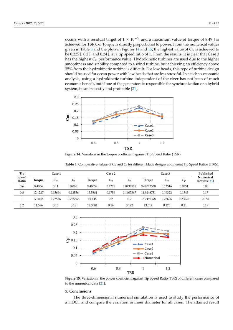
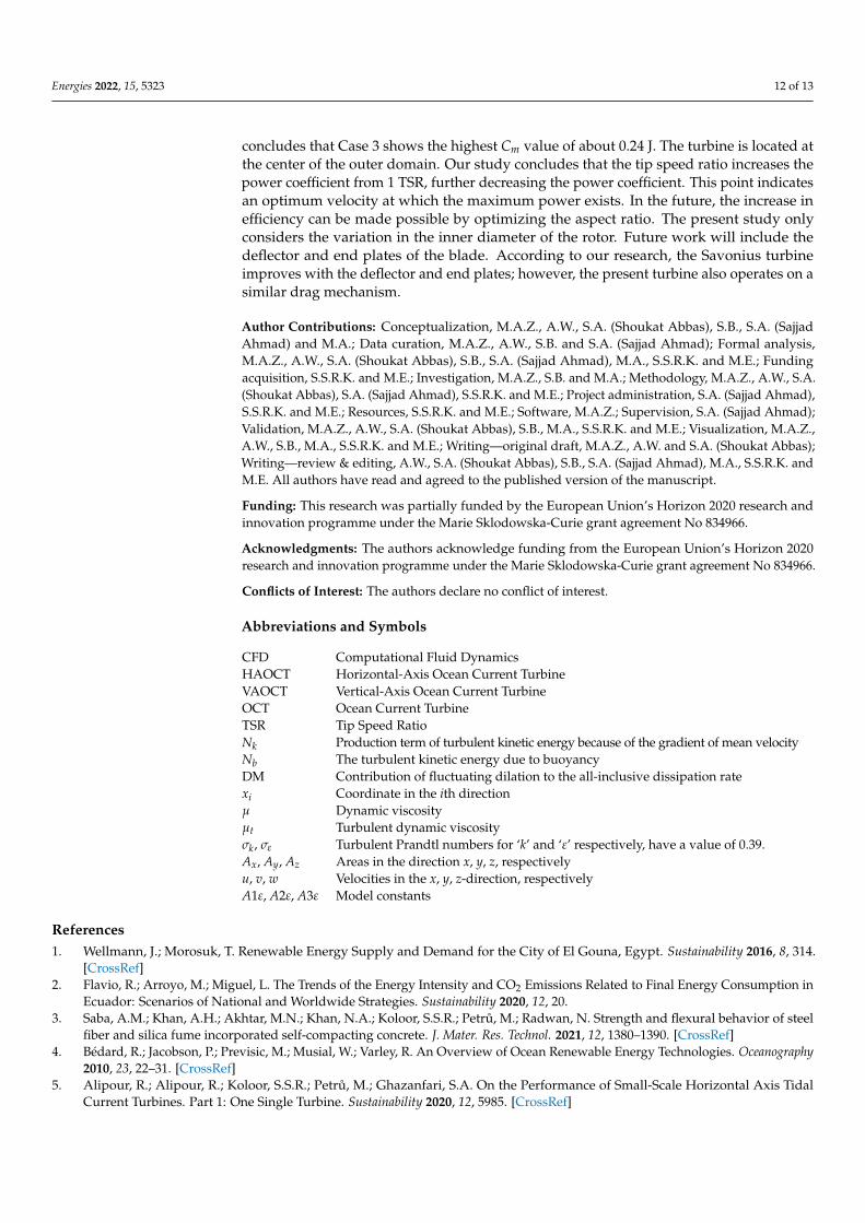
occurs with a residual target of 1 × 10−3, and a maximum value of torque of 8.49 J isachieved for TSR 0.6. Torque is directly proportional to power. From the numerical valuesgiven in Table 3 and the plots in Figures 14 and 15, the highest value of Cm is achieved tobe 0.225 J, 0.2 J, and 0.24 J, at a tip speed ratio of 1. From the results, it is clear that Case 3has the highest Cm performance value. Hydrokinetic turbines are used due to the highersmoothness and stability compared to a wind turbine, but achieving an efficiency above35% from the hydrokinetic turbine is difficult. For low heads, this type of turbine designshould be used for ocean power with low heads that are less stressful. In a techno-economicanalysis, using a hydrokinetic turbine independent of the river has not been of mucheconomic benefit, but if one of the generators is responsible for synchronization or a hybridsystem, it can be costly and profitable [21].

Energies 2022, 15, x FOR PEER REVIEW 11 of 13

Figure 14 shows the relationship of iteration with torque values for case 1. After 278 iterations, a straight path is followed by the torque curve, due to which convergence occurs with a residual target of 1 × 10−3, and a maximum value of torque of 8.49 J is achieved for TSR 0.6. Torque is directly proportional to power. From the numerical values given in Table 3 and the plots in Figures 14 and 15, the highest value of Cm is achieved to be 0.225 J, 0.2 J, and 0.24 J, at a tip speed ratio of 1. From the results, it is clear that Case 3 has the highest Cm performance value. Hydrokinetic turbines are used due to the higher smoothness and stability compared to a wind turbine, but achieving an efficiency above 35% from the hydrokinetic turbine is difficult. For low heads, this type of turbine design should be used for ocean power with low heads that are less stressful. In a techno-economic analysis, using a hydrokinetic turbine independent of the river has not been of much economic benefit, but if one of the generators is responsible for synchronization or a hybrid system, it can be costly and profitable [21].

Table 3. Comparative values of Cm and Cp for different blade designs at different Tip Speed Ratios (TSRs).

Tip Speed Ratio

Case 1 Case 2 Case 3 Published Numerical Results [21] Torque Cm Cp Torque Cm Cp Torque Cm Cp

0.6 8.4964 0.11 0.066 9.48659 0.1228 0.0736918 9.66793538 0.12516 0.0751 0.08 0.8 12.1227 0.15694 0.12556 13.5881 0.1759 0.1407367 14.9248751 0.19322 0.1545 0.17 1 17.4458 0.22586 0.225866 15.448 0.2 0.2 18.2490398 0.23626 0.23626 0.185

1.2 11.586 0.15 0.18 12.3584 0.16 0.192 13.517 0.175 0.21 0.17

Figure 14. Variation in the torque coefficient against Tip Speed Ratio (TSR).

Figure 15. Variation in the power coefficient against Tip Speed Ratio (TSR) of different cases com-pared to the numerical data [21].

0

0.05

0.1

0.15

0.2

0.25

0.3

0.6 0.8 1 1.2

Cm

TSR

Case1Case2Case3

0

0.05

0.1

0.15

0.2

0.25

0.3

0.6 0.8 1 1.2

Cp

TSR

Case1Case2Case3Numerical [16]

Figure 14. Variation in the torque coefficient against Tip Speed Ratio (TSR).

Table 3. Comparative values of Cm and Cp for different blade designs at different Tip Speed Ratios (TSRs).

TipSpeedRatio

Case 1 Case 2 Case 3 PublishedNumericalResults [21]Torque Cm Cp Torque Cm Cp Torque Cm Cp

0.6 8.4964 0.11 0.066 9.48659 0.1228 0.0736918 9.66793538 0.12516 0.0751 0.08

0.8 12.1227 0.15694 0.12556 13.5881 0.1759 0.1407367 14.9248751 0.19322 0.1545 0.17

1 17.4458 0.22586 0.225866 15.448 0.2 0.2 18.2490398 0.23626 0.23626 0.185

1.2 11.586 0.15 0.18 12.3584 0.16 0.192 13.517 0.175 0.21 0.17

Energies 2022, 15, x FOR PEER REVIEW 11 of 13

Figure 14 shows the relationship of iteration with torque values for case 1. After 278 iterations, a straight path is followed by the torque curve, due to which convergence occurs with a residual target of 1 × 10−3, and a maximum value of torque of 8.49 J is achieved for TSR 0.6. Torque is directly proportional to power. From the numerical values given in Table 3 and the plots in Figures 14 and 15, the highest value of Cm is achieved to be 0.225 J, 0.2 J, and 0.24 J, at a tip speed ratio of 1. From the results, it is clear that Case 3 has the highest Cm performance value. Hydrokinetic turbines are used due to the higher smoothness and stability compared to a wind turbine, but achieving an efficiency above 35% from the hydrokinetic turbine is difficult. For low heads, this type of turbine design should be used for ocean power with low heads that are less stressful. In a techno-economic analysis, using a hydrokinetic turbine independent of the river has not been of much economic benefit, but if one of the generators is responsible for synchronization or a hybrid system, it can be costly and profitable [21].

Table 3. Comparative values of Cm and Cp for different blade designs at different Tip Speed Ratios (TSRs).

Tip Speed Ratio

Case 1 Case 2 Case 3 Published Numerical Results [21] Torque Cm Cp Torque Cm Cp Torque Cm Cp

0.6 8.4964 0.11 0.066 9.48659 0.1228 0.0736918 9.66793538 0.12516 0.0751 0.08 0.8 12.1227 0.15694 0.12556 13.5881 0.1759 0.1407367 14.9248751 0.19322 0.1545 0.17 1 17.4458 0.22586 0.225866 15.448 0.2 0.2 18.2490398 0.23626 0.23626 0.185

1.2 11.586 0.15 0.18 12.3584 0.16 0.192 13.517 0.175 0.21 0.17

Figure 14. Variation in the torque coefficient against Tip Speed Ratio (TSR).

Figure 15. Variation in the power coefficient against Tip Speed Ratio (TSR) of different cases com-pared to the numerical data [21].

0

0.05

0.1

0.15

0.2

0.25

0.3

0.6 0.8 1 1.2

Cm

TSR

Case1Case2Case3

0

0.05

0.1

0.15

0.2

0.25

0.3

0.6 0.8 1 1.2

Cp

TSR

Case1Case2Case3Numerical [16]

Figure 15. Variation in the power coefficient against Tip Speed Ratio (TSR) of different cases comparedto the numerical data [21].

5. Conclusions

The three-dimensional numerical simulation is used to study the performance ofa HOCT and compare the variation in inner diameter for all cases. The attained result

Energies 2022, 15, 5323 12 of 13

concludes that Case 3 shows the highest Cm value of about 0.24 J. The turbine is located atthe center of the outer domain. Our study concludes that the tip speed ratio increases thepower coefficient from 1 TSR, further decreasing the power coefficient. This point indicatesan optimum velocity at which the maximum power exists. In the future, the increase inefficiency can be made possible by optimizing the aspect ratio. The present study onlyconsiders the variation in the inner diameter of the rotor. Future work will include thedeflector and end plates of the blade. According to our research, the Savonius turbineimproves with the deflector and end plates; however, the present turbine also operates on asimilar drag mechanism.

Author Contributions: Conceptualization, M.A.Z., A.W., S.A. (Shoukat Abbas), S.B., S.A. (SajjadAhmad) and M.A.; Data curation, M.A.Z., A.W., S.B. and S.A. (Sajjad Ahmad); Formal analysis,M.A.Z., A.W., S.A. (Shoukat Abbas), S.B., S.A. (Sajjad Ahmad), M.A., S.S.R.K. and M.E.; Fundingacquisition, S.S.R.K. and M.E.; Investigation, M.A.Z., S.B. and M.A.; Methodology, M.A.Z., A.W., S.A.(Shoukat Abbas), S.A. (Sajjad Ahmad), S.S.R.K. and M.E.; Project administration, S.A. (Sajjad Ahmad),S.S.R.K. and M.E.; Resources, S.S.R.K. and M.E.; Software, M.A.Z.; Supervision, S.A. (Sajjad Ahmad);Validation, M.A.Z., A.W., S.A. (Shoukat Abbas), S.B., M.A., S.S.R.K. and M.E.; Visualization, M.A.Z.,A.W., S.B., M.A., S.S.R.K. and M.E.; Writing—original draft, M.A.Z., A.W. and S.A. (Shoukat Abbas);Writing—review & editing, A.W., S.A. (Shoukat Abbas), S.B., S.A. (Sajjad Ahmad), M.A., S.S.R.K. andM.E. All authors have read and agreed to the published version of the manuscript.

Funding: This research was partially funded by the European Union’s Horizon 2020 research andinnovation programme under the Marie Sklodowska-Curie grant agreement No 834966.

Acknowledgments: The authors acknowledge funding from the European Union’s Horizon 2020research and innovation programme under the Marie Sklodowska-Curie grant agreement No 834966.

Conflicts of Interest: The authors declare no conflict of interest.

Abbreviations and Symbols

CFD Computational Fluid DynamicsHAOCT Horizontal-Axis Ocean Current TurbineVAOCT Vertical-Axis Ocean Current TurbineOCT Ocean Current TurbineTSR Tip Speed RatioNk Production term of turbulent kinetic energy because of the gradient of mean velocityNb The turbulent kinetic energy due to buoyancyDM Contribution of fluctuating dilation to the all-inclusive dissipation ratexi Coordinate in the ith directionµ Dynamic viscosityµt Turbulent dynamic viscosityσk, σε Turbulent Prandtl numbers for ‘k’ and ‘ε’ respectively, have a value of 0.39.Ax, Ay, Az Areas in the direction x, y, z, respectivelyu, v, w Velocities in the x, y, z-direction, respectivelyA1ε, A2ε, A3ε Model constants

References1. Wellmann, J.; Morosuk, T. Renewable Energy Supply and Demand for the City of El Gouna, Egypt. Sustainability 2016, 8, 314.

[CrossRef]2. Flavio, R.; Arroyo, M.; Miguel, L. The Trends of the Energy Intensity and CO2 Emissions Related to Final Energy Consumption in

Ecuador: Scenarios of National and Worldwide Strategies. Sustainability 2020, 12, 20.3. Saba, A.M.; Khan, A.H.; Akhtar, M.N.; Khan, N.A.; Koloor, S.S.R.; Petru, M.; Radwan, N. Strength and flexural behavior of steel

fiber and silica fume incorporated self-compacting concrete. J. Mater. Res. Technol. 2021, 12, 1380–1390. [CrossRef]4. Bédard, R.; Jacobson, P.; Previsic, M.; Musial, W.; Varley, R. An Overview of Ocean Renewable Energy Technologies. Oceanography

2010, 23, 22–31. [CrossRef]5. Alipour, R.; Alipour, R.; Koloor, S.S.R.; Petru, M.; Ghazanfari, S.A. On the Performance of Small-Scale Horizontal Axis Tidal

Current Turbines. Part 1: One Single Turbine. Sustainability 2020, 12, 5985. [CrossRef]

Energies 2022, 15, 5323 13 of 13

6. Nachtane, T.; Moumen, S. Design and Hydrodynamic Performance of a Horizontal Axis Hydrokinetic Turbine. Int. J. Automot.Mech. Eng. 2019, 16, 6453–6469. [CrossRef]

7. Lestari, H.; Arentsen, M.; Bressers, H.; Gunawan, B.; Iskandar, J. Parikesit Sustainability of Renewable Off-Grid Technology forRural Electrification: A Comparative Study Using the IAD Framework. Sustainability 2018, 10, 4512. [CrossRef]

8. Magagna, D.; Uihlein, A. Ocean energy development in Europe: Current status and future perspectives. Int. J. Mar. Energy 2015,11, 84–104. [CrossRef]

9. Alipour, R.; Alipout, R.; Fardian, F.; Kollor, S.; Petru, M. Performance improvement of a new proposed Savonius hydrokineticturbine: A numerical investigation. Energy Rep. 2020, 6, 3051–3066. [CrossRef]

10. Le Traon, P.; Morrow, R. Ocean currents and eddies. In International Geophysics; Elsevier: Amsterdam, The Netherlands, 2001; pp. 171–215.11. Hu, S.; Sprintall, J.; Guan, C.; McPhaden, M.; Wang, F.; Hu, D.; Cai, W. Deep-reaching acceleration of global mean ocean circulation

over the past two decades. Sci. Adv. 2020, 6, eaax7727. [CrossRef]12. Farokhi Nejad, A.; Alipour, R.; Shokri Rad, M.; Yazid Yahya, M.; Rahimian Koloor, S.S.; Petru, M. Using Finite Element Approach

for Crashworthiness Assessment of a Polymeric Auxetic Structure Subjected to the Axial Loading. Polymers 2020, 12, 1312.[CrossRef] [PubMed]

13. Kashyzadeh, K.; Koloor, S.R.; Bidgoli, M.O.; Petru, M.; Asfarjani, A.A. An Optimum Fatigue Design of Polymer Composite-Compressed Natural Gas Tank Using Hybrid Finite Element-Response Surface Methods. Polymers 2021, 13, 483. [CrossRef][PubMed]

14. Flajser, S.H.; Kash, D.E.; White, I.L.; Bergey, K.H.; Chartock, M.A.; Devine, M.D.; Salomon, S.N.; Young, H.W. Energy under theOceans: A Technology Assessment of Outer Continental Shelf Oil and Gas Operations. Technol. Cult. 1975, 16, 122. [CrossRef]

15. Laws, N.D.; Epps, B.P. Hydrokinetic energy conversion: Technology, research, and outlook. Renew. Sustain. Energy Rev. 2016, 57,1245–1259. [CrossRef]

16. Fraenkel, P.L. Marine current turbines: Pioneering the development of marine kinetic energy converters. Proc. Inst. Mech. Eng.Part A J. Power Energy 2007, 221, 159–169. [CrossRef]

17. Tian, W.; Mao, Z.; Ding, H. Design, test and numerical simulation of a low-speed horizontal axis hydrokinetic turbine. Int. J. Nav.Arch. Ocean Eng. 2018, 10, 782–793. [CrossRef]

18. Khan, M.; Bhuyan, G.; Iqbal, M.; Quaicoe, J. Hydrokinetic energy conversion systems and assessment of horizontal and verticalaxis turbines for river and tidal applications: A technology status review. Appl. Energy 2009, 86, 1823–1835. [CrossRef]

19. Khan, M.; Iqbal, M.; Quaicoe, J. River current energy conversion systems: Progress, prospects and challenges. Renew. Sustain.Energy Rev. 2008, 12, 2177–2193. [CrossRef]

20. Chen, L.; Chen, J.; Zhang, Z. Review of the Savonius rotor’s blade profile and its performance. J. Renew. Sustain. Energy 2018, 10, 013306.[CrossRef]

21. Maldar, N.R.; Ng, C.Y.; Ean, L.W.; Oguz, E.; Fitriadhy, A.; Kang, H.S. A Comparative Study on the Performance of a HorizontalAxis Ocean Current Turbine Considering Deflector and Operating Depths. Sustainability 2020, 12, 3333. [CrossRef]

22. Zakaria, A.; Ibrahim, M. Numerical Performance Evaluation of Savonius Rotors by Flow-driven and Sliding-mesh Approaches.Int. J. Adv. Trends Comput. Sci. Eng. 2019, 8, 57–61.

23. Asterita, T.J. Available online: www.waterotor.com (accessed on 20 December 2021).24. Golecha, K.; Eldho, T.; Prabhu, S. Influence of the deflector plate on the performance of modified Savonius water turbine. Appl.

Energy 2011, 88, 3207–3217. [CrossRef]25. Sahim, K.; Ihtisan, K.; Santoso, D.; Sipahutar, R. Experimental Study of Darrieus-Savonius Water Turbine with Deflector: Effect of

Deflector on the Performance. Int. J. Rotating Mach. 2014, 2014, 203108. [CrossRef]26. Hemida, M.; Abdel-Fadeel, W.A.; Ramadan, A.; Aissa, W. Numerical Investigation of hydrokinetic Savonius rotor with two

shielding plates. Appl. Model. Simul. 2019, 3, 85–94.27. Kolekar, N.; Banerjee, A. Performance characterization and placement of a marine hydrokinetic turbine in a tidal channel under

boundary proximity and blockage effects. Appl. Energy 2015, 148, 121–133. [CrossRef]28. Sarma, N.; Biswas, A.; Misra, R. Experimental and computational evaluation of Savonius hydrokinetic turbine for low velocity

condition with comparison to Savonius wind turbine at the same input power. Energy Convers. Manag. 2014, 83, 88–98. [CrossRef]29. Wahyudi, B.; Adiwidodo, S. The influence of moving deflector angle to positive torque on the hydrokinetic cross flow savonius

vertical axis turbine. Int. Energy J. 2017, 17, 11–22.30. Koloor, S.S.R.; Karimzadeh, A.; Tamin, M.N.; Shukor, M.H.A. Effects of Sample and Indenter Configurations of Nanoindentation

Experiment on the Mechanical Behavior and Properties of Ductile Materials. Metals 2018, 8, 421. [CrossRef]