Costly horizontal differentiation

��

��

��

��

��

�� !�� !�� !�� !�� " �#" �#" �#" �# ��$��$��$��$��

��%&� �' ��(()��%&� �' ��(()��%&� �' ��(()��%&� �' ��(()

Costly horizontal differentiation?

Joao Correia-da-Silva

CEF.UP and Faculdade de Economia. Universidade do Porto.

Joana Pinho

Faculdade de Economia. Universidade do Porto.

November 4th, 2009

Abstract. We study the effect of quadratic differentiation costs in the Hotelling model

of endogenous product differentiation. The equilibrium location choices are found to

depend on the magnitude of the differentiation costs (relatively to the transportation

costs supported by consumers). When the differentiation costs are low, there is maximum

differentiation. When they are intermediate, there is partial differentiation, with a degree

of differentiation that decreases with the differentiation costs. When they are above

a certain threshold, there is no equilibrium. In any case, the socially optimal degree

of differentiation is always lower than the equilibrium level. We also study the case

of collusion between firms. If firms can combine locations but not prices, they locate

asymmetrically when differentiation costs are high and choose maximum differentiation

when they are low. When collusion extends to price setting, there is partial differentiation.

Keywords: Costly product differentiation, Spatial competition, Hotelling model.

JEL Classification Numbers: D43, L13, R32.

?Joao Correia-da-Silva ([email protected]) acknowledges support from CEF.UP, Fundacao para a Ciencia eTecnologia and FEDER (research grant PTDC/ECO/66186/2006). Joana Pinho ([email protected])acknowledges support from Fundacao para a Ciencia e Tecnologia (Ph.D. scholarship).

1

1 Introduction

In many markets, firms horizontally differentiate their products, making them more at-

tractive to some consumers and less attractive to others. Having their own preferred

variety, consumers become less sensitive to price variations. This relaxes competition,

allowing firms to increase their profits.

In order to differentiate their products, firms may have to carry out costly activities, like

advertising or product design. Such differentiation costs have been overlooked in most

of the theoretical literature.1 We contribute to fill this gap, by studying the effects of

differentiation costs in a duopoly model with endogenous horizontal differentiation.

The standard model of horizontal differentiation is due to Hotelling (1929). In this model,

there are two firms that choose their locations in a linear city, and then engage in price

competition to sell their products. Consumers, who are spread along the linear city, choose

which of the products to buy, taking into account, besides prices, the transportation cost

that they support. Such transportation costs are most frequently assumed to be linear or

quadratic (d’Aspremont, Gabszewicz and Thisse, 1979).

We study an extension of this model that considers quadratic differentiation costs (Mat-

sushima, 2004). More precisely, it is considered that the marginal cost of production

increases with the square of the distance between the firm and the center of the linear

city. This additional cost may be interpreted as resulting from the process of modify-

ing a standard product, as in the work of Eaton and Schmitt (1994), or as the cost of

transporting inputs bought from suppliers that are located at the center of the city.

The model of Matsushima (2004) is more general, comprising two suppliers located arbi-

trarily.2 Our setup corresponds to the particular case in which the suppliers are located

at the center. Such location may be optimal for suppliers that serve many industries

spread along the city.3 On the other hand, Matsushima (2004) restricts his analysis to

1A notable exception is the work of Eaton and Schmitt (1994), who consider firms that produce anendogenous number of varieties which may be more or less costly to produce, according to whether theirspecifications are distant from or close to the specifications of a ‘basic product’.

2Matsushima (2004) also studies the (endogenous) location of suppliers. See also the related work ofKourandi and Vettas (2009).

3If the firms need to buy inputs from many suppliers, uniformly dispersed along the city, then thecost of transporting these inputs also increases with the distance between the firm and the center. Thisprovides further justification for our assumption.

2

the case in which the differentiation costs (supported by firms) are lower than the trans-

portation costs (supported by consumers). Removing this assumption, we obtain several

new results.

A framework that is also similar to ours was proposed by Aiura and Sato (2008). They

consider that the differentiation costs are linear and that firms can locate outside the city.

These two assumptions are different from ours and lead to different results. Still, they

conclude, as we do, that the location of the firms depends on the relationship between

the differentiation costs and the transportation costs.4

In the classical model (d’Aspremont, Gabszewicz and Thisse, 1979), which does not in-

clude differentiation costs, firms choose to locate at the extremes of the linear city in

order to soften price competition. In our setup, the differentiation costs increase the at-

tractiveness of the central locations, as the production cost increases with the distance to

the center. This generates richer equilibrium possibilities.

We find that low differentiation costs, relatively to the transportation costs, do not affect

the equilibrium location choices of the firms (maximum differentiation). However, suffi-

ciently high differentiation costs induce firms to locate in the interior of the city (partial

differentiation), increasingly closer to the center as the differentiation costs increase. We

obtain, in this way, a relationship between the magnitude of differentiation costs and the

degree of differentiation. We also find that extremely high differentiation costs imply the

non-existence of equilibrium location choices.5

The socially optimal locations are found to correspond to partial differentiation, with a

degree of differentiation that is decreasing with the differentiation costs. In the absence

of differentiation costs, firms locate in the midpoints between the center and the extremes

(a known result). As the differentiation costs increase, firms locate closer and closer

4The model of Gupta, Kats and Pal (1994) is farther from ours. They consider a monopolist sup-plier, while we assume a competitive input industry. Moreover, they allow for the existence of severaldownstream firms and consider that the (linear) transportation costs are supported by the firms. An-other alternative setup was considered by Brekke and Straume (2004), who assumed a bilateral monopolyrelationship between upstream and downstream firms.

5More precisely, we consider that the transportation costs supported by a consumer located at x whobuys from a firm located at a are t (x− a)2 and that the differentiation cost supported by a firm locatedat a is τ

(12 − a

)2. We find that maximum differentiation is the unique equilibrium if τt ≤

12 , that partial

differentiation is the unique equilibrium if 12 <

τt ≤

192 , and that there is no equilibrium if τ

t >192 . We

complement, thus, the results of Matsushima (2004), as he restricted his analysis to the case in whichτt ≤ 1 and did not establish uniqueness of equilibrium.

3

to the center, converging to a situation of no differentiation. Comparing the optimal

locations with the competitive equilibrium ones, we conclude that the socially optimal

degree of differentiation is always lower than the degree of differentiation that is induced

by competition.6

Finally, we study the case of collusive behavior between firms. In the case of partial

collusion, in which firms can combine locations but not prices, we obtain a rather sur-

prising result. If differentiation costs are high, one of the firms locates at an extreme,

while the other locates between this same extreme and the center (if differentiation costs

are low, firms agree on maximum differentiation). When collusion is full (extends to the

price setting stage), firms locate: in the midpoints between the center and the extremes,

if differentiation costs are lower than transportation costs; and increasingly closer to the

center, as the differentiation costs increase above this threshold.

The remainder of the article is organized as follows. In Section 2, we setup the model and

introduce notation. In Sections 3, 4 and 5, we fully characterize the relationship between

the degree of differentiation and the cost of differentiation, in three economic scenarios:

competition (Section 3), social planning (Section 4), and collusion (Section 5). Section 6

concludes the article with some remarks.

2 The Model

There are two firms, 1 and 2, and a continuum of consumers homogeneously distributed

on the unit interval, [0, 1]. In a first stage, firms simultaneously choose their location

(which is interpreted as their product specification) on the unit interval. The location of

firm 1 is denoted a, and the location of firm 2 is denoted 1− b. In the second stage, firms

simultaneously choose the prices to charge for their goods, p1 and p2.

As the model of Aiura and Sato (2008), firms located farther from the center have higher

production costs. This may be interpreted as the cost of modifying a standard product,

or as the cost of transporting inputs bought from suppliers that are located at the center

6We remark that the model at hands considers that the demand is inelastic and that prices have aneutral effect on social welfare. This should be kept in mind for an adequate interpretation of the welfareimplications of the model.

4

of the city. The marginal cost of firm 1 is τ(

12− a)2

and the marginal cost of firm 2 is

τ(

12− b)2

, with τ ≥ 0.7

Each consumer chooses whether to buy the product of firm 1 or the product of firm

2. Consumers are heterogeneous in their tastes, preferring products located near them.

Assuming that such transportation costs are also quadratic, the total cost of buying goods

1 and 2, supported by a consumer located at x, are p1 + t(x− a)2 and p2 + t(x− 1 + b)2,

respectively, with t > 0.8

It is straightforward to determine the indifferent consumer (valid for a+ b < 1):

x =1 + a− b

2+

p2 − p1

2t(1− a− b), (1)

which corresponds to the demand for the product sold by firm 1. The demand for the

product sold by firm 2 is: 1− x = 1−a+b2

+ p1−p22t(1−a−b) .

3 Competitive equilibrium locations

We start by studying the competitive scenario. In the first stage, firms simultaneously

choose their location on the unit interval. In the second stage, firms simultaneously choose

the prices to charge for their goods.

The profit of firm 1, as a function of locations and prices, is:9

Π1 =

[p1 − τ

(1

2− a)2][

1 + a− b2

+p2 − p1

2t(1− a− b)

]. (2)

7The difference with respect to the model of Aiura and Sato (2008) is that here marginal costs increasequadratically instead of linearly with the distance to the center.

8The model that we are considering corresponds to the model proposed by Matsushima (2004) withsuppliers located at the center. But we do not restrict the analysis to the case in which τ ≤ t.

9This expression is valid for a + b < 1. It can be shown that if firms choose the same location(a+ b = 1), then the equilibrium prices are equal to marginal cost, p1 = τ

(12 − a

)2 and p2 = τ(

12 − b

)2,and, therefore, the resulting profits are null.

5

Profit maximization by firm 1 implies that:

p1 =1

2

[t− a2t− 2bt+ b2t+ p2 + τ

(1

2− a)2]. (3)

Analogously, the price set by firm 2 is:

p2 =1

2

[t− b2t− 2at+ a2t+ p1 + τ

(1

2− b)2]. (4)

From the best response functions, (3) and (4), we obtain the prices that the firms choose,

as a function of their locations:

p1(a, b) = t− 2

3at− 1

3a2t− 4

3bt+

1

3b2t+

2τ

3

(1

2− a)2

+τ

3

(1

2− b)2

, (5)

p2(a, b) = t− 2

3bt− 1

3b2t− 4

3at+

1

3a2t+

2τ

3

(1

2− b)2

+τ

3

(1

2− a)2

. (6)

Given these prices, the indifferent consumer is located at:

x(a, b) =3 + a− b

6+τ

t

(12− b)2 −

(12− a)2

6 (1− a− b)=

1

2+

1 + τt

6(a− b) .

And the profit obtained by firm 1 is:

Π1(a, b) =t

18(1− a− b)

[3 + (a− b)

(1 +

τ

t

)]2

. (7)

Observe that, given the ratio τt, the value of t is irrelevant for the behavior of firms (the

constant t18

could be ignored in the maximization problem).

Definition 1.

A profile of locations, (a∗, b∗), is an equilibrium if and only if:

(i) a∗ ∈ arg maxa∈[0,1]

{Π1(a, b∗)};

(ii) b∗ ∈ arg maxb∈[0,1]

{Π2(a∗, b)}.

6

When the differentiation costs are low relatively to the transportation costs, there is

maximum differentiation (firms locate at the extremes of the unit interval).

Proposition 1.

Maximum differentiation, (a∗, b∗) = (0, 0), is an equilibrium if and only if:10

τ

t≤ 1

2.

On the other hand, we find that no differentiation cannot be an equilibrium (firms never

locate simultaneously at the center).

Proposition 2.

No differentiation, (a∗, b∗) =(

12, 1

2

), is never an equilibrium.

For moderately high values of the differentiation cost (relatively to the transportation

cost), there is partial differentiation. Firms locate in the interior of the unit interval, at

the same distance from the center.

Proposition 3.

Partial differentiation, (a∗, b∗) = (dc, dc), with dc ∈ (0, 12), is an equilibrium if and only if:

1

2<τ

t≤ 19

2and dc =

1

2− 3/4

1 + τt

.

Observe that as τt

increases, the firms locate closer and closer to the center. When τt

= 192

,

we have dc = 37' 0.43. This is as close to the center as they get (locating in the center

would imply null profits for both firms).

Finally, we find that asymmetric differentiation is never an equilibrium.

Proposition 4.

Asymmetric differentiation, (a∗, b∗) = (da, db), with da 6= db, is never an equilibrium.

10All the proofs are collected in the Appendix.

7

We have completely characterized the equilibria of the model, which is always unique:

there is maximum differentiation if τt≤ 1

2, and partial differentiation if 1

2< τ

t≤ 19

2(with

the degree of differentiation being symmetric and increasing with τt). For τ

t> 19

2, there

is no equilibrium.

Firms face a trade-off between increasing differentiation to reduce competition in the price

setting stage and decreasing differentiation to lower their production costs. If differentia-

tion costs are low, relatively to transportation costs, the market power effect dominates.

There is maximum differentiation. If differentiation costs are above a certain threshold,

the trade-off becomes relevant. Firms locate in the interior of the city (partial differentia-

tion), increasingly closer to the center as the differentiation costs increase. We are able to

relate, in this way, the magnitude of differentiation costs and the degree of differentiation.

4 Socially optimal locations

Consider now that a social planner decides locations and prices with the objective of

maximizing social welfare, which is defined as the sum of the consumers’ surplus with the

profits of the firms.

Since all consumers find it optimal to buy one unit of the good (from one of the firms or

the other), and since the price paid is a transference (does not affect social welfare), maxi-

mizing social welfare is equivalent to minimizing the sum of the consumers’ transportation

costs with the firms’ differentiation costs.

Total transportation costs, supported by consumers, are given by:

Lt (a, b, x) =

∫ x

0

t(x− a)2dx+

∫ 1

x

t(x− 1 + b)2dx =

= t

[(1− a− b) x2 +

(a2 − b2 + 2b− 1

)x+ b2 − b+

1

3

].

And the differentiation costs, supported by the firms, are:

Lτ (a, b, x) = τ

[(1

2− a)2

x+

(1

2− b)2

(1− x)

].

8

The social planner chooses the locations of the firms (a and b) and the prices of the goods

(which, then, determine x) with the objective of maximizing:

W (a, b, x) = −t[(1− a− b) x2 +

(a2 − b2 + 2b− 1

)x+ b2 − b+

1

3

]−

−τ

[(1

2− a)2

x+

(1

2− b)2

(1− x)

]. (8)

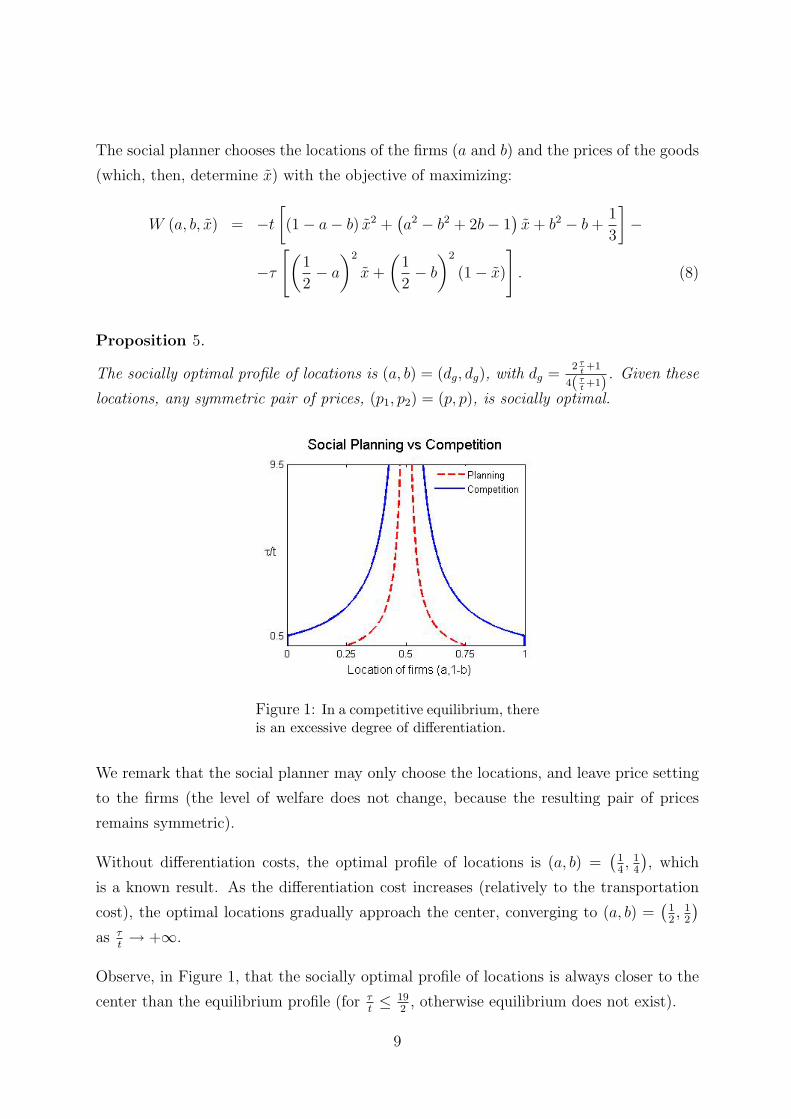
Proposition 5.

The socially optimal profile of locations is (a, b) = (dg, dg), with dg =2 τt

+1

4( τt +1). Given these

locations, any symmetric pair of prices, (p1, p2) = (p, p), is socially optimal.

Figure 1: In a competitive equilibrium, thereis an excessive degree of differentiation.

We remark that the social planner may only choose the locations, and leave price setting

to the firms (the level of welfare does not change, because the resulting pair of prices

remains symmetric).

Without differentiation costs, the optimal profile of locations is (a, b) =(

14, 1

4

), which

is a known result. As the differentiation cost increases (relatively to the transportation

cost), the optimal locations gradually approach the center, converging to (a, b) =(

12, 1

2

)as τ

t→ +∞.

Observe, in Figure 1, that the socially optimal profile of locations is always closer to the

center than the equilibrium profile (for τt≤ 19

2, otherwise equilibrium does not exist).

9

5 Collusive locations

5.1 Partial collusion

We now study the case in which firms collude when making their (irreversible) location

decisions. We start by assuming that firms can commit on their location choices, but not

on the prices to set afterwards. Therefore, price-setting remains competitive.11

Alternatively, we can assume that firms are also able to commit on the prices to set, but

that collusive price setting would be detected and punished by anti-trust authorities.

Firms jointly choose their locations, (a, b), with the objective of maximizing the sum of

their profits, which is given by:12

Πpj (a, b) =t

9(1− a− b)

[9 + (a− b)2

(1 +

τ

t

)2]

We find that for relatively low differentiation costs, firms decide to locate at the extremes

(maximum differentiation). For sufficiently high differentiation costs, firms decide to

locate asymmetrically: one at an extreme, and the other between this same extreme and

the center.

Proposition 6.

The collusive location decision (with subsequent price competition) is:13

(i) maximum differentiation, (a∗, b∗) = (0, 0), if τt≤ 5;

(ii) asymmetric differentiation, (a∗, b∗) = (0, dpj) or (a∗, b∗) = (dpj, 0), if τt≥ 5,

with dpj = 13

+ 13

√1− 27

(1 + τ

t

)−2.

When the differentiation cost reaches a certain threshold, τt

= 5, the optimal location

11Friedman and Thisse (1993) study an infinitely repeated game version of the Hotelling model, inwhich locations are chosen (once and for all) in period 0 and prices are chosen in each period. In sucha model, collusion in the price setting stage can be sustainable. In our one-shot game, collusive pricesetting requires the ability to make a commitment.

12Since we are assuming that firms compete in prices, the profit of firm 1 is still given by (7). Analo-gously, the expression for the profit of firm 2 is: Π2 (a, b) = t

18 (1− a− b)[3 + (b− a)

(1 + τ

t

)]2.13When τ

t = 5, decisions (i) and (ii) are equally optimal.

10

jumps from (a∗, b∗) = (0, 0) to (a∗, b∗) =(0, 1

2

). The benefit of reducing differentiation

costs becomes dominant relatively to the benefit of reducing competition in the price

setting stage. The optimal compromise is to have one firm in the center, minimizing the

differentiation costs, and another in an extreme, providing sufficient differentiation.

As the ratio between the differentiation cost and the transportation cost parameters in-

creases from 5 to +∞, one of the firms remains located at an extreme, while the other

moves from the center (dpj = 12) towards its competitor (dpj = 2

3). It is somewhat para-

doxical that this firm becomes farther from the center, increasing differentiation costs,

and closer to the competitor, increasing competition in the price setting stage. But this

movement actually decreases the total differentiation costs, as the firm which is near the

center increases its market share.14

5.2 Full collusion

To study the case of full collusion, in which collusion extends to price-setting, we need to

consider a reservation utility for the consumers (otherwise firms would be able to increase

prices to infinity).

Let the utility of a consumer located at x that buys the good from firm i be ui(x) =

V − pi − t (x− di)2, where V is the money equivalent of the satisfaction provided by the

good, pi is the price paid for the good and di is the location of firm i. If the consumer

does not buy the good, her utility is null, u0(x) = 0.

To guarantee full market coverage, we assume that V ≥ 5t4

+ τ4.15

Lemma 1.

In the fully collusive scenario, when V ≥ 5t4

+ τ4, firms choose locations and prices which

induce all consumers to buy the good (full market coverage).

The fully collusive location choices correspond to partial differentiation. Firms locate: in

the midpoints between the center and the extremes, if differentiation costs are lower than

14This asymmetric solution should be associated with a side-payment from the firm which locates nearthe center to the firm which locates at the extreme.

15The corresponding assumption made by Friedman and Thisse (1993), in their dynamic model withoutdifferentiation costs, was V ≥ 3t.

11

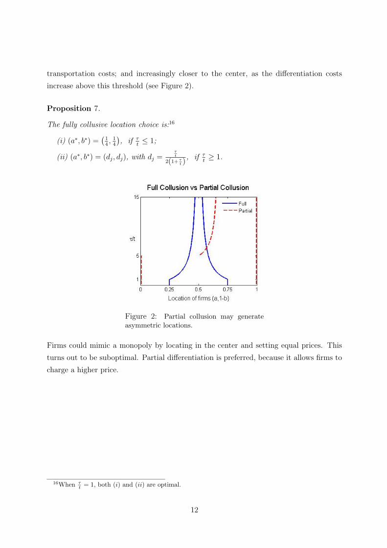
transportation costs; and increasingly closer to the center, as the differentiation costs

increase above this threshold (see Figure 2).

Proposition 7.

The fully collusive location choice is:16

(i) (a∗, b∗) =(

14, 1

4

), if τ

t≤ 1;

(ii) (a∗, b∗) = (dj, dj), with dj =τt

2(1+ τt )

, if τt≥ 1.

Figure 2: Partial collusion may generateasymmetric locations.

Firms could mimic a monopoly by locating in the center and setting equal prices. This

turns out to be suboptimal. Partial differentiation is preferred, because it allows firms to

charge a higher price.

16When τt = 1, both (i) and (ii) are optimal.

12

6 Conclusion

We have shown how the existence of quadratic differentiation costs affects the degree

of differentiation, in the context of the Hotelling duopoly model. According to whether

the Hotelling line is interpreted as the set of possible locations in space or as the set of

possible product characteristics, the differentiation cost can be interpreted as the cost of

transporting raw materials from the center of a linear city or as the cost of transforming

a standard product into a differentiated variety.

We have considered three different economic scenarios: competition, social planning and

collusion. In any case, the location choices only depend on the ratio between the differ-

entiation cost (incurred by firms) and the transportation cost (supported by consumers)

parameters, τ/t. Firms locate symmetrically and closer to the center as τ/t increases,

except in the case of partial collusion. If firms can collude on locations but not on prices

and τ/t is high enough, then they choose to locate on the same side of the market.

Our model helps in understanding the choice of a costly degree of differentiation. Firms

take into account not only the increase in market power that results from a unique po-

sitioning but also the cost of acquiring such a privileged situation, for example, through

advertising or design. This trade-off generates a new effect of exogenous shocks: the degree

of differentiation may increase or decrease as a result of variations in the transportation

cost. In the standard model, maximum differentiation was robust to such perturbations.

13

7 Appendix

Proof of Proposition 1: From the definition of equilibrium, it follows that maximal

differentiation, (a∗, b∗) = (0, 0), is an equilibrium if and only if:

(i) 0 ∈ arg maxa∈[0,1]

{Π1(a, 0)};

(ii) 0 ∈ arg maxb∈[0,1]

{Π2(0, b)}.

By symmetry, to prove that (a∗, b∗) = (0, 0) is an equilibrium, it is enough to check that

(i) is true.

When b = 0, we have:

Π1(a, 0) =t

18(1− a)

[3 + a

(1 +

τ

t

)]2

. (9)

The derivative of the profit function with respect to location is:

∂Π1(a, 0)

∂a=

t

18

(3 + a+ a

τ

t

)(−1− 3a+ 2

τ

t− 3a

τ

t

).

The signal of ∂Π1(a,0)∂a

is equal to the signal of 2 τt−1−3

(1 + τ

t

)a. It is clear that if ∂Π1(a,0)

∂a

is negative at a = 0, then it is negative for any a ∈ [0, 1).

Therefore, the necessary and sufficient condition for maximal differentiation to be an

equilibrium isτ

t≤ 1

2. �

Proof of Proposition 2: No differentiation, (a∗, b∗) = (1/2, 1/2), is an equilibrium if

and only if:

(i)1

2∈ arg max

a∈[0,1]{Π1 (a, 1/2)};

(ii)1

2∈ arg max

b∈[0,1]{Π2 (1/2, b)}.

By symmetry, to show that no differentiation is an equilibrium, it is only necessary to

show that:1

2∈ arg max

a∈[0, 12 ]{Π1 (a, 1/2)}.

14

When b = 12, the profit of firm 1 is:

Π1(a, 1/2) =t

18

(1

2− a)(

5

2+ a+ a

τ

t− τ

2t

)2

.

Calculating the derivative with respect to location, we obtain:

∂Π1(a, 1/2)

∂a=

t

18

(5

2+ a+ a

τ

t− τ

2t

)(−3

2− 3a− 3a

τ

t+

3τ

2t

).

A necessary condition for no differentiation to be an equilibrium is that this derivative is

positive as a→ 12

−. But we find that it is always negative:

lima→ 1

2

−

∂Π1(a, 1/2)

∂a= − t

2.

�

Proof of Proposition 3: Partial differentiation, (a∗, b∗) = (dc, dc), with dc ∈ (0, 1/2), is

an equilibrium if and only if:

(i) dc ∈ arg maxa∈[0,1]

{Π1(a, dc)};

(ii) dc ∈ arg maxb∈[0,1]

{Π2(dc, b)}.

With b = dc, the profit obtained by firm 1 is:

Π1(a, dc) =t

18(1− a− dc)

[3 + (a− dc)

(1 +

τ

t

)]2

. (10)

The partial derivative with respect to a is:

∂Π1(a, dc)

∂a=

t

18

[3 + (a− dc)

(1 +

τ

t

)](−1− 3a− dc + 2

τ

t− 3a

τ

t− dcτ

t

).

For the first-order condition of (i) to hold, we must have:

∂Π1(a, dc)

∂a

∣∣∣∣a=dc

= 0 ⇔ dc =2 τt− 1

4 τt

+ 4.

15

Notice that dc ∈ (0, 1/2) if and only if τt> 1

2. Therefore, partial differentiation can only

be an equilibrium for τt> 1

2.

To check the second-order condition, write the second derivative of the profit function

with respect to location:

∂2Π1(a, dc)

∂a2=t

9

(1 +

τ

t

)(−5− 3a+ dc +

τ

t− 3a

τ

t+ dc

τ

t

).

The local second order condition always holds:

∂2Π1(a, dc)

∂a2

∣∣∣∣a=dc

=t

9

(1 +

τ

t

)(−5− 2dc +

τ

t− 2dc

τ

t

)= − t

2

(1 +

τ

t

).

The global second order condition may not hold, but there is a threshold, a0 > dc, such

that ∂2Π1(a,dc)∂a2 is negative (positive) for a > a0 (a < a0):

∂2Π1

∂a2(a, dc) ≤ 0⇔ a ≥ a0 =

1

2−

94

1 + τt

.

For τt≤ 7

2, we have a0 ≤ 0, which means that the global second order condition holds.

Thus, for τt∈ (1/2, 7/2], partial differentiation is an equilibrium.

For higher values of τt, we must compare Π1(dc, dc) with Π1(0, dc) (since Π1 is convex for

a < a0, the only other candidate for a maximizer is a = 0). With a = d, the profit of firm

1 is:

Π1 (dc, dc) =t

2(1− 2dc) =

t

2

[1−

2 τt− 1

2(1 + τ

t

)] =3t

4(1 + τ

t

) .If firm 1 decides to locate at the extreme, a = 0, its profit is:

Π1(0, dc) =3t

4(1 + τ

t

) [ 1

864

(5 + 2

τ

t

)(13− 2

τ

t

)2].

16

For partial differentiation to be an equilibrium, we must have:

Π1(0, dc) ≤ Π1 (dc, dc)⇔1

864

(5 + 2

τ

t

)(13− 2

τ

t

)2

≤ 1 ⇔ 8(τt

)3

− 84(τt

)2

+ 78τ

t− 19 ≤ 0.

This occurs if and only ifτ

t≤ 19

2. �

Proof of Proposition 4: Asymmetric differentiation, (a∗, b∗) = (da, db), with da 6= db,

is an equilibrium if and only if:

(i) da ∈ arg maxa∈[0,1]

{Π1(a, db)};

(ii) db ∈ arg maxb∈[0,1]

{Π2(da, b)}.

Without loss of generality, suppose that da 6= 0. From the proof of Proposition 3, we

know that the location b which maximizes the profit of firm 2 is either b = 0 or b = da.

Therefore, the only candidate for an asymmetric equilibrium is (a∗, b∗) = (da, 0).

With b = 0, we have (9):

Π1(a, 0) =t

18(1− a)

[3 + a

(1 +

τ

t

)]2

.

A necessary condition for (a∗, b∗) = (da, 0) to be an equilibrium is that:

∂Π1(a, 0)

∂a

∣∣∣∣a=da

= 0⇔ t

18

(3 + da +

τ

tda

)(−1− 3da + 2

τ

t− 3da

τ

t

)= 0.

Which is equivalent to:

da =2 τt− 1

3(τt

+ 1) . (11)

Another necessary condition for (a∗, b∗) = (da, 0) to be an equilibrium is that:

∂Π2(da, b)

∂b

∣∣∣∣b=0

= 0.

17

By symmetry, this condition is equivalent to:

∂Π1(a, da)

∂a

∣∣∣∣a=0

= 0 ⇔ t

18

[3− da

(1 +

τ

t

)](−1− da + 2

τ

t− τ

td)

= 0.

Solving in order to da, we obtain:

da =3

1 + τt

or da =2 τt− 1

τt

+ 1.

The second possibility is incompatible with (11), therefore, we must have:

da =3

1 + τt

=2 τt− 1

3(τt

+ 1) ⇔ {

da = 12,

τt

= 5.

With τt

= 5, the local second order condition for b = 0 to be a maximizer of Π2(1/2, b) is

equivalent to:

∂2Π1

∂a2(a, 1/2)

∣∣∣∣a=0

≤ 0 ⇔ −5 +1

2+ 5 +

5

2≤ 0,

which does not hold. �

Proof of Proposition 5: The derivative of W with respect to x is:

∂W

∂x= −t(x− a)2 + t(x− 1 + b)2 − τ

[(1

2− a)2

−(

1

2− b)2].

The corresponding first-order condition, ∂W∂x

= 0, can be written as:

2atx− ta2 − 2t (1− b) x+ t (1− b)2 = τ

[(1

2− a)2

−(

1

2− b)2]⇔

⇔ x =

τt

[(12− a)2 −

(12− b)2]

+ a2 − (1− b)2

−2 (1− a− b)⇔

⇔ x =τt

[a2 − a− b2 + b]− (1− a− b) (a− b+ 1)

−2 (1− a− b)⇔

⇔ x =1

2+a− b

2

(1 +

τ

t

). (12)

18

Welfare is concave in x, as the second derivative is:

∂2W

∂x2= −2t (1− a− b) ≤ 0.

The first-order condition with respect to a, ∂W∂a

= 0, is equivalent to:

x (τ − 2aτ − 2at+ tx) = 0 ⇔ x = 0 ∨ x = 2a+τ

t(2a− 1) . (13)

Similarly, the first-order condition with respect to b is:

(x− 1) (2bτ − t− τ + 2bt+ tx) = 0 ⇔ x = 1 ∨ x = 1− 2b+τ

t(1− 2b) . (14)

With x = 0 (the same would result for x = 1), social welfare is:

W (a, b, 0) = −t(b2 − b+

1

3

)− τ

(1

2− b)2

,

which is maximal at b = 12, attaining the value:

W

(a,

1

2, 0

)= − t

12.

For x 6= 0, from the first-order conditions, (12), (13) and (14), we obtain:

a = b = dg =2 τt

+ 1

4(1 + τ

t

) and x =1

2.

To make sure that this pair of locations is optimal, we now construct the Hessian matrix:

H (a, b, x) =

∂2W∂a2

∂2W∂a∂b

∂2W∂a∂x

∂2W∂b∂a

∂2W∂b2

∂2W∂b∂x

∂2W∂x∂a

∂2W∂x∂b

∂2W∂x2

=

=

−2x (τ + t) 0 τ − 2a(τ + t) + 2tx

0 −2 (1− x) (τ + t) 2b(τ + t)− 2t (1− x)− ττ − 2a(τ + t) + 2tx 2b(τ + t)− 2t (1− x)− τ −2t (1− a− b)

.

19

At (a, b, x) =

(2 τt

+1

4(1+ τt ),

2 τt

+1

4(1+ τt ), 1

2

)≡(dg, dg,

12

), we obtain:

H

(dg, dg,

1

2

)=

− (τ + t) 0 1

2

0 − (τ + t) −12

12

−12

− t2

τ+t

.

The local second-order condition for(dg, dg,

12

)to be a maximum is: |A1| < 0, |A2| > 0

and |A3| < 0. We have:

(i) |A1| = − (τ + t) < 0;

(ii) |A2| = det

[− (τ + t) 0

0 − (τ + t)

]= (τ + t)2 > 0;

(iii) |A3| = det

− (τ + t) 0 1

2

0 − (τ + t) −12

12

−12

− t2

τ+t

= − t2(τ+t)2

< 0.

Thus,(dg, dg,

12

)is a local maximum of W . Since the domain of W , D × [0, 1], is a

compact and W is C∞, to show that it is a global maximum, we only need to prove that

W(dg, dg,

12

)is higher than W at the frontier.17

Calculating welfare at(dg, dg,

12

), we obtain:

W

(dg, dg,

1

2

)= − 4τ + t

48(1 + τ

t

) = −t(1 + 4 τ

t

)12(4 + 4 τ

t

) > − t

12,

which is higher than welfare for x = 0.

By symmetry, the only remaining candidate is of the form (0, b, x).

But, at a = 0, ∂W∂a

> 0, therefore, (0, b, x) cannot be a maximizer. �

Proof of Proposition 6: The first-order conditions for the maximization of the joint

profit are:{∂Πpj∂a

= 0∂Πpj∂b

= 0⇔

{9 + (a− b)2 (1 + τ

t

)2= 2 (1− a− b) (a− b)

(1 + τ

t

)2,

9 + (a− b)2 (1 + τt

)2= 2 (1− a− b) (b− a)

(1 + τ

t

)2.

17The compact domain is D × [0, 1], where D ={

(a, b) ∈ [0, 1]2 : a+ b ≤ 1}

.

20

Subtracting the second from the first, we obtain a = b (which does not satisfy any of

the conditions) or a + b = 1 (which is surely not optimal, as it implies that Πj = 0).

Therefore, there are no interior maxima.

Since Πpj (a, b) is a continuous function defined on a compact domain, it has a global

maximum.18 The only possible maximizers are the frontier points with a = 0 or b = 0.

Without loss of generality, consider a = 0. The joint profit becomes:

Πpj (0, b) =t

9(1− b)

[9 + b2

(1 +

τ

t

)2].

The first-order condition of the maximization with respect to b can be written as:

2b− 3b2 =9(

1 + τt

)2 ⇔ b = dpj =1

3+

1

3

√1− 27

(1 +

τ

t

)−2

.

Therefore, only b = dpj or the frontier point b = 0 can maximize Πpj (0, b).

Accordingly, firms choose (a∗, b∗) = (0, dpj) if Πpj (0, dpj) > Πpj (0, 0), that is, if:

t

9(1− dpj)

[9 + d2

pj

(1 +

τ

t

)2]> t ⇔ τ

t> 5.

And choose (a∗, b∗) = (0, 0) otherwise, that is, when τt< 5. �

Proof of Lemma 1: Recall that u1 (x) and u2 (x) is the utility of the consumer located

at x when she buys the good from firm 1 and from firm 2, respectively.

We start by showing that the firms are always interested in selling to the consumers who

are located between them (x ∈ [a, 1− b]). Suppose, without loss of generality, that a < 12,

and, by way of contradiction, that there exists y ∈ [a, 1− b] such that u1 (y) < 0 and

u2 (y) < 0. There exists y1 ∈ (a, y) such that u1(y1) = 0. Of course that the consumers

in (y1, y) do not buy from any firm. Then, by locating at a + ε, with ε ∈ (0, y − y1),

and keeping p1 fixed, firm 1 increases its profit, by lowering the differentiation costs while

18The compact domain is D ={

(a, b) ∈ [0, 1]2 : a+ b ≤ 1}

.

21

maintaining (at least) its demand. The profit of firm 2 is not affected, thus we have a

contradiction.

We now proceed to show that the extremes of the market are also covered. By way of

contradiction, let us now suppose that there exists x1 ∈ (0, a) such that u1 (x1) = 0 and

u2 (x1) ≤ 0. Of course that the consumers located at [ 0, x1 ) do not buy from any firm. If

a > 12, by moving firm 1 to a− ε, the joint profit would increase. With a ≤ 1

2, moving to

a− ε increases demand (prices are kept fixed) but also increases the differentiation costs.

With x2 denoting the greatest x such that u2(x) ≥ 0, the joint profit is:

Πj =

[p1 − τ

(1

2− a)2]

(x− x1) +

[p2 − τ

(1

2− b)2]

(x2 − x) .

Since u1 (x1) = 0, we must have p1 = V − t (a− x1)2. And, as before, the indifferent

consumer is given by x = 1+a−b2

+ p2−p12t(1−a−b) .

The derivative of Πj with respect to x1 is:

∂Πj

∂x1

= (x− x1)∂p1

∂x1

+

[p1 − τ

(1

2− a)2]∂ (x− x1)

∂x1

,

where:

∂p1

∂x1

= 2t (a− x1) and∂ (x− x1)

∂x1

=x1 − a

1− a− b− 1 < −1.

Thus:

∂Πj

∂x1

< 2t (a− x1) (x− x1)− V + t (a− x1)2 + τ

(1

2− a)2

<

< t− V +t

4+τ

4.

Therefore, V ≥ 5t4

+ τ4

implies that ∂ΠJ∂x1

< 0. Under this assumption, joint profit maxi-

mization implies full market coverage. �

Proof of Proposition 7: Observe that if the consumers at the extremes, x = 0 and

x = 1, and the indifferent consumer, x = x, buy the good, then all the other consumers

22

also buy the good.

With a single firm producing, say firm 1, the maximum profit would be obtained by

locating the firm in the center and setting p = V − t4

(which implies u1(0) = u1(1) = 0).

The resulting profit would also be equal to V − t4. The same outcome results if both firms

locate at the center and charge this same price.

If the two firms produce, there is full market coverage if and only if u1(0) ≥ 0, u2(1) ≥ 0

and u1(x) ≥ 0.

We start by maximizing the joint profit subject to u1(0) ≥ 0 and u2(1) ≥ 0, ignoring

the restriction u(x) ≥ 0. Then, we check whether the solution obtained satisfies this

restriction. If it does, then it is the solution to our problem.

For the consumer located at x = 0 to buy the good from firm 1, the price charged, p1,

cannot be higher than V − ta2. The corresponding margin of firm 1 is: p1 − V − ta2 −τ(

12− a)2

. The highest possible margin is obtained when (the derivative with respect to

a is null):

−2ta− 2τa+ τ = 0 ⇔ a∗ =τt

2(1 + τ

t

) .To maximize its margin subject to covering x = 1, firm 2 should locate symmetrically

and set the same price. Firms are, with these decisions, maximizing their margins. If the

market is fully covered (that is, the ignored restriction is satisfied), then the joint profit

is being maximized. This occurs if the firm is closer to the center than to the extreme:

τt

2(1 + τ

t

) ≥ 1

4⇔ τ

t≥ 1.

For τt≥ 1, we have obtained the solution. Firms locate at (a∗, b∗) = (dj, dj), with

dj =τt

2(1+ τt )

, set prices p∗1 = p∗2 = V −t ( τt )2

4(1+ τt )

2 , and obtain a joint profit Πj = V − t4

( τt )2− τt

(1+ τt )

2

(higher than V − t4).

For τt< 1, the solution of the relaxed problem, obtained above, does not satisfy the

ignored restriction, u1(x) ≥ 0, where x ∈ (0, 1) as both firms are supposedly producing.

Suppose, by way of contradiction, that the solution for this case is such that u1(x) = 0,

23

u1(0) > 0 and u2(1) ≥ 0. These conditions imply that the indifferent consumer is between

both firms, a < x < 1 − b. Observe also that u1(0) ≥ u1(x) implies a < x2, and that

u2(1) ≥ u2(x) implies b ≤ 1−x2

. Therefore, a+ b ≤ 12.

But, then, the joint profit is not being maximized. It can be higher if firm 1 moves to

a+ε (towards the center) and increases p1 for the indifferent consumer to be kept constant

(revenues increase, and the differentiation costs decrease). This contradiction implies that

the solution must be such that u(x) = 0, u(0) = 0 and u(1) = 0, implying that a+ b = 12.

Since u (0) = u (1) = 0, the charged prices must be p1 = V − ta2 and p2 = V − tb2, and

the demands of firm 1 and 2 are 2a and 2b, respectively. The resulting joint profit is:

Πj = 2a

[V − ta2 − τ

(1

2− a)2]

+ 2b

[V − tb2 − τ

(1

2− b)2]

=

= 2a

[V − ta2 − τ

(1

2− a)2]

+ (1− 2a)

[V − t

(1

2− a)2

− τa2

]=

= V − 1

4t− 1

2aτ − 3a2t+ a2τ +

3

2at

The corresponding first-order condition is:

dΠj

da= 0 ⇔ 1

2(4a− 1) (τ − 3t) = 0 ⇔ a =

1

4,

because we are asuming that τt< 1.

Consequently, if τt< 1, firms choose to locate at (a∗, b∗) =

(14, 1

4

). The joint-profit, in this

case, is V − t+τ16

(higher than V − t4). �

24

References

Aiura, H. and Sato, Y. (2008), “Welfare properties of spatial competition with location-

dependent costs”, Regional Science and Urban Economics, 38, pp. 32-48.

Brekke K.R. and Straume, O.R. (2004), “Bilateral monopolies and location choice”, Re-

gional Science and Urban Economics, 34, pp. 275-288.

D’Aspremont, C., Gabszewicz, J.J. and Thisse, J.-F.(1979), “On Hotelling’s “Stability in

competition””, Econometrica, 47, pp. 1145-1150.

Eaton, B.C. and Schmitt, N. (1994), “Flexible Manufacturing and Market Structure”,

American Economic Review, 84, pp. 875-88.

Friedman, J.W. and Thisse, J.-F. (1993), “Partial collusion fosters minimum product

differentiation”, RAND Journal of Economics, 24, pp. 631-645.

Gupta, B., Kats, A. and Pal, D. (1994), “Upstream monopoly, downstream competition

and spatial price discrimination,” Regional Science and Urban Economics, 24, pp. 529-

542.

Hotelling, H. (1929), “Stability in competition”, Economic Journal, 39, pp. 41-57.

Kourandi, F. and Vettas, N. (2009), “Endogenous Spatial Differentiation with Vertical

Contracting”, mimeo.

Matsushima, N. (2004), “Technology of upstream firms and equilibrium product differen-

tiation”, International Journal of Industrial Organization, 22, pp. 1091-1114.

25

Recent FEP Working Papers

��

��

�� !�� !��"�#��

��"�#��$��%�� &'� �� $��%��&��&��'�(��'��#��&��)��

��(�)��*�� )��+�'��),� ��)'��)--�.� /� ��*� �� &��%��%�#��+ ��

��0�1'2��+ �3� ��)'��)--�.� /� ��,��(�(�-��.��&� �� &��

��&'� ��3�� !��*��, ��(��&��/��%�$�'��#�� 0��

��4��5�� !�� )'��)--�.� /� ��12�� &�� %�#0!��

��'��.��6��),��7��3��(�� &��(��&�"��

�� !�� !��)��.��&�#� ��

��8��*�%��#��$��+�'��-�)-��'��3��(��&��%��4��#�5��#�&��(�� (�,��6��

��'��#��$��)��+�'��),� ��&��(��4�6��&��!�� -��(��$��

��% ��#�� %��'��'�&��&��%� �� %��%��&��&�%��9�!��

��"��'��.��6��),��7��7��8��(��&��"�� &��9�!��

��(� )��+ �!�� 5�� 1�'��1�(��(�� &��6��'��9�!��

��0�+��' �4�:��# ��# ��&�� %��4�'.!9�� 12��0��;!��

�� ! ��!��)'��)--�.� /� ��&��%��&�� &� :�-��(��&��&��;!��

��4�� -�4�'��9� �� )'��)--�.� /� ��$�� &��(��(��&��(��%��$��(��#��5�� ;!��

��)��, ��%�� 1��2� ��%��1 � ��!��#��;��<�� *�� %��'�� )'5'�!��

��<'��)�� 4�� . �5��;��.��=>��%��$��(��!� �&��)'5'�!��

��8�'�!=� �� !�� ': �1�� , �� !� ��!� ��-�� ?��<��*��1��0�(��,��'��)'5'�!��

��% � ;��)-�� )��-�>��)�!'��>-�> � ��!� ��#��-��)'5'�!��

��)�5��! ��+��(��$�'��#��!%%��@��!%%��(��(�A��&�� $�'��3��'�?��

��"��)��)'��)--�.� /� �� 5�(��&��(&��&��%��6��&��'�?��

��(�+��4�:��# ��%��% 5'� ��6��),��!9��'��$��'��&��&��&�(��'�?��

��0�)�� )��+�'��),� ��6��),��A&��&�$��(��%��&�� %��+ ��'��

��, �� -��-��-��!�� +��4��?��&��. �� &��&��&��(��'��

��4��!��, ��-�4��!� �� -�4-�4-�%��!��%��)-�-�-�%��!��1��(��7��6��!��%�#��'��

��6��),��4�� .3��;��8�� &��#6��$��);� ��

��)'��)--�.� /� ��+��!��%��!��-'��(�� %�� );� ��

��8�+�'��!��)�!=� �� 7�+��3��7��6��&��!%%��%�)��# ��);� ��

��4��4� ��+�'��!�� 1�(��8��%��.$��%��);� ��

��8��)'��)--�.� /� ��*��<'� ��%��&��%��%��12��(��'�'�� &��4��3��

��8"��*��<'� ��)'��)--�.� /� ��(��&��%��%�12��'�� (��%��6��&��%��7!#��$��4��3��

��8(��1�'�� 4��'��4-�%-�4��! ��)��+�'�� )��&��%��!��5��4��3��

��80�@�!��#�� )'��)--�.� /� ��%��(��&�� %�<�� *��8�BCDC.EFFG��4��3��

��8��4&� ��)-�+-�4-�� 0��%�3��&��&�� (��!+��8��(��&�� (��!+��4��3��

��8��4�� 1�;��)'��)--�.� /� �� %��&��(�� 4��3��

��8��@�!��#�� $��(��8�BCDD.EFFG��%��'��?��

��8��5��4-��-�>��!�� 4�� -�)-�4�� )��A�� 53��' �)-�%-��-�)��3��(��&��%��(��&��&��(��&�9��%��'��?��

��88�)��!��%��!+ ��(�3��# ��(��(�� &��%��'��?��

��8�� -��6��%��'��?��

��)��+�'�� '��4�'��0��6��1�%��0��$��#��&�(�(�@�'��'��?��

��"�)�5��! ��+��4&� ��' �� !��,��$��/��'��?��

��(�7�B��'��*��5��,�� 1�9��8��H�@��(��8��&��,��'��?��

��0�)�� 4�� % 5'� ��%��9!2� ��% 5'� ��!&� ��+ ��!��4��!� ��4�'�� 5��%��#�� &��"�

��4��'��)-��-�)5' ��, �� -��-��-��!��&��&�(��. ��(��"�

��)��+ �!�� 5�� -��(��'��1�(��,��"�

��4 5'��%��&�� $��&�@ ��&��$�� &��&��$��(��"�

Editor: Sandra Silva ([email protected]) Download available at: http://www.fep.up.pt/investigacao/workingpapers/ also in http://ideas.repec.org/PaperSeries.html

��

��

��

��

��

��

��

��

��

��

��

��

��

��

��

��

��

��

��

Costly horizontal differentiation

Documents

Transcript of Costly horizontal differentiation