Differentiation Rules

3.2 Differentiation Rules 159

Differentiation Rules

This section introduces a few rules that allow us to differentiate a great variety of func-tions. By proving these rules here, we can differentiate functions without having to applythe definition of the derivative each time.

Powers, Multiples, Sums, and Differences

The first rule of differentiation is that the derivative of every constant function is zero.

3.2

RULE 1 Derivative of a Constant FunctionIf ƒ has the constant value then

dƒdx

=

ddx

scd = 0.

ƒsxd = c ,

EXAMPLE 1

If ƒ has the constant value then

Similarly,

Proof of Rule 1 We apply the definition of derivative to the function whoseoutputs have the constant value c (Figure 3.8). At every value of x, we find that

ƒ¿sxd = limh:0

ƒsx + hd - ƒsxd

h= lim

h:0 c - c

h= lim

h:00 = 0.

ƒsxd = c ,

ddx

a- p2b = 0 and d

dx a23b = 0.

dfdx

=

ddx

s8d = 0.

ƒsxd = 8,

x

y

0 x

c

h

y � c(x � h, c)(x, c)

x � h

FIGURE 3.8 The rule isanother way to say that the values ofconstant functions never change and thatthe slope of a horizontal line is zero atevery point.

sd>dxdscd = 0

4100 AWL/Thomas_ch03p147-243 8/19/04 11:16 AM 59

http://media.pearsoncmg.com/aw/aw_mml_shared_1/copyright.html

The second rule tells how to differentiate if n is a positive integer.xn

160 Chapter 3: Differentiation

RULE 2 Power Rule for Positive IntegersIf n is a positive integer, then

ddx

xn= nxn - 1 .

To apply the Power Rule, we subtract 1 from the original exponent (n) and multiplythe result by n.

EXAMPLE 2 Interpreting Rule 2

ƒ x

1 2x

First Proof of Rule 2 The formula

can be verified by multiplying out the right-hand side. Then from the alternative form forthe definition of the derivative,

Second Proof of Rule 2 If then Since n is a positiveinteger, we can expand by the Binomial Theorem to get

The third rule says that when a differentiable function is multiplied by a constant, itsderivative is multiplied by the same constant.

= nxn - 1

= limh:0

cnxn - 1+

nsn - 1d2

xn - 2h +Á

+ nxhn - 2+ hn - 1 d

= limh:0

nxn - 1h +

nsn - 1d2

xn - 2h2+

Á+ nxhn - 1

+ hn

h

= limh:0

cxn+ nxn - 1h +

nsn - 1d2

xn - 2h2+

Á+ nxhn - 1

+ hn d - xn

h

ƒ¿sxd = limh:0

ƒsx + hd - ƒsxd

h= lim

h:0 sx + hdn

- xn

h

sx + hdnƒsx + hd = sx + hdn .ƒsxd = xn ,

= nxn - 1

= limz:x

szn - 1+ zn - 2x +

Á+ zxn - 2

+ xn - 1d

ƒ¿sxd = limz:x

ƒszd - ƒsxd

z - x = limz:x

zn

- xn

z - x

zn- xn

= sz - xdszn - 1+ zn - 2 x +

Á+ zxn - 2

+ xn - 1d

Á4x33x2ƒ¿

Áx4x3x2

HISTORICAL BIOGRAPHY

Richard Courant(1888–1972)

4100 AWL/Thomas_ch03p147-243 8/19/04 11:16 AM Page 160


bounce03.html?4_7_a

In particular, if n is a positive integer, then

EXAMPLE 3

(a) The derivative formula

says that if we rescale the graph of by multiplying each y-coordinate by 3,then we multiply the slope at each point by 3 (Figure 3.9).

(b) A useful special case

The derivative of the negative of a differentiable function u is the negative of the func-tion’s derivative. Rule 3 with gives

Proof of Rule 3

Limit property

u is differentiable.

The next rule says that the derivative of the sum of two differentiable functions is thesum of their derivatives.

= c dudx

= c limh:0

usx + hd - usxd

h

ddx

cu = limh:0

cusx + hd - cusxd

h

ddx

s -ud =

ddx

s -1 # ud = -1 # ddx

sud = -

dudx

.

c = -1

y = x2

ddx

s3x2d = 3 # 2x = 6x

ddx

scxnd = cnxn - 1 .


RULE 3 Constant Multiple RuleIf u is a differentiable function of x, and c is a constant, then

ddx

scud = c dudx

.

RULE 4 Derivative Sum RuleIf u and y are differentiable functions of x, then their sum is differentiableat every point where u and y are both differentiable. At such points,

ddx

su + yd =

dudx

+

dydx

.

u + y

x

y

0 1

1(1, 1)

2

2

3 (1, 3)

Slope

SlopeSlope � 2x

� 2(1) � 2

y � x2

y � 3x2

Slope � 3(2x)� 6x� 6(1) � 6

FIGURE 3.9 The graphs of andTripling the y-coordinates triples

the slope (Example 3).y = 3x2 .

y = x2

Derivative definitionwith ƒsxd = cusxd

Denoting Functions by u and YThe functions we are working withwhen we need a differentiation formulaare likely to be denoted by letters like ƒand g. When we apply the formula, wedo not want to find it using these sameletters in some other way. To guardagainst this problem, we denote thefunctions in differentiation rules byletters like u and y that are not likely tobe already in use.



EXAMPLE 4 Derivative of a Sum

Proof of Rule 4 We apply the definition of derivative to

Combining the Sum Rule with the Constant Multiple Rule gives the Difference Rule,which says that the derivative of a difference of differentiable functions is the difference oftheir derivatives.

The Sum Rule also extends to sums of more than two functions, as long as there areonly finitely many functions in the sum. If are differentiable at x, then so is

and

EXAMPLE 5 Derivative of a Polynomial

Notice that we can differentiate any polynomial term by term, the way we differenti-ated the polynomial in Example 5. All polynomials are differentiable everywhere.

Proof of the Sum Rule for Sums of More Than Two Functions We prove the statement

by mathematical induction (see Appendix 1). The statement is true for as was justproved. This is Step 1 of the induction proof.

n = 2,

ddx

su1 + u2 +Á

+ und =

du1

dx+

du2

dx+

Á+

dun

dx

= 3x2+

83

x - 5

= 3x2+

43

# 2x - 5 + 0

dydx

=

ddx

x3+

ddx

a43

x2b -

ddx

s5xd +

ddx

s1d

y = x3+

43

x2- 5x + 1

ddx

su1 + u2 +Á

+ und =

du1

dx+

du2

dx+

Á+

dun

dx.

u1 + u2 +Á

+ un ,u1 , u2 , Á , un

ddx

su - yd =

ddx

[u + s -1dy] =

dudx

+ s -1d dydx

=

dudx

-

dydx

= limh:0

usx + hd - usxd

h+ lim

h:0 ysx + hd - ysxd

h=

dudx

+

dydx

.

= limh:0

cusx + hd - usxdh

+

ysx + hd - ysxdh

d ddx

[usxd + ysxd] = limh:0

[usx + hd + ysx + hd] - [usxd + ysxd]

h

ƒsxd = usxd + ysxd :

= 4x3+ 12

dydx

=

ddx

sx4d +

ddx

s12xd

y = x4+ 12x




bounce03.html?1_4_l

bounce03.html?4_8_a

bounce03.html?5_6_qt

Step 2 is to show that if the statement is true for any positive integer wherethen it is also true for So suppose that

(1)

Then

Eq. (1)

With these steps verified, the mathematical induction principle now guarantees theSum Rule for every integer

EXAMPLE 6 Finding Horizontal Tangents

Does the curve have any horizontal tangents? If so, where?

Solution The horizontal tangents, if any, occur where the slope is zero. We have,

Now solve the equation

The curve has horizontal tangents at and The corre-sponding points on the curve are (0, 2), (1, 1) and See Figure 3.10.

Products and Quotients

While the derivative of the sum of two functions is the sum of their derivatives, the deriva-tive of the product of two functions is not the product of their derivatives. For instance,

The derivative of a product of two functions is the sum of two products, as we now explain.

ddx

sx # xd =

ddx

sx2d = 2x, while ddx

sxd # ddx

sxd = 1 # 1 = 1.

s -1, 1d .-1.x = 0, 1 ,y = x4

- 2x2+ 2

x = 0, 1, -1.

4xsx2- 1d = 0

4x3- 4x = 0

dydx

= 0 for x :

dydx

=

ddx

sx4- 2x2

+ 2d = 4x3- 4x .

dy>dx

y = x4- 2x2

+ 2

n Ú 2.

=

du1

dx+

du2

dx+

Á+

duk

dx+

duk + 1

dx.

=

ddx

su1 + u2 +Á

+ ukd +

duk + 1

dx

ddx

(u1 + u2 +Á

+ uk + uk + 1)

ddx

su1 + u2 +Á

+ ukd =

du1

dx+

du2

dx+

Á+

duk

dx.

n = k + 1.k Ú n0 = 2,n = k ,


(++++)++++*

Call the functiondefined by this sum u.

()*

Call thisfunction y.

Rule 4 for ddx

su + yd

x

y

0 1–1

(1, 1)(–1, 1)1

(0, 2)

y � x4 � 2x2 � 2

FIGURE 3.10 The curveand its horizontal

tangents (Example 6).y = x4

- 2x2+ 2

RULE 5 Derivative Product RuleIf u and y are differentiable at x, then so is their product uy, and

ddx

suyd = u dydx

+ y dudx

.



The derivative of the product uy is u times the derivative of y plus y times the deriva-tive of u. In prime notation, In function notation,

EXAMPLE 7 Using the Product Rule

Find the derivative of

Solution We apply the Product Rule with and

Proof of Rule 5

To change this fraction into an equivalent one that contains difference quotients for the de-rivatives of u and y, we subtract and add in the numerator:

As h approaches zero, approaches u(x) because u, being differentiable at x, is con-tinuous at x. The two fractions approach the values of at x and at x. In short,

In the following example, we have only numerical values with which to work.

EXAMPLE 8 Derivative from Numerical Values

Let be the product of the functions u and y. Find if

Solution From the Product Rule, in the form

y¿ = suyd¿ = uy¿ + yu¿ ,

us2d = 3, u¿s2d = -4, ys2d = 1, and y¿s2d = 2.

y¿s2dy = uy

ddx

suyd = u dydx

+ y dudx

.

du>dxdy>dxusx + hd

= limh:0

usx + hd # limh:0

ysx + hd - ysxd

h+ ysxd # lim

h:0 usx + hd - usxd

h.

= limh:0

cusx + hd ysx + hd - ysxd

h+ ysxd

usx + hd - usxdh

d ddx

suyd = limh:0

usx + hdysx + hd - usx + hdysxd + usx + hdysxd - usxdysxd

h

usx + hdysxd

ddx

suyd = limh:0

usx + hdysx + hd - usxdysxd

h

= 1 -2x3 .

= 2 -1x3 - 1 -

1x3

ddx

c1x ax2+

1x b d =

1x a2x -

1x2 b + ax2

+1x b a- 1

x2 by = x2

+ s1>xd :u = 1>xy =

1x ax2

+1x b .

ddx

[ƒsxdg sxd] = ƒsxdg¿sxd + g sxdƒ¿sxd .

suyd¿ = uy¿ + yu¿ .


Example 3, Section 2.7.

ddx

a1x b = -

1

x2 by

ddx

suyd = u dydx

+ y dudx

, and

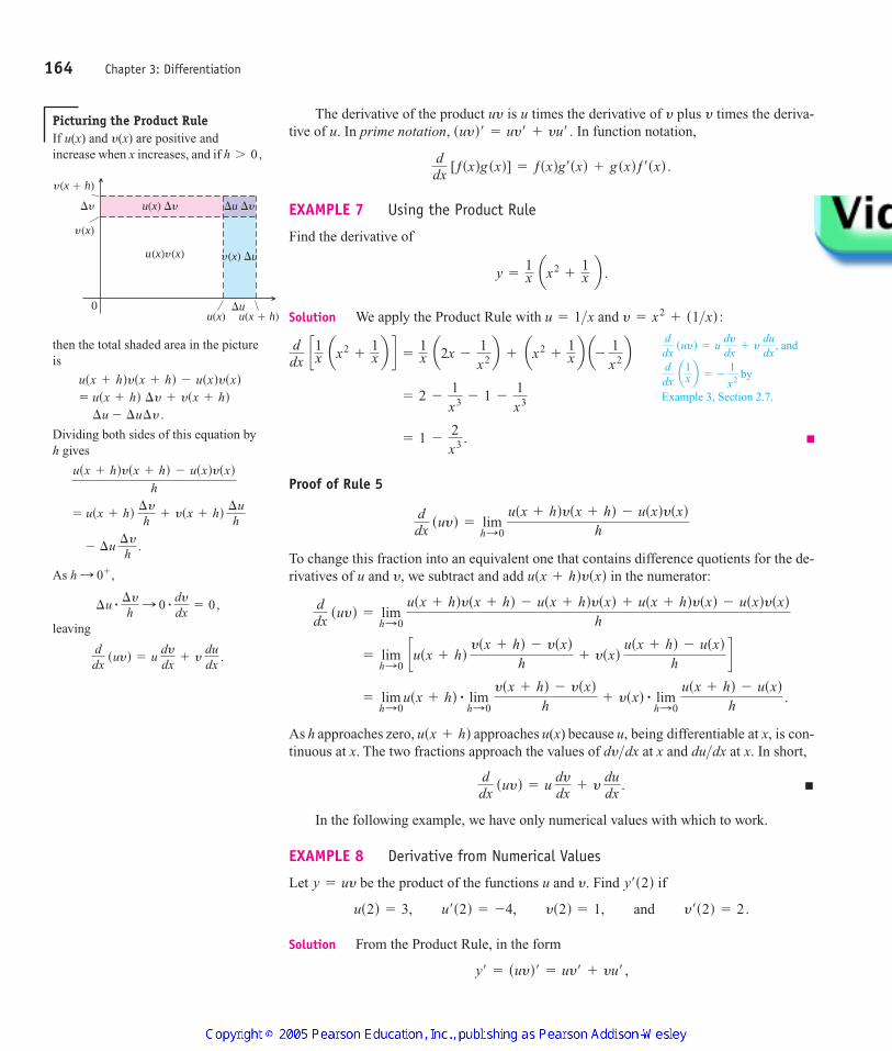
Picturing the Product RuleIf u(x) and y(x) are positive andincrease when x increases, and if h 7 0,

0

y(x � h)

y(x)

�y

u(x)y(x)

u(x) �y �u �y

y(x) �u

u(x � h)u(x)�u

then the total shaded area in the pictureis

Dividing both sides of this equation byh gives

As

leaving

ddx

suyd = u dydx

+ y dudx

.

¢u # ¢y

h: 0 # dy

dx= 0,

h : 0+ ,

- ¢u ¢y

h.

= usx + hd ¢y

h+ ysx + hd

¢uh

usx + hdysx + hd - usxdysxdh

¢u - ¢u¢y .= usx + hd ¢y + ysx + hdusx + hdysx + hd - usxdysxd



bounce03.htm*��g�<u

we have

EXAMPLE 9 Differentiating a Product in Two Ways


Solution

(a) From the Product Rule with and we find

(b) This particular product can be differentiated as well (perhaps better) by multiplyingout the original expression for y and differentiating the resulting polynomial:

This is in agreement with our first calculation.

Just as the derivative of the product of two differentiable functions is not the product oftheir derivatives, the derivative of the quotient of two functions is not the quotient of theirderivatives. What happens instead is the Quotient Rule.

dydx

= 5x4+ 3x2

+ 6x .

y = sx2+ 1dsx3

+ 3d = x5+ x3

+ 3x2+ 3

= 5x4+ 3x2

+ 6x .

= 3x4+ 3x2

+ 2x4+ 6x

ddx

C Ax2+ 1 B Ax3

+ 3 B D = sx2+ 1ds3x2d + sx3

+ 3ds2xd

y = x3+ 3,u = x2

+ 1

y = sx2+ 1dsx3

+ 3d .

= s3ds2d + s1ds -4d = 6 - 4 = 2.

y¿s2d = us2dy¿s2d + ys2du¿s2d


RULE 6 Derivative Quotient RuleIf u and y are differentiable at x and if then the quotient is differ-entiable at x, and

ddx

auy b =

y dudx

- u dydx

y2 .

u>yysxd Z 0,

In function notation,

EXAMPLE 10 Using the Quotient Rule


y =

t2- 1

t2+ 1

.

ddx

c ƒsxdg sxd

d =

g sxdƒ¿sxd - ƒsxdg¿sxdg2sxd

.



bounce03.html?1_5_l


SolutionWe apply the Quotient Rule with and

Proof of Rule 6

To change the last fraction into an equivalent one that contains the difference quotients forthe derivatives of u and y, we subtract and add y(x)u(x) in the numerator. We then get

Taking the limit in the numerator and denominator now gives the Quotient Rule.

Negative Integer Powers of x

The Power Rule for negative integers is the same as the rule for positive integers.

= limh:0

ysxd

usx + hd - usxdh

- usxd ysx + hd - ysxd

hysx + hdysxd

.

ddx

auy b = limh:0

ysxdusx + hd - ysxdusxd + ysxdusxd - usxdysx + hd

hysx + hdysxd

= limh:0

ysxdusx + hd - usxdysx + hd

hysx + hdysxd

ddx

auy b = limh:0

usx + hdysx + hd

-

usxdysxd

h

=

4tst2

+ 1d2 .

=

2t3+ 2t - 2t3

+ 2tst2

+ 1d2

ddt

auy b =

ysdu>dtd - usdy>dtd

y2 dydt

=

st2+ 1d # 2t - st2

- 1d # 2t

st2+ 1d2

y = t2+ 1:u = t2

- 1


RULE 7 Power Rule for Negative IntegersIf n is a negative integer and then

ddx

sxnd = nxn - 1 .

x Z 0,

EXAMPLE 11

(a) Agrees with Example 3, Section 2.7

(b)ddx

a 4x3 b = 4

ddx

sx-3d = 4s -3dx-4= -

12x4

ddx

a1x b =

ddx

sx-1d = s -1dx-2= -

1x2



Proof of Rule 7 The proof uses the Quotient Rule. If n is a negative integer, thenwhere m is a positive integer. Hence, and

Quotient Rule with and

Since

Since

EXAMPLE 12 Tangent to a Curve

Find an equation for the tangent to the curve

at the point (1, 3) (Figure 3.11).

Solution The slope of the curve is

The slope at is

The line through (1, 3) with slope is

Point-slope equation

The choice of which rules to use in solving a differentiation problem can make a dif-ference in how much work you have to do. Here is an example.

EXAMPLE 13 Choosing Which Rule to Use

Rather than using the Quotient Rule to find the derivative of

expand the numerator and divide by

y =

sx - 1dsx2- 2xd

x4 =

x3- 3x2

+ 2xx4 = x-1

- 3x-2+ 2x-3 .

x4 :

y =

sx - 1dsx2- 2xd

x4 ,

y = -x + 4.

y = -x + 1 + 3

y - 3 = s -1dsx - 1d

m = -1

dydx`x = 1

= c1 -2x2 d

x = 1= 1 - 2 = -1.

x = 1

dydx

=

ddx

sxd + 2 ddx

a1x b = 1 + 2 a- 1x2 b = 1 -

2x2 .

y = x +2x

-m = n = nxn - 1 .

= -mx-m - 1

m 7 0, ddx

sxmd = mxm - 1 =

0 - mxm - 1

x2m

y = xmu = 1 =

xm # ddx

A1 B - 1 # ddx

Axm Bsxmd2

ddx

sxnd =

ddx

a 1xm b

xn= x-m

= 1>xm ,n = -m ,


x

y

0

1

1 2

2

3

3

4

(1, 3)

y � –x � 4

y � x � 2x

FIGURE 3.11 The tangent to the curveat (1, 3) in Example 12.

The curve has a third-quadrant portionnot shown here. We see how to graphfunctions like this one in Chapter 4.

y = x + s2>xd



bounce03.html?1_6_l

bounce03.html?4_9_a


Then use the Sum and Power Rules:

Second- and Higher-Order Derivatives

If is a differentiable function, then its derivative is also a function. If isalso differentiable, then we can differentiate to get a new function of x denoted by So The function is called the second derivative of ƒ because it is the deriv-ative of the first derivative. Notationally,

The symbol means the operation of differentiation is performed twice.If then and we have

Thus

If is differentiable, its derivative, is the third derivativeof y with respect to x. The names continue as you imagine, with

denoting the nth derivative of y with respect to x for any positive integer n.We can interpret the second derivative as the rate of change of the slope of the tangent

to the graph of at each point. You will see in the next chapter that the second de-rivative reveals whether the graph bends upward or downward from the tangent line as wemove off the point of tangency. In the next section, we interpret both the second and thirdderivatives in terms of motion along a straight line.

EXAMPLE 14 Finding Higher Derivatives

The first four derivatives of are

First derivative:

Second derivative:

Third derivative:

Fourth derivative:

The function has derivatives of all orders, the fifth and later derivatives all being zero.

y s4d= 0.

y‡ = 6

y– = 6x - 6

y¿ = 3x2- 6x

y = x3- 3x2

+ 2

y = ƒsxd

y snd=

ddx

y sn - 1d=

dny

dxn = Dny

y‡ = dy–>dx = d3y>dx3y–

D2 Ax6 B = 30x4 .

y– =

dy¿

dx=

ddx

A6x5 B = 30x4 .

y¿ = 6x5y = x6 ,D2

ƒ–sxd =

d2y

dx2 =

ddx

adydxb =

dy¿

dx= y– = D2sƒdsxd = Dx

2 ƒsxd .

ƒ–ƒ– = sƒ¿d¿ .ƒ– .ƒ¿

ƒ¿ƒ¿sxdy = ƒsxd

= -1x2 +

6x3 -

6x4 .

dydx

= -x-2- 3s -2dx-3

+ 2s -3dx-4


How to Read the Symbols forDerivatives

“y prime”“y double prime”

“d squared y dx squared”

“y triple prime”“y super n”

“d to the n of y by dx to the n”

“D to the n”Dn

dny

dxn

y sndy‡

d2y

dx2

y–

y¿



bounce03.html?1_7_l





EXERCISES 3.2

Derivative CalculationsIn Exercises 1–12, find the first and second derivatives.

1. 2.

3. 4.

5. 6.

7. 8.

9. 10.

11. 12.

In Exercises 13–16, find (a) by applying the Product Rule and(b) by multiplying the factors to produce a sum of simpler terms todifferentiate.

13. 14.

15. 16.

Find the derivatives of the functions in Exercises 17–28.

17. 18.

19. 20.

21. 22.

23. 24.

25. 26.

27. 28.

Find the derivatives of all orders of the functions in Exercises 29 and30.

29. 30.

Find the first and second derivatives of the functions in Exercises31–38.

31. 32.

33. 34.

35. 36. w = sz + 1dsz - 1dsz2+ 1dw = a1 + 3z

3zb s3 - zd

u =

sx2+ xdsx2

- x + 1dx4r =

su - 1dsu2+ u + 1du3

s =

t2+ 5t - 1

t2y =

x3+ 7x

y =

x5

120y =

x4

2-

32

x2- x

y =

sx + 1dsx + 2dsx - 1dsx - 2d

y =

1sx2

- 1dsx2+ x + 1d

r = 2 a 12u + 2uby =

1 + x - 41xx

u =

5x + 121x

ƒssd =

1s - 11s + 1

w = s2x - 7d-1sx + 5dy = s1 - tds1 + t2d-1

ƒstd =

t2- 1

t2+ t - 2

g sxd =

x2- 4

x + 0.5

z =

2x + 1x2

- 1y =

2x + 53x - 2

y = ax +

1x b ax -

1x + 1by = sx2

+ 1d ax + 5 +

1x b

y = sx - 1dsx2+ x + 1dy = s3 - x2dsx3

- x + 1d

y¿

r =

12u

-

4u3 +

1u4r =

13s2 -

52s

y = 4 - 2x - x-3y = 6x2- 10x - 5x-2

s = -2t -1+

4t2w = 3z-2

-

1z

y =

x3

3+

x2

2+

x4

y =

4x3

3- x

w = 3z7- 7z3

+ 21z2s = 5t3- 3t5

y = x2+ x + 8y = -x2

+ 3

37. 38.

Using Numerical Values39. Suppose u and y are functions of x that are differentiable at

and that

Find the values of the following derivatives at

a. b. c. d.

40. Suppose u and y are differentiable functions of x and that

Find the values of the following derivatives at

a. b. c. d.

Slopes and Tangents41. a. Normal to a curve Find an equation for the line perpendicular

to the tangent to the curve at the point (2, 1).

b. Smallest slope What is the smallest slope on the curve? Atwhat point on the curve does the curve have this slope?

c. Tangents having specified slope Find equations for thetangents to the curve at the points where the slope of thecurve is 8.

42. a. Horizontal tangents Find equations for the horizontal tan-gents to the curve Also find equations forthe lines that are perpendicular to these tangents at the pointsof tangency.

b. Smallest slope What is the smallest slope on the curve? Atwhat point on the curve does the curve have this slope? Findan equation for the line that is perpendicular to the curve’stangent at this point.

43. Find the tangents to Newton’s serpentine (graphed here) at the ori-gin and the point (1, 2).

x

y

0

1

1 2

2(1, 2)

3 4

y � 4xx2 � 1

y = x3- 3x - 2.

y = x3- 4x + 1

ddx

s7y - 2udddx

ayu bddx

auy bddx

suyd

x = 1.

us1d = 2, u¿s1d = 0, ys1d = 5, y¿s1d = -1.

ddx

s7y - 2udddx

ayu bddx

auy bddx

suyd

x = 0.

us0d = 5, u¿s0d = -3, ys0d = -1, y¿s0d = 2.

x = 0

p =

q2+ 3

sq - 1d3+ sq + 1d3p = aq2

+ 3

12qb aq4

- 1

q3 b



tcu0302a.html

tcu0302a.html

tcu0302b.html

tcu0302b.html

tcu0302c.html

tcu0302c.html

tcu0302d.html

tcu0302d.html

tcu0302e.html

tcu0302e.html

tcu0302e.html

tcu0302e.html

tcu0302f.html

tcu0302f.html

tcu0302g.html

tcu0302g.html

44. Find the tangent to the Witch of Agnesi (graphed here) at the point(2, 1).

45. Quadratic tangent to identity function The curve passes through the point (1, 2) and is tangent to the

line at the origin. Find a, b, and c.

46. Quadratics having a common tangent The curves and have a common tangent line at

the point (1, 0). Find a, b, and c.

47. a. Find an equation for the line that is tangent to the curveat the point

b. Graph the curve and tangent line together. The tangentintersects the curve at another point. Use Zoom and Trace toestimate the point’s coordinates.

c. Confirm your estimates of the coordinates of the secondintersection point by solving the equations for the curve andtangent simultaneously (Solver key).

48. a. Find an equation for the line that is tangent to the curveat the origin.

b. Graph the curve and tangent together. The tangent intersectsthe curve at another point. Use Zoom and Trace to estimatethe point’s coordinates.

c. Confirm your estimates of the coordinates of the secondintersection point by solving the equations for the curve andtangent simultaneously (Solver key).

Theory and Examples49. The general polynomial of degree n has the form

where Find

50. The body’s reaction to medicine The reaction of the body to adose of medicine can sometimes be represented by an equation ofthe form

where C is a positive constant and M is the amount of medicineabsorbed in the blood. If the reaction is a change in blood pres-sure, R is measured in millimeters of mercury. If the reaction is achange in temperature, R is measured in degrees, and so on.

Find . This derivative, as a function of M, is called thesensitivity of the body to the medicine. In Section 4.5, we will see

dR>dM

R = M2 aC2

-

M3b ,

P¿sxd .an Z 0.

Psxd = an xn+ an - 1 xn - 1

+Á

+ a2 x2+ a1 x + a0

y = x3- 6x2

+ 5x

s -1, 0d .y = x3- x

y = cx - x2x2+ ax + b

y =

y = xax2

+ bx + cy =

x

y

0

1

1 2

2(2, 1)

3

y � 8x2 � 4

how to find the amount of medicine to which the body is mostsensitive.

51. Suppose that the function y in the Product Rule has a constantvalue c. What does the Product Rule then say? What does this sayabout the Constant Multiple Rule?

52. The Reciprocal Rule

a. The Reciprocal Rule says that at any point where the functiony(x) is differentiable and different from zero,

Show that the Reciprocal Rule is a special case of theQuotient Rule.

b. Show that the Reciprocal Rule and the Product Rule togetherimply the Quotient Rule.

53. Generalizing the Product Rule The Product Rule gives theformula

for the derivative of the product uy of two differentiable functionsof x.

a. What is the analogous formula for the derivative of theproduct uyw of three differentiable functions of x?

b. What is the formula for the derivative of the product of four differentiable functions of x?

c. What is the formula for the derivative of a productof a finite number n of differentiable functions

of x?

54. Rational Powers

a. Find by writing as and using the Product

Rule. Express your answer as a rational number times arational power of x. Work parts (b) and (c) by a similarmethod.

b. Find

c. Find

d. What patterns do you see in your answers to parts (a), (b), and(c)? Rational powers are one of the topics in Section 3.6.

55. Cylinder pressure If gas in a cylinder is maintained at a con-stant temperature T, the pressure P is related to the volume V by aformula of the form

in which a, b, n, and R are constants. Find . (See accompa-nying figure.)

dP>dV

P =

nRTV - nb

-

an2

V 2 ,

ddx

sx7>2d .

ddx

sx5>2d .

x # x1>2x3>2ddx

Ax3>2 B

u1 u2 u3 Á un

u1 u2 u3 u4

ddx

suyd = u dydx

+ y dudx

ddx

a1y b = -

1y2

dydx

.


T

T

T

T



tcu0302g.html

tcu0302g.html

56. The best quantity to order One of the formulas for inventorymanagement says that the average weekly cost of ordering, payingfor, and holding merchandise is

where q is the quantity you order when things run low (shoes, ra-dios, brooms, or whatever the item might be); k is the cost of plac-ing an order (the same, no matter how often you order); c is thecost of one item (a constant); m is the number of items sold eachweek (a constant); and h is the weekly holding cost per item (aconstant that takes into account things such as space, utilities, in-surance, and security). Find and d2A>dq2 .dA>dq

Asqd =

kmq + cm +

hq

2,

171


3.2 Differentiation Rules


3.4 Derivatives of Trigonometric Functions 183

Derivatives of Trigonometric Functions

Many of the phenomena we want information about are approximately periodic (electro-magnetic fields, heart rhythms, tides, weather). The derivatives of sines and cosines play akey role in describing periodic changes. This section shows how to differentiate the six ba-sic trigonometric functions.

Derivative of the Sine Function

To calculate the derivative of for x measured in radians, we combine the lim-its in Example 5a and Theorem 7 in Section 2.4 with the angle sum identity for the sine:

sin sx + hd = sin x cos h + cos x sin h .

ƒsxd = sin x ,

3.4



bounce03.html?5_2_a

If then

Derivative definition

Sine angle sum identity

= cos x . = sin x # 0 + cos x # 1

= sin x # limh:0

cos h - 1

h+ cos x # lim

h:0 sin h

h

= limh:0

asin x # cos h - 1h

b + limh:0

acos x # sin hhb

= limh:0

sin x scos h - 1d + cos x sin h

h

= limh:0

ssin x cos h + cos x sin hd - sin x

h

= limh:0

sin sx + hd - sin x

h

ƒ¿sxd = limh:0

ƒsx + hd - ƒsxd

h

ƒsxd = sin x ,


Example 5(a) andTheorem 7, Section 2.4

The derivative of the sine function is the cosine function:

ddx

ssin xd = cos x .

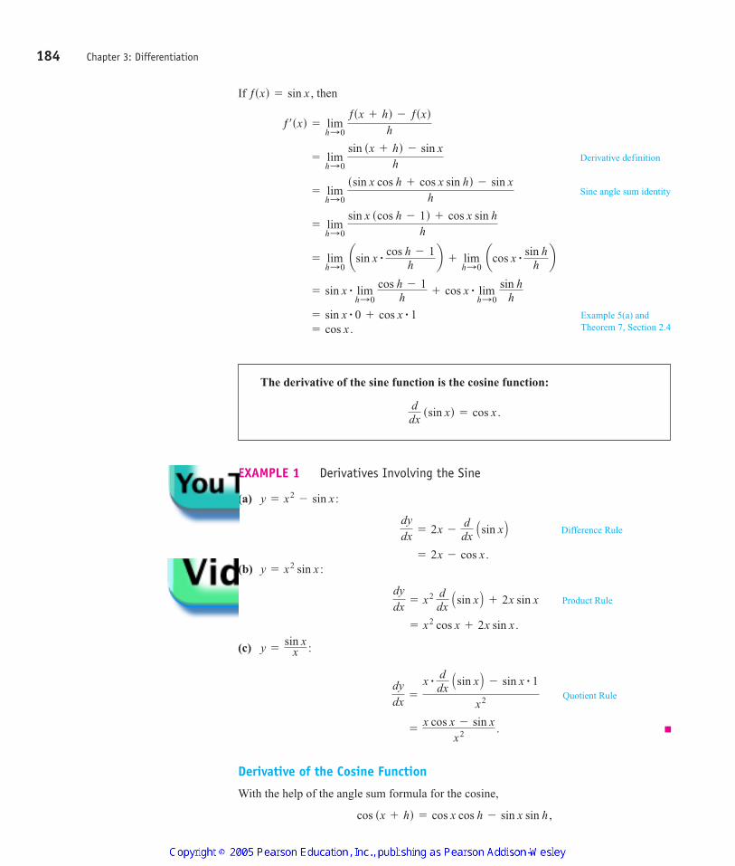
EXAMPLE 1 Derivatives Involving the Sine

(a)

Difference Rule

(b)

Product Rule

(c)

Quotient Rule

Derivative of the Cosine Function

With the help of the angle sum formula for the cosine,

cos sx + hd = cos x cos h - sin x sin h ,

=

x cos x - sin xx2 .

dydx

=

x # ddx

Asin x B - sin x # 1

x2

y =

sin xx :

= x2 cos x + 2x sin x .

dydx

= x2 ddx

Asin x B + 2x sin x

y = x2 sin x : = 2x - cos x .

dydx

= 2x -

ddx

Asin x By = x2

- sin x :



bounce03.html?2_4_l


we have

Derivative definition

= -sin x .

= cos x # 0 - sin x # 1

= cos x # limh:0

cos h - 1

h- sin x # lim

h:0 sin h

h

= limh:0

cos x # cos h - 1h

- limh:0

sin x # sin hh

= limh:0

cos xscos h - 1d - sin x sin h

h

= limh:0

scos x cos h - sin x sin hd - cos x

h

ddx

scos xd = limh:0

cos sx + hd - cos x

h


Cosine angle sumidentity

Example 5(a) andTheorem 7, Section 2.4

The derivative of the cosine function is the negative of the sine function:

ddx

scos xd = -sin x

1

x

y

0– –1

1

x

y'

0– –1

y � cos x

y' � –sin x

FIGURE 3.23 The curve asthe graph of the slopes of the tangents tothe curve y = cos x .

y¿ = -sin x

Figure 3.23 shows a way to visualize this result.

EXAMPLE 2 Derivatives Involving the Cosine

(a)

Sum Rule

(b)

Product Rule

(c)

Quotient Rule

=1

1 - sin x.

sin2 x + cos2 x = 1 =

1 - sin xs1 - sin xd2

=

s1 - sin xds -sin xd - cos xs0 - cos xds1 - sin xd2

dydx

=

A1 - sin x B ddx

Acos x B - cos x ddx

A1 - sin x Bs1 - sin xd2

y =

cos x1 - sin x

:

= cos2 x - sin2 x .

= sin xs -sin xd + cos xscos xd

dydx

= sin x ddx

Acos x B + cos x ddx

Asin x By = sin x cos x :

= 5 - sin x.

dydx

=

ddx

s5xd +

ddx

Acos x By = 5x + cos x :



bounce03.html?2_3_l



Simple Harmonic Motion

The motion of a body bobbing freely up and down on the end of a spring or bungee cord isan example of simple harmonic motion. The next example describes a case in which thereare no opposing forces such as friction or buoyancy to slow the motion down.

EXAMPLE 3 Motion on a Spring

A body hanging from a spring (Figure 3.24) is stretched 5 units beyond its rest positionand released at time to bob up and down. Its position at any later time t is

What are its velocity and acceleration at time t ?

Solution We have

Position:

Velocity:

Acceleration:

Notice how much we can learn from these equations:

1. As time passes, the weight moves down and up between and on thes-axis. The amplitude of the motion is 5. The period of the motion is

2. The velocity attains its greatest magnitude, 5, when as the graphsshow in Figure 3.25. Hence, the speed of the weight, is greatest when

that is, when (the rest position). The speed of the weight is zero whenThisoccurswhen at the endpoints of the interval of motion.

3. The acceleration value is always the exact opposite of the position value. When theweight is above the rest position, gravity is pulling it back down; when the weight isbelow the rest position, the spring is pulling it back up.

4. The acceleration, is zero only at the rest position, where andthe force of gravity and the force from the spring offset each other. When the weight isanywhere else, the two forces are unequal and acceleration is nonzero. The accelera-tion is greatest in magnitude at the points farthest from the rest position, where

EXAMPLE 4 Jerk

The jerk of the simple harmonic motion in Example 3 is

It has its greatest magnitude when not at the extremes of the displacement butat the rest position, where the acceleration changes direction and sign.

Derivatives of the Other Basic Trigonometric Functions

Because sin x and cos x are differentiable functions of x, the related functions

tan x =

sin xcos x , cot x =

cos xsin x

, sec x =1

cos x , and csc x =1

sin x

sin t = ;1,

j =

dadt

=

ddt

s -5 cos td = 5 sin t .

cos t = ;1.

cos t = 0a = -5 cos t ,

s = 5 cos t = ;5,sin t = 0.s = 0cos t = 0,

ƒ y ƒ = 5 ƒ sin t ƒ ,cos t = 0,y = -5 sin t

2p .s = 5s = -5

a =

dydt

=

ddt

s -5 sin td = -5 cos t .

y =

dsdt

=

ddt

s5 cos td = -5 sin t

s = 5 cos t

s = 5 cos t .

t = 0


s

0

–5

5

Restposition

Position att � 0

FIGURE 3.24 A body hanging froma vertical spring and then displacedoscillates above and below its rest position.Its motion is described by trigonometricfunctions (Example 3).

t0

s, y

y � –5 sin t s � 5 cos t

� �2

3� 2�2

5�2

FIGURE 3.25 The graphs of the positionand velocity of the body in Example 3.



bounce03.html?2_7_l

are differentiable at every value of x at which they are defined. Their derivatives, calcu-lated from the Quotient Rule, are given by the following formulas. Notice the negativesigns in the derivative formulas for the cofunctions.


Derivatives of the Other Trigonometric Functions

ddx

scsc xd = -csc x cot x

ddx

scot xd = -csc2 x

ddx

ssec xd = sec x tan x

ddx

stan xd = sec2 x

To show a typical calculation, we derive the derivative of the tangent function. Theother derivations are left to Exercise 50.

EXAMPLE 5

Find d(tan x) dx.

Solution

Quotient Rule

EXAMPLE 6

Find

Solution

Product Rule

= sec3 x + sec x tan2 x

= sec xssec2 xd + tan xssec x tan xd

= sec x ddx

A tan x B + tan x ddx

Asec x B y– =

ddx

ssec x tan xd

y¿ = sec x tan x

y = sec x

y– if y = sec x .

=1

cos2 x= sec2 x

=

cos2 x + sin2 xcos2 x

=

cos x cos x - sin x s -sin xdcos2 x

ddx

A tan x B =

ddx

a sin xcos x b =

cos x ddx

Asin x B - sin x ddx

Acos x Bcos2 x

>

4100 AWL/Thomas_ch03p147-243 8/19/04 11:16 AM 7


bounce03.html?2_5_l


The differentiability of the trigonometric functions throughout their domains givesanother proof of their continuity at every point in their domains (Theorem 1, Section 3.1).So we can calculate limits of algebraic combinations and composites of trigonometricfunctions by direct substitution.

EXAMPLE 7 Finding a Trigonometric Limit

limx:0

22 + sec x

cos sp - tan xd=

22 + sec 0cos sp - tan 0d

=

22 + 1cos sp - 0d

=

23-1

= -23




bounce03.html?2_6_l


EXERCISES 3.4

DerivativesIn Exercises 1–12, find .

1. 2.

3. 4.

5.

6.

7. 8.

9. 10.

11.

12.

In Exercises 13–16, find .

13. 14.

15. 16.

In Exercises 17–20, find

17. 18.

19. 20.

In Exercises 21–24, find .

21. 22.

23. 24.

25. Find if

a. b. y = sec x .y = csc x .

y–

p =

tan q

1 + tan qp =

sin q + cos qcos q

p = s1 + csc qd cos qp = 5 +

1cot q

dp>dq

r = s1 + sec ud sin ur = sec u csc u

r = u sin u + cos ur = 4 - u2 sin u

dr>du .

s =

sin t1 - cos t

s =

1 + csc t1 - csc t

s = t2- sec t + 1s = tan t - t

ds>dt

y = x2 cos x - 2x sin x - 2 cos x

y = x2 sin x + 2x cos x - 2 sin x

y =

cos xx +

xcos xy =

4cos x +

1tan x

y =

cos x1 + sin x

y =

cot x1 + cot x

y = ssin x + cos xd sec x

y = ssec x + tan xdssec x - tan xd

y = x2 cot x -

1x2y = csc x - 41x + 7

y =

3x + 5 sin xy = -10x + 3 cos x

dy>dx

26. Find if

a. b.

Tangent LinesIn Exercises 27–30, graph the curves over the given intervals, togetherwith their tangents at the given values of x. Label each curve and tan-gent with its equation.

27.

28.

29.

30.

Do the graphs of the functions in Exercises 31–34 have any horizontaltangents in the interval If so, where? If not, why not?Visualize your findings by graphing the functions with a grapher.

31.

32.

33.

34.

35. Find all points on the curve wherethe tangent line is parallel to the line Sketch the curveand tangent(s) together, labeling each with its equation.

36. Find all points on the curve where thetangent line is parallel to the line Sketch the curve andtangent(s) together, labeling each with its equation.

y = -x .y = cot x, 0 6 x 6 p ,

y = 2x .y = tan x, -p>2 6 x 6 p>2,

y = x + 2 cos x

y = x - cot x

y = 2x + sin x

y = x + sin x

0 … x … 2p?

x = -p>3, 3p>2 y = 1 + cos x, -3p>2 … x … 2p

x = -p>3, p>4 y = sec x, -p>2 6 x 6 p>2 x = -p>3, 0, p>3 y = tan x, -p>2 6 x 6 p>2 x = -p, 0, 3p>2 y = sin x, -3p>2 … x … 2p

y = 9 cos x .y = -2 sin x .

y s4d= d4 y>dx4

T



tcu0304a.html

tcu0304a.html

tcu0304b.html

tcu0304b.html

tcu0304c.html

tcu0304c.html

tcu0304d.html

tcu0304d.html

tcu0304e.html

tcu0304e.html

In Exercises 37 and 38, find an equation for (a) the tangent to thecurve at P and (b) the horizontal tangent to the curve at Q.

37. 38.

Trigonometric LimitsFind the limits in Exercises 39–44.

39.

40.

41.

42.

43.

44.

Simple Harmonic MotionThe equations in Exercises 45 and 46 give the position of abody moving on a coordinate line (s in meters, t in seconds). Find thebody’s velocity, speed, acceleration, and jerk at time

45. 46.

Theory and Examples47. Is there a value of c that will make

continuous at Give reasons for your answer.x = 0?

ƒsxd = L sin2 3x

x2 , x Z 0

c, x = 0

s = sin t + cos ts = 2 - 2 sin t

t = p>4 sec .

s = ƒstd

limu:0

cos a pusin u

b

limt:0

tan a1 -

sin tt b

limx:0

sin a p + tan xtan x - 2 sec x

b

limx:0

sec ccos x + p tan a p

4 sec xb - 1 d

limx: -p>621 + cos sp csc xd

limx:2

sin a1x -

12b

x

y

0 1 2

4

3

Q

�4

P , 4

�4

y � 1 � �2 csc x � cot x

x

y

0

1

1 2

2

Q

y � 4 � cot x � 2csc x

�2

P , 2

�2

48. Is there a value of b that will make

continuous at Differentiable at Give reasons foryour answers.

49. Find

50. Derive the formula for the derivative with respect to x of

a. sec x. b. csc x. c. cot x.

51. Graph for On the same screen, graph

for and 0.1. Then, in a new window, tryand What happens as As

What phenomenon is being illustrated here?

52. Graph for On the same screen, graph

for and 0.1. Then, in a new window, tryand What happens as As

What phenomenon is being illustrated here?

53. Centered difference quotients The centered difference quotient

is used to approximate in numerical work because (1) itslimit as equals when exists, and (2) it usuallygives a better approximation of for a given value of h thanFermat’s difference quotient

See the accompanying figure.

ƒsx + hd - ƒsxdh

.

ƒ¿sxdƒ¿sxdƒ¿sxdh : 0

ƒ¿sxd

ƒsx + hd - ƒsx - hd2h

h : 0- ?h : 0+ ?-0.3 .h = -1, -0.5 ,

h = 1, 0.5, 0.3 ,

y =

cos sx + hd - cos x

h

-p … x … 2p .y = -sin x

h : 0- ?h : 0+ ?-0.3 .h = -1, -0.5 ,

h = 1, 0.5, 0.3 ,

y =

sin sx + hd - sin x

h

-p … x … 2p .y = cos x

d999>dx999 scos xd .

x = 0?x = 0?

g sxd = e x + b, x 6 0

cos x, x Ú 0


T

T

T

x

y

0 x

A

hh

C B

x � h x � h

y � f (x)

Slope � f '(x)

Slope �

Slope �

hf (x � h) � f (x)

f (x � h) � f (x � h)2h



tcu0304f.html

tcu0304f.html

tcu0304g.html

tcu0304g.html

tcu0304h.html

tcu0304h.html

a. To see how rapidly the centered difference quotient forconverges to graph

together with

over the interval for and 0.3. Comparethe results with those obtained in Exercise 51 for the samevalues of h.

b. To see how rapidly the centered difference quotient forconverges to graph

together with

over the interval and 0.3. Comparethe results with those obtained in Exercise 52 for the samevalues of h.

54. A caution about centered difference quotients (Continuationof Exercise 53.) The quotient

may have a limit as when ƒ has no derivative at x. As a casein point, take and calculate

As you will see, the limit exists even though has no de-rivative at Moral: Before using a centered difference quo-tient, be sure the derivative exists.

55. Slopes on the graph of the tangent function Graph and its derivative together on Does the graph of thetangent function appear to have a smallest slope? a largest slope?Is the slope ever negative? Give reasons for your answers.

s -p>2, p>2d .y = tan x

x = 0.ƒsxd = ƒ x ƒ

limh:0

ƒ 0 + h ƒ - ƒ 0 - h ƒ

2h.

ƒsxd = ƒ x ƒ

h : 0

ƒsx + hd - ƒsx - hd2h

[-p, 2p] for h = 1, 0.5 ,

y =

cos sx + hd - cos sx - hd2h

y = -sin xƒ¿sxd = -sin x ,ƒsxd = cos x

h = 1, 0.5 ,[-p, 2p]

y =

sin sx + hd - sin sx - hd2h

y = cos xƒ¿sxd = cos x ,ƒsxd = sin x56. Slopes on the graph of the cotangent function Graph

and its derivative together for Does thegraph of the cotangent function appear to have a smallest slope?A largest slope? Is the slope ever positive? Give reasons for youranswers.

57. Exploring (sin kx) x Graph andtogether over the interval Where

does each graph appear to cross the y-axis? Do the graphs reallyintersect the axis? What would you expect the graphs of

and to do as Why?What about the graph of for other values of k?Give reasons for your answers.

58. Radians versus degrees: degree mode derivatives What hap-pens to the derivatives of sin x and cos x if x is measured in de-grees instead of radians? To find out, take the following steps.

a. With your graphing calculator or computer grapher in degreemode, graph

and estimate Compare your estimate withIs there any reason to believe the limit should be

b. With your grapher still in degree mode, estimate

c. Now go back to the derivation of the formula for thederivative of sin x in the text and carry out the steps of thederivation using degree-mode limits. What formula do youobtain for the derivative?

d. Work through the derivation of the formula for the derivativeof cos x using degree-mode limits. What formula do youobtain for the derivative?

e. The disadvantages of the degree-mode formulas becomeapparent as you start taking derivatives of higher order. Try it.What are the second and third degree-mode derivatives ofsin x and cos x?

limh:0

cos h - 1

h.

p>180?p>180.limh:0 ƒshd .

ƒshd =

sin hh

y = ssin kxd>xx : 0?y = ssin s -3xdd>xy = ssin 5xd>x

-2 … x … 2.y = ssin 4xd>xy = ssin 2xd>x ,y = ssin xd>x ,/

0 6 x 6 p .y = cot x


T

T

T

T



OVERVIEW This chapter studies some of the important applications of derivatives. Welearn how derivatives are used to find extreme values of functions, to determine and ana-lyze the shapes of graphs, to calculate limits of fractions whose numerators and denomina-tors both approach zero or infinity, and to find numerically where a function equals zero.We also consider the process of recovering a function from its derivative. The key to manyof these accomplishments is the Mean Value Theorem, a theorem whose corollaries pro-vide the gateway to integral calculus in Chapter 5.

244

APPLICATIONS OF

DERIVATIVES

C h a p t e r

4

Extreme Values of Functions

This section shows how to locate and identify extreme values of a continuous functionfrom its derivative. Once we can do this, we can solve a variety of optimization problemsin which we find the optimal (best) way to do something in a given situation.

4.1

DEFINITIONS Absolute Maximum, Absolute MinimumLet ƒ be a function with domain D. Then ƒ has an absolute maximum value onD at a point c if

and an absolute minimum value on D at c if

ƒsxd Ú ƒscd for all x in D .

ƒsxd … ƒscd for all x in D

Absolute maximum and minimum values are called absolute extrema (plural of the Latinextremum). Absolute extrema are also called global extrema, to distinguish them fromlocal extrema defined below.

For example, on the closed interval the function takes onan absolute maximum value of 1 (once) and an absolute minimum value of 0 (twice). Onthe same interval, the function takes on a maximum value of 1 and a mini-mum value of (Figure 4.1).

Functions with the same defining rule can have different extrema, depending on thedomain.

-1g sxd = sin x

ƒsxd = cos x[-p>2, p>2]

x

y

0

1y � sin x

y � cos x

–1

�2

–�2

FIGURE 4.1 Absolute extrema forthe sine and cosine functions on

These values can dependon the domain of a function.[-p>2, p>2] .



bounce04.html?3_7_a

4.1 Extreme Values of Functions 245

EXAMPLE 1 Exploring Absolute Extrema

The absolute extrema of the following functions on their domains can be seen in Figure 4.2.

x2

(a) abs min only

y � x2

D � (–�, �)

y

x2

(b) abs max and min

y � x2

D � [0, 2]

y

x2

(d) no max or min

y � x2

D � (0, 2)

y

x2

(c) abs max only

y � x2

D � (0, 2]

y

FIGURE 4.2 Graphs for Example 1.

Function rule Domain D Absolute extrema on D

(a) No absolute maximum.Absolute minimum of 0 at

(b) [0, 2] Absolute maximum of 4 at Absolute minimum of 0 at

(c) (0, 2] Absolute maximum of 4 at No absolute minimum.

(d) (0, 2) No absolute extrema.y = x2

x = 2.y = x2

x = 0.x = 2.y = x2

x = 0.s - q , q dy = x2

HISTORICAL BIOGRAPHY

Daniel Bernoulli(1700–1789)

The following theorem asserts that a function which is continuous at every point of aclosed interval [a, b] has an absolute maximum and an absolute minimum value on the in-terval. We always look for these values when we graph a function.

4100 AWL/Thomas_ch04p244-324 8/20/04 9:01 AM 5


The proof of The Extreme Value Theorem requires a detailed knowledge of the realnumber system (see Appendix 4) and we will not give it here. Figure 4.3 illustrates possi-ble locations for the absolute extrema of a continuous function on a closed interval [a, b].As we observed for the function it is possible that an absolute minimum (or ab-solute maximum) may occur at two or more different points of the interval.

The requirements in Theorem 1 that the interval be closed and finite, and that thefunction be continuous, are key ingredients. Without them, the conclusion of the theoremneed not hold. Example 1 shows that an absolute extreme value may not exist if the inter-val fails to be both closed and finite. Figure 4.4 shows that the continuity requirement can-not be omitted.

Local (Relative) Extreme Values

Figure 4.5 shows a graph with five points where a function has extreme values on its domain[a, b]. The function’s absolute minimum occurs at a even though at e the function’s value is

y = cos x ,

246 Chapter 4: Applications of Derivatives

xa x2

x2

Maximum and minimumat interior points

b

M

xa b

M

m

Maximum and minimumat endpoints

xa

Maximum at interior point,minimum at endpoint

M

b

mx

a

Minimum at interior point,maximum at endpoint

M

b

m

(x2, M)

(x1, m)

x1

y � f (x)

y � f (x)

y � f (x)

y � f (x)

x1

�m�

FIGURE 4.3 Some possibilities for a continuous function’s maximum andminimum on a closed interval [a, b].

THEOREM 1 The Extreme Value TheoremIf ƒ is continuous on a closed interval [a, b], then ƒ attains both an absolute max-imum value M and an absolute minimum value m in [a, b]. That is, there arenumbers and in [a, b] with and forevery other x in [a, b] (Figure 4.3).

m … ƒsxd … Mƒsx1d = m, ƒsx2d = M ,x2x1

x

y

1Smallest value

0

No largest value

1

y � x0 � x � 1

FIGURE 4.4 Even a single point ofdiscontinuity can keep a function fromhaving either a maximum or minimumvalue on a closed interval. The function

is continuous at every point of [0, 1]except yet its graph over [0, 1]does not have a highest point.

x = 1,

y = e x, 0 … x 6 1

0, x = 1



bounce04.html?1_0_l

bounce04.html?3_6_a


smaller than at any other point nearby. The curve rises to the left and falls to the rightaround c, making ƒ(c) a maximum locally. The function attains its absolute maximum at d.

xba c e d

Local minimumNo smaller value off nearby.

Local minimumNo smaller valueof f nearby.

Local maximumNo greater value of

f nearby.

Absolute minimumNo smaller value off anywhere. Also a

local minimum.

Absolute maximumNo greater value of f anywhere.Also a local maximum.

y � f (x)

FIGURE 4.5 How to classify maxima and minima.

DEFINITIONS Local Maximum, Local MinimumA function ƒ has a local maximum value at an interior point c of its domain if

A function ƒ has a local minimum value at an interior point c of its domain if

ƒsxd Ú ƒscd for all x in some open interval containing c .

ƒsxd … ƒscd for all x in some open interval containing c .

THEOREM 2 The First Derivative Theorem for Local Extreme ValuesIf ƒ has a local maximum or minimum value at an interior point c of its domain,and if is defined at c, then

ƒ¿scd = 0.

ƒ¿

We can extend the definitions of local extrema to the endpoints of intervals by defining ƒto have a local maximum or local minimum value at an endpoint c if the appropriate in-equality holds for all x in some half-open interval in its domain containing c. In Figure 4.5,the function ƒ has local maxima at c and d and local minima at a, e, and b. Local extremaare also called relative extrema.

An absolute maximum is also a local maximum. Being the largest value overall, it isalso the largest value in its immediate neighborhood. Hence, a list of all local maxima willautomatically include the absolute maximum if there is one. Similarly, a list of all localminima will include the absolute minimum if there is one.

Finding Extrema

The next theorem explains why we usually need to investigate only a few values to find afunction’s extrema.



Proof To prove that is zero at a local extremum, we show first that cannot bepositive and second that cannot be negative. The only number that is neither positivenor negative is zero, so that is what must be.

To begin, suppose that ƒ has a local maximum value at (Figure 4.6) so thatfor all values of x near enough to c. Since c is an interior point of ƒ’s do-

main, is defined by the two-sided limit

This means that the right-hand and left-hand limits both exist at and equal When we examine these limits separately, we find that

(1)

Similarly,

(2)

Together, Equations (1) and (2) imply This proves the theorem for local maximum values. To prove it for local mini-

mum values, we simply use which reverses the inequalities in Equations (1)and (2).

Theorem 2 says that a function’s first derivative is always zero at an interior pointwhere the function has a local extreme value and the derivative is defined. Hence the onlyplaces where a function ƒ can possibly have an extreme value (local or global) are

1. interior points where

2. interior points where is undefined,

3. endpoints of the domain of ƒ.

The following definition helps us to summarize.

ƒ¿

ƒ¿ = 0,

ƒsxd Ú ƒscd ,

ƒ¿scd = 0.

ƒ¿scd = limx:c-

ƒsxd - ƒscd

x - c Ú 0.

ƒ¿scd = limx:c+

ƒsxd - ƒscd

x - c … 0.

ƒ¿scd .x = c

limx:c

ƒsxd - ƒscd

x - c .

ƒ¿scdƒsxd - ƒscd … 0

x = cƒ¿scd

ƒ¿scdƒ¿scdƒ¿scd


Because and ƒsxd … ƒscd

sx - cd 7 0

Because and ƒsxd … ƒscd

sx - cd 6 0

xc x

Local maximum value

x

Secant slopes � 0(never negative)

Secant slopes � 0(never positive)

y � f (x)

FIGURE 4.6 A curve with a localmaximum value. The slope at c,simultaneously the limit of nonpositivenumbers and nonnegative numbers, is zero.

DEFINITION Critical PointAn interior point of the domain of a function ƒ where is zero or undefined is acritical point of ƒ.

ƒ¿

Thus the only domain points where a function can assume extreme values are criticalpoints and endpoints.

Be careful not to misinterpret Theorem 2 because its converse is false. A differen-tiable function may have a critical point at without having a local extreme valuethere. For instance, the function has a critical point at the origin and zero valuethere, but is positive to the right of the origin and negative to the left. So it cannot have alocal extreme value at the origin. Instead, it has a point of inflection there. This idea is de-fined and discussed further in Section 4.4.

Most quests for extreme values call for finding the absolute extrema of a continuousfunction on a closed and finite interval. Theorem 1 assures us that such values exist; Theo-rem 2 tells us that they are taken on only at critical points and endpoints. Often we can

ƒsxd = x3x = c




simply list these points and calculate the corresponding function values to find what thelargest and smallest values are, and where they are located.

How to Find the Absolute Extrema of a Continuous Function ƒ on aFinite Closed Interval1. Evaluate ƒ at all critical points and endpoints.

2. Take the largest and smallest of these values.

EXAMPLE 2 Finding Absolute Extrema

Find the absolute maximum and minimum values of on

Solution The function is differentiable over its entire domain, so the only critical point iswhere namely We need to check the function’s values at and at the endpoints and

Critical point value:

Endpoint values:

The function has an absolute maximum value of 4 at and an absolute minimumvalue of 0 at

EXAMPLE 3 Absolute Extrema at Endpoints

Find the absolute extrema values of on

Solution The function is differentiable on its entire domain, so the only critical pointsoccur where Solving this equation gives

a point not in the given domain. The function’s absolute extrema therefore occur at theendpoints, (absolute minimum), and (absolute maximum). SeeFigure 4.7.

EXAMPLE 4 Finding Absolute Extrema on a Closed Interval

Find the absolute maximum and minimum values of on the interval

Solution We evaluate the function at the critical points and endpoints and take thelargest and smallest of the resulting values.

The first derivative

has no zeros but is undefined at the interior point The values of ƒ at this one criti-cal point and at the endpoints are

Critical point value:

Endpoint values:

ƒs3d = s3d2>3= 23 9 .

ƒs -2d = s -2d2>3= 23 4

ƒs0d = 0

x = 0.

ƒ¿sxd =23

x-1>3=

2

323 x

[-2, 3] .ƒsxd = x2>3

g s1d = 7g s -2d = -32

8 - 4t3= 0 or t = 23 2 7 1,

g¿std = 0.

[-2, 1] .g std = 8t - t4

x = 0.x = -2

ƒs1d = 1

ƒs -2d = 4

ƒs0d = 0

x = 1:x = -2x = 0x = 0.ƒ¿sxd = 2x = 0,

[-2, 1] .ƒsxd = x2

(–2, –32)

(1, 7)

y � 8t � t4

–32

7

1–1–2t

y

FIGURE 4.7 The extreme values ofon (Example 3).[-2, 1]g std = 8t - t4



bounce04.html?1_1_l

bounce04.html?1_2_l


We can see from this list that the function’s absolute maximum value is and itoccurs at the right endpoint The absolute minimum value is 0, and it occurs at theinterior point (Figure 4.8).

While a function’s extrema can occur only at critical points and endpoints, not everycritical point or endpoint signals the presence of an extreme value. Figure 4.9 illustratesthis for interior points.

We complete this section with an example illustrating how the concepts we studiedare used to solve a real-world optimization problem.

EXAMPLE 5 Piping Oil from a Drilling Rig to a Refinery

A drilling rig 12 mi offshore is to be connected by pipe to a refinery onshore, 20 mistraight down the coast from the rig. If underwater pipe costs $500,000 per mile and land-based pipe costs $300,000 per mile, what combination of the two will give the least expen-sive connection?

Solution We try a few possibilities to get a feel for the problem:

(a) Smallest amount of underwater pipe

Underwater pipe is more expensive, so we use as little as we can. We run straight toshore (12 mi) and use land pipe for 20 mi to the refinery.

(b) All pipe underwater (most direct route)

We go straight to the refinery underwater.

This is less expensive than plan (a).

L 11,661,900

Dollar cost = 2544 s500,000d

20

12

Rig

Refinery

�144 + 400

= 12,000,000

Dollar cost = 12s500,000d + 20s300,000d

20

12

Rig

Refinery

x = 0.x = 3.

23 9 L 2.08,


x

y

10 2 3–1–2

1

2

Absolute maximum;also a local maximumLocal

maximum

Absolute minimum;also a local minimum

y � x2/3, –2 ≤ x ≤ 3

FIGURE 4.8 The extreme values ofon occur at and

(Example 4).x = 3x = 0[-2, 3]ƒsxd = x2>3

–1

x

y

1–1

1

0

(a)

y � x3

–1

x

y

1–1

1

0

(b)

y � x1/3

FIGURE 4.9 Critical points withoutextreme values. (a) is 0 at

but has no extremum there.(b) is undefined at but has no extremum there.y = x1>3

x = 0,y¿ = s1>3dx-2>3y = x3x = 0,

y¿ = 3x2



bounce04.html?1_3_l

bounce04.html?4_7



(c) Something in between

Now we introduce the length x of underwater pipe and the length y of land-based pipeas variables. The right angle opposite the rig is the key to expressing the relationship be-tween x and y, for the Pythagorean theorem gives

(3)

Only the positive root has meaning in this model.The dollar cost of the pipeline is

To express c as a function of a single variable, we can substitute for x, using Equation (3):

Our goal now is to find the minimum value of c(y) on the interval Thefirst derivative of c(y) with respect to y according to the Chain Rule is

Setting equal to zero gives

y = 11 or y = 29.

y = 20 ; 9

s20 - yd = ;

34

# 12 = ;9

169

A20 - y B2 = 144

259

A20 - y B2 = 144 + s20 - yd2

53

A20 - y B = 2144 + s20 - yd2

500,000 s20 - yd = 300,0002144 + s20 - yd2

c¿

= -500,000 20 - y2144 + s20 - yd2

+ 300,000.

c¿s yd = 500,000 # 12

#2s20 - yds -1d2144 + s20 - yd2

+ 300,000

0 … y … 20.

cs yd = 500,0002144 + s20 - yd2+ 300,000y .

c = 500,000x + 300,000y .

x = 2144 + s20 - yd2 .

x2= 122

+ s20 - yd2

12 mi

Rig

Refinery

20 – y y

20 mi

x




Only lies in the interval of interest. The values of c at this one critical point and atthe endpoints are

The least expensive connection costs $10,800,000, and we achieve it by running the lineunderwater to the point on shore 11 mi from the refinery.

cs20d = 12,000,000

cs0d = 11,661,900

cs11d = 10,800,000

y = 11




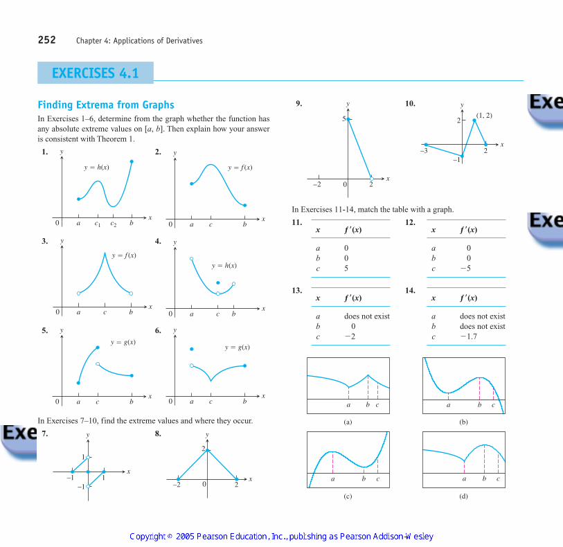
EXERCISES 4.1

Finding Extrema from GraphsIn Exercises 1–6, determine from the graph whether the function hasany absolute extreme values on [a, b]. Then explain how your answeris consistent with Theorem 1.

1. 2.

3. 4.

5. 6.

In Exercises 7–10, find the extreme values and where they occur.

7. 8.

2

2

–2 0

y

x1–1

1

–1

y

x

x

y

0 a c b

y � g(x)

x

y

0 a c b

y � g(x)

x

y

0 a bc

y � h(x)

x

y

0 a bc

y � f (x)

x

y

0 a c b

y � f (x)

x

y

0 a c1 bc2

y � h(x)

9. 10.

In Exercises 11-14, match the table with a graph.

11. 12.

13. 14.x ƒ �(x)

a does not existb does not existc �1.7

x ƒ �(x)

a does not existb 0c �2

x ƒ �(x)

a 0b 0c �5

x ƒ �(x)

a 0b 0c 5

2(1, 2)

–3 2–1

x

y

0 2–2

5

x

y

a b c a b c

a b c a b c

(a) (b)

(c) (d)



tcu0401a.html

tcu0401a.html

tcu0401a.html

tcu0401a.html

tcu0401b.html

tcu0401b.html


Absolute Extrema on Finite Closed IntervalsIn Exercises 15–30, find the absolute maximum and minimum valuesof each function on the given interval. Then graph the function. Iden-tify the points on the graph where the absolute extrema occur, and in-clude their coordinates.

15.

16.

17.

18.

19.

20.

21.

22.

23.

24.

25.

26.

27.

28.

29.

30.

In Exercises 31–34, find the function’s absolute maximum and mini-mum values and say where they are assumed.

31.

32.

33.

34.

Finding Extreme ValuesIn Exercises 35–44, find the extreme values of the function and wherethey occur.

35. 36.

37. 38.

39. 40.

41. 42.

43. 44. y =

x + 1x2

+ 2x + 2y =

x

x2+ 1

y = 23 + 2x - x2y =

123 1 - x2

y =

121 - x2y = 2x2

- 1

y = x3- 3x2

+ 3x - 2y = x3+ x2

- 8x + 5

y = x3- 2x + 4y = 2x2

- 8x + 9

hsud = 3u2>3, -27 … u … 8

g sud = u3>5, -32 … u … 1

ƒsxd = x5>3, -1 … x … 8

ƒsxd = x4>3, -1 … x … 8

ƒstd = ƒ t - 5 ƒ , 4 … t … 7

ƒstd = 2 - ƒ t ƒ , -1 … t … 3

g sxd = sec x, -

p

3… x …

p

6

g sxd = csc x, p3

… x …

2p3

ƒsud = tan u, -

p

3… u …

p

4

ƒsud = sin u, -

p

2… u …

5p6

g sxd = -25 - x2, -25 … x … 0

g sxd = 24 - x2, -2 … x … 1

hsxd = -3x2>3, -1 … x … 1

hsxd = 23 x, -1 … x … 8

Fsxd = -

1x , -2 … x … -1

Fsxd = -

1x2 , 0.5 … x … 2

ƒsxd = 4 - x2, -3 … x … 1

ƒsxd = x2- 1, -1 … x … 2

ƒsxd = -x - 4, -4 … x … 1

ƒsxd =

23

x - 5, -2 … x … 3

Local Extrema and Critical PointsIn Exercises 45–52, find the derivative at each critical point and deter-mine the local extreme values.

45. 46.

47. 48.

49. 50.

51.

52.

In Exercises 53 and 54, give reasons for your answers.

53. Let

a. Does exist?

b. Show that the only local extreme value of ƒ occurs at

c. Does the result in part (b) contradict the Extreme ValueTheorem?

d. Repeat parts (a) and (b) for replacing 2by a.

54. Let

a. Does exist?

b. Does exist?

c. Does exist?

d. Determine all extrema of ƒ.

Optimization ApplicationsWhenever you are maximizing or minimizing a function of a singlevariable, we urge you to graph the function over the domain that is ap-propriate to the problem you are solving. The graph will provide in-sight before you begin to calculate and will furnish a visual context forunderstanding your answer.

55. Constructing a pipeline Supertankers off-load oil at a dockingfacility 4 mi offshore. The nearest refinery is 9 mi east of theshore point nearest the docking facility. A pipeline must be con-structed connecting the docking facility with the refinery. Thepipeline costs $300,000 per mile if constructed underwater and$200,000 per mile if overland.

a. Locate Point B to minimize the cost of the construction.

Shore

9 mi

A B Refinery

4 mi

Docking Facility

ƒ¿s -3dƒ¿s3dƒ¿s0d

ƒsxd = ƒ x3- 9x ƒ .

ƒsxd = sx - ad2>3 ,

x = 2.

ƒ¿s2d

ƒsxd = sx - 2d2>3 .

y = • -

14

x2-

12

x +

154

, x … 1

x3- 6x2

+ 8x, x 7 1

y = e -x2- 2x + 4, x … 1

-x2+ 6x - 4, x 7 1

y = e3 - x, x 6 0

3 + 2x - x2, x Ú 0y = e4 - 2x, x … 1

x + 1, x 7 1

y = x223 - xy = x24 - x2

y = x2>3sx2- 4dy = x2>3sx + 2d



tcu0401c.html

tcu0401c.html

tcu0401d.html

tcu0401d.html

tcu0401e.html

tcu0401e.html

tcu0401f.html

tcu0401f.html

tcu0401g.html

tcu0401g.html

b. The cost of underwater construction is expected to increase,whereas the cost of overland construction is expected to stayconstant. At what cost does it become optimal to construct thepipeline directly to Point A?

56. Upgrading a highway A highway must be constructed to con-nect Village A with Village B. There is a rudimentary roadwaythat can be upgraded 50 mi south of the line connecting the twovillages. The cost of upgrading the existing roadway is $300,000per mile, whereas the cost of constructing a new highway is$500,000 per mile. Find the combination of upgrading and newconstruction that minimizes the cost of connecting the two vil-lages. Clearly define the location of the proposed highway.

57. Locating a pumping station Two towns lie on the south side ofa river. A pumping station is to be located to serve the two towns.A pipeline will be constructed from the pumping station to eachof the towns along the line connecting the town and the pumpingstation. Locate the pumping station to minimize the amount ofpipeline that must be constructed.

58. Length of a guy wire One tower is 50 ft high and another toweris 30 ft high. The towers are 150 ft apart. A guy wire is to runfrom Point A to the top of each tower.

a. Locate Point A so that the total length of guy wire is minimal.

b. Show in general that regardless of the height of the towers, thelength of guy wire is minimized if the angles at A are equal.

59. The function

models the volume of a box.

a. Find the extreme values of V.

V sxd = xs10 - 2xds16 - 2xd, 0 6 x 6 5,

150'

50'30'

A

10 mi

2 mi

5 mi

B

P

A

Old road

150 mi

50 mi 50 mi

BA

b. Interpret any values found in part (a) in terms of volume ofthe box.

60. The function

models the perimeter of a rectangle of dimensions x by .

a. Find any extreme values of P.

b. Give an interpretation in terms of perimeter of the rectanglefor any values found in part (a).

61. Area of a right triangle What is the largest possible area for aright triangle whose hypotenuse is 5 cm long?

62. Area of an athletic field An athletic field is to be built in the shapeof a rectangle x units long capped by semicircular regions of radius rat the two ends. The field is to be bounded by a 400-m racetrack.

a. Express the area of the rectangular portion of the field as afunction of x alone or r alone (your choice).

b. What values of x and r give the rectangular portion the largestpossible area?

63. Maximum height of a vertically moving body The height of abody moving vertically is given by

with s in meters and t in seconds. Find the body’s maximum height.

64. Peak alternating current Suppose that at any given time t (inseconds) the current i (in amperes) in an alternating current cir-cuit is What is the peak current for this cir-cuit (largest magnitude)?

Theory and Examples65. A minimum with no derivative The function has

an absolute minimum value at even though ƒ is not differ-entiable at Is this consistent with Theorem 2? Give rea-sons for your answer.

66. Even functions If an even function ƒ(x) has a local maximumvalue at can anything be said about the value of ƒ at

Give reasons for your answer.

67. Odd functions If an odd function g (x) has a local minimumvalue at can anything be said about the value of g at

Give reasons for your answer.

68. We know how to find the extreme values of a continuous functionƒ(x) by investigating its values at critical points and endpoints. Butwhat if there are no critical points or endpoints? What happensthen? Do such functions really exist? Give reasons for your answers.

69. Cubic functions Consider the cubic function

a. Show that ƒ can have 0, 1, or 2 critical points. Give examplesand graphs to support your argument.

b. How many local extreme values can ƒ have?

ƒsxd = ax3+ bx2

+ cx + d .

x = -c?x = c ,

x = -c?x = c ,

x = 0.x = 0

ƒsxd = ƒ x ƒ

i = 2 cos t + 2 sin t .

s = -

12

gt2+ y0 t + s0, g 7 0,

100>xPsxd = 2x +

200x , 0 6 x 6 q ,




tcu0401g.html

tcu0401g.html

tcu0401g.html

255

70. Functions with no extreme values at endpoints

a. Graph the function

Explain why is not a local extreme value of ƒ.

b. Construct a function of your own that fails to have an extremevalue at a domain endpoint.

Graph the functions in Exercises 71–74. Then find the extreme valuesof the function on the interval and say where they occur.

71.

72.

73.

74.

COMPUTER EXPLORATIONS

In Exercises 75–80, you will use a CAS to help find the absolute ex-trema of the given function over the specified closed interval. Performthe following steps.

ksxd = ƒ x + 1 ƒ + ƒ x - 3 ƒ , - q 6 x 6 q

hsxd = ƒ x + 2 ƒ - ƒ x - 3 ƒ , - q 6 x 6 q

gsxd = ƒ x - 1 ƒ - ƒ x - 5 ƒ , -2 … x … 7

ƒsxd = ƒ x - 2 ƒ + ƒ x + 3 ƒ , -5 … x … 5

ƒs0d = 0

ƒ(x) = • sin 1x , x 7 0

0, x = 0.

a. Plot the function over the interval to see its general behavior there.

b. Find the interior points where (In some exercises, youmay have to use the numerical equation solver to approximate asolution.) You may want to plot as well.

c. Find the interior points where does not exist.

d. Evaluate the function at all points found in parts (b) and (c) andat the endpoints of the interval.

e. Find the function’s absolute extreme values on the interval andidentify where they occur.

75.

76.

77.

78.

79.

80. ƒsxd = x3>4- sin x +

12

, [0, 2p]

ƒsxd = 2x + cos x, [0, 2p]

ƒsxd = 2 + 2x - 3x2>3, [-1, 10>3]

ƒsxd = x2>3s3 - xd, [-2, 2]

ƒsxd = -x4+ 4x3

- 4x + 1, [-3>4, 3]

ƒsxd = x4- 8x2

+ 4x + 2, [-20>25, 64>25]

ƒ¿

ƒ¿

ƒ¿ = 0.

T

T


4.1 Extreme Values of Functions


Differentiation Rules

Documents

Transcript of Differentiation Rules