Parametric 3D Blade Geometry Modeling Tool for

Turbomachinery Systems

A thesis submitted to the

Graduate School

of the University of Cincinnati

in partial fulfillment of the

requirements for the degree of

Master of Science

in the School of Aerospace Systems

of the College of Engineering and Applied Science

by

Kiran Siddappaji

B.Tech, Maulana Azad National Institute of Technology, India, 2008

Committee Chair: Dr. Mark G. Turner

Abstract

Turbomachinery blades are an integral part of air breathing propulsion systems, gas and steam

turbines and other energy conversion devices. The blade design is a very important process

since it defines component performance. A parametric approach for the blade geometry design

has been implemented. A variety of three dimensional blade shapes can be created using only a

few basic parameters and limited interaction with a CAD system. Using a general approach for

creating the blade geometries makes the process easy and robust for creating 3D blade shapes

for various turbomachinery components. The geometry of the blade is defined by a very basic

set of geometric and aerodynamic parameters. Parameters such as flow angles, axial chord,

thickness to chord ratio and streamline meridional coordinates are defined. The leading edge

and trailing edge are defined by curves as part of the input. Using these parameters, a specified

number of 2D airfoils are created and are radially stacked on the desired stacking axis. The

sweep and lean perturbations of the blade are defined by splines as a function of a few control

points. The design tool generates a specified number of 3D blade sections and each section

consists of a defined number of coordinates in the cartesian coordinate system. These sections

can be lofted in a CAD package to obtain a solid 3D blade model, which has been demonstrated

using Unigraphics-NX. Parametric update of the spline points defining the 3D blade sections

creates new blade shapes without going back into the CAD interface. This approach for the

design is very beneficial as the geometry can be modified quickly and easily as per the needs

of the designer at any point of time. Using this tool, blade shapes of a 10 stage compressor

similar to the GE/NASA EEE HPC, a 3 stage booster, a reverse engineered GE 1.5 MW wind

turbine and a centrifugal compressor based on a NASA design are constructed as examples. The

general capabilty of the design tool is demonstrated through these examples.

i

Acknowledgments

The author is grateful to NASA for funding and support through NRA project- "Advanced

Design Techniques for MDAO of Turbomachinery with Emphasis for the Engine System". The

MDAO project meetings with the rest of the members proved to be very helpful in terms of their

feedback.

Rob Ogden deserves a special thanks for his system related support and the members of

the UC Gas Turbine Simulation Laboratory for their assistance and clearing out certain mis-

concepts. Thanks to David Gutzwiller and Kevin Park for taking time out of their schedule to

provide necessary input and helping in debugging the code several times.

Sincere thanks to Dr. Ali Merchant for providing assistance and guidance at odd hours

inspite of his hectic schedule. The preliminary version of the blade geometry generator was

part of T-Axi that Dr. Merchant wrote. For that also, the author is grateful. Author is grateful

to Dr. Dario Bruna for providing clear suggestions in the initial phase. Thanks are due to Istvan

Iszabo and Soumitr Dey for giving very valuable lessons and tips in UG/NX which saved a lot

of modeling time.

The author would like to thank his thesis advisor, Dr. Mark G. Turner, for his insight,

guidance and feedback. His methods of tackling an issue and solving it in a simple way is

worth the mention.

Lastly, a special thanks to my parents and friends for providing me the constant support and

encouragement.

iii

Contents

Abstract i

Acknowledgments iii

Contents vi

List of Figures ix

Nomenclature x

1 Introduction 1

1.1 Motivation . . . . . . . . . . . . . . . . . . . . . . . . . . . . . . . . . . . . . 1

1.2 Literature Review and Previous Work . . . . . . . . . . . . . . . . . . . . . . 2

1.3 Goals and Thesis Layout . . . . . . . . . . . . . . . . . . . . . . . . . . . . . 4

2 3D Blade Generator 6

2.1 Input File . . . . . . . . . . . . . . . . . . . . . . . . . . . . . . . . . . . . . 6

2.2 Governing Equations . . . . . . . . . . . . . . . . . . . . . . . . . . . . . . . 8

2.3 Blade section construction . . . . . . . . . . . . . . . . . . . . . . . . . . . . 10

2.3.1 Variety of Airfoil shapes . . . . . . . . . . . . . . . . . . . . . . . . . 19

2.4 Leading Edge and Trailing Edge Curves . . . . . . . . . . . . . . . . . . . . . 19

2.5 Streamwise Mapping of the Blade Sections . . . . . . . . . . . . . . . . . . . 20

2.6 Sweep and Lean to the Blade . . . . . . . . . . . . . . . . . . . . . . . . . . . 22

2.6.1 Construction of Uniform B-Splines . . . . . . . . . . . . . . . . . . . 24

2.7 Radial Stacking of 3D Blade Sections . . . . . . . . . . . . . . . . . . . . . . 26

iv

2.8 Coordinate Transformation . . . . . . . . . . . . . . . . . . . . . . . . . . . . 26

2.9 Output files . . . . . . . . . . . . . . . . . . . . . . . . . . . . . . . . . . . . 27

2.10 3D Blade CAD Model . . . . . . . . . . . . . . . . . . . . . . . . . . . . . . 28

2.11 Connecting with CAPRI . . . . . . . . . . . . . . . . . . . . . . . . . . . . . 28

2.12 Extruded Blade . . . . . . . . . . . . . . . . . . . . . . . . . . . . . . . . . . 29

3 CFD Analysis of the 3D blade 31

3.1 Gridding . . . . . . . . . . . . . . . . . . . . . . . . . . . . . . . . . . . . . . 31

3.2 CFD solver: Euranus . . . . . . . . . . . . . . . . . . . . . . . . . . . . . . . 31

4 Structural Analysis of the 3D Blade 36

5 Example Design Problems 39

5.1 10 Stage EEE High Pressure Compressor Design . . . . . . . . . . . . . . . . 39

5.1.1 Free vortex Design . . . . . . . . . . . . . . . . . . . . . . . . . . . . 39

5.1.2 Full Definition 10 stage Design . . . . . . . . . . . . . . . . . . . . . 43

5.2 3 Stage Booster Design for Turbofan Engine . . . . . . . . . . . . . . . . . . . 46

5.3 Reverse-Engineered Wind Turbine Design . . . . . . . . . . . . . . . . . . . . 50

5.4 Low-Speed Centrifugal Compressor design . . . . . . . . . . . . . . . . . . . 55

6 Conclusion and Future Work 58

6.1 Conclusion . . . . . . . . . . . . . . . . . . . . . . . . . . . . . . . . . . . . 58

6.2 Future Work . . . . . . . . . . . . . . . . . . . . . . . . . . . . . . . . . . . . 59

References 60

Appendix 62

A Input Files for Example Cases 63

A.1 Rotor 3 of 10 Stage EEE HPC Free Vortex Design . . . . . . . . . . . . . . . . 63

A.2 Rotor 3 of 10 Stage EEE HPC Full Definition Design . . . . . . . . . . . . . . 78

A.2.1 Blade Metal Angles from the NASA Report [1] . . . . . . . . . . . . . 94

A.3 Rotor 3 of 3 Stage Booster Design . . . . . . . . . . . . . . . . . . . . . . . . 95

v

A.4 Reverse Engineered Wind Turbine Design . . . . . . . . . . . . . . . . . . . . 111

A.5 Low Speed Centrifugal Compressor Design . . . . . . . . . . . . . . . . . . . 128

vi

List of Figures

2.1 3D Blade Design Process Flowchart. . . . . . . . . . . . . . . . . . . . . . . . 7

2.2 r − x− θ space for the 3D blade. . . . . . . . . . . . . . . . . . . . . . . . . . 8

2.3 Meridional view of the blade showing axisymmetric streamlines as construction

curves. . . . . . . . . . . . . . . . . . . . . . . . . . . . . . . . . . . . . . . . 9

2.4 A blade showing the blade sections. . . . . . . . . . . . . . . . . . . . . . . . 10

2.5 Blade section on the mean camber curve. . . . . . . . . . . . . . . . . . . . . 11

2.6 Relationship between (m′b, θb) system and (u, v) system. . . . . . . . . . . . . . 12

2.7 Plot of the camber line of blade sections 10 and 11 of the rotor 1 blade from the

10 stage HPC design. . . . . . . . . . . . . . . . . . . . . . . . . . . . . . . . 14

2.8 Camber angle plot of blade sections 10 and 11 of the rotor 1 blade from the 10

stage HPC design. . . . . . . . . . . . . . . . . . . . . . . . . . . . . . . . . . 15

2.9 Plot showing the curvature of the camber line of blade sections 10 and 11 of the

rotor 1 blade from the 10 stage HPC design. . . . . . . . . . . . . . . . . . . . 16

2.10 Thickness distribution over a non-dimensional unit camber length [2]. . . . . . 16

2.11 Blade section on the normalized unit chord. . . . . . . . . . . . . . . . . . . . 18

2.12 Variety of airfoils generated by 3DBGB in addition to circular and 4 digit

NACA airfoils. . . . . . . . . . . . . . . . . . . . . . . . . . . . . . . . . . . 19

2.13 Stream surface for an axial machine and a radial machine respectively. . . . . . 20

2.14 m′sLE obtained using inverse spline on m′s. . . . . . . . . . . . . . . . . . . . . 20

2.15 x3D obtained by spline evaluation at each m′3D of each blade section. . . . . . . 21

2.16 r3D obtained by spline evaluation at each m′3D of each blade section. . . . . . . 22

2.17 Mapping of the blade section to the corresponding stream surface. . . . . . . . 22

vii

2.18 δm′ evaluated at each span. . . . . . . . . . . . . . . . . . . . . . . . . . . . . 23

2.19 Forward and backward swept blades respectively. . . . . . . . . . . . . . . . . 24

2.20 Spanwise lean modification on rotor 3 of a booster optimum resulting in lean

near the hub. . . . . . . . . . . . . . . . . . . . . . . . . . . . . . . . . . . . . 24

2.21 Construction of a uniform non-rational B-spline curve. [3] . . . . . . . . . . . 25

2.22 θ offset defined for various stacking option. . . . . . . . . . . . . . . . . . . . 27

2.23 3D Blade lofted in UG. . . . . . . . . . . . . . . . . . . . . . . . . . . . . . . 28

2.24 Offset at the hub streamline. . . . . . . . . . . . . . . . . . . . . . . . . . . . 29

2.25 Extruded blade at the tip with hub and casing. . . . . . . . . . . . . . . . . . . 30

3.1 Creating the meridional and blade to blade mesh. . . . . . . . . . . . . . . . . 32

3.2 Characteristic curve showing Total PR vs mass flow rate. . . . . . . . . . . . . 33

3.3 Characterisitic curve showing Isentropic efficiency vs mass flow rate. . . . . . . 34

3.4 Relative Mach contours of rotor 3 of the optimized booster with stream ribbons

at over the tip clearance. . . . . . . . . . . . . . . . . . . . . . . . . . . . . . 34

3.5 Spanwise lean modification on rotor 3. . . . . . . . . . . . . . . . . . . . . . . 35

3.6 Iso surface comparison of axial velocity for original and modified rotor 3 of the

booster optimum point 2 [4]. . . . . . . . . . . . . . . . . . . . . . . . . . . . 35

4.1 Blade meshed in ANSYS V12.0. . . . . . . . . . . . . . . . . . . . . . . . . . 37

4.2 Contour plots of Displacement vector sum for first 7 modes of a blade under

Nodal solution. . . . . . . . . . . . . . . . . . . . . . . . . . . . . . . . . . . 37

4.3 Contour plots of Displacement vector sum for last 7 modes of a blade under

Nodal solution. . . . . . . . . . . . . . . . . . . . . . . . . . . . . . . . . . . 38

4.4 Displaced blade. . . . . . . . . . . . . . . . . . . . . . . . . . . . . . . . . . . 38

5.1 E3 10 Stage Compressor Cross Section. [1] . . . . . . . . . . . . . . . . . . . 40

5.2 Axisymmetric grid showing the streamlines of 10 Stage HPC free vortex design

and the straight leading and trailing edge locations of the blade rows in green. . 40

5.3 Rotor 1 and rotor 3 of EEE HPC free vortex design created using 3DBGB. . . . 41

5.4 Rotor 1 and Rotor 3 blisk assembly for EEE HPC free vortex design. . . . . . . 42

viii

5.5 Axisymmetric grid showing the streamlines of E3 10 Stage HPC full definition

design and the leading and trailing edge locations of the blade rows in green. . . 43

5.6 Comparison of blade metal angles of EEE-HPC rotor 3 given in the report [1]

and generated by 3DBGB. . . . . . . . . . . . . . . . . . . . . . . . . . . . . 44

5.7 Rotor 3 of GE EEE HPC full definition design with non-straight leading and

trailing edges. . . . . . . . . . . . . . . . . . . . . . . . . . . . . . . . . . . . 44

5.8 Rotor and stator assembly for 10 stage HPC full definition design from the

GE/E3 parameters. . . . . . . . . . . . . . . . . . . . . . . . . . . . . . . . . 45

5.9 3 stage booster of a GE90 turbofan engine.[5] . . . . . . . . . . . . . . . . . . 46

5.10 Axisymmetric grid of the 3-stage optimized booster showing the streamlines

and the leading and trailing edge locations of the blade rows in green. . . . . . 47

5.11 3 stage booster rotor assembly with the fan blades. . . . . . . . . . . . . . . . 47

5.12 3 stage booster assembly with split casing. . . . . . . . . . . . . . . . . . . . . 48

5.13 Tetrahedral mesh of rotor 3 of a 3 stage booster in ANSYS. . . . . . . . . . . . 49

5.14 Contour plots of displacement vector sum of all 14 modes of rotor 3 under

Modal solution. . . . . . . . . . . . . . . . . . . . . . . . . . . . . . . . . . . 49

5.15 GE 1.5 MW wind turbine blade. [6] . . . . . . . . . . . . . . . . . . . . . . . 50

5.16 Axisymmetric grid of the reverse engineered GE 1.5 MW wind turbine blade. . 51

5.17 Reverse engineered GE 1.5 MW wind turbine blade geometry created using

3DBGB. . . . . . . . . . . . . . . . . . . . . . . . . . . . . . . . . . . . . . . 51

5.18 Reverse Engineered GE 1.5 MW wind turbine assembly. . . . . . . . . . . . . 52

5.19 Meshed wind-turbine blade with 8 node Hexahedron Brick 185 element. . . . . 53

5.20 Von-Mises Stress plot on GE reverse engineered blade. . . . . . . . . . . . . . 53

5.21 First 5 Modal solution of GE reverse engineered blade. . . . . . . . . . . . . . 54

5.22 LSCC flowpath with actual measurements. [7] . . . . . . . . . . . . . . . . . . 55

5.23 A radial compressor flowpath showing the hub and casing with streamlines and

the leading and trailing edge locations. . . . . . . . . . . . . . . . . . . . . . . 56

5.24 Velocity triangle at the leading edge for the radial compressor. . . . . . . . . . 57

5.25 Radial compressor model compared with NASA LSCC [7]. . . . . . . . . . . . 57

ix

Nomenclature

a Offset value

b Intermediate extruded blade scale factor

i Incidence angle

L Reference length

m Meridional coordinate

mm Millimeters

m′ Normalized Meridional coordinate

np Number of points

nspn Number of blade sections

r Radial coordinate

u Non-dimensional chordwise coordinate

v Non-dimensional coordinate perpendicular to u

N Rotational Speed

U Wheel Speed

V Absolute flow velocity

x Axial coordinate

Greek

α Absolute flow angle

β Relative flow angle

β∗ Blade metal angle

δ Deviation angle

x

ζ Stagger angle

θ Tangential direction

π 3.14149

φ Meridional plane flow angle = tan−1(Vr/Vx)

ω Loss coefficient

Subscripts

b Blade

bbot Blade bottom

bstgr Blade stagger

btop Blade top

r Radial

ref Reference

x Axial

s Streamline

t Tip

z Axial

LE Leading Edge

ND Non Dimensional

Norm Normal

TE Trailing Edge

3D Three dimensional

Units

Hz Hertz

m/s meters per second

MPa Mega Pascals

MW Mega Watts

xi

Abbreviations

2D Two Dimensional

3D Three Dimensional

3DBGB Three Dimensional Blade Geometry Builder

CAD Computer Aided Design

CAPRI Computational Analysis PRogramming Interface

CFD Computational Fluid Dynamics

EEE Energy Efficient Engine

FEA Finite Element Analysis

GUI Graphic User Interface

IGES Initial Graphics Exchange Specification

IGV Inlet Guide Vane

NACA National Advisory Committee for Aeronautics

NURBS Non Uniform Rational B-Spline

RE Reverse Engineered

RPM Rotations Per Minute

UG UniGraphics-NX

xii

Chapter 1

Introduction

1.1 Motivation

The gas turbine blade design process has become more challenging recently as the approach has

become more parametric and innovative. However, the basic philosophy of any blade design

still remains the same in terms of building the 2D sections utilizing all the necessary geometric

parameters and then constructing the 3D model. There are many software tools available which

are built based on the user needs. The attempt here is to build a blade design tool based on very

few but essential parameters both geometric and aerodynamic, which can be automated and be

a part of any optimization chain and above all be flexible to create a wide range of geometries

with minimal parametric modifications. The 3D model is created using the 3D blade sections

output from the design tool and the final blade model is obtained by the limited interaction with

a CAD package. Subsequent blade models can be generated by parametric spline updates on

the base model created using the CAD package. The 3D blade shape is ready for validation

through 3D CFD analysis and FEA analysis. The geometry can be quickly modified by just

changing the parameters and the process is continued without losing time in remodeling.

There are many 3D blade design packages which are either completely proprietary or com-

mercial implementations of CAD based models. The tool presented here has general capability

of designing various turbomachinery blade shapes and the parametric approach is beneficial in

linking the whole tool to an optimizer to obtain optimized blade shapes with single or multi-

objective functions or even an automated process cycle. Design of Experiments approaches can

1

also be automated which are often used to create meta models which can be optimized. Also,

this design tool provides a bridge between the low fidelity and the high fidelity analysis/design

process. Certain CAD features like union of solids and fillets can be achieved by integrating the

tool with CAD.

1.2 Literature Review and Previous Work

There have been many blade design models developed, which have various approaches for

building the blade model. There are several papers on a parametric approach to the blade ge-

ometry. One paper by Grasel et al. [8] describes a complete parametric model for the blade

design where the blades are free form shapes defined by Spline-functions. It also describes

modification of aerofoils with the help of the curvature distribution defined by control points.

Interaction with a CAD interface and how the parameters are optimized is also discussed.

Dutta et al. [9] describes an automated process of a non-dimensional quasi-3D blade design

with parameterization of the camber-line angle and thickness distributions and blade inlet and

outlet angles. It discusses an optimization loop including geometry generation, certain blade-

to-blade computations and post-processing, and how each parametric variable has an impact on

the optimizer.

Kioni et al. [10] describes a tool for parametric design of the turbomachinery blades. Using

the design parameters, 2D blade sections are created and using NURBS surfaces, 3D bladings

are obtained. These geometries can be exported to any CAD or mesh generation and analysis

software. The tool can also be used for design optimization purposes. Various geometries can be

handled smoothly due to the object oriented structure of the code. The blade sections are formed

by a mean camber line curve and a distribution of control points or interpolation points of a

NURBS curve defines the thickness distribution around the mean curve. The desired number

of blade sections are constructed and intially, all their leading edges are made to coincide with

the origin of the 2D reference system used for the construction. The stacking of the sections is

controlled either by a guide line which is a straight line (common radius) or a 3D NURBS curve

that passes through the leading edges or through the centres of gravity of the blade sections

as explained in the paper [10]. The meridional profiles are generated with the help of the

2

control points. Conformal mapping of the 2D blade sections to the cylindrical surfaces using

the corresponding meridional curves with respect to a stacking line results in the 3D blade

shape. Coordinate transformation from the cylindrical system to the 3D Cartesian system is

helpful in constructing the 3D blade surface as a single NURBS surface, where all the sections

have the same number of points. The tool also has the capability of creating the hub and the

shroud surfaces as a single NURBS surface with the help of the control points. The single curve

construction approach minimizes the curvature discontinuity errors and the 3D blade generation

is simplified as explained in the paper.

Korakianitis [11] describes a method for generating 2D blade shapes. A mixture of analytic

polynomials and a desired curvature distribution on a 2D plane is mapped with the blade ge-

ometry such that the blade surfaces have continuous slope of curvature throughout their length.

The leading edge is defined by 2 thickness distributions around 2 independent construction lines

which avoids the overspeed regions near the leading edge. The design method presented in this

paper ensures that the boundary layer is not perturbed unintentionally. Effects of stagger angle

on blade loading and wake thickness has also been explored.

Anders et al. [12] described the blade profile using two Bezier curves of order five. The lead-

ing and trailing edges were defined using circles or ellipses. Slope continuity was maintained,

except for some curvature discontinuities at certain junctions. The design system consisted of

automatic blading, which utilized the parametric approach to create blades for existing and new

compressors such as the BR715 Booster, HP9 research compressor, Trent500 and Trent800 HP

compressor. The next step was optimizing the 2D blade profiles based on the desired aerody-

namic properties. A parametric 3D blade manipulation was carried out by 3D blade stacking

followed by radial blade smoothing and interpolation, which created a smooth 3D blade. This

whole process was automated and optimized to generate blade shapes satisfying the required

objectives.

Bezier or B-spline curves are used for airfoil design either as a single closed (or open) curve

or as separate curves and introducing circles (or ellipses) at the leading and trailing edge have

become popular. Usually, Bezier curves of order 3 or higher are used for the mean camber

definition to avoid curvature discontinuites and NURBS are used for joining curves since it

3

is the most widely used set of spline curves in many CAD systems. Using control points as

parameters proves to be more useful in obtaining desired airfoil shapes. This system is helpful

for airfoil design optimization purposes.

Several academic or commercial software packages are present for blade design and opti-

mization purposes. BladeCAD, an interactive geometric design tool was developed by Oliver et

al. [13] in 1996 under NASA supervision. Using this interface, blade sections were created with

respect to general surfaces of revolution and the entire design was defined using a non-uniform

rational B-spline (NURBS) surface. The IGES file format was used as the output file which is

portable to most analysis and design applications. The blade design was defined by construct-

ing the mean camber line, which is a bezier curve of third degree defined by blade angles and

the stagger angle. The shape of the mean camber was specified in the angle preserving space

m′ − θ. The blade section was constructed by defining the suction side and the pressure side

curves along with the thickness definition normalized by the chord. Using an inverse mapping

procedure as explained in the paper, the blade section constructed in m− rθ space is converted

to its respective stream surface in r− z − θ space. A stacking axis was defined to loft the blade

sections in 3D space. The software has an input panel which contains a thickness function edi-

tor, section editor, which uses NURBS curve to define the mean camber geometry, and a blade

metal angle editor. It also has the capability of creating general stream surfaces which improves

the exisiting blade design methodology.

1.3 Goals and Thesis Layout

The work presented in this thesis has been mostly funded by a NASA NRA grant [14], and

hence will attempt to meet the goals set forth in that proposal. The unique aspects of this work

are:

1. An adherence to consistency.

2. Simplicity of the input while allowing the largest design space.

3. General capability and flexibility of the design tool.

4

4. Availability of the code in executable form.

Additional goals of this research and the layout of the thesis are:

1. Parameterization of blade geometry inputs which is a very key aspect as it can be modified

very easily and can be incorporated in automation and optimization chains. This goal is

achieved and is documented in Chapter 2.

2. The development of a stand-alone 3D blade geometry builder called 3DBGB (3 Dimen-

sional Blade Geometry Builder) which produces blade shapes that can be modified to get

newer blade shapes by simply updating the spline data with limited interaction with CAD

systems. This goal is achieved and is documented in Chapter 2.

3. The integration of 3DBGB into a large, system wide multi-disciplinary analysis and opti-

mization (MDAO) project. Chapters 3 and 4 document progress related to this project.

4. The application of 3DBGB in creating bladeshapes of the 10 stage High Pressure Com-

pressor developed from the GE/NASA program [1], both free vortex and full definition

design. This is documented in Chapter 5.

5. The application of 3DBGB in creating bladeshapes of a 3-stage booster for a turbofan

engine and performing a CFD and FEA analysis on rotor 3. This is documented in Chapter

5.

6. A reverse engineered wind turbine design was also created using this tool to demonstrate

the generality of the design tool and is documented in Chapter 5.

7. The development of a general blade geometry builder which creates both axial and ra-

dial turbomachinery blades. This is demonstrated by designing a radial compressor as

explained in Chapter 5.

5

Chapter 2

3D Blade Generator

This chapter deals with the development of the blade generator explaining how the input param-

eters are utilized in creating blade sections and performing mathematical operations to finally

obtain a 3D blade model. The 3DBGB [15] code creates the 3D blade shapes presented as exam-

ples. The executable with several cases is available at http://gtsl.ase.uc.edu/3DBGB/. Figure 2.1

explains the process flow involved.

2.1 Input File

The input file for the 3DBGB (3 Dimensional Blade Geometry Builder) code [15] contains

aerodynamic and geometric parameters defining the blade geometry required to build a 3D

blade shape. The parameters are defined at each streamline passing through the blade as below:

1. flow angles at leading edge and trailing edge of the blade.

2. relative inlet mach number.

3. thickness to chord ratio.

4. axial chord values.

5. incidence and deviation angles (if these are zero, then the flow angles represent the blade

metal angle).

6

Figure 2.1: 3D Blade Design Process Flowchart.

7

The input also has 2D curves representing the leading and trailing edges, airfoil stacking

information and a control table which defines the sweep and lean perturbation and any required

quantity with a few control points for adding more definition to the blade geometry. The input

file also contains the xs and rs coordinates for all the nspn streamlines defined from an axisym-

metric run like T-Axi [16, 17, 18, 19], or by smooth construction curves between the hub and

the casing.

2.2 Governing Equations

Figure 2.2: r − x− θ space for the 3D blade.

The coordinate system used is shown in Figure 2.2. The meridional view of the streamlines

with the leading edge and the trailing edge is shown in Figure 2.3. The curve in Figure 2.3 is

referred to as a streamline since an axisymmetric streamline has traditionally been used as a

construction line or curve. A smooth construction curve can be used in place of an axisymmet-

ric streamline to define the blade geometry. The 3D blade is constructed using the following

mathematical approach:

1. streamline coordinates: m′s, xs, rs.

2. airfoil coordinates: m′b, θb.

The projection of the streamline or smooth construction curve onto the meridional plane

8

Figure 2.3: Meridional view of the blade showing axisymmetric streamlines as constructioncurves.

x− r is given by:

dms =√

(drs)2 + (dxs)2 (2.1)

The normalized differential arc length is defined by:

dm′s =dms

rs(2.2)

The m′s coordinate of the streamline is obtained by integrating:

m′s =

∫dms

rs=

∫ √(drs)2 + (dxs)2

rs(2.3)

If the airfoil is designed on constant radius sections, then

m′s =

∫dxsrs

=xsrs

(2.4)

which represents a normalized axial coordinate.

9

2.3 Blade section construction

Figure 2.4: A blade showing the blade sections.

The blade section construction procedure documented in this section is adopted from the

procedure used in T-Axi [16, 17, 18, 19] co-authored by Dr. Ali Merchant. The same procedure

is also used in T-Axi Blade [20] which is a GUI based, free-vortex blade row design and visual-

ization program. It’s main emphasis is on the relationship between velocity triangles and blade

shapes, cascade views for hub, pitch and tip, Smith charts and Loading vs Aspect Ratio charts.

A 3D blade contains a specified number of blade sections stacked radially as shown in Fig-

ure 2.4. A blade section contains a mean camber curve passing through the leading edge and

trailing edge of the blade section and has a suction side curve and a pressure side curve built

around it as shown in Figure 2.5. Also in Figure 2.5, the blade metal angle at inlet (leading

edge) is defined by β∗in and at the exit (trailing edge) is defined by β∗out. The flow angles at inlet

and exit are βin and βout respectively. In this figure, β∗in, β∗out and ζ are all negative based on the

10

sign convention used. The incidence angle i and the deviation angle δ are given as below:

1. Incidence Angle, i: If β∗in greater than zero then i = βin− β∗in and if β∗in is less than zero

then i = β∗in − βin.

2. Deviation Angle, δ: If camber is negative then δ = βout − β∗out and if camber is positive

then δ = β∗out − βout.

Figure 2.5: Blade section on the mean camber curve.

An elliptical leading edge and circular trailing edge are used for connecting the pressure

side and suction side curves. The elliptical leading edge helps in reducing overspeeds and for

certain Reynolds numbers, helps to keep the flow attached and laminar [21]. Also, the user has

an option of choosing the shape of the leading and trailing edges. The mean camber line is

built using the blade metal angles (β∗in, β∗out), thickness to chord ratio and the meridional chord

value. A mixed camber line is defined which is partly cubic in nature. The analytical form of the

camber line cam is a cubic polynomial which is a function of a non-dimensional coordinate u. v

is the corresponding non-dimensional coordinate perpendicular to u. The relationship between

(m′b, θb) system and (u, v) system is shown in the Figure 2.6.

11

Figure 2.6: Relationship between (m′b, θb) system and (u, v) system.

The analytical form of the camber line cam is:

cam = aa(ub)3 + bb(ub)2 + cc(ub) + dd (2.5)

camu = 3aa(ub)2 + 2bb(ub) + cc (2.6)

ub = u− u1 (2.7)

xb = u2 − u1 (2.8)

aa =s1 + s2 − 2( c2−dd

xb)

(xb)2(2.9)

bb =−s1(xb)− aa(xb)3 + c2 − dd

(xb)2(2.10)

cc = s1 (2.11)

dd = c1 (2.12)

In Eq.(2.5), aa, bb, cc and dd are the coefficients of the cubic equation representing the

12

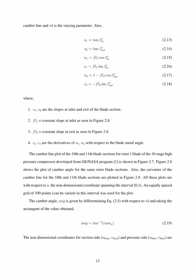
camber line and ub is the varying parameter. Also,

s1 = tan β∗in (2.13)

s2 = tan β∗out (2.14)

u1 = fl1 cos β∗in (2.15)

c1 = fl1 sin β∗in (2.16)

u2 = 1− fl2 cos β∗out (2.17)

c2 = −fl2 sin β∗out (2.18)

where,

1. s1, s2 are the slopes at inlet and exit of the blade section.

2. fl1 = constant slope at inlet as seen in Figure 2.8.

3. fl2 = constant slope at exit as seen in Figure 2.8.

4. c1, c2 are the derivatives of u1, u2 with respect to the blade metal angle.

The camber line plot of the 10th and 11th blade sections for rotor 1 blade of the 10 stage high

pressure compressor developed from GE/NASA program [1] is shown in Figure 2.7. Figure 2.8

shows the plot of camber angle for the same rotor blade sections. Also, the curvature of the

camber line for the 10th and 11th blade sections are plotted in Figure 2.9. All these plots are

with respect to u, the non-dimensional coordinate spanning the interval [0,1]. An equally spaced

grid of 100 points (can be varied) in this interval was used for the plot.

The camber angle, ang is given by differentiating Eq. (2.5) with respect to ub and taking the

arctangent of the value obtained.

ang = tan−1(camu) (2.19)

The non dimensional coordinates for suction side (ubtop, vbtop) and pressure side (ubbot, vbbot) are

13

Figure 2.7: Plot of the camber line of blade sections 10 and 11 of the rotor 1 blade from the 10stage HPC design.

calculated as below:

ubbot = u+ thk sin (ang) (2.20)

vbbot = cam− thk cos (ang) (2.21)

ubtop = u− thk sin (ang) (2.22)

vbtop = cam+ thk cos (ang) (2.23)

where thk is the thickness distribution defined over a non-dimensional unit camber length

(0.0 to 1.0) as given by Wennerstrom [2]. The thickness distribution is described in Figure 2.10

and the nomenclature is as below:

1. x = non-dimensional camber-line length.

2. xT = location of maximum airfoil thickness.

3. t1 = leading edge thickness.

4. T = maximum airfoil thickness.

5. t2 = trailing edge thickness.

6. y1 = airfoil half-thickness upstream of xT .

14

Figure 2.8: Camber angle plot of blade sections 10 and 11 of the rotor 1 blade from the 10 stageHPC design.

7. y2 = airfoil half-thickness downstream of xT .

The thickness equation for x < xT :

y1 = ax3 + bx2 + cx+ d (2.24)

y1′= 3ax2 + 2bx+ c (2.25)

y1′′

= 6ax+ 2b (2.26)

15

Figure 2.9: Plot showing the curvature of the camber line of blade sections 10 and 11 of therotor 1 blade from the 10 stage HPC design.

Figure 2.10: Thickness distribution over a non-dimensional unit camber length [2].

and the thickness equation for x > xT :

y2 = e(x− xT )3 + f(x− xT )2 + g(x− xT ) + h (2.27)

y2′= 3e(x− xT )2 + 2f(x− xT ) + g (2.28)

y2′′

= 6e(x− xT ) + 2f (2.29)

When xT ≥ 0.5, the boundary conditions are:

16

At x = 0

y1 =t12

(2.30)

y1′′

= 0 (2.31)

At x = xT

y1 = y2 =T

2(2.32)

y1′= y2

′= 0 (2.33)

y1′′

= y2′′

(2.34)

At x = 1.0

y2 =t22

(2.35)

(2.36)

From these, the coefficients a through h are derived as explained by the author, Wennerstrom in

his book [2]. When xT < 0.5, the leading and trailing edge boundary conditions are reversed to

obtain the coefficients.

The suction side and pressure side coordinates are merged into a single array of specified

number (199 in this case) of non-dimensional coordinates (ub, vb) respectively, such that the

array starts from the trailing edge and goes counter-clockwise through the leading edge and

comes back to the trailing edge. Since the leading edge and trailing edge coordinates of the

pressure side and suction side are the same, only a single value of the leading edge coordinate

is used in the array and the first and last point in the array is the same trailing edge coordinate.

The non dimensional leading edge is chosen as (0,0) and trailing edge as (1,0) for convenience.

The stagger angle, ζ is calculated by taking the average of the blade metal angles at inlet and

17

exit. The normalized staggered airfoil coordinates (m′bstgr, θbstgr) are as given below:

ζ = (β∗in + β∗out)/2 (2.37)

m′bstgr = ub cos (−ζ) + vb sin (−ζ) (2.38)

θbstgr = −ub sin (−ζ) + vb cos (−ζ) (2.39)

Figure 2.11 shows the airfoil rotated by the stagger angle and is placed on the unit chord on

the non-dimensioanl spacing array system (u, v). chrdx is the non dimensional meridional

chord which is the difference between m′TE and m′LE . The actual chord is calculated and the

airfoil coordinates are scaled by multiplying the staggered coordinates (m′bstgr, θbstgr) with the

non-dimensional actual chord as below:

chrdx = |m′TE −m′LE| (2.40)

chrd = chrdx/ |cos ζ| (2.41)

m′b = m′bstgr(chrd) (2.42)

θb = θbstgr(chrd) (2.43)

Figure 2.11: Blade section on the normalized unit chord.

The resultant 2D blade section contains np values of m′b, θb coordinates in the meridional

coordinate system.

18

2.3.1 Variety of Airfoil shapes

3DBGB is flexibile in its capability of generating different airfoil shapes to cope with a variety

of blade designs. Since each blade section is constructed independently through parameters,

it is possible to have different blade sections at different spanwise locations. For example, a

wind turbine blade has a circular hub and progresses towards an S809 airfoil shape radially.

The general capability of the blade section construction makes it easy to deal with such shapes.

Currently, 3DBGB is capable of generating the S809 airfoil, NACA 4-digit airfoils, a circular

section, and the default airfoil which is a mixed camber airfoil as shown in Figure 2.12. In addi-

tion to these, the tool is flexible in adding various airfoil shapes parametrically. It is recognized

that the default blade section is inadequate for a transonic fan, but those sections can be added

in a parametric fashion. This is also true for many other blade types. The integrated ability for a

general blade section and consistent 3D stacking in a rigorous manner sets this blade generator

apart.

Figure 2.12: Variety of airfoils generated by 3DBGB in addition to circular and 4 digit NACAairfoils.

2.4 Leading Edge and Trailing Edge Curves

The leading and trailing edge are defined by 2D cubic spline curves in x, r. A cubic spline is

used to fit the streamline coordinates xs, rs with m′s as the spline parameter. The intersection of

these curves and the 2D streamline curves produces the leading and trailing edge coordinates

19

(xLE, rLE, xTE, rTE) on the corresponding streamlines. This information is used to obtain the

m′sLE , the leading edge m′s value, which is crucial in streamwise mapping of the blade sections.

2.5 Streamwise Mapping of the Blade Sections

The 2D blade sections created are mapped with their corresponding streamlines. The stream-

lines are defined both upstream and the downstream of the blade for robust mapping. Typical

streamsurfaces are defined by revolving the streamlines about the x-axis. For an axial and radial

machine this is shown in Figure 2.13. m′sLE , the leading edge m′s value is calculated by taking

the inverse spline of x(m′s) evaluated at xLE on each of the streamline as shown in Figure 2.14.

The meridional offset between the blade leading edge m′bLE and the streamline leading edge

Figure 2.13: Stream surface for an axial machine and a radial machine respectively.

Figure 2.14: m′sLE obtained using inverse spline on m′s.

20

m′sLE is calculated and is necessary for precise conformation of the blade section on the corre-

sponding streamline. This is because the zero m′s on each streamline is different from the m′bLE

on each corresponding blade section and this offset is expressed as:

δm′ = m′sLE −m′bLE (2.44)

Similarly, there exists a tangential offset which is added to the θb coordinates to obtain stream-

wise θ3D coordinates for the blade:

θ3D = θb + δθ (2.45)

Once all the offsets are calculated, the streamwise meridional coordinates m′3D for each blade

section is obtained using:

m′3D = m′b + δm′ (2.46)

The m′3D coordinates are used to calculate the streamwise x3D and r3D coordinates by evaluat-

ing the spline at every streamwise meridional coordinate as below:

1. x3D = spline evaluated at each m′3D for all the np points of each blade section.

2. r3D = spline evaluated at each m′3D for all the np points of each blade section.

The spline evaluation process is depicted in Figure 2.15 and Figure 2.16.

Figure 2.15: x3D obtained by spline evaluation at each m′3D of each blade section.

Figure 2.17 shows the mapping of the blade section on the corresponding stream surface.

In this manner, all the blade sections are mapped consistently. x3D, r3D and θ3D coordinates for

21

Figure 2.16: r3D obtained by spline evaluation at each m′3D of each blade section.

Figure 2.17: Mapping of the blade section to the corresponding stream surface.

all the nspn 3D blade sections are thus calculated in the cylindrical coordinate system as shown

in section 2.8.

2.6 Sweep and Lean to the Blade

Spanwise Sweep and Lean are applied as perturbations using a specific number of control points

(span, δm′) and (span, δθ). The control points are used to construct a smooth sweep and lean

definition spanwise using uniform B-splines as explained later in this section. The normalized

22

span of the nth streamline for an axial machine is given by :

Lref = rLETIP − rLEHUB (2.47)

span(n) = r(n)− rHUB (2.48)

˜span(n) = span(n)/(Lref ) (2.49)

where Lref is the blade height.

The sweep perturbation, δm′ values at each streamline are evaluated by interpolating the

δm′ curve at each spanwise location on each streamline as depicted in Figure 2.18. In this

manner, the sweep is added to the blade whenever required. Figure 2.19 shows blades with

forward and backward sweep respectively.

Figure 2.18: δm′ evaluated at each span.

Similarly, the lean is added to the blade as required by defining the lean perturbation with

few control points and obtaining the δθ values at each streamline as explained above. This

method as shown in Figure 2.20 was used to modify the lean near the hub of rotor 3 of the

booster optimum shown as point 2 in the paper by Park et al. [4] to eliminate the corner sep-

aration at the exit which increased the adiabatic efficiency for the isolated blade row 3D CFD

analysis of rotor 3 as explained by Siddappaji et al. [15].

23

Figure 2.19: Forward and backward swept blades respectively.

Figure 2.20: Spanwise lean modification on rotor 3 of a booster optimum resulting in lean nearthe hub.

2.6.1 Construction of Uniform B-Splines

A group of local control points are used to determine the geometry of curve segments which

form a B-spline. A curve segment does not necessarily have to pass through a control point but

its desired at the two end points of the B-spline. Cubic B-splines are popular because of their

continuity characteristics which make the segment joints smooth [3]. Figure 2.21 shows a cubic

curve constructed from a series of curve segments S0, S1, S2, ..., Sm−3,... using m + 1 control

points P0, P1, P2, ..., Pm.

Any single segment Si(t) of a B-spline curve is defined by

Si(t) =3∑r=0

Pi+rBr(t) (2.50)

24

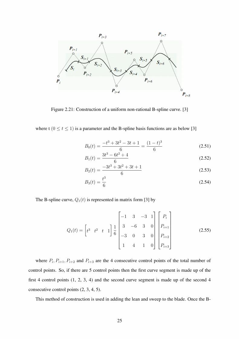
Figure 2.21: Construction of a uniform non-rational B-spline curve. [3]

where t (0 ≤ t ≤ 1) is a parameter and the B-spline basis functions are as below [3]

B0(t) =−t3 + 3t2 − 3t+ 1

6=

(1− t)3

6(2.51)

B1(t) =3t3 − 6t2 + 4

6(2.52)

B2(t) =−3t3 + 3t2 + 3t+ 1

6(2.53)

B3(t) =t3

6(2.54)

The B-spline curve, Q1(t) is represented in matrix form [3] by

Q1(t) =

[t3 t2 t 1

]1

6

−1 3 −3 1

3 −6 3 0

−3 0 3 0

1 4 1 0

Pi

Pi+1

Pi+2

Pi+3

(2.55)

where Pi, Pi+1, Pi+2 and Pi+3 are the 4 consecutive control points of the total number of

control points. So, if there are 5 control points then the first curve segment is made up of the

first 4 control points (1, 2, 3, 4) and the second curve segment is made up of the second 4

consecutive control points (2, 3, 4, 5).

This method of construction is used in adding the lean and sweep to the blade. Once the B-

25

spline is constructed, a simple 2D-curve and a line intersection procedure will give the desired

point on the spline curve. For example, spanwise sweep is defined by the control points (span,

δm′). A B-spline curve of δm′ is constructed as explained above. The δm′ value at a particular

spanwise location is obtained by intersecting the 2D δm′ curve with the line (parallel to X-axis)

passing through that location as shown in Figure 2.18.

2.7 Radial Stacking of 3D Blade Sections

The 3D blade sections are stacked radially by including a θ offset, θstack for each individual

blade section. Stacking is defined as a fraction of the non-dimensional actual chord. This

value is transformed into the average θ3D coordinate, which is subtracted from the array of θ3D

coordinates to obtain the stacking. The stacking can be done at the leading edge, trailing edge,

at any percentage of the chord and at the area centroid of a blade section.

θ3D = θb + δθ + θstack (2.56)

Figure 2.22 explains the theta offset defined for stacking the blade at the leading edge, percent-

age chord and the trailing edge correspondingly. Finally, using the coordinate transformation

the 3D blade coordinates in the cartesian system is obtained for this case.

2.8 Coordinate Transformation

The normal practice is to obtain a 3D blade in the cartesian coordinate system as most of the

CAD packages exist in this system. Therefore a coordinate transformation from the cylindrical

system to the cartesian system is necessary. The engine axis is assumed to be along the X-axis

which makes the x-values remain the same in both coordinate systems.

The transformation is as follows:

26

Figure 2.22: θ offset defined for various stacking option.

x3D = x3D (2.57)

y3D = r3D × sin θ3D (2.58)

z3D = r3D × cos θ3D (2.59)

2.9 Output files

The blade generator code outputs nspn data files, which contain np values of 3D coordinates

for all the nspn blade sections. The number of coordinates in the 3D blade sections are kept the

same as the number of coordinates in the 2D airfoil sections. The 3D blade section files can act

as input files for any CAD package to obtain a 3D Blade CAD model.

27

2.10 3D Blade CAD Model

All the data files are imported in Unigraphics (CAD package) and a lofting procedure is per-

formed to create 3D blade surfaces passing through the blade sections to obtain a smooth 3D

blade as shown in the Figure 2.23. The parameters used in lofting are the 3D spline data ob-

tained as the 3D blade section data from 3DBGB for each blade section .

Figure 2.23: 3D Blade lofted in UG.

2.11 Connecting with CAPRI

CAPRI stands for Computational Analysis PRogramming Interface. The 3D Blade constructed

in UG is a base model and using CAPRI [22, 23], newer blade shapes are obtained by simply

updating the spline information of each 3D blade section on the base model. A simple program

written in C integrates the 3D blade part file and the CAPRI interface through which the spline

update is done and hence the blade geometry is morphed parametrically. The advantage of

using CAPRI is that the geometry data remains in the CAD system and avoids the geometry

translation errors during morphing of the blade geometry.

CAPRI saves significant time and effort in development, deployment, and maintenance of

multi-disciplinary design suites that need to interface with CAD. It does not require low-level

expertise in CAD or CAD programming to use, and provides an intuitive engineering interface

to CAD for MDAO applications.

28

2.12 Extruded Blade

In some cases, grid generators require an extruded blade due to tolerance issues and extrusion

is a property which is useful for other purposes as well. It is achieved through a simple offset

of the hub and the tip streamline coordinates in the normal direction to the streamline. At any

point m′s, the normal in the x-direction, xNORM and the normal in the r-direction, rNORM are

calculated by using the orthogonal property between the normal and the slope at that point.

xNORM =drsdm′s

(2.60)

rNORM = − dxsdm′s

(2.61)

So, the offset in the normal direction as shown in Figure 2.24 is given by

∆n = aLref , (2.62)

where a is the percent offset desired and Lref is the reference length.

Figure 2.24: Offset at the hub streamline.

Also,

∆n = b√xNORM 2 + rNORM 2 (2.63)

where b is an intermediate extruded blade scale factor. b is solved using the 4 equations above,

and the offset at the hub and the tip is obtained as below:

1. streamline coordinates at the hub : xsHUB, rsHUB

29

2. streamline coordinates at the tip : xsTIP , rsTIP

xsExtruded = xsHUB + (b× xNORM) (2.64)

rsExtruded = rsHUB + (b× rNORM) (2.65)

and the offset at the tip as

xsExtruded = xsTIP − (b× xNORM) (2.66)

rsExtruded = rsTIP − (b× rNORM) (2.67)

The new extruded hub and tip streamline coordinates are used instead of the original coordinates

and the blade parameters corresponding to the original hub and tip streamlines are used as the

input to obtain an extruded 3D blade as shown in Figure 2.25 using the procedure as explained

before.

Figure 2.25: Extruded blade at the tip with hub and casing.

30

Chapter 3

CFD Analysis of the 3D blade

A CFD simulation is used to analyze the resulting 3D blade geometry. FINETM/Turbo v8 by

Numeca [24] was used for the 3D CFD analysis on the blade model obtained. FINETM/Turbo

is a high fidelity package which has its own gridding tool, solver and a post processor.

3.1 Gridding

The 3D blade section geometry created along with the hub and the shroud definition was im-

ported into a gridding tool called AutoGrid5 [25]. The blade geometry is the rotor 3 blade of

the 3 stage booster from a paper by Park et. al [4]. The blade model thus imported is given

a tip clearance and other necessary input details such as the rotational speed and type of tur-

bomachinery system. The tip clearance is 0.15% of rotor tip radius which is representative of

a compressor with tight but realistic tip clearance. The grid generated is medium type with

858149 grid points. The flow path is generated and blade to blade mesh is created as shown in

Figure 3.1.

3.2 CFD solver: Euranus

Euranus, the FINETM/Turbo solver is run with inlet boundary conditions of absolute total

pressure, absolute total temperature, spanwise distribution of αx at inlet and φ coming from the

previous blade row and static pressure as the exit boundary condition. An isolated blade row

31

Figure 3.1: Creating the meridional and blade to blade mesh.

32

3D CFD analysis of rotor 3 of the booster optimum shown as point 1 in paper by Park et. al

[4] has been performed. Because of the thick boundary layer of the axisymmetric analysis, the

first displaced streamline was used to define the hub and the last displaced streamline was used

to define the casing. The simulation resulted in an adiabatic efficiency of 91.25% at the design

flow rate. This compares 93.47% from the T-Axi axisymmetric code loss model [17]. Several

runs were made on this case by varying the back pressure to create a speed line (the design mass

flow rate is 92.229 kg/s). Figure 3.2 shows the mass flow rate variation with the total pressure

ratio and Figure 3.3 shows the variation of mass flow rate with the isentropic efficiency and the

wide range of the mass flow rate for the booster can be noticed. Figure 3.4 shows the contour

plot of relative mach numbers from 0.2 to 0.8 on three constant radius cut-planes across rotor

3 of the booster. It also shows stream ribbons across the tip clearance showing the tip vortex.

Reasonable agreement between the axisymmetric and 3D demonstrates how the coupled system

can be used for optimizing a design.

Figure 3.2: Characteristic curve showing Total PR vs mass flow rate.

The isolated blade row 3D CFD analysis of rotor 3 of the booster optimum shown as point

2 in the paper by Park et. al [4] was also performed which resulted in corner separation at the

33

Figure 3.3: Characterisitic curve showing Isentropic efficiency vs mass flow rate.

Figure 3.4: Relative Mach contours of rotor 3 of the optimized booster with stream ribbons atover the tip clearance.

34

exit with an adiabatic efficiency of 93.17%. The lean of the 3D blade geometry was modified as

shown in Figure 3.5 which eliminated the separation near the exit as shown in Figure 3.6 which

is the comparison of the iso surface of axial velocity for the original and modified rotor 3 for

this case. The adiabatic efficiency increased to 93.93%. This compares to the T-Axi efficiency

of 95.27% for this rotor. It should be noted that this is still not an optimum. The shape shows

that there might be stress issues except that the wheel speed is so low which is why the coupling

with a finite element structural solver is so important.

Figure 3.5: Spanwise lean modification on rotor 3.

Figure 3.6: Iso surface comparison of axial velocity for original and modified rotor 3 of thebooster optimum point 2 [4].

35

Chapter 4

Structural Analysis of the 3D Blade

Structural Analysis is a critical design simulation capability and its use is demonstrated on the

blade geometry. ANSYS V12.0 [26] is used. A CAD part file of the 3D blade model is imported

and a script file called ’Blade.ain’ is used which contains the material properties of the blade

and also the instructions for meshing the blade. This creates a meshed blade with hexagonal

mesh as shown in Figure 4.1 and is ready for structural analysis. The blade model used is the

rotor 1 blade of the 10 stage High Pressure Compressor. A modal analysis is performed with 14

modes and the procedure is as follows:

• Analysis type is defined.

Solution→ Analysis Type→ New Analysis→Modal.

• Analysis option is set.

Solution→Analysis Type→Analysis Options→ Preconditioned Conjugate Gradient (PCG)

Lanczos.

• Number of modes to extract is 14 and it extracts modes for all Degrees Of Freedoms

(DOF’s).

• Constraints are applied.

Solution→ Define Loads→ Apply→ Structural→ Displacement→ On Areas.

• The hub area of the blade is selected.

36

Figure 4.1: Blade meshed in ANSYS V12.0.

• The system is solved.

Solution→ Solve→ Current Load Step (LS).

After the solution is complete post processing is performed. Figures 4.2 and 4.3 shows

the contour plots of the Displacement vector sum of Degrees Of Freedom (DOF) solution under

Nodal solution for all the 14 modes of the blade. The plots are of a deformed shape of the blade.

Figure 4.2: Contour plots of Displacement vector sum for first 7 modes of a blade under Nodalsolution.

37

Figure 4.3: Contour plots of Displacement vector sum for last 7 modes of a blade under Nodalsolution.

Also, Figure 4.4 shows the displaced blade with the undisplaced blade shape keeping the

hub of the blade fixed. This completes the structural analysis of the blade.

Figure 4.4: Displaced blade.

38

Chapter 5

Example Design Problems

The capability of the 3DBGB is demonstrated through the following examples. The examples

include a 10 stage EEE high pressure compressor design, a 3 stage booster, a low speed centrifu-

gal compressor, all of which are generated using the design data from reports. A wind turbine

design is also demonstrated, and has been reverse engineered from pictures, marketing literature

[6] and a report [27]. All these example cases are available at http://gtsl.ase.uc.edu/3DBGB/.

5.1 10 Stage EEE High Pressure Compressor Design

The GE Energy Efficient Engine (E3) high pressure compressor (HPC) as shown in Figure 5.1

was used as an example, which has 21 blade rows with 10 stages and an IGV. Two cases were

generated, one with free vortex having straight leading and trailing edges and the other with full

definition of spanwise angular momentum having non-straight leading and trailing edges.

5.1.1 Free vortex Design

|

The angular momentum is kept constant along the blade span for all the blade rows for

this case and it has straight leading and trailing edges. The input files for running T-Axi (ax-

isymmetric solver) [16, 17, 18, 19] for this case are available on the T-Axi website[16] under

input.zip/T-AXI Input Files/EEE-HPC-des. The axisymmetric grid of this 10 stage HPC (free

vortex) is shown in Figure 5.2. The grid is created by the hub and casing definitions used in

39

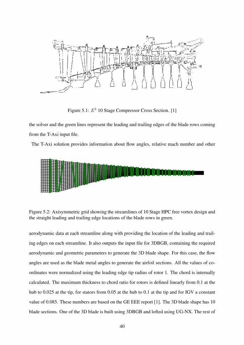
Figure 5.1: E3 10 Stage Compressor Cross Section. [1]

the solver and the green lines represent the leading and trailing edges of the blade rows coming

from the T-Axi input file.

The T-Axi solution provides information about flow angles, relative mach number and other

Figure 5.2: Axisymmetric grid showing the streamlines of 10 Stage HPC free vortex design andthe straight leading and trailing edge locations of the blade rows in green.

aerodynamic data at each streamline along with providing the location of the leading and trail-

ing edges on each streamline. It also outputs the input file for 3DBGB, containing the required

aerodynamic and geometric parameters to generate the 3D blade shape. For this case, the flow

angles are used as the blade metal angles to generate the airfoil sections. All the values of co-

ordinates were normalized using the leading edge tip radius of rotor 1. The chord is internally

calculated. The maximum thickness to chord ratio for rotors is defined linearly from 0.1 at the

hub to 0.025 at the tip, for stators from 0.05 at the hub to 0.1 at the tip and for IGV a constant

value of 0.085. These numbers are based on the GE EEE report [1]. The 3D blade shape has 10

blade sections. One of the 3D blade is built using 3DBGB and lofted using UG-NX. The rest of

40

the blades are obtained by updating the spline data on the initial blade using CAPRI [22, 23].

The spline data is produced as 3D blade section data for the respective blades by 3DBGB. The

blades are stacked at their leading edge for this case. The rotor 1 and rotor 3 blade shapes for

the free vortex design are shown in Figure 5.3.

Figure 5.3: Rotor 1 and rotor 3 of EEE HPC free vortex design created using 3DBGB.

In this manner, all the 21 blade rows are constructed and are assembled with their corre-

sponding disks optimized with T-Axi Disk [5, 20] to obtain blisks. Rotor 1 and rotor 3 blisks

are shown in Figure 5.4.

41

Figure 5.4: Rotor 1 and Rotor 3 blisk assembly for EEE HPC free vortex design.

42

5.1.2 Full Definition 10 stage Design

The angular momentum along the blade span is not constant for the E3 case and it has non-

straight leading and trailing edges. The input files for running T-Axi for this case are available

on the T-Axi website [16] under input.zip/T-AXI Input Files/EEE-HPC-analyse. The axisym-

metric grid of the GE EEE HPC (full definition) is shown in Figure 5.5. The grid is created by

the hub and casing definitions used in the solver and the green lines represent the leading and

trailing edges of the blade rows coming from the T-Axi input file.

Figure 5.5: Axisymmetric grid showing the streamlines of E3 10 Stage HPC full definitiondesign and the leading and trailing edge locations of the blade rows in green.

The T-Axi solution gives flow angles and other aerodynamic data for all the specified 21

streamlines and also outputs 3DBGB input containing required information for 21 streamlines.

For this case, the blade metal angles from the NASA report[1] were used to construct the airfoil

sections. The NASA report contains data tables of blade metal angles, maximum thickness

to chord ratio and other parameters tabulated spanwise for all 21 bladerows of the GE EEE

High Pressure Compressor. The report has data tabulated at 12 spanwise locations for each

blade. These 12 values of the blade metal angles and the maximum thickness to chord ratio

were interpolated to 21 values since this 3DBGB input has 21 spanwise locations. All the

values of coordinates were normalized using the leading edge tip radius of rotor 1. A spanwise

comparison of the 12 values of blade metal angles (β∗1 , β∗2) at inlet and exit of rotor 3 as given

in the NASA report [1] with 21 interpolated values obtained by 3DBGB is shown in Figure 5.6.

Using these interpolated values and the internally calculated leading and trailing edge locations,

a 3D blade shape with non-straight leading and trailing edge is constructed for rotor 3 in this

case and is shown in Figure 5.7. The first 5 rotors were stacked at the center of the 2D airfoil

43

Figure 5.6: Comparison of blade metal angles of EEE-HPC rotor 3 given in the report [1] andgenerated by 3DBGB.

area and the rest were stacked at quarter chord radially. All the other 20 blades are constructed

using CAPRI and respective spline data as explained before. A complete assembly with all the

10 rotors, 10 stators and the IGV is created in UG without the hub and the casing definition and

is shown in Figure 5.8.

Figure 5.7: Rotor 3 of GE EEE HPC full definition design with non-straight leading and trailingedges.

44

Figure 5.8: Rotor and stator assembly for 10 stage HPC full definition design from the GE/E3

parameters.

45

5.2 3 Stage Booster Design for Turbofan Engine

A 3 stage booster for a turbofan engine (CFM56 class machine) was designed. Boosters are

used in turbofan engines before the high pressure compressor. The 3 stage booster of the GE90

turbofan engine shown in Figure 5.9 depicts where the boosters are used.

Figure 5.9: 3 stage booster of a GE90 turbofan engine.[5]

A 3 stage booster flow path geometry along with the blades was optimized as explained in

the paper by Park et. al [4] and the best result was used for generating 3D blades. The ax-

isymmetric grid of the optimized booster is shown in Figure 5.10 which shows the streamlines

calculated by T-Axi and the leading and trailing edges of blade rows in green lines. The axisym-

metric solver (T-Axi) is run and the input for 3DBGB was obtained. The flow angles are used as

the blade metal angles for the 2D airfoils construction. The maximum thickness to chord ratio

for rotors is defined linearly from 0.1 at the hub to 0.025 at the tip and for stators from 0.05 at

the hub to 0.1 at the tip. All the blade rows are created as explained in the previous example

and the rotors and stators are assembled as shown in Figures 5.11 and 5.12.

The validation of rotor 3 was done by performing a 3D-CFD analysis which is explained in

Chapter 3. The FEA structural analysis was also performed on rotor 3 with a tetrahedral mesh

as shown in Figure 5.13. A modal analysis on the blade resulted in 14 modal shapes and the

46

Figure 5.10: Axisymmetric grid of the 3-stage optimized booster showing the streamlines andthe leading and trailing edge locations of the blade rows in green.

Figure 5.11: 3 stage booster rotor assembly with the fan blades.

47

Figure 5.12: 3 stage booster assembly with split casing.

48

contour plots of the displacement vector sum is shown in Figure 5.14.

Figure 5.13: Tetrahedral mesh of rotor 3 of a 3 stage booster in ANSYS.

Figure 5.14: Contour plots of displacement vector sum of all 14 modes of rotor 3 under Modalsolution.

49

5.3 Reverse-Engineered Wind Turbine Design

Wind turbines can be treated as turbines without the nozzle. All the turbomachinery principles

apply to them. 3DBGB is capable of creating wind turbine blades due to its generality. This

capability is demonstrated by building the reverse engineered GE 1.5 MW wind turbine blade as

shown in Figure 5.15. Pictures, marketing literature [6] and a report [27] were used for reverse

engineering.

Figure 5.15: GE 1.5 MW wind turbine blade. [6]

The case for T-Axi was set up as explained in the Masters thesis by Dey [28]. The axisym-

metric grid of the reverse engineered GE wind turbine blade is shown in Figure 5.16. The wind

turbine was treated as a half stage turbine with extended tip in T-Axi solver. T-Axi generates the

input for 3DBGB and the wind turbine 3D blade geometry is created as shown in Figure 5.17. It

is then assembled with the bullet nose and a wind turbine model with 3 blades is created using

UniGraphics as shown in Figure 5.18. While generating a similar wind turbine blade shape,

one of the issues encountered was going beyond axial (ζ equal to 92 degrees), where the blade

shapes failed to be generated since the chrd value calculated according to the Eq.(2.41) became

a non-defined value as cosine of the stagger angle reaches zero. To overcome this issue, a switch

was added in the input file which would read the actual non-dimensional chord values chrd for

such high staggered cases instead of using Eq.(2.41). The addition of this option expands the

capability of the tool to include blades with very high stagger.

The utility of the blade generation is demonstrated by performing CFD analysis as explained

in the Masters thesis by Dey [28]. FEA structural analysis was also performed by treating the

blade as a rotating cantilever beam. The meshed blade has 8 node hexahedron brick 185 element

50

Figure 5.16: Axisymmetric grid of the reverse engineered GE 1.5 MW wind turbine blade.

Figure 5.17: Reverse engineered GE 1.5 MW wind turbine blade geometry created using3DBGB.

51

Figure 5.18: Reverse Engineered GE 1.5 MW wind turbine assembly.

52

as shown in Figure 5.19. Structural analysis was executed and the Von-Mises plot is shown in

Figure 5.20. Aluminium material was used for the blade which has the yield strength of 414

MPa. The maximum value of the von-mises stress obtained was 47.417 MPa, which is less than

one third times the yield strength.

Figure 5.19: Meshed wind-turbine blade with 8 node Hexahedron Brick 185 element.

Figure 5.20: Von-Mises Stress plot on GE reverse engineered blade.

The first 5 mode shapes for the reverse engineered GE wind turbine blade is shown in

Figure 5.21.

53

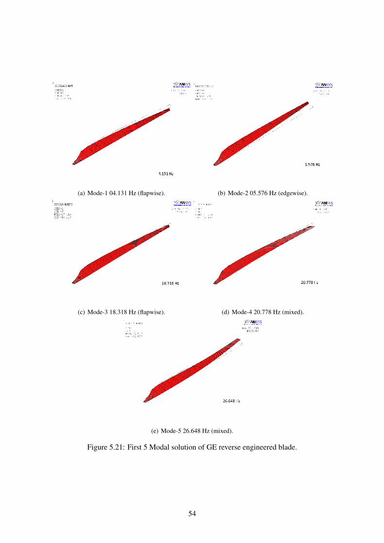
(a) Mode-1 04.131 Hz (flapwise). (b) Mode-2 05.576 Hz (edgewise).

(c) Mode-3 18.318 Hz (flapwise). (d) Mode-4 20.778 Hz (mixed).

(e) Mode-5 26.648 Hz (mixed).

Figure 5.21: First 5 Modal solution of GE reverse engineered blade.

54

5.4 Low-Speed Centrifugal Compressor design

3DBGB is also capable of designing 3D blades for radial machines. The low-speed centrifugal

compressor (LSCC) blade model is generated as an example case. The compressor is based on a

NASA design [7] and has 20 blades with the speed of 1862 rpm. The flowpath of the compressor

with the actual experimental setup measurements is shown in Figure 5.22. Figure 5.23 shows

the radial grid of the compressor with hub and casing definition and the streamlines along with

leading edge and trailing edge locations denoted by green lines.

Figure 5.22: LSCC flowpath with actual measurements. [7]

The NASA report [7] contains hub and tip streamline coordinates and other airfoil geometry

data. The hub and tip flowpath were linearly interpolated in the radial direction to generate more

construction lines. A total number of 5 construction lines including the hub and tip streamlines

were generated. All the coordinates were normalized with the leading edge tip radius value.

The inlet was treated to be purely axial with constant axial velocity, Vz. The wheel speed at the

tip, Ut is given to be 153 m/s. The report had spanwise plots of VzUt

ratios and an average value

of 0.4 at 50% pitch was used to calculate the constant axial velocity as 61.2 m/s. Figure 5.24

shows the velocity triangle for the purely axial flow at the leading edge, where the relative flow

angles at the leading edge for different spans are calculated as below:

55

Figure 5.23: A radial compressor flowpath showing the hub and casing with streamlines andthe leading and trailing edge locations.

1. Vz = Axial flow velocity.

2. U = Wheel speed.

3. N = Wheel rotational speed in RPM.

4. W = Relative flow velocity = U = ωr.

5. r = radius in meters.

6. ω = 2πN60

7. Wθ = Tangential relative flow velocity.

8. βz = Relative flow angle = tan−1 Wθ

Vz.

The outlet was treated to be purely radial with constant relative flow angle of 55o spanwise.

The design methodology used to create axial blades was applied except, the blade was stacked at

the trailing edge. Also, a condition was added to check the slope of the streamline to distinguish

between radial and axial machines. When,

∣∣∣∣ drsdm′s

∣∣∣∣ > ∣∣∣∣ dxsdm′s

∣∣∣∣ (5.1)

56

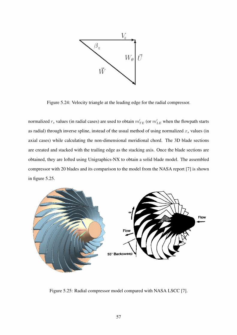
Figure 5.24: Velocity triangle at the leading edge for the radial compressor.

normalized rs values (in radial cases) are used to obtain m′TE (or m′LE when the flowpath starts

as radial) through inverse spline, instead of the usual method of using normalized xs values (in

axial cases) while calculating the non-dimensional meridional chord. The 3D blade sections

are created and stacked with the trailing edge as the stacking axis. Once the blade sections are

obtained, they are lofted using Unigraphics-NX to obtain a solid blade model. The assembled

compressor with 20 blades and its comparison to the model from the NASA report [7] is shown

in figure 5.25.

Figure 5.25: Radial compressor model compared with NASA LSCC [7].

57

Chapter 6

Conclusion and Future Work

6.1 Conclusion

The development of a parametric 3D blade geometry modeling tool for turbomachinery has been

presented. The tool is capable of generating a specified number of data files containing np coor-

dinates of 3D blade sections based on very few geometric and aerodynamic parameters. The 3D

blade sections can be imported into a CAD package to obtain a smooth lofted blade. The geom-

etry modification process is made quicker and easier by the parametric definition of the splines.

The benefits of this new method are a large design space including many stacking options with a

small number of parameters. The flexibility of the tool has been demonstrated by locally modi-

fying the lean in the hub of rotor 3 of a 3-stage booster for turbofan engine to eliminate a corner

separation. The geometry tool and the demonstrated connection of this tool to a CFD code and

FEA code is part of a complete high fidelity design system. The capability to create 3D blades

for various types of turbomachinery has demonstrated the generality of the approach through

various example cases. The utility of the 3D blade geometry generation is demonstrated by per-

forming a 3D-CFD analysis and an FEA structural analysis on the obtained blade shape. The

flexibility and generality of the tool is also demonstrated through the examples. The executable

that creates the 3D blades is freely available at http://gtsl.ase.uc.edu/3DBGB/ along with the

example cases.

58

6.2 Future Work

The tool is ready for adding many other capabilities which will make it more general and robust.

The parametrization of the camber and thickness distribution will make designing of transonic

airfoils possible. Future work also includes more options for blade sections and defining the 2D

blade sections parametrically as a combination of many different sections. Also, this tool can

be tied to an optimizer to obtain optimized 3D blade geometries. 3DBGB can really grow into

a powerful and an extremely flexible geometry generator.

59

References

[1] Holloway, P., Knight, G., Koch, C., and Shaffer, S., 1982. Energy efficient engine high

pressure compressor detail design report. Tech. rep., General Electric Company, NASA-

CR-165558.

[2] Wennerstrom, A. J., 2000. Design of Highly Loaded Axial-flow Fans and Compressors.

Concepts ETI, Inc., Vermont.

[3] Vince, J., 2006. Mathematics for Computer Graphics 2nd Edition. Springer, New Jersey.

[4] Park, K., Turner, M. G., Siddappaji, K., Dey, S., and Merchant, A., 2011. “Optimization

of a 3-stage booster part 1: The axisymmetric multi-disciplinary optimization approach to

compressor design”. ASME Paper Number GT2011-46569.

[5] Gutzwiller, D. P., 2009. “Automated design, analysis, and optimization of turbomachinery

disks”. Master’s thesis, University of Cincinnati, Cincinnati, OH, September.

[6] GE-Power. http://www.gepower.com/prod\_serv/products/wind\

_turbines/en/15mw/index.htm.

[7] Hathaway, M. D., Chriss, R. M., Strazisar, A. J., and Wood, J. R., 1995. Laser anemometer

measurements of the three-dimensional rotor flow field in the nasa low-speed centrifugal

compressor. Tech. rep., NASA ARL-TR-333.

[8] Grasel, J., Keskin, A., Swoboda, M., Przewozny, H., and Saxer, A., 2004. “A full para-

metric model for turbomachinery blade design and optimisation”. DETC Paper Number

DETC2004-57467.

60

[9] Dutta, A. K., Flassig, P. M., and bestle, D., 2008. “A non-dimensional quasi-3d blade

design approach with respect to aerodynamic criteria”. ASME Paper Number GT2008-

50687.

[10] Koini, G. N., Sarakinos, S. S., and Nikolos, I. K., 2009. “A software tool for paramet-

ric design of turbomachinery blades”. Advances in Engineering Software, 40, January,

pp. 41–51.

[11] Korakianitis, T., 1993. “Prescribed-curvature-distribution airfoils for the preliminary geo-

metric design of axial turbomachinery cascades”. ASME Journal of Turbomachinery, 115,

April, pp. 325–333.

[12] Anders, J. M., Haarmeyer, J., and Heukenkamp, H., 1999. “A parametric blade design

system (part 1 + 2)”. In Von Karman Institute for fluid dynamics: lecture series 1999-

2002 turbomachinery blade design systems.

[13] IV, P. L. M., Oliver, J. H., Miller, D. P., and Tweet, D. L., 1996. “Bladecad: An interactive

geometric design tool for turbomachinery blades”. 41st Gas Turbine and Aeroengine

Congress sponsored by ASME, NASA Technical Memorandum 107262.

[14] NASA Research Announcement NNNC07CB61C-06-SSFW2-06-0071, Advanced De-

sign Techniques for MDAO of Turbomachinery with Emphasis for the Engine System.

[15] Siddappaji, K., Turner, M. G., Dey, S., Park, K., and Merchant, A., 2011. “Optimization

of a 3-stage booster- part 2: The parametric 3d blade geometry modeling tool”. ASME

Paper Number GT2011-46664.

[16] University of Cincinnati T-Axi Website http://gtsl.ase.uc.edu/T-AXI/.

[17] Turner, M. G., Merchant, A., and Bruna, D., 2006. “A turbomachinery design tool for

teaching design concepts for axial-flow fans, compressors, and turbines”. ASME Paper

Number GT2006-90105.

[18] Turner, M. G., Bruna, D., and Merchant, A., 2007. “Applications of a turbomachinery

design tool for compressors and turbines”. AIAA Paper Number 2007-5152.

61

[19] Bruna, D., Cravero, C., Turner, M. G., and Merchant, A., 2007. “An educational software

suite for teaching design strategies for multistage axial flow compressors”. ASME Paper

Number GT2007-27160.

[20] Gutzwiller, D. P., Turner, M. G., and Downing, M. J., 2009. “Educational software for

blade and disk design”. ASME Paper Number GT2009-59692.

[21] Goodhand, M. N., and Miller, R. J., 2010. “The impact of real geometries on three-

dimensional separations in compressors”. ASME Paper Number GT2010-22246.

[22] Haimes, R., and Follen, G. J., 1998. “Computational analysis programming interface”. 6th

International Conference on Numerical grid generation in computational field simulations.

[23] Merchant, A., and Haimes, R., 2003. “A cad-based blade geometry model for turboma-

chinery aero design systems”. In GT-2003-38305.

[24] NUMECA International. FINE/Turbo http://numeca.be/index.php?id=16.

[25] NUMECA International. Autogrid http://numeca.be/index.php?id=25.

[26] ANSYS Inc. www.ansys.com/products/Workflow+Technology.

[27] A.Griffin, D. Tech. rep., Global Energy Concepts,LLC, Washington,USA. SAND2002-

1879.

[28] Dey, S., 2011. “Wind turbine blade design system - aerodynamic and structural analysis”.

Master’s thesis, University of Cincinnati, Cincinnati, OH, May.

62

Appendix A

Input Files for Example Cases

A.1 Rotor 3 of 10 Stage EEE HPC Free Vortex Design

63

Input parameters (version 1 . 0 )

e3c−des

Blade row # :

6

Number of blades in this row :

50

Blade Scaling factor (mm ) :

350.700000000000

Number of streamlines :

21

Non−dimensional Actual chord (0=no , 1=yes ) :

0

J in_Beta out_Beta mrel_in chord t /c_max Incidence Deviation Sec . Flow Angle

1 −54.45378568 −34.39556205 0 .83674931 0 .14516934 0 .10000000 0 .00000000 0 .00000000 0 .00000000

2 −55.14168979 −35.61221762 0 .84411465 0 .14191943 0 .09625000 0 .00000000 0 .00000000 0 .00000000

3 −55.82137412 −36.65746602 0 .85230672 0 .13871866 0 .09250000 0 .00000000 0 .00000000 0 .00000000

4 −56.45007999 −38.03929806 0 .86180055 0 .13540971 0 .08875000 0 .00000000 0 .00000000 0 .00000000

5 −57.10874871 −39.44286108 0 .87366224 0 .13191032 0 .08500000 0 .00000000 0 .00000000 0 .00000000

6 −57.64493298 −40.71282164 0 .88426519 0 .12861769 0 .08125000 0 .00000000 0 .00000000 0 .00000000

7 −58.11412665 −41.99550525 0 .89502469 0 .12533620 0 .07750000 0 .00000000 0 .00000000 0 .00000000

8 −58.61624717 −43.28572053 0 .90780043 0 .12207390 0 .07375000 0 .00000000 0 .00000000 0 .00000000

9 −59.07111963 −44.53789880 0 .92071561 0 .11883727 0 .07000000 0 .00000000 0 .00000000 0 .00000000

10 −59.48807345 −45.71110426 0 .93380343 0 .11563147 0 .06625000 0 .00000000 0 .00000000 0 .00000000

11 −59.90159667 −46.94121033 0 .94713464 0 .11246059 0 .06250000 0 .00000000 0 .00000000 0 .00000000

12 −60.31118168 −48.05673163 0 .96134154 0 .10932787 0 .05875000 0 .00000000 0 .00000000 0 .00000000

13 −60.69878423 −49.16722571 0 .97579120 0 .10623587 0 .05500000 0 .00000000 0 .00000000 0 .00000000

14 −61.06564215 −50.19665595 0 .98960204 0 .10319161 0 .05125000 0 .00000000 0 .00000000 0 .00000000

15 −61.45947417 −51.22287760 1 .00527050 0 .10017988 0 .04750000 0 .00000000 0 .00000000 0 .00000000

16 −61.83652305 −52.21555570 1 .02005852 0 .09721474 0 .04375000 0 .00000000 0 .00000000 0 .00000000

17 −62.21836349 −53.11690457 1 .03477831 0 .09429861 0 .04000000 0 .00000000 0 .00000000 0 .00000000

18 −62.62239995 −53.91798953 1 .05017808 0 .09143510 0 .03625000 0 .00000000 0 .00000000 0 .00000000

19 −63.08901141 −54.67551014 1 .06535098 0 .08863005 0 .03250000 0 .00000000 0 .00000000 0 .00000000

20 −63.60623898 −55.35913372 1 .07943082 0 .08589361 0 .02875000 0 .00000000 0 .00000000 0 .00000000

21 −64.13495390 −55.94734533 1 .09180298 0 .08324520 0 .02500000 0 .00000000 0 .00000000 0 .00000000

LE / TE curve (x ,r ) definition :

Number of Curve points :

2

64

xLE rLE xTE rTE

0 .91899200 0 .70675600 1 .02250000 0 .72333900

0 .93725400 0 .94021300 1 .01388300 0 .93371600

Airfoil type{bf1 (sect1 ) + bf2 (sect2 ) + . . . } :

J type

1 sect1

2 sect1

3 sect1

4 sect1

5 sect1

6 sect1

7 sect1

8 sect1

9 sect1

10 sect1

11 sect1

12 sect1

13 sect1

14 sect1

15 sect1

16 sect1

17 sect1

18 sect1

19 sect1

20 sect1

21 sect1

Control table for blending section variable :

5 0 0

span bf1 bf2

0.000000000000000E+000 1 0

0.250000000000000 1 0

0.500000000000000 1 0

0.750000000000000 1 0

1.00000000000000 1 0

Stacking axis as a fraction of chord ( 2 . =centroid ) :

0 . 2 5

65

Control points for delta_m :

5

span delta_m

0.000000000000000E+000 0.000000000000000E+000

0.250000000000000 0.000000000000000E+000

0.500000000000000 0.000000000000000E+000

0.750000000000000 0.000000000000000E+000

1.00000000000000 0.000000000000000E+000

Control points for delta_theta :

5

span delta_theta

0.000000000000000E+000 0.000000000000000E+000

0.250000000000000 0.000000000000000E+000

0.500000000000000 0.000000000000000E+000

0.750000000000000 0.000000000000000E+000

1.00000000000000 0.000000000000000E+000

Control points for in_beta* :

5

span in_beta*

0.000000000000000E+000 0.000000000000000E+000

0.250000000000000 0.000000000000000E+000

0.500000000000000 0.000000000000000E+000

0.750000000000000 0.000000000000000E+000

1.00000000000000 0.000000000000000E+000

Control points for out_beta* :

5

span out_beta*

0.000000000000000E+000 0.000000000000000E+000

0.250000000000000 0.000000000000000E+000

0.500000000000000 0.000000000000000E+000

0.750000000000000 0.000000000000000E+000

1.00000000000000 0.000000000000000E+000

Control points for chord :

5

66

span chord

0.000000000000000E+000 0.000000000000000E+000

0.250000000000000 0.000000000000000E+000

0.500000000000000 0.000000000000000E+000

0.750000000000000 0.000000000000000E+000

1.00000000000000 0.000000000000000E+000

Control points for tm /c :

5

span tm /c

0.000000000000000E+000 0.000000000000000E+000

0.250000000000000 0.000000000000000E+000

0.500000000000000 0.000000000000000E+000

0.750000000000000 0.000000000000000E+000

1.00000000000000 0.000000000000000E+000

Hub offset

0.000000000000000E+000

Tip offset

0.000000000000000E+000

Streamline Data

x_s r_s

−0.300000000000000 0.492475000000000

−0.200000000000000 0.492475000000000

−0.100000000000000 0.492475000000000

−5.000000000000000E−002 0.492475000000000

0.000000000000000E+000 0.492475000000000

6.640000000000000E−004 0.492545000000000

0.100306000000000 0.503049000000000

0.140864000000000 0.507324000000000

0.422865000000000 0.583169000000000

0.456012000000000 0.592084000000000

0.570901000000000 0.622984000000000

0.608699000000000 0.633150000000000

0.760491000000000 0.671114000000000

0.806337000000000 0.682580000000000

0.889386000000000 0.703351000000000

0.918992000000000 0.710756000000000

67

1.02250000000000 0.727339000000000

1.06183400000000 0.733641000000000

1.13265500000000 0.744987000000000

1.16505200000000 0.750178000000000

1.24483500000000 0.757601000000000

1.28248100000000 0.761104000000000

1.34497700000000 0.766919000000000

1.37353300000000 0.769577000000000

1.43689600000000 0.770937000000000

1.46249900000000 0.771486000000000

1.51795200000000 0.772677000000000

1.56858900000000 0.773763000000000

1.62055600000000 0.775954000000000

1.64641300000000 0.777043000000000

1.70237400000000 0.779402000000000

1.72838100000000 0.780498000000000

1.78114700000000 0.780206000000000

1.80915200000000 0.780050000000000

1.86586300000000 0.779736000000000

1.91677400000000 0.779454000000000

1.96782300000000 0.780179000000000

1.99820500000000 0.780610000000000

2.05502500000000 0.781416000000000

2.08450500000000 0.781834000000000

2.13184700000000 0.781235000000000

2.16284600000000 0.780843000000000

2.21513700000000 0.780180000000000

2.24599000000000 0.779790000000000

2.28900500000000 0.780295000000000

2.32042700000000 0.780664000000000

2.37099600000000 0.781258000000000

2.39886900000000 0.781586000000000

2.44886900000000 0.781586000000000

2.49886900000000 0.781586000000000

2.59886900000000 0.781586000000000

2.69886900000000 0.781586000000000

0 0

0.887027885345457 0.714158560015747

0.898121204156214 0.716613437507956

68

0.909227551237750 0.718994592353480

0.920358329740695 0.721263142568342

0.931524449485138 0.723394872581633

0.942729760476537 0.725416162343746

0.953972302161670 0.727372105706888

0.965246876184555 0.729280883009763

0.976546163726705 0.731138126989663

0.987861464567192 0.732927628357163

0.999183338646702 0.734637422762338

1.01050230179137 0.736272391963223

1.02180987190148 0.737857199609050

1.03310127869830 0.739430202208498

1.04438004942671 0.741019033039606

1.05565265737710 0.742630404827388

1.06692520102676 0.744277707429729

0 0

0.887530786012880 0.723953914765393

0.898647988484292 0.726174002744471

0.909779116071509 0.728324640841682

0.920929453701887 0.730383117696121

0.932105692995070 0.732334715314499

0.943312714056185 0.734206259638705

0.954550606189579 0.736039687746519

0.965815984561839 0.737847451966079

0.977103121336275 0.739616776559897

0.988404790604791 0.741323920642173

0.999713032885463 0.742951917695323

1.01101999550058 0.744502589924324

1.02231906498525 0.745998056966711

1.03360687736118 0.747475567279002

1.04488576751362 0.748962621778329

1.05616009805065 0.750470664572624

0 0

0.888055772231440 0.733993008879992

0.899192691495258 0.735990273604496

0.910342738872589 0.737928399820692

0.921507732919570 0.739792242755987

0.932692179518577 0.741572454114179

0.943901175520140 0.743296545682390

69

0.955135928640186 0.745004850928974

0.966394343109894 0.746704978017070

0.977671985414048 0.748377188091378

0.988962914613382 0.749991216865181

1.00026047745635 0.751525401643972

1.01155816560762 0.752978904593823

1.02285062568079 0.754373291572454

1.03413513729183 0.755746045241440

1.04541332464835 0.757125659842511

1.05668821762825 0.758523590971057

0 0

0.899752041834668 0.746048568086788

0.910917028672683 0.747787442762525

0.922093533498067 0.749468192216781

0.933284831390208 0.751082918741596

0.944495988693739 0.752659827980109

0.955728848696631 0.754239909319875

0.966982227765011 0.755825988646962

0.978252714968684 0.757392611758612

0.989535438058985 0.758903792182033

1.00082482757861 0.760333722017034

1.01211541858327 0.761679712589621

1.02340270310220 0.762963970320697

1.03468429287106 0.764224576092222

1.04596138792137 0.765490252869619

1.05723619903728 0.766771195086638

0 0

0.900323941984663 0.756335304437585

0.911501153377962 0.757885462244486

0.922687113542332 0.759391266393577

0.933884362389418 0.760848912091724

0.945097885780166 0.762285139093301

0.956329911501288 0.763736536092733

0.967579906441835 0.765202582791977

0.978845250737930 0.766653463100314

0.990121928096028 0.768049472096731

1.00140523037463 0.769362595293850

1.01269047998140 0.770589844142177

1.02397375089723 0.771755060716253

70

1.03525286087564 0.772896645800766

1.04652876966312 0.774042297242936

1.05780319915467 0.775200452466180

0 0

0.900907021728567 0.766839591902578

0.912094604408319 0.768209242897784

0.923288677867156 0.769547000468173

0.934491326614849 0.770850414348401

0.945707466821370 0.772144767409042

0.956939576266779 0.773464308896631

0.968187591255606 0.774805135235913

0.979449494472620 0.776133681565170

0.990721936105404 0.777406966233100

1.00200087371866 0.778595262497818

1.01328221837250 0.779695923336508

1.02456246053798 0.780735099164639

1.03583957262450 0.781751690486626

1.04711439410175 0.782772005322957

1.05838836665390 0.783802824332952

0 0

0.901500369203350 0.777553487471240

0.912697067129929 0.778749247866209

0.923898394929159 0.779923551381090

0.935106149019358 0.781074675019252

0.946325199211879 0.782226518075019

0.957558196813384 0.783411359460293

0.968805420564116 0.784622381307286

0.980065307073955 0.785822599227095

0.991335015496409 0.786966204549945

1.00261100975076 0.788022307014097

1.01388964175513 0.788989257779112

1.02516771223241 0.789896214110991

1.03644332536149 0.790782722643516

1.04771727705927 0.791673313269174

1.05899085865673 0.792573313557684

0 0

0.902103365881728 0.788471903425610

0.913308343679915 0.789498795531759

0.924516400250428 0.790512981711744

71

0.935729147390743 0.791513135449572

0.946951429106921 0.792521788053461

0.958186023088509 0.793569360126700

0.969433460021625 0.794646372690337

0.980692516132532 0.795712731022275

0.991960734766012 0.796720215050946

1.00323496230057 0.797637339240838

1.01451188339638 0.798464133135123

1.02578853787510 0.799233483161924

1.03706314837199 0.799985685419341

1.04833651411984 0.800743043980159

1.05960985535918 0.801509603622146

0 0

0.902715583206547 0.799592066081638

0.913928305413466 0.800454024842128

0.925142797319818 0.801310513695796

0.936360551092840 0.802160480165959

0.947586399278979 0.803025094725509

0.958823214370522 0.803932908488709

0.970071713667244 0.804871932591696

0.981330926797153 0.805799218142918

0.992598685737675 0.806664542713125

1.00387212570827 0.807436405089324

1.01514818524224 0.808117213339141

1.02642409318921 0.808744324930305

1.03769817975379 0.809358820044197

1.04897127408572 0.809980232442250

1.06024457237346 0.810611426366149

0 0

0.903336717161928 0.810913477780812

0.914556864119898 0.811613540073086

0.925777660188231 0.812314030935366

0.937000518817288 0.813014096771694

0.948230269731188 0.813733571810794

0.959469857652436 0.814499068218262

0.970720138998049 0.815296184798246

0.981980332818685 0.816079352031997

0.993248488285121 0.816796761196121

1.00452195996424 0.817417494478790

72

1.01579788253727 0.817947052099538

1.02707363703416 0.818428007924729

1.03834765056915 0.818902154962124

1.04962079547461 0.819385634404940

1.06089427059547 0.819880145534638

0 0

0.903966547173881 0.822437653094714

0.915193955956300 0.822978139151305

0.926421038823453 0.823523716316983

0.937649155987980 0.824073681548963

0.948883138737229 0.824646572780972

0.960125987264887 0.825266968555919

0.971378662601882 0.825918137405696

0.982640526490889 0.826552136888573

0.993909792929694 0.827116027057174

1.00518398492932 0.827580107105969

1.01646039092824 0.827953679993572

1.02773651613819 0.828285249071254

1.03901087387450 0.828617092143559

1.05028438447795 0.828961285036653

1.06155826348107 0.829318552744538

0 0

0.904604911154151 0.834167880231908

0.915839534263819 0.834550544354666

0.927072967069164 0.834941753500734

0.938306531891713 0.835340909832461

0.949545063092743 0.835765313952511

0.960791603755349 0.836237411932548

0.972047194770506 0.836738246559163

0.983311307179812 0.837217810056962

0.994582282291567 0.837622586146667

1.00585777488035 0.837924797894863

1.01713519609470 0.838138218586063

1.02841215370115 0.838317855481079

1.03968723676179 0.838506041175081

1.05096141331381 0.838710023660603

1.06223592176893 0.838930236112229

0 0

0.905251691527969 0.846108908766509

73

0.916493568738052 0.846335098955359

0.927733472836532 0.846572015152037

0.938972696651792 0.846819100641764

0.950216077259958 0.847092489085165

0.961466691365623 0.847412413604490

0.972725642617581 0.847757869530260

0.983992488511134 0.848077221896812

0.995265671874397 0.848317083659195

1.00654295365020 0.848452565126849

1.01782184533243 0.848502508707963

1.02910004049970 0.848528425392865

1.04037619405225 0.848571928595403

1.05165131831907 0.848635144385274

0 0

0.905906808916157 0.858266477947560

0.917156049419444 0.858337352107426

0.928402590472200 0.858419667717368

0.939647698547450 0.858512798313014

0.950896211819070 0.858631860675138

0.962151234294651 0.858794848838255

0.973413921802891 0.858978944988328

0.984683904333577 0.859131473075119

0.995959710203946 0.859200124042293

1.00723919001134 0.859163961036637

1.01851994020657 0.859048724780500

1.02979972730427 0.858919870991752

1.04107726267546 0.858817304962510

1.05235359745306 0.858739757504847

0 0

0.906570221341917 0.870646562862791

0.917826994887500 0.870563436000443

0.929080375918667 0.870490646294923

0.940331602838107 0.870427195543400

0.951585512326383 0.870387197022144

0.962845232502749 0.870386444433114

0.974111967228014 0.870400946538176

0.985385413445111 0.870378193259957

0.996664177906466 0.870268466632541

1.00794619248056 0.870056232004482

74

1.01922912917570 0.869774859490136

1.03051081754112 0.869491872204514

1.04179001606482 0.869243787520855

1.05306780715541 0.869026290168814

0 0

0.907241927632080 0.883254179155750

0.918506465049052 0.883019137627707

0.929766926395893 0.882790947068424

0.941024514316088 0.882567591524498

0.952284060510284 0.882362047578040

0.963548718297108 0.882188054656365

0.974819743165881 0.882021588922630

0.986096902802730 0.881812380329651

0.997378884794687 0.881515681940872

1.00866370217747 0.881123029755610

1.01994909878133 0.880675663063816

1.03123295916003 0.880241413488208

1.04251407814410 0.879850862198738

1.05379355877366 0.879495665413159

0 0

0.907921974569812 0.896091591795506

0.919194580785756 0.895708562923615

0.930462408910169 0.895325839284198

0.941726608342382 0.894938928809615

0.952992001626087 0.894558965268747

0.964261776148055 0.894197774642250

0.975537253988177 0.893833438050219

0.986818289240090 0.893421865621828

0.998103663991481 0.892927361232265

1.00939148219743 0.892350716376996

1.02067956214483 0.891740529993681

1.03196583534069 0.891161654508859

1.04324911754084 0.890634893044761

1.05453051597440 0.890146204513232

0 0

0.908610465447499 0.909155788083838

0.919891553146234 0.908632380667655

0.931167104226081 0.908099193305308

0.942438177058634 0.907546281306159

75

0.953709581737463 0.906980111418532

0.964984566638962 0.906410182697114

0.976264554389459 0.905820906294897

0.987549516939898 0.905182379685425

0.998838358573587 0.904475894734507

1.01012929771193 0.903714264099007

1.02142023982167 0.902950639801949

1.03270915102720 0.902240153888482

1.04399484073403 0.901588153985542

1.05527839293730 0.900972676854946

0 0

0.909307566725715 0.922435724625846

0.920597729574518 0.921784769901979

0.931881484290918 0.921113485163341

0.943159707660954 0.920398212210849

0.954437202903721 0.919632174075317

0.965717357071043 0.918818845591264

0.977001759561247 0.917957028808097

0.988290549582591 0.917050232979390

0.999582796384239 0.916112415290881

1.01087687849150 0.915172100050783

1.02217082724370 0.914277086145626

1.03346261412076 0.913458882063822

1.04475098598653 0.912698526190771

1.05603695710761 0.911966102416431

0 0

−0.300000000000000 1.03253500000000

−0.200000000000000 1.03253500000000

−0.100000000000000 1.03253500000000

−5.000000000000000E−002 1.03253500000000

0.000000000000000E+000 1.03253500000000

1.000000000000000E−006 1.03253500000000

0.100939000000000 1.01763900000000

0.220473000000000 1.00000000000000

0.357722000000000 0.986321000000000

0.451479000000000 0.976977000000000

0.574907000000000 0.964675000000000

0.644189000000000 0.957770000000000

0.738452000000000 0.950836000000000

76

0.803980000000000 0.946016000000000

0.891492000000000 0.939579000000000

0.937254000000000 0.936213000000000

1.01388300000000 0.929716000000000

1.06023300000000 0.925785000000000

1.13410700000000 0.919521000000000

1.17601000000000 0.915968000000000

1.24073600000000 0.910472000000000

1.28135100000000 0.907022000000000

1.34601700000000 0.901531000000000

1.38049900000000 0.898603000000000

1.43471800000000 0.893267000000000

1.46166300000000 0.890615000000000

1.51875000000000 0.884997000000000

1.57317100000000 0.879641000000000

1.61932300000000 0.876129000000000

1.64582600000000 0.874113000000000

1.70292300000000 0.869769000000000

1.73207700000000 0.867551000000000

1.78028700000000 0.864124000000000

1.80869300000000 0.862105000000000

1.86630800000000 0.858010000000000

1.91983500000000 0.854206000000000

1.96718800000000 0.852155000000000

1.99783500000000 0.850828000000000

2.05537900000000 0.848336000000000

2.08707100000000 0.846963000000000

2.13136400000000 0.845082000000000

2.16253200000000 0.843759000000000

2.21544400000000 0.841512000000000

2.24823100000000 0.840120000000000

2.28860600000000 0.839638000000000

2.32032400000000 0.839260000000000

2.37110000000000 0.838655000000000

2.39886900000000 0.838324000000000

2.44886900000000 0.838324000000000

2.49886900000000 0.838324000000000

2.59886900000000 0.838324000000000

0 0

77

A.2 Rotor 3 of 10 Stage EEE HPC Full Definition Design

78

Input parameters (version 1 . 0 )

e3c

Blade row # :

6

Number of blades in this row :

50

Blade Scaling factor (mm ) :

350.700000000000

Number of streamlines :

21

Non−dimensional Actual chord (0=no , 1=yes ) :

0

J in_Beta out_Beta mrel_in chord t /c_max Incidence Deviation Sec . Flow Angle

1 −47.74103879 −21.07916156 0 .81598141 0 .16079164 0 .05000000 0 .00000000 0 .00000000 0 .00000000

2 −50.36799862 −24.17675644 0 .82451632 0 .15784957 0 .05250000 0 .00000000 0 .00000000 0 .00000000

3 −52.60298736 −28.19977065 0 .83428679 0 .15403994 0 .05500000 0 .00000000 0 .00000000 0 .00000000

4 −54.64961849 −32.22052200 0 .84516206 0 .14962863 0 .05750000 0 .00000000 0 .00000000 0 .00000000

5 −56.58294072 −36.36828929 0 .85493487 0 .14490221 0 .06000000 0 .00000000 0 .00000000 0 .00000000

6 −58.08132184 −40.03255742 0 .86469469 0 .14020504 0 .06250000 0 .00000000 0 .00000000 0 .00000000

7 −59.29166496 −43.01361345 0 .87465797 0 .13564417 0 .06500000 0 .00000000 0 .00000000 0 .00000000

8 −60.24801914 −45.21021304 0 .88531781 0 .13131148 0 .06750000 0 .00000000 0 .00000000 0 .00000000

9 −60.90668031 −47.01809843 0 .89742328 0 .12693227 0 .07000000 0 .00000000 0 .00000000 0 .00000000

10 −61.41044604 −48.51784126 0 .90958083 0 .12278554 0 .07250000 0 .00000000 0 .00000000 0 .00000000

11 −61.86128706 −49.79323314 0 .92232325 0 .11886825 0 .07500000 0 .00000000 0 .00000000 0 .00000000

12 −62.21755867 −50.93682041 0 .93634488 0 .11503666 0 .07750000 0 .00000000 0 .00000000 0 .00000000

13 −62.46532790 −51.90329734 0 .95147763 0 .11124481 0 .08000000 0 .00000000 0 .00000000 0 .00000000

14 −62.59772126 −52.62402340 0 .96776919 0 .10756342 0 .08250000 0 .00000000 0 .00000000 0 .00000000

15 −62.66246973 −53.17527385 0 .98517247 0 .10392348 0 .08500000 0 .00000000 0 .00000000 0 .00000000

16 −62.59914159 −53.51076661 1 .00297384 0 .10027077 0 .08750000 0 .00000000 0 .00000000 0 .00000000

17 −62.31728495 −53.59651506 1 .02277631 0 .09655697 0 .09000000 0 .00000000 0 .00000000 0 .00000000

18 −61.64037772 −52.81336513 1 .04436091 0 .09285570 0 .09250000 0 .00000000 0 .00000000 0 .00000000

19 −60.13935299 −50.40917816 1 .07055385 0 .08940998 0 .09500000 0 .00000000 0 .00000000 0 .00000000

20 −57.10407385 −45.36021419 1 .10328804 0 .08646850 0 .09750000 0 .00000000 0 .00000000 0 .00000000

21 −52.33335984 −38.94930521 1 .14431262 0 .08430268 0 .10000000 0 .00000000 0 .00000000 0 .00000000

LE / TE curve (x ,r ) definition :

Number of Curve points :

12

79

xLE rLE xTE rTE

0 .75222700 0 .70732200 0 .86601000 0 .72724000

0 .75273400 0 .72086600 0 .86485100 0 .73933500

0 .75447200 0 .74636100 0 .86180900 0 .76099100

0 .75628300 0 .77018900 0 .85927400 0 .78112600

0 .75773200 0 .79314800 0 .85688400 0 .80060800

0 .75881800 0 .81545600 0 .85471100 0 .81994600

0 .75997700 0 .83747400 0 .85268300 0 .83914000

0 .76113600 0 .85912900 0 .85072800 0 .85811500

0 .76258400 0 .88064000 0 .84884500 0 .87709100

0 .76425000 0 .90229600 0 .84688900 0 .89642900

0 .76548100 0 .91888200 0 .84558600 0 .91192900

0 .76664000 0 .93619200 0 .84486100 0 .92960100

Airfoil type{bf1 (sect1 ) + bf2 (sect2 ) + . . . } :

J type

1 sect1

2 sect1

3 sect1

4 sect1

5 sect1

6 sect1

7 sect1

8 sect1

9 sect1

10 sect1

11 sect1

12 sect1

13 sect1

14 sect1

15 sect1

16 sect1

17 sect1

18 sect1

19 sect1

20 sect1

21 sect1

Control table for blending section variable :

80

5 0 0

span bf1 bf2

0.000000000000000E+000 1 0

0.250000000000000 1 0

0.500000000000000 1 0

0.750000000000000 1 0

1.00000000000000 1 0

Stacking axis as a fraction of chord ( 2 . =centroid ) :

2 . 0 0

Control points for delta_m :

5

span delta_m

0.000000000000000E+000 0.000000000000000E+000

0.250000000000000 0.000000000000000E+000

0.500000000000000 0.000000000000000E+000

0.750000000000000 0.000000000000000E+000

1.00000000000000 0.000000000000000E+000

Control points for delta_theta :

5

span delta_theta

0.000000000000000E+000 0.000000000000000E+000

0.250000000000000 0.000000000000000E+000

0.500000000000000 0.000000000000000E+000

0.750000000000000 0.000000000000000E+000

1.00000000000000 0.000000000000000E+000

Control points for in_beta* :

5

span in_beta*

0.000000000000000E+000 0.000000000000000E+000

0.250000000000000 0.000000000000000E+000

0.500000000000000 0.000000000000000E+000

0.750000000000000 0.000000000000000E+000

1.00000000000000 0.000000000000000E+000

Control points for out_beta* :

81

5

span out_beta*

0.000000000000000E+000 0.000000000000000E+000

0.250000000000000 0.000000000000000E+000

0.500000000000000 0.000000000000000E+000

0.750000000000000 0.000000000000000E+000

1.00000000000000 0.000000000000000E+000

Control points for chord :

5

span chord

0.000000000000000E+000 0.000000000000000E+000

0.250000000000000 0.000000000000000E+000

0.500000000000000 0.000000000000000E+000

0.750000000000000 0.000000000000000E+000

1.00000000000000 0.000000000000000E+000

Control points for tm /c :

5

span tm /c

0.000000000000000E+000 0.000000000000000E+000

0.250000000000000 0.000000000000000E+000

0.500000000000000 0.000000000000000E+000

0.750000000000000 0.000000000000000E+000

1.00000000000000 0.000000000000000E+000

Hub offset

0.000000000000000E+000

Tip offset

0.000000000000000E+000

Streamline Data

x_s r_s

−0.300000000000000 0.494387000000000

−0.200000000000000 0.494387000000000

−0.186572000000000 0.494387000000000

−7.025421900000001E−002 0.492938365000000

0.000000000000000E+000 0.507423771000000

0.263851669000000 0.580068081000000

82

0.293891489000000 0.588552850000000

0.398736643000000 0.618549342000000

0.440935757000000 0.630187586000000

0.603606866000000 0.673643804000000

0.636633592000000 0.681538350000000

0.714130514000000 0.699645108000000

0.752227131000000 0.707322373000000

0.866009995000000 0.727239806000000

0.897443326000000 0.732309698000000

0.961034258000000 0.742232201000000

0.995364670000000 0.746288115000000

1.08676758200000 0.754834504000000

1.11573839400000 0.757804012000000

1.17063808200000 0.763453321000000

1.20207141300000 0.765336424000000

1.27906134600000 0.767581661000000

1.30390381700000 0.768595640000000

1.35402332200000 0.770768451000000

1.40711233400000 0.772651554000000

1.46925472600000 0.774027667000000

1.49554573800000 0.775041646000000

1.54363728500000 0.777069602000000

1.57651915700000 0.778083581000000

1.63902368400000 0.779242413000000

1.66574925800000 0.779169986000000

1.71876584300000 0.778952705000000

1.77323097000000 0.779097559000000

1.83138987500000 0.780401246000000

1.85348011900000 0.780328819000000

1.91200115900000 0.779966684000000

1.93785760800000 0.780111538000000

1.99043963200000 0.780618527000000

2.01318171900000 0.780546100000000

2.06569131600000 0.780111538000000

2.09386543100000 0.780183965000000

2.13935000000000 0.780619000000000

2.16810313600000 0.780473673000000

2.23002824700000 0.780039111000000

2.30000000000000 0.780000000000000

83

2.50000000000000 0.780000000000000

0 0

0.728088521172136 0.712202366075580

0.738679623279372 0.714187545086427

0.749281569041035 0.716143304702048

0.759891998597601 0.718080751039342

0.770509533859746 0.720012496398477

0.781133552466832 0.721959473947472

0.791763577293999 0.723924788911781

0.802399179776824 0.725896908127291

0.813039946788187 0.727853037288117

0.823685466525403 0.729765205868080

0.834335320725139 0.731608314568692

0.844989076948691 0.733367095632177

0.855646272334995 0.735039842318860

0.866306360047725 0.736639333277385

0.876968585204962 0.738194902658192

0.887631955191024 0.739737948427105

0.898295624572955 0.741292246468571

0 0

0.728657491876833 0.720958109816297

0.739249320015706 0.722834724555474

0.749850862847980 0.724693835154462

0.760460500204939 0.726537585445895

0.771077138472158 0.728372387585915

0.781700152521063 0.730218936087855

0.792329047058031 0.732083156468786

0.802963385062431 0.733954517040257

0.813602754514343 0.735809572074962

0.824246750762558 0.737619293210576

0.834894964923773 0.739357890486063

0.845546971722977 0.741010043892671

0.856202308393453 0.742575029866700

0.866860430259179 0.744069090930100

0.877520697783723 0.745525417211884

0.888182582002889 0.746973253947531

0.898845861440773 0.748431643717444

0 0

0.729239393968656 0.730286765223556

84

0.739832823491140 0.732047965497149

0.750434985406373 0.733799787781401

0.761044697406484 0.735537891153393

0.771661096194898 0.737265542617689

0.782283635029171 0.739004221337574

0.792911851371728 0.740760498984767

0.803545327968786 0.742522668304458

0.814183670064859 0.744265033344653

0.824826490727903 0.745956722714974

0.835473399872674 0.747571742254816

0.846123993051775 0.749096662301757

0.856777836274432 0.750534742740719

0.867434446278589 0.751908638615261

0.878093344722085 0.753253747643211

0.888754326195113 0.754594452304435

0.899417520672026 0.755935086751834

0 0

0.729834035216892 0.740247837026304

0.740429712058940 0.741885134307333

0.751033254653090 0.743518595135835

0.761643752557732 0.745140350099630

0.772260520375470 0.746752567831072

0.782883107986907 0.748377163409438

0.793511108997455 0.750019522880106

0.804144143862624 0.751664784174635

0.814781847929982 0.753283606933571

0.825423862089812 0.754842853692276

0.836069825197655 0.756317085362759

0.846719367212894 0.757696584954114

0.857372103279504 0.758990891513322

0.868027633833810 0.760230792596495

0.878685627963326 0.761452026794971

0.889346092172868 0.762670039619799

0.900009340393436 0.763875514815822

0 0

0.730441108787086 0.750798322872683

0.741039537536591 0.752305455681789

0.751645060691266 0.753812643533730

0.762256942702597 0.755311275568254

85

0.772874632282327 0.756803243425942

0.783497770724669 0.758309663476172

0.794126014714904 0.759833233108793

0.804759031539974 0.761354645765495

0.815396495177564 0.762840250200141

0.826038082238395 0.764254838776786

0.836683468672273 0.765574553789437

0.847332328008872 0.766794935340378

0.857984333222106 0.767933292212421

0.868639167718612 0.769028961666632

0.879296616051816 0.770115710410738

0.889956815762689 0.771199041148699

0.900620167284330 0.772262183997830

0 0

0.731060250485152 0.761873827806276

0.741661849328116 0.763246927867829

0.752269849282215 0.764623265864302

0.762883630539665 0.765995562100355

0.773502741970846 0.767366133106541

0.784126903800194 0.768754200325334

0.794755834197083 0.770158240622739

0.805389250179647 0.771553253050128

0.816026868779758 0.772900601384536

0.826668407157084 0.774163114263642

0.837313583107550 0.775319363884138

0.847962117443905 0.776371363551620

0.858613740609277 0.777345132154517

0.869268207529080 0.778288518162848

0.879925385808199 0.779232748260455

0.890585489237136 0.780174807412948

0.901248950202562 0.781096737657892

0 0

0.731691075294941 0.773407758334846

0.742296209017428 0.774644421685333

0.752907113345519 0.775887494208238

0.763523247001702 0.777132498168215

0.774144233714280 0.778382931257346

0.784769859292901 0.779655226810219

0.795399897993365 0.780942047370315

86

0.806034115562967 0.782211427597656

0.816672273170087 0.783419062805397

0.827314130277817 0.784525848072689

0.837959447820468 0.785513443132769

0.848607993146618 0.786391402877765

0.859259548619229 0.787195114664155

0.869913926235848 0.787980800043479

0.880571050070613 0.788777724178312

0.891231174941243 0.789576678821030

0 0

0.732333200516496 0.785281123895971

0.742942199974122 0.786381248330279

0.753556388977939 0.787491134129912

0.764175280809232 0.788609853848967

0.774798555570361 0.789742361666788

0.785426052748123 0.790901278079379

0.796057596048235 0.792072082467058

0.806692996770627 0.793215149429847

0.817332058916146 0.794280479056009

0.827974583522924 0.795227646632974

0.838620373274520 0.796042403082290

0.849269238518663 0.796742812188505

0.859921005953967 0.797375594163810

0.870575531146203 0.798003387846303

0.881232775034027 0.798653540836895

0.891893011893776 0.799313776315304

0 0

0.732986260715270 0.797419567268677

0.743599434200160 0.798382857440415

0.754217254095922 0.799359271026099

0.764839272476698 0.800351414651438

0.775465212428301 0.801364775411345

0.786094957254778 0.802407045147593

0.796728373538157 0.803456882968349

0.807365313983509 0.804468372879415

0.818005622684519 0.805387501696552

0.828649139902384 0.806173876896149

0.839295707063734 0.806817880201532

0.849945172743831 0.807346007566386

87

0.860597400363132 0.807816368612368

0.871252278040539 0.808293187168203

0.881909790099535 0.808800904987503

0.892570217773330 0.809329650643721

0 0

0.733649917845813 0.809818856382975

0.744267557676159 0.810641920315236

0.754889328745978 0.811481184155585

0.765514811352648 0.812342217616630

0.776143761897747 0.813230946366174

0.786776099671745 0.814150869224702

0.797411728259649 0.815075008505145

0.808050537478941 0.815952193274909

0.818692408180369 0.816725022759711

0.829337216744262 0.817353191520087

0.839984839711972 0.817831257693920

0.850635159019793 0.818193550193764

0.861288068209528 0.818508425397174

0.871943479698207 0.818840280573787

0.882601392434606 0.819210302200587

0.893262087864486 0.819612208064082

0 0

0.734323868694701 0.822442590730109

0.744946255025801 0.823120069137268

0.755572276643527 0.823816366918254

0.766201534868041 0.824539083592344

0.776833812478916 0.825295271781188

0.787469058755254 0.826086793792130

0.798107209429588 0.826882532374186

0.808748187567771 0.827626137213821

0.819391907531540 0.828256114435900

0.830038278709191 0.828731124632329

0.840687209281523 0.829048846694338

0.851338610298237 0.829250738910958

0.861992400244198 0.829415364581098

0.872648510040745 0.829607137014718

0.883306947860315 0.829843351168403

0.893967992076965 0.830121437750147

0 0

88

0.735007851054612 0.835253798709385

0.745635254099332 0.835778629283979

0.756265807783501 0.836324522370193

0.766899129508234 0.836901244663728

0.777535023553319 0.837518061643824

0.788173464833306 0.838176550054369

0.798814417574931 0.838841867745782

0.809457835074081 0.839452122519401

0.820103662585104 0.839940956663582

0.830751839965214 0.840265283124704

0.841402304255755 0.840425454871461

0.852054992381773 0.840469883993558

0.862709844073068 0.840487796641741

0.873366804940146 0.840543100012370

0.884025889213348 0.840648031161998

0.894687370808240 0.840804365600389

0 0

0.735701649626028 0.848202930567961

0.746334330977943 0.848567181390231

0.756969682145076 0.848954361224666

0.767607333257954 0.849377487384233

0.778247106861767 0.849848603017741

0.788889000687068 0.850368448847814

0.799533005157744 0.850898420928448

0.810179101962549 0.851371202154682

0.820827265686583 0.851715674869763

0.831477465129185 0.851887351322829

0.842129664475912 0.851890057270631

0.852783824489566 0.851779216386493

0.863439903828366 0.851653546328632

0.874097860477073 0.851574733270438

0.884757712940501 0.851549858287522

0 0

0.736405102436574 0.861277266038070

0.747043315891938 0.861470916115305

0.757683714673017 0.861688676807515

0.768325939478536 0.861946820641277

0.778969829301498 0.862260798502001

0.789615403400182 0.862631754730028

89

0.800262677648783 0.863018114227960

0.810911661796511 0.863347197669384

0.821562359631532 0.863542938757073

0.832214768739253 0.863559498443540

0.842868880060425 0.863404488977462

0.853524677452749 0.863143000399951

0.864182137428638 0.862875626070439

0.874841229136501 0.862660346052555

0.885501974339614 0.862505341908868

0 0

0.737118108510648 0.874452014176108

0.747762100627779 0.874463795759689

0.758407781919520 0.874499579551042

0.769054802419927 0.874578473976303

0.779703017089004 0.874720592259049

0.790352467097219 0.874930289282966

0.801003194879594 0.875164169406480

0.811655239804380 0.875343684672674

0.822308636562655 0.875387128254841

0.832963413084594 0.875247022878415

0.843619588241360 0.874935126658417

0.854277169606723 0.874525846432913

0.864936151589803 0.874118306271757

0.875596514108443 0.873765038084578

0.886258281531387 0.873477454113289

0 0

0.737840637575529 0.887653617430823

0.748490648187101 0.887474371397587

0.759141831035255 0.887316702813329

0.769793844906606 0.887203364761809

0.780446561619778 0.887162373918348

0.791100046694393 0.887203318671901

0.801754372632259 0.887279915828818

0.812409612405979 0.887305912774919

0.823065835608321 0.887193246401874

0.833723104181897 0.886893612367489

0.844381467947879 0.886423972895229

0.855040960264601 0.885868327480825

0.865701594474782 0.885322730789184

90

0.876363361508364 0.884831223507702

0.887026287884355 0.884407496651197

0 0

0.738572743420699 0.900752487252641

0.749229006537346 0.900380674115299

0.759885893108910 0.900024001571278

0.770543070098901 0.899707720314210

0.781200428598460 0.899468379748344

0.791858063883390 0.899320296688354

0.802516085428349 0.899213769458283

0.813174606992067 0.899057812708124

0.823833739934005 0.898764923224878

0.834493586483919 0.898292784784934

0.845154232710631 0.897665239292814

0.855815741383927 0.896972682627653

0.866478146531921 0.896300911916328

0.877141450870037 0.895678994267176

0.887805683085138 0.895120035760581

0 0

0.739314580290142 0.913537358400832

0.749977326417337 0.912987719119443

0.760640101436766 0.912441139617421

0.771302577725248 0.911919427050700

0.781964669961991 0.911461698124338

0.792626514079561 0.911083344639424

0.803288268783416 0.910735331276792

0.813950099956245 0.910336658117864

0.824612170943777 0.909819514417917

0.835274633761952 0.909159443684227

0.845937619243241 0.908385114773013

0.856601224963667 0.907580380587288

0.867265506961397 0.906807882652762

0.877930480816160 0.906075836453024

0.888596179301039 0.905393148687205

0 0

0.740066422772880 0.925619532402847

0.750735885571872 0.924932140110757

0.761404719829352 0.924235089621653

0.772072589676318 0.923533790248354

91

0.782739441012307 0.922852522960766

0.793405475211430 0.922199095312546

0.804070921375806 0.921540281606818

0.814736013399173 0.920836346550940

0.825400979751991 0.920061086437455

0.836066035470753 0.919215984878512

0.846731370796933 0.918327389847991

0.857397126351652 0.917449647756028

0.868063376101017 0.916609394666692

0.878730148680595 0.915798557156339

0 0

−0.300000000000000 1.03251973600000

−0.218367495000000 1.03251973600000

−4.157311500000000E−002 1.01339900100000

5.946259100000000E−002 1.00000000000000

0.196494532000000 0.980299848000000

0.275300507000000 0.972405302000000

0.388642766000000 0.963879683000000

0.468168320000000 0.957775042000000

0.566451800000000 0.950025349000000

0.626566235000000 0.945853553000000

0.713116535000000 0.940175273000000

0.766640110000000 0.936191787000000

0.844861302000000 0.929600927000000

0.890200623000000 0.925762294000000

0.959151155000000 0.920040559000000

1.00593901600000 0.915984645000000

1.06960237600000 0.910552618000000

1.11052364700000 0.907148548000000

1.16911711500000 0.902151083000000

1.21126964600000 0.898602158000000

1.26566234500000 0.893966828000000

1.30158615200000 0.890924893000000

1.35460273800000 0.886506844000000

1.41326863200000 0.879626277000000

1.45998406600000 0.876294633000000

1.49330050000000 0.873904541000000

1.54428912900000 0.870283190000000

1.58253060000000 0.867530963000000

92

1.62997030500000 0.864126892000000

1.66437314400000 0.861664373000000

1.71811400000000 0.857825741000000

1.77801115400000 0.854204389000000

1.82421959900000 0.852176432000000

1.85333526500000 0.853480119000000

1.91497066700000 0.848192946000000

1.94220323000000 0.846961686000000

1.98377634500000 0.845151010000000

2.01347142800000 0.843847324000000

2.06656044000000 0.841457232000000

2.09726950100000 0.840153545000000

2.13413485900000 0.838487724000000

2.16636488700000 0.837111610000000

2.23002824700000 0.836677048000000

2.30000000000000 0.837000000000000

2.50000000000000 0.837000000000000

0 0

93

A.2.1 Blade Metal Angles from the NASA Report [1]

e3c

6

radius (n .d . ) beta1* beta2* tm /c

0.717279726 50 .30 9 . 6 3 0 .0875

0 .730111206 51 .01 16 .77 0 .0749

0 .753692615 52 .14 2 7 . 7 0 .0634

0 .775648703 53 .28 34 .19 0 .0592

0 .796863416 54 .53 38 .43 0 .0579

0 .817707442 55 .83 41 .72 0 .0579

0 .838266324 57 .14 44 .49 0 .0581

0 .858625606 58 .41 45 .68 0 .057

0 .87887083 59 .67 48 .65 0 .0497

0 .899344169 61 .00 50 .08 0 .0358

0 .915397776 62 .11 48 .24 0 .0299

0 .932905617 63 .46 43 .28 0 .0265

94

A.3 Rotor 3 of 3 Stage Booster Design

95

Input parameters (version 1 . 0 )

booster

Blade row # :

7

Number of blades in this row :

64

Blade Scaling factor (mm ) :

533.400000000000

Number of streamlines :

21

Non−dimensional Actual chord (0=no , 1=yes ) :

0

J in_Beta out_Beta mrel_in chord t /c_max Incidence Deviation Sec . Flow Angle

1 −32.34786863 16.39081413 0 .51524073 0 .26636075 0 .10000000 0 .00000000 0 .00000000 0 .00000000

2 −32.77970985 14.24191701 0 .51812678 0 .25662973 0 .09625000 0 .00000000 0 .00000000 0 .00000000

3 −33.45701135 12.11597110 0 .52263750 0 .24812215 0 .09250000 0 .00000000 0 .00000000 0 .00000000

4 −34.15031139 10.73976182 0 .52718591 0 .23956306 0 .08875000 0 .00000000 0 .00000000 0 .00000000

5 −34.85698076 8 .72249523 0 .53162874 0 .23289792 0 .08500000 0 .00000000 0 .00000000 0 .00000000

6 −35.54846714 6 .56302383 0 .53547396 0 .22676233 0 .08125000 0 .00000000 0 .00000000 0 .00000000

7 −36.20280194 4 .52250474 0 .53955428 0 .22104709 0 .07750000 0 .00000000 0 .00000000 0 .00000000

8 −36.85780764 2 .40568978 0 .54466434 0 .21567989 0 .07375000 0 .00000000 0 .00000000 0 .00000000

9 −37.28699911 0 .32857136 0 .54760009 0 .21160019 0 .07000000 0 .00000000 0 .00000000 0 .00000000

10 −37.90693856 −1.74132991 0 .55319080 0 .20675521 0 .06625000 0 .00000000 0 .00000000 0 .00000000

11 −38.46660404 −3.94436818 0 .55851225 0 .20214631 0 .06250000 0 .00000000 0 .00000000 0 .00000000

12 −38.99837218 −6.14471075 0 .56421530 0 .19775495 0 .05875000 0 .00000000 0 .00000000 0 .00000000

13 −39.48980958 −7.73945002 0 .57003914 0 .19273529 0 .05500000 0 .00000000 0 .00000000 0 .00000000

14 −39.92005537 −10.00784480 0 .57650539 0 .18879360 0 .05125000 0 .00000000 0 .00000000 0 .00000000

15 −40.27548783 −12.35816131 0 .58361143 0 .18505240 0 .04750000 0 .00000000 0 .00000000 0 .00000000

16 −40.55354397 −14.70287413 0 .59188417 0 .18151538 0 .04375000 0 .00000000 0 .00000000 0 .00000000

17 −40.79161600 −17.22652548 0 .59773419 0 .17887199 0 .04000000 0 .00000000 0 .00000000 0 .00000000

18 −40.91318605 −19.72421987 0 .60712127 0 .17575068 0 .03625000 0 .00000000 0 .00000000 0 .00000000

19 −40.93737425 −22.37832111 0 .61793616 0 .17289346 0 .03250000 0 .00000000 0 .00000000 0 .00000000

20 −40.76878420 −25.15490030 0 .63130205 0 .17034785 0 .02875000 0 .00000000 0 .00000000 0 .00000000

21 −40.46635987 −28.02965509 0 .64536295 0 .16834439 0 .02500000 0 .00000000 0 .00000000 0 .00000000

LE / TE curve (x ,r ) definition :

Number of Curve points :

2

96

xLE rLE xTE rTE

1 .42662000 0 .56594500 1 .56106600 0 .50955900

1 .46635100 0 .82344600 1 .59968100 0 .81176900

Airfoil type{bf1 (sect1 ) + bf2 (sect2 ) + . . . } :

J type

1 sect1

2 sect1

3 sect1

4 sect1

5 sect1

6 sect1

7 sect1

8 sect1

9 sect1

10 sect1

11 sect1

12 sect1

13 sect1

14 sect1

15 sect1

16 sect1

17 sect1

18 sect1

19 sect1

20 sect1

21 sect1

Control table for blending section variable :

5 0 0

span bf1 bf2

0.000000000000000E+000 1 0

0.250000000000000 1 0

0.500000000000000 1 0

0.750000000000000 1 0

1.00000000000000 1 0

Stacking axis as a fraction of chord ( 2 . =centroid ) :

0 . 2 5

97

Control points for delta_m :

5

span delta_m

0.000000000000000E+000 0.000000000000000E+000

0.250000000000000 0.000000000000000E+000

0.500000000000000 0.000000000000000E+000

0.750000000000000 0.000000000000000E+000

1.00000000000000 0.000000000000000E+000

Control points for delta_theta :

5

span delta_theta

0.000000000000000E+000 0.000000000000000E+000

0.250000000000000 0.000000000000000E+000

0.500000000000000 0.000000000000000E+000

0.750000000000000 0.000000000000000E+000

1.00000000000000 0.000000000000000E+000

Control points for in_beta* :

5

span in_beta*

0.000000000000000E+000 0.000000000000000E+000

0.250000000000000 0.000000000000000E+000

0.500000000000000 0.000000000000000E+000

0.750000000000000 0.000000000000000E+000

1.00000000000000 0.000000000000000E+000

Control points for out_beta* :

5

span out_beta*

0.000000000000000E+000 0.000000000000000E+000

0.250000000000000 0.000000000000000E+000

0.500000000000000 0.000000000000000E+000

0.750000000000000 0.000000000000000E+000

1.00000000000000 0.000000000000000E+000

Control points for chord :

5

98

span chord

0.000000000000000E+000 0.000000000000000E+000

0.250000000000000 0.000000000000000E+000

0.500000000000000 0.000000000000000E+000

0.750000000000000 0.000000000000000E+000

1.00000000000000 0.000000000000000E+000

Control points for tm /c :

5

span tm /c

0.000000000000000E+000 0.000000000000000E+000

0.250000000000000 0.000000000000000E+000

0.500000000000000 0.000000000000000E+000

0.750000000000000 0.000000000000000E+000

1.00000000000000 0.000000000000000E+000

Hub offset

0.000000000000000E+000

Tip offset

0.000000000000000E+000

Streamline Data

x_s r_s

−0.400000000000000 0.582708000000000

−0.300000000000000 0.609519000000000

−0.200000000000000 0.636331000000000

−0.100000000000000 0.663142000000000

−5.000000000000000E−002 0.676548000000000

0.000000000000000E+000 0.689954000000000

0.386494000000000 0.793579000000000

0.444881000000000 0.810558000000000

0.537136000000000 0.825487000000000

0.641532000000000 0.823872000000000

0.746643000000000 0.807657000000000

0.808771000000000 0.793543000000000

0.933377000000000 0.758004000000000

1.01451600000000 0.730822000000000

1.11849400000000 0.692351000000000

1.21366900000000 0.654524000000000

99

1.34714900000000 0.599318000000000

1.42662000000000 0.565945000000000

1.56106600000000 0.509559000000000

1.66619400000000 0.466152000000000

1.79245900000000 0.415597000000000

1.92196900000000 0.366510000000000

2.05147900000000 0.321558000000000

2.18098800000000 0.282710000000000

2.31049800000000 0.253316000000000

2.44000700000000 0.240429000000000

0 0

1.40429383424248 0.604251328970274

1.41575717794288 0.599595865620261

1.42721958827711 0.594948768189965

1.43868096869341 0.590315950073252

1.45014119704695 0.585700882655653

1.46160014129899 0.581100309657059

1.47305767500809 0.576509547545632

1.48451369022275 0.571917316222892

1.49596810958367 0.567309394640229

1.50742089804785 0.562671423491721

1.51887207409883 0.557991707166250

1.53032172007597 0.553263265251998

1.54176999113854 0.548484615491701

1.55321712231006 0.543659094147465

1.56466343294773 0.538793491475356

1.57610932559549 0.533894917342525

1.58755528215448 0.528971655489270

1.59900186426533 0.524027636631809

0 0

1.40478731218145 0.620633812798105

1.41625523590073 0.616075325488751

1.42772199501149 0.611523575500410

1.43918712348326 0.606978653145053

1.45065011722496 0.602444726248986

1.46211045549471 0.597924415695068

1.47356762338859 0.593416127532266

1.48502113457988 0.588913388844212

1.49647055449575 0.584404945493248

100

1.50791552357048 0.579876923230391

1.51935578004801 0.575315359386821

1.53079118157625 0.570708706144827

1.54222172465390 0.566049576274957

1.55364756087825 0.561335316180665

1.56506900888726 0.556567397502921

1.57648655961271 0.551750682330780

1.58790087593662 0.546891586251169

1.59931279014053 0.541996767989308

1.61072329376885 0.537072414336507

0 0

1.40528249310667 0.635743511797357

1.41675531965570 0.631268236194671

1.42822707789882 0.626799873544677

1.43969693668334 0.622336964503857

1.45116400366803 0.617883024107245

1.46262735431201 0.613441477730134

1.47408606209735 0.609014064440637

1.48553923031154 0.604596168881665

1.49698602558641 0.600177885961784

1.50842571251827 0.595745434375703

1.51985768851665 0.591283602840780

1.53128151775641 0.586778418176270

1.54269696284121 0.582219282570086

1.55410401258814 0.577600004086418

1.56550290424442 0.572918715762778

1.57689413734082 0.568176652799479

1.58827847932652 0.563377875086679

1.59965696496429 0.558528735648061

1.61103088439469 0.553635876050593

0 0

1.40577849009791 0.650085189690984

1.41725669943902 0.645684172551928

1.42873430446592 0.641292395266556

1.44021010952030 0.636906879842102

1.45168282561083 0.632529496819934

1.46315110657821 0.628163483060634

1.47461358690052 0.623812776170882

1.48606892200841 0.619475158731312

101

1.49751583163438 0.615142229461209

1.50895314559428 0.610800501450514

1.52037985105606 0.606433478436619

1.53179513993281 0.602024467898956

1.54319845460878 0.597559290688663

1.55458952984356 0.593028116052572

1.56596842845864 0.588426071060257

1.57733556723357 0.583753060735158

1.58869173221115 0.579011608439900

1.60003808433093 0.574206449577547

1.61137614970915 0.569343473931321

0 0

1.40627390927987 0.663891192787225

1.41775810357631 0.659557410270264

1.42924257707044 0.655237117111200

1.44072576796510 0.650926097052566

1.45220598025424 0.646624161951155

1.46368142624830 0.642333893779914

1.47515027119432 0.638060325869908

1.48661068127294 0.633802498872584

1.49806087594762 0.629553002277611

1.50949918440997 0.625298550566632

1.52092410535802 0.621021821228843

1.53233436872347 0.616704230093940

1.54372899729271 0.612328910078292

1.55510736553716 0.607883013158745

1.56646925246637 0.603358844408006

1.57781488392923 0.598753866166086

1.58914496239169 0.594068888811951

1.60046068386909 0.589307461100073

1.61176373527973 0.584474326684383

0 0

1.40676680660267 0.677289329990262

1.41825766878806 0.673016542447843

1.42975017688178 0.668763417601065

1.44124240003308 0.664524735020007

1.45273222367520 0.660297694072591

1.46421739759623 0.656083837564523

1.47569558624280 0.651888550967875

102

1.48716442304424 0.647711447697694

1.49862157037519 0.643545633580891

1.51006478553987 0.639377939363020

1.52149199253391 0.635190423678530

1.53290135849728 0.630963033128996

1.54429137278948 0.626676685822995

1.55566092560822 0.622315870551352

1.56700938216219 0.617870130328228

1.57833664663860 0.613334355357208

1.58964321250796 0.608707365786686

1.60093019719525 0.603991187415634

1.61219935280523 0.599189375643913

0 0

1.40725463921439 0.690356634576662

1.41875288365683 0.686138964624070

1.43025470006251 0.681948721749260

1.44175778466924 0.677780400162661

1.45325959225173 0.673628362114297

1.46475738912640 0.669492502003710

1.47624830778216 0.665377782645609

1.48772940560341 0.661283635828420

1.49919773022676 0.657203365422295

1.51065039293561 0.653123838956812

1.52208465081729 0.649026656023023

1.53349799735928 0.644890586866505

1.54488825982018 0.640694642818971

1.55625370020464 0.636420857010180

1.56759311516738 0.632056063049938

1.57890592778748 0.627592467615682

1.59019226591378 0.623026734969912

1.60145302289795 0.618359084824871

1.61268989010581 0.613591686162987

0 0

1.41924052661763 0.698973208840186

1.43075298802556 0.694841737796040

1.44226891439413 0.690740585625959

1.45378531713743 0.686663760701412

1.46529895903444 0.682609483532223

1.47680641175805 0.678579093038388

103

1.48830411645790 0.674571573410376

1.49978845121847 0.670580119491789

1.51125580830815 0.666591609463722

1.52270268350958 0.662587382900948

1.53412577863310 0.658545360255675

1.54552211661400 0.654442949694474

1.55688916649561 0.650259894753959

1.56822497329409 0.645980306696261

1.57952828442920 0.641593557814039

1.59079866525078 0.637093941210966

1.60203659656921 0.632479675597353

1.61324354030096 0.627751374181588

0 0

1.41971659956500 0.711549688296913

1.43124105386583 0.707472960538196

1.44277191484448 0.703436553637079

1.45430573585641 0.699430485987488

1.46583875696915 0.695452331264731

1.47736696416264 0.691504687543186

1.48888614865264 0.687586346720781

1.50039197186606 0.683689877327921

1.51188004109660 0.679800928787183

1.52334600045155 0.675899108982745

1.53478564050856 0.671960235249463

1.54619502812913 0.667959427475349

1.55757065516142 0.663874108233370

1.56890960146562 0.659686088013406

1.58020970306745 0.655382419642956

1.59146971563144 0.650955214458974

1.60268946248027 0.646400639795844

1.61386994868547 0.641717622892821

0 0

1.42017625757280 0.723886244160158

1.43171400708736 0.719860328236869

1.44326196521330 0.715886804646330

1.45481620683272 0.711953778792355

1.46637242935349 0.708056592544896

1.47792601304452 0.704195893656479

1.48947207554998 0.700370993102273

104

1.50100552834645 0.696573913873054

1.51252114299906 0.692789270818792

1.52401363503443 0.688995123027455

1.53547777227282 0.685165296763471

1.54690851245714 0.681272606272838

1.55830117184189 0.677292015015774

1.56965162204232 0.673202862366472

1.58095650609551 0.668989754911547

1.59221346186391 0.664642498634054

1.60342133763511 0.660155196349436

1.61458037520503 0.655525015042364

0 0

1.42061373392719 0.735991290518487

1.43216597826904 0.732011964514941

1.44373322425370 0.728100027385233

1.45531103456962 0.724241652295075

1.46689453860074 0.720429304069410

1.47847849484906 0.716660927380246

1.49005733695709 0.712935371327875

1.50162521408603 0.709244017491899

1.51317603721167 0.705570343204702

1.52470354330774 0.701890833983031

1.53620138887765 0.698177323119819

1.54766328270725 0.694400316329967

1.55908316457597 0.690532299699771

1.57045543151670 0.686550093243416

1.58177520490978 0.682435881831125

1.59303862575553 0.678177070859224

1.60424315839634 0.673765654314864

1.61538786984215 0.669197002595792

0 0

1.42102225715565 0.747865576872744

1.43259004387505 0.743927955605198

1.44417876665230 0.740076054894993

1.45578341508513 0.736293903281074

1.46739851013682 0.732570354529509

1.47901817231609 0.728900327133155

1.49063615577995 0.725281507761512

1.50224586349172 0.721704023492583

105

1.51384035998360 0.718149866326389

1.52541239873712 0.714593690618296

1.53695448121181 0.711005189464651

1.54845896403190 0.707352520415479

1.55991822882126 0.703605738815781

1.57132492430858 0.699739235704036

1.58267228047067 0.695732748078612

1.59395448459941 0.691571489061903

1.60516709614585 0.687245379420761

1.61630745762628 0.682747756110792

1.62737505786326 0.678074566039811

0 0

1.42139395221108 0.759503158456305

1.43297814830539 0.755601179869874

1.44459053370245 0.751807214224983

1.45622541280568 0.748102993637343

1.46787662503788 0.744472195565302

1.47953762707441 0.740905496564400

1.49120151205754 0.737399011195633

1.50286098838624 0.733941742495241

1.51450834218413 0.730514658754341

1.52613540625943 0.727091030428627

1.53773355818430 0.723638471639828

1.54929377129217 0.720122339488187

1.56080674334556 0.716509457060440

1.57226312559515 0.712770997534134

1.58365386567163 0.708883887525926

1.59497066407898 0.704830720761037

1.60620652223888 0.700599704154162

1.61735632896218 0.696182941434304

1.62841742129005 0.691574779245572

0 0

1.42171971023044 0.770891730538989

1.43332101434147 0.767017567332264

1.44495929952683 0.763278378860992

1.45662798103111 0.759653739438772

1.46832008008015 0.756121434707103

1.48002833648607 0.752667040481990

1.49174520978687 0.749283698731202

106

1.50346280638903 0.745958169370859

1.51517277117086 0.742669666524246

1.52686617288338 0.739389732429963

1.53853340945446 0.736083842725827

1.55016416207819 0.732714653212069

1.56174743340112 0.729245876376197

1.57327171080885 0.725645515958972

1.58472529306705 0.721887588091698

1.59609680486873 0.717952267556638

1.60737589072891 0.713826005538250

1.61855402783837 0.709499565343694

1.62962536670110 0.704966151445647

0 0

1.43360802240241 0.778155714129873

1.44527464828153 0.774466310450335

1.45698103788794 0.770922137661456

1.46871914100890 0.767494726309647

1.48048087071515 0.764163195336041

1.49225808024722 0.760915846062501

1.50404241122768 0.757735641156720

1.51582508716139 0.754599185744753

1.52759668888366 0.751475845807087

1.53934693507842 0.748328857988054

1.55106449346292 0.745118232465482

1.56273686215051 0.741804623594184

1.57435038120813 0.738352834282991

1.58589045106293 0.734733912742169

1.59734203504856 0.730925578264247

1.60869048269351 0.726912617417550

1.61992262012478 0.722684708067824

1.63102797799549 0.718234315577530

0 0

1.43382701994430 0.788985275012891

1.44552494616166 0.785338451400185

1.45727360792136 0.781873235111867

1.46906341957587 0.778557144334041

1.48088525209742 0.775361786369379

1.49273037150944 0.772265796728290

1.50459014251206 0.769247088331995

107

1.51645568027086 0.766278350556404

1.52831749170661 0.763326189224396

1.54016511069433 0.760351521243174

1.55198673050973 0.757311876226856

1.56376885712549 0.754164981103505

1.57549604705505 0.750872388184703

1.58715084907900 0.747401976505350

1.59871412357555 0.743728838130788

1.61016590181990 0.739836033949736

1.62148679323613 0.735712440824963

1.63265973858311 0.731350409424274

0 0

1.43396398699122 0.799463782895956

1.44569726671288 0.795848626854229

1.45749403346118 0.792459812949538

1.46934231177807 0.789258342935531

1.48123152360643 0.786206797635494

1.49315237240601 0.783275200993810

1.50509620892337 0.780434363751918

1.51705445565173 0.777651488159851

1.52901809716075 0.774889065502845

1.54097718158931 0.772104674477543

1.55292028173347 0.769252600374201

1.56483388488694 0.766287109102680

1.57670172799992 0.763166125562983

1.58850419362898 0.759854050202730

1.60021806057152 0.756323110434043

1.61181708782555 0.752554718561318

1.62327375402014 0.748537372380572

1.63456175240321 0.744264007665423

0 0

1.43400243075609 0.809529338624064

1.44577718120522 0.805929823107049

1.45763025353135 0.802610817443484

1.46954566226726 0.799529906756078

1.48151058848778 0.796638215590704

1.49351531388416 0.793891321969487

1.50555160252208 0.791249532197064

1.51761172139718 0.788671985349592

108

1.52968778809492 0.786116058608570

1.54177121308955 0.783536082843759

1.55385209076530 0.780883723361353

1.56591841496742 0.778110340102829

1.57795500080651 0.775170333941280

1.58994204324406 0.772024036125373

1.60185350410783 0.768639741331186

1.61365635056563 0.764996136384857

1.62531260702046 0.761081054199220

1.63678325241507 0.756888527108160

0 0

1.43392228891871 0.819084215054128

1.44574820044809 0.815477362879331

1.45767010269498 0.812214757602292

1.46966478074233 0.809255858334677

1.48171539834932 0.806539739254790

1.49381255244515 0.804000449958712

1.50594927857542 0.801581496113626

1.51811939073514 0.799230282142100

1.53031681380820 0.796897569740365

1.54253514427275 0.794534591246011

1.55476720316355 0.792091516702614

1.56700440293825 0.789517999955149

1.57923567195557 0.786765400538302

1.59144543818110 0.783789546893407

1.60360965566679 0.780552586641544

1.61568934187191 0.777028295696999

1.62763255996686 0.773202328503811

1.63938318540552 0.769069703700946

0 0

−0.400000000000000 0.929259000000000

−0.300000000000000 0.946302000000000

−0.200000000000000 0.963790000000000

−0.100000000000000 0.981698000000000

−5.000000000000000E−002 0.990803000000000

1.874800000000000E−002 1.00000500000000

0.369839000000000 1.04072000000000

0.557157000000000 1.06244200000000

0.647496000000000 1.05731700000000

109

0.709779000000000 1.05605700000000

0.835462000000000 1.05218500000000

0.872151000000000 1.04139000000000

0.997813000000000 1.03343000000000

1.08448700000000 1.01366200000000

1.18101000000000 0.950623000000000

1.26509400000000 0.923437000000000

1.39716200000000 0.846730000000000

1.46635100000000 0.823446000000000

1.59968100000000 0.811769000000000

1.68599600000000 0.785249000000000

1.81141600000000 0.670782000000000

1.93713400000000 0.638396000000000

2.06285300000000 0.615033000000000

2.18857100000000 0.596667000000000

2.31428900000000 0.584004000000000

0 0

110

A.4 Reverse Engineered Wind Turbine Design

111

Input parameters (version 1 . 0 )

wt

Blade row # :

1

Number of blades in this row :

3

Blade Scaling factor (mm ) :

5000.00000000000

Number of streamlines :

21

Non−dimensional Actual chord (0=no , 1=yes ) :

0

J in_Beta out_Beta mrel_in chord t /c_max Incidence Deviation Sec . Flow Angle

1 12 .45562628 11 .58919273 0 .02278984 1 .12075435 0 .10000000 7 .00000000 2 .00000000 0 .00000000

2 27 .32203810 27 .42127957 0 .02561209 0 .47431997 0 .10000000 7 .00000000 2 .00000000 0 .00000000

3 39 .65366474 38 .43167319 0 .02948784 0 .36541958 0 .10000000 7 .00000000 2 .00000000 0 .00000000

4 49 .58412618 50 .07936717 0 .03366132 0 .29513555 0 .46704871 7 .00000000 2 .00000000 0 .00000000

5 57 .28440557 59 .50479019 0 .03830699 0 .18939585 0 .28308823 7 .00000000 2 .00000000 0 .00000000

6 62 .77312369 64 .42634779 0 .04383765 0 .12221097 0 .20950000 7 .00000000 2 .00000000 0 .00000000

7 66 .59463828 67 .47286642 0 .05035082 0 .08894665 0 .20950000 7 .00000000 2 .00000000 0 .00000000

8 69 .41506660 70 .03835878 0 .05717569 0 .06501837 0 .20950000 7 .00000000 2 .00000000 0 .00000000

9 71 .64639494 72 .09481928 0 .06329578 0 .04918450 0 .20950000 7 .00000000 2 .00000000 0 .00000000

10 73 .45621122 73 .76165186 0 .06957453 0 .03782664 0 .20950000 7 .00000000 2 .00000000 0 .00000000

11 74 .95040439 75 .18552386 0 .07651366 0 .02952151 0 .20950000 7 .00000000 2 .00000000 0 .00000000

12 76 .19534329 76 .37648945 0 .08338789 0 .02328140 0 .20950000 7 .00000000 2 .00000000 0 .00000000

13 77 .22936113 77 .37255156 0 .09016621 0 .01853625 0 .20950000 7 .00000000 2 .00000000 0 .00000000

14 78 .12434366 78 .24124915 0 .09709075 0 .01468774 0 .20950000 7 .00000000 2 .00000000 0 .00000000

15 78 .89184827 78 .98771989 0 .10349107 0 .01182742 0 .20950000 7 .00000000 2 .00000000 0 .00000000

16 79 .55980654 79 .64352064 0 .10968886 0 .00955871 0 .20950000 7 .00000000 2 .00000000 0 .00000000

17 80 .11912811 80 .20679375 0 .11668292 0 .00764802 0 .20950000 7 .00000000 2 .00000000 0 .00000000

18 80 .49150500 80 .54722155 0 .12366317 0 .00610067 0 .20950000 7 .00000000 2 .00000000 0 .00000000

19 80 .78905133 80 .81674351 0 .13085810 0 .00481404 0 .20950000 7 .00000000 2 .00000000 0 .00000000

20 81 .09844253 81 .12168384 0 .13777265 0 .00376634 0 .20950000 7 .00000000 2 .00000000 0 .00000000

21 81 .36601270 81 .34613040 0 .14378952 0 .00287562 0 .20950000 7 .00000000 2 .00000000 0 .00000000

LE / TE curve (x ,r ) definition :

Number of Curve points :

19

112

xLE rLE xTE rTE

9 .65819000 0 .02800000 9 .69679000 0 .02800000

9 .65885000 0 .08227000 9 .69613000 0 .08227000

9 .65951000 0 .13656000 9 .70590000 0 .13656000

9 .66018000 0 .19083000 9 .70950000 0 .19083000

9 .66084000 0 .24511000 9 .69820000 0 .24511000

9 .66150000 0 .29939000 9 .69234000 0 .29939000

9 .66216000 0 .35367000 9 .68787000 0 .35367000

9 .66282000 0 .40794000 9 .68441000 0 .40794000

9 .66348000 0 .46222000 9 .68173000 0 .46222000

9 .66414000 0 .51650000 9 .67962000 0 .51650000

9 .66481000 0 .57078000 9 .67796000 0 .57078000

9 .66547000 0 .62506000 9 .67665000 0 .62506000

9 .66613000 0 .67933000 9 .67552000 0 .67933000

9 .66679000 0 .73361000 9 .67481000 0 .73361000

9 .66745000 0 .78789000 9 .67419000 0 .78789000

9 .66811000 0 .84217000 9 .67372000 0 .84217000

9 .66878000 0 .89644000 9 .67337000 0 .89644000

9 .66944000 0 .95072000 9 .67314000 0 .95072000

9 .67010000 1 .00500000 9 .67299000 1 .00500000

Airfoil type{bf1 (sect1 ) + bf2 (sect2 ) + . . . } :

J type

1 sect1

2 sect1

3 sect1

4 sect1

5 sect1

6 sect1

7 sect1

8 sect1

9 sect1

10 sect1

11 sect1

12 sect1

13 sect1

14 sect1

15 sect1

16 sect1

113

17 sect1

18 sect1

19 sect1

20 sect1

21 sect1

Control table for blending section variable :

5 0 0

span bf1 bf2

0.000000000000000E+000 1 0

0.250000000000000 1 0

0.500000000000000 1 0

0.750000000000000 1 0

1.00000000000000 1 0

Stacking axis as a fraction of chord ( 2 . =centroid ) :

0 . 2 5

Control points for delta_m :

5

span delta_m

0.000000000000000E+000 0.000000000000000E+000

0.250000000000000 0.000000000000000E+000

0.500000000000000 0.000000000000000E+000

0.750000000000000 0.000000000000000E+000

1.00000000000000 0.000000000000000E+000

Control points for delta_theta :

5

span delta_theta

0.000000000000000E+000 0.000000000000000E+000

0.250000000000000 0.000000000000000E+000

0.500000000000000 0.000000000000000E+000

0.750000000000000 0.000000000000000E+000

1.00000000000000 0.000000000000000E+000

Control points for in_beta* :

5

span in_beta*

114

0.000000000000000E+000 0.000000000000000E+000

0.250000000000000 0.000000000000000E+000

0.500000000000000 0.000000000000000E+000

0.750000000000000 0.000000000000000E+000

1.00000000000000 0.000000000000000E+000

Control points for out_beta* :

5

span out_beta*

0.000000000000000E+000 0.000000000000000E+000

0.250000000000000 0.000000000000000E+000

0.500000000000000 0.000000000000000E+000

0.750000000000000 0.000000000000000E+000

1.00000000000000 0.000000000000000E+000

Control points for chord :

5

span chord

0.000000000000000E+000 0.000000000000000E+000

0.250000000000000 0.000000000000000E+000

0.500000000000000 0.000000000000000E+000

0.750000000000000 0.000000000000000E+000

1.00000000000000 0.000000000000000E+000

Control points for tm /c :

5

span tm /c

0.000000000000000E+000 0.000000000000000E+000

0.250000000000000 0.000000000000000E+000

0.500000000000000 0.000000000000000E+000

0.750000000000000 0.000000000000000E+000

1.00000000000000 0.000000000000000E+000

Hub offset

0.000000000000000E+000

Tip offset

0.000000000000000E+000

Streamline Data

115

x_s r_s

9.60786600000000 3.421300000000000E−002

9.65786600000000 3.373300000000000E−002

9.65835000000000 3.373300000000000E−002

9.78083300000000 3.373300000000000E−002

9.83083300000000 3.373300000000000E−002

9.88083400000000 3.373300000000000E−002

9.98083300000000 3.373300000000000E−002

10.0808330000000 3.373300000000000E−002

0 0

9.65516215977055 7.888355685631525E−002

9.65651346758753 7.887271365531129E−002

9.65786477832673 7.886136518178523E−002

9.65921609132450 7.884964676025143E−002

9.66056740490809 7.883784665393663E−002

9.66191871900116 7.882590906161524E−002

9.66327003358673 7.881377643949738E−002

9.66462134864843 7.880140607155896E−002

9.66597266417049 7.878876880174804E−002

9.66732398013775 7.877584650959731E−002

9.66867529653559 7.876263165201416E−002

9.67002661334994 7.874913087718784E−002

9.67137793056724 7.873536188104782E−002

9.67272924817444 7.872134472908271E−002

9.67408056615894 7.870710341868967E−002

9.67543188450863 7.869267114895202E−002

9.67678320321183 7.867808405981165E−002

9.67813452225728 7.866337372717980E−002

9.67948584163412 7.864857128518354E−002

9.68083716133190 7.863371684802355E−002

9.68218848134054 7.861886056171385E−002

9.68353980165031 7.860401990717066E−002

9.68489112225185 7.858921729669484E−002

9.68624244313611 7.857452188683195E−002

9.68759376429437 7.855995849845217E−002

9.68894508571824 7.854548294586533E−002

9.69029640739959 7.853106673888934E−002

9.69164772933061 7.851675032959246E−002

9.69299905150375 7.850259820536078E−002

116

9.69435037391172 7.848861863766605E−002

9.69570169654749 7.847472757863709E−002

9.69705301940430 7.846079659285876E−002

9.69840434247557 7.844672206046627E−002

9.69975566575500 7.843244907489649E−002

9.70110698923648 7.841797472431963E−002

0 0

9.65651388181472 0.124824579052054

9.65786519614864 0.124803042643318

9.65921651237178 0.124781395420360

9.66056782882989 0.124759489775856

9.66191914546438 0.124737452023520

9.66327046227512 0.124715396459335

9.66462177926186 0.124693408524054

9.66597309642416 0.124671546753128

9.66732441376146 0.124649847465668

9.66867573127309 0.124628325358761

9.67002704895824 0.124606965909810

9.67137836681600 0.124585731790859

9.67272968484535 0.124564580726803

9.67408100304518 0.124543462404887

9.67543232141433 0.124522307845679

9.67678363995151 0.124501042478970

9.67813495865540 0.124479601769492

9.67948627752459 0.124457922960936

9.68083759655764 0.124435925976582

9.68218891575303 0.124413511595922

9.68354023510920 0.124390649221019

9.68489155462456 0.124367299832160

9.68624287429748 0.124343330529027

9.68759419412629 0.124318701653938

9.68894551410930 0.124293517114401

9.69029683424477 0.124267849895785

9.69164815453098 0.124241632473847

9.69299947496615 0.124214749249173

9.69435079554852 0.124187201476536

9.69570211627629 0.124159180706043

9.69705343714768 0.124130968808925

9.69840475816087 0.124102793808975

117

9.69975607931406 0.124074780435904

9.70110740060544 0.124046944346143

9.70245872203320 0.124019188418082

9.70381004359553 0.123991299065369

9.70516136529062 0.123963030488247

9.70651268711669 0.123934202976211

9.70786400907193 0.123904716308721

9.70921533115455 0.123874548079693

0 0

9.65651406015439 0.171501454801391

9.65786537763608 0.171452046546516

9.65921669689509 0.171400805770319

9.66056801627792 0.171347832769801

9.66191933572687 0.171293007599282

9.66327065524283 0.171236227923563

9.66462197482665 0.171177428117315

9.66597329447911 0.171116578170578

9.66732461420096 0.171053678005487

9.66867593399287 0.170988758087381

9.67002725385549 0.170921892712840

9.67137857378941 0.170853190892093

9.67272989379517 0.170782769080872

9.67408121387327 0.170710756968534

9.67543253402414 0.170637315013484

9.67678385424821 0.170562614475525

9.67813517454584 0.170486813526387

9.67948649491735 0.170410071092120

9.68083781536302 0.170332577580589

9.68218913588311 0.170254558008828

9.68354045647781 0.170176134658409

9.68489177714730 0.170097449248628

9.68624309789172 0.170018797106573

9.68759441871117 0.169940333077871

9.68894573960573 0.169861994366497

9.69029706057542 0.169783776916633

9.69164838162026 0.169705907923775

9.69299970274023 0.169628699466521

9.69435102393528 0.169552288990748

9.69570234520533 0.169476525850248

118

9.69705366655029 0.169401131764598

9.69840498797003 0.169325927837139

9.69975630946440 0.169250901924448

9.70110763103323 0.169176207347485

9.70245895267632 0.169102165998390

9.70381027439346 0.169029270259789

9.70516159618441 0.168958046259298

9.70651291804892 0.168888895799013

9.70786423998672 0.168822075115342

9.70921556199752 0.168757699944980

9.71056688408103 0.168695749127859

9.71191820623690 0.168636068091836

9.71326952846481 0.168578437340961

9.71462085076441 0.168522658298744

0 0

9.65786546777081 0.219551801004688

9.65921678889306 0.219498574182061

9.66056811010007 0.219443476432644

9.66191943133383 0.219386542777970

9.66327075259500 0.219327803825289

9.66462207388422 0.219267291126898

9.66597339520211 0.219205042262400

9.66732471654926 0.219141106107819

9.66867603792625 0.219075538995498

9.67002735933366 0.219008382693436

9.67137868077202 0.218939674937230

9.67273000224186 0.218869486074309

9.67408132374370 0.218797907657594

9.67543264527803 0.218725023977833

9.67678396684532 0.218650937721221

9.67813528844603 0.218575800881782

9.67948661008060 0.218499790651191

9.68083793174946 0.218423060883204

9.68218925345302 0.218345733870317

9.68354057519167 0.218268094313759

9.68489189696577 0.218190407181793

9.68624321877570 0.218112719786577

9.68759454062180 0.218035283319666

9.68894586250439 0.217958657265062

119

9.69029718442378 0.217883300703586

9.69164850638027 0.217809316738418

9.69299982837414 0.217736661916729

9.69435115040567 0.217665519204020

9.69570247247509 0.217596455401427

9.69705379458266 0.217530177938027

9.69840511672859 0.217467196651816

9.69975643891309 0.217407726179568

9.70110776113636 0.217351690475923

9.70245908339859 0.217298718343127

9.70381040569995 0.217248144199945

9.70516172804058 0.217199212892368

9.70651305042065 0.217151315690830

0 0

9.65786551666958 0.269155372044769

9.65921683889378 0.269126840316003

9.66056816118672 0.269097626264975

9.66191948349018 0.269067673163402

9.66327080580460 0.269036919072249

9.66462212813040 0.269005322699891

9.66597345046799 0.268972896390872

9.66732477281778 0.268939699203412

9.66867609518017 0.268905841088570

9.67002741755557 0.268871510680327

9.67137873994436 0.268836956426943

9.67273006234692 0.268802430363150

9.67408138476362 0.268768197584308

9.67543270719484 0.268734568441404

9.67678402964092 0.268701854851494

9.67813535210223 0.268670318915013

9.67948667457911 0.268640197730117

9.68083799707190 0.268611761629792

9.68218931958093 0.268585315533980

9.68354064210652 0.268560920299671

9.68489196464899 0.268538637121106

9.68624328720865 0.268518792611282

9.68759460978580 0.268501382905166

9.68894593238073 0.268485922096996

9.69029725499374 0.268472008035750

120

9.69164857762511 0.268459673893309

9.69299990027510 0.268449088326344

9.69435122294399 0.268440027276251

9.69570254563203 0.268431651786568

9.69705386833949 0.268422852204063

9.69840519106659 0.268412727934398

0 0

9.65786554468832 0.319356017992612

9.65921686757057 0.319346416323929

9.66056819051411 0.319336746512238

9.66191951346056 0.319327089046330

9.66327083641022 0.319317518114587

9.66462215936338 0.319308083251179

9.66597348232034 0.319298815675623

9.66732480528137 0.319289751867519

9.66867612824676 0.319280922723597

9.67002745121679 0.319272309822369

9.67137877419174 0.319263863450919

9.67273009717188 0.319255569655704

9.67408142015747 0.319247427525892

9.67543274314880 0.319239394731136

9.67678406614611 0.319231434220508

9.67813538914968 0.319223570251935

9.67948671215975 0.319215840854787

9.68083803517658 0.319208205097504

9.68218935820043 0.319200527891974

9.68354068123153 0.319192941127240

9.68489200427014 0.319185500910671

9.68624332731649 0.319177819732675

9.68759465037081 0.319169859723115

9.68894597343336 0.319162126229637

9.69029729650434 0.319154893553885

9.69164861958399 0.319147723927875

9.69299994267253 0.319139873357194

9.69435126577019 0.319131010654992

0 0

9.65921688457051 0.369518404334914

9.66056820790875 0.369511810353981

9.66191953124597 0.369504893643117

121

9.66327085458240 0.369497588235652

9.66462217791826 0.369489823641915

9.66597350125375 0.369481550264004

9.66732482458909 0.369472766013582

9.66867614792450 0.369463528952945

9.67002747126017 0.369454009983622

9.67137879459632 0.369444461031257

9.67273011793315 0.369435116224714

9.67408144127086 0.369426209527590

9.67543276460967 0.369418032809829

9.67678408794976 0.369410859839051

9.67813541129135 0.369404857989354

9.67948673463462 0.369400137163934

9.68083805797977 0.369396858989274

9.68218938132700 0.369395244166409

9.68354070467650 0.369395087908207

9.68489202802846 0.369396204619697

9.68624335138308 0.369398906470136

9.68759467474052 0.369402956966394

9.68894599810099 0.369407320966664

9.69029732146467 0.369411197572298

9.69164864483173 0.369414668593060

0 0

9.65921689485626 0.419607645712716

9.66056821843644 0.419604333052278

9.66191954201345 0.419601034765514

9.66327086558746 0.419597807091026

9.66462218915864 0.419594677245410

9.66597351272716 0.419591649716528

9.66732483629319 0.419588768361756

9.66867615985689 0.419586110148782

9.67002748341843 0.419583702732628

9.67137880697798 0.419581547543100

9.67273013053570 0.419579725815550

9.67408145409175 0.419578349511431

9.67543277764630 0.419577457033610

9.67678410119951 0.419577081895603

9.67813542475154 0.419577336926534

9.67948674830255 0.419578320653064

122

9.68083807185270 0.419579948191424

9.68218939540215 0.419581920337041

9.68354071895106 0.419584335597642

9.68489204249958 0.419587100688652

9.68624336604787 0.419589307045148

9.68759468959608 0.419590597340581

9.68894601314437 0.419591612821979

0 0

9.66056822488891 0.469604568373001

9.66191954861408 0.469602941264430

9.66327087233499 0.469601181020884

9.66462219605176 0.469599256927153

9.66597351976454 0.469597111963240

9.66732484347348 0.469594664663033

9.66867616717871 0.469591907616122

9.67002749088037 0.469589000484290

9.67137881457861 0.469586217019633

9.67273013827356 0.469583777328590

9.67408146196536 0.469581874787511

9.67543278565416 0.469580771134443

9.67678410934009 0.469580668170876

9.67813543302328 0.469581562261177

9.67948675670388 0.469583334126844

9.68083808038201 0.469585943409903

9.68218940405783 0.469589452685680

9.68354072773145 0.469593236928942

9.68489205140303 0.469596753773064

9.68624337507268 0.469600542988857

0 0

9.66056822887515 0.519490352461817

9.66191955269232 0.519489614110068

9.66327087650445 0.519488925897413

9.66462220031168 0.519488316137641

9.66597352411413 0.519487766568868

9.66732484791193 0.519487281694042

9.66867617170520 0.519486938256226

9.67002749549406 0.519486758740056

9.67137881927865 0.519486742164185

9.67273014305909 0.519487029207157

123

9.67408146683549 0.519487808375847

9.67543279060799 0.519489130407280

9.67678411437670 0.519491010406829

9.67813543814176 0.519493558413568

9.67948676190327 0.519496819361649

9.68083808566137 0.519500495983183

9.68218940941617 0.519503913882747

9.68354073316781 0.519507156151984

9.68489205691639 0.519510616814410

0 0

9.66191955522472 0.569278157620496

9.66327087909369 0.569278560491194

9.66462220295728 0.569278882096327

9.66597352681562 0.569279098250732

9.66732485066881 0.569279084661822

9.66867617451698 0.569278719502899

9.67002749836024 0.569278163238219

9.67137882219870 0.569277768095869

9.67273014603249 0.569277791176085

9.67408146986170 0.569278423418743

9.67543279368647 0.569279931442174

9.67678411750689 0.569282438784315

9.67813544132310 0.569285689974368

9.67948676513519 0.569289215744740

9.68083808894328 0.569292682767409

9.68218941274749 0.569296321758111

0 0

9.66191955680239 0.618953296217077

9.66327088070683 0.618954614098718

9.66462220460562 0.618956072137790

9.66597352849885 0.618957697999355

9.66732485238664 0.618959483075405

9.66867617626911 0.618961408216128

9.67002750014635 0.618963391822756

9.67137882401847 0.618965345564578

9.67273014788560 0.618967430337208

9.67408147174783 0.618969882229723

9.67543279560527 0.618972689082234

9.67678411945803 0.618975744831132

124

9.67813544330622 0.618979064607288

9.67948676714995 0.618982546020951

9.68083809098933 0.618986121740904

9.68218941482446 0.618989610589910

0 0

9.66191955778756 0.668521116139369

9.66327088171419 0.668523028678877

9.66462220563498 0.668524839606476

9.66597352955003 0.668526518518404

9.66732485345946 0.668527961135835

9.66867617736338 0.668528983833123

9.67002750126187 0.668529712812790

9.67137882515506 0.668530622809705

9.67273014904305 0.668532050181473

9.67408147292593 0.668534205515822

9.67543279680382 0.668537372967971

9.67678412067683 0.668541544411470

9.67813544454504 0.668546060825539

9.67948676840858 0.668550536351449

9.68083809226754 0.668555022864891

0 0

9.66327088234457 0.717965447544422

9.66462220627914 0.717970508488622

9.66597353020787 0.717975881813359

9.66732485413085 0.717981648316461

9.66867617804820 0.717987751525747

9.67002750196002 0.717993862692469

9.67137882586640 0.717999763436832

9.67273014976745 0.718005704508968

9.67408147366328 0.718012027410793

9.67543279755399 0.718018551073737

9.67678412143968 0.718024787788266

9.67813544532045 0.718030838243904

9.67948676919640 0.718036947005048

0 0

9.66327088274022 0.767247266428986

9.66462220668344 0.767252717106766

9.66597353062075 0.767258043272034

9.66732485455225 0.767263194243319

125

9.66867617847804 0.767267974977934

9.67002750239821 0.767272357218988

9.67137882631289 0.767276669891222

9.67273015022215 0.767281109704908

9.67408147412611 0.767285785666038

9.67543279802487 0.767291050977554

9.67678412191852 0.767297054790168

9.67813544580718 0.767303470948269

9.67948676969093 0.767310128245189

0 0

9.66462220693870 0.816378242775614

9.66597353088143 0.816399228571721

9.66732485481830 0.816420556363189

9.66867617874942 0.816442272864818

9.67002750267488 0.816463939300565

9.67137882659479 0.816485070498962

9.67273015050924 0.816506223101386

9.67408147441834 0.816528163540004

9.67543279832218 0.816550619808308

9.67678412222087 0.816573027689895

9.67813544611451 0.816595446484451

0 0

9.66462220710210 0.864839459077206

9.66597353104830 0.864875150224544

9.66732485498862 0.864912437914752

9.66867617892315 0.864951390951180

9.67002750285199 0.864991924453093

9.67137882677525 0.865033590786879

9.67273015069302 0.865075351721989

9.67408147460540 0.865116110755639

9.67543279851251 0.865155479397900

9.67678412241442 0.865193578606233

9.67813544631124 0.865230467531955

0 0

9.66597353115867 0.912292185792756

9.66732485510126 0.912317587522265

9.66867617903805 0.912342860281730

9.67002750296913 0.912367896008824

9.67137882689461 0.912392343762583

126

9.67273015081458 0.912416538964366

9.67408147472914 0.912441399628051

9.67543279863839 0.912467005607508

9.67678412254244 0.912493041602616

9.67813544644137 0.912519418059807

0 0

9.66597353123719 0.958961932571384

9.66732485518141 0.958987398696239

9.66867617911980 0.959014201960980

9.67002750305248 0.959042443619122

9.67137882697953 0.959071721900208

9.67273015090106 0.959100885167314

9.67408147481717 0.959129012153517

9.67543279872796 0.959155887892263

9.67678412263352 0.959181597028489

9.67813544653396 0.959206227943230

0 0

9.60786600000000 1.00500000000000

9.65786600000000 1.00500000000000

9.70936800000000 1.00500000000000

9.72981500000000 1.00500000000000

9.77981600000000 1.00500000000000

9.82981600000000 1.00500000000000

9.92981500000000 1.00500000000000

0 0

127

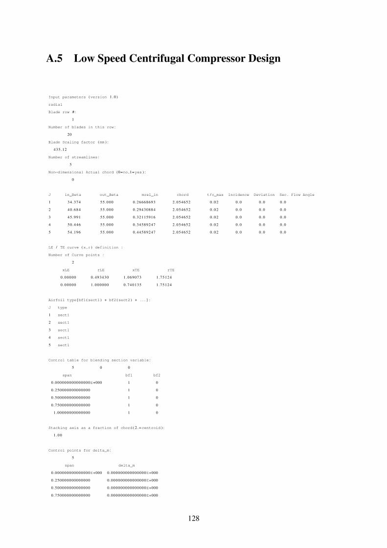
A.5 Low Speed Centrifugal Compressor Design

Input parameters (version 1 . 0 )

radial

Blade row # :

1

Number of blades in this row :

20

Blade Scaling factor (mm ) :

435 .12

Number of streamlines :

5

Non−dimensional Actual chord (0=no , 1=yes ) :

0

J in_Beta out_Beta mrel_in chord t /c_max Incidence Deviation Sec . Flow Angle

1 34 .374 55 .000 0 .26668693 2 .054652 0 . 0 2 0 . 0 0 . 0 0 . 0

2 40 .684 55 .000 0 .29430884 2 .054652 0 . 0 2 0 . 0 0 . 0 0 . 0

3 45 .991 55 .000 0 .32115916 2 .054652 0 . 0 2 0 . 0 0 . 0 0 . 0

4 50 .446 55 .000 0 .34589247 2 .054652 0 . 0 2 0 . 0 0 . 0 0 . 0

5 54 .196 55 .000 0 .44589247 2 .054652 0 . 0 2 0 . 0 0 . 0 0 . 0

LE / TE curve (x ,r ) definition :

Number of Curve points :

2

xLE rLE xTE rTE

0 .00000 0 .493430 1 .069073 1 .75124

0 .00000 1 .000000 0 .740135 1 .75124

Airfoil type{bf1 (sect1 ) + bf2 (sect2 ) + . . . } :

J type

1 sect1

2 sect1

3 sect1

4 sect1

5 sect1

Control table for blending section variable :

5 0 0

span bf1 bf2

0.000000000000000E+000 1 0

0.250000000000000 1 0

0.500000000000000 1 0

0.750000000000000 1 0

1.00000000000000 1 0

Stacking axis as a fraction of chord ( 2 . =centroid ) :

1 . 0 0

Control points for delta_m :

5

span delta_m

0.000000000000000E+000 0.000000000000000E+000

0.250000000000000 0.000000000000000E+000

0.500000000000000 0.000000000000000E+000

0.750000000000000 0.000000000000000E+000

128

1.00000000000000 0.000000000000000E+000

Control points for delta_theta :

5

span delta_theta

0.000000000000000E+000 0.0000000000000E+000

0.350000000000000 0.0000000000000E+000

0.500000000000000 0.0000000000000E+000

0.800000000000000 0.0000000000000E+000

1.00000000000000 0.0000000000000E+000

Control points for in_beta* :

5

span in_beta*

0.000000000000000E+000 0.000000000000000E+000

0.250000000000000 0.000000000000000E+000

0.500000000000000 0.000000000000000E+000

0.750000000000000 0.000000000000000E+000

1.00000000000000 0.000000000000000E+000

Control points for out_beta* :

5

span out_beta*

0.000000000000000E+000 0.000000000000000E+000

0.250000000000000 0.000000000000000E+000

0.500000000000000 0.000000000000000E+000

0.750000000000000 0.000000000000000E+000

1.00000000000000 0.000000000000000E+000

Control points for chord :

5

span chord

0.000000000000000E+000 0.000000000000000E+000

0.250000000000000 0.000000000000000E+000

0.500000000000000 0.000000000000000E+000

0.750000000000000 0.000000000000000E+000

1.00000000000000 0.000000000000000E+000

Control points for tm /c :

5

span tm /c

0.000000000000000E+000 0.000000000000000E+000

0.250000000000000 0.000000000000000E+000

0.500000000000000 0.000000000000000E+000

0.750000000000000 0.000000000000000E+000

1.00000000000000 0.000000000000000E+000

Hub offset

0.000000000000000E+000

Tip offset

0.000000000000000E+000

Streamline Data

x_s r_s

−0.384306398 0 .351355028

−0.116751701 0 .451820188

−0.029189649 0 .483692774

−0.01684271 0.487299596

0 .00000 0.493429629

0.042094824 0 .508785852

129

0.084125529 0 .52431743

0 .12603121 0 .540182938

0.167753493 0 .556524177

0.209238371 0 .573458586

0.250433673 0 .591087976

0.291289529 0 .609489336

0.331756527 0 .628728397

0.371790541 0 .648850892

0.411350432 0 .669895891

0.450392535 0 .691887295

0.488874334 0 .714840504

0.526755148 0 .738774361

0.563992002 0 .76369806

0.600538472 0 .789624701

0 .63634078 0 .816567154

0.671343078 0 .844543574

0 .70547688 0 .87357005

0.738667264 0 .903675308

0 .77082414 0 .934881182

0.801845698 0 .967213872

0.831618174 1 .000698428

0.860019765 1 .035355304

0.886916713 1 .071196222

0.912169516 1 .10820854

0.935655222 1 .146370886

0.957251563 1 .18563155

0.976862475 1 .225919057

0.994426825 1 .267145385

1.009916805 1 .309191258

1.023349651 1 .351939925

1.034776154 1 .395267053

1.044285255 1 .439055663

1.051993703 1 .483188316

1 .058041 1.527586413

1 .06257745 1 .572159174

1.065766685 1 .616857189

1.067781991 1 .661583701

1.068807685 1 .706330897

1.069073129 1 .747738555

1.069073129 1 .751241037

1.069073129 1 .766420757

1 .06524499 1 .780430686

1.061462125 1 .794440614

1.057749586 1 .808450542

1.049903935 1 .838803089

1.042618818 1 .867992738

1.028678985 1 .926365141

1.003180962 2 .043116841

0 0

−0.34076703 0.513516271

−0.122588596 0 .588865141

−0.039404647 0 .612769581

−0.02576634 0.615474697

−0.008756205 0 .620072221

0.027193016 0 .631589389

0.063094491 0 .643238072

0.102119588 0 .655188684

0.140979442 0 .667648292

0.179641995 0 .680742784

0.218062891 0 .694572819

130

0 .25619783 0 .70921671

0.294001712 0 .724739842

0 .33143041 0 .741190131

0.368441177 0 .758609234

0.404988107 0 .777024729

0.441024487 0 .796456897

0 .4765047 0.816926825

0.511379677 0 .838446291

0.545598341 0 .861027705

0.579102489 0 .884682386

0.611833115 0 .90942378

0.643720583 0 .935259986

0.674691752 0 .962207035

0.704662622 0 .990274694

0.733541322 1 .019473364

0.761228282 1 .049811087

0.787619277 1 .081289874

0.812602788 1 .113903923

0.836065166 1 .147628585

0.857906555 1 .182431168

0.878030141 1 .218256286

0.896360946 1 .255032577

0 .91285157 1 .292675699

0.927481729 1 .331080219

0.940267283 1 .370141053

0.951250862 1 .40974892

0.960504344 1 .449799538

0.968122874 1 .490191901

0.974220273 1 .530853385

0.978919608 1 .571702461

0 .98235527 1 .612690809

0.984670895 1 .653738337

0.986020351 1 .69482976

0.986594388 1 .733433018

0.986788932 1 .74363032

0.986838688 1 .762624448

0.983967584 1 .77761244

0.981130435 1 .792600777

0.978346031 1 .811660576

0.972461792 1 .843181191

0.966997955 1 .873829633

0 .95654308 1 .935121346

0.937419562 2 .057709942

0 0

−0.297227661 0 .675677514

−0.128425492 0 .725910094

−0.049619645 0 .741846387

−0.034689971 0 .743649798

−0.01751241 0.746714814

0.012291207 0 .754392926

0.042063454 0 .762158715

0.078207966 0 .770194429

0.114205392 0 .778772408

0 .15004562 0 .788026981

0.185692108 0 .798057662

0.221106132 0 .808944084

0.256246897 0 .820751287

0.291070279 0 .833529371

0.325531922 0 .847322578

0.359583678 0 .862162162

131

0.393174641 0 .87807329

0.426254252 0 .895079288

0.458767352 0 .913194521

0.490658209 0 .932430709

0.521864198 0 .952797619

0.552323152 0 .974303985

0.581964286 0 .996949922

0.610716239 1 .020738762

0.638501103 1 .045668206

0.665236946 1 .071732855

0.690838389 1 .098923745

0 .71521879 1 .127224444

0.738288863 1 .156611624

0.759960815 1 .18704863

0.780157887 1 .218491451

0.798808719 1 .250881021

0.815859418 1 .284146098

0.831276315 1 .318206012

0.845046654 1 .352969181

0.857184915 1 .388342181

0 .86772557 1 .424230787

0.876723433 1 .460543413

0.884252045 1 .497195486

0.890399545 1 .534120358

0.895261767 1 .571245748

0.898943855 1 .60852443

0 .9015598 1.645892972

0.903233016 1 .683328622

0.904115646 1 .719127482

0.904504734 1 .736019604

0.904604247 1 .758828139

0.902690177 1 .774794195

0.900798745 1 .79076094

0.898942476 1 .81487061

0 .89501965 1 .847559294

0.891377091 1 .879666529

0.884407175 1 .943877551

0.871658163 2 .072303043

0 0

−0.253688293 0 .837838757

−0.134262387 0 .862955047

−0.059834643 0 .870923194

−0.043613601 0 .871824899

−0.026268616 0 .873357407

−0.002610602 0 .877196463

0.021032416 0 .881079357

0.054296344 0 .885200175

0.087431341 0 .889896523

0.120449244 0 .895311179

0.153321325 0 .901542506

0.186014433 0 .908671458

0.218492083 0 .916762732

0.250710149 0 .925868611

0.282622667 0 .936035921

0.314179249 0 .947299596

0.345324795 0 .959689683

0.376003804 0 .973231752

0.406155026 0 .987942751

0.435718078 1 .003833713

0.464625908 1 .020912852

132

0.492813189 1 .039184191

0.520207989 1 .058639858

0.546740727 1 .079270489

0.572339584 1 .101061719

0 .59693257 1 .123992347

0.620448497 1 .148036404

0.642818303 1 .173159014

0.663974938 1 .199319326

0.683856465 1 .226468675

0 .70240922 1 .254551733

0.719587298 1 .283505757

0 .73535789 1 .313259618

0.749701059 1 .343736326

0.762611578 1 .374858143

0.774102546 1 .40654331

0.784200278 1 .438712654

0.792942522 1 .471287289

0.800381217 1 .504199072

0.806578817 1 .53738733

0.811603925 1 .570789035

0.815532439 1 .604358051

0.818448704 1 .638047608

0.820445682 1 .671827484

0.821636905 1 .704821946

0.822220537 1 .728408887

0.822369806 1 .75503183

0.821412771 1 .771975949

0.820467055 1 .788921102

0 .81953892 1 .818080644

0.817577507 1 .851937397

0.815756228 1 .885503424

0 .81227127 1 .952633756

0.805896764 2 .086896144

0 0

−0.210148924 1 .00000

−0.140099283 1 .00000

−0.070049641 1 .00000

−0.052537231 1 .00000

−0.035024821 1 .00000

−0.01751241 1 .00000

1 .37893E−06 1 .00000

0.030384721 1 .00020592

0 .06065729 1 .001020638

0.090852868 1 .002595376

0.120950542 1 .005027349

0.150922734 1 .008398833

0.180737268 1 .012774177

0.210350018 1 .018207851

0.239713412 1 .024749265

0.268774821 1 .032437029

0.297474949 1 .041306076

0.325753355 1 .051384216

0.353542701 1 .062690982

0.380777946 1 .075236716

0.407387617 1 .089028084

0.433303227 1 .104064396

0.458451691 1 .120329794

0.482765214 1 .137802215

0.506178066 1 .156455231

0.528628195 1 .176251839

133

0.550058605 1 .197149062

0.570417816 1 .219093583

0.589661013 1 .242027027

0.607752114 1 .26588872

0.624660553 1 .290612015

0.640365876 1 .316130493

0.654856361 1 .342373138

0.668125804 1 .369266639

0.680176503 1 .396747104

0.691020178 1 .424744438

0.700674986 1 .453194521

0.709161611 1 .482031164

0.716510388 1 .511202657

0 .72275809 1 .540654302

0.727946084 1 .570332322

0.732121024 1 .600191671

0.735337608 1 .630202243

0.737658347 1 .660326347

0.739158163 1 .690516409

0.739936339 1 .720798171

0.740135365 1 .751235521

0.740135365 1 .769157704

0.740135365 1 .787081265

0.740135365 1 .821290678

0.740135365 1 .856315499

0.740135365 1 .89134032

0.740135365 1 .961389961

0.740135365 2 .101489244

0 0

134