arX

iv:c

ond-

mat

/070

3375

v3 [

cond

-mat

.sta

t-m

ech]

16

Aug

200

7

Weakly coupled, antiparallel, totally asymmetric simple exclusion processes

Robert Juhasz∗

Research Institute for Solid State Physics and Optics, H-1525 Budapest, P.O.Box 49, Hungary

(Dated: August 12, 2013)

We study a system composed of two parallel totally asymmetric simple exclusion processes withopen boundaries, where the particles move in the two lanes in opposite directions and are allowed tojump to the other lane with rates inversely proportional to the length of the system. Stationary den-sity profiles are determined and the phase diagram of the model is constructed in the hydrodynamiclimit, by solving the differential equations describing the steady state of the system, analyticallyfor vanishing total current and numerically for nonzero total current. The system possesses phaseswith a localized shock in the density profile in one of the lanes, similarly to exclusion processes en-dowed with nonconserving kinetics in the bulk. Besides, the system undergoes a discontinuous phasetransition, where coherently moving delocalized shocks emerge in both lanes and the fluctuation ofthe global density is described by an unbiased random walk. This phenomenon is analogous to thephase coexistence observed at the coexistence line of the totally asymmetric simple exclusion pro-cess, however, as a consequence of the interaction between lanes, the density profiles are deformedand in the case of asymmetric lane change, the motion of the shocks is confined to a limited domain.

I. INTRODUCTION

The investigation of interacting stochastic driven diffu-sive systems plays an important role in the understand-ing of nonequilibrium steady states [1, 2]. As opposedto equilibrium statistical mechanics, phase transitionsmay occur in these systems even in one spatial dimen-sion [3]. The paradigmatic model of driven lattice gasesis the one-dimensional totally asymmetric simple exclu-sion process (TASEP) [4, 5], which exhibits boundaryinduced phase transitions [6] and the steady state ofwhich is exactly known [7, 8]. Beside theoretical interest,this model and its numerous variants have found a widerange of applications, such as the description of vehiculartraffic [9] or modeling of transport processes in biologi-cal systems [10]. Inspired by the traffic of cytoskeletalmotors [11], such models were introduced where a to-tally asymmetric exclusion process is coupled to a finitecompartment where the motion of particles is diffusive[12, 13, 14]. Recently, the attention has turned to exclu-sion processes endowed with various types of reactionswhich violate the conservation of particles in the bulk[15, 16, 17, 18, 19, 20, 21, 22, 23, 24, 25, 26, 27, 28].The simplest one among these models is the TASEP with“Langmuir kinetics”, where particles are created and an-nihilated also at the bulk sites of the system [16]—a pro-cess, which may serve as a simplified model for the co-operative motion of molecular motors along a filamentfrom which motors can detach and attach to it again. Forthese types of systems, the time scale of nonconservingprocesses compared to that of directed motion and theprocesses at the boundaries is crucial. If the nonconserv-ing reactions occur with rates of larger order than theinverse of the system size L, then in the large L limit,they dominate the stationary state. On the contrary,

∗Electronic address: juhasz@szfki.hu

when they are of smaller order than O(1/L), they areirrelevant and the stationary state is identical to that ofthe underlying driven diffusive system. However, in themarginal case when the rates of nonconserving processesare of order O(1/L), the interplay between them and theboundary processes may result in intriguing phenomena,such as ergodicity breaking [19, 24] or the appearanceof a localized shock in the density profile [16], which isin contrast to the delocalized shock dynamics at the co-existence line of the TASEP [8, 29]. The formation ofdomain walls can be observed also experimentally in thetransport of kinesin motors in accordance with theoreti-cal predictions [30, 31, 32].

Other systems which have an intermediate complexitycompared to exclusion processes with bulk reactions andthose coupled to a compartment are the two-channel ormultichannel systems. In these models, particles are ei-ther conserved by the dynamics in each lane and interac-tion is realized by the dependence of the hop rates on theconfiguration of the parallel lanes [33, 34, 35, 36, 37, 38],or particles can jump between lanes [39, 40, 41, 42]. Westudy in this work a two-lane exclusion process whereparticles move in the two lanes in opposite directions.Particles are allowed to change lanes and we restrict our-selves to the case of weak lane change rates, i.e. theyare inversely proportional to the system size. This meansthat the probability that a marked particle changes lanesduring the time it resides in the system is O(1). If par-ticles in one of the lanes are regarded as holes, and viceversa, this model can also be interpreted as a two-channeldriven system where particles move in the same directionin the channels and are created and annihilated in pairs.In the hydrodynamic limit of the model, we shall con-struct the steady-state phase diagram by means of ana-lyzing the differential equations describing the model onthe macroscopic scale. At the coexistence line, where co-herently moving delocalized shocks develop in both lanes,which is reminiscent of the delocalized shock dynamics atthe coexistence line of the TASEP, the density profiles are

2

studied in the framework of a phenomenological domainwall picture based on the hydrodynamic description. Re-cently, a two-lane exclusion process has been investigatedwith weak, symmetric lane change, where particles movein the lanes in the same direction [42]. In this model, theformation of delocalized shocks in both lanes has beenfound, as well. In our model, even the case of asymmetriclane change can be treated analytically in the hydrody-namic limit if the total current is zero, which holds alsoat the coexistence line.

The paper is organized as follows. In Sec. II, themodel is introduced and the hydrodynamic descriptionis discussed. In Sec. III, the case of symmetric lanechange is investigated, while Sec. IV is devoted to theasymmetric case. The results are discussed in Sec. V andsome of the calculations are presented in two Appendixes.

II. DESCRIPTION OF THE MODEL

The model we focus on consists of two parallel one-dimensional lattices with L sites, denoted by A and B,the sites of which are either empty or occupied by a parti-cle. The state of the system is specified by the set of occu-

pation numbers nA,Bi which are zero (one) for empty (oc-

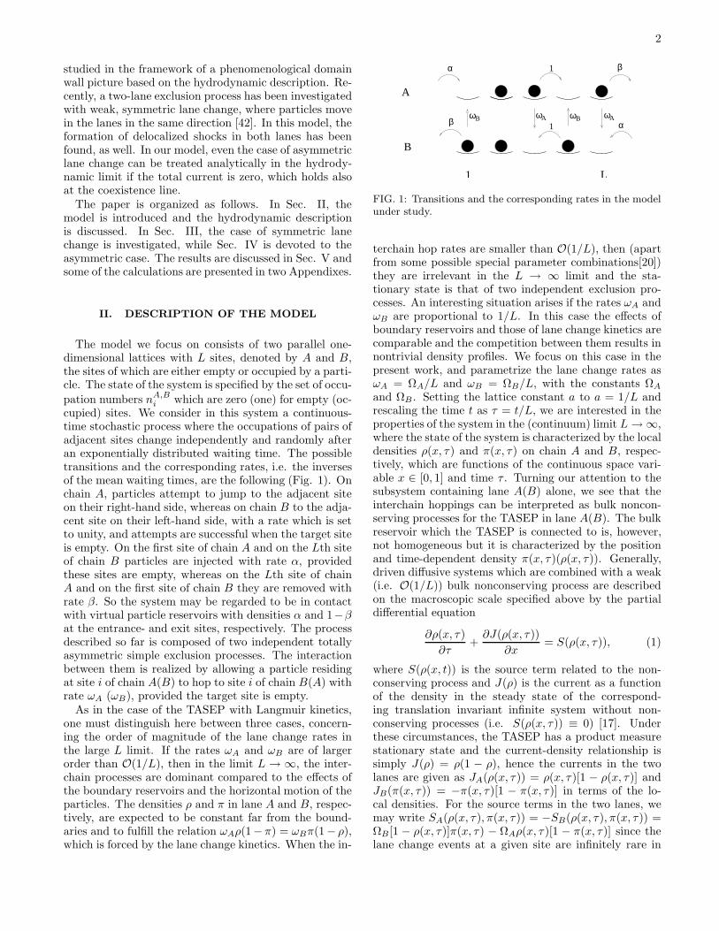
cupied) sites. We consider in this system a continuous-time stochastic process where the occupations of pairs ofadjacent sites change independently and randomly afteran exponentially distributed waiting time. The possibletransitions and the corresponding rates, i.e. the inversesof the mean waiting times, are the following (Fig. 1). Onchain A, particles attempt to jump to the adjacent siteon their right-hand side, whereas on chain B to the adja-cent site on their left-hand side, with a rate which is setto unity, and attempts are successful when the target siteis empty. On the first site of chain A and on the Lth siteof chain B particles are injected with rate α, providedthese sites are empty, whereas on the Lth site of chainA and on the first site of chain B they are removed withrate β. So the system may be regarded to be in contactwith virtual particle reservoirs with densities α and 1−βat the entrance- and exit sites, respectively. The processdescribed so far is composed of two independent totallyasymmetric simple exclusion processes. The interactionbetween them is realized by allowing a particle residingat site i of chain A(B) to hop to site i of chain B(A) withrate ωA (ωB), provided the target site is empty.

As in the case of the TASEP with Langmuir kinetics,one must distinguish here between three cases, concern-ing the order of magnitude of the lane change rates inthe large L limit. If the rates ωA and ωB are of largerorder than O(1/L), then in the limit L → ∞, the inter-chain processes are dominant compared to the effects ofthe boundary reservoirs and the horizontal motion of theparticles. The densities ρ and π in lane A and B, respec-tively, are expected to be constant far from the bound-aries and to fulfill the relation ωAρ(1− π) = ωBπ(1− ρ),which is forced by the lane change kinetics. When the in-

ωA ωBωB ωAβ 1

1α

A

B

1 L

β

α

FIG. 1: Transitions and the corresponding rates in the modelunder study.

terchain hop rates are smaller than O(1/L), then (apartfrom some possible special parameter combinations[20])they are irrelevant in the L → ∞ limit and the sta-tionary state is that of two independent exclusion pro-cesses. An interesting situation arises if the rates ωA andωB are proportional to 1/L. In this case the effects ofboundary reservoirs and those of lane change kinetics arecomparable and the competition between them results innontrivial density profiles. We focus on this case in thepresent work, and parametrize the lane change rates asωA = ΩA/L and ωB = ΩB/L, with the constants ΩA

and ΩB. Setting the lattice constant a to a = 1/L andrescaling the time t as τ = t/L, we are interested in theproperties of the system in the (continuum) limit L → ∞,where the state of the system is characterized by the localdensities ρ(x, τ) and π(x, τ) on chain A and B, respec-tively, which are functions of the continuous space vari-able x ∈ [0, 1] and time τ . Turning our attention to thesubsystem containing lane A(B) alone, we see that theinterchain hoppings can be interpreted as bulk noncon-serving processes for the TASEP in lane A(B). The bulkreservoir which the TASEP is connected to is, however,not homogeneous but it is characterized by the positionand time-dependent density π(x, τ)(ρ(x, τ)). Generally,driven diffusive systems which are combined with a weak(i.e. O(1/L)) bulk nonconserving process are describedon the macroscopic scale specified above by the partialdifferential equation

∂ρ(x, τ)

∂τ+

∂J(ρ(x, τ))

∂x= S(ρ(x, τ)), (1)

where S(ρ(x, t)) is the source term related to the non-conserving process and J(ρ) is the current as a functionof the density in the steady state of the correspond-ing translation invariant infinite system without non-conserving processes (i.e. S(ρ(x, τ)) ≡ 0) [17]. Underthese circumstances, the TASEP has a product measurestationary state and the current-density relationship issimply J(ρ) = ρ(1 − ρ), hence the currents in the twolanes are given as JA(ρ(x, τ)) = ρ(x, τ)[1 − ρ(x, τ)] andJB(π(x, τ)) = −π(x, τ)[1 − π(x, τ)] in terms of the lo-cal densities. For the source terms in the two lanes, wemay write SA(ρ(x, τ), π(x, τ)) = −SB(ρ(x, τ), π(x, τ)) =ΩB[1 − ρ(x, τ)]π(x, τ) − ΩAρ(x, τ)[1 − π(x, τ)] since thelane change events at a given site are infinitely rare in

3

the limit L → ∞. Setting these expressions into eq. (1)we obtain that in the steady state, where ∂τρ(x, τ) =∂τπ(x, τ) = 0, the density profiles ρ(x) and π(x) satisfythe coupled differential equations

(2ρ − 1)∂xρ + ΩB(1 − ρ)π − ΩAρ(1 − π) = 0,

(2π − 1)∂xπ + ΩB(1 − ρ)π − ΩAρ(1 − π) = 0. (2)

We mention that one arrives at the same differentialequations when in the master equation of the process theexpectation values of pairs of occupation numbers 〈ninj〉are replaced by the products 〈ni〉〈nj〉, and afterwards itis turned to a continuum description with retaining onlythe first derivatives of the densities and neglecting thehigher derivatives which are at most of the order O(1/L)almost everywhere.

For the stationary density profiles the boundary con-ditions ρ(0) = π(1) = α and ρ(1) = π(0) = 1 − β areimposed. In fact, we shall keep these boundary condi-tions only for α, β ≤ 1/2; otherwise, we modify themfor practical purposes at the level of the hydrodynamicdescription. The reason for this is the following. In thedomain α, β > 1/2 of the TASEP, the so-called maximumcurrent phase, the current is limited by the maximal car-rying capacity in the bulk, J = 1/4, which is realized atthe bulk density ρ = 1/2 [7, 8]. In this phase, boundarylayers form in the stationary density profile at both ends,where the density drops to the bulk value ρ = 1/2. Sim-ilarly, in the case of the TASEP with Langmuir kinetics,if the entrance rate α exceeds the value 1/2, then in thedensity profile dictated by the reservoir at the entrancesite, a boundary layer develops, where the density dropsto 1/2. The width of the boundary layer is growing sub-linearly with L [20], such that in the hydrodynamic limit,it shrinks to x = 0 and limx→0 ρ(x) = 1/2 holds, inde-pendently of α, which influences only the shape of themicroscopic boundary layer. These considerations applyalso to the present model at both ends and for both lanes.Therefore, in order to simplify the treatment of the prob-lem at the level of the hydrodynamic description, we usethe effective boundary conditions

ρ(0) = π(1) = a, ρ(1) = π(0) = 1 − b, (3)

where a ≡ minα, 1/2 and b ≡ minβ, 1/2. However,we stress that, although, the profile propagating frome.g. the left-hand boundaryρl(x) is continuous at x =0 according to the effective boundary conditions (3) forα > 0, a boundary layer forms on the microscopic scale.

In addition to the boundary layers related to the maxi-mal carrying capacity in the bulk, the stationary densityprofiles may in general contain another type of bound-ary layer of finite width or a localized shock in the bulk,where the density has a finite variation within a regionthe width of which is growing sublinearly with L [16, 18].This leads to the appearance of discontinuities in ρ(x)and π(x) in the hydrodynamic limit, either in the bulk0 < x < 1 in the case of a shock or at x = 0, 1 in the caseof a boundary layer. This is in accordance with the fact

that, in general, there does not exist a continuous solu-tion to the two first order differential equations, whichfulfills all four boundary conditions. Apart from somespecial parameter combinations, there is one discontinu-ity in each lane, which is either in the bulk (a shock) or atx = 0, 1 (a boundary layer). The location of the disconti-nuity is determined by the requirement that the currentsin both lanes JA(ρ(x)) and JB(ρ(x)) must be continuousfunctions of x in the bulk 0 < x < 1 [17, 18]. This followsfrom that the width of the shock region is proportionalto

√L, thus the rate of a lane change event is vanishing

there in the limit L → ∞. This condition permits onlysuch a shock which separates complementary densities onits two sides, i.e. ρ and 1 − ρ in lane A or π and 1 − πin lane B. The position of the shock xs e.g. in lane A isthus given implicitly by the equation ρl(xs) = 1−ρr(xs),where ρl(x) and ρr(x) are the solutions on the two sidesof the shock. For the detailed rules on the stability ofthe discontinuity at x = 0, 1 see Ref. [17].

Subtracting the two differential equations yields theobvious result that the total current

J ≡ ρ(x)[1 − ρ(x)] − π(x)[1 − π(x)] (4)

is a (position independent) constant. This relation makesit possible to eliminate one of the functions, say, π(x)and to reduce the problem to the integration of a singledifferential equation

dρ

dx= ΩA

ρ − [ 12 ±√

(ρ − 12 )2 + J ][K(1 − ρ) + ρ]

2ρ − 1, (5)

where we have introduced the ratio of lane change ratesK ≡ ΩB/ΩA and the signs in front of the square root arerelated to the two solutions π+(x) > 1/2 and π−(x) <1/2 of the quadratic equation (4). Disregarding the sim-ple case K = 1, there are two difficulties about this equa-tion. First, the solution depends on the current J as a pa-rameter, which itself depends on the density profiles andis a priori not known. Fortunately, apart from two phasesin the phase diagram, ρ(x) and π(x) simultaneously fit tothe boundary conditions either at x = 0 or x = 1, con-sequently, the current is exclusively determined by theentrance- and exit rates as J = a(1 − a) − b(1 − b). Inthe remaining two phases, the functions ρ(x) and π(x)meet the boundary conditions at the opposite ends ofthe system. Here, one may solve eq. (5) iteratively un-til self-consistency is attained. Second, even in the casewhen J is known, eq. (5) cannot be analytically inte-grated in general, except for the case when the current iszero. This is realized in three cases, two of which are re-lated to the symmetries of the system. We discuss thesepossibilities in the rest of the section.

As the two entrance- and exit rates were chosen to beidentical, the obvious relation holds when the rates ΩA

and ΩB are interchanged:

ρ(x; α, β, ΩA, ΩB) = π(1 − x; α, β, ΩB , ΩA), (6)

4

where the dependence of the profiles on the four parame-ters α,β,ΩA and ΩB is explicitly indicated. This relation,together with eq. (4) implies that the current changessign if ΩA and ΩB are interchanged. Thus ΩA = ΩB

implies J = 0, that holds apparently since none of thechains is singled out in this case.

As a consequence of the particle-hole symmetry of themodel, we have the relation

ρ(x; α, β, ΩA, ΩB) = 1 − π(x; β, α, ΩA, ΩB). (7)

Using eq. (4), it follows that the current changes signwhen α and β are interchanged, so it must be zero forα = β. Alternatively, this can be seen by interchangingparticles and holes in one of the chains, which results in atwo-channel system where particles move in the channelsin the same direction and particles are created and anni-hilated in pairs at neighboring sites of the two chains withrates ΩA and ΩB, respectively. Particles are injected andremoved in the channels with the same rate, hence thechannels are equivalent. Since the currents of particlesand holes are equal, the total current must be zero.

The third parameter regime where the current is zerois the domain α, β ≥ 1/2. Here, as aforesaid, the densityprofiles and the current are independent of α and β in thehydrodynamic limit. Since the current is zero for α = βit follows that J = 0 in the whole domain α, β ≥ 1/2.

III. SYMMETRIC LANE CHANGE

We start the investigation of the model with the simplecase of equal lane change rates (ΩA = ΩB ≡ Ω), wherethe solutions to the hydrodynamic equations are analyt-ically found and some general features of the model canbe understood. Since the total current is zero, eitherρ(x) = π(x) or ρ(x) = 1 − π(x) must hold. Substitutingthe former relation into eq. (2) yields

ρe(x) = πe(x) = const, (8)

whereas the latter gives

ρc(x) = 1 − πc(x) = Ωx + const. (9)

Thus, the profiles are piecewise linear and consist of con-stant segments with equal densities in the two lanes andsegments of slope Ω (−Ω) in lane A(B) with comple-mentary densities. Switching off the interchain particleexchange (Ω = 0), we get two identical TASEPs, whichhave, apart from the coexistence line α = β < 1/2, con-stant density profiles in the bulk. In the high-densityphase (β < minα, 1/2), the density, being 1−β, is con-trolled by the exit rate and the profile is discontinuous atx = 0. In the low-density phase (α < minβ, 1/2), thedensity is α and a discontinuity appears at x = 1 [7, 8].In the maximum current phase (α, β > 1/2), as we havealready mentioned, the bulk density is 1/2 and boundarylayers appear at both ends. On the other hand, the effect

of symmetric lane change processes is to diminish the dif-ference between the local densities in the two lanes. Sincethe densities are already equal without the interaction,this situation is obviously not altered when switching onthe vertical hopping processes. Consequently, the densityprofiles in the bulk are identical to that of the TASEP inthese phases.

This is, however not the case at the coexistence lineα = β < 1/2. In the TASEP, a sharp domain wallemerges here in the density profile, which separates alow- and a high-density phase with constant densities farfrom the domain wall α and 1 − α, respectively. Thestochastic motion of the domain wall is described by anunbiased random walk with reflective boundaries [8, 29],such that the average stationary density profile connectslinearly the boundary densities α and 1 − α. Return-ing to our model, we consider first the closed system, i.e.α = β = 0. The profiles which fulfill the requirementabout the continuity of the currents are depicted in Fig.2 for various global particle densities ≡ limL→∞

N2L ,

where N is the number of particles in the system. Here,the density profiles consist of three segments in general.In the middle part of the system an equal-density seg-ment is found (Fig. 2a,b,d). This region is connectedwith the boundaries by complementary-density segmentson its left-hand side and on its right-hand side, whichare continuous at x = 0 and x = 1, respectively. In bothlanes, the density profile is continuous at one end of theequal-density segment and a shock is located at the otherone, such that the two shocks are at opposite ends. Thedensity in the equal-density region (and at the same timethe location of the shocks) depend on the global particledensity. At = 1/2, the equal-density segment is lackingif Ω < 1 (Fig. 2c) and the profiles are linear if Ω = 1.

0

1

ρ(x)

, π(x

)

a)

0

1

ρ(x)

, π(x

)

a)

0

1

ρ(x)

, π(x

)

a)

0

1

ρ(x)

, π(x

)

a)

0

1

ρ(x)

, π(x

)

a)

0

1

ρ(x)

, π(x

)

a)

0

1

ρ(x)

, π(x

)

a)

0

1

ρ(x)

, π(x

)

a)

0

1

ρ(x)

, π(x

)

a)

0

1

ρ(x)

, π(x

)

a) b)b)b)b)b)b)b)b)b)b)

0

1

0 1

ρ(x)

, π(x

)

x

c)

0

1

0 1

ρ(x)

, π(x

)

x

c)

0

1

0 1

ρ(x)

, π(x

)

x

c)

0

1

0 1

ρ(x)

, π(x

)

x

c)

0

1

0 1

ρ(x)

, π(x

)

x

c)

0

1

0 1

ρ(x)

, π(x

)

x

c)

0

1

0 1

ρ(x)

, π(x

)

x

c)

0

1

0 1

ρ(x)

, π(x

)

x

c)

0 1x

d)

0 1x

d)

0 1x

d)

0 1x

d)

0 1x

d)

0 1x

d)

0 1x

d)

0 1x

d)

0 1x

d)

0 1x

d)

FIG. 2: Density profiles of the closed system (α = β = 0)with Ω = 0.5 for different global densities: (a) = 0.26, (b) = 0.44, (c) = 0.5 and (d) = 0.74. The thin solid anddashed lines represent the flow field of the differential equation(5) corresponding to the complementary-density and equal-density solutions, respectively. The thick solid and dashedlines are the density profiles ρ(x) and π(x), respectively.

5

If particles are allowed to enter and exit from the sys-tem at the boundaries, i.e. 0 < α = β < 1/2, the totalnumber of particles is no longer conserved. Nevertheless,we expect that the stationary density profiles averagedover configurations with a fixed global density , ρ(x)and π(x), can still be constructed from the solutions (8)and (9) of the hydrodynamic equations. These profilesare similar to those of the closed system and the only dif-ference is that the complementary-density segments fit tothe altered boundary conditions ρ(0) = π(1) = α andρ(1) = π(0) = 1−α. This is indeed the case in the limitα → 0. Here, the injections and removals of particles atthe boundary sites, which modify the global density, areinfinitely rare, such that the system has always enoughtime to relax, i.e. to adjust the density profiles to theslightly altered global density. As long as the shocksare not in the vicinity of the boundaries, the densitiesat the boundary sites are independent from the globaldensity, which influences only the position of the equaldensity segment. Therefore, the stochastic variation ofthe global density (t) is described by a homogeneous,symmetric random walk in the interval [0, 1] with reflec-tive boundary conditions. For finite α, we can give only aheuristic argument why we expect that the fluctuationsof the global density are quasistationary in the abovesense. In the stationary state, the center of the mass of asmall instantaneous local perturbation propagates witha velocity v(x) = 1 − 2ρ(x) [29, 43], which changes signat ρ = 1/2. In the complementary-density segments,the perturbations in the density, which come from thefluctuations of the boundary reservoirs, are thus driventoward the equal-density segment with a finite velocity.The characteristic traveling time of the perturbation, aswell as the time scale related to the lane change processesin a finite system of size L is O(L). The relaxation time ofthe perturbation is thus expected to be O(L). However,the random walk dynamics of the global density impliesthat the time scale of a finite change in the global den-sity is O(L2), which is large compared to the relaxationtime, thus the density profile has enough time to followthe instantaneous global density. The fluctuating globaldensity (t) is thus expected to be a symmetric randomwalk with reflective boundaries at α and 1 − α. In thestationary state, the global density is therefore homoge-neously distributed in the interval [α, 1 − α].

On the other hand, one can easily calculate that if theposition of the shock in lane A is xs, the global density ofparticles in the system is (xs) = (1−xs)[∆(xs)+Ω]+αfor xs ≥ 1/2, where we have introduced the (positiondependent) height of the shock: ∆(xs) = 2Ω(xs − 1) +1− 2α. Note that, as opposed to the single lane TASEP,this relation is no longer linear, therefore the probabilitydistribution of the position of the shock is not uniformin the steady state.

With these prerequisites, the steady-state density pro-file in lane A can be easily calculated by averaging ρ(x)over the steady-state distribution of the global density:

ρ(x) = 11−2α

∫ 1−α

α ρ(x)d. Skipping the details of the

0

1

⟨niA

⟩

a)

Ω=0.4

L=64L=128L=256

0

1

⟨niA

⟩

a)

Ω=0.4

continuum

0

1

⟨niA

⟩

a)

Ω=0.4

0

1

⟨niA

⟩

a)

Ω=0.4

0

1

⟨niA

⟩

a)

Ω=0.4

0

1

⟨niA

⟩

b)

Ω=0.8

L=64L=128L=256

0

1

⟨niA

⟩

b)

Ω=0.8

continuum

0

1

⟨niA

⟩

b)

Ω=0.8

0

1

0 1

⟨niA

⟩

(i-0.5)/L

c)

Ω=1.2

L=64L=128L=256

0

1

0 1

⟨niA

⟩

(i-0.5)/L

c)

Ω=1.2

continuum

0

1

0 1

⟨niA

⟩

(i-0.5)/L

c)

Ω=1.2

0

1

0 1

⟨niA

⟩

(i-0.5)/L

c)

Ω=1.2

0

1

0 1

⟨niA

⟩

(i-0.5)/L

c)

Ω=1.2

0

1

0 1

⟨niA

⟩

(i-0.5)/L

c)

Ω=1.2

FIG. 3: Density profiles in lane A at the coexistence line atα = β = 0.1, obtained by numerical simulation for differentsystem sizes and for different values of Ω: a) Ω = 0.4, b)Ω = 0.8, and c) Ω = 1.2. In the case Ω = 0.8, the height of theshock at xs = 1/2 is zero. The solid curves are the analyticalpredictions in the hydrodynamic limit. The thick solid linesrepresent the profile ρ(x) at global density = 1/2.

straightforward calculations, we shall give the profile ρ(x)in the interval 1

2 ≤ x ≤ 1, whereas for 0 ≤ x ≤ 12 , it is

obtained by the help of the relation ρ(x) = 1 − ρ(1− x),that follows from eq. (6) and (7). The density profile inlane B can be calculated by making use of eq. (7), whichimplies π(x) = 1 − ρ(x). The cases corresponding to thedifferent signs of ∆(1

2 ) must be treated separately. For

∆(12 ) ≥ 0, we obtain

ρ(x) =1

2+

(x − 12 )∆2(x)

1 − 2α∆(

1

2) ≥ 0, (10)

6

which is a third-degree polynomial of x. If ∆(12 ) > 0,

the second derivative of ρ(x) is discontinuous at x = 12 .

In the limit Ω → 0, the linear profile of the TASEP atthe coexistence line is recovered. If ∆(1

2 ) = 0, eq. (10)simplifies to

ρ(x) =1

2+ 4Ω(x − 1

2)3 ∆(

1

2) = 0, (11)

which is everywhere analytic. For ∆(12 ) < 0, the profile

is constant in the interval 12 ≤ x ≤ |∆(1

2 )|/(2Ω) + 12 ,

where ρ(x) = 1/2, while it is given by eq. (10) in theinterval |∆(1

2 )|/(2Ω) + 12 ≤ x ≤ 1. These curves, as well

as results of Monte Carlo simulations for finite systemsof size L = 64, 128 and 256 are shown in Fig 3. In the nu-merical simulations, after waiting a period of 106 MonteCarlo steps in order to reach the steady state, we havemeasured the local occupancies every 10 Monte Carlosteps during a period of 5 · 109 steps. For increasing L,the properly scaled profiles seem to tend to the analyticalcurves expected to be valid in the continuum limit.

IV. ASYMMETRIC LANE CHANGE

In this section, the stationary properties of the modelare investigated in the case K 6= 1. Due to the sym-metries of the system, we may restrict ourselves to theinvestigation of the part K < 1, β ≤ α of the parame-ter space, which is related to the remaining part througheqs. (6) and (7). Analyzing the solutions to the hydro-dynamic equation (5), one can construct the phase di-agram in the four-dimensional parameter space spannedby α, β, ΩA and ΩB . Two representative two-dimensionalcross sections of the parameter space at fixed lane changerates are shown in Fig. 4 and 5. As can be seen, thephase boundaries are symmetric to the diagonal, whichis a consequence of eq. (7). On the other hand, thephase diagrams are richer compared to that of the sym-metric model: Besides the phases where the profiles arecontinuous in the interior of the system, the asymmetryin the lane change kinetics leads to the appearance ofphases where one of the lanes contains a localized shockin the bulk. This is reminiscent of the shock phase of thesingle lane TASEP with Langmuir kinetics. As a new fea-ture, the position of the shock may vary discontinuouslywith the boundary rates here, when the so-called discon-tinuity line is crossed. The coexistence line, where coher-ently moving delocalized shocks emerge in both lanes, isstill present, however, it is shorter than in the symmetriccase and the shocks walk only a shrunken domain. Thesubsequent part of the section is devoted to the detailedanalysis of these findings.

A. Density profiles

We start the presentation of the results with the de-scription of the density profiles in the phases below the

0

ρ1

0.5

1

0 ρ1 0.5 1

α

β

L-H

H-H

S-H

L-S

L-L

0

ρ1

0.5

1

0 ρ1 0.5 1

α

β

L-H

H-H

S-H

L-S

L-L

0

ρ1

0.5

1

0 ρ1 0.5 1

α

β

L-H

H-H

S-H

L-S

L-L

0

ρ1

0.5

1

0 ρ1 0.5 1

α

β

L-H

H-H

S-H

L-S

L-L

0

ρ1

0.5

1

0 ρ1 0.5 1

α

β

L-H

H-H

S-H

L-S

L-L

0

ρ1

0.5

1

0 ρ1 0.5 1

α

β

L-H

H-H

S-H

L-S

L-L

FIG. 4: Phase diagram at ΩA = 2, ΩB = 0.4. Phase bound-aries are indicated by solid lines. Letters L,H and S refer tolow-density, high-density and localized shock phase, respec-tively; the first(second) letter refers to lane A(B). The thicksolid line indicates the coexistence line. At the dashed lines,the function J(α, β) is nonanalytic.

0

ρ1

0.5

1

0 ρ1 0.5 1

α

β

L-H

H-H

S-H

L-S

L-L

0

ρ1

0.5

1

0 ρ1 0.5 1

α

β

L-H

H-H

S-H

L-S

L-L

0

ρ1

0.5

1

0 ρ1 0.5 1

α

β

L-H

H-H

S-H

L-S

L-L

0

ρ1

0.5

1

0 ρ1 0.5 1

α

β

L-H

H-H

S-H

L-S

L-L

0

ρ1

0.5

1

0 ρ1 0.5 1

α

β

L-H

H-H

S-H

L-S

L-L

0

ρ1

0.5

1

0 ρ1 0.5 1

α

β

L-H

H-H

S-H

L-S

L-L

0

ρ1

0.5

1

0 ρ1 0.5 1

α

β

L-H

H-H

S-H

L-S

L-L

0

ρ1

0.5

1

0 ρ1 0.5 1

α

β

L-H

H-H

S-H

L-S

L-L

0

ρ1

0.5

1

0 ρ1 0.5 1

α

β

L-H

H-H

S-H

L-S

L-L

FIG. 5: Phase diagram at ΩA = 2, ΩB = 1. The dotted curvesare the discontinuity lines, which terminate at the points in-dicated by the full circles.

diagonal α = β of the two-dimensional phase diagrams.

If the exit rate is small enough, the densities in thebulk exceed the value 1/2 in both lanes (Fig. 6a). Bothprofiles are continuous in the bulk and at the exits, i.e.limx→1 ρ(x) = limx→0 π(x) = 1 − b, but they are dis-continuous at the entrances, i.e. limx→0 ρ(x) 6= a andlimx→1 π(x) 6= a, which signals the appearance of bound-ary layers on the microscopic scale. The profiles ρ(x)

7

and π(x), as well as the current, depend exclusively onβ, while α influences only the boundary layers at theentrances. This situation is observed also in the high-density phase of the TASEP with Langmuir kinetics[16, 18], therefore we call this phase H-H phase, refer-ring to the high density in both lanes.

0

1

0 1

b)

1-β1-β

α

0

1

0 1

b)

1-β1-β

α

0

1

0 1

b)

1-β1-β

α

0

1

0 1

b)

1-β1-β

α

0

1

0 1

b)

1-β1-β

α

0

1

0 1

b)

1-β1-β

α

0

1

0 1

ρ(x)

, π(x

)

x

c)

1-β

α

0

1

0 1

ρ(x)

, π(x

)

x

c)

1-β

α

0

1

0 1

ρ(x)

, π(x

)

x

c)

1-β

α

0

1

0 1

ρ(x)

, π(x

)

a)

1-β 1-β

0

1

0 1

ρ(x)

, π(x

)

a)

1-β 1-β

0

1

0 1

ρ(x)

, π(x

)

a)

1-β 1-β

0

1

0 1x

d)

1-αα

0

1

0 1x

d)

1-αα

FIG. 6: Density profiles in lane A (lower line) and lane B (up-per line) for the parameters ΩA = 2, ΩB = 0.4, α = 0.45 andfor various exit rates: a) β = 0.15, b) β = 0.25, c) β = 0.35and d) β = 0.45. The profiles in panels a)-c) were obtainedby numerically solving eq. (5), whereas those in panel d) arethe analytical curves in eq. (14). Results of numerical sim-ulations (dotted lines) obtained for system size L = 10000by averaging the occupancies in a period of 107 Monte Carlosteps in the steady state are hardly distinguishable from thesecurves.

In the phase denoted by S-H in the phase diagram, ρ(x)and π(x) are continuous at the exits, similarly to the H-H phase, however, the discontinuity in ρ(x) is no longerat x = 0 but it is shifted to the interior of the system(Fig. 6b). Thus limx→0 ρ(x) = a holds and a shock islocated in lane A at some xs (0 < xs < 1). Thereforethis phase is termed S-H phase, where the letter S refersto the shock in lane A and letter H refers to the highdensity (π(x) > 1/2) in lane B. The function π(x) isdiscontinuous at x = 1, i.e. limx→1 π(x) 6= a and it is notdifferentiable (although continuous) at xs. Since bothρ(x) and π(x) are continuous at x = 0, the total currentis given by

J = a(1 − a) − b(1 − b) (12)

in this phase. The profile ρ(x) at fixed α and β canbe computed by substituting the current calculated fromeq. (12) into the differential equation (5). Then, thesolutions propagating from the left-hand and the right-hand boundary, i.e. the solutions ρl(x) and ρr(x) fulfill-ing the boundary conditions ρl(0) = a and ρr(1) = 1− b,respectively, are calculated numerically. Finally, theposition of the shock xs is obtained from the relationρl(xs) = 1−ρr(xs), which is implied by the continuity of

the current in lane A. Once ρ(x) is at our disposal, π(x)can be calculated from eq. (4).

Apart from the discontinuity line to be discussed in thenext section, the position of the shock xs varies continu-ously with the boundary rates in the S-H phase. Fixing αand reducing β, xs is decreasing and at a certain value ofβ, β = βH(α), the shock reaches the left-hand boundaryat x = 0. At this point, the right-hand solution ρr(x)extends entirely to the left-hand boundary and a furtherincrease in β drives the system to the H-H phase. Thephase boundary βH(α) between the S-H and the H-Hphase is thus determined from the condition xs = 0 or,equivalently, ρr(1) = 1 − a. When β is increased alonga vertical path in the phase diagram at a fixed α, xs in-creases and for α < ρ1, where the constant ρ1 will bedetermined later, the path hits the coexistence line be-fore the shock would reach the right-hand boundary (seeSec. III. D). Increasing β along a path at some α > ρ1,the shock reaches the right-hand boundary at x = 1 for acertain value of β, β = βL(α) and the path leaves the S-H phase. At the phase boundary, the left-hand solutionρl(x) extends to the whole system and ρl(1) = b musthold.

Crossing the phase boundary βL(α), the L-H phase isentered, where letter L refers to the low density in laneA since here, ρ(x) < 1/2 and π(x) > 1/2 hold in the bulk(Fig. 6c). In this phase, ρ(x) and π(x) are discontinuousat x = 1, whereas they are continuous at x = 0 hence thecurrent is given by eq. (12). In the part of the L-H phasewhere the current is zero, i.e. if α = β or α, β ≥ 1/2, theprofiles can be calculated analytically. The equal-densitysolutions of eq. (5) are

ln[ρe(x)(1 − ρe(x))] = ΩA(K − 1)x + const,

πe(x) = ρe(x), (13)

whereas the complementary-density solutions read as

ρ1

ρ2ln |ρc(x) − ρ1| −

ρ2

ρ1ln |ρc(x) − ρ2| = 2ΩA

√Kx + const,

πc(x) = 1 − ρc(x), (14)

where the constants ρ1 ≡ 1/(1+K−1/2) and ρ2 ≡ 1/(1−K−1/2) are the roots of the equation SA(ρ, 1 − ρ) = 0.There is, furthermore, a special complementary-densitysolution with constant densities:

ρc(x) = ρ1,

πc(x) = 1 − ρ1. (15)

In the part of the L-H phase where J = 0, the profilesare given by the complementary-density solution whichfulfills the boundary conditions ρc(0) = a and πc(0) =1 − a (Fig. 6d).

B. Phase boundaries and the discontinuity line

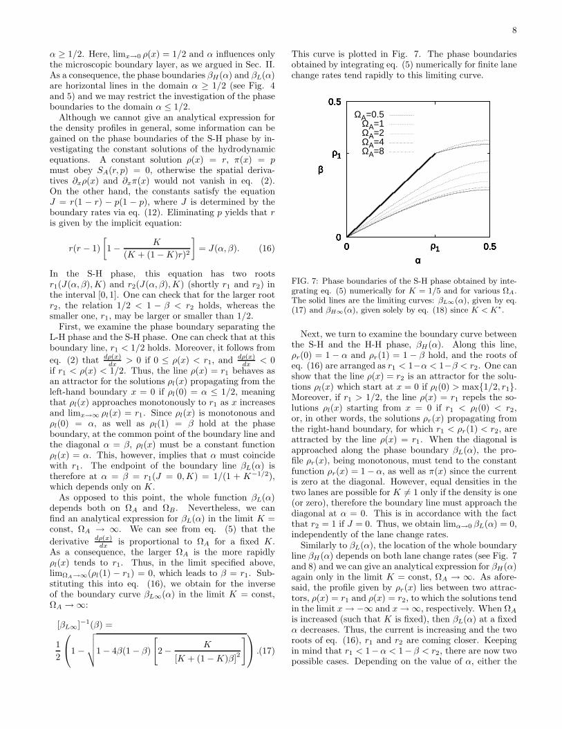
In the S-H phase (and the L-H phase), the profiles ρ(x)and π(x), as well as the current are independent of α if

8

α ≥ 1/2. Here, limx→0 ρ(x) = 1/2 and α influences onlythe microscopic boundary layer, as we argued in Sec. II.As a consequence, the phase boundaries βH(α) and βL(α)are horizontal lines in the domain α ≥ 1/2 (see Fig. 4and 5) and we may restrict the investigation of the phaseboundaries to the domain α ≤ 1/2.

Although we cannot give an analytical expression forthe density profiles in general, some information can begained on the phase boundaries of the S-H phase by in-vestigating the constant solutions of the hydrodynamicequations. A constant solution ρ(x) = r, π(x) = pmust obey SA(r, p) = 0, otherwise the spatial deriva-tives ∂xρ(x) and ∂xπ(x) would not vanish in eq. (2).On the other hand, the constants satisfy the equationJ = r(1 − r) − p(1 − p), where J is determined by theboundary rates via eq. (12). Eliminating p yields that ris given by the implicit equation:

r(r − 1)

[

1 − K

(K + (1 − K)r)2

]

= J(α, β). (16)

In the S-H phase, this equation has two rootsr1(J(α, β), K) and r2(J(α, β), K) (shortly r1 and r2) inthe interval [0, 1]. One can check that for the larger rootr2, the relation 1/2 < 1 − β < r2 holds, whereas thesmaller one, r1, may be larger or smaller than 1/2.

First, we examine the phase boundary separating theL-H phase and the S-H phase. One can check that at thisboundary line, r1 < 1/2 holds. Moreover, it follows from

eq. (2) that dρ(x)dx > 0 if 0 ≤ ρ(x) < r1, and dρ(x)

dx < 0if r1 < ρ(x) < 1/2. Thus, the line ρ(x) = r1 behaves asan attractor for the solutions ρl(x) propagating from theleft-hand boundary x = 0 if ρl(0) = α ≤ 1/2, meaningthat ρl(x) approaches monotonously to r1 as x increasesand limx→∞ ρl(x) = r1. Since ρl(x) is monotonous andρl(0) = α, as well as ρl(1) = β hold at the phaseboundary, at the common point of the boundary line andthe diagonal α = β, ρl(x) must be a constant functionρl(x) = α. This, however, implies that α must coincidewith r1. The endpoint of the boundary line βL(α) istherefore at α = β = r1(J = 0, K) = 1/(1 + K−1/2),which depends only on K.

As opposed to this point, the whole function βL(α)depends both on ΩA and ΩB. Nevertheless, we canfind an analytical expression for βL(α) in the limit K =const, ΩA → ∞. We can see from eq. (5) that the

derivative dρ(x)dx is proportional to ΩA for a fixed K.

As a consequence, the larger ΩA is the more rapidlyρl(x) tends to r1. Thus, in the limit specified above,limΩA→∞(ρl(1) − r1) = 0, which leads to β = r1. Sub-stituting this into eq. (16), we obtain for the inverseof the boundary curve βL∞(α) in the limit K = const,ΩA → ∞:

[βL∞]−1(β) =

1

2

1 −

√

√

√

√1 − 4β(1 − β)

[

2 − K

[K + (1 − K)β]2

]

.(17)

This curve is plotted in Fig. 7. The phase boundariesobtained by integrating eq. (5) numerically for finite lanechange rates tend rapidly to this limiting curve.

0

ρ1

0.5

0 ρ1 0.5

α

β

0

ρ1

0.5

0 ρ1 0.5

α

β

0

ρ1

0.5

0 ρ1 0.5

α

β

0

ρ1

0.5

0 ρ1 0.5

α

β

ΩA=0.5ΩA=1ΩA=2ΩA=4ΩA=8

0

ρ1

0.5

0 ρ1 0.5

α

β

FIG. 7: Phase boundaries of the S-H phase obtained by inte-grating eq. (5) numerically for K = 1/5 and for various ΩA.The solid lines are the limiting curves: βL∞(α), given by eq.(17) and βH∞(α), given solely by eq. (18) since K < K∗.

Next, we turn to examine the boundary curve betweenthe S-H and the H-H phase, βH(α). Along this line,ρr(0) = 1 − α and ρr(1) = 1 − β hold, and the roots ofeq. (16) are arranged as r1 < 1−α < 1−β < r2. One canshow that the line ρ(x) = r2 is an attractor for the solu-tions ρl(x) which start at x = 0 if ρl(0) > max1/2, r1.Moreover, if r1 > 1/2, the line ρ(x) = r1 repels the so-lutions ρl(x) starting from x = 0 if r1 < ρl(0) < r2,or, in other words, the solutions ρr(x) propagating fromthe right-hand boundary, for which r1 < ρr(1) < r2, areattracted by the line ρ(x) = r1. When the diagonal isapproached along the phase boundary βL(α), the pro-file ρr(x), being monotonous, must tend to the constantfunction ρr(x) = 1 − α, as well as π(x) since the currentis zero at the diagonal. However, equal densities in thetwo lanes are possible for K 6= 1 only if the density is one(or zero), therefore the boundary line must approach thediagonal at α = 0. This is in accordance with the factthat r2 = 1 if J = 0. Thus, we obtain limα→0 βL(α) = 0,independently of the lane change rates.

Similarly to βL(α), the location of the whole boundaryline βH(α) depends on both lane change rates (see Fig. 7and 8) and we can give an analytical expression for βH(α)again only in the limit K = const, ΩA → ∞. As afore-said, the profile given by ρr(x) lies between two attrac-tors, ρ(x) = r1 and ρ(x) = r2, to which the solutions tendin the limit x → −∞ and x → ∞, respectively. When ΩA

is increased (such that K is fixed), then βL(α) at a fixedα decreases. Thus, the current is increasing and the tworoots of eq. (16), r1 and r2 are coming closer. Keepingin mind that r1 < 1−α < 1− β < r2, there are now twopossible cases. Depending on the value of α, either the

9

0

ρ1

0.5

0 ρ1 0.5

α

β

↑β

H∞(α)a

↑β

H∞(α)b

0

ρ1

0.5

0 ρ1 0.5

α

β

↑β

H∞(α)a

↑β

H∞(α)b

0

ρ1

0.5

0 ρ1 0.5

α

β

↑β

H∞(α)a

↑β

H∞(α)b

ΩA=0.2ΩA=0.5

ΩA=0.719ΩA=1ΩA=2ΩA=4

FIG. 8: Phase boundaries between the S-H phase and theH-H phase obtained by numerical integration of eq. (5) forK = 1/2 > K∗ and for several values of ΩA. The solid linesare the limiting curves given in eq. (18) and eq. (19).

gap between 1−β and r2 or the gap between r1 and 1−αvanishes first. In other words, in the former case, the pro-file is attracted to the line ρ(x) = r2 at x = 1 in the limitΩA → ∞, i.e. limΩA→∞(ρr(1) − r2) = 0, whereas in thelatter case it is attracted to the line ρ(x) = r1 at x = 0(provided that r1 > 1/2) , i.e. limΩA→∞(ρr(0)− r1) = 0.In the first case, substituting r = 1 − β into eq. (16),we obtain for the inverse of the limiting curve βb

H∞(α)in terms of βL∞(α)

[βbH∞]−1(β) = [βL∞]−1(1 − β), (18)

whereas in the second case, r = 1 − α yields

βaH∞(α) =

1

2

(

1 −√

1 − 4α(1 − α)K

[K + (1 − K)(1 − α)]2

)

. (19)

These curves are plotted in Fig. 8. The phase boundaryin the limit K = const, ΩA → ∞ is given by

βH∞(α) = maxβaH∞(α), βb

H∞(α). (20)

The value α∗ at which the functions βaH(α) and βb

H(α)

intersect varies with K. If K → 1, α∗ tends to√

3−12√

3=

0.21132 . . . , while α∗ = 1/2 if K is equal to

K∗ = 1 +√

2 −√

2(1 +√

2) = 0.21684 . . . (21)

Thus, for K ≤ K∗, the limiting curve of βH(α) is givenby eq. (18) alone, otherwise it is composed of eq. (18)and eq. (19) as given by eq. (20).

Although the curve βH∞(α) gives the phase boundaryline only in the limit K = const, ΩA → ∞, we show thatfor K > K∗ and for large enough ΩA, ΩA ≥ Ω∗

A(K), the

phase transition point at α = 1/2 is given exactly by eq.(19), i.e. βH(1/2) = βa

H∞(1/2) = K1+K .

In order to see this, we discuss first the possible ap-pearance of a discontinuity line in the S-H phase, atwhich the position of the shock xs changes discontinu-ously. If r1 = 1/2, one can see from eq. (2) that for

the spatial derivative of the profile, limρ→1/2dρ(x)

dx > 0holds and the left-hand and right-hand solutions ρl(x)and ρr(x) may propagate as far as the line ρ(x) = 1/2.If ρl(x1) = 1/2 and ρr(x2) = 1/2 hold for some x1 andx2, such that 0 < x1 < x2 < 1, then the left-hand andright-hand solutions are connected by a constant seg-ment ρ(x) = 1/2 in the interval [x1, x2] and the pro-file is continuous (Fig. 9c). Substituting r = 1/2 into

0

1

0 xs 1

b)

0

1

0 xs 1

b)

0

1

0 xs 1

b)

0

1

0 x1 x2 1

ρ(x)

x

c)

0

1

0 x1 x2 1

ρ(x)

x

c)

0

1

0 x1 x2 1

ρ(x)

x

c)

0

1

0xs 1

ρ(x)

a)

0

1

0xs 1

ρ(x)

a)

0

1

0xs 1

ρ(x)

a)

0

1

0 1x

d)

FIG. 9: Density profiles for parameters ΩA = 2, ΩB = 1and a) α = 0.4, β = 0.29, where r1 is slightly above 1/2;b) α = 0.4, β = 0.32, where r1 is slightly below 1/2; c)α = 0.4, β ≈ 0.305, where r1 = 1/2. d) The endpoint of thediscontinuity line at α ≈ 0.297, β ≈ 0.237.

eq. (16) we obtain the equation of the discontinuity line:α(1−α)−β(1−β) = ( 1−K

2(1+K) )2, along which the current

is constant. Solving this equation for β, we obtain

βd(α) =

1

2

1 −

√

1 − 4α(1 − α) + 4

(

1 − K

2(1 + K)

)2

. (22)

This curve is shown in Fig. 5. When at an arbitrarypoint of this line, β is infinitesimally decreased, then r1

exceeds the value 1/2 and a shock appears at x1 with aninfinitesimal height (Fig. 9a). Conversely, an infinitesi-mal increase in β decreases r1 below 1/2 and an infinites-imal shock appears at x2 (Fig. 9b). Thus, when this lineis crossed, the position of the shock jumps from x1 tox2. At the point of the discontinuity line at α = 1/2,x1 = 0 holds and an infinitesimal increase (decrease) inβ drives the system to the H-H (S-H) phase. There-fore the point of this curve at α = 1/2 coincides withthe phase boundary, i.e. βd(1/2) = βH(1/2). On the

10

other hand, comparing eq. (19) and eq. (22), we see thatβd(1/2) = βa

H∞(1/2) = K1+K . The function βa

H∞(α) thus

gives the phase transition point at α = 1/2 exactly, pro-vided the curve βd(α) is located in the S-H phase. Thatmeans if K > K∗ and ΩA ≥ Ω∗

A(K), where Ω∗A(K) is

the value of ΩA at which βH(1/2) first reaches the valueK

1+K , when ΩA is increased from zero. For example, for

K = 1/2, we have found Ω∗A(1/2) ≈ 0.719 (Fig. 8). We

emphasize, however, that the discontinuity line is lackingif K < K∗ or K > K∗ but ΩA < Ω∗

A(K).If K > K∗ and ΩA > Ω∗

A(K), then, at the transitionpoint at α = 1/2, we have x1 = 0; ΩA influences onlyx2 and x2 → 0 if ΩA → Ω∗

A(K). Moving away from thepoint at α = 1/2 along the discontinuity line, the lengthof the constant segment x2−x1 is decreasing and vanishesat a certain point. Here, the density profile becomesanalytical and the discontinuity line terminates (see Fig.9d and Fig. 5). The position of this endpoint dependson ΩA and it is moving toward smaller values of α forincreasing ΩA; in the large ΩA limit, it tends to the pointof intersection of βd(α) and βb

H∞, whereas in the limitΩA → Ω∗

A(K), the abscissa of the end point tends to 1/2.Finally, we mention that another special curve in the

S-H phase is defined by the equation SA(α, 1 − β) = 0.At this curve the left-hand solution ρl(x) is constant,therefore both ρ(x) and π(x) are constant in the interval[0, xs].

C. Current

We have seen that, apart from the H-H (and the L-Lphase), the current is given by eq. (12). It is zero atthe line α = β and in the domain α, β ≥ 1/2 and itis independent of α (β) in the H-H (L-L) phase. It isa continuous function of the boundary rates everywhere,although nonanalytic at the boundaries of the H-H phaseand the L-L phase, as well as at the lines α = 1/2 andβ = 1/2 outside the H-H phase and the L-L phase, wherethe effective boundary rates a and b saturate at 1/2.

In the following, we concentrate on the current in theH-H phase. Since it is continuous at the boundary lineβH(α), it can be expressed in the H-H phase in terms ofβH(α) as J(β) = β−1

H (β)(1 − β−1H (β)) − β(1 − β). Ac-

cording to numerical results (see Fig. 10), the currentJ(β) has a maximum in the H-H phase, and for largeΩA, the location of the maximum tends to β = βH(1/2)for K ≤ K∗, while for K > K∗, it tends to β∗ where thecurves βa

H∞(α) and βbH∞(α) intersect. Contrary to this,

the current is a monotonously decreasing function of βin the S-H phase. We now turn to the question, at whichparameter combination the total current is maximal inthe steady state. For fixed K, the maximal current isrealized in the limit ΩA → ∞ at βH∞(1/2) for K < K∗

and at β∗ for K > K∗. Since the current is growingfaster in the S-H phase for decreasing β than in the H-Hphase above β∗ (if K > K∗), we conclude that the pa-rameter combination that maximizes the current is found

0

0.1

0 βH∞(1/2) 0.5

J(β)

β

a)

0

0.1

0 βH∞(1/2) 0.5

J(β)

β

a)

0

0.1

0 βH∞(1/2) 0.5

J(β)

β

a)

0 βH∞(1/2)β 0.5β

b)

*0 βH∞(1/2)β 0.5β

b)

*0 βH∞(1/2)β 0.5β

b)

*0 βH∞(1/2)β 0.5β

b)

*

FIG. 10: The current as a function of β along the line α = 1/2for K = 1/5 (a) and K = 1/2 (b). The solid line is the currentin the limit ΩA → ∞, the other curves from bottom to topcorrespond to ΩA = 0.25, 0.5, 1, 2, 4, respectively.

in the domain K < K∗. For K < K∗, the maximal cur-rent is thus Jmax(K) = 1/4− βH∞(1/2)(1− βH∞(1/2)).Since βH∞(1/2) decreases monotonously with decreasingK, the current is maximal at K = 0, where βH∞(1/2) =2−

√2

4 and Jmax(0) = 1/8. The value 1/8 is thus an up-per bound for the total current and J → 1/8 in the limit

ΩA → ∞ if α ≥ 1/2, β = 2−√

24 and ΩB = 0.

0

0.01

0.02

0 0.4

J(β)

β

0

0.01

0.02

0 0.4

J(β)

β

0

0.01

0.02

0 0.4

J(β)

β

0

0.01

0.02

0 0.4

J(β)

β

ΩA=0.2ΩA=0.1

ΩA=0.05

FIG. 11: The current as a function of β in the H-H phase ob-tained by numerical integration for K = 1/2 and for differentvalues of ΩA. The analytical approximation given in eq. (23)is indicated by solid lines.

We close this section with the discussion of the currentin the H-H phase when the lane change rates are small,i.e. ΩA, ΩB ≪ 1. If the vertical hopping processes areswitched off, the current is zero, hence we expect thatfor small lane change rates the current is small, as well.Assuming that J ≪ (1

2 − β)2 and expanding the right-hand side of eq. (5) in a Taylor series up to first order inJ , then solving the resulting differential equation yields

11

finally

J =1 − K

1 + Kβ(1 − β)(1 − 2β) ×

[√

1 + 2(1 + K)ΩA

1 − 2β− 1

]

+ O(Ω3A). (23)

The details of the calculation are presented in AppendixA. This expression is compared to the current calculatedby integrating eq. (5) numerically in Fig. 11. Expandingthis expression for small ΩA, we obtain

J = β(1 − β)(1 − K)ΩA

[

1 − 1 + K

2

ΩA

1 − 2β

]

+ O(Ω3A).

(24)The current is thus in leading order proportional to ΩA.Examining the higher-order terms in the series expansionof the right-hand side of eq. (5), one can show that forarbitrary ΩA, the current vanishes as J ∼ 1 − K whenK → 1.

D. Coexistence line

Let us assume that a given point of the section α =β < ρ1 is approached along a path in the S-H phase. Inthis case, the position of the shock in lane A, xs, tendsto some xmin = xmin(α, ΩA, ΩB), which is somewherein the bulk, i.e. 0 < xmin < 1. When the same pointis approached from the L-S phase, the position of theshock in lane B tends to the same xmin according toeq. (7). Thus, when the boundary line α = β < ρ1 ispassed from the S-H phase, the shock in lane A jumpsfrom xmin to the right-hand boundary at x = 1, wherea discontinuity appears, while the discontinuity at x = 1in lane B, which can be regarded as a shock localizedthere, jumps to xmin. So, the density profile changesdiscontinuously. Strictly at α = β, the shocks in bothlanes are delocalized and perform a stochastic motion inthe domain [xmin, 1], similarly to the symmetric modelwith K = 1 at the line α = β < 1/2.

Now, this phenomenon is investigated in detail in thecase of asymmetric lane change. Since the current is zeroif α = β, the solutions of the hydrodynamic equations arethose given in eq. (13) and eq. (14) (see Fig. 12). Theargumentation about the quasistationarity of the fluctu-ations of the global density presented in the case K = 1apply to the case K 6= 1, as well. Thus, in the opensystem, the density profiles averaged over configurationswith a fixed global density, ρ(x) and π(x), can be con-structed from the solutions (13) and (14).

The structure of these profiles is identical to thoseobtained in the case K = 1 (see Fig. 13). Generally,they consist of three segments (see Fig. 13b): An equal-density segment is located in the middle part of the sys-tem in the domain [x0, x0]. This region is connected withthe left-hand boundary by a complementary-density seg-ment, which is continuous at x = 0, i.e. ρc,l(0) = α,

0

ρ1

0.5

1

0 0.5 1

ρ(x)

x

0

ρ1

0.5

1

0 0.5 1

ρ(x)

x

0

ρ1

0.5

1

0 0.5 1

ρ(x)

x

0

ρ1

0.5

1

0 0.5 1

ρ(x)

x

0

ρ1

0.5

1

0 0.5 1

ρ(x)

x

0

ρ1

0.5

1

0 0.5 1

ρ(x)

x

0

ρ1

0.5

1

0 0.5 1

ρ(x)

x

FIG. 12: The flow field of the differential equation (5) forΩA = 2, ΩB = 0.5 and J = 0. The solid curves represent thecomplementary-density solutions given in eq. (14), whereasdashed curves represent the equal-density solutions given ineq. (13).

0

1

xmin

ρ ρ(x

), π

ρ(x)

a)

0

1

xmin

ρ ρ(x

), π

ρ(x)

a)

0

1

xmin

ρ ρ(x

), π

ρ(x)

a)

0

1

xmin

ρ ρ(x

), π

ρ(x)

a)

0

1

xmin

ρ ρ(x

), π

ρ(x)

a)

0

1

xmin

ρ ρ(x

), π

ρ(x)

a)

0

1

xmin

ρ ρ(x

), π

ρ(x)

a)

0

1

xmin

ρ ρ(x

), π

ρ(x)

a)

0

1

xmin

ρ ρ(x

), π

ρ(x)

a)

x0

x0

b)

∼x0

x0

b)

∼x0

x0

b)

∼x0

x0

b)

∼x0

x0

b)

∼x0

x0

b)

∼x0

x0

b)

∼x0

x0

b)

∼x0

x0

b)

∼x0

x0

b)

∼x0

x0

b)

∼

0

1

0 x 1

ρ ρ(x

), π

ρ(x)

x

c)

− 0

1

0 x 1

ρ ρ(x

), π

ρ(x)

x

c)

− 0

1

0 x 1

ρ ρ(x

), π

ρ(x)

x

c)

− 0

1

0 x 1

ρ ρ(x

), π

ρ(x)

x

c)

− 0

1

0 x 1

ρ ρ(x

), π

ρ(x)

x

c)

− 0

1

0 x 1

ρ ρ(x

), π

ρ(x)

x

c)

− 0

1

0 x 1

ρ ρ(x

), π

ρ(x)

x

c)

− 0

1

0 x 1

ρ ρ(x

), π

ρ(x)

x

c)

− 0

1

0 x 1

ρ ρ(x

), π

ρ(x)

x

c)

− 0 x0

x0 1

x

d)

∼0 x0

x0 1

x

d)

∼0 x0

x0 1

x

d)

∼0 x0

x0 1

x

d)

∼0 x0

x0 1

x

d)

∼0 x0

x0 1

x

d)

∼0 x0

x0 1

x

d)

∼0 x0

x0 1

x

d)

∼0 x0

x0 1

x

d)

∼0 x0

x0 1

x

d)

∼0 x0

x0 1

x

d)

∼

FIG. 13: Density profiles in lane A (thick solid lines) and inlane B (thick dashed lines) which belong to a fixed globalparticle density , at four different values of . The flow fieldof eq. (5) is indicated by thin lines. The rates are ΩA = 0.5,ΩB = 0.25 and α = β = 0.1.

πc,l(0) = 1 − α, and with the right-hand boundary byanother complementary-density segment, which is con-tinuous at x = 1, i.e. ρc,r(1) = 1 − α, πc,r(1) = α.Each lane contains a shock, which are at the oppositeends of the equal-density segment (one at x0, the otherone at x0). The location of the equal-density segment,as well as x0 and x0 are determined by the actual globaldensity. If x0 = x0 ≡ x, the equal-density segment islacking and ρc,l(x) and ρc,r(x) are directly connected bya shock at x (Fig. 13c). Since x0 and x0 are not in-dependent, the shocks move in a synchronized way, andtheir motion is confined to the range [xmin, 1]. If oneof the shocks is at x = 1, the other one is at xmin,thus, the lower bound xmin is determined by the equa-

12

tion ρc,l(xmin) = 1 − ρe(xmin), where ρe(x) is the equal-density solution which fulfills ρe(1) = 1 − α (see Fig.13a). The lower bound xmin is an increasing function ofα (see Fig 14). In the limit α → 0, xmin tends to zero andif α → ρ1, xmin tends to 1, thus, at α = ρ1, the shockbecomes localized at x = 1 and the system enters theL-H phase. At this point, the density profile is given bythe special complementary-density solution: ρc(x) = α,πc(x) = 1 − α.

0

ρ1

0.5

1

0 0.5 1

ρ ρ(x)

x

0

ρ1

0.5

1

0 0.5 1

ρ ρ(x)

x

0

ρ1

0.5

1

0 0.5 1

ρ ρ(x)

x

0

ρ1

0.5

1

0 0.5 1

ρ ρ(x)

x

0

ρ1

0.5

1

0 0.5 1

ρ ρ(x)

x

0

ρ1

0.5

1

0 0.5 1

ρ ρ(x)

x

0

ρ1

0.5

1

0 0.5 1

ρ ρ(x)

x

0

ρ1

0.5

1

0 0.5 1

ρ ρ(x)

x

0

ρ1

0.5

1

0 0.5 1

ρ ρ(x)

x

0

ρ1

0.5

1

0 0.5 1

ρ ρ(x)

x

0

ρ1

0.5

1

0 0.5 1

ρ ρ(x)

x

0

ρ1

0.5

1

0 0.5 1

ρ ρ(x)

x

0

ρ1

0.5

1

0 0.5 1

ρ ρ(x)

x

0

ρ1

0.5

1

0 0.5 1

ρ ρ(x)

x

0

ρ1

0.5

1

0 0.5 1

ρ ρ(x)

x

0

ρ1

0.5

1

0 0.5 1

ρ ρ(x)

x

FIG. 14: The shock in lane A at the left most possible positionfor ΩA = 0.5, ΩB = 0.25 and for different rates α(= β).

Similarly to the case K = 1, the stochastic variationof the global density (t) is described by a bounded sym-metric random walk. The stationary density profile ρ(x)can be obtained from the profile ρ(x) at a fixed globaldensity by averaging it over . For K 6= 1, we could notcarry out the averaging analytically, nevertheless, we cangain some information on the stationary density profilesat x without the knowledge of the entire profiles. At thepoint x, the relation ρ(x) = π(x) holds for all . This,together with the relation ρ(x) = 1−π(x) following fromeq. (7) implies that ρ(x) = π(x) = 1/2. As it is shownin Appendix B, the ratio of the first derivatives of thestationary density profile in lane A on the two sides ofthe point x is

dρ(x−)

dx/dρ(x+)

dx=

K + (1 − K)ρ0

1 − (1 − K)ρ0, (25)

where ρ0 ≡ ρc,α(x). In the case K < 1, ρ0 < ρ1 < 1/2always holds, hence this ratio is smaller than 1 and thefirst derivative of the density profile is discontinuous at x.Furthermore, it is clear that the stationary density profileis identical to the complementary-density solution in theinterval [0, xmin], since this domain is forbidden for theshocks. We have performed numerical simulations forfinite systems of size L = 64, 128 and 256 and measuredthe density profiles in the same way as in the symmetriccase at the coexistence line. Results are shown in Fig.15.

0

1

0 1

⟨niA

⟩

(i-0.5)/L0

1

0 1

⟨niA

⟩

(i-0.5)/L0

1

0 1

⟨niA

⟩

(i-0.5)/L0

1

0 1

⟨niA

⟩

(i-0.5)/L

L=64L=128L=256

FIG. 15: Density profiles in lane A obtained by numericalsimulations with rates α = β = 0.1, ΩA = 0.5, ΩB = 0.25 andfor different system sizes (thin lines). The thick line representsthe density profile ρ(x) at global density = 1/2 in thecontinuum limit.

V. DISCUSSION

In this work, a two-lane exclusion process was stud-ied, where the particles are conserved in the bulk andeach lane can be thought of as a totally asymmetric sim-ple exclusion process with nonconserving kinetics in thebulk. As a consequence, the model unifies the featuresof the particle conserving and bulk nonconserving exclu-sion processes, as far as the dynamics of the shock isconcerned. Namely, it exhibits phases with a localizedshock in one lane, while the other one acts as a nonho-mogeneous bulk reservoir, the position-dependent den-sity of which is determined by the dynamics itself in aself-organized manner. On the other hand, the modelundergoes a discontinuous phase transition at the coex-istence line, where delocalized shocks form in both lanesand move in a synchronized way. Here, the global densityof particles behaves as an unbiased random walk, simi-larly to the TASEP at the coexistence line, however, thedensity profiles in the coexisting phases are not constanthere.

Although we considered throughout this work ex-change rates proportional to 1/L, one may imagine othertypes of scaling. For the TASEP with Langmuir kinet-ics, shock localization is observed at the coexistence linewhen the creation and annihilation rates vanish propor-tionally to 1/La with 1 ≤ a < 2 [20]. It might be worthexamining whether the synchronization of shocks in thepresent model persists for lane change rates vanishingfaster than 1/L.

In the limit of large lane change rates, K = const,ΩA → ∞, the density profiles and the boundaries of thephases exhibiting a localized shock are related to the ze-ros of the source term in the hydrodynamic equation,which is generally valid for systems with weak bulk non-conserving kinetics [16, 25, 42]. However, different be-havior is observed in general when the lane change ratesωA and ωB are finite in the limit L → ∞. In this case, theparticle current from one lane to the other may be finite

13

at the boundary layers. These currents add to the incom-ing and/or outgoing currents at the boundaries, whichmay lead to nontrivial bulk densities even in the caseK = 1, where the profiles are constant.

Possible extensions of the present model are obtainedwhen different exit and entrance rates or different hoprates in the two lanes are taken into account. Neverthe-less, these generalized versions are more difficult to treatbecause of the reduced symmetry compared to that ofthe present model.

APPENDIX A

We derive here an approximative expression for thecurrent in the H-H phase in the limit of small lane changerates. Assuming that J ≪ (1

2 − β)2, we may expand theright-hand side of the differential equation (5) in a Taylorseries up to first order in J . Integrating the differentialequation obtained in this way yields

F (ρ) ≡ 1

K − 1ln(ρ − ρ2) + J

K

(1 − K)2

[

lnρ

1 − ρ− 1

ρ

]

+

1

(1 − K)2

[

lnρ

1 − ρ+

1

1 − ρ

]

= ΩAx + const, (A1)

where the first term on the left-hand side is just the equal-density solution for J = 0. The solution which obeys theboundary condition ρ(1) = 1 − β is F (ρ) − F (1 − β) =ΩA(x− 1). From this equation, we get for the density atthe left-hand boundary, ρ0 ≡ limx→0 ρ(x), the implicitequation:

F (ρ0) − F (1 − β) = −ΩA. (A2)

On the other hand, we have another relation between Jand ρ0:

J = ρ0(1 − ρ0) − β(1 − β), (A3)

thus, we have closed equations for current. Note thatthe leading order term on the left-hand side of eq. (A2),which comes from the difference of the leading terms ofF (ρ) evaluated at ρ0 and 1 − β, is O(J), while the next-to-leading contribution in eq. (A2) is O(J2). Expressingρ0 from eq. (A3) and expanding it for small J , we get

ρ0 = 1 − β − J1−2β − J2

(1−2β)3 + O(J3). Substituting this

expression into eq. (A2) gives an implicit equation for J .Assuming that J ≪ β and expanding the terms contain-ing J in this equation in Taylor series, we obtain finally

Θ +1 + K

2Θ2 + O(Θ3) =

ΩA

1 − 2β, (A4)

where Θ ≡ J(1−2β)β(1−β)(1−K) . For small Θ, which

amounts to ΩA ≪ 1 − 2β, we get a good approxima-tion for the current by solving this quadratic equationand arrive at eq. (23).

APPENDIX B

As we have seen, the positions of the shocks in laneA and lane B are not independent, thus, we may definethereby a function x0(x0), which is given implicitly by theequation ρe(x0) = 1− ρc,r(x0), where ρe(x) is the equal-density solution which satisfies the condition ρc,l(x0) =ρe(x0). In the following, we shall denote the density inlane A at x0, if the shock is located at xs, by ρxs

(x0).First, we notice that at the reference point x0 (x0 < x),ρxs

(x0)=ρc,l(x0) holds whenever the shock in lane A re-sides between x0 and x0(x0), i.e. x0 < xs < x0(x0). Sim-ilarly, ρxs

(x0(x0))=ρc,r(x0) if x0 < xs < x0(x0). Whenthe shock is outside this interval (xs /∈ [x0, x0]), thenρxs

(x0)=ρe(x0), where ρe(x) is some equal-density solu-tion determined by the global density and ρxs

(x0) > 1/2or ρxs

(x0) < 1/2 if xs < x0 or xs > x0(x0), respectively.As a consequence of the particle-hole symmetry, the re-lation ρxs

(x0) = 1 − ρxs(xs)(x0) holds if xs /∈ [x0, x0].Furthermore, in the stationary state, the probability thatxs < x0 is equal to the probability that xs > x0(x0) forany x0 ≤ x. Therefore the contribution to the averageprofile is 1/2 when xs /∈ [x0, x0]. We can thus write forthe average densities at x0 < x and x0(x0) > x

ρ(x0) = p(x0)ρc,l(x0) + [1 − p(x0)]1

2,

ρ(x0) = p(x0(x0))ρc,r(x0) + [1 − p(x0(x0))]1

2, (B1)

respectively, where p(x0) is the probability that the shockin lane A resides in the interval [x0, x0(x0)], and x0(x0) isthe inverse function of x0(x0). For the spatial derivativesof the densities at x0 and x0(x0), we get

ρ′(x0) = p′(x0)

(

ρc,l(x0) −1

2

)

+ p(x0)ρ′c,l(x0),

ρ′(x0) = p′(x0)x′0(x0)

(

ρc,l(x0) −1

2

)

+ p(x0(x0))ρ′c,r(x0),

(B2)

where the prime denotes derivation. Using that p(x) = 0and ρc,l(x) = 1 − ρc,r(x), we obtain for the ratio of theleft- and right-hand side derivatives at x:

ρ′(x−)/ρ′(x+) = |x′0(x)|. (B3)

Expanding the functions ρc,l(x), ρc,r(x) and ρe(x) in Tay-lor series up to first order in x around x = x, we obtain

|x′0(x)| =

ρ′c,l(x) − ρ′e(x)

ρ′e(x) − ρ′c,r(x). (B4)

Using eq. (2), these derivatives can be given in terms ofρ0 ≡ ρc,α(x) and we arrive at eq. (25).

ACKNOWLEDGMENTS

The author thanks L. Santen and F. Igloi for usefuldiscussions. This work has been supported by the Na-

14

tional Office of Research and Technology under grant No.ASEP1111 and by the Deutsche Forschungsgemeinschaft

under grant No. SA864/2-2.

[1] T.M. Liggett Stochastic interacting systems: contact,

voter, and exclusion processes, (Berlin, Springer, 1999).[2] B. Schmittmann and R. Zia, in Phase Transitions and

Critical Phenomena, vol. 17, edited by C. Domb and J.L.Lebowitz (Academic, London, 1995), Vol. 17.

[3] M.R. Evans, Braz. J. Phys. 30, 42 (2000).[4] C. MacDonald, J. Gibbs, and A. Pipkin, Biopolymers 6,

1 (1968).[5] For a review, see G.M. Schutz, in Phase Transitions and

Critical Phenomena, vol. 19, edited by C. Domb and J.L.Lebowitz (Academic, San Diego, 2001), Vol. 19.

[6] J. Krug, Phys. Rev. Lett. 67, 1882 (1991).[7] B. Derrida, M.R. Evans, V. Hakim and V. Pasquier, J.

Phys. A 26, 1493 (1993).[8] G. Schutz and E. Domany, J. Stat. Phys. 72, 277 (1993).[9] D. Chowdhury, L. Santen, and A. Schadschneider, Phys.

Rep. 329, 199 (2000).[10] D. Chowdhury, A. Schadschneider, and K. Nishinari,

Physics of Life Reviews (Elsevier, New York, 2005), Vol.2, p. 318.

[11] J. Howard, Mechanics of Motor Proteins and the Cy-

toskeleton (Sinauer, Sunderland, 2001).[12] R. Lipowsky, S. Klumpp and T.M. Nieuwenhuizen, Phys.

Rev. Lett. 87, 108101 (2001).[13] S. Klumpp and R. Lipowsky, J. Stat. Phys. 113, 233

(2003).[14] M.J.I. Muller, S. Klumpp and R. Lipowsky, J. Phys.:

Condens. Matter 17, 3839 (2005).[15] R.D. Willmann, G.M. Schutz and D. Challet, Physica A

316, 430 (2002).[16] A. Parmeggiani, T. Franosch and E. Frey, Phys. Rev.

Lett. 90, 086601 (2003); Phys. Rev. E 70, 046101 (2004).[17] V. Popkov, A. Rakos, R.D. Willmann, A.B. Kolomeisky

and G.M. Schutz, Phys. Rev. E 67, 066117 (2003).[18] M.R. Evans, R. Juhasz and L. Santen, Phys. Rev. E 68,

026117 (2003).[19] A. Rakos, M. Paessens and G.M. Schutz, Phys. Rev. Lett.

91, 0238302 (2003).[20] R. Juhasz and L. Santen, J. Phys. A 37, 3933 (2004).[21] S. Klumpp and R. Lipowsky, Europhys. Lett. 66, 90

(2004).[22] E. Levine and R.D. Willmann, J. Phys. A: Math. Gen.

37, 3333 (2004).[23] M.R. Evans, T. Hanney and Y. Kafri, Phys. Rev. E 70,

066124 (2004).[24] A. Rakos and M. Paessens, J. Phys. A: Math. Gen. 39

3231 (2006).[25] P. Pierobon, T. Franosch and E. Frey, Phys. Rev. E 74,

031920 (2006).[26] P. Pierobon, M. Mobilia, R. Kouyos and E. Frey, Phys.

Rev. E 74, 031906 (2006).[27] H. Hinsch, R. Kouyos and E. Frey, in Traffic and Granu-

lar Flow ’05, edited by A. Schadschneider, T. Poschel, R.Kuhne, M. Schreckenberg and D.E. Wolf (Springer, NewYork, 2006).

[28] O. Benichou, A.M. Cazabat, A. Lemarchand, M. Moreauand G. Oshanin, J. Stat. Phys. 97, 351 (1999).

[29] A.B. Kolomeisky, G.M. Schutz, E.B. Kolomeisky and J.P.Straley, J. Phys. A: Math. Gen. 31, 6911 (1998).

[30] S. Konzack, P.E. Rischitor, C. Enke and R. Fischer, Mol.Biol. Cell 16, 497 (2005).

[31] K. Nishinari, Y. Okada, A. Schadschneider and D.Chowdhury, Phys. Rev. Lett. 95, 118101 (2005).

[32] P. Greulich, A. Garai, K. Nishinari, A. Schadschneiderand D. Chowdhury, Phys. Rev. E 75, 041905 (2007).

[33] H.-W. Lee, V. Popkov and D. Kim, J. Phys. A 30, 8497(1997).

[34] V. Popkov and I. Peschel, Phys. Rev. E 64, 026126(2001).

[35] V. Popkov and G.M. Schutz, J. Stat. Phys. 112, 523(2003).

[36] V. Popkov and M. Salerno, Phys. Rev. E, 69, 046103(2004).

[37] V. Popkov, J. Phys. A: Math. Gen. 37, 1545 (2004).[38] E. Pronina and A.B. Kolomeisky, J. Phys. A: Math.

Theor. 40, 2275 (2007).[39] E. Pronina and A.B. Kolomeisky, J. Phys. A: Math. Gen.

37, 9907 (2004); Physica A 372, 12 (2006).[40] R.J. Harris and R.B. Stinchcombe, Physica A 354, 582

(2005).[41] T. Mitsudo and H. Hayakawa, J. Phys. A: Math. Gen.

38, 3087 (2005).[42] T. Reichenbach, T. Franosch and E. Frey, Phys. Rev.

Lett. 97, 050603 (2006); T. Reichenbach, E. Frey, and T.Franosch, New. J. Phys. 9, 159 (2007).

[43] M.J. Lighthill and G.B. Whitham, Proc. R. Soc. London,Ser. A 229, 281 (1955).