Antiparallel versus component merging at the magnetopause: Current bifurcation and intermittent...

Antiparallel versus component merging at the magnetopause:

Current bifurcation and intermittent reconnection

Homa KarimabadiDepartment of Electrical and Computer Engineering, University of California, San Diego, La Jolla, California, USA

William Daughton1

Department of Physics and Astronomy, University of Iowa, Iowa City, Iowa, USA

Kevin B. QuestDepartment of Electrical and Computer Engineering, University of California, San Diego, La Jolla, California, USA

Received 16 August 2004; revised 24 November 2004; accepted 23 December 2004; published 17 March 2005.

[1] One of the major unresolved issues regarding magnetic reconnection at thedayside magnetopause is the location where reconnection first occurs during periods of alarge interplanetary magnetic field By. In order to address this issue, we examine andcontrast the onset of reconnection in the presence and absence of a finite guide field (By).In an accompanying paper (Karimabadi et al., 2005) we showed that in case of onelinearly unstable mode, tearing saturates at amplitudes too small to be of relevance totransport at the magnetopause, even in the antiparallel case. However, we show that ingeneral a number of modes are simultaneously unstable at the magnetopause. This processis aided by the presence of electron temperature anisotropy which broadens theunstable spectrum, extending it to very short wavelengths. Multimode tearing gets past thesingle mode stabilization and grows to large amplitudes in several stages: the initial linearstage, the coalescence process which proceeds at a slower growth rate, the growth anddominance of the longest wavelength in the system, and a final explosive phasewhich leads to a saturated state with a bifurcated current sheet. The aspect ratio of themagnetic island at the end of the explosive phase is �0.2. This is in good agreement withthe aspect ratio of the magnetic island structure at Earth’s magnetopause reconstructedfrom the single-spacecraft data by Hau and Sonnerup (1999). We find that in addition tocoalescence, there can occur stretching of the X lines. This leads to a recurrentreconnection process where only a single, rather than a pair of magnetic structures areperiodically produced, reminiscent of flux transfer events. Although the detailed propertiesof the various interacting modes are altered in the presence of a guide field, the basicscenario including the final explosive phase of the system remains even for verylarge guide fields. We calculate the steady state reconnection rate as a function of guidefield and plasma beta and show that fast reconnection is obtained even for modest valuesof guide field. Detailed application of these results to the magnetopause is discussed.One key finding is that it takes a very weak guide field of less than 0.07 of themagnetosheath field to transition away from the antiparallel reconnection. The lineargrowth rate of isotropic tearing compared to convection time is fast only for thin sheets. Inthe absence of electron temperature anisotropies, both antiparallel and component mergingremain competitive as long as the guide field is not too strong (�0.4). Localcondition, most importantly the shear flow, is identified as one effect that may change thebehavior of reconnection in the antiparallel versus component merging.

Citation: Karimabadi, H., W. Daughton, and K. B. Quest (2005), Antiparallel versus component merging at the magnetopause:

Current bifurcation and intermittent reconnection, J. Geophys. Res., 110, A03213, doi:10.1029/2004JA010750.

1. Introduction

[2] One of the controversial issues regarding magneticreconnection at the magnetopause is the location of thereconnection line on the dayside magnetopause duringperiods of a large interplanetary magnetic field By. The

JOURNAL OF GEOPHYSICAL RESEARCH, VOL. 110, A03213, doi:10.1029/2004JA010750, 2005

1Also at Los Alamos National Laboratory, Los Alamos, New Mexico,USA.

Copyright 2005 by the American Geophysical Union.0148-0227/05/2004JA010750$09.00

A03213 1 of 22

antiparallel merging model [Crooker, 1979; Luhmann et al.,1984] predicts that reconnection would occur where themagnetic shear across the magnetopause is largest andpredicts no reconnection in the subsolar region when theIMF By (the so-called guide field) is large. In contrast, thecomponent merging model [Sonnerup, 1974; Gonzalez andMozer, 1974] predicts that the reconnection line passesthrough the subsolar point and has an orientation that iscontrolled by the IMF. As we discussed in an accompanyingpaper [Daughton and Karimabadi, 2005, hereinafter re-ferred to as Paper I], the results from observations ofmagnetopause as well as theories of reconnection have beeninconclusive. In order to address the issue of reconnectiononset at the magnetopause, we have used a combination oflinear theory and high-resolution simulations to compareand contrast the efficiency of collisionless reconnection inthe antiparallel (zero guide field) and component merging(finite guide field) geometries. Paper I examined the de-tailed properties of the tearing mode as a function of guidefield strength. It was found that the properties of tearingmode can be categorized into three regimes depending onwhether the guide field By is smaller or larger than acharacteristic guide field given by

By*

Bxo

� 1ffiffiffi2

p riL

� �1=2 Teme

Timi

� �1=4

:

Here

ri ¼mic

eBx0

vti

is the ion gyroradius, vti is the ion thermal velocity (2Ti/mi)1/2,

and L is the current sheet half-thickness. The three parameterregions are (1) the weak guide field regime Byo < B*y whichincludes the zero guide field as a special case, (2) the strongguide field limit Byo > 3B*y, and (3) in between these twolimits, there exists a previously unknown regime that werefer to as the intermediate regime 3B*y ^ Byo > B*y wheretearing has unusual properties such as maximum growth atoblique angles. Finally, we showed that changing the guidefield from 0 to a value equal to the main field reduces thegrowth rate by a factor of �3.75. Thus we concluded thatcomponent merging cannot be ruled out based on lineartheory of tearing.[3] Given this result, the next obvious question is whether

there are significant differences in the nonlinear evolution ofthe tearing mode between the zero guide field and finiteguide field configurations. However, a theoretical study ofsaturation for these two limits has not been done systemat-ically and previous works have yielded contradictoryresults. In the second paper in this series [Karimabadi etal., 2005, hereinafter referred to as Paper II], we consideredthe nonlinear evolution of the tearing mode in the presenceof one unstable mode. We found that a single tearing modesaturates at too small of an amplitude to be of relevance atthe magnetopause. Here we extend this calculation to thecase of multiple unstable modes.[4] There exist several previous works that dealt with the

nonlinear evolution of tearing in the presence of multimodesbut in the absence of a guide field. In the collisionless limit,

Biskamp et al. [1970] used quasilinear theory to concludethat tearing would saturate at amplitudes much smaller thanthe singular layer thickness. Malara et al. [1992], usingincompressible MHD, found that unlike the single modecase, the saturation occurs due to inverse energy cascade(i.e., coalescence in the physical space). The coalescenceprocess takes away energy from the tearing unstable modes,resulting in their saturation. However, the longest wave-lengths continue to grow and achieve amplitudes muchlarger than those predicted by Biskamp et al. [1970]. Aone-species simulation of the tearing mode in the presenceof multiple unstable modes by Pritchett [1992] alsorevealed an explosive growth, following the coalescencephase (see also earlier papers such as Leboeuf et al. [1982]).Pritchett attributed the explosive growth to the vacuumeffect. It is interesting to note, however, that the explosivegrowth phase has not observed in the fluid simulations oftearing [e.g., Malara et al., 1992].[5] The saturation mechanism of the tearing mode in the

presence of a guide field is even less understood. Earlytheoretical studies ruled out component-merging as a pos-sibility. The physics behind the stabilization of guide fieldtearing is the modification of resonant particle orbits by thegrowing island. Taking into account the influence of theperturbed electron orbits, it was shown [e.g., Drake andLee, 1977; Coroniti and Quest, 1984] that the single tearingmode saturates at minute amplitudes (�50 m), much smallerthan the magnetopause current layer thickness of 50–200 km. In Paper II, we showed that these theories under-estimate the saturation amplitude, but even with the correctedestimates, single mode tearing saturates at small amplitudes(�9–36 km). Magnetic field line stochasticity was consid-ered as a way to obtain larger saturation amplitudes [e.g.,Galeev et al., 1986, and references therein]. The overlap ofneighboring magnetic islands can lead to destruction ofmagnetic surfaces, allowing the field lines to percolatethrough the magnetopause boundary layer. However, thisdiffusion process is too slow and may lead to saturationamplitude that is at most 3–4 times larger than the singletearing mode case [Wang and Ashour-Abdalla, 1994].[6] In this paper, we use two-dimensional full particle and

hybrid (electron fluid, kinetic ions) simulations to examinein detail the nonlinear evolution of multimode tearinginstability as a function of the guide field. The remainderof this paper is organized as follows. Section 2 includes thesimulations model. Section 3 presents the simulation resultsand our new theory for the saturation mechanism for theantiparallel geometry. Section 4 includes a description ofnonlinear theories of the guide field tearing, followed by oursimulation results. Section 5 pools the results from sections3–4 and uses them to addresses the issue of antiparallelversus component merging at the magnetopause. The readerinterested only in the application to the magnetotail can skipthe first three sections and go directly to section 5. Sum-mary and conclusion follow in section 6.

2. Simulation Model

[7] The simulation model is based on the Harris equilib-rium [Harris, 1962] and is identical to that used in Paper II.We use two types of simulations, the full particle andelectromagnetic hybrid code. The reader is referred to Paper

A03213 KARIMABADI ET AL.: RECONNECTION AT THE MAGNETOPAUSE

2 of 22

A03213

II and Karimabadi et al. [2004a] for discussions of the fullparticle and hybrid codes, respectively. The hybrid algo-rithm is based on a modified version of the one-passalgorithm that has superior performance over other methodsfor reconnection problems [Karimabadi et al., 2004a].

3. Antiparallel Reconnection

[8] In order to examine the effect of multiple unstablemodes, we have performed two simulations with the sameparameters as in run 2 in Table 2 in Paper II (mi/me = 100,wpe/wce = 5, Ti/Te = 1, ri/L = 1.0), except here we havedoubled (three linearly unstable modes) and quadrupled (sixlinearly unstable modes) the size of the system in the x-

direction, which is along the magnetic field. We have alsoincreased the size of the simulation box in the z-direction inorder to accommodate the larger size of the magnetic island.Here ri is the ion gyroradius

ri ¼mic

eBx0

vti;

vti is the ion thermal velocity (2Ti/mi)1/2, wpe is the electron

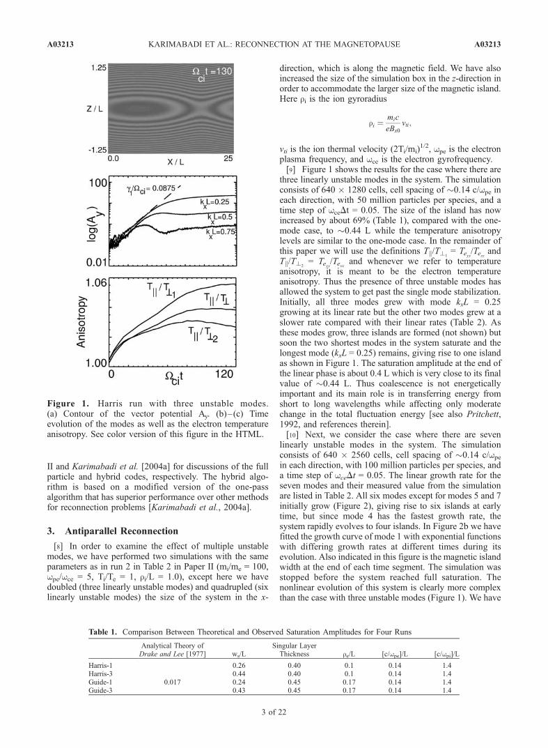
plasma frequency, and wce is the electron gyrofrequency.[9] Figure 1 shows the results for the case where there are

three linearly unstable modes in the system. The simulationconsists of 640 � 1280 cells, cell spacing of �0.14 c/wpe ineach direction, with 50 million particles per species, and atime step of wceDt = 0.05. The size of the island has nowincreased by about 69% (Table 1), compared with the one-mode case, to �0.44 L while the temperature anisotropylevels are similar to the one-mode case. In the remainder ofthis paper we will use the definitions Tk/T?1

= Teyy/Tezz andTk/T?2

= Teyy/Texx and whenever we refer to temperatureanisotropy, it is meant to be the electron temperatureanisotropy. Thus the presence of three unstable modes hasallowed the system to get past the single mode stabilization.Initially, all three modes grew with mode kxL = 0.25growing at its linear rate but the other two modes grew at aslower rate compared with their linear rates (Table 2). Asthese modes grow, three islands are formed (not shown) butsoon the two shortest modes in the system saturate and thelongest mode (kxL = 0.25) remains, giving rise to one islandas shown in Figure 1. The saturation amplitude at the end ofthe linear phase is about 0.4 L which is very close to its finalvalue of �0.44 L. Thus coalescence is not energeticallyimportant and its main role is in transferring energy fromshort to long wavelengths while affecting only moderatechange in the total fluctuation energy [see also Pritchett,1992, and references therein].[10] Next, we consider the case where there are seven

linearly unstable modes in the system. The simulationconsists of 640 � 2560 cells, cell spacing of �0.14 c/wpe

in each direction, with 100 million particles per species, anda time step of wceDt = 0.05. The linear growth rate for theseven modes and their measured value from the simulationare listed in Table 2. All six modes except for modes 5 and 7initially grow (Figure 2), giving rise to six islands at earlytime, but since mode 4 has the fastest growth rate, thesystem rapidly evolves to four islands. In Figure 2b we havefitted the growth curve of mode 1 with exponential functionswith differing growth rates at different times during itsevolution. Also indicated in this figure is the magnetic islandwidth at the end of each time segment. The simulation wasstopped before the system reached full saturation. Thenonlinear evolution of this system is clearly more complexthan the case with three unstable modes (Figure 1). We have

Figure 1. Harris run with three unstable modes.(a) Contour of the vector potential Ay. (b)–(c) Timeevolution of the modes as well as the electron temperatureanisotropy. See color version of this figure in the HTML.

Table 1. Comparison Between Theoretical and Observed Saturation Amplitudes for Four Runs

Analytical Theory ofDrake and Lee [1977] ws/L

Singular LayerThickness re/L [c/wpe]/L [c/wpi]/L

Harris-1 0.26 0.40 0.1 0.14 1.4Harris-3 0.44 0.40 0.1 0.14 1.4Guide-1 0.017 0.24 0.45 0.17 0.14 1.4Guide-3 0.43 0.45 0.17 0.14 1.4


3 of 22

A03213

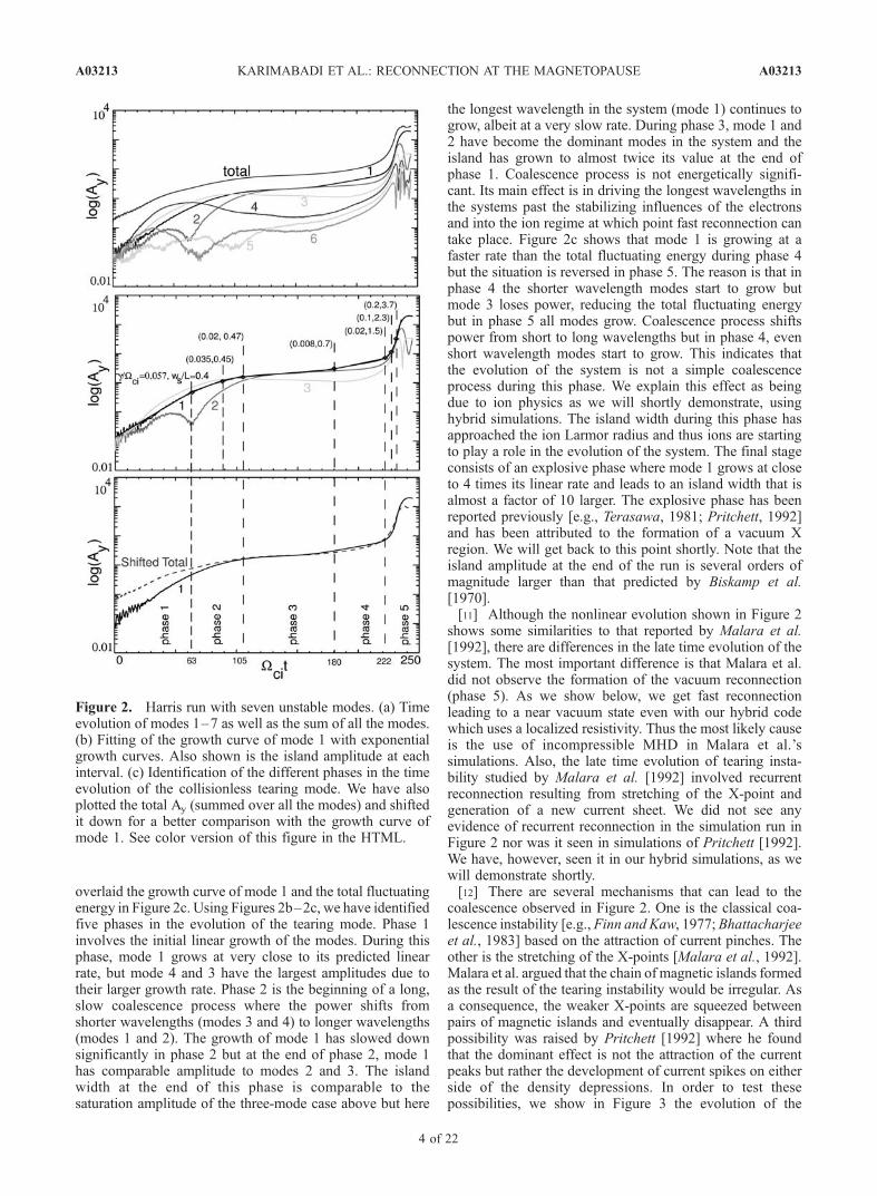
overlaid the growth curve of mode 1 and the total fluctuatingenergy in Figure 2c. Using Figures 2b–2c, we have identifiedfive phases in the evolution of the tearing mode. Phase 1involves the initial linear growth of the modes. During thisphase, mode 1 grows at very close to its predicted linearrate, but mode 4 and 3 have the largest amplitudes due totheir larger growth rate. Phase 2 is the beginning of a long,slow coalescence process where the power shifts fromshorter wavelengths (modes 3 and 4) to longer wavelengths(modes 1 and 2). The growth of mode 1 has slowed downsignificantly in phase 2 but at the end of phase 2, mode 1has comparable amplitude to modes 2 and 3. The islandwidth at the end of this phase is comparable to thesaturation amplitude of the three-mode case above but here

the longest wavelength in the system (mode 1) continues togrow, albeit at a very slow rate. During phase 3, mode 1 and2 have become the dominant modes in the system and theisland has grown to almost twice its value at the end ofphase 1. Coalescence process is not energetically signifi-cant. Its main effect is in driving the longest wavelengths inthe systems past the stabilizing influences of the electronsand into the ion regime at which point fast reconnection cantake place. Figure 2c shows that mode 1 is growing at afaster rate than the total fluctuating energy during phase 4but the situation is reversed in phase 5. The reason is that inphase 4 the shorter wavelength modes start to grow butmode 3 loses power, reducing the total fluctuating energybut in phase 5 all modes grow. Coalescence process shiftspower from short to long wavelengths but in phase 4, evenshort wavelength modes start to grow. This indicates thatthe evolution of the system is not a simple coalescenceprocess during this phase. We explain this effect as beingdue to ion physics as we will shortly demonstrate, usinghybrid simulations. The island width during this phase hasapproached the ion Larmor radius and thus ions are startingto play a role in the evolution of the system. The final stageconsists of an explosive phase where mode 1 grows at closeto 4 times its linear rate and leads to an island width that isalmost a factor of 10 larger. The explosive phase has beenreported previously [e.g., Terasawa, 1981; Pritchett, 1992]and has been attributed to the formation of a vacuum Xregion. We will get back to this point shortly. Note that theisland amplitude at the end of the run is several orders ofmagnitude larger than that predicted by Biskamp et al.[1970].[11] Although the nonlinear evolution shown in Figure 2

shows some similarities to that reported by Malara et al.[1992], there are differences in the late time evolution of thesystem. The most important difference is that Malara et al.did not observe the formation of the vacuum reconnection(phase 5). As we show below, we get fast reconnectionleading to a near vacuum state even with our hybrid codewhich uses a localized resistivity. Thus the most likely causeis the use of incompressible MHD in Malara et al.’ssimulations. Also, the late time evolution of tearing insta-bility studied by Malara et al. [1992] involved recurrentreconnection resulting from stretching of the X-point andgeneration of a new current sheet. We did not see anyevidence of recurrent reconnection in the simulation run inFigure 2 nor was it seen in simulations of Pritchett [1992].We have, however, seen it in our hybrid simulations, as wewill demonstrate shortly.[12] There are several mechanisms that can lead to the

coalescence observed in Figure 2. One is the classical coa-lescence instability [e.g., Finn and Kaw, 1977; Bhattacharjeeet al., 1983] based on the attraction of current pinches. Theother is the stretching of the X-points [Malara et al., 1992].Malara et al. argued that the chain of magnetic islands formedas the result of the tearing instability would be irregular. Asa consequence, the weaker X-points are squeezed betweenpairs of magnetic islands and eventually disappear. A thirdpossibility was raised by Pritchett [1992] where he foundthat the dominant effect is not the attraction of the currentpeaks but rather the development of current spikes on eitherside of the density depressions. In order to test thesepossibilities, we show in Figure 3 the evolution of the

Figure 2. Harris run with seven unstable modes. (a) Timeevolution of modes 1–7 as well as the sum of all the modes.(b) Fitting of the growth curve of mode 1 with exponentialgrowth curves. Also shown is the island amplitude at eachinterval. (c) Identification of the different phases in the timeevolution of the collisionless tearing mode. We have alsoplotted the total Ay (summed over all the modes) and shiftedit down for a better comparison with the growth curve ofmode 1. See color version of this figure in the HTML.


4 of 22

A03213

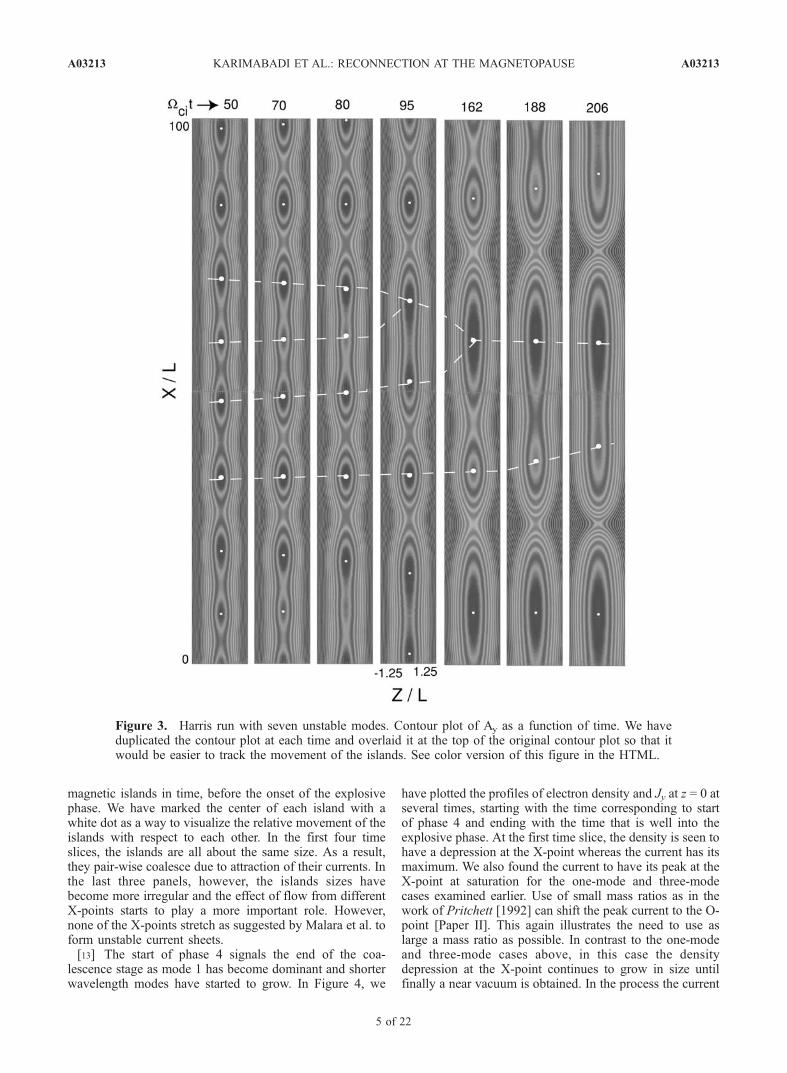
magnetic islands in time, before the onset of the explosivephase. We have marked the center of each island with awhite dot as a way to visualize the relative movement of theislands with respect to each other. In the first four timeslices, the islands are all about the same size. As a result,they pair-wise coalesce due to attraction of their currents. Inthe last three panels, however, the islands sizes havebecome more irregular and the effect of flow from differentX-points starts to play a more important role. However,none of the X-points stretch as suggested by Malara et al. toform unstable current sheets.[13] The start of phase 4 signals the end of the coa-

lescence stage as mode 1 has become dominant and shorterwavelength modes have started to grow. In Figure 4, we

have plotted the profiles of electron density and Jy at z = 0 atseveral times, starting with the time corresponding to startof phase 4 and ending with the time that is well into theexplosive phase. At the first time slice, the density is seen tohave a depression at the X-point whereas the current has itsmaximum. We also found the current to have its peak at theX-point at saturation for the one-mode and three-modecases examined earlier. Use of small mass ratios as in thework of Pritchett [1992] can shift the peak current to the O-point [Paper II]. This again illustrates the need to use aslarge a mass ratio as possible. In contrast to the one-modeand three-mode cases above, in this case the densitydepression at the X-point continues to grow in size untilfinally a near vacuum is obtained. In the process the current

Figure 3. Harris run with seven unstable modes. Contour plot of Ay as a function of time. We haveduplicated the contour plot at each time and overlaid it at the top of the original contour plot so that itwould be easier to track the movement of the islands. See color version of this figure in the HTML.


5 of 22

A03213

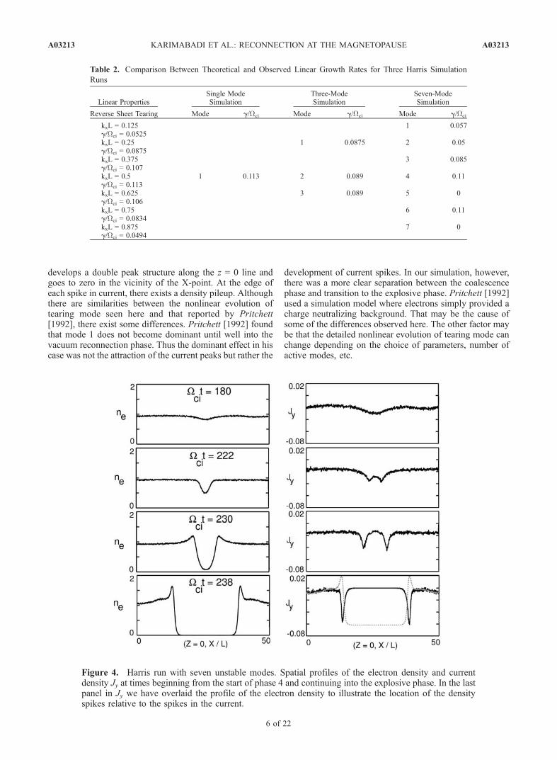
develops a double peak structure along the z = 0 line andgoes to zero in the vicinity of the X-point. At the edge ofeach spike in current, there exists a density pileup. Althoughthere are similarities between the nonlinear evolution oftearing mode seen here and that reported by Pritchett[1992], there exist some differences. Pritchett [1992] foundthat mode 1 does not become dominant until well into thevacuum reconnection phase. Thus the dominant effect in hiscase was not the attraction of the current peaks but rather the

development of current spikes. In our simulation, however,there was a more clear separation between the coalescencephase and transition to the explosive phase. Pritchett [1992]used a simulation model where electrons simply provided acharge neutralizing background. That may be the cause ofsome of the differences observed here. The other factor maybe that the detailed nonlinear evolution of tearing mode canchange depending on the choice of parameters, number ofactive modes, etc.

Table 2. Comparison Between Theoretical and Observed Linear Growth Rates for Three Harris Simulation

Runs

Linear PropertiesSingle ModeSimulation

Three-ModeSimulation

Seven-ModeSimulation

Reverse Sheet Tearing Mode g/Wci Mode g/Wci Mode g/Wci

kxL = 0.125 1 0.057g/Wci = 0.0525kxL = 0.25 1 0.0875 2 0.05g/Wci = 0.0875kxL = 0.375 3 0.085g/Wci = 0.107kxL = 0.5 1 0.113 2 0.089 4 0.11g/Wci = 0.113kxL = 0.625 3 0.089 5 0g/Wci = 0.106kxL = 0.75 6 0.11g/Wci = 0.0834kxL = 0.875 7 0g/Wci = 0.0494

Figure 4. Harris run with seven unstable modes. Spatial profiles of the electron density and currentdensity Jy at times beginning from the start of phase 4 and continuing into the explosive phase. In the lastpanel in Jy we have overlaid the profile of the electron density to illustrate the location of the densityspikes relative to the spikes in the current.


6 of 22

A03213

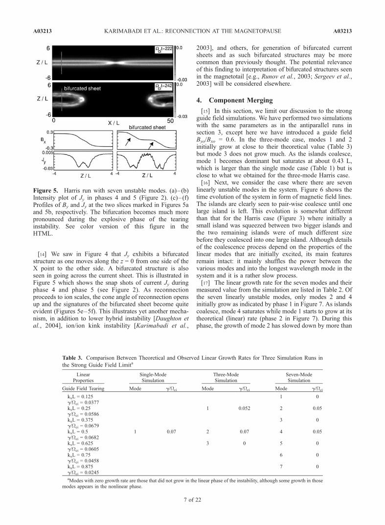
[14] We saw in Figure 4 that Jy exhibits a bifurcatedstructure as one moves along the z = 0 from one side of theX point to the other side. A bifurcated structure is alsoseen in going across the current sheet. This is illustrated inFigure 5 which shows the snap shots of current Jy duringphase 4 and phase 5 (see Figure 2). As reconnectionproceeds to ion scales, the cone angle of reconnection opensup and the signatures of the bifurcated sheet become quiteevident (Figures 5e–5f). This illustrates yet another mecha-nism, in addition to lower hybrid instability [Daughton etal., 2004], ion/ion kink instability [Karimabadi et al.,

2003], and others, for generation of bifurcated currentsheets and as such bifurcated structures may be morecommon than previously thought. The potential relevanceof this finding to interpretation of bifurcated structures seenin the magnetotail [e.g., Runov et al., 2003; Sergeev et al.,2003] will be considered elsewhere.

4. Component Merging

[15] In this section, we limit our discussion to the strongguide field simulations. We have performed two simulationswith the same parameters as in the antiparallel runs insection 3, except here we have introduced a guide fieldByo/Bxo = 0.6. In the three-mode case, modes 1 and 2initially grow at close to their theoretical value (Table 3)but mode 3 does not grow much. As the islands coalesce,mode 1 becomes dominant but saturates at about 0.43 L,which is larger than the single mode case (Table 1) but isclose to what we obtained for the three-mode Harris case.[16] Next, we consider the case where there are seven

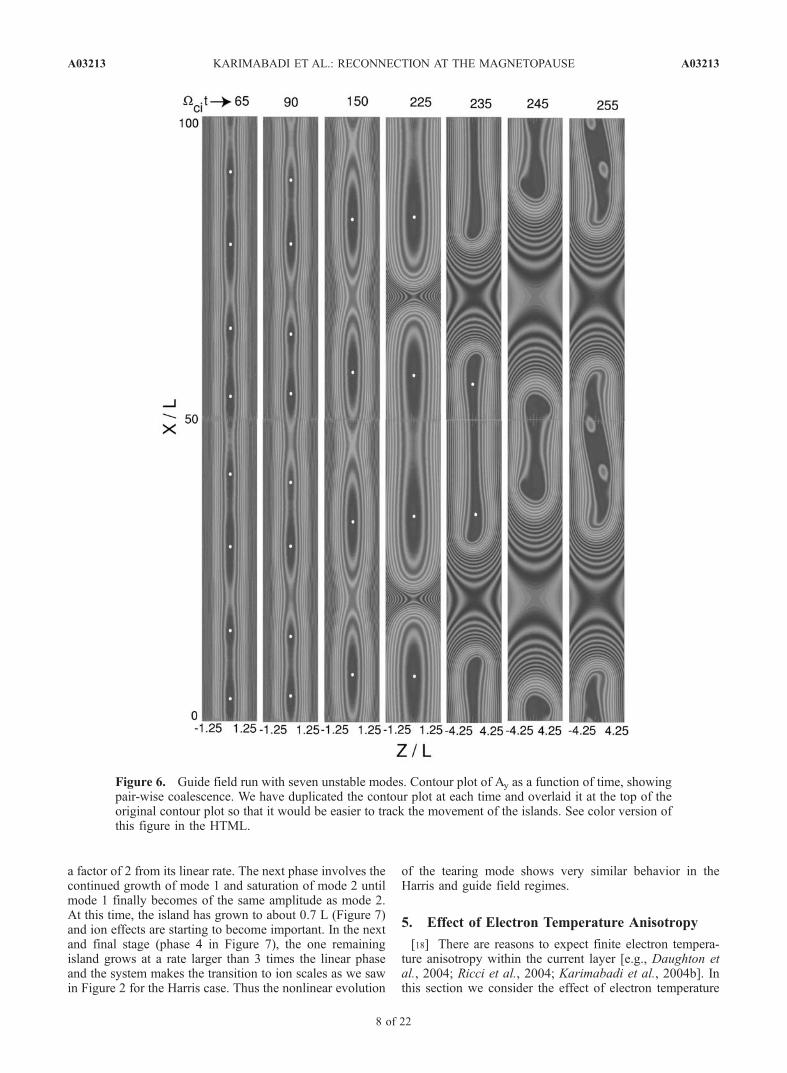
linearly unstable modes in the system. Figure 6 shows thetime evolution of the system in form of magnetic field lines.The islands are clearly seen to pair-wise coalesce until onelarge island is left. This evolution is somewhat differentthan that for the Harris case (Figure 3) where initially asmall island was squeezed between two bigger islands andthe two remaining islands were of much different sizebefore they coalesced into one large island. Although detailsof the coalescence process depend on the properties of thelinear modes that are initially excited, its main featuresremain intact: it mainly shuffles the power between thevarious modes and into the longest wavelength mode in thesystem and it is a rather slow process.[17] The linear growth rate for the seven modes and their

measured value from the simulation are listed in Table 2. Ofthe seven linearly unstable modes, only modes 2 and 4initially grow as indicated by phase 1 in Figure 7. As islandscoalesce, mode 4 saturates while mode 1 starts to grow at itstheoretical (linear) rate (phase 2 in Figure 7). During thisphase, the growth of mode 2 has slowed down by more than

Figure 5. Harris run with seven unstable modes. (a)–(b)Intensity plot of Jy in phases 4 and 5 (Figure 2). (c)–(f)Profiles of By and Jy at the two slices marked in Figures 5aand 5b, respectively. The bifurcation becomes much morepronounced during the explosive phase of the tearinginstability. See color version of this figure in theHTML.

Table 3. Comparison Between Theoretical and Observed Linear Growth Rates for Three Simulation Runs in

the Strong Guide Field Limita

LinearProperties

Single-ModeSimulation

Three-ModeSimulation

Seven-ModeSimulation

Guide Field Tearing Mode g/Wci Mode g/Wci Mode g/Wci

kxL = 0.125 1 0g/Wci = 0.0377kxL = 0.25 1 0.052 2 0.05g/Wci = 0.0586kxL = 0.375 3 0g/Wci = 0.0679kxL = 0.5 1 0.07 2 0.07 4 0.05g/Wci = 0.0682kxL = 0.625 3 0 5 0g/Wci = 0.0605kxL = 0.75 6 0g/Wci = 0.0458kxL = 0.875 7 0g/Wci = 0.0245aModes with zero growth rate are those that did not grow in the linear phase of the instability, although some growth in those

modes appears in the nonlinear phase.


7 of 22

A03213

a factor of 2 from its linear rate. The next phase involves thecontinued growth of mode 1 and saturation of mode 2 untilmode 1 finally becomes of the same amplitude as mode 2.At this time, the island has grown to about 0.7 L (Figure 7)and ion effects are starting to become important. In the nextand final stage (phase 4 in Figure 7), the one remainingisland grows at a rate larger than 3 times the linear phaseand the system makes the transition to ion scales as we sawin Figure 2 for the Harris case. Thus the nonlinear evolution

of the tearing mode shows very similar behavior in theHarris and guide field regimes.

5. Effect of Electron Temperature Anisotropy

[18] There are reasons to expect finite electron tempera-ture anisotropy within the current layer [e.g., Daughton etal., 2004; Ricci et al., 2004; Karimabadi et al., 2004b]. Inthis section we consider the effect of electron temperature

Figure 6. Guide field run with seven unstable modes. Contour plot of Ay as a function of time, showingpair-wise coalescence. We have duplicated the contour plot at each time and overlaid it at the top of theoriginal contour plot so that it would be easier to track the movement of the islands. See color version ofthis figure in the HTML.


8 of 22

A03213

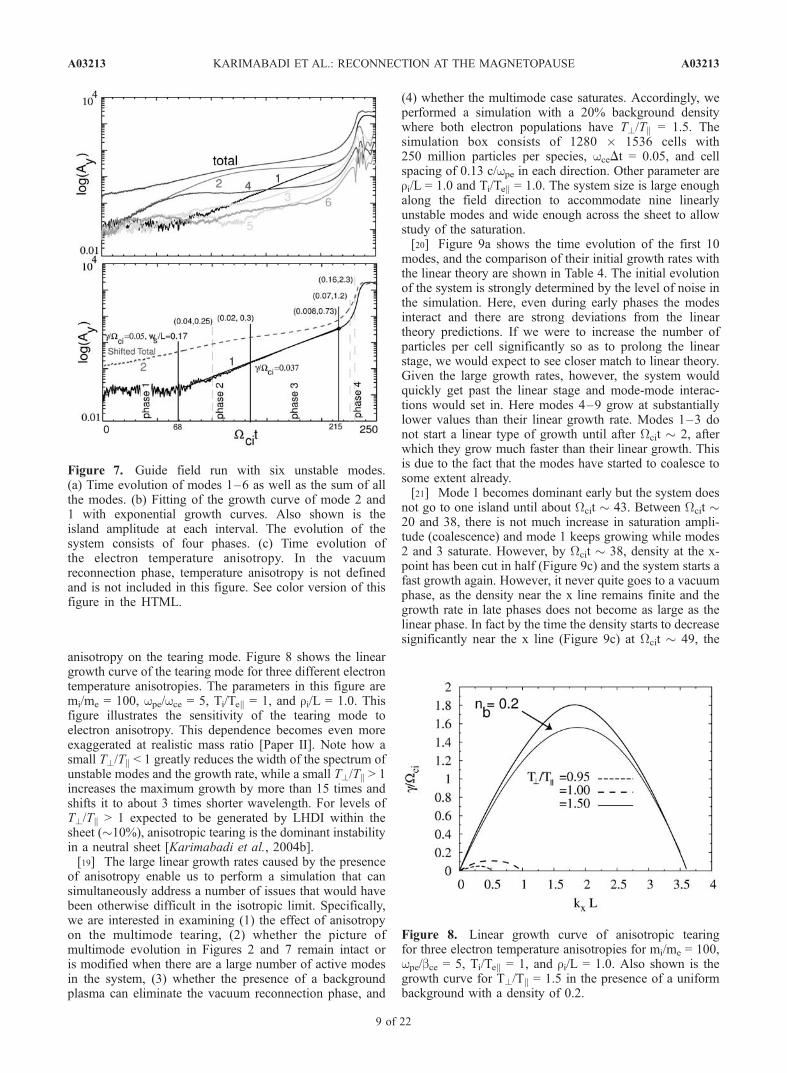
anisotropy on the tearing mode. Figure 8 shows the lineargrowth curve of the tearing mode for three different electrontemperature anisotropies. The parameters in this figure aremi/me = 100, wpe/wce = 5, Ti/Tek = 1, and ri/L = 1.0. Thisfigure illustrates the sensitivity of the tearing mode toelectron anisotropy. This dependence becomes even moreexaggerated at realistic mass ratio [Paper II]. Note how asmall T?/Tk < 1 greatly reduces the width of the spectrum ofunstable modes and the growth rate, while a small T?/Tk > 1increases the maximum growth by more than 15 times andshifts it to about 3 times shorter wavelength. For levels ofT?/Tk > 1 expected to be generated by LHDI within thesheet (�10%), anisotropic tearing is the dominant instabilityin a neutral sheet [Karimabadi et al., 2004b].[19] The large linear growth rates caused by the presence

of anisotropy enable us to perform a simulation that cansimultaneously address a number of issues that would havebeen otherwise difficult in the isotropic limit. Specifically,we are interested in examining (1) the effect of anisotropyon the multimode tearing, (2) whether the picture ofmultimode evolution in Figures 2 and 7 remain intact oris modified when there are a large number of active modesin the system, (3) whether the presence of a backgroundplasma can eliminate the vacuum reconnection phase, and

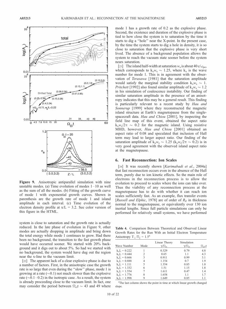
(4) whether the multimode case saturates. Accordingly, weperformed a simulation with a 20% background densitywhere both electron populations have T?/Tk = 1.5. Thesimulation box consists of 1280 � 1536 cells with250 million particles per species, wceDt = 0.05, and cellspacing of 0.13 c/wpe in each direction. Other parameter areri/L = 1.0 and Ti/Tek = 1.0. The system size is large enoughalong the field direction to accommodate nine linearlyunstable modes and wide enough across the sheet to allowstudy of the saturation.[20] Figure 9a shows the time evolution of the first 10

modes, and the comparison of their initial growth rates withthe linear theory are shown in Table 4. The initial evolutionof the system is strongly determined by the level of noise inthe simulation. Here, even during early phases the modesinteract and there are strong deviations from the lineartheory predictions. If we were to increase the number ofparticles per cell significantly so as to prolong the linearstage, we would expect to see closer match to linear theory.Given the large growth rates, however, the system wouldquickly get past the linear stage and mode-mode interac-tions would set in. Here modes 4–9 grow at substantiallylower values than their linear growth rate. Modes 1–3 donot start a linear type of growth until after Wcit � 2, afterwhich they grow much faster than their linear growth. Thisis due to the fact that the modes have started to coalesce tosome extent already.[21] Mode 1 becomes dominant early but the system does

not go to one island until about Wcit � 43. Between Wcit �20 and 38, there is not much increase in saturation ampli-tude (coalescence) and mode 1 keeps growing while modes2 and 3 saturate. However, by Wcit � 38, density at the x-point has been cut in half (Figure 9c) and the system starts afast growth again. However, it never quite goes to a vacuumphase, as the density near the x line remains finite and thegrowth rate in late phases does not become as large as thelinear phase. In fact by the time the density starts to decreasesignificantly near the x line (Figure 9c) at Wcit � 49, the

Figure 7. Guide field run with six unstable modes.(a) Time evolution of modes 1–6 as well as the sum of allthe modes. (b) Fitting of the growth curve of mode 2 and1 with exponential growth curves. Also shown is theisland amplitude at each interval. The evolution of thesystem consists of four phases. (c) Time evolution ofthe electron temperature anisotropy. In the vacuumreconnection phase, temperature anisotropy is not definedand is not included in this figure. See color version of thisfigure in the HTML.

Figure 8. Linear growth curve of anisotropic tearingfor three electron temperature anisotropies for mi/me = 100,wpe/bce = 5, Ti/Tek = 1, and ri/L = 1.0. Also shown is thegrowth curve for T?/Tk = 1.5 in the presence of a uniformbackground with a density of 0.2.


9 of 22

A03213

system is close to saturation and the growth rate is actuallyreduced. In the late phase of evolution in Figure 9, othermodes are actually dropping in amplitude and bring downthe total energy while mode 1 continues to grow. Had therebeen no background, the transition to the fast growth phasewould have occurred sooner. We started with 20% back-ground and it digs out to about 5%. So had we started withno background, the system would have dug out the regionnear the x-line to the vacuum limit.[22] The apparent lack of a clear explosive phase is due to

a number of factors. First, in the anisotropic case the growthrate is so large that even during the ‘‘slow’’ phase, mode 1 isgrowing at a rate (�0.1) not much slower than the explosiverate (�0.1–0.2) in the isotropic case. As a result, the systemis already proceeding close to the vacuum limit. In fact, onemay consider the period between Wcit � 43 and 49 where

mode 1 has a growth rate of 0.2 as the explosive phase.Second, the existence and duration of the explosive phase istied to how close the system is to saturation by the time itstarts to dig a ‘‘hole’’ near the X-point. In the present case,by the time the system starts to dig a hole in density, it is soclose to saturation that the explosive phase is very shortlived. The absence of a background population allows thesystem to reach the vacuum state sooner before the systemnears saturation.[23] The island half-width at saturationws is about 40 c/wpe,

which corresponds to kxws � 1.25, where kx is the wavenumber for mode 1. This is in agreement with the obser-vation of Terasawa [1981] that the saturation amplitudewould satisfy the marginal stability condition kxws � 1.Pritchett [1992] also found similar amplitude of kxws � 1.2in his simulation of coalescence instability. Our finding ofsimilar saturation amplitude in the presence of an anisot-ropy indicates that this may be a general result. This findingis particularly relevant to a recent study by Hau andSonnerup [1999] where they reconstructed the magneticisland structure at Earth’s magnetopause from the single-spacecraft data. Hau and Chiou [2001], by inspecting thefield line map of this event, obtained the aspect ratiokxws/2p � 0.2 for the magnetic island. Using resistiveMHD, however, Hau and Chiou [2001] obtained anaspect ratio of 0.08 and speculated that inclusion of Hallterm may lead to larger aspect ratio. Our finding of thesaturation amplitude of kxws � 1.25 (kxws/2p � 0.2) is invery good agreement with the observed island aspect ratioat the magnetopause.

6. Fast Reconnection: Ion Scales

[24] It was recently shown [Karimabadi et al., 2004a]that fast reconnection occurs even in the absence of the Hallterm, purely due to ion kinetic effects. So the main role ofelectrons in the reconnection process is to allow theevolution to proceed to scales where the ions can take over.Thus the viability of any reconnection process at themagnetopause has to do with whether it can reach ionscales sufficiently fast. As an example, flux transfer events[Russell and Elphic, 1978] are of order of RE in thicknessnormal to the magnetopause, or equivalently over 130 ioninertial lengths. Since full particle simulations can only beperformed for relatively small systems, we have performed

Figure 9. Anisotropic antiparallel simulation with nineunstable modes. (a) Time evolution of modes 1–10 as wellas the sum of all the modes. (b) Fitting of the growth curveof mode 1 with exponential growth curves. Shown inparenthesis are the growth rate of mode 1 and islandamplitude in each interval. (c) Time evolution of theelectron density profile at x/L = 3.2. See color version ofthis figure in the HTML.

Table 4. Comparison Between Theoretical and Observed Linear

Growth Rates for the Run With an Initial Electron Temperature

Anisotropy T?/Tk = 1.5a

Wave Number ModeLinear Theory

g/Wci

Simulationg/Wci Wci*t

kxL = 0.222 1 0.329 0.79 4.8kxL = 0.444 2 0.65 1.1 4.3kxL = 0.666 3 0.911 0.99 3.1kxL = 0.888 4 1.154 0.7 1.9kxL = 1.111 5 1.354 0.85 1.0kxL = 1.332 6 1.51 1.15 1.8kxL = 1.554 7 1.611 0.47 1.4kxL = 1.776 8 1.658 1.1 1.7kxL = 1.998 9 1.649 0.85 1.1aThe last column shows the point in time at which linear growth changed

slope.


10 of 22

A03213

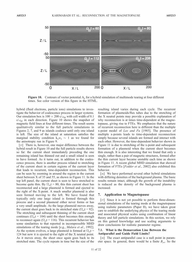
hybrid (fluid electrons, particle ions) simulations to inves-tigate the behavior of coalescence process in larger systems.Our simulation box is 100 � 200 c/wpi with cell width of 0.1c/wpi in each direction. Figure 10 shows the snapshot ofmagnetic field lines at four different times. The result seemsqualitatively similar to the full particle simulations inFigures 2, 7, and 9 as islands coalesce until only one islandis left. The size of the island at saturation satisfies themarginal stability condition kxws � 1 as we found forthe anisotropic run in Figure 9.[25] There is, however, one major difference between the

hybrid result in Figure 10 and the full particle results shownso far: the current sheet immediately preceding the oneremaining island has thinned out and a small island is seento have formed. As it turns out, in addition to the coales-cence process, there is another process related to stretchingof the current sheet in certain regions of the current layerthat leads to recurrent, time-dependent reconnection. Thiscan be seen by zooming in around the region in the currentsheet between X of 35 and 55, as shown in Figure 11. In thetop left panel, the current sheet is seen to have stretched tobecome quite thin. By Wcit = 80, this thin current sheet hasreconnected and a large plasmoid is formed and ejected tothe right of the X-point. A much smaller plasmoid is alsoseen formed moving to the left. We have found thattypically only one large island is formed through thisprocess and a second plasmoid either never forms or hasa very small amplitude. As the large plasmoid moves away,the current sheet goes back to its stretched state (Wcit = 92).The stretching and subsequent thinning of the current sheetcontinues (Wcit = 104) until the sheet becomes thin enoughto reconnect again (Wcit = 116). This recurrent behavior hassome similarities to that reported in incompressible MHDsimulations of the tearing mode [e.g., Malara et al., 1992].As the system evolves, a large plasmoid is formed at Wcit =124 but now it is ejected to the right of the X neutral point.As it moves away, the sheet once again goes back to itsstretched state. The cycle repeats in time but the size of the

resulting island varies during each cycle. The recurrentformation of plasmoids/flux tubes due to the stretching ofthe X neutral points may provide a possible explanation ofwhy reconnection is at times time-dependent at the magne-topause, giving rise to FTEs. We emphasize that the natureof recurrent reconnection here is different than the multiplex-point model of Lee and Fu [1985]. The presence ofmultiple x-points leads to time-dependent reconnectionsimply because several islands are formed and interact witheach other. However, the time-dependent behavior shown inFigure 11 is due to stretching of the x-point and subsequentformation of a plasmoid when the current sheet becomesthin enough. It is also interesting that we found that only asingle, rather than a pair of magnetic structures, formed afterthe thin current layer became unstable each time as shownin Figure 11. A recent global MHD simulation that showedformation of FTEs [Fedder et al., 2002] also exhibited thisbehavior.[26] We have performed several other hybrid simulations

with differing densities of the background plasma. The basicresults remain intact, although the growth of the instabilityis reduced as the density of the background plasma isincreased.

7. Application to Magnetopause

[27] Since it is not yet possible to perform three-dimen-sional simulations of the tearing mode at the magnetopauseusing realistic parameters (Paper II), we have taken greatcare to establish the underlying physics of the tearing modeand associated physical scales using combination of lineartheory and full particle simulations. In this section, we relyon this gained knowledge and use scaling arguments todraw conclusions for realistic parameter regime.

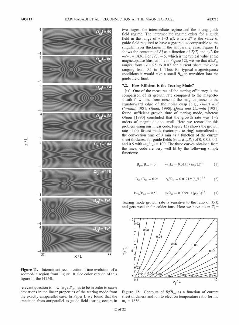
7.1. What is the Demarcation Line Between theAntiparallel and Guide Field Limits?

[28] The exact antiparallel case is a null point in param-eter space. In general, there would be a finite Byo. So the

Figure 10. Contours of vector potential Ay for a hybrid simulation of multimode tearing at four differenttimes. See color version of this figure in the HTML.


11 of 22

A03213

relevant question is how large Byo has to be in order to causedeviations in the linear properties of the tearing mode fromthe exactly antiparallel case. In Paper I, we found that thetransition from antiparallel to guide field tearing occurs in

two stages, the intermediate regime and the strong guidefield regime. The intermediate regime exists for a guidefield in the range of �1–3 B*y, where B*y is the value ofguide field required to have a gyroradius comparable to thesingular layer thickness in the antiparallel case. Figure 12shows the contours of B*y as a function of Ti/Te and ri/L formi/me = 1836. For Ti/Te � 5, which is the typical value at themagnetopause (dashed line in Figure 12), we see that B*y /Bxo

ranges from �0.025 to 0.07 for current sheet thicknessranging from 0.1 to 1. Thus for typical magnetopauseconditions it would take a small Byo to transition into theguide field limit.

7.2. How Efficient is the Tearing Mode?

[29] One of the measures of the tearing efficiency is thecomparison of its growth rate compared to the magneto-sheath flow time from nose of the magnetopause to theequatorward edge of the polar cusp [e.g., Quest andCoroniti, 1981; Gladd, 1990]. Quest and Coroniti [1981]found sufficient growth time of tearing mode, whereasGladd [1990] concluded that the growth rate was 1–2orders of magnitude too small. Here we reconsider thisproblem using our linear code. Figure 13a shows the growthrate of the fastest mode (isotoropic tearing) normalized tothe convection time of 3 min as a function of the currentsheet thickness for guide fields (a � Byo/Bo) of 0, 0.05, 0.2,and 0.5 with wpe/wce = 100. The three curves obtained fromthe linear code are very well fit by the following simplefunctions:

Byo=Bxo ¼ 0: g=Wci ¼ 0:0351 * ri=Lð Þ2:3 ð1Þ

Byo=Bxo ¼ 0:2: g=Wci ¼ 0:0171 * ri=Lð Þ2:6 ð2Þ

Byo=Bxo ¼ 0:5: g=Wci ¼ 0:00991 * ri=Lð Þ2:9: ð3Þ

Tearing mode growth rate is sensitive to the ratio of Ti/Teand gets weaker for colder ions. Here we have taken Ti =

Figure 11. Intermittent reconnection. Time evolution of azoomed-in region from Figure 10. See color version of thisfigure in the HTML.

Figure 12. Contours of B*y/Bxo as a function of currentsheet thickness and ion to electron temperature ratio for mi/me = 1836.


12 of 22

A03213

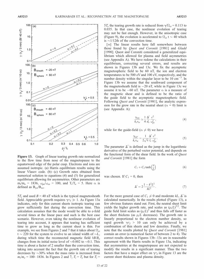
5Te and used B = 40 nT which is the typical magnetosheathfield. Appreciable growth requires gtf � 1. As Figure 13aindicates, only for thin current sheets isotropic tearing cangrow sufficiently fast during the convection time. Thiscalculation assumes that the mode would be able to e-foldseveral times at the linear pace and such is the best casescenario. However, even taking the nonlinear evolution oftearing into account, it appears that tearing has sufficienttime to grow as long as the current sheet is thin. Forexample, we see from Figures 2 and 7 that it takes about Wci

t � 220 for the system to evolve to an island width of �L,during which time the reconnected magnetic field dB/Bo

changes from its initial noise level of �0.002 to �0.1. Thistime is about a factor of 2 smaller than the convection time,taking into account the fact that the growth rate of tearingdecreases by �30% when the mass ratio is increased frommi/me = 100–1836. In Figures 2 and 7, Ti = Te but for Ti =

5Te the tearing growth rate is reduced from g/Wci = 0.113 to0.035. In that case, the nonlinear evolution of tearingmay not be fast enough. However, in the anisotropic case(Figure 9), the evolution is accelerated to Wci t � 40 whichis �1/12th of the convection time.[30] The linear results here fall somewhere between

those found by Quest and Coroniti [1981] and Gladd[1990]. Quest and Coroniti considered a generalized equi-librium which allowed for plasma and field asymmetries(see Appendix A). We have redone the calculations in theirequilibrium, correcting several errors, and results areshown in Figures 13b and 13c. We fix the asymptoticmagnetospheric field to be 60 nT, the ion and electrontemperatures to be 500 eV and 100 eV, respectively, and thenumber density within the singular layer to be 10 cm�3. InFigure 13b we assume that the southward component ofthe magnetosheath field is �20 nT, while in Figure 13c weassume it to be �60 nT. The parameter a is a measure ofthe magnetic shear and is defined to be the ratio ofthe guide field to the asymptotic magnetospheric field.Following Quest and Coroniti [1981], the analytic expres-sion for the grow rate in the neutral sheet (a = 0) limit is(see Appendix A):

gNS

kxvte’ 1

4

D0

de

c2

w2pe

; ð4Þ

while for the guide-field (a 6¼ 0) we have

gGF

kxvte¼ 1

2ffiffiffip

p D0

ls

c2

w2pe

: ð5Þ

The parameter D0 is defined as the jump in the logarithmicderivative of the perturbed vector potential, and depends onthe functional form of the shear field. In the work of Questand Coroniti [1981] the form

C1 þ C2 tanhx

L

� �ð6Þ

was chosen. If C1 = 0, then

D0 ¼ 2

1� k2L2

kL2: ð7Þ

For the more general case of C1 6¼ 0 and moderate kL, D0 iscalculated numerically. In the results plotted (Figure 13), afew obvious features stand out. First, the neutral sheet limityields the higher growth rate, and scales as (ri/L)

5/2. Theguide field limit scales as (ri/L)

3 and thus falls off faster asthe sheet thickens (as ri/L decreases). The growth rate islinearly proportional to the electron number density, sorapid growth gtf > 10 can only be achieved by acombination of thin sheets and low densities. Finally, wenote that the results plotted by Quest and Coroniti [1981]contain an error (a numerical factor of between 2 to 4). Thecorrect results shown in Figures 13b–13c are in reasonableagreement with the Harris results in Figure 13a, indicatingthat asymmetries at the magnetopause are not expected tomodify the results in a significant manner. Thus the twofactors that have a major effect on gtf in Figure 13 are thecurrent sheet thickness and plasma density.

Figure 13. Graph of linear tearing growth rate normalizedto the flow time from nose of the magnetopause to theequatorward edge of the polar cusp. Electrons and ions areassumed isotropic. (a) Harris equilibrium results using thelinear Vlasov code. (b)–(c) Growth rates obtained fromnumerical solution to equations (4) and (5) for generalizedequilibrium allowing for asymmetries. Other parameters aremi/me = 1836, wpe/wce = 100, and Ti/Te = 5. Here a isdefined as Byo/Bxo.


13 of 22

A03213

[31] The calculations in Figure 13 are based on isotropicconditions. Although antiparallel regime has faster growth,guide field tearing still provides sufficient growth for thinsheets. Ion anisotropy can increase the growth rate but onlyabout a factor of �2 for thin sheets. Electron anisotropy T?/Tk > 1, however, can significantly increase the growth rateof shorter wavelengths (e.g., Figure 8). Inclusion of electronanisotropy when there is a finite guide field is beyond thescope of this article and will be considered elsewhere.However, its effect is expected to be muted when there is afinite guide field. Thus the presence of any finite electronanisotropy with T?/Tk > 1 could favor antiparallel merging.

7.3. What Island Width is Required to Explain theReconnected Rates at the Magnetopause?

[32] Aside from the linear growth, another measure ofefficiency of the tearing mode is its nonlinear saturation. Ifthe island saturation amplitude is small, then only a smallfraction of magnetopause is open to reconnection and thisleads to very small fraction of particles penetrating themagnetopause. In this section, we use simple argumentsto derive an expression for the reconnected flux and itsrelation to the size of the island. The analysis here is validfor both the zero and finite guide field limits. For simplicity,let us assume a two-dimensional geometry in which thereconnection is restricted to the x-z plane. Further assumethat the x-point is located at x = z = 0. Inflow is in the zdirection, and outflow is in the x direction. Assume usualsymmetries such that Uz(x, 0, t) = Ux(0, z, t) = 0, where U

!is

the electron velocity vector. For MHD, this quantity is alsothe ion velocity vector. We choose the electron velocity as itis more tightly bound to the magnetic field. For the time-dependent problem, a useful quantity is the total magneticflux F(t) (per unit length in the y direction) that has beenreconnected by time t, assuming a tangential discontinuity attime t = 0. We can define it as

F tð Þ ¼Z Lmax

0

Bz x; 0; tð Þdx

¼Z Lmax

0

r� A!� �

� zdx

¼Z Lmax

0

@

@xAy x; 0; tð Þ

¼ Ay Lmax; 0; tð Þ � Ay 0; 0; tð Þ ð8Þ

where Lmax is the maximum size of the system in the x-direction. If we define the reconnection rate as the total fluxper unit time that has been reconnected, we get

d

dtF tð Þ ¼

Z Lmax

0

@

@tBz x; 0; tð Þdx ð9aÞ

¼ �c

Z Lmax

0

r� E!� �

� zdx ð9bÞ

¼ �c

Z Lmax

0

@

@xEy x; 0; tð Þdx ð9cÞ

¼ �cEy Lmax; 0; tð Þ þ cEy 0; 0; tð Þ: ð9dÞ

An alternate way to estimate the reconnection rate is

d

dtF tð Þ ’ F t þ Dtð Þ � F tð Þ

Dtð10aÞ

F tð Þ ¼ Ay Lmax; 0; tð Þ � Ay 0; 0; tð Þ: ð10bÞ

To make the example more concrete, define the magneticfield for the case of a magnetic island. Near the center of aone-dimensional sheared current layer, we can approximatethe equilibrium magnetic field as linear in z (while pointingin x). We then obtain [Paper II] the following expressionsfor the total potential and the island half-width:

Ay zð Þ þ dAy xð Þ ¼ �Bxo

2Lz2 � dBn

kxcos kxxð Þ ð11aÞ

ws

L¼ 2

ffiffiffiffiffiffiffidbkxL

s; ð11bÞ

where we have defined db = dBn/Bxo. The x-pointsare located at kxx = 0 (and kxx = 2p), while the O-point isat kxx = p. Thus the value of the vector potential at thex-point is (x = z = 0) is dAy(0) = �dBn

kx. The reconnected

flux (per unit length y) F can then be obtained as

F tð Þ ¼ dAy p=kxð Þ � Ay 0ð Þ ¼ 2dBn

kx/ ws=Lð Þ2: ð12Þ

Thus the reconnected flux is proportional to the square ofthe half-width of the island. The reconnection rate is lessstraightforward to estimate analytically, since this nowdepends on the time history of the field. If, however, theisland is exponentially growing with a growth rate g, thenwe have

dF tð Þdt

¼ gF tð Þ: ð13Þ

Note that there is an important distinction between thetime-dependent reconnection rate as in (13) and the time-dependent reconnection rate. The latter is affected by boththe linear and nonlinear evolution of the tearing modewhereas the steady state reconnection rate (see nextsection) is not. The time-dependent reconnection rate isgenerally lower in the presence of the guide field becauseboth the linear growth and saturation amplitude aretypically smaller.[33] Reconnection rates are hard to measure at the mag-

netopause. There are several measures of reconnection rate.One is MAn = Vn/VA = db [Paschmann, 1997] and another isthe tangential electric field Et measured in the frame movingwith the magnetopause [Paschmann, 1997]. Lindqvist andMozer [1990], using a statistical study of ISEE data,obtained an average value of Et of 0.4 mV/m and an averageconvection speed of 20 km/s (Alfven speed �120 km/s).This translates to db � 0.07 [Paschmann, 1997]. These arecrude estimates but suffice for our purposes here. Usingdb � 0.07 in (11b) and taking kxL = 0.5, we obtain ws/L �


14 of 22

A03213

0.75. Thus in order to get sufficient reconnection, themagnetic island needs to grow to the scale length of themagnetopause L. In Paper II, we showed that single islandtearing saturates at an amplitude at or below the singularlayer thickness, which is much smaller than L. Thusmultimode tearing is required to reconnect sufficient flux.

7.4. Effect of Guide Field on the Steady StateReconnection Rate

[34] Another way to gauge the viability of componentmerging at the magnetopause is to calculate the steady statereconnection rate (i.e., the rate calculated after the systemhas reached steady state) as a function of guide fieldstrength. In a periodic simulation, the outflow jets thatreach the boundary will start to come into the simulationon the opposite side. Thus, implementation of outflowboundary condition is required to allow the system to reachsteady-state. We calculate the steady state reconnection rateusing a procedure outlined by Karimabadi et al. [2004a].We used two-dimensional (2-D) hybrid simulations of asymmetric tangential discontinuity [Karimabadi et al.,1999] with a system size of 40 � 40 ion inertial length,and a single, localized resistivity of 10�4 (normalized to 4p/wpi) with a cosh profile extending two ion inertial lengths ineach direction. For steady-state reconnection the definitionF(t) = Ay(Lmax, 0, t) � Ay(0, 0, t) is still valid, but not useful.Here an assumption must be made regarding the relation-ship of the plasma motion and the magnetic field. We makethe usual approximation that, away from the diffusionregion, the magnetic flux is ‘‘frozen’’ into the electron fluid.It follows that

d

dtF tð Þ ¼ Bz x; 0ð ÞUx x; 0ð Þ ¼ �cEy x; 0ð Þ: ð14Þ

Note that for a uniform reconnection rate to exist, werequire that Ey(x, z) be constant, independent of position.Finally, given the assumption that the flux and the electronvelocity are tied to each other, an alternate way to define thereconnection rate is to define it as proportional to theasymptotic outflow velocity Ux(x, 0).

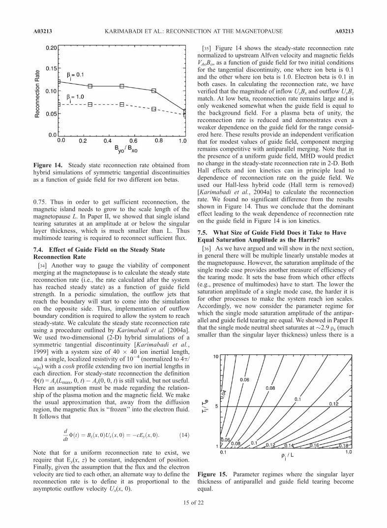
[35] Figure 14 shows the steady-state reconnection ratenormalized to upstream Alfven velocity and magnetic fieldsVAoBo, as a function of guide field for two initial conditionsfor the tangential discontinuity, one where ion beta is 0.1and the other where ion beta is 1.0. Electron beta is 0.1 inboth cases. In calculating the reconnection rate, we haveverified that the magnitude of inflow UzBx and outflow UxBz

match. At low beta, reconnection rate remains large and isonly weakened somewhat when the guide field is equal tothe background field. For a plasma beta of unity, thereconnection rate is reduced and demonstrates even aweaker dependence on the guide field for the range consid-ered here. These results provide an independent verificationthat for modest values of guide field, component mergingremains competitive with antiparallel merging. Note that inthe presence of a uniform guide field, MHD would predictno change in the steady-state reconnection rate in 2-D. BothHall effects and ion kinetics can in principle lead todependence of reconnection rate on the guide field. Weused our Hall-less hybrid code (Hall term is removed)[Karimabadi et al., 2004a] to calculate the reconnectionrate. We found no significant difference from the resultsshown in Figure 14. Thus we conclude that the dominanteffect leading to the weak dependence of reconnection rateon the guide field in Figure 14 is ion kinetics.

7.5. What Size of Guide Field Does it Take to HaveEqual Saturation Amplitude as the Harris?

[36] As we have argued and will show in the next section,in general there will be multiple linearly unstable modes atthe magnetopause. However, the saturation amplitude of thesingle mode case provides another measure of efficiency ofthe tearing mode. It sets the base from which other effects(e.g., presence of multimodes) have to start. The lower thesaturation amplitude of a single mode case, the harder it isfor other processes to make the system reach ion scales.Accordingly, we now consider the parameter regime forwhich the single mode saturation amplitude of the antipar-allel and guide field tearing are equal. We showed in Paper IIthat the single mode neutral sheet saturates at �2.9 re (muchsmaller than the singular layer thickness) unless there is a

Figure 14. Steady state reconnection rate obtained fromhybrid simulations of symmetric tangential discontinuitiesas a function of guide field for two different ion betas.

Figure 15. Parameter regimes where the singular layerthickness of antiparallel and guide field tearing becomeequal.


15 of 22

A03213

mechanism to pitch angle scatter the electrons at whichpoint tearing would saturate at the singular layer thickness.In the guide field case, tearing saturates at the singular layerthickness, independent of the presence of scattering, andsaturation amplitude is �1.8 reG, where reG is the electrongyroradius in the guide field. Let us define the variable z tobe the ratio of saturation amplitude of the antiparallel case tothe singular layer thickness. Then, the guide field for whichthe saturation amplitude of the antiparallel and guide fieldcases become comparable is given by

Bycrit ¼ 1:8=zð ÞB*y; ð15Þ

where z is less than or equal to one. Figure 15 (for mi/me =1836) shows contours of Bycrit

for z = 1. Picking z for aparticular case, this figure can then be used to easilyestimate the guide field for which the two saturationamplitudes would be equal. For example, let use assumethat it turns out that z is 0.5 rather than one forthe parameters corresponding to the contour of 0.18 inFigure 15. That would mean that the guide field forwhich antiparallel and guide field tearing would haveequal saturation amplitudes would be 0.18/z = 0.36. FromFigure 15, it is clear that if there are no mechanisms toincrease the saturation amplitude of the antiparallel caseto the singular layer thickness so that z � 1, then theguide field tearing can have larger saturation amplitude aslong as the guide field is not too strong. Even for z � 1,guide field tearing optimal region would remain compe-titive to antiparallel tearing for ri/L � 0.5–1. In summary,antiparallel merging in 2-D would have z < 1 and guidefield tearing would be competitive unless the guide fieldis too strong.

7.6. How Many Modes Can Fit at the Magnetopause?

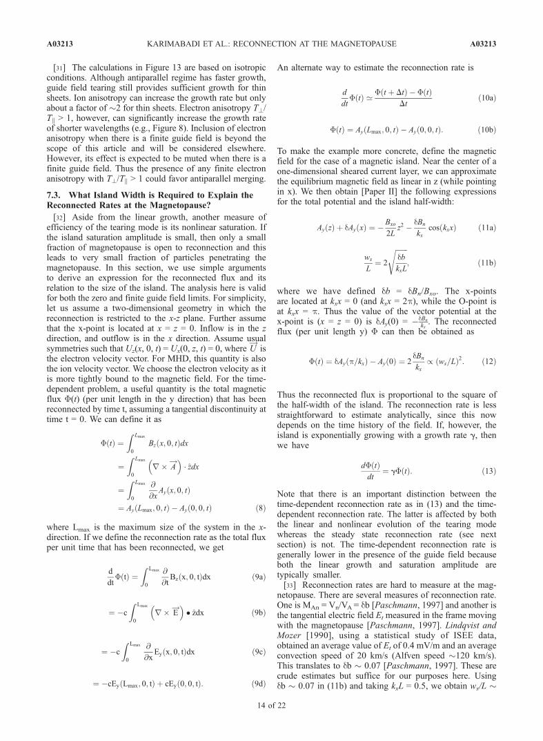
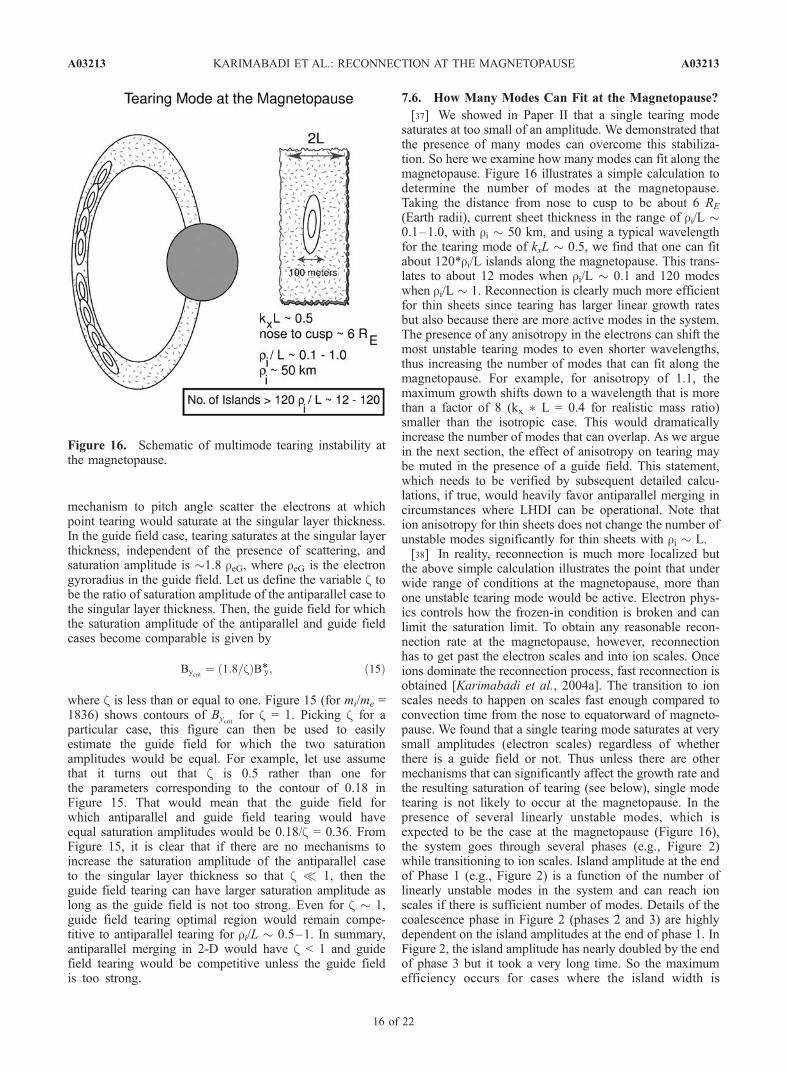
[37] We showed in Paper II that a single tearing modesaturates at too small of an amplitude. We demonstrated thatthe presence of many modes can overcome this stabiliza-tion. So here we examine how many modes can fit along themagnetopause. Figure 16 illustrates a simple calculation todetermine the number of modes at the magnetopause.Taking the distance from nose to cusp to be about 6 RE

(Earth radii), current sheet thickness in the range of ri/L �0.1–1.0, with ri � 50 km, and using a typical wavelengthfor the tearing mode of kxL � 0.5, we find that one can fitabout 120*ri/L islands along the magnetopause. This trans-lates to about 12 modes when ri/L � 0.1 and 120 modeswhen ri/L � 1. Reconnection is clearly much more efficientfor thin sheets since tearing has larger linear growth ratesbut also because there are more active modes in the system.The presence of any anisotropy in the electrons can shift themost unstable tearing modes to even shorter wavelengths,thus increasing the number of modes that can fit along themagnetopause. For example, for anisotropy of 1.1, themaximum growth shifts down to a wavelength that is morethan a factor of 8 (kx � L = 0.4 for realistic mass ratio)smaller than the isotropic case. This would dramaticallyincrease the number of modes that can overlap. As we arguein the next section, the effect of anisotropy on tearing maybe muted in the presence of a guide field. This statement,which needs to be verified by subsequent detailed calcu-lations, if true, would heavily favor antiparallel merging incircumstances where LHDI can be operational. Note thation anisotropy for thin sheets does not change the number ofunstable modes significantly for thin sheets with ri � L.[38] In reality, reconnection is much more localized but

the above simple calculation illustrates the point that underwide range of conditions at the magnetopause, more thanone unstable tearing mode would be active. Electron phys-ics controls how the frozen-in condition is broken and canlimit the saturation limit. To obtain any reasonable recon-nection rate at the magnetopause, however, reconnectionhas to get past the electron scales and into ion scales. Onceions dominate the reconnection process, fast reconnection isobtained [Karimabadi et al., 2004a]. The transition to ionscales needs to happen on scales fast enough compared toconvection time from the nose to equatorward of magneto-pause. We found that a single tearing mode saturates at verysmall amplitudes (electron scales) regardless of whetherthere is a guide field or not. Thus unless there are othermechanisms that can significantly affect the growth rate andthe resulting saturation of tearing (see below), single modetearing is not likely to occur at the magnetopause. In thepresence of several linearly unstable modes, which isexpected to be the case at the magnetopause (Figure 16),the system goes through several phases (e.g., Figure 2)while transitioning to ion scales. Island amplitude at the endof Phase 1 (e.g., Figure 2) is a function of the number oflinearly unstable modes in the system and can reach ionscales if there is sufficient number of modes. Details of thecoalescence phase in Figure 2 (phases 2 and 3) are highlydependent on the island amplitudes at the end of phase 1. InFigure 2, the island amplitude has nearly doubled by the endof phase 3 but it took a very long time. So the maximumefficiency occurs for cases where the island width is

Figure 16. Schematic of multimode tearing instability atthe magnetopause.


16 of 22

A03213

sufficiently close to ion scales so that the duration of phases2 and 3 are minimized.[39] There are several limitations to our study here that

can affect the above results as we now consider.7.6.1. Three-Dimensional (3-D) Effects[40] Three-dimensional effects can alter the nonlinear

evolution of tearing mode in two ways. First, there arecurrent sheet instabilities in the plane outside of the tearingplane. Examples include ion/ion kink instability [e.g.,Karimabadi et al., 2003, and references therein] andlower-hybrid drift instability (LHDI) [e.g., Buchner andKuska, 1999; Lapenta et al.,, 2003; Lapenta, 2003;Scholer et al., 2003; Daughton et al., 2004; Ricci et al.,2004]. Of the various current instabilities, LHDI is perhapsthe most likely to affect the tearing mode [Karimabadi etal., 2004b]. LHDI has been observed and it has beenconsidered as a source of anomalous resistivity at themagnetopause (e.g., see review article by Sibeck et al.[1999]). Daughton et al. [2004] showed that LHDI gen-erates electron temperature anisotropy with T?/Tk � 1.1within the current sheet. Karimabadi et al. [2004b] showedthat anisotropic tearing is the primary unstable modeoperating within the current layer in the presence of T?/Tk > 1 and suggested a scenario where LHDI generates afinite electron anisotropy within the current layer [Daughtonet al., 2004], this in turn leads to anisotropic tearing withlarge growth rate at short wavelengths (kxL � 0.5). Theshort wavelength modes coalesce, giving rise to fastreconnection (Figure 9) and overcoming the single modestabilization.[41] The extension of this work to finite guide field limit

will be addressed elsewhere and requires construction of anew equilibrium. There are, however, reasons to expecteffects of electron anisotropy on tearing to be muted in thepresence of a guide field. In an unmagnetized plasma, thereexists the Weibel instability [Weibel, 1959] which propa-gates in the direction of the lower temperature and has zerofrequency. When T?/Tk > 1, the Weibel instability wouldgrow in the parallel direction. In the absence of a guidefield, the Weibel instability in the field free region wouldhave the same (zero) frequency and propagation angle as thetearing mode and both would be driven by the Landauresonance. This allows the two modes to couple and merge[Karimabadi et al., 2004b], resulting in the anisotropictearing instability. In the presence of a finite guide field,however, electrons become magnetized within the currentlayer and Weibel instability ceases to exist. It is not clearwhether the electron mirror mode can couple to tearing insuch a case. Furthermore, the magnetization of electrons inthe sheet allows the whistler anisotropy instability [e.g.,Gary, 1993] to be operative (is a cyclotron resonanceinstability). This instability has a fast growth rate and mayisotropize the electrons before tearing has a chance to growsignificantly. Note also that the whistler anisotropicinstability would have finite frequency and propagates inthe direction of the local guide field. These properties aretoo different to allow merging of the mode with tearing.This apparent lack of coupling to other anisotropy drivenmodes would indicate that guide field tearing would remainweakly affected by the presence of anisotropy. Also sincethe presence of the guide field allows other fast growinganisotropy driven instabilities to exist within the current

layer, they would compete with the tearing mode and couldisotropize the electrons too rapidly for reconnection.[42] On the basis of the foregoing, we conclude that in the

absence of electron temperature anisotropy, both antiparalleland component merging are equally favored as long as theguide field is not too large. However, if electrons are drivenanisotropic with T?/Tk > 1 due to LHDI or some othermechanism, then antiparallel merging is expected to becomeheavily favored. This latter point needs to be verified by acareful study of anisotropy driven modes in the presence ofa guide field and is a critical issue for future study ofmagnetic reconnection at the magnetopause.[43] Another 3-D effect is the fact that the resonance

surfaces for guide field tearing reside on different planes asdetermined by the condition k . B = 0 [Galeev and Zelenyi,1978]. This results in islands having different orientationsthat can then overlap, leading to magnetic percolation [e.g.,Galeev et al., 1986]. Although magnetic percolation hasbeen thought to be too slow for magnetopause [e.g., Wangand Ashour-Abdalla, 1994], two factors may make it moreviable. First, we identified regions in parameter space(Figure 14) where the saturation amplitude of single modetearing is the same for both antiparallel and guide fieldtearing. In such regions, any overlap of islands, which canonly occur in the presence of a guide field, can enhance thereconnection rate in the component merging regime overthe antiparallel regime. So although percolation may not bethe primary driver for obtaining reconnection on ions scales,it may play a role in expanding the parameter regime wherecomponent merging can operate. Second, we showed inPaper I that maximum growth rate can occur at obliqueangles in the intermediate regime. This, together with thefact that the growth rate of such obliquely propagatingmodes can be comparable to the case without a guide field,can further expedite the overlap of islands.[44] On the basis of the foregoing discussion, we con-

clude that 3-D effects are likely to enhance the rate ofreconnection at the magnetopause in both antiparallel andcomponent merging scenarios. As such, inclusion of 3-Deffects will somewhat modify the parameter regime for thedominance of the two reconnection models but will not ruleout either of them.7.6.2. Local Conditions[45] In our study we assumed the same conditions for

both antiparallel and component merging scenarios, with theonly difference being the strength of the guide field.However, the conditions for antiparallel and componentmerging are not identical. The most notable difference isthe flow. For subsolar reconnection, there is very little flowshear. By contrast, antiparallel merging sites tend to havelarge flow shears because they are located at higher latitudesor more to the flanks. The presence of flow shear is knownto affect the growth of the tearing mode. In resistive MHD,reconnection ceases when the flow velocity parallel to themagnetic field becomes super-Alfvenic [e.g., Chen et al.,1997; Knoll and Chacon, 2002]. In Hall MHD, however,reconnection can persist for higher flow velocities extendingto the super-Alfvenic regime [Chacon et al., 2003]. Thusthe presence of flow, by virtue of changing the reconnectionrate, can put stringent conditions on the required efficiencyof the tearing mode as we discussed above. The detailedeffect of shear flow on reconnection in the kinetic regime is


17 of 22

A03213

beyond the scope of this paper and will be presentedelsewhere.

7.7. Observational Signatures

[46] There are several features of reconnection that maybe useful as diagnostics in observations.7.7.1. Nongyrotropic Electron Distribution Function[47] In the antiparallel case, we found that the electron

distribution function is nongyrotropic. Guide field, on theother hand, magnetizes the electrons, rendering them gyro-tropic. Observationally it is very difficult to measure theguide field. Scudder et al. [2002], using the Polar data, havemade detection of departure from electron gyrotropy in anevent which they cite as having no guide field. This isconsistent with our expectation of nongytropic electrondistribution in the antiparallel case.7.7.2. Recurrent, Intermittent Reconnection[48] We found evidence for sporadic reconnection when

there was more than one mode present: reconnection gen-erates a plasmoid that grows to finite size and is then ejectedand after some time, the process is repeated as anotherplasmoid is generated and ejected. This may be of relevanceto the formation of flux transfer events [e.g., Russell andElphic, 1978]. The details of this process will be consideredelsewhere.7.7.3. Current Bifurcation[49] Evidence for current bifurcation has been reported in

the literature [e.g., Runov et al., 2003; Sergeev et al., 2003].The exact cause of such bifurcations remains somewhatcontroversial. Here we showed that magnetic reconnectioncan lead to significant bifurcation of the current sheet (e.g.,Figures 4 and 5). Previously, we had also found that the ion/ion kink instability can lead to bifurcated structure in thecurrent [Karimabadi et al., 2003]. Although some of theobserved bifurcations may not be related to reconnectionevents, our finding here suggests that current bifurcation canbe generated by many different processes and may be acommon feature of current sheets.

8. Summary

[50] In this and the two accompanying papers (Paper Iand II), we addressed the viability of antiparallel (zero guidefield) and component merging (finite guide field) at themagnetopause by taking the approach that collisionlesstearing mode is the onset mechanism and then comparedthe detailed linear and nonlinear properties of tearing as afunction of guide field. Some of the key findings relevant tothe magnetopause are as follows.[51] 1. Isotropic tearing mode has sufficiently large linear

growth compared to convection time only for thin sheets ofri/L � 1.0.[52] 2. The presence of even small levels of electron

temperature anisotropy with T?/Tk > 1 can significantlyincrease the linear growth rate of the tearing mode in theantiparallel case.[53] 3. Tearing mode saturates at minute amplitudes

regardless of whether there is a guide field or not, unlessthere are several unstable modes present in the system. Atthe magnetopause, however, one would expect severallinearly unstable modes. The resulting nonlinear interactionin this case allows the system to get past the single mode

stabilization and into ion scale regime. This process issignificantly expedited in the presence of electron anisotropywith T?/Tk > 1.[54] 4. The multimode evolution can lead to intermittent

reconnection and strong bifurcation of the current sheet.[55] 5. It takes a very small guide field to transition away

from the antiparallel tearing.[56] 6. Component merging is competitive with antipar-

allel merging unless the guide field is too large (^0.4) and/or if LHDI is present. In the presence of LHDI, antiparallelis expected to be favored.[57] Finally, we identified two main limitations to our

study. One was the neglect of 3-D effects, and the other wasthe assumption of similar local conditions for both antipar-allel and component merging. We argued that 3-D effectsare most likely to impact the evolution of antiparallel case.This is because in 3-D the lower-hybrid drift instabilitywould be operational which would drive electron anisotropywithin the current layer [Daughton et al., 2004]. This in turnleads to excitation of small scale tearing modes with veryfast growth rates which then coalesce and drive longerwavelength tearing modes [Karimabadi et al., 2004b].Local conditions can also have a dramatic effect on recon-nection. For instance, the presence of a flow shear can (1)affect the growth of tearing mode, (2) can have a bearing onwhether reconnection is steady or unsteady, and (3) underextreme conditions can even shut off reconnection. Sinceantiparallel merging sites tend to have large flow shearsbecause they are located at higher latitudes or more to theflanks, we expect antiparallel merging to be affected moredue to flow shear than component merging. This may havebearings on whether reconnection is steady or time-depen-dent. The studies of flow shear and its effect on reconnec-tion have been mostly based on resistive MHD. We arecurrently investigating the effect of flow shears on recon-nection in a collisionless plasma and will report our resultselsewhere. In summary, under electron isotropic conditions,we expect both antiparallel and component merging scenar-ios to be viable candidates for reconnection at the magne-topause. Two effects that are yet to be considered canmodify this conclusion. First, we expect antiparallel merg-ing would be strongly favored in the presence of electronanisotropies generated due to LHDI or other mechanismsbut since no one has considered the tearing mode inanisotropic plasma with a guide field, this expectation needsfurther study. Second, local conditions where these tworeconnection scenarios would originate are quite differentand that may favor one model over the other and determinewhether steady-state reconnection can be achieved.

Appendix A: Linear Tearing for GeneralizedConditions

A1. Tearing Mode Growth Rates

[58] Assuming that the constant y approximation is valid,the expressions for tearing in the both the guide field(identified with subscript ‘‘GF’’) and neutral sheet (identi-fied with subscript ‘‘NS’’) limits are

gGF

kxvte¼ 1

2ffiffiffip

p D0

ls

c2

w2pe

ðA1Þ


18 of 22

A03213

gNS

kxvte’ 1

4

D0

de

c2

w2pe

; ðA2Þ

where

w2pe ¼

4pne z0ð Þe2me

ðA3Þ

ls ¼ By

d

dzBx z0ð Þ

� �1

ðA4Þ

de ¼2vtemec

e=d

dzBx z0ð Þ

� 1=2ðA5Þ

and

D0 ¼ 1

A1y z0þð Þd

dzA1y z0þð Þ � 1

A1y z0�ð Þd

dzA1y z0�ð Þ; ðA6Þ

where z0 satisfies Bx(z0) = 0, and D0 is the difference in the

logarithmic derivative of A1y determined from the external(adiabatic) solution

A2. Growth Rate for Harris Model

[59] Assume that the magnetic field takes the form

B!¼ xBxo tanh

z

L

� �þ yByo ðA7Þ

and

n ¼ ne sec h2 z

L

� �; ðA8Þ

such that

ne Te þ Tið Þ ¼ B2xo

8pðA9Þ

Te and Ti are constant and

8pB2xo

ne Te þ Tið Þ ¼ be þ bi ¼ 1: ðA10Þ

Thus

be ¼ 1þ Ti

Te

� ��1

: ðA11Þ

For this antisymmetric model we have z0 = 0 and

w2pe ¼

4pnee2

me

ðA12Þ

ls ¼Byo

Bxo

L ðA13Þ

de ¼ 2reL½ �1=2 ðA14Þ

DGF ¼ gls

kxvte¼ 1ffiffiffi

pp 1� kxLð Þ2

kx

e2ebe

; ðA15Þ

where

re ¼mec

eBxo

vte: ðA16Þ

We can also use the relations

w2pe

c2r2e ¼ be ¼

Te

Te þ TiðA17Þ

and

D0 ¼ 2

1� kxLð Þ2h i

kxL2ðA18Þ

to yield

gGF

Wci

¼ mi

me

kxre2

ffiffiffip

p D0

ls

c2

w2pe

¼ mi

me

1þ Ti

Te

� �kx

2ffiffiffip

p L

ls

D0

Lr3e

¼ mi

me

1þ Ti

Te

� �1� kxLð Þ2ffiffiffi

pp l

ls

reL

� �3

¼ mi

me

1þ Ti

Te


pp Bxo

Byo

reL

� �3

ðA19Þ

gNS

Wci

’ kxre4

D0

de

c2

w2pe

¼ mi

me

1þ Ti

Te

� �kx

4

L

de

D0

Lr3e

¼ mi

me

1þ Ti

Te


8p re

L

� �5=2ðA20Þ

Finally, since

ej �rjL; ðA21Þ

it follows that

ee �reL¼ Teme

Timi

� �1=2

ei ðA22Þ

and

gGF

Wci

¼ mi

me

1þ Ti

Te


pp L

ls

Teme

Timi

� �3=2

e3i

¼ me

mi

� �1=2Te

Ti

� �3=2

1þ Ti

Te


pp L

lse3i ðA23Þ


19 of 22

A03213

gNS

Wci

¼ mi

me

1þ Ti

Te

� �1� k2x L

2�

ffiffiffi8

p Teme

Timi

� �5=4

e5=2i

¼ me

mi

� �1=4Te

Ti

� �5=4

1þ Ti

Te

� �1� k2x L

2�

ffiffiffi8

p e5=2i ðA24Þ

Note that the two growth rates are equal when

ls ¼2ffiffiffip

p de: ðA25Þ

In the neutral sheet limit, a more accurate description[Laval et al., 1966] using exact orbits leads to a similarresult to equation (A24) but the factor of 1/

ffiffiffi8

pis

replaced by �0.65:

g

Wci

¼ 0:65mi

me

e5=2e

be1� k2x L

2�

¼ 0:65me

mi

� �1=4Te

Ti

� �5=4 e5=2i

be1� k2x L

2�

ðA26Þ

To obtain an estimate of the maximum growth, wemodify the original expression to allow for deviationsfrom the constant y approx. We obtain

g

Wci

¼ 0:65mi

me

e5=2e

be1� k2x L

2�

¼ 0:65me

mi

� �1=4Te

Ti

� �5=4

e5=2i

be1� k2x L

2�

ðA27Þ

For the choice of Ti/Te = 5 and mi/me = 1836, weobtain

g

Wci

¼ 7160e5=2e 1� k2x L2

� ¼ 0:0797e5=2i 1� k2x L

2�

ðA28Þ

A numerical solution for the growth rate shows that for0.0001 < ei < 0.001, we obtain

g

Wci

¼ 0:07e2:49i : ðA29Þ

For 0.001< ei < 0.01, we obtain

g

Wci

¼ 0:063e2:47i : ðA30Þ

For 0.01 < ei < 0.1, we obtain

g

Wci

¼ 0:055e2:45i ; ðA31Þ

while for 0.1 < ei < 1.0, we obtain

g

Wci

¼ 0:049e2:39i : ðA32Þ

Thus the power law dependence asymptotes to 2.5 forsmall ei but does decrease for increasing ei. The kxL atmaximum growth for ei = 1 is 0.36.

A3. Quest and Coroniti [1981]

[60] Next, we calculate the growth rates for the asym-metric case which is more representative of conditions at themagnetopause. The following presentation corrects severalmistakes in the original work of Quest and Coroniti. Webegin again with the expressions (A1) and (A2) for thegrowth rates

gGF

kvte¼ 1

2ffiffiffip

p D0

ls

c2

w2pe

ðA33Þ

gNS

kvte’ 1

4

D0

de

c2

w2pe

: ðA34Þ

The field model is

Bx xð Þ ¼ C1 þ C2 tanhz

L

� �: ðA35Þ

The null point Bx(z0) = 0 satisfies

z0

L¼ a tanh �C1

C2

� �¼ 1

2log

1� R

1þ R

� �ðA36Þ

where R � C1/C2. Note that jC1/C2j < 1 is required for a nullpoint to exist. The derivative for the B field is

d

dzBx xð Þ ¼ C2

Lsec h2

z

L

� �ðA37Þ

d

dzBx z0ð Þ ¼ C2

Lsec h2 arc tanh �C1

C2

� �� ¼ C2

L1� R2�

ðA38Þ

Useful plasma parameters are wce =eC2

mec, re = vte

wce, ee =

reL, ei =

riL=

ffiffiffiffiffiffiffimiTimeTe

qee, and be = re

2wpe2

c2= 8pne z0ð ÞTe

C22

. Other useful parametersare

de ¼ 2reC2=d

dzBx z0ð Þ

� 1=2¼ 2reL

1� R2ð Þ

� 1=2ðA39Þ

a � By

C2 � C1

¼ By

C2

1

1� RðA40Þ

ls ¼ Byo=d

dzBx z0ð Þ ¼ Byo

C2

L

1� R2ð Þ ¼C2 � C1

C2 � C1

Byo

C2

L

1� R2ð Þ¼ aL

1þ R

ðA41Þ

The constant a is the ratio of the guide field to theasymptotic sheath field (�Bx(�1) = C2 � C1). We calculateD0 in the long wavelength limit (k2L2 � 1, but still assuming

constant y) to obtain [Furth et al., 1963]

D0 ’ 1

k

1

L2þþ 1

L2�

� �ðA42Þ


20 of 22

A03213

where

Lþ ¼ Bx 1ð Þ= d

dzBx z0ð Þ ¼ L

C1 þ C2

C2 1� R2ð Þ ¼L

1� RðA43Þ

L� ¼ Bx �1ð Þ= d

dzBx z0ð Þ ¼ L

C1 � C2

C2 1� R2ð Þ ¼�L

1þ RðA44Þ

and thus

D0 ’ 1

kxL21� Rð Þ2 þ 1þ Rð Þ2

h i¼ 2

kxL21þ R2� �

ðA45Þ

Finally, we can express the guide field growth rate as

gGF

kxvte¼ 1

2ffiffiffip

p D0

ls

c2

w2pe

¼ 1

2ffiffiffip

p D0

ls

r2ebe

¼ 1

2ffiffiffip

p 1þ R

aL2

kxL21þ R2� � r2e

be

¼ 1

2ffiffiffip

p C2

Byo

1� R2

L

2


beðA46Þ

yielding

gGF

Wci

¼ mi

me

1ffiffiffip

p C2

Byo

Teme

Timi

� �3=2 e3ibe

1� R4� �

¼ 1ffiffiffip

p me

mi

� �1=2Te

Ti

� �3=2C2

Byo

e3ibe

1� R4� �

ðA47Þ

In a similar way, we have for the neutral sheet calculation

gNS

kxvte’ 1

4

D0

de

c2

w2pe

¼ 1

4

1� R2

2reL

� �1=22


beðA48Þ

yielding

gNS

Wci

¼ 1ffiffiffi8

p me

mi

� �1=4Te

Ti

� �5=4 e5=2i

be1� R2� �1=2

1þ R2� �

: ðA49Þ

[61] Acknowledgments. The research of H. Karimabadi and K. B.Quest was supported by NASA SEC Theory Program NAG5-11754, NSFgrant ATM-9901665, and a joint UCSD-Los Alamos IGPP grant. Theresearch of W. Daughton was supported by the Los Alamos NationalLaboratory Directed Research and Development program (LDRD), theNASA Geospace Science program, and an IGPP grant. Computations werepartially performed on our local NASHI PC cluster and the San DiegoSupercomputer Center, which is supported by the National Science Foun-dation. We thank R. Elphic, D. Krauss-Varban, and J. Huba for valuablediscussions.[62] Shadia Rifai Habbal thanks the referee for the assistance in

evaluating this paper.

ReferencesBhattacharjee, A., F. Brunel, and T. Tajima (1983), Magnetic reconnectiondriven by the coalescence instability, Phys. Fluids, 26, 3332.

Biskamp, D., R. Z. Sagdeev, and K. Schindler (1970), Nonlinear evolutionof the tearing instability in the geomagnetic tail, Cosmic Electrodyn., 1,297.

Buchner, J., and J. P. Kuska (1999), Sausage mode instability of thin currentsheets as a cause of magnetospheric substorms, Ann. Geophys., 17(5),604–612.

Chacon, L., D. A. Knoll, and J. M. Finn (2003), Hall MHD effects on the2D Kelvin-Helmholtz tearing instability, Phys. Lett. A., 308, 187.

Chen, Q., A. Otto, and L. C. Lee (1997), Tearing instability, Kelvin-Helm-holtz instability, and magnetic reconnection, J. Geophys. Res., 102, 151.

Coroniti, F. V., and K. B. Quest (1984), Nonlinear evolution of magneto-pause tearing modes, J. Geophys. Res., 89, 137.

Crooker, N. U. (1979), Dayside merging and cusp geometry, J. Geophys.Res., 84, 951.

Daughton, W., and H. Karimabadi (2005), Kinetic theory of collisionlesstearing at the magnetopause, J. Geophys. Res., A03217, doi:10.1029/2004JA010751.

Daughton, W., G. Lapenta, and P. Ricci (2004), Nonlinear evolution of thelower-hybrid drift instability in a current sheet, Phys. Rev. Lett., 93,105004.

Drake, J. F., and Y. C. Lee (1977), Nonlinear evolution of collisionless andsemicollisional tearing modes, Phys. Rev. Lett., 39, 453.

Fedder, J. A., S. P. Slinker, J. G. Lyon, and C. T. Russell (2002), Fluxtransfer events in global numerical simulations of the magnetosphere,J. Geophys. Res., 107(A5), 1048, doi:10.1029/2001JA000025.

Finn, J. M., and P. K. Kaw (1977), Coalescence instability of magneticislands, Phys. Fluids, 20, 72.

Furth, H. P., J. Killeen, and M. N. Rosenbluth (1963), Finite resistivityinstabilities of a sheet pinch, Phys. Fluids, 6, 459.

Galeev, A. A., and L. M. Zelenyi (1978), Magnetic reconnection in a spaceplasma, Theoretical and Computational Plasma Physics, p. 93, Int.Atom. Energy Agency, Vienna.

Galeev, A. A., M. M. Kuznetsova, and L. M. Zeleny (1986), Magnetopausestability threshold for patchy reconnection, Space Sci. Rev., 44(1-2), 1–41.

Gary, S. P. (1993), Theory of Space Plasma Microinstabilities, CambridgeUniv. Press, New York.

Gladd, N. T. (1990), Collisionless drift tearing modes in the magnetopause,J. Geophys. Res., 95, 20,889.

Gonzalez, W. D., and F. S. Mozer (1974), A quantitative model for thepotential resulting from reconnection with an arbitrary interplanetarymagnetic field, J. Geophys. Res., 79, 4186.

Harris, E. G. (1962), On a plasma sheath separating regions of one direc-tional magnetic field, Nuovo Cimento, 23, 115.

Hau, L. N., and S.-W. Chiou (2001), On the linear and nonlinear resistivetearing-mode instabilities, J. Geophys. Res., 106, 8371.

Hau, L. N., and B. U. O. Sonnerup (1999), Two-dimensional coherentstructures in the magnetopause: recovery of static equilibria fromsingle-spacecraft data, J. Geophys. Res., 104, 6899.

Karimabadi, H., D. Krauss-Varban, N. Omidi, and H. X. Vu (1999), Mag-netic structure of the reconnection layer and core field generation inplasmoids, J. Geophys. Res., 104, 12,313.

Karimabadi, H., P. L. Pritchett, W. Daughton, and D. Krauss-Varban (2003),Ion-ion kink instability in the magnetotail: 2. Three-dimensional fullparticle and hybrid simulations and comparison with observations,J. Geophys. Res., 108(A11), 1401, doi:10.1029/2003JA010109.

Karimabadi, H., D. Krauss-Varban, J. Huba, and H. X. Vu (2004a), Onmagnetic reconnection regimes and associated three-dimensional asym-metries: Hybrid, Hall-less Hybrid and Hall MHD Simulations, J. Geo-phys. Res., 109, A09205, doi:10.1029/2004JA010478.

Karimabadi, H., W. Daughton, and K. B. Quest (2004b), Role of electronanisotropy in the onset of magnetic reconnection, Geophys. Res. Lett., 31,L18801, doi:10.1029/2004GL020791.

Karimabadi, H., W. Daughton, and K. B. Quest (2005), Physics of satura-tion of collisionless tearing mode as a function of guide field, J. Geophys.Res., A03214, doi:10.1029/2004JA010749.

Knoll, D. A., and L. Chacon (2002), Magnetic reconnection in the two-dimensional Kelvin-Helmholtz instability, Phys. Rev. Lett., 88, 21.

Lapenta, G. (2003), A new paradigm for 3D collisionless magnetic recon-nection, Space Sci. Rev., 107(1-2), 167–174.

Lapenta, G., J. U. Brackbill, and W. Daughton (2003), The unexpected roleof the lower hybrid drift instability in magnetic reconnection in threedimensions, Phys. Plasmas, 10(5), 1577–1587.

Laval, G., R. Pellat, and M. Vuillemin (1966), Instabilites electromagne-tiques des plasmas sans collisions, paper presented at Conference onPlasma Physics and Controlled Nuclear Fusion Research, Int. Atom.Energy Agency, Vienna.

Leboeuf, J. N., T. Tajima, and J. M. Dawson (1982), Dynamic magnetic Xpoints, Phys. Fluids, 25(5), 784–799.

Lee, L. C., and Z. F. Fu (1985), A Theory of magnetic flux transfer at theearth’s magnetopause, Geophys. Res. Lett., 12(2), 105–108.

Lindqvist, P.-A., and F. S. Mozer (1990), The average tangential electricfield at the noon magnetpause, J. Geophys. Res., 95, 17,137.

Luhmann, J. G., R. J. Walker, C. T. Russell, N. U. Crooker, J. R. Spreiter,and S. S. Stahara (1984), Patterns of potential magnetic field mergingsites on the dayside magnetopause, J. Geophys. Res., 89, 1739–1742.

Malara, F., P. Veltri, and V. Carbone (1992), Competition among nonlineareffects in tearing instability saturation, Phys. Fluids, B., 4, 3070.


21 of 22

A03213

Paschmann, G. (1997), Observational evidence for transfer of plasma acrossthe magnetopause, Space Sci. Rev., 80, 217.

Pritchett, P. L. (1992), The coalescence instability in collisionless plasmas,Phys. Fluids, B, 4, 3371.

Quest, K. B., and F. V. Coroniti (1981), Tearing at the dayside magneto-pause, J. Geophys. Res., 86, 3289.

Ricci, P., J. U. Brackbill, W. Daughton, and G. Lapenta (2004), Influence ofthe lower hybrid drift instability on the onset of magnetic reconnection,Phys. Plasmas, 11, 4489.

Runov, A., R. Nakamura, W. Baumjohann, T. L. Zhang, M. Volwerk, H. U.Eichelberger, and A. Balogh (2003), Cluster observation of a bifurcatedcurrent sheet, Geophys. Res. Lett., 30(2), 1036, doi:10.1029/2002GL016136.

Russell, C. T., and R. C. Elphic (1978), Initial ISEE magnetometer results:Magnetopause observations, Space Sci. Rev., 22, 681.

Scholer, M., I. Sidorenko, C. H. Jaroschek, R. A. Treumann, and A. Zeiler(2003), Onset of collisionless magnetic reconnection in thin currentsheets: Three-dimensional particle simulations, Phys. Plasmas, 10, 3521.

Scudder, J. D., F. S. Mozer, N. C. Maynard, and C. T. Russell (2002),Fingerprints of collisionless reconnection at the separator: I. Ambipolar-Hall signatures, J. Geophys. Res., 107(A10), 1294, doi:10.1029/2001JA000126.

Sergeev, V., et al. (2003), Current sheet flapping motion and structureobserved by Cluster, Geophys. Res. Lett., 30(6), 1327, doi:10.1029/2002GL016500.

Sibeck, D. G., et al. (1999), Plasma transfer processes at the magnetopause,Space Sci. Rev., 88, 207.

Sonnerup, B. U. O. (1974), Magnetopause reconnection rate, J. Geophys.Res., 79, 1546.

Terasawa, T. (1981), Numerical study of explosive tearing mode-instabilityin one-component plasmas, J. Geophys. Res., 86, 9007.

Wang, Z., and M. Ashour-Abdalla (1994), Simulation of magnetic field linestochasticity at the magnetopause, J. Geophys. Res., 99, 2321–2334.

Weibel, E. S. (1959), Spontaneously growing transverse waves in a plasmadue to an anisotropic velocity distribution, Phys. Rev. Lett., 2, 83.

��W. Daughton, Department of Physics and Astronomy, University of

Iowa, Iowa City, IA, USA.H. Karimabadi and K. B. Quest, Department of Electrical and Computer

Engineering, University of California, San Diego, 9500 Gilman Drive, LaJolla, CA 92093-0407, USA. ([email protected])


22 of 22

A03213

Antiparallel versus component merging at the magnetopause: Current bifurcation and intermittent...

Documents

Transcript of Antiparallel versus component merging at the magnetopause: Current bifurcation and intermittent...